DRAFT: Individual Migration and Household Incomes

Julia GarlickYale University

Murray LeibbrandtUniversity of Cape Town

James LevinsohnYale University

November 6, 2014

1 Introduction

Is migration a way of getting ahead? This sounds like a pretty simple question. And, for theindividual living alone who leaves one location to set up residence in a new location, again alone,it is. In many African countries, though, the very question is ill-posed, for migration frequentlyinvolves an individual leaving one household in which income was pooled and joining another whereincome is also pooled. In this context asking “Is migration a way of getting ahead?” begs thefollow-on “For whom?”

We investigate this question using recently available South African panel data. In so doing, weprovide the first nationally representative estimates of the impact of migration on incomes in SouthAfrica and, perhaps more surprisingly, the first for any African country. This lack of national-levelevidence on a force so central to economic development is less surprising when one notes that such astudy, by design, requires nationally representative panel data and in Africa there have been, untilrecently, none. With the advent of South Africa’s National Income Dynamics Survey (NIDS), thedata are now available.

Some of the contributions of our analysis are specific to South Africa. For example, one of themost surprising things about internal migration in South Africa is its sheer prevalence. We findthat about half of all South Africans live in a household impacted by migration over only a fouryear span. When we restrict our analysis to Black1 South Africans, who comprise about 80 percentof the population and on whom we focus our analysis, the figure is even higher. In South Africa,migration matters. The exact magnitude of the causal impact of migration on incomes is of coursealso South Africa-specific.

Other contributions of the paper extend beyond South Africa and are far more general. We highlighttwo. First, we provide a framework with which to analyze the economic impact of migration whenindividuals migrate and households pool income. When we ask whether migration is a way of gettingahead, we examine this from the perspective of the migrant, from the perspective of the sendinghousehold (the household the migrant left) and from the perspective of the receiving household (thehousehold which the migrant joins). In the presence of income pooling, examining only the first,which is the norm in the literature, provides part of the story and viewed alone this may give a

1In South African parlance, this is the population group referred to as “African.” Hereafter we use the term“Black.”

1

distorted view of the economic impact of migration. In the presence of income pooling, it’s possiblefor the migrant to be better off but for the sending and receiving households to each be worse off,or for the migrant to be better off without any change in his or her individual income.

Second, our analysis highlights the importance of the macroeconomic environment when examiningthe impact of migration on incomes. The three waves of our data, 2008, 2010, and 2012, spana broad-based macroeconomic contraction (2008-2010) and then a modest recovery (2010-2012).We highlight the importance of the “when” in the analysis of migration. Our results suggestthat migration plays different roles when opportunities are shrinking compared to when they areexpanding.

In the next section, we briefly survey the relevant literature. In section 3, we introduce the dataupon which we rely. Descriptive statistics that provide context and background are given in Section4. Section 5 presents a framework for thinking about individual migration and household incomes.Several econometric strategies are discussed there. The causal impacts of migration are presentedin Section 6. The robustness of our causal estimates is examined in Section 7 and Section 8concludes.

2 The Literature

Migration within a country’s borders has played a pivotal role in models in two of the seminal papersin Development Economics - Lewis (1954) and Harris and Todaro (1970). In each of these simplemodels, migration is a force for economic development. As the literature developed and household-based microeconomic models became the norm, the roles that migration might play became morenuanced. See, for example, Stark and Bloom (1985). Empirical work followed with some of thevery careful early work using data from India. (See Rosenzweig and Stark (1989).) It has generallybeen the case, though, that migration has been viewed, at least probabilistically, as economicallybeneficial.

The historical context in South Africa suggests a more skeptical view. Under both Apartheid andthe preceding policy of separate development, migration played a central role in a process thattrapped the majority of South Africa’s population in remote overcrowded pockets of the country- hardly the sort of migration Sir Arthur Lewis had in mind when he sparked the literature onmigration and development. An economic history of the migration that fueled South Africa’s goldfields and the devastating aftermath of that history is found in Wilson (2001). Hence, while theinternational literature has sought to understand migration as a positive process, the South Africanexperience provided a case study that, while extreme, indicated that in some circumstances migra-tion could have strong negative consequences. The South African experience has also highlightedthe importance of focusing analysis on both the receiving household (on which the economics liter-ature has frequently focused) and the trailing household (which the economics literature has oftenignored, except in the literature on remittances).

Prior empirical studies of migration in South Africa have, by necessity, relied on repeated cross-sectional data. An example of this work is Posel and Casale (2006). The authors use four householdsurveys spanning 1993 to 1999 to investigate the extent of migration as well as just who within thehousehold moves. This work highlights the role of gender in the decision to migrate as well as thefluid nature of South African households. The authors highlight an increase in female migration.

2

Budlender and Lund (2011) also examine the dissolution of households using more recent data,although migration is not the primary focus of that paper. Posel, Fairburn and Lund (2006) focuson the role that the State Old Age pension plays in facilitating migration in households with apensioner. This paper is one of many that explore how household structure responds to economicchoices. An overview of migration in South Africa is found in Kok, Gelderblom, Oucho and vanZyl, eds (2006).

While we know of no nationally representative studies examining the impact of internal migration onincomes in African countries, Beegle, Weerdt and Dercon (2011) employ panel data to investigatemigration’s “impact on poverty and wealth” in an African context. They do so with a baselinesample of 912 households from the Kagera region of Tanzania. They find that migration outof Kagera led to substantial increases in consumption and declines in poverty. In addition tohighlighting the benefits of panel data that track individuals, this paper also highlights the issueof selection. Beegle et. al. also highlight the question of why, if there are significant gains tomoving, more people don’t move. Recent evidence on this question using experimental data fromBangladesh is found in Brian, Chowdhury and Mobarak (2011).

Just who moves is not random. If more productive or talented individuals move, then observing thatmovers have higher incomes may reflect the benefits of moving, but it may also reflect attributes ofthe individual. More is required to identify econometrically the causal impact of moving on incomes.One approach is to impose a structural assumption that allows identification and another is togenerate experimental data to identify the impact. Beegle et. al. opt for the former. They assumethat within the household, who migrates and who remains behind is random and this providesidentification. This may have been sensible in a rural Tanzanian context, but it is probably notdefensible in the South African context - a point further explained in Section 5.

The experimental approach is demonstrated in McKenzie, Gibson and Stillman (2010). McKenzieet. al. employ an ingenious strategy. They use data from a New Zealand lottery that allowed aquota of Tongans to migrate hence mimicking a randomized control trial (RCT). The authors usefour different groups of individuals to shed light on five commonly used non-experimental methodsfor dealing with selection. The first group are the successful migration applicants who actuallymigrated. The second group were successful applicants who had not yet migrated at the time ofsampling. The third group were unsuccessful applicants, and the last group was a randomly selectedgroup of non-applicant households. Using the appropriate group, the authors measure the impactof migration using simple first differences, OLS, a difference in differences estimator, a matchingestimator, and an instrumental variables estimator. The authors run a horse race to see whichnon-experimental approach most closely replicates the RCT results. The paper is convincing butleaves open the question of whether the results are in some way special to migrants from Tongato New Zealand who have already secured a job - a question that in its generic form pervades theRCT approach.2

2Another important way in which this paper’s results are special is that the IV estimator (which performs quitewell) uses instruments that don’t have clear analogues in nationally representative non-experimental data.

3

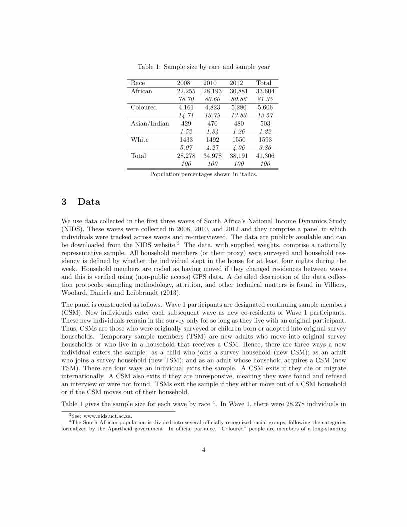
Table 1: Sample size by race and sample year

Race 2008 2010 2012 TotalAfrican 22,255 28,193 30,881 33,604

78.70 80.60 80.86 81.35Coloured 4,161 4,823 5,280 5,606

14.71 13.79 13.83 13.57Asian/Indian 429 470 480 503

1.52 1.34 1.26 1.22White 1433 1492 1550 1593

5.07 4.27 4.06 3.86Total 28,278 34,978 38,191 41,306

100 100 100 100

Population percentages shown in italics.

3 Data

We use data collected in the first three waves of South Africa’s National Income Dynamics Study(NIDS). These waves were collected in 2008, 2010, and 2012 and they comprise a panel in whichindividuals were tracked across waves and re-interviewed. The data are publicly available and canbe downloaded from the NIDS website.3 The data, with supplied weights, comprise a nationallyrepresentative sample. All household members (or their proxy) were surveyed and household res-idency is defined by whether the individual slept in the house for at least four nights during theweek. Household members are coded as having moved if they changed residences between wavesand this is verified using (non-public access) GPS data. A detailed description of the data collec-tion protocols, sampling methodology, attrition, and other technical matters is found in Villiers,Woolard, Daniels and Leibbrandt (2013).

The panel is constructed as follows. Wave 1 participants are designated continuing sample members(CSM). New individuals enter each subsequent wave as new co-residents of Wave 1 participants.These new individuals remain in the survey only for so long as they live with an original participant.Thus, CSMs are those who were originally surveyed or children born or adopted into original surveyhouseholds. Temporary sample members (TSM) are new adults who move into original surveyhouseholds or who live in a household that receives a CSM. Hence, there are three ways a newindividual enters the sample: as a child who joins a survey household (new CSM); as an adultwho joins a survey household (new TSM); and as an adult whose household acquires a CSM (newTSM). There are four ways an individual exits the sample. A CSM exits if they die or migrateinternationally. A CSM also exits if they are unresponsive, meaning they were found and refusedan interview or were not found. TSMs exit the sample if they either move out of a CSM householdor if the CSM moves out of their household.

Table 1 gives the sample size for each wave by race 4. In Wave 1, there were 28,278 individuals in

3See: www.nids.uct.ac.za.4The South African population is divided into several officially recognized racial groups, following the categories

formalized by the Apartheid government. In official parlance, “Coloured” people are members of a long-standing

4

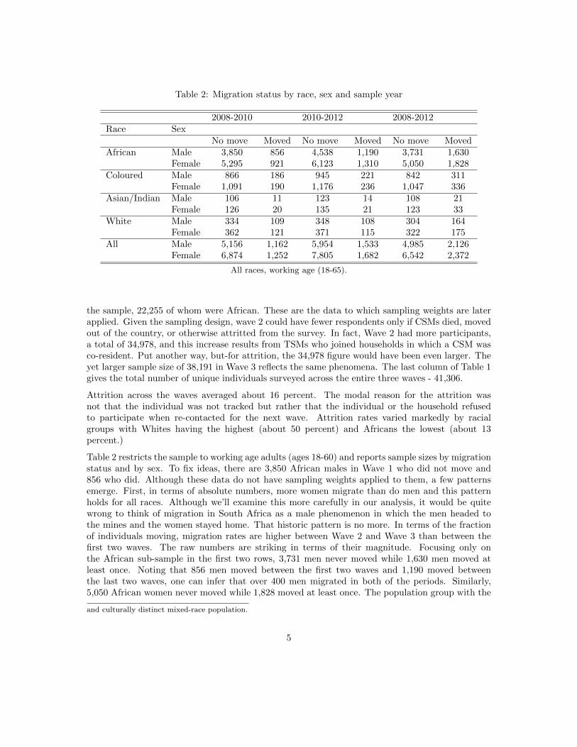
Table 2: Migration status by race, sex and sample year

2008-2010 2010-2012 2008-2012Race Sex

No move Moved No move Moved No move MovedAfrican Male 3,850 856 4,538 1,190 3,731 1,630

Female 5,295 921 6,123 1,310 5,050 1,828Coloured Male 866 186 945 221 842 311

Female 1,091 190 1,176 236 1,047 336Asian/Indian Male 106 11 123 14 108 21

Female 126 20 135 21 123 33White Male 334 109 348 108 304 164

Female 362 121 371 115 322 175All Male 5,156 1,162 5,954 1,533 4,985 2,126

Female 6,874 1,252 7,805 1,682 6,542 2,372

All races, working age (18-65).

the sample, 22,255 of whom were African. These are the data to which sampling weights are laterapplied. Given the sampling design, wave 2 could have fewer respondents only if CSMs died, movedout of the country, or otherwise attritted from the survey. In fact, Wave 2 had more participants,a total of 34,978, and this increase results from TSMs who joined households in which a CSM wasco-resident. Put another way, but-for attrition, the 34,978 figure would have been even larger. Theyet larger sample size of 38,191 in Wave 3 reflects the same phenomena. The last column of Table 1gives the total number of unique individuals surveyed across the entire three waves - 41,306.

Attrition across the waves averaged about 16 percent. The modal reason for the attrition wasnot that the individual was not tracked but rather that the individual or the household refusedto participate when re-contacted for the next wave. Attrition rates varied markedly by racialgroups with Whites having the highest (about 50 percent) and Africans the lowest (about 13percent.)

Table 2 restricts the sample to working age adults (ages 18-60) and reports sample sizes by migrationstatus and by sex. To fix ideas, there are 3,850 African males in Wave 1 who did not move and856 who did. Although these data do not have sampling weights applied to them, a few patternsemerge. First, in terms of absolute numbers, more women migrate than do men and this patternholds for all races. Although we’ll examine this more carefully in our analysis, it would be quitewrong to think of migration in South Africa as a male phenomenon in which the men headed tothe mines and the women stayed home. That historic pattern is no more. In terms of the fractionof individuals moving, migration rates are higher between Wave 2 and Wave 3 than between thefirst two waves. The raw numbers are striking in terms of their magnitude. Focusing only onthe African sub-sample in the first two rows, 3,731 men never moved while 1,630 men moved atleast once. Noting that 856 men moved between the first two waves and 1,190 moved betweenthe last two waves, one can infer that over 400 men migrated in both of the periods. Similarly,5,050 African women never moved while 1,828 moved at least once. The population group with the

and culturally distinct mixed-race population.

5

highest proportion of migrants is that of Whites, while the figure is lowest for Asian/Indians.

While all four population groups are included in NIDS, we focus our analysis on Africans. We donot include Whites for several reasons. The household dynamics underlying the migration decisionare massively different for this group. The multi-generation households that are such an integralpart of the demographic landscape of South Africa are not very present. Much of the observedmigration is due to “working age” adults going to or from university, and finally the data aresubject to high attrition rates. We also do not include the Asian/Indian population group. Inaddition to many of the issues that pertain to Whites, there is also a small-numbers problemsuch that drawing any inferences about nation-wide patterns for this group would be problematic.Finally, we also do not include the Coloured population group, although this is more of a closecall.5 The Coloured population is somewhat geographically concentrated and is less likely to livein multi-generational households or in “skip generation” households, in which grandparents cancare for grandchildren. Each of these attributes make the migration decision different than it isfor the African population. When observed, migration by Coloured respondents involves shorterdistances and fewer city changes, so it seems to be a different sort of choice than migration by Africanrespondents. Finally, the African population comprises about 83 percent of the (unweighted) sampleso we retain the vast majority of our data with our focus on Africans.

4 Descriptive Analyses

We begin with descriptive analyses of internal migration. These set the stage for the analysis ofthe causal impact of moving that follows. We focus our descriptive analysis around four questions.First, how many South Africans live in households impacted by migration? Second, when individualmigrate, do they move across communities or within and, when moving across communities howmuch migration is of the traditional rural to urban sort and how much is within urban, within ruralor even urban to rural? Third, what happens to the incomes of movers versus non-movers? Finally,what are the correlates of migration? That is, who moves as predicted by observables. This beginsto speak to the selection issue.

4.1 The prevalence of households impacted by moving

Table 2 provided a simple count of migrants. This count, though, vastly understates the numberof South Africans impacted by migration. Measuring the number of South Africans impacted bymigration is a multi-layered exercise. Because migration typically involves moves other than an enmasse move of the entire household, many household members other than the mover are impacted.Consider an unemployed 27 year old woman living in a 5 person household. If she moves and joinsa 2 person household, she leaves 4 members of the trailing household. Assuming someone in thattrailing household earned an income, the per capita income of the 4 trailing household membersrises with the migration ceteris paribus. And again assuming the migrant remains unemployed, shedrags down the household per capita income of the two members of the receiving household. Inthis example, there are 7 people impacted by the move. Table 3 counts the number of individualsin our sample who are and who are not impacted by a move, and when someone is affected by a

5We report key results including Coloured respondents in the Appendix.

6

move, we report how many are in trailing households and how many are in receiving households.We perform this exercise for moves between 2008 and 2010, for moves between 2010 and 2012, andfinally for any move during the span of the sample.

We begin with a discussion of the top panel of Table 3. From 2008 to 2010, 26.99 percent of Blacksin our sample were affected by a move into or out of their household. For the 2010-2012 period,the figure jumps to 39.54 percent, and over the four years spanning our data, over half of all Blackslived in a household that either sent or received a migrant. This strikes us as a stunningly highnumber for a period as short as four years. The fact that migration was more prevalent during therelative macroeconomic upswing than during 2008-2010 is suggestive of moving to opportunity asopposed to a push out of the nest, but we reserve this for more careful analyses below.

The percentages reported for trailing and receiving households are given in the second, fourth, andsixth columns for the last two rows of the top panel. Of households that were affected by a moverin the 2008-2010 period, 80 percent had someone migrate out of the household while 55 percenthad someone move into the household. This highlights an important and somewhat surprisingphenomenon. Many households that send a migrant also receive a migrant during the same period.(To fix ideas, both of the figures could theoretically be 100 percent if every household both sentand received a migrant.) The pattern of more people being affected by trailing a migrant than byreceiving one holds throughout the sample period.

Because of how the sample is constructed with the inclusion of Temporary Sample Members (TSMs),we were concerned that the figures in the top panel of Table 4 may not be representative. Toillustrate this concern, consider who joins the sample in Wave 3. These new sample members, bydesign, are either members of a household that was joined or formed by a migrant or the TSM ishim/herself a migrant into a household of CSMs. In order to better understand the extent of thispossible bias, we restricted our sample to the 2008 Wave 1 sample. Using only these individualsand following them through time, we repeat the analysis of the top panel and report results in thebottom panel of Table 3. We find that the large proportion of the sample impacted by migrationis in fact not an artifact of the sample design. If anything, the fraction of individuals affectedby migration is a bit larger. Using the entire sample over the four year span, 52.48 percent wereaffected and this figure rises to 54.15 percent when only Wave 1 sample members were included.The majority of Black South Africans lived in a household affected by migration.

4.2 Type of move

Table 4 speaks to the types of moves for working age (18-60) Blacks. The rows delineate themoves by urban versus rural while the columns note whether the move involved a change in therespondent’s District Council. District Councils are a more granular geographic unit than justProvince. There are 53 District Councils in South Africa and they vary widely in terms of size andpopulation. While they sometimes contain both urban and rural areas, they do not cross Provincialboundaries and rarely does an urban area lie in more than one District. For this descriptive analysis,we use the within and across District Council groupings to proxy for distance moved.

There are two key messages in Table 4. A half century of models of migration have focused onthe role played by rural to urban migration in economic development. Migration in South Africais more nuanced (as one would expect vis-a-vis a model) and, perhaps unexpectedly, just plain

7

different. In the 2008-2012 period, moves to rural areas were only slightly less common than movesto urban areas. This is a pattern that holds throughout the sample. While most moves were to ruraldestinations, most moves in the 2008-2012 period were from urban areas. The first key message,then, is the empirical prevalence of moves to rural destinations and from urban areas. Additionally,the vast majority of moves were within categories - most people moved within urban areas or withinrural areas. The third key point in Table 5 is that about 3 out of every 5 moves were within aDistrict Council. Most moves result in relocation not that distant from what had been home.

4.3 Income changes and migration

Table 5 reports changes in log per-capita household income by whether or not the respondent movedand by gender of the respondent. The sample includes all Blacks.6 Focusing first on the 2008 to2010 period, non-movers saw household per-capita incomes rise by about 4.3 percent. (All dataare in real terms.) This figure was about the same for males and females. Over the same timespan, male movers had an increase in per-capita household income of 25.6 percent and females 11.5percent. For the 2010-2012 period, a period during which the economy was picking up, non-movershad in increase in per-capita household income of about 18-19 percent. Female movers saw incomesrise by 51 percent while male movers experienced a 43 percent increase. Over the entire sampleperiod, non-movers saw an increase in per-capita household income of about 21.7 percent while thefigure for movers was about 43 (female) to 44 (male) percent. These strike us as large differencesin income over a relatively short time span.

4.4 Who moves?

We conclude our descriptive analyses with an examination of just who moves. This is a precursorto our analysis of the causal impact of moving. As seen in Table 5, income growth was higherfor movers. Of course, to the extent that movers might be better educated, more ambitious, andwith better employment-related skills, these movers might have earned higher incomes even if theyhad not moved. Table 6 provides a first pass at analyzing just who moves. That table gives theresults of a linear probability model regressing whether or not the respondent moved on respondentattributes in the wave prior to the move. The sample consists of working age Blacks. The firstcolumn gives results for moves between waves 1 and 2, the second for moves between waves 2 and3 and the third for the entire period. Columns 4 and 5 break out the sample by sex.

Two key messages emerge from this simple descriptive analysis. First, as a general matter, moverstend to be younger and better educated. This is not surprising and it’s true throughout the sample.Second, there are differences across the waves in terms of who moves and this provides someinitial evidence that migrants during the downswing may differ from those during the recovery.For example, in the macroeconomic downswing, movers tended to have partners while during theupswing they tended to be single. (Overall, the two statistically precise effects cancel one anotherout.) In the downswing, movers came from smaller households while in the upswing they came fromlarger households. Finally, in the upswing, movers were less likely to come from a female-headedhousehold but were more likely to be female. To the extent that selection on observables matters,it matters differently across the business cycle.

6Figures in this table reflect sample weights.

8

5 Framework

5.1 Framing the Question

In South Africa, as in many African countries, pooling of income within the household is the norm.As a result, we focus on household income and, to account for varying household sizes, we arriveat our outcome variable, household per capita income. When computing this measure, remittancesdeserve careful attention since they can potentially appear twice in the data. If both the sending andreceiving households are surveyed, remittance income accrues first to the sender (through earnings)and then to the receiver (through remittances.) Because many remittance networks arise as a resultof migration, the returns to migration may be distorted if remittances are not handled with care.We assign remittances to the recipient household, not the trailing household.

In the presence of income pooling within the household, the economic impact of migration is nu-anced. In order to be clear just who comprises the household at a given point in time, it is helpfulto establish some notation.

Consider a given household. Denote the set of individuals who migrate between period t and t + 1by M . The trailing household members are denoted T . This is the set of individuals who co-residewith M in period t but not in t + 1. The members of the receiving household are denoted R. Thisis the set of individuals who co-reside with M in period t+1 but not in period t. Table 7 illustratessome examples of household composition with migration and helps fix ideas.

Return now to the question posed at the outset, “Is migration a way of getting ahead?”

The first line in Table 7, Example 1, gives the example of a household that moves en masse. That is,the members of the household in period t are the same as the members in t+ 1. Because householdcomposition does not change, it’s straightforward to determine if the household members are betteroff with the move. Individual incomes within households are observed in NIDS in period t andt + 1, so one simply computes per capita household income before and after the move to measurewhether migration left the household with a higher or lower per capita household income. Thissituation is rarely observed in the data – with the exception of one person households that migrate,the migrating household typically loses or gains members.

Example 2 looks at migration from the perspective of the migrants when only some members ofthe period t household migrate. In this example, the only household members in common acrossthe two periods are the migrants (or migrant, since it may be an individual rather than a group ofmigrants). If the question being asked is “Is migration a way of getting ahead for the migrants?,”example 2 is the appropriate comparison. Note that in the presence of income pooling, it’s entirelypossible for the migrant’s individual income to fall with migration but for her per capita householdincome to rise (and vice versa.) Because Mt+Tt, the migrants’ original household, and Mt+1+Rt+1,the migrants’ new household, are each observed in NIDS, it is straightforward to measure whetheron average migrants’ per capita household income increases or decreases with migration.

Next consider Example 3 in Table 7. A comparison of the per capita household incomes of Mt +Tt

to that of Tt+1 is answering yet a different and still well-defined question. Example 3 asks “Whathappens to the trailing household in the presence of migration?” Still using per capita householdincome as the appropriate measure of income, this framing analyzes whether migration is good forthose household members who live in the household that the migrants left. If for example, it’s the

9

slackers who leave the nest, we measure how this migration has benefited the trailing householdmembers. Or if it’s the most productive members who leave, how badly are trailing householdmembers harmed by migration? In our data, Mt + Tt and Tt+1 are each observed. Hence it’sstraightforward to measure whether on average trailing household members experienced higher orlower per capita household incomes from migration.

Finally, consider Example 4 in Table 7. This comparison asks whether migration benefits thereceiving household. This too is a well-defined variant of the core question “Is migration a way ofgetting ahead?” This time, though, the question is viewed from the perspective of the receivinghousehold. As a general matter, Rt would not be observed in NIDS. This is the income of thehousehold that receives the migrants (at which point those household members become TemporarySample Members) in the period before the migrant arrives. It turns out, though, that in manycases, Rt is in fact observed in NIDS. This is because there are so many households that both sendand receive migrants. For example, when the household that receives a migrant in 2010 also sent amigrant in 2008, we observe both Rt and Rt+1. Hence, we are able to measure whether on averagereceiving a migrant is a way for a household to get ahead.

Each row in Table 7, then, frames the question “Is migration a way of getting ahead?” from adifferent perspective. The first row asks the question from the perspective of the household thatmoves en masse. The second asks from the perspective of migrants who left one household to joinanother. The third asks the question from the perspective of the household members left behindwhile the last asks from the perspective of the household that received the migrants. We answereach.

5.2 Econometric Strategies

We return to the core question of whether migration is a way of getting ahead. To measure thecausal impact of migration, we need a way to infer how a migrant (or a migration-affected household)would have fared had they not migrated. This, of course, is not observed so any measurement of thereturns to migration must be obtained from comparing migrants to non-migrants. This immediatelyraises the problems of identifying comparable non-migrants, and controlling for the role of selection.Selection appears in two forms for migration - selection into migration, and selection of destination.We do not make any attempt to address the latter, so our estimates of the returns to migrationinclude destination effects.

Given that selection is inherent in the migration decision, the cleanest way of addressing it is torun a RCT. This is the approach favored by McKenzie et al. (2010) and Brian et al. (2011). ThoseRCTs involved migration from Tonga to New Zealand for applicants to a lottery who had proofof employment in New Zealand, and financially incentivizing temporary migration in Bangladesh,respectively. Our goal is more expansive. We wish to understand whether migration is a way ofgetting ahead for the millions of Black South Africans who elect to move. While one can imaginean RCT that spoke to this question, the practicalities of actually implementing such an RCT acrossa country as ethnically and geographically diverse as South Africa are daunting. Rather, we relyon non-experimental data. Given this, the next question is the choice of estimator.

An often preferred approach to the endogeneity induced by selection bias is an instrumental variables(IV) estimator. The advantage of the IV estimator is that it addresses selection based both on

10

observable and unobservable characteristics. The feasibility of this approach hinges on whetherthere are good instruments. In our context, instruments need to be correlated with the migrationdecision and orthogonal to income shocks. This is a tall order to fill. While there are special caseswhen a clever instrument exists, we have come up short.7 This is in part due to the scope of thequestion we address - migration on a national level.

Truly randomly migration status is very seldom observed outside an experimental setting (andhistory has not looked kindly on those examples that do exist.) Instead of looking for an estimationstrategy that recovers the impact of migration were migration status randomly assigned acrossthe entire population, we instead derive the effect of migration for those who moved (the averagetreatment effect on the treated, in the language of program evaluation), and we do so using matchingestimators. This approach simply does not speak to the economic impact of a policy that reducedthe costs of migration for the entire population. But for the question posed at the outset, “Ismigration a way of getting ahead?”, our matching estimators are on point.

Matching estimators in the context of migration were discussed by McKenzie et al. (2010). Ham, Liand Reagan (2011) used matching very successfully to estimate the returns to migration for youngmen in the US. Matching estimators are generally considered inferior to experimental estimatorsbecause they can control for selection only on observables. In formal terms, matching assumes thatthe distribution of potential incomes of migrants and non-migrants are independent of migrationconditional on the set of covariates, X. Let D denote migration status, with D = 1 for migrants(migrant-households) and D = 0 for non-migrants. Similarly, Y1 is income after migration and Y0

is income for non-migrants in the corresponding period. Then the assumption underlying matchingis that

(Y1, Y0) ⊥⊥ D|X (1)

If this is true, then conditional on covariates X, non-migrants have the same income distributionthat migrants would have experienced without migration, and migrants have the same incomedistribution that non-migrants would have experienced had they migrated. Matching estimatorscan then calculate the return to migration by creating a weighted sample of non-migrants such thatthe distribution of observable characteristics in each group is the same. However, assuming thatthe returns to migration do not affect the migration decision, even with a large selection of controlvariables, is probably wrong.

Heckman., Ichimura, Smith and Todd (1998b) and Rosenbaum and Ruben (1983) demonstrate thata weaker condition is sufficient for a valid matching estimator, namely

E (Y0|P (X), D = 1) = E (Y0|P (X), D = 0) (2)

where P (X) = Pr (D = 1|X). The use of the index P (X) avoids the dimensionality problem thatarises with using a large number of covariates, and only mean-independence of the non-migrationincome is assumed. This amounts to allowing the returns to migration to differ across migrantsand non-migrants, while requiring that the non-migration incomes of each group have the samemean. Individuals can self-select based on their expected post-migration income, provided their

7McKenzie et. al. use distance to the Department of Labor office since it turned out that simply knowing abouthow the lottery worked was an important determinant to whether one applied for the lottery. In an entirely differentcontext, Munshi (2003) used rainfall in Mexican villages as an instrument for the social networks that ended upbeing important for migration decisions.

11

incomes without migration do not differ. This is the result that Ham et al. (2011) use to justifytheir matching estimator. Because it does not claim mean equality for Y1, this estimator cannotbe used to measure the average return to migration for the population, or even for a sub-sample oflikely migrants. It can only measure the returns for those who migrated, because only Y0 is assumedequivalent for migrants and non-migrants. It does not speak to the income that non-migrants wouldexperience if they migrated, but only to the income that migrants would experience had they notmigrated.

Even in this less restrictive case, matching estimators may still be biased compared to experimentalestimators. The extent and sources of this bias was studied in detail by Heckman, Ichimura andTodd (1997) in their evaluation of non-experimental relative to experimental methods using a USjob-training program. They identify three contributors: nonoverlapping support between treatmentand control populations; different distributions of covariates X within the two populations; andgenuine selection bias due to selection on unobservables. In the cases they examine, the largershare of measured bias was due to the first two contributors, not to true selection bias. If matchingmethods are correctly applied, these first two sources of bias can be eliminated and the remainingbias in measurements, due to selection on non-observables, will be small.

The two additional sources of bias that commonly arise in nonexperimental evaluations are dueto geographic mismatch between treatment and control groups, and the use of different surveyinstruments (Heckman et al. (1997)). For our purposes, the latter is not of concern. Informationon both migrants and non-migrants was collected in the same nationally representative survey.We additionally have access to sufficiently detailed geographic information to place migrants andnon-migrants into the same (pre-migration) labor markets, which increases the plausibility thatY0 is truly equivalent for both groups. The limiting factor in practice is sample size, which pre-vents matching within District Council. We instead match within the same type of labor market,explained further in Section 5.2.1.

Many migration papers (and many papers studying income effects more broadly) advocate for theuse of differenced data. We use differenced idata, but this does not generate the same benefits as itusually does. In general, differencing is an effective strategy for dealing with unobservable individualattributes that do not change over time and for which the impact on income is time invariant. In thiscontext, DD estimators, when applied to panel data, address selection on unobservables. The firstdifferences approach, though, runs into problems when migration involves a change in householdcomposition and when income is measured by household per-capita income (as in Examples 2, 3,and 4 in Table 7.)

An example illustrates the issue. When the household is comprised of multiple individuals, correlatesof household per capita income for individual i include information about other members of i’shousehold. Some of these correlates will be unobserved. For example, if individual i’s householdincludes a cousin, William, who is lazy and stupid, this would exert a negative influence on theresidual in a regression of i’s per capita household income on a set of observables. If William isin the household both periods, differencing the data will sweep out this unobservable influence onhousehold per capita income. For Example 1 in Table 7, DD estimators work as expected. Whenmigration involves a change in the household composition, though (as in Examples 2, 3, and 4 inTable 7), DD estimators run into problems. This is because the unobservable that captures cousinWilliam’s negative impact on household per capita income in period t may no longer be presentin period t + 1. Hence, when household composition changes, in the presence of income pooling

12

first differencing the data no longer sweeps out all the time invariant unobservables that mightimpact household per capita income, and which might be correlated with migration. Because ofthis issue, we rely on matching estimators although we report some results in the appendices witha DD estimator for the sake of comparison.

Independent of exactly which matching estimator is used and on which variables we base the match,a logically prior question is just which match identifies the causal impact of migration in each ofthe four examples in Table 7. That is, on what should one match to identify the causal impact ofmigration on the individual migrant (Example 1), the migrant who switches households (Example2), the trailing household (Example 3), and the receiving household (Example 4)?

In each case, we start by noting the change in income that is observed in the data. We thenask, “What is the unobserved counterfactual change that, when compared to the actual change,identifies the causal impact of migration?” Answering this requires pinpointing just what part ofthe counterfactual change is unobserved and then selecting the appropriate match to “proxy” forthis unobserved.

In Example 1, we observe the change in per capita household income for the migrant whose house-hold moved en masse. We want to know how that migrant’s household per capita income wouldhave changed had they not moved. Since we observe the migrant’s income in period t prior to themove, the missing piece of information is the migrant’s per capita household income in period t+ 1had she not moved. The match, then, looks for someone who is like the migrant in period t but whodid not move. This non-mover’s income in period t+1 is our estimate of what the migrant’s incomewould have been and so allows us to estimate the counterfactual income change against which tocompare the actual income change. The difference is the causal impact of migration.

Example 2 is similar. We observe the actual change in per capita household income for the migrantwho, in this case, changes households. We want to know what the migrant’s per capita householdincome would have been if she had stayed in her original household. The match, then, looks foran individual like the migrant, in a household that is like the migrant’s in period t but did notexperience a migration event and asks what their period t+ 1 per capita household income is. Thedifference between the migrant’s actual change in per capita household income and the matchedestimated of what it would have been absent leaving their original household is the causal impact ofmigration. It might seem that a good proxy for the migrant’s per capita household income in t+ 1but for the move is the observed per capita income of the trailing household members (those whodid not move.) This would be appropriate if the household were atomistic and did not somehowre-optimize after the departure of the migrant. This is probably not defensible.

In Example 3, we observe the actual change in per capita household income for the trailing house-hold. The unobserved counterfactual is what this change would have been had the migrant notdeparted. We observe the trailing household’s actual per capita income in period t so the unob-served is the trailing household’s period t + 1 per capita household income but for the departureof the migrant. This is identical to the unobserved in Example 2. The only difference is thatin Example 3, we compare the counterfactual change in income to the trailing household’s actualchange while in Example 2 we compare the counterfactual change to the migrant’s actual change.Our matching algorithm, then, again looks for a household that is like the migrant’s in period t butdid not lose a household member (or members) due to migration and then asks what their periodt + 1 per capita household income is.

13

Example 4 highlights the causal impact of migration on the receiving household. We observe theactual change in per capita household income for the receiving household. The counterfactual ishow the receiving household’s per capita household income would have changed if it had not takenin the migrant(s). We observe the receiving household’s period t income so the unobserved is thereceiving household’s income in t+ 1 had they not taken in the migrant(s). The match, then, findsa household that is like the receiving household in period t but which did not receive a migrant andasks what that household’s period t + 1 income is.

Our choice of matching estimators fall into two categories: propensity score matching, guided pri-marily by the conclusions from Ham et al. (2011); and Mahalanobis matching on multiple covariates,as developed by Abadie and Imbens (2006). Similarly to Ham et al. (2011) and McKenzie et al.(2010), we use several different specifications to get a range of estimates and demonstrate the overallrobustness of our results. Two remaining implementation issues are which observables are used toconduct the match and which particular estimators are used. Each is discussed in turn.

5.2.1 Conditioning variables

The same set of conditioning variables is used for all our specifications. Ham et al. (2011) demon-strates, specifically in the context of measuring the return to migration using matching estimators,that a comprehensive approach is best. All variables that affect the income or wage should beincluded, as well as all available variables that are correlated with the underlying variable drivingthe migration decision. Thus, traditional income determinants such as age and education will beincluded as well as variables that potentially influence the migration decision - household structure,location and prior earnings. We do not condition on full labor market histories to avoid excludingindividuals with limited participation or wage information and individuals who are migrating fornon-labor market reasons. The exact variables used are quartics in age and education, as wellas an interaction between age and education, gender, marital status8, province, community type,interactions between all the above and gender, and income in the survey wave prior to migration.Household-level variables included are the mean age and education of the household, householdsize, whether it is rural or urban, whether it contains a pensioner, a female pensioner, a child underseven or a child under three, and the fraction of the household that is female, employed, prime-aged(18-65), and the fraction that are under eighteen, under sixteen9, under seven10 or under three. Wematch within the type of community in which the household resides so as to capture the potentialimportance of local or regional labor markets11, so that migrants must be matched to non-migrantswho reside in the same type of labor market as they did initially.

8Due to the ubiquity of long-standing cohabitation of non-married couples in South Africa, individuals who cohabitwith a partner are counted as ‘married’.

9These children cannot legally work and their guardians are eligible for Child Support Grants.10Children under seven do not have to be enrolled in school.11The four potential types are urban formal, urban informal, rural formal, and former Tribal Authority. The latter

two differentiate between rural areas with reasonably well-functioning local labor markets and infrastructure, andrural areas in the formerly Black areas of South Africa, which have a long history of low government provision ofservices and infrastructure, very low formal employment and very high poverty rates

14

5.2.2 Matching Estimators

Propensity score matching has been the traditional solution to the dimensionality problem createdby having many covariates on which to match. A probit (or logit) model is used to calculate theprobability that any one individual moves given their covariate values. Movers are then matched tonon-movers with similar probabilities of moving. What does similar mean? The simplest approachis to use nearest neighbor matching - the mover is matched to the non-mover with the closestpropensity score value. However, this is inefficient - it uses only one of many potential matchesand thus discards much useful information. A partial solution is to use an average of the K nearestneighbors (K=2,3,etc) instead of the single nearest neighbor. This reduces the standard errors ofthe estimates, as more information is available, but is problematic because the ‘nearest’ neighborsfor a particular individual will be of varying closeness depending on the density of the data aroundthat individual.

Heckman et al. (1997), Heckman, Ichimura and Todd (1998a) and Heckman. et al. (1998b) incor-porate local regression into matching. Instead of choosing one (or K) control individuals to matchto each treated individual, everyone with a propensity score within a window around each treatedindividual’s propensity score is used to create a weighted average counterfactual income for themigrant, with weights decreasing in their distance from the migrant. This has the advantage ofincreasing the information used (and thus decreasing the variance of the estimates) while limitingthe increase in bias through the weighting procedure. Fan and Gijbels (1996) recommend the useof a local linear, or at times a local cubic, regression.

Frolich (2004) argues that kernel regression (essentially a local regression of degree zero) is morerobust to specification errors than linear regression. However, this problem can be partially ad-dressed through the use of a variable bandwidth and is most problematic when the control group isnot substantially larger than the treatment group (less than five to one). The ratio of non-migrantsto migrants among Africans is closer to four to one, and the ratio of those affected by migration tothose unaffected is almost one to one, so this is a concern for our analysis. However, local linear re-gression matching is more robust to asymmetric distributions of control individuals around treatedindividuals, which is a feature present in our data (Caliendo and Kopeinig 2008).

Practical techniques and asymptotic properties for matching on multiple variables were most re-cently put forward by Abadie and Imbens (2006). Instead of creating an index measure of similarityas the propensity score methods do, this approach attempts to match treated and non-treated in-dividuals on the values of significant determinants directly. Matches are generated by minimizingthe Mahalanobis distance between observations.

We employ multiple estimators to determine the robustness of our estimates. Our preferred esti-mator uses a local linear regression with a normal kernel, to make use of more information than anearest neighbor match while limiting the bias from decreased match sensitivity.

6 The Causal Impacts of Moving

We organize our base case results by first examining the causal impact of migration from themigrant’s perspective. We then conduct our analyses from the perspective of the trailing household

15

and finally from that of the receiving household.

6.1 Returns to Migration for the Migrant

Table 8 presents the returns to migration for the migrant. We analyze returns for moves thatoccurred between 2008 and 2010, moves during 2010-2012, and again for any move between 2008and 2012. Within each of these time periods, the first two columns give the estimates using (log)household per-capita income and the third uses (log) individual income, for comparison to othermigration papers. In the first two columns, the first uses a Mahalanobis matching estimator andthe second a propensity score matching estimator.

We begin with the first row of Table 8. Because the dependent variable is log income, coefficientsare interpreted as the percentage change in income. To fix ideas, the causal impact of migrationacross all Black South Africans was an increase in household per capita income of 24.88 percent inthe 2008-2010 period when using the Mahalanobis matching (M. kernel, hereafter) estimator and28.4 percent when using the propensity score (P. kernel, hereafter) estimator. From 2010 to 2012,these already substantial returns increased to 33.0 and 38.9 percent respectively. Across the entiresample, the causal impact of migration was a 30 percent increase in household per capita income(for both estimators.) All of these returns are quite precisely estimated.12

For each of these time periods, we also include an estimate of the return to migration if we use logindividual income instead of log household per capita income. These results are presented simplyfor purposes of comparison. These would be the appropriate estimates if households did not poolincome. This is the assumption adopted in much of the migration literature and by comparingthis (P. kernel) estimate with the P. kernel estimate using household per capita income, one cansee just how different the results are. For 2008-2010, there is no return to migration when lookingat individual income and in 2010-2012 and 2008-2012, returns using individual income are abouthalf what they are when using household per capita income. These comparisons, though, are farfrom exact, since the samples with the two income measures differ. Although no households havezero household income, many individuals do and these individuals are excluded from an analysis oflog individual income. In any case, the assumption of no income pooling is untenable in a SouthAfrican context. Henceforth, we focus on the results using household per capita incomes.

There are at least three high-level messages. First, these returns to migration are large. A 25-28% increase in 2008-2010 and a 33-39% increase from 2010-2012 are big changes. It’s importantto recall that migration is not a rare event. Second, the M. kernel and P. kernel estimators givesimilar estimates, so the large returns are not an artifact of using a particular estimator. For 11 of

12Unlike some of the recent literature on matching, we do not bootstrap the standard errors. Imbens (2014) andAbadie and Imbens (2008) demonstrate that bootstrapping is not in general a valid way to calculate standard errorsas matching estimators are not asympototically linear. Instead, we use the standard error procedure proposed inAbadie and Imbens (2006) and available in the Stata program psmatch2, written by Leuven and Sianesi (2003). Theoverall idea of this procedure is that, to estimate consistent asymptotic variances for the sample average treatmentfor the treated (as opposed to for the population ATT), one does not need consistent estimates of the conditionaloutcome variances for treated and control groups at all values of the covariates. It is sufficient to have the averageof these variances over the distribution of outcomes, which, when weighted with the inverse probability of groupassignment (treatment and control, respectively), can be used to construct a consistent estimator of the variance ofsample ATT. Alternative standard error treatments are reported in Section 7.

16

the 15 pairs of M kernel and P. kernel estimates, the two are quite similar. Third, the returns tomigration are much higher during the macroeconomic upswing than during the downswing.

The returns to migration are heterogeneous and the next four sets of rows of the table illustratethis for particular cuts of the data. For males with a Matric13 during the 2008-2010 period, returnsare not sufficiently precisely estimated to allow a comparison to males without the Matric. Pointestimates, though, suggest lower returns for males with the Matric than without. During the moreexpansionary 2010-2012 period, returns were much higher for males who had the Matric. Indeedthe return to migration for males with a Matric were a stunning 55-57% during 2010-2012 (andthese are quite precisely estimated.) Across the entire sample period, the return to migration was10 to 15 percentage points higher for males with a Matric than for males without it.

For females, returns to migration tend to be slightly less than those for males. As was the casefor males, returns are higher for females with a matric than without and the gap is most evidentduring the upswing of 2010-2012.

The broad pattern is one in which migration is a way of getting ahead for the migrant and that thereturns are substantially higher during the macroeconomic upswing. Even during the downswing,though, migration enhances migrants’ incomes. The results support a “moving to opportunity’ viewof migration rather than a “push out of the nest” view.

6.2 Returns to Migration for the Trailing Households

We turn next to the impact of migration on the trailing household. The first row of Table 9 compareshouseholds who ever sent a migrant to those that did not. Trailing households benefit from themigrant(s) leaving the household. These returns are fairly steady across estimates and time periods.Over the 2008-2012 span, trailing households saw per capital household incomes increase 17-22%relative to like-positioned households that did not send off a migrant.

The next two rows of Table 9 separate out those households that had household member(s) leave inthe 2008-2010 period (“early”) from those who had member(s) leave between 2010 and 2012 (“late”).Trailing household per capita income rose about 20% when a household member(s) left early. Therewas no effect on 2010-1012 incomes from the 2008-2010 migration event– a result suggesting trailinghousehold member incomes respond quickly rather than with a lag to a migration event. Trailinghouseholds also saw incomes rise comparably when a household member(s) migrated in the 2010-2012 period. Household per capita income of the trailing household rose 22-25%. Prior to themigration event, household per capita income of what would become the trailing household waseither unchanged (M. kernel) or 5% higher (P. kernel). The latter effect is (barely) statisticallysignificant but it may be interpreted as violating the identifying assumption underlying causality.It may also be viewed as a (very modest) leading indicator to a forthcoming migration event.

The remaining rows divide households by whether they are urban or rural and by whether thehousehold head is male or female. The most notable result is the large increase in householdper capita income of a female-headed trailing household during the economic downswing. This isconsistent with the out migration of a household member who had been a drain on the household’spooled resources, and is consistent with the South African literature on household formation.

13To graduate high school South African students must pass “matriculation” exams. Thus, high school graduatesare said to “have a Matric” and we use the term as a short-hand for ”high school graduate”.

17

6.3 Returns to Migration for the Receiving Households

The returns to migration for the receiving household vary with the two estimators. Focussingfirst on the top row in Table 10, receiving a migrant either has no statistically significant impacton household per capita income (M. kernel) or a modest increase (P. kernel.) When we examinethe impact separately for households that received a migrant during the downswing versus duringthe upswing, the results are more striking. During the downswing, receiving a migrant increasedhousehold per capita income and the point estimates are large (17% for M. kernel and 30% forP. kernel although the former is imprecisely estimated.) Returns to receiving a migrant in theupswing are about half those in the downswing. Taken across the entire sample period, receivinga migrant has a modest positive impact on household per capita income, and for the M. kernelestimates, we can seldom reject that the impact is zero (note can we often reject that the M.kernel estimate is different from the larger P. kernel estimate.) The results support the notion ofselection of destination by the migrants. That is, migrants are not choosing to move to householdsin which their arrival will significantly decrease household per capita income. This might ariseeither because the migrant is altruistic or because the receiving household does not welcome anadditional household member when that migration event would result in decreased household percapita income.

6.4 Summing Up

Taken together, the broad picture is one in which migration significantly increases the householdper capita income of the migrant, assisted the trailing household members during the downswing,and had either no or a modest positive impact on receiving households. The results highlight thatmigration is not a zero sum event even in the presence of income pooling. During the downswing, themigrant, the trailing household and the receiving household all benefitted. This is consistent withmultiple scenarios, one of which is underemployed individuals who had been a drain on householdresources moving to opportunity (and finding it), hence benefitting all parties. During the upswing,again all parties tended to benefit from the migration event, but the largest gains were to the migrantherself. [More?]

7 Robustness of Results

We next examine the robustness of our results. A common concern with matching estimators is theirsensitivity to mis-specification and choices of conditioning variables. To address this concern, wecalculate the returns to migration using several different matching algorithms and estimate standarderrors for our preferred specifications using three methods common in the literature. These resultsare discussed in Section 7.1. We also test the sensitivity of our results to different definitions ofmigration. Finally, the concept of migration that we examine is very broad and may incorporatedifferent motives for and manifestations of movement between households and locations. To geta better sense of how these might differ by type of migrant, in Section 7.3 we examine returns tomigration by age of migrant and direction of migration. 14

14Unless otherwise noted, all results in this section use propensity score matching on a local linear regressionfunction and do not require exact matches on location type. Due to the smaller samples used here, it is not possible

18

7.1 Alternative matching algorithms and standard error calculations

A common concern with matching estimators is their sensitivity to mis-specification and choice ofconditioning variables. To address this concern, we compute the effects of migration using twelvedifferent estimators for each of the four questions discussed above - individual and household percapita income for the migrant, and household per capita income for the trailing and receivinghouseholds.15 For each case, we use four nearest neighbor matching estimators (with the numberof matches set to one, two, five and ten, respectively), a local linear regression matching estimatorand a kernel matching estimator, using both propensity score matching and matching on multiplecovariates (Mahalanobis matching). The set of matching variables ranges from the full set ofpolynomials and interactions used in the results reported in Section 6 to a parsimonious set ofdemographic and location controls. The results in all cases are similar, typically lying within one tofive percentage points of the preferred estimate. The more variable estimates are for the individualincome measure and for the receiving households. As noted in the text above, many individuals donot have personal income in one or other year, so the individual income measures may suffer fromboth selection bias (into the labor market), from small sample concerns, and from high variabilitywithin individual. The variability for receiving households seems to be primarily due to smallersamples.

Another point of concern for matching estimators is the calculation of standard errors. Thereare limited results on the asymptotic properties of matching estimators, though recent work byAbadie and Imbens16 suggests that the most common approach in the literature - bootstrappedstandard errors - does not yield correct standard errors and is in fact systematically biased. Theyinstead propose standard error corrections that provide consistent estimates of variances of sampleestimators by focusing on distribution-average variance. This is the approach used for our mainresults. However, our results are robust to alternative standard error treatments. Table 11 givesresults for individual migrants with household per-capita income, by gender and education leveland for each of the three migration periods. In the first, third and fifth column, standard errorsare bootstrapped. In the second, fourth and sixth column, standard errors are calculated usinganother correction commonly found in the literature, proposed by Lechner (2001). This estimatorexplicitly accounts for the fact that individuals in the control group are used as matches repeatedly,and performs equivalently well to bootstrap in simulated results ((Lechner 2002)). This methodcan only be used with K nearest neighbor matching, because kernel or regression matching usesmost control observations to calculate each counterfactual match. Thus, the coefficients in thesecolumns differ slightly from the others due to the use of nearest neighbor (K=10) matching insteadof local linear regression matching. The choice of standard error calculation does not affect thesignificance of our results. All coefficients remain significant, except those for high school graduatesbetween 2008 and 2010, which were insignificant in our main results as well.

Overall, we are confident that our results are not sensitive to our choice of matching algorithmor standard error treatment. While the coefficients vary slightly in response to different matchingalgorithms, the relative sizes and significance are not affected, and the variation is small for almost

to match within locations, so location type and province are treated as normal covariates in the calculation of thepropensity score.

15These results are available on request from the authors.16Abadie and Imbens (2002), Abadie and Imbens (n.d.), Abadie and Imbens (2006), Abadie and Imbens (2008),

Abadie and Imbens (2009)

19

all measures.

7.2 Alternative definitions of migration

Our main results use a broad definition of migration as any switch between households. Thismay include many local, short-distance moves that almost certainly do not involve changing labormarkets. We believe that this is a sound decision in a context of extended household networks andintra-household income sharing, because household composition is an endogenous response to theeconomic environment and family shocks. However, the more traditional definition of migrationinvolves long distance moves in which migrants change labor markets and travel significant distancesaway from their families. As another robustness check, we examine how our results change whenalternative definitions of migration are used. In Table 12, we present the returns to migration forthe migrant, in household per-capita income, by gender and education level, for three additionalmigration definitions. In columns one, four and seven, only individuals who have moved more thanthe median distance of a move are counted as migrants. This still amounts to a relatively low numberof kilometers moved - most of these migrants will have relocated within the same province. In thesecond, fifth and eighth columns, only individuals who have moved at least 50km are defined to bemigrants. In the third, sixth and ninth columns, only individuals who have changed districts areconsidered migrants. In US terms, this is somewhat equivalent to defining migration as switchingMSAs or counties. These three definitions are all stricter in the sense that many individuals whohave changed households, and are thus considered migrants in our main results, do not qualify asmigrants under them.

In almost every instance (the exception is female high school graduates between 2010 and 2012),the returns to migration under these stricter definitions are greater than those estimated under thehousehold change definition. We are thus confident that our main results are a lower bound on thereturns to migration.

An important qualification to the robustness of the results for individual migrants is that the resultsfor the associated households are less stable. In Table 13, we examine the returns to migration forthe associated households. In our main tables, 10 and 9, we classified households by whetherthey had sent a migrant or received a migrant, against a control group of households who haddone neither. However, many households did both. In Table 13, households are split into fiveoverlapping categories. Trailing and receiving households are defined as above. The second rowcompares households that only sent - and did not receive - a migrant to households that did neither.The fourth row compares households that only received a migrant to households that neither sentnor received one, and the fifth row compares households that both received and sent migrants tothose that did neither. The first thing to note is that very few households only received migrants.In fact, so few did so in the first period that we cannot estimate returns for them, and in thelater and overall periods, the numbers are still low. Secondly, in the later period, only-receivinghouseholds fared significantly worse than the comparison group. While trailing-only households didbetter than non-migrant households, they did not do as well as trailing households that includesenders and receivers. Finally, the largest gains from migration were experienced by householdsthat both sent and received migrants, ranging from 26% to 37%, which is on a par with the resultsfor individual migrants.

One potential interpretation of these results is that households that are more connected to the

20

networks created by migration do better than unconnected households. Additional results (notreported for brevity) indicate that households with more exposure to migrants, received or sent,experience higher income gains than households with less exposure. The few households thatonly received migrants are significantly less connected to the network, measured in this way, thanhouseholds that sent migrants or households that did both. We can argue that they are somehowatypical of the general migration experience. This is a very preliminary interpretation of resultsthat are based on very small sample sizes.

The main conclusion that we can confidently draw from Table 13 is that the results in Table 10are not representative of all receiving households, unless we believe that the majority of householdsthat receive migrants do actually send them as well.

7.3 Exploring returns to migration within sub-samples

Another relevant critique of any effort to measure the returns to migration is the likelihood that theeffects vary by group. As we saw above, our estimates differed by education category and gender.We present estimates for two other segmentations of society that plausibly have different migrationpatterns or motives: direction of migration; and age of migrant.

In development economics, migration is typically thought to take place from rural to urban areas.Table 4 showed that this is not the most common form of migration in South Africa, as themajority of the moves we observe are within urban or rural areas. Rural to urban moves aredisproportionately likely to be long-distance moves, however.17 It’s natural to think that migrationwithin urban areas may be a very different phenomenon than migration from rural to urban areas,so we next examine the effects of migration by the direction of migration. Four categories exist:urban to urban; urban to rural; rural to rural; and rural to urban. The migration effect for each ofthese types of move for each time period are displayed in Table 14.

There are substantial and significant differences in the income effects of migration depending onthe direction. As with all other calculations, the effects differ greatly depending on the timeperiod examined. There are two particularly noteworthy points shown in Table 14. First, movingfrom a rural to an urban area has income effects that dwarf those from any other type of move,ranging from 61% to 80%. This suggests that we are not wrong to think of this type of move asbeing an economic game-changer for migrants. Second, these effects are all precisely estimated andsignificantly different from each other, other than urban to rural migration, which is imprecise andindistinguishable from zero. This type of migration is less frequently observed than the others andis also more likely to be associated with income losses. This is evidence that some part of urban torural migration may consist of ‘failed’ migrants returning to poorer households, or perhaps adultsreturning home to retire. Overall, however, this cut of the data supports our result that migrationis associated with large and significant increases in income.

The same story is borne out when the results are split by age of migrant (shown in Table 15).The returns to migrant vary by age, but are large and significant at 1% for all age groups. Thelargest returns are for young adults between 18 and 25, who experienced income gains of 48% and53% above the mean between 2008 and 2010, and 2010 and 2012 respectively. Even children who

17As they are over-represented among moves that resulted in someone changing district council, a local governmentarea designation.

21

moved had above-average increases in income. 18 The only exception is the pension-age category,for which returns to migration are small and statistically insignificant. Very few pension-age adultsmigrate, resulting in imprecise estimates. We can postulate that migration for older adults occursrarely and in response to a serious income shock, bringing the average effect down.

These results support the standard positive story of migration - of young adults moving from ruralto urban areas in response to expected income gains - but do not contradict alternative stories, asmoves within rural or urban areas also generate large and significant gains. Both older and youngermigrants also experience gains, and these results are based on household per-capita income, so theydo not provide evidence on whether the gain is due to increases in personal income or to movingto a wealthier household.

8 Conclusions

Note: evidence does not rule out that returns simply die out over time - we don’t see the secondperiod after migration for the later migrants

18For children, the income gain between 2008 and 2012 exceeds that between 2008 and 2010 and 2010 and 2012.This is due to variable construction: age groups are created based on age in the wave prior to the move, so children inthe first and third columns are the same group (and similarly for the other age categories), while the second columnrefers to a different group of children (those aged 18 or less in 2010, instead of in 2008). Thus, the final columnmeasures the two-period return to migration for individuals in particular categories in 2008.

22

References

Abadie, Alberto and Guido Imbens, “Simple and Bias-Corrected Matching Estimators for AverageTreatment Effects,” NBER Technical Working Paper, 2002, 283, 1–51.

and , “Large Sample Properties of Matching Estimators For Average Treatment Effects,”Econometrica, 2006, 74, 431–497.

and , “On the Failure of the Bootstrap for Matching Estimators,” Econometrica, 2008,76(6), 1537–1557.

and , “Matching on the Estimated Propensity Score,” August 2009. NBER WorkingPaper 15301.

and , “On the Failure of the Bootstrap for Matching Estimators.”

Beegle, Kathleen, Joachim De Weerdt, and Stefan Dercon, “Migration and Economic Mobility inTanzania: Evidence from a Tracking Survey,” The Review of Economics and Statistics, 2011,93 (3), 1010–1033.

Brian, G., S. Chowdhury, and A.M. Mobarak, “Seasonal Migration and Risk Aversion: Exper-imental Evidence from Bangladesh,” 2011. Yale University School of Management WorkingPaper.

Budlender, D. and F. Lund, “South Africa: A legacy of family disruption,” Development andChange, 2011, 42 (4), 925–46.

Caliendo, Marco and Sabine Kopeinig, “Some Practical Guidance For the Implementation ofPropensity Score Matching,” Journal of Economic Surveys, February 2008, 22 (1), 31–72.

Fan, Jiaqiang and Irene Gijbels, Local Polynomial ModModel and Its Applications: MonogrMonoon Statistics and Applied Probability 66, Chapman & Hall, 1996.

Frolich, Markus, “Finite Sample Properties of Propensity-Score Matching and Weighting Estima-tors,” Review of Economics and Statistics, 2004, 86, 77–90.

Ham, John, Xianghong Li, and Patricia Reagan, “Matching and Semi-Parametric IV Estimation, ADistance-Based Measure of Migration, and the Wages of Young Men,” Journal of Econometrics,April 2011, 161 (2), 208–227.

Harris, John and Michael Todaro, “Migration, unemployment and Development: A Two-SectorAnalysis,” American Economic Review, 1970, 60, 126–142.

Heckman, J., H. Ichimura, and P. Todd, “Matching as an Econometric Evaluation Estimator:Evidence from Evaluating a Job Training Program,” Review of Economic Studies, 1997, 64,605–654.

, , and , “Matching as an Econometric Evaluation Estimator.,” Review of EconomicStudies, 1998, 65, 261–294.

Heckman., J., H. Ichimura, J. Smith, and P. Todd, “Characterizing Selection Bias Using Experi-mental Data,” Econometrica, 1998, 66, 1017–1098.

23

Imbens, Guido, “Matching Methods in Practice: Three Examples,” March 2014. NBER WorkingPaper 19959.

Kok, Pieter, Derik Gelderblom, John Oucho, and Johan van Zyl, eds, Migration in South andSouthern Africa: Dynamics and determinants, HSRC Press, 2006.

Lechner, M., Identification and estimation of causal effects of multiple treatments under the con-ditional independence assumption., Heidelberg: Physica,

, “Some practical issues in the evaluation of heterogeneous labour market proprogram bymatching methods.,” Journal of the Royal Statistical Society, 2002, 165, 59–82.

Leuven, Edwin and Barbara Sianesi, “PSMATCH2: Stata module to perform full Mahalanobisand propensity score matching, common support graphing, and covariate imbalance testing.,”2003. This version 4.0.7.

Lewis, W. Arthur, “Economic Development with Unlimited Supplies of Labor,” Manchester School,1954, 22, 139–191.

McKenzie, David, John Gibson, and Steven Stillman, “How Important is Selection: ExperimentalVs Non-experimental Measures of the Income Gains from Migration,” Journal of the EuropeanEconomic Association, 2010, 8 (4), 913–945.

Munshi, Kaivan, “Networks in the Modern Economy: Mexican Migrants in the U.S. Labor Market,”Quarterly Journal of Economics, 2003, 118 (2), 549–597.

Posel, D. and D. Casale, “Internal labour migration and household poverty in post-apartheidSouth Africa,” in H. Bhorat and R. Kanbur, eds., Povery and Policy in Post-Apartheid SouthAfrica, Vol. Poverty and Policy in Post-Apartheid South Africa, HSRC Press- Cape Town,2006, pp. 351–365.

Posel, Dorit, James Fairburn, and Frances Lund, “Labour migration and households: A recon-sideration of the effects of the social pension on labour supply in South Africa,” EconomicModelling, 2006, 23 (5), 836–853.

Rosenzweig, Mark and Oded Stark, “Consumption Smoothing, Migration, and Marriage: Evidencefrom Rural India,” Journal of Political Economy, 1989, 97, 905–926.

Stark, Oded and David Bloom, “The New Economics of Migration,” American Economic Review,May 1985, 75 (2), 173–178.

Villiers, L. De, I. Woolard, R. Daniels, and M. Leibbrandt, “National Income Dynamics StudyWave 3 Users Manual,” Technical Report, Southern Africa Labour and Development ResearchUnit, Cape Town 2013.

Wilson, Francis, “Minerals and Migrants: How the mining industry has shaped South Africa,”Daedalus, 2001, pp. 99–121.

24

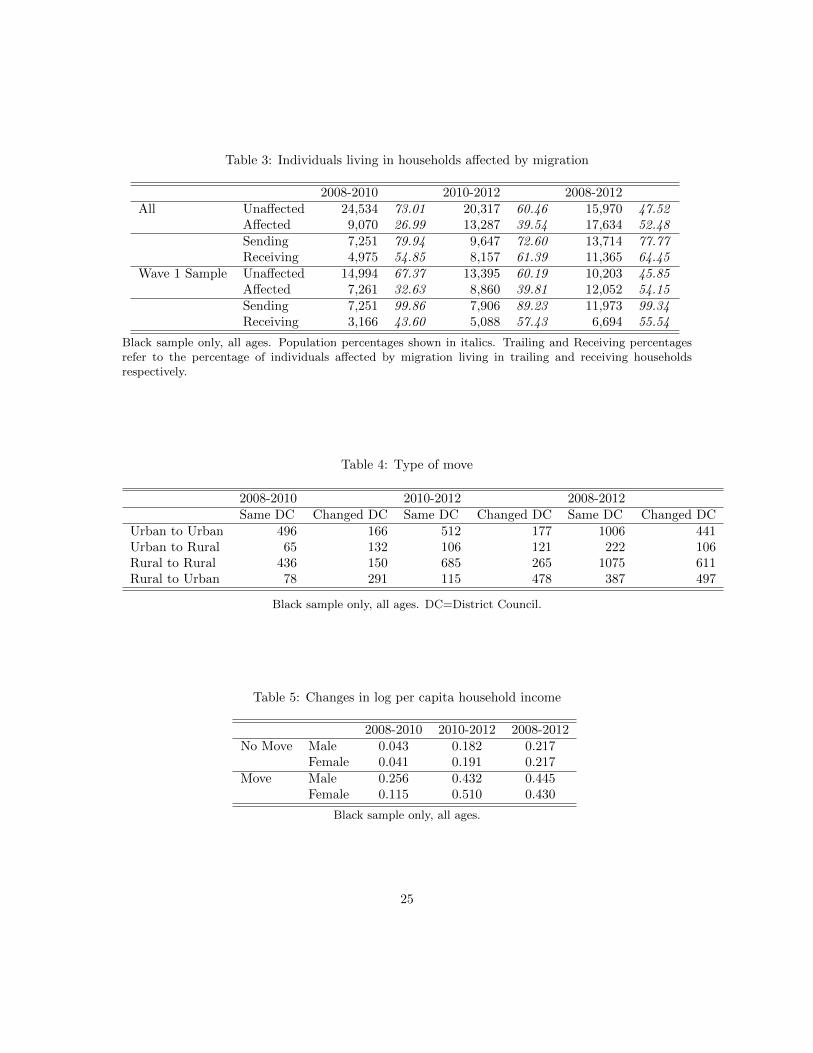
Table 3: Individuals living in households affected by migration

2008-2010 2010-2012 2008-2012All Unaffected 24,534 73.01 20,317 60.46 15,970 47.52

Affected 9,070 26.99 13,287 39.54 17,634 52.48Sending 7,251 79.94 9,647 72.60 13,714 77.77Receiving 4,975 54.85 8,157 61.39 11,365 64.45

Wave 1 Sample Unaffected 14,994 67.37 13,395 60.19 10,203 45.85Affected 7,261 32.63 8,860 39.81 12,052 54.15Sending 7,251 99.86 7,906 89.23 11,973 99.34Receiving 3,166 43.60 5,088 57.43 6,694 55.54

Black sample only, all ages. Population percentages shown in italics. Trailing and Receiving percentagesrefer to the percentage of individuals affected by migration living in trailing and receiving householdsrespectively.

Table 4: Type of move

2008-2010 2010-2012 2008-2012Same DC Changed DC Same DC Changed DC Same DC Changed DC

Urban to Urban 496 166 512 177 1006 441Urban to Rural 65 132 106 121 222 106Rural to Rural 436 150 685 265 1075 611Rural to Urban 78 291 115 478 387 497

Black sample only, all ages. DC=District Council.

Table 5: Changes in log per capita household income

2008-2010 2010-2012 2008-2012No Move Male 0.043 0.182 0.217

Female 0.041 0.191 0.217Move Male 0.256 0.432 0.445

Female 0.115 0.510 0.430

Black sample only, all ages.

25

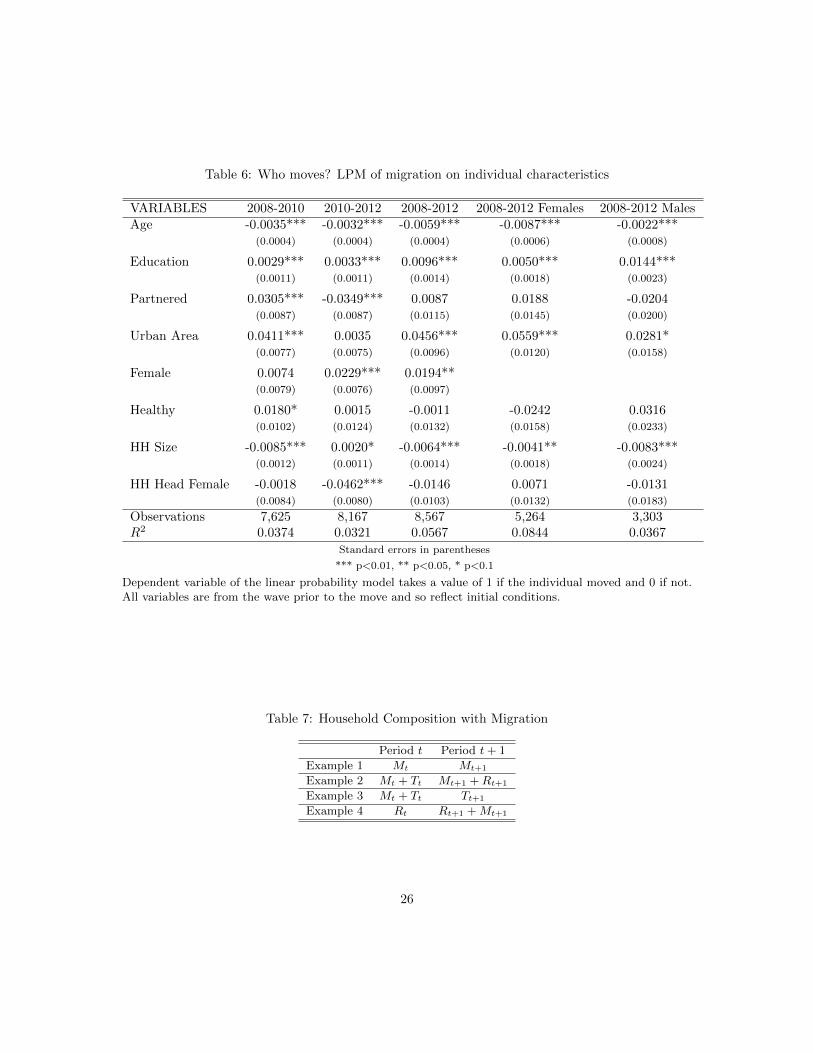
Table 6: Who moves? LPM of migration on individual characteristics

VARIABLES 2008-2010 2010-2012 2008-2012 2008-2012 Females 2008-2012 MalesAge -0.0035*** -0.0032*** -0.0059*** -0.0087*** -0.0022***

(0.0004) (0.0004) (0.0004) (0.0006) (0.0008)

Education 0.0029*** 0.0033*** 0.0096*** 0.0050*** 0.0144***(0.0011) (0.0011) (0.0014) (0.0018) (0.0023)

Partnered 0.0305*** -0.0349*** 0.0087 0.0188 -0.0204(0.0087) (0.0087) (0.0115) (0.0145) (0.0200)

Urban Area 0.0411*** 0.0035 0.0456*** 0.0559*** 0.0281*(0.0077) (0.0075) (0.0096) (0.0120) (0.0158)

Female 0.0074 0.0229*** 0.0194**(0.0079) (0.0076) (0.0097)

Healthy 0.0180* 0.0015 -0.0011 -0.0242 0.0316(0.0102) (0.0124) (0.0132) (0.0158) (0.0233)

HH Size -0.0085*** 0.0020* -0.0064*** -0.0041** -0.0083***(0.0012) (0.0011) (0.0014) (0.0018) (0.0024)

HH Head Female -0.0018 -0.0462*** -0.0146 0.0071 -0.0131(0.0084) (0.0080) (0.0103) (0.0132) (0.0183)

Observations 7,625 8,167 8,567 5,264 3,303R2 0.0374 0.0321 0.0567 0.0844 0.0367

Standard errors in parentheses

*** p<0.01, ** p<0.05, * p<0.1

Dependent variable of the linear probability model takes a value of 1 if the individual moved and 0 if not.All variables are from the wave prior to the move and so reflect initial conditions.

Table 7: Household Composition with Migration

Period t Period t + 1

Example 1 Mt Mt+1

Example 2 Mt + Tt Mt+1 + Rt+1

Example 3 Mt + Tt Tt+1

Example 4 Rt Rt+1 + Mt+1

26

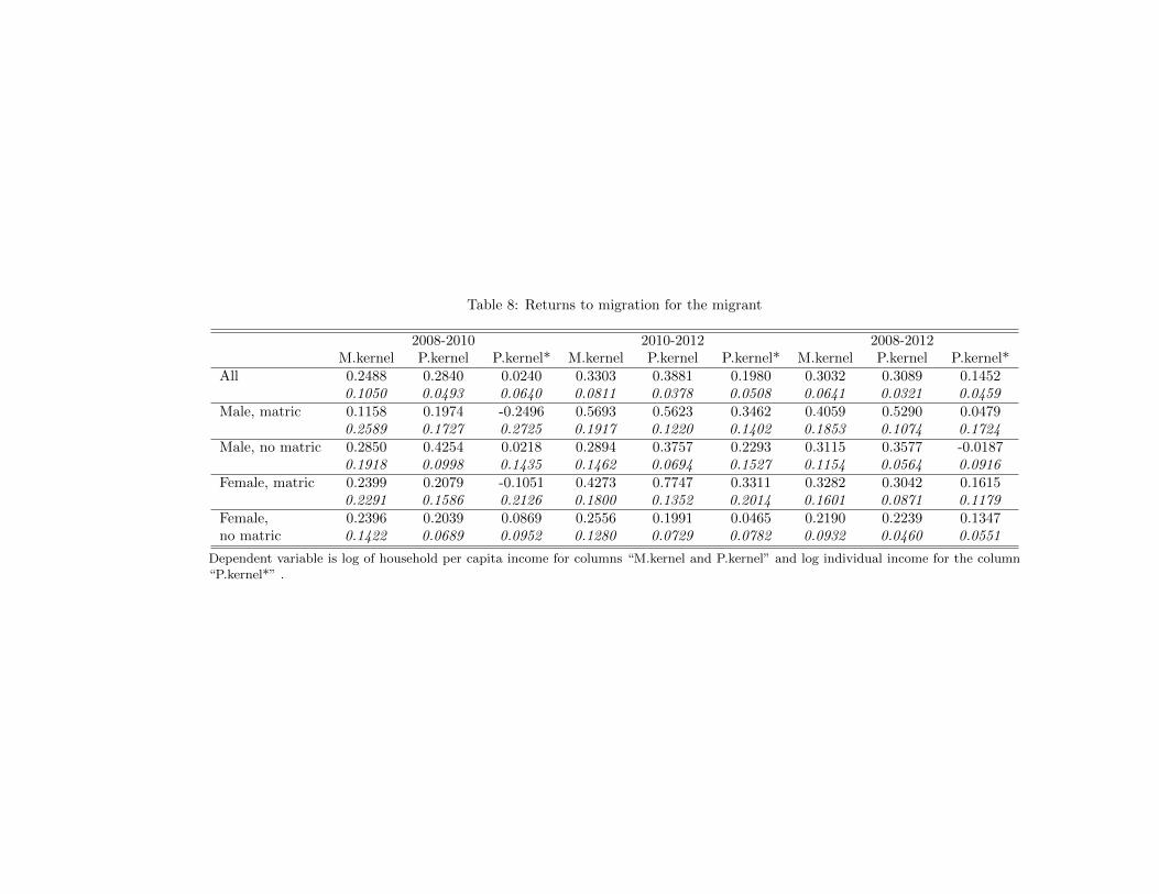
Table 8: Returns to migration for the migrant

2008-2010 2010-2012 2008-2012M.kernel P.kernel P.kernel* M.kernel P.kernel P.kernel* M.kernel P.kernel P.kernel*

All 0.2488 0.2840 0.0240 0.3303 0.3881 0.1980 0.3032 0.3089 0.14520.1050 0.0493 0.0640 0.0811 0.0378 0.0508 0.0641 0.0321 0.0459

Male, matric 0.1158 0.1974 -0.2496 0.5693 0.5623 0.3462 0.4059 0.5290 0.04790.2589 0.1727 0.2725 0.1917 0.1220 0.1402 0.1853 0.1074 0.1724

Male, no matric 0.2850 0.4254 0.0218 0.2894 0.3757 0.2293 0.3115 0.3577 -0.01870.1918 0.0998 0.1435 0.1462 0.0694 0.1527 0.1154 0.0564 0.0916

Female, matric 0.2399 0.2079 -0.1051 0.4273 0.7747 0.3311 0.3282 0.3042 0.16150.2291 0.1586 0.2126 0.1800 0.1352 0.2014 0.1601 0.0871 0.1179

Female, 0.2396 0.2039 0.0869 0.2556 0.1991 0.0465 0.2190 0.2239 0.1347no matric 0.1422 0.0689 0.0952 0.1280 0.0729 0.0782 0.0932 0.0460 0.0551

Dependent variable is log of household per capita income for columns “M.kernel and P.kernel” and log individual income for the column“P.kernel*” .

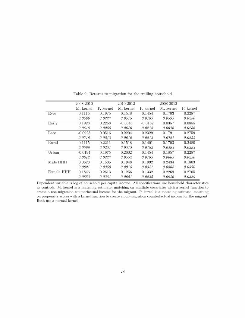
Table 9: Returns to migration for the trailing household

2008-2010 2010-2012 2008-2012M. kernel P. kernel M. kernel P. kernel M. kernel P. kernel

Ever 0.1115 0.1975 0.1518 0.1454 0.1703 0.22870.0566 0.0227 0.0515 0.0183 0.0593 0.0250

Early 0.1928 0.2268 -0.0546 -0.0162 0.0357 0.08550.0618 0.0255 0.0646 0.0218 0.0676 0.0256

Late -0.0923 0.0516 0.2204 0.2329 0.1791 0.27590.0716 0.0243 0.0610 0.0213 0.0721 0.0254

Rural 0.1115 0.2211 0.1518 0.1401 0.1703 0.24800.0566 0.0251 0.0515 0.0182 0.0593 0.0293

Urban -0.0194 0.1975 0.2002 0.1454 0.1857 0.22870.0642 0.0227 0.0552 0.0183 0.0663 0.0250

Male HHH 0.0623 0.1535 0.1948 0.1992 0.2434 0.18030.0821 0.0358 0.0915 0.0341 0.0868 0.0370

Female HHH 0.1846 0.2613 0.1256 0.1332 0.2269 0.27050.0853 0.0381 0.0651 0.0235 0.0946 0.0389

Dependent variable is log of household per capita income. All specifications use household characteristicsas controls. M. kernel is a matching estimate, matching on multiple covariates with a kernel function tocreate a non-migration counterfactual income for the migrant. P. kernel is a matching estimate, matchingon propensity scores with a kernel function to create a non-migration counterfactual income for the migrant.Both use a normal kernel.

28

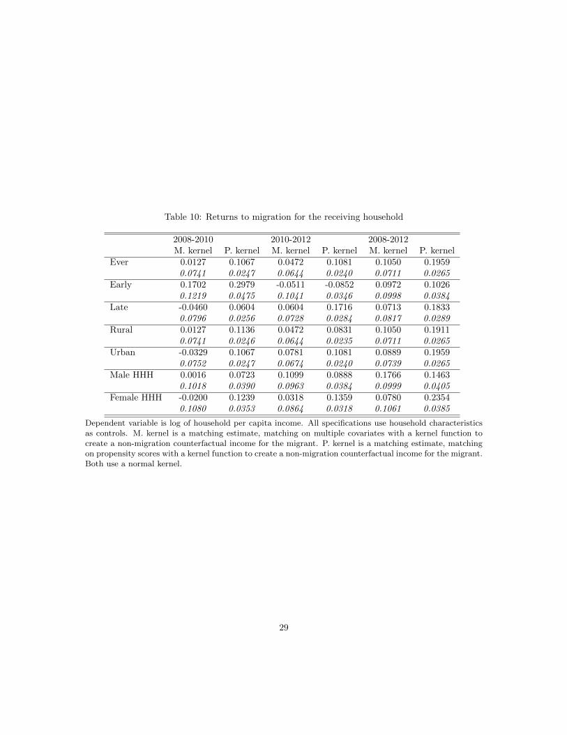
Table 10: Returns to migration for the receiving household

2008-2010 2010-2012 2008-2012M. kernel P. kernel M. kernel P. kernel M. kernel P. kernel

Ever 0.0127 0.1067 0.0472 0.1081 0.1050 0.19590.0741 0.0247 0.0644 0.0240 0.0711 0.0265

Early 0.1702 0.2979 -0.0511 -0.0852 0.0972 0.10260.1219 0.0475 0.1041 0.0346 0.0998 0.0384

Late -0.0460 0.0604 0.0604 0.1716 0.0713 0.18330.0796 0.0256 0.0728 0.0284 0.0817 0.0289

Rural 0.0127 0.1136 0.0472 0.0831 0.1050 0.19110.0741 0.0246 0.0644 0.0235 0.0711 0.0265

Urban -0.0329 0.1067 0.0781 0.1081 0.0889 0.19590.0752 0.0247 0.0674 0.0240 0.0739 0.0265

Male HHH 0.0016 0.0723 0.1099 0.0888 0.1766 0.14630.1018 0.0390 0.0963 0.0384 0.0999 0.0405

Female HHH -0.0200 0.1239 0.0318 0.1359 0.0780 0.23540.1080 0.0353 0.0864 0.0318 0.1061 0.0385

Dependent variable is log of household per capita income. All specifications use household characteristicsas controls. M. kernel is a matching estimate, matching on multiple covariates with a kernel function tocreate a non-migration counterfactual income for the migrant. P. kernel is a matching estimate, matchingon propensity scores with a kernel function to create a non-migration counterfactual income for the migrant.Both use a normal kernel.

29

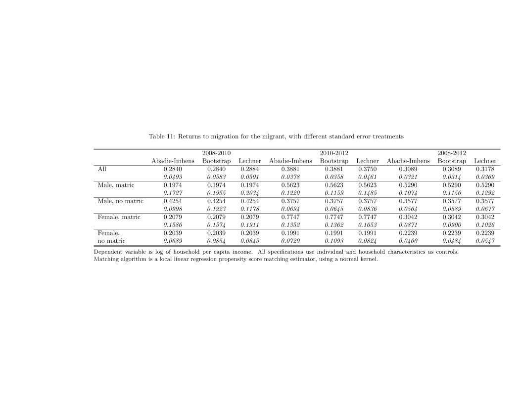
Table 11: Returns to migration for the migrant, with different standard error treatments

2008-2010 2010-2012 2008-2012Abadie-Imbens Bootstrap Lechner Abadie-Imbens Bootstrap Lechner Abadie-Imbens Bootstrap Lechner

All 0.2840 0.2840 0.2884 0.3881 0.3881 0.3750 0.3089 0.3089 0.31780.0493 0.0583 0.0591 0.0378 0.0358 0.0461 0.0321 0.0314 0.0369

Male, matric 0.1974 0.1974 0.1974 0.5623 0.5623 0.5623 0.5290 0.5290 0.52900.1727 0.1955 0.2034 0.1220 0.1159 0.1485 0.1074 0.1156 0.1292

Male, no matric 0.4254 0.4254 0.4254 0.3757 0.3757 0.3757 0.3577 0.3577 0.35770.0998 0.1223 0.1178 0.0694 0.0645 0.0836 0.0564 0.0589 0.0677

Female, matric 0.2079 0.2079 0.2079 0.7747 0.7747 0.7747 0.3042 0.3042 0.30420.1586 0.1574 0.1911 0.1352 0.1362 0.1653 0.0871 0.0900 0.1026

Female, 0.2039 0.2039 0.2039 0.1991 0.1991 0.1991 0.2239 0.2239 0.2239no matric 0.0689 0.0854 0.0845 0.0729 0.1093 0.0824 0.0460 0.0484 0.0547

Dependent variable is log of household per capita income. All specifications use individual and household characteristics as controls.Matching algorithm is a local linear regression propensity score matching estimator, using a normal kernel.

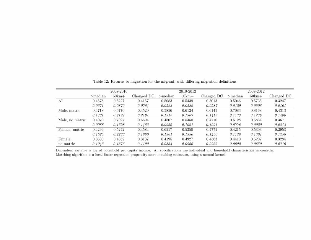
Table 12: Returns to migration for the migrant, with differing migration definitions

2008-2010 2010-2012 2008-2012>median 50km+ Changed DC >median 50km+ Changed DC >median 50km+ Changed DC

All 0.4578 0.5227 0.4157 0.5083 0.5439 0.5013 0.5046 0.5735 0.32470.0671 0.0870 0.0764 0.0523 0.0589 0.0587 0.0429 0.0508 0.0464

Male, matric 0.4718 0.6776 0.4520 0.5856 0.6124 0.6145 0.7083 0.8168 0.43130.1731 0.2197 0.2194 0.1315 0.1367 0.1413 0.1173 0.1276 0.1406

Male, no matric 0.4070 0.7027 0.5694 0.4807 0.5350 0.4710 0.5128 0.5834 0.36710.0988 0.1698 0.1453 0.0966 0.1091 0.1091 0.0776 0.0920 0.0813

Female, matric 0.4299 0.5242 0.4584 0.6517 0.5350 0.4771 0.4215 0.5303 0.29530.1625 0.2233 0.1880 0.1361 0.1556 0.1450 0.1128 0.1304 0.1258

Female, 0.3330 0.4052 0.3137 0.4195 0.4927 0.4563 0.4410 0.5207 0.3284no matric 0.1043 0.1376 0.1190 0.0834 0.0966 0.0966 0.0692 0.0850 0.0716

Dependent variable is log of household per capita income. All specifications use individual and household characteristics as controls.Matching algorithm is a local linear regression propensity score matching estimator, using a normal kernel.

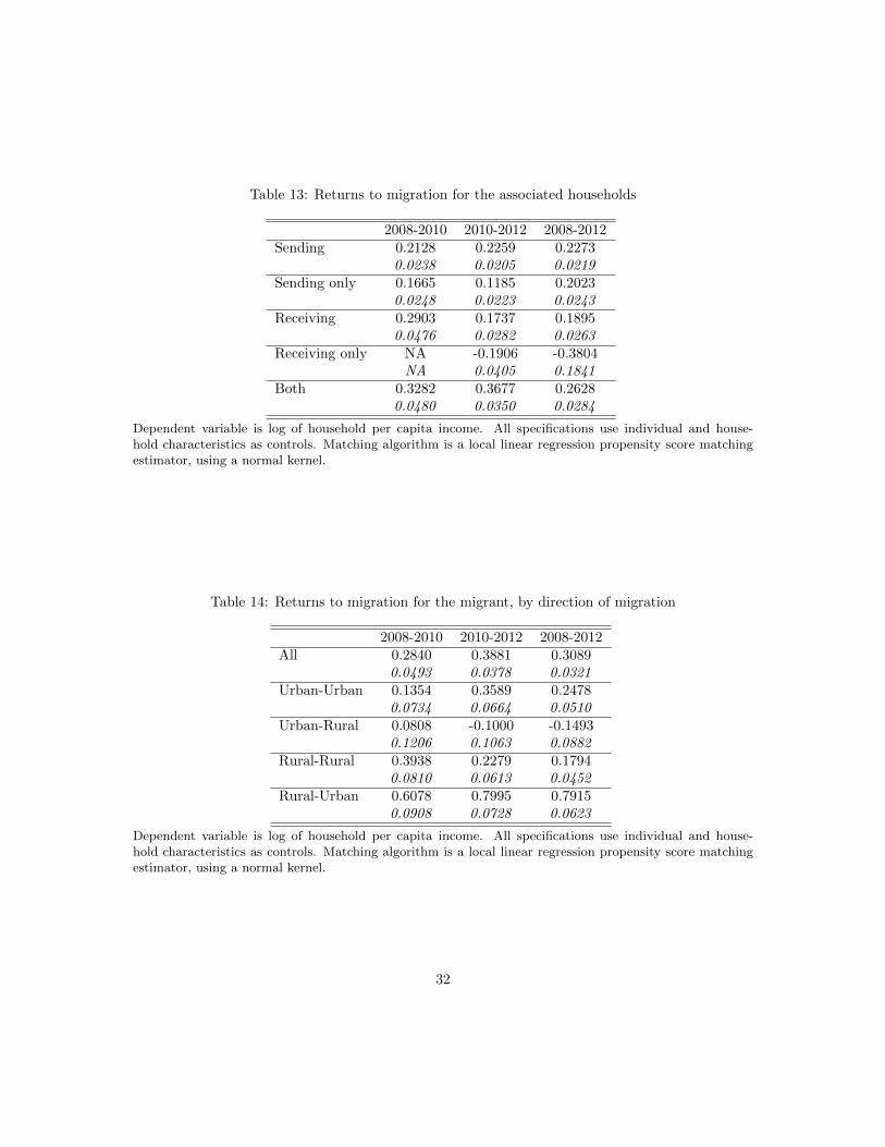
Table 13: Returns to migration for the associated households

2008-2010 2010-2012 2008-2012Sending 0.2128 0.2259 0.2273

0.0238 0.0205 0.0219Sending only 0.1665 0.1185 0.2023

0.0248 0.0223 0.0243Receiving 0.2903 0.1737 0.1895

0.0476 0.0282 0.0263Receiving only NA -0.1906 -0.3804

NA 0.0405 0.1841Both 0.3282 0.3677 0.2628

0.0480 0.0350 0.0284

Dependent variable is log of household per capita income. All specifications use individual and house-hold characteristics as controls. Matching algorithm is a local linear regression propensity score matchingestimator, using a normal kernel.

Table 14: Returns to migration for the migrant, by direction of migration

2008-2010 2010-2012 2008-2012All 0.2840 0.3881 0.3089

0.0493 0.0378 0.0321Urban-Urban 0.1354 0.3589 0.2478

0.0734 0.0664 0.0510Urban-Rural 0.0808 -0.1000 -0.1493

0.1206 0.1063 0.0882Rural-Rural 0.3938 0.2279 0.1794

0.0810 0.0613 0.0452Rural-Urban 0.6078 0.7995 0.7915

0.0908 0.0728 0.0623

Dependent variable is log of household per capita income. All specifications use individual and house-hold characteristics as controls. Matching algorithm is a local linear regression propensity score matchingestimator, using a normal kernel.

32

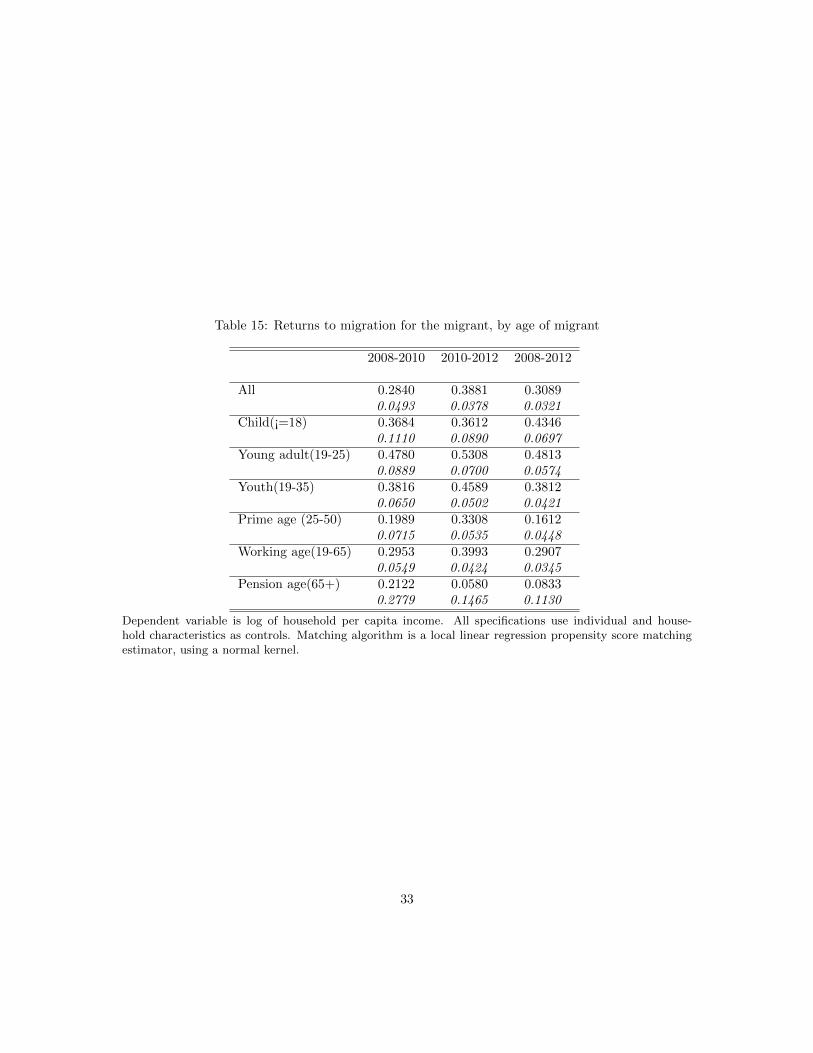
Table 15: Returns to migration for the migrant, by age of migrant

2008-2010 2010-2012 2008-2012

All 0.2840 0.3881 0.30890.0493 0.0378 0.0321

Child(¡=18) 0.3684 0.3612 0.43460.1110 0.0890 0.0697

Young adult(19-25) 0.4780 0.5308 0.48130.0889 0.0700 0.0574

Youth(19-35) 0.3816 0.4589 0.38120.0650 0.0502 0.0421

Prime age (25-50) 0.1989 0.3308 0.16120.0715 0.0535 0.0448

Working age(19-65) 0.2953 0.3993 0.29070.0549 0.0424 0.0345

Pension age(65+) 0.2122 0.0580 0.08330.2779 0.1465 0.1130

Dependent variable is log of household per capita income. All specifications use individual and house-hold characteristics as controls. Matching algorithm is a local linear regression propensity score matchingestimator, using a normal kernel.

33