Draft Modeling Protocol

Procedures for Modeling 8-Hour Ozone Concentrations in the Baton Rouge 5-Parish Area

Prepared by

Air Quality Assessment Division Office of Environmental Assessment

Louisiana Department of Environmental Quality 602 North Fifth Street

Baton Rouge, Louisiana 70802

15 September 2006 P.O. Box 4314, Baton Rouge, LA 70821-4314 225.219.3288

i

TABLE OF CONTENTS

Page 1.0 INTRODUCTION.......................................................................................................... 1-1

1.1 Overview.................................................................................................................... 1-1 1.2 Study Background...................................................................................................... 1-1 1.3 Lead Agency and Principal Participants .................................................................... 1-2 1.4 Related Regional Modeling Studies........................................................................... 1-2

1.4.1 Related Regional Regulatory Air Quality Studies ............................................... 1-2 1.4.2 Related Local Air Quality Planning Efforts......................................................... 1-3 1.4.3 PM2.5 and Regional Haze SIP Studies................................................................ 1-5

1.5 Overview of Modeling Approach .............................................................................. 1-6 1.5.1 Ozone Episode Selection ..................................................................................... 1-6

1.5.1.1 EPA Guidance for Episode Selection ........................................................... 1-6 1.5.1.2 Selection of Baton Rouge Ozone Modeling Episodes.................................. 1-7

1.5.2 Model Selection ................................................................................................... 1-7 1.5.3 Emissions Input Preparation and QA/QC............................................................ 1-8 1.5.4 Meteorology Input Preparation and QA/QC........................................................ 1-9 1.5.5 Air Quality Modeling Input Preparation and QA/QC........................................ 1-10 1.5.6 Proposed Model Performance Goals ................................................................. 1-11 1.5.7 Diagnostic and Sensitivity Studies..................................................................... 1-11

1.5.7.1 Traditional Sensitivity Testing.................................................................... 1-11 1.5.7.2 Diagnostic Tests.......................................................................................... 1-13

1.5.8 Weight of Evidence Analyses ............................................................................ 1-14 1.5.9 Assessing Model Reliability in Estimating the Effects of Emissions Changes . 1-15 1.5.10 Future Year Control Strategy Modeling ............................................................ 1-16 1.5.11 Future Year Ozone Attainment Demonstration ................................................. 1-16

1.6 Project Participants and Contacts............................................................................. 1-16 1.7 Communication........................................................................................................ 1-17 1.8 Preliminary Modeling Protocol and Response to EPA Comments ......................... 1-17

2.0 MODEL SELECTION .................................................................................................. 2-1

2.1 Regulatory Context for Model Selection ................................................................... 2-1

2.1.1 Summary of Recommended Models .................................................................... 2-2 2.2 Details of the Recommended Models ........................................................................ 2-3

2.2.1 The MM5 Meteorological Model......................................................................... 2-3 2.2.2 The EPS3 Emissions Modeling System .............................................................. 2-4 2.2.3 The CAMx Regional Photochemical Model........................................................ 2-5

2.3 Justification for Model Selection............................................................................... 2-7 2.3.1 MM5 .................................................................................................................... 2-7 2.3.2 EPS3 ..................................................................................................................... 2-8 2.3.3 CAMx .................................................................................................................. 2-8

2.4 Model Limitations...................................................................................................... 2-9 2.4.1 MM5..................................................................................................................... 2-9

ii

2.4.2 EPS3 ..................................................................................................................... 2-9 2.4.3 CAMx ................................................................................................................ 2-10

2.5 Model Input Requirements ...................................................................................... 2-10 2.5.1 MM5 .................................................................................................................. 2-11 2.5.2 EPS3 ................................................................................................................... 2-11 2.5.3 CAMx................................................................................................................. 2-11

2.6 Summary of Model Selection and Justification ....................................................... 2-11 2.7 Availability of Model Codes, Analysis Tools and Related Software ...................... 2-12

3.0 EPISODE SELECTION................................................................................................ 3-1

3.1 Overview of EPA Guidance....................................................................................... 3-1 3.1.1 Primary Criteria ................................................................................................... 3-1

3.1.2 Secondary Criteria................................................................................................ 3-1 3.1.3 Methods Commonly Used to Identify Candidate Episode................................... 3-1 3.1.4 Summary of CART Analysis ............................................................................... 3-2

3.2 Selection of Baton Rouge 8-hour Ozone Modeling Episodes ................................... 3-2 3.2.1 Key Baton Rouge Ozone Monitors ...................................................................... 3-3 3.2.2 Episode Selection Approach ................................................................................ 3-3 3.2.3 Prioritization of Candidate Modeling Episodes ................................................... 3-7 3.2.4 Further Analysis of Five Candidate Episodes...................................................... 3-9

3.3 Conceptual Model and Aerometric Conditions of each Episode............................. 3-11 3.3.1 May 22-28, 2005 ................................................................................................ 3-12 3.3.2 May 19-30, 2003 ................................................................................................ 3-14 3.3.3 September 28-30, 2004 ...................................................................................... 3-21 3.3.4 April 12-30, 2003 ............................................................................................... 3-25 3.3.5 October 4-6, 2003............................................................................................... 3-30 3.3.6 May 4-9, 2004 .................................................................................................... 3-34 3.3.7 August 11 – September 5, 2000 ......................................................................... 3-38

4.0 MODELING DOMAINS AND DATA AVAILABILITY.......................................... 4-1

4.1 Horizontal Modeling Domain .................................................................................... 4-1 4.2 Vertical Modeling Domain ........................................................................................ 4-4 4.3 Data Availability........................................................................................................ 4-6

4.3.1 Emissions Data..................................................................................................... 4-6 4.3.2 Air Quality............................................................................................................ 4-6 4.3.3 Ozone Column Data ............................................................................................. 4-6 4.3.4 Meteorological Data............................................................................................. 4-8 4.3.5 Initial and Boundary Conditions Data.................................................................. 4-8

5.0 MODEL INPUT PREPARATION PROCEDURES .................................................. 5-1 5.1 Meteorological Inputs ................................................................................................ 5-1

5.1.1 MM5 Model Science Configuration ................................................................... 5-1 5.1.2 MM5 Input Data Preparation Procedures ............................................................ 5-1 5.1.3 MM5CAMx Reformatting Methodology ............................................................ 5-3

iii

5.1.4 Treatment of Minimum KV................................................................................. 5-4 5.2 Emission Inputs.......................................................................................................... 5-4

5.2.1 Available Emissions Inventory Datasets ............................................................. 5-4 5.2.2 Development of CAMx-Ready Episodic Emissions Inventories......................... 5-5 5.2.2.1 Episodic On-Road Mobile Source Emissions............................................... 5-7 5.2.2.2 Episodic Biogenic Source Emissions............................................................ 5-8

5.2.2.3 Point Source Emissions ................................................................................ 5-8 5.2.2.4 Area and Non-Road Source Emissions......................................................... 5-8 5.2.2.5 Wildfires, Prescribed Burns, Agricultural Burns.......................................... 5-8 5.2.2.6 QA/QC and Emissions Merging ................................................................... 5-8 5.2.3 Use of the Plume-in-Grid (PiG) Subgrid-Scale Plume Treatment....................... 5-9 5.2.4 Products of the Emissions Inventory Development Process.............................. 5-10 5.2.5 Future-Year Emissions Modeling ...................................................................... 5-11 5.3 Photochemical Modeling Inputs .............................................................................. 5-11 5.3.1 CAMx Science Configuration and Input Configuration.................................... 5-11 6.0 OZONE MODEL PERFORMANCE EVALUATION .............................................. 6-1 6.1 Establishing Base Case CAMx Simulations for Baton Rouge Episodes................... 6-1 6.1.1 Setting Up and Exercising CAMx Base Cases .................................................... 6-1 6.1.2 Use of Sensitivity, Source Apportionment, and Related Diagnostic Probing Tools .................................................................................... 6-2 6.2 Evaluation of CAMx Base Cases for the Baton Rouge Episodes.............................. 6-3 6.2.1 Overview.............................................................................................................. 6-3 6.2.2 Meteorological Model Evaluation Methodology................................................. 6-5 6.2.2.1 Components of the Baton Rouge MM5 Evaluation...................................... 6-5 6.2.2.2 Data Supporting Model Evaluation ............................................................ 6-5 6.2.2.3 Evaluation Tools ........................................................................................... 6-6 6.2.3 Photochemical Model Evaluation Methodology ................................................. 6-6 6.2.4 Available Aerometric Data for the Evaluations................................................... 6-9 7.0 FUTURE YEAR MODELING ..................................................................................... 7-1 7.1 Future Year to be Simulated ...................................................................................... 7-1 7.2 Future Year Growth and Controls.............................................................................. 7-1 7.2.1 Regional Growth and Control Factors ................................................................. 7-2 7.2.2 Local Growth and Control Factors....................................................................... 7-2 7.3 Future Model–Ready Emissions Inventory Development and QA ........................... 7-2 7.4 Future Year Baseline Air Quality Simulations .......................................................... 7-3 7.4.1 Future-Year Initial and Boundary Conditions ..................................................... 7-3 7.4.2 Other Future-Year Modeling Inputs .................................................................... 7-3 7.5 Emissions Sensitivity Experiments............................................................................ 7-3 7.6 Control Strategy Development, Testing and Analysis............................................... 7-4

iv

8.0 OZONE ATTAINMENT DEMONSTRATION ......................................................... 8-1 8.1 Ozone Weight of Evidence Analyses .......................................................................8-1 8.2 8-Hour Ozone Attainment Demonstration Procedures .............................................8-1 REFERENCES.......................................................................................................................... R-1

APPENDICES Appendix A: Quality Assurance Project Plan Appendix B: Daily Maximum 8-Hour Ozone Concentrations (ppb) in the Baton Rouge 5-Parish Area for 2000 - 2005 Appendix C: 48-Hour Backward Trajectories Ending in Baton Rouge

On the Afternoon of Each 8-hour Ozone Exceedance Day of the Six Candidate Episodes (Chapter 3)

TABLES

Table 2-1. Factors Qualifying MM5 for Use in the Baton Rouge Ozone Modeling Study ...................................................................................... 2-13 Table 2-2. Factors Qualifying EPS for Use in the Baton Rouge Ozone Modeling Study ...................................................................................... 2-14 Table 2-3. Factors Qualifying CAMx for Use in the Baton Rouge Ozone Modeling Study ...................................................................................... 2-15 Table 2-4. Factors Justifying MM5 as the Meteorological Model for the Baton Rouge Ozone Modeling Study .......................................................... 2-16 Table 2-5. Factors Justifying EPS3 as the Emissions Model for the Baton Rouge Ozone Modeling Study ................................................................ 2-17 Table 2-6. Factors Justifying CAMx as a Photochemical Model for the Baton Rouge Ozone Modeling Study ................................................................ 2-18 Table 3-1. 8-hour ozone Design Values for the years 1998-2005 and fourth highest 8-hour ozone concentrations for 1998-2002 at monitors in the Baton Rouge 5-Parish area. .................................................... 3-4 Table 3-2. Summary of candidate 8-hour ozone modeling episodes from 2000-2005 for the Baton Rouge 5-Parish area............................................ 3-6 Table 3-3. Observed 8-hour ozone Design Values and peak 8-hour ozone concentrations (ppb) for the candidate 8-hour ozone episodes for the Baton Rouge area....................................................................... 3-8 Table 3-4. Number of days daily maximum 8-hour ozone concentrations was 70 ppb or higher at each Baton Rouge monitor and for the candidate 8-hour ozone episodes ......................................................................... 3-8 Table 3-5a. Number of observed ozone days > 70 ppb for the top six ranked candidate episode and total days across highest ranked episodes...................... 3-10 Table 3-5b. Number of observed ozone days > 85 ppb for the top six ranked candidate episode and total days across highest ranked episodes. ..................... 3-10

v

Table 3-6. CART Bins for 4 ranked episodes for which data are available (Source: ICF, 2005)............................................................................................ 3-11 Table 4-1. Lambert Conformal Projection (LCP) definition for the Baton Rouge 36/12/4 km modeling grid.............................................................. 4-4 Table 4-2. Grid definitions for MM5, EPS and CAMx......................................................... 4-4 Table 4-3. Vertical Layer Definition for MM5 Simulations (left most columns), and Approach for Reducing CAMx Layers by Collapsing Multiple MM5 layers (right columns) ................................................................. 4-5 Table 4-4. Overview of ambient data monitoring networks. The EPA AQS/AIRS and PAMS networks. ........................................................................................... 4-7 Table 5-1. MM5 (Version 3.7) model configuration............................................................. 5-2 Table 5-2. EPS (Version 3) configuration............................................................................. 5-6 Table 5-3. CAMx (Version 4.3 or 4.4) model configuration .............................................. 5-13 Table 6-1. Statistical measures and graphical displays used in the MM5 operational evaluation.................................................................... 6-10 Table 6-2. Statistical measures and graphical displays used in the MM5 scientific evaluation. (measures and displays developed for each simulation day). .................................................... 6-12 Table 6-3. Statistical measures and graphical displays for 1-hour and 8-hour ozone concentrations to be used in the screening model performance evaluation (SMPE) of CAMx surface ozone concentrations. .............................................................. 6-13 Table 6-4. Statistical measures and graphical displays for 1-hour and 8-hour ozone, VOCs, NOx, and indicator species and indicator species Ratios to be used in the refined model performance evaluation (RMPE) involving multi-species, multi-scale evaluation of CAMx surface and aloft concentrations. .................................................................................. 6-14

FIGURES

Figure 3-1 Locations of Baton Rouge ozone monitors.......................................................... 3-4 Figure 3-2a. Hourly ozone (ppb) at the four key Baton Rouge monitors: LSU (BR), Baker (BK), Carville (CV), and Port Allen (PA). ........................... 3-13 Figure 3-2b. Hourly ozone (ppb) at the other Baton Rouge monitors: Capitol (BC), Pride (PE), Bayou Plaquemine (BP), Grosse Tete (GT), Dutchtown (DT), and French Settlement (FS)......................................... 3-13 Figure 3-3a. Average, maximum, and minimum hourly wind speed (mph) among the Baton Rouge monitors........................................................... 3-15 Figure 3-3b. Average, maximum, and minimum hourly temperature (C) among the Baton Rouge monitors ............................................................... 3-15 Figure 3-4. Wind rose based on hourly wind speed/direction data from all Baton Rouge monitors between 6 AM and 6 PM on exceedance days ........ 3-16 Figure 3-5a. Hourly ozone (ppb) at the four key Baton Rouge monitors: LSU (BR), Baker (BK), Carville (CV), and Port Allen (PA). ........................... 3-17

vi

Figure 3-5b. Hourly ozone (ppb) at the other Baton Rouge monitors: Capitol (BC), Pride (PE), Bayou Plaquemine (BP), Grosse Tete (GT), Dutchtown (DT), and French Settlement (FS)......................................... 3-17 Figure 3-6a. Average, maximum, and minimum hourly wind speed (mph) among the Baton Rouge monitors. The extreme winds on May 30 are likely erroneous .............................................................................. 3-19 Figure 3-6b. Average, maximum, and minimum hourly temperature (C) among the Baton Rouge monitors ............................................................... 3-19 Figure 3-7. Wind rose based on hourly wind speed/direction data from all Baton Rouge monitors between 6 AM and 6 PM on exceedance days ........ 3-20 Figure 3-8a. Hourly ozone (ppb) at the four key Baton Rouge monitors: LSU (BR), Baker (BK), Carville (CV), and Port Allen (PA). ........................... 3-22 Figure 3-8b. Hourly ozone (ppb) at the other Baton Rouge monitors: Capitol (BC), Pride (PE), Bayou Plaquemine (BP), Grosse Tete (GT), Dutchtown (DT), and French Settlement (FS)......................................... 3-22 Figure 3-9a. Average, maximum, and minimum hourly wind speed (mph) among the Baton Rouge monitors........................................................... 3-23 Figure 3-9b. Average, maximum, and minimum hourly temperature (C) among the Baton Rouge monitors ............................................................... 3-23 Figure 3-10. Wind rose based on hourly wind speed/direction data from all Baton Rouge monitors between 6 AM and 6 PM on exceedance days ........ 3-24 Figure 3-11a. Hourly ozone (ppb) at the four key Baton Rouge monitors: LSU (BR), Baker (BK), Carville (CV), and Port Allen (PA). ........................... 3-26 Figure 3-11b. Hourly ozone (ppb) at the other Baton Rouge monitors: Capitol (BC), Pride (PE), Bayou Plaquemine (BP), Grosse Tete (GT), Dutchtown (DT), and French Settlement (FS)................................. 3-26 Figure 3-12a. Average, maximum, and minimum hourly wind speed (mph) among the Baton Rouge monitors........................................................... 3-28 Figure 3-12b. Average, maximum, and minimum hourly temperature (C) among the Baton Rouge monitors. .............................................................. 3-28 Figure 3-13. Wind rose based on hourly wind speed/direction data from all Baton Rouge monitors between 6 AM and 6 PM on exceedance days ........ 3-29 Figure 3-14a. Hourly ozone (ppb) at the four key Baton Rouge monitors: LSU (BR), Baker (BK), Carville (CV), and Port Allen (PA) ............................ 3-31 Figure 3-14b. Hourly ozone (ppb) at the other Baton Rouge monitors: Capitol (BC), Pride (PE), Bayou Plaquemine (BP), Grosse Tete (GT), Dutchtown (DT), and French Settlement (FS)......................................... 3-31 Figure 3-15a. Average, maximum, and minimum hourly wind speed (mph) among the Baton Rouge monitors........................................................... 3-32 Figure 3-15b. Average, maximum, and minimum hourly temperature (C) among the Baton Rouge monitors ............................................................... 3-32 Figure 3-16. Wind rose based on hourly wind speed/direction data from all Baton Rouge monitors between 6 AM and 6 PM on exceedance days ........ 3-33 Figure 3-17a. Hourly ozone (ppb) at the four key Baton Rouge monitors: LSU (BR), Baker (BK), Carville (CV), and Port Allen (PA). ........................... 3-35

vii

Figure 3-17b. Hourly ozone (ppb) at the other Baton Rouge monitors: Capitol (BC), Pride (PE), Bayou Plaquemine (BP), Grosse Tete (GT), Dutchtown (DT), and French Settlement (FS)................................. 3-35 Figure 3-18a. Average, maximum, and minimum hourly wind speed (mph) among the Baton Rouge monitors........................................................... 3-36 Figure 3-18b. Average, maximum, and minimum hourly temperature (C) among the Baton Rouge monitors ............................................................... 3-36 Figure 3-19. Wind rose based on hourly wind speed/direction data from all Baton Rouge monitors between 6 AM and 6 PM on exceedance days ........ 3-37 Figure 3-20a. Hourly ozone (ppb) at the four key Baton Rouge monitors: LSU (BR), Baker (BK), Carville (CV), and Port Allen (PA). ........................... 3-39 Figure 3-20b. Hourly ozone (ppb) at the other Baton Rouge monitors: Capitol (BC), Pride (PE), Bayou Plaquemine (BP), Grosse Tete (GT), Dutchtown (DT), and French Settlement (FS)......................................... 3-39 Figure 3-21a. Average, maximum, and minimum hourly wind speed (mph) among the Baton Rouge monitors...................................................................... 3-40 Figure 3-21b. Average, maximum, and minimum hourly temperature (C) among the Baton Rouge monitors...................................................................... 3-40 Figure 3-22. Wind rose based on hourly wind speed/direction data from all Baton Rouge monitors between 6 AM and 6 PM on exceedance days. ....... 3-41 Figure 4-1a. Nested 36/12/4 km modeling domains for the Baton Rouge 8-hour ozone modeling study. Dotted line domains are for CAMx/EPS that are nested in the MM5 solid line domains ................................................................................................ 4-2 Figure 4-1b. Nested 12/4 km modeling domains for the Baton Rouge 8-hour ozone modeling study. Dotted line domains are for CAMx/EPS that are nested in the MM5 solid line domains .......................... 4-3 Figure 4-1c. 4 km Louisiana modeling domain for the Baton Rouge 8-hour ozone modeling study. Red dotted line domain is for CAMx/EPS that are nested in the MM5 domain............................................ 4-3

1-1

1.0 INTRODUCTION 1.1 Overview

This report constitutes the Air Quality Modeling Protocol for the Baton Rouge 5-Parish 8-hour ozone modeling analysis in support of 8-hour ozone attainment demonstration modeling of the Baton Rouge area. It describes the overall modeling activities to be performed by the Louisiana Department of Environmental Quality (LDEQ) in order to demonstrate attainment of the 8-hour ozone standard in Baton Rouge and other areas in Louisiana.

A comprehensive modeling protocol for an 8-hour ozone SIP attainment demonstration study consists of many elements. Its main function is to serve as a means for planning and communicating how a modeled attainment demonstration will be performed before it occurs. The protocol guides the technical details of a modeling study and provides a formal framework within which the scientific assumptions, operational details, commitments and expectations of the various participants can be set forth explicitly and means for resolution of potential differences of technical and policy opinion can be worked out openly and within prescribed time and budget constraints.

As noted in the U.S. Environmental Protection Agency’s (EPA) 8-hour ozone modeling

guidance, the modeling protocol serves several important functions (EPA, 2005a): • Identify the assistance available to the LDEQ (the lead agency) to undertake and

evaluate the analysis needed to support a defensible attainment demonstration; • Identify how communication will occur among States/Tribes and stakeholders to

develop a consensus on various issues; • Describe the review process applied to key steps in the demonstration; and • Describe how changes in methods and procedures or in the protocol itself will be

agreed upon and communicated with stakeholders and the appropriate U.S. EPA regional Office.

1.2 Study Background

The main goal of the Baton Rouge 8-Hour Ozone Attainment Demonstration Study is to develop the photochemical modeling data bases and associated analysis tools needed to reliably simulate the processes responsible for 8-hour ozone exceedances in the Baton Rouge region and the evaluation of realistic emissions reduction strategies for inclusion in the Baton Rouge 8-hour ozone SIP. Based on measured ozone data from 2001-2003, the EPA designated the Baton Rouge 5-Parish area as a Marginal 8-hour ozone nonattainment area. Although EPA does not require a modeled attainment demonstration for Marginal nonattainment areas, the Baton Rouge area has experienced high ozone conditions in 2005 and to date in 2006 and will not attain the 8-hour ozone standard in 2006 to meet the June 15, 2007 attainment date for Marginal areas. The Baton Rouge area will likely face a “bump-up” to the Moderate classification with an attainment date

1-2

of June 15, 2010. With the Moderate classification, a modeled attainment demonstration must be submitted to the EPA. 1.3 Lead Agency and Principal Participants

The Louisiana Department of Environmental Quality (LDEQ) Office of Environmental

Assessment, Air Quality Assessment Division is the lead agency in the development of the Baton Rouge 8-hour ozone SIP. EPA Region 6 in Dallas, Texas is the local regional EPA office that will take the lead in the approval process for the Baton Rouge 8-hour ozone SIP. The LDEQ has contracted with ENVIRON International Corporation to assist them in the 8-hour ozone attainment modeling demonstration. 1.4 Related Regional Modeling Studies

The Baton Rouge 8-hour Ozone Study draws from several urban- and regional scale

emissions, photochemical, PM, and visibility modeling efforts performed in the central states and across the United States. The procedures used in these previous studies provide a guide to the modeling and QA approach for the Baton Rouge study. 1.4.1 Related Regional Regulatory Air Quality Studies

There are several related regulatory air issues that have direct relevance to the Baton Rouge 8-hour ozone attainment demonstration SIP. These issues include, but are not limited to, the following:

Clean Air Interstate Rule (CAIR): The State of Louisiana is part of the CAIR controls for both ozone and PM2.5. EPA determined that Louisiana contributed significantly to downwind 8-hour ozone nonattainment in Galveston, Harris and Jefferson Counties, Texas (EPA. 2005b). EPA also determined that Louisiana also contributed significantly to downwind PM2.5 nonattainment in Jefferson and Russell Counties, Alabama. Accordingly, Louisiana will be subject to the NOx and SO2 emission control requirements under both the ozone and PM2.5 provisions of the CAIR. The CAIR determined which states contributed significantly to downwind PM2.5 and ozone nonattainment using the CMAQ and CAMx models, respectively. Clean Air Mercury Rule (CAMR): Louisiana Electrical Generating Units (EGU) are subject to the requirements of the Clean Air Mercury Rule (CAMR). Clean Air Visibility Rule (CAVR): The Clean Air Visibility Rule (CAVR) requires specific sources that are shown to reasonably contribute to visibility impairment at a Class I area to install Best Available Retrofit Technology (BART). The BART requirements apply to sources built between 1962 and 1977 that have the potential to emit 250 tons per year (TPY) of a visibility impairing pollutants (SO2, NOx, PM and/or VOC) and are one of 26 specific source categories. EPA has published guidelines for the BART component of the CAVR (EPA, 2005c). In November 2002, the LDEQ distributed a survey and based on that survey published a list of potentially BART-eligible sources

1-3

(see: http://www.deq.louisiana.gov/portal/Portals/0/AirQualityAssessment/BART%20eligible%20sources.pdf).

1.4.2 Related Local Air Quality Planning Efforts There are several ozone air quality planning efforts in the central states that are related to

the Baton Rouge 8-hour ozone study, either by their proximity so they may affect transport into the area or they may contain air quality control measures that may be of interest. Below we summarize many of these efforts, including 8-hour ozone Early Action Compact (EAC) State Implementation Plans (SIPs) that were submitted to EPA in December 2004 as well as ongoing 8-hour ozone planning in nearby nonattainment areas.

Houston/Galveston/Brazoria Area (HGB) Ozone Attainment: The HGB has been the subject of several ozone modeling efforts. During summer of 2000 a massive air quality field study was performed (TexAQS2000) that was used to develop a photochemical modeling database from August-September 2000. The Texas Commission on Environmental Quality (TCEQ) is currently developing enhanced ozone modeling databases in preparation for the HGB 8-hour ozone SIP due June 2007. The TCEQ is using the MM5/EPS/CAMx modeling system for their ozone attainment demonstration modeling. Details on the TCEQ HGB ozone modeling activities can be found on their website (see: http://www.tceq.state.tx.us/nav/eq/sip.html). Beaumont/Port-Arthur (BPA) Ozone Attainment: In September 2005, the TCEQ approved adoption of an 8-hour ozone attainment demonstration SIP for the BPA nonattainment area. Ozone nonattainment problems in the Houston and Beaumont areas are linked by their proximity and the complex meteorological patterns along the Gulf Coast. TCEQ uses the same MM5/EPS/CAMx ozone-modeling databases for both BPA and HGB and was able to develop BPA control strategies that demonstrate attainment by 2007. Dallas/Fort-Worth (DFW) Ozone Attainment: The TCEQ is developing an 8-hour ozone SIP for the DFW area (see: http://www.tceq.state.tx.us/implementation/air/sip/dfw.html) and plans to propose the SIP for adoption in late 2006. The DFW SIP will be one of the first 8-hour ozone plans for a major metropolitan area to come before EPA and the TCEQ is working closely with EPA’s regional office and OAQPS to establish the procedures for modeling and attainment demonstrations. TCEQ is using the MM5/EPS/CAMx modeling system for the DFW 8-hour ozone SIP.

St. Louis Ozone Attainment: The Missouri Department of Natural Resources (MDNR) and the Illinois Environmental Projection Agency (IEPA) are jointly developing an 8-hour ozone SIP for the St. Louis region. Link-based on-road mobile source emissions are being developed for the greater St. Louis area, with regional emissions obtained from the CENRAP effort. MDNR/IEPA are using the MM5/SMOKE/CAMx modeling system for the St. Louis 8-hour ozone SIP.

Texas 8-Hour Ozone EAC SIPs: Several of the Texas Near Nonattainment Areas (NNAs) submitted 8-hour ozone EAC SIPs in December 2004. These areas include Northeast Texas (Tyler-Longview), San Antonio and Austin. The MM5/EPS/CAMx modeling

1-4

system was used in each of these EAC SIPs (see: http://www.tceq.state.tx.us/implementation/air/sip/sipplans.html).

EAC Study in Four Corners New Mexico: An ozone photochemical modeling attainment demonstration was carried out as part of the San Juan EAC Study. A state-of-science air quality modeling system (EPS/MM5/CAMx) was applied to four ozone episodes during a fifty (50) day long summer ozone period over the Four Corners/San Juan Basin region. Nested meteorological and photochemical model simulations were performed consistent with draft EPA guidance. Results were integrated into an 8-hour ozone EAC SIP submitted and approved by EPA. EAC Study in Denver Front Range Region: 8-hour ozone photochemical modeling attainment demonstration was conducted as part of the Denver-Front Range EAC Study. A state-of-science air quality modeling system (EPS/MM5/CAMx) was applied for several ozone episodes during the summer of 2002 and 2003 over the central Colorado region. Nested meteorological and photochemical model simulations were performed consistent with draft EPA guidance. Grid resolution of 36/12/4/1.33 km was used in the study, although the final SIP attainment demonstration was based on 36/12/4 km modeling that was submitted and approved by EPA. Oklahoma 8-Hour Ozone EAC SIP: The Oklahoma Department of Environmental Quality (ODEQ) developed an 8-hour ozone EAC SIP. The ODEQ meteorological, emissions and photochemical modeling support for their 8-hour ozone EAC SIP used the EPS/MM5/CAMx modeling system (Morris et al., 2005d). Initially, a 1995 photochemical modeling database for Dallas-Fort Worth 1-hour SIP modeling was adapted for simulating ozone in the Tulsa and Oklahoma City areas. More recently, ENVIRON performed the necessary meteorological, emissions and photochemical modeling needed to develop an 8-hour ozone EAC SIP for Tulsa and Oklahoma City. The MM5 meteorological, EPS emissions and CAMx photochemical models were used to simulate an all new August 1999 episode. Link-based VMT data for the Tulsa and Oklahoma City were used along with MOBILE6 to generate on-road mobile source emissions. GLOBEIS was used to generate biogenic emissions. 1999 Base Case and sensitivity simulations were performed along with 2007 Base Case, sensitivity and control strategy simulations. The Ozone Source Apportionment Technology (OSAT) was used to guide the selection of effective control strategies. The results were documented in a Technical Support Document (TSD) that was submitted by ODEQ with their 8-hour EAC SIP to EPA Region VI in December 2004. Peninsular Florida 8-hour Ozone Attainment Study: The objectives of the Peninsular Florida Ozone Study (PFOS) included: (1) set up and evaluate advanced emissions, meteorological, and photochemical modeling tools for up to nine (9) 8-hour ozone episodes affecting the Tampa, Orlando and Jacksonville areas (3 episodes per area), (2) examine potential emissions control strategies that will attain and/or maintain the new 8-hour standard in the region, and (3) assist in the development of the technical analyses supporting a “weight of evidence” attainment demonstration that can be used by the Florida Department of Environmental Protection for regulatory decision-making and in developing its SIP submittal to the EPA.

1-5

1.4.3 PM2.5 and Regional Haze SIP Studies

Five Regional Planning Organizations (RPOs) are performing regional photochemical ozone and PM modeling to support the development of regional haze SIPs due December 2007 that may become the regional component of 8-hour ozone SIPs and PM2.5 SIPs due June 2007 and April 2007, respectively. Of particular relevance are the activities of the Central Regional Air Planning Association (CENRAP) RPO that covers the central states, including Louisiana.

Big Bend Regional Aerosol and Visibility Observational Study (BRAVO): The BRAVO study examined the causes and sources of regional haze at the Big Bend National Park, the most southwesterly Class I area in the CENRAP states. It performed data collection activities, modeling and used numerous techniques to estimate PM source apportionment (Pitchford et al., 2004). CENRAP Scoping Study: CENRAP commissioned a scoping study to identify the causes of visibility impairment at Class I areas in the CENRAP states and to identify the analytical tools that are available to investigate regional haze (Green et al., 2002). CENRAP Ammonia Emissions Inventory Study: CENRAP sponsored a study to develop an improved ammonia emissions inventory for the CENRAP states (Coe and Reid, 2003). CENRAP Agricultural and Prescribed Burns Study: In this study improved emissions inventories for prescribed burns and agricultural burning were developed for the CENRAP states (Reid et al., 2004a). Evaluation of CMAQ and CAMx Models Over the CENRAP States for Three Episodes: CMAQ and CAMx model simulations of January 2002, July 1999 and July 2001 episodes were evaluated using measurement data in the CENRAP states (Tonnesen and Morris, 2004). Development of Enhanced Mobile Source and Agricultural Dust Emissions for CENRAP: This study developed on-road and non-road mobile source and agricultural dust emission inventories for the CENRAP states (Reid et al., 2004b). Development of 2002 Base Case Modeling Inventory for CENRAP: CENRAP sponsored this study to prepare a 2002 Base Case emissions inventory for the CENRAP states that can be used in emissions and photochemical modeling of the 2002 annual period (Strait, Roe and Vukovich, 2004). Preliminary PM and Visibility Modeling for CENRAP: Under this study preliminary regional PM and visibility modeling was conducted focused on the CENRAP region using the CMAQ and CAMx models (Pun, Chen and Seigneur, 2004). CENRAP 2002 Annual Modeling: CENRAP is performing annual modeling for 2002 on a 36-km grid covering the continental U.S. and potentially a 12-km grid covering the central states. The CENRAP 2002 annual modeling has prepared a Modeling Protocol (ENVIRON and UCR, 2004) and a Quality Assurance Project Plan (QAPP; Morris and Tonnesen, 2006). CENRAP is using the MM5 meteorological and SMOKE emissions

1-6

modeling systems and two air quality models, CMAQ and CAMx. A preliminary 2002 base case modeling and model performance evaluation report has been prepared (Morris et al., 2005c). Revised 2002 base case modeling and 2018 future-year modeling along with visibility projections have also been carried out that are available on the project website (http://pah.cert.ucr.edu/aqm/cenrap/index.shtml). VISTAS Phase I Model Sensitivity and Evaluation Study: This study, sponsored by VISTAS, performed extensive model sensitivity testing and evaluation analysis using the CMAQ and CAMx models and three episodes, January 2002; July 1999 and July 2001 (Morris et al., 2004a). WRAP Section 309 SIP/TIP Modeling Analysis: The WRAP performed a study to generate the necessary modeling data needed to develop Section 309 SIP/TIP for states that opt-in to this program (Tonnesen et al., 2003). VISTAS Phase II 2002 Annual Modeling: VISTAS is performing annual modeling of 2002 using a continental US 36-km domain and eastern US 12-km domain with attendant model evaluation and sensitivity analysis (Morris et al., 2004b). Many of the above studies are providing data (e.g., emissions) and/or modeling tools that

may be used in this study. Consequently, the quality assurance (QA) and quality control (QC) procedures employed are directly relevant to this Modeling Protocol. Others are companion modeling studies (e.g., BRAVO, VISTAS and WRAP) that provide information used in the development of this Modeling Protocol (see, for example, ENVIRON and UCR, 2004). 1.5 Overview of Modeling Approach

The Baton Rouge 8-Hour Ozone Modeling Study includes episodic emissions,

meteorological and ozone simulations using a nested 36/12/4 km grid with the 4-km grid focused on southern Louisiana and the immediate Gulf coast area. 1.5.1 Ozone Episode Selection

Episode selection is an important component of an 8-hour ozone attainment demonstration. EPA guidance recommends that at least 10 days be used to project 8-hour ozone Design Values at each critical monitor, with 5 days being an absolute minimum.

1.5.1.1 EPA Guidance for Episode Selection

EPA’s current guidance on 8-hour ozone modeling (EPA, 2005a) identifies specific

criteria to consider when selecting one or more episodes for use in demonstrating attainment of the 8-hour ozone National Ambient Air Quality Standard (NAAQS). This guidance builds off the 1-hour ozone modeling guidance (EPA, 1991) in selecting multiple episodes representing diverse meteorological conditions that result in ozone exceedances in the region under study:

1-7

• A variety of meteorological conditions should be covered, this includes the types of meteorological conditions that produce 8-hour ozone exceedances in the Baton Rouge 5-Parish area;

• To the extent possible, the modeling data base should include days for which extensive data bases (i.e. beyond routine aerometric and emissions monitoring) are available; and

• Sufficient days should be available such that relative reduction factors (RRFs) can be based on several (i.e., > 10) days with at least 5 days being the absolute minimum.

EPA also lists several “other considerations” to bear in mind when choosing potential 8-

hour ozone episodes including:

• Choose periods which have already been modeled; • Choose periods which are drawn from the years upon which the current Design

Values are based; • Include weekend days among those chosen; and • Choose modeling periods that meet as many episode selection criteria as possible in

the maximum number of nonattainment areas as possible. 1.5.1.2 Selection of Baton Rouge Ozone Modeling Episodes

The preliminary draft Modeling Protocol used CART analysis of air quality and meteorological data from 1996-2004 to classify days in Baton Rouge according to meteorological and aerometric conditions (ICF, 2005). Five CART bins were associated with 8-hour ozone exceedances. Based on the CART analysis, four episodes were identified for modeling.

In this Modeling Protocol we analyzed ozone air quality data from 2000-2005 to rank

candidate episodes for modeling. Starting with 15 candidate episodes, the top seven were ranked for appropriateness using criteria in EPA’s guidance (EPA, 2005a) and other criteria. This analysis is discussed in Chapter 3.

Additional analysis of the seven highest ranked episodes was conducted to find the

optimal subset for 8-hour ozone modeling of Baton Rouge. In particular, analysis of the air quality and meteorological conditions of each of the candidate episodes was conducted along with the development of a conceptual model that explains each 8-hour exceedance. 1.5.2 Model Selection Details on the rationale for model selection are provided in Section 2. The MM5 prognostic meteorological model was selected for the Baton Rouge ozone modeling using a 36/12/4 km resolution grid, with the 4-km grid covering Louisiana and the immediate Gulf coast region. Emissions modeling is being performed using the EPS emissions processor. The CAMx photochemical grid model, which supports two-way grid nesting and subgrid-scale Plume-in-Grid, will also be used. This is the same EPS/MM5/CAMx modeling system used in many recent 8-hour ozone EAC SIPs that have been already approved by EPA. It is also the same systems used in current 8-hour SIP studies in nearby states to be submitted in mid-2007.

1-8

1.5.3 Emissions Input Preparation and QA/QC

Quality assurance (QA) and quality control (QC) on the emissions datasets are some of

the most critical steps in performing air quality modeling studies. Because emissions processing is tedious, time consuming and involves complex manipulation of many different types of large data sets, errors are frequently made in emissions processing and, if rigorous QA measures are not in place, these errors may remain undetected. The Baton Rouge 8-Hour Ozone Modeling Study will perform a multistep emissions QA/QC approach. This includes the initial emissions QA/QC by the LDEQ as the data are acquired, as well as QA/QC by the LDEQ and potentially others on the modeling team as the dataset is processed and made available for modeling. This multi-step process with separate groups involved in the QA/QC of the emissions is designed to detect and correct errors prior to the air quality model simulations.

QA/QC performed as part of the emissions processing includes:

EPA Input Screening Error Checking Algorithms: Although the EPS emissions model used for emissions processing contains internal error checking and flagging, some additional input error checking algorithms, like those used with the EMS and SMOKE emission models, may be considered to screen the data and identify potential emission input errors. Additionally, EPA has issued a revised stack QA and augmentation procedures memorandum that will be used to identify and augment any outlying stacks.

EPS Error Messages: EPS provides various cautionary or warning messages during the emissions processing. The EPS output will be reviewed for error messages. An archive of the log files will be maintained so that the error messages can be reviewed at a later date if necessary.

EPS Emissions Summaries: QA functions built into the EPS processing system will be used to provide summaries of processed emissions as daily totals according to species, source category and county and state boundaries. These summaries will then be compared with summary data prepared for the pre-processed emissions, e.g., state and county totals for emissions from the augmented emissions data.

After the CAMx-ready emission inputs have been prepared, additional emissions QA/QC

will be performed as appropriate, such as:

Spatial Summary: Sum the emissions for all 24 hours to prepare a PAVE plot showing the spatial distribution of daily total emissions. In our base case simulations these plots will be presented as tons per day. The 5 emission categories typically used are biogenic, on-road mobile, non-road mobile, other low-level anthropogenic and point sources (fires are also analyzed separately when available). If possible, separate spatial QA plots will be generated for low-level and elevated point sources. The objective of this step is to identify errors in the spatial distribution of emissions.

Short Term Temporal Summary: The total domain emissions for each hour will be accumulated and time series plots prepared by source category that display the diurnal

1-9

variation in total hourly emissions. The objective of this step is to identify errors in temporal profiles. Control Strategy Spatial Displays: Spatial summary plots of the daily total emissions differences between a control strategy and base case emissions scenarios will be generated. These plots can be used to immediately identify a problem in a control strategy. For example, if a state’s NOx emissions control strategy is being analyzed and there are changes in emissions for other pollutants or for NOx outside of the Baton Rouge area, problems in emissions processing can be identified prior to the air quality model simulation.

The emissions QA/QC displays will be made available to study participants including EPA for review. 1.5.4 Meteorology Input Preparation and QA/QC

MM5 modeling of the selected episodes will include QA/QC and evaluation of the

meteorological fields. In addition, the modeling team will also perform some QA/QC of the meteorological data to assure that it has been transferred correctly, to obtain an assessment of the quality of the data, and to assist in the interpretation of the air quality modeling results.

The Baton Rouge modeling team will perform the following QA/QC of the MM5

meteorological fields developed for the study: • Analyses of the various observational input and evaluation data sets to assure that

they have been transferred correctly; • Verification that correct configuration and science options are used in compiling and

running each module in the MM5 modeling systems (TERRAIN, REGRID, RAWINS, INTERPF, etc.);

• Evaluation of the MM5 fields using the METSTAT program and the comparison of model performance statistics against performance benchmarks (see for example the CENRAP MM5 evaluation at: http://pah.cert.ucr.edu/aqm/cenrap/ppt_files/CENRAP_VISTAS_WRAP_2002_36km_MM5_eval.ppt);

• Evaluation of upper-air MM5 meteorological estimates by comparison to upper-air observations and satellite images;

• Evaluation of MM5 precipitation patterns and intensity against radar and rain-gauge analyses available from the Climatic Prediction Center;

• Comparison of the Baton Rouge MM5 simulation with those generated by CENRAP, WRAP, VISTAS, TCEQ and others;

• Generation of the CAMx-ready inputs with the MM5CAMx processor, and review of summary statistics generated by that program;

• Backup and archiving of critical model input/output data.

1-10

1.5.5 Air Quality Modeling Input Preparation and QA/QC Key aspects of QA for the CAMx input and output data include the following:

• Verification that correct configuration and science options are used in compiling and running each module in the CAMx modeling systems, where these include the MM5CAMx, TUV, landuse, and initial/boundary condition processors;

• Evaluation of CAMx results to verify that model output is reasonable and consistent with general expectations;

• Processing and QA of ambient monitoring data for use in the model performance evaluation;

• Evaluation of the CAMx results against concurrent observations and various other CAMx simulations;

• Backup and archiving of critical model input data. The most critical elements for CAMx simulations are the QA/QC of the meteorological and emissions input files, which are discussed above. The major QA issue specifically associated with the air quality model simulations is verification that the correct science options were specified in the model itself and that the correct input files were used when running the model.

The Baton Rouge Modeling team will also perform a post-processing QA of the CAMx output files similar to that described for the emissions processing. Animated graphic files will be generated using PAVE that can be viewed to search for unexpected patterns in the CAMx output files. In the case of model sensitivity studies, the animated graphic files will be prepared as difference plots for the sensitivity case minus the base case. Often, errors in the emissions inputs can be discovered by viewing the animations. Finally, daily maximum 1-hour and 8-hour ozone plots with superimposed observations will be produced for each day of the CAMx simulations. This will provide a summary that can be useful for quickly comparing various model simulations.

The Model Performance Evaluation (MPE) is a multi-step process using several different techniques:

ENVIRON Analysis Tools: ENVIRON has developed ozone performance statistical techniques, “Soccer Plots”, time series plots, spatial maps and other summary plots that displays model performance across networks, episodes, species, models and sensitivity tests and compare them against performance goals. These tools can interface with Excel® to generate scatter plots and time series plots. It can also interface with SURFER® to generate spatial maps of model performance. ENVIRON has also developed software to generate 8-hour performance metrics and displays as recommended in EPA’s preliminary draft 8-hour ozone modeling guidance (EPA, 1999) that analyze predicted and observed daily maximum 8-hour ozone concentrations near each monitor. UCR Analysis Tools: The University of California at Riverside (UCR) has developed Analysis Tools that are used extensively in the CENRAP, VISTAS, and WRAP regional

1-11

haze studies. Graphics are automatically generated using gnuplot and the software generates: (a) tabular statistical measures; (b) time Series Plots; and (c) scatter Plots by all sites and all days, all days for one site, and all sites for one day.

The evaluation of the CAMx base case simulations will use the appropriate analysis tools

listed above to take advantage of their different descriptive and complimentary nature. The use of multiple model evaluation tools is also a useful QA/QC procedure to assure that errors are not introduced in the model evaluation process. Statistical performance measures for ozone, ozone precursors, and products species will be calculated to the extent allowed by the Baton Rouge ambient monitoring network database. 1.5.6 Proposed Model Performance Goals

The issue of model performance goals for 8-hour ozone concentrations is an area of ongoing research and debate. For 1-hour ozone modeling, EPA has established performance goals for unpaired peak performance, mean normalized bias (MNB) and mean normalized gross error (MNGE) of <±20%, <±15% and <35%, respectively (EPA, 1991). The EPA 8-hour ozone modeling guidance stresses performing corroborative and confirmatory analysis to assure that the model is working correctly (EPA, 2005a). EPA’s draft 8-hour ozone modeling guidance included comparisons of predicted and observed daily maximum ozone concentrations near the monitor with a <±20% performance goal (EPA, 1999), however this goal was dropped from the final guidance (EPA, 2005a). However, it is still a useful metric. In evaluating the ozone and precursor model performance for the Baton Rouge 8-hour ozone episodes, many performance measures and displays will be used to elucidate model performance and maximize the probability of uncovering potential problems that can be corrected in the final runs.

1.5.7 Diagnostic and Sensitivity Studies Rarely does a modeling team find that the first simulation satisfactorily meets all (or even most) model performance expectations. Indeed, our experience has been that initial simulations that “look very good”, usually do so as the result of compensating errors. The norm is to engage in a logical, documented process of model performance improvement wherein a variety of diagnostic probing tools and sensitivity testing methods are used to identify, analyze, and then attempt to remove the causes of inadequate model performance. This is invariably one of the most technically challenging and time consuming phase of a modeling study. The CAMx model base case simulations will present some performance challenges that may necessitate focused diagnostic and sensitivity testing in order for them to be resolved. Below we identify the types of diagnostic and sensitivity testing methods that might be employed in diagnosing inadequate model performance and devising appropriate methods for improving the model response. 1.5.7.1 Traditional Sensitivity Testing

Model sensitivity experiments are useful in three distinct phases or “levels” of an air quality modeling study and all will be used as appropriate in the Baton Rouge ozone modeling. These levels are:

Level I: Model algorithm evaluation and configuration testing;

1-12

Level II: Model performance testing, uncertainty analysis and compensatory error diagnosis; and Level III: Investigation of model output response (e.g., ozone, aerosol, deposition) to changes in precursors as part of emissions control scenario analyses.

Most of the Level I sensitivity tests with CAMx have already been completed by the

model developers (e.g., see www.camx.com) and others (e.g., the RPOs). However, given the open community nature of the CAMx model, the frequent science updates to the model and supporting databases, it is possible that some additional configuration sensitivity testing will be necessary.

Potential Level II sensitivity analyses might be helpful in accomplishing the following tasks:

• To reveal internal inconsistencies in the model; • To provide a basis for compensatory error analysis; • To reveal the parameters (or inputs) that dominate (or do not dominate) the model’s

operation; • To reveal propagation of errors through the model; and • To provide guidance for model refinement and data collection programs.

At this time, it is not possible to identify one or more Level II sensitivity runs that might be needed to establish a reliable CAMx base case. The merits of performing Level II sensitivity testing will depend upon whether performance problems are encountered in the operational evaluation. Also, the number of tests possible, should performance difficulties arise, will be limited by resources and schedule. Thus, at this juncture, one cannot be overly prescriptive on the number and emphasis of sensitivity runs that may ultimately be desirable. However, from past experience with CMAQ, CAMx, UAM and other models, it is possible to identify examples of sensitivity runs could be useful in model performance improvement exercises with the CAMx Baton Rouge modeling databases. These include:

• Alternative vertical mixing rates and minimum vertical diffusion coefficient; • Modified biogenic emissions estimates; • Modified on-road motor vehicle emissions; • Modified air quality model vertical grid structure; • Higher resolution horizontal grid; • Modified boundary conditions; • Modified fire emissions; and • Modified EGU emissions.

If desired, Process Analysis outputs can be included in these Level II diagnostic

sensitivity simulations in order to provide insight into why the model responds in a particular way to each input modification. Other “Probing Tools” available in CAMx such as the Decoupled Direct Method (DDM) and Ozone Source Apportionment Technology (OSAT) may also be useful diagnostic tools to identify model performance issues. Again, the number, complexity, and importance of these types of traditional sensitivity simulations can only be determined once the initial CAMx base case simulations are executed.

1-13

Level III sensitivity analyses have two main purposes. First, they facilitate the emissions control scenario identification and evaluation processes. Today, four complimentary sensitivity “Probing Tools” can be used in the CAMx photochemical model:

• Traditional or “brute force” testing; • The Decoupled Direct Method (DDM); • Ozone Source Apportionment Technology (OSAT); and • Process Analysis (PA).

Each method has its strengths and weaknesses and they will be employed where needed and as resources are available. The second purpose of Level III sensitivity analyses is to help quantify the estimated reliability of the air quality model in simulating the atmosphere’s response to significant emissions changes. Based on experience in other regional studies, examples of Level III annual sensitivity runs for Baton Rouge ozone analysis include:

• Ozone sensitivities to total VOC, NOx, CO and other emissions; • Ozone sensitivities to elevated point source NOx emissions; • Ozone sensitivity to NOx and VOC emissions from specific source categories such as

on-road and non-road mobile sources, area sources and biogenic sources.

The need to perform sensitivity experimentation (Levels I, II, or III) will depend on the outcome of the initial Baton Rouge ozone operational performance evaluations. If such a need arises, the ability to actually carry out selected sensitivity and/or diagnostic experiments will hinge on the availability of resources and sufficient time to carry out the analyses. Clearly, selection of the specific analysis method will depend upon the nature of the technical question(s) being addressed at the time. 1.5.7.2 Diagnostic Tests A rich variety of diagnostic probing tools are available for investigating model performance issues and devising appropriate means for improving the model and/or its inputs. In the previously section we introduced the suite of “Probing Tools” available for use in the CAMx modeling system. Where the need exists (i.e., if performance problems are encountered) and assuming the Baton Rouge modeling study elects to use probing tool applications, these techniques could be employed as appropriate to assist in the model performance improvement efforts associated with the Baton Rouge ozone base case development. Here we describe an additional diagnostic method – indicator species and species ratios – that is potentially useful not only in model performance improvement activities but also in judging the models reliability in estimating the impacts on air quality from future emissions. If, during the conducting of the Baton Rouge ozone simulations the application of indicator species and species ratio techniques would be beneficial to the study, it would be explored for inclusion in the study.

Beginning in the mid 1990s, considerable interest arose in the calculation of indicator species and species ratios as a means of diagnosing photochemical model performance and in

1-14

assessing model credibility in estimating the effects of emissions changes. Major contributions to the development and refinement of this general diagnostic method over the past decade have been made many scientists including Milford et al., (1994), Sillman (1995, 1999), Sillman et al., (1997), Blanchard (2000), Blanchard and Fairley (2001), and Arnold et al., (2003).

Recent analytical and numerical modeling studies have demonstrated how the use of ambient data and indicator species ratios can be used to corroborate the future year control strategy estimates of Eulerian air quality models. Blanchard et al., (1999), for example used data from environmental (i.e., smog) chambers and photochemical models to devise a method for evaluating the 1-hour ozone predictions of models due to changes in precursor NOx and VOC emissions. Reynolds et al., (2003) followed up this analysis, augmented with process analysis, to assess the reliability of SAQM photochemical model estimate of 8-hour ozone to precursor emissions cutbacks. These researchers used three indicator ratios (or diagnostic “probes”) to quantify the model’s response to input changes:

• The ozone response surface probe [O3/NOx]; • The chemical aging probe [NOz/NOy]; and • The ozone production efficiency probe [O3/NOz].

By closely examining the CMAQ’s response to key input changes, properly focused in time and spatial location, Arnold et al., (2003) were able to show not only good agreement with measurements but also convincingly demonstrated the utility of the method for diagnosing model performance in a variety of ways. 1.5.8 Weight of Evidence Analyses EPA’s guidance recommends three general types of “weight of evidence” analyses in support of the attainment demonstration: (a) use of air quality model output, (b) examination of air quality and emissions trends, and (c) the use of corroborative modeling such as observation-based (OBM) or observation-driven (OBD) models. Use of these methods in conjunction with the CAMx modeling could significantly strengthen the credibility and reliability of the modeling available to the states for their subsequent use. The exact details of the weight of evidence (WOE) analyses must wait until the Baton Rouge ozone modeling study evolves further. It is premature to prescribe which, if any of the WOE analyses would be performed since the model’s level of performance for the Baton Rouge ozone modeling episodes is obviously not known at this time and the level of the future-year projected 8-hour ozone Design Values are also not known at this time. EPA requires a WOE analysis, and we believe it is always a good idea to perform WOE analysis to corroborate the modeled attainment demonstration. Below are thoughts regarding what would likely be considered as part of the WOE analyses.

Use of Emissions and Air Quality Trends: Emissions and air quality trend analysis is always an important component of a WOE analysis. When combined with meteorological analysis of the yearly ozone formation potential, it can be used to determine whether actual trends can corroborate the model projected determination of whether future-year air quality goals are achieved.

1-15

Use of Corroborative Observational Modeling: While regulatory modeling studies for ozone attainment demonstrations have traditionally relied upon photochemical models to evaluate ozone control strategies, there has recently been growing emphasis on the use of data-driven models to corroborate the findings of air quality models. As noted, EPA’s guidance (EPA, 2005a) now encourages the use of such observation-based or observation-driven models (OBMs/ODMs). The merits of using these techniques will be considered as supportive weight of evidence. While the OBD/OBM models cannot predict future year air quality levels, they do provide useful corroborative information on the extent to which ozone formation in specific subregions may be VOC-limited or NOx-limited, for example. Information of this type, together with results of DDM, PA and OSAT as well as traditional “brute-force” sensitivity simulations, can be extremely helpful in postulating emissions control scenarios since it helps focus on which pollutant(s) to control. Other WOE Analysis: EPA’s 8-hour ozone guidance (EPA, 2005a) lists additional analysis that can be performed as part of the WOE including analysis of other studies, use of alternative models and the calculations of alternative model statistics. The use of all of these other techniques will be explored as appropriate.

1.5.9 Assessing Model Reliability in Estimating the Effects of Emissions Changes EPA identifies three methods (e.g., EPA, 2001, pg. 228) potentially useful in quantifying a model’s reliability in predicting air quality response to changes in model inputs, e.g., emissions. These include:

• Examination of conditions for which substantial changes in (accurately estimated) emissions occur;

• Retrospective modeling, that is, modeling before and after historical significant changes in emissions to assess whether the observed air pollution changes are adequately simulated; and

• Use of predicted and observed ratios of “chemical indicator species”.

We note that in some urban-scale analyses, the use of weekday/weekend information has been helpful in assessing the model’s response to emissions changes. Such analysis should be examined to determine whether it is appropriate for the Baton Rouge area.

The use of indicator species and ratios offers some promise, and was described earlier in Section 1.5.7.2. The first two methods have actually been considered for over 15 years and were the subject of intensive investigations in the early 1990s in Southern California in studies sponsored by the South Coast Air Quality Management District (Tesche, 1991) and the American Petroleum Institute (Reynolds et al., 1996). To date, neither method has proven useful largely because of the great difficulty in developing historical emissions inventories of sufficient quality to make such an analysis credible and the difficulties in removing the influences of different meteorological conditions such that the modeling signal reflects only the model’s response to emissions changes. It is difficult enough to construct reliable emissions inventories using today’s modeling technology let alone construct retrospective inventories 5-10 years ago prior to the implementation of significant emissions control programs or major land use changes.

1-16

1.5.10 Future Year Control Strategy Modeling Future-year modeling for ozone will be performed for 2009. The Baton Rouge area is currently designated as a Marginal 8-hour ozone nonattainment area and must attain the 8-hour ozone standard by the end of 2006 to meet the June 15, 2007 attainment date. Given the high ozone conditions of 2005 and to date in 2006, the Baton Rouge area will not attain the 8-hour ozone standard in 2006 and will likely bump-up to the Moderate classification with an attainment date of June 15, 2010. Therefore, future year modeling for a 2009 attainment year must be performed. The 2002 baseline emissions will be projected as needed to the modeling episodes being considered (from 2000-2005) and for the future-year 2009, assuming growth and currently on-the-book (OTB) controls. 1.5.11 Future Year Ozone Attainment Demonstration The Baton Rouge modeling results will be used to demonstrate attainment of the 8-hour ozone NAAQS. The procedures to be used to demonstrate attainment of the ozone NAAQS will follow EPA guidance. Guidance for procedures for demonstrating attainment of the 8-hour ozone standard have been finalized (EPA, 2005a). These procedures use the modeling results in a relative fashion to scale the observed 8-hour ozone Design Values using Relative Reduction Factors (RRFs). RRFs are the ratio of the future-year to current-year modeling results and are used to scale the current-year 8-hour ozone Design Values to project future-year Design Values that are compared against the 8-hour ozone NAAQS to determine whether attainment has been demonstrated. Section 8 of this Protocol provides more details on the 8-hour ozone attainment demonstration modeling approach. 1.6 Project Participants and Contacts The Louisiana Department of Environmental Quality (LDEQ) is the lead agency in the development of the Baton Rouge 8-hour ozone SIP. They will work closely with EPA Region 6 in the SIP development, including the sharing of interim results as they become available. LDEQ will also work with local agencies and stakeholders in the Baton Rouge SIP development, where stakeholders include environmental groups and industry. To date the LDEQ has enlisted the assistance of two contractors to assist them in the Baton Rouge SIP development: ICF Consulting, who prepared a preliminary 8-hour ozone Modeling Protocol (ICF, 2005); and ENVIRON International Corporation, who assisted the LDEQ in the preparation of this Modeling Protocol. Key LDEQ representatives to contact regarding the technical work are: Jennifer Mouton: Env. Scientist Manager, Engineering Support (225) 219-3427

Patrick Pakunpanya: Env. Chemical Specialist Staff (225) 219-3428 Maurice Oubre: Env. Chemical Specialist Staff (225) 219-3434

1-17

1.7 Communication Frequent communication between the LDEQ and EPA, and the LDEQ contractors as needed, is anticipated. These communications will include e-mails, conference calls and face-to-face meetings. The LDEQ envisions that interim products will be reviewed by EPA and others as they become available so that comments can be received during the study to allow for corrective action as necessary. These interim deliverables would include, but not be limited to, preliminary MM5 evaluation, preliminary current and future-year emissions assumptions and results, and preliminary CAMx model performance evaluation. 1.8 Preliminary Modeling Protocol and Response to EPA Comments

Under contract to the LDEQ, a preliminary draft Modeling Protocol for simulating 8-hour ozone concentrations in the Baton Rouge area was prepared (ICF, 2005). EPA Region 6 provided comments on the Baton Rouge preliminary draft Modeling Protocol (Diggs, 2005). This revised draft Modeling Protocol addresses almost all of EPA’s comments on the preliminary draft Modeling Protocol. There are several significant improvements and updates to the technical approach as follows:

• Use of the more current Comprehensive Air quality Model with extensions (CAMx;

ENVIRON, 2006) over Version V of the Urban Airshed Model (UAM-V; Morris et al., 1991). CAMx allows the use of advanced features such as CB or SAPRC chemistry, advanced Plume-in-Grid (PiG) sub-modules, and a suite of “Probing Tools”;

• Update of the Emissions Processing System from Version 2.5 (EPS2.5) to Version 3 (EPS3);

• Expansion of the modeling domains to be truly regional in nature as has been recommended in recent 8-hour ozone EAC SIP modeling (e.g., Oklahoma), 8-hour ozone modeling for Texas and Regional Haze modeling;

• Other refinements based on recent advances in modeling and comments from EPA and others.

Below we address each of the EPA comments (Diggs, 2005) on the preliminary draft

Modeling Protocol (ICF, 2005): Chapter 1

Technical Issues Brought up with EPA: EPA raised a concern that any technical issues encountered would be resolved by the contractor and LDEQ without EPA involvement. It was always the intent of the LDEQ to work with the EPA in the development of the Baton Rouge 8-hour ozone attainment plan and the LDEQ will bring up any issues with EPA as part of their resolution. This is made clearer in the current draft Modeling Protocol.

One Report at End of Modeling: The preliminary draft Modeling Protocol indicates that only one report is planned at the end of the modeling. Although the intent to have one

1-18

report at the end of the project to serve as the Technical Support Document (TSD) for the Baton Rouge 8-hour ozone SIP, there will be numerous interim work products that will be available for EPA to review as the LDEQ works with their contractors and EPA in the development of the SIP.

Chapter 2

Description of CB-V: EPA noted that the Attachment describing the CB-V chemical mechanism was not attached to the preliminary draft Modeling Protocol as indicated on page 2-4 item #5. A description of the CB-V chemical mechanism is available at: http://www.uamv.com/members/documents/CB5_SAI_Memo_021204.doc. However, in this updated Protocol we no longer propose to use CB-V. Use of SAPRC Chemistry: EPA suggested that the SAPRC chemistry may be a better choice over the CB chemistry since it has been shown to have better treatment of Highly Reactive VOC (HRVOC) compounds in Houston. This issue is addressed in this revised draft Modeling Protocol. The switch from the UAM-V to CAMx models allows for an investigation into the use of both the CB and SAPRC chemical mechanisms. We propose that this issue be addressed with sensitivity tests.

Chapter 3

Sufficient Days for 8-Hour Ozone Attainment Test: EPA raised concerns that since just the peak 8-hour ozone concentrations are given for each day then they can not determine whether there will be sufficient days to perform a reliable 8-hour ozone attainment demonstration at each key monitor. EPA guidance recommends at least 10 days with base case ozone above 70 ppb (above 85 ppb preferred) with 5 days an absolute minimum. In the revised draft Modeling Protocol we have provided daily maximum 8-hour ozone concentrations from all monitors for the 6-year period of 2000-2005 as Appendix B; and for the proposed episode days in Chapter 3 we list ozone for all Baton Rouge monitors.

Chapter 4

Size of Modeling Domain: EPA was concerned that the modeling domain is too small and doesn’t reflect the recent findings from the Oklahoma EAC modeling (Morris et al., 2005d) that found benefits from increasing the size of the modeling domain. The proposed 36/12/4 km modeling domains have been revised substantially (see Chapter 4) with the 36-km domain extending north of Chicago and the 12-km domain extended north and east to include many of the major sources in the Ohio River Valley.

Move the 4-km Southern Boundary Further South: EPA also commented that the southern boundary should be moved further south to minimize effects of the shoreline and land cover changes near the 4-km and 12-km grid boundaries. As seen in Chapter 4, the 4-km boundary for the MM5 modeling is now far south of the Coastline to minimize these effects.

1-19

Chapter 5

Use of CEM Data: EPA was unclear on how the CEM data would be used. Day-specific hourly CEM data will be used for Electrical Generating Units (EGU) for the Baton Rouge modeling episodes for the actual base case simulations that are used in the model performance evaluation. For projecting future-year 8-hour ozone Design Values, representative average emissions for EGUs will be used for the baseline period under analysis (e.g., 2000-2005). Use of Plume-in-Grid Treatment: EPA was unclear what sources would be treated with the Plume-in-Grid (PiG) module, whether the PiG module included full chemistry and whether HRVOC sources would be treated with the PiG. With the switch to the CAMx model, the Incremental Reactive Organic Nitrogen (IRON) Plume-in-Grid (PiG) can be used that includes full photochemistry. IRON PiG has been used successfully to simulate HRVOC sources in the Houston Galveston Brazoria (HGB) area. If HRVOC emissions can be characterized in the Baton Rouge area, they can be treated with the IRON PiG. Self Generating Boundary Conditions: EPA requested more information on how the self-generating boundary conditions (BCs) will be used and why only modeled values at midnight are used. With the expansion of the 36-km modeling domain to include the eastern U.S. the importance of BCs has been reduced substantially. The new draft Modeling Protocol does not propose to use self-generating BCs. MM5 Model Configuration: EPA desired clarification on the physics options in MM5 and objects to the specification of a simple ice and stable precipitation scheme in the 4- km fine grid as it would not account for convective mixing. The definition of the physics options to be used in MM5 is clearer in this revised draft Modeling Protocol (see Chapter 5, especially Table 5-1). In particular, we are proposing to use the Reisner II mixed phase explicit microphysics in all three grids (36/12/4 km) and the Kain Fritsch II subgrid-scale cumulus parameterization in the 36/12 km grids. Use of 108-km Grid for MM5: EPA objected to the use of a 108-km MM5 grid to drive the 36-km MM5 grid when the EDAS data driving it are at 40-km resolution. We agree with EPA and have dropped the 108-km grid in this revised draft Modeling Protocol so that the 40-km EDAS data will be used as ICs, BCs and nudging fields directly with the MM5 36-km grid simulation. Number of vertical levels: EPA stated that 25-30 vertical levels for MM5 may not be sufficient. In the current Modeling Protocol we have increased the number of vertical layers for the MM5 modeling and are expecting to use 34 vertical layers based on CENRAP modeling. Use of the MRF PBL scheme: EPA expressed concerns with using the MRF PBL scheme as it has overestimated PBL heights in the past. In this revised Modeling Protocol we are proposing to use the PX/ACM LSM/PBL scheme in MM5 and evaluate the NOAH/ETA scheme suggested by EPA as a sensitivity test.

1-20

MM5 Spin-up Time Insufficient: EPA noted that the 5 hour spin-up time for MM5 before using the data for photochemical modeling may be insufficient to eliminate the effects of the ICs and suggests that a 12-24 hour spin-up may be more appropriate. Based upon the modeling team’s experience, 5 hours should be sufficient spin-up time given that MM5 will use the EDAS to provide initial and boundary conditions, and will use EDAS in the FDDA component. Also note that the effective MM5 spin-up time before the first photochemical modeling episode day will be ~10 days, due to the need to run the photochemical model through a similar 10 day spin-up period to initialize the 36-km grid and completely eliminate the effects of the ICs on the simulated ozone concentrations. MM5 Model Evaluation Procedures Lacking: EPA requested more detail on the MM5 model performance evaluation. This is provided in Chapter 5 of this draft Modeling Protocol. Boundary Conditions Procedures: EPA was concerned about the procedures proposed for self generating boundary conditions (BCs) and suggests it may be more appropriate to use results from a global scale model such as GEOS-CHEMN or MOZART. In this draft Modeling Protocol we are proposing to use BCs from the CENRAP RPO annual 2002 simulations of the continental US at 36-km resolution. This will provide better resolution than the global models that are frequently run with 4 to 5 degree grid cell resolution (~400-500 km). For episodes from 2002 we would use day-specific hourly BCs from the CENRAP 36-km simulations. For episodes outside of 2002 we would use monthly average diurnally varying values from the CENRAP 2002 simulation.

Chapter 6

Clarification of Model Evaluation Metrics and Displays: EPA requested that there be more details on the displays, metrics and analysis that will be used in the modeling evaluation. This revised draft Modeling Protocol devotes Chapter 6 to the ozone model performance evaluation, which provides such details.

Chapter 7

Reporting on all Diagnostic Simulations: EPA requested that all modifications and adjustments to the model inputs and models as a result of the diagnostic tests be reported to LDEQ and EPA for review and comment. This was always our intent and it is made more explicit in this Modeling Protocol.

Chapter 9

Calculation of Daily RRF Values at Each Monitor: EPA requested that daily RRF values be calculated at each monitor to elucidate the understanding of the model response. This is easy to do and will be performed and reported on in the course of the modeling analysis.

1-21

General

More Information on Episode Selection: EPA requested that more information be provided on episode selection, and that EPA be allowed to provide additional comments as the information provided in the preliminary Modeling Protocol was insufficient to provide substantive comments. Additional information on episode selection is provided in this Modeling Protocol. In particular, we provide more complete information on the ozone levels at all monitors for the candidate episodes and rank seven candidate episodes for modeling. New EPA 8-Hour Ozone Modeling Guidance: EPA notes in their comments that final 8-hour ozone modeling guidance is forthcoming. This guidance was finalized in October 2005 (EPA, 2005a) and its contents have been incorporated in this draft Modeling Protocol.

2-1

2.0 MODEL SELECTION This section introduces the models to be used in the Baton Rouge 8-hour ozone modeling

study. The selection methodology presented in this chapter rigorously adheres to EPA’s guidance for regulatory modeling in support of ozone attainment demonstrations (EPA, 2005a). Unlike previous ozone modeling guidance, the agency now recommends that models be selected for SIP studies on a “case-by-case” basis with appropriate consideration being given to the candidate models:

• Technical formulation, capabilities and features; • Pertinent peer-review and performance evaluation history; • Public availability; and • Demonstrated success in similar regulatory applications.

All of these considerations should be examined for each class of models to be used (e.g.,

emissions, meteorological, and photochemical) in part because EPA no longer recommends a specific model or suite of photochemical models for regulatory application as it did fifteen years ago (EPA, 1991). After identifying the models we believe are best suited to the requirements of the Baton Rouge 8-hour ozone SIP modeling study, the justification for their selection is discussed. The actual science configurations recommended for each model in this study are introduced in Chapter 5. EPA’s new guidance on model selection and justification requires a substantial effort to document the past evaluation studies, peer-reviews and application efforts associated with the models recommended for use. Many of the relevant citations are presented in the References section of this protocol. 2.1 Regulatory Context for Model Selection

A comprehensive modeling protocol for the Baton Rouge 8-hour ozone attainment

demonstration study consists of many elements. Its main function is to serve as a means for planning and communicating how a modeled attainment demonstration will be performed before it occurs (EPA, 1999). The protocol guides the technical details of a modeling study and provides a formal framework within which the scientific assumptions, operational details, commitments and expectations of the various participants can be set forth explicitly and means for resolution of potential differences of technical and policy opinion can be worked out openly and within prescribed time and budget constraints.

The modeling protocols for regulatory applications all too often fall short of providing

sufficient detail in the description of the modeling assumptions and procedures to be employed (Roth et al., 2005). They are seldom updated as the modeling program ensues, notwithstanding declarations that they are “living documents”. Part of the reason for this is that resource and schedule limitations necessitate greater emphasis on performing the modeling studies satisfactorily and on time and in addressing unexpected challenges that invariably arise; refining the protocol becomes a lower priority. As the cognizant State agency, the LDEQ has the

2-2

responsibility for updating relevant portions of this chapter of the protocol as new information is gained relative to the suitability of the models recommended for use in Baton Rouge.

2.1.1 Summary of Recommended Models

To develop new 8-hour ozone modeling episodes for the Baton Rouge 5-Parish area, the

following state-of-science regional meteorological, emissions and air quality models will be used. The science features of these models and the justification for their selection are given later in this section. For the Baton Rouge 8-hour ozone modeling, we propose to use the MM5/EPS3/CAMx modeling system. This is the same modeling system that is being used to address ozone issues in Texas (e.g., HGB and DFW) and was also used in several recent 8-hour ozone EAC SIPs that have been approved by EPA (e.g., Denver, Texas NAAs, Oklahoma and New Mexico).

MM5: The Fifth Generation Pennsylvania State University (PSU) National Center for Atmospheric Research (NCAR) Mesoscale Model (MM5) is a nonhydrostatic, prognostic meteorological model routinely used for urban- and regional-scale photochemical, fine particulate, and regional haze regulatory modeling studies (Dudhia, 1993; Seaman, 2000). Developed in the 1970s, the MM5 modeling system maintains its status as a state-of-the-science model through enhancements provided by a broad user community worldwide (Stauffer and Seaman, 1990; Xiu and Pleim, 2000; Byun et al., 2005a,b). MM5 is used nearly exclusively for regulatory air quality applications in the U.S. In recent years, the modeling system has been successfully applied in continental scale annual simulations. EPS3: The Emissions Processing System Version 3 (EPS3) is an emissions modeling system that generates hourly gridded speciated emission inputs of mobile, nonroad, area, point, fire, biogenic and other emission sources for photochemical grid models. The EPS3 is an extension of the EPS2.5, which the LDEQ has used in the past, and incorporates several new features, including better quality assurance (QA), and is more computationally efficient. EPS3 is used primarily to process county level emissions to the photochemical model grid and species at an hourly time scale and is also used to process point source emissions. Day-specific biogenic emissions will be generated using the GLOBEIS model. CAMx: The Comprehensive Air quality Model with Extensions (CAMx) is a state-of-science “One-Atmosphere” photochemical grid model capable of addressing ozone, particulate matter (PM), visibility and acid deposition at regional scale for periods up to one year (ENVIRON, 2006). CAMx is a publicly available open-source computer modeling system for the integrated assessment of gaseous and particulate air pollution. Built on today’s understanding that air quality issues are complex, interrelated, and reach beyond the urban scale, CAMx is designed to (a) simulate air quality over many geographic scales, (b) treat a wide variety of inert and chemically active pollutants including ozone, inorganic and organic PM2.5 and PM10 and mercury and toxics, (c) provide source-receptor, sensitivity, and process analyses and (d) be computationally efficient and easy to use. The U.S. EPA has approved the use of CAMx for numerous ozone and PM State Implementation Plans throughout the U.S., and has used this model

2-3

to evaluate regional mitigation strategies including those for most recent regional rules (e.g., CAIR, NOx SIP Call, etc.).

2.2 Details of the Recommended Models

Further details of the models we propose for use in the Baton Rouge 8-hour ozone modeling effort are described below. More information on these models may be obtained from the VISTAS, CENRAP, and Houston-Galveston-Beaumont modeling protocols (Morris et al., 2004a,b; Tesche et al., 2005b) and the literature references cited therein.

2.2.1 The MM5 Meteorological Model

The non-hydrostatic MM5 model (Dudhia, 1993; Grell et al., 1994) is a three-dimensional, limited-area, primitive equation, prognostic model that has been used widely in regional air quality model applications (Seaman, 2000). The basic model has been under continuous development, improvement, testing and open peer-review for more than 20 years (Anthes and Warner, 1978; Anthes et al., 1977) and has been used world-wide by hundreds of scientists for a variety of mesoscale studies, including cyclogenesis, polar lows, cold-air damming, coastal fronts, severe thunderstorms, tropical storms, subtropical easterly jets, mesoscale convective complexes, desert mixed layers, urban-scale modeling, air quality studies, frontal weather, lake-effect snows, sea-breezes, orographically induced flows, and operational mesoscale forecasting.

MM5 is based on the prognostic equations for three-dimensional wind components (u, v, and w), temperature (T), water vapor mixing ratio (qv), and the perturbation pressure (p'). Use of a constant reference-state pressure increases the accuracy of the calculations in the vicinity of steep terrain. The model uses an efficient semi-implicit temporal integration scheme and has a nested-grid capability that can use up to ten different domains of arbitrary horizontal and vertical resolution. The interfaces of the nested grids can be either one-way or two-way interactive. The model is also capable of using a hydrostatic option, if desired, for coarse-grid applications.

MM5 uses a terrain-following non-dimensionalized pressure, or "sigma", vertical coordinate similar to that used in many operational and research models. In the non-hydrostatic MM5 (Dudhia, 1993), the sigma levels are defined according to the initial hydrostatically-balanced reference state so that the sigma levels are also time-invariant. The gridded meteorological fields produced by MM5 are directly compatible with the input requirements of “one atmosphere” air-quality models using this coordinate (e.g., CMAQ and CAMx). MM5 fields can be easily used in other regional air quality models with different coordinate systems (e.g., CAMx) by performing a vertical interpolation, followed by a mass-conservation re-adjustment.

Distinct planetary boundary layer (PBL) parameterizations are available for air-quality applications, all of which represent sub-grid-scale turbulent fluxes of heat, moisture and momentum. These parameterizations employ various surface energy budget equations to estimate ground temperature (Tg), based on the insolation, atmospheric path length, water vapor, cloud cover and longwave radiation. The surface physical properties of albedo, roughness

2-4

length, moisture availability, emissivity and thermal inertia are either defined as functions of land-use for numerous categories via a look-up table, or are provided as input fields from various terrestrial and large-scale analysis datasets.

Initial and lateral boundary conditions are specified from mesoscale three-dimensional analyses developed at 3-hour intervals on the outermost grid mesh selected by the user. Additional surface fields are also available at three-hour intervals. A Cressman-based technique is used to include standard surface and radiosonde observations into the analyses to improve local mesoscale representations. The lateral boundary data are introduced into MM5 using a relaxation technique applied in the outermost five rows and columns of the most coarse grid domain.

A major feature of the MM5 is its use of state-of-science methods for Four Dimensional Data Assimilation (FDDA). The theory underlying this approach and details on how it has been applied in a variety of applications throughout the country are described in depth elsewhere (Stauffer and Seaman, 1990, 1996; Seaman et al., 1992, 1995, 1996). Results of detailed performance evaluations of the MM5 modeling system in regulatory air quality application studies have been widely reported in the literature (e.g., Emery et al., 1999; Tesche and McNally, 1996b,1997c, 1999, 2001; Sistla et al., 2001;Nielsen-Gammon, et al., 2005; Olerud and Sims, 2004a,b) and many have involved comparisons with other prognostic models such as RAMS. The MM5 enjoys a far richer application history in regulatory modeling studies compared with RAMS or other models. Furthermore, in evaluations of these models in over 60 recent regional scale air quality application studies since 1995, it has generally been found that MM5 model tends to produce somewhat better photochemical model inputs than alternative models (Tesche et al., 2002). 2.2.2 The EPS3 Emissions Modeling System

Emissions modeling for Baton Rouge will be performed primarily with the Emissions

Preprocessor System 3.0 (EPS3). The Emissions Preprocessor System 2.0 prototype was originally developed at ICF Consulting/Systems Applications International (ICF/SAI; EPA, 1990). As with most “emissions models”, EPS is principally an emission processing system, and not a true emissions modeling system from which emissions estimates are simulated from “first principles.” This means that, with the exception of biogenic sources, its purpose is to provide an efficient, modern tool for converting emissions inventory data into the formatted emission files required by an air quality simulation model. EPS3 consists of a series of FORTRAN modules that perform the intensive data manipulations required to incorporate spatial, temporal, and chemical resolution into an emissions inventory used for photochemical modeling.

EPS was originally designed to provide emission modelers with a cohesive set of

FORTRAN programs that allowed flexibility in processing, minimal setup requirements, ease of use, and informative output reports to enhance quality assurance and support technical reports. The processing is flexible because the steps of temporal projection, controls, chemical speciation, temporal allocation, and spatial allocation are separated into independent programs that share a consistent internal file format that allows emissions data to be passed from one module to another. The flexibility of EPS provides the users with both a "turn-the-crank" system

2-5

for generating modeling inventories, and a means for the discriminating user to implement detailed, locally available data such as source-specific speciation, temporal information, and episode specific emissions. It provides for processing large sets of similarly formatted data (large national datasets) or processing individual sources separately (a single production facility reviewing control strategies). EPS3 supports area, mobile, both on-road and off-road, and point source emissions processing. The results from these processing categories are merged together at a final stage of processing.

EPS has been available since the 1990 release of the UAM modeling system (Morris and

Myers, 1990), and it has been used for emissions processing in numerous regional air quality modeling applications throughout the world. In 2004, EPS3 was redesigned and improved by ENVIRON for TCEQ in support of their SIP efforts. The primary purposes of the EPS3 redesign were to: (a) generalize the output report writing routines and allow user selections of output tables, (b) optimize the code structure to eliminate outdated and never used functions, (c) define an easy method for user-specified criteria and model species, (d) increase the field sizes for character identifiers to support the NIF data, (e) enhance the spatial allocation routines to allow for secondary and tertiary surrogates to be defined and used in cases where the primary surrogate assignments would result in a loss of total emissions, and (f) provide a single module to merge elevated point source files and support plume-in-grid (PiG) treatment of point sources. Since the user can now specify the emission inventory criteria pollutants as well as the modeling lumped compounds, any chemical mechanism can be used in EPS3 as long as the appropriate input data are supplied.

Notable features of EPS3 from an applications standpoint include: (a) improved control

strategy processing by providing additional modules (low level and elevated) to maintain the detailed information that is required for control applications on the speciated, temporally and spatially allocated emissions, (b) FORTRAN is the only software required to run EPS3, although some input file preparation may require other software, (c) additional EPS3 programs provide more flexibility than earlier versions, (d) improved data file formats, (e) enhanced quality assurance, (f) improved emissions reporting and QA capabilities, (g) improved temporal allocation, and (h) the source code is distributed with example test cases to allow project specific enhancements.

Continuing model development activities with EPS3 now occur at ENVIRON. EPS3, released in February 2006, is the version that will be used for the various Baton Rouge model runs. 2.2.3 The CAMx Regional Photochemical Model

The Comprehensive Air quality Model with Extensions (CAMx) is a publicly available

(www.camx.com) three-dimensional multi-scale photochemical/aerosol grid modeling system that is developed and maintained by ENVIRON International Corporation. CAMx was developed with all new code during the late 1990s using modern and modular coding practices. This has made the model an ideal platform to treat a variety of air quality issues including ozone, particulate matter (PM), visibility, acid deposition, and air toxics. The flexible CAMx framework has also made it a convenient and robust host model for the implementation of a variety of mass balance and sensitivity analysis techniques including Process Analysis (IRR,

2-6

IPR, and CPA), Decoupled Direct Method (DDM), and the Ozone/PM Source Apportionment Technology (OSAT/PSAT). Designed originally to address multiscale ozone issues from the urban- to regional-scale, CAMx has been widely used in recent years by a variety regulatory agencies for 1-hour and 8-hour ozone SIP modeling studies. Key attributes of the CAMx model for simulating gas-phase chemistry include the following:

• Two-way grid nesting that supports multiple levels of fully interactive grid nesting (e.g., 36/12/4/1.33 km);

• CB4 or SAPRC99 chemical mechanisms; • Two chemical solvers, the CAMx Chemical Mechanism Compiler (CMC) Fast Solver

or the highly accurate Implicit Explicit Hybrid (IEH) solver; • Multiple numerical algorithms for horizontal transport including the Piecewise

Parabolic Method (PPM) and Bott advection solvers; • Subgrid-scale Plume-in-Grid (PiG) algorithm to treat the near-source plume dynamics

and chemistry from large NOx and VOC point source plumes; • Ability to interface with a variety of meteorological models including the MM5,

WRF and RAMS prognostic hydrostatic meteorological models and the CALMET diagnostic meteorological model (others also compatible);

• The Ozone Source Apportionment Technology (OSAT) that identifies the ozone contribution due to geographic source regions and source categories (e.g., mobile, point, biogenic, etc.); and

• The Decoupled Direct Method (DDM) sensitivity method is implemented for emissions and IC/BC to obtain first-order sensitivity coefficients for all gas-phase species.

Culminating from extensive model development efforts at ENVIRON and other

participating groups, the CAMx v4.2 was released on 13 July 2005 as a truly “One-Atmosphere” model that rigorously integrates the gas-phase ozone chemistry with the simulation of primary and secondary fine and coarse aerosols. This extension of CAMx to treat PM involved the addition of several science modules to represent important physical processes for aerosols. Noteworthy among these are:

• Two separate treatments of PM: Mechanism 4 (CF) uses two static size sections and

science modules comparable to CMAQ (e.g., RADM aqueous-phase chemistry and ISORROPIA equilibrium); and Mechanism 4 (CMU) uses a multi-section “full-science” approach using aerosol modules developed at Carnegie Mellon University (CMU).

• The size distribution in the CMU approach is represented using the Multi-component Aerosol Dynamics Model (MADM), which uses a sectional approach to represent the aerosol particle size distribution (Pilinis et al., 2000). MADM treats the effects of condensation/evaporation, coagulation and nucleation upon the particle size distribution.

• Inorganic aerosol thermodynamics can be represented using ISORROPIA (Nenes et al, 1998; 1999) equilibrium approach within MADM, or a fully dynamic or hybrid approach can also be used.

2-7

• Secondary organic aerosol thermodynamics are represented using the semi-volatile scheme of Strader and co-workers (1999).

• Aqueous-phase chemical reactions are modeled either using the RADM module (like CMAQ) or the Variable Size-Resolution Model (VRSM) of Fahey and Pandis (2001), which automatically determines whether water droplets can be represented by a single “bulk” droplet-size mode or whether it is necessary to use fine and coarse droplet-size modes to account for the different pH effects on sulfate formation.

• The PM Source Apportionment Technology (PSAT) “Probing Tool” can separately track PM source apportionment for SO4/NO3/NH4, SOA, Primary PM and Hg families of tracers.

In 2006 ENVIRON released CAMx v4.31 that is the most current (May 2006) version of

CAMx available on the website (www.camx.com). Version 4.31 includes several improvements geared mainly toward improved PM simulations. Version 4.40 is currently under development to expand PSAT for use with the PiG sub-module. Either version 4.31 or 4.40 will be used in the Baton Rouge 8-hour Ozone Study.

2.3 Justification for Model Selection 2.3.1 MM5

The most commonly used prognostic meteorological models to support air quality

modeling are the MM5 and the Regional Atmospheric Modeling System (RAMS). The new Weather Research Forecast (WRF) model shows promise as a meteorological driver for air quality models, but it needs further demonstration before it can be used in a regulatory modeling study. A number of recent studies inter-compare the theoretical formulations and operational features of the MM5 and RAMS models and evaluate their performance capabilities under a range of atmospheric conditions. There have also been a number of studies involving “side-by-side” comparative performance evaluations of MM5 and RAMS for the OTAG and LMOS episodes. Consistent with these evaluation studies, the MM5 is recommended as the prognostic meteorological modeling component for the Baton Rouge study for the following reasons:

• All of the available state-of-science regional photochemical models identified in EPA’s 8-hour modeling guidance can be operated without difficulty using inputs supplied by the MM5; however, some ozone models such as MAQSIP and Models-3/CMAQ cannot be run easily with the RAMS polar stereographic map projection. In some cases, costly software development would be needed to allow this coupling between RAMS and certain air quality models.

• In recent scientific model inter-comparisons examining over sixty air quality applications across the country, the MM5 model was found to perform somewhat better than RAMS, particularly for surface and aloft winds and surface temperatures.

• The MM5 model has a far richer application history in regulatory ozone modeling studies compared with RAMS. While RAM’s principal air quality applications have been in OTAG and SAMI, the MM5 has been employed in a much wider range of regional studies including CAIR, CAMR, SAMI, NARSTO, SARMAP, SCOS,

2-8

SCAQS, VISTAS, MANE-VU, CENRAP, MRPO, and WRAP as well as in a number of urban-scale SIP applications (e.g., Pittsburgh, Cincinnati, San Juan, Kansas City, St. Louis, Denver, Tulsa, Houston, Dallas, Central California, Phoenix, Boise, etc.).

• While MM5 and RAMS meteorological models have been used for air quality modeling in different urban and regional-scale studies, in most regulatory ozone applications the MM5 model has been the preferred system.

2.3.2 EPS3

The EPS3 modeling system is recommended as the emissions model for the Baton Rouge 8-hour ozone modeling study for the following reasons:

• EPS3 is a mature, thoroughly-tested emissions modeling system having been employed by a wide variety of governmental, commercial, academic, and private users in numerous regions throughout the U.S. and abroad.

• The LDEQ has considerable experience with EPS, most notable with EPS2.5, and the additional features in EPS3 (better reporting QA and computational efficiency) will be mostly transparent in its application.

• EPS3 is being used by the TCEQ for their ozone modeling (e.g., HGA, BPA and DFW) that can be leveraged for the Louisiana emissions modeling.

• EPS3 does not require any special software (e.g., SAS) or libraries (e.g., I/O API) like other emissions modeling systems (e.g., EMS, SMOKE, and CONCEPT).

• All of the required emissions data sets needed to construct EPS3 input files for Baton Rouge are readily available from LDEQ, TCEQ, EPA, CENRAP, the MRPO and/or VISTAS.

• EPS3 provides several quality assurance and error checking routines, thereby allowing the study team to perform an independent verification of the base year and future year emissions inventories developed for this project.

2.3.3 CAMx

During the NARSTO Critical Tropospheric Ozone Assessment, two major reviews of photochemical modeling were performed. Russell and Dennis (2000) compared the scientific and operational features of essentially all current recent Eulerian photochemical models in use up to that time. In parallel, Roth et al. (1998, 2005) reviewed more than twenty regulatory applications of photochemical models in the U.S. and Canada. From these reviews, and the modeling team’s experience with each of these models, we recommend CAMx as the ozone modeling tool for the Baton Rouge study for the following reasons:

• CAMx is a state-of-science “one-atmosphere” model; • CAMx has undergone extensive successful testing by a variety of groups for nearly a

decade. • CAMx is unique among state-of-science “one-atmosphere” air quality models in its

ability to offer ozone and particulate source apportionment technology (OSAT, PSAT), Process Analysis, and the DDM sensitivity analysis scheme.

2-9

• CAMx is relied upon almost exclusively by TCEQ as the air quality model for SIP applications in Texas, and other regulatory agencies including the EPA have relied on the model to support for regulatory decision making (e.g., CAIR, NOx SIP Call, etc.).

• CAMx has been used in most 8-hour ozone SIP modeling to date submitted to EPA (e.g., Oklahoma, New Mexico, Denver, San Antonio, Austin and East Texas 8-hour ozone EAC SIPs).

• CAMx is a public-domain model, available free of charge, without restriction (www.camx.com).

2.4 Model Limitations

All mathematical models possess inherent limitations owing to the necessary

simplifications and approximations made in formulating the governing equations, implementing them for numerical solution on fast computers, and in supplying them with input data sets and parameters that are themselves approximations of the full state of the atmosphere and emission processes. Below, we list the more important limitations of the various modeling systems to be employed in the Baton Rouge study. 2.4.1 MM5

In VISTAS (Morris et al., 2004a,b), four different configurations of the MM5 Land Soil Model (LSM) and Planetary Boundary Layer (PBL) were evaluated. Depending on the meteorological variable (e.g., winds, temperature, moisture) and location (e.g., mountains, coastal, east, west), different LSM_PBL configurations performed better. For VISTAS, the Pleim-Xiu PBL scheme (Xiu and Pleim, 2000) was selected because it was consistently the top performing configuration across the VISTAS. However, detailed research in Houston by UH/IMAQS (Byun et al., 2005a,b) have revealed that their modified MRF PBL scheme appears to better match the local meteorological conditions of the study region. The proper treatment of vertical turbulent mixing and the estimate of the PBL heights are among the important current science limitations in the model. 2.4.2 EPS3

All emissions modeling systems have uncertainties and limitations. Foremost among these are the initial emissions estimates provided as input to the emissions models. However, even with exact emission estimates as inputs (an unlikely event) the emissions models still have numerous limitations just because of the shear volume of data that needs to be characterized and processed and the limited amount of data available to make the characterization:

Spatial Allocation: Emissions modeling system use surrogate distributions to spatially distribute county-level emissions. For example agricultural land use category would be used to spatially distribute agricultural equipment emissions, population may be used for a variety of home related emissions (e.g., home heating, aerosol sprays, etc.). The accuracy of these surrogate distributions will likely vary by source category.

2-10

Temporal Allocation: The allocation of annual average emissions to months and across the diurnal cycle use typical distributions by source category. The accuracy of these temporal allocations vary by source type within broader categories (e.g., heavy-duty diesel vs. light duty gas within the on-road category). They may also vary over different days. For example, the Saturday temporal distribution of mobile sources emissions may be quite different on days when the LSU Tigers have a home football game from a typical Saturday emissions. Chemical Speciation: Emission models need to chemically speciate the VOC emissions into the photochemical mechanism (e.g., CB4) used in the photochemical grid model based on industrial codes. There is actually a limited number of speciation profiles and individual source tests have not been conducted for all different types of sources; consequently speciation profiles are assigned to “similar” sources that have source profile measurements. Emission Projections: Projecting emissions introduces probably the largest layer of uncertainty. Emission projections include growing emissions from a current (e.g., 2002) to future (e.g., 2009) year and then the application of any appropriate controls. Both of these steps are characterized by potentially huge limitations. For example, the fact that Baton Rouge about doubled its population in 2005 was not forecast in any past growth scenarios.

2.4.3 CAMx

Like all air quality models, there are a number of conceptual, physical, chemical, computational and operational challenges that CAMx model developers and the user community face to one extent or another. One current limitation is the treatment of vertical turbulent mixing where there are alternative means for estimating the time and space variation in turbulent mixing. Another common drawback of CAMx are the extensive emissions, meteorological and IC/BC inputs needed to operate the model. Treatment of clouds and wet deposition is an area of current research that needs to be updated. A practical limitation of CAMx is the computational requirements, including the need of significant disk space

None of the current limitations identified in the MM5, EPS and CAMx models render any of these models inappropriate for their use in this study, and are in fact common to all current models available for this type of application. However, such limitations need to be recognized and accounted for in the interpretation of the modeling results 2.5 Model Input Requirements

Each of the modeling system components has significant data base requirements. These

data needs fall into two categories: those required for model setup and operation, and those required for model evaluation and testing. Below, we identify the main input data base requirements for the meteorological, emissions, and air quality models. Details on the sources of the required data and how they will be used to construct model inputs are discussed in Chapter 5.

2-11

2.5.1 MM5 The databases required to set up, exercise, and evaluate the MM5 model consist of various fixed and variable inputs including: (a) topography, (b) vegetation type, (c) land use, (d) atmospheric data, (e) water temperature, (f) clouds and precipitation; and (g) multi-Scale FDDA data. Much of this data is available from the NCAR website. 2.5.2 EPS3

The databases required to set up and operate EPS3 for the Baton Rouge episodes are as follows (a) area source emissions in AMS format, (b) nonroad source emissions in AMS format, (c) stationary point source emissions in AFS format, (d) CEM emissions, day specific, (e) wildfire emissions, day specific, (f) on-road motor vehicle VMT and activity data, and (g) MOBILE6.2 input parameters. Also required are data files specific for temporal allocation, spatial allocation, and chemical speciation. 2.5.3 CAMx

Major CAMx model inputs include: (a) three-dimensional hourly meteorological fields generated by MM5 via the MM5CAMx interface tool, (b) three-dimensional hourly emissions generated by EPS, (c) initial conditions and boundary conditions (IC/BC), (d) photolysis rates look up table, (e) albedo/haze/ozone Column input file, and (f) land use. 2.6 Summary of Model Selection and Justification

In summary, the MM5, EPS3 and CAMx regional models are recommended for use in the Baton Rouge 8-hour ozone modeling study. In this chapter, we have introduced the models in the context of the current state-of-science in emissions, meteorological, and photochemical modeling and have provided brief technical summaries of each one. In addition, we have presented the rationale underpinning the selection of this specific suite of models for the Baton Rouge photochemical modeling study.

We conclude the model selection discussion by presenting in Tables 2-1 through 2-4 the

six (6) criteria set forth in EPA’s draft 8-hour modeling guidance (EPA, 2005a) for determining whether a candidate model is appropriate for use in an ozone attainment demonstration study. Associated with each of the six criteria are the reasons why we believe the three models selected are indeed suitable candidates for this application. Tables 2-5 through 2-8 list the five (5) criteria that EPA has established for actually justifying the use of a model in the proposed study. Collectively, the information presented in Tables 2-1 though 2-8 supports our recommendation that the MM5, EPS3 and CAMx models are logical choices given the specific technical, regulatory, and resource aspects of the Baton Rouge 8-hour ozone modeling study.

2-12

2.7 Availability of Model Codes, Analysis Tools and Related Software The source codes, user’s guides, analysis tools, documentation and related software for all models used in this study are publicly available. These models and their pre- and post-processor programs and test data bases may be obtained from the following:

MM5: http://www.mmm.ucar.edu/mm5/overview.html EPS3: Contact ENVIRON International Corporation (camx@environ.org) CAMx: http://www.camx.com

2-13

Table 2-1. Factors qualifying MM5 for use in the Baton Rouge ozone modeling study. Consideration Qualification The model has received a scientific peer review. Formal scientific reviews of the MM5 model have been widely carried out in the U.S. and abroad over the past

20 years. Examples include Pielke (1984); Emery et al., (1999, 2001); Barchet and Dennis (1990); Tesche and McNally (1993e,f); Pielke and Pierce (1994); and Seaman (1995, 2000, 2005). More than one hundred governmental, academic, industrial and private modeling groups in the U.S. and abroad have reviewed the model code as part of training, model set-up, exercise, and quality assurance activities.

The model can be demonstrated to be applicable to the problem on a theoretical basis.

By design, MM5 explicitly or implicitly represents the various physical and microphysical processes relevant to the prediction of mesoscale atmospheric phenomena. The model has been used world-wide by hundreds of scientists for a variety of mesoscale studies, including cyclogenesis, polar lows, cold-air damming, coastal fronts, severe thunderstorms, tropical storms, subtropical easterly jets, mesoscale convective complexes, desert mixed layers, urban-scale modeling, air quality studies, frontal weather, lake-effect snows, sea-breezes, orographically induced flows, and operational mesoscale forecasting. The features and capabilities of the MM5 modeling system are consistent with the application on a combined urban- and regional-scale, as required in the Baton Rouge study.

Date bases needed to perform the analysis are available and adequate.

The surface and upper air meteorological data required to exercise and evaluate MM5 are available routinely from the National Weather Service. Large-scale databases needed for model initialization and boundary conditions are available from the National Center for Environmental Prediction (NCEP) and the National Center for Atmospheric Research (NCAR). These data sets include surface and aloft wind speed, wind direction, temperature, moisture, and pressure. Hourly surface data for model evaluation are available from many “Class I” airports, i.e., larger-volume civil and military airports operating 24-hour per day. The standard set of upper air data are provided by rawinsonde soundings launched by the NWS every 12 hours from numerous sites across the continent. In addition, NOAA/NCAR operate continuous hourly RADAR profiler sites that report upper-air meteorological measurements at approximately 30 sites throughout the central U.S. Model inputs will be prepared following the guidelines recommended by the model developers and the adequacy of the input data bases will be assessed as part of the MM5 model performance evaluation.

Available past appropriate performance evaluations have shown the model is not biased toward underprediction.

A number of studies have examined the theoretical formulation and operational features of the MM5 model (Mass and Kuo, 1998; Seaman, 1995, 1996; Pielke and Pearce, 1994), the performance of the model under a range of atmospheric conditions (e.g., Cox et al., 1998; Hanna et. al., 1998; Seaman et al., 1992, 1995, 1996), and the performance of the model when compared with other models (e.g., RAMS) for various regional modeling episodes including the OTAG and LMOS episodes (Tesche and McNally, 1996b; Tesche et. al., 1997a; Tesche et al., 1999a). No significant, unexplained bias in the model’s estimates of state variables has been encountered. MM5 is one of two state-of-science mesoscale prognostic meteorological models actively used in the U.S. and abroad as input to regional photochemical dispersion and emissions models. The MM5 model has been used extensively in Texas in support of the 1-hr ozone SIPs (Nielson-Gammon, 2001, 2002; Nielson-Gammon et al., 2005a,b; Fan et al., 2005).

A protocol on methods and procedures to be followed has been established.

The protocol is outlined in this document. The MM5 modeling will be performed in a manner that is consistent with established practice and EPA guidelines regarding air quality modeling related to the 8-hr ozone standard.

The developer of the model must be willing to make the source code available to users for free or for a reasonable cost, and the model cannot otherwise be proprietary.

MM5 has been in the public domain since its original development in the early 1980s. Free copies of the source code, user’s guide, and test model inputs can be obtained from the National Center for Atmospheric Research, the Pennsylvania State University, and the U.S. EPA Office of Research and Development. Copies of ancillary data sets and model applications and evaluation software are available from various governmental agencies (e.g., the California Air Resources Board), academic institutions, National Laboratories, and consulting firms.

2-14

Table 2-2. Factors qualifying EPS for use in the Baton Rouge ozone modeling study. Consideration Qualification

The model has received scientific peer review. A formal scientific review of the EPS modeling system has been continuous since its first release as part of the UAM modeling system in 1990 (Morris and Myers, 1990). Numerous governmental, educational and private modeling groups in the U.S. and abroad have engaged in ongoing review, testing, and evaluation of the EPS model code as part of training, model set-up, exercise, and quality assurance activities. In particular, the TCEQ has performed extensive testing and peer-review of the EPS3 modeling system (e.g., http://www.tceq.state.tx.us/assets/public/implementation/air/am/committees/pmt_dfw/20050505/20050505-JimMacKay-EI_Modeling_AreaNR_DFW.pdf).

The model can be demonstrated to be applicable to the problem on a theoretical basis.

The EPS3 modeling system was explicitly designed to treat all categories of anthropogenic and biogenic emissions source in a modeling framework suitable for input to episodic Eulerian photochemical dispersion models. The model provides hourly resolved, gridded, chemically speciatiated, and source category specific emissions estimates for the important known precursors of photochemically produced ozone. EPS3 is one of three state-of-science regional emissions models actively used in the U.S. and abroad. The features and capabilities of the EPS3 modeling system are consistent with the application on a combined urban- and regional-scale, as required in the Baton Rouge modeling study.

Date bases needed to perform the analysis are available and adequate.

Key input data bases to the EPS3 modeling system (e.g., point, area, and motor-vehicle sources plus biogenic sources, are readily available from the LDEQ, TCEQ, CENRAP, VISTAS, MRPO, or EPA. Model inputs will be prepared following published User’s Guidelines, the development of the TCEQ, CENRAP, and VISTAS regional inventories, and those used by EPA in the development of the CAIR modeling. The adequacy of the input data bases developed by these various sources will be assessed as part of the EPS QA process.

Available past appropriate performance evaluations have shown the model is not biased toward underprediction.

There are very limited data sets with which to verify emissions models. Major point source emissions estimates are commonly based on continuous emissions monitoring (CEM). On road motor vehicle emissions estimates are based on the EPA MOBILE6. Non-road mobile sources emissions are based on EPA’s NONROAD model.

A protocol on methods and procedures to be followed has been established.

The protocol is outlined in this document. The EPS3 modeling will be performed in a manner that is consistent with established practice and EPA guidelines regarding air quality modeling related to the 8-hr ozone standard.

The developer of the model must be willing to make the source code available to users for free or for a reasonable cost, and the model cannot otherwise be proprietary.

EPS has been in the public domain since its original development under EPA contract in the late 1980s that was provided to States and then made available on EPA’s Model Clearing House website (http://www.epa.gov/scram001/) with the release of the UAM Modeling System in 1990 (Morris and Myers, 1990). Copies of the current EPS3 source code can be obtained from ENVIRON International Corporation at no cost (camx@environ.org).

2-15

Table 2-3. Factors qualifying CAMx for use in the Baton Rouge ozone modeling study. Consideration Qualification The model has received a scientific peer review. Formal scientific reviews of the CAMx model have been widely carried out since the model was first

introduced in the mid 1990s (Russell and Dennis, 2000; Roth et al., 2005). Literally dozens of governmental, academic, industrial and private modeling groups have reviewed the model code as part of training, model set-up, performance evaluations, regulatory applications, and quality assurance activities.

The model can be demonstrated to be applicable to the problem on a theoretical basis.

The CAMx modeling system represents either explicitly or implicitly the physical and chemical processes that are currently known to influence the formation and transport of ozone as well as the emissions, chemical transformation, and dispersion of ozone precursor pollutants. The features and capabilities of the CAMx modeling system are consistent with the application on a combined urban- and regional-scale, as required in the Baton Rouge study.

Date bases needed to perform the analysis are available and adequate.

The CAMx modeling system requires several different types of input data including land use, topographic, air quality, meteorological, and demographic. All of these data sets are routinely available from state or federal agencies. Model inputs will be prepared following EPA guidelines and the adequacy of the input data bases will be assessed as part of the CAMx model performance evaluation.

Available past appropriate performance evaluations have shown the model is not biased toward underprediction.

The CAMx modeling system has undergone extensive third party review and performance testing and many prior evaluations and applications. Examples of recent model performance evaluations with CAMx are cited in the references section. Collectively, these evaluation studies do not reveal the presence of significant, unexplained underestimation bias for ground-level ozone concentrations.

A protocol on methods and procedures to be followed has been established.

The protocol is outlined in this document. The CAMx modeling will be performed in a manner that is consistent with established practice and EPA guidelines regarding air quality modeling related to the 8-hr ozone standard.

The developer of the model must be willing to make the source code available to users for free or for a reasonable cost, and the model cannot otherwise be proprietary.

CAMx has been in the public domain since its original development in the mid 1990s. Free copies of the source code, user’s guide, and test model inputs can be obtained from the model developer’s website at www.camx.com. Copies of ancillary data sets and model applications and evaluation software are available not only from the model developer (ENVIRON International) but also from various governmental agencies (e.g., TCEQ), academic institutions, and consulting firms.

2-16

Table 2-4. Factors justifying MM5 as the meteorological model for the Baton Rouge ozone modeling study. Consideration Rationale for Selection Nature of air quality problem leading to non-attainment of the ozone NAAQS should first be assessed, and the selected model should have the attributes and capabilities consistent with the perceived nature of the problem.

The MM5 modeling system is expected to allow a physically realistic, dynamically consistent simulation of the circulations over the Baton Rouge study area as well as other mesoscale features including convergence zones, cumulus convection, and so on. The nested grid feature of MM5 will directly support the urban- to regional-scale nesting schemes in CAMx.

Availability, documentation and past performance should be satisfactory.

The MM5 modeling system is publicly available and has been regularly used in support of CAMx modeling studies across the country. It has also been successfully used for several air quality studies in the U.S. including the SCAQS, SCOS, and SARMAP studies. It has been used in 1-hr ozone attainment demonstrations in the Pittsburgh-Beaver Valley and Cincinnati-Hamilton areas, numerous 8-hr ozone EAC studies (e.g., Denver/Northern Front Range EAC, the Kansas City/Missouri region). MM5 is the model used in all of the RPO studies currently being performed for Regional Haze. Versions of the MM5 have been used for the past 20 years in support of a variety of mesoscale research projects. Results of numerous model evaluation studies with the MM5 reveal that the model performs as well or better than any other mesoscale, applications-oriented, public domain model (Seaman, 2000, 2005).

Relevant experience of available staff and contractors should be consistent with choice of a model.

The MM5 modeling will be performed by the LDEQ assisted by their contractors who are thoroughly knowledgeable of the use of the model for mesoscale research applications as well as in regulatory photochemical modeling studies.

Time and resource constraints may be considered. Use of the MM5 model is consistent with the Baton Rouge 8-hour ozone SIP development schedule. Consistency of the model with what was used in adjacent regional applications should be considered.

MM5 has been applied in several photochemical modeling studies (e.g., Denver EAC study, CRC Comparative Model Evaluation Study in Lower Lake Michigan, the SARMAP study in California, various stakeholder studies participating in the OTAG, EPA NOx SIP Call, and EPA Tier II/Sulfur modeling analyses, the Pittsburgh-Beaver Valley SIP, the Cincinnati-Hamilton SIP, and in a half dozen other regional ozone modeling studies.) The system was successfully applied in the Peninsular Florida 8-hr Ozone Study, the Kansas City/Missouri 8-hr ozone modeling study and recent 8-hr ozone studies in Texas and Oklahoma. MM5 was also recently used for regional-scale modeling of the southeastern U.S., with emphasis on Atlanta, Birmingham, and the eastern Gulf Coast. It was used for the Gulf Coast Ozone Study and ATMOS.

2-17

Table 2-5. Factors justifying EPS3 as the emissions model for the Baton Rouge ozone modeling study. Consideration Rationale for Selection Nature of air quality problem leading to non-attainment of the ozone NAAQS should first be assessed, and the selected model should have the attributes and capabilities consistent with the perceived nature of the problem.

EPS3 is designed for the preparation of detailed urban- and regional-scale photochemical modeling inventories such as are required for the Baton Rouge study. ENVIRON’s GloBEIS model is state-of-science model widely recommended for use in estimating biogenic emissions, which are expected to play an important role in ozone formation in the study area. MOBILE6.2 is the current operational version of EPA’s model for on-road mobile sources and is included in the EPS system. Use of MOBILE6.2 facilitates the use of county-level estimates of vehicles miles traveled (VMT) and detailed surface temperature.

Availability, documentation and past performance should be satisfactory.

EPS3, GloBEIS, and MOBILE6.2 are publicly available at no charge from the U.S. EPA or ENVIRON. These models have been successfully used in a variety of regional modeling studies including TCEQ 1-hour ozone attainment studies, several 8-hour ozone EAC SIPs, OTAG, SAMI, the EPA NOx SIP Call, CAIR, CAMR and CAVR.

Relevant experience of available staff and contractors should be consistent with choice of a model.

The emissions modeling tasks in the Baton Rouge study will be performed by LDEQ and their contractors all of who have substantial experience in using the model.

Time and resource constraints may be considered. Use of the EPS3, GloBEIS, and MOBILE6.2 models is consistent with the Baton Rouge project schedule.

Consistency of the model with what was used in adjacent regional applications should be considered.

EPS3, GloBEIS, and MOBILE6.2 models (or their predecessors) have been applied in several recent photochemical modeling studies including the OTAG modeling, the EPA NOx SIP Call, the EPA Tier II/Sulfur modeling analysis, the SAMI regional modeling study, various 8-hour ozone EAC SIPs, and in more than a dozen other regional ozone modeling studies.

2-18

Table 2-6. Factors justifying CAMx as the photochemical model for the Baton Rouge ozone modeling study. Consideration Rationale for Selection Nature of air quality problem leading to non-attainment of the ozone NAAQS should first be assessed, and the selected model should have the attributes and capabilities consistent with the perceived nature of the problem.

Based on an analysis of the observed 1-hr and 8-hr ozone data and review of climatological data sets in Louisiana, the potential 8-hr ozone nonattainment problems in the region include both regional and local components and is sometimes strongly influenced by the complex coastal meteorology of the region. The CAMx photochemical modeling system is well suited for this application in that its urban- and regional-scale grid nesting scheme appropriately addresses the various time and space scales relevant to the mesoscale processes involved in 8-hr ozone episodes. Utilizing meteorological inputs from a nested prognostic model (MM5), CAMx can directly simulate the local processes involved in 8-hr ozone problems together with the influence of imported ozone and precursor species from upwind (regional-scale) source regions. The use of detailed meteorological inputs and grid nesting will allow proper treatment of the gulf breeze, convective circulations, vertical mixing and cloud processes. The process-analysis, ozone source apportionment, and direct decoupled sensitivity analysis algorithms (DDM) in CAMx will allow a more rigorous evaluation of model performance and aid in diagnostic analysis.

Availability, documentation and past performance should be satisfactory.

The CAMx modeling system is publicly available at no cost. Full user documentation can be obtained from the website: www.camx.com. The CAMx model has been widely evaluated by numerous groups in the U.S. The model has undergone extensive successful testing by a variety of groups (see, for example, Lurmann and Kumar, 1997; McNally and Tesche, 1998a, McNally et al., 1998a-c; Tesche and McNally, 1998a; Tesche et al., 1998c,e,f). Model performance for ozone has consistently been comparable to or better than that of other contemporary model such as the CMAQ, UAM-V, SAQM, and URM.

Relevant experience of available staff and contractors should be consistent with choice of a model.

The CAMx modeling will be performed by the LDEQ with technical support from their contractors who are thoroughly knowledgeable of the use of the model for regulatory photochemical modeling studies. The LDEQ contracting team includes the developers of the CAMx model and personnel with over 25 years experience in photochemical grid-modeling.

Time and resource constraints may be considered. Use of the CAMx model is consistent with the Baton Rouge 8-hour ozone project schedule. Consistency of the model with what was used in adjacent regional applications should be considered.

CAMx has been applied in several recent photochemical modeling studies including the CRC Comparative Model Evaluation Study in Lower Lake Michigan (Tesche et al., 2000), the OTAG, EPA NOx SIP Call, and EPA Tier II/Sulfur modeling analyses, Clean Air Interstate Rule, Texas 1-hour ozone SIPs and several 8-hour ozone EAC SIPs.

3-1

3.0 EPISODE SELECTION

3.1 Overview of EPA Guidance EPA 8-hour modeling guidance (EPA, 2005a) contains recommendations for selecting modeling episodes, while also referencing EPA’s 1-hour ozone modeling guidance for episode selection (EPA, 1991). 3.1.1 Primary Criteria

EPA’s guidance on 8-hour ozone modeling (EPA, 2005a) identifies specific criteria to consider when selecting one or more episodes for use in demonstrating attainment of the 8-hour ozone National Ambient Air Quality Standard (NAAQS). The 8-hour ozone guidance builds off the 1-hour ozone guidance in selecting multiple episodes representing diverse meteorological conditions that result in ozone exceedances in the region under study, and includes the following criteria:

• A variety of meteorological conditions should be covered, including the types of meteorological conditions that produce 8-hour ozone exceedances in the Baton Rouge 5-Parish area;

• To the extent possible, the modeling data base should include days for which extensive data bases (i.e. beyond routine aerometric and emissions monitoring) are available; and

• Sufficient days should be available such that relative reduction factors (RRFs) can be based on several (i.e., > 10) days with at least 5 days being the absolute minimum.

3.1.2 Secondary Criteria

EPA also lists several “other considerations” to bear in mind when choosing potential 8-hour ozone haze episodes including:

• Choose periods which have already been modeled; • Choose periods which are drawn from the years upon which the current Design

Values are based; • Include weekend days among those chosen; and • Choose modeling periods that meet as many episode selection criteria as possible in

the maximum number of nonattainment areas as possible. 3.1.3 Methods Commonly Used to Identify Candidate Episode There are several methods used to identify optimal episodes for 8-hour ozone modeling that include all pertinent meteorological conditions that lead to ozone exceedance in a nonattainment area. Some of these methods include:

Classification and Regression Tree (CART) Analysis: to classify days according to meteorological and air quality conditions.

3-2

Cluster Analysis: to group episodes by meteorological and air quality conditions. The preliminary draft Modeling Protocol for 8-hour ozone modeling of Baton Rouge (ICF, 2005) performed CART analysis to help select modeling episodes. Although LDEQ funded the CART analysis in the preliminary draft Modeling Protocol, the insertion of copyright statements in the preliminary draft Modeling Protocol means the text can not be reproduced in this draft Modeling Protocol. Thus, the approach is simply paraphrased here and the CART results are used to help corroborate our final episode selection priorities. The reader is referred to the preliminary draft Modeling Protocol for more details (ICF, 2005). 3.1.4 Summary of CART Analysis CART was applied separately to Baton Rouge, New Orleans, Lake Charles and Shreveport. Surface ozone data from the AIRS database and surface and upper-air meteorological observations from 1996-2004 were extracted and used in the CART analysis. CART identified 5 bins associated with 8-hour ozone exceedances. Using the CART analysis the candidate episodes were reviewed and ranked according to how each was:

• Representative of the range of meteorological conditions that are most frequently associated with elevated 8-hour ozone occurrences; and

• Representative of the observed 8-hour ozone Design Values (defined as within 10 ppb).

Two additional considerations were factored into the CART-derived episode selection analysis:

• Many of the Baton Rouge 8-hour exceedance episodes are one-day events. In order to obtain sufficient days for performing an attainment demonstration there was a preference for multi-day episodes; and

• Episode selection was limited to the years 2000-2004 with a preference for 2002-2004 to be more current.

Using these criteria and the CART results, the preliminary draft Modeling Protocol recommended four ozone episodes from (2002 -2004) for Baton Rouge 8-hour ozone modeling. 3.2 Selection of Baton Rouge 8-hour Ozone Modeling Episodes The CART episode selection analysis in the preliminary Modeling Protocol could not be used directly in the episode selection analysis in this draft Modeling Protocol because of its proprietary nature and, as pointed out by EPA (Diggs, 2005), it did not address whether the selected episodes included sufficient elevated ozone exceedance days at each key ozone monitor to satisfy EPA’s minimal data requirements for attainment demonstration modeling. EPA guidance recommends at least 10 modeling days be used in the attainment demonstration analysis, with a 5 day absolute minimum (EPA, 2005a). These modeling days are preferred to have base case modeled 8-hour ozone concentrations near the monitor of 85 ppb or higher, with a 70 ppb absolute minimum.

3-3

Below we prioritize the ranking of the Baton Rouge episodes using a different approach than used in the preliminary draft Modeling Protocol. Here we focus on selecting episodes that maximize the potential number of exceedance and elevated 8-hour ozone concentration days across the key monitors in the Baton Rouge area. We then compare the ranked list of proposed Baton Rouge episodes with the CART analysis to assure that we have captured all key ozone exceedance day classifications. 3.2.1 Key Baton Rouge Ozone Monitors Table 3-1 displays the yearly fourth highest 8-hour concentration at each of the Baton Rouge monitors from 1998 to 2002, and their 8-hour ozone Design Values (DV) from 1998 to 2005; i.e., the running three-year average of the fourth highest values. The locations of the monitors are shown in Figure 3-1. In general, there has been a substantial improvement in the number of violating ozone monitors in the Baton Rouge area over the last 8 years. The year 2000 8-hour DV exceeded the 8-hour ozone standard at all 10 ozone monitors in the Baton Rouge area. In 2001, 9 of the 10 ozone monitors in Baton Rouge area violated the 8-hour ozone standard. By the year 2002, less than half (4 of 10) of the Baton Rouge monitors were still violating the 8-hour ozone standard (Baker, LSU, Port Allen and Carville) with DVs just barely above (85-86 ppb) the 8-hour ozone standard (85 ppb). It should be noted that these monitors are aligned in a north-south direction and lie along the river where chemical plants and refineries are also present (Figure 3-1). By 2003, only the LSU monitor (86 ppb) still violated the 8-hour ozone standard, although the Baker, Capitol, Port Allen and Carville monitors were within 1-2 ppb of violating the standard (83-84 ppb). The summer of 2004 saw some worsening in 8-hour ozone at the LSU and Baker monitors with violations of 89 and 86 ppb, respectively, and slight improvements at Port Allen (83 ppb), Carville (83 ppb) and Capitol monitors (80 ppb). 2005 was the worst ozone year in the Baton Rouge area in a half decade resulting in four ozone monitors violating the 8-hour ozone standard (Baker, LSU, Port Allen and Carville). In fact, the 2005 8-hour ozone DV at LSU (96 ppb) matches the highest DV over the last 5 years (2000 DV at LSU), whereas the violations at the other three monitors in 2005 are only 1-2 ppb above the standard (85-87 ppb). Based on the measured ozone air quality over the last 7 years, the LSU monitor is the most critical, followed by the Baker, Carville and Port Allen monitors. These are the four ozone monitors where it will be imperative to select episodes with sufficient number of modeling days (> 10) so that a robust attainment demonstration can be performed. The 8-hour ozone DVs at several of the other Baton Rouge monitors are in the 80-83 ppb range so are close to the standard and need to have sufficient days to be included in the attainment demonstration. However, unlike the four primary monitors that are currently violating the 8-hour ozone standard, these sites have not recorded a violation of the 8-hour ozone standard since 2001. 3.2.2 Episode Selection Approach We focus our episode selection to periods that occurred over the last 6 years (2000-2005). Many of the recent 8-hour ozone exceedance days in Baton Rouge occur over one day and many

3-4

Table 3-1. 8-hour ozone Design Values for the years 1998-2005 and fourth highest 8-hour ozone concentrations for 1998-2002 at monitors in the Baton Rouge 5-Parish area.

Monitor 1998 1999 2000 98-00 2001 99-01 2002 00-02 01-03 02-04 03-05

(4th

High) (4th

High) (4th

High) (DV) (4th

High) (DV) (4th Hi) (DV) (DV) (DV) (DV)

Baker 90 100 92 94 81 91 83 85 84 86 87 Capitol 87 86 88 87 81 85 79 82 83 80 81 LSU 100 88 100 96 82 90 78 86 86 89 96 Pride 87 88 86 87 78 84 75 79 78 79 82 Port Allen 81 90 93 88 84 88 80 85 84 83 85 B Plaq 85 89 90 88 79 86 73 80 77 76 79 Carville 91 86 96 91 88 90 75 86 84 83 86 G Tete 85 86 93 88 79 85 74 82 79 78 83 Dutchtown 90 85 98 91 75 86 75 82 77 79 80 F Settle 86 86 101 91 76 88 75 84 77 77 78 # Violating 10 9 4 1 2 4

Figure 3-1. Locations of Baton Rouge ozone monitors. times at just one monitor. Like the Houston Galveston Brazoria (HGB) area, Baton Rouge is home to several chemical plants and refinery facilities that may, on occasion, release Highly Reactive Volatile Organic Compound (HRVOC) emissions. These HRVOC emissions can produce plumes with rapid rise in ozone formation and highly localized ozone exceedances that may only impact one or two monitors for an hour or two. Although any Baton Rouge ozone attainment plan must address the effects of HRVOCs, selecting episodes based on the isolated ozone impacts of the difficult-to-characterize HRVOC emissions would be a poor use of limited resources.

3-5

The primary objective of the Baton Rouge episode selection is to select periods that span the range of conditions that produce 8-hour ozone exceedances in Baton Rouge, include sufficient number of days at the key ozone monitors to conduct a robust attainment demonstration, while minimizing the number of episodes modeled due to resource limitations. Recent modeling by the Regional Planning Organizations (RPOs) found that 10-15 days are required to completely eliminate the effects of Initial Concentrations (ICs) in regional-scale domains, like the 36-km grid proposed for Baton Rouge. Thus, we are proposing to use a 10 day initialization period for the 36-km regional domain. This sets a high priority to select modeling episodes that maximize the number of high ozone days at all of the key monitoring sites (i.e., multiday episodes). Appendix B lists tables of daily maximum 8-hour ozone concentrations at the 10 Baton Rouge area monitoring sites during the ozone season (May-October) over the last 6 years (2000-2005). For each day and monitoring site, the daily maximum 8-hour ozone concentrations are color coded for high ozone days as follows:

Red for 8-hour ozone exceedances (> 85 ppb); Orange for 8-hour ozone > 80 ppb but < 85 ppb; Yellow for 8-hour ozone > 75 ppb but < 80 ppb; and Light Green for 8-hour ozone > 70 ppb but < 75 ppb.

In selecting candidate ozone modeling episodes we used the following general initial guidance to try and pick episodes with multiple exceedance days at multiple monitors:

1. Select candidate episodes that have at least two exceedance days within a week; 2. Select episodes with exceedances at multiple monitors; and 3. Ignore episodes after August 2005 (post-Hurricane Katrina) because of major shifts in

local emission patterns. Examining the observed 8-hour ozone data in Appendix B and using the general criteria above, we identified 15 candidate ozone episodes from 2000–2005 as listed in Table 3-2. One exception to the criteria listed above was July 18, 2003, a one-day episode. This one day episode was included as a candidate due to having exceedances at four monitors, and near exceedances at two other monitors, with the highest severity of any single 8-hour ozone exceedance day since the extreme events in 2000. For each of the 15 candidate episodes, Table 3-2 lists the following information:

• Number of days in the episode; • Number of 8-hour ozone exceedance days; • Number of monitors with exceedances; • Number of days with 3 or more monitors measuring exceedances; • Number of monitor-exceedance days during the episode; • Number of monitor-days greater or equal to 80 ppb; and • Number of monitor-days greater or equal to 70 ppb.

3-6

Table 3-2. Summary of candidate 8-hour ozone modeling episodes from 2000-2005 for the Baton Rouge 5-Parish area.

Candidate Episode

# Days

# Exceed Days

# Exceed Monitors

# Exceed Days > 3 Mon

# Exceed Mon-Days

# > 80 ppb Mon-Days

# > 70 ppb Mon-Days

July 4-27, 2000 24 12 9 6 37 62 100 August 11 – Sep 5, 2000 26 14 10 10 55 77 136 May 12-15, 2001 4 2 4 0 4 5 13 August 21-25, 2001 5 3 6 2 10 15 28 September 11-15, 2002 5 2 5 1 6 12 26 April 12-18, 2003 7 3 3 0 4 13 36 April 27-30, 2003 4 3 5 1 7 11 26 May 19-30, 2003 12 4 5 1 8 16 44 July 18, 2003 1 1 4 1 4 6 6 September 17-20, 2003 4 2 6 2 8 11 22 October 4-6, 2003 3 2 9 2 14 18 22 May 4-9, 2004 6 4 3 0 5 15 40 August 16-18, 2004 3 2 4 0 4 11 16 September 28-30, 2004 3 2 5 1 5 9 22 May 22-28, 2005 7 5 7 2 14 23 46

3-7

These air quality metrics allow for an assessment of the frequency and duration of the ozone exceedances and associated ozone concentrations, as well as how wide-spread the high ozone was during each of the candidate episodes. Table 3-3 lists the peak daily maximum 8-hour ozone concentration that occurred during each of the candidate episodes, along with the 8-hour ozone Design Values from 2000-2002, 2001-2003, 2002-2004 and 2003-2005. This table provides an indication of the number of monitors with exceedances of the 8-hour ozone NAAQS and the magnitude of the exceedance events. One goal that has been used in the past to select episodes is to choose days with the observed ozone near the 8-hour ozone DVs (e.g., within ±10 ppb). However, this can be misleading and screen out perfectly good episodes, especially in areas like Baton Rouge with HRVOCs. For example, just because the July 18, 2003 episode has the highest observed 8-hour ozone of all recent episodes does not make it a good candidate. In fact, the severity of the 8-hour ozone exceedances on July 18, 2003 plus the fact it is a one-day episode make it a poor choice according to the guidance. As noted previously, the isolated HRVOC emission events are difficult to characterize and may result in an increase in the observed 8-hour ozone by >10 ppb resulting in it exceeding the ±10 ppb DV criteria. However, without HRVOCs in the model it would predict levels near the DV and be a representative episode according to the guidance. Although HRVOC emissions must be addressed in the Baton Rouge 8-hour ozone attainment plan, it is unlikely that historical emissions will be well characterized for all of the episode days. Finally, Table 3-4 lists the number of days during each of the 15 candidate episodes that the observed ozone is 70 ppb or higher at each of the monitors. Since a modeled base case 70 ppb level is the absolute minimum cut-off for using the modeling results in the attainment demonstration, this table provides an indication of the potential for each episode to contribute days toward the attainment demonstration approach at each ozone monitor. 3.2.3 Prioritization of Candidate Modeling Episodes Analyzing the frequency, magnitude and duration of the 8-hour ozone exceedances and elevated ozone concentrations in the Baton Rouge area from 2000-2005 and accounting for:

• Maximizing the number of exceedance and high ozone days at the four key ozone monitors (LSU, Baker, Carville and Port Allen) as well as high ozone days for the secondary monitors (Grosse Tete, Pride, Capitol, Bayou Plaquemine, Dutchtown and French Settlement);

• Minimizing the number of total modeling days; • Selecting episodes from different times of year; and • Having a preference for more recent episodes (e.g., from the 2003-2005 Design Value

cycle), we have prioritized the candidate Baton Rouge ozone modeling episodes as follows (days of week with exceedances in parentheses):

3-8

Table 3-3. Observed 8-hour ozone Design Values and peak 8-hour ozone concentrations (ppb) for the candidate 8-hour ozone episodes for the Baton Rouge area. Obs 8-hr Design Value Jul Aug May Aug Sep Apr1 Apr2 May Jul Sep Oct May Aug Sep Sep 2002 2003 2004 2005 ‘00 ‘00 ‘01 ‘01 ‘02 ‘03 ‘03 ‘03 ‘03 ‘03 ‘03 ‘04 ‘04 ‘04 ‘05 Capitol 82 83 80 81 101 110 78 95 103 76 76 83 115 87 94 74 81 88 86 Baker 85 84 86 87 86 115 69 87 82 92 88 88 83 100 114 96 94 79 97 BPlaquem 80 77 76 79 96 89 67 85 93 81 106 82 56 92 89 81 71 75 82 LSU 86 86 89 96 115 121 82 90 106 79 79 87 120 105 108 82 101 111 99 Carville 86 84 83 86 100 97 88 89 90 79 98 94 87 85 106 91 84 97 83 Dutchtown 82 77 79 80 99 109 78 75 82 77 83 73 83 75 89 84 84 86 87 F Settle 84 77 77 78 105 117 86 73 87 87 76 83 65 68 82 81 83 68 81 G Tete 82 79 78 83 106 99 89 81 74 77 91 85 - 74 92 83 87 85 97 P Allen 85 84 83 85 93 114 68 105 83 82 86 90 109 86 109 82 83 84 98 Pride 79 78 79 82 84 100 85 71 91 93 72 83 64 53 97 90 93 74 97 Table 3-4. Number of days daily maximum 8-hour ozone concentrations was 70 ppb or higher at each Baton Rouge monitor and for the candidate 8-hour ozone episodes.

Monitoring Jul Aug May Aug Sep Apr1 Apr2 May Jul Sep Oct May Aug Sep SepSite ‘00 ‘00 ‘01 ‘01 ‘02 ‘03 ‘03 ‘03 “03 ‘03 ‘03 ‘04 ‘04 ‘04 ‘05 Capitol 11 13 3 4 3 3 2 3 1 2 2 3 2 1 3 Baker 8 15 0 3 3 5 3 4 1 3 3 6 2 3 5 BPlaquem 11 14 0 3 2 5 3 5 0 2 2 2 2 3 4 LSU 12 15 1 4 3 4 3 6 1 4 2 5 2 3 7 Carville 10 16 3 3 3 4 3 6 1 4 3 4 2 3 3 Dutchtown 9 13 2 2 2 1 1 1 1 2 2 4 1 2 4 F Settle 13 16 2 1 3 5 2 4 0 0 2 4 1 0 6 G Tete 11 15 1 3 3 2 2 6 0 2 2 2 1 3 6 P Allen 8 14 0 4 3 4 4 5 1 3 2 5 2 2 3 Pride 5 5 1 1 1 4 3 4 0 0 2 5 1 2 5

3-9

1. May 22-28, 2005 (Su, W, Th, F, Sa) 2. May 19-30, 2003 (M, Sa, W, Th) 3. September 28-30, 2004 (W, Th) 4. April 12-30, 2003 [combine two episodes] (Su, M, F, Su, M, Tu) 5. October 4-6, 2003 (Sa, Su) 6. May 4-9, 2004 (Tu, W, Th, Sa) 7. August 11 – September 5, 2000 (F, Su, Th, F, Sa, Su, M, F, Sa, W, Th, F, Sa, Su)

We have included the extensive episode in August-September 2000 for several reasons: (a) it is the last multi-week period experienced in Baton Rouge with 8-hour ozone exceedances at many sites per day, and with high 8-hour ozone routinely topping 100 ppb at multiple sites and days; (b) it was a regional ozone episode, with high concentrations measured throughout the Gulf Coast region, including Houston/Galveston and Beaumont/Port Arthur; and (c) the modeling team may be able to take advantage of the extensive modeling database and products developed by the TCEQ (and others). However, the fact that no such extreme conditions have since been recorded in Baton Rouge is considered to be a major disadvantage because this episode may now be unrepresentative of the later episodic conditions upon which the current 8-hour ozone status is based. Nevertheless, this episode could help to bolster the number of high 8-hour ozone days needed for the attainment demonstration. Not all of the episodes listed above will need to be modeled. In fact, some may have redundant characteristics. Four of the later episodes alone have a good mixture of weekdays and weekend days. Further analysis of the meteorological conditions is needed to characterize the episode days and assure that we have maximized the types of meteorological conditions that generate adverse ozone conditions in the Baton Rouge area. 3.2.4 Further Analysis of Five Candidate Episodes In this section, we perform further analysis of the ranked candidate episodes to determine the number of potential days available for the attainment demonstration, and to classify the episodes according to the CART analysis performed previously, where available. Table 3-5 lists the number of days the observed 8-hour ozone concentrations were greater than or equal to 70 ppb and 85 ppb for the top six (recent) ranked episodes, and the total number of days across the highest ranked episodes. These days are important because EPA guidance prefers using modeled ozone days with base case ozone concentrations near the monitor that are 85 ppb or higher in the attainment demonstration. In the event there are less than 10 days with such modeled ozone greater or equal to 85 ppb, then the minimum threshold is reduced by 1 ppb with a floor at 70 ppb until 10 days are obtained. If the 70 ppb floor is reached, but there are at least 5 or more days, the attainment demonstration may still proceed. However, if there are less than 5 days, EPA discourages proceeding with the modeling if this occurs at a key monitor in the nonattainment area. It is recognized that some monitors in nonattainment areas may be primarily upwind and rarely exceed the ozone NAAQS, in which case the number of days needed in the attainment demonstration is more lax. Although the data in Table 3-5 are based on observed 8-hour ozone concentrations, and not modeled values near the monitor, it gives some indication of the number of days that will be

3-10

Table 3-5a. Number of observed ozone days > 70 ppb for the top six ranked candidate episode and total days across highest ranked episodes.

Rank 1 2 3 4 5 6 Total Days Monitoring Site

May ‘05

May ‘03

Sep ‘04

Apr ‘03

Oct ‘03

May ‘04

1-3 1-4 1-6

Capitol 3 3 1 5 2 3 7 12 17 Baker 5 4 3 9 3 6 12 21 30 BPlaquem 4 5 3 7 2 2 12 19 23 LSU 7 6 3 7 2 5 16 23 30 Carville 3 6 3 7 3 4 12 26 33 Dutchtown 4 1 2 2 2 4 7 9 15 F Settle 6 4 0 7 2 4 10 17 23 G Tete 6 6 3 4 2 2 15 19 23 P Allen 3 5 2 8 2 5 10 18 25 Pride 5 4 2 7 2 5 11 18 25 Total 4 Key Sites 18 21 11 31 9 20 50 88 118

Table 3-5b. Number of observed ozone days > 85 ppb for the top six ranked candidate episode and total days across highest ranked episodes.

Rank 1 2 3 4 5 6 Total Days Monitoring Site May

‘05 May ‘03

Sep ‘04

Apr ‘03

Oct ‘03

May ‘04

1-3 1-4 1-6

Capitol 1 0 1 0 2 0 2 2 4 Baker 2 1 0 4 2 3 3 7 12 BPlaquem 0 0 0 1 1 0 0 1 2 LSU 2 1 1 0 2 0 4 4 6 Carville 0 4 1 2 2 1 5 7 10 Dutchtown 1 0 1 0 1 0 2 2 3 F Settle 0 0 0 1 0 0 0 1 1 G Tete 4 1 1 1 2 0 6 7 9 P Allen 2 1 0 1 1 0 3 4 5 Pride 2 0 0 1 1 1 2 3 5 Total 4 Key Sites 6 7 2 7 7 4 15 22 33

available when modeling one, two, three, etc. episodes. With the 70 ppb threshold, there are at least 10 days with observed ozone ≥70 ppb at the four key monitors using the first three ranked episodes. There are 18–26 observed ozone days ≥70 ppb during the top 4 ranked episodes at the four key monitors. But there are only 3–5 days at these four monitors for which the observed ozone is 85 ppb or higher for the first 3 ranked episodes. Even with all top 6 ranked episodes, there are only 5–12 days when the observed ozone is ≥85 ppb at the Baker, LSU, Carville and Port Allen key monitors. Thus, it appears we will likely achieve ~10 modeling days with ozone above the 70 ppb threshold for the key monitors, but the likelihood of obtaining 10 days at all the key monitors with ozone ≥85 ppb is unlikely with only these 6 recent episodes. With the addition of the August-September 2000 episode to the top three episodes, the number of days above 70 ppb increases to 24–31 at the four key monitors, and up to 9-12 days above 85 ppb. Therefore, it may be necessary to include this older episode in order to maintain a high number of exceedance days for the attainment demonstration.

3-11

The CART analysis presented in the preliminary draft Modeling Protocol provided characterization of 4 of the 7 ranked episodes above (May 2005, October 2003, and August-September 2000 were not included). The CART analysis identified 5 main bins of 8-hour ozone exceedance days. These bins and their relative importance are as follows:

• Bin 10 (22%) • Bin 20 (24%) • Bin 25 (33%) • Bin 27 (10%) • Bin 35 (11%)

Table 3-6 displays the CART classification for the 4 ranked episodes for which data are available. CART bins 27 and 35 are not represented by these four episodes (but may be by the May 2005 or October 2003 episodes). These 2 CART bins are the least frequent representing only 21% of the exceedance days classified by all 5 bins. Table 3-6. CART Bins for 4 ranked episodes for which data are available (Source: ICF, 2005).

Rank Episode CART Bins for Exceedance Days 3 April 2003 10, 18, 18, 25, 25 1 May 2003 6, 27, 28 6 May 2004 6, 10, 19, 20, 25 2 September 2004 29, 31

The CART analysis confirms that three of the top-ranked episodes encompass most of the CART bins (65% of days) that include ozone exceedances in Baton Rouge to represent a mixture of meteorological conditions. It is worth analyzing the differences between the ranked episodes and the recommended episodes from the CART analysis (ICF, 2005). The final four recommended episodes in the preliminary draft Modeling Protocol were ranked second (May 2003), third (September 2004), sixth (May 2004) and unranked (August 2004) in the current analysis. The August 2004 episode that was unranked in the current analysis consisted of only two days of exceedances. It included CART bins 10 and 27, both of which are covered by other episode days. 3.3 Conceptual Model and Aerometric Conditions of each Episode The next step in the episode selection process is the characterization of the meteorological conditions and air quality, and the development of conceptual models, for each of the candidate ozone episodes. Based on these results, we select the final Baton Rouge ozone episodes for modeling.

3-12

3.3.1 May 22-28, 2005 Eight-hour exceedance days during this period included: May 22 (Sunday) May 25 (Wednesday) May 26 (Thursday) May 27 (Friday) May 28 (Saturday) Hourly ozone for the period is shown for the four key ozone monitors (Figure 3-2a) and the other monitors (Figure 3-2b). Among the key monitors on the highest ozone days (May 22 and 27), the Baker site records the highest ozone, with LSU and Port Allen about 10 ppb lower. Carville consistently records the lowest ozone of these sites on the highest days, but the highest ozone on the low-ozone days, indicating consistent day-to-day ozone levels through the period. The highest 1-hour ozone recorded during this period occurred on May 27 at Pride (127 ppb). Grande Tete was the only site to peak above 86 ppb on May 25 (113 ppb), indicating a possible Transient High Ozone Event (THOE) or Rapid Ozone Formation Event (ROFE) since that peak was reached after a 30 ppb rise over 2 hours. Ozone at all other sites show consistent patterns day-to-day. Meteorological conditions in the south-central U.S. during this episode were influenced by an expansive upper-level high pressure system located over the southwest U.S. and vigorous low pressure systems moving eastward across the northern tier states. This pattern induced light to moderate northerly aloft winds over Louisiana from May 23-26, until on May 27 a deep expansive low over the Great Lakes pushed the jet stream southward and strengthened upper-level winds in the area to moderate westerly. At the surface, low-pressure systems passing over the Great Lakes generated cold frontal systems that slowly moved southward from the central Plains toward the Gulf Coast. The first front moved into Louisiana on May 25 and dissipated over the next two days just south of the coastline; the second front entered the area on May 28 as a stationary system. A broad flat surface high pressure area was maintained over the central Gulf Coast through the duration of the episode. Surface winds along the Gulf Coast responded mainly to the weak frontal systems: winds began moderate easterly on May 23, then turned to weak westerly through May 24; then turned back easterly with the passage of the weak cold front on May 25, after which winds lightened and became calm and variable through May 28. The only widespread cloudiness and precipitation in Louisiana during the episode occurred during frontal passage on May 25, and late on May 28. Ubiquitous high pressure and light wind conditions caused many reports of morning fog and haze throughout the period. Daily maximum temperatures started in the mid-90’s and lowered to the low-90’s through May 26; afterward, temperatures were further modified by the cooler northern continental airmass following the frontal passage on the 25th, with temperatures in the high 80’s for the remainder of the period. Similarly, humid conditions prevailed early in the period with dewpoint temperatures in the low 70’s until the drier airmass arrived on the 26th, when dewpoints moderated to the low- to mid-60s.

3-13

Figure 3-2a. Hourly ozone (ppb) at the four key Baton Rouge monitors: LSU (BR), Baker (BK), Carville (CV), and Port Allen (PA). Figure 3-2b. Hourly ozone (ppb) at the other Baton Rouge monitors: Capitol (BC), Pride (PE), Bayou Plaquemine (BP), Grosse Tete (GT), Dutchtown (DT), and French Settlement (FS).

Hourly Ozone: 22-28 May, 2005

0

20

40

60

80

100

120

140

160

5/22 5/23 5/24 5/25 5/26 5/27 5/28 5/29

Date

ppbv

BRBKCVPA

Hourly Ozone: 22-28 May, 2005

0

20

40

60

80

100

120

140

160

5/22 5/23 5/24 5/25 5/26 5/27 5/28 5/29

Date

ppbv

BCPEBPGTDTFS

3-14

Hourly average, maximum, and minimum wind speeds and temperature time series among all LDEQ Baton Rouge monitoring sites are displayed in Figure 3-3. A wind rose of the hourly daytime (6 AM to 6 PM) wind speed and direction distribution on exceedance days during this episode is shown in Figure 3-4. Forty-eight hour backward trajectories ending at Baton Rouge at 3 PM on each exceedance day of this episode are shown in Appendix C. Wind speeds indicate a wide range of variation among the monitoring sites, with daytime maximum winds reaching 8-10 mph on many days (with a peak of 13 mph late on May 28), while minimum speeds remained within 2-4 mph. On average, winds ranged from 2 to 6 mph, which is consistent with light wind conditions under stagnant high pressure regimes. Temperatures also show a large range of variation among the monitoring sites over the entire diurnal period of each day. The temperature pattern over the episode shows the warmest period between May 22-24, followed by up to a 5C (9F) cooling afterwards. The wind rose shows the two major wind regimes as described above: a westerly component (early period) and an easterly component (later period). Near-calm winds (0-2 mph) occur ~25% of the time, mostly during the easterly period. Light winds dominate the statistics, with nearly 70% of the speeds less than 4 mph. Winds greater than 6 mph were observed just ~7% of the time. Back trajectories show a large degree of shear among the various levels tracked, as evidenced by the deviating trajectory paths at each level. Up through May 26, back trajectories suggest very long fetches to the north, following the Mississippi River Valley as far back as Illinois. Also note the extreme degree of sinking air (subsidence) over this period, especially for the parcel that ends at the surface in Baton Rouge. This indicates very strong sinking motion associated with a deep high pressure circulation, which would also suggest very strong suppression of vertical mixing throughout the central U.S. A good case could be made for a large component of regional transport into the Gulf States. The entire trajectory pattern changes after May 26, where the shorter trajectories indicate much weaker winds with no evidence of subsidence. Back trajectories extend eastward or offshore from the coast. Mush less regional transport would be expected on these days, even though some of the most widespread and highest ozone is recorded on May 27 in Baton Rouge. This episode presents an interesting couple of two very different prevailing weather conditions and transport regimes. 3.3.2 May 19-30, 2003 Eight-hour exceedance days during this period included: May 19 (Monday) May 24 (Saturday) May 28 (Wednesday) May 29 (Thursday) Hourly ozone for the period is shown for the four key ozone monitors (Figure 3-5a) and the other monitors (Figure 3-5b). Among the four key monitors, Carville is consistently the peak site by 10-20 ppb. A possible Transient THOE/ROFE may have occurred on May 24 at Carville, and again on May 30 at Baker and Carville. All other monitors show consistent ozone patterns day-to-day.

3-15

Wind Speed (mph) Time Series : May 2005 Episode

0

2

4

6

8

10

12

14

5/22 5/23 5/24 5/25 5/26 5/27 5/28 5/29Date

MPH

MaxAvgMin

Figure 3-3a. Average, maximum, and minimum hourly wind speed (mph) among the Baton Rouge monitors.

Temperature Time Series : May 2005 Episode

10

15

20

25

30

35

40

5/22 5/23 5/24 5/25 5/26 5/27 5/28 5/29Date

Deg

ree

C

MaxAvgMin

Figure 3-3b. Average, maximum, and minimum hourly temperature (C) among the Baton Rouge monitors.

3-16

Figure 3-4. Wind rose based on hourly wind speed/direction data from all Baton Rouge monitors between 6 AM and 6 PM on exceedance days.

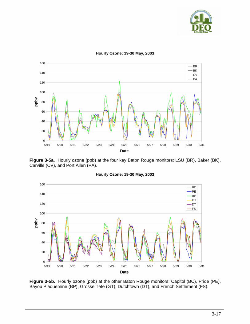
3-17

Hourly Ozone: 19-30 May, 2003

0

20

40

60

80

100

120

140

160

5/19 5/20 5/21 5/22 5/23 5/24 5/25 5/26 5/27 5/28 5/29 5/30 5/31

Date

ppbv

BRBKCVPA

Figure 3-5a. Hourly ozone (ppb) at the four key Baton Rouge monitors: LSU (BR), Baker (BK), Carville (CV), and Port Allen (PA).

Hourly Ozone: 19-30 May, 2003

0

20

40

60

80

100

120

140

160

5/19 5/20 5/21 5/22 5/23 5/24 5/25 5/26 5/27 5/28 5/29 5/30 5/31

Date

ppbv

BCPEBPGTDTFS

Figure 3-5b. Hourly ozone (ppb) at the other Baton Rouge monitors: Capitol (BC), Pride (PE), Bayou Plaquemine (BP), Grosse Tete (GT), Dutchtown (DT), and French Settlement (FS).

3-18

Meteorological conditions in the south-central U.S. during this episode were influenced by the modulation of a relatively weak upper-level low and associated stationary trough over the eastern U.S. This modulation was caused by the passing of several vigorous short waves across the continent. Each exceedance day represented a waning of the strength of the upper-level trough and winds, while multi-day periods between each exceedance day were associated with a strengthening of the upper-level trough. At the surface, this modulation influenced the passing of weak frontal systems from the north during low ozone days, which brought widespread cloud cover and precipitation. These were followed by high pressure, calm/light surface winds, and clear skies on intervening high ozone days. Additionally, temperatures on exceedance days were consistently in the mid-80’s to low 90’s, while non-exceedance days were limited to the high 70’s to mid 80’s. This period was generally characterized by humid conditions, with dewpoint temperatures in the high 60’s to low 70’s. Morning fog was reported at many sites throughout the Gulf States. Hourly average, maximum, and minimum wind speeds and temperature time series among all LDEQ Baton Rouge monitoring sites are displayed in Figure 3-6. A wind rose of the hourly daytime (6 AM to 6 PM) wind speed and direction distribution on exceedance days during this episode is shown in Figure 3-7. Forty-eight hour backward trajectories ending at Baton Rouge at 3 PM on each exceedance day of this episode are shown in Appendix C. Wind speeds indicate a wide range of variation among the monitoring sites, with daytime maximum winds reaching 8-10 mph on some days, while minimum speeds remained within 2-4 mph. On average, winds ranged from 2 to 6 mph, which is consistent with light wind conditions under stagnant high pressure regimes. Temperatures also show a large range of variation among the monitoring sites over the entire diurnal period of each day. This was a rather consistently warm period, except for May 27 during the passage of a cold front. The wind rose indicates mostly westerly to northerly daytime winds with light speeds in the 2-6 mph range during exceedance days. Near calm winds contribute about 23% of the observations. Winds greater than 6 mph were observed just 10% of the time. Back trajectories indicate very stagnant conditions leading up to May 19 (the first exceedance day of the period), with trajectories reaching back to northern Louisiana and east Texas 48 hours prior. Note the curious and rather extreme upward vertical motion (as diagnosed by the EDAS) for parcels ending at 1000 and 2000 m altitude over Baton Rouge. Such upward vertical motion would not be expected during ozone events, so the phenomena driving this motion should be investigated further. On May 24, 28, and 29, back trajectories appear more typical of ozone events in the south-central U.S., with origins several states to the north and anti-cyclonic curvature. Even so, upward motion is diagnosed over the previous 24 hours for two of these later exceedance days. Regional transport into Baton Rouge would be expected during these later three days.

3-19

Hourly Wind Speed: 19-30 May 2003

0

2

4

6

8

10

12

5/19 5/20 5/21 5/22 5/23 5/24 5/25 5/26 5/27 5/28 5/29 5/30 5/31

Date

MPH

MaxAvgMin

Figure 3-6a. Average, maximum, and minimum hourly wind speed (mph) among the Baton Rouge monitors. The extreme winds on May 30 are likely erroneous.

Hourly Temperature: 19-30 May 2003

10

15

20

25

30

35

40

5/19 5/20 5/21 5/22 5/23 5/24 5/25 5/26 5/27 5/28 5/29 5/30 5/31

Date

Deg

ree

C

MaxAvgMin

Figure 3-6b. Average, maximum, and minimum hourly temperature (C) among the Baton Rouge monitors.

3-20

Figure 3-7. Wind rose based on hourly wind speed/direction data from all Baton Rouge monitors between 6 AM and 6 PM on exceedance days.

3-21

3.3.3 September 28-30, 2004 Eight-hour exceedance days during this episode included: September 29 (Wednesday) September 30 (Thursday) Hourly ozone for the period is shown for the four key ozone monitors (Figure 3-8a) and the other monitors (Figure 3-8b). Among the four key monitors, Carville and LSU rise well above the other two on September 28 and 29, while ozone peaks at all sites are quite similar on September 30. A case might be made for a possible THOE on September 29, when Carville and LSU record peaks that are 40 and 60 ppb higher than the other sites, respectively. The Capitol and Dutchtown sites record a similar pattern (Figure 3-8b). The peak timing offsets among these sites suggest the southward transport of an ozone cloud. All other monitors show consistent ozone patterns day-to-day. Meteorological conditions in the south-central U.S. during this episode were characteristic of quiet early fall conditions. Upper air patterns were zonal (west-to-east flow) but generally weak. On September 28, tropical depression “Jeane” was moving north over the Carolinas, having been downgraded from a tropical storm a day earlier. Ozone conditions were primarily driven by surface patterns, which were dominated by a strong high pressure system that extended into the south-central U.S. following a frontal system that passed through on September 28. Surface winds remained calm or light/variable through the period, and skies were clear. Maximum daily temperatures only reached the mid 80’s. Humidity levels were moderate, with dewpoints typically in the low 60s. Hourly average, maximum, and minimum wind speeds and temperature time series among all LDEQ Baton Rouge monitoring sites are displayed in Figure 3-9. A wind rose of the hourly daytime (6 AM to 6 PM) wind speed and direction distribution on exceedance days during this episode is shown in Figure 3-10. Forty-eight hour backward trajectories ending at Baton Rouge at 3 PM on each exceedance day of this episode are shown in Appendix C. This episode is characterized by weak winds at the surface. Wind speeds remained very light on the exceedance days, with maxima only reaching 6-8 mph. A large variation among the monitoring sites is seen by the difference between minimum and maximum speeds. Temperatures were moderate and consistent day-to-day; a wide spread of temperature is also seen among the monitors, especially in the nighttime hours. The wind rose indicates a high frequency of calm to light winds (68% in the 0-4 mph range), mostly from the northwest and secondarily from the east. Winds between 4-6 mph comprise the remaining 23% frequency, with <10% frequency of winds above 6 mph.

3-22

Hourly Ozone: 28-30 September, 2004

0

20

40

60

80

100

120

140

160

9/28 9/29 9/30 10/1

Date

ppbv

BRBKCVPA

Figure 3-8a. Hourly ozone (ppb) at the four key Baton Rouge monitors: LSU (BR), Baker (BK), Carville (CV), and Port Allen (PA).

Hourly Ozone: 28-30 September, 2004

0

20

40

60

80

100

120

140

160

9/28 9/29 9/30 10/1

Date

ppbv

BCPEBPGTDTFS

Figure 3-8b. Hourly ozone (ppb) at the other Baton Rouge monitors: Capitol (BC), Pride (PE), Bayou Plaquemine (BP), Grosse Tete (GT), Dutchtown (DT), and French Settlement (FS).

3-23

Hourly Wind Speed: 28-30 September 2004

0

2

4

6

8

10

12

9/28 9/29 9/30 10/1

Date

MPH

MaxAvgMin

Figure 3-9a. Average, maximum, and minimum hourly wind speed (mph) among the Baton Rouge monitors.

Hourly Temperature: 28-30 September 2004

10

15

20

25

30

35

40

9/28 9/29 9/30 10/1

Date

Deg

ree

C

MaxAvgMin

Figure 3-9b. Average, maximum, and minimum hourly temperature (C) among the Baton Rouge monitors.

3-24

Figure 3-10. Wind rose based on hourly wind speed/direction data from all Baton Rouge monitors between 6 AM and 6 PM on exceedance days.

3-25

The EDAS back trajectories suggest long range transport from the north, extending as far back as Illinois over the 48 hours prior to the first exceedance day (September 29). Trajectories shorten for September 30 as the regional winds calm, but near-surface trajectories continue to reach back into Tennessee. Regional transport into Baton Rouge would be expected during this episode. 3.3.4 April 12-30, 2003

Eight-hour exceedance days during this combined period included: April 13 (Sunday) April 14 (Monday) April 18 (Friday) April 27 (Sunday) April 28 (Monday) April 29 (Tuesday)

Hourly ozone for the period is shown for the four key ozone monitors (Figure 3-11a) and the other monitors (Figure 3-11b). Ozone patterns at all monitors are consistent over much of the period, except for excursions at Baker and Carville on April 18 and 27, respectively. The Carville peak on April 27 may indicate a THOE given that it is ~40 ppb higher than the highest peaks among the other sites. This mid-spring period represents three distinct exceedance episodes separated by extensive cooler, breezier conditions that were associated with weather events. The first three exceedance days are separated from the final three days by more than one week of widespread precipitation. It may be advantageous to model this period as two individual periods. Meteorological conditions in the south-central U.S. during this episode were quite variable, which would be expected of weather during the mid-spring. During the first two exceedance days, upper-air meteorology was dominated by the expansion of a broad, strong ridge that eventually covered the eastern two-thirds of the country following the exit of a vigorous trough eastward over the Atlantic. At the surface, the south-central U.S. was under the influence of strong high pressure, which led to calm or light/variable winds and clear skies. Maximum temperatures only reached the low 80’s. Humidity was rather low, with dewpoints in the 40s to mid-50s. During the intervening days to April 18, a vigorous upper-level short wave induced a surface low pressure system over the central Plains States with some weak frontal systems moving into the south-central U.S. Surface winds along the Gulf Coast increased from the south ahead of the front, and temperatures cooled. However, the period remained dry in Louisiana. On April 18, calm conditions prevailed with the re-establishment of high pressure at the surface and aloft. Maximum temperatures reached the mid-80’s.

3-26

Hourly Ozone: 12-30 April, 2003

0

20

40

60

80

100

120

140

160

4/12

4/13

4/14

4/15

4/16

4/17

4/18

4/19

4/20

4/21

4/22

4/23

4/24

4/25

4/26

4/27

4/28

4/29

4/30 5/1

Date

ppbv

BRBKCVPA

Figure 3-11a. Hourly ozone (ppb) at the four key Baton Rouge monitors: LSU (BR), Baker (BK), Carville (CV), and Port Allen (PA).

Hourly Ozone: 12-30 April, 2003

0

20

40

60

80

100

120

140

160

4/12

4/13

4/14

4/15

4/16

4/17

4/18

4/19

4/20

4/21

4/22

4/23

4/24

4/25

4/26

4/27

4/28

4/29

4/30 5/1

Date

ppbv

BCPEBPGTDTFS

Figure 3-11b. Hourly ozone (ppb) at the other Baton Rouge monitors: Capitol (BC), Pride (PE), Bayou Plaquemine (BP), Grosse Tete (GT), Dutchtown (DT), and French Settlement (FS).

3-27

Subsequent to over one week of poor weather, a broad, low-amplitude ridge was once

again established over the central U.S. on April 26. Over the next few days, this ridge broadened to cover the entire U.S., bringing weak zonal flow aloft. At the surface, strong high pressure built in over the eastern U.S., extending a ridge southward over all the Gulf Coast states. Surface winds remained calm or light/variable through the last three exceedance days, with dry clear skies. Maximum temperatures increased into the low 80’s. Humidity also increased from low dewpoints on April 27 to moderate dewpoints (low 60’s) by the last day.

Hourly average, maximum, and minimum wind speeds and temperature time series among

all LDEQ Baton Rouge monitoring sites are displayed in Figure 3-12. A wind rose of the hourly daytime (6 AM to 6 PM) wind speed and direction distribution on exceedance days during this episode is shown in Figure 3-13. Forty-eight hour backward trajectories ending at Baton Rouge at 3 PM on each exceedance day of this episode are shown in Appendix C. Given the large range of weather patterns over this period, the wind speeds at the Baton Rouge monitors indicate a wide range of variability, and much stronger winds than have been described for previous episodes. However, one can identify the three elevated ozone periods in Figure 3-12a by their suppressed wind speeds. Again, a wide variation of winds is measured by the monitors, even on exceedance days. The cooler, drier mid-spring conditions led to moderate but consistent peak temperatures each day and rather low minimum temperatures for ozone episodes in this area. A consistently large variation in temperature is exhibited among the sites over all hours of the day. The wind rose for exceedance days shows a predominance of calm to light winds up to 4 mph (65%), with a bi-modal direction distribution from the southeast and northwest. The mild speeds of 4-9 mph tended to be southerly through southeasterly. Back trajectories for the first set of exceedance days (April 13-14) show marked anti-cyclonic curvature and downward velocities associated with flow around a strong high pressure area. This is typical of subsidence that can establish strong static stability, stagnation conditions, and shallow boundary layers, all of which are commonly seen during ozone episodes. The trajectories are rather short, indicating weak flow from the north, originating one state away 48 hour prior. On the middle exceedance day (April 18), back trajectories indicate much stronger flow from the northwest, with trajectories originating Oklahoma, Kansas, and Colorado. However, strong subsidence is also present during this time. Over the last three exceedance days (April 27-30), an interesting dynamical situation is shown. Trajectories shift from strong northerly flow, to more moderate easterly flow along the Gulf Coast. All three sets of trajectories indicate anti-cyclonic curvature (suggesting winds around high pressure), but upward velocity is diagnosed, especially for the mid-layer trajectory. Important dynamical influences are present during the entire April 2003 period, although long-range pollutant transport may not be so important during this time as no consistent transport corridors are established for more than a day or two.

3-28

Hourly Wind Speed: 12-30 April 2003

0

2

4

6

8

10

12

14

16

18

20

22

4/12 4/13 4/14 4/15 4/16 4/17 4/18 4/19 4/20 4/21 4/22 4/23 4/24 4/25 4/26 4/27 4/28 4/29 4/30 5/1

Date

MPH

MaxAvgMin

Figure 3-12a. Average, maximum, and minimum hourly wind speed (mph) among the Baton Rouge monitors.

Hourly Temperature: 12-30 April 2003

10

15

20

25

30

35

40

4/12 4/13 4/14 4/15 4/16 4/17 4/18 4/19 4/20 4/21 4/22 4/23 4/24 4/25 4/26 4/27 4/28 4/29 4/30 5/1

Date

Deg

ree

C

MaxAvgMin

Figure 3-12b. Average, maximum, and minimum hourly temperature (C) among the Baton Rouge monitors.

3-29

Figure 3-13. Wind rose based on hourly wind speed/direction data from all Baton Rouge monitors between 6 AM and 6 PM on exceedance days.

3-30

3.3.5 October 4-6, 2003

Eight-hour exceedance days during this episode included: October 4 (Saturday) October 5 (Sunday) Hourly ozone for the period is shown for the four key ozone monitors (Figure 3-14a) and

the other monitors (Figure 3-14b). Peak ozone is quite high over all monitors, with most reaching 100 ppb or more. Among the four key monitors, the LSU and Baker monitors reach the highest levels of nearly 140 ppb, which is 20 ppb above all others. A case might be made for a ROFE at LSU on October 4, but given the high ozone at all monitors, and the high ozone over several afternoon hours at LSU, it would be difficult to attribute this to a single emissions event.

Meteorological conditions during this episode were influenced by the eastward

propagation of a very high-amplitude and deep trough/ridge system over the continent. Most of the energy between these two systems remained well to the north of the Gulf Coast; fairly weak zonal flow was dominant over the southern states. On October 4, a long cold front extended southward from a large low pressure system over the northeast U.S., back into Texas. This slowly propagated southward, and by October 6 was a weak stationary front along the Gulf Coast that brought widespread precipitation to the area. South of this front, a surface high pressure ridge nosed westward from Georgia back into Louisiana, bringing calm to light/variable winds, clear conditions, and maximum temperatures in the mid-80’s on October 4 and 5. With the evolving front/ridge system, humidity varied over these three days, with the lowest values on October 5 (high 50s) and high values on October 6 (high 60s) associated with the increased cloudiness.

Hourly average, maximum, and minimum wind speeds and temperature time series among all LDEQ Baton Rouge monitoring sites are displayed in Figure 3-15. A wind rose of the hourly daytime (6 AM to 6 PM) wind speed and direction distribution on exceedance days during this episode is shown in Figure 3-16. Forty-eight hour backward trajectories ending at Baton Rouge at 3 PM on each exceedance day of this episode are shown in Appendix C. Wind speeds among the Baton rough monitors were exceptionally low during this episode. Peak winds barely reached 5 mph, while the average speed ranged from 1 to 2 mph on the exceedance days. Daily maximum temperatures were consistent day-to-day, but the increasing minimum temperatures reveal the build up of humidity under the stagnant conditions. Not surprisingly, the wind rose exhibits a dominance of calm winds (60%) and the lack of speeds greater than 4 mph (~5%). Directions are skewed toward the east, with fairly even distribution from southeast through northeast. The highest speeds are associated with southeasterly flow. Trajectory plots also demonstrate the high degree of stagnation during this event. On both exceedance days, recirculation patterns cause the back trajectories to remain within the state of Louisiana at all three altitudes. Some subsidence is suggested. This ozone episode would appear to be generated by local emissions only.

3-31

Hourly Ozone: 4-6 October, 2003

0

20

40

60

80

100

120

140

160

10/4 10/5 10/6 10/7

Date

ppbv

BRBKCVPA

Figure 3-14a. Hourly ozone (ppb) at the four key Baton Rouge monitors: LSU (BR), Baker (BK), Carville (CV), and Port Allen (PA).

Hourly Ozone: 4-6 October, 2003

0

20

40

60

80

100

120

140

160

10/4 10/5 10/6 10/7

Date

ppbv

BCPEBPGTDTFS

Figure 3-14b. Hourly ozone (ppb) at the other Baton Rouge monitors: Capitol (BC), Pride (PE), Bayou Plaquemine (BP), Grosse Tete (GT), Dutchtown (DT), and French Settlement (FS).

3-32

Hourly Wind Speed: 4-6 October 2003

0

2

4

6

8

10

12

10/4 10/5 10/6 10/7

Date

MPH

MaxAvgMin

Figure 3-15a. Average, maximum, and minimum hourly wind speed (mph) among the Baton Rouge monitors.

Hourly Temperature: 4-6 October 2003

10

15

20

25

30

35

40

10/4 10/5 10/6 10/7

Date

Deg

ree

C

MaxAvgMin

Figure 3-15b. Average, maximum, and minimum hourly temperature (C) among the Baton Rouge monitors.

3-33

Figure 3-16. Wind rose based on hourly wind speed/direction data from all Baton Rouge monitors between 6 AM and 6 PM on exceedance days.

3-34

3.3.6 May 4-9, 2004

Eight-hour exceedance days during this episode included: May 4 (Tuesday) May 5 (Wednesday) May 6 (Thursday) May 8 (Saturday)

Hourly ozone for the period is shown for the four key ozone monitors (Figure 3-17a) and the other monitors (Figure 3-17b). Daily peak ozone is fairly consistent among the ozone monitors, although Baker is consistently 10-20 ppb higher than the other four key monitors during the middle of the period. Among the other monitors, time shifts in the peaks between southern and northern monitors suggest ozone transport from the north on the first few days, shifting to transport from south to north on the latter days. The data in these figures do not indicate an obvious THOE or ROFE during this period. Meteorological conditions in the south-central U.S. during this episode were dominated by the existence of a very broad, low-amplitude ridge over most of the continent. Conditions in the Gulf States were modulated by a weak trapped low pressure center and trough aloft that started over Mexico and slowly drifted over the south-central U.S. during the period. Flow patterns remained quite weak aloft, changing from zonal early on, to disorganized at the midpoint, to southerly by the end. During the entire period, a surface high pressure system over the southeast U.S. expanded, shifted westward, waned, and finally moved out over the Atlantic by May 9. This caused calm to light/variable winds over the region for most days, with increasing southerly flow off the Gulf during the final day. Skies remained clear on all days except the intervening non-exceedance day of May 7 and the last day, when some light precipitation fell in Louisiana. Interestingly, maximum temperatures started in the high 70’s on May 4 (an exceedance day), and slowly increased to the mid-80’s by May 9. Humidity started low (dewpoints in the mid 50s) and increased through the period to moderate levels (low- to mid-60’s). Hourly average, maximum, and minimum wind speeds and temperature time series among all LDEQ Baton Rouge monitoring sites are displayed in Figure 3-18. A wind rose of the hourly daytime (6 AM to 6 PM) wind speed and direction distribution on exceedance days during this episode is shown in Figure 3-19. Forty-eight hour backward trajectories ending at Baton Rouge at 3 PM on each exceedance day of this episode are shown in Appendix C.

A regular diurnal pattern of winds speed set up over this period, with average daytime ranges from 1 mph in the morning to 5 mph in the afternoon. Like other episode, a wide range of speeds was measured by the network each hour, as indicated by the span between minimum and maximum speeds. However, the overall pattern indicates quiescent conditions. Temperature trended slowly upward during the period from rather mild conditions on the first day, to warm conditions over the last couple days. Like other episodes, a wide range of temperature was seen among the monitors, mostly in the early morning hours.

3-35

Hourly Ozone: 4-9 May, 2004

0

20

40

60

80

100

120

140

160

5/4 5/5 5/6 5/7 5/8 5/9 5/10

Date

ppbv

BRBKCVPA

Figure 3-17a. Hourly ozone (ppb) at the four key Baton Rouge monitors: LSU (BR), Baker (BK), Carville (CV), and Port Allen (PA).

Hourly Ozone: 4-9 May, 2004

0

20

40

60

80

100

120

140

160

5/4 5/5 5/6 5/7 5/8 5/9 5/10

Date

ppbv

BCPEBPGTDTFS

Figure 3-17b. Hourly ozone (ppb) at the other Baton Rouge monitors: Capitol (BC), Pride (PE), Bayou Plaquemine (BP), Grosse Tete (GT), Dutchtown (DT), and French Settlement (FS).

3-36

Hourly Wind Speed: 4-9 May 2004

0

2

4

6

8

10

12

5/4 5/5 5/6 5/7 5/8 5/9 5/10

Date

MPH

MaxAvgMin

Figure 3-18a. Average, maximum, and minimum hourly wind speed (mph) among the Baton Rouge monitors.

Hourly Temperature: 4-9 May 2004

10

15

20

25

30

35

40

5/4 5/5 5/6 5/7 5/8 5/9 5/10

Date

Deg

ree

C

MaxAvgMin

Figure 3-18b. Average, maximum, and minimum hourly temperature (C) among the Baton Rouge monitors.

3-37

Figure 3-19. Wind rose based on hourly wind speed/direction data from all Baton Rouge monitors between 6 AM and 6 PM on exceedance days.

3-38

The wind rose indicates a dominance of calm conditions (>40%), while light winds < 4 mph make up an additional 35% of the distribution. Directions were skewed toward the southwest through southeast quadrants for all speed ranges. Back trajectories for this episode exhibit strong anti-cyclonic curvature and downward motion associated with flow around a strong high pressure system. The daily shift of high pressure from the south-central U.S. to the south-east U.S. and Atlantic is indicated by the eastward shift of trajectories each day. Only on the last day is there evidence of upward motion, as the trajectories show an onshore component from the eastern Gulf with the approach of a weather system to the northwest. Long range ozone transport might have been operative early in the episode, but most near-surface trajectories show on-shore (northward) airflow on later days. If continental pollutants were transported aloft over the Gulf during this time, then there could be a mechanism for transport impacts on later days of the episode if sufficiently deep mixing occurs over Louisiana. 3.3.7 August 11 – September 5, 2000

Eight-hour exceedance days during this episode included: August 11 (Friday) August 13 (Sunday) August 17 (Thursday) August 18 (Friday) August 19 (Saturday) August 20 (Sunday) August 21 (Monday) August 25 (Friday) August 26 (Saturday) August 30 (Wednesday) August 31 (Thursday) September 1 (Friday) September 2 (Saturday) September 3 (Sunday)

Hourly ozone for the period is shown for the four key ozone monitors (Figure 3-20a) and the other monitors (Figure 3-20b). This episode was the last extreme multi-week pollution episode in Baton Rouge. On most days, consistent peak ozone concentrations were measured among all the sites, however some severe short-lived peaks stand out: LSU, Port Allen and Capitol on August 11 (140-160 ppb); Dutchtown on August 18 (130 ppb); LSU, Carville, and Port Allen on August 21 (120-130 ppb); and Baker and Port Allen on August 31 (120-150 ppb). Hourly average, maximum, and minimum wind speeds and temperature time series among all LDEQ Baton Rouge monitoring sites are displayed in Figure 3-21. A wind rose of the hourly daytime (6 AM to 6 PM) wind speed and direction distribution on exceedance days during this episode is shown in Figure 3-22. Forty-eight hour backward trajectories ending at Baton Rouge at 3 PM on each exceedance day of this episode are shown in Appendix C.

3-39

Hourly Ozone: 11 Aug - 5 Sep, 2000

0

20

40

60

80

100

120

140

160

8/11

8/12

8/13

8/14

8/15

8/16

8/17

8/18

8/19

8/20

8/21

8/22

8/23

8/24

8/25

8/26

8/27

8/28

8/29

8/30

8/31 9/1

9/2

9/3

9/4

9/5

9/6

Date

ppbv

BRBKCVPA

Figure 3-20a. Hourly ozone (ppb) at the four key Baton Rouge monitors: LSU (BR), Baker (BK), Carville (CV), and Port Allen (PA).

Hourly Ozone: 11 Aug - 5 Sep, 2000

0

20

40

60

80

100

120

140

160

8/11

8/12

8/13

8/14

8/15

8/16

8/17

8/18

8/19

8/20

8/21

8/22

8/23

8/24

8/25

8/26

8/27

8/28

8/29

8/30

8/31 9/1

9/2

9/3

9/4

9/5

9/6

Date

ppbv

BCPEBPGTDTFS

Figure 3-20b. Hourly ozone (ppb) at the other Baton Rouge monitors: Capitol (BC), Pride (PE), Bayou Plaquemine (BP), Grosse Tete (GT), Dutchtown (DT), and French Settlement (FS).

3-40

Hourly Wind Speed: 11 Aug - 5 Sep 2000

0

2

4

6

8

10

12

8/11

8/12

8/13

8/14

8/15

8/16

8/17

8/18

8/19

8/20

8/21

8/22

8/23

8/24

8/25

8/26

8/27

8/28

8/29

8/30

8/31 9/1

9/2

9/3

9/4

9/5

9/6

Date

MPH

MaxAvgMin

Figure 3-21a. Average, maximum, and minimum hourly wind speed (mph) among the Baton Rouge monitors.

Hourly Temperature: 11 Aug - 5 Sep 2000

10

15

20

25

30

35

40

8/11

8/12

8/13

8/14

8/15

8/16

8/17

8/18

8/19

8/20

8/21

8/22

8/23

8/24

8/25

8/26

8/27

8/28

8/29

8/30

8/31 9/1

9/2

9/3

9/4

9/5

9/6

Date

Deg

ree

C

MaxAvgMin

Figure 3-21b. Average, maximum, and minimum hourly temperature (C) among the Baton Rouge monitors.

3-41

Figure 3-22. Wind rose based on hourly wind speed/direction data from all Baton Rouge monitors between 6 AM and 6 PM on exceedance days.

3-42

Wind speeds were consistently light during the entire period, averaging 1-5 mph, with only occasional afternoon peak winds reaching 10 mph at the maximum site. Minimum afternoon winds rarely exceeded 3 mph among the Baton Rouge sites. Daily temperatures were quite warm over the month as well, and reached up to 40 C (104 F) during the first days of September. As seen for other episodes, there was a wide range of temperatures among the monitoring sites each hour, especially in the early morning. Conditions were also rather humid, as evidenced by the very high daily minimum average temperatures of 25 C (77 F). The wind rose exhibits a fairly consistent speed distribution in the 0 to 6 mph range (covering 90% of total observations), and the frequency of higher speeds is significantly less. The directions are weighted toward the western quadrants, which are associated with the highest speeds, while the northeast direction comprises a secondary maximum. Little wind direction observations were measured from the south through the east. The back trajectories indicate a wide range of transport routes, which would be expected given the large number of exceedance days during this episode. However, anti-cyclonic curvature around high pressure systems is a common trait among most trajectory plots. There are certain days that show marked stagnation, as the trajectories re-circulate within a very short distance over 48 hours, while others indicate the potential of long range transport from the upper Midwest, Ohio Valley, and the southeast U.S. Despite the consistent local wind and temperature conditions measured in Baton Rouge over August and early September 2000, it is clear from these plots that a variety of regional transport conditions exist.

4-1

4.0 MODELING DOMAINS AND DATA AVAILABILITY

This chapter summarizes the model domain definitions for the Baton Rouge 8-hour ozone modeling, including the domain coverage, resolution, map projection, and nesting schemes for the high resolution sub-domains. It also discusses the emissions and aerometric data available from various State and federal agencies for use in model input preparation and performance testing.

4.1 Horizontal Modeling Domain

The 36-km eastern United States (U.S.) horizontal domain for CAMx and EPS will be identical to what is used by the TCEQ in their current 8-hour ozone modeling. This 36-km modeling domain was also selected by the Oklahoma DEQ for their 8-hour ozone EAC SIP modeling after evaluating the effects of the size of the 36-km regional modeling domain on their 8-hour ozone impacts in Tulsa and Oklahoma City (Morris et al., 2005d). Through 2004, both TCEQ and ODEQ were initially using a smaller regional 36-km domain (although much larger than the 36-km domain proposed in the preliminary draft Modeling Protocol for Baton Rouge 8-hour ozone modeling; ICF, 2005). However, when they performed ozone source apportionment modeling on their original 36-km domain they found a larger than expected contribution from the lateral boundary conditions. Thus, the TCEQ and ODEQ expanded the 36-km modeling domain, which not only reduced the influence of the boundary conditions but also allowed them to account for the benefits of the large NOx controls in the Midwest due to the NOx SIP Call on transported ozone into Texas and Oklahoma.

The Baton Rouge CAMx/EPS 12-km modeling domain is defined to include the Gulf

States and most of the Ohio River Valley source region; the new proposed 12-km modeling domain is also larger than the original 36-km domain in the preliminary draft Modeling Protocol. The 4-km modeling domain covers the southern half of Louisiana and the immediate Gulf coastline, and includes the Houston-Galveston and Beaumont-Port Arthur areas in Texas eastward across Mobile Bay to about Pensacola, Florida.

The CAMx air quality and EPS emissions 36/12/4 km modeling domains are aligned

within the MM5 domains. The MM5 modeling domains are offset (larger) from the CAMx/EPS modeling domains by 6 grid cells in each direction. Figure 4-1 displays the nested 36/12/4 km domains proposed to be used in the Baton Rouge 8-hour ozone modeling analysis; the MM5 domains are the outer solid lines, whereas the CAMx/EPS domains are the dotted lines. These grids are based on a Lambert Conformal Projection (LCP) using the same projection as adopted for Texas and Oklahoma. The LCP is defined by the projection parameters listed in Table 4-1.

There is a possibility of boundary noise effects resulting from boundary conditions coming into dynamic balance with MM5’s algorithms. The larger MM5 domain is designed to sequester such errors from the air quality simulation. The buffer region used here exceeds the EPA suggestion of at least 5 grid cell buffer at each boundary. A similar 6 cell buffer is used around the CAMx boundaries for the 12-km and 4-km domains.

4-2

-2592 -2232 -1872 -1512 -1152 -792 -432 -72 288 648 1008 1368 1728 2088 2448-1800

-1440

-1080

-720

-360

0

360

720

1080

1440

1800

Birmingham

Washington

Miami

Tampa

Atlanta

Chicago

Indianapolis

Wichita

Louisville

New Orleans

Shreveport

Boston

Detroit

Minneapolis

Kansas City St. Louis

Charlotte

Omaha

Buffalo

New York

Cincinnati

Cleveland

Columbus

Oklahoma City Tulsa

Philadelphia Pittsburgh

Memphis

Nashville

Austin

Dallas

Houston San Antonio

Virginia Beach

Milwaukee

36 km MM5

36 km

4 km

12 km

Figure 4-1a. Nested 36/12/4 km modeling domains for the Baton Rouge 8-hour ozone modeling study. Dotted line domains are for CAMx/EPS that are nested in the MM5 solid line domains.

4-3

-72 48 168 288 408 528 648 768 888 1008 1128 1248 1368 1488 1608 1728 1848-1332

-1212

-1092

-972

-852

-732

-612

-492

-372

-252

-132

-12

108

228

Birmingham

Jacksonville

Tampa

Atlanta

Indianapolis

Wichita

Louisville

New Orleans

Kansas City St. Louis

Charlotte

Omaha Omaha

Cincinnati

Columbus

Oklahoma City

Tulsa Memphis

Nashville

Dallas

Houston San Antonio

12 km MM5

12 km

4 km

Figure 4-1b. Nested 12/4 km modeling domains for the Baton Rouge 8-hour ozone modeling study. Dotted line domains are for CAMx/EPS that are nested in the MM5 solid line domains.

336 416 496 576 656 736 816 896 976 1056 1136 1216-1200

-1160

-1120

-1080

-1040

-1000

-960

-920

-880

New Orleans

Houston

Figure 4-1c. 4-km Louisiana modeling domain for the Baton Rouge 8-hour ozone modeling study. Red dotted line domain is for CAMx/EPS that are nested in the MM5 domain.

4-4

Table 4-1. Lambert Conformal Projection (LCP) definition for the Baton Rouge 36/12/4 km modeling grid.

Parameter Value Projection Lambert-Conformal 1st True Latitude 30 degrees N 2nd True Latitude 60 degrees N Central Longitude 100 degrees W Central Latitude 40 degrees N

Table 4-2. Grid definitions for MM5, EPS and CAMx.

Table 4-2 lists the number of rows and columns and the definition of the X and Y origin

(i.e., the southwest corner) for the 36/12/4 km domains to be used by MM5, EPS and CAMx. In Table 4-2 “Dot” refers to the grid mesh defined at the vertices of the grid cells while “Cross” refers to the grid mesh defined by the grid cell centers. Thus, the dimension of the dot mesh is equal to the cross mesh plus one. 4.2 Vertical Modeling Domain

The CAMx vertical structure is primarily defined by the vertical grid used in the MM5 modeling. The MM5 model employs a terrain following coordinate system defined by pressure, using multiple layers that extend from the surface to 100 mb (approximately 15 km AGL). A layer averaging scheme is adopted for CAMx simulations to reduce the air quality computational time. The effects of layer averaging were evaluated by WRAP and VISTAS and found to have a relatively minor effect on the model performance metrics when both 34 layer and 19 layer CMAQ model simulations were compared to ambient monitoring data (Morris et al., 2004a). For the Baton Rouge ozone modeling, 16 vertical layers will be used. Table 4-3 lists the mapping from the MM5 vertical layer structure to the CAMx vertical layers. This MM5 structure was taken from the CENRAP configuration and the CAMx structure is also being used in the St. Louis 8-hour ozone modeling.

MODEL COLUMNS DOT(CROSS)

ROWS DOT(CROSS)

XORIGIN (KM)

YORIGIN (KM)

MM5 36 km grid

12 km grid

4 km grid

145 (144)

163 (162)

227 (226)

101 (100)

130 (129)

88 (87)

-2592.0

-72.0

336.0

-1800.0

-1332.0

-1200.0

EPS/CAMx 36 km grid

12 km grid

4 km grid

(69)

(152)

(209)

(67)

(119)

(65)

-108.0

-12.0

356.0

-1584.0

-1272.0

-1156.0

4-5

Table 4-3. Vertical layer definition for MM5 simulations (left most columns), and approach for reducing CAMx layers by collapsing multiple MM5 layers (right columns). Configuration is based upon the CENRAP visibility and St. Louis 8-hour ozone modeling applications.

MM5 CMAQ/CAMx Layer Sigma Pres (mb) Height (m) Depth (m) Layer Pres (mb) Height (m) Depth (m)

34 (top) 0.000 100 18123 2856 16 100 18123 7987 33 0.050 145 15267 2097 32 0.100 190 13170 1659 31 0.150 235 11510 1374 30 0.200 280 10136 1173 15 280 10136 3106 39 0.250 325 8963 1024 28 0.300 370 7938 909 27 0.350 415 7030 817 14 415 7030 2866 26 0.400 460 6213 742 25 0.450 505 5471 680 24 0.500 550 4791 627 23 0.550 595 4163 582 13 595 4163 1635 22 0.600 640 3581 543 21 0.650 685 3038 509 20 0.700 730 2528 386 12 730 2528 664 19 0.740 766 2142 278 18 0.770 793 1864 269 11 793 1864 443 17 0.800 820 1596 174 16 0.820 838 1421 171 10 838 1421 338 15 0.840 856 1251 167 14 0.860 874 1083 164 9 874 1083 324 13 0.880 892 920 161 12 0.900 910 759 79 8 910 759 158 11 0.910 919 680 78 10 0.920 928 601 78 7 928 601 155 9 0.930 937 524 77 8 0.940 946 447 76 6 946 447 152 7 0.950 955 371 75 6 0.960 964 295 75 5 964 295 149 5 0.970 973 220 74 4 0.980 982 146 37 4 982 146 37 3 0.985 987 109 37 3 987 109 37 2 0.990 991 73 36 2 991 73 36 1 0.995 996 36 36 1 996 36 36

0 (ground) 1.000 1000 0 0 0 0 0 0

4-6

4.3 Data Availability

The CAMx modeling systems requires emissions, meteorology, surface characteristics, initial and boundary conditions (IC/BC), and ozone column data for defining the inputs.

4.3.1 Emissions Data

The base year emissions inventory for ozone modeling will be based upon the revised 2002 emissions developed by the CENRAP emission inventory contractor (Strait, Roe and Vukovich, 2004) and by the Texas Commission on Environmental Quality (TCEQ). Emissions for the non-CENRAP states, Mexico and Canada will be based on the latest available inventories that are being used by MRPO, WRAP and VISTAS. These emissions will be augmented by local emissions data for the Baton Rouge 5-Parish area and for Louisiana as available. They will be projected to the base year of the Baton Rouge episodes being modeled. For purposes of air quality model performance evaluation, actual day-specific hourly NOx and SO2 emissions for Electrical Generating Units (EGU) and other large stationary sources that have Continuous Emissions Monitoring (CEM) systems will be used. If appropriate and as data are available, day-specific fire activity data will be also be used in the base case simulations used for model evaluation. For strategy and future year emission runs, “typical year” emissions for these categories will be processed for the base and future years.

As necessary, all emissions will be converted to Area Mobile Source (AMS) and AIRS

Facility System (AFS) format and the data will be processed for air quality modeling using Version 3 of the Emissions Processing System (EPS3). Included in these runs will be the temporal and speciation profiles and cross-reference data provided with EPS3, augmented with any recommended and approved emission profile data obtained from EPA, or prepared by the study team prior to initial emissions modeling. Spatial allocation of the emissions will be based on profiles and allocation factors developed for the modeling grid. Additional description of emissions processing is described in Chapter 5 and emissions QA is described in Appendix A. 4.3.2 Air Quality

Data from ambient monitoring networks for gas species are used in the model performance evaluation. Table 4-4 summarizes ambient gaseous and PM monitoring networks. 4.3.3 Ozone Column Data

Additional data used in the air quality modeling include ozone column data from the

Total Ozone Mapping Spectrometer (TOMS) satellite platform. TOMS data are available for 24-hour average time periods, and are obtained from http://toms.gsfc.nasa.gov/eptoms/ep.html. The TOMS data are used in the CAMx (TUV) radiation models to calculate photolysis rates. Frequently TOMS ozone column data are missing for extended periods so data needs to be filled. The CAMx TUV processor allows for the use of episode average data. If there are large periods of missing TOMS data during a Baton Rouge modeling episode, then we may use monthly or episode average TOMS data and ignore the missing data.

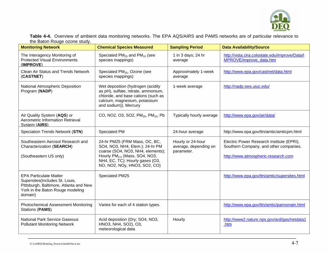
G:\LADEQ\Modeling_Protocol\draft#4\Sec4.doc 4-7

Table 4-4. Overview of ambient data monitoring networks. The EPA AQS/AIRS and PAMS networks are of particular relevance to the Baton Rouge ozone study.

Monitoring Network Chemical Species Measured Sampling Period Data Availability/Source

The Interagency Monitoring of Protected Visual Environments (IMPROVE)

Speciated PM25 and PM10 (see species mappings)

1 in 3 days; 24 hr average

http://vista.cira.colostate.edu/improve/Data/IMPROVE/improve_data.htm

Clean Air Status and Trends Network (CASTNET)

Speciated PM25, Ozone (see species mappings)

Approximately 1-week average

http://www.epa.gov/castnet/data.html

National Atmospheric Deposition Program (NADP)

Wet deposition (hydrogen (acidity as pH), sulfate, nitrate, ammonium, chloride, and base cations (such as calcium, magnesium, potassium and sodium)), Mercury

1-week average http://nadp.sws.uiuc.edu/

Air Quality System (AQS) or Aerometric Information Retrieval System (AIRS)

CO, NO2, O3, SO2, PM25, PM10, Pb Typically hourly average http://www.epa.gov/air/data/

Speciation Trends Network (STN) Speciated PM 24-hour average http://www.epa.gov/ttn/amtic/amticpm.html

Southeastern Aerosol Research and Characterization (SEARCH)

(Southeastern US only)

24-hr PM25 (FRM Mass, OC, BC, SO4, NO3, NH4, Elem.); 24-hr PM coarse (SO4, NO3, NH4, elements); Hourly PM2.5 (Mass, SO4, NO3, NH4, EC, TC); Hourly gases (O3, NO, NO2, NOy, HNO3, SO2, CO)

Hourly or 24-hour average, depending on parameter.

Electric Power Research Institute (EPRI), Southern Company, and other companies.

http://www.atmospheric-research.com

EPA Particulate Matter Supersites(Includes St. Louis, Pittsburgh, Baltimore, Atlanta and New York in the Baton Rouge modeling domain)

Speciated PM25 http://www.epa.gov/ttn/amtic/supersites.html

Photochemical Assessment Monitoring Stations (PAMS)

Varies for each of 4 station types. http://www.epa.gov/ttn/amtic/pamsmain.html

National Park Service Gaseous Pollutant Monitoring Network

Acid deposition (Dry; SO4, NO3, HNO3, NH4, SO2), O3, meteorological data

Hourly http://www2.nature.nps.gov/ard/gas/netdata1.htm

4-8

4.3.4 Meteorological Data

Meteorological data are being generated using the MM5 prognostic meteorological model. Episodic MM5 runs will be performed on the 36/12/4 km domains. Initialization days prior to the Baton Rouge episode will be run on the 36-km grid for 10 days, 12-km grid for 3 days and 4-km grid for 1 day prior to the start of the Baton Rouge ozone episodes. The MM5 model will be started approximately 12 hours prior to the first hour that the data will be used by CAMx/EPS. 4.3.5 Initial and Boundary Conditions Data

For the Baton Rouge ozone simulations we will use a 10-day initialization period on the 36-km grid to eliminate the contribution of initial concentrations. Clean initial conditions (ICs) will be used at the start of the 10-day initialization period. CAMx boundary conditions (BCs) will be based on results from the 2002 CENRAP base case simulation, processed to diurnally-varying monthly averages.

5-1

5.0 MODEL INPUT PREPARATION PROCEDURES

This section describes the procedures to be used in developing the meteorological, emissions, and air quality inputs to the CAMx model for the Baton Rouge 8-hour ozone modeling episodes on the 36/12/4 km grids. The development of the CAMx meteorological and emissions inputs are discussed together with the science options recommended for MM5 and CAMx models. The procedures for developing the initial and boundary conditions and photolysis rates inputs are also discussed along with the model application procedures.

The procedures set forth here are consistent with EPA guidance (e.g., EPA, 1991; 1999;

2005a), other recent 8-hour ozone modeling studies conducted for various State and local agencies using these or other state-of-science modeling tools (see, for example, Tesche et al., 2003a,b,c; Morris et al., 2004a,b; Tesche et al., 2005a), as well as the methods used by EPA in support of the recent Clean Air Interstate Rule (EPA, 2005b) and the Clean Air Mercury Rule (EPA, 2005c). 5.1 Meteorological Inputs 5.1.1 MM5 Model Science Configuration

The MM5 model configuration will be based on recent modeling research and sensitivity testing carried out with the MM5 in Texas (Byun et al., 2005a,b), work at the Iowa Department of Natural Resources (Johnson, 2004), Olerud and co-workers with the VISTAS program (Olerud and Sims, 2004, Abraczinskas et al., 2004), WRAP MM5 modeling (Kemball-Cook et al., 2004) and MM5 modeling to support 8-hour ozone EAC SIP development in Texas, Oklahoma, New Mexico and Colorado (see Table 5-1 for additional details),. 5.1.2 MM5 Input Data Preparation Procedures A brief summary of the MM5 input data preparation procedures we will use are listed below and provided in Table 5-1.

Model Selection: The current version of the non-hydrostatic MM5 (version 3.7) will be used. The MM5 TERRAIN, PREGRID/REGRID, RAWINS/little_r, and INTERPF processors will be used to develop model inputs.

Horizontal Domain Definition: The computational domain on which MM5 will be applied will be sufficiently sized to accommodate the air quality and emissions modeling grids as defined in Figure 4-1 and Tables 4-1 and 4-2. The MM5 36/12/4 km domains are defined with a 6 grid cell buffer in all directions from the air quality modeling domains.

Vertical Domain Definition: The MM5 modeling will employ 34 vertical layers with an approximately 36 meter deep surface layer, based upon the configuration used in the CENRAP modeling. The MM5 vertical domain is presented in both sigma and height coordinates in Table 4-3.

Topographic Inputs: Topographic information for the MM5 will be developed using the NCAR and the U.S. Geological Survey (USGS) terrain databases. The 36-km grid will be

5-2

Table 5-1. MM5 (Version 3.7) model configuration. Science Options Configuration Details

Model Code MM5 version 3.7 (MPP) -- 23 Dec '04 Release Dudhia (1993), Grell et al., (1994) Horizontal Grid Mesh 36/12/4 km 36 km grid 145 x 101 cells Cross Points (add one for dot points) 12 km grid 163 x 130 cells 4 km grid 227 x 88 cells Vertical Grid Mesh 34 Layers; Surface layer ~ 35 m deep Vertically varying; sigma pressure coordinate Domain Depth Surface to ~15 km AGL Top defined by 100 mb Grid Interaction Feedback Two-way nesting with feedback Initialization EDAS Eta Data Assimilation System Boundary Conditions EDAS 40 km resolution Microphysics Mixed Phase Moisture Scheme Reisner II in 36/12/4 km grids Cumulus Scheme Kain-Fritsch 2 subgrid scale cumulus 36/12 km grids only Planetary Boundary Layer ACM Asymmetric Convective Mixing with PX LSM Radiation RRTM Rapid Radiative Transfer Model Vegetation & Land Use USGS 24 Category Scheme 36 km grid 10 min (~18 km) global data Geophysical Data Center 12 km grid 5 min (~9 km) global data Geophysical Data Center 4 km grid High-Resolution (30 sec) NCAR Land Surface Model Pleim-Xiu LSM (ISOIL = 3) Soil moisture from EDAS fields, not PX module Topographic Input 36/12/4 km grid Updated NCAR/PSU data bases Supplied with MM5 Shallow Convection None Sea Surface Temperature EDAS skin temperature Spatially varying 4D Data Assimilation

36 km grid Analysis nudging wind, temp and moisture above PBL, only wind below PBL Wind, temp coeff = 2.5x10-4; mixing ratio coeff = 1x10-5

12 km grid Analysis nudging wind, temp and moisture above PBL, only wind below PBL Wind, temp coeff = 2.5x10-4; mixing ratio coeff = 1x10-5

4 km grid Analysis nudging wind, temp and moisture above PBL, only wind below PBL. Surface wind observation nudging.

Wind, temp coeff = 2.5x10-4; mixing ratio coeff = 1x10-5

Spin-up Spin-up time typically ~12 hrs Spin-up prior to ozone episode simulation

5-3

based the 10 min (~18 km) Geophysical Data Center global data. The 12-km grid will be developed from the 5 min (~9 km) Geophysical Data Center global data, whereas the 4-km terrain heights will be based on 30 second data (~1 km resolution). Terrain data will be interpolated to the model grid using the TERRAIN pre-processor.

Vegetation Type and Land Use Inputs: Vegetation type and land use information will be developed for the 36/12/4 km grids using the most recently released NCAR/PSU databases provided with the MM5 distribution. Standard MM5 surface characteristics corresponding to each land use category will be employed.

Atmospheric Data Inputs: Initialization, boundary conditions and FDDA nudging fields will be based on the 40 km Eta Data Assimilation System (EDAS) fields.

Water Temperature Inputs: The EDAS “skin temperature” field will be used for water temperature inputs.

FDDA Data Assimilation: Standard FDDA data assimilation techniques will be used in this study (see, for example, Byun et al., 2005a; Nielson-Gammon et al., 2005; Olerud and Simms, 2004a,b;and Gao et al., 2000; Kemball-Cook et al., 2005). The MM5 simulations will use the three-dimensional analysis-nudging technique where the predictions are nudged toward a field prepared by regridding the EDAS. For these simulations a nudging coefficient of 2.5x10-4 will be used for winds and temperature and 1x10-5 for mixing ratio on the 36/12/4 km grids. Thermodynamic variables will not be nudged within the boundary layer (i.e., only winds will be nudged within the PBL). In the 4-km grid, surface observation nudging will be performed for winds.

Physics Options: The MM5 model physics to be used in the MM5 simulations will be as follows:

• Kain Fritsch II cumulus parameterization; • ACM PBL that is compatible with the PX LSM; • Plein-Xiu (P-X) Land Surface Model; • Reisner II Mixed Ice Moisture Scheme; and • RRTM Atmospheric Radiation Scheme.

Sensitivity tests will be conducted to evaluate alternative MM5 physics options for one or more

of the Baton Rouge episodes. For example, the Eta PBL and NOAH/OSU LSM schemes will be evaluated as an alternative to the PX/ACM LSM/PBL scheme. 5.1.3 MM5CAMx Reformatting Methodology

The MM5CAMx processor maps MM5 meteorological fields to the format required by CAMx. It also calculates turbulent vertical exchange coefficients (Kz) that define the rate and depth of vertical mixing in CAMx. Steps in the MM5CAMx processing include:

• Reading in meteorological model output files; • Extracting meteorological data for CAMx domain;

5-4

• Collapsing meteorological data if coarser vertical resolution data is requested in CAMx than used in MM5;

• Computing vertical diffusivities (Kz) using three options available to the user;

When feasible it is desirable to use the same layer structure in the air quality model as in the MM5 to prevent errors associated with averaging layer data, and to maintain consistency between data produced by the meteorological model and those used by the chemistry-transport model. However, vertical layer collapsing is typically used to reduce computational costs associated with using large number of vertical layers. Further details on the CAMx modeling domain definitions were provided in Chapter 4 (Table 4-3).

Two sets of vertical turbulent diffusivity options will be invoked in MM5CAMx from the MM5

ACM/P-X runs: (a) the O’Brien scheme (OB70), and (b) the CMAQ scheme. A third option (the TKE method) could also be invoked for the MM5 Eta run. MM5CAMx will be operated initially with a 0.1 m2/s minimum KV (Kz_min) value. 5.1.4 Treatment of Minimum KV The minimum KV value (Kz_min) is an area of ongoing investigation by the CAMx model developers and the scientific user community (e.g., CMAQ developers). EPA initially recommended a 1.0 m2/s Kz_min for CMAQ modeling. However in their ozone forecasting, EPA uses Kz_min values of 0.1 to 2.0 m2/s depending on the amount of urban land use present. To maximize flexibility we will process the MM5 data using MM5CAMx using a 0.1 m2/s Kz_min and then test other Kz_min values (e.g., 1.0 m2/s). The CAMx modeling system contains a utility that produces enhanced minimum Kz (Kz_min) values near the surface to account for increased mixing due to roughness and the urban heat island. The selection of the Kz profiles (O’Brien or CMAQ) and Kz_min approach will be based on the latest thinking, CAMx sensitivity tests and model performance. 5.2 Emission Inputs 5.2.1 Available Emissions Inventory Datasets The emissions inventories developed for the Baton Rouge 8-hour ozone modeling study will be based on the latest 2002 emissions database, as updated by States and the RPOs, augmented by local emission inventories for the Baton Rouge area, local traffic demand model (TDM) output for on-road mobile sources in Baton Rouge, and day-specific emissions for sources with Continuous Emissions Monitoring (CEM) systems (e.g., Electrical Generating Units, EGUs). The year 2002 is the latest emissions year with complete emissions inventories for all states. The base year emissions inventory for the Baton Rouge ozone modeling will be derived from the revised 2002 base case emissions developed by CENRAP emission inventory (EI) contractors (Strait, Roe and Vukovich, 2004). Non-CENRAP state emissions will be based on inventories supplied by the other RPOs (e.g., MRPO and VISTAS) that were developed to be representative of the 2002 year. These emissions will be projected to the base year of the various Baton Rouge ozone episodes (see Chapter 3).

5-5

Local emissions within the 5-Parish Baton Rouge area will be updated with data from local sources as available. Link-based Vehicle Miles Traveled (VMT) data will be used along with the EPA MOBILE6 model to generate on-road mobile source emissions within the Baton Rouge area.

Biogenic emissions will be day-specific and based the MM5 model-derived temperatures using

the GloBEIS biogenic emissions model. MM5 temperature fields will be reviewed and statistically analyzed for the presence of any daytime temperature bias. If a significant bias exists that cannot be removed through any re-configuration of the model, an alternative means of providing gridded temperature fields from observational analyses will be developed.

For model evaluation, day-specific hourly CEM emissions will be used for large stationary

source point sources where available (e.g., EGUs). For the base year projection inventory and future year emission runs, “typical year” emissions for these large stationary sources will be processed.

These emissions will be converted to the Area Mobile Sources (AMS) and AIRS Facility System (AFS) formats used by the EPS emissions model. 5.2.2 Development of CAMx-Ready Episodic Emissions Inventories

CAMx-ready emissions will be generated by the EPS3 suite of programs. Table 5-2 summarizes the EPS3 configuration to be used.

Emissions inventory development for episodic 8-hour ozone modeling must address several

source categories including: (a) stationary point sources, (b) area sources, (c) on-road mobile sources, (d) non-road mobile sources, and (e) biogenic sources. For this analysis, these estimates must be developed to support the episodes being modeled (see Chapter 3).

Development of an emissions inventory customized for the Baton Rouge 5-Parish area requires a merging of: (a) the most recent pertinent regional inventory and (b) available high-resolution, locale-specific emissions estimated by local, state, and regional agencies in the region. Local air regulatory and transportation planning agencies are generally the best sources of domain-specific activity and control factors to use in developing the base year emissions. Often, these local emissions data sets come from a variety of sources, frequently in different formats. Contacts with CENRAP’s emission inventory contractors, other RPOs, and the U.S. EPA will be established and formal requests made for inventory corrections, updates and ancillary data pertinent to the modeling of emissions in their jurisdictions. Where feasible these updated emissions data sets will be acquired and will be used to create day-specific modeling inventories for the Baton Rouge area for each of the ozone episodes to be modeled.

CAMx requires two emission input files: (1) low level gridded emissions that are emitted

directly into the first layer of the model from sources at the surface with little or no plume rise; and (2) elevated point sources (stacks) with plume rise calculated from stack parameters and meteorological conditions. Hour emissions are required for NO, NO2, CO, several classes of VOCs and other pollutants as available. The VOC classes used will depend upon the chemical mechanism selected. Although the CB4 chemical mechanism has been used in most recent 8-hour ozone EAC SIPs and by the RPOs for their regional modeling, indications from the HGB modeling suggest that the effects of HRVOC emissions on ozone formation may be better simulated using the SPARC chemical

5-6

Table 5-2. EPS (Version 3) configuration. Emissions Component Configuration Details

Model Code EPS Version 3 Horizontal Grid Mesh 36/12/4 km 36 km grid 69 x 67 cells 12 km grid 152 x 119 cells 4 km grid 209 x 65 Area Source Emissions CENRAP/VISTAS/MRPO/LDEQ

On-Road Mobile Sources CENRAP/VISTAS/MRPO/LDEQ Baton Rouge TDM, MOBILE6

Point Sources CENRAP/VISTAS/MRPO/LDEQ CEM day-specific for EGUs

Off-Road Mobile Sources CENRAP/VISTAS/MRPO/LDEQ EPA NONROAD model

Emissions Data Sources 2002 Base B CENRAP States 2002 Base K MRPO States 2002 Base G VISTAS States 2002 TDM VMT for BTR 2002-2005 LDEQ Data Biogenic Sources GloBEIS Temporal Adjustments Seasonal, day, hour Based on latest collected information

Chemical Speciation Revised CB4 Chemical Speciation SAPRC Speciation (optional) EPA study

Gridding Spatial Surrogates based on landuse Growth and Controls TBD Quality Assurance QA Tools in EPS; PAVE plots

5-7

mechanism. Given that HRVOC emissions may also be important for many of the Baton Rouge ozone exceedance days, use of the SAPRC chemical mechanism will be considered. 5.2.2.1 Episodic On-Road Mobile Source Emissions

The inputs needed to perform on-road mobile sources modeling for the Baton Rouge episodes on the 36/12/4 km grids include the county-level vehicle miles traveled (VMT) for the entire modeling domain (36-km grid) and the link-based VMT for the urbanized portion of the Baton Rouge area. In addition to the link-based VMT data, GIS-based data specifying the locations of the links from transportation modeling will be required. Vehicle class-specific speciation and temporal profiles will be taken from EPS3 default files, unless additional information can be accessed for this study.

As noted previously, much of the data necessary for this task are currently available from the

Regional Planning Organizations (RPOs). County-level VMT and MOBILE6 input files are available for the CENRAP, WRAP, VISTAS and Midwest RPO (MRPO). The starting point for the on-road mobile source emissions modeling would be the most current CENRAP mobile source emissions inventory. The VMT data for the regional grids (36 and 12 km) would be projected to the base year(s) of the Baton Rouge episodes.

For the finer scale 4-km grid, link-based VMT data from a TDM will be used along with the

EPA MOBILE6 model and MM5 temperatures to generate gridded day-specific on-road mobile source emissions. Again, if a significant temperature bias exists that cannot be removed through any re-configuration of MM5, an alternative means of providing gridded temperature fields from observational analyses will be developed. Whereas the on-network emissions estimates are spatially allocated based on link location and subsequently summed to the grid cell level, the off-network emissions estimates are spatially allocated based on a combination of the FHWA version 2.0 highway networks and population. For the Baton Rouge 36/12 km modeling, no link-based data will be used.

The EPA MOBILE6, interfaced with EPS3, will be used to develop the base year on-road

mobile source emissions estimates for CO, NOx, PM, and VOC emissions. The MOBILE6 parameters, vehicle fleet descriptions, and VMT estimates will be combined with gridded, episode-specific temperature data to calculate the gridded, temporal emission estimates. The MOBILE6 emissions factors are based on episode-specific temperatures predicted by the meteorological model. Further, the MOBILE6 emissions factors model accounts for the following:

• Weekly average minimum/maximum temperatures; • Facility speeds; • Locale-specific inspection/maintenance (I/M) control programs, if any; • Adjustments for running losses; • Splitting of evaporative and exhaust emissions into separate source categories; • VMT, fleet turnover, and changes in fuel composition and Reid vapor pressure (RVP).

The primary input to MOBILE6 is the MOBILE shell file. The MOBILE shell contains the

various options (e.g. type of inspection and maintenance program in effect, type of oxygenated fuel program in effect, alternative vehicle mix profiles, RVP of in-use fuel, operating mode) that direct the calculation of the MOBILE6 emissions factors.

5-8

5.2.2.2 Episodic Biogenic Source Emissions

Biogenic emissions will be generated using the GloBEIS biogenic emissions model. GloBEIS uses high resolution GIS data on plant types and biomass loadings, MM5 or objectively-analyzed surface temperature fields, and solar radiation (modeled or satellite-derived) to develop hourly emissions for biogenic species on the 36/12/4 km grids. GloBEIS generates gridded, speciated, temporally allocated emission files. 5.2.2.3 Point Source Emissions

Point source emissions will be taken from the 2002 RPO database updated with any local information for the Baton Rouge area. These emissions will be projected to the base year of the Baton Rouge episode as needed. The locations of the point sources will be converted to the LCP coordinate system used in the modeling. They will be processed by EPS to generate the temporally varying (i.e., day-of-week and hour-of-day) speciated emissions needed by CAMx, using standard EPS default profiles by source category.

For large point sources with CEM data, the hourly CEM data for the episode periods will be

processed and used as input for the current year actual base case simulations. However, for the ozone projections we will use the average current year emissions from these sources. 5.2.2.4 Area and Non-Road Source Emissions

County level area source emissions will be taken from the RPO 2002 emissions inventory augmented with any local data and projected tom the Baton Rouge episode years(s). The area sources will be spatial allocated to the grid using an appropriate surrogate distribution (e.g., population for home heating, etc.). The area sources will be temporally allocated by month and by hour of day using the EPS default source-specific temporal allocation factors. Non-road mobile source emissions will be calculated using EPA’s NONROAD model to generate county-level emissions. Local data regarding equipment usage will be used to update the data in the NONROAD model as available. The non-road mobile source emissions will be spatially allocated to the grid using an appropriate surrogate distribution (airport locations for aircraft and airport related emissions, railways for locomotive emissions, agricultural land use category for agricultural equipment, etc.). The EPS source-specific temporal and speciation allocation profiles will be used. 5.2.2.5 Wildfires, Prescribed Burns, Agricultural Burns

If there are indications of any fires present near the Baton Rouge area, or within the south-central U.S., during any of the episodes they will be accounted for in the model as information is available. 5.2.2.6 QA/QC and Emissions Merging

The emissions will be processed by major source category in several different “streams”, including area sources, on-road mobile sources, non-road mobile sources, biogenic sources, non-CEM point sources, CEM sources using day-specific hourly emissions, CEM sources using average emissions and, as available, emissions from fires. Separate Quality Assurance (QA) and Quality Control (QC) will be performed for each stream of emissions processing and in each step. EPS3

5-9

includes advanced quality assurance features that includes error logs when emissions are dropped or added. In addition, we will generate visual displays that include:

• Spatial plots of the hourly emissions for each major species (e.g., NOx, VOC, some

speciated VOC and CO); • Vertical average emissions plots for major species and each of the grids; • Diurnal plots of total emissions by major species; and • Summary tables of emissions for major species for each grid and by major source category.

This QA information will be examined against the original point and area source data and

summarized in an overall QA/QC assessment. Scripts to perform the emissions merging of the appropriate biogenic, on-road, non-road, area,

low-level, fire, and point emission files will be written to generate the CAMx-ready two-dimensional day-specific hourly speciated gridded emission inputs. The point source and, as available elevated fire, emissions would be processed into the day-specific hourly speciated emissions in the CAMx-ready point source format.

The resultant CAMx model-ready emissions will be subjected to a final QA using spatial maps,

vertical plots and diurnal plots to assure that: (1) the emissions were merged properly; (2) CAMx inputs contain the same total emissions; and (3) to provide additional QA/QC information.

5.2.3 Use of the Plume-in-Grid (PiG) Subgrid-Scale Plume Treatment

The Plume-in-Grid (PiG) sub-model treats the early plume chemistry and dynamics of

emissions from point sources and then releases the emissions into the grid model farther downwind at such time that the plume is adequately resolved by the grid. There are currently two PiG options in the CAMx model:

• GREASD PiG: treats the early plume dynamics and inorganic NOx chemistry, and releases the emissions from the PiG to the grid model when organic chemistry starts being important; and

• IRON PiG: treats the full CB4 or SAPRC chemistry at all downwind distances.

The GREASD PiG was designed for large NOx point source plumes, where the early evolution of the plume is dominated by NOx and inorganic chemistry. Because of the high NOx in these plumes, the mass they carry are typically released to the grid model at the time that organic chemistry becomes important.

The IRON PiG uses full chemistry and is appropriate for both NOx and VOC plumes. If the PiG is to be used for HRVOC emissions, then the IRON PiG would be the appropriate choice. Currently the CAMx model can only use one PiG module in each run (i.e., it cannot run point source X with GREASD PiG and point source Y with IRON PiG in the same run).

Large NOx plumes, and potentially HRVOC sources as characterized in the inventory, will be selected for treatment by the subgrid-scale PiG module. The selection of which sources to be treated by the PiG module will be made after a review of the inventory. Tests will likely be conducted to

5-10

determine the sensitivity of the ozone estimates in the Baton Rouge area to the use of the different PiG modules, as well as use of ultra-high resolution (~1 km) flexi-nests applied over the locations of HRVOC sources.

5.2.4 Products of the Emissions Inventory Development Process

In addition to the CAMx-ready input files generated for each hour of all days modeled in the Baton Rouge episodes, a number of quality assurance (QA) files will be prepared and used to check for gross errors in the emissions inputs. Importing the model-ready emissions into PAVE and looking at both the spatial and temporal distribution of the emission provides insight into the quality and accuracy of the emissions inputs.

• Visualizing the model-ready emissions with the scale of the plots set to a very low value, we can determine whether there are areas omitted from the raw inventory or if emissions sources are erroneously located in water cells;

• Spot-checking the holiday emissions files to confirm that they are temporally allocated like Sundays;

• Producing pie charts emission summaries that highlight the contribution of each emissions source component (e.g. nonroad mobile);

• Normalizing the emissions by population for each state will illustrate where the inventories may be deficient and provide a reality check of the inventories.

State inventory summaries prepared prior to the emissions processing will be used to compare against EPS output report totals generated after each major step of the emissions generation process. To check the chemical speciation of the emissions to CB-IV and/or SAPRC species, we will compare reports generated with EPS to target these specific areas of the processing. For speciation, the inventory state import totals will be compared against the same state totals with the speciation matrix applied. These reports will be generated for a representative weekday in each of the episodes for each of these selected states. The quantitative QA analyses often reveal significant deficiencies in the input data or the model setup. It may become necessary to tailor these procedures to track down the source of each major problem. As such, one can only outline the basic quantitative QA steps that we will perform in an attempt to reveal the underlying problems with the inventories or processing. Following are some of the reports that may be generated to review the processed emissions:

• State and county inventory totals for each source category. • State and county totals after spatial allocation for each source category. • State and county totals by day after temporal allocation for each source category for

representative days. • State and county totals by model species after chemical speciation for each source category. • State and county model-ready totals (after spatial allocation, temporal allocation, and

chemical speciation) for each source category and for all source categories combined. • If elevated source selection is chosen by user, the report indicating which sources have been

selected as elevated and plume-in-grid will be included. • Totals by source category code (SCC) from the inventory for area, mobile, and point

sources.

5-11

• Totals by state and SCC from the inventory for area, mobile, and point sources. • Totals by county and SCC from the inventory for area, mobile, and point sources. • Totals by SCC and spatial surrogates code for area and mobile sources. • Totals by speciation profile code for area, mobile, and point sources. • Totals by speciation profile code and SCC for area, mobile, and point sources. • Totals by monthly temporal profile code for area, mobile, and point sources. • Totals by monthly temporal profile code and SCC for area, mobile, and point sources. • Totals by weekly temporal profile code for area, mobile, and point sources. • Totals by weekly temporal profile code and SCC for area, mobile, and point sources. • Totals by diurnal temporal profile code for area, mobile, and point sources. • Totals by diurnal temporal profile code and SCC for area, mobile, and point sources. • PAVE plots of gridded inventory pollutants for all pollutants for area, mobile, and point

sources. 5.2.5 Future-Year Emissions Modeling Future-year emission inputs will be generated by EPS by projecting the current year (e.g., 2002) inventory using growth and control factors. Because of the unusual nature of growth in Baton Rouge due to Hurricane Katrina (doubled population in a year), standard growth assumptions may not be applicable. This is an area that will be studied in more detail as the Baton Rouge 8-hour ozone study progresses. 5.3 Photochemical Modeling Inputs 5.3.1 CAMx Science Configuration and Input Configuration

This section describes the model configuration and science options to be used in the Baton Rouge 8-hour ozone modeling effort. Table 5-3 summarizes the CAMx configuration to be used. The latest version of CAMx (either v4.31 or v4.40) will be used in the Baton Rouge modeling.

As indicated in the CAMx model setup defined in Table 5-3, three grids will be employed in

which 12- and 4-km nests will be introduced into the simulation over the 10-day spinup period prior to the first day of each episode (see below). All grids will be run together in 2-way interactive mode (as opposed to 1-way mode as employed in CMAQ). The PPM advection solver will be used along with the spatially varying (Smagorinsky) horizontal diffusion approach. K-theory will be used for vertical diffusion.

Initially, the CB-IV gas-phase chemical mechanism is selected because it has been widely used

by most recent 8-hour ozone EAC SIPs as well as by the RPOs (e.g., CENRAP, MRPO, VISTAS, etc.). However, recent modeling in the Houston Galveston Brazoria (HGB) area has indicated that a better representation of the effects of HRVOC emissions may be obtained using the SAPRC99 chemical mechanism. Thus, the modeling team will also evaluate the suitability and advantages of modeling using the SAPRC chemistry.

5-12

Meteorological Inputs: The MM5-derived meteorological fields will be prepared CAMx using MM5CAMx. Several alternative vertical diffusivity options will be generated for CAMx input and evaluated in sensitivity tests, as described earlier.

Initial/Boundary Conditions: The initial and boundary conditions will be derived from the CENRAP RPO regional modeling for the calendar year 2002 on the RPO continental US 36-km grid. For Baton Rouge episodes from 2002, the CAMx initial concentrations (ICs) and boundary conditions (BCs) would be day-specific and hourly from the CENRAP 2002 Base Case CAMx simulation. For Baton Rouge episodes outside of the 2002 year, monthly average diurnal profiles would be constructed.

Photolysis Rates: The modeling team will prepare the photolysis inputs as well as albedo/haze/ozone/snow inputs for CAMx based on Total Ozone Mapping Spectrometer (TOMS) data. For CAMx the TUV processor will be used. If there are periods of more than a couple of days where daily TOMS data are unavailable, monthly average TOMS data will be used.

Landuse: The team will generate landuse fields based on USGS GIRAS data using tools provided by the LDEQ contractors. Spin-Up Initialization: RPO modeling for large 36-km domains, like that proposed for the Baton Rouge modeling, has shown that 10-15 days of spin up is needed to eliminate the influences of initial concentrations. For the Baton Rouge episodes we also proposed to use 10 days of spin up for the 36-km domain, invoking the higher resolution grids near the start of the ozone episodes as follows:

• 36 km grid: 10 days of initialization; • 36/12 km grid: 3 days of initialization; • 36/12/4 km grid: 1 day of initialization.

5-13

Table 5-3. CAMx (Version 4.3 or 4.4) model configuration. Science Options Configuration Details

Model Code CAMx (v4.31) – April 2006 Release see: www.camx.com; potentially v4.40 Horizontal Grid Mesh 36/12/4 km 36 km grid 69 x 67 cells 12 km grid 152 x 119 cells 4 km grid 209 x 65 Vertical Grid Mesh 16 vertical layers, defined by MM5 Layer 1 thickness ~ 35 m Grid Interaction Two-way nesting Initial Conditions Default – 10 day spin-up on 36 km grid Clean EPA default conditions

Boundary Conditions Hourly day-specific for 2002 episodes; monthly average diurnally varying for other years

Based on CENRAP 2002 Base Case simulation

Emissions Baseline Emissions Processing EPS3

Sub-grid-scale Plumes Plume-in-Grid for major NOx sources and potentially HRVOC sources

GREASD-PiG NOx chemistry plume model, IRON-PiG full chemistry plume model

Chemistry

Gas Phase Chemistry CBM-IV with isoprene and NOx updates SAPRC chemistry as option Gery et al., (1989). Includes re-nitrification reactions

Meteorological Processor MM5CAMx Compatible with CAMx v4.3 Horizontal Diffusion Spatially varying K-theory with Kh grid size dependence Vertical Diffusion Kv (O'Brien '70, CMAQ, TKE methods) Sensitivity tests to Kz methods

Diffusivity Lower Limit Kz-min = 0.1 to 1.0 m2/s Run MM5CAMx with Kz_min = 0.1 m2/s; sensitivity tests for Kz_min

Deposition Schemes Dry Deposition Wesley resistance scheme Wesley (1989) Wet Deposition CAMx-specific formulation rain/snow/graupel Numerics Gas Phase Chemistry Solver Chemical Mechanism Compiler-- Fast Solver ENVIRON (2004) Vertical Advection Scheme Fully implicit scheme Horizontal Advection Scheme Piecewise Parabolic Method (PPM) scheme

Integration Time Step Wind speed dependent ~0.5-1 min (4-km), 1-5 min (12-km), 5-15 min (36-km)

6-1

6.0 OZONE MODEL PERFORMANCE EVALUATION This chapter describes the model performance evaluation from which to establish reliable CAMx 8-hour ozone modeling for the Baton Rouge 5-Parish area. In general terms, this process consists of the following cycle:

• Exercise the modeling system for the base case, attempting to replicate the time and space behavior of the observed 1-hour and 8-hour ozone concentration fields as well as concentrations of precursor and product species;

• Evaluate the model’s fidelity in simulating ozone and precursor/product species using a two-step process consisting of: (a) an initial “screening model performance evaluation” (SMPE) process, and if the modeling results pass the screening analysis, (b) a “refined model performance evaluation” (RMPE) consisting of progressively more stressful testing procedures involving multi-species, multi-scale surface and aloft model performance evaluation (MPE);

• Identify sources of error and/or compensating biases, through evaluation of preprocessor models (MM5, EPS), air quality model inputs, concentrations aloft, mass budgets and conservation, process analysis, etc;

• Through a documented process of diagnostic and sensitivity investigation, pinpoint and correct the performance problems via model refinement, additional data collection and/or analysis, or theoretical considerations;

• Re-run the model for the base case and re-evaluate performance until adequate, justifiable performance is achieved, or time and/or resources are expended, or the episode is declared unsuited for further use based on documented performance problems.

To an extent, some or all of these steps will be taken by the LDEQ modeling team for each of the Baton Rouge ozone episodes, ideally culminating in a suite of episodes demonstrated to exhibit sufficiently minimal bias and error that they may be used reliably to evaluate 8-hour ozone control strategies and to perform an 8-hour ozone attainment demonstration. In the following subsection, we briefly identify the steps that will be taken by the LDEQ modeling team in constructing and evaluating the CAMx base cases for 8-hour ozone SIP development in Baton Rouge. 6.1 Establishing Base Case CAMx Simulations for Baton Rouge Episodes 6.1.1 Setting Up and Exercising CAMx Base Cases The LDEQ modeling team will select the final model configurations for the CAMx base case simulations for each episode (see Chapter 5). The modeling team will define the recommended final model configurations based on results from the initial configuration (see Tables 5-1 through 5-4) and the following factors:

• Model performance obtained using the initial model configurations and input data; • Model performance for base case sensitivity tests; • The modeling team’s knowledge of the CAMx model configurations and associated

attributes;

6-2

• Experience performing sensitivity tests and model performance evaluation for CENRAP, VISTAS, MRPO, WRAP and numerous other studies including ozone SIP and EAC studies; and

• Comments from EPA and other participants. The objective in identifying optimum model configurations is to obtain the best performance for the right reasons consistent with sound science and EPA guidance. Sometimes, decisions must be made that trade off better/poorer model performance for one pollutant against another, or for one episode against another. These factors will be considered and potential issues discussed among the LDEQ modeling team, EPA and others. Based on the analysis and comments from EPA and other interested parties, the LDEQ modeling team will select the final ozone model configurations. 6.1.2 Use of Sensitivity, Source Apportionment, and Related Diagnostic Probing Tools

The Baton Rouge ozone study may utilize several diagnostic and probing tools to further test and understand the CAMx base case ozone simulations. The use of these tools is discussed below.

Traditional Sensitivity Testing: Traditional sensitivity testing may be performed using the CAMx model. Once each model is operating properly for each base case, sensitivity runs may be performed to explore response to emissions changes as well as changes in key input parameters. These sensitivity runs serve two purposes: • Aid in helping to define appropriate emissions control scenarios; and • Provide episode-specific model uncertainty information that may be used later in

“Weight of Evidence” analyses in support of the 8-hour ozone attainment demonstration. Ozone Source Apportionment: Focused use of ozone source apportionment technology (OSAT) for selected episodes may be employed to better understand model response and to aid in the design of control strategies. The value of source apportionment modeling for subsequent stages of the Baton Rouge modeling study is that these calculations will help to: • Assess the contribution of sources in the Louisiana region and surrounding states to

ozone concentrations at key Baton Rouge receptor locations; and • Identify the particular source categories that may contribute the most to elevated 8-hour

ozone concentrations at various nonattainment monitors. DDM Sensitivity Modeling: Another type of sensitivity that may be performed entails the use of the Direct Decoupled Method (DDM) technology in CAMx. For one or more episodes, DDM may be set up and exercised to produce a numerically intensive, direct sensitivity/uncertainty analysis. DDM can provide information on the sensitivity of ozone to model inputs (e.g., IC, BC, specific emissions). For example, it was used in the HGB area to identify where locations of potential HRVOC emissions would be that could explain the rapid rise in ozone at a particular time and location (i.e., assuming that VOC emissions are missing from the inventory, what emissions locations would best explain observed high ozone levels?).

6-3

Process Analysis: Process Analysis is a tool in CAMx to extract additional information about the various physical and chemical processes in the model that produced the ozone concentrations. Information on VOC-limited versus NOx-limited ozone formation, importance of local production versus entrainment of ozone aloft and identification of the contributions of individual VOC species to ozone formation (e.g., HRVOCs) are the types of information that can be obtained with Process Analysis. It can be a powerful tool for diagnosing the causes of poor model performance.

6.2 Evaluation of CAMx Base Cases for the Baton Rouge Episodes

This section describes the procedures for evaluating the performance of the meteorological and photochemical models using the available aerometric data sets for the Baton Rouge ozone episodes. 6.2.1 Overview

Model performance evaluation (MPE) is the process of testing a model’s ability to accurately estimate observed atmospheric properties over a range of synoptic and geophysical conditions. When conducted thoughtfully and thoroughly, the process focuses and directs the continuing cycle of model development, data collection, model testing, diagnostic analysis, refinement, and re-testing. Below we summarize the philosophy and objectives that will govern the evaluation of the MM5 and CAMx models for the Baton Rouge 8-hour ozone application. Specific evaluation methods are identified that will be employed to judge the suitability of the meteorological and air quality models for regulatory applications, using common statistical measures and graphical procedures to elucidate model performance. This evaluation plan conforms to the procedures recommended by the EPA (1991; 1999; 2005a) for 1-hour and 8-hour ozone attainment demonstration modeling.

We begin by establishing a framework for assessing whether the EPS/MM5/CAMx

modeling system (i.e., the emissions, meteorological and dispersion models and their supporting data sets) perform with sufficient reliability to justify their use in developing 8-hour ozone control strategies for the Baton Rouge nonattainment area. The models’ reliability will be assessed given consideration to the following principals:

The Model Should be Viewed as a System: When we refer to evaluating a "model", we mean this in the broad sense. This includes not only the CAMx photochemical model, but its various components: companion preprocessor models (i.e., the EPS emissions and the MM5 meteorological models), the supporting aerometric and emissions data base, and any other related analytical and numerical procedures used to produce modeling results. A principal emphasis in the model testing process is to identify and correct flawed model components;

Model Acceptance is a Continuing Process of Non-Rejection: Over-reliance on explicit or implied model "acceptance" criteria should be avoided for the reasons identified by Roth et al. (2005). This includes EPA’s ozone performance goals (EPA, 1991). Models should be accepted gradually as a consequence of successive non-rejections. Over time, confidence in a model builds as it is exercised in a number of different applications (hopefully involving

6-4

stressful performance testing) without encountering major or fatal flaws that cause the model to be rejected;

Criteria for Judging Model Performance Must Remain Flexible: The criteria for judging the acceptability of model performance should remain flexible, recognizing the challenging requirement of the Baton Rouge region; and

Previous Experience Used as a Guide: Previous photochemical modeling experience serves as a primary guide for judging model acceptability. Interpretation of the CAMx modeling results for each episode, against the backdrop of previous modeling experience, will aid in identifying potential performance problems and suggest whether the model should be tested further or rejected.

A rigorous ozone model evaluation in typical regulatory applications consists of two

components. The operational evaluation entails an assessment of the model’s ability to correctly estimate surface meteorological or air quality variables largely independent of whether the actual process descriptions in the model are accurate. The operational evaluation essentially tests whether the predicted surface meteorological and air quality fields are reasonable, consistent and agree adequately with routinely available observations. In this study, the operational evaluations focus on the various model’s reliability in reproducing hourly-average surface wind speed, wind direction, temperature, mixing ratio and ozone concentrations across the 4-km Louisiana domain with particular emphasis on the Baton Rouge area.

The scientific evaluation addresses the realism of the meteorological and air quality processes simulated by the models through testing the model as an entire system (i.e., not merely focusing on surface wind, temperature or ozone predictions) as well as its component parts. The scientific evaluation seeks to determine whether the model’s behavior, in the aggregate and in its component modules, is consistent with prevailing theory, knowledge of physical processes, and observations. The main objective is to reveal the presence of bias and internal (compensating) errors in the model that, unless discovered and rectified or at least quantified, may lead to erroneous or fundamentally incorrect decisions based on model usage. Ideally, the scientific evaluation consists of a series of diagnostic and mechanistic tests aimed at: (a) examining the existence of compensatory errors, (b) determining the causes of failure of a flawed model, (c) stressing a model to ensure failure if indeed the model is flawed, and (d) providing additional insight into model performance beyond that supplied through routine, operational evaluation procedures.

Practically, a rigorous scientific evaluation is seldom feasible due to the absence of the specific measurements needed to test the process modules (e.g., soil moisture, Reynold’s stress measurements, PBL heights, trace gas species, and so on). Accordingly, the overall model performance evaluation in this study is constrained mainly to operational testing of the MM5 models’ primary meteorological outputs (i.e., wind speed, wind direction, temperature, and moisture) and the CAMx model’s predictions of ozone, NOx, CO and potentially VOC. However, some components of the scientific evaluation of the air quality model are possible through examination of ground-level and aloft primary and product species and species ratios. In addition, corroborative analyses involving joint analysis of emissions inventory estimates, air quality model predictions and ambient measurements adds to the scientific evaluation.

6-5

6.2.2 Meteorological Model Evaluation Methodology

Meteorological inputs required by the CAMx model include hourly estimates of the three-dimensional distribution of winds, temperatures, mixing ratio, pressure, clouds, and precipitation, and other physical parameters or diagnosed quantities such as turbulent mixing rates (i.e., eddy diffusivities) and planetary boundary layer heights. Accordingly, the objective of the MM5 performance evaluation is to assess the adequacy of the surface and aloft meteorological fields for the Baton Rouge ozone modeling episodes.

6.2.2.1 Components of the Baton Rouge MM5 Evaluation The MM5 modeling system is well-established with a rich development and refinement history spanning more than two decades (Seaman, 2000). The model has seen extensive use worldwide by many agencies, consultants, university scientists and research groups. Thus, the current version of the model, as well as its predecessor versions, has been extensively "peer-reviewed" and considerable algorithm development and module testing has been carried out with all of the important process components. Given that the MM5 model code and algorithms have already undergone significant peer review, performance testing of the MM5 model in this study will be focused on an operational evaluation.

Typically, the scope of the scientific evaluation is limited by the availability of special

meteorological observations (radar profiler winds, turbulence measurements, PBL heights, precipitation and radiation measurements, inert tracer diffusion experiments, and so on). Unfortunately, since these types of measurements may be limited over Baton Rouge during the modeling episodes, a meaningful scientific evaluation of the MM5 may not be possible in this study. However, if the operational evaluation presented in subsequent chapters is performed thoroughly, they are expected to be sufficient to serve as the basis for judging whether the model is operating with sufficient reliability over the Baton Rouge domain to be used in the photochemical modeling portion of this study. 6.2.2.2 Data Supporting Model Evaluation Hourly surface observations will be obtained from the National Center for Atmospheric Research and other sources to support the evaluation of MM5 near-surface temperature, water vapor, and wind speed fields. The specific NCAR data set used for this purpose is DS472.0 which is the hourly airways surface data. The primary data set available for comparing model performance aloft is the NOAA Forecast Systems Lab and National Climatic Data Center’s Radiosonde Data of North America. These data sets will be collected in performing the Baton Rouge MM5 model evaluation. 6.2.2.3 Evaluation Tools The primary tool used for evaluating the MM5 model in air quality modeling study is the METSTAT program developed by ENVIRON. METSTAT calculates a suite of model performance

6-6

statistics using surface wind speed, wind direction, temperature and water vapor mixing ratio for use specified subdomains. Tables 6-1 and 6-2 list some of the model performance evaluation metrics to be used in evaluating the MM5 model. We will use both regional as well as local subdomains in the METSTAT analysis. Region domains would include those used by CENRAP, WRAP and others so that the Baton Rouge MM5 performance can be compared with other MM5 performance in the same subdomains to help put the results into context and against meteorological model performance benchmarks (Emery, Tai and Yarwood, 2001). Local domains would include the Baton Rouge area and possibly even more refined subdomains. The evaluation of the MM5 aloft meteorological estimates with upper-air observations would be accomplished using the RAOBS program developed by the State of Iowa. Additional comparisons of the spatial patterns of precipitation and clouds may also be made using satellite and radar-based data, but these are usually less important for ozone episodes. 6.2.3 Photochemical Model Evaluation Methodology

The CAMx performance evaluations will follow the procedures recommended in the EPA photochemical modeling guidance documents (EPA, 1991; 1999; 2005a). The evaluation will be carried out in two sequential phases, beginning with the simplest comparisons of modeled and observed ground-level ozone concentrations, progressing to potentially more illuminating analyses if necessary (e.g., examination of precursor and product species, comparisons of pollutant ratios and groupings). That is, the specific two-step ozone evaluation process is:

• An initial “screening model performance evaluation” (SMPE) process, and if the

modeling results pass the screening analysis; • A “refined model performance evaluation” (RMPE) consisting of progressively more

stressful testing procedure involving multi-species, multi-scale surface and aloft MPE;

We describe below how this evaluation will be conducted. The formal procedures outlined in EPA recent 8-hour modeling guidance will be used to evaluate CAMx for all of the Baton Rouge modeling episodes. The LDEQ modeling team will consider all six means for assessing photochemical model performance as specified in the draft guidance are as follows:

• Use of computer generated graphics; • Use of ozone metrics in statistical comparisons; • Comparison of predicted and observed precursor emissions or species concentrations; • Comparison of observed and predicted ratios of indicator species; • Comparison of predicted source category contribution factors with estimates obtained

using observational models; and • Use of retrospective analyses in which air quality differences predicted by the model are

compared with observed trends.

Obviously, a comprehensive measurement database for ozone and precursors from an extensive monitoring network is needed to support all six of these analyses. This may not be possible with the current air quality data collected in the Baton Rouge area, particularly in regards to precursor measurements, since no intensive field measurements were conducted in this area during the proposed episode periods. However, there are up to three PAMS monitoring sites in Baton

6-7

Rouge that collect speciated VOC, NOx, ozone and other species that would potentially assist in the model evaluation. Therefore, the evaluation approach will consist of a blend of those points above and the steps outlined below. To the extent possible, each of the performance procedures described by EPA’s 8-hour guidance will be addressed, and at a minimum, an explanation of why certain components cannot be fulfilled will be provided.

Initial screening of the CAMx base case ozone predictions (i.e., the SMPE) will be performed for each episode in an attempt to identify obviously flawed model simulations and to implement improvements to the model input files in a logical, defensible manner. The screening SMPE will employ some of the more appropriate ozone performance statistics and plots listed in Table 6-3. Examples of the types of graphical displays that may be helpful in the SMPE include the following for both 1-hour and 8-hour ozone concentrations:

• Spatial mean ozone time series plots; • Ozone time series plots; • Ground-level ozone isopleths; • Ozone concentration scatterplots; • Bias and error stratified by concentration; and • Bias and error stratified by time.

Experience in photochemical modeling is the best basis upon which to identify obviously

flawed simulation results. Efforts to improve photochemical model performance, where necessary and warranted (i.e., to reduce the discrepancies between model estimates and observations), should be based on sound scientific principles. A "curve-fitting" or "tuning" activity is to be avoided.

The following principals will govern the model performance improvement process (to the

fullest extent possible given the project schedule):

• Any significant changes to the model or its inputs must be documented and discussed with key participants (e.g., EPA);

• Any significant changes to the model or its inputs must be supported by scientific evidence, analysis of new data, or by re-analysis of the existing data where errors or misjudgments may have occurred; and

• All significant changes to the model or its inputs should be reviewed by the project sponsors and/or other advisory group(s).

If the initial screening of the CAMx ozone results does not reveal obvious flaws, the refined model performance evaluation will be carried out. If the SMPE is not passed, further model diagnosis and quality assurance of the input files and related model performance improvement analyses will be performed. That is, the full refined model performance evaluation will not be carried out on obviously flawed model simulations as it would be wasteful of project resources and schedule. Assuming the SMPE is passed, the formal operational evaluation in the RMPE will commence. First, the graphical displays utilized previously for ozone may be generated for NOx,

6-8

VOC, and key product species (e.g., HNOx, PAN) as available. Note that model performance for VOC and many product species may be limited since there is a limited quantity of relevant ambient measurements collected in the Baton Rouge area (up to 3 PAMS sites). But even so, the graphical displays for ozone precursor and product species will be examined for obvious flaws that may be readily apparent even in the absence of measurements. Should these be detected, the model diagnosis and performance improvement efforts may be needed to fully identify, correct (if possible) and document the noted problems. Table 6-4 lists performance evaluation techniques for a RMPE. Second, diagnostic analysis and testing, including a limited number of model sensitivity and/or uncertainty simulations, may be performed to help elucidate model performance and response to changes in key inputs. Sensitivity analysis, often an important component of the evaluation process, will be performed to aid in understanding the air quality model’s response to key input parameter uncertainties. They provide evidence that the model is responding as expected relative to local understanding of the conditions leading to high ozone (i.e., conceptual models). The extent to which sensitivity simulations with CAMx will be needed can only be assessed after the initial model evaluations are performed. With the advent more sophisticated one-atmosphere models, certain sensitivity runs historically carried out older models (e.g., UAM family) are no longer feasible, needed, or appropriate (e.g., zero IC/BC or zero-emissions runs). Other, more insightful and physically meaningful experiments are used (e.g., NOx and VOC emission changes, vertical eddy diffusivity and grid changes, alternative chemistry mechanisms, etc.). Emission sensitivity tests are particularly relevant as they provide: (1) a reality check that the model is responding as expected; (2) information on which emission source components are important; and (3) initial quantification of potential impacts of controls. An important issue specific to Baton Rouge is the role of HRVOC releases in generating very high ozone concentrations at specific downwind monitors. To the extent that observations indicate a potential HRVOC impact, and that HRVOC event emission data are available, diagnostic and sensitivity tests will be designed using the CAMx PiG capabilities to explicitly model such plumes. Additionally, the PiG simulations may be compared to ultra-high resolution (~1 km grid spacing) flexi-nests located over the local sources and monitors to allow CAMx to explicitly model such HRVOC plumes on the grid system. Sensitivity experiments will be conduced as part of the CAMx model performance evaluation analysis as appropriate. The potential need for and nature of these simulations would be discussed among the LDEQ modeling team and the EPA after the operational evaluation results have been reviewed. 6.2.4 Available Aerometric Data for the Evaluations

Limited concentration measurements and meteorological parameters are available for the Baton Rouge area. These will be used to the fullest extent possible in the evaluation of the MM5 and CAMx models. Examples of available air quality data available for the evaluation are summarized as follows:

AIRS Surface Air Quality Data: Data files containing hourly-averaged concentration measurements at a wide variety of state and EPA monitoring networks are available in the AIRS/AQS database. These data sets will be reformatted for use in the model evaluation

6-9

software. Typical surface measurements at the ground level routine AIRS monitoring stations include ozone, NO2, NOx and CO. PAMS Surface Air Quality Data: Up to three Photochemical Assessment Monitoring Sites (PAMS) have been operating in the Baton Rouge area. These PAMS sites are co-located with the Capitol, Pride and B. Plaq sites discussed in Chapter 3 (see Figure 3-1). PAMS sites collect ozone, speciated VOC, NOy and other parameters. The availability of the PAMS data will depend on the episodes selected. Private Monitoring Networks: There may be air quality measurements collected by industrial sources in the area. These are typically difficult to acquire and may have sampling issues.

6-10

Table 6-1. Statistical measures and graphical displays used in the MM5 operational evaluation. Statistical Measure Graphical Display

Surface Winds (m/s)

Vector mean observed wind speed Vector mean modeled and observed wind speeds as a function of time

Vector mean predicted wind speed Scalar mean modeled and observed wind speeds as a function of time

Scalar mean observed wind speed Modeled and observed mean wind directions as a function of time

Scalar mean predicted wind speed Modeled and observed standard deviations in wind speed as a function of time

Mean observed wind direction RMSE, RMSEs, and RMSEu errors as a function of time

Mean predicted wind direction Index of Agreement as a function of time

Standard deviation of observed wind speeds Surface wind vector plots of modeled and observed winds every 3-hrs

Standard deviation of predicted wind speeds Upper level wind vector plots every 3-hrs

Standard deviation of observed wind directions

Standard deviation of predicted wind directions

Total RMSE error in wind speeds

Systematic RMSE error in wind speeds

Unsystematic RMSE error in wind speeds

Index of Agreement (I) in wind speeds

SKILLE skill scores for surface wind speeds SKILLvar skill scores for surface wind speeds

6-11

Table 6-1 (continued). Statistical measures and graphical displays used in the MM5 operational evaluation.

Statistical Measure Graphical Display

Surface Temperatures (Deg-C)

Maximum region-wide observed surface temperature Normalized bias in surface temperature estimates as a function of time

Maximum region-wide predicted surface temperature Normalized error in surface temperature estimates as a function of time

Normalized bias in hourly surface temperature Scatterplot of hourly observed and modeled surface temperatures

Mean bias in hourly surface temperature Scatterplot of daily maximum observed and modeled surface temperatures

Normalized gross error in hourly surface temperature Standard deviation of modeled and observed surface temperatures as a function of time

Mean gross error in hourly surface temperature Spatial mean of hourly modeled and observed surface temperatures as a function of time

Average accuracy of daily maximum temperature estimates over all stations

Isopleths of hourly ground level temperatures every 3-hr

Variance in hourly temperature estimates Time series of modeled and observed hourly temperatures as selected stations

Surface Mixing Ratio (G/kg)

Maximum region-wide observed mixing ratio Normalized bias in surface mixing ratio estimates as a function of time

Maximum region-wide predicted mixing ratio Normalized error in surface mixing ratio estimates as a function of time

Normalized bias in hourly mixing ratio Scatterplot of hourly observed and modeled surface mixing ratios

Mean bias in hourly mixing ratio Scatterplot of daily maximum observed and modeled surface mixing ratios

Normalized gross error in hourly mixing ratio Standard deviation of modeled and observed surface mixing ratios as a function of time

Mean gross error in hourly mixing ratio Spatial mean of hourly modeled and observed surface mixing ratios as a function of time

Average accuracy of daily maximum mixing ratio Isopleths of hourly ground level mixing ratios every 3-hr

Variance in hourly mixing ratio estimates Time series of modeled and observed hourly mixing ratios at selected stations

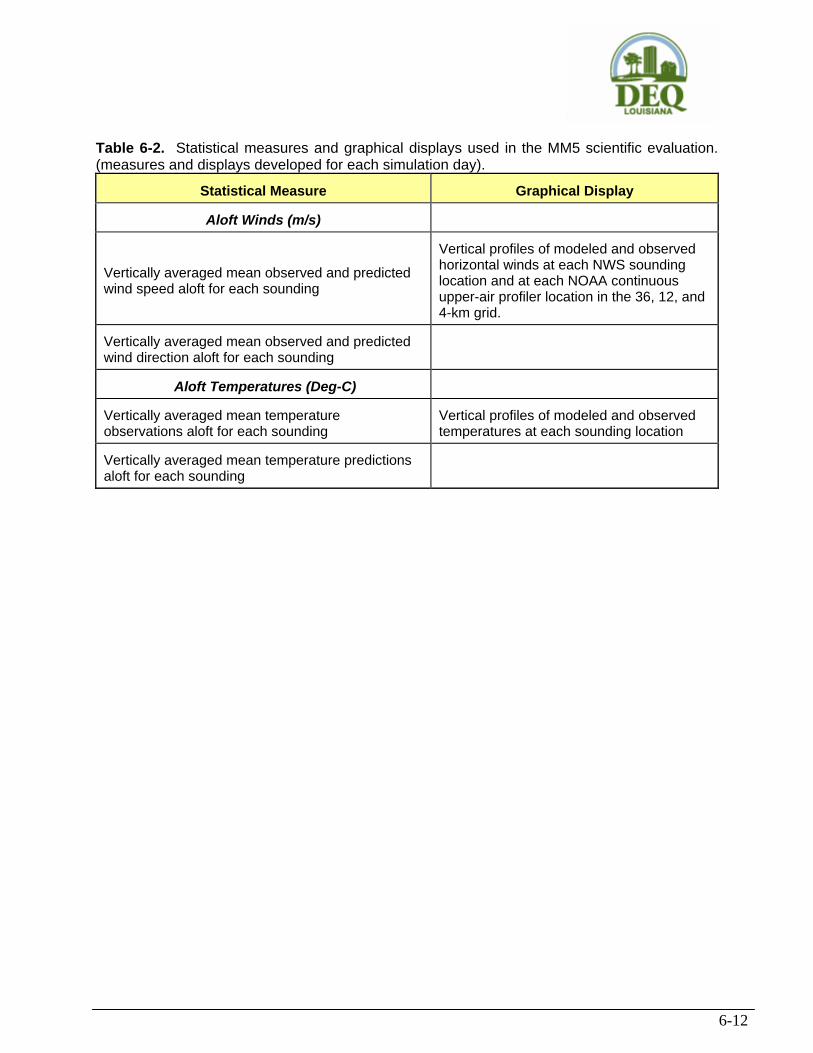
6-12

Table 6-2. Statistical measures and graphical displays used in the MM5 scientific evaluation. (measures and displays developed for each simulation day).

Statistical Measure

Graphical Display

Aloft Winds (m/s)

Vertically averaged mean observed and predicted wind speed aloft for each sounding

Vertical profiles of modeled and observed horizontal winds at each NWS sounding location and at each NOAA continuous upper-air profiler location in the 36, 12, and 4-km grid.

Vertically averaged mean observed and predicted wind direction aloft for each sounding

Aloft Temperatures (Deg-C)

Vertically averaged mean temperature observations aloft for each sounding

Vertical profiles of modeled and observed temperatures at each sounding location

Vertically averaged mean temperature predictions aloft for each sounding

6-13

Table 6-3. Statistical measures and graphical displays for 1-hour and 8-hour ozone concentrations to be used in the screening model performance evaluation (SMPE) of CAMx surface ozone concentrations.

Statistical Measure on 36/12/4 km grids

Graphical Display on all grids

Maximum observed concentration

Modeled and observed spatial mean concentrations as a function of time

Maximum modeled concentration

Measures of peak estimation accuracy (ATS, AT, AS, AU, A)

Maximum modeled concentration at a monitoring station

Normalized bias as a function of time

Ratio of maximum modeled to observed concentrations

Normalized gross error as a function of time

Accuracy of peak estimation (paired in time and space)

Normalized bias as a function of concentration level

Accuracy of peak estimation (unpaired in time and space)

Normalized gross error as a function of concentration level

Average accuracy over all stations

Scatterplot of hourly concentration pairs

Normalized bias in hourly concentrations

Scatterplot of daily maximum concentration pairs

Mean bias in hourly concentrations

Quartile plots of hourly species concentrations

Normalized gross error in hourly concentrations

Daily maximum ground-level concentration isopleths

Mean gross error in hourly concentrations

Variance in hourly concentrations

6-14

Table 6-4. Statistical measures and graphical displays for 1-hour and 8-hour ozone, VOCs, NOx, and indicator species and indicator species Ratios to be used in the refined model performance evaluation (RMPE) involving multi-species, multi-scale evaluation of CAMx surface and aloft concentrations.

Statistical Measure on 36/12/4 km grids

Graphical Display on all grids

Maximum observed concentration

Modeled and observed spatial mean concentrations as a function of time

Maximum modeled concentration

Measures of peak estimation accuracy (ATS, AT, AS, AU, A)

Maximum modeled concentration at a monitoring station

Normalized bias as a function of time

Ratio of maximum modeled to observed concentrations

Normalized gross error as a function of time

Accuracy of peak estimation (paired in time and space)

Normalized bias as a function of concentration level

Accuracy of peak estimation (unpaired in time and space)

Normalized gross error as a function of concentration level

Average accuracy over all stations

Scatterplot of hourly concentration pairs

Normalized bias in hourly concentrations

Scatterplot of daily maximum concentration pairs

Mean bias in hourly concentrations

Quartile plots of hourly species concentrations

Normalized gross error in hourly concentrations

Daily maximum ground-level concentration isopleths

Mean gross error in hourly concentrations

Variance in hourly concentrations

Mean, maximum, minimum, standard deviation, bias and error of observed and modeled aloft concentrations (e.g., ozone, NOx) along individual aircraft paths

Modeled and observed time series of ozone and NOx concentrations along individual aircraft flight paths

7-1

7.0 FUTURE YEAR MODELING This chapter discusses the future year modeling procedures to be performed by the LDEQ modeling team for the Baton Rouge ozone episodes that are shown to be performing adequately for use in 8-hour ozone attainment demonstration modeling. 7.1 Future Year to be Simulated Baton Rouge is currently designated a Marginal 8-hour ozone nonattainment area and so is required to achieve attainment by 2007. This means that the measured 8-hour ozone Design Values for the 2005-2007 period must all be less that 85 ppb. For modeling future-year attainment EPA guidance recommends that the mid-year from the 3-year Design Value attainment determination period be used which would be 2006. However, given the higher ozone measurements in recent years, Baton Rouge will not attain the 8-hour ozone standard by 2007. With a fourth highest 8-hour ozone standard at the LSU monitor in 2005 of 98 ppb, the fourth highest values at this monitor would have had to average 78 ppb for 2006 and 2007; measurements so far in 2006 show that this will not be possible. The next milestone 8-hour ozone attainment year is 2010, which will require that a 2009 future-year be modeled to ensure that the area fully attains by 2010. 7.2 Future Year Growth and Controls

Several RPOs, including CENRAP, VISTAS, WRAP and the MRPO, are refining future

year modeling inventories for 2009, 2012, and 2018 (Stella, 2004, 2005). EPA has developed future year inventories for 2010 and 2015 as part of their CAIR/CAMx analysis. The Texas Commission on Environmental Quality (TCEQ) has also developed future-year modeling inventories for their DFW and HGB ozone attainment efforts. Since the 36/12/4 km Baton Rouge modeling domain encompasses the inventories of several of these groups, projections developed by the RPOs, EPA and TCEQ may be the most appropriate starting point for use in future year modeling for the Baton Rouge modeling analysis region. These projections will cover the area, point, nonroad, and motor vehicle source categories. The LDEQ modeling team will review the appropriate datasets, with special attention to the 36/12/4 km Baton Rouge modeling domain, as these data become available.

Within Baton Rouge itself, developing growth factors will be particularly challenging.

Over the past year the population of Baton Rouge has approximately doubled in size due to the displacement of population from the Gulf Coast (e.g., New Orleans) caused by Hurricane Katrina, an event not forecast by current growth techniques (e.g., used by RPOs and EPA). This is an area of ongoing research that will have to be worked out during the course of the study with consultation among the LDEQ modeling team, local agencies, EPA and others.

7-2

7.2.1 Regional Growth and Control Factors

Coordinating with the CENRAP, MRPO, VISTAS, WRAP, MANE-VU, TCEQ and EPA, the modeling team will review and refine national and regional growth factors, MOBILE6 input files, and control program reduction estimates that are consistent with Baton Rouge’s definition of the future year 2009 base case for the attainment demonstration.

The files prepared will include all federally promulgated rules for the 36-km regional-

scale domain and will be largely based on data prepared by the RPOs (e.g., MRPO and VISTAS), States (e.g., Texas) and EPA. This information is based on the latest publicly available information from EPA’s federal rulemaking process and at the time of this writing are deemed to be the most recent information available on the topic. Each reviewed rule and regulation found applicable to the eastern U.S. modeling domain relevant to ozone abatement or visibility impairment will be documented with cite, geographic coverage, source categories of impact, and associated and expected emission reduction potential. Additional synchronization with EPA and CENRAP’s sister RPOs will be conducted to ensure consistent, if not comparable, application of these programs.

Using summary files prepared to present this information in an easily reviewable format,

the modeling team will contact individually identified or otherwise interested regional representatives to solicit comment on the originally presented growth and control factors. Upon review and comment of these factors, the team will revise the regional growth and control factors consistent with the comments collected. The control factor lists will then be compared to the base year emission inventory to determine which, if any, of these programs may already be accounted for in the emission estimates. The factors will be converted to create a complete set of EPS growth and control packets allowing the generation of future year controlled emissions. 7.2.2 Local Growth and Control Factors As noted above, the development of the Baton Rouge local growth and control factors will be particular challenging. Standard projection techniques that are used for other nonattainment areas (e.g., Economic Growth Analysis System, EGAS) are inappropriate for the Baton Rouge area, which has experienced very atypical growth patterns over the last year. The LDEQ modeling team will work with state and local agencies and EPA to develop appropriate and representative growth projections and control factors for the Baton Rouge area. 7.3 Future Model–Ready Emissions Inventory Development and QA

Future year emissions will be processed into the gridded speciated hourly three-dimensional emissions inputs for the CAMx photochemical model using the EPS3 emissions model. The same biogenic emissions as used in the Baton Rouge base year modeling will be used for the future-year modeling. This assumes that the same land use and biomass distribution as used in the base case emissions would exist in the future-year emission scenarios. The effects of changes in Baton Rouge landuse (growth), agriculture, deforestation, etc. between the current and future-year would not be included. If future-year travel demand model (TDM) link-based VMT data are available they will be used to generate on-road mobile source emissions for the

7-3

future year. Typical-year EGU and fire emissions (if fires were included in the base year emissions scenario) would also be used in the future-year.

Similar QA/QC will be performed on the future year model-ready emissions inventories as were utilized in checking the base year datasets. Standard inventory assessment methods will be employed to generate the future year emissions data including, but not limited to: (a) visualizing the model-ready emissions graphically, (b) spot-checking the holiday emissions files to confirm that they are temporally allocated like Sundays. (c) producing pie charts emission summaries for each source category, (d) normalizing the emissions by population for each state to reveal where the future year inventories may be suspect and (e) spot-checks of the vertical allocation of point sources using PAVE. The additional QA analyses and reports that we may find particularly useful for the future year emissions files are given in Section 5.2.4. 7.4 Future Year Baseline Air Quality Simulations

The Baton Rouge future-year modeling will use the MM5 meteorological conditions

developed for the Baton Rouge ozone episodes. That is, the meteorological conditions for the future-year are assumed to be the same as for base year ozone episodes. This will allow for the comparison of the changes in 8-hour ozone concentrations in the study area from the current to future-year due to changes in emissions only. This means that the effects of inter-annual variability, land use variations and climatic variations will not be accounted for in the future-year meteorological inputs. Several other decisions concerning the future-year to be modeled, model(s) to be used, and modifications to the model inputs to reflect future years, need to be made, as described below. 7.4.1 Future-Year Initial and Boundary Conditions

The same initial conditions as used in the base year would be used in the future-year modeling. Because a 10 day spin up period is being used, initial conditions should have minimal if any influence on the model estimated concentrations.

The base year boundary conditions will be developed from the CENRAP 2002 base case

simulation on the national RPO 36-km grid (see Section 5.3.1). If appropriate similar future-year simulations are also available, then they will be processed the same way as the base year. Otherwise, the 2002 boundary conditions will be held constant for the future-year modeling. 7.4.2 Other Future-Year Modeling Inputs

All other future-year CAMx modeling inputs will be identical to the base year simulation, including meteorology, photolysis rates, landuse, and other inputs. 7.5 Emissions Sensitivity Experiments Model sensitivity experiments are a vital and mandatory component of an 8-hour ozone SIP attainment demonstration analysis – both for the base case performance assessment (see Chapter 6) as well as in the future year control strategy assessment and uncertainty analysis.

7-4

Turning specifically to the future year assessments, sensitivity analyses are designed to facilitate the emissions control scenario identification and evaluation process. Today, four complimentary “Probing Tools” can be used in the CAMx regional photochemical model. These methods include: (a) traditional or “brute force” testing, (b) the direct decoupled method (DDM), (c) Ozone Source Apportionment Technology (OSAT), and (d) Process Analysis (PA). The LDEQ modeling team may use at least two types of emissions sensitivity testing methods with the CAMx future year simulations.

Traditional Sensitivity Testing: The LDEQ modeling team may perform numerous sensitivity runs to explore response to emissions changes as well as changes in key input parameters. Typically, these sensitivity runs entail scalar reductions to key categories of anthropogenic emissions (e.g., 20% reduction in on-road motor vehicle emissions, 20% reduction in emissions from elevated point sources, 20% reduction in architectural coating VOC emissions, etc.). These sensitivity runs serve two purposes. They: (a) aid in helping to define more refined emissions control scenarios, and (b) they provide episode-specific model uncertainty information that may be used later in the “Weight of Evidence” analyses in support of the 8-hour ozone attainment demonstrations. DDM Sensitivity Modeling: Another type of sensitivity modeling entails the use of the Direct Decoupled Method (DDM) technology in CAMx. For one or more episodes, the DDM algorithm may be exercised to produce a numerically intensive, direct sensitivity/uncertainty analysis. These future year DDM sensitivity simulations are an adjunct to the brute force runs and also help to design future year, realistic ozone control strategies, as needed, for the Baton Rouge region.

Ozone Source Apportionment: With CAMx, focused use of ozone source apportionment technology (OSAT) for selected future-year episodes may be employed to better understand model response and to aid in the design of control strategies. The value of source apportionment modeling for subsequent stages of the Baton Rouge modeling study is that these calculations will help to: (a) assess the contribution of sources in the Louisiana region and surrounding states to ozone concentrations in key receptor areas in the Baton Rouge area, and (b) identify the particular source categories that may contribute the most to future-year elevated 8-hour ozone concentrations at various nonattainment monitors.

7.6 Control Strategy Development, Testing and Analysis

The general approach to be followed in assessing whether the Baton Rouge region is likely to be in attainment of the 8-hour ozone standard or whether and to what extent additional VOC and NOx emissions reductions will be required to achieve attainment will be consistent with the methodologies stipulated in EPA’s recent 8-hour ozone modeling guidance (EPA, 2005a). The procedure to be followed in performing the ozone attainment demonstrations is discussed in Chapter 8. The main theme of this approach is to use the model in a relative sense through model-derived site-specific relative reduction factors (RRFs) that are used to scale the observed 8-hour ozone Design Values (DVs).

7-5

The CAMx 2009 future-year 8-hour ozone simulations will reveal the extent to which further emissions reductions are needed in the region to provide for attainment of the 8-hour ozone NAAQS by 2010. Should ozone violations be projected in the region in the future year simulation, the severity, location, and spatial extent of the modeled exceedances will be studied in order to postulate candidate emissions reductions strategies within and upwind of the nonattainment area. That is, should the future year modeling reveal a nonattainment problem, then an attainment demonstration analysis will be performed that will include the 8-hour ozone modeled attainment test, specific screening analysis and supplemental corroborative analyses set forth in the EPA guidance. These attainment demonstration procedures for ozone are described in detail in the following Chapter 8.

It is difficult when a modeling study protocol is first prepared to specify precisely the nature of the future year local and regional ozone control scenarios that may be required; indeed, the application of existing and mandated regional and local controls “on the books” and “on the way” (e.g., the effects of the Clean Air Interstate Rule) will potentially and dramatically change the current attainment picture in the region.

8-1

8.0 OZONE ATTAINMENT DEMONSTRATION The ultimate objective of the Baton Rouge modeling study is the development of modeling databases that can be used to define emissions control strategies that demonstrate future-year attainment of the 8-hour ozone National Ambient Air Quality Standard (NAAQS). This section describes the procedures for demonstrating future-year attainment of 8-hour ozone NAAQS. 8.1 Ozone Weight of Evidence Analyses A central theme of EPA’s 8-hour ozone modeling guidance document is the use of supporting corroborative analyses to bolster confidence that the selected control plan will in fact achieve attainment in the future-year (EPA, 2005a). This corroborative analysis is part of the Weight of Evidence (WOE) used in a State Implementation Plan (SIP) to support the final control plan selection. Details of the WOE and types of corroborative analysis that can be used in an ozone attainment demonstration have been discussed earlier in Chapter 1. 8.2 8-Hour Ozone Attainment Demonstration Procedures The procedures for performing a modeled ozone attainment demonstration are outlined in EPA’s 8-hour ozone modeling guidance (EPA, 2005a). These procedures involve the use of the model in a relative sense to scale the observed site-specific 8-hour ozone Design Values based on the relative changes in the modeled 8-hour ozone concentration between the current-year (e.g., 2002-2005) and 2009 future-year. The model-derived scaling factors are called Relative Reduction Factors (RRFs). The general procedures are as follows:

• Start with the average of three 3-year periods of 8-hour ozone Design Values centered on either 2002 or 2003 (i.e., average either of the 2000-2002, 2001-2003 and 2002-2004 8-hour ozone Design Values at each ozone monitor in Baton Rouge, or average the three years of 2001-2003, 2002-2004 and 2003-2005, to be determined with consultation with EPA);

• Perform base year modeling on the 36/12/4 km grid for the selected Baton Rouge ozone episodes;

• Perform 2009 future-year base case and control strategy modeling on the 36/12/4 km grid for the ozone episodes;

• Develop RRFs, defined as the ratio of the average of 8-hour daily maximum ozone concentrations “near” each monitor for the future year emission scenarios and the base year for all ozone values above a “threshold” value: o Here, “near” the monitor is defined as a 3x3 or 5x5 array of 4-km grid cells

centered on the ozone monitor (as much as a 7x7 array is recommended, but the monitoring sites are grouped rather closely in Baton Rouge, necessitating the need for a smaller number of grid cells to avoid overlap with other monitors);

o EPA’s 8-hour ozone guidance specifies that RRFs should be calculated using all days with base-year ozone concentrations near the monitor greater or equal to 85

8-2

ppb, and also recommends that at least 10 modeling days should be included – these two recommendations may be in conflict: • In the event that there are less than 10 modeling days with base year daily

maximum 8-hour ozone concentrations near the monitor > 85 ppb threshold then: • The threshold is successively reduced by 1 ppb (e.g., 84 ppb, 83 ppb, etc.)

until 10 modeling days are obtained; or • A 70 ppb threshold floor is imposed;

• If there are still less than 10 days upon reaching the 70 ppb threshold then: • If there are 5 or more days, proceed with the attainment demonstration but

the results should be analyzed carefully to be sure no single day is producing unusual model signals; or

• If there are less than 5 days EPA Region 6 will be contacted for advice; • Apply the modeled-derived RRFs to the three-year average of observed 8-hour ozone

Design Values at each ozone monitor to obtain a projected future year 8-hour ozone Design Value;

• Compare the projected 8-hour ozone at each monitor with the 8-hour ozone standard, where if all projected 8-hour ozone values are 84.9 ppb or lower then attainment has been demonstrated;

• Even if the modeled future-year 8-hour ozone Design Value is 85 ppb or higher, a WOE attainment demonstration may be possible using supportive, corroborative and additional analysis: o In fact, EPA recommends that the WOE analysis be conducted with projected 8-

hour ozone Design Values in the 82 to 87 ppb range; o EPA notes that for projected 8-hour ozone Design Values of 88 ppb or higher no

amount of supportive information would likely be convincing for an attainment demonstration.

R-1

REFERENCES Abraczinskas, M., D.T. Olerud, and A.P. Sims. 2004. Characterizing annual meteorological

modeling performance for visibility improvement strategy modeling in the southeastern U.S. 13th AMS Joint Conf. on Applications of Air Pollution Meteorology with the Air & Waste Manage. Assoc. American Meteoro. Society, Vancouver, BC.

Anthes, R.A. 1977. “A Cumulus Parameterization Scheme Utilizing a One-Dimensional Cloud

Model”, Mon. Wea. Rev., Vol. 105, pp. 270-286. Anthes, R.A. and T.T. Warner. 1978. “The Development of Mesoscale Models Suitable for Air

Pollution and Other Mesometeorological Studies”, Mon. Wea. Rev., Vol. 106, pp, 1045-1078.

Arnold, J.R., R.L. Dennis, and G.S. Tonnesen. 2003. “Diagnostic Evaluation of Numerical Air

Quality Models with Specialized Ambient Observations: Testing the Community Multiscale Air Quality Modeling System (CMAQ) at Selected SOS 95 Ground Sites”, Atmos. Environ., Vol. 37, pp. 1185-1198.

Barchet, W.R., and R.L. Dennis. 1990. “ANAPAP Model Evaluation, Volume 1: Protocol”,

prepared for the U.S. Environmental Protection Agency, prepared by Battelle Pacific Northwest Laboratories, Richland, WA.

Byun, D. W., et al. 2005a. “Parallel Computation of the Air Quality Forecasting System for Eastern

Texas”, prepared by the Institute for Multidimensional Air Quality Studies (IMAQS)-University of Houston, April.

Byun, D. W., et al. 2005b. “Development and Operational Evaluation of the Eastern Texas Air

Quality (ETAQ) Forecasting System Based on MM5/SMOKE/CMAQ”, presented at the 4th Annual CMAS Models-3 User's Conference, University of North Carolina, Chapel Hill, NC. 26-28. http://cf.cmascenter.org/html/2005_conference/conf_agenda.cfm

Coe D. and S. Reid. 2003. “Research and Development of Ammonia Emission Inventories for the

Central States regional Air Planning Association”. Final Report. Sonoma Technology, Inc. (STI). October 30.

Diggs T.H. 2005. U.S. Environmental Agency (EPA) Region 6 Detailed Comments on the Draft

Modeling Protocol for the Baton Rouge Area. Letter from Thomas H. Diggs, Chief Air Planning Section, U.S. EPA Region 6 to Mr. Chris Roberie, Administrator, Air Quality Assessment Division, Louisiana Department of Environmental Quality, Baton Rouge, LA. July 29.

Dudhia, J. 1993. "A Non-hydrostatic Version of the Penn State/NCAR Mesoscale Model:

Validation Tests and Simulation of an Atlantic Cyclone and Cold Front", Mon. Wea. Rev., Vol. 121. pp. 1493-1513.

R-2

Emery, C. et al. 1999. “Ozone Modeling for the Kansas City Nonattainment Area: Final Protocol”, prepared for the Kansas Department of Health and Environment, prepared by ENVIRON International Corporation and Alpine Geophysics.

Emery, C., E. Tai, and G. Yarwood. 2001. “Enhanced Meteorological Modeling and Performance

Evaluation for Two Texas Episodes”, report to the Texas Natural Resources Conservation Commission, prepared by ENVIRON, International Corp, Novato, CA.

ENVIRON. 2004. User’s Guide – Comprehensive Air-quality Model with extensions, Version

4.10s. ENVIRON International Corporation, Novato, California. (http://www.camx.com). ENVIRON and UCR. 2004. “Modeling Protocol for the CENRAP 2002 Annual Emissions and Air

Quality Modeling.” ENVIRON International Corporation and University of California at Riverside. November 19.

ENVIRON. 2006. User’s Guide – Comprehensive Air Quality Model with Extensions – Version

4.30. ENVIRON International Corporation, Novato, California (www.camx.com). February.

EPA. 1990. Users Guide for the Urban Airshed Model, Volume IV: User’s Manual for the

Emissions Preprocessor System, Version 2.0, Part A: Core Fortran System. U.S. Environmental Protection Agency, Research Triangle Part, NC.

EPA. 1991. "Guidance for Regulatory Application of the Urban Airshed Model (UAM), "Office of

Air Quality Planning and Standards, U.S. Environmental Protection Agency, Research Triangle Park, N.C.

EPA. 1999. “Draft Guidance on the Use of Models and Other Analyses in Attainment

Demonstrations for the 8-hr Ozone NAAQS”. Draft (May 1999), U.S. Environmental Protection Agency, Office of Air Quality Planning and Standards, Research Triangle Park, N.C

EPA. 2001. “Guidance Demonstrating Attainment Air Quality Goals for PM2.5 and Regional

Haze”. Draft Final (17 February 2005), U.S. Environmental Protection Agency, Atmospheric Sciences Modeling Division, Research Triangle Park, N.C.

EPA. 2001. “Guidance for Demonstrating Attainment of Air Quality Goals for PM2.5 and Regional Haze”, Draft Report, U.S. Environmental Protection Agency, Research Triangle Park, NC.

EPA. 2005a. Guidance on the Use of Models and Other Analyses in Attainment Demonstrations for the 8-hr Ozone NAAQS -- Final. U.S. Environmental Protection Agency, Atmospheric Sciences Modeling Division, Research Triangle Park, N.C. October.

EPA. 2005b. Technical Support Document for the Final Clean Air Interstate Rule – Air Quality

Modeling. U.S. Environmental Protection Agency, Office of Air Quality and Planning Standards, Research Triangle Park, North Carolina, 27711. March.

R-3

EPA. 2005c. “Regional Haze Regulations and Guidelines for Best Available Technology

(BART) Determinations”. Fed. Reg./Vol. 70, No. 128/Wed. July 6, 2005, Rules and Regulations, pp. 39104-39172. 40 CFR Part 51, FRL-7925-9, RIN AJ31.

Fahey, K.M., and S.N. Pandis. 2001. Optimizing model performance: variable size reduction in

cloud chemistry modeling. Atmos. Environ. Vol. 35, pp. 4471-4478. Gery, M. W., G.Z. Whitten, J.P. Killus, and M.C. Dodge. 1989. A photochemical mechanism for

urban and regional-scale computer modeling. J. Geophys. Res. 94, 12925-12956. Green M., J. Watson, H. Kuhns, R. Morris, A. Pollack, P. Fields and M. Wolf. 2002. “A Scoping

Study for Haze in the CENRAP Region”. Final Report. Desert Research Institute (DRI), EBVIRON and ERG. December 18.

Grell, G. A., J. Dudhia, and D. R. Stauffer. 1994. "A Description of the Fifth Generation Penn

State/NCAR Mesoscale Model (MM5). NCAR Tech. Note, NCAR TN-398-STR, 138 pp. Gao, Y.-R., Y.-H. Kuo, J. Dudhia, and D.B. Barsons. 2000. Four-dimensional variational data

assimilation of heterogeneous mesoscale observations for a strong convective case. Mon. Wea. Rev., 128, 619-643.

ICF. 2005. 8-Hour Modeling Analysis for the Baton Rouge 5-Parish Area – Draft Technical

Protocol. ICF Consulting, Systems Applications International, LLC, 101 Lucas Valley Road, Suite 260, San Rafael, CA 94903. June 14.

Johnson, M. 2004. “Annual 2002 MM5 v363 Simulation Evaluation.” Iowa Department of natural

Resources, Air Quality Bureau. November. (Available at www.ladco.org/tech/photo/present/mm5v363_eval.pdf).

Kemball-Cook, S. Y Jia, C. Emery, R. Morris, Z. Wang, G. Tonnesen. 2004. 2002 Annual

MM5 Simulation to Support WRAP CMAQ Visibility Modeling for the Section 308 SIP/TIP: MM5 Sensitivity Simulations to Identify a More Optimal MM5 Configuration for Simulating Meteorology in the Western United States. Prepared for the Western Regional Air Partnership, by ENVIRON International Corporation and UC Riverside, CE-CERT. December 20, 2004.

Morris, R. E. and T. C. Myers. 1990. “User's Guide for the Urban Airshed Model. Volume I: User's Manual for UAM (CB-IV)” prepared for the U.S. Environmental Protection Agency (EPA-450/4-90-007a), Systems Applications International, San Rafael, CA.

Morris, R. E., M. A. Yocke, T. C. Myers, and R. C. Kessler. 1991. “Development and Testing

of a Nested-Grid Version of the Urban Airshed Model UAM-V” paper presented at the Air and Waste Management Association Specialty Conference: Tropospheric Ozone and the Environment II, Atlanta, GA. November.

R-4

Morris, R.E., B. Koo, S. Lau, T.W. Tesche, D. McNally, C. Loomis, G. Stella, G. Tonnesen and Z. Wang. 2004. “VISTAS Emissions and Air Quality Modeling – Phase I Task 4cd Report: Model Performance Evaluation and Model Sensitivity Tests for Three Phase I Episodes”, prepared for the VISTAS Technical Analysis Committee, prepared by ENVIRON International Corporation, Alpine Geophysics, LLC, and the University of California, Riverside (CE-CERT).

Morris, R.E., D. McNally, T. Tesche, G. Tonnesen, J. Boylan and P. Brewer. 2004. “Regional

Haze Modeling over the VISTAS States: Preliminary Verification of Models-3/CMAQ for the 2002 Annual Period.” Presented at AWMA Visibility Conference, Asheville, North Carolina. October.

Morris, R.E., A. Hoats, S. Lau, B. Koo, G. Tonnesen, C-J. Jung and M. Omary. 2005c. Air Quality

Modeling Analysis for CENRAP – Preliminary 2002 Base Case CMAQ and CAMx Modeling of the Continental US 36 km Domain and Model Performance Evaluation. ENVIRON International Corporation, Novato, CA. April.

Morris R.E., E. Tai, Y. Jia and M. Jimenez. 2005d. Photochemical Modeling of the Tulsa and

Oklahoma City 8-Hour Ozone Early Action Compact (EAC) State Implementation Plan (SIP) – Technical Support Document. ENVIRON International Corporation, Novato, California. March 28.

Morris R.E. and G. Tonnesen. 2006. Quality Assurance Project Plan (Draft) for Central Regional

Air Partnership (CENRAP) Emissions and Air Quality Modeling – Revision 3. ENVIRON International Corporation, Novato, California. March 29.

Nenes, A., C. Pininis, and S.N. Pandis. 1998. ISORROPIA: A New Thermodynamic Model for

Multiphase Multicomponent Inorganic Aerosols. Aquatic Geochemistry, 4, 123-152. Nenes, A., C. Pininis, and S.N. Pandis. 1998. Continued Development and Testing of a New

Thermodynamic Module for Urban and Regional Air Quality Models. Atmos. Environ., 33, 1533-1560.

Nielsen-Gammon, J. W., R.T. McNider, A.B. White, W. Angevin, and K. Nnupp. 2005. Mesoscale

model performance with assimilation of wind profiler data: Sensitivity to assimilation parameters and network configuration. J. Appl. Meteorol,. (in press).

Olerud, D. and A. Sims. 2004a. “Protocol for Annual MM5 Sensitivity Modeling in Support of

VISTAS (Visibility Improvement - State and Tribal Association)] VISTAS Task 3a deliverable”. Available from Mike Abraczinskas, Meteorologist, NC Division of Air Quality, 1641 Mail Service Center, Raleigh, NC 27699-1641

Olerud, D. and A. Sims. 2004b. MM5 2002 Modeling in Support of VISTAS (Visibility

Improvement – State and Tribal Association). Baron Advanced Meteorological Systems, LLC, Research Triangle Park, NC. (http://www.baronams.com/projects/VISTAS/).

R-5

Pilinis, C., K.P. Capaldo, A. Nenes, and S.N. Pandis. 2000. “MADM - A new multicomponent aerosol dynamics model.” Aerosol Sci. Tech., Vol. 32(5), pp. 482-502. 2000.

Pitchford, M.L., I. Tombach, M. Barna, K. Gebhart, M. Green, E. Knipping, N. Kumar, W. Malm,

B. Pun, N. Schichtel and C. Seigneur. 2004. “Big Bend Aerosol and Visibility Study”. Final Report. September.

Pun B., S-Y. Chen and C. Seigneur. 2004. “CENRAP Model Simulations and Performance

Evaluations”. Atmospheric and Environmental Research, Inc. (AER). August. Reid S., S. Brown, D. Sullivan, H. Arkinson, T. Funk, and P. Stiefer. 2004a. “Research and

Development of Planned Burning Emission Inventories for the Central States Regional Air Planning Association”. Final Report. Sonoma Technology, Inc. (STI). July 30.

Reid, S., D. Sullivan, B. Penfold, T. Funk, T. Tamura, P. Stiefer, S. Raffuse and H. Arkinson. 2004.

“Emission Inventory Development for Mobile Sources and Agricultural Dust Sources form the Central States”. Final Report. Sonoma Technology, Inc. (STI). September 22.

Reynolds, S. D., C.L., Blanchard, S.D., Ziman. 2003. Understanding the effectiveness of precursor

reductions in lowering 8-hr ozone concentrations. Journal of the Air & Waste Manage. Association, 53, 195-205.

Roth, P.M., S.D. Reynolds, and T.W. Tesche. 2005. Air quality modeling and decisions for ozone

reduction strategies. Journal of the Air & Waste Manage. Association, 56, 1-16. Russell, A.G., and R.L. Dennis. 2000. “NARSTO Critical Review of Photochemical Models and

Modeling”, Atmos. Environ., Vol. 34, No. 12-14, pp. 2283-2324. Seaman, N.L. 1995. “Status of Meteorological Pre-Processors for Air Quality Modeling”,

International Conf. On Particulate Matter, Air and Waste Mgt. Assn., Pittsburgh, PA. Seaman, N.L. 1995. “Status of Meteorological Pre-Processors for Air Quality Modeling”,

International Conf. On Particulate Matter, Air and Waste Mgt. Assn., Pittsburgh, PA. Seaman, N.L. 1996. “Study of Meteorological Variables Needed in Air-Quality Modeling’, Annual

Progress Report prepared for the Coordinating Research Council (CRC), Interim Report, Project A-11, prepared by the Department of Meteorology, Penn State University, State College, PA.

Seaman, N.L. 2000. “Meteorological Modeling for Air Quality Assessments”, Atmos. Environ.,

Vol. 34, No. 12-14, 2231-2260. Seaman, N. L., and D. R. Stauffer. 1996. "SARMAP Meteorological Model Final Report",

prepared for the San Joaquin Valleywide Air Pollution Study Agency, prepared by the Department of Meteorology, Pennsylvania State University, University Park, PA.

R-6

Seaman, N.L., D.R. Stauffer, and T.W. Tesche. 1992. "The SARMAP Meteorological Model: A Four-Dimensional Data Assimilation Technique Used to Simulate Mesobeta-Scale Meteorology During a High-Ozone Episode in California", International Specialty Conference on Tropospheric Ozone Nonattainment and Design Value Issues, U.S. EPA/AWMA, 27-30 October, Boston, MA.

Seaman, N.L., D.R. Stauffer, and L.M. Lario. 1995. "A MultiScale Four-Dimensional Data

Assimilation System Applied to the San Joaquin Valley During SARMAP. Part I: Modeling Design and Basic Performance Characteristics", J. Appl. Meteo., Vol. 34, pp. 1739-1761.

Seaman, N.L., D.R. Stauffer, and D.E. McNally. 1996. "Application of the MM5-FDDA

Meteorological Model to the Southern California SCAQS-1997 Domain: Preliminary Test Using the SCAQS August 1987 Case", Ninth Joint Conference on Applications of Air Pollution Meteorology, American Meteorological Society, 28 January-2 February, Atlanta, GA.

Sistla, G., W. Hao, J-Y Ku, G. Kallos, K. Zhang, H. Mao, and S.T. Rao. 2001. An operational

evaluation of two regional-sale ozone air quality modeling systems over the eastern United States. Bull. Amer. Meteorological Soc., 82, (5), 945-964.

Stauffer, D.R. and N.L. Seaman. 1990. “Use of Four-Dimensional Data Assimilation in a Limited-

Area Mesoscale Model. Part I: Experiments with Synoptic Data”. Mon. Wea. Rev., 118, 1250-1277.

Strader, R., F.W. Lurmann and S.N. Pandis. 1999. “Evaluation of secondary organic aerosol

formation in winter.” Atmos. Environ. Vol. 33, pp. 4849-4864. Strait, R., S. Roe and J. Vukovich. 2004. “2002 Base Case Modeling Inventory – Work Plan.”

E.H. Pechan and Associates, Inc. Durham, North Carolina. July 30. Tesche, T.W., and D.E. McNally. 1993a. “Operational Evaluation of the CAL-RAMS

Meteorological Model for LMOS Episode 1: 26-28 June 1991", prepared for the Lake Michigan Air Directors Consortium, prepared by Alpine Geophysics, LLC, Crested Butte, CO.

Tesche, T.W. and D.E. McNally. 1996b. “Superregional Ozone Modeling and Analysis Study C

Phase II: Work Element 5 Technical Report: Comparative Evaluation of the MM5 and RAMS Models for the July 1991 OTAG Episode”, prepared for the Midwest Ozone Group, prepared by Alpine Geophysics, LLC, Ft. Wright, KY.

Tesche, T.W., et al. 2002. “Operational Evaluation of the MM5 Meteorological Model over the

Continental United States: Protocol for Annual and Episodic Evaluation”, prepared for the U. S. Environmental Protection Agency, Office of Air Quality Planning and Standards, prepared by Alpine Geophysics, LLC, Ft. Wright, KY.

R-7

Tesche, T.W., and H.E. Jeffries. 2002. “Findings From BCCA-AG Science Studies”, prepared for the Business Coalition for Clean Air- Appeals Group, (2002), prepared by Alpine Geophysics, LLC, Ft. Wright, KY.

Tesche, T.W., R.E. Morris, G. Tonnesen, D.E. McNally, J. Boylan, and P. Brewer. 2005a .

CMAQ/CAMx Annual 2002 Performance Evaluation over the Eastern U.S. Atmospheric Environment (in press).

Tesche, T.W., D.E. McNally, C.F. Loomis, G.M. Stella, and J.G. Wilkinson. 2005b. “Modeling

Support for the Houston 8-hr Ozone Attainment Demonstration: 8-Hr Ozone Modeling Protocol”, prepared for the Houston 8-hr Ozone Coalition and the Texas Commission on Air Quality, prepared by Alpine Geophysics, LLC, Ft. Wright, KY.

Tonnesen, G., R.E. Morris, J. Vimont, M. Uhl, K. Briggs and T. Moore. 2003. “The WRAP

Regional Modeling Center – Application and Evaluation of Regional Visibility Models.” Presented at AWMA Annual Meeting and Exhibition. June.

Wesely, M.L. 1989. Parameterization of Surface Resistances to Gaseous Dry Deposition in

Regional-Scale Numerical Models. Atmos. Environ., 23, 1293-1304. Xiu, A. and J.E. Pleim. 2000. Development of a land surface model. Part I: application in a

mesoscale meteorology model. J. App. Met., 40, pp. 192-209.

A-1

APPENDIX A

Quality Assurance Project Plan

A-2

A.0 QUALITY ASSURANCE PROJECT PLAN In this appendix we discuss the quality assurance procedures that will be used in the Baton Rouge 8-hour ozone modeling study. These procedures follow EPA’s recommendations for a Quality Assurance Project Plan (QAPP). A.1 Quality Assurance Objectives In December 2002, the USEPA publish extensive guidance on developing a Quality Assurance Project Plan (QAPP) for modeling studies (EPA, 2002). The objective of a QAPP is to ensure that a modeling study is scientifically sound, robust, and defensible. The new EPA guidance suggests that a QAPP should include the following elements:

• A systematic planning process including identification of assessments and related performance criteria;

• Peer reviewed theory and equations; • A carefully designed life-cycle development process that minimizes errors; • Clear documentation of assumptions, theory, and parameterization that is detailed enough

so others can fully understand the model output; • Input data and parameters that are accurate and appropriate for the problem; • Output data that can be used to help inform decision making; and • Documentation of any changes from the original quality assurance plan.

Moreover, the EPA guidance specifies that different levels of QAPP may be required depending on the intended application of the model, with a modeling study designed for regulatory purposes requiring the highest level of quality assurance. The QAPP also provides a valuable resource for project management. It can be used to document data sources and assumptions used in the modeling study, and it can be used to guide project personnel through the data processing and model application process to ensure that choices are consistent with the project objectives. The guidance document also addresses model development, coding and selection of models, and model performance requirements. For the Baton Rouge ozone study, the LDEQ is using existing models (MM5, EPS and CAMx) with a demonstrated past history of successful application throughout the U.S. and abroad; LDEQ has no current plans for model development activities. Thus, our QAPP focuses primarily on documenting data sources and QA of data processing performed by the modeling team. QA objectives for specific aspects of the project are discussed below, and these will be incorporated into a QAPP that conforms to the EPA guidance documents for modeling studies (e.g., EPA, 1991; 1999; 2005a).

A-3

A.2 QA for the Baton Rouge 8-hour Ozone Modeling

The Baton Rouge modeling study will use emissions data sets provided by the RPOs, States, and EPA, and will generate MM5 meteorological data for the Baton Rouge 8-hour ozone modeling episodes. Closely integrated with the episodic meteorological, emissions and air quality modeling will be ongoing project management, technical review, and QA activities performed under the guidance of the LDEQ technical staff. Complementing the data acquisition, modeling input development activities, and project management activities, the following QA activities/functions will be performed, consistent with this QAPP and the study Modeling Protocol. A.2.1 Data Gatekeeping

The modeling team will receive emissions, meteorological, and air quality data from the RPOs, States, EPA and others. As a first line of QA, the LDEQ modeling team will perform a gatekeeping function to assure: (a) that the emissions, meteorological and air quality data provided to the modeling team have been received correctly from their original data repositories, (b) that the data have been evaluated for quality and consistency, and (c) that the data received have been properly documented and logged. Separate air quality, meteorological and emissions gatekeeper functions by the LDEQ modeling team are defined below.

Air Quality Data Gatekeeper: An Air Quality Data Gatekeeper appointed by the LDEQ is responsible for obtaining and reviewing air quality data as appropriate for model input development and model performance evaluation and for assuring that the quality of all air quality data obtained are consistent with the approved QAPP. The LDEQ air quality data gatekeeper is responsible for providing documentation of the quality of the aerometric data sets to be used by the modeling team in preparing inputs for CAMx for all modeling runs and for the various simulation performance evaluations. Meteorological Gatekeeper: The LDEQ will appoint a Meteorological Gatekeeper who will be responsible for obtaining and/or developing the meteorological data used to exercise the MM5 model and to develop emissions and air quality model inputs for the CAMx simulations of the Baton Rouge 8-hour ozone modeling episodes. The meteorological gatekeeper function also performs data quality checks as approved in the QAPP, together with the appropriate documentation of model performance evaluation activities. Emissions Gatekeeper: The Emissions Gatekeeper is responsible for obtaining the emissions inventory data to be used in the Baton Rouge modeling study to support episodic current and future year modeling and recommend sources of emissions data to be used. The emissions gatekeeper assures quality of all emissions data received are consistent with the approved QAPP, and develops all emissions modeling files to support the modeling runs. Data Management Gatekeeper: The LDEQ is responsible for maintaining a modeling website and or ftp site including posting modeling input and output files, reports, interpretation of results, and other documents developed the modeling team. This includes, for example, the storage of model inputs and outputs for annual (and episodic) runs and the transfer (via fire wire or alternative media) of electronic files to EPA, other participants, and stakeholders. The timely and continuous involvement of the EPA in the development of the Baton Rouge 8-hour ozone attainment plan is an important component of the study.

A-4

A.2.2 Emissions QA/QC

Emissions Quality Assurance (QA) and Quality Control (QC) are some of the most critical steps in performing air quality modeling studies. Because emissions processing is tedious, time consuming and involves complex manipulation of many different types of large data sets, errors are frequently made in emissions processing and, if rigorous QA measures are not in place, these errors may remain undetected. The LDEQ emissions gatekeeper will perform a multistep emissions QA/QC approach. This includes the initial emissions QA/QC as described above, as well as QA/QC by the modeling team. The team’s QA/QC will occur largely during the processing of emissions, followed by additional QA/QC by the air quality modelers of the final CAMx-ready emissions. This multistep process with separate groups involved in the QA/QC of the emissions is designed to detect and correct errors prior to the air quality model simulations.

Emissions QA/QC performed as part of the emissions modeling includes:

EPA Input Screening Error Checking Algorithms: Although the EPS emissions model will be used for emissions processing and contains numerous internal QA/QC checks and reporting, some additional input error checking algorithms like those used with the EMS and SMOKE emission models may be considered to screen the data and identify potential emission input errors. Additionally, EPA has issued a revised stack QA and augmentation procedures memorandum that will be used to identify and augment any outlying stacks.

EPS Error Messages: EPS provides various cautionary or warning messages during the emissions processing. The user may redirect the EPS output to log files and review the log files for serious error messages. An archive of the log files will be maintained so that the error messages can be reviewed at a later date if necessary.

EPS Emissions Summaries: QA functions built into the EPS emissions processing system will be used to provide summaries of processed emissions as daily totals according to species, source category and county and state boundaries. These summaries will then be compared with summary data prepared for the pre-processed emissions (e.g., state and county totals for emissions from the augmented emissions data).

After the CAMx-ready emission inputs have been prepared, additional emissions QA/QC will

be performed as appropriate, such as:

Spatial Summary: Emissions are summed for each major source category and for all 24 hours and used to prepare PAVE plots showing the daily total emissions spatial distribution. In our base case simulations these plots will be presented as tons per day. The 5 emission categories typically used are biogenic, on-road mobile, non-road mobile, area and point sources. If possible, separate spatial QA plots will be generated for low-level and elevated point sources. The objective of this step is to identify errors in spatial distribution of emissions. In addition, daily summary plots are prepared for the total emissions summed across all source categories

Short Term Temporal Summary: The total domain emissions for each hour will be accumulated and time series plots prepared by source category that display the diurnal variation in total hourly emissions. The objective of this step is to identify errors in temporal profiles.

A-5

Long Term Temporal Summary: The total domain emissions for each day will be accumulated and displayed as time series plots that show the daily total emissions across the domain as a function of time. The objective of this step is to identify particular days for which emissions appear to be inconsistent with other days for no reason (e.g., not a weekend) and compare against the general trend (make sure weekday, Saturday and Sundays are represented correctly and any major holiday’s emissions looks like a weekend day).

Control Strategy Spatial Displays: Spatial summary plots of the daily total emissions differences between a control strategy and base case emissions scenarios will be generated. These plots can be used to immediately identify a problem in a control strategy. For example, if a state’s NOx control strategy is being analyzed and there are changes in emissions for other pollutants, or for NOx outside of the Baton Rouge area, problems in emissions processing can be identified prior to the air quality model simulation.

The emissions QA/QC displays will be made available to study participants for review through

a project website or ftp download. A.2.3 Meteorology QA/QC

The LDEQ modeling team will conduct QA/QC and evaluation of the meteorological fields. These evaluations will include the following:

• Evaluation of the MM5 surface winds, temperatures and mixing ratio estimates against

surface observations using the METSTAT program. METSTAT evaluation will be performed on a regional as well as subregional basis. Results would be compared against MM5 model performance benchmarks and other studies (e.g., see: http://pah.cert.ucr.edu/aqm/cenrap/ppt_files/CENRAP_VISTAS_WRAP_2002_36km_MM5_eval.ppt);

• Evaluation of MM5 vertical wind, temperature and moisture (dew point) profiles at times and locations of upper-air measurements using the RAOBS program;

• Evaluation of MM5 modeled versus observed clouds using satellite data; • Evaluation of MM5 modeled versus observed precipitation; • Visualization of the modeled mixing height (PBL) fields; • Processing of the MM5 fields using MM5CAMx for the 36/12/4 km grids using multiple

vertical diffusivity options: o O’Brien Kz profile; o CMAQ Kz profile; o TKE Kz profile (subject to MM5 boundary layer configuration); and o Kz_min patches at 0.1 and 1.0 m2/s.

In addition, the study team will also perform some QA/QC of the meteorological data to assure

that it has been transferred correctly, to obtain an assessment of the quality of the data, and to assist in the interpretation of the air quality modeling results:

• Analyses of the MM5 data to assure that it have been transferred correctly. • Displays of the CAMx-ready meteorological fields.

A-6

• Visualization of the mixing heights using METPAVE.

A.2.4 Air Quality Modeling QA/QC Key aspects of QA for the CAMx input and output data include the following:

• Verifying that the correct configuration and science options are used in running each program in the CAMx modeling system, including MM5CAMx, TUV, CAMx, and the CMAQ-to-CAMx emissions and IC/BC processors;

• Verifying that correct input data sets are used when running each model; • Evaluating CAMx results to verify that model output is reasonable and consistent with

general expectations; • Processing and checking ambient monitoring data for use in the model performance

evaluation; • Evaluating the CAMx results against concurrent observations and each other; • Backup and archiving of critical model input data.

The most critical element for CAMx simulations is the QA/QC of the meteorological and emissions input files, which is discussed above. The major QA issue specifically associated with the air quality model simulations is verification that the correct science options were specified in the model itself and that the correct input files were used when running the model. CAMx modeling employs a system of naming conventions using environment variables in the compile and run scripts that guarantee that correct inputs and science options are used. A redundant naming system is employed so that the names of key science options or inputs are included in the name of the CAMx executable program, in the name of the CAMx output files, and in the name of the directory in which the files are located. This is accomplished by using the environment variables in the scripts to specify the names and locations of key input files. A second key QA procedure is to never “recycle” run scripts, i.e., it is best to preserve the original runs scripts and directory structure that were used in performing a model simulation.

The LDEQ modeling team will also perform a post-processing QA of the CAMx output files similar to that described for the emissions processing. Animated GIF files will be generated using PAVE to search for unexpected patterns in the CAMx output files. In the case of model sensitivity studies, the animated GIFs will be prepared as difference plots for the sensitivity case minus the base case. Often, errors in the emissions inputs can be discovered by viewing the animated GIFs. Finally, daily maximum 1-hour and 8-hour ozone plots will be produced for each day of the CAMx simulation. This will provide a summary that can be useful for quickly comparing various model simulations. A.3 Overview of Data Flow and Quality Assurance Process

The modeling team will receive different types of data from various sources that have performed their own QA and QC. Whenever data are received by the modeling team, resources permitting, it will first be subjected to a QA check by the cognizant team member to assess the accuracy and quality of the data. Where appropriate, a summary presentation on the QA check may be developed. If any problems are identified with the data, the provider of the data will be contacted and

A-7

asked to correct the data. The data are then used in the modeling and resultant output (e.g., model-ready emissions or meteorological files), and are then subjected to another round of QA to assure the integrity of the data is retained.

After the model-ready inputs have been developed and subjected to QA/QC, the CAMx model will be applied using Base Case emissions and the modeling results will be subjected to a model performance evaluation. The model performance evaluation (MPE) represents an extensive QA effort and is one of the most time consuming components of the study. EPA has developed guidance for 1-hour (EPA, 1991) and 8-hour (EPA, 1999; 2005a) ozone modeling. The EPA 1-hour ozone modeling guidance contained specific performance goals that were required to be met for SIP modeling. The EPA 8-hour ozone modeling guidance adopts the 1-hour ozone performance goals, but stresses a more holistic model performance evaluation that examines corroborate and alternative techniques to verify model performance, in additional to performance statistics and goals. The Baton Rouge 8-hour ozone modeling study will examine multiple approaches to assess model performance including:

ENVIRON Analysis Tools: ENVIRON has developed various model evaluation tools and display approaches for assessing model performance. These tools generally extract model performance information from the model on a Linux computer and write out information that can be loaded into Windows-based display programs. These tools will generate: • Time series plots of predicted and observed ozone and precursors (e.g., NOx, CO, etc.) at

and near monitoring sites; • Scatter plots of predicted and observed concentrations; • Spatial plots of modeled daily maximum 1-hour and 8-hour ozone concentrations with

superimposed observations; • Summary model performance statistical measures by subregions. UCR Analysis Tools: The University of California at Riverside (UCR) Analysis Tools are used extensively in the CENRAP, VISTAS, and WRAP regional haze studies. Graphics are automatically generated using gnuplot and the software generates: (a) tabular statistical measures; (b) time Series Plots; and (c) scatter plots by all sites and all days, all days for one site, and all sites for one day. The advantages of these tools are that they can generate numerous performance displays on the Linux computer for fast turn around, and they provide quick QA/QC.

The evaluation of the CAMx base case simulations will employ the appropriate analysis tools

listed above to take advantage of their different descriptive and complimentary nature. The use of multiple model evaluation tools is also a useful QA/QC procedure to assure that errors are not introduced in the model evaluation process. CAMx model performance evaluation statistical measures for ozone, ozone precursors, and products species will be calculated to the extent allowed by the Baton Rouge ambient monitoring network data base. More details on the ozone model performance evaluation are provided in Chapter 6.

B-1

APPENDIX B

Daily Maximum 8-Hour Ozone Concentrations (ppb) in the Baton Rouge 5-Parish Area for

2000 - 2005

B-2

2000 May 1 2 3 4 5 6 7 8 9 10 11 12 13 14 15 16 17 18 19 20 21 22 23 24 25 26 27 28 29 30 31Baker 71 52 53 57 46 55 47 42 39 41 31 32 49 56 68 95 77 53 44 38 52 65 42 30 35 35 32 40 69 74 73Capitol 52 39 38 42 28 36 34 30 29 30 19 18 38 52 76 74 61 39 34 27 46 54 34 17 19 17 21 25 64 72 58LSU 57 53 52 57 39 48 47 41 42 43 30 29 52 65 92 89 78 55 44 40 59 68 48 31 32 31 31 37 80 91 75B Plaq 66 52 47 54 37 40 41 36 38 36 24 25 55 68 86 80 69 53 40 35 56 61 44 28 25 25 28 28 75 93 74Carville 63 50 48 55 37 43 42 36 38 39 25 26 63 65 97 81 70 50 40 38 55 64 44 28 26 26 28 29 78 90 71D'town 59 51 34 52 38 43 43 34 38 39 27 25 48 57 78 80 72 50 42 37 58 74 38 29 26 27 27 28 79 72 62F Settle 66 53 41 58 40 53 49 41 42 50 32 29 44 60 75 101 76 51 48 34 62 82 37 33 31 31 31 37 64 74 69G Tete 58 48 46 50 36 40 39 34 36 37 27 28 49 60 81 76 67 50 40 35 53 63 44 29 29 27 28 38 68 84 74P Allen 61 50 51 54 39 47 44 36 36 35 26 27 49 58 77 83 71 51 40 38 56 63 42 27 33 31 31 37 73 78 74Pride 65 54 42 58 41 48 48 45 48 47 36 36 49 56 63 104 84 61 56 38 55 67 46 32 44 37 40 41 62 68 68

June 1 2 3 4 5 6 7 8 9 10 11 12 13 14 15 16 17 18 19 20 21 22 23 24 25 26 27 28 29 30Baker 79 81 58 36 30 55 69 76 52 79 69 67 53 32 32 22 25 37 37 33 31 35 50 53 47 38 52 39 41 61Capitol 68 52 51 26 18 45 69 65 32 69 58 52 41 19 19 9 13 19 18 15 17 28 46 43 42 25 40 34 39 52LSU 83 67 64 37 29 56 92 79 48 84 73 64 47 29 28 19 21 26 24 28 29 37 56 50 55 39 60 40 32 56B Plaq 62 44 45 28 24 72 97 87 38 64 68 70 45 25 24 19 22 25 23 24 26 37 41 48 37 36 40 36 41 44Carville 59 48 55 27 27 59 86 82 35 68 69 62 47 26 29 21 22 25 26 26 28 40 53 45 47 35 50 36 39 48D'town 63 60 60 29 21 44 70 75 30 72 62 52 43 24 26 15 20 25 22 26 28 40 61 48 56 33 47 42 43 54F Settle 74 48 68 38 24 55 72 83 44 76 66 54 50 28 30 22 24 32 29 31 32 51 81 60 56 37 49 51 50 60G Tete 80 42 53 31 24 63 87 93 40 79 84 82 49 29 30 24 23 29 27 28 29 38 46 50 39 34 45 37 39 51P Allen 83 74 60 35 27 56 74 82 50 81 71 57 50 30 27 21 22 29 26 29 27 33 52 53 48 35 54 40 46 55Pride 72 65 58 43 30 54 67 72 51 65 58 65 62 33 37 24 24 35 34 30 32 32 56 55 53 37 51 41 44 48

July 1 2 3 4 5 6 7 8 9 10 11 12 13 14 15 16 17 18 19 20 21 22 23 24 25 26 27 28 29 30 31Baker 37 32 68 66 80 68 62 59 66 39 39 43 49 57 84 83 59 55 50 73 76 67 48 59 74 88 86 56 39 44 43Capitol 37 31 63 66 87 76 72 70 64 34 41 55 52 60 91 84 55 56 60 85 83 69 50 68 82 101 79 61 33 42 38LSU 41 34 62 74 93 89 84 84 65 36 47 57 54 63 100 86 52 59 61 88 82 68 55 73 91 115 81 39 35 43 43B Plaq 28 24 52 70 75 96 80 86 53 31 22 50 45 51 76 74 45 46 51 77 70 51 48 62 84 90 49 38 32 38 34Carville 35 28 52 69 78 100 95 79 54 34 32 51 48 58 93 74 46 50 47 80 75 55 52 76 85 93 57 53 32 40 35D'town 37 32 54 67 73 81 80 58 57 39 36 56 58 64 96 83 47 56 48 90 77 64 46 69 80 99 64 52 34 45 34F Settle 40 37 61 64 92 63 64 60 70 55 53 65 75 78 99 105 60 76 64 100 87 73 41 59 77 91 72 67 41 51 40G Tete 34 31 55 86 79 80 70 78 61 34 46 55 53 59 88 84 57 57 57 78 80 65 51 65 84 106 64 33 35 42 40P Allen 39 39 67 69 89 70 69 69 67 38 36 54 49 56 91 85 62 57 53 60 78 69 48 66 79 93 82 59 36 44 40Pride 34 28 58 60 68 65 63 60 68 47 42 52 55 69 79 82 68 64 56 84 72 69 47 57 65 81 66 61 36 39 43

Aug 1 2 3 4 5 6 7 8 9 10 11 12 13 14 15 16 17 18 19 20 21 22 23 24 25 26 27 28 29 30 31Baker 57 51 41 53 49 48 73 32 64 63 97 65 74 51 40 59 89 87 91 66 83 69 52 60 80 80 65 69 66 85 115Capitol 54 45 31 49 44 56 60 25 55 60 110 65 72 40 32 61 88 83 85 61 87 60 47 52 78 76 58 62 65 84 88LSU 59 47 37 60 48 58 72 31 55 69 121 75 81 53 39 80 95 91 90 66 106 65 51 58 81 76 59 65 64 84 88B Plaq 42 36 31 40 37 35 45 28 28 48 60 76 79 30 30 51 70 76 71 56 88 41 48 59 82 55 52 51 54 85 77Carville 43 37 33 44 39 39 55 28 33 60 92 83 77 45 27 83 86 76 86 59 89 50 54 61 79 79 55 55 69 97 77D'town 42 37 27 48 49 47 52 27 46 65 87 64 66 31 27 57 109 98 101 69 84 52 45 51 63 87 55 74 75 83 74F Settle 47 43 38 61 60 63 53 27 61 54 63 66 72 37 40 57 77 117 92 85 73 45 46 51 56 71 77 78 73 74 71G Tete 52 41 35 43 43 39 55 30 33 50 65 70 86 37 33 54 74 83 75 62 65 73 55 70 99 64 55 62 59 79 78P Allen 53 49 39 54 49 51 66 31 60 68 114 70 79 47 34 64 89 84 85 64 99 54 54 59 78 74 60 46 31 72 95Pride 61 50 42 69 54 60 52 36 47 50 58 60 64 48 41 45 63 86 68 62 68 58 48 47 61 68 62 64 61 75 86

Sept 1 2 3 4 5 6 7 8 9 10 11 12 13 14 15 16 17 18 19 20 21 22 23 24 25 26 27 28 29 30Baker 92 86 75 70 72 59 37 30 22 32 47 39 36 51 70 64 67 81 59 38 29 27 28 30 29 30 46 57 62 49Capitol 81 77 77 62 61 48 29 20 11 21 32 28 23 33 65 59 61 81 43 24 16 15 19 22 14 25 47 56 61 49LSU 82 79 87 65 69 50 30 21 16 26 38 32 23 38 74 61 63 85 45 26 17 18 19 24 18 26 48 55 61 50B Plaq 85 89 86 83 77 48 30 16 14 20 39 22 30 41 76 70 68 84 36 23 27 16 19 21 23 31 58 65 72 54Carville 82 88 96 72 64 48 41 30 19 32 40 28 34 51 81 73 68 80 45 28 29 21 23 25 23 31 61 63 63 49D'town 75 81 71 60 60 38 33 22 14 31 29 26 25 36 62 59 60 70 38 28 17 19 22 24 20 24 44 55 53 44F Settle 86 103 71 66 70 44 34 21 21 28 33 33 33 39 64 64 65 75 46 33 24 20 24 30 20 27 50 61 58 51G Tete 93 86 77 74 75 53 34 23 21 26 44 31 31 42 71 63 64 83 45 28 34 23 24 26 26 31 52 60 66 58P Allen 89 79 81 66 69 46 33 23 13 26 42 35 28 38 67 62 65 83 53 28 18 20 21 23 23 28 48 58 65 52Pride 100 77 60 57 65 50 32 23 19 24 36 35 25 48 65 58 59 71 48 36 23 23 31 27 21 29 49 59 61 46

Oct 1 2 3 4 5 6 7 8 9 10 11 12 13 14 15 16 17 18 19 20 21 22 23 24 25 26 27 28 29 30 31Baker 43 49 53 56 39 26 34 29 26 39 52 61 70 69 60 53 35 38 52 59 67 49 61 68 55 62 56 65 77 71 69Capitol 41 44 45 51 34 19 31 26 23 37 52 61 60 63 70 46 38 36 56 68 66 45 57 63 52 61 45 69 71 61 56LSU 44 47 34 54 37 16 32 27 23 35 51 60 61 63 70 48 41 40 58 76 68 47 59 63 54 59 37 70 73 61 60B Plaq 54 51 60 44 23 20 36 29 25 35 56 62 69 56 54 47 21 39 62 65 66 47 63 67 55 31 51 65 64 61 56Carville 51 51 55 46 23 24 35 30 28 39 58 63 69 58 67 50 41 48 60 72 64 44 63 63 54 58 44 73 70 63 61D'town 42 42 42 45 20 19 33 28 25 33 50 58 61 64 60 50 45 42 50 69 63 40 55 56 53 51 35 68 71 59 59F Settle 42 48 49 60 28 26 38 32 28 41 59 68 70 61 56 58 51 45 59 69 69 48 69 71 58 68 44 66 81 77 79G Tete 54 52 61 49 26 26 36 29 29 41 57 68 68 59 61 51 41 44 58 63 74 51 61 68 61 60 53 76 69 66 57P Allen 45 52 52 59 34 22 36 30 26 41 54 65 67 69 74 50 38 40 55 65 71 49 61 71 57 66 54 75 78 70 68Pride 40 46 50 51 32 26 35 30 26 39 50 64 68 59 52 59 41 40 60 59 62 45 62 63 59 56 48 61 75 70 59

B-3

2001 May 1 2 3 4 5 6 7 8 9 10 11 12 13 14 15 16 17 18 19 20 21 22 23 24 25 26 27 28 29 30 31Baker 63 55 53 60 56 65 73 48 65 64 48 61 53 66 69 48 47 39 37 34 38 45 73 60 51 72 50 31 39 28 21Capitol 62 35 0 57 52 61 64 45 56 63 40 71 59 78 72 52 43 35 33 30 32 44 67 56 56 63 49 27 34 25 10LSU 59 49 48 54 50 54 61 41 54 62 37 68 56 82 69 47 46 34 34 31 36 45 67 59 57 61 48 31 35 28 16B Plaq 48 41 48 48 47 47 51 50 48 54 38 55 55 67 64 42 44 32 31 28 32 45 62 53 67 53 43 27 29 23 13Carville 58 48 53 55 49 53 59 49 55 64 46 74 65 88 73 52 51 39 38 34 38 54 69 60 67 65 50 30 32 22 17D'town 55 49 49 52 48 53 59 44 54 62 41 69 56 71 78 51 52 39 41 39 39 45 73 65 65 75 50 29 43 30 16F Settle 61 54 52 58 53 57 69 49 57 63 50 58 58 70 86 59 52 41 44 40 39 46 78 64 60 77 54 31 47 35 19G Tete 61 46 54 56 49 50 44 55 52 65 43 55 58 89 68 46 45 35 34 31 34 45 70 56 62 56 45 29 34 23 15P Allen 62 51 49 58 51 58 63 42 56 63 44 64 54 66 68 46 45 37 35 33 36 44 70 54 54 63 52 28 37 24 12Pride 57 57 50 55 57 59 68 47 58 61 51 50 53 63 85 62 60 52 41 41 46 46 78 68 52 78 66 33 52 47 26

June 1 2 3 4 5 6 7 8 9 10 11 12 13 14 15 16 17 18 19 20 21 22 23 24 25 26 27 28 29 30Baker 53 38 27 28 25 23 24 19 20 23 30 80 35 27 59 53 62 69 55 44 28 45 56 63 72 72 53 43 58 48Capitol 48 28 21 18 15 16 18 12 13 21 37 64 29 15 45 64 66 73 61 46 25 46 59 64 68 63 40 40 50 51LSU 49 28 24 23 19 16 17 12 12 20 32 58 30 17 53 59 60 65 57 43 26 44 58 64 69 61 41 36 48 44B Plaq 49 23 19 21 19 23 21 13 15 22 30 37 26 18 41 49 64 65 49 36 21 46 70 70 85 52 40 42 45 40Carville 39 31 24 23 19 26 22 18 20 26 25 0 14 21 45 70 69 71 60 46 26 53 67 70 86 57 46 50 51 43D'town 66 32 25 22 20 20 20 12 18 27 53 60 28 22 59 68 65 63 59 53 28 59 58 65 74 56 45 61 49 47F Settle 68 37 26 25 27 26 24 20 16 26 57 59 26 25 51 50 66 67 56 61 33 50 59 64 71 65 45 52 73 48G Tete 54 28 22 22 20 19 20 16 13 18 28 45 27 18 40 50 60 67 59 37 24 44 59 71 79 59 34 36 40 35P Allen 48 31 22 22 16 13 16 8 13 17 28 66 26 23 56 55 61 70 55 41 27 41 55 61 69 66 42 37 52 45Pride 53 43 37 29 28 24 27 19 24 21 28 64 36 30 59 50 62 64 52 48 33 46 55 59 66 68 27 35 72 42

July 1 2 3 4 5 6 7 8 9 10 11 12 13 14 15 16 17 18 19 20 21 22 23 24 25 26 27 28 29 30 31Baker 62 39 49 46 43 62 76 46 41 42 50 50 47 55 62 66 70 52 81 39 53 48 56 58 58 23 26 45 26 26 34Capitol 54 40 45 44 44 52 78 56 47 46 54 46 43 59 74 66 69 53 75 40 58 49 58 61 53 19 20 31 25 24 40LSU 51 41 44 37 38 49 66 49 43 39 48 42 38 59 77 63 69 52 68 36 53 46 55 61 55 23 19 26 23 23 34B Plaq 51 48 47 32 49 46 58 42 42 44 51 39 35 79 98 40 78 74 53 28 51 57 63 74 63 24 20 23 19 22 23Carville 59 50 47 35 43 59 61 55 52 50 51 46 44 67 88 60 79 69 67 31 60 51 60 72 58 26 24 24 23 26 37D'town 46 33 45 43 47 64 63 65 59 58 54 44 50 54 63 62 60 58 58 35 58 45 53 51 48 23 23 25 23 26 47F Settle 48 35 41 47 52 60 64 61 61 66 62 47 59 56 64 64 59 57 71 51 52 46 57 58 45 22 24 28 25 39 61G Tete 52 52 49 35 42 45 69 39 41 39 48 35 35 61 79 50 78 55 53 28 44 54 52 60 56 21 19 19 18 20 27P Allen 59 39 41 39 30 50 81 41 36 39 45 45 39 52 63 61 66 47 72 36 55 44 57 59 58 20 23 34 25 22 35Pride 46 35 36 55 42 51 60 62 51 48 54 52 48 53 56 54 57 46 67 36 45 42 52 51 56 26 30 47 29 31 40

August 1 2 3 4 5 6 7 8 9 10 11 12 13 14 15 16 17 18 19 20 21 22 23 24 25 26 27 28 29 30 31Baker 43 44 56 59 52 39 26 14 24 27 36 22 24 36 65 35 33 38 29 51 64 55 82 87 81 36 37 58 21 24 15Capitol 44 42 51 65 56 53 16 6 22 22 28 21 22 35 61 35 36 36 28 59 95 57 79 90 71 34 29 36 14 20 13LSU 46 43 51 63 59 50 23 15 28 24 29 21 26 36 65 39 36 36 27 60 90 61 82 85 71 31 28 35 13 21 15B Plaq 41 37 49 63 53 43 14 10 20 21 23 18 19 48 50 33 36 28 23 44 77 73 85 65 46 24 24 30 17 22 12Carville 45 42 59 68 62 48 20 15 24 22 25 21 24 41 52 37 37 32 29 57 89 66 88 78 58 29 31 32 19 29 19D'town 40 36 47 57 54 40 19 8 24 23 25 19 18 34 51 39 43 35 31 64 54 55 75 72 58 28 31 24 13 24 12F Settle 38 42 52 61 52 35 23 15 32 31 26 20 20 32 55 38 55 37 33 52 52 58 73 63 62 34 31 37 19 28 20G Tete 46 44 52 61 55 53 19 13 14 23 24 17 20 34 47 32 28 25 20 34 74 55 81 78 40 21 21 26 14 22 8P Allen 44 42 54 61 54 50 21 9 20 26 28 21 21 34 64 32 31 34 26 53 94 54 84 105 70 30 31 43 14 21 12Pride 36 40 52 57 48 34 33 15 27 31 36 18 30 29 51 41 42 31 27 39 48 49 71 64 61 29 39 53 22 26 12

September 1 2 3 4 5 6 7 8 9 10 11 12 13 14 15 16 17 18 19 20 21 22 23 24 25 26 27 28 29 30Baker 24 20 26 24 47 61 23 17 32 34 42 33 39 64 62 87 55 58 27 41 51 60 61 46 40 46 53 58 54 56Capitol 15 16 20 21 42 43 14 10 27 34 45 32 40 62 71 93 62 49 29 46 53 77 81 43 38 46 54 57 56 57LSU 15 18 20 22 45 31 16 14 30 37 49 33 38 63 73 87 61 45 27 41 54 70 76 49 37 46 54 58 55 56B Plaq 14 19 17 22 27 27 16 17 26 47 54 41 42 66 76 64 57 47 24 41 65 73 60 54 46 52 59 63 62 59Carville 17 18 20 24 38 36 17 19 29 40 54 34 43 64 88 72 61 55 33 51 60 77 67 60 48 56 63 66 63 61D'town 15 15 19 24 34 39 13 15 25 32 41 29 35 52 63 80 60 55 31 46 48 57 58 47 42 42 49 55 55 53F Settle 13 18 21 28 30 47 22 16 25 35 42 33 39 56 57 68 65 55 26 49 51 59 52 48 43 48 53 60 57 54G Tete 14 16 15 17 30 32 15 15 23 34 43 30 37 58 66 60 51 44 23 41 59 70 61 43 38 45 53 57 54 52P Allen 20 16 21 21 30 43 16 12 29 32 42 31 38 63 63 82 55 52 27 38 53 73 67 46 37 45 52 56 54 56Pride 21 22 23 36 43 40 26 19 28 35 44 33 38 65 59 76 66 57 27 39 45 54 49 47 41 44 56 59 54 55

October 1 2 3 4 5 6 7 8 9 10 11 12 13 14 15 16 17 18 19 20 21 22 23 24 25 26 27 28 29 30 31Baker 48 72 76 63 31 19 39 53 39 33 28 27 42 33 54 35 40 41 58 72 35 33 31 24 40 38 38 36 44 50 54Capitol 48 67 61 57 29 17 39 48 36 31 21 22 30 34 47 29 38 35 53 65 35 30 24 21 34 36 37 37 42 48 44LSU 53 68 65 59 27 15 38 51 36 32 27 25 32 34 47 32 38 36 53 58 35 28 25 24 36 37 37 35 38 46 45B Plaq 59 72 59 50 31 17 42 53 35 32 28 27 38 36 45 37 40 39 53 52 37 32 29 26 41 42 41 39 47 50 44Carville 61 80 65 36 32 24 44 51 34 31 25 31 39 40 45 38 44 43 59 64 40 33 31 25 43 45 43 40 47 51 49D'town 51 69 59 52 33 16 37 46 34 26 28 27 34 30 42 30 34 26 50 51 31 28 31 24 33 34 36 33 37 41 40F Settle 53 71 65 59 34 18 38 48 38 35 31 30 39 32 48 34 38 43 48 48 38 37 39 27 32 39 39 35 44 45 51G Tete 49 70 57 59 28 11 37 51 35 26 23 22 35 31 42 31 38 28 47 49 36 24 27 23 37 36 36 34 40 51 44P Allen 51 67 70 60 30 17 38 52 37 28 25 20 35 32 49 33 38 29 52 88 33 30 27 23 27 34 38 37 44 48 52Pride 50 67 66 59 29 18 36 47 35 32 32 25 43 33 45 35 39 37 57 54 31 27 37 26 40 38 38 34 43 22 48

B-4

2002 May 1 2 3 4 5 6 7 8 9 10 11 12 13 14 15 16 17 18 19 20 21 22 23 24 25 26 27 28 29 30 31Baker 48 38 38 33 66 40 45 42 45 59 52 41 33 57 80 59 31 44 56 67 68 83 92 74 76 67 80 72 65 51 54Capitol 42 34 32 33 54 31 34 32 42 56 44 35 27 53 71 48 24 34 52 61 63 73 78 57 60 72 70 58 56 30 48LSU 38 31 31 33 55 31 34 34 38 58 44 35 28 52 69 47 26 38 52 62 65 75 79 60 59 64 71 55 59 39 48B Plaque 42 32 29 29 36 29 33 33 38 42 38 31 32 60 61 48 30 39 54 63 68 73 72 47 48 64 60 47 52 35 40Carville 44 33 31 32 46 31 34 33 39 52 42 33 34 60 66 47 29 41 54 65 68 73 75 52 54 63 70 56 59 36 45D'town 46 35 33 32 46 33 38 36 39 51 44 36 29 53 65 43 31 36 49 58 62 67 73 52 53 53 69 59 64 32 55F Settle 48 38 35 36 50 34 40 39 42 47 45 36 33 57 69 58 31 37 53 62 65 73 78 59 56 54 73 59 64 42 50G Tete 41 29 28 25 37 28 31 30 36 49 35 28 26 53 68 42 23 0 0 54 62 71 77 50 50 69 71 42 53 44 49P Allen 45 38 36 33 58 35 40 39 46 60 46 39 32 54 74 52 29 42 54 45 64 75 80 63 65 72 74 63 52 41 49Pride 54 47 45 40 41 41 48 42 60 49 45 43 31 51 73 59 32 41 54 62 64 68 84 60 56 51 59 62 67 47 44

June 1 2 3 4 5 6 7 8 9 10 11 12 13 14 15 16 17 18 19 20 21 22 23 24 25 26 27 28 29 30Baker 52 92 55 62 47 40 54 53 37 44 64 85 73 60 66 70 63 63 46 30 65 61 43 56 56 28 24 22 46 40Capitol 60 79 36 41 39 40 61 43 37 33 57 69 68 54 67 62 60 57 43 27 57 56 42 36 46 14 11 12 42 38LSU 69 79 38 44 46 47 64 44 37 35 58 68 64 57 68 64 61 55 46 32 59 56 43 42 46 20 17 14 40 38B Plaque 54 43 27 32 35 54 54 29 37 26 63 52 40 51 69 47 61 59 34 38 63 58 40 37 34 28 18 17 24 55Carville 59 66 32 37 44 43 63 33 38 33 63 57 56 55 72 56 61 60 36 37 58 56 39 41 36 28 19 18 28 58D'town 44 67 34 41 41 33 48 33 36 36 51 57 69 63 72 57 58 53 41 29 54 53 34 42 37 17 12 13 30 45F Settle 44 67 41 52 39 34 45 41 32 47 56 60 63 67 66 59 64 56 48 37 59 55 38 26 44 28 18 17 54 34G Tete 60 46 28 33 49 49 64 28 42 30 76 67 43 57 68 56 61 70 38 43 61 57 42 44 39 27 19 15 24 56P Allen 57 78 41 47 43 37 59 46 36 34 63 82 62 54 65 63 59 59 45 35 56 55 41 45 44 18 16 16 43 38Pride 39 60 54 47 39 35 46 60 26 44 58 48 79 57 59 60 56 56 44 34 60 54 39 44 42 25 21 16 35 25

July 1 2 3 4 5 6 7 8 9 10 11 12 13 14 15 16 17 18 19 20 21 22 23 24 25 26 27 28 29 30 31Baker 58 36 41 35 46 57 65 52 42 50 64 73 49 45 24 31 51 64 56 51 51 57 49 58 51 47 33 36 23 21 35Capitol 33 20 25 33 35 56 65 45 31 41 64 74 44 40 21 25 47 80 62 56 52 52 41 56 48 37 31 28 17 17 32LSU 40 26 27 35 37 58 66 45 33 49 62 68 45 40 22 27 40 78 66 54 53 53 42 60 43 39 31 28 20 19 32B Plaque 37 25 18 28 33 56 59 41 32 48 50 53 39 29 21 22 28 52 42 35 37 44 44 44 43 27 25 22 18 14 28Carville 38 28 20 38 37 56 58 42 33 58 59 77 44 32 22 21 33 70 56 42 44 52 58 58 50 30 26 19 18 18 29D'town 33 28 22 35 37 50 50 39 26 28 0 0 45 32 22 26 50 77 85 61 62 57 61 58 52 35 29 27 13 13 29F Settle 36 34 29 38 45 58 54 44 35 41 56 72 51 37 24 29 67 58 72 71 68 62 59 67 65 39 35 31 25 22 43G Tete 42 26 22 29 35 55 78 48 37 45 58 54 37 37 19 21 27 45 45 37 48 52 45 55 46 33 22 22 18 18 26P Allen 53 26 26 31 37 54 65 43 39 43 63 68 44 42 22 25 39 67 57 49 51 50 38 58 47 42 32 33 19 19 30Pride 47 34 31 25 39 50 52 45 32 38 51 58 52 42 28 35 75 57 66 63 59 52 44 50 55 52 45 42 33 25 50

August 1 2 3 4 5 6 7 8 9 10 11 12 13 14 15 16 17 18 19 20 21 22 23 24 25 26 27 28 29 30 31Baker 39 46 63 49 34 31 53 67 66 61 53 42 36 23 21 34 42 65 45 46 65 34 33 35 42 49 55 56 59 50 45Capitol 42 48 65 48 33 20 54 70 63 59 50 38 30 16 15 24 30 67 37 51 65 19 24 38 43 50 62 57 58 51 44LSU 44 50 64 47 35 25 56 68 62 58 49 40 32 22 18 24 29 65 41 55 58 23 24 36 44 57 65 60 61 50 43B Plaque 34 48 67 48 34 32 60 53 73 61 36 33 29 21 21 22 23 27 27 54 54 23 21 27 42 41 65 66 70 53 42Carville 38 50 64 45 36 34 55 52 68 57 41 34 29 24 19 21 23 33 38 52 52 25 25 32 45 62 70 62 64 51 39D'town 46 39 58 43 44 35 47 58 60 54 39 37 34 25 26 21 28 55 42 49 46 16 28 54 45 48 56 55 56 43 38F Settle 45 44 61 45 42 41 49 50 62 59 41 42 37 25 26 23 28 45 42 53 52 22 30 52 52 48 51 58 62 48 41G Tete 33 49 58 49 28 22 56 62 62 54 35 34 29 17 17 22 21 21 26 68 61 24 22 27 36 40 49 52 57 61 44P Allen 42 43 63 48 31 24 47 72 65 62 55 38 33 21 22 26 33 69 35 50 73 17 12 37 40 48 65 62 64 53 45Pride 41 48 59 47 36 36 48 58 62 57 39 43 37 28 24 29 36 55 52 39 52 31 42 52 40 45 49 60 58 46 43

September 1 2 3 4 5 6 7 8 9 10 11 12 13 14 15 16 17 18 19 20 21 22 23 24 25 26 27 28 29 30Baker 32 33 32 31 44 52 35 37 41 52 77 70 43 41 82 71 43 32 31 20 51 27 42 45 28 24 34 7 0 29Capitol 33 29 24 26 42 28 30 32 40 46 103 73 38 46 80 58 29 22 24 15 37 26 39 41 26 21 38 40 50 30LSU 33 29 23 25 41 29 29 32 38 48 106 74 36 47 75 45 31 23 25 18 35 26 38 41 26 21 40 40 50 31B Plaque 31 30 23 29 36 29 26 33 46 49 93 82 38 42 68 32 31 24 25 20 24 26 42 34 26 21 37 44 50 31Carville 27 29 26 31 40 31 27 32 42 46 90 78 32 45 74 35 26 23 24 21 24 23 39 41 27 21 43 41 49 29D'town 26 27 23 22 40 26 26 28 40 41 75 66 32 49 82 38 28 21 30 21 27 20 34 37 24 20 45 36 43 26F Settle 28 28 30 36 50 34 32 36 44 50 77 75 41 45 87 58 38 23 30 27 34 26 42 44 30 24 36 41 50 42G Tete 37 32 27 26 37 31 27 30 41 53 74 73 45 43 71 41 27 19 24 17 27 24 37 36 24 20 36 43 56 34P Allen 33 31 25 22 49 37 32 34 43 48 83 77 35 46 82 60 33 29 30 22 42 28 41 42 29 24 37 41 51 37Pride 29 29 28 30 39 5 0 0 25 47 65 66 34 35 91 73 38 33 34 24 34 27 43 45 29 25 35 34 44 38

October 1 2 3 4 5 6 7 8 9 10 11 12 13 14 15 16 17 18 19 20 21 22 23 24 25 26 27 28 29 30 31Baker 39 35 27 32 36 36 25 33 25 29 15 50 39 30 42 49 31 65 50 26 18 29 29 28 11 26 16 14 16 34 34Capitol 34 31 26 27 38 46 27 34 15 21 18 56 38 28 41 49 47 56 46 20 14 21 21 21 6 21 11 8 10 33 32LSU 30 26 28 31 42 44 29 31 16 25 17 53 36 29 41 51 47 53 46 23 16 20 17 21 9 16 9 13 13 35 32B Plaque 43 31 28 31 26 23 29 35 23 27 25 41 40 33 45 50 53 57 48 28 22 23 25 22 18 19 12 16 20 44 40Carville 39 28 27 28 32 28 33 37 21 24 20 51 38 32 40 53 59 55 45 31 23 22 26 24 15 19 10 15 17 42 38D'town 34 25 22 22 31 28 28 28 11 21 19 56 34 27 36 52 49 54 49 26 25 18 19 21 9 15 8 12 11 34 32F Settle 37 32 31 31 28 42 32 35 28 29 22 55 39 32 34 53 51 59 51 32 33 30 25 27 18 21 14 17 20 41 38G Tete 39 31 22 24 22 23 24 37 22 32 20 47 38 33 45 42 47 58 49 21 15 24 21 27 17 19 12 17 21 38 35P Allen 40 36 29 34 38 45 29 36 19 28 16 56 39 30 42 50 53 63 50 24 17 26 28 24 10 24 14 16 14 37 34Pride 31 31 28 32 23 47 25 31 26 28 19 35 39 30 41 48 49 63 52 25 21 26 30 26 14 23 16 18 19 36 36

B-5

2003 April 1 2 3 4 5 6 7 8 9 10 11 12 13 14 15 16 17 18 19 20 21 22 23 24 25 26 27 28 29 30Baker 61 49 46 44 31 26 37 44 39 51 57 75 80 88 81 57 51 92 53 43 42 57 70 57 55 54 58 88 86 81Capitol 50 36 36 32 22 19 28 33 29 47 53 64 76 70 65 48 46 73 44 37 40 55 60 49 51 52 64 71 76 64LSU 58 47 44 31 23 25 33 35 34 50 56 68 78 79 73 56 51 78 49 39 41 57 64 52 52 56 74 76 79 64B Plaque 63 52 48 43 28 28 45 36 44 63 70 77 78 81 81 62 58 67 46 43 50 68 65 48 63 58 78 106 73 62Carville 59 45 41 42 26 23 29 32 38 54 64 77 79 79 73 55 56 67 44 40 41 59 60 50 53 60 98 91 76 63D'town 61 50 44 43 24 26 18 0 0 0 0 0 0 0 0 0 61 77 47 43 54 56 63 49 54 66 66 83 49 58F Settle 59 51 45 44 27 26 41 42 34 54 64 75 87 84 77 48 58 77 48 41 40 55 63 52 52 58 54 72 76 68G Tete 59 43 45 43 27 25 35 35 39 54 62 68 71 73 77 53 54 66 46 38 44 64 65 57 60 55 69 91 83 62P Allen 60 48 45 42 26 26 30 37 34 49 55 69 81 82 79 54 44 82 47 42 37 60 68 51 57 56 71 84 86 74Pride 63 52 53 51 31 30 40 44 35 58 60 73 82 93 80 60 53 79 53 44 46 56 68 56 59 52 49 72 72 70

May 1 2 3 4 5 6 7 8 9 10 11 12 13 14 15 16 17 18 19 20 21 22 23 24 25 26 27 28 29 30 31Capitol 39 43 36 26 23 19 23 24 23 26 28 47 55 39 30 28 26 58 67 48 36 42 57 83 65 44 46 61 72 72 61Baker 46 50 44 32 31 27 32 35 32 32 27 51 63 46 35 40 28 59 63 52 37 53 62 88 74 48 50 65 77 84 71B Plaq 42 46 37 28 26 21 26 25 26 26 33 53 74 56 31 30 27 63 61 69 47 52 74 71 67 47 54 82 82 79 66LSU 42 47 34 26 27 22 28 27 26 27 30 50 62 45 32 32 27 62 80 59 43 46 64 87 70 46 50 72 78 77 66Carville 48 50 35 27 26 22 27 26 26 26 34 52 72 48 37 32 29 70 86 61 54 50 80 94 73 51 58 88 89 71D'town 42 47 34 26 26 23 27 26 25 25 35 40 52 34 34 31 28 64 73 45 41 42 30 26 19 14 19 20 55F Settle 51 54 42 29 29 26 28 29 28 38 47 53 39 38 33 31 67 65 42 36 43 59 71 73 55 50 68 83 83 73G Tete 42 49 38 29 29 23 29 26 27 28 32 59 78 60 32 32 27 60 70 72 39 55 69 85 69 48 52 75 81 82 68P Allen 44 42 41 29 28 25 29 30 29 29 29 52 63 44 28 35 27 60 75 54 38 51 62 90 74 45 50 67 76 79 68Pride 52 58 44 32 30 22 29 30 25 45 46 41 37 39 28 56 50 43 33 51 61 70 72 50 46 59 71 83 69

June 1 2 3 4 5 6 7 8 9 10 11 12 13 14 15 16 17 18 19 20 21 22 23 24 25 26 27 28 29 30Capitol 63 31 17 45 45 27 52 61 76 34 28 21 24 25 23 29 28 46 29 20 29 41 68 51 33 43 31 36 24 19Baker 71 36 28 49 56 33 50 61 86 40 34 38 31 28 30 34 38 44 37 39 43 45 87 59 40 46 36 30 25B Plaq 59 30 23 53 54 28 48 59 61 33 28 23 26 26 24 32 44 25 23 26 49 42 32 28 27 31 55 26 21LSU 65 33 24 51 47 33 53 63 75 42 31 26 26 26 24 30 31 49 33 18 32 52 80 55 37 46 39 27 20Carville 64 34 28 55 57 34 56 71 75 44 27 24 27 27 25 36 49 65 36 28 25 44 54 36 32 37 43 27 24D'town 55 30 36 23 49 57 77 31 21 29 27 23 34 63 24 26 31 55 42 40 42 39 25F Settle 74 37 33 50 56 34 61 81 99 31 36 26 31 29 25 30 58 45 26 30 74 57 40 48 50 43 39 30 25G Tete 60 33 31 58 53 32 49 59 66 36 28 24 23 26 34 46 42 30 26 26 44 58 98 69P Allen 70 26 46 32 50 63 90 43 31 25 28 27 26 35 35 42 31 31 34 47 73 67 40 30 36 27 22Pride 71 38 31 40 46 56 44 56 79 37 38 41 37 33 36 35 59 36 40 28 38 53 58 45 50

July 1 2 3 4 5 6 7 8 9 10 11 12 13 14 15 16 17 18 19 20 21 22 23 24 25 26 27 28 29 30 31Capitol 28 58 48 24 16 27 31 35 27 20 17 39 46 28 58 29 115 53 46 34 23 30 50 51 46 69 43 44 32 20Baker 32 64 56 32 24 35 37 58 26 24 43 47 34 54 37 83 59 50 44 30 38 55 68 51 53 44 52 38 29B Plaq 29 37 30 23 20 22 38 28 22 21 21 52 40 26 27 29 31 56 49 46 31 25 35 44 33 58 35 43 27 23LSU 32 60 51 26 19 30 34 30 25 22 50 45 27 33 65 33 120 57 50 36 27 37 59 58 48 91 47 48 33 28Carville 33 46 36 26 20 23 39 26 23 24 59 39 23 25 43 48 87 51 47 34 29 39 58 53 44 66 53 48 26D'town 40 63 36 21 18 21 27 28 30 25 27 46 34 25 52 38 83 51 46 33 25 36 39 55 39 51 52 46 32 24F Settle 56 65 36 28 23 29 29 32 33 33 34 45 36 31 39 33 34 65 58 57 42 27 38 57 38 54 65 52 40 29G Tete 37 25 19 28 46 35 22 19 23 46 45 31 26 26 61 43 34 37 42 43 34 24P Allen 29 54 51 27 19 29 36 49 29 21 20 43 52 30 53 109 57 47 34 26 31 59 58 47 69 43 46 32 25Pride 57 53 36 26 34 35 55 50 33 29 43 46 38 42 64 66 61 62 39 40 53 63 46 45 59 65 47 37

August 1 2 3 4 5 6 7 8 9 10 11 12 13 14 15 16 17 18 19 20 21 22 23 24 25 26 27 28 29 30 31Capitol 32 31 27 24 26 30 47 52 60 51 49 37 27 33 42 44 89 51 49 41 42 36 34 41 37 37 40 19 21Baker 41 36 30 31 33 33 55 58 62 59 76 62 48 29 33 39 49 76 62 57 53 45 39 41 42 64 65 51 52 25 28B Plaq 30 25 24 25 26 25 49 66 64 74 55 49 36 34 34 50 49 57 45 39 45 49 49 47 48 30 45 31 43 20 21LSU 34 34 30 27 32 34 53 62 67 64 66 57 45 28 39 52 56 89 59 52 53 45 52 42 39 47 48 41 46 22 25Carville 32 28 24 27 29 26 28 72 73 65 61 40 35 36 51 62 58 68 65 55 50 57 42 44 36 49 33 42 21 19D'town 35 31 28 28 35 27 55 56 72 54 84 49 35 27 30 33 45 71 59 50 49 37 33 35 32 36 42 32 34 19 21F Settle 41 36 38 36 41 34 58 59 56 55 62 52 42 34 35 34 47 54 73 56 55 40 36 38 34 54 43 43 35 22 25G Tete 30 27 27 25 29 32 48 59 55 61 46 52 40 35 37 48 49 66 50 52 55 41 41 42 40 60 32 52 18 21P Allen 34 32 27 26 26 30 47 54 61 57 66 58 48 28 33 40 50 113 54 46 55 50 43 41 48 57 44 48 22 25Pride 22 59 57 59 70 52 50 25 31 31 50 61 54 63 48 39 33 37 40 51 49 44 39 24 24

September 1 2 3 4 5 6 7 8 9 10 11 12 13 14 15 16 17 18 19 20 21 22 23 24 25 26 27 28 29 30Capitol 24 39 53 24 45 58 33 53 53 49 42 27 20 49 42 52 59 73 87 66 39 31 47 56 50 46 50 40 37 47Baker 40 64 53 31 51 58 38 56 69 58 49 43 37 51 47 56 62 100 85 72 40 39 54 60 55 54 51 48 44 53B Plaq 21 32 56 26 57 60 59 30 48 56 37 38 27 71 57 64 76 69 92 64 23 60 58 64 38 57 46 42 53LSU 28 41 64 31 55 68 39 57 59 52 45 31 25 56 48 58 72 81 105 70 37 36 52 58 56 51 62 45 40 50Carville 23 35 76 48 63 88 49 62 53 61 41 38 28 60 56 68 80 85 83 70 36 43 60 66 64 43 57 49 48 59D'town 21 36 49 44 45 73 36 49 48 47 45 30 28 45 43 55 58 75 74 60 25 32 48 54 50 39 40 41 36 47F Settle 26 44 44 32 48 57 38 55 57 52 54 43 35 47 47 60 63 68 65 65 31 37 53 60 54 47 38 45 41 52G Tete 20 30 39 26 49 61 40 58 53 59 39 36 27 56 47 62 65 74 71 68 23 35 57 64 59 40 43 45 40 52P Allen 27 46 48 24 49 59 35 53 62 55 48 37 26 51 44 54 60 86 86 71 52 34 50 60 48 49 45 41 52Pride 29 53 43 32 52 56 32 49 64 51 55 43 38 48 47 53 40 53 34 46 32 39 54 58 57 40 48 47 46 52

B-6

2003 (Continued) October 1 2 3 4 5 6 7 8 9 10 11 12 13 14 15 16 17 18 19 20 21 22 23 24 25 26 27 28 29 30 31Capitol 54 43 61 94 93 51 47 35 17 22 27 32 34 32 42 51 44 47 57 52 54 54 56 38 19 18 38 50 37 40Baker 60 52 66 91 114 70 60 42 31 31 37 42 42 50 63 49 48 50 57 54 61 75 78 51 25 28 43 62 51 55B Plaq 61 49 65 89 80 60 54 40 26 22 26 36 46 41 44 54 47 50 50 55 61 58 55 47 22 22 44 58 44 50LSU 60 48 67 108 101 56 53 41 23 28 35 42 38 42 48 51 12 58 58 64 43 22 21 39 60 43 43Carville 67 56 69 90 106 70 61 46 30 29 29 39 51 43 49 63 49 53 56 71 74 68 74 73 47 25 24 36D'town 54 44 60 76 89 53 44 34 25 24 31 35 41 43 45 44 48 51 62 63 67 39 25 17 42 58 48 45F Settle 61 48 55 71 82 59 45 39 33 34 29 35 38 44 47 61 47 50 53 62 66 58 76 51 31 25 62 50 55G Tete 53 64 86 92 51 57 44 23 25 27 36 45 40 47 56 47 49 51 73 62 58 66 56 46 19 22 46 59 46 52P Allen 57 48 68 83 109 59 42 21 25 27 34 40 37 49 61 42 46 48 60 53 55 62 69 42 18 20 38 59 49 50Pride 61 49 62 83 97 65 48 36 26 29 31 36 37 46 48 49 50 49 54 56 65 64 92 54 28 28 40 74 52 47

B-7

2004 May 1 2 3 4 5 6 7 8 9 10 11 12 13 14 15 16 17 18 19 20 21 22 23 24 25 26 27 28 29 30 31Capitol 23 38 44 74 69 71 59 70 68 44 29 28 27 28 28 31 28 19 34 47 38 41 33 31 38 35 31 33 22 19 39Baker 32 44 53 79 89 96 78 87 74 53 39 40 38 35 35 37 39 27 50 59 55 53 38 32 42 41 39 37 28 26 44B Plaquem31 40 51 66 71 63 55 63 81 46 36 37 38 33 39 28 32 24 33 42 40 42 33 32 39 39 35 36 23 20 42LSU 29 42 53 81 82 79 66 77 77 49 36 27 33 33 35 35 37 27 43 53 45 46 36 34 42 41 38 38 25 23 45Carville 31 41 56 91 77 74 61 69 82 46 35 36 34 32 40 31 35 21 38 49 45 46 34 36 43 43 40 42 26 22 44D'town 28 33 50 84 76 70 58 68 72 43 26 26 28 29 28 28 17 36 45 44 46 34 35 45 45 40 41 26 21 40F Settleme34 37 51 66 81 81 65 75 76 46 36 37 33 34 31 41 40 25 41 57 48 48 34 35 45 44 41 41 28 24 43G Tete 32 46 53 74 69 66 58 64 83 50 37 37 33 35 37 35 34 29 38 43 46 35 32 40 38 39 38 26 24 44P Allen 27 42 48 78 82 82 67 78 73 47 34 32 33 32 30 35 34 25 42 49 48 38 32 43 41 37 36 25 22 42Pride 33 44 54 71 90 81 67 76 70 35 35 39 37 35 34 36 38 27 43 58 57 51 49 46 57 46 43 42 31 26 38

June 1 2 3 4 5 6 7 8 9 10 11 12 13 14 15 16 17 18 19 20 21 22 23 24 25 26 27 28 29 30Capitol 35 26 43 49 58 26 23 26 38 29 25 37 38 19 33 15 25 32 42 57 36 20 36 21 18 30 17 19 24 22Baker 41 36 45 52 69 31 35 35 53 43 29 36 52 26 39 20 27 33 40 55 45 32 34 28 22 40 24 29 39 38B Plaquem37 25 33 43 46 27 24 25 29 26 25 25 23 35 17 24 41 63 35 18 29 25 26 31 20 20 26 23LSU 39 32 47 58 65 30 25 33 43 32 30 39 44 24 37 19 28 33 53 77 23 22 36 21 23 26 30Carville 49 32 40 62 54 30 35 30 27 29 32 24 34 20 25 29 67 85 49 22 44 28 28 35 23 22 26 26D'town 40 28 42 65 55 31 19 23 36 30 31 33 33 16 35 19 27 42 63 69 53 20 42 24 23 29 22 21 21 24F Settleme44 31 50 59 53 25 30 45 33 36 35 38 21 35 22 31 57 41 43 46 22 36 14 21 29 22 26 24 31G Tete 42 28 52 52 27 26 32 37 28 28 28 36 28 37 23 25 33 41 52 45 25 28 24 26 41 24 27 34 25P Allen 42 31 43 55 64 30 26 32 46 37 26 27 13 14 36 19 24 29 44 54 35 24 42 23 22 38 20 25 42 27Pride 37 41 46 48 27 15 96 44 37 36 39 22 48 25 37 39 33 38 52 34 27 23 22 32 24 34 30 34

July 1 2 3 4 5 6 7 8 9 10 11 12 13 14 15 16 17 18 19 20 21 22 23 24 25 26 27 28 29 30 31Capitol 19 25 27 26 31 24 21 23 32 35 53 49 41 76 38 47 46 71 45 34 46 54 43 39 39 56 53 48 61Baker 34 29 33 30 36 43 45 71 41 48 48 71 62 39 52 46 78 55 40 54 50 48 41 38 60 63 47 56B Plaquem24 22 23 26 22 23 23 30 31 29 33 36 34 51 71 49 46 41 57 66 30 43 77 48 51 40 46 46 32 71LSU 24 33 30 30 29 29 29 32 42 40 53 45 57 58 99 69 46 60 62 81 59 40 54 61 49 49 45 63 61 53 74Carville 26 25 28 25 27 24 34 34 36 50 54 69 87 50 50 52 72 77 51 57 63 47 63 53 56 53 44 44Dutchtown 24 24 25 31 26 28 26 34 29 41 44 49 52 59 53 52 56 48 64 41 53 48 40 49 51 63 54 53 34F Settleme30 29 29 38 31 29 38 32 39 31 31 50 38 43 53 54 47 56 46 61 48 45 43 39 38 48 68 60 52 31G Tete 22 22 28 25 23 28 25 28 31 34 36 37 40 46 72 64 40 47 48 63 39 32 42 54 52 41 38 47 45 35 59P Allen 24 7 10 11 11 9 8 25 36 47 80 51 49 74 65 39 52 48 82 50 40 49 53 49 36 38 58 55 48 64Pride 30 49 34 37 40 38 33 32 46 30 51 32 41 45 47 73 34 44 43 56 54 44 42 42 43 36 35 62 50 52

August 1 2 3 4 5 6 7 8 9 10 11 12 13 14 15 16 17 18 19 20 21 22 23 24 25 26 27 28 29 30 31Capitol 48 40 47 72 59 40 57 51 39 50 71 45 38 41 48 57 81 73 32 15 38 24 27 25 27 27 45 73 50 37 48Baker 40 41 48 76 67 45 59 55 43 49 80 51 44 44 52 61 83 94 43 21 39 26 27 30 34 38 51 71 47 41 46B Plaquem50 69 67 64 64 45 65 51 48 51 50 37 46 46 54 70 71 63 22 17 27 22 21 20 21 23 50 56 44 51 61LSU 57 61 91 72 49 68 61 60 50 46 46 55 67 101 79 40 21 42 28 28 28 50 75 53 45 63Carville 53 62 67 82 65 54 65 53 50 58 42 48 48 55 65 84 76 39 21 27 28 27 24 24 27 58 60 54 43 66Dutchtown 41 58 49 81 69 42 54 46 43 67 59 31 44 50 56 68 84 26 20 30 27 25 23 20 30 44 51 52 28 53F Settleme39 42 50 64 71 46 58 48 44 44 45 32 45 45 51 60 65 83 40 22 35 30 29 30 23 33 48 42 46 30 41G Tete 55 50 66 64 65 44 68 57 48 52 55 44 44 51 62 87 64 26 18 39 23 20 24 58 64 45 42 57P Allen 47 44 50 71 67 43 60 53 42 49 79 47 42 43 51 59 83 83 36 17 39 25 25 27 29 31 74 52 39 49Pride 36 40 48 58 73 45 54 52 39 42 42 43 44 43 51 56 63 93 46 24 39 28 48 36 30 38 46 51 44 41

Septembe 1 2 3 4 5 6 7 8 9 10 11 12 13 14 15 16 17 18 19 20 21 22 23 24 25 26 27 28 29 30Capitol 55 59 27 31 45 34 44 60 56 55 52 30 29 30 23 30 64 56 49 47 41 39 32 41 61 56 55 65 88 66Baker 55 63 35 33 47 36 46 56 51 57 53 30 36 34 26 34 67 58 52 55 48 46 37 49 67 61 61 72 76 79B Plaquem61 52 28 31 59 46 41 59 54 58 62 27 36 35 26 31 54 69 65 54 44 42 33 37 55 62 61 71 75 72LSU 63 66 29 35 52 40 51 70 66 64 60 29 32 33 25 35 71 64 56 52 44 42 33 44 68 63 66 81 111 74Carville 65 67 38 35 50 43 55 71 57 62 58 32 33 36 27 36 73 65 59 51 45 43 34 40 62 64 74 79 97 81Dutchtown 45 49 28 43 33 59 70 43 49 50 26 31 34 24 39 78 54 50 44 39 38 31 38 52 57 64 83 86 66F Settleme45 47 23 29 43 30 40 47 43 51 50 27 30 34 24 33 68 54 48 49 41 40 33 45 57 58 59 68 63 66G Tete 62 64 40 38 50 42 67 75 63 27 34 37 67 63 63 71 76 85P Allen 54 67 31 31 48 36 42 57 58 60 56 30 35 33 26 30 67 59 51 52 44 45 35 48 61 60 55 64 74 84Pride 49 49 31 29 43 35 46 45 46 51 51 29 24 25 60 58 51 52 44 44 34 42 67 61 63 72 69 74

October 1 2 3 4 5 6 7 8 9 10 11 12 13 14 15 16 17 18 19 20 21 22 23 24 25 26 27 28 29 30 31Capitol 50 40 63 63 41 49 28 29 32 32 33 42 23 43 46 37 24 13 19 23 43 24 17 27 32 39 46 30 33 27Baker 61 41 54 64 51 34 37 36 37 39 35 48 32 46 57 43 26 16 26 28 66 29 22 32 49 52 62 41 37 33B Plaquem46 38 57 49 46 45 27 35 32 29 41 37 52 27 47 48 39 24 17 22 21 30 25 21 31 32 37 42 34 37LSU 54 50 73 71 48 54 32 35 37 35 41 38 51 26 50 54 43 28 17 22 28 52 27 20 33 36 45 52 38 37Carville 55 70 52 46 44 26 33 29 30 39 54 22 50 52 42 26 25 44 27 24 37 37 40 52 36 42 30Dutchtown 50 56 68 27 27 28 43 41 51 28 50 49 41 26 18 29 29 25 40 47 38 43F Settleme54 56 49 48 42 53 33 45 39 35 41 41 53 28 49 53 45 31 18 27 35 47 28 29 43 46 50 56 41 44G Tete 55 40 55 61 33 31 23 38 52 30 49 55 44 30 18 25 29 38 28 21 33 37 37 45 40 39P Allen 53 42 57 85 46 57 33 33 33 34 36 33 46 26 44 51 41 23 14 21 22 50 25 16 27 40 43 51 36 32 29Pride 69 43 49 53 40 52 35 37 35 36 41 37 51 36 47 60 46 28 19 31 32 48 32 21 37 52 46 54 44 41 34

B-8

2005 May 1 2 3 4 5 6 7 8 9 10 11 12 13 14 15 16 17 18 19 20 21 22 23 24 25 26 27 28 29 30 31Capitol 48 54 50 46 52 61 64 65 43 64 56 59 53 50 48 59 55 49 51 44 55 86 65 65 63 66 82 72 27 37 30Baker 52 59 55 51 59 66 77 78 51 77 73 67 61 61 52 62 68 65 72 52 58 97 72 70 59 68 96 83 37 43 37B Plaquemi 51 62 59 50 59 73 57 55 41 46 43 53 55 40 57 70 60 38 39 44 62 70 59 59 74 82 74 56 23 37 35LSU 53 61 51 60 72 71 74 49 69 64 69 56 55 53 73 61 58 58 46 68 99 73 76 71 80 92 80 32 42 35Carville 61 64 62 56 64 79 63 62 48 70 50 66 58 51 59 77 60 47 50 67 74 79 83 22 40 43Dutchtown 10 54 47 67 65 65 53 70 54 53 51 63 51 53 54 51 68 77 66 72 87 76 28 40 34F Settlemen51 59 56 52 63 68 72 65 55 55 62 59 61 53 50 61 56 63 58 55 59 78 81 77 63 70 80 76 29 35 32G Tete 56 69 62 54 65 76 67 66 49 68 53 75 66 42 81 72 47 48 53 71 89 74 80 97 85 86 65 32 43 44P Allen 48 55 52 46 54 64 66 69 43 81 62 64 58 55 49 60 61 54 58 46 56 98 68 66 58 67 92 74 28 39 33Pride 52 60 56 52 60 64 73 69 47 53 65 57 62 56 50 60 64 58 67 53 57 72 77 76 56 69 97 87 31 41 37

June 1 2 3 4 5 6 7 8 9 10 11 12 13 14 15 16 17 18 19 20 21 22 23 24 25 26 27 28 29 30Capitol 29 50 56 40 31 23 40 34 46 23 90 50 35 48 64 39 51 60 53 60 60 69 64 60 59 76 53 37 50Baker 31 50 74 50 34 29 48 39 55 46 24 87 57 35 57 68 41 47 64 58 66 70 68 66 65 65 77 65 55B Plaquemi 27 45 47 33 26 30 32 47 31 50 36 27 42 61 39 49 70 67 68 67 75 83 67 67 81 63 48 41LSU 33 57 63 44 36 27 48 37 52 46 26 98 58 41 53 74 44 61 68 63 70 72 81 84 71 69 98 65 46Carville 34 67 55 40 30 23 38 34 58 67 58 61 59 62 63 80 75 63 59 84 55 41 52Dutchtown 64 61 40 33 17 51 47 38 24 93 45 57 54 72 53 49 59 56 55 58 70 72 61 59 69 49 32 62F Settlemen40 72 62 43 37 24 56 47 54 42 24 53 40 54 64 59 54 47 63 62 59 63 65 70 65 58 66 50 34 66G Tete 34 58 57 45 37 29 38 37 59 49 31 54 37 33 50 69 43 56 74 65 79 88 74 79 74 76 81 60P Allen 28 49 63 43 32 26 41 32 47 43 22 72 44 34 49 65 42 50 60 54 62 64 65 61 61 77 56 39 52Pride 31 48 80 53 32 24 52 37 40 44 23 50 48 43 48 43 44 62 56 61 65 57 60 59 62 75 57 35 48

July 1 2 3 4 5 6 7 8 9 10 11 12 13 14 15 16 17 18 19 20 21 22 23 24 25 26 27 28 29 30 31Capitol 37 45 61 25 26 33 59 55 46 26 34 30 24 14 23 16 24 43 31 36 73 70 64 42 51 71 39 39 43 39 45Baker 41 46 61 36 29 34 75 62 44 26 36 37 29 18 32 25 33 50 37 45 56 55 67 44 58 77 46 42 46 43 45B Plaquemi 29 45 36 20 26 28 43 42 46 27 36 27 28 69 73 52 41 70 52 30 38 40 45 50LSU 42 52 70 30 36 67 63 52 28 37 27 20 26 51 36 43 89 95 80 51 61 82 47 47 46 57Carville 28 45 47 21 27 33 45 43 44 26 36 29 23 23 24 17 20 32 37 61 76 78 54 72 62 42 47 55 51 56Dutchtown 57 47 27 25 45 42 23 41 25 28 19 23 45 30 37 56 62 65 59 57 71 44 52 58 42 47F Settlemen37 53 44 22 24 34 58 45 45 24 49 38 29 29 31 20 26 42 30 38 39 47 58 45 53 62 50 61 55 39 45G Tete 44 53 47 23 34 31 54 49 57 24 40 32 28 23 26 20 23 60 43 48 83 63 61 47 68 58 46 45 42 50 65P Allen 37 46 60 28 26 29 67 54 43 27 34 30 26 17 26 19 26 36 33 42 62 55 61 46 53 73 39 38 40 40 48Pride 56 57 34 24 26 53 73 42 25 41 39 31 22 37 28 29 33 32 40 44 57 41 53 102 49 39 42 41 39

August 1 2 3 4 5 6 7 8 9 10 11 12 13 14 15 16 17 18 19 20 21 22 23 24 25 26 27 28 29 30 31Capitol 61 58 37 39 41 39 61 58 58 55 35 68 55 34 36 61 52 47 43 44 32 65 68 53 42 46 41 33 23 39 67Baker 68 59 47 40 45 42 67 61 61 61 37 63 85 45 50 58 57 51 60 48 36 50 67 61 52 52 44 39 26 43 71B Plaquemi 49 60 40 53 54 50 52 43 52 45 35 65 42 22 65 52 43 29 27 31 80 62 69 46 68 52 30 35 55LSU 64 74 55 48 49 44 67 70 67 58 46 84 63 37 49 87 52 49 50 64 45 55 46 36 41 78Carville 56 71 49 51 48 46 71 62 64 56 40 71 46 26 41 106 57 48 36 41 34 90 89 55 49 57 46 33 39 70Dutchtown 48 49 43 42 41 75 72 84 68 63 54 29 41 79 72 61 43 57 44 70 74 51 44 50 43 28 26 51 78F Settlemen67 47 45 43 45 42 56 57 89 64 43 57 57 31 42 58 67 63 43 40 38 50 65 51 39 50 45 29G Tete 60 65 47 51 51 47 58 54 61 50 43 71 47 28 37 63 61 49 35 33 36 70 68 74 56 61 52 40 26 47 66P Allen 60 67 53 42 39 62 58 58 54 37 69 65 36 41 57 53 48 50 38 36 56 70 59 49 51 42 38 66Pride 51 49 43 41 43 41 58 50 61 56 39 53 84 49 41 50 67 64 68 50 35 49 60 57 58 49 44 33

September 1 2 3 4 5 6 7 8 9 10 11 12 13 14 15 16 17 18 19 20 21 22 23 24 25 26 27 28 29 30Capitol 59 54 64 57 50 41 51 81 63 60 67 43 32 26 42 58 69 48 56 36 21 31 26 57 37 57Baker 45 65 59 68 63 58 47 57 57 73 71 70 84 39 35 34 47 67 71 54 63 40 27 27 58 43 59B Plaquemi 62 65 62 77 62 58 50 70 62 74 57 54 35 34 28 36 39 83 61 67 37 25 32 29 75 83 63 58LSU 54 70 62 72 63 57 48 60 72 82 70 71 77 53 37 28 49 66 88 61 64 38 25 36 30 38 63 55 63Carville 53 66 61 73 58 59 51 69 74 75 71 68 39 37 28 35 52 65 23 28 31 58 76 53 63Dutchtown 51 62 58 68 56 55 46 62 60 66 69 61 46 33 45 54 59 52 57 32 24 35 26 35 49 60 45 46F Settlement 65 59 67 60 54 48 63 61 61 66 55 73 51 49 40 48 47 59 53 61 35 21 27 46 50 62 47 43G Tete 57 74 65 73 62 64 61 71 77 74 64 57 35 33 32 41 37 101 58 75 46 22 41 62 76 60P Allen 45 63 56 67 62 54 46 55 58 86 68 70 74 35 32 26 44 61 77 50 58 38 22 27 32 49 67 46 80Pride 47 34 41 61 58 51 61 36 32 41 40 52 40 45

October 1 2 3 4 5 6 7 8 9 10 11 12 13 14 15 16 17 18 19 20 21 22 23 24 25 26 27 28 29 30 31Capitol 35 30 28 39 30 33 30 40 49 46 46 40 43 44 50 55 44 82 71 42 45 36 39 25 29 37 36 34 45 54 38Baker 42 39 34 42 35 43 41 47 49 49 50 46 47 52 55 56 48 62 80 51 47 39 45 34 35 42 48 45 55 65 55B Plaquemi 43 36 40 44 39 46 56 59 67 58 66 57 61 65 57 71 81 47 52 42 48 34 40 44 47 41 54 57 45LSU 42 34 31 40 38 42 39 48 60 55 57 55 54 55 59 64 58 102 92 53 55 43 49 32 38 41 45 42 53 63 51Carville 41 32 30 39 38 41 38 50 74 61 66 64 61 56 60 63 66 69 80 46 52 42 47 39 43 52 45 55 61 22Dutchtown 37 29 28 37 34 37 36 47 60 52 55 50 57 51 58 59 55 62 67 49 58 37 44 33 38 44 42 38 50 60 47F Settlemen42 31 33 41 38 41 39 44 50 54 53 52 59 54 59 58 56 60 72 52 59 39 46 37 46 42 52 63 53G Tete 50 37 44 46 43 47 56 57 64 53 55 58 59 76 61 69 89 55 58 40 51 34 40 48 46 43 53 62 48P Allen 41 35 33 47 35 39 39 43 54 51 50 48 50 52 55 61 52 76 95 48 52 41 48 34 33 42 43 40 54 59 48Pride 35 37 31 36 35 45 43 45 45 45 47 46 47 55 55 56 51 56 70 59 56 43 47 35 40 40 46 42 50 56

C-1

APPENDIX C

48-Hour Backward Trajectories Ending in Baton Rouge On the Afternoon of Each 8-hour Ozone Exceedance Day

Of the Six Candidate Episodes (Chapter 3)

1. May 22-28, 2005 2. May 19-30, 2003 3. September 28-30, 2004 4. April 12-30, 2003 5. October 4-6, 2003 6. May 4-9, 2004 7. August 11 – September 5, 2000

C-2

May 22-28, 2005

C-3

C-4

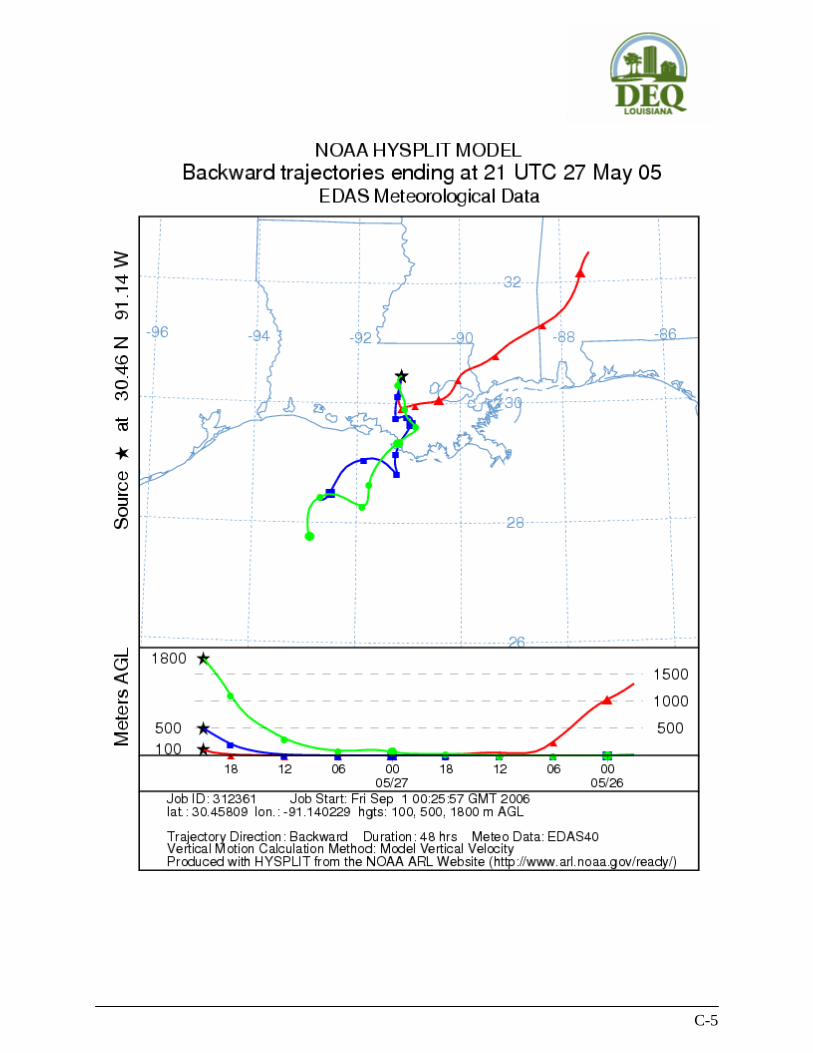
C-5

C-6

C-7

May 19-30, 2003

C-8

C-9

C-10

C-11

September 28-30, 2004

C-12

C-13

April 12-30, 2003

C-14

C-15

C-16

C-17

C-18

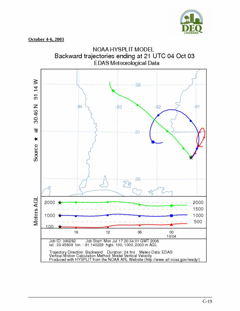
C-19

October 4-6, 2003

C-20

C-21

May 4-9, 2004

C-22

C-23

C-24

C-25

August 11 – September 5, 2000

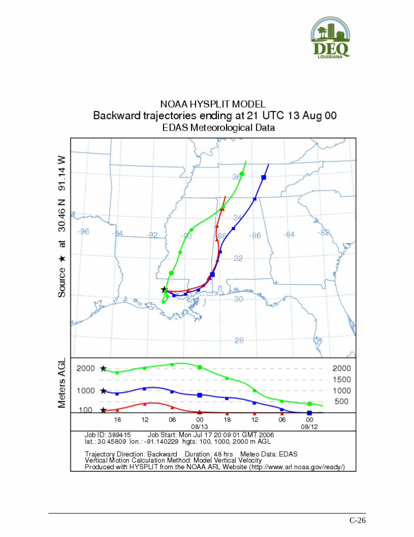
C-26

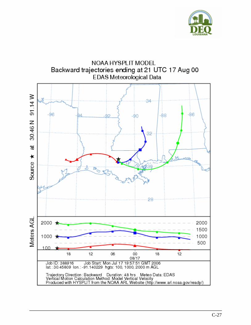
C-27

C-28

C-29

C-30

C-31

C-32

C-33

C-34

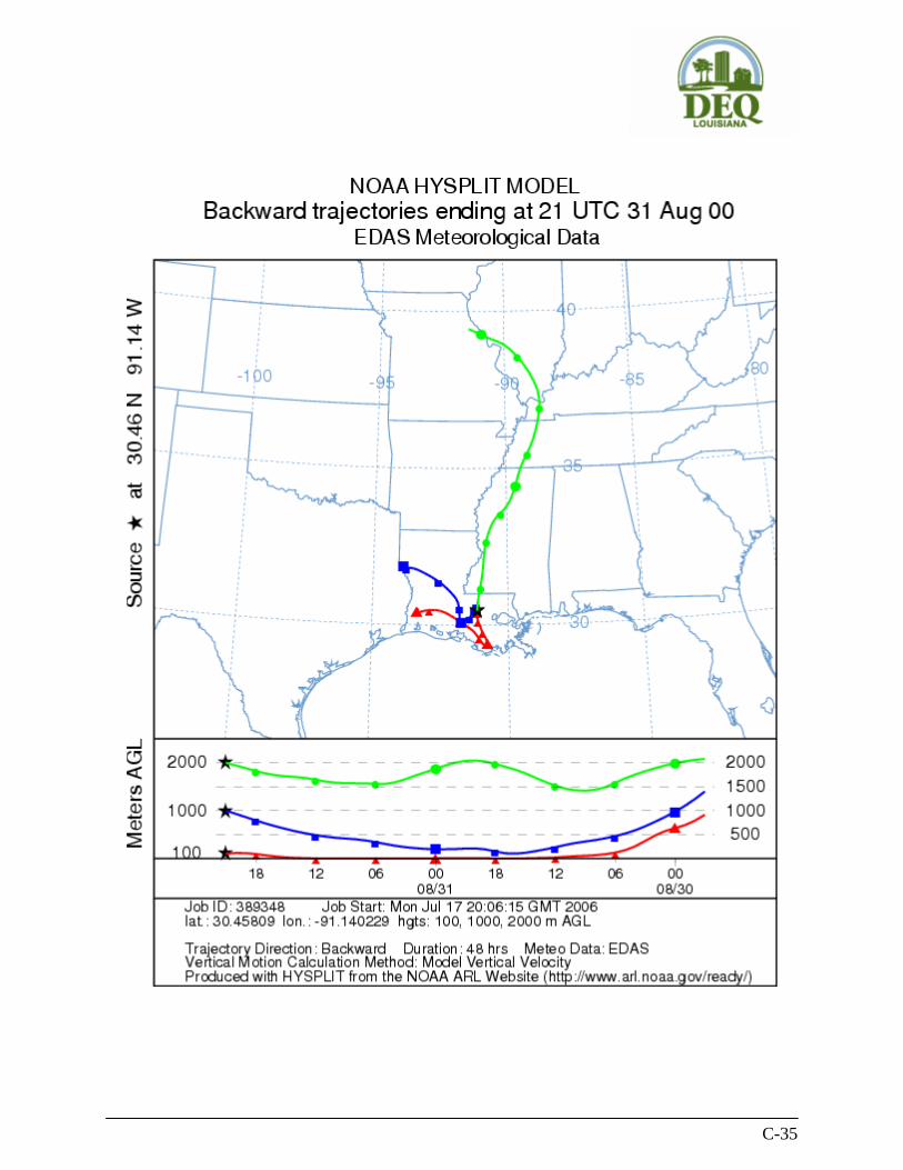
C-35

C-36

C-37

C-38