draft version april 12, 2019 a twocolumn style in aastex62

Draft version April 12, 2019Typeset using LATEX twocolumn style in AASTeX62

Constraining Dark Energy With Stacked Concave Lenses

Fuyu Dong,1 Jun Zhang*,1 Yu Yu,1 Xiaohu Yang,1, 2 HeKun Li,1 Jiaxin Han,1, 3 Wentao Luo,1 Jiajun Zhang,1

and Liping Fu4

1Department of Astronomy, School of Physics and Astronomy, and Shanghai Key Laboratory for Particle Physics and Cosmology,Shanghai Jiao Tong University, Shanghai 200240, China

2IFSA Collaborative Innovation Center, and Tsung-Dao Lee Institute, Shanghai Jiao Tong University, Shanghai 200240, China3Kavli IPMU (WPI), UTIAS, The University of Tokyo, Kashiwa, Chiba 277-8583, Japan

4The Shanghai Key Lab for Astrophysics, Shanghai Normal University, Shanghai 200234, China

ABSTRACT

Low density regions are less affected by the nonlinear structure formation and baryonic physics.

They are ideal places for probing the nature of dark energy, a possible explanation for the cosmic

acceleration. Unlike void lensing, which requires identifications of individual voids, we study the

stacked lensing signals around the low-density-positions (LDP), defined as places that are devoid of

foreground bright galaxies in projection. The method allows a direct comparison with numerical results

by drawing correspondence between the bright galaxies with halos. It leads to lensing signals that are

significant enough for differentiating several dark energy models. In this work, we use the CFHTLenS

catalogue to define LDPs, as well as measuring their background lensing signals. We consider several

different definitions of the foreground bright galaxies (redshift range & magnitude cut). Regarding

the cosmological model, we run six simulations: the first set of simulations have the same initial

conditions, with wde = −1,−0.5,−0.8,−1.2; the second set of simulations include a slightly different

ΛCDM model and a w(z) model from Zhao et al. (2017). The lensing results indicate that the models

with wde = −0.5,−0.8 are not favored, and the other four models all achieve comparable agreement

with the data.

Keywords: Gravitational lensing: weak - Cosmology: large-scale structure of universe - Cosmology:

dark energy - Galaxies: halos

1. INTRODUCTION

The acceleration of the cosmic expansion remains to

be a mystery today (Riess et al. 1998; Perlmutter et al.

1999; Weinberg et al. 2013; Komatsu et al. 2014; Planck

Collaboration et al. 2014). It is not yet clear if it is

necessary to go beyond the simplest ΛCDM model by

introducing a nontrivial equation of state w(z) for dark

energy (Huterer & Turner 1999). Recently, from the

baryon acoustic oscillation measurement of the BOSS

data, there has been intriguing evidence showing a devi-

ation of w(z) from −1 (Zhao et al. 2017). It is desirable

to test the nature of dark energy with alternative cos-

mological probes. We propose to do so with the weak

lensing effect around low density regions.

Low density regions have the advantages of being

much less affected by nonlinear evolution and baryonic

*[email protected]

physics. They are likely the ideal places to test dark en-

ergy models with weak lensing. Previous efforts largely

focus on the lensing effect of voids, a typical type of lowdensity region that is devoid of matter over a significant

cosmic volume.

A major challenge of void lensing is about identifying

the voids. Current void-finding algorithms are mostly

based on the distribution of galaxies with spectroscopic

redshifts. Sanchez et al. (2017) has summarized these

algorithms into several groups: Watershed Void Finders

(Platen et al. 2007; Neyrinck 2008; Lavaux & Wandelt

2012; Nadathur et al. 2015), growth of spherical under-

densities (Hoyle & Vogeley 2002; Colberg et al. 2005;

Padilla et al. 2005; Ceccarelli et al. 2006; Li 2011), hy-

brid methods (Jennings et al. 2013), dynamical criteria

(Elyiv et al. 2015), and Delaunay Triangulation (Zhao

et al. 2016). There are however three main shortcomings

in traditional ways of doing void lensing: 1. void centers

cannot be unambiguously identified due to their intrin-

arX

iv:1

809.

0028

2v3

[as

tro-

ph.C

O]

11

Apr

201

9

mailto: *[email protected]

2 Dong et al.

sically irregular shapes, making it difficult to precisely

predict or understand the stacked void lensing signals

with a physical model; 2. spectroscopic galaxy surveys

are generally expensive, and suffer from complicated in-

fluences from the selection effects; 3. due to the limited

number density of voids and the scatter of their sizes,

the stacked lensing signals do not yet have a high signif-

icance.

More recently, there is a trend to study the lensing

effect of low density regions defined by the projected

galaxy distributions (Clampitt & Jain 2015; Sanchez

et al. 2017; Gruen et al. 2016; Friedrich et al. 2018;

Gruen et al. 2018; Barreira et al. 2017; Davies et al.

2018; Brouwer et al. 2018). Comparing to void lensing,

these new methods only need photo-z information, and

the stacked lensing signals generally have much higher

significance. For example, Gruen et al. (2016) use a

photometrically selected luminous red galaxy sample

(redMaGiC) as the foreground galaxies in their paper.

By dividing the sky into cells, they assign each cell a

weighted and smoothed galaxy count. They do shear

measurements around cells with different galaxy counts

using DES lensing catalogue. Their follow-up works can

be found in Gruen et al. (2018); Friedrich et al. (2018),

in which a complete cosmological analysis is presented

within the LCDM models.

Our approach has similarities to their method, but

also with differences. We consider these low density po-

sitions (“LDPs”), which is defined by excluding the fore-

ground bright galaxies from the sky with a critical radius

in projection. This is a direct way to define the low den-

sity regions, without defining the galaxy density map.

These positions can be similarly defined in N-body sim-

ulations by drawing correspondence between the fore-

ground bright galaxies and halos/subhalos through, e.g.,

subhalo abundance matching (SHAM, e.g., Vale & Os-

triker 2004). These operations are straightforward to

realize, and enable us to directly compare the stacked

lensing signals around LDPs with the simulation pre-

dictions. The motivation of this paper is to differentiate

several different dark energy models through this type

of comparison.

This paper is organized as follows: In §2, we introduce

the basic theory of weak lensing, and the method for

stacking the lensing signals from low density regions in

both observations and numerical simulations; §3 shows

our main results for several different dark energy models;

§4 gives our conclusion and discussions about related

issues.

2. METHOD

2.1. Overview

Figure 1. Source distribution in W1 from CFHTLenScatalogue with apparent magnitude magi < 25.5. The emptyareas in this map are masked out for bright stars.

The background tangential shear is related to the

stacked excess surface density of the foreground (see,

e.g., Peacock (1999)):

∆Σ(R) ≡ Σcr(zl, zs)〈γt〉(R) = Σ(< R)− Σ(R), (1)

where R is the distance to the center, and Σcr(zl, zs) is

the critical surface density in comoving unit, which is

defined as:

Σcr(zl, zs) =c2

4πG

DA(zs)

DA(zl)DA(zl, zs)(1 + zl)2, (2)

where zs and zl are the redshifts of the source and the

lens respectively (zl < zs). Σ(< R) is the meaning sur-

face density within R, and Σ(R) is the surface density

at R. DA refers to the angular diameter distance. By

stacking the background shear signals, Eq.(2) allows us

to probe the average surface density profile around the

foreground objects (e.g., galaxies, cluster centers, void

centers, etc.) directly, with an enhanced significance and

better circular symmetry.

There are in principle no restrictions on how one de-

fines the foreground positions as long as they are physi-

cally meaningful. For our purpose of studying the prop-

erties of dark energy, we consider stacking the shear sig-

nals around LDPs, which are simply defined as places

that are away from foreground bright galaxies (within

a certain narrow redshift range) by more than a critical

distance in projection. LDPs defined in such a way gen-

erally point to low-density regions. They provide abun-

dant foreground positions for shear-stacking, leading to

highly significant lensing signals, as shown in the rest of

the paper.

Constraining Dark Energy With Stacked Concave Lenses 3

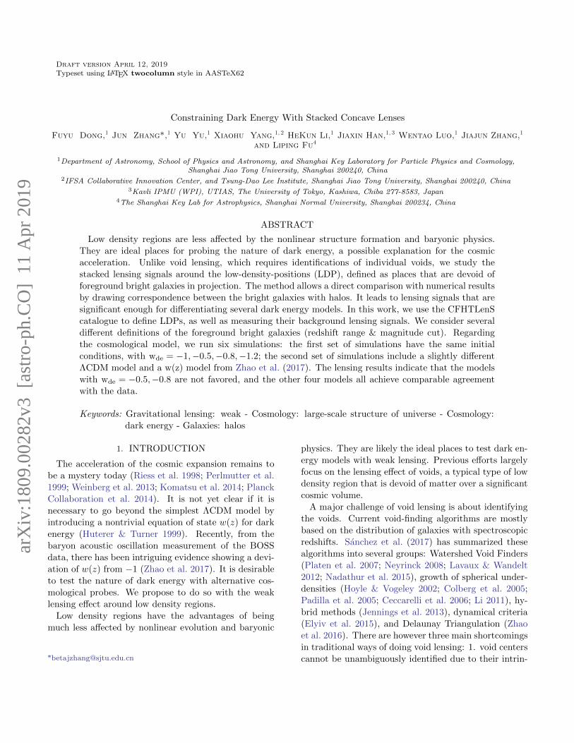
Figure 2. The panel shows galaxy distribution in W1 withabsolute magnitude Magi < −21.5, 0.335 < z < 0.535.

2.2. Observational Data

We use the shear catalogue from CFHTLenS (Canada-

France-Hawaii Telescope Lensing Survey)1, which com-

prises 171 pointings with an effective survey area of

about 154 deg2. The CFHTLenS data set is based on

the Wide part of CFHTLS carried out in four patches:

W1,W2,W3,W4. It has deep photometry in five broad

bands u∗g′r′i′z′ (also the y′ band as a supplement

to i′ band) and limiting magnitude in the i′ band

of i′AB ∼ 25.5. Heymans et al. (2012) presents the

CFHTLenS data analysis pipeline, which summarizes

the weak lensing data processing with THELI (Erben

et al. 2013), shear measurement with Lensfit (Miller

et al. 2013), and photometric redshift measurement with

the Bayesian photometric redshift code (Hildebrandt

et al. 2012).

For each galaxy in the shear catalogue, we are pro-

vided with an inverse-variance weight w, the shape mea-

surement ε1,2, the shear correction terms from calibra-

tion, the apparent and absolute magnitudes (including

extinctions and Magnitude error) in five band, the prob-

ability distribution function (PDF) of redshift, as well

as the peak zp of the PDF. The stacked shears are cal-

culated as (Miller et al. 2013):

γ1,2 =

∑i wi(εi(1,2) − ci(1,2))∑

i wi(1 + mi), (3)

where mi and ci are the multiplicative and additive cal-

ibration terms respectively.

1 http://cfhtlens.org

In order to generate the positions of the LDPs, we use

the foreground bright galaxies above a certain absolute

magnitude, so that the galaxy sample is complete in the

unmasked areas. This allows us to draw correspondence

between the observed galaxies and the halos in simula-

tions, and to construct the average excess surface density

profile around the LDPs in both cases for comparison.

For example, Fig.1 shows the source distribution in W1

from CFHTLenS catalogue with i’ band apparent mag-

nitude less than 25.5 in the W1 area. The differences in

number densities across different fields is quite obvious.

The empty areas in this map are masked out for bright

stars. If only the bright galaxies are kept, the sample be-

comes statistically homogeneous in the unmasked areas

for redshifts that we are interested in. As an example, we

show the distribution of galaxies with 0.335 < z < 0.535

and i’-band absolute magnitude Magi ≤ −21.5 in Fig.2.

The positions of the LDPs are identified through the

following procedures:

1. Generating the LDP candidates

First of all, we require each foreground galaxy to be

brighter than a critical absolute magnitude Magc in the

i′-band, with redshift between [zm-0.1, zm+0.1], where

zm is the median redshift. We circle around each fore-

ground galaxy with radius Rs. Regions within the radius

are removed, and the remaining positions are the can-

didates for LDPs. In principle, there are infinite LDPs.

In this work, for simplicity, we put the LDPs on a uni-

form grid, with the grid size equal to 0.37 arcmin. The

thickness of the redshift slice is set to 0.2 considering

the typical redshift dispersion σz2. Rs

3 here is set to 1

or 1.5 arcmin in order to generate enough LDPs. The

Magc here refers to the critical magnitude in one particu-

lar LCDM model (CW1 in §2.3). For other cosmologies,

we use almost the same foreground galaxy sample4. To

ensure a clean and complete foreground galaxy sample

for generating LDPs, we make three constraints here:

2 We fit each galaxy redshift PDF with a gaussian form to gainthe redshift dispersion σz, which is typically around ∼0.1.

3 There are no restrictions on the way to remove galaxies, and alot of tricks can be done in this process. For example, each galaxycan be assigned with an individual Rs, according to its luminosityor mass. It is also a reasonable way to fix Rs for all the galaxies,as done here.

4 We always select the same amount of brightest galaxies asthe foreground galaxies. For different cosmologies, the rank of thegalaxy brightness may change. For example, for a given apparentmagnitude at redshift z1 and z2, it is possible that the absolutemagnitude Mag(z1,wde1) > Mag(z2,wde1) but Mag(z1,wde2) <Mag(z2,wde2), due to the change of the distance-redshift relation.However, this rarely happens for cosmologies we use.

http://cfhtlens.org

4 Dong et al.

a) We only use sources with star flag = 0 to de-

crease the star contaminations(but not vanished). Over-

all, the fraction of sources with star flag = 1 is around

3%. The ratio becomes ∼ 20% for galaxies satisfying

0.335 < z < 0.535 and Magi < −21. In general, the ra-

tio changes with magnitude and redshift.

b) Galaxies which have two or more close height peaks

in redshift PDF are removed to reduce the redshift un-

certainty. Most of these sources are actually stars. It

further remove ∼ 3% sources for galaxies under condi-

tion star flag = 0, Magi <-21, 0.335 < z < 0.535. This

ratio changes with magnitude and zm.

c) We also remove galaxies with absolute magnitude

Magi <-99 in the original catalogues, which indicates

problems in the measurement. This corresponds to the

removal of 10 percent additional sources. In §4, we show

that these sources generally yield low galaxy-galaxy lens-

ing signals, therefore should not be the foreground galax-

ies we consider.

After the above selection of galaxies, our i-band lumi-

nosity function is consistent with the CFHTLS-DEEP-

SURVEY luminosity function derived by Ramos et al.

(2011).

2. Generating the mask maps

We use the CFHTLenS Mosaic mask files(Erben et al.

2013) in this step. In order to produce the mask maps

in (ra, dec) units, we generate the uniform grids for W1-

4 firstly. Then we apply VENICE5 with these official

files to accurately mask these positions near the mask

boundaries.

3. Finding out the LDPs from candidates

Some of the candidate LDPs generated in step 1

should be removed if they are close to the masked re-

gions. We require the ratio of the masked area to πR2s

around each candidate LDP to be less than 10 percent.

To get rid of the survey edge effects, we also remove the

LDPs whose distances from the edges of the survey area

are less than Rs.

For LDPs generated through steps 1 to 3, we mea-

sure their stacked excess surface density ∆Σ(R) using

background galaxies, and compare it with predictions

of different cosmological simulations introduced in the

next section.

2.3. Simulation

5 https://github.com/jcoupon/venice

Table 1. Simulation parameters.

Simulation wde σ8 Ωc Ωb h ns

CW1 -1 0.85 0.223 0.045 0.71 1

CW2 -0.5 (0.633) 0.223 0.045 0.71 1

CW3 -0.8 (0.789) 0.223 0.045 0.71 1

CW4 -1.2 (0.893) 0.223 0.045 0.71 1

Simulation wde As Ωc Ωb h ns

WZ1 -1 2.2e-9 0.2568 0.0485 0.679 0.968

WZ2 w(z) 2.2e-9 0.24188 0.04525 0.702 0.966

We run two sets of simulations named as CW (stand-

ing for constant w) and WZ (referring to w as a function

of z), the parameters of which are given in table 1. In

all of our simulations, we set Ωde + Ωc + Ωb = 1. 2LPT

and Gadget2 are used to create initial conditions and

run the simulations (Springel & Hernquist 2002; Springel

2005). Both CW and WZ simulations are run from ini-

tial redshift 72 with particle number 10243 and boxsize

600 Mpc/h. We use the FoF group finder to find out the

halos, and the subhalo finder HBT (Han et al. 2012) to

find the subhalos.

i) For CW1, we produce the initial condition following

parameters (σ8 = 0.85,Ωc = 0.223, Ωb = 0.045,ns = 1).

For CW2,3,4 the same initial conditions are used, with

updated H(z) for different wde model in Gadget2. The

value of σ8 in the 4 simulations reduces with increasing

w.

ii) For the second set, we adopt the best fit cosmo-

logical parameters from Zhao et al. (2017) for ΛCDM

and dynamical dark energy w(z) model, and use CAMB

(Lewis et al. 2000) to generate the initial power spec-

trum for the simulation.

The LDPs in simulations are defined in the following

way:

1. Connecting halos/subhalos with galaxies through SHAM

There are different methods in literature to populate

galaxies in dark matter halos/subbhalos: either through

the halo occupation distribution and conditional lumi-

nosity function models (Jing et al. 1998; Berlind & Wein-

berg 2002; Yang et al. 2003; Zheng et al. 2005; van den

Bosch et al. 2007; Zehavi et al. 2011; Leauthaud et al.

2011; Yang et al. 2012; Rodrıguez-Puebla et al. 2015; Zu

& Mandelbaum 2016; Guo et al. 2016; Rodrıguez-Puebla

et al. 2017; Guo et al. 2018), or via subhalo abundance

matching processes (e.g. Vale & Ostriker 2004; Conroy

et al. 2006; Vale & Ostriker 2006; Conroy et al. 2009;

Behroozi et al. 2010; Guo et al. 2010; Simha et al. 2012;

Hearin et al. 2013; Guo & White 2014; Chaves-Montero

et al. 2016; Wechsler & Tinker 2018; Yang et al. 2018).

https://github.com/jcoupon/venice


Figure 3. The figure shows galaxy distributionfrom one sub-area of CW1 simulation for Magi <-21.5,0.335 < z < 0.535.

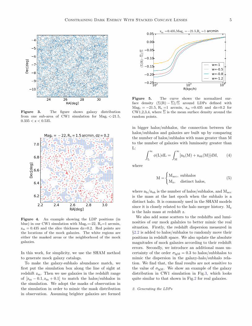
Figure 4. An example showing the LDP positions (inblue) in our CW1 simulation with Magc=-22, Rs=1 arcmin,zm = 0.435 and the slice thickness dz=0.2. Red points arethe locations of the mock galaxies. The white regions areeither the masked areas or the neighborhood of the mockgalaxies.

In this work, for simplicity, we use the SHAM method

to generate mock galaxy catalogs.

To make the galaxy-subhalo abundance match, we

first put the simulation box along the line of sight at

redshift zm. Then we use galaxies in the redshift range

of [zm − 0.1, zm + 0.1] to match the halos/subhalos in

the simulation. We adopt the masks of observation in

the simulation in order to mimic the mask distribution

in observation. Assuming brighter galaxies are formed

102 103 104

R(kpc/h)

0.25

0.20

0.15

0.10

0.05

0.00

0.05

(Σ(R

)−Σ

)/Σ

zm =0.435,Magc =−21.5,Rs =1 arcmin

w=-1

w=-0.5

w=-0.8

w=-1.2

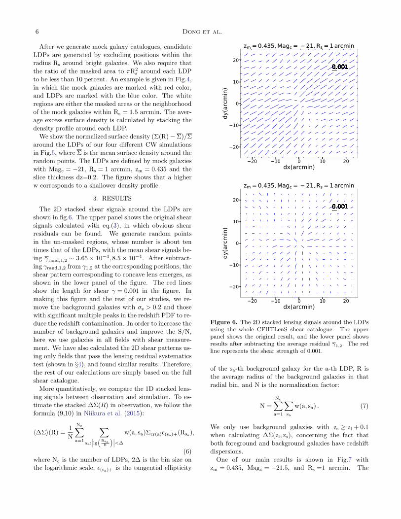
Figure 5. The curve shows the normalized sur-face density (Σ(R)− Σ)/Σ around LDPs defined withMagc = −21.5, Rs =1 arcmin, zm =0.435 and dz=0.2 forCW1,2,3,4, where Σ is the mean surface density around therandom points.

in bigger halos/subhalos, the connection between the

halos/subhalos and galaxies are built up by comparing

the number of halos/subhalos with mass greater than M

to the number of galaxies with luminosity greater than

L: ∫ ∞L

φ(L)dL =

∫ ∞M

[nh(M) + nsh(M)]dM, (4)

where

M =

Macc, subhalos

Mz, distinct halos,(5)

where nh/nsh is the number of halos/subhalos, and Macc

is the mass at the last epoch when the subhalo is a

distinct halo. It is commonly used in the SHAM models

since it is closely related to the halo merger history. Mz

is the halo mass at redshift z.

We also add some scatters to the redshifts and lumi-

nosities of our mock galalxies to better mimic the real

situation. Firstly, the redshift dispersion measured in

§2.2 is added to halos/subhalos to randomly move their

positions in redshift space. We also update the absolute

magnitudes of mock galaxies according to their redshift

errors. Secondly, we introduce an additional mass un-

certainty of the order σlgM = 0.3 to halos/subbhalos to

mimic the dispersion in the galaxy-halo/subhalo rela-

tion. We find that, the final results are not sensitive to

the value of σlgM. We show an example of the galaxy

distribution in CW1 simulation in Fig.3, which looks

quite similar to that shown in Fig.2 for real galaxies.

2. Generating the LDPs

6 Dong et al.

After we generate mock galaxy catalogues, candidate

LDPs are generated by excluding positions within the

radius Rs around bright galaxies. We also require that

the ratio of the masked area to πR2s around each LDP

to be less than 10 percent. An example is given in Fig.4,

in which the mock galaxies are marked with red color,

and LDPs are marked with the blue color. The white

regions are either the masked areas or the neighborhood

of the mock galaxies within Rs = 1.5 arcmin. The aver-

age excess surface density is calculated by stacking the

density profile around each LDP.

We show the normalized surface density (Σ(R)− Σ)/Σ

around the LDPs of our four different CW simulations

in Fig.5, where Σ is the mean surface density around the

random points. The LDPs are defined by mock galaxies

with Magc = −21, Rs = 1 arcmin, zm = 0.435 and the

slice thickness dz=0.2. The figure shows that a higher

w corresponds to a shallower density profile.

3. RESULTS

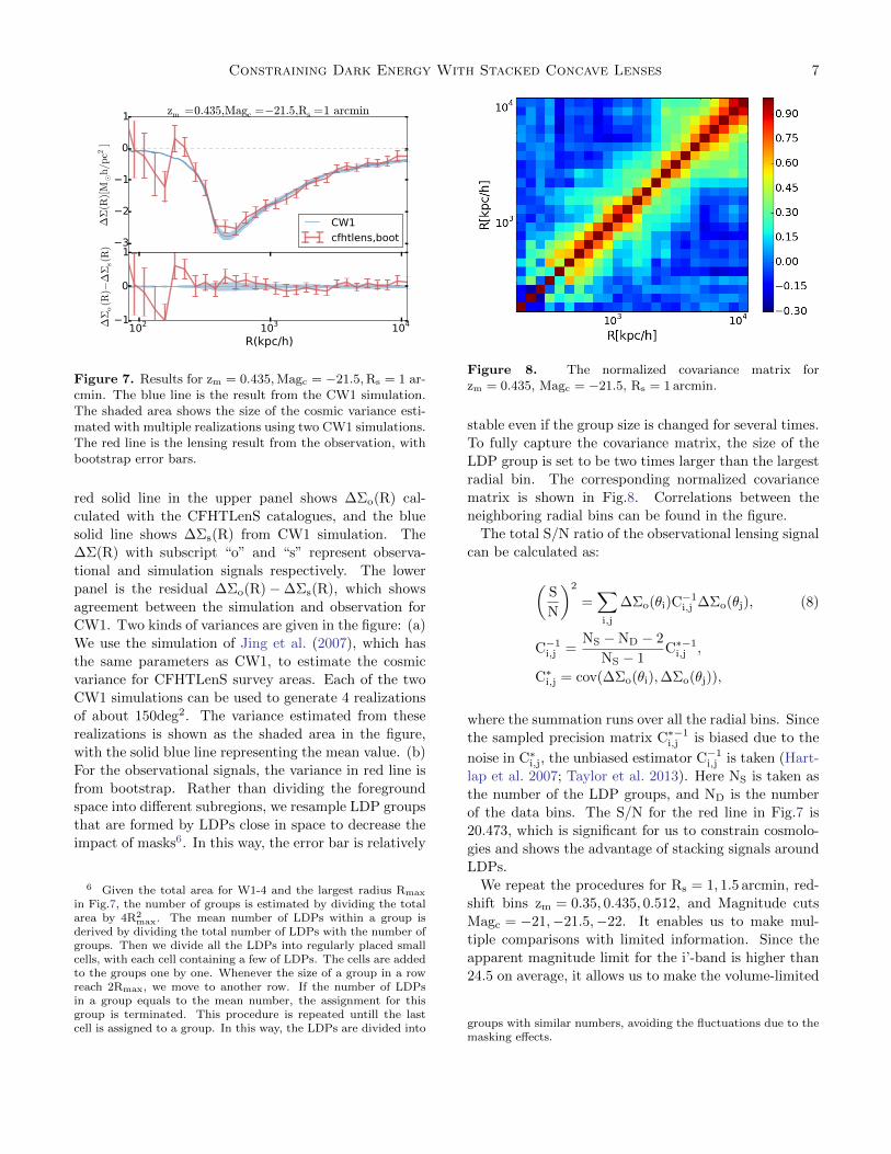
The 2D stacked shear signals around the LDPs are

shown in fig.6. The upper panel shows the original shear

signals calculated with eq.(3), in which obvious shear

residuals can be found. We generate random points

in the un-masked regions, whose number is about ten

times that of the LDPs, with the mean shear signals be-

ing γrand,1,2 ∼ 3.65× 10−4, 8.5× 10−4. After subtract-

ing γrand,1,2 from γ1,2 at the corresponding positions, the

shear pattern corresponding to concave lens emerges, as

shown in the lower panel of the figure. The red lines

show the length for shear γ = 0.001 in the figure. In

making this figure and the rest of our studies, we re-

move the background galaxies with σz > 0.2 and those

with significant multiple peaks in the redshift PDF to re-

duce the redshift contamination. In order to increase the

number of background galaxies and improve the S/N,

here we use galaxies in all fields with shear measure-

ment. We have also calculated the 2D shear patterns us-

ing only fields that pass the lensing residual systematics

test (shown in §4), and found similar results. Therefore,

the rest of our calculations are simply based on the full

shear catalogue.

More quantitatively, we compare the 1D stacked lens-

ing signals between observation and simulation. To es-

timate the stacked ∆Σ(R) in observation, we follow the

formula (9,10) in Niikura et al. (2015):

〈∆Σ〉(R) =1

N

Nc∑a=1

∑sa:

∣∣∣lg(RsaR

)∣∣∣<∆

w(a, sa)Σcr(a)ε(sa)+(Rsa),

(6)

where Nc is the number of LDPs, 2∆ is the bin size on

the logarithmic scale, ε(sa)+ is the tangential ellipticity

20 10 0 10 20dx(arcmin)

20

10

0

10

20

dy(a

rcm

in)

0.0010.0010.0010.0010.0010.0010.0010.0010.0010.0010.0010.0010.0010.0010.0010.0010.0010.0010.0010.0010.0010.0010.0010.0010.0010.0010.0010.0010.0010.0010.0010.0010.0010.0010.0010.0010.0010.0010.0010.0010.0010.0010.0010.0010.0010.0010.0010.0010.0010.0010.0010.0010.0010.0010.0010.0010.0010.0010.0010.0010.0010.0010.0010.0010.0010.0010.0010.0010.0010.0010.0010.0010.0010.0010.0010.0010.0010.0010.0010.0010.0010.0010.0010.0010.0010.0010.0010.0010.0010.0010.0010.0010.0010.0010.0010.0010.0010.0010.0010.0010.0010.0010.0010.0010.0010.0010.0010.0010.0010.0010.0010.0010.0010.0010.0010.0010.0010.0010.0010.0010.0010.0010.0010.0010.0010.0010.0010.0010.0010.0010.0010.0010.0010.0010.0010.0010.0010.0010.0010.0010.0010.0010.0010.0010.0010.0010.0010.0010.0010.0010.0010.0010.0010.0010.0010.0010.0010.0010.0010.0010.0010.0010.0010.0010.0010.0010.0010.0010.0010.0010.0010.0010.0010.0010.0010.0010.0010.0010.0010.0010.0010.0010.0010.0010.0010.0010.0010.0010.0010.0010.0010.0010.0010.0010.0010.0010.0010.0010.0010.0010.0010.0010.0010.0010.0010.0010.0010.0010.0010.0010.0010.0010.0010.0010.0010.0010.0010.0010.0010.0010.0010.0010.0010.0010.0010.0010.0010.0010.0010.0010.0010.0010.0010.0010.0010.0010.0010.0010.0010.0010.0010.0010.0010.0010.0010.0010.0010.0010.0010.0010.0010.0010.0010.0010.0010.0010.0010.0010.0010.0010.0010.0010.0010.0010.0010.0010.0010.0010.0010.0010.0010.0010.0010.0010.0010.0010.0010.0010.0010.0010.0010.0010.0010.0010.0010.0010.0010.0010.0010.0010.0010.0010.0010.0010.0010.0010.0010.0010.0010.0010.0010.0010.0010.0010.0010.0010.0010.0010.0010.0010.0010.0010.0010.0010.0010.0010.0010.0010.0010.0010.0010.0010.0010.0010.0010.0010.0010.0010.0010.0010.0010.0010.0010.0010.0010.0010.0010.0010.0010.0010.0010.0010.0010.0010.0010.0010.0010.0010.0010.0010.0010.0010.0010.0010.0010.0010.0010.0010.0010.0010.0010.0010.0010.0010.0010.0010.0010.0010.0010.0010.0010.0010.0010.0010.0010.0010.0010.0010.0010.0010.0010.0010.0010.0010.0010.0010.0010.0010.0010.0010.0010.0010.0010.0010.0010.0010.0010.0010.0010.001

zm = 0.435, Magc = 21, Rs = 1 arcmin

20 10 0 10 20dx(arcmin)

20

10

0

10

20

dy(a

rcm

in)

0.0010.0010.0010.0010.0010.0010.0010.0010.0010.0010.0010.0010.0010.0010.0010.0010.0010.0010.0010.0010.0010.0010.0010.0010.0010.0010.0010.0010.0010.0010.0010.0010.0010.0010.0010.0010.0010.0010.0010.0010.0010.0010.0010.0010.0010.0010.0010.0010.0010.0010.0010.0010.0010.0010.0010.0010.0010.0010.0010.0010.0010.0010.0010.0010.0010.0010.0010.0010.0010.0010.0010.0010.0010.0010.0010.0010.0010.0010.0010.0010.0010.0010.0010.0010.0010.0010.0010.0010.0010.0010.0010.0010.0010.0010.0010.0010.0010.0010.0010.0010.0010.0010.0010.0010.0010.0010.0010.0010.0010.0010.0010.0010.0010.0010.0010.0010.0010.0010.0010.0010.0010.0010.0010.0010.0010.0010.0010.0010.0010.0010.0010.0010.0010.0010.0010.0010.0010.0010.0010.0010.0010.0010.0010.0010.0010.0010.0010.0010.0010.0010.0010.0010.0010.0010.0010.0010.0010.0010.0010.0010.0010.0010.0010.0010.0010.0010.0010.0010.0010.0010.0010.0010.0010.0010.0010.0010.0010.0010.0010.0010.0010.0010.0010.0010.0010.0010.0010.0010.0010.0010.0010.0010.0010.0010.0010.0010.0010.0010.0010.0010.0010.0010.0010.0010.0010.0010.0010.0010.0010.0010.0010.0010.0010.0010.0010.0010.0010.0010.0010.0010.0010.0010.0010.0010.0010.0010.0010.0010.0010.0010.0010.0010.0010.0010.0010.0010.0010.0010.0010.0010.0010.0010.0010.0010.0010.0010.0010.0010.0010.0010.0010.0010.0010.0010.0010.0010.0010.0010.0010.0010.0010.0010.0010.0010.0010.0010.0010.0010.0010.0010.0010.0010.0010.0010.0010.0010.0010.0010.0010.0010.0010.0010.0010.0010.0010.0010.0010.0010.0010.0010.0010.0010.0010.0010.0010.0010.0010.0010.0010.0010.0010.0010.0010.0010.0010.0010.0010.0010.0010.0010.0010.0010.0010.0010.0010.0010.0010.0010.0010.0010.0010.0010.0010.0010.0010.0010.0010.0010.0010.0010.0010.0010.0010.0010.0010.0010.0010.0010.0010.0010.0010.0010.0010.0010.0010.0010.0010.0010.0010.0010.0010.0010.0010.0010.0010.0010.0010.0010.0010.0010.0010.0010.0010.0010.0010.0010.0010.0010.0010.0010.0010.0010.0010.0010.0010.0010.0010.0010.0010.0010.0010.0010.0010.0010.0010.0010.0010.0010.0010.0010.0010.0010.0010.0010.0010.0010.0010.0010.0010.001

zm = 0.435, Magc = 21, Rs = 1 arcmin

Figure 6. The 2D stacked lensing signals around the LDPsusing the whole CFHTLenS shear catalogue. The upperpanel shows the original result, and the lower panel showsresults after subtracting the average residual γ1,2. The redline represents the shear strength of 0.001.

of the sa-th background galaxy for the a-th LDP, R is

the average radius of the background galaxies in that

radial bin, and N is the normalization factor:

N =

Nc∑a=1

∑sa

w(a, sa) . (7)

We only use background galaxies with zs ≥ zl + 0.1

when calculating ∆Σ(zl, zs), concerning the fact that

both foreground and background galaxies have redshift

dispersions.

One of our main results is shown in Fig.7 with

zm = 0.435, Magc = −21.5, and Rs =1 arcmin. The


R(kpc/h)

1

0

1

2

3

∆Σ

(R)[M

¯h/p

c2]

zm =0.435,Magc =−21.5,Rs =1 arcmin

CW1

cfhtlens,boot

102 103 104

R(kpc/h)

1

0

1∆Σ

o(R

)−∆

Σs(R

)

Figure 7. Results for zm = 0.435,Magc = −21.5,Rs = 1 ar-cmin. The blue line is the result from the CW1 simulation.The shaded area shows the size of the cosmic variance esti-mated with multiple realizations using two CW1 simulations.The red line is the lensing result from the observation, withbootstrap error bars.

red solid line in the upper panel shows ∆Σo(R) cal-

culated with the CFHTLenS catalogues, and the blue

solid line shows ∆Σs(R) from CW1 simulation. The

∆Σ(R) with subscript “o” and “s” represent observa-

tional and simulation signals respectively. The lower

panel is the residual ∆Σo(R)−∆Σs(R), which shows

agreement between the simulation and observation for

CW1. Two kinds of variances are given in the figure: (a)

We use the simulation of Jing et al. (2007), which has

the same parameters as CW1, to estimate the cosmic

variance for CFHTLenS survey areas. Each of the two

CW1 simulations can be used to generate 4 realizations

of about 150deg2. The variance estimated from these

realizations is shown as the shaded area in the figure,

with the solid blue line representing the mean value. (b)

For the observational signals, the variance in red line is

from bootstrap. Rather than dividing the foreground

space into different subregions, we resample LDP groups

that are formed by LDPs close in space to decrease the

impact of masks6. In this way, the error bar is relatively

6 Given the total area for W1-4 and the largest radius Rmax

in Fig.7, the number of groups is estimated by dividing the totalarea by 4R2

max. The mean number of LDPs within a group isderived by dividing the total number of LDPs with the number ofgroups. Then we divide all the LDPs into regularly placed smallcells, with each cell containing a few of LDPs. The cells are addedto the groups one by one. Whenever the size of a group in a rowreach 2Rmax, we move to another row. If the number of LDPsin a group equals to the mean number, the assignment for thisgroup is terminated. This procedure is repeated untill the lastcell is assigned to a group. In this way, the LDPs are divided into

Figure 8. The normalized covariance matrix forzm = 0.435, Magc = −21.5, Rs = 1 arcmin.

stable even if the group size is changed for several times.

To fully capture the covariance matrix, the size of the

LDP group is set to be two times larger than the largest

radial bin. The corresponding normalized covariance

matrix is shown in Fig.8. Correlations between the

neighboring radial bins can be found in the figure.

The total S/N ratio of the observational lensing signal

can be calculated as:

(S

N

)2

=∑i,j

∆Σo(θi)C−1i,j ∆Σo(θj), (8)

C−1i,j =

NS −ND − 2

NS − 1C∗−1

i,j ,

C∗i,j = cov(∆Σo(θi),∆Σo(θj)),

where the summation runs over all the radial bins. Since

the sampled precision matrix C∗−1i,j is biased due to the

noise in C∗i,j, the unbiased estimator C−1i,j is taken (Hart-

lap et al. 2007; Taylor et al. 2013). Here NS is taken as

the number of the LDP groups, and ND is the number

of the data bins. The S/N for the red line in Fig.7 is

20.473, which is significant for us to constrain cosmolo-

gies and shows the advantage of stacking signals around

LDPs.

We repeat the procedures for Rs = 1, 1.5 arcmin, red-

shift bins zm = 0.35, 0.435, 0.512, and Magnitude cuts

Magc = −21,−21.5,−22. It enables us to make mul-

tiple comparisons with limited information. Since the

apparent magnitude limit for the i’-band is higher than

24.5 on average, it allows us to make the volume-limited

groups with similar numbers, avoiding the fluctuations due to themasking effects.

8 Dong et al.

r(kpc/h)

1

0

1

2

3

∆Σ

s(R

)[M

¯h/p

c2]

zm =0.35, Rs =1arcmin, Magc =−21zm =0.35, Rs =1arcmin, Magc =−21zm =0.35, Rs =1arcmin, Magc =−21zm =0.35, Rs =1arcmin, Magc =−21zm =0.35, Rs =1arcmin, Magc =−21zm =0.35, Rs =1arcmin, Magc =−21

102 103 104

R(kpc/h)

1

0

1

∆Σ

o(R

)−∆

Σs(R

)

r(kpc/h)

Magc =−21.5Magc =−21.5Magc =−21.5Magc =−21.5Magc =−21.5Magc =−21.5

102 103 104

R(kpc/h)

r(kpc/h)

Magc =−22Magc =−22Magc =−22Magc =−22Magc =−22Magc =−22

CW1

CW2

CW3

CW4

WZ1

WZ2

102 103 104

R(kpc/h)

r(kpc/h)

1

0

1

2

3

∆Σ

s(R

)[M

¯h/pc2

]


102 103 104

R(kpc/h)

1

0

1

∆Σ

o(R

)−∆

Σs(R

)

r(kpc/h)


102 103 104

R(kpc/h)

r(kpc/h)


CW1

CW2

CW3

CW4

WZ1

WZ2

102 103 104

R(kpc/h)

r(kpc/h)

1

0

1

2

3

∆Σ

s(R

)[M

¯h/p

c2]


102 103 104

R(kpc/h)

1

0

1

∆Σ

o(R

)−∆

Σs(R

)

r(kpc/h)


102 103 104

R(kpc/h)

r(kpc/h)


CW1

CW2

CW3

CW4

WZ1

WZ2

102 103 104

R(kpc/h)

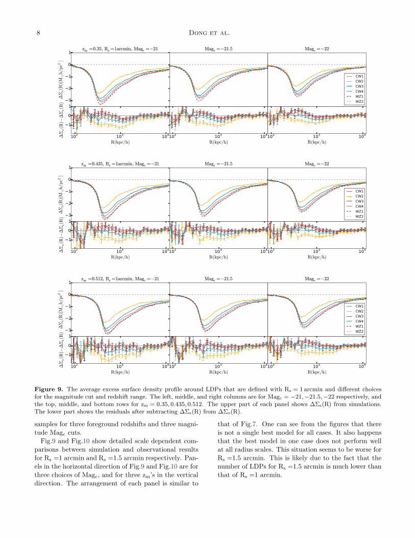
Figure 9. The average excess surface density profile around LDPs that are defined with Rs = 1 arcmin and different choicesfor the magnitude cut and redshift range. The left, middle, and right columns are for Magc = −21,−21.5,−22 respectively, andthe top, middle, and bottom rows for zm = 0.35, 0.435, 0.512. The upper part of each panel shows ∆Σs(R) from simulations.The lower part shows the residuals after subtracting ∆Σs(R) from ∆Σo(R).

samples for three foreground redshifts and three magni-

tude Magc cuts.

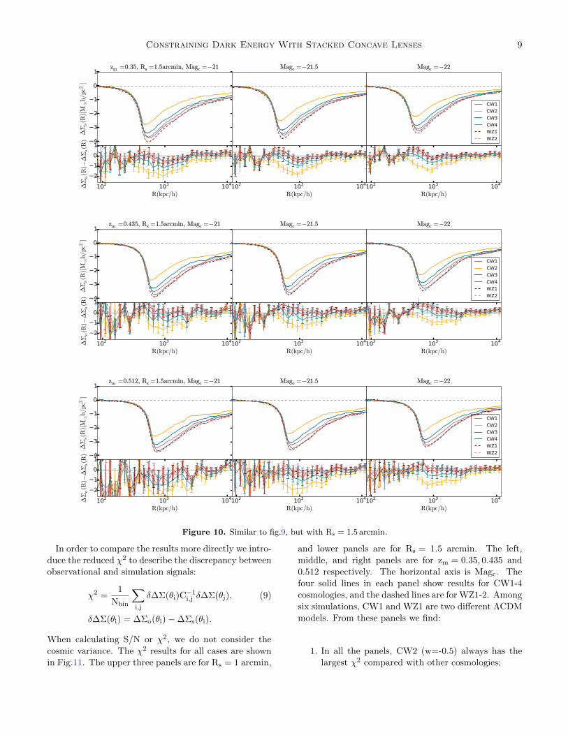
Fig.9 and Fig.10 show detailed scale dependent com-

parisons between simulation and observational results

for Rs =1 arcmin and Rs =1.5 arcmin respectively. Pan-

els in the horizontal direction of Fig.9 and Fig.10 are for

three choices of Magc, and for three zm’s in the vertical

direction. The arrangement of each panel is similar to

that of Fig.7. One can see from the figures that there

is not a single best model for all cases. It also happens

that the best model in one case does not perform well

at all radius scales. This situation seems to be worse for

Rs =1.5 arcmin. This is likely due to the fact that the

number of LDPs for Rs =1.5 arcmin is much lower than

that of Rs =1 arcmin.


r(kpc/h)

1

0

1

2

3

4

∆Σ

s(R

)[M

¯h/p

c2]

zm =0.35, Rs =1.5arcmin, Magc =−21zm =0.35, Rs =1.5arcmin, Magc =−21zm =0.35, Rs =1.5arcmin, Magc =−21zm =0.35, Rs =1.5arcmin, Magc =−21zm =0.35, Rs =1.5arcmin, Magc =−21zm =0.35, Rs =1.5arcmin, Magc =−21

102 103 104

R(kpc/h)

1

0

1

2

∆Σ

o(R

)−∆

Σs(R

)

r(kpc/h)


102 103 104

R(kpc/h)

r(kpc/h)


CW1

CW2

CW3

CW4

WZ1

WZ2

102 103 104

R(kpc/h)

r(kpc/h)

1

0

1

2

3

4

∆Σ

s(R

)[M

¯h/pc2

]


102 103 104

R(kpc/h)

1

0

1

2

∆Σ

o(R

)−∆

Σs(R

)

r(kpc/h)


102 103 104

R(kpc/h)

r(kpc/h)


CW1

CW2

CW3

CW4

WZ1

WZ2

102 103 104

R(kpc/h)

r(kpc/h)

1

0

1

2

3

4

∆Σ

s(R

)[M

¯h/p

c2]


102 103 104

R(kpc/h)

1

0

1

2

∆Σ

o(R

)−∆

Σs(R

)

r(kpc/h)


102 103 104

R(kpc/h)

r(kpc/h)


CW1

CW2

CW3

CW4

WZ1

WZ2

102 103 104

R(kpc/h)

Figure 10. Similar to fig.9, but with Rs = 1.5 arcmin.

In order to compare the results more directly we intro-

duce the reduced χ2 to describe the discrepancy between

observational and simulation signals:

χ2 =1

Nbin

∑i,j

δ∆Σ(θi)C−1i,j δ∆Σ(θj), (9)

δ∆Σ(θi) = ∆Σo(θi)−∆Σs(θi).

When calculating S/N or χ2, we do not consider the

cosmic variance. The χ2 results for all cases are shown

in Fig.11. The upper three panels are for Rs = 1 arcmin,

and lower panels are for Rs = 1.5 arcmin. The left,

middle, and right panels are for zm = 0.35, 0.435 and

0.512 respectively. The horizontal axis is Magc. The

four solid lines in each panel show results for CW1-4

cosmologies, and the dashed lines are for WZ1-2. Among

six simulations, CW1 and WZ1 are two different ΛCDM

models. From these panels we find:

1. In all the panels, CW2 (w=-0.5) always has the

largest χ2 compared with other cosmologies;

10 Dong et al.

-21 -21.5 -220

2

4

6

8

10

122

zm = 0.35, Rs = 1 arcmin

CW1CW2CW3CW4WZ1WZ2

-21 -21.5 -220

2

4

6

8

10

12zm = 0.435, Rs = 1 arcmin

-21 -21.5 -220

2

4

6

8

10

12zm = 0.512, Rs = 1 arcmin

-21 -21.5 -22Magc

0

2

4

6

8

10

12

2

zm = 0.35, Rs = 1.5 arcmin

-21 -21.5 -22Magc

0

1

2

3

4

5

6

7

8zm = 0.435, Rs = 1.5 arcmin

-21 -21.5 -22Magc

0

1

2

3

4

5

6

7

8zm = 0.512, Rs = 1.5 arcmin

Figure 11. The reduced χ2 for six cosmologies with different choices of Magc, Rs and zm. The upper three panels are forRs = 1 arcmin, and lower panels are for Rs = 1.5 arcmin. The left, middle, and right columns are for zm = 0.35, 0.435, 0.512respectively. The horizontal axis in each plot is the magnitude cut Magc.

2. CW3 (w=-0.8) has the second largest χ2 in most

cases;

3. The other four models, including the two ΛCDM

models (CW1,WZ1), the CW4 (w=-1.2) model,

and WZ2 (dynamical w(z)), all have comparably

low χ2 i n most cases. The most pronounced ex-

ception is in the case of zm = 0.435, Rs = 1.5 ar-

cmin, and Magc = −22, in which the CW3 model

yields the lowest χ2 in contrast.

4. CONCLUSION AND DISCUSSIONS

In this paper we study the stacked lensing signals

around the low-density-positions (LDPs), which are de-

fined as places that are devoid of foreground bright

galaxies in projection. We show how to define the fore-

ground galaxy population and locate the LDPs in the

presence of masks using the CFHTLenS data. Different

redshift ranges and magnitude cuts are considered for

the foreground population. The measured excess sur-

101 102 103 104

r[kpc/h]

10-1

100

101

102

103

∆Σ

t(r

)[M

¯h/p

c2]

galaxy-galaxy lensing, zm =0.435

[<-99],Ng=31530

[-21,-21.5],Ng=81259

[-21.5,-22],Ng=68505

[-22,-22.5],Ng=51667

Figure 12. Galaxy-galaxy lensing signals for foregroundgalaxies in the Magnitude bins of [-21,-21.5], [-21.5,-22], [-22,-22.5] and [< − 99], and redshift range of [0.335,0.435].Ng is the number of foreground galaxies.


20 10 0 10 20dx(arcmin)

20

10

0

10

20dy

(arc

min

)0.0010.0010.0010.0010.0010.0010.0010.0010.0010.0010.0010.0010.0010.0010.0010.0010.0010.0010.0010.0010.0010.0010.0010.0010.0010.0010.0010.0010.0010.0010.0010.0010.0010.0010.0010.0010.0010.0010.0010.0010.0010.0010.0010.0010.0010.0010.0010.0010.0010.0010.0010.0010.0010.0010.0010.0010.0010.0010.0010.0010.0010.0010.0010.0010.0010.0010.0010.0010.0010.0010.0010.0010.0010.0010.0010.0010.0010.0010.0010.0010.0010.0010.0010.0010.0010.0010.0010.0010.0010.0010.0010.0010.0010.0010.0010.0010.0010.0010.0010.0010.0010.0010.0010.0010.0010.0010.0010.0010.0010.0010.0010.0010.0010.0010.0010.0010.0010.0010.0010.0010.0010.0010.0010.0010.0010.0010.0010.0010.0010.0010.0010.0010.0010.0010.0010.0010.0010.0010.0010.0010.0010.0010.0010.0010.0010.0010.0010.0010.0010.0010.0010.0010.0010.0010.0010.0010.0010.0010.0010.0010.0010.0010.0010.0010.0010.0010.0010.0010.0010.0010.0010.0010.0010.0010.0010.0010.0010.0010.0010.0010.0010.0010.0010.0010.0010.0010.0010.0010.0010.0010.0010.0010.0010.0010.0010.0010.0010.0010.0010.0010.0010.0010.0010.0010.0010.0010.0010.0010.0010.0010.0010.0010.0010.0010.0010.0010.0010.0010.0010.0010.0010.0010.0010.0010.0010.0010.0010.0010.0010.0010.0010.0010.0010.0010.0010.0010.0010.0010.0010.0010.0010.0010.0010.0010.0010.0010.0010.0010.0010.0010.0010.0010.0010.0010.0010.0010.0010.0010.0010.0010.0010.0010.0010.0010.0010.0010.0010.0010.0010.0010.0010.0010.0010.0010.0010.0010.0010.0010.0010.0010.0010.0010.0010.0010.0010.0010.0010.0010.0010.0010.0010.0010.0010.0010.0010.0010.0010.0010.0010.0010.0010.0010.0010.0010.0010.0010.0010.0010.0010.0010.0010.0010.0010.0010.0010.0010.0010.0010.0010.0010.0010.0010.0010.0010.0010.0010.0010.0010.0010.0010.0010.0010.0010.0010.0010.0010.0010.0010.0010.0010.0010.0010.0010.0010.0010.0010.0010.0010.0010.0010.0010.0010.0010.0010.0010.0010.0010.0010.0010.0010.0010.0010.0010.0010.0010.0010.0010.0010.0010.0010.0010.0010.0010.0010.0010.0010.0010.0010.0010.0010.0010.0010.0010.0010.0010.0010.0010.0010.0010.0010.0010.0010.0010.0010.0010.0010.0010.0010.0010.001

zm = 0.435, Magc = 21, Rs = 1 arcmin

20 10 0 10 20dx(arcmin)

20

10

0

10

20

dy(a

rcm

in)

0.0010.0010.0010.0010.0010.0010.0010.0010.0010.0010.0010.0010.0010.0010.0010.0010.0010.0010.0010.0010.0010.0010.0010.0010.0010.0010.0010.0010.0010.0010.0010.0010.0010.0010.0010.0010.0010.0010.0010.0010.0010.0010.0010.0010.0010.0010.0010.0010.0010.0010.0010.0010.0010.0010.0010.0010.0010.0010.0010.0010.0010.0010.0010.0010.0010.0010.0010.0010.0010.0010.0010.0010.0010.0010.0010.0010.0010.0010.0010.0010.0010.0010.0010.0010.0010.0010.0010.0010.0010.0010.0010.0010.0010.0010.0010.0010.0010.0010.0010.0010.0010.0010.0010.0010.0010.0010.0010.0010.0010.0010.0010.0010.0010.0010.0010.0010.0010.0010.0010.0010.0010.0010.0010.0010.0010.0010.0010.0010.0010.0010.0010.0010.0010.0010.0010.0010.0010.0010.0010.0010.0010.0010.0010.0010.0010.0010.0010.0010.0010.0010.0010.0010.0010.0010.0010.0010.0010.0010.0010.0010.0010.0010.0010.0010.0010.0010.0010.0010.0010.0010.0010.0010.0010.0010.0010.0010.0010.0010.0010.0010.0010.0010.0010.0010.0010.0010.0010.0010.0010.0010.0010.0010.0010.0010.0010.0010.0010.0010.0010.0010.0010.0010.0010.0010.0010.0010.0010.0010.0010.0010.0010.0010.0010.0010.0010.0010.0010.0010.0010.0010.0010.0010.0010.0010.0010.0010.0010.0010.0010.0010.0010.0010.0010.0010.0010.0010.0010.0010.0010.0010.0010.0010.0010.0010.0010.0010.0010.0010.0010.0010.0010.0010.0010.0010.0010.0010.0010.0010.0010.0010.0010.0010.0010.0010.0010.0010.0010.0010.0010.0010.0010.0010.0010.0010.0010.0010.0010.0010.0010.0010.0010.0010.0010.0010.0010.0010.0010.0010.0010.0010.0010.0010.0010.0010.0010.0010.0010.0010.0010.0010.0010.0010.0010.0010.0010.0010.0010.0010.0010.0010.0010.0010.0010.0010.0010.0010.0010.0010.0010.0010.0010.0010.0010.0010.0010.0010.0010.0010.0010.0010.0010.0010.0010.0010.0010.0010.0010.0010.0010.0010.0010.0010.0010.0010.0010.0010.0010.0010.0010.0010.0010.0010.0010.0010.0010.0010.0010.0010.0010.0010.0010.0010.0010.0010.0010.0010.0010.0010.0010.0010.0010.0010.0010.0010.0010.0010.0010.0010.0010.0010.0010.0010.0010.0010.0010.0010.0010.0010.0010.0010.0010.0010.0010.0010.0010.0010.0010.0010.0010.001

zm = 0.435, Magc = 21, Rs = 1 arcmin

Figure 13. The 2D stacked lensing signals around the LDPs using only the CFHTLenS fields that pass the lensing residualsystematics tests. The left panel shows the original result, and the right panel shows results after subtracting the averageresidual γ1,2. The red line represents the shear strength of 0.001.

face density profiles can be compared with the predic-

tions from simulations. The comparison is made avail-

able by drawing correspondence between galaxies and

halos/subhalos via SHAM.

With the CFHTLenS shear catalogue, we have suc-

cessfully measured the lensing signals around the LDPs

with a high significance. These measurements are used

to constrain dark energy models using simulated galax-

ies that have similar survey selection effects. We run

six cosmological simulations [CW(1,2,3,4) and WZ(1,2)]

with different dark energy equations of state, for the

purpose of reproducing the mean surface density pro-

file around the LDPs in observation. The cosmological

parameters of the six simulations are given in table 1.

Our results of the surface density measurement indi-

cate that the CW2 (w = −0.5) and CW3 (w = −0.8)

models are not favored. The two ΛCDM models (CW1

and WZ1), as well as the CW4 (w = −1.2) and WZ2

(w(z) of Zhao et al. (2017)) models, all achieve reason-

ably good and similar agreement with the observation.

The comparisons are made for three foreground redshift

bins, three magnitude cuts, and two critical radii for the

definition of the LDPs.

There are a number of problems that may impact our

results. Here we outline some of them:

4.1. The Impact of Throwing Away Sources with

Absolute Magnitude Magi <-99 in the Shear

Catalogue

We show the galaxy-galaxy lensing signals in Fig.12

for foreground galaxies in the redshift range of [0.335,0.435].

The blue, green, red and yellow lines are for galaxies

with magnitudes in the range of [-21,-21.5], [-21.5,-22]

, [-22,-22.5], and [<-99] respectively. For galaxies of

Mag <-99, their lensing signals are quite low, indicating

that they likely correspond to less massive sources on

average (or even not galaxies). So we think it is safe for

us to remove them from the foreground galaxies when

generating the LDPs.

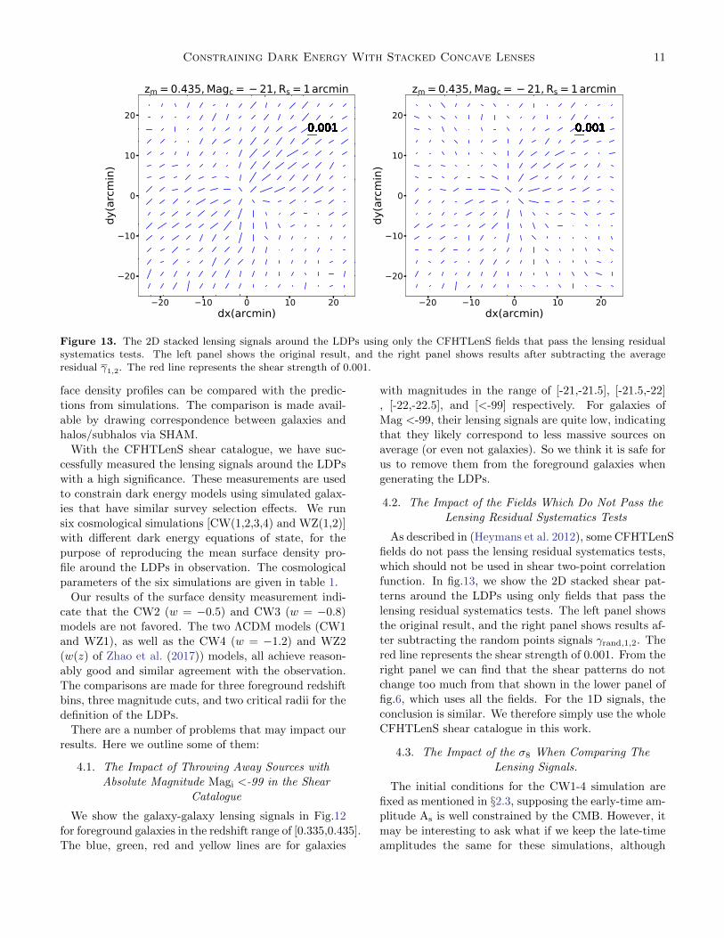
4.2. The Impact of the Fields Which Do Not Pass the

Lensing Residual Systematics Tests

As described in (Heymans et al. 2012), some CFHTLenS

fields do not pass the lensing residual systematics tests,

which should not be used in shear two-point correlation

function. In fig.13, we show the 2D stacked shear pat-

terns around the LDPs using only fields that pass the

lensing residual systematics tests. The left panel shows

the original result, and the right panel shows results af-

ter subtracting the random points signals γrand,1,2. The

red line represents the shear strength of 0.001. From the

right panel we can find that the shear patterns do not

change too much from that shown in the lower panel of

fig.6, which uses all the fields. For the 1D signals, the

conclusion is similar. We therefore simply use the whole

CFHTLenS shear catalogue in this work.

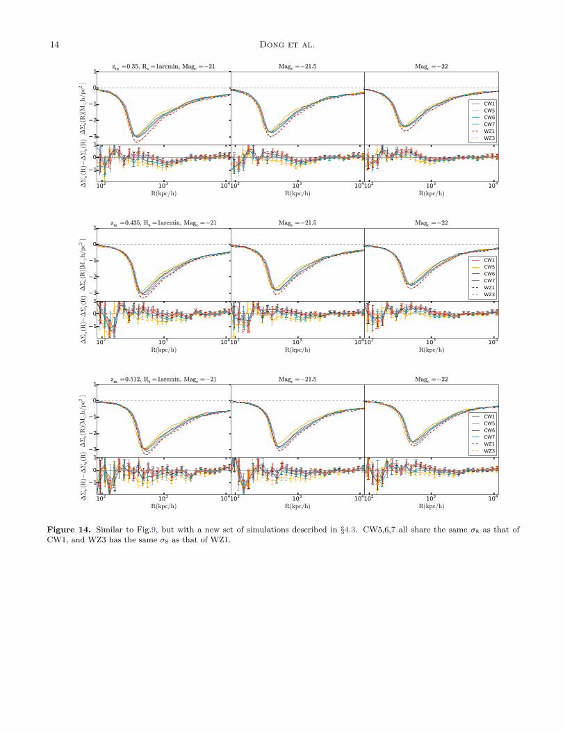
4.3. The Impact of the σ8 When Comparing The

Lensing Signals.

The initial conditions for the CW1-4 simulation are

fixed as mentioned in §2.3, supposing the early-time am-

plitude As is well constrained by the CMB. However, it

may be interesting to ask what if we keep the late-time

amplitudes the same for these simulations, although

12 Dong et al.

with very different As. So we run four new simulations

here as a comparison. Three new simulations are run for

the CW set, named as CW5,6,7. Also, one new simula-

tion is run for the WZ set, named as WZ3. For CW5,6,7,

the parameters (Ωc,Ωb,wde,h) are set the same as in

CW2,3,4 respectively, with the σ8 being the same as

that of CW1. For WZ3, its parameters(Ωc,Ωb,wde,h)

are identical with WZ2, with the σ8 taken from WZ1.

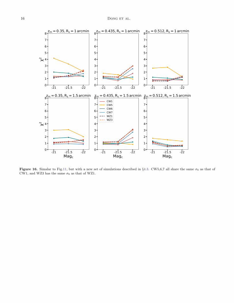
The parameters of the simulations are given in table 2.

All the procedures in §2.3 are repeated for the four

simulations. The simulated lensing signals around the

LDPs are compared with the observed signals in Fig.14

and Fig.15, which are similar to Fig.9 and 10. The

lensing profiles ∆Σs(R) for CW5,6,7 are found to be

close to each other. Although smaller compared to

Fig.9 and 10, discrepancies are still found for some cos-

mologies between the simulated and observed signals

in the lower panels. Their corresponding χ2 results

are shown in Fig.16. The CW5(w = −0.5) is found

to have larger χ2 than the others in most cases. The

χ2 of CW6(w = −0.8) seems to be slightly higher than

the rest. These results are redshift-dependent, and

the least distinguishable case is when zm = 0.435 and

Rs = 1.5 arcmin, in which different models result in com-

parable χ2.

Table 2. Simulation parameters.

Simulation wde σ8 Ωc Ωb h ns

CW5 -0.5 0.85 0.223 0.045 0.71 1

CW6 -0.8 0.85 0.223 0.045 0.71 1

CW7 -1.2 0.85 0.223 0.045 0.71 1

Simulation wde As Ωc Ωb h ns

WZ3 w(z) 2.16e-9 0.24188 0.04525 0.702 0.966

We note that our constraints on the dark energy

equation of state is still preliminary, in the sense that

we have fixed the values of the other cosmological pa-

rameters for simplicity. As a next step, we plan to vary

the cosmological model with more parameters, and fix

those that are best constrained by CMB. We also plan

to measure again the LDP lensing signals using the

Fourier Quad method (Zhang et al. 2017, 2018), which

is significantly different from the Lensfit method used by

the CFHTLenS team. Also, we are looking forward to

giving detailed discussions on the redshift evolution of

the LDP lensing signals with larger and deeper surveys7.

ACKNOWLEDGMENTS

This work is based on observations obtained with

MegaPrime/MegaCam, a joint project of CFHT and

CEA/DAPNIA, at the Canada-France-Hawaii Telescope

(CFHT) which is operated by the National Research

Council (NRC) of Canada, the Institut National des Sci-

ences de lUnivers of the Centre National de la Recherche

Scientifique (CNRS) of France, and the University of

Hawaii. This research used the facilities of the Cana-

dian Astronomy Data Centre operated by the National

Research Council of Canada with the support of the

Canadian Space Agency.

We thank Gongbo Zhao for providing us parameter

tables used for setting the WZ set simulations, Yipeng

Jing for providing us one of the CW1 simulation data,

and Pengjie Zhang for useful comments. This work

is supported by the National Key Basic Research and

Development Program of China (No.2018YFA0404504),

the National Key Basic Research Program of China

(2015CB857001, 2015CB857002), the NSFC grants

(11673016, 11433001, 11621303, 11773048, 11403071).

JXH is supported by JSPS Grant-in-Aid for Scientific

Research JP17K14271. JJZ is supported by China

Postdoctoral Science Foundation 2018M632097. LPF

acknowledges the support from NSFC grants 11673018,

11722326 & 11333001; STCSM grant 16ZR1424800 &

188014066; and SHNU grant DYL201603.

REFERENCES

Barreira, A., Bose, S., Li, B., & Llinares, C. 2017, JCAP, 2,

031

Behroozi, P. S., Conroy, C., & Wechsler, R. H. 2010, ApJ,

717, 379

Berlind, A. A., & Weinberg, D. H. 2002, ApJ, 575, 587

Brouwer, M. M., Demchenko, V., Harnois-Deraps, J., et al.

2018, MNRAS, 481, 5189

7 https://www.darkenergysurvey.org,https://www.desi.lbl.gov,https://www.lsst.org,http://www.sdss3.org/surveys/boss.php.

Ceccarelli, L., Padilla, N. D., Valotto, C., & Lambas, D. G.

2006, MNRAS, 373, 1440

Chaves-Montero, J., Angulo, R. E., Schaye, J., et al. 2016,

MNRAS, 460, 3100

Clampitt, J., & Jain, B. 2015, MNRAS, 454, 3357

Colberg, J. M., Sheth, R. K., Diaferio, A., Gao, L., &

Yoshida, N. 2005, MNRAS, 360, 216

Conroy, C., Gunn, J. E., & White, M. 2009, ApJ, 699, 486

Conroy, C., Wechsler, R. H., & Kravtsov, A. V. 2006, ApJ,

647, 201

https://www.darkenergysurvey.org

https://www.desi.lbl.gov

https://www.lsst.org

http://www.sdss3.org/surveys/boss.php.


Davies, C. T., Cautun, M., & Li, B. 2018, ArXiv e-prints,

arXiv:1803.08717

Elyiv, A., Marulli, F., Pollina, G., et al. 2015, MNRAS,

448, 642

Erben, T., Hildebrandt, H., Miller, L., et al. 2013, MNRAS,

433, 2545

Friedrich, O., Gruen, D., DeRose, J., et al. 2018, PhRvD,

98, 023508

Gruen, D., Friedrich, O., Amara, A., et al. 2016, MNRAS,

455, 3367

Gruen, D., Friedrich, O., Krause, E., et al. 2018, PhRvD,

98, 023507

Guo, H., Yang, X., & Lu, Y. 2018, ApJ, 858, 30

Guo, H., Zheng, Z., Behroozi, P. S., et al. 2016, MNRAS,

459, 3040

Guo, Q., & White, S. 2014, MNRAS, 437, 3228

Guo, Q., White, S., Li, C., & Boylan-Kolchin, M. 2010,

MNRAS, 404, 1111

Han, J., Frenk, C. S., Eke, V. R., et al. 2012, MNRAS, 427,

1651

Hartlap, J., Simon, P., & Schneider, P. 2007, A&A, 464, 399

Hearin, A. P., Zentner, A. R., Berlind, A. A., & Newman,

J. A. 2013, MNRAS, 433, 659

Heymans, C., Van Waerbeke, L., Miller, L., et al. 2012,

MNRAS, 427, 146

Hildebrandt, H., Erben, T., Kuijken, K., et al. 2012,

MNRAS, 421, 2355

Hoyle, F., & Vogeley, M. S. 2002, ApJ, 566, 641

Huterer, D., & Turner, M. S. 1999, PhRvD, 60, 081301

Jennings, E., Li, Y., & Hu, W. 2013, MNRAS, 434, 2167

Jing, Y. P., Mo, H. J., & Borner, G. 1998, ApJ, 494, 1

Jing, Y. P., Suto, Y., & Mo, H. J. 2007, ApJ, 657, 664

Komatsu, E., Bennett, C. L., Barnes, C., et al. 2014,

Progress of Theoretical and Experimental Physics, 2014,

06B102

Lavaux, G., & Wandelt, B. D. 2012, ApJ, 754, 109

Leauthaud, A., Tinker, J., Behroozi, P. S., Busha, M. T., &

Wechsler, R. H. 2011, ApJ, 738, 45

Lewis, A., Challinor, A., & Lasenby, A. 2000, Astrophys. J.,

538, 473

Li, B. 2011, MNRAS, 411, 2615

Miller, L., Heymans, C., Kitching, T. D., et al. 2013,

MNRAS, 429, 2858

Nadathur, S., Hotchkiss, S., Diego, J. M., et al. 2015,

MNRAS, 449, 3997

Neyrinck, M. C. 2008, MNRAS, 386, 2101

Niikura, H., Takada, M., Okabe, N., Martino, R., &

Takahashi, R. 2015, PASJ, 67, 103

Padilla, N. D., Ceccarelli, L., & Lambas, D. G. 2005,

MNRAS, 363, 977

Peacock, J. A. 1999, Cosmological Physics, 704

Perlmutter, S., Aldering, G., Goldhaber, G., et al. 1999,

ApJ, 517, 565

Planck Collaboration, Ade, P. A. R., Aghanim, N., et al.

2014, A&A, 571, A1

Platen, E., van de Weygaert, R., & Jones, B. J. T. 2007,

MNRAS, 380, 551

Ramos, B. H. F., Pellegrini, P. S., Benoist, C., et al. 2011,

AJ, 142, 41

Riess, A. G., Filippenko, A. V., Challis, P., et al. 1998, AJ,

116, 1009

Rodrıguez-Puebla, A., Avila-Reese, V., Yang, X., et al.

2015, ApJ, 799, 130

Rodrıguez-Puebla, A., Primack, J. R., Avila-Reese, V., &

Faber, S. M. 2017, MNRAS, 470, 651

Sanchez, C., Clampitt, J., Kovacs, A., et al. 2017, MNRAS,

465, 746

Simha, V., Weinberg, D. H., Dave, R., et al. 2012, MNRAS,

423, 3458

Springel, V. 2005, MNRAS, 364, 1105

Springel, V., & Hernquist, L. 2002, MNRAS, 333, 649

Taylor, A., Joachimi, B., & Kitching, T. 2013, MNRAS,

432, 1928

Vale, A., & Ostriker, J. P. 2004, MNRAS, 353, 189

—. 2006, MNRAS, 371, 1173

van den Bosch, F. C., Yang, X., Mo, H. J., et al. 2007,

MNRAS, 376, 841

Wechsler, R. H., & Tinker, J. L. 2018, ArXiv e-prints,

arXiv:1804.03097

Weinberg, D. H., Mortonson, M. J., Eisenstein, D. J., et al.

2013, PhR, 530, 87

Yang, X., Mo, H. J., & van den Bosch, F. C. 2003,

MNRAS, 339, 1057

Yang, X., Mo, H. J., van den Bosch, F. C., Zhang, Y., &

Han, J. 2012, ApJ, 752, 41

Yang, X., Zhang, Y., Wang, H., et al. 2018, ApJ, 860, 30

Zehavi, I., Zheng, Z., Weinberg, D. H., et al. 2011, ApJ,

736, 59

Zhang, J., Zhang, P., & Luo, W. 2017, ApJ, 834, 8

Zhang, J., Dong, F., Li, H., et al. 2018, ArXiv e-prints,

arXiv:1808.02593

Zhao, C., Tao, C., Liang, Y., Kitaura, F.-S., & Chuang,

C.-H. 2016, MNRAS, 459, 2670

Zhao, G.-B., Raveri, M., Pogosian, L., et al. 2017, Nature

Astronomy, 1, 627

Zheng, Z., Berlind, A. A., Weinberg, D. H., et al. 2005,

ApJ, 633, 791

Zu, Y., & Mandelbaum, R. 2016, MNRAS, 457, 4360

14 Dong et al.

r(kpc/h)

1

0

1

2

3

∆Σ

s(R

)[M

¯h/p

c2]


102 103 104

R(kpc/h)

1

0

1

∆Σ

o(R

)−∆

Σs(R

)

r(kpc/h)


102 103 104

R(kpc/h)

r(kpc/h)


CW1

CW5

CW6

CW7

WZ1

WZ3

102 103 104

R(kpc/h)

r(kpc/h)

1

0

1

2

3

∆Σ

s(R

)[M

¯h/pc2

]


102 103 104

R(kpc/h)

1

0

1

∆Σ

o(R

)−∆

Σs(R

)

r(kpc/h)


102 103 104

R(kpc/h)

r(kpc/h)


CW1

CW5

CW6

CW7

WZ1

WZ3

102 103 104

R(kpc/h)

r(kpc/h)

1

0

1

2

3

∆Σ

s(R

)[M

¯h/p

c2]


102 103 104

R(kpc/h)

1

0

1

∆Σ

o(R

)−∆

Σs(R

)

r(kpc/h)


102 103 104

R(kpc/h)

r(kpc/h)


CW1

CW5

CW6

CW7

WZ1

WZ3

102 103 104

R(kpc/h)

Figure 14. Similar to Fig.9, but with a new set of simulations described in §4.3. CW5,6,7 all share the same σ8 as that ofCW1, and WZ3 has the same σ8 as that of WZ1.


r(kpc/h)

1

0

1

2

3

4

∆Σ

s(R

)[M

¯h/p

c2]


102 103 104

R(kpc/h)

1

0

1

2

∆Σ

o(R

)−∆

Σs(R

)

r(kpc/h)


102 103 104

R(kpc/h)

r(kpc/h)


CW1

CW5

CW6

CW7

WZ1

WZ3

102 103 104

R(kpc/h)

r(kpc/h)

1

0

1

2

3

4

∆Σ

s(R

)[M

¯h/pc2

]


102 103 104

R(kpc/h)

1

0

1

2

∆Σ

o(R

)−∆

Σs(R

)

r(kpc/h)


102 103 104

R(kpc/h)

r(kpc/h)


CW1

CW5

CW6

CW7

WZ1

WZ3

102 103 104

R(kpc/h)

r(kpc/h)

1

0

1

2

3

4

∆Σ

s(R

)[M

¯h/p

c2]


102 103 104

R(kpc/h)

1

0

1

2

∆Σ

o(R

)−∆

Σs(R

)

r(kpc/h)


102 103 104

R(kpc/h)

r(kpc/h)


CW1

CW5

CW6

CW7

WZ1

WZ3

102 103 104

R(kpc/h)

Figure 15. Similar to fig.14, but with Rs = 1.5 arcmin.

16 Dong et al.

-21 -21.5 -220

1

2

3

4

5

6

7

8

2

zm = 0.35, Rs = 1 arcmin

-21 -21.5 -220

1

2

3

4

5

6

7

8zm = 0.435, Rs = 1 arcmin

-21 -21.5 -220

1

2

3

4

5

6

7

8zm = 0.512, Rs = 1 arcmin

-21 -21.5 -22Magc

0

1

2

3

4

5

6

7

8

2

zm = 0.35, Rs = 1.5 arcmin

-21 -21.5 -22Magc

0

1

2

3

4

5

6

7

8zm = 0.435, Rs = 1.5 arcminCW1CW5CW6CW7WZ1WZ3

-21 -21.5 -22Magc

0

1

2

3

4

5

6

7

8zm = 0.512, Rs = 1.5 arcmin

Figure 16. Simalar to Fig.11, but with a new set of simulations described in §4.3. CW5,6,7 all share the same σ8 as that ofCW1, and WZ3 has the same σ8 as that of WZ1.

draft version april 12, 2019 a twocolumn style in aastex62

Documents