droplet collision mixing diagnostics using single fluorophore lif
TRANSCRIPT
RESEARCH ARTICLE
Droplet collision mixing diagnostics using single fluorophore LIF
Brian Carroll • Carlos Hidrovo
Received: 19 December 2011 / Revised: 30 July 2012 / Accepted: 1 August 2012 / Published online: 19 August 2012
� Springer-Verlag 2012
Abstract A novel droplet mixing measurement technique
is presented that employs single fluorophore laser-induced
fluorescence, custom image processing, and statistical
analysis for monitoring and quantifying mixing in con-
fined, high-speed droplet collisions. The diagnostic proce-
dure captures time-varying fluorescent signals following
binary droplet collisions and reconstructs the spatial con-
centration field by relating fluorophore intensity to relative
concentration. Mixing information is revealed through two
governing statistics that separate the roles of convective
rearrangement and molecular diffusion during the mixing
process. The end result is a viewing window into the rich
dynamics of droplet collisions and a diagnostic tool that
differentiates between poor and effective mixing. The
technique has proved invaluable in the laboratory by
allowing direct comparison of different hydrodynamic
conditions, such as collision Reynolds and Peclet number,
and collision geometries, such as T and Y-junctions.
Experiments indicate improved mixing rates and degree of
homogenization as the convective timescale for the colli-
sion is decreased. Visualization of mixing residuals using
pseudo color mapping also identifies areas that are largely
segregated from the mixing process, resulting in islands
where mixing is poor and stirring has proved ineffective.
As the collision velocity is increased, vortical flow fields
become apparent and mixing is greatly improved.
1 Introduction
Mixing, dilution, or sample homogenization are an essential
process in modern lab-on-a-chip (LOC) and micro-total
analysis systems (lTAS) where this seemingly simple task
remains a major obstacle. The topic is forefront at any
microfluidics; conference or periodical and complete books
are devoted to the subject (Nguyen 2008). The ability to
analyze non-equilibrium conditions and probe the kinetics
of bio-molecular reactions has been limited by the speed at
which mixing takes place. The low Reynolds (Re) numbers
typical of most microfluidic devices signify laminar and
orderly flows that are devoid of any inertial characteristics.
The turbulent flow regime exploited at the macroscale
for fast mixing is difficult and impractical to implement
in microscale flows, although turbulent flow has been
achieved for continuous flow microfluidic devices
(Takahashi et al. 1995). Droplet-based systems offer sig-
nificant advantages over their continuous flow counterparts,
such as reduced product dispersion and sample consump-
tion and the ability to precisely control and monitor reac-
tions at desired timescales. However, the microsecond
mixing times that have been achieved for continuous flow
systems (Knight et al. 1998; Hertzog et al. 2004, 2006) are
two orders of magnitude smaller than the state of the art for
droplet-based systems (Song et al. 2003, 2006; Song and
Ismagilov 2003). Many important structural events, such as
nucleotide-flipping (Robinson et al. 2010) and calmodulin
(CaM) dynamics (Park et al. 2007), occur on timescales
much less than a millisecond. For droplet-based systems,
the most common fast mixing technique is chaotic advec-
tion. Chaotic advection produces highly divergent particle
motion inside droplet volumes using either active or passive
means. Regardless of the mixing technique, the overarching
goal is rapid and controllable reduction in the effective mass
B. Carroll (&) � C. Hidrovo
Multiscale Thermal Fluids Laboratory,
University of Texas at Austin, Austin, TX, USA
e-mail: [email protected]
C. Hidrovo
e-mail: [email protected]
123
Exp Fluids (2012) 53:1301–1316
DOI 10.1007/s00348-012-1361-x

diffusion length. The faster this length scale is reduced, the
faster the mixture is homogenized.
The difficulty in determining the extent or degree of
mixing is that there is no unifying theory that clearly dis-
tinguishes a ‘‘fully mixed’’ condition. Some (Ottino 1989,
1990, 1994; Dutta and Chevray 1994; Ottino and Wiggins
2004) have applied a Hamiltonian perspective to mixing
that describes well-mixed conditions if every particle
explores the mixing domain while losing track of each
other. This idea of particle divergence is the foundation of
chaotic mixing, a concept first pioneered by Aref (1984).
This purely dynamical approach to mixing is well suited
for high Peclet number laminar flows. Chemists describe
well-mixed conditions by the degree in which a chemical
reaction takes place, since a reaction cannot proceed unless
there are molecular interactions between the reactants
(Kling and Mewes 2010). This requires molecular scale
proximity. The turbulence community predicts mixed
conditions based on the homogenization of a scalar field,
such as concentration or temperature (Dimotakis et al.
1983; Koochesfahani and Dimotakis 1986; Dimotakis
2005). If homogenization is poor at the large scale, mixing
at the molecular scale will be highly localized and largely
poor throughout the volume. If homogenization is complete
at sub-system length scales, mixed conditions at the
molecular scale, although not guaranteed, may be safely
assumed. A mixing system displaying fast homogenization
rates at these intermediate, sub-system length scales
therefore provides molecularly mixed conditions faster
than a similarly scaled system displaying slow homogeni-
zation rates. Thus, quantifying the extent of mixing based
on concentration field homogenization provides an impor-
tant metric in mixing system performance and a benchmark
for system design. This report describes an optical diag-
nostic technique that employs laser-induced fluorescence
(LIF) using a single fluorophore, unique mixing statistics,
and custom image processing to quantify and visualize the
extent of mixing in confined droplet collisions.
This newly applied LIF measurement technique was
developed for mixing characterization of a recently pro-
posed inertial mixing device that increases droplet mixing
rates through high-speed collisions in a confined micro-
channel (Carroll and Hidrovo 2010, 2011). An easily
integrated, chemically inert diagnostic procedure was
sought that enables direct comparison of mixing occurring
at various inertial conditions The design capitalizes on a
rapid mixing technique presented by Simpson et al. (1983,
1986) where microdroplets are collided in an unconfined,
gaseous environment at high speed to yield mixing times
near 200 ls. Referring to the simplified schematic in
Fig. 1, liquid droplets of Solute 1 and 2 are detached and
accelerated by a high-speed gas flow from two opposing
legs of a T-junction. Each droplet obtains kinetic energy
KE1 and KE2 and surface energy SE1 and SE2. At the
common junction, the droplets collide and coalesce. The
kinetic and surface energy following collision is KE3 and
SE3, each of which is less than the respective energy prior
to collision. This abrupt change in kinetic and surface
energy is viscously dissipated through complex velocity
fields and bulk volumetric rearrangement. The result is near
millisecond mixing for nanoliter-sized droplets. Droplet
mixing through confined collisions distinguishes this
technique from droplet mixing achieved using boundary
interactions.
2 Background
The fast time scales, small length scales, and largely
Lagrangian nature of advanced droplet mixing techniques
make optical diagnostics the obvious choice for under-
standing, characterizing, and quantifying mixing dynamics.
Within the optical diagnostic tool box, three major tech-
niques have been successfully demonstrated: infrared
absorption (IR), spontaneous Raman scattering (SRS), and
LIF. IR techniques measure the wavelength and intensity of
mid-infrared (2.5–50 lm) light absorbed by a sample.
Energy provided by the light source excites molecular
vibrations to higher energy levels resulting in absorption
bands that are characteristic of specific types of chemical
bonds. SRS is an inelastic radiative scattering process that
operates on the short lived ‘‘virtual’’ states and subsequent
Raman shift. Both IR and SRS provide molecular finger-
prints of chemical species present in the investigation
region such that the local concentrations are resolved. LIF
is also an inelastic radiative process but is based on the
absorption and subsequent emission of a photon following
quantum energy state interactions. By controlling envi-
ronmental conditions and using spectral filtering, the LIF
signal can be used to construct a spatial concentration map
and provide mixing information.
KE1, SE
1
KE3 ~ 0
SE3< SE
1 + SE
2
KE2, SE
2
Solute 1 Solute 2
Gas Flow Gas Flow
Mixed Solutes
Fig. 1 Shown above is a simplified schematic of an inertial mixing
droplet collider. Two droplets with kinetic energy KE1 and KE2 and
surface energy SE1 and SE2 collide at a channel junction. The kinetic
energy following collision is essentially zero while the surface energy
SE3 is about 21/3 times less for equally sized spherical droplets. The
decrease in kinetic and surface energy is viscously dissipated inside
the droplet and quickly rearranges the contents for accelerated mixing
1302 Exp Fluids (2012) 53:1301–1316
123
The advantage and limitation of each method rests on
the process being investigated. Both IR and SRS suffer
from small collision cross sections and therefore produce
low-signal intensities unless high-power lasers are used.
Furthermore, IR has the disadvantage of line of sight
averaging where the received signal is axially integrated.
SRS requires a high degree of laser rejection in order to
separate the weak, inelastically scattered Raman light from
the intensely scattered Rayleigh light that lies close to the
laser line (Schrader et al. 1991). Additionally, IR and SRS
are a point- or line-based process and a special setup is
required to acquire information in two dimensions (Masca
et al. 2006; Jendrzok et al. 2010). LIF, on the other hand,
readily provides intensity information across a plane and,
depending on the optical systems used, only weakly inte-
grates the third dimension. Compared with IR and SRS,
LIF provides a significantly greater collision cross section
such that the excitation energy required for a detectable
signal is significantly less and in many cases a conventional
white light source is sufficient. The difficulty in discerning
mixing information using fluorescent intensity is that the
fluorescent emission signal is often dependent on envi-
ronmental conditions, such as temperature and pressure;
mixture conditions, such as pH; and excitation source
stability, such as temporal and spatial non-uniformities.
These variables attenuate and skew the concentration-
dependent signal such that mixing information is lost or
misleading. However, for investigating mixing in micro-
fluidic devices, LIF remains the most suitable method
given the small length and time scales and ease of system
integration.
LIF has heritage in many diverse science and engi-
neering applications. Initial success as a laser dye was
quickly advanced to a method for studying molecular
collisions and quantifying molecular concentrations with
detection efficiencies comparable to mass spectrometers at
that time (Kinsey 1977). Over the past four decades, LIF
has evolved into an invaluable optical diagnostic tool. It
has allowed investigation of complex structures not pos-
sible using other visualization techniques, such as mixture
composition in reacting and non-reacting shear layers
(Koochesfahani and Dimotakis 1986), turbulent jets
(Dimotakis, et al. 1983), and combustion processes
(Matsumoto et al. 1999). LIF allows spatial resolutions
greater than the light diffraction limit through Forster
Resonance Energy Transfer and has opened up new
opportunities in microbiology previously unachievable
(Quercioli 2011). The often complex dependence of fluo-
rescent intensity to mixture composition and environmental
conditions has allowed LIF measurements of temperature
(Anderson et al. 1998; Coppeta and Rogers 1998; Lavieille
et al. 2001; David et al. 2006), pressure (Hiller and Hanson
1988), pH levels (Bellerose and Rogers 1994; Coppeta and
Rogers 1998), film thickness (Coppeta et al. 1996; Hidrovo
and Hart 2001), velocity distribution functions (Jacobs
et al. 2007), and molecular level mixing (Bellerose and
Rogers 1994; Faes and Glasmacher 2010; Kling and Me-
wes 2010). The LIF application presented herein is the time
resolved microscopy visualization of spatial concentration
distributions and quantification of mixing homogenization
in droplets following high-speed collisions in a confined
microchannel. The focus is on passive mixing, where the
flow is unaffected by the scalar field yielding Level 1 type
mixing (Dimotakis 2005). A single fluorophore dye is used,
and the liquid volume illuminated remains at uniform
temperature and pH throughout the mixing event.
3 Technique fundamentals
3.1 Fluorescence
Since the emphasis of this manuscript is using LIF to
extract mixing information during droplet collisions, only a
brief, top-level account of the salient features of the LIF
process is provided below. The reader is referred to Arb-
eloa et al. (1998, 2005) for highly detailed photo-physical
and chemical descriptions and Quercioli (2011) for a
comprehensive review of fluorescence and its applications
in modern microscopy. Fluorescence occurs when a spe-
cific type of molecule, called a fluorophore, is excited by a
photon and undergoes inelastic rotational and vibrational
losses before emitting a photon of longer wavelength and
returning to the ground state. Photon emission can be
reduced, entirely suppressed, or spectrally altered through
non-radiative quenching processes. Such processes include
imposed chemical reactions (Ware 1962; Knight et al.
1998; Kling and Mewes 2010), self-quenching due to
collisions with like molecules (MacDonald 1990), or spe-
cie-dependent bathochromic shifts in the fluorescent band
(Arbeloa et al. 2005). For the diagnostic technique pre-
sented here, no chemical reactions are imposed or con-
sidered and only the self-quenching process is recognized
as a possible path for fluorescent attenuation.
As light propagates through a participating medium its
intensity decays with distance. The rate of decay is
dependent on the spectral properties of the incident light
and absorption properties of the participating medium.
Water, for instance, preferentially absorbs longer wave-
length red light to a greater degree than shorter wavelength
blue light. In the case of a fluorescing substance, the
absorbed shorter wavelength intensity is released as longer
wavelength fluorescence. However, the process is inelastic
and only a fraction of the absorbed excitation energy is
emitted as fluorescence. The quantum yield of the process
is the ratio of emitted fluorescence intensity to absorbed
Exp Fluids (2012) 53:1301–1316 1303
123
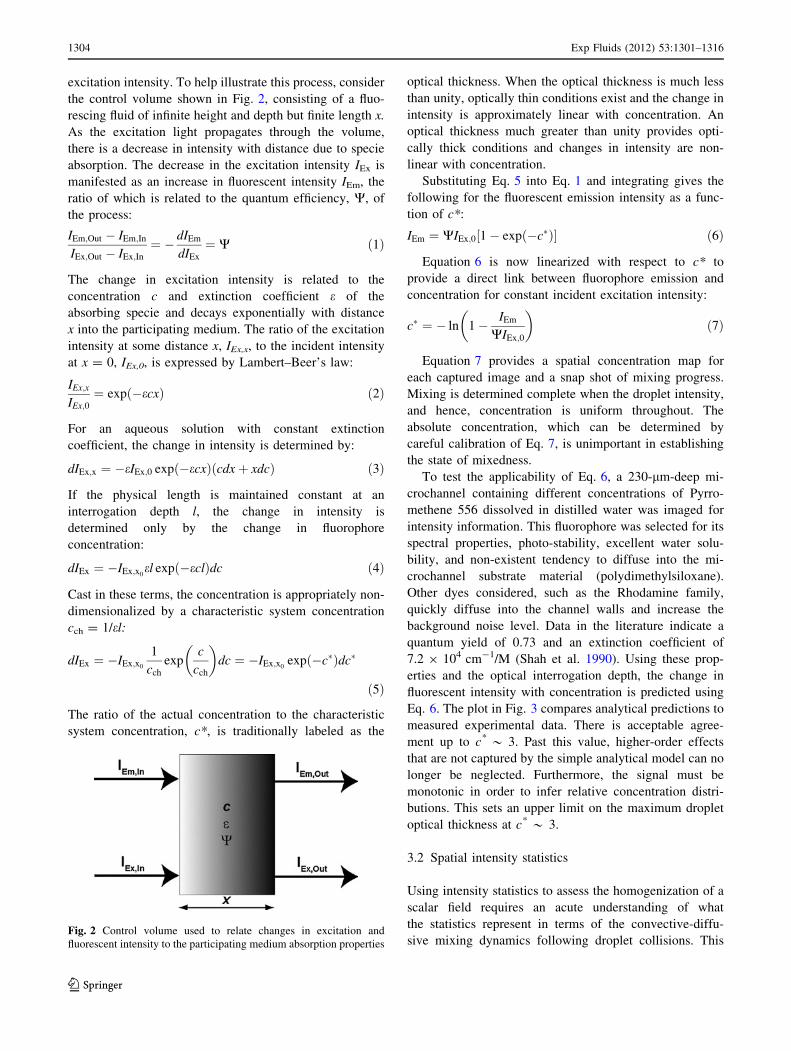
excitation intensity. To help illustrate this process, consider
the control volume shown in Fig. 2, consisting of a fluo-
rescing fluid of infinite height and depth but finite length x.
As the excitation light propagates through the volume,
there is a decrease in intensity with distance due to specie
absorption. The decrease in the excitation intensity IEx is
manifested as an increase in fluorescent intensity IEm, the
ratio of which is related to the quantum efficiency, W, of
the process:
IEm;Out � IEm;In
IEx;Out � IEx;In¼ � dIEm
dIEx
¼ W ð1Þ
The change in excitation intensity is related to the
concentration c and extinction coefficient e of the
absorbing specie and decays exponentially with distance
x into the participating medium. The ratio of the excitation
intensity at some distance x, IEx,x, to the incident intensity
at x = 0, IEx,0, is expressed by Lambert–Beer’s law:
IEx;x
IEx;0¼ exp �ecxð Þ ð2Þ
For an aqueous solution with constant extinction
coefficient, the change in intensity is determined by:
dIEx;x ¼ �eIEx;0 exp �ecxð Þ cdxþ xdcð Þ ð3Þ
If the physical length is maintained constant at an
interrogation depth l, the change in intensity is
determined only by the change in fluorophore
concentration:
dIEx ¼ �IEx;x0el exp �eclð Þdc ð4Þ
Cast in these terms, the concentration is appropriately non-
dimensionalized by a characteristic system concentration
cch = 1/el:
dIEx ¼ �IEx;x0
1
cch
expc
cch
� �dc ¼ �IEx;x0
exp �c�ð Þdc�
ð5Þ
The ratio of the actual concentration to the characteristic
system concentration, c*, is traditionally labeled as the
optical thickness. When the optical thickness is much less
than unity, optically thin conditions exist and the change in
intensity is approximately linear with concentration. An
optical thickness much greater than unity provides opti-
cally thick conditions and changes in intensity are non-
linear with concentration.
Substituting Eq. 5 into Eq. 1 and integrating gives the
following for the fluorescent emission intensity as a func-
tion of c*:
IEm ¼ WIEx;0 1� exp �c�ð Þ½ � ð6Þ
Equation 6 is now linearized with respect to c* to
provide a direct link between fluorophore emission and
concentration for constant incident excitation intensity:
c� ¼ � ln 1� IEm
WIEx;0
� �ð7Þ
Equation 7 provides a spatial concentration map for
each captured image and a snap shot of mixing progress.
Mixing is determined complete when the droplet intensity,
and hence, concentration is uniform throughout. The
absolute concentration, which can be determined by
careful calibration of Eq. 7, is unimportant in establishing
the state of mixedness.
To test the applicability of Eq. 6, a 230-lm-deep mi-
crochannel containing different concentrations of Pyrro-
methene 556 dissolved in distilled water was imaged for
intensity information. This fluorophore was selected for its
spectral properties, photo-stability, excellent water solu-
bility, and non-existent tendency to diffuse into the mi-
crochannel substrate material (polydimethylsiloxane).
Other dyes considered, such as the Rhodamine family,
quickly diffuse into the channel walls and increase the
background noise level. Data in the literature indicate a
quantum yield of 0.73 and an extinction coefficient of
7.2 9 104 cm-1/M (Shah et al. 1990). Using these prop-
erties and the optical interrogation depth, the change in
fluorescent intensity with concentration is predicted using
Eq. 6. The plot in Fig. 3 compares analytical predictions to
measured experimental data. There is acceptable agree-
ment up to c* * 3. Past this value, higher-order effects
that are not captured by the simple analytical model can no
longer be neglected. Furthermore, the signal must be
monotonic in order to infer relative concentration distri-
butions. This sets an upper limit on the maximum droplet
optical thickness at c* * 3.
3.2 Spatial intensity statistics
Using intensity statistics to assess the homogenization of a
scalar field requires an acute understanding of what
the statistics represent in terms of the convective-diffu-
sive mixing dynamics following droplet collisions. ThisFig. 2 Control volume used to relate changes in excitation and
fluorescent intensity to the participating medium absorption properties
1304 Exp Fluids (2012) 53:1301–1316
123

understanding is facilitated by considering the simple set
of images in Fig. 4, each a 400 9 400 pixel array. The
pixel intensity values range from 1 (white) to 0 (black)
with 256 discrete intensity values (8 bit images). Using
the first image in the upper left corner as the initial state
of a captured intensity field, two distinct processes can
occur: pure convective rearrangement (top row, left to
right) or pure diffusion (top row, top to bottom). Con-
vective motion rearranges the contents while maintaining
the same discrete intensity values, much like shaking
black and white marbles in a can. The images along the
top row represent 2, 4, 16, and 64 spatial divisions,
respectively. Diffusion maintains the same arrangement
but smears the intensity values at the interfaces. To
simulate the effects of diffusion, each interior pixel was
assigned a new value based on the average intensity of
the top, bottom, right, and left neighboring pixels. Starting
from the top row of images, each lower image has been
spatially averaged 101, 103, and 104 times, respectively.
Actual mixing follows a combination of convection and
diffusion motion that act in parallel. Fluid properties
(Schmidt number) and flow regime (Reynolds number)
determine the dominance of one path over the other.
Regardless of path taken, visual observation reveals a
‘‘more mixed’’ scalar field as compared to the initial state.
It is the objective of the selected statistics to quantify this
qualitative visual change in the scalar field.
The statistics that capture the visual representation of
scalar mixing are the mean and standard deviation of the
global intensity field (system level) and the average
gradient of the intensity field (local level). The theoreti-
cal expected value of a continuous planar intensity distri-
bution is:
lT ¼R
A IdA
Að8Þ
For digitized images, the intensity values are spatially
discrete and the area integral is replaced with a summation
over all N pixels inside the mixing volume:
l ¼PN
i¼1 Ii
Nð9Þ
In regards to the images in Fig. 4, the expected value is 0.5
for each image regardless of the mixing path. The average
intensity for a closed system, much like the average con-
centration, is a conserved quantity.
The standard deviation of the intensity field provides a
measure of how the spatial intensity values deviate from
the expected value l. In terms of mixing, it is a metric for
determining the dispersion of the intensity field. The the-
oretical standard deviation for a continuous distribution is:
rT ¼R
A ðI � lÞ2dA
A
" #12
ð10Þ
For discretized samples, the standard deviation is:
r ¼PN
i¼1 Ii � lð Þ2
N � 1
" #12
ð11Þ
Since the standard deviation is essentially a measuring stick
for variability, it is important to place this measurement in
Fig. 3 A comparison of experimental data (points) and analytical
prediction (line) of Pyrromethene 556 fluorescent emission. There is
good agreement up to c* * 3, after which self-quenching and other
higher-order effects not included in the simple analytical model begin
to take effectFig. 4 A series of simple gray scale images that illustrate the role of
convection and diffusion in mixing. Each of the 16 images is a
400 9 400 pixel array. Starting from the initial distribution in the
upper left corner, the pixels can be convectively rearranged by 22, 24,
and 26 times (upper row) or diffusively averaged 101, 103, and 104
times (left column). The remaining three columns represent the same
diffusive mixing but starting from a more convectively rearranged
state
Exp Fluids (2012) 53:1301–1316 1305
123
context with the system being investigated. The standard
deviation alone is meaningless without knowledge of the
expected value. For instance, a standard deviation of 0.5 for a
sample mean of 50 indicates little variability compared with
a system with a sample mean of 1. Another complication in
using Eq. 9 directly is the dependence of the standard
deviation to the magnitude of the intensity values. If results
are obtained using an exposure of 10 ls and compared with
results using an exposure of 1 ls, the standard deviation
would differ even though the actual mixing may be
unchanged. This is due to the larger intensity values
obtained for slower exposures. Normalizing the standard
deviation by the mean value remedies both these issues:
rl¼
PNi¼1
Ii
l � 1� �2
N � 1
264
375
12
ð12Þ
The normalized standard deviation is an excellent metric
for purely diffusive processes, such as that shown in the
column of images where initially the black and white
distribution is smeared to a greater degree of gray at the
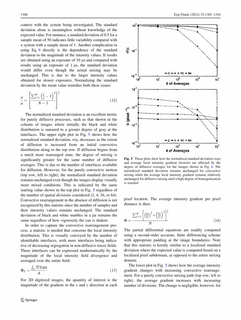
interfaces. The upper right plot in Fig. 5 shows how the
normalized standard deviation, r/l, decreases as the extent
of diffusion is increased from an initial convective
distribution along to the top row. If diffusion begins from
a much more rearranged state, the degree of mixing is
significantly greater for the same number of diffusive
averages. This is due to the number of interfaces available
for diffusion. However, for the purely convective motion
(top row, left to right), the normalized standard deviation
remains unchanged even though the images display visually
more mixed conditions. This is indicated by the same
starting value shown in the top plot in Fig. 5 regardless of
the number of spatial divisions considered (2, 4, 16, or 64).
Convective rearrangement in the absence of diffusion is not
recognized by this statistic since the number of samples and
their intensity values remains unchanged. The standard
deviation of black and white marbles in a jar remains the
same regardless of how vigorously the can is shaken.
In order to capture the convective rearrangement pro-
cess, a statistic is needed that concerns the local intensity
distribution. This is visually conveyed by the number of
identifiable interfaces, with more interfaces being indica-
tive of decreasing segregation in non-diffusive tracer fields.
These interfaces can be expressed mathematically by the
magnitude of the local intensity field divergence and
averaged over the entire field:
UT ¼R
A rIj jdA
Að13Þ
For 2D digitized images, the quantity of interest is the
magnitude of the gradient in the x and y direction at each
pixel location. The average intensity gradient per pixel
distance is then:
U ¼
PNi¼1
oIi
ox
� �2þ oIi
oy
� �2� 1
2
Nð14Þ
The partial differential equations are readily computed
using a second-order accurate, finite differencing scheme
with appropriate padding at the image boundaries. Note
that this statistic is keenly similar to a localized standard
deviation where the expected value is computed based on a
localized pixel subdomain, as opposed to the entire mixing
domain.
The lower plot in Fig. 5 shows how the average intensity
gradient changes with increasing convective rearrange-
ment. For a purely convective mixing path (top row, left to
right), the average gradient increases with increasing
number of divisions. The change is negligible, however, for
Fig. 5 These plots show how the normalized standard deviation (top)
and average local intensity gradient (bottom) are affected by the
degree of diffusive averages for the images shown in Fig. 4. The
normalized standard deviation remains unchanged for convective
mixing while the average local intensity gradient remains relatively
unchanged for diffusive mixing until a high degree of homogenization
is reached
1306 Exp Fluids (2012) 53:1301–1316
123

a purely diffusive process that begins highly segregated,
such as that given by the first two columns of images (2 and
4 divisions). If diffusion begins from a more rearranged
state, the average gradient decreases by 2–3 decades (16
and 64 divisions). These results show that convective and
diffusive action has opposite effects on the average inten-
sity gradient. It is the role of convection and diffusion to
create and smear gradients, respectively. A potentially
hazardous interpretation of the average gradient is that a
decreasing trend must signify diffusive action. The average
gradient continues to grow with increasing convective
rearrangement but only until the length scale of each pixel
is larger than the actual distance over which the gradient
occurs. Even in the absence of diffusion, the average gra-
dient will decrease once the spatial resolution of the
measurement system is exceeded.
It is evident based on these simple cases that the stan-
dard deviation captures diffusive mixing well but does not
recognize spatial rearrangement. This missing metric is
provided by the average local gradient that recognizes
stirring contributions. Because mixing in most processes of
interest is a combination of convective and diffusive paths,
using only a single statistic does not provide a complete
picture of the mixing event. These two statistics together
provide a window into the simultaneous process of con-
vective-diffusive mixing.
3.3 Droplet volume tracking
One of the challenges in applying these statistics to droplet
mixing is identification of the droplet volumes, which do
not fill the entire image frame and translate across the
frame throughout the mixing event. In order to locate each
droplet prior to collision, both droplets must emit a
detectable signal while maintaining sufficient intensity
difference to make the statistics meaningful. This is over-
come by using fluorophore concentrations that are an order
of magnitude different between the two droplets prior to
collision. The captured frames are exported in tagged
image format (TIFF) at 12 bit resolution (4,096 intensity
levels) and converted to double precision values between 0
and 1. A custom image processing code is executed in
MATLAB� to spatially identify the droplet volumes for
each frame. The locating algorithm is a combination of
noise reduction, local intensity spatial derivatives, intensity
thresholding, and shape filling numerical techniques. This
process produces a binary region of interest (ROI) mask
that is used for confining the mixing statistics to the liquid
droplet volumes only. The pairs of images in Fig. 6 illus-
trate the binary ROI process for an actual mixing event and
highlight the volume tracking process. A single droplet of
high fluorophore concentration (high intensity) is perched
at the apex of a Y-junction (image pair 1). A second droplet
Fig. 6 A series of images of an actual mixing event that illustrates
the image processing technique used to identify each droplet volume.
Each raw image (left) is accompanied by the corresponding binary
image (right) that shows the droplets in white and clearly identifies
the droplet volumes throughout the mixing event. The image
sequence shows a droplet perched at the Y-junction apex while
second droplet is approaching from lower right (1), the moment just
prior to collision (2), the moment just after collision indicating
intensity gradient development (3), and the mixing dynamics 1 ms
after collision showing the formation of a single vortex with counter-
clockwise rotation (4)
Exp Fluids (2012) 53:1301–1316 1307
123

of lower fluorophore concentration (low intensity) approa-
ches from the lower right (image pair 2) and collides with
the first droplet (image pair 3). Mixing takes place within
the coalescing droplet (image pair 4). Note the presence of a
counter-rotating vortex that is generated as a result of the
collision.
4 Experimental setup
The droplet collision mixing device used to demonstrate
this diagnostic procedure consists of a T-junction for
droplet generation and a Y-junction for droplet collisions.
A high-speed air flow (10–20 m/s) is used to create
droplets from two liquid streams at opposing T-junctions
using techniques previously investigated (Carroll and Hi-
drovo 2009). The discrete droplets are entrained and
transported by the gaseous continuous phase to a common
Y-junction where collisions take place at relative velocities
near 0.1–1 m/s. The newly coalesced and mixed droplet is
then removed from the junction along a common channel,
readying the Y-junction for the next colliding droplet pair.
Each opposing channel leg is 100 lm wide and the exit
channel is 200 lm wide. The depth of each channel is
approximately 100 lm. A schematic of the mixing device
is shown in Fig. 7. Provided are image sequences that
capture the detachment and collision events. The bottom
image series shows the growth and detachment of a single
Liquid Flow
Gas Flow
Fig. 7 Top-view CAD schematic of the impact coalescence mixing
device accompanying experimental images depicting a collision
mixing event (top) and the droplet growth and detachment process
(bottom). The droplet collider uses a high-speed gaseous flow to
detach discrete droplets at T-junction. Entrained droplets from two
opposing legs are brought together at the apex of a Y-junction.
Mixing takes place rapidly and the newly coalesced droplet is
removed by the gas flow down a common exit channel
1308 Exp Fluids (2012) 53:1301–1316
123
droplet from the left T-junction. In top image sequence,
two droplets of high (right) and low (left) fluorophore
concentration collide, mix, and exit the junction. Note the
difference in intensity of each droplet prior to collision,
which is representative of fluorophore concentration.
The impact coalescence mixing device shown in Fig. 7
is microfabricated using standard soft lithography tech-
niques and polydimethylsiloxane (PDMS, Dow Corning
Corp.) substrate material. Each PDMS mixing device is
bonded using oxygen plasma to a 100 9 300 standard
microscope slide that has been spin coated with a *5-lm
thick layer of PDMS. This ensures all channel walls display
the same surface energy and wetting characteristics. Bond
strength is improved by post-baking at 65 �C for 8 h. The
finished device is then inspected for dimensional integrity
using a microscope and checked for leaks using a pressure
source and flow meter.
A custom microfluidic test bed has been designed for
experimental investigation of multiphase flows, particu-
larly high-speed gas–liquid droplet flows. The test bed
consists of pairs of pressure transducers (Validyne P855
Digital Differential Pressure Transmitter) and mass flow
sensors (Sierra Smart-Trak2) for real-time data acquisition.
Gas flow control is realized using voltage-driven pressure
regulators (Proportion-Air QPV1) with feedback control.
Compressed air supplied by the facility is oil and particu-
late filtered and desiccated upstream before being intro-
duced into the pressure regulator. Back pressure is
achieved using a 20-turn needle valve (McMaster Carr).
Liquid flow control is provided by a constant displacement
syringe pump (Harvard Apparatus PHD2000). All instru-
ments and acquisition equipment are routed through a
dedicated host computer. A custom LabVIEW Virtual
Instrument (National Instruments) provides real-time user
control and system diagnostics of all instrumentation.
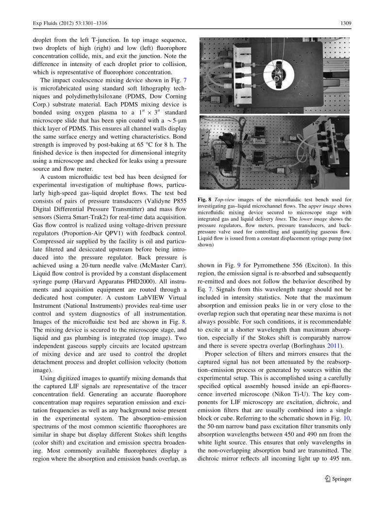
Images of the microfluidic test bed are shown in Fig. 8.
The mixing device is secured to the microscope stage, and
liquid and gas plumbing is integrated (top image). Two
independent gaseous supply circuits are located upstream
of mixing device and are used to control the droplet
detachment process and droplet collision velocity (bottom
image).
Using digitized images to quantify mixing demands that
the captured LIF signals are representative of the tracer
concentration field. Generating an accurate fluorophore
concentration map requires separation emission and exci-
tation frequencies as well as any background noise present
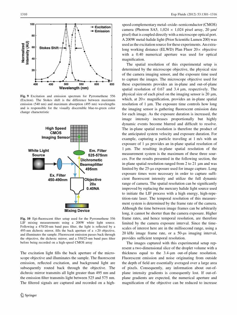
in the experimental system. The absorption–emission
spectrums of the most common scientific fluorophores are
similar in shape but display different Stokes shift lengths
(color shift) and excitation and emission spectra broaden-
ing. Most commonly available fluorophores display a
region where the absorption and emission bands overlap, as
shown in Fig. 9 for Pyrromethene 556 (Exciton). In this
region, the emission signal is re-absorbed and subsequently
re-emitted and does not follow the behavior described by
Eq. 7. Signals from this wavelength range should not be
included in intensity statistics. Note that the maximum
absorption and emission peaks lie in or very close to the
overlap region such that operating near these maxima is not
always possible. For such conditions, it is recommendable
to excite at a shorter wavelength than maximum absorp-
tion, especially if the Stokes shift is comparably narrow
and there is severe spectra overlap (Borlinghaus 2011).
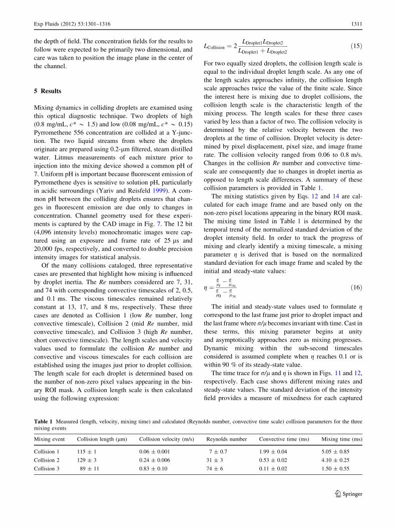
Proper selection of filters and mirrors ensures that the
captured signal has not been attenuated by the reabsorp-
tion–emission process or generated by sources within the
experimental setup. This is accomplished using a carefully
specified optical assembly housed inside an epi-fluores-
cence inverted microscope (Nikon Ti-U). The key com-
ponents for LIF microscopy are excitation, dichroic, and
emission filters that are usually combined into a single
block or cube. Referring to the schematic shown in Fig. 10,
the 50-nm narrow band pass excitation filter transmits only
absorption wavelengths between 450 and 490 nm from the
white light source. This ensures that only wavelengths in
the non-overlapping absorption band are transmitted. The
dichroic mirror reflects all incoming light up to 495 nm.
Fig. 8 Top-view images of the microfluidic test bench used for
investigating gas–liquid microchannel flows. The upper image shows
microfluidic mixing device secured to microscope stage with
integrated gas and liquid delivery lines. The lower image shows the
pressure regulators, flow meters, pressure transducers, and back-
pressure valve used for controlling and quantifying gaseous flow.
Liquid flow is issued from a constant displacement syringe pump (not
shown)
Exp Fluids (2012) 53:1301–1316 1309
123
The excitation light fills the back aperture of the micro-
scope objective and illuminates the sample. The fluorescent
emission, reflected excitation, and background light are
subsequently routed back through the objective. The
dichroic mirror transmits all light greater than 495 nm and
the emission filter transmits light between 525 and 575 nm.
The filtered signals are captured and recorded on a high-
speed complementary metal–oxide–semiconductor (CMOS)
camera (Photron SA5, 1,024 9 1,024 pixel array, 20 lm/
pixel) that is coupled directly with a microscope optical port.
A 200W metal-halide light (Prior Scientific Lumen 200) was
used as the excitation source for these experiments. An extra-
long working distance (ELWD) Plan Fluor 209 objective
with a 0.40 numerical aperture was used for optical
magnification.
The spatial resolution of this experimental setup is
determined by the microscope objective, the physical size
of the camera imaging sensor, and the exposure time used
to capture the images. The microscope objective used for
these experiments provides an in-plane and out-of-plane
spatial resolution of 0.67 and 3.4 lm, respectively. The
physical size of each pixel on the imaging sensor is 20 lm,
which, at 209 magnification, provides an in-plane spatial
resolution of 1 lm. The exposure time controls how long
the imaging sensor is gathering fluorescent emission data
for each image. As the exposure duration is increased, the
image intensity increases proportionally but highly
dynamic events become blurred and difficult to resolve.
The in-plane spatial resolution is therefore the product of
the anticipated system velocity and exposure duration. For
example, capturing a particle traveling at 1 m/s with an
exposure of 1 ls provides an in-plane spatial resolution of
1 lm. The resulting in-plane spatial resolution of the
measurement system is the maximum of these three sour-
ces. For the results presented in the following section, the
in-plane spatial resolution ranged from 2 to 21 lm and was
limited by the 25-ls exposure used for image capture. Long
exposure times were necessary in order to capture suffi-
cient fluorescent intensity and utilize the full dynamic
range of camera. The spatial resolution can be significantly
improved by replacing the mercury halide light source used
to initiate the LIF process with a high energy, high-repe-
tition-rate laser. The temporal resolution of this measure-
ment system is determined by the frame rate of the camera.
Although the time between image frames can be arbitrarily
long, it cannot be shorter than the camera exposure. Higher
frame rates, and hence temporal resolution, are therefore
limited by the camera exposure interval. Since the time-
scales of interest here are in the millisecond range, using a
20 kHz image frame rate, or a 50-ls imaging interval,
provides sufficient temporal resolution.
The images captured with this experimental setup rep-
resent a two-dimensional slice of the droplet volume with a
thickness equal to the 3.4-lm out-of-plane resolution.
Fluorescent emission and noise originating from outside
the depth of field are essentially averaged over a large area
of pixels. Consequently, any information about out-of-
plane intensity gradients is consequently lost. If out-of-
plane gradients are expected, the numerical aperture and
magnification of the objective can be reduced to increase
Fig. 9 Excitation and emission spectrum for Pyrromethene 556
(Exciton). The Stokes shift is the difference between maximum
emission (540 nm) and maximum absorption (495 nm) wavelengths
and is responsible for the visually discernible blue-to-green color
change characteristic
Fig. 10 Epi-fluorescent filter setup used for the Pyrromethene 556
LIF mixing measurements using a 200W white light source.
Following a 470/20-nm band pass filter, the light is reflected by a
495-nm dichroic mirror, fills the back aperture of a 920 objective,
and illuminates the sample. Fluorescent emission passes back through
the objective, the dichroic mirror, and a 550/25-nm band pass filter
before being recorded on a high-speed CMOS array
1310 Exp Fluids (2012) 53:1301–1316
123
the depth of field. The concentration fields for the results to
follow were expected to be primarily two dimensional, and
care was taken to position the image plane in the center of
the channel.
5 Results
Mixing dynamics in colliding droplets are examined using
this optical diagnostic technique. Two droplets of high
(0.8 mg/mL, c* * 1.5) and low (0.08 mg/mL, c* * 0.15)
Pyrromethene 556 concentration are collided at a Y-junc-
tion. The two liquid streams from where the droplets
originate are prepared using 0.2-lm filtered, steam distilled
water. Litmus measurements of each mixture prior to
injection into the mixing device showed a common pH of
7. Uniform pH is important because fluorescent emission of
Pyrromethene dyes is sensitive to solution pH, particularly
in acidic surroundings (Yariv and Reisfeld 1999). A com-
mon pH between the colliding droplets ensures that chan-
ges in fluorescent emission are due only to changes in
concentration. Channel geometry used for these experi-
ments is captured by the CAD image in Fig. 7. The 12 bit
(4,096 intensity levels) monochromatic images were cap-
tured using an exposure and frame rate of 25 ls and
20,000 fps, respectively, and converted to double precision
intensity images for statistical analysis.
Of the many collisions cataloged, three representative
cases are presented that highlight how mixing is influenced
by droplet inertia. The Re numbers considered are 7, 31,
and 74 with corresponding convective timescales of 2, 0.5,
and 0.1 ms. The viscous timescales remained relatively
constant at 13, 17, and 8 ms, respectively. These three
cases are denoted as Collision 1 (low Re number, long
convective timescale), Collision 2 (mid Re number, mid
convective timescale), and Collision 3 (high Re number,
short convective timescale). The length scales and velocity
values used to formulate the collision Re number and
convective and viscous timescales for each collision are
established using the images just prior to droplet collision.
The length scale for each droplet is determined based on
the number of non-zero pixel values appearing in the bin-
ary ROI mask. A collision length scale is then calculated
using the following expression:
LCollision ¼ 2LDroplet1LDroplet2
LDroplet1 þ LDroplet2
ð15Þ
For two equally sized droplets, the collision length scale is
equal to the individual droplet length scale. As any one of
the length scales approaches infinity, the collision length
scale approaches twice the value of the finite scale. Since
the interest here is mixing due to droplet collisions, the
collision length scale is the characteristic length of the
mixing process. The length scales for these three cases
varied by less than a factor of two. The collision velocity is
determined by the relative velocity between the two
droplets at the time of collision. Droplet velocity is deter-
mined by pixel displacement, pixel size, and image frame
rate. The collision velocity ranged from 0.06 to 0.8 m/s.
Changes in the collision Re number and convective time-
scale are consequently due to changes in droplet inertia as
opposed to length scale differences. A summary of these
collision parameters is provided in Table 1.
The mixing statistics given by Eqs. 12 and 14 are cal-
culated for each image frame and are based only on the
non-zero pixel locations appearing in the binary ROI mask.
The mixing time listed in Table 1 is determined by the
temporal trend of the normalized standard deviation of the
droplet intensity field. In order to track the progress of
mixing and clearly identify a mixing timescale, a mixing
parameter g is derived that is based on the normalized
standard deviation for each image frame and scaled by the
initial and steady-state values:
g ¼rlt� r
l1rl0� r
l1ð16Þ
The initial and steady-state values used to formulate gcorrespond to the last frame just prior to droplet impact and
the last frame where r/l becomes invariant with time. Cast in
these terms, this mixing parameter begins at unity
and asymptotically approaches zero as mixing progresses.
Dynamic mixing within the sub-second timescales
considered is assumed complete when g reaches 0.1 or is
within 90 % of its steady-state value.
The time trace for r/l and g is shown in Figs. 11 and 12,
respectively. Each case shows different mixing rates and
steady-state values. The standard deviation of the intensity
field provides a measure of mixedness for each captured
Table 1 Measured (length, velocity, mixing time) and calculated (Reynolds number, convective time scale) collision parameters for the three
mixing events
Mixing event Collision length (lm) Collision velocity (m/s) Reynolds number Convective time (ms) Mixing time (ms)
Collision 1 115 ± 1 0.06 ± 0.001 7 ± 0.7 1.99 ± 0.04 5.05 ± 0.85
Collision 2 129 ± 3 0.24 ± 0.006 31 ± 3 0.53 ± 0.02 4.10 ± 0.25
Collision 3 89 ± 11 0.83 ± 0.10 74 ± 6 0.11 ± 0.02 1.50 ± 0.55
Exp Fluids (2012) 53:1301–1316 1311
123

image frame. The statistic decreases from its initial value
just prior to collision and achieves a new value that remains
relatively invariant under the timescales considered. The
results show decreased intensity residuals for collisions
occurring at higher relative velocities where increased
rearrangement occurs. This is supported by inspection of
the simple images shown in Fig. 4 and resulting standard
deviation traces in Fig. 5. Note that, for a given number of
diffusive averages, the standard deviation is significantly
less if starting from a more rearranged state.
The decay rate is an indication of how quickly diffusion
is homogenizing the concentration field. The rate is faster if
diffusion begins from a more rearranged state since the
number of interfaces is greatly increased. Collisions
occurring at higher relative velocity produce greater
volumetric rearrangement, that is, analogous to shaking a
can of marbles with greater vigor. The kinetic energy
carried by each droplet is viscously dissipated through
complex velocity gradients within the liquid volume that
help create concentration interfaces for mass diffusion. The
length scale of the collision also plays an important role.
When shaken at the same rate, a single marble is more
likely to sample the entire can volume as compared to the
same marble in a much larger can. This difference is
captured by the convective timescale of the event. The ratio
of actual mixing time to the convective timescale of the
collision provides a convenient measure to distinguish the
role of convective stirring in mixing. This ratio increased
non-linearly with Re number from 2.5 for Collision 1 to
13.8 for Collision 3 as shown in Fig. 13 and supports the
trend of results previously obtained for a different collision
geometry (Carroll and Hidrovo 2012).
The other mixing statistic of interest is the average local
intensity gradient given by Eq. 14. Recall that this statistic
is an assessment of the diffusive interfaces available and
larger values signify smaller local diffusion length scales
and a greater potential for diffusive mixing. In order to
compare the three collision cases, the average local gra-
dient given by Eq. 14 is modified to a reduced form:
/ ¼ Ut � U1U0 � U1
ð17Þ
Reducing the average gradient in this manner shows the
number of interfaces that are created relative to the initial
and final value. This is valuable information since one of
the objectives of this diagnostic technique is to compare
collisions at different inertial conditions and collision
geometries. Collisions that produce large increases in
concentration gradients should also display fast homoge-
nization rates due to the reduced local diffusive length
Fig. 11 Temporal changes in normalized standard deviation of the
intensity field given by Eq. 12 for the three collision cases described
in Table 1. Time begins at the last frame just prior to droplet
collision. The data show collisions with short convective timescales
produce lower standard deviations of the concentration field. A
smaller ending standard deviation implies better mixed conditions
Fig. 12 Temporal changes in the mixing parameter g given by Eq. 16
for the three collision cases outlined in Table 1. Time begins at the
last frame just prior to droplet collision and mixing is assumed
complete when the mixing parameter reaches 0.1, as indicated by the
dashed line. The data show that homogenization of the concentration
field occurs faster for collisions with shorter convective timescales
Fig. 13 Ratio of actual mixing time to the convective timescale for
the three collision cases described in Table 1 versus the Reynolds
number for the collision. Error bars are based on the spatial and
temporal resolution of each collision case
1312 Exp Fluids (2012) 53:1301–1316
123
scales. Although the time and length scale at which each
operate are different, convective stirring and diffusion act
in concert. Convection acts at the system level to create
interfaces while diffusion acts at local level to smear these
available interfaces. It is therefore expected that collisions
involving short convective timescales will display larger
initial changes in the average gradient statistic. Increases
may be short lived, however, since a large number of
available interfaces will activate diffusion and quickly
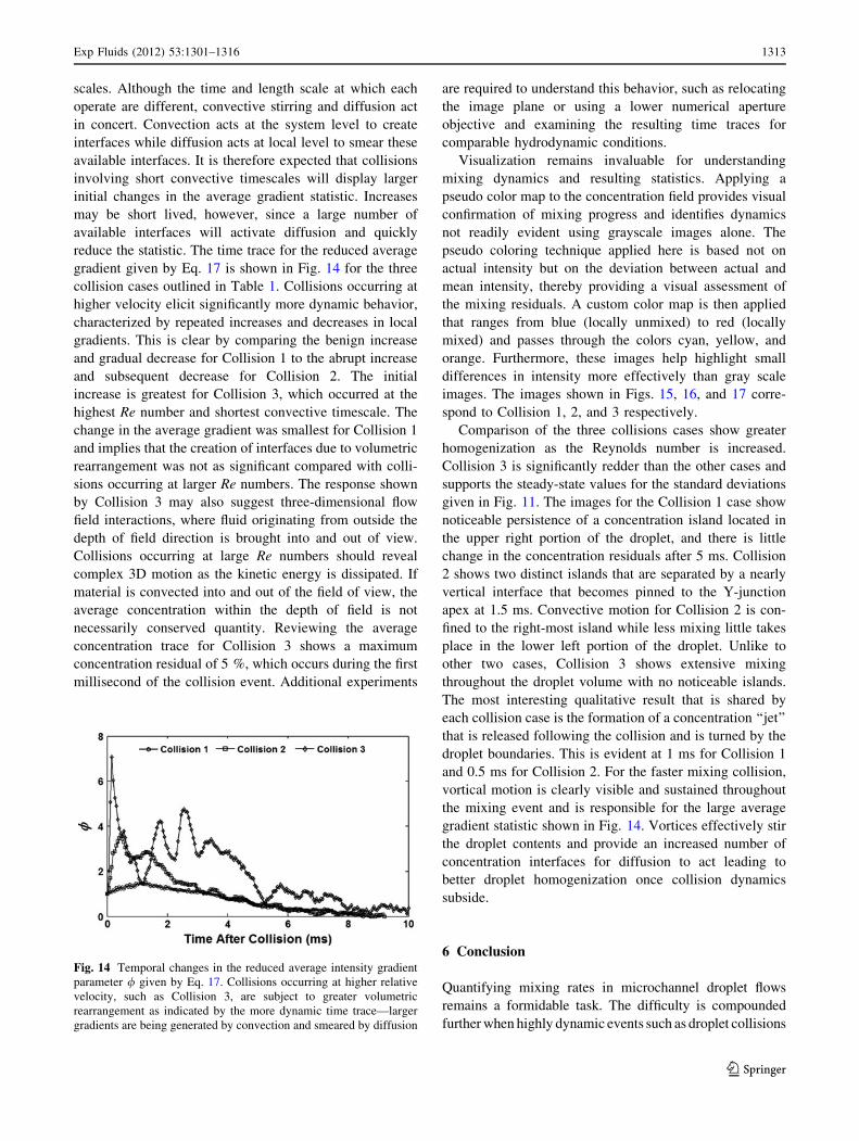
reduce the statistic. The time trace for the reduced average
gradient given by Eq. 17 is shown in Fig. 14 for the three
collision cases outlined in Table 1. Collisions occurring at
higher velocity elicit significantly more dynamic behavior,
characterized by repeated increases and decreases in local
gradients. This is clear by comparing the benign increase
and gradual decrease for Collision 1 to the abrupt increase
and subsequent decrease for Collision 2. The initial
increase is greatest for Collision 3, which occurred at the
highest Re number and shortest convective timescale. The
change in the average gradient was smallest for Collision 1
and implies that the creation of interfaces due to volumetric
rearrangement was not as significant compared with colli-
sions occurring at larger Re numbers. The response shown
by Collision 3 may also suggest three-dimensional flow
field interactions, where fluid originating from outside the
depth of field direction is brought into and out of view.
Collisions occurring at large Re numbers should reveal
complex 3D motion as the kinetic energy is dissipated. If
material is convected into and out of the field of view, the
average concentration within the depth of field is not
necessarily conserved quantity. Reviewing the average
concentration trace for Collision 3 shows a maximum
concentration residual of 5 %, which occurs during the first
millisecond of the collision event. Additional experiments
are required to understand this behavior, such as relocating
the image plane or using a lower numerical aperture
objective and examining the resulting time traces for
comparable hydrodynamic conditions.
Visualization remains invaluable for understanding
mixing dynamics and resulting statistics. Applying a
pseudo color map to the concentration field provides visual
confirmation of mixing progress and identifies dynamics
not readily evident using grayscale images alone. The
pseudo coloring technique applied here is based not on
actual intensity but on the deviation between actual and
mean intensity, thereby providing a visual assessment of
the mixing residuals. A custom color map is then applied
that ranges from blue (locally unmixed) to red (locally
mixed) and passes through the colors cyan, yellow, and
orange. Furthermore, these images help highlight small
differences in intensity more effectively than gray scale
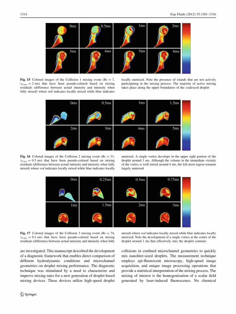
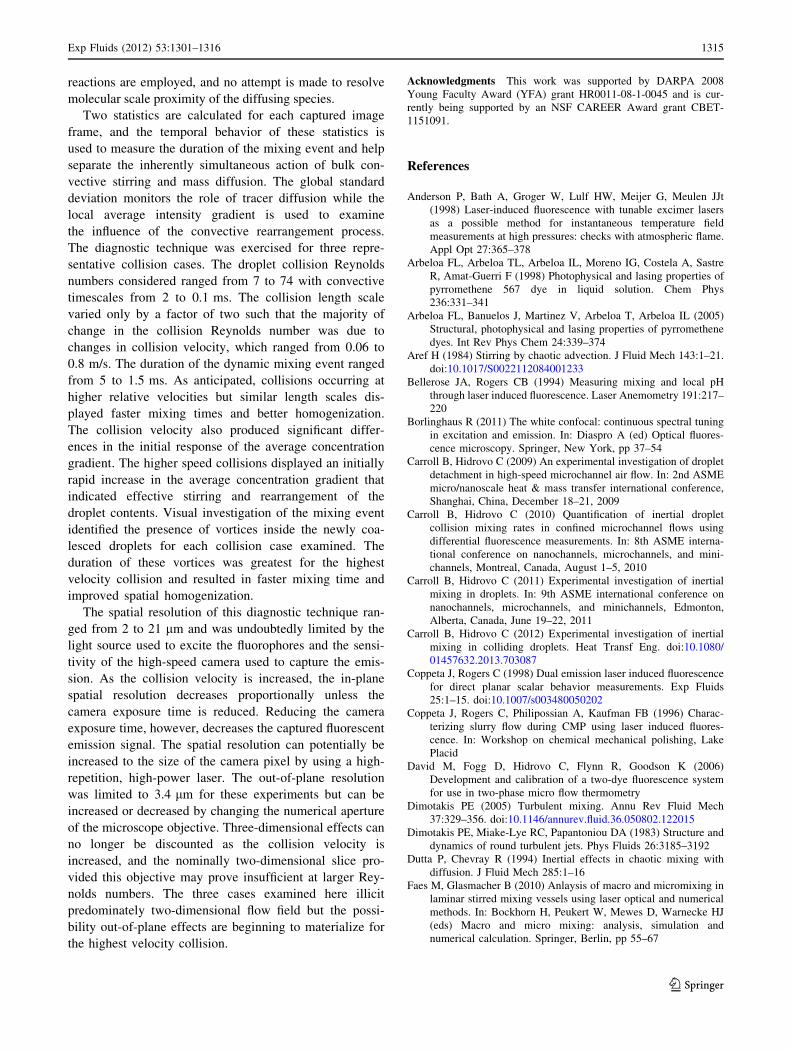
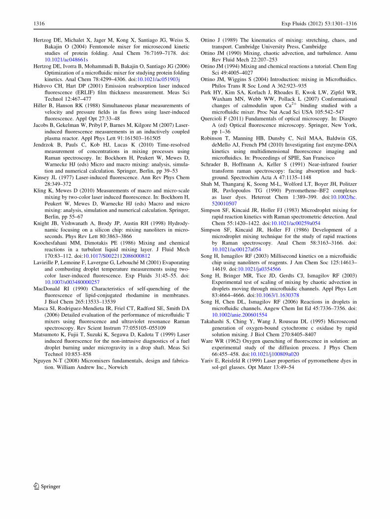
images. The images shown in Figs. 15, 16, and 17 corre-
spond to Collision 1, 2, and 3 respectively.
Comparison of the three collisions cases show greater
homogenization as the Reynolds number is increased.
Collision 3 is significantly redder than the other cases and
supports the steady-state values for the standard deviations
given in Fig. 11. The images for the Collision 1 case show
noticeable persistence of a concentration island located in
the upper right portion of the droplet, and there is little
change in the concentration residuals after 5 ms. Collision
2 shows two distinct islands that are separated by a nearly
vertical interface that becomes pinned to the Y-junction
apex at 1.5 ms. Convective motion for Collision 2 is con-
fined to the right-most island while less mixing little takes
place in the lower left portion of the droplet. Unlike to
other two cases, Collision 3 shows extensive mixing
throughout the droplet volume with no noticeable islands.
The most interesting qualitative result that is shared by
each collision case is the formation of a concentration ‘‘jet’’
that is released following the collision and is turned by the
droplet boundaries. This is evident at 1 ms for Collision 1
and 0.5 ms for Collision 2. For the faster mixing collision,
vortical motion is clearly visible and sustained throughout
the mixing event and is responsible for the large average
gradient statistic shown in Fig. 14. Vortices effectively stir
the droplet contents and provide an increased number of
concentration interfaces for diffusion to act leading to
better droplet homogenization once collision dynamics
subside.
6 Conclusion
Quantifying mixing rates in microchannel droplet flows
remains a formidable task. The difficulty is compounded
further when highly dynamic events such as droplet collisions
Fig. 14 Temporal changes in the reduced average intensity gradient
parameter / given by Eq. 17. Collisions occurring at higher relative
velocity, such as Collision 3, are subject to greater volumetric
rearrangement as indicated by the more dynamic time trace—larger
gradients are being generated by convection and smeared by diffusion
Exp Fluids (2012) 53:1301–1316 1313
123
are investigated. This manuscript described the development
of a diagnostic framework that enables direct comparison of
different hydrodynamic conditions and microchannel
geometries on droplet mixing performance. The diagnostic
technique was stimulated by a need to characterize and
improve mixing rates for a new generation of droplet-based
mixing devices. These devices utilize high-speed droplet
collisions in confined microchannel geometries to quickly
mix nanoliter-sized droplets. The measurement technique
employs epi-fluorescent microscopy, high-speed image
acquisition, and unique image processing operations that
provide a statistical interpretation of the mixing process. The
mixing of interest is the homogenization of a scalar field
generated by laser-induced fluorescence. No chemical
0ms 0.5ms 1ms 2ms
3ms 4ms 5ms 6ms
Fig. 15 Colored images of the Collision 1 mixing event (Re = 7,
sConv = 2 ms) that have been pseudo-colored based on mixing
residuals (difference between actual intensity and intensity when
fully mixed) where red indicates locally mixed while blue indicates
locally unmixed. Note the presence of islands that are not actively
participating in the mixing process. The majority of active mixing
takes place along the upper boundaries of the coalesced droplet
0ms 0.5ms 1ms 1.5ms
2ms 3ms 4ms 5ms
Fig. 16 Colored images of the Collision 2 mixing event (Re = 31,
sConv = 0.5 ms) that have been pseudo-colored based on mixing
residuals (difference between actual intensity and intensity when fully
mixed) where red indicates locally mixed while blue indicates locally
unmixed. A single vortex develops in the upper right portion of the
droplet around 1 ms. Although the volume in the immediate vicinity
of the vortex is well stirred around 4 ms, the left-most region remains
largely unmixed
0ms 0.25ms 0.5ms 0.75ms
1ms 1.5ms 2ms 3ms
Fig. 17 Colored images of the Collision 3 mixing event (Re = 74,
sConv = 0.1 ms) that have been pseudo-colored based on mixing
residuals (difference between actual intensity and intensity when fully
mixed) where red indicates locally mixed while blue indicates locally
unmixed. Note the development of a single vortex at the center of the
droplet around 1 ms that effectively stirs the droplet contents
1314 Exp Fluids (2012) 53:1301–1316
123
reactions are employed, and no attempt is made to resolve
molecular scale proximity of the diffusing species.
Two statistics are calculated for each captured image
frame, and the temporal behavior of these statistics is
used to measure the duration of the mixing event and help
separate the inherently simultaneous action of bulk con-
vective stirring and mass diffusion. The global standard
deviation monitors the role of tracer diffusion while the
local average intensity gradient is used to examine
the influence of the convective rearrangement process.
The diagnostic technique was exercised for three repre-
sentative collision cases. The droplet collision Reynolds
numbers considered ranged from 7 to 74 with convective
timescales from 2 to 0.1 ms. The collision length scale
varied only by a factor of two such that the majority of
change in the collision Reynolds number was due to
changes in collision velocity, which ranged from 0.06 to
0.8 m/s. The duration of the dynamic mixing event ranged
from 5 to 1.5 ms. As anticipated, collisions occurring at
higher relative velocities but similar length scales dis-
played faster mixing times and better homogenization.
The collision velocity also produced significant differ-
ences in the initial response of the average concentration
gradient. The higher speed collisions displayed an initially
rapid increase in the average concentration gradient that
indicated effective stirring and rearrangement of the
droplet contents. Visual investigation of the mixing event
identified the presence of vortices inside the newly coa-
lesced droplets for each collision case examined. The
duration of these vortices was greatest for the highest
velocity collision and resulted in faster mixing time and
improved spatial homogenization.
The spatial resolution of this diagnostic technique ran-
ged from 2 to 21 lm and was undoubtedly limited by the
light source used to excite the fluorophores and the sensi-
tivity of the high-speed camera used to capture the emis-
sion. As the collision velocity is increased, the in-plane
spatial resolution decreases proportionally unless the
camera exposure time is reduced. Reducing the camera
exposure time, however, decreases the captured fluorescent
emission signal. The spatial resolution can potentially be
increased to the size of the camera pixel by using a high-
repetition, high-power laser. The out-of-plane resolution
was limited to 3.4 lm for these experiments but can be
increased or decreased by changing the numerical aperture
of the microscope objective. Three-dimensional effects can
no longer be discounted as the collision velocity is
increased, and the nominally two-dimensional slice pro-
vided this objective may prove insufficient at larger Rey-
nolds numbers. The three cases examined here illicit
predominately two-dimensional flow field but the possi-
bility out-of-plane effects are beginning to materialize for
the highest velocity collision.
Acknowledgments This work was supported by DARPA 2008
Young Faculty Award (YFA) grant HR0011-08-1-0045 and is cur-
rently being supported by an NSF CAREER Award grant CBET-
1151091.
References
Anderson P, Bath A, Groger W, Lulf HW, Meijer G, Meulen JJt
(1998) Laser-induced fluorescence with tunable excimer lasers
as a possible method for instantaneous temperature field
measurements at high pressures: checks with atmospheric flame.
Appl Opt 27:365–378
Arbeloa FL, Arbeloa TL, Arbeloa IL, Moreno IG, Costela A, Sastre
R, Amat-Guerri F (1998) Photophysical and lasing properties of
pyrromethene 567 dye in liquid solution. Chem Phys
236:331–341
Arbeloa FL, Banuelos J, Martinez V, Arbeloa T, Arbeloa IL (2005)
Structural, photophysical and lasing properties of pyrromethene
dyes. Int Rev Phys Chem 24:339–374
Aref H (1984) Stirring by chaotic advection. J Fluid Mech 143:1–21.
doi:10.1017/S0022112084001233
Bellerose JA, Rogers CB (1994) Measuring mixing and local pH
through laser induced fluorescence. Laser Anemometry 191:217–
220
Borlinghaus R (2011) The white confocal: continuous spectral tuning
in excitation and emission. In: Diaspro A (ed) Optical fluores-
cence microscopy. Springer, New York, pp 37–54
Carroll B, Hidrovo C (2009) An experimental investigation of droplet
detachment in high-speed microchannel air flow. In: 2nd ASME
micro/nanoscale heat & mass transfer international conference,
Shanghai, China, December 18–21, 2009
Carroll B, Hidrovo C (2010) Quantification of inertial droplet
collision mixing rates in confined microchannel flows using
differential fluorescence measurements. In: 8th ASME interna-
tional conference on nanochannels, microchannels, and mini-
channels, Montreal, Canada, August 1–5, 2010
Carroll B, Hidrovo C (2011) Experimental investigation of inertial
mixing in droplets. In: 9th ASME international conference on
nanochannels, microchannels, and minichannels, Edmonton,
Alberta, Canada, June 19–22, 2011
Carroll B, Hidrovo C (2012) Experimental investigation of inertial
mixing in colliding droplets. Heat Transf Eng. doi:10.1080/
01457632.2013.703087
Coppeta J, Rogers C (1998) Dual emission laser induced fluorescence
for direct planar scalar behavior measurements. Exp Fluids
25:1–15. doi:10.1007/s003480050202
Coppeta J, Rogers C, Philipossian A, Kaufman FB (1996) Charac-
terizing slurry flow during CMP using laser induced fluores-
cence. In: Workshop on chemical mechanical polishing, Lake
Placid
David M, Fogg D, Hidrovo C, Flynn R, Goodson K (2006)
Development and calibration of a two-dye fluorescence system
for use in two-phase micro flow thermometry
Dimotakis PE (2005) Turbulent mixing. Annu Rev Fluid Mech
37:329–356. doi:10.1146/annurev.fluid.36.050802.122015
Dimotakis PE, Miake-Lye RC, Papantoniou DA (1983) Structure and
dynamics of round turbulent jets. Phys Fluids 26:3185–3192
Dutta P, Chevray R (1994) Inertial effects in chaotic mixing with
diffusion. J Fluid Mech 285:1–16
Faes M, Glasmacher B (2010) Anlaysis of macro and micromixing in
laminar stirred mixing vessels using laser optical and numerical
methods. In: Bockhorn H, Peukert W, Mewes D, Warnecke HJ
(eds) Macro and micro mixing: analysis, simulation and
numerical calculation. Springer, Berlin, pp 55–67
Exp Fluids (2012) 53:1301–1316 1315
123
Hertzog DE, Michalet X, Jager M, Kong X, Santiago JG, Weiss S,
Bakajin O (2004) Femtomole mixer for microsecond kinetic
studies of protein folding. Anal Chem 76:7169–7178. doi:
10.1021/ac048661s
Hertzog DE, Ivorra B, Mohammadi B, Bakajin O, Santiago JG (2006)
Optimization of a microfluidic mixer for studying protein folding
kinetics. Anal Chem 78:4299–4306. doi:10.1021/ac051903j
Hidrovo CH, Hart DP (2001) Emission reabsorption laser induced
fluorescence (ERLIF) film thickness measurement. Meas Sci
Technol 12:467–477
Hiller B, Hanson RK (1988) Simultaneous planar measurements of
velocity and pressure fields in fas flows using laser-induced
fluorescence. Appl Opt 27:33–48
Jacobs B, Gekelman W, Pribyl P, Barnes M, Kilgore M (2007) Laser-
induced fluorescence measurements in an inductively coupled
plasma reactor. Appl Phys Lett 91:161503–161505
Jendrzok B, Pauls C, Kob HJ, Lucas K (2010) Time-resolved
measurement of concentrations in mixing processes using
Raman spectroscopy. In: Bockhorn H, Peukert W, Mewes D,
Warnecke HJ (eds) Micro and macro mixing: analysis, simula-
tion and numerical calculation. Springer, Berlin, pp 39–53
Kinsey JL (1977) Laser-induced fluorescence. Ann Rev Phys Chem
28:349–372
Kling K, Mewes D (2010) Measurements of macro and micro-scale
mixing by two-color laser induced fluorescence. In: Bockhorn H,
Peukert W, Mewes D, Warnecke HJ (eds) Macro and micro
mixing: analysis, simulation and numerical calculation. Springer,
Berlin, pp 55–67
Knight JB, Vishwanath A, Brody JP, Austin RH (1998) Hydrody-
namic focusing on a silicon chip: mixing nanoliters in micro-
seconds. Phys Rev Lett 80:3863–3866
Koochesfahani MM, Dimotakis PE (1986) Mixing and chemical
reactions in a turbulent liquid mixing layer. J Fluid Mech
170:83–112. doi:10.1017/S0022112086000812
Lavieille P, Lemoine F, Lavergne G, Lebouche M (2001) Evaporating
and combusting droplet temperature measurements using two-
color laser-induced fluorescence. Exp Fluids 31:45–55. doi:
10.1007/s003480000257
MacDonald RI (1990) Characteristics of self-quenching of the
fluorescence of lipid-conjugated rhodamine in membranes.
J Biol Chem 265:13533–13539
Masca SI, Rodriguez-Mendieta IR, Friel CT, Radford SE, Smith DA
(2006) Detailed evaluation of the performance of microfluidic T
mixers using fluorescence and ultraviolet resonance Raman
spectroscopy. Rev Scient Instrum 77:055105–055109
Matsumoto K, Fujii T, Suzuki K, Segawa D, Kadota T (1999) Laser
induced fluorescence for the non-intrusive diagnostics of a fuel
droplet burning under microgravity in a drop shaft. Meas Sci
Technol 10:853–858
Nguyen N-T (2008) Micromixers fundamentals, design and fabrica-
tion. William Andrew Inc., Norwich
Ottino J (1989) The kinematics of mixing: stretching, chaos, and
transport. Cambridge University Press, Cambridge
Ottino JM (1990) Mixing, chaotic advection, and turbulence. Annu
Rev Fluid Mech 22:207–253
Ottino JM (1994) Mixing and chemical reactions a tutorial. Chem Eng
Sci 49:4005–4027
Ottino JM, Wiggins S (2004) Introduction: mixing in Microfluidics.
Philos Trans R Soc Lond A 362:923–935
Park HY, Kim SA, Korlach J, Rhoades E, Kwok LW, Zipfel WR,
Waxham MN, Webb WW, Pollack L (2007) Conformational
changes of calmodulin upon Ca2? binding studied with a
microfluidic mixer. Proc Nat Acad Sci USA 105:542–547
Quercioli F (2011) Fundamentals of optical microscopy. In: Diaspro
A (ed) Optical fluorescence microscopy. Springer, New York,
pp 1–36
Robinson T, Manning HB, Dunsby C, Neil MAA, Baldwin GS,
deMello AJ, French PM (2010) Investigating fast enzyme-DNA
kinetics using multidimensional fluorescence imaging and
microfluidics. In: Proceedings of SPIE, San Francisco
Schrader B, Hoffmann A, Keller S (1991) Near-infrared fourier
transform raman spectroscopy: facing absorption and back-
ground. Spectrochim Acta A 47:1135–1148
Shah M, Thangaraj K, Soong M-L, Wolford LT, Boyer JH, Politzer
IR, Pavlopoulos TG (1990) Pyrromethene–BF2 complexes
as laser dyes. Heteroat Chem 1:389–399. doi:10.1002/hc.
520010507
Simpson SF, Kincaid JR, Holler FJ (1983) Microdroplet mixing for
rapid reaction kinetics with Raman spectrometric detection. Anal
Chem 55:1420–1422. doi:10.1021/ac00259a054
Simpson SF, Kincaid JR, Holler FJ (1986) Development of a
microdroplet mixing technique for the study of rapid reactions
by Raman spectroscopy. Anal Chem 58:3163–3166. doi:
10.1021/ac00127a054
Song H, Ismagilov RF (2003) Millisecond kinetics on a microfluidic
chip using nanoliters of reagents. J Am Chem Soc 125:14613–
14619. doi:10.1021/ja0354566
Song H, Bringer MR, Tice JD, Gerdts CJ, Ismagilov RF (2003)
Experimental test of scaling of mixing by chaotic advection in
droplets moving through microfluidic channels. Appl Phys Lett
83:4664–4666. doi:10.1063/1.1630378
Song H, Chen DL, Ismagilov RF (2006) Reactions in droplets in
microfluidic channels. Angew Chem Int Ed 45:7336–7356. doi:
10.1002/anie.200601554
Takahashi S, Ching Y, Wang J, Rouseau DL (1995) Microsecond
generation of oxygen-bound cytochrome c oxidase by rapid
solution mixing. J Biol Chem 270:8405–8407
Ware WR (1962) Oxygen quenching of fluorescence in solution: an
experimental study of the diffusion process. J Phys Chem
66:455–458. doi:10.1021/j100809a020
Yariv E, Reisfeld R (1999) Laser properties of pyrromethene dyes in
sol-gel glasses. Opt Mater 13:49–54
1316 Exp Fluids (2012) 53:1301–1316
123