dry bulk shipping and business cycles
TRANSCRIPT
Norges Handelshøyskole
Bergen, Spring 2010
Master Thesis within the main profile of Financial Economics
Thesis Advisor: Professor Siri Pettersen Strandenes
Dry bulk shipping andbusiness cycles
Ivar Sandvig Thorsen
This thesis was written as a part of the masterprogram at NHH. Neither
the institution, the advisor, nor the sensors are - through the approval of
this thesis - responsible for neither the theories and methods used, nor
results and conclusions drawn in this work.


1
Abstract
This thesis studies short- and long-term relationships between
freight rates in dry bulk shipping and business cycles. The analysis
combines a theoretical specification of the market with an econo-
metric approach to study time series data. In the empirical part of
the thesis several of the business cycle indicators, including the gdp
for all of the countries tested, turned out to be cointegrated with
the freight rates. This result means that there exists an equilibrium
relationship between the business cycle and the freight rates in dry
bulk shipping. Error correction models were then used to study the
short-term dynamics between the cointegrated freight rates and the
relevant business cycle measures. The thesis further illustrates the
importance of interpreting the empirical results in terms of a com-
petitive equilibrium model.
2
Foreword
Since I was young I have had a genuine interest in shipping. Therefore, I
am very grateful for the unique opportunity working with this thesis has
given me to learn more about the shipping industry.
First and foremost, I would like to thank my thesis advisor Professor
Siri Pettersen Strandenes. It has been very inspiring and instructive to
have an advisor with such a unique insight to the shipping industry. In
addition to my thesis advisor, I would also like to thank Associate Profes-
sor Jonas Anderson at NHH for helpful comments on the econometric part
of my thesis. Finally, I am grateful to my father, Inge Thorsen, who has
contributed with valuable comments and ideas to the theoretical part of
this thesis, and to Arnstein Gjestland at the Stord/Haugesund University
College for technical assistance on the use of LaTeX.
Ivar Sandvig Thorsen1
Bergen, June 2010
1Norwegian School of Economics and Business Administration, Helleveien 30, N-5045Bergen, Norway. e-mail: [email protected]
Contents
Abstract 1
Foreword 2
Contents 3
1 Introduction 5
2 Basic definitions and data 7
2.1 Bulk commodities, vessels and freight rates . . . . . . . . . . 8
2.2 Data sources . . . . . . . . . . . . . . . . . . . . . . . . . . . 13
3 Modeling markets for dry bulk shipping. A literature
review. 14
3.1 Competitive and integrated markets . . . . . . . . . . . . . . 16
3.2 The supply of shipping services . . . . . . . . . . . . . . . . 18
3.3 The demand for shipping services . . . . . . . . . . . . . . . 22
3.4 Shipping market equilibrium . . . . . . . . . . . . . . . . . . 26
4 Observed variations in shipping volumes and freight rates 26
5 Some basic issues in time series analyses 29
5.1 Stationarity and spurious regression . . . . . . . . . . . . . . 29
5.2 Cointegration . . . . . . . . . . . . . . . . . . . . . . . . . . 32
5.3 The error correction model . . . . . . . . . . . . . . . . . . . 34
6 Short- and long-term relationships between freight rates
and business cycle measures 36
6.1 Testing based on quarterly data . . . . . . . . . . . . . . . . 37
6.1.1 Stationarity of freight rates and some business cycle
measures . . . . . . . . . . . . . . . . . . . . . . . . . 38
6.1.2 Testing for integration order . . . . . . . . . . . . . . 39
6.1.3 Cointegration . . . . . . . . . . . . . . . . . . . . . . 40
3
4 CONTENTS
6.1.4 Results based on Error Correction Models . . . . . . 42
6.2 Results based on monthly data . . . . . . . . . . . . . . . . 44
6.2.1 Stationarity of freight rates, trade flows and produc-
tion measures . . . . . . . . . . . . . . . . . . . . . . 46
6.2.2 Testing for stationarity of the first differences . . . . 48
6.2.3 Cointegration . . . . . . . . . . . . . . . . . . . . . . 49
6.2.4 Results based on Error Correction Models . . . . . . 50
6.3 Critical remarks on the empirical results . . . . . . . . . . . 53
7 Interpreting results in terms of a competitive equilibrium
model 56
7.1 A general demand shock . . . . . . . . . . . . . . . . . . . . 56
7.2 A demand shock in a separate submarket . . . . . . . . . . . 59
7.3 Effects of an increased price of bunker fuel . . . . . . . . . . 62
7.4 The dramatic recent fall in freight rates . . . . . . . . . . . . 64
8 A summary of results and some concluding remarks 67
Bibliography 72
Appendices 77
A Illustrations of the quarterly time series used in this thesis 79
B Illustrations of the monthly time series used in this thesis 81
C Stata commands 88
5
1 Introduction
The main ambition of this master’s thesis is to study potential short- and
long-term relationships between freight rates in dry bulk shipping and busi-
ness cycles. Shipping is widely known to be a highly volatile industry. Un-
derstanding and predicting this volatility is important for participants of
the industry, in making operating and investment decisions. In this thesis
the dynamics of the dry bulk shipping market is explained by combining an
econometric approach to study time series data with a theoretical analysis
of the market. The thesis focuses primarily on the impact of alternative
business cycle measures as possible determinants of the volatility.
As for the analysis of most markets, there is ambiguity in defining vari-
ables representing price and volume. There are for instance different freight
rates depending on factors such as the fixture, route and cargo. In this the-
sis, however, I will be using the Baltic Freight Index (BFI) as a measure of
the freight rates in dry bulk shipping. It is also challenging to find accurate
measures of business cycles, representing the demand for shipping services.
I will be using quarterly data on gdp for OECD, USA, Japan and China as
measures of business cycles. In addition to this, I will study monthly data
on industrial production and steel production, as well as data on trade for
relevant countries/areas.
Freight rates in bulk shipping result from an equilibrium between supply
and demand of transportation of bulk commodities. Several models have
been developed to explain and predict freight rates in shipping. Two ex-
amples are the NORBULK-model developed by Strandenes and Wergeland
(1980), and the Stopford Model (Stopford 2009). The demand for sea trans-
port is derived from the demand for specific commodities, while the supply
is represented by the size and the productivity of the fleet. As mentioned
above, the discussion in this paper is restricted to dry bulk commodities.
According to Stopford (2009, p. 419-421) such commodities are shipped
in large, unpackaged amounts, usually divided into major bulks and mi-
nor bulks. Examples of major dry bulk commodities are coal, iron ore and
grain, while minor bulks include for instance steel, sugar and cement.
6 1. INTRODUCTION
In a short-term time perspective the impact of demand shocks may
sometimes be studied within a framework where the supply of sea transport
is assumed to be inelastic with respect to variation in freight rates. This
can at least be argued to apply in scenarios where the market operates
close to the capacity constraint, involving all available bulk carriers. The
discussion is of course very different in a scenario of recession, with low
capacity utilization in the fleet of bulk carriers.
The time perspective is important also in an evaluation of the supply
side of the market for transporting bulk commodities. It is reasonable to
assume that the size and productivity of the fleet depend on the observed
development of the freight rates in dry bulk shipping, and on expectations
of future demand and future freight rates. One challenge, however, is that
the process between the ordering and the deliveries of new carriers is time
consuming; the market conditions may be substantially changed at the time
when the deliveries are effectuated.
Both the freight rate and the indicators I will be using for business cy-
cles are expected to be non-stationary. It is well known in the literature
that results from times series regressions between non-stationary variables
may reflect spurious relationships. If, however, there is a linear combination
of the two non-stationary series that is stationary, the two series are coin-
tegrated. In such cases there exists a long-term equilibrium between the
two series, and we do not have to worry about spuriousness. We can then
use an Error Correction Model to study the short-run dynamics between
the two series. Hence, the times series used in this thesis will be tested for
stationarity and cointegration. In cases where the series are cointegrated,
I will be using an Error Correction Model to study short-term dynamics
between the freight rates and the indicators of business cycles.
According to theoretical and empirical analysis, the supply of sea trans-
port is highly non-linearly dependent on the freight rates. This contributes
to call for a careful interpretation of econometric results, since the impact of
demand shocks depend on the initial capacity utilization of the fleet. This
is one example why I have emphasized the importance of supplementing
econometric results with a theoretical discussion of the shipping market.
7
The analysis to follow focuses first on possible relationships between
freight rates in dry bulk shipping and business cycles in general. In addition
a more disaggregated approach is employed to study freight rates for dif-
ferent categories of bulk carriers, and for transport between geographically
different markets for imports and exports. One ambition of this analysis is
to test whether the law of one price applies for shipping in such markets.
In theory this law applies in competitive markets, relying for instance on
the assumption of free entry and free exit, and ignoring transport costs of
moving from one submarket to another. Hence, temporary differences in
shipping rates between submarkets may reflect both time lags in adjusting
the size of the fleet, and costs of moving to another market segment. Such
costs may explain persisting differentials in freight rates between submar-
kets.
The thesis starts with a presentation of some basic definitions and data
in Section 2. Based on a literature review, Section 3 provides an introduc-
tion to the supply and demand of sea transport. There is a short presen-
tation of how the key variables in this market have developed over time in
Section 4. Section 5 focuses on the econometric techniques I will be using
in this thesis. Those techniques are then used in Section 6 to study short
and long-term relationships between freight rates in dry bulk shipping and
different measures of business cycles. In Section 7, the empirical results
are interpreted in terms of the partial competitive equilibrium model pre-
sented in Section 3. Finally, a summary of the results and some concluding
remarks are given in Section 8.
2 Basic definitions and data
The goods that are shipped from an origin to a destination are not ho-
mogenous. This does not, however, necessarily mean that shipping services
are heterogeneous; the character and costs of shipping may be more or less
independent of what goods are being transported. Still, different vessels
are to some degree used for transporting different kinds of goods. Despite a
relatively high degree of substitutability between different shipping services,
8 2. BASIC DEFINITIONS AND DATA
it therefore makes sense to categorize both goods and vessels related to the
transportation of dry bulk cargo. In addition, disaggregated information on
the production and export patterns of different goods may prove useful in
interpreting empirical results on the variation in freight rates. It also gives
an opportunity to study the general freight market impact of a demand
shock in a specific market for traded goods.
Besides specifying different kinds of bulk commodities this section offers
a brief description of different vessels for bulk shipping. In addition, both
the empirical and the theoretical analysis call for a precise definition of
freight rates. Finally, a brief presentation is offered of the data sources
used in the empirical sections of the thesis.
2.1 Bulk commodities, vessels and freight
rates
According to Stopford (2009, p. 61) the shipping market is divided in three
major segments. These segments are bulk shipping, specialized shipping
and liner shipping. The focus of this thesis is bulk shipping and so I will
only briefly explain specialized and liner shipping.
Some cargoes can be challenging to transport in standard vessels. There
may be several reasons for this. It may for example be the shape or the size
of the cargo that is not well suited for standard vessels. For these cargoes
shipowners can greatly improve the efficiency of the transportation by in-
vesting in specialized vessels (Stopford, 2009, p. 469). Stopford (2009, p.
469) discusses five major cargo groups that falls under specialized shipping;
liquified gas, refrigerated cargo, chemicals, passenger shipping and unit load
cargoes.
Much of the cargo transported by sea are traded in parcels not large
enough to fill an entire vessel. For this cargo we have liner shipping. Liner
shipping companies operate a fleet that is sailing a regular route between
fixed terminals at set times (Stopford 2009, p. 512). Any cargo owner can
ship their cargo with these vessels at a predictable price. Liner shipping is
2.1. BULK COMMODITIES, VESSELS AND FREIGHT RATES 9
now almost exclusively operated by container vessels.
Commodities traded in cargo loads large enough to fill up a vessel are
transported in bulk. According to Stopford (2009, p. 424-427) the five
principles of bulk transport are efficient cargo handling, minimize cargo
handling, integrating transport modes employed, and to optimize stocks
for the producer and consumer. Bulk shipping can be divided into dry bulk
and tanker. The main cargoes that are shipped in tankers are crude oil
and oil products (Stopford 2009, p. 422). This thesis focuses, however, on
dry bulk cargo. A further distinction can be made between minor bulk and
major bulk:
Minor bulk : agribulks, sugar, fertilizers, metals and minerals, steel prod-
ucts, forest products, bauxite and metal concentrates (see for instance
Stopford (2009, p. 422) and Laulajainen (2006))
Major bulk : iron ore, coal, grain (inclusive soya)
For the discussion in the analytical parts of this thesis it is useful to add
some information on the major bulk commodity trades. The information
offered here is based on Stopford (2009, p. 445 - 466). Iron ore is the
largest of the trades, as the principal raw material of the steel industry.
The size of the ships has increased somewhat over time, corresponding to a
strategy of using large, specially designed ships on a shuttle service between
the mine and the steel plant (Stopford, 2009, p. 446). Australia and Brazil
account for around 70% of iron ore exports, and the suppliers compete for
the markets in Asia and the North-Atlantic. Distance between origins and
destinations has increased, explaining the tendency that larger ships have
been employed over time. According to Stopford (2009, p. 450) 80% was
carried in ships over 80000 dwt by 2005. Stopford explains this tendency
as a result of improvements in port facilities, but also remarks that many
small vessels are continued to being used.
Coal represents a more complex trade, with two very different markets
(Stopford, 2009, p. 450). Cooking coal is used as a raw material of the steel
industry, while thermal coal is used to fuel power stations, in competition
10 2. BASIC DEFINITIONS AND DATA
with oil and gas. According to Stopford (2009, p. 452) Australia provides
more than a third of the exports, while Europe, Japan and other far east
countries are the main importers of coal. Stopford also explains why bulk
carriers used in coal trade on average (109000 dwt) are smaller than those
used in iron ore trade (an average of 148000 dwt). The explanation is related
to volumes to stockpile, value, and the risk of spontaneous combustion in
very large cargoes.
The third major bulk, grain, is an agricultural commodity, and has very
different shipping terms than the two others. Due to a greater demand for
meat consumption at higher income levels, there has been an upward trend
in seaborne grain imports (Stopford, 2009, p. 454). 46% of total exports
is accounted for by the US, while imports are widely spread (Stopford,
2009, p. 455). According to Stopford (2009, p. 455) average trade flows
are relatively small, and the transport system needs to be flexible for this
agricultural crop.
Notice in particular that both coal and iron ore is used as raw materials
of the steel industry. It will turn out to be important in this thesis that
such steel-related transport is a dominating part of dry bulk shipping.
Different cargo are typically shipped in vessels of different size (see for
instance Laulajainen 2006, Table 1.7 and 1.8). The different vessels used
for dry bulk shipping can be categorized as follows (Stopford, 2009, p. xxi
and p. 591) and Laulajainen (2006):
Capesize : the largest bulk carriers. 100,000+. Usually 170,000 - 180,000
dwt
Panamax : the largest bulk carriers that can transit the Panama Canal.
60,000 - 100,000 dwt
Handymax : 40,000 - 60,000 dwt
Handy : 10,000 - 40,000 dwt
Laulajainen (2006) and Stopford (2009, p. 590-592) offer a detailed descrip-
tion of the different kinds of vessels, and explains the demand for different
sizes.
2.1. BULK COMMODITIES, VESSELS AND FREIGHT RATES 11
There are several measures of freight rates, corresponding to different
bulk cargo, specific vessels, particular voyage routes and different kinds of
contracts. According to Laulajainen (2006) freight rates in the Atlantic
might for instance differ systematically from freight rates in the Pacific,
and the rates reflect for instance the likelihood of obtaining backhaul cargo.
The willingness-to-pay for freight services also reflect the price per unit of
the specific cargo. The demand for transport of expensive commodities
tends to be less sensitive to changes in the freight rates than lower priced
commodities.
Hence, it is definitely not possible to identify a single freight rate to
be used in an econometric analysis of shipping markets. Not only does
the freight rates vary depending on the route and the cargo - there are also
several types of fixtures (See Laulajainen (2006, p. 65-67) or Stopford (2009,
p. 182-185). The most common fixtures are Contract of Affreightment
(COA), voyage charter, time charter and bare boat charter (Stopford, 2009,
p. 182-185). The allocation of costs differs between the different fixtures
types. In a voyage charter, the owner pays the voyage cost (i.e. bunkers
and port charges), while in a time charter, the voyage cost is paid by the
charterer (Stopford, 2009, p. 183-185). Hence, the freight rate depends
on the fixture. In theory, the time charter rate is the discounted expected
future spot rate.
According for instance Randers and Goluke (2007) specific freight rates
are strongly correlated over time, in the competitive shipping markets.
Hence, any choice of specification may prove to be adequate in an econo-
metric analysis. Since my analysis is not related to a specific route, bulk
commodity, or vessel, however, an index is chosen to represent freight rates.
The Baltic Freight Index (BFI) was established by the Baltic Exchange
in 1985. It then consisted of 13 voyage routes covering cargoes from 14,000
mt of fertilizer up to 120,000 mt of coal, and no time charter routes.2
Handysizes were removed from the index in 1997, and capesizes in 1999
2For more information, see http://www.balticexchange.com/media/pdf/a%20history%20of%20baltic%20indices%20010610.pdf, that also offers a detailed information of thechanges and amendments that have been introduced since 1985.

12 2. BASIC DEFINITIONS AND DATA
(Laulajainen 2006). The Baltic Exchange Dry Index (BDI) was introduced
in 1999, as an indicator for the dry bulk market and can be used instead
of the Baltic Freight Index, which was discontinued. Kavussanos (2002)
claims that the restructuring over time makes the index a less than ideal
market indicator. In my analysis I have been using the Baltic Freight Index.
Even though the BFI ceased to exist when the Baltic Exchange Dry Index
was introduced, it has been calculated and reported by Clarksons Research
until today.
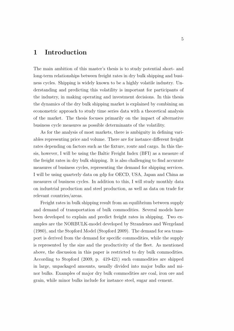
As pointed out both by Randers and Goluke (2007) and Glen and Rogers
(1997), however, the correlation between the different rates make the index
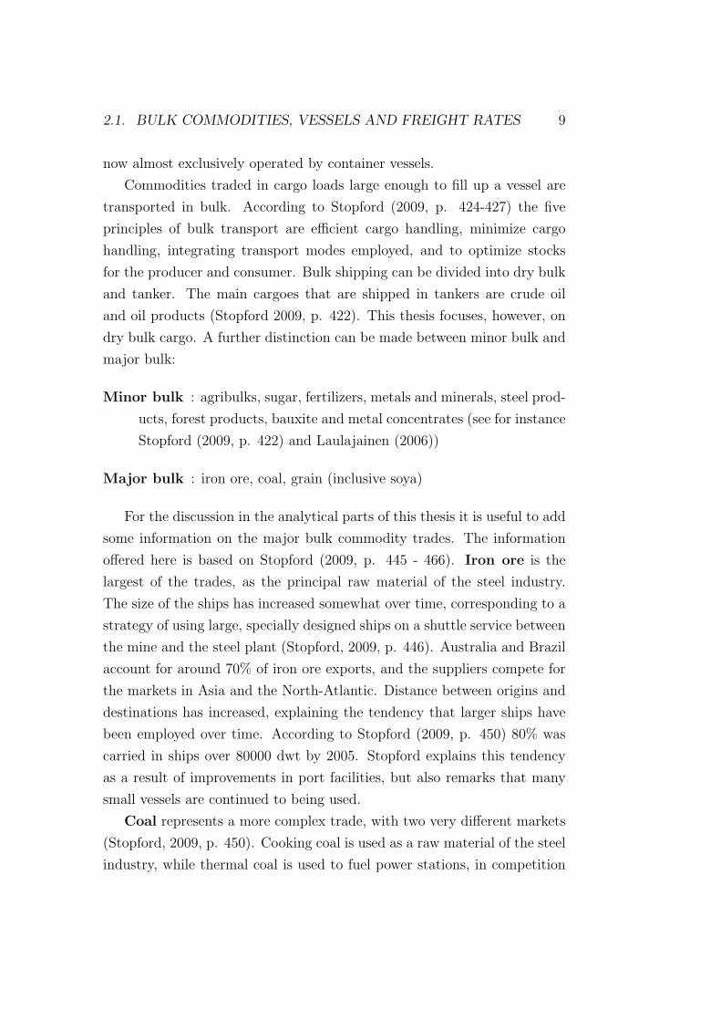
adequately accurate for analytical purposes. Figure 1 illustrates that the
freight rates related to different vessel categories are highly correlated. This
provides an argument that they could all represent the development of
general freight rates in a time series analysis. Notice, however, that despite
the high degree of covariation, there may be substantial differences at a
specific point in time, as pointed out by Laulajainen (2006).
The representativeness of the indices further has to be evaluated from
the fact that the Baltic Exchange handles 30-40% of global dry bulk char-
tering (Shelley 2003), and that the Baltic Exchange Dry Index (BDI) is
made up of 20 key dry bulk routes.3
The Baltic indices are reported on a daily basis. For most of the variables
to be introduced in the empirical analysis in Section 6, however, information
is only available on a monthly or quarterly basis. To match this information,
data on freight rates are converted into monthly and quarterly observations
by calculating the averages of daily observations. As a result freight rates
may seem less volatile than they would if the time series referred to one
specific date each month.
3www.balticexchange.com
2.2. DATA SOURCES 13
00
010010
0100200
200
20030030
0300400
400
4001998m1
1998m1
1998m12000m1
2000m1
2000m12002m1
2002m1
2002m12004m1
2004m1
2004m12006m1
2006m1
2006m12008m1
2008m1
2008m12010m1
2010m1
2010m1time
time
timeBaltic Freight Index rebased
Baltic Freight Index rebased
Baltic Freight Index rebasedBaltic Panamax Index rebased
Baltic Panamax Index rebased
Baltic Panamax Index rebasedBaltic Capesize Index rebased
Baltic Capesize Index rebased
Baltic Capesize Index rebasedBaltic Handysize Index rebased
Baltic Handysize Index rebased
Baltic Handysize Index rebasedBaltic Supramax Index (Handymax) rebased
Baltic Supramax Index (Handymax) rebased
Baltic Supramax Index (Handymax) rebased
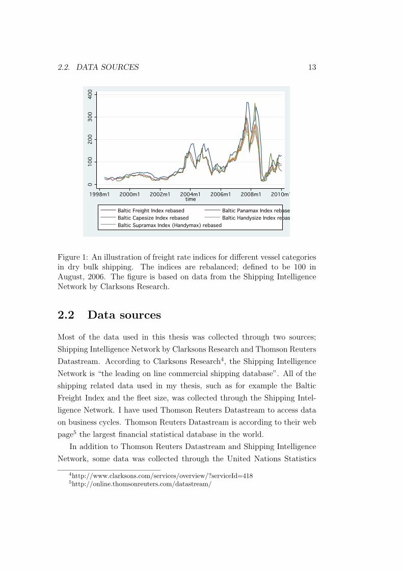
Figure 1: An illustration of freight rate indices for different vessel categoriesin dry bulk shipping. The indices are rebalanced; defined to be 100 inAugust, 2006. The figure is based on data from the Shipping IntelligenceNetwork by Clarksons Research.
2.2 Data sources
Most of the data used in this thesis was collected through two sources;
Shipping Intelligence Network by Clarksons Research and Thomson Reuters
Datastream. According to Clarksons Research4, the Shipping Intelligence
Network is “the leading on line commercial shipping database”. All of the
shipping related data used in my thesis, such as for example the Baltic
Freight Index and the fleet size, was collected through the Shipping Intel-
ligence Network. I have used Thomson Reuters Datastream to access data
on business cycles. Thomson Reuters Datastream is according to their web
page5 the largest financial statistical database in the world.
In addition to Thomson Reuters Datastream and Shipping Intelligence
Network, some data was collected through the United Nations Statistics
4http://www.clarksons.com/services/overview/?serviceId=4185http://online.thomsonreuters.com/datastream/
143. MODELING MARKETS FOR DRY BULK SHIPPING. A
LITERATURE REVIEW.
Division 6 and OECD.stat 7.
3 Modeling markets for dry bulk shipping.
A literature review.
The freight rates in dry bulk shipping is a result of the demand and the
supply of transportation of bulk commodities. The demand and supply
of transportation is derived from a geographical imbalance between the
production and the processing and consumption of commodities. Hence,
the geographically dispersed distribution of resources, consumers, and pro-
cessing industry introduces an important geographical dimension into the
analysis of shipping markets. According to Laulajainen (2006, p. 6) “At-
lantic and Pacific are the main operational theaters and the Atlantic is the
larger of the two. That was back in 1997. Today, China’s economic growth
may have turned the scales in Pacific’s favor. ... The Atlantic and Pacific
Spheres have much interaction in cargo, compared to their internal flows.
The interaction is not balanced however, and the flows from the Atlantic
are in each size segment roughly twice of the opposing flows”.
The supply and demand for sea transport is measured in ton miles, which
is defined as average haul multiplied by tonnage of cargo (Strandenes and
Wergeland, 1980). Several models have been developed to explain and pre-
dict shipping freight rates by studying the factors that influence the demand
and the supply for the corresponding services. According to Beenstock and
Vergottis (1993, p. 72), one of the earliest econometric applications was
Tinbergen (1934). Since then, new models have been developed. The basic
ideas are similar, but the models have become more sophisticated as new
econometric techniques have been developed. One important contribution
to explain and predict freight rates in dry bulk shipping was NORBULK,
a model that was developed and presented in Strandenes and Wergeland
(1980).
6http://unstats.un.org7http://oberon.sourceoecd.org/vl=6310340/cl=19/nw=1/rpsv/dotstat.htm

15
!"#$%&'()$*"%"+,*)
-$.$("/+$%#)
0$.$()"1)$*"%"+,*)'*&.,#2)
3$+'%-)1"4)-42)56(7)*"++"-,&$8)9,((:);"%%$8)/$4)2$'4)
3$+'%-)1"4)-42)56(7)#4'%8/"4#'&"%)
<,((,"%)#"%%$=+,($8)/$4)2$'4)
>6//(2)"1)-42)56(7)#4'%8/"4#'&"%)<,((,"%)#"%%$=+,($8)/$4)2$'4)
?$'()/4,*$)"1)56%7$4)",()
!"#$%&'()@$$#)9,((:)-A#)
342)56(7)8/"#)14$,BC#)
4'#$)
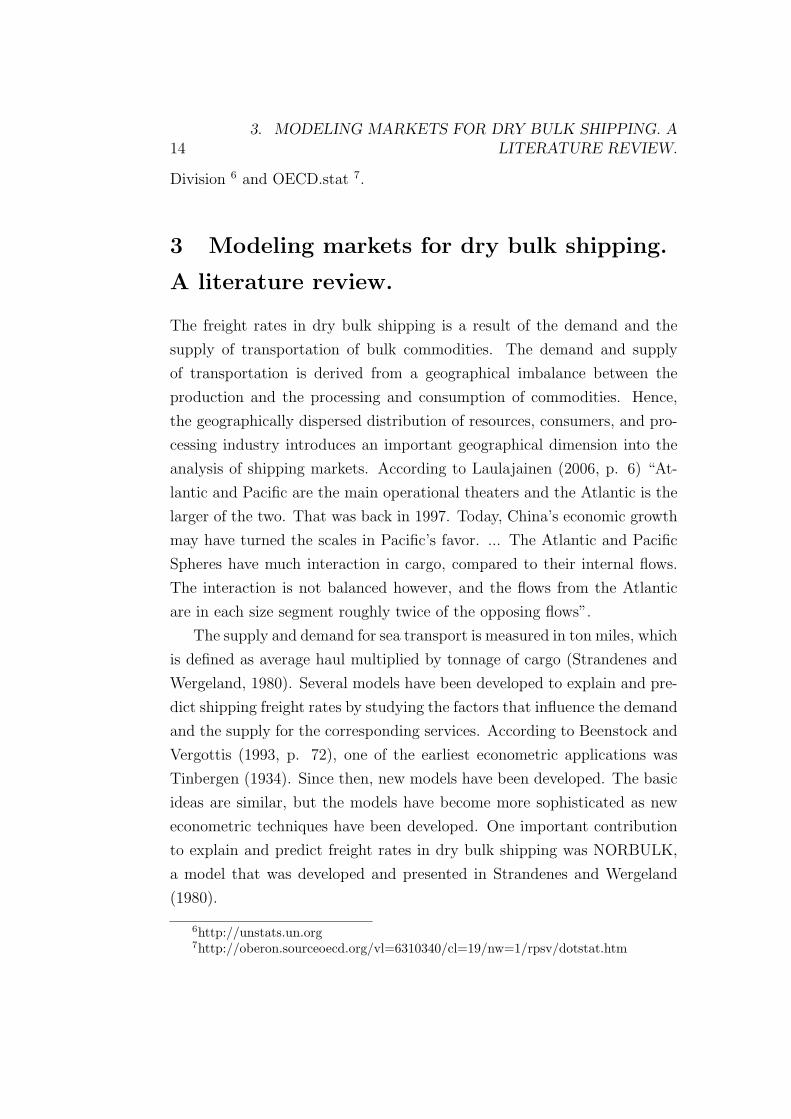
Figure 2: An illustration of the NORBULK model. Source: Strandenes andWergeland (1980)
163. MODELING MARKETS FOR DRY BULK SHIPPING. A
LITERATURE REVIEW.
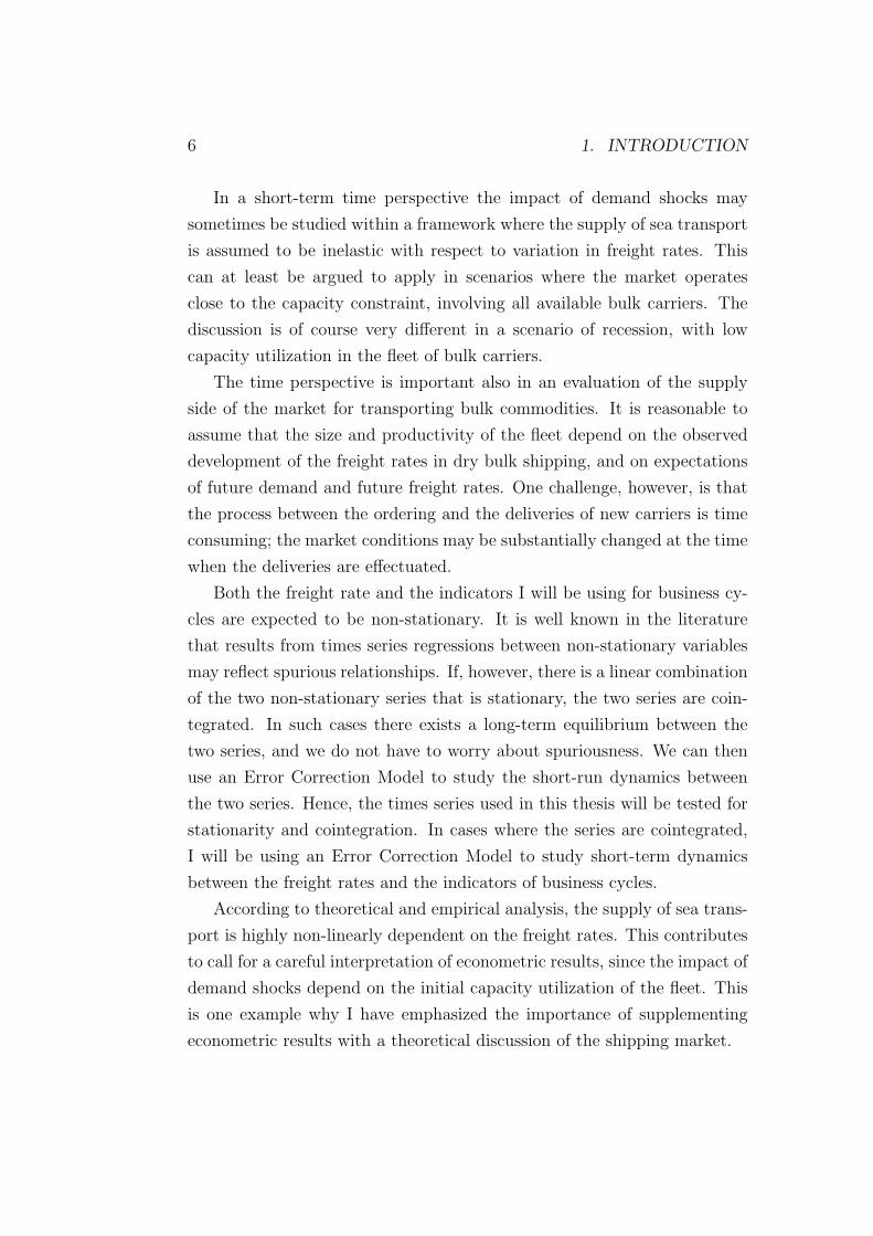
A graphical illustration of the NORBULK model is offered in Figure
2. It follows from this illustration that the demand and the supply of
shipping services are assumed to be influenced by the freight rates. At
the same time the equilibrium freight rates reflect the demand and the
supply of shipping services. The model also accounts for the fact that
macroeconomic conditions (the production capacity and the business cycle
situation) influence the trade of bulk commodities, which further affects the
demand for transportation of dry bulk commodities. The specification of the
relationship between trade and the aggregated macroeconomic condition is
a distinct feature of the NORBULK model. Most other models are focussing
on the major bulk commodities, separately. Finally, it also appears from
Figure 2 that the supply of shipping services is assumed to reflect the size
of the fleet, the fuel price, and the freight rate.
Similar models can also be found in more recent literature, like for ex-
ample Stopford (2009). The basic elements are the same in the alternative
model formulations. The model formulations are made within the frame-
work of a competitive market equilibrium, focussing on the determinants of
supply and demand in the market for dry bulk shipping. This section will
go into more details on such elements, to prepare for an interpretation of
the empirical results to be presented in subsequent sections.
3.1 Competitive and integrated markets
It is often claimed in the literature that the freight markets in bulk shipping
serve as examples of perfectly competitive markets, see for instance Nor-
man (1979), Fuglseth and Strandenes (1997), Koekebakker et al. (2006),
Adland and Strandenes (2004), and Stopford (2009). The market has a high
number of small actors, that individually have only marginal impact on the
market price (freight rates). Market information is readily available, and
“the vibrant market for second-hand ships is said to manifest the relative
ease of overall entry and exit” (Laulajainen 2006, p. 2).
The assumption of homogeneous goods/services is not fulfilled, however.
Due to the geographical dimension, reflecting a dispersed distribution of re-
3.1. COMPETITIVE AND INTEGRATED MARKETS 17
sources and demand for the goods, there exist different routes with different
cargos and specific freight rates. Hence, the bulk shipping market can be
specified into different submarkets, distinguishing between routes, carriers,
and cargo, and “it is generally accepted that freight markets in bulk ship-
ping are examples of almost perfectively competitive markets” (Fuglseth
and Strandenes 1997).
In the empirical part of this thesis, however, I consider the market for
bulk shipping in general, based on a price index and data of freight flows that
are aggregated over all the submarkets. There is a relatively high degree
of competitiveness and substitutability between routes, carriers, and cargo,
forcing a close connection and interaction between different submarkets.
Based on data from the 1960s and 1970s Strandenes (1981) argues that
shocks in one submarket spreads to other submarkets, and that the freight
market in general can be considered to be integrated. This is for instance
reflected by the strongly correlated freight rates over time, see Section 2.1
and Figure 1 above.
There are of course limits to substitution and integration, see for in-
stance Glen (1990) and Adland and Strandenes (2004). Adland and Stran-
denes (2004) consider the market for Very Large Crude Carriers (VLCCs),
modeled as a separate market from the rest of the tanker market. Despite
the correlation due to the potential for substitution, they claim that there
will exist a positive freight rate differential between e.g. a Suezmax tanker
and a VLCC trading on the same route. This differential is explained to
result from the economies of scale offered by the VLCC.
It is evident that different vessels cannot always substitute each other,
and that differences should be expected between freight rates in specific
submarkets. Still, I think that it makes good sense to do analyses based
on aggregated models of dry bulk shipping. As stated in Strandenes and
Wergeland (1980) there are some advantages of aggregating over separate
submarkets, focusing on basic economic relationships rather than getting
lost in the specification of a large number of details on submarkets.
183. MODELING MARKETS FOR DRY BULK SHIPPING. A
LITERATURE REVIEW.
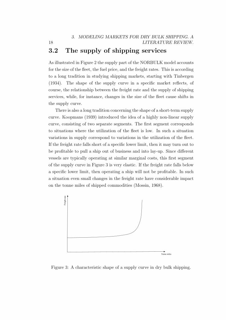
3.2 The supply of shipping services
As illustrated in Figure 2 the supply part of the NORBULK model accounts
for the size of the fleet, the fuel price, and the freight rates. This is according
to a long tradition in studying shipping markets, starting with Tinbergen
(1934). The shape of the supply curve in a specific market reflects, of
course, the relationship between the freight rate and the supply of shipping
services, while, for instance, changes in the size of the fleet cause shifts in
the supply curve.
There is also a long tradition concerning the shape of a short-term supply
curve. Koopmans (1939) introduced the idea of a highly non-linear supply
curve, consisting of two separate segments. The first segment corresponds
to situations where the utilization of the fleet is low. In such a situation
variations in supply correspond to variations in the utilization of the fleet.
If the freight rate falls short of a specific lower limit, then it may turn out to
be profitable to pull a ship out of business and into lay-up. Since different
vessels are typically operating at similar marginal costs, this first segment
of the supply curve in Figure 3 is very elastic. If the freight rate falls below
a specific lower limit, then operating a ship will not be profitable. In such
a situation even small changes in the freight rate have considerable impact
on the tonne miles of shipped commodities (Mossin, 1968).
Fre
ight
rate
Tonne miles
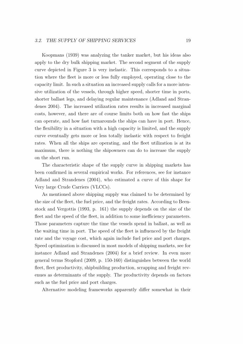
Figure 3: A characteristic shape of a supply curve in dry bulk shipping.
3.2. THE SUPPLY OF SHIPPING SERVICES 19
Koopmans (1939) was analyzing the tanker market, but his ideas also
apply to the dry bulk shipping market. The second segment of the supply
curve depicted in Figure 3 is very inelastic. This corresponds to a situa-
tion where the fleet is more or less fully employed, operating close to the
capacity limit. In such a situation an increased supply calls for a more inten-
sive utilization of the vessels, through higher speed, shorter time in ports,
shorter ballast legs, and delaying regular maintenance (Adland and Stran-
denes 2004). The increased utilization rates results in increased marginal
costs, however, and there are of course limits both on how fast the ships
can operate, and how fast turnarounds the ships can have in port. Hence,
the flexibility in a situation with a high capacity is limited, and the supply
curve eventually gets more or less totally inelastic with respect to freight
rates. When all the ships are operating, and the fleet utilization is at its
maximum, there is nothing the shipowners can do to increase the supply
on the short run.
The characteristic shape of the supply curve in shipping markets has
been confirmed in several empirical works. For references, see for instance
Adland and Strandenes (2004), who estimated a curve of this shape for
Very large Crude Carriers (VLCCs).
As mentioned above shipping supply was claimed to be determined by
the size of the fleet, the fuel price, and the freight rates. According to Been-
stock and Vergottis (1993, p. 161) the supply depends on the size of the
fleet and the speed of the fleet, in addition to some inefficiency parameters.
Those parameters capture the time the vessels spend in ballast, as well as
the waiting time in port. The speed of the fleet is influenced by the freight
rate and the voyage cost, which again include fuel price and port charges.
Speed optimization is discussed in most models of shipping markets, see for
instance Adland and Strandenes (2004) for a brief review. In even more
general terms Stopford (2009, p. 150-160) distinguishes between the world
fleet, fleet productivity, shipbuilding production, scrapping and freight rev-
enues as determinants of the supply. The productivity depends on factors
such as the fuel price and port charges.
Alternative modeling frameworks apparently differ somewhat in their
203. MODELING MARKETS FOR DRY BULK SHIPPING. A
LITERATURE REVIEW.
treatment of shipping supply, but in large they cover the same set of deter-
minants. One such factor is the fuel price. The fuel price affects the speed
at which the ships are operating. Hence, it is indirectly influencing the
fleet utilization and productivity (Beenstock and Vergottis 1993, p. 185).
If the bunker price is high relative to the freight rates, the shipowners will
reduce the speed at which the ships are operating, to reduce the fuel cost.
Shipowners will in general increase the speed when the increased revenue
by operating at a higher speed is higher than the increased bunker cost.
The fuel price is probably the most volatile of the components included
in the fleet productivity, and in recent years it has become a more important
component of concern for shipowners. The increasingly higher bunker price
means that it represents a considerable part of the total costs of operating
a ship. An increase in bunker price affects both the shape and the position
of the supply curve. For a given fleet size it affects the relationship between
freight rates and supply. A high bunker price means that the shipowners
will be less willing to increase the speed in situations close to the capacity
limit. Shipowners will require higher freight rates before it is profitable to
increase the speed. The marginal costs of operating a ship will be higher
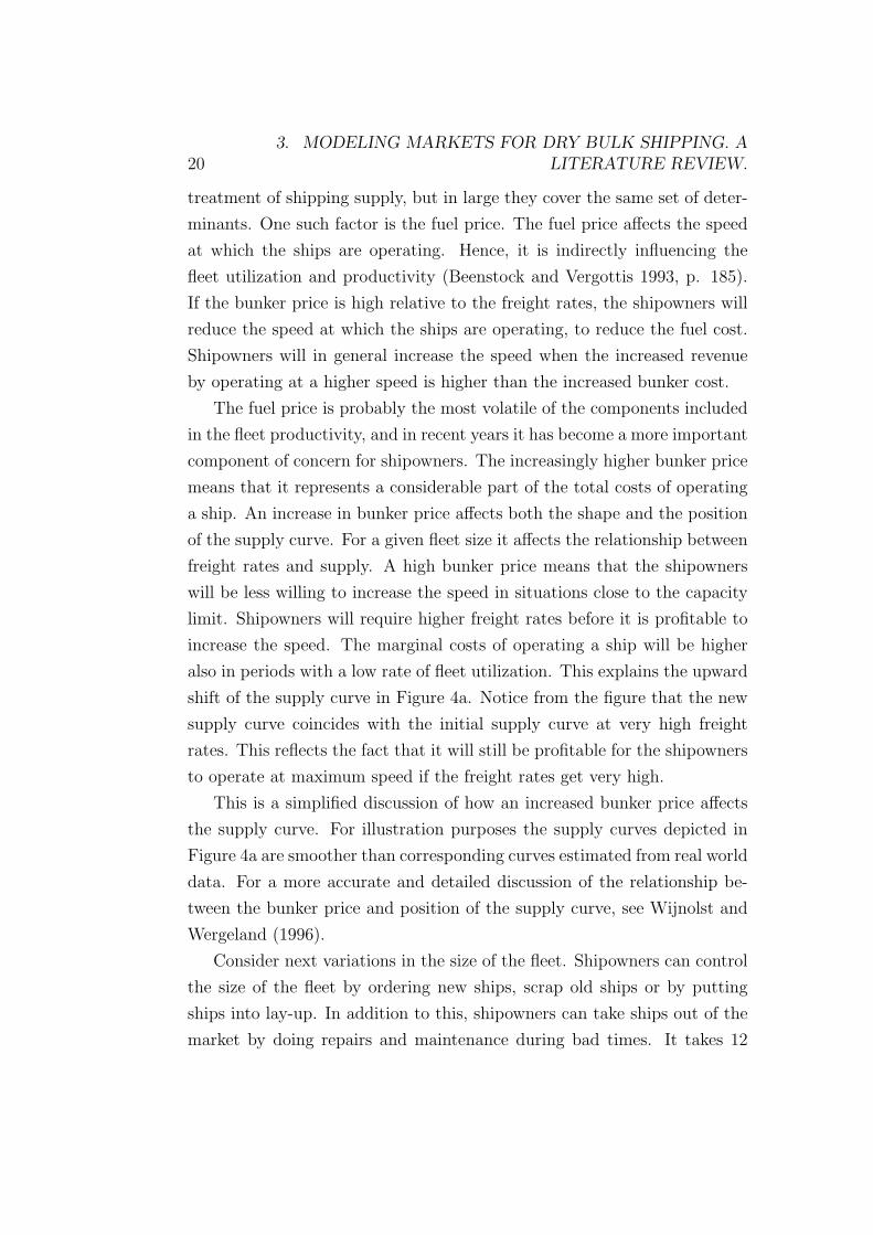
also in periods with a low rate of fleet utilization. This explains the upward
shift of the supply curve in Figure 4a. Notice from the figure that the new
supply curve coincides with the initial supply curve at very high freight
rates. This reflects the fact that it will still be profitable for the shipowners
to operate at maximum speed if the freight rates get very high.
This is a simplified discussion of how an increased bunker price affects
the supply curve. For illustration purposes the supply curves depicted in
Figure 4a are smoother than corresponding curves estimated from real world
data. For a more accurate and detailed discussion of the relationship be-
tween the bunker price and position of the supply curve, see Wijnolst and
Wergeland (1996).
Consider next variations in the size of the fleet. Shipowners can control
the size of the fleet by ordering new ships, scrap old ships or by putting
ships into lay-up. In addition to this, shipowners can take ships out of the
market by doing repairs and maintenance during bad times. It takes 12
3.2. THE SUPPLY OF SHIPPING SERVICES 21F
reig
ht
rate
Tonne miles
a) An increased bunker price
Fre
ight
rate
Tonne miles
b) An increased fleet size
Figure 4: The dashed lines represent the supply curve after the increasedbunker price and fleet size.
months to 3 years to have a new ship delivered (Stopford, 2009, p. 639).
In the long run the size of the fleet is very flexible. When the freight rates
are high, shipowners will order more ships, and the fleet size will increase.
When the freight rates are low, not only will shipowners stop the ordering
of ships, they may also put ships into lay-up and scrap old, inefficient ships
that are costly to run. Part b) of Figure 4 illustrates the effect on the supply
curve of an increased number of deliveries to the shipowners. This figure
is based on the simplifying assumption that the new vessels have the same
voyage cost level as the older vessels.
The time lag from the ordering to the delivery can be challenging. Ship-
ping is a dynamic industry and the market conditions can change rapidly.
During the time it takes to have a ship delivered, the market can be com-
pletely different from how it was when the ship was ordered. In a discrete-
time stochastic equilibrium model of the VLCC market, Adland and Stran-
denes (2004) account for the possibility that the delivery rate is an increas-
ing function of the current freight rate level. They argue that postpone-
ments and cancellations of newbuilding projects may occur in periods with
low freight rates, while newbuilding projects to some degree may be accel-
erated through for instance extensive use of overtime in periods with high
freight rates.
In a short-term time perspective, the size of the fleet is relatively fixed.
Variations in lay-ups correspond to movements along the elastic segment
223. MODELING MARKETS FOR DRY BULK SHIPPING. A
LITERATURE REVIEW.
of the supply curve. The ships will operate as long as the freight rates are
higher than the operating cost (Stopford, 2009, p. 161-162). Adland and
Strandenes (2004) refer to the classical literature, where the lay-up point
is the time charter equivalent spot freight rate at which the shipowner is
indifferent between lay-up and operation. The literature also accounts for
switching costs related to putting the vessel in lay-up. Due to such costs the
ships will operate if the threshold freight rate exceeds the daily operating
cost less the daily lay-up cost (Mossin, 1968). When the freight rates are
lower than this threshold, the ships will be put into lay-up. All ships do not
have the same operating cost, however. Hence, the supply will be gradually
lower as the freight rates are reduced.
Scrapping vessels is another relatively fast response to low freight rates.
As pointed out by for instance Adland and Strandenes (2004) it is optimal
to scrap a vessel if the scrap value exceeds the expected value of continued
trading. They also point out, however, that scrapping decisions may partly
be strategic, since freight rates are negatively related to the remaining fleet,
and the profit of a shipowner tend to increase when other shipowners scrap
their vessels. Adland and Strandenes (2004) specify a model for the VLCC
supply function where the scrapping volume follows a stochastic Poisson
process, letting the expected scrapping volume depend on the freight rates.
I will not enter into a more detailed discussion of such a process, however.
Graphically, the impact of scrapping the most inefficient vessels is a inward
shift of the supply curve, corresponding to a shift from the dashed to the
solid line in Figure 4.
3.3 The demand for shipping services
According to Stopford (2009, p. 139-149) there are five key factors that
influence the demand for sea transport. These five factors are the world
economy, seaborne commodity trades, average haul, random shocks and
transport costs.
Stopford (2009, p. 140) further claims that the world economy has the
strongest impact on the demand for sea transport. There are two aspects
3.3. THE DEMAND FOR SHIPPING SERVICES 23
of the world economy that influence the demand for sea transport; business
cycles and the trade development cycle (Stopford, 2009, p. 140). The
business cycle is ”the most important cause of short-term fluctuations in
seaborne trade and ship demand” (Stopford, 2009, p. 142). The ambition
of this thesis is to study short- and long-term relationships between business
cycle measures and freight rates in dry bulk shipping. The empirical results
are presented in Section 6, and a theoretical discussion is provided in Section
7. The trade development cycle involves the ability of a market to meet the
demand for resources such as food and natural resources (Stopford, 2009,
p. 143).
The second key factor that influences the demand for sea transport is the
structure of the seaborne commodity trades (Stopford 2009, p. 143-146). If,
for example, the processing of a commodity moves away from the resource,
there will be an increased demand for sea transport. It is further obvious
that both the average haul of the trade and random shocks influence the
demand for sea transport (Stopford 2009, p. 146-149). Random shocks
involve for example economic shocks, but can also involve political events
such as wars. The last key factor Stopford includes is transport costs (Stop-
ford, 2009, p. 149). It may seem logical that the transport cost influences
the demand for sea transport. As I will get back to below, however, there
are some controversy on this issue. Stopford (2009, p. 149) argues that
the cost of sea transport is an important factor influencing the long-term
demand for sea transportation.
The NORBULK model by Strandenes and Wergeland (1980) is based on
the assumption that the demand for transportation of dry bulk commodi-
ties is determined by the freight rates, the trade patterns, and variables
reflecting the macroeconomic situation (see Figure 2).
There seems to be a consensus in the literature on how changes in
macroeconomic conditions cause shifts in the demand curve. The literature
is more concerned about the elasticity of shipping demand with respect to
the freight rates. In early contributions, like Tinbergen (1934) and Koop-
mans (1939), the demand was assumed to be independent of the freight
rates. This assumption that demand is completely inelastic with respect
243. MODELING MARKETS FOR DRY BULK SHIPPING. A
LITERATURE REVIEW.
to freight rates was also adopted for instance by Beenstock and Vergottis
(1993, p. 162), who claim that “we have been unable to discover a negative
relationship between demand and freight rates”.
Beenstock and Vergottis (1993, p. 162) also acknowledge the fact that
theory is in favor of an inverse relationship between freight rates and the
demand for shipping services, however, since “higher freight rates will create
an incentive to use other forms of transportations and to import more from
areas closer to the market” (Beenstock and Vergottis, 1993, p. 162). The
reason why freight rates are still often treated exogenously is that there
is a very limited scope for substituting between forms of transportation
and origins of import, at least within a short-term time perspective. In a
longer-term time perspective demand will be more price elastic, since trade
patterns will change as a response to high freight rates..
Another frequently used argument in favor of an inelastic demand is
that the freight rate in general represents a low cost relative to the value of
the commodities transported. This argument in particular means that the
demand for transport of expensive commodities is less sensitive to variations
in freight rates than the demand for transport of lower-priced commodities.
NORBULK is an example of a model based on the assumption that de-
mand is inversely related to the freight rate. The relationship was estimated
to be very inelastic, however. Still, Strandenes and Wergeland (1980) argue
that it is potentially important to account for the price elasticity in both
supply and demand. More recently, the maritime economic literature has
suggested a highly non-linear demand curve, see for instance Adland and
Strandenes (2004) for a brief review of this literature. The basic idea is
that demand is in general very inelastic, but “that the demand for ocean
transportation becomes more elastic with respect to freight rates at high
freight rates until the demand becomes perfectly elastic at some unknown
but extremely high freight rate level” (Adland and Strandenes 2004). This
is illustrated in Figure 5, which also includes a supply curve of the classical
shape.
Adland and Strandenes (2004) offer the following set of explanations for
the elastic part of the demand curve:
3.3. THE DEMAND FOR SHIPPING SERVICES 25
Fre
ight
rate
Tonne miles
Demand
Supply
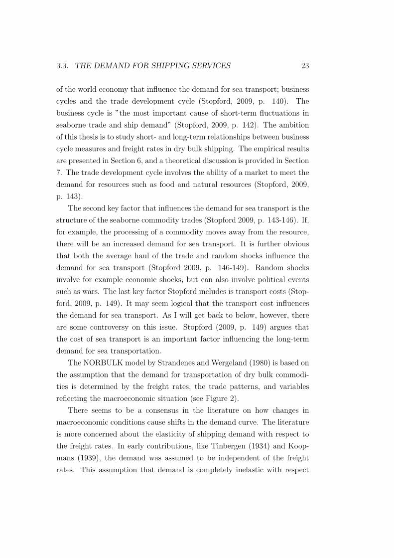
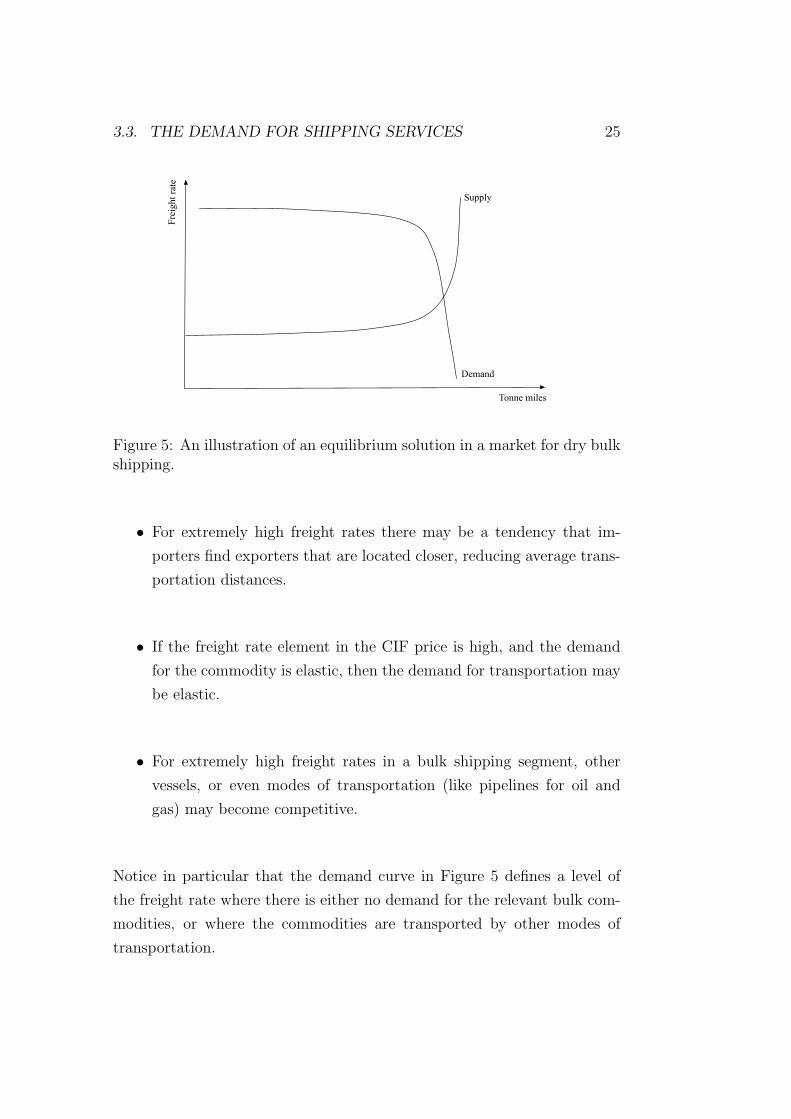
Figure 5: An illustration of an equilibrium solution in a market for dry bulkshipping.
• For extremely high freight rates there may be a tendency that im-
porters find exporters that are located closer, reducing average trans-
portation distances.
• If the freight rate element in the CIF price is high, and the demand
for the commodity is elastic, then the demand for transportation may
be elastic.
• For extremely high freight rates in a bulk shipping segment, other
vessels, or even modes of transportation (like pipelines for oil and
gas) may become competitive.
Notice in particular that the demand curve in Figure 5 defines a level of
the freight rate where there is either no demand for the relevant bulk com-
modities, or where the commodities are transported by other modes of
transportation.
264. OBSERVED VARIATIONS IN SHIPPING VOLUMES AND
FREIGHT RATES
3.4 Shipping market equilibrium
According to Stopford (2009, p. 175 - 231) shipowners operate in four
separate, but interlinked markets: freight, newbuilding, scrapping and sale
& purchase. This thesis focuses primarily on the freight market. It was
clear from Section 3.2, however, that decisions made on the other three
markets affect the position of the supply curve, and that a new equilibrium
freight rate will emerge as a response to shocks in those markets.
A shipping market equilibrium is represented by the freight rate where
the demand equals the supply of shipping services, that is at the point
where the two curves intersect in Figure 5. Due to the nonlinearities of
the curves it is obvious that the impact of demand and/or supply shocks
is highly dependent on the initial situation. Consider a positive demand
shock, for instance due to a general economic growth, leading to increased
trade and increased demand for ocean transportation. This corresponds to
an outward shift of the demand curve. If this happens in a situation with a
low degree of fleet utilization, the main effect of the shift is that the number
of ships in lay-up will be reduced. Hence, the tonne miles of transported
commodities will increase substantially, while the impact on freight rates
will be relatively marginal. The situation is the opposite if there is a very
high degree of fleet utilization initially. In a short-term time perspective a
positive demand shock then leads to a substantial increase in freight rates,
while the transported tonnage increases marginally.
I will do more use of this modeling framework in Section 7, attempting
to explain some of the empirical results from Section 6.
4 Observed variations in shipping volumes
and freight rates
As a starting point for an analysis of the market for transportation of dry
bulk cargo it is useful to study how the key variables in this market have
developed over time. My information on the BFI refer to daily observations
27
back to 1985, while data on total bulker sales are available only after 1995.
The regressions performed in the empirical section refers to the entire period
1985-2009. For a direct comparison, however, the observations presented
below are restricted to the period 1995-2009.
0
0
02000
2000
20004000
4000
40006000
6000
60008000
8000
800010000
1000
0
10000BFI monthly
BFI m
onth
ly
BFI monthly1995m1
1995m1
1995m12000m1
2000m1
2000m12005m1
2005m1
2005m12010m1
2010m1
2010m1time
time
time
a) The level of the BFI
-4000
-400
0
-4000-2000
-200
0
-20000
0
02000
2000
2000First difference of BFI
Firs
t di
ffer
ence
of B
FI
First difference of BFI1995m1
1995m1
1995m12000m1
2000m1
2000m12005m1
2005m1
2005m12010m1
2010m1
2010m1time
time
time
b) The first differences of the BFI
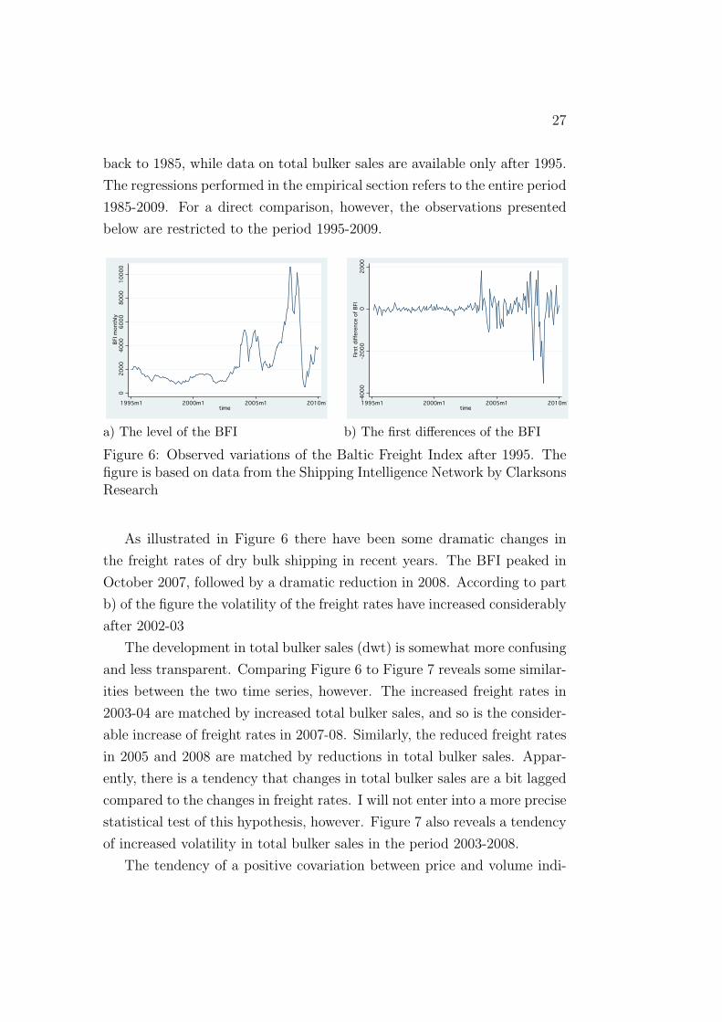
Figure 6: Observed variations of the Baltic Freight Index after 1995. Thefigure is based on data from the Shipping Intelligence Network by ClarksonsResearch
As illustrated in Figure 6 there have been some dramatic changes in
the freight rates of dry bulk shipping in recent years. The BFI peaked in
October 2007, followed by a dramatic reduction in 2008. According to part
b) of the figure the volatility of the freight rates have increased considerably
after 2002-03
The development in total bulker sales (dwt) is somewhat more confusing
and less transparent. Comparing Figure 6 to Figure 7 reveals some similar-
ities between the two time series, however. The increased freight rates in
2003-04 are matched by increased total bulker sales, and so is the consider-
able increase of freight rates in 2007-08. Similarly, the reduced freight rates
in 2005 and 2008 are matched by reductions in total bulker sales. Appar-
ently, there is a tendency that changes in total bulker sales are a bit lagged
compared to the changes in freight rates. I will not enter into a more precise
statistical test of this hypothesis, however. Figure 7 also reveals a tendency
of increased volatility in total bulker sales in the period 2003-2008.
The tendency of a positive covariation between price and volume indi-

284. OBSERVED VARIATIONS IN SHIPPING VOLUMES AND
FREIGHT RATES
cates that the development is basically driven by demand shifts. At the
same time the increased volatility in recent years indicates that the fleet is
operating close to its current capacity limit. In periods with a high capac-
ity utilization positive adjustments in supply will be sluggish, and demand
shocks have a large impact on freight rates. This is a reasonable explana-
tion of the drastically increased freight rates in the recent periods of boom
in the world economy.
0
0
02000000
2000
000
20000004000000
4000
000
40000006000000
6000
000
60000008000000
8000
0008000000Total Bulker Sales DWT
Tota
l Bul
ker S
ales
DW
T
Total Bulker Sales DWT1995m1
1995m1
1995m12000m1
2000m1
2000m12005m1
2005m1
2005m12010m1
2010m1
2010m1time
time
time
a) The level of total bulker sales
-4000000
-400
0000
-4000000-2000000
-200
0000
-20000000
0
02000000
2000
000
20000004000000
4000
0004000000First difference of Total Bulker Sales DWT
Firs
t di
ffer
ence
of T
otal
Bul
ker S
ales
DW
T
First difference of Total Bulker Sales DWT1995m1
1995m1
1995m12000m1
2000m1
2000m12005m1
2005m1
2005m12010m1
2010m1
2010m1time
time
time
b) The first differences of total bulkersales
Figure 7: Observed variations of the total bulker sales in dwt.
The recession following the financial crisis also reduced the demand for
ocean transportation of dry bulk commodities, and the BFI was reduced
from 10527.45 to 577.28 in 14 months. This reduction in freight rates is
not only a result of a reduced demand, however. The recession coincided
with an increased fleet size, responding to the high freight rates in the
preceding years. The dramatic reduction in freight rates results from the
combination of this lagged supply effect and the unanticipated reduction in
demand. Eventually, the freight rates reached a level where the ship-owners
responded by lay-ups. I will elaborate more on those issues in Section 7.4.
The volatility in freight rates and freight volumes seems to be somewhat
reduced towards the end of the period covered by Figures 6 and 7. This
probably corresponds to a situation where the market is no longer operating
in the most inelastic segment of the supply curve.
29
5 Some basic issues in time series analyses
As pointed out in the introduction the ambition of this thesis is to study
relationships between freight rates in dry bulk shipping and alternative
indicators of business cycles. The basic hypothesis is that the business cycle
influences the freight rates trough the impact on the demand for shipping
services. This section focuses on the econometric techniques I will be using
to study this hypothesis.
5.1 Stationarity and spurious regression
In time series analysis an important distinction is between stationary and
non-stationary variables. For an explanation of this distinction consider
first the more general specification of autoregressive time series variables.
An autoregressive time series variable, yt, depends on past values of itself
and an independent error term with expectation 0 and constant variance,
σ2. Consider first the following specification of a time series variable:
yt = α +n∑
i=1
ρiyt−i + vt, (1)
Here, vt is the error term, and yt−i is the value of the variable at time
period t − i. In cases where yt has a unit root, α is a drift component
resulting in a trended behaviour. The variable yt is autoregressive of order
n, AR(n), if n represents the number of lags that are statistically significant
different from 0. In the discussion of stationary and non-stationary variables
I will be referring to variables that are autoregressive of order 1, AR(1),
defined by Equation (2).
yt = α + ρyt−1 + vt (2)
A stationary time series represents a mean reverting stochastic process,
corresponding to a situation where |ρ| < 1 in Equation (2). For a stationary
variable both the expected value and the variance will be constant; E(yt) =
α and Var(yt) = Var(vt) = σ2. In addition, the covariance between two
30 5. SOME BASIC ISSUES IN TIME SERIES ANALYSES
values in the series must depend only on the time difference, not the actual
time they were observed; Cov(yt, yt + h) depends on h and not on t (see
Wooldridge, 2008, Chapter 11.1).
Assume next that ρ = ±1. The variance then increases over time,
Var(yt) = tσ2, and so is the expected value for the case with a positive
drift component (α > 0); E(yt) = tα + y0 (see Hill et al., 2008, p. 332).
Hence, the conditions for stationarity are violated. In the case where ρ = 1
the resulting model is represented by yt = α + yt−1 + vt. The variable yt
is then non-stationary, and the model is a random walk with drift. For
non-stationary variables a shock has a permanent impact on the stochastic
process, which is not mean reverting. The best prediction of a future value
will always be the present value (see Wooldridge, 2008, Chapter 11.3).
A random walk is a unit root process. The drift component defines
an upward trend in the case with α > 0. In such a case the model cor-
responds to a time series fluctuating without a clear pattern around an
upward trend. As pointed out for instance by Hill et al. (2008, p. 333)
the trend behaviour may be strengthened, by introducing a time trend, δt,
resulting in a quadratic trend in the random walk model:
yt = α + δt+ yt−1 + vt (3)
I do not consider the possibility that |ρ| > 1, which corresponds to explosive
time series.
A non-stationary variable that becomes stationary if we differentiate it d
times is said to be integrated of order d, I(d). Hence, a variable that is I(2)
must be differentiated twice to become stationary; ∆yt = yt − yt−1 − yt−2.
A stationary variable is integrated of order 0, I(0).
Consider a regression of y on x,
yt = α + βxt + et. (4)
et is the error term. Such a regression of two non-stationary variables does
not give reliable results. A regression of I(1) variables generally results in
low standard errors, inflated t-values and artificially high R2-values. Hence,

5.1. STATIONARITY AND SPURIOUS REGRESSION 31
there is an imminent risk of making type 2-errors is, and the results may in-
dicate a statistically significant relationship even though such a relationship
does not exists. This reflects a spurious regression problem.
One obvious solution to this problem is to differentiate each variable the
number of times that makes it stationary. Such a model specification only
provides an estimate of the short-term effect of a change in the explanatory
variable, however. For most problems it is essential to explain and predict
more long-term consequences of an exogenous shock. As will be clear from
the discussion in the subsequent section, there is one exception where re-
liable estimates result from OLS regressions on non-stationary variables in
level form.
A first step towards such a procedure is to test for unit roots. Several
tests have been developed for this purpose. The technique I will be using
is the Dickey-Fuller test (Dickey and Fuller, 1979). A variable has a unit
root, is non-stationary, if ρ = 1 in Equation (2). Hence, the null hypothesis
of the Dickey-Fuller test is that the variable has a unit root. The test is
based on a model formulation where yt−1 is subtracted from both sides of
Equation (2):
yt − yt−1 = α + ρyt−1 − yt−1 + vt = α + (ρ− 1)yt−1 + vt (5)
Hence, testing for nonstationarity is equivalent to testing the hypothesis
that ω = ρ− 1 = 0 in Equation (6):
∆yt = α + ωyt−1 + vt (6)
We can now test H0: ω = 0 against H1: ω < 0. In a case where H0 is not
rejected, we conclude that ρ = 1 and that yt is non-stationary.
In performing the Dickey-Fuller test for unit roots it is important to
know that the t statistic does not have an approximate standard normal
distribution, since yt−1 is I(1) (see for instance Wooldridge 2008, Chapter
18.2). This means that the standard t-distribution does not provide reliable
critical values for the Dickey-Fuller test. Instead, critical values are tab-
ulated for the Dickey-Fuller-distribution, originally introduced by Dickey
and Fuller, and later refined by others (Wooldridge, 2008, Chapter 18.2).

32 5. SOME BASIC ISSUES IN TIME SERIES ANALYSES
Many variables are autoregressive of orders higher than one. When
this is the case, we must use the augmented Dickey-Fuller test. The aug-
mented Dickey-Fuller test includes several lags in order to control for serial
correlation. Enough lags should be included to control for all the serial
correlation in the variable. Including too many lags is not recommendable,
however, since adding more lags means that we loose degrees of freedom in
the regression. The appropriate number of lags involved can for instance
be determined from the last significant lag criterion (Ng and Perron, 1995).
This corresponds to a method where the number of lags accounted for is
reduced successively from a very high number down to the last lag found
to be significantly different from zero. A model specification with a drift
component α and k lags is given by:
∆yt = α + ωyt−1 + λ1∆yt−1 + · · ·+ λt−k∆yt−k + vt (7)
The null hypothesis for the unit root test is of course still that ω = 0 against
the alternative hypothesis of ω < 0. Changes in yt respond to the lagged
changes of the variable. If the variable is non-stationary, however, ∆yt is
totally insensitive to the value of the variable in the previous period, yt−1.
5.2 Cointegration
There is one situation in which the result from a regression of two non-
stationary time series is not spurious. This situation of relates both to the
integration order of the two variables and to the integration order of the
corresponding error term. Assume that the two variables are both I(1), and
consider the following regression of yt on xt:
yt = α + βxt + et (8)
The error term is then just a linear combination of yt and xt:
et = yt − α− βxt (9)
In most cases the error term will be non-stationary in such a case, but
there may be some exceptions where the linear combination is stationary,
5.2. COINTEGRATION 33
see for instance Koop (2008, p. 218) or Wooldridge (2008, Chapter 18.4). If
the linear combination is I(0), yt and xt are cointegrated. This will be the
case if the two variables follow the same stochastic trend, and are related
through an equilibrium relationship. In such a case we can run a standard
regression of one variable on the other without having to worry about the
spurious regression problem.
There are many examples in the literature on economics and finance
where equilibrium relationships give scenarios of cointegrated variables.
Wooldridge (2008, Chapter 18.4) refers to results on the relationship be-
tween short- and long-term interest rates, while Koop (2008, p.219) studies
time series for the prices of close substitutes. Based on arbitrage arguments
they explain why differences between such variables tend to be relatively
stable over time, and return to an equilibrium level after a shock.
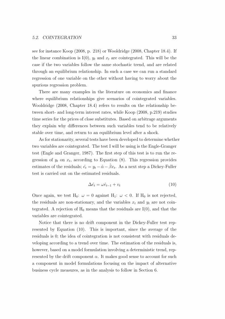
As for stationarity, several tests have been developed to determine whether
two variables are cointegrated. The test I will be using is the Engle-Granger
test (Engle and Granger, 1987). The first step of this test is to run the re-
gression of yt on xt, according to Equation (8). This regression provides
estimates of the residuals; et = yt− α− βxt. As a next step a Dickey-Fuller
test is carried out on the estimated residuals.
∆et = ωet−1 + vt (10)
Once again, we test H0: ω = 0 against H1: ω < 0. If H0 is not rejected,
the residuals are non-stationary, and the variables xt and yt are not coin-
tegrated. A rejection of H0 means that the residuals are I(0), and that the
variables are cointegrated.
Notice that there is no drift component in the Dickey-Fuller test rep-
resented by Equation (10). This is important, since the average of the
residuals is 0; the idea of cointegration is not consistent with residuals de-
veloping according to a trend over time. The estimation of the residuals is,
however, based on a model formulation involving a deterministic trend, rep-
resented by the drift component α. It makes good sense to account for such
a component in model formulations focusing on the impact of alternative
business cycle measures, as in the analysis to follow in Section 6.
34 5. SOME BASIC ISSUES IN TIME SERIES ANALYSES
The Engle-Granger test is simple to perform, but it has some limita-
tions. One limitation is that the two variables that are being tested for
cointegration have to be integrated of the same order. As will be clear in
Section 6, however, this is not a problem in my dataset, and this potential
limitation of the testing procedure is not a problem in my analysis.
A very common mistake when performing the Engle-Granger test is to
use the critical values tabulated for the Dickey-Fuller-distribution when the
residuals are tested for stationarity. This is not correct, since we are testing
estimated rather than actual residuals. A more appropriate approach is
therefore to use critical values originally tabulated by Engle and Granger
(1987) and MacKinnon (1991). MacKinnon has recently (MacKinnon 2010)
made available a working paper providing more accurate critical values,
covering more cases than the original paper. The new critical values are
based on simulations with far more replications than in the original paper.
The critical values used in Section 6 are calculated from the tables and
functional forms presented in MacKinnon (2010).
5.3 The error correction model
A conclusion that two variables are cointegrated offers very interesting and
important information. Cointegration means that there is an equilibrium
relationship between the two variables. There can be several reasons for
such an equilibrium relationship. One of the variables can for example
depend on the other, or they may both depend on the same exogenous
factors. Either way, establishing an equlibrium relationship is an important
finding.
It is also important that cointegration justifies the use of an error cor-
rection model. This result is based on the Granger representation theorem
(Engle and Granger, 1987). An error correction model is more specific on
the dynamics involved in a relationship between two variables, it captures
both short-term dynamics and long run effects. The estimate of the cointe-
gration parameter β in Equation (8) provides information on the long-term
influence of a shock in the exogenous variable. The short-term dynamics

5.3. THE ERROR CORRECTION MODEL 35
are represented by the contemporaneous change in xt, and by the intro-
duction of the error term of the previous period (Wooldridge 2008, Chap-
ter 18.4). It follows from Equation (9) that this error term is defined by
et = yt − α − βxt, while the estimated error term from the cointegration
regression is et = yt − α − βxt. An error correction model is then defined
by the following equation:
∆yt = µ+ γ∆xt + δet−1 + ut = µ+ γ∆xt + δ(yt−1 − α− βxt−1) + ut (11)
ut is the error term in the error correction model, corresponding to the
standard assumption of an OLS regression. In some applications of the
error correction model β is assumed to be known, and the error correction
term defined to be yt − βxt. The version represented by Equation (11),
based on the cointegration regression, is often called the Engle-Granger
two-step procedure, see Wooldridge (2008, Chapter 18.4) or Koop (2007, p.
224). It is also possible to find applications of the error correction model
where the changes in the exogenous variable is lagged one period, which
means that ∆xt−1 rather than ∆xt appears in the model formulation (see
for instance Verbeek (2008, p. 332)). For the problems I will be studying,
however, I find the model formulation with a contemporaneous change in
xt to be a reasonable representation of the short-term relationship between
the variables. This is also according to the procedure recommended by for
example Koop (2008, p. 225). The lagging of the error correction term,
et−1, contributes with an adjustment to the deviation from equilibrium in
the previous period.
As mentioned above β in Equation (11) is the long run multiplier re-
lated to a change in xt from its equilibrium value, while γ represents the
short-term effect. The parameter δ reflects the equilibrium adjustment
mechanism. If yt−1 > α + βxt−1 the dependent variable is higher than
the equilibrium value. The error correction term contributes to close this
gap, corresponding to a situation with δ < 0. Similarly, a value of δ < 0
contributes to increase the prediction of the dependent variable towards
equilibrium in cases where yt−1 < α+ βxt−1. The parameter estimate δ of-
fers an estimate of how long time it takes before a deviation from the long
366. SHORT- AND LONG-TERM RELATIONSHIPS BETWEEN
FREIGHT RATES AND BUSINESS CYCLE MEASURES
run equilibrium is corrected for. A value of δ = −0.5 for example means
that half of the error is corrected for in the next period.
The error correction model in Equation (11) has all the properties re-
lated to standard OLS regressions, with statistics like t-values, P -values
and R2 available for the evaluation of results. Equation (11) is, however,
a simple version of the model; neither the dependent nor the independent
variables are lagged.
6 Short- and long-term relationships
between freight rates and business cycle
measures
In this section the econometric techniques explained above are used to study
possible short and long-term relationships between freight rates in dry bulk
shipping and some measures of the business cycle and trade flows. Varia-
tions in economic activities may differ considerably between continents and
countries; business cycles are not always closely geographically coordinated.
An increased economic activity in one geographic area may have a larger
impact on trade flows and the demand for shipping services than a corre-
sponding increased activity somewhere else. Hence, measures of production
are introduced for different geographies. In addition the analysis focuses on
how information on specific trade flows contributes to explain variations in
shipping freight rates.
As stated in the introduction my ambition is to study short and long-
term effects of demand shocks in the market for shipping services. First,
testing for cointegration gives important information on possible long-term
equilibria between the relevant time series. If variables are cointegrated, an
error correction model contributes with more specific information on the
short- and long-term dynamics involved. The presentation of results will
be organized as follows:
• testing the time series for stationarity
6.1. TESTING BASED ON QUARTERLY DATA 37
• finding the integration order
• testing for cointegration
• running error correction models
This procedure will be performed for both quarterly and monthly data, in
Section 6.1 and Section 6.2, respectively.
Some of the time series used in the analysis to follow were adjusted for
seasonal variations. To make the results from the regressions as comparable
as possible, the rest of the times series were also adjusted for seasonal
variations. This adjustment was done according to the technique X-12-
ARIMA8, which is a software used for all official seasonal adjustments by
the US Census Bureau. Alternatively, seasonal variations can be accounted
for by introducing seasonal dummies. Since seasonal variations were already
removed from some of the available time series, however, I chose to adjust
the time series according to the described technique for all the regressions
to follow.
Notice also that all the variables are represented by their logarithmic
values in the regressions to be presented. Interpretations in terms of elastic-
ities facilitate the analysis in a framework where the variables are measured
in very different units, and the choice of logarithmic specifications are ac-
cording to standard procedures in the literature.
6.1 Testing based on quarterly data
One basic hypothesis to be studied is that both the demand for shipping
services and shipping rates are positively related to the business cycle. The
most obvious choice of a business cycle measure is the gross domestic prod-
uct (gdp) for relevant geographies. Data on gdp are not available for shorter
time periods than quarters. As mentioned in Section 2.1 the daily time se-
ries on shipping rates are converted into quarterly series, by simple averag-
ing. Due to the considerable noise involved in data defined for a very short
8See http://www.census.gov/srd/www/x12a/
386. SHORT- AND LONG-TERM RELATIONSHIPS BETWEEN
FREIGHT RATES AND BUSINESS CYCLE MEASURES
period, a conversion into monthly or quarterly averages may be a preferred
approach even if daily data were available.
6.1.1 Stationarity of freight rates and some business
cycle measures
In this section the augmented Dickey-Fuller test for stationarity is used
on quarterly times series for shipping rates and gross domestic product
for different geographical areas. The gdp of OECD is used as a proxy
variable for world production, while the gdp of the US, Japan, and China
represents the economic activity and demand for shipping services in three
very important countries in world trade. The number of lags involved is
determined from the last significant lag criterion, see Section 5.1.
As mentioned in Section 5.1 a unit root process may incorporate both a
drift and a trend component, see Equation (3). In testing for stationarity
it is in general not clear, however, that drift (α) and trend (δt) components
should be included. The choice of a model specification depends on a pri-
ori knowledge of the specific variable. Concerning freight rates in dry bulk
shipping, there is no a priori reason to expect a specific trend development,
see for instance Figure 14a and Figure 14b in Appendix B. Observed time
series of gdp, on the contrary, tend to reflect a rising trend. Only if the
observations indicate a convex trend the model formulation should include
both the drift and the trend component in Equation (3). Such observations
are the rationale for the model specifications underlying the results in Table
1, ignoring trend components. I have, however, experimented with model
formulations with and without time and trend components. The conclu-
sions on stationarity proved not to be sensitive to how such components
are accounted for in the model specifications. The model specification un-
derlying the result for the Baltic Freight Index (BFI) in Table 1 ignores
both a drift and a trend component. The results for the gdp-measures are
based on model specifications with a drift component, but without a trend
component.
According to the results referred in Table 1 all the quarterly variables are
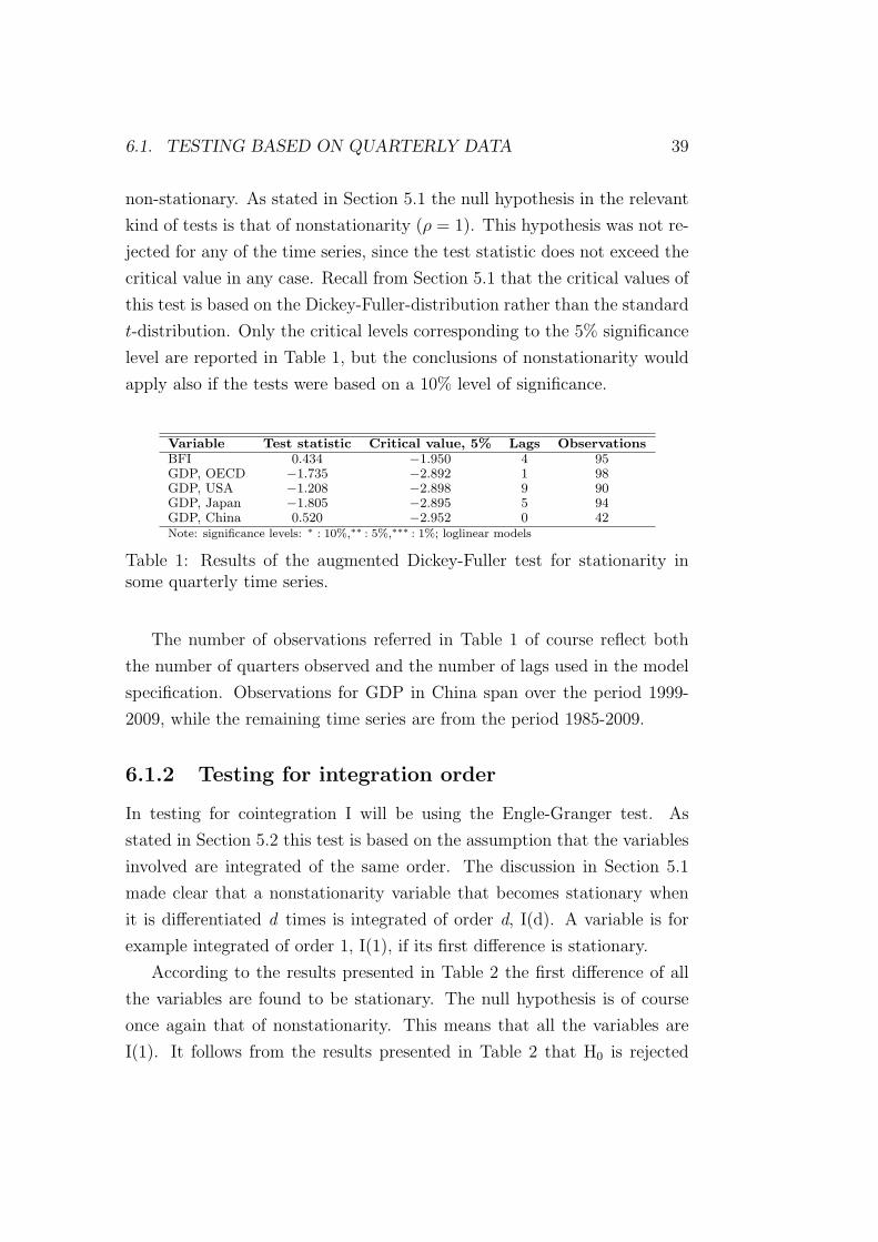
6.1. TESTING BASED ON QUARTERLY DATA 39
non-stationary. As stated in Section 5.1 the null hypothesis in the relevant
kind of tests is that of nonstationarity (ρ = 1). This hypothesis was not re-
jected for any of the time series, since the test statistic does not exceed the
critical value in any case. Recall from Section 5.1 that the critical values of
this test is based on the Dickey-Fuller-distribution rather than the standard
t-distribution. Only the critical levels corresponding to the 5% significance
level are reported in Table 1, but the conclusions of nonstationarity would
apply also if the tests were based on a 10% level of significance.
Variable Test statistic Critical value, 5% Lags ObservationsBFI 0.434 −1.950 4 95GDP, OECD −1.735 −2.892 1 98GDP, USA −1.208 −2.898 9 90GDP, Japan −1.805 −2.895 5 94GDP, China 0.520 −2.952 0 42Note: significance levels: ∗ : 10%,∗∗ : 5%,∗∗∗ : 1%; loglinear models
Table 1: Results of the augmented Dickey-Fuller test for stationarity insome quarterly time series.
The number of observations referred in Table 1 of course reflect both
the number of quarters observed and the number of lags used in the model
specification. Observations for GDP in China span over the period 1999-
2009, while the remaining time series are from the period 1985-2009.
6.1.2 Testing for integration order
In testing for cointegration I will be using the Engle-Granger test. As
stated in Section 5.2 this test is based on the assumption that the variables
involved are integrated of the same order. The discussion in Section 5.1
made clear that a nonstationarity variable that becomes stationary when
it is differentiated d times is integrated of order d, I(d). A variable is for
example integrated of order 1, I(1), if its first difference is stationary.
According to the results presented in Table 2 the first difference of all
the variables are found to be stationary. The null hypothesis is of course
once again that of nonstationarity. This means that all the variables are
I(1). It follows from the results presented in Table 2 that H0 is rejected
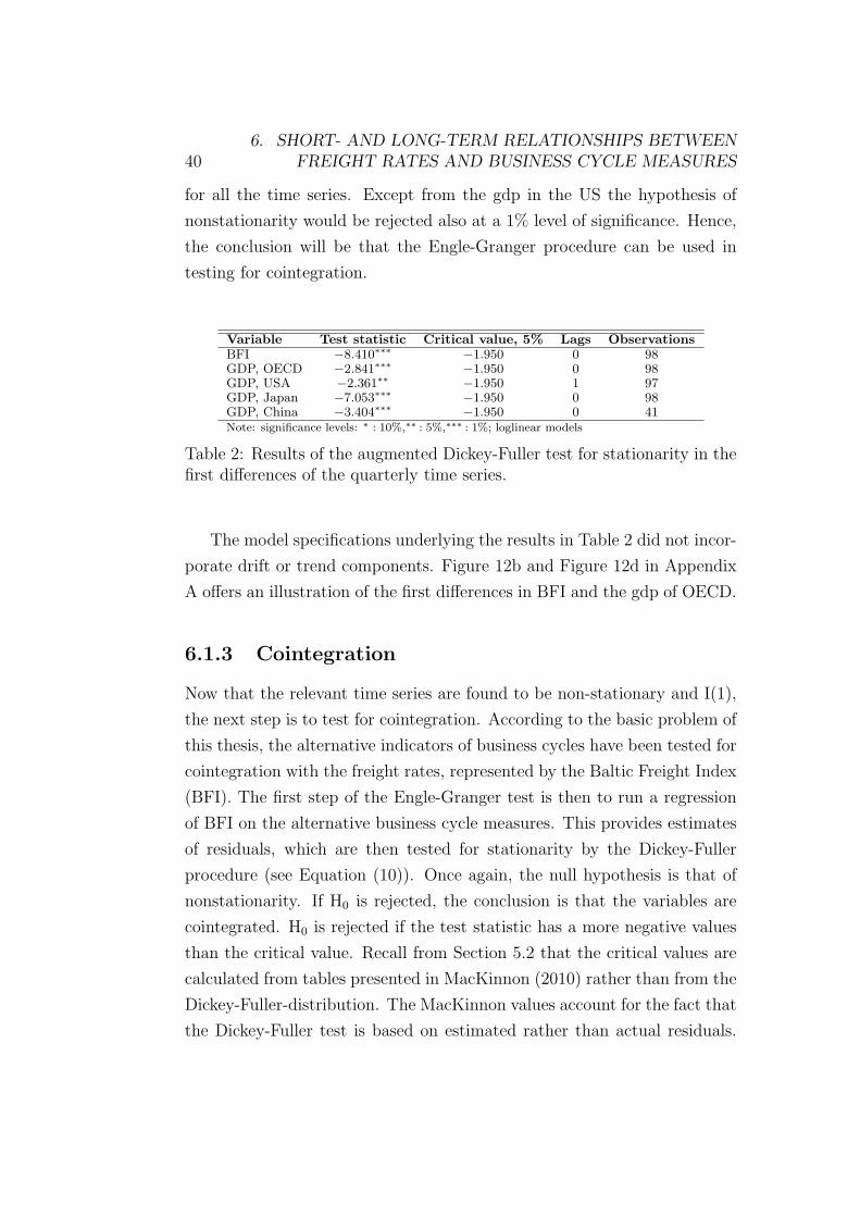
406. SHORT- AND LONG-TERM RELATIONSHIPS BETWEEN
FREIGHT RATES AND BUSINESS CYCLE MEASURES
for all the time series. Except from the gdp in the US the hypothesis of
nonstationarity would be rejected also at a 1% level of significance. Hence,
the conclusion will be that the Engle-Granger procedure can be used in
testing for cointegration.
Variable Test statistic Critical value, 5% Lags ObservationsBFI −8.410∗∗∗ −1.950 0 98GDP, OECD −2.841∗∗∗ −1.950 0 98GDP, USA −2.361∗∗ −1.950 1 97GDP, Japan −7.053∗∗∗ −1.950 0 98GDP, China −3.404∗∗∗ −1.950 0 41Note: significance levels: ∗ : 10%,∗∗ : 5%,∗∗∗ : 1%; loglinear models
Table 2: Results of the augmented Dickey-Fuller test for stationarity in thefirst differences of the quarterly time series.
The model specifications underlying the results in Table 2 did not incor-
porate drift or trend components. Figure 12b and Figure 12d in Appendix
A offers an illustration of the first differences in BFI and the gdp of OECD.
6.1.3 Cointegration
Now that the relevant time series are found to be non-stationary and I(1),
the next step is to test for cointegration. According to the basic problem of
this thesis, the alternative indicators of business cycles have been tested for
cointegration with the freight rates, represented by the Baltic Freight Index
(BFI). The first step of the Engle-Granger test is then to run a regression
of BFI on the alternative business cycle measures. This provides estimates
of residuals, which are then tested for stationarity by the Dickey-Fuller
procedure (see Equation (10)). Once again, the null hypothesis is that of
nonstationarity. If H0 is rejected, the conclusion is that the variables are
cointegrated. H0 is rejected if the test statistic has a more negative values
than the critical value. Recall from Section 5.2 that the critical values are
calculated from tables presented in MacKinnon (2010) rather than from the
Dickey-Fuller-distribution. The MacKinnon values account for the fact that
the Dickey-Fuller test is based on estimated rather than actual residuals.

6.1. TESTING BASED ON QUARTERLY DATA 41
The results of the Engle-Granger test is presented in Table 3.
Variable Test statistic Critical value, 5% Lags ObservationsGDP, OECD −3.485∗∗ −3.3992 1 98GDP, USA −3.444∗∗ −3.3992 1 98GDP, Japan −4.012∗∗ −3.4005 3 96GDP, China −3.893∗∗ −3.4973 3 39Note: significance levels: ∗ : 10%,∗∗ : 5%,∗∗∗ : 1%; loglinear models
Table 3: Results of the Engle-Granger test for for cointegration with theBaltic Freight Index (BFI)
According to the results presented in Table 3, the H0 of no cointegration
is rejected for all the time series, at a significance level of 5%. Hence, the
conclusion is that the alternative business cycle indicators are cointegrated
with the BFI. The conclusion for the gdp of Japan is almost valid for a
significance level of 1%, which corresponds to a critical value of −4.013.
The conclusion that the business cycle measures are cointegrated with
the BFI is interesting and important. It means that there is an equilib-
rium relationship between the business cycle and the freight rates in dry
bulk shipping. This corresponds to an interpretation where the demand
for shipping services reflects the variations in production. Changes in the
business cycle situation then initiate forces pulling the market for ship-
ping services towards a new equilibrium. In other words, the relationship
between the BFI and alternative gdp indicators tend to converge towards
a long-term equilibrium solution. The fact that all the gdp-measures are
cointegrated with the BFI may reflect a tendency of long-term covariation
between the business cycles in different geographies.
A reasonable hypothesis is that short- and medium-term consequences
of changes in production are sensitive to where such changes find place.
This hypothesis will now be discussed within the framework of the error
correction model.
426. SHORT- AND LONG-TERM RELATIONSHIPS BETWEEN
FREIGHT RATES AND BUSINESS CYCLE MEASURES
6.1.4 Results based on Error Correction Models
According to the Granger representation theorem (Engle and Granger,
1987), the presence of cointegration justifies the use of an error correction
model. The results to be presented follow from an Engle-Granger two-step
procedure, based on estimated error terms from the cointegration regression
(et = yt − α− βxt), represented by Equation (11).
Let yt denote the freight rate in dry bulk shipping (BFI) at time period
t, while xt denotes the gdp in a specific geography at the same period
and ut is a log normally distributed error term. Since all the variables are
represented by their natural logarithm, the relevant error correction models
is then given by the following regression model:
∆(ln yt) = µ+ γ∆(lnxt) + δet−1 + ut (12)
This is basically according to the model formulation suggested by both
Wooldridge (2008, p. 643) and Koop (2008, p. 224). An estimate of the
parameter γ represents the immediate percentage change in the BFI as a
response to a 1% change in the relevant gdp measure. The value of the
parameter δ captures the time required before a deviation from equilibrium
is corrected for. In other words, δ represents the percentage of the deviation
that is corrected for within one time period.
Consider first the results for the gdp of the entire OECD area:
∆(ln yt) = − 0.082
(0.036)
+ 15.210
(4.316)
∆(lnxOECDt )− 0.161
(0.053)
eOECDt−1 (13)
Here, the standard errors are given in parentheses under the parameter
estimates. All the parameter estimates are significantly different from zero.
The P -values corresponding to γ and δ are 0.001 and 0.003, respectively.
The results mean that
• a 1% change in the gdp growth in the OECD area immediately causes
a 15.2% change in the growth rate of the BFI
6.1. TESTING BASED ON QUARTERLY DATA 43
• about 16% of the deviation from the equilibrium between the BFI and
the gdp of OECD will be corrected in the subsequent quarter
Those estimate results are based on 99 observations (quarters), and the
model explains about 16.6% of the variation in the logarithm of the changes
in dry bulk freight rates (R2adj ≈ 0.1658).
The results from an error correction model specification for USA, Japan,
and China are given by the following equations:
∆(ln yt) = − 0.048
(0,037)
+ 9.009
(4.218)
∆(lnxUSAt )− 0.145
(0.055)
eUSAt−1 (14)
∆(ln yt) = − 0.006
(0.024)
+ 1.892
(0.456)
∆(lnxJapant )− 0.203
(0.064)
eJapant−1 (15)
∆(ln yt) = − 0.111
(0.078)
+ 4.233
(1.733)
∆(lnxChinat )− 0.314
(0.111)
eChinat−1 (16)
Notice first from the results that the immediate relative effect of a change
in the gdp is larger for the OECD as a whole than for each of the three coun-
tries separately. It is not obvious how this should be interpreted. In such
an interpretation care should be taken to the fact that gdp and business
cycles tend to spread across countries and continents. Hence, the gdp of
different countries tend to covariate. One possible explanation of the results
is, however, that the gdp of OECD is a more satisfactory measure of the
worldwide business cycle than the measures covering smaller geographies.
An increased overall production in the OECD area is typically followed by
increased trade and increased demand for shipping services. The US econ-
omy can also be argued to be a good proxy variable of global growth, trade
and shipping volumes, while the economic development in Japan probably
is more weakly related to the global business cycle. This may also apply
to China, but China represents a very large and strongly growing market
446. SHORT- AND LONG-TERM RELATIONSHIPS BETWEEN
FREIGHT RATES AND BUSINESS CYCLE MEASURES
for trade and shipping services. This is one possible explanation for the
different estimates of the contemporaneous change in gdp’s, γ.
Recall that the estimates for China are based on a relatively small num-
ber of observations, quarterly for the period 1999-2009. Still, the estimates
reflect significant effects. The impact of the error correction term is esti-
mated to be considerably larger than for the other geographies; about 31%
of the deviation from the equilibrium between the BFI and the gdp of China
will be corrected in the subsequent time period. Assume that the Chinese
economy is exposed to a shock. The value of δ means that it takes a rela-
tively short time to restore a state of equilibrium between the production
level in China and the freight rates in shipping.
The adjusted R-squared for the error correction regressions of USA,
Japan, and China are, respectively, 0.1027, 0.1670, and 0.1658.
6.2 Results based on monthly data
The results in the previous section were based on quarterly observations of
highly aggregated proxy variables representing changes in the level of trade
and the demand for shipping services. What would the results be like in a
more disaggregated approach? One impulsively appealing approach would
be to study time series of trade flows for a specific commodity, between
specific geographies. What would be the relationship between such trade
flows and the freight rates for this specific shipping? Giving it a second
thought, this approach is not as appealing as it first seems. First, data
is not easily available at this level of aggregation. Second, there is a high
degree of substitutability between separate markets, with respect to bulk
commodities and routes, and freight rates of different shipping services are
highly correlated (see, for example, Glen and Rogers, 1997 and Figure 1
in Section 2.1). Hence, it can be argued that different services should be
considered simultaneously, and it is not obvious that a relatively simple
econometric time series approach benefits from using very disaggregated
data.
Still, it can be argued that quarterly observations of gdp measures rep-
6.2. RESULTS BASED ON MONTHLY DATA 45
resent a level of aggregation that is perhaps not adequate for studies of
shipping flows and freight rates. A compromise may be to study exports
and/or industrial production for specific countries or continents. The pro-
duction and exports may also be specific to certain bulk commodities. For
Japan, I have decided to include the imports in addition to the exports. I
found a correlation coefficient of 0.965 between the two time series. Both
series can be used as indicators of business cycles in Japan. However, as my
focus in this thesis is in dry bulk shipping, the Japanese imports may be
more relevant than the Japanese exports. Japan is importing commodities
transported in dry bulk shipping, such as steel and iron ore while Japan
is typically exporting finished goods, which are mainly transported in liner
shipping.
As pointed out in Section 2.1, major dry bulk is represented by iron
ore (steel), coal, and grain. The North Atlantic area is of course a very
important destination for this commodity trade. I consider time series for
both the US and the OECD area in general. According to for example Tvedt
(2003), however, the market for dry bulk shipping is even more influenced
by the situation in Japan than the state by the US economy. Based on the
more recent development, it is a reasonable hypothesis that the substantial
economic growth in China has had an important impact on the major bulk
commodity trades. Hence, I test for the possible impact on freight rates of
the production and trade flows in China and Japan. In addition, I consider
Australia, Asia as a whole, and the combination of China, Japan, and
South-Korea.
As stated above the focus in this section will be on more disaggregated
time series, referring to various combinations of geographical areas and
trade or production of different bulk commodities. The gdp measures were
to a large extent covariating over time. This is not necessarily the case for
the production and trade of different commodities, at least not to the same
extent. The development in demand, production, and trade of one commod-
ity may deviate substantially from the development of another commodity.
The results to be presented in this section are further based on a higher
number of observations of the variables, since information is available for
466. SHORT- AND LONG-TERM RELATIONSHIPS BETWEEN
FREIGHT RATES AND BUSINESS CYCLE MEASURES
monthly time series.
All of the variables to be studied are related to the market for dry
bulk shipping. Steel, for example, represents about 50% of total dry bulk
shipping. My ambition is to test if the corresponding time series are coin-
tegrated to freight rates in dry bulk shipping, and to study the dynamics
in such relationships.
Illustrations of the time series are attached in the appendix. For the
time series representing the Japanese steel production I have removed the
observation in January 1987, as it was an obvious outlier.
6.2.1 Stationarity of freight rates, trade flows and
production measures
As pointed out in Section 5.1 regression results between non-stationary
variables probably will reflect spurious relationships. Hence, the time series
to be studied are first tested for nonstationarity. Once again, the number
of lags involved in this testing is determined from the last significant lag
criterion.
Some of the time series are tested from a model specification including
both a trend and a drift component, while one or both of those components
are ignored in testing other time series for unit roots. The choice of model
specifications is based on observations of the relevant time series in addition
to a priori knowledge on the series. If, for example, observations indicate
a convex trend, both a trend and a drift component are included. The
choice of model specification affects the critical values of the test. The
cases in Table 4 with a 5 % critical value of −1.950 are based on a model
specification where neither a drift nor a trend component are accounted for.
A critical value of −2.878 corresponds to a case where the drift component
is included while the trend component is ignored. Model specifications with
both a drift and a trend component resulted in a critical value of −3.434.
For some of the time series it is not obvious what model formulation is
appropriate. Most of the results, however, turned out to be insensitive to
the chosen model formulation of trend behavior. There were, however, some
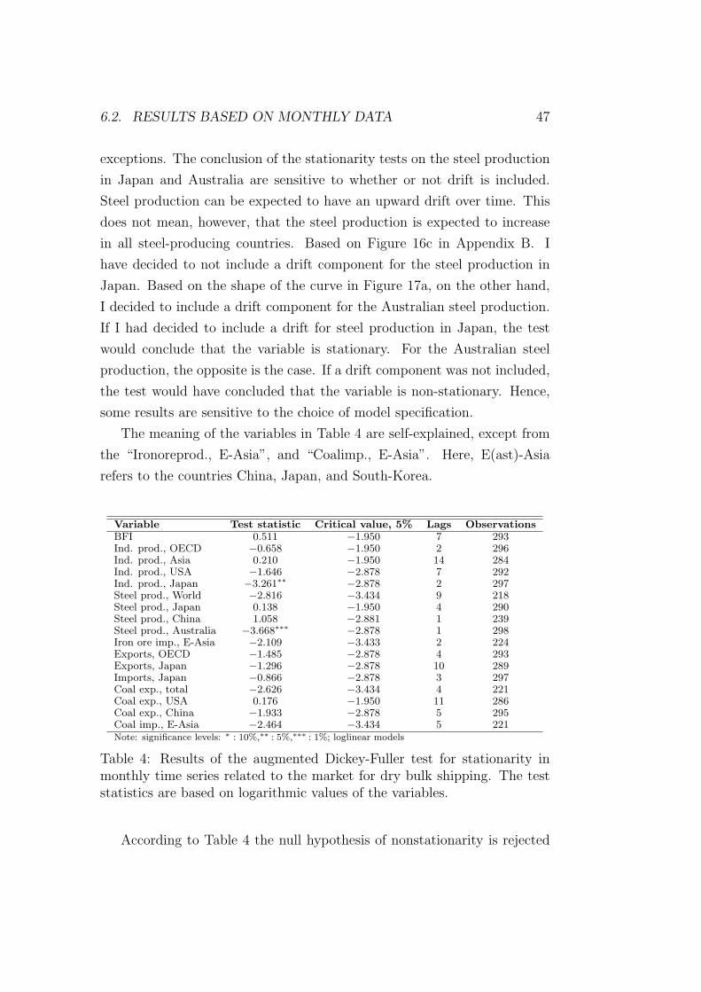
6.2. RESULTS BASED ON MONTHLY DATA 47
exceptions. The conclusion of the stationarity tests on the steel production
in Japan and Australia are sensitive to whether or not drift is included.
Steel production can be expected to have an upward drift over time. This
does not mean, however, that the steel production is expected to increase
in all steel-producing countries. Based on Figure 16c in Appendix B. I
have decided to not include a drift component for the steel production in
Japan. Based on the shape of the curve in Figure 17a, on the other hand,
I decided to include a drift component for the Australian steel production.
If I had decided to include a drift for steel production in Japan, the test
would conclude that the variable is stationary. For the Australian steel
production, the opposite is the case. If a drift component was not included,
the test would have concluded that the variable is non-stationary. Hence,
some results are sensitive to the choice of model specification.
The meaning of the variables in Table 4 are self-explained, except from
the “Ironoreprod., E-Asia”, and “Coalimp., E-Asia”. Here, E(ast)-Asia
refers to the countries China, Japan, and South-Korea.
Variable Test statistic Critical value, 5% Lags ObservationsBFI 0.511 −1.950 7 293Ind. prod., OECD −0.658 −1.950 2 296Ind. prod., Asia 0.210 −1.950 14 284Ind. prod., USA −1.646 −2.878 7 292Ind. prod., Japan −3.261∗∗ −2.878 2 297Steel prod., World −2.816 −3.434 9 218Steel prod., Japan 0.138 −1.950 4 290Steel prod., China 1.058 −2.881 1 239Steel prod., Australia −3.668∗∗∗ −2.878 1 298Iron ore imp., E-Asia −2.109 −3.433 2 224Exports, OECD −1.485 −2.878 4 293Exports, Japan −1.296 −2.878 10 289Imports, Japan −0.866 −2.878 3 297Coal exp., total −2.626 −3.434 4 221Coal exp., USA 0.176 −1.950 11 286Coal exp., China −1.933 −2.878 5 295Coal imp., E-Asia −2.464 −3.434 5 221Note: significance levels: ∗ : 10%,∗∗ : 5%,∗∗∗ : 1%; loglinear models
Table 4: Results of the augmented Dickey-Fuller test for stationarity inmonthly time series related to the market for dry bulk shipping. The teststatistics are based on logarithmic values of the variables.
According to Table 4 the null hypothesis of nonstationarity is rejected
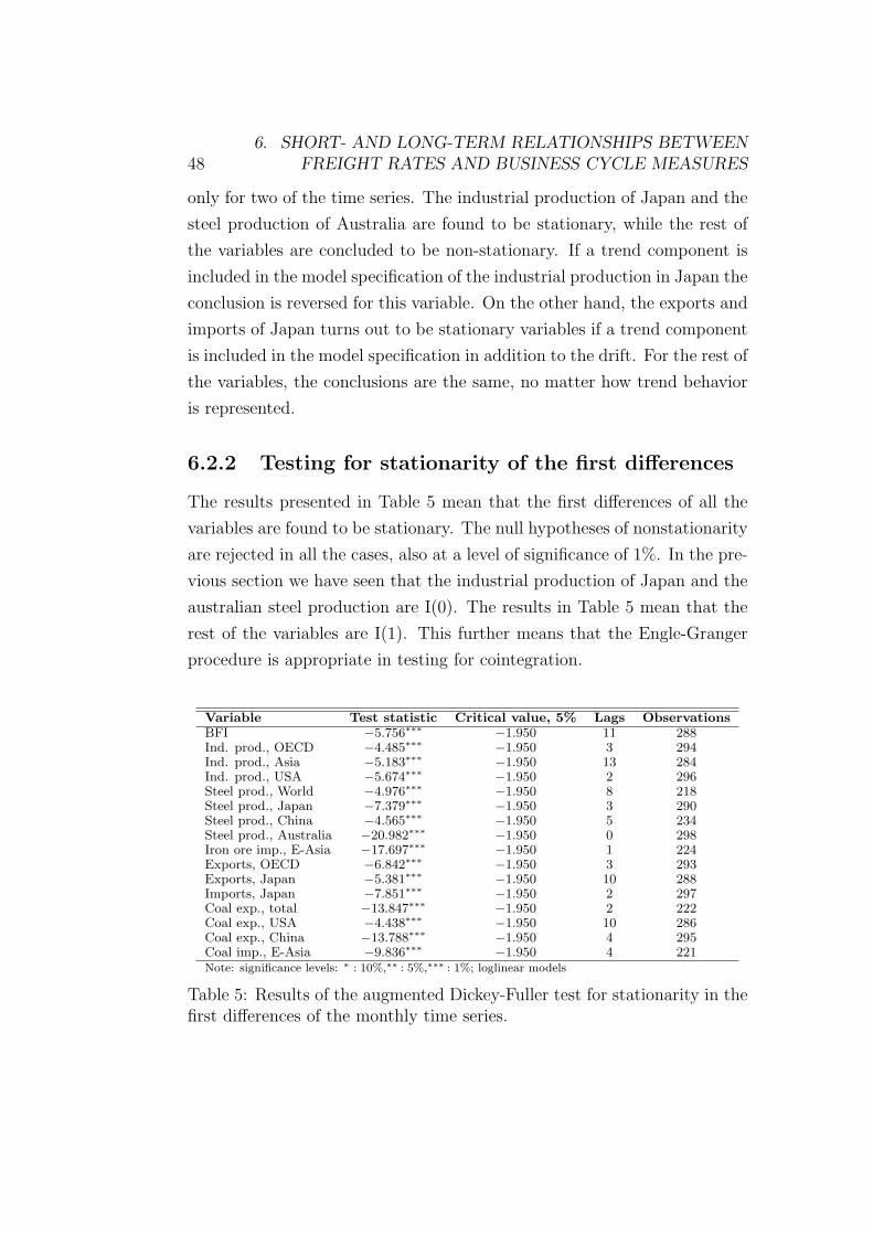
486. SHORT- AND LONG-TERM RELATIONSHIPS BETWEEN
FREIGHT RATES AND BUSINESS CYCLE MEASURES
only for two of the time series. The industrial production of Japan and the
steel production of Australia are found to be stationary, while the rest of
the variables are concluded to be non-stationary. If a trend component is
included in the model specification of the industrial production in Japan the
conclusion is reversed for this variable. On the other hand, the exports and
imports of Japan turns out to be stationary variables if a trend component
is included in the model specification in addition to the drift. For the rest of
the variables, the conclusions are the same, no matter how trend behavior
is represented.
6.2.2 Testing for stationarity of the first differences
The results presented in Table 5 mean that the first differences of all the
variables are found to be stationary. The null hypotheses of nonstationarity
are rejected in all the cases, also at a level of significance of 1%. In the pre-
vious section we have seen that the industrial production of Japan and the
australian steel production are I(0). The results in Table 5 mean that the
rest of the variables are I(1). This further means that the Engle-Granger
procedure is appropriate in testing for cointegration.
Variable Test statistic Critical value, 5% Lags ObservationsBFI −5.756∗∗∗ −1.950 11 288Ind. prod., OECD −4.485∗∗∗ −1.950 3 294Ind. prod., Asia −5.183∗∗∗ −1.950 13 284Ind. prod., USA −5.674∗∗∗ −1.950 2 296Steel prod., World −4.976∗∗∗ −1.950 8 218Steel prod., Japan −7.379∗∗∗ −1.950 3 290Steel prod., China −4.565∗∗∗ −1.950 5 234Steel prod., Australia −20.982∗∗∗ −1.950 0 298Iron ore imp., E-Asia −17.697∗∗∗ −1.950 1 224Exports, OECD −6.842∗∗∗ −1.950 3 293Exports, Japan −5.381∗∗∗ −1.950 10 288Imports, Japan −7.851∗∗∗ −1.950 2 297Coal exp., total −13.847∗∗∗ −1.950 2 222Coal exp., USA −4.438∗∗∗ −1.950 10 286Coal exp., China −13.788∗∗∗ −1.950 4 295Coal imp., E-Asia −9.836∗∗∗ −1.950 4 221Note: significance levels: ∗ : 10%,∗∗ : 5%,∗∗∗ : 1%; loglinear models
Table 5: Results of the augmented Dickey-Fuller test for stationarity in thefirst differences of the monthly time series.
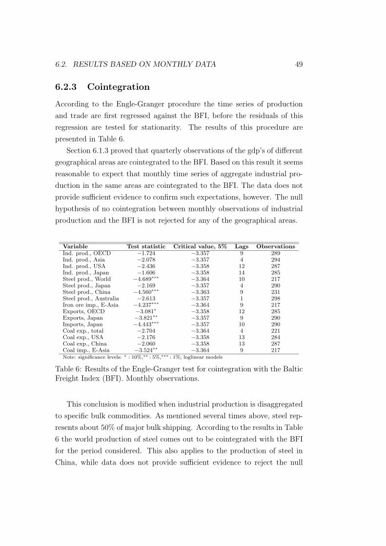
6.2. RESULTS BASED ON MONTHLY DATA 49
6.2.3 Cointegration
According to the Engle-Granger procedure the time series of production
and trade are first regressed against the BFI, before the residuals of this
regression are tested for stationarity. The results of this procedure are
presented in Table 6.
Section 6.1.3 proved that quarterly observations of the gdp’s of different
geographical areas are cointegrated to the BFI. Based on this result it seems
reasonable to expect that monthly time series of aggregate industrial pro-
duction in the same areas are cointegrated to the BFI. The data does not
provide sufficient evidence to confirm such expectations, however. The null
hypothesis of no cointegration between monthly observations of industrial
production and the BFI is not rejected for any of the geographical areas.
Variable Test statistic Critical value, 5% Lags ObservationsInd. prod., OECD −1.724 −3.357 9 289Ind. prod., Asia −2.078 −3.357 4 294Ind. prod., USA −2.436 −3.358 12 287Ind. prod., Japan −1.606 −3.358 14 285Steel prod., World −4.689∗∗∗ −3.364 10 217Steel prod., Japan −2.169 −3.357 4 290Steel prod., China −4.560∗∗∗ −3.363 9 231Steel prod., Australia −2.613 −3.357 1 298Iron ore imp., E-Asia −4.237∗∗∗ −3.364 9 217Exports, OECD −3.081∗ −3.358 12 285Exports, Japan −3.821∗∗ −3.357 9 290Imports, Japan −4.443∗∗∗ −3.357 10 290Coal exp., total −2.704 −3.364 4 221Coal exp., USA −2.176 −3.358 13 284Coal exp., China −2.060 −3.358 13 287Coal imp., E-Asia −3.524∗∗ −3.364 9 217Note: significance levels: ∗ : 10%,∗∗ : 5%,∗∗∗ : 1%; loglinear models
Table 6: Results of the Engle-Granger test for cointegration with the BalticFreight Index (BFI). Monthly observations.
This conclusion is modified when industrial production is disaggregated
to specific bulk commodities. As mentioned several times above, steel rep-
resents about 50% of major bulk shipping. According to the results in Table
6 the world production of steel comes out to be cointegrated with the BFI
for the period considered. This also applies to the production of steel in
China, while data does not provide sufficient evidence to reject the null
506. SHORT- AND LONG-TERM RELATIONSHIPS BETWEEN
FREIGHT RATES AND BUSINESS CYCLE MEASURES
hypothesis that steel production in Japan and Australia are cointegrated
with freight rates in shipping. The iron ore imports in China, Japan and
South-Korea is also found to be cointegrated with the BFI.
The results presented in Table 6 also means that some series of trade
flows are cointegrated with the BFI. The freight rates in shipping are for
instance cointegrated with the total exports from Japan at a 5% level of
significance and with total imports to Japan at a 1% level of significance.
This corresponds to the finding that the two series are highly correlated.
As pointed out above, Japan’s import is theoretically more satisfactory as
a potential determinant of dry bulk freight rates, since Japan’s exports are
mainly transported in liner shipping. The hypothesis of no cointegration
between the BFI and total exports from the OECD area is rejected at a
10% level of significance, and the total import of coal to China, Japan and
South-Korea is found to be cointegrated to the BFI.
It further follows from Table 6 that not all measures of trade flows and
production are found to be cointegrated to the BFI. Hence, there is no
unambiguous conclusion to the experiments with more disaggregated mea-
sures of activity than the gdp levels. The experiments prove, however, that
the freight rate in dry bulk shipping is at least related to some trade flows
and production measures through long-term equilibrium market forces. The
next section focuses more specifically on the dynamics in the relationship
between the variables that are found to be cointegrated.
6.2.4 Results based on Error Correction Models
Once again, let yt denote the BFI at time period t, while xt denotes the
variable representing a specific production measure or trade flow, and et−1 is
the estimated error terms from the corresponding cointegration regression.
Consider first the world steel production. The error correction model in
logs is estimated as a reduced form, and the OLS regression then gives the
following result:
∆(ln yt) = − 0.002
(0.009)
+ 2.818
(0.404)
∆(lnxSteel, worldt )− 0.063
(0.023)
eSteel, worldt−1 (17)

6.2. RESULTS BASED ON MONTHLY DATA 51
Hence, both the effect of the error correction term and the contempora-
neous effect of a change in the exogenous variable, ∆ lnxSteel, worldt , are
estimated to influence the freight rates in dry bulk significantly. The corre-
sponding P -values are 0.000 and 0.008, respectively, and the results mean
that:
• a 1% change in the growth of world steel production immediately
causes a 2.8% change in the growth rate of the BFI
• about 6.3% of the deviation from the equilibrium between the BFI
and the world steel production will be corrected in the subsequent
month
This estimation is based on 227 observations, and the model explains about
19.5% of the variation in the logarithm of the changes in dry bulk freight
rates (R2adj ≈ 0.1951).
Now, turn to the other variables that proved to be cointegrated with
the BFI. The estimation results following from an error correction model
specification are as follows:
∆(ln yt) = − 0.002
(0.009)
+ 0.700
(0.266)
∆(lnxSteel, Chinat )− 0.054
(0.021)
eSteel, Chinat−1
(18)
∆(ln yt) = 0.004
(0.100)
+ 0.202
(0.097)
∆(lnxIron ore, E-Asiat )− 0.054
(0.022)
eIron ore, E-Asiat−1
(19)
∆(ln yt) = 0.005
(0.008)
+ 0.276
(0.176)
∆(lnxExports, Japant )− 0.030
(0.020)
eExports, Japant−1
(20)
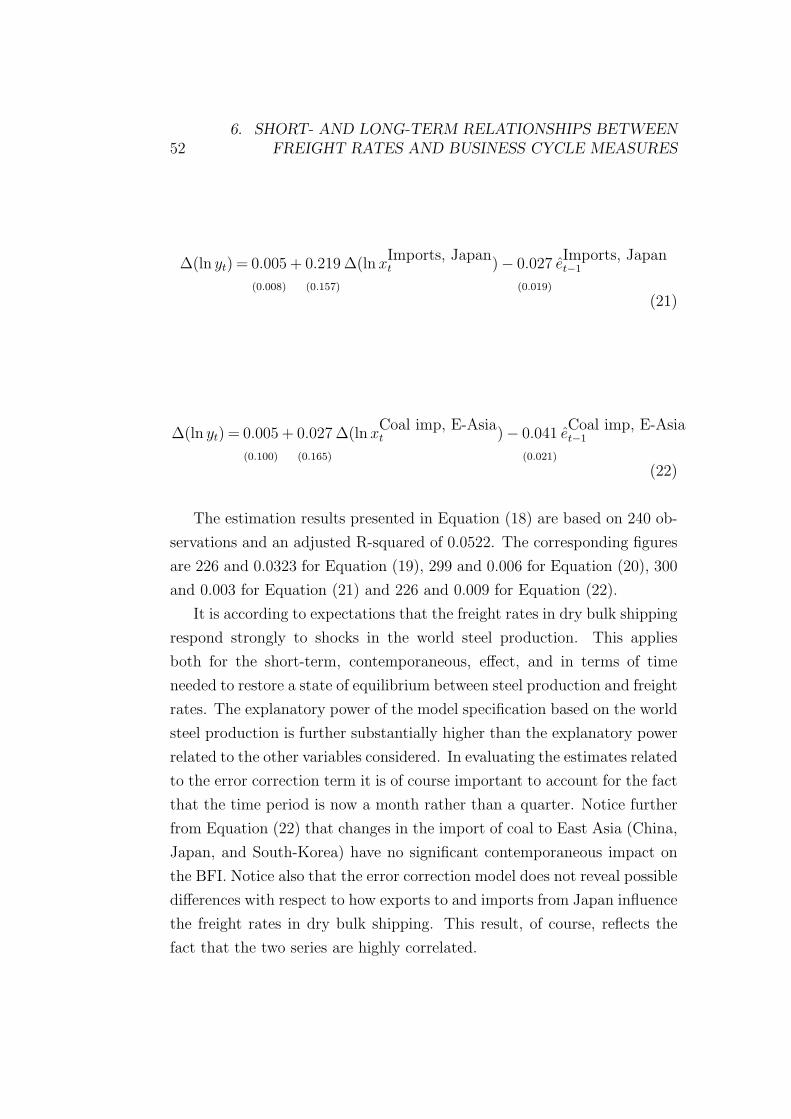
526. SHORT- AND LONG-TERM RELATIONSHIPS BETWEEN
FREIGHT RATES AND BUSINESS CYCLE MEASURES
∆(ln yt) = 0.005
(0.008)
+ 0.219
(0.157)
∆(lnxImports, Japant )− 0.027
(0.019)
eImports, Japant−1
(21)
∆(ln yt) = 0.005
(0.100)
+ 0.027
(0.165)
∆(lnxCoal imp, E-Asiat )− 0.041
(0.021)
eCoal imp, E-Asiat−1
(22)
The estimation results presented in Equation (18) are based on 240 ob-
servations and an adjusted R-squared of 0.0522. The corresponding figures
are 226 and 0.0323 for Equation (19), 299 and 0.006 for Equation (20), 300
and 0.003 for Equation (21) and 226 and 0.009 for Equation (22).
It is according to expectations that the freight rates in dry bulk shipping
respond strongly to shocks in the world steel production. This applies
both for the short-term, contemporaneous, effect, and in terms of time
needed to restore a state of equilibrium between steel production and freight
rates. The explanatory power of the model specification based on the world
steel production is further substantially higher than the explanatory power
related to the other variables considered. In evaluating the estimates related
to the error correction term it is of course important to account for the fact
that the time period is now a month rather than a quarter. Notice further
from Equation (22) that changes in the import of coal to East Asia (China,
Japan, and South-Korea) have no significant contemporaneous impact on
the BFI. Notice also that the error correction model does not reveal possible
differences with respect to how exports to and imports from Japan influence
the freight rates in dry bulk shipping. This result, of course, reflects the
fact that the two series are highly correlated.
6.3. CRITICAL REMARKS ON THE EMPIRICAL RESULTS 53
6.3 Critical remarks on the empirical
results
It can be argued that the error correction models in Section 6.1.4 and Sec-
tion 6.2.4 are too basic to capture the true relationships between the freight
rates and the various business cycle measures. The adjusted R-squared,
which represents the explanatory power of the models, ranges from less
than 1% to about 20%. Hence, the volatility in the freight rates is only to
a modest degree explained by the models.
To increase the explanatory power it is possible to include explicitly
components influencing the demand and supply in the market for dry bulk
shipping. Recall that the ambition of this thesis is to study the relationship
between business cycles and freight rates in dry bulk shipping, rather than
developing an econometric model attempting to explain all the volatility of
the freight rates. This does not mean that additional variables are irrele-
vant, however, for instance to avoid problems related to omitted variables.
The demand for sea transport was represented by measures of gdp, pro-
duction and trade flows in the preceding sections. Based for instance on
Stopfords (2009, p. 139-149) five key factors influencing the demand for
sea transport, it is of course possible to specify other demand factors in the
regressions. According to Stopford (Stopford, 2009, p. 140), the business
cycle is “the most important cause of short-term fluctuations in seaborne
trade and ship demand”. I will not enter into details on other demand
related variables that could be included in the model.
The major driver of short-term variation in freight rates is expected to
be the demand, as there is a time lag in the adjustment of the supply. Still,
supply factors also have an impact on the determination of freight rates. It
is beyond the scope of this thesis to take such factors explicitly into account
in the analysis, but I will briefly mention some relevant aspects. In Section
3.2 there was a discussion of the supply of sea transport. In order to fully
control for the supply of sea transport, one needs data on the size of the
fleet as well as of the fleet utilization. Data on the size of the fleet are
easily available, see Figures 20a and 20b in Appendix B for time series on
546. SHORT- AND LONG-TERM RELATIONSHIPS BETWEEN
FREIGHT RATES AND BUSINESS CYCLE MEASURES
the fleet size. Fleet utilization, on the other hand, must be calculated based
on factors such as waiting time in port and operating speed. This is a time
consuming and complex task, and if the calculations are not done properly
the results may confuse more than they help.
Shipowners investment decisions are of course also important in explain-
ing the supply of shipping services. Most of the literature considers exoge-
nous demand factors to be the main determinants of freight rates. Accord-
ing to Randers and Goluke (2007), however, shipowners are to a large degree
responsible for the high volatility in the market: “In our view ship owners
contribute to their own difficulties. The shipping community creates the
cyclicality and adds significantly to the volatility of the business environ-
ment through their own investment and allocation decisions. We call this
perspective the ”self-infliction view” ”(Randers and Goluke (2007). Accord-
ing to Randers and Goluke (2007) the rationale for this behaviour is that
increased volatility improves the chances of making fortunes in shipping.
Analogously, Stopford (2009) claims that the risk profile for investors in
shipping may differ systematically from the risk profile of investors in other
sectors, being less risk averse.
It is possible to incorporate hypotheses of investments decisions, for
instance by introducing adaptive expectations of some kind, based on the
observed development of the freight rates in previous periods. Another
supply factor that may be explicitly included is the bunker price. There
is a discussion of the effects of an increased price of bunker fuel in Section
7.3. Studying the short and long-term relationship between the supply of
sea transport and freight rates in dry bulk shipping is, however, beyond the
scope of this thesis. Hence, I will not enter into a discussion of how such
factors could be made operational in a model formulation. I have chosen to
keep the model simple, rather than experimenting with additional factors
influencing the supply and demand in shipping markets. If such factors
were included I also had to deal with problems related to multicollinearity
and identification, in addition to testing for stationarity etc. This is left for
future research.
In Section 6.1.1 and Section 6.2.1 the freight rates in dry bulk shipping

6.3. CRITICAL REMARKS ON THE EMPIRICAL RESULTS 55
were found to be non-stationary. These results are in line with most empiri-
cal studies on stationarity of freight rates (see for example Berg-Andreassen
(1996) or Veenstra and Frandes (1997)). There are, however, some empirical
studies that reach the opposite conclusion. According to Tvedt (2003), the
freight rates in dry bulk shipping become stationary if they are converted
from US dollars to Japanese yen. He argues that the main driver of the dry
bulk shipping industry is the Japanese economy. Therefore, he claims, it
is more appropriate to study the freight rates converted to Japanese yen.
Tvedt (2003) uses data from 1985 - 1999. In the 2000s, China has strength-
ened its position in dry bulk shipping, and it can be argued that the Chinese
economy now is the main driver of the industry.
The most commonly used test for stationarity is the traditional Dickey-
Fuller test (Dickey and Fuller, 1979). This test was used in Section 6
above, as in most of the empirical research on stationarity of freight rates
in shipping. The traditional Dickey Fuller test is a linear stationarity test.
Koekebakker et al. (2006) claim that there are empirical evidence and theo-
retical support of a non-linear behaviour of the spot freight rates. When the
spot freight rates are tested for stationarity with a nonlinear version of the
(Augmented) Dickey-Fuller test, Koekebakker et al. (2006) found that the
freight rates both in dry bulk shipping and in tanker shipping are nonlinear
stationary. They also claim that maritime economic theory supports this
finding. The argument is that over time it is not sustainable with extremely
high or extremely low freight rates, and hence, ”the freight rate cannot ex-
hibit the asymptotically explosive behaviour implied by a non-stationary
process” (Koekebakker et al. 2006). They further argue that the standard
conclusion of non-stationary freight rates is due to the weak power of the
stationarity tests being used. Still, I have chosen to proceed according to
the traditional approach. This controversy of stationarity is, however, an
example of a discussion that I would like to enter more thoroughly into if I
had more time available for this thesis.
567. INTERPRETING RESULTS IN TERMS OF A COMPETITIVE
EQUILIBRIUM MODEL
7 Interpreting results in terms of a
competitive equilibrium model
According to the empirical results presented in Section 6 there is an equi-
librium relationship between freight rates in shipping and some business
cycle measures. The error correction model further provided results on the
dynamics involved in this relationship, distinguishing between the contem-
poraneous effect of a demand shock, and the time it takes to restore an
equilibrium situation. The next challenge is to interpret those results in
terms of the partial competitive equilibrium model presented in Section 3.
The discussion to follow focuses on alternative scenarios of demand and sup-
ply shocks, as well as on possible short- and long-term dynamics following
from such shocks. As a convenient simplifying assumption the illustrations
ignore the possibility that freight rates reach a level corresponding to the
elastic part of the demand curve, see Figure 5.
7.1 A general demand shock
The results presented in Section 6.1 proved that
• all the quarterly time series of alternative gdp-measures are non-
stationary; I(1)
• the first differences of those time series are stationary, I(0)
• all the tested quarterly gdp-measures are cointegrated with the Baltic
Freight Index
This means that the relationship between the business cycle situation and
the freight rates in dry bulk shipping tend to converge towards a long-
term equilibrium solution. There are several possible reasons for such an
equilibrium relationship. As pointed out in Section 5.2 one of the variables
can for example depend on the other, or they may both depend on the
same exogenous factors. In the relevant example it is natural to consider
the freight rates in shipping to depend on the business cycle situation.
7.1. A GENERAL DEMAND SHOCK 57
Changes in the business cycle situation appear as exogenous demand shocks,
followed by some forces pulling the market for shipping services towards a
new equilibrium solution.
The error correction model is more specific both on the contemporaneous
effect of a demand shock, and on the dynamics towards a new equilibrium
solution. Consider for example the results from the error correction model
based on the gdp of the OECD as a measure of the business cycle situation.
Recall from Section 6.1.4 that the estimated elasticity of freight rates with
respect to changes in the gdp of the OECD is about 15.2. According to the
shape of the highly nonlinear supply curve a demand shock will influence
strongly on the freight rates especially in situations where the supply is close
to its capacity limit. Hence, the high elasticity estimate indicates that the
market has been operating close to its capacity limit in the period covered
by the data.
The nonlinear character of the supply curve is of course a challenge if
the results from the error correction model are used to predict the contem-
poraneous effect of a demand shock. The prediction has to be based on an
assumption of the capacity situation of the shipping market. The elasticity
estimate is not reliable for prediction purposes if the capacity situation in
the prediction period differs from the situation in the period covered by the
data.
Assume that point A in Figure 8 corresponds to a long-term equilibrium
solution, where the freight rate equals the average cost of dry bulk ship-
ping. Hence, the profits are equal to zero, and there are no incentives for
shipowners to exit from the market, nor to enter the market.
The system is next disturbed by a positive demand shock, represented
by the shift from D0 to D1 in Figure 8. The immediate effect is to increase
the freight rates from P0 to P1, while the freight volumes increase from
Q0 to Q1. This increased freight volume is explained by a more intensive
utilization of the fleet, see Section 3.2 for more details on how vessels can
be more intensively utilized.
There are reasons to believe that the short-term equilibrium solution A
will not be stable, however. The freight rate P1 is substantially higher than
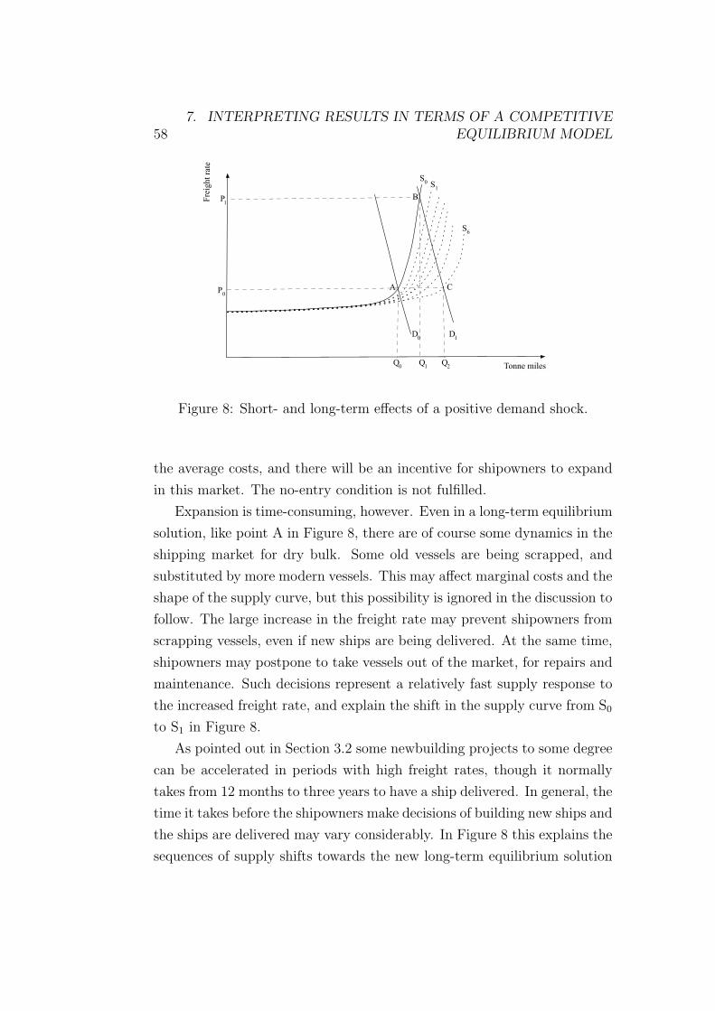
587. INTERPRETING RESULTS IN TERMS OF A COMPETITIVE
EQUILIBRIUM MODEL
Fre
ight
rate
Tonne miles
A
0D
1D
0P
P B1
0S
1S
C
6S
0Q
1Q
2Q
Figure 8: Short- and long-term effects of a positive demand shock.
the average costs, and there will be an incentive for shipowners to expand
in this market. The no-entry condition is not fulfilled.
Expansion is time-consuming, however. Even in a long-term equilibrium
solution, like point A in Figure 8, there are of course some dynamics in the
shipping market for dry bulk. Some old vessels are being scrapped, and
substituted by more modern vessels. This may affect marginal costs and the
shape of the supply curve, but this possibility is ignored in the discussion to
follow. The large increase in the freight rate may prevent shipowners from
scrapping vessels, even if new ships are being delivered. At the same time,
shipowners may postpone to take vessels out of the market, for repairs and
maintenance. Such decisions represent a relatively fast supply response to
the increased freight rate, and explain the shift in the supply curve from S0
to S1 in Figure 8.
As pointed out in Section 3.2 some newbuilding projects to some degree
can be accelerated in periods with high freight rates, though it normally
takes from 12 months to three years to have a ship delivered. In general, the
time it takes before the shipowners make decisions of building new ships and
the ships are delivered may vary considerably. In Figure 8 this explains the
sequences of supply shifts towards the new long-term equilibrium solution
7.2. A DEMAND SHOCK IN A SEPARATE SUBMARKET 59
in point C. Each supply curve represents the situation in a specific quarter.
According to the results following from the error correction model about
16% of the deviation from the equilibrium level between the BFI and the gdp
of the OECD will be corrected in the subsequent quarter. This means that
it takes about 6 quarters to get back to a stable equilibrium solution, where
the freight rate reaches the level prior to the demand shock. As the freight
rate is successively reduced, the incentives for new deliveries comes to an
end, until a new equilibrium is reached, with a balance between deliveries
and scrapping of vessels.
7.2 A demand shock in a separate
submarket
As pointed out in Section 2.1 and illustrated in Figure 1 there is a high
degree of covariation between the freight rates of different submarkets of dry
bulk shipping. The literature also provides arguments that shocks in one
submarket tend to spread to other submarkets, and that the freight market
in general can be considered to be integrated (see for instance Strandenes
1981). At the same time, however, there may be substantial differences
between the freight rates of different submarkets at a specific point in time,
as pointed out for instance by Laulajainen (2006). In this section such
observations are interpreted in an analytical framework.
A worldwide economic upturn is expected to affect the market for dry
bulk shipping in general. It is of course possible, however, that the increased
demand is restricted to a specific geography and/or to a specific commodity.
In such a case the demand for shipping services is increased for a few routes,
and left unchanged in the rest of the system. One example may be an
increased Chinese steel production. According to the results presented in
Section 6.2.3 the Chinese steel production is cointegrated to the freight rates
in dry bulk shipping. The results from the error correction model means
that an increased production has a significant contemporaneous effect on
the freight rate, and that about 5.4% of the deviation from the equilibrium

607. INTERPRETING RESULTS IN TERMS OF A COMPETITIVE
EQUILIBRIUM MODEL
between the BFI and the Chinese steel production will be corrected in the
subsequent month. This further means that it will take about 18 months
to restore the equilibrium solution after a shock has occurred.
Figure 9 offers an illustration of such a scenario. The figure is based on
the assumption that only submarket A is affected initially. This submarket
is represented by the left part of the figure, while the rest of the market for
dry bulk shipping is represented by the right part, denoted as submarket
B. The analysis starts from a long-term equilibrium solution where the
freight rate (P0) is assumed to equal the average cost of dry bulk shipping,
and equal in different submarkets. The system is then disturbed by an
exogenously increased demand in submarket A, represented by the shift
from DA0 to DA
1 in the left part of the figure.
Fre
ight
rate
Tonne miles
0P
Fre
ight
rate
Tonne miles0
QA
1P
2P
1Q
A
2Q
A0
QB
2Q
B
3Q
A
1D
A
0D
A
0S
A 0S
B
S1
A 1S
B
S18
A
Figure 9: Short- and long-term effects of a positive demand shock in aspecific submarket.
The contemporaneous effect of the demand shift is to raise the freight
rate in the relevant submarket substantially, from P0 to P1 in the figure.
According to the results in Section 6.2.4 the contemporaneous effect of an
increased steel production in China is represented by an elasticity of 0.7, see
Equation (18). This relatively low elasticity apparently does not correspond
to the large contemporaneous increase of the freight rate in Figure 9. Recall,
however, that the price variable used in the error correction model is a
7.2. A DEMAND SHOCK IN A SEPARATE SUBMARKET 61
freight rate index, while the freight rates in Figure 9 applies for the specific
submarkets. Hence, the fact that an increase in the Chinese steel production
is estimated to have a moderate impact on the Baltic Freight Index does
not mean that the contemporaneous effect on the freight rate of specific
routes is moderate.
The increased freight rate from P0 to P1 in Figure 9 of course refers to
a very short-term time perspective, for which the capacity on the specific
route is more or less given, corresponding to a given number of vessels oper-
ating here. Extending the time perspective, however, means that a freight
rate level of P1 does not represent an equilibrium solution. This freight rate
is substantially higher than the average cost of dry bulk shipping, and the
law of one price for homogeneous services (shipping) is violated. Hence,
shipowners may increase their profits by moving their vessels to routes
transporting steel produced in China. This explains the positive supply
curve shift from SA0 to SA
1 in the left part of Figure 9, and the negative
shift from SB0 to SB
1 in the right part of the figure. In the medium-term
equilibrium solution corresponding to a freight rate of P2 the potential for
profit by switching between submarkets is exhausted.
The solution with a freight rate of P2 and transportation volumes of
QA2 and QB
2 does not meet the no-entry condition, and hence is no long-
term equilibrium solution. The return on the shipowners capital is higher
than the normal return in the market, and the fleet should be expected
to expand until the point where there is no more room for supernormal
profits. According to the results based on the error correction model, this
process will take about 18 months, and it goes on until the position of the
new supply curve is SA18 in Figure 9. The supply curve in submarket B will
eventually shift back to its initial position, from SB1 to SB
0 .
In the long-term equilibrium solution in Figure 9 the freight rate has
returned to its initial level. The distribution of transportation volumes
and capacity between the different submarkets has changed, however. The
transportation volume in submarket B is unaffected by the demand shock
in submarket A, in a long-term time perspective, but the transportation
volumes in submarket A has increased. The increased QA can be explained
627. INTERPRETING RESULTS IN TERMS OF A COMPETITIVE
EQUILIBRIUM MODEL
as the result of a sequence of adjustments. First, the increase from QA0
QA1 is explained by a higher utilization of the initial fleet. The increased
transportation volume from QA1 to QA
2 reflects the fact that vessels are at-
tracted from other submarkets, while the increase towards QA3 is a response
of gradual expansions of the fleet.
The process leading from the initial to the final equilibrium solution in
Figure 9 represents a reasonable explanation of the empirical finding that
the time series of Chinese steel production is cointegrated to the freight rate
in dry bulk shipping.
The analysis in this section is based on the assumption that the long-
term equilibrium freight rates will be equal in the separate submarkets. As
pointed out in Section 3.1, however, there are limits to substitution and
integration. Adland and Strandenes (2004) for instance claim that there
will exist a positive freight rate differential between a Suezmax tanker and
a VLCC trading on the same route, due to economies of scale offered by
the VLCC. The possibility of persistent differentials is not accounted for in
the analysis above.
7.3 Effects of an increased price of bunker
fuel
The price of bunker fuel probably is the single factor that has the strongest
influence on short-term fluctations in the supply of sea transport. Most of
the commercial fleet is operating on bunker fuel, but there are several types
of fuel used. According to Wang et al. (2010), bunker fuel is a residual
fuel which originally was defined as the liquid that was left after removing
the most valuable products in the petroleum distillation process. Wang et
al. (2010) further write that the two basic grades of bunker fuel are IFO
180 and IFO 380. IFO 380 represents 60% of the world volume in bunkers,
while IFO 180 and some other grades represent 30%. 10% of the world
volume in bunkers is in Marine Diesel Oil (Alizadeh et al., 2004).
The price of each grade further varies between ports. I have tested time
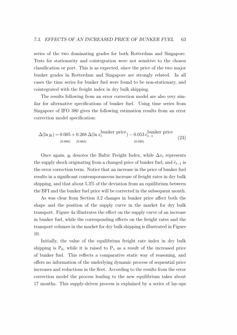
7.3. EFFECTS OF AN INCREASED PRICE OF BUNKER FUEL 63
series of the two dominating grades for both Rotterdam and Singapore.
Tests for stationarity and cointegration were not sensitive to the chosen
classification or port. This is as expected, since the price of the two major
bunker grades in Rotterdam and Singapore are strongly related. In all
cases the time series for bunker fuel were found to be non-stationary, and
cointegrated with the freight index in dry bulk shipping.
The results following from an error correction model are also very sim-
ilar for alternative specifications of bunker fuel. Using time series from
Singapore of IFO 380 gives the following estimation results from an error
correction model specification:
∆(ln yt) = 0.005
(0.008)
+ 0.268
(0.063)
∆(lnxbunker pricet )− 0.053
(0.020)
ebunker pricet−1 (23)
Once again, yt denotes the Baltic Freight Index, while ∆xt represents
the supply shock originating from a changed price of bunker fuel, and et−1 is
the error correction term. Notice that an increase in the price of bunker fuel
results in a significant contemporaneous increase of freight rates in dry bulk
shipping, and that about 5.3% of the deviation from an equilibrium between
the BFI and the bunker fuel price will be corrected in the subsequent month.
As was clear from Section 3.2 changes in bunker price affect both the
shape and the position of the supply curve in the market for dry bulk
transport. Figure 4a illustrates the effect on the supply curve of an increase
in bunker fuel, while the corresponding effects on the freight rates and the
transport volumes in the market for dry bulk shipping is illustrated in Figure
10.
Initially, the value of the equilibrium freight rate index in dry bulk
shipping is P0, while it is raised to P1 as a result of the increased price
of bunker fuel. This reflects a comparative static way of reasoning, and
offers no information of the underlying dynamic process of sequential price
increases and reductions in the fleet. According to the results from the error
correction model the process leading to the new equilibrium takes about
17 months. This supply-driven process is explained by a series of lay-ups
647. INTERPRETING RESULTS IN TERMS OF A COMPETITIVE
EQUILIBRIUM MODEL
and vessel scrappings, reflecting the reduced profit resulting from increased
operating costs. Eventually, a new stable equilibrium is reached where the
freight rate has increased to a level, P1 in Figure 10, where shipowners earn
no supernormal profits.
Fre
ight
rate
Tonne miles
D
S1
S0
P0
P1
Figure 10: Effects of an increased price of bunker fuel.
It is worth mentioning that in addition to influencing the supply of sea
transport there is another reason why the bunker price may be cointegrated
with the BFI. Bunker is, as discussed above, a petroleum product, and hence
the price of bunkers is expected to be strongly correlated with the oil price.
According to Mork (1994) the oil price is correlated with business cycles. In
Section 6 it was proven that the BFI is cointegrated with several measures
of business cycles. Hence, the bunker price and the BFI can be argued to
depend on the same exogenous factors.
7.4 The dramatic recent fall in freight rates
So far in this thesis, I have not explicitly addressed the role of expectations.
Studying the role of expectations is a complex task. It can be argued that
both the supply and the demand for sea transport is a result of expectations.
7.4. THE DRAMATIC RECENT FALL IN FREIGHT RATES 65
If shipowners expect the freight rates to be increasing in the coming period,
they tend to increase their fleet.
The role of expectations in shipping markets can be studied by looking
at the second-hand price of vessels. According to Strandenes (1986), the
price of second-hand vessels depend on expectations about the future of the
shipping industry worldwide. Merikas et al. (2008) studied the relationship
between the price on second-hand vessels (SH) and the newbuilding price
(NP) for tankers by studying the ratio SH/NP. Merikas et al. (2008) found
that the SH/NP price ratio is positively related to the freight rate. This
result is not very surprising. According to Stopford (2009, p. 639) it takes
12 months to 3 years to have a new vessel delivered. A second-hand vessel
can, on the other hand, be delivered on a relatively short notice, as it is
already in the market.
The value of a vessel is its discounted expected future income. If freight
rates are very high shipowners want ships delivered as soon as possible
in order to exploit the high freight rates. Hence, second-hand vessels are
then priced relatively high compared to newbuildings. Assume for instance
a period with high but falling freight rates. The value of a second-hand
vessel delivered today, with 20 years left before scrapping, may then exceed
the value of a newbuilding delivered in 5 years, even if the new ship will be
operating for 25 years. Merikas et al. (2008) also pointed out that when
the freight rate falls, the SH/NP price ratio drops not only because of the
reduced price on second-hand vessels. The shipowners also tend to believe
that there will be a recovery of the market in the future, and hence order
new vessels based on this expectation. As mentioned Merikas et al. (2008)
studied the market for tankers, but there is no reason to believe the results
would differ for bulk vessels.
It can be argued that expectations depend on the recent development
in demand and freight rates. In a period where both the demand and the
freight rates increased substantially, shipowners expect this development to
continue, or at least the market demand to stabilize at a very high level.
As a response, new ships are ordered, leading to an increased fleet. As
discussed in Section 3.2 this causes a shift of the supply curve towards the
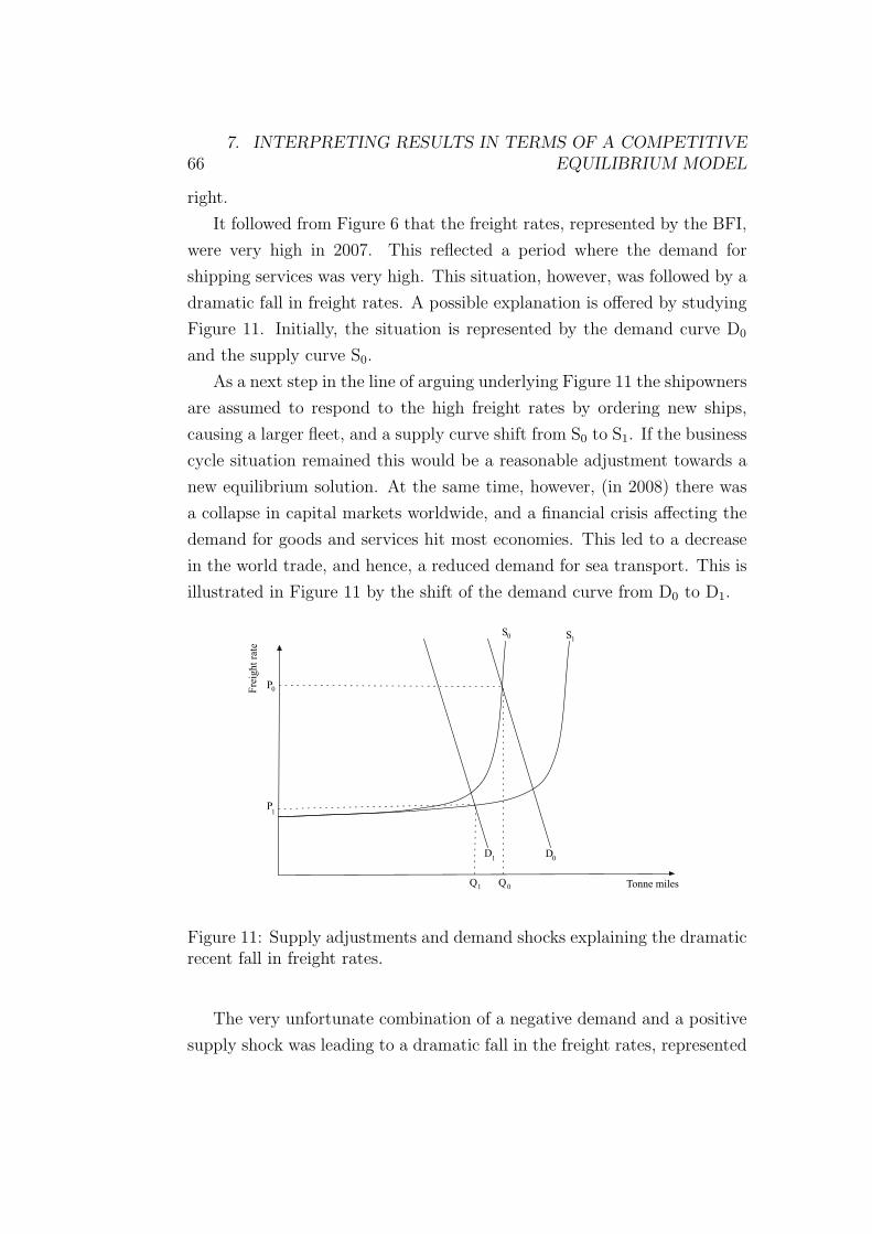
667. INTERPRETING RESULTS IN TERMS OF A COMPETITIVE
EQUILIBRIUM MODEL
right.
It followed from Figure 6 that the freight rates, represented by the BFI,
were very high in 2007. This reflected a period where the demand for
shipping services was very high. This situation, however, was followed by a
dramatic fall in freight rates. A possible explanation is offered by studying
Figure 11. Initially, the situation is represented by the demand curve D0
and the supply curve S0.
As a next step in the line of arguing underlying Figure 11 the shipowners
are assumed to respond to the high freight rates by ordering new ships,
causing a larger fleet, and a supply curve shift from S0 to S1. If the business
cycle situation remained this would be a reasonable adjustment towards a
new equilibrium solution. At the same time, however, (in 2008) there was
a collapse in capital markets worldwide, and a financial crisis affecting the
demand for goods and services hit most economies. This led to a decrease
in the world trade, and hence, a reduced demand for sea transport. This is
illustrated in Figure 11 by the shift of the demand curve from D0 to D1.
Fre
ight
rate
Tonne miles
S1S0
P0
D0
D1
P1
Q1 Q0
Figure 11: Supply adjustments and demand shocks explaining the dramaticrecent fall in freight rates.
The very unfortunate combination of a negative demand and a positive
supply shock was leading to a dramatic fall in the freight rates, represented
67
by the reduction from P0 to P1 in Figure 11. As illustrated in the figure the
combination of the shifts in the demand and the supply curve also leads to
a reduction in tonne miles transported. In a short-term time perspective
this leads to a low utilization of the fleet. Starting from an equilibrium
represented by the intersection of D1 and S1, moderate shifts in the demand
curve will not result in large changes in the freight rate. Even an increased
demand back to the initial level represented by the curve D0 would just have
a modest impact on the freight rate. As a next response the number of lay-
ups can be expected to increase, before the shipowners may decide to scrap
their oldest and least efficient ships. Eventually a new equilibrium arises
with freight rates approximately equal to marginal and average operating
costs and a normal degree of fleet utilization.
Once again there will of course be lags in the adjustments of the fleet.
This is another example of a complex and time-consuming mechanism ex-
plaining why business cycle measures tend to be cointegrated with the
freight rate, and why the results from the error correction model suggest a
slow adjustment towards a new equilibrium solution.
8 A summary of results and some
concluding remarks
The empirical section of this thesis was focusing on short- and long-term
relationships between freight rates in dry bulk shipping and alternative
measures representing the demand for dry bulk shipping services. As a
first reasonable hypothesis the demand for shipping is assumed to be pos-
itively dependent on trade flows, which further are assumed to reflect the
business cycle situation. Next, business cycles are represented by quarterly
observations of the gross domestic product. The shipping market effects
of a demand shock may depend on where the shock originates. Hence, the
analysis accounts for gdp variations for some geographies/countries that are
potentially important in studying markets for dry bulk shipping.
All quarterly variables, the gdp of OECD, USA, Japan, and China, are

688. A SUMMARY OF RESULTS AND SOME CONCLUDING
REMARKS
found to be non-stationary, as is the relevant time series for the Baltic
Freight Index. Fortunately, both the BFI and the gdp variables were found
to be integrated of order 1, I(1), making them appropriate for the Engle-
Granger procedure in testing for cointegration. This procedure further led
to the conclusion that all the alternative business cycle measures are coin-
tegrated with the BFI.
This important empirically based conclusion further means that there is
an equilibrium relationship between the business cycle and the freight rates
in dry bulk shipping. Hence, demand shocks caused by a changed business
cycle situation initiate forces pulling the dry bulk shipping market towards
a new equilibrium. It further follows from the observed time series that the
relationship between the BFI and the alternative gdp indicators converge
towards a long-term equilibrium solution.
The presence of cointegration justifies the use of an error correction
model, and which allows for a short- and medium term analysis of demand
shocks. The contemporaneous effect of a change in the gdp is found to be
larger for OECD as a whole than for each of the three countries separately.
This supports the hypothesis that the gdp of OECD is a more appropriate
measure of the worldwide business cycle. The results also provide evidence
of the increasingly important position of China in the market for dry bulk
shipping over recent years. Finally, the results offer information on the
dynamics of the process towards a new long-term equilibrium after a shock
has occurred. About 12% of the deviation from the equilibrium between the
BFI and the gdp of OECD is predicted to be corrected in the subsequent
quarter. For the gdp of China the corresponding estimate is 31%.
The results following from monthly data on more disaggregated vari-
ables are somewhat more ambiguous. The disaggregation refers to various
combinations of geographical areas and trade or production of different bulk
commodities. Most of the time series were found to be non-stationary, and
all the corresponding variables were integrated of order 1. Data does not,
however, provide sufficient evidence that all the variables are cointegrated
to the BFI. Still, the experiments prove that the freight rate in dry bulk
shipping is at least related to some trade flows and production measures
69
through long-term equilibrium market forces. This applies, for instance, to
the world steel production and the steel production in China.
Results based on the error correction model are also ambiguous. For
most of the variables the term representing the contemporaneous effect did
not come out to be significantly different from zero. This did not apply for
the world steel production, however. The freight rates in dry bulk shipping
were found to respond strongly to shocks in the world steel production.
According to the estimate of the error correction term, it takes about 18
months to restore a state of long-term equilibrium following from a shock in
the world steel production. The time needed for adjustments is estimated
to be longer for the other variables that are cointegrated with the BFI, but
the estimates are still within a sensible range of values.
An ambition of this thesis has been to interpret the empirical results
in terms of a competitive equilibrium model. Considering the dynamic
adjustments incorporated in the econometric approach, such an interpreta-
tion ideally calls for a dynamically formulated modelling framework. The
competitive equilibrium model that is used in the analysis is basically con-
structed for comparative static analyses. By introducing some ad hoc dy-
namics, however, I think that the model is appropriate for explaining both
the results from the cointegration tests and the results based on the error
correction modelling approach.
The theoretical interpretation of results is based on case studies. The
study of a general demand shock is motivated to explain both the con-
temporaneous shipping market effect of a world economy upturn, and the
competitive forces bringing the market back to a state of long-term equilib-
rium. Next, the study of a demand shock in a separate submarket focused
on the interrelationship between submarkets in shipping. The substitution
of vessels causes integrated markets, and competition contributes to a so-
lution where the law of one price holds in markets for dry bulk shipping.
This competition of course also involves variations in the fleet, including
new deliveries of ships, or lay-ups and scrapping in the case of less opti-
mistic market prospects.
As another case study, cointegration tests, the error correction model,

708. A SUMMARY OF RESULTS AND SOME CONCLUDING
REMARKS
and the competitive equilibrium model are used to discuss the short- and
long-term effects of an increased price of bunker fuel. Once again, the the-
oretical model is well suited to explain and illustrate the empirical results.
Finally, the competitive equilibrium model is used to explain the increased
volatility and the dramatic changes in freight rates in the market for dry
bulk shipping in recent years.
It was made clear in the empirical section of this thesis that the results
are based on very simple versions of the error correction model. An interest-
ing topic for future research would be to incorporate explicitly components
influencing the demand and supply in the market for dry bulk shipping. As
an example, investments decisions of shipowners could perhaps be repre-
sented by some kind of expectation mechanism, for instance based on the
recently observed development of the freight rates. In such a setting it may
be possible to see if shipowners contribute to their own problems, or if the
volatility in freight rates is primarily a result of exogenous demand shocks.
It is of course not obvious how specific components of demand and sup-
ply should be made operational. There may also be econometric problems of
an extended model formulation, for instance related to identification prob-
lems and multicollinearity between the explanatory variables. Adding more
variables may improve the explanatory power significantly, but at the cost
of a more complex model and, perhaps, less obvious interpretations.
The results following from the error correction model in principle can
of course be used to predict the effects of an exogenous demand shock.
Based on theoretical studies of the shipping market, however, it follows
that such predictions should be interpreted with care. As has been made
clear in this thesis, both theoretically based analysis and empirical results
are in favour of highly nonlinear supply curve of shipping, changing from
a very elastic curve at low utilization rates to become very inelastic as
the shipping volumes approach the capacity limits. In such a scenario the
contemporaneous effect of a demand shock on freight rates depends crucially
on the initial capacity situation. This is an example that the relevant kind
of econometric analysis should be combined with a thorough knowledge and
theoretical analysis of the market being studied.
71
Another topic for future research would be to distinguish between differ-
ent time periods in the data set, to search for possible systematic changes
in the way shipping markets behave. What would for instance the conclu-
sions be if my study was done in the spring of 2005? What has been the
impact of the dramatic development in the recent years, with the strongly
increased volatility in freight rates? Those are examples of questions that
I would like to address if I had more time for this thesis.
It will be very interesting to follow the future development of the dry
bulk shipping market. In my opinion both econometric and theoretical anal-
ysis are very important in understanding the basic forces determining the
development of freight rates and shipping volumes. Such an understand-
ing is of course important for those who demand shipping services for the
commodities they produce, and for the suppliers of shipping services. It is
also important for shipbrokers, in linking the supply and demand for such
services, and for shipowners in making investment decisions on their fleet.

72 BIBLIOGRAPHY
Bibliography
[1] Adland, R., Strandenes, S. P., 2004, “A discrete-time stochastic partial
equilibrium model of the spot freight market”, SNF Report No 04/04,
Centre for International Economics and Shipping, Bergen, Norway
[2] Alizadeh, A., Kavussanos, M.G. and Menachof, D.A., 2004, “Hedging
against bunker price fluctuations using petroleum futures contracts:
constant versus time-varying hedge ratios”, Applied Economics, 36,
1337-1353
[3] Beenstock, M., Vergottis, A., 1993, “Econometric Modelling of World
Shipping”, London, Chapman & Hall
[4] Berg-Andreassen, J. A., 1996, “Some properties of international mar-
itime statistics”, Maritime Policy and Management, 23(4), 381-395
[5] Dickey, D. A., Fuller, W. A., 1979, “Distributions of the estimators for
autoregressive time series with a unit root”, Journal of the American
Statistical Association, 74, 427-431
[6] Engle, R. F., Granger, C. W. J., 1987, “Co-integration and error cor-
rection: Representation, estimation and testing”, Econometrica, 55,
251-276
[7] Fuglseth, A. M., Strandenes, S. P., 1997, “Norship: A decision support
system for analyses of bulk shipping markets”, Computers in Human
Behavior, Vol 13, No 4, 517-541
[8] Glen, D. R., Rogers, P., 1997, “Does weight matter? A statistical
analysis of the SSY capesize index, Maritime policy and management,
24, 351-364
[9] Glen, D. R., 1990, “The emergence of differentiation in the oil tanker
market, 1970-1978”, Maritime Policy and Management, 17, 289-312
[10] Glen, D. R., 2006, “The modelling of dry bulk and tanker markets: a
survey”, Maritime Policy and Management, 33: 5, 431-445
BIBLIOGRAPHY 73
[11] Hill, R. C., Griffith, W. E., Lim, G. C., 2008, “Principles of Economet-
rics”, 3rd edition, Hoboken, N.J., John Wiley & Son
[12] Kavussanos, M. G., 2002, “Business risk measurement and manage-
ment in the cargo carrying sector of the shipping industry”, The Hand-
book of Maritime Economics and Business, London, Lloyd’s of London
Press (LLP), 661-692
[13] Koekebakker, S., Adland, R., Sødal, S., 2006, “Are spot freight rates
stationary?”, Journal of Transport Economics and Policy, Volume 40,
Number 3, 449-472(24)
[14] Koop, G., 2007, “Introduction to Econometrics”, Chichester, John Wi-
ley & Son
[15] Koopmans, T., 1939, “Tanker Freight Rates and Tankship Building”,
Harlem, De Erven F. Bohn
[16] Laulajainen, R., 2006, “The Geographical Foundations of Dry Bulk
Shipping”, Gothenburg School of Business, Economics and Law
[17] Laulajainen, R., 2007, “Dry bulk shipping market inefficiency, the wide
perspective”, Journal of Transport Geography, 15, 217-224
[18] MacKinnon, J. G., 1991, “Critical Values for Cointegration Tests”, in
Long-Run Economic Relationships, R.F. Engle and C.W.J. Granger
(eds.), London, Oxford, 267-276.
[19] MacKinnon, J. G., 2010, “Critical Values for Cointegration Tests”,
Queen’s Economics Department Working Paper No. 1227
[20] Merikas, A. G., Merika, A. A., Koutroubousis, G., 2008, “Modelling the
investment decision of the entrepreneur in the tanker sector: choosing
between a second-hand vessel and a newly built one”, Maritime Policy
& Management, 35:5, 433-447
[21] Mork, K. A., 1994, “Business Cycles and the Oil Market”, The Energy
Journal, 15, 15-38

74 BIBLIOGRAPHY
[22] Mossin, J., 1968, “An optimal policy for lay-up decisions”, The Swedish
Journal of Economics, Vol. 70, No. 3, 170-177
[23] Norman, V., 1979, “Economics of Bulk Shipping”, Institute for Ship-
ping Research, Norwegian School of Economics and Business Admin-
istration
[24] Ng, S., Perron, P., 1995, “Unit Root Tests in ARMA Models with
Data-Dependent Methods for the Selection of the Truncation Lag”,
Journal of the American Statistical Association, Vol. 90, 429, 268-281
[25] Randers, J., 1984, “The Tanker Market”, BI Working Paper 84/9
[26] Randers, J. and Goluke, U., 2007, “Forecasting turning points in ship-
ping freight rates: lessons from 30 years of practical effort”, System
Dynamics Review, Vol. 23 No. 2/3, 253-284
[27] Shelley, T., 2003, “China’s rapid expansion boosts world shipping in-
dustry”, Financial Times, 25 November, 3
[28] Stopford, M., 2009, “Maritime Economics”, 3rd edition, London, Rout-
ledge
[29] Strandenes, S. P., 1981, “Demand substitution between tankers of dif-
ferent size, Norwegian Maritime Research, 11, 27-36
[30] Strandenes, S. P., 1986, “Norship: A Simulation Model of Markets in
Bulk Shipping”, Discussion paper 11, Norwegian School of Economics
and Business Administration
[31] Strandenes, S. P., Wergeland, T., 1980, “Estimering av elastisitetene i
NORBULK”, Arbeidsnotat nr. 4/1980, Senter for anvendt forskning,
Norwegian School of Economics and Business Administration
[32] Tinbergen, J., 1934, “Scheepsruimte en vrachten”, De Nederlandsche
Conjunctuur, March, 25-31
[33] Tvedt, J., 2003, “A new perspective on price dynamics of the dry bulk
market”, Maritime Policy and Management, 30 (3), 221-230
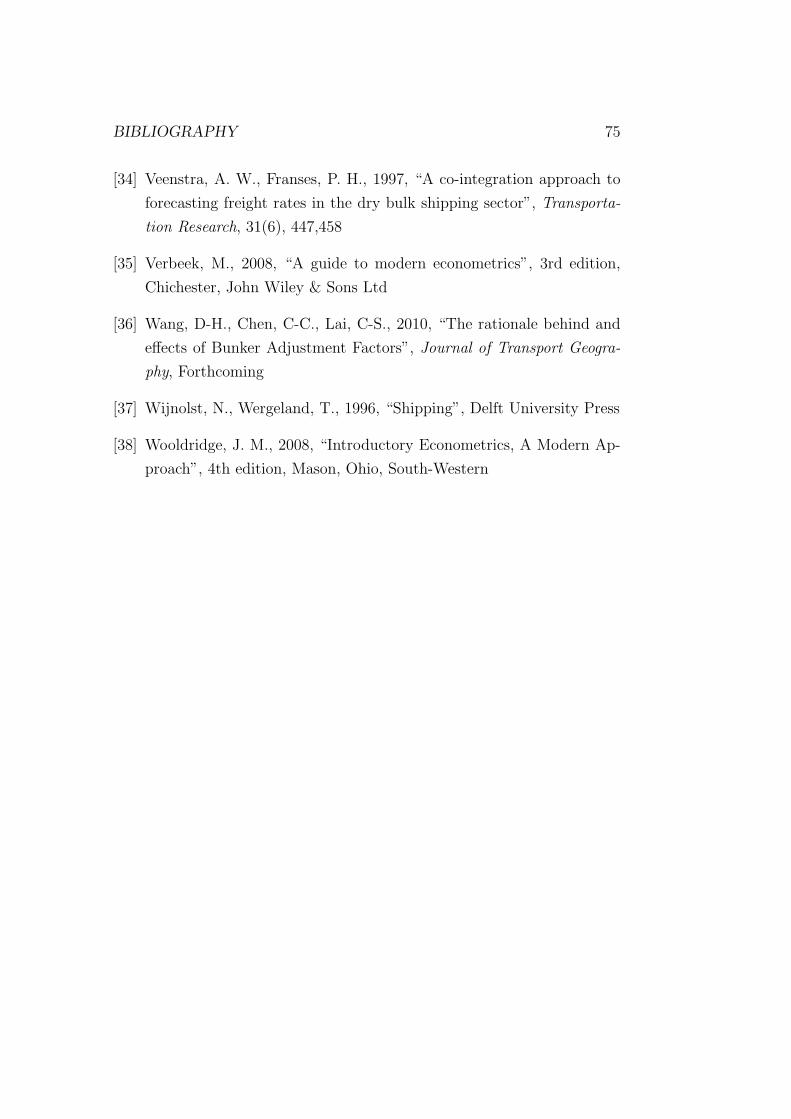
BIBLIOGRAPHY 75
[34] Veenstra, A. W., Franses, P. H., 1997, “A co-integration approach to
forecasting freight rates in the dry bulk shipping sector”, Transporta-
tion Research, 31(6), 447,458
[35] Verbeek, M., 2008, “A guide to modern econometrics”, 3rd edition,
Chichester, John Wiley & Sons Ltd
[36] Wang, D-H., Chen, C-C., Lai, C-S., 2010, “The rationale behind and
effects of Bunker Adjustment Factors”, Journal of Transport Geogra-
phy, Forthcoming
[37] Wijnolst, N., Wergeland, T., 1996, “Shipping”, Delft University Press
[38] Wooldridge, J. M., 2008, “Introductory Econometrics, A Modern Ap-
proach”, 4th edition, Mason, Ohio, South-Western


Appendices
77

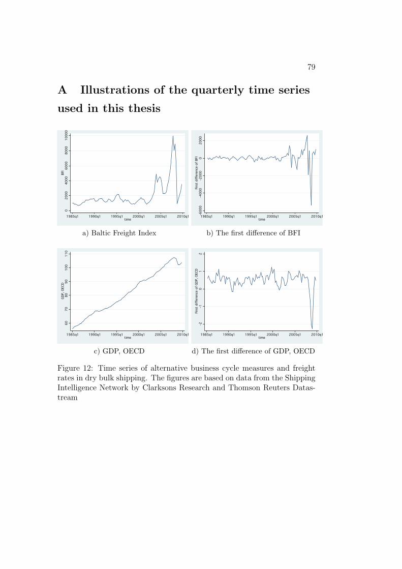
79
A Illustrations of the quarterly time series
used in this thesis
0
0
02000
2000
20004000
4000
40006000
6000
60008000
8000
800010000
1000
010000BFI
BFI
BFI1985q1
1985q1
1985q11990q1
1990q1
1990q11995q1
1995q1
1995q12000q1
2000q1
2000q12005q1
2005q1
2005q12010q1
2010q1
2010q1time
time
time
a) Baltic Freight Index
-6000
-600
0
-6000-4000
-400
0
-4000-2000
-200
0
-20000
0
02000
2000
2000First difference of BFI
Firs
t di
ffer
ence
of B
FI
First difference of BFI1985q1
1985q1
1985q11990q1
1990q1
1990q11995q1
1995q1
1995q12000q1
2000q1
2000q12005q1
2005q1
2005q12010q1
2010q1
2010q1time
time
time
b) The first difference of BFI
60
60
6070
70
7080
80
8090
90
90100
100
100110
110
110GDP, OECD
GDP,
OEC
D
GDP, OECD1985q1
1985q1
1985q11990q1
1990q1
1990q11995q1
1995q1
1995q12000q1
2000q1
2000q12005q1
2005q1
2005q12010q1
2010q1
2010q1time
time
time
c) GDP, OECD
-2
-2
-2-1
-1
-10
0
01
1
12
2
2First difference of GDP, OECD
Firs
t di
ffer
ence
of G
DP, O
ECD
First difference of GDP, OECD1985q1
1985q1
1985q11990q1
1990q1
1990q11995q1
1995q1
1995q12000q1
2000q1
2000q12005q1
2005q1
2005q12010q1
2010q1
2010q1time
time
time
d) The first difference of GDP, OECD
Figure 12: Time series of alternative business cycle measures and freightrates in dry bulk shipping. The figures are based on data from the ShippingIntelligence Network by Clarksons Research and Thomson Reuters Datas-tream
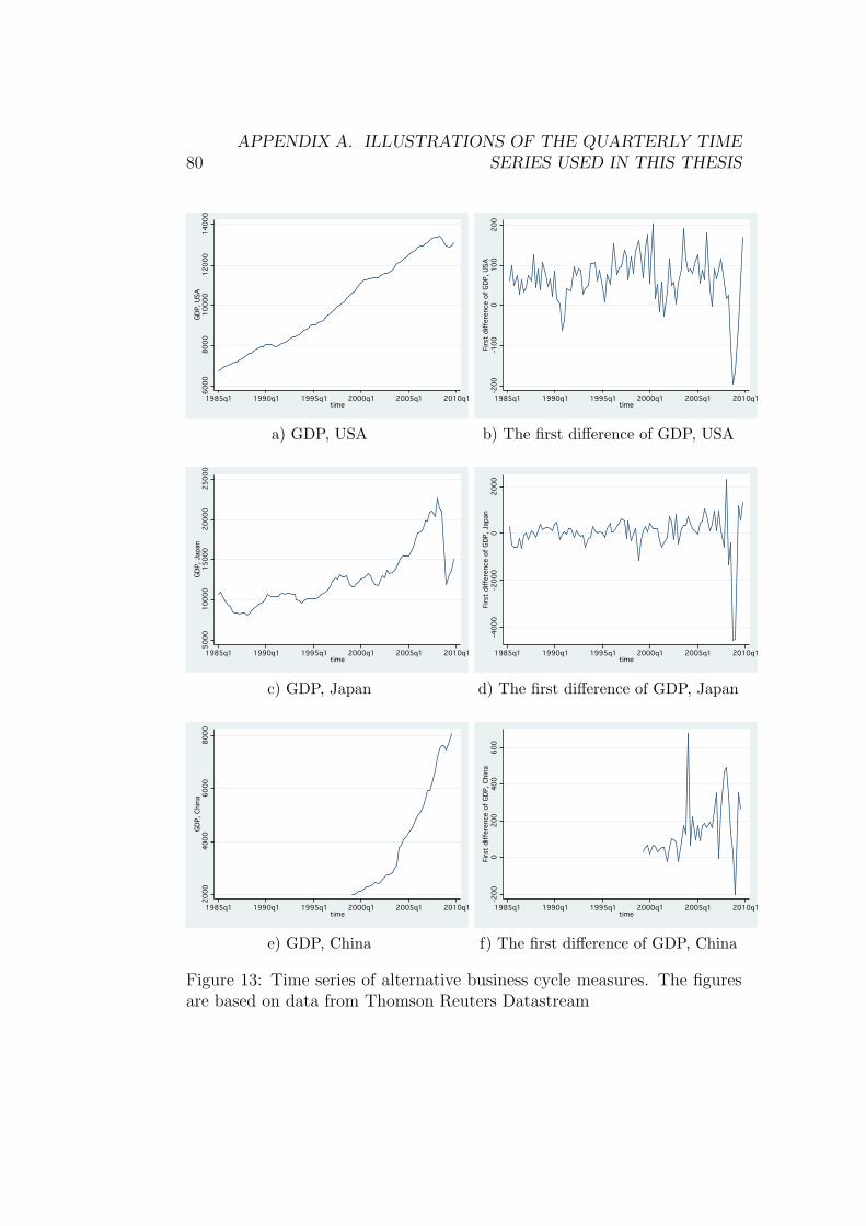
80APPENDIX A. ILLUSTRATIONS OF THE QUARTERLY TIME
SERIES USED IN THIS THESIS
600060
0060008000
8000
80001000010
000
100001200012
000
120001400014
00014000GDP, USA
GDP,
USA
GDP, USA1985q1
1985q1
1985q11990q1
1990q1
1990q11995q1
1995q1
1995q12000q1
2000q1
2000q12005q1
2005q1
2005q12010q1
2010q1
2010q1time
time
time
a) GDP, USA
-200
-200
-200-100
-100
-1000
0
0100
100
100200
200
200First difference of GDP, USA
Firs
t di
ffer
ence
of G
DP, U
SA
First difference of GDP, USA1985q1
1985q1
1985q11990q1
1990q1
1990q11995q1
1995q1
1995q12000q1
2000q1
2000q12005q1
2005q1
2005q12010q1
2010q1
2010q1time
time
time
b) The first difference of GDP, USA
5000
5000
500010000
1000
0
1000015000
1500
0
1500020000
2000
0
2000025000
2500
025000GDP, Japan
GDP,
Jap
an
GDP, Japan1985q1
1985q1
1985q11990q1
1990q1
1990q11995q1
1995q1
1995q12000q1
2000q1
2000q12005q1
2005q1
2005q12010q1
2010q1
2010q1time
time
time
c) GDP, Japan
-4000
-400
0
-4000-2000
-200
0
-20000
0
02000
2000
2000First difference of GDP, Japan
Firs
t di
ffer
ence
of G
DP, J
apan
First difference of GDP, Japan1985q1
1985q1
1985q11990q1
1990q1
1990q11995q1
1995q1
1995q12000q1
2000q1
2000q12005q1
2005q1
2005q12010q1
2010q1
2010q1time
time
time
d) The first difference of GDP, Japan
2000
2000
20004000
4000
40006000
6000
60008000
8000
8000GDP, China
GDP,
Chi
na
GDP, China1985q1
1985q1
1985q11990q1
1990q1
1990q11995q1
1995q1
1995q12000q1
2000q1
2000q12005q1
2005q1
2005q12010q1
2010q1
2010q1time
time
time
e) GDP, China
-200
-200
-2000
0
0200
200
200400
400
400600
600
600First difference of GDP, China
Firs
t di
ffer
ence
of G
DP, C
hina
First difference of GDP, China1985q1
1985q1
1985q11990q1
1990q1
1990q11995q1
1995q1
1995q12000q1
2000q1
2000q12005q1
2005q1
2005q12010q1
2010q1
2010q1time
time
time
f) The first difference of GDP, China
Figure 13: Time series of alternative business cycle measures. The figuresare based on data from Thomson Reuters Datastream
81
B Illustrations of the monthly time series
used in this thesis
0
0
02000
2000
20004000
4000
40006000
6000
60008000
8000
800010000
1000
0
10000BFI monthly
BFI m
onth
ly
BFI monthly1985m1
1985m1
1985m11990m1
1990m1
1990m11995m1
1995m1
1995m12000m1
2000m1
2000m12005m1
2005m1
2005m12010m1
2010m1
2010m1time
time
time
a) Baltic Freight Index
-3000
-300
0
-3000-2000
-200
0
-2000-1000
-100
0
-10000
0
01000
1000
10002000
2000
2000First difference of BFI monthly
Firs
t di
ffer
ence
of B
FI m
onth
ly
First difference of BFI monthly1985m1
1985m1
1985m11990m1
1990m1
1990m11995m1
1995m1
1995m12000m1
2000m1
2000m12005m1
2005m1
2005m12010m1
2010m1
2010m1time
time
time
b) The first difference of BFI
90
90
9095
95
95100
100
100105
105
105110
110
110Ind. prod., OECD
Ind.
pro
d., O
ECD
Ind. prod., OECD1985m1
1985m1
1985m11990m1
1990m1
1990m11995m1
1995m1
1995m12000m1
2000m1
2000m12005m1
2005m1
2005m12010m1
2010m1
2010m1time
time
time
c) Ind., prod., OECD
-2
-2
-2-1
-1
-10
0
01
1
1First difference of Ind. prod., OECD
Firs
t di
ffer
ence
of I
nd. p
rod.
, OEC
D
First difference of Ind. prod., OECD1985m1
1985m1
1985m11990m1
1990m1
1990m11995m1
1995m1
1995m12000m1
2000m1
2000m12005m1
2005m1
2005m12010m1
2010m1
2010m1time
time
time
d) The first difference of Ind., prod.,OECD
Figure 14: Time series of alternative business cycle measures and freightrates in dry bulk shipping. The figures are based on data from the ShippingIntelligence Network by Clarksons Research and Thomson Reuters Datas-tream
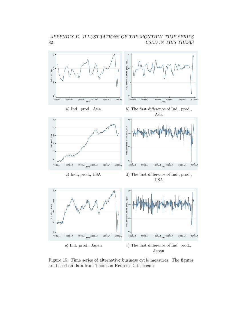
82APPENDIX B. ILLUSTRATIONS OF THE MONTHLY TIME SERIES
USED IN THIS THESIS
9090
909595
9510010
0100105
105
105Ind. prod., AsiaIn
d. p
rod.
, Asia
Ind. prod., Asia1985m1
1985m1
1985m11990m1
1990m1
1990m11995m1
1995m1
1995m12000m1
2000m1
2000m12005m1
2005m1
2005m12010m1
2010m1
2010m1time
time
time
a) Ind., prod., Asia
-2
-2
-2-1
-1
-10
0
01
1
1First difference of Ind. prod., Asia
Firs
t di
ffer
ence
of I
nd. p
rod.
, Asia
First difference of Ind. prod., Asia1985m1
1985m1
1985m11990m1
1990m1
1990m11995m1
1995m1
1995m12000m1
2000m1
2000m12005m1
2005m1
2005m12010m1
2010m1
2010m1time
time
time
b) The first difference of Ind., prod.,Asia60
60
6070
70
7080
80
8090
90
90100
100
100110
110
110Ind. prod., USA
Ind.
pro
d., U
SA
Ind. prod., USA1985m1
1985m1
1985m11990m1
1990m1
1990m11995m1
1995m1
1995m12000m1
2000m1
2000m12005m1
2005m1
2005m12010m1
2010m1
2010m1time
time
time
c) Ind., prod., USA
-4
-4
-4-2
-2
-20
0
02
2
2First difference of Ind. prod., USA
Firs
t di
ffer
ence
of I
nd. p
rod.
, USA
First difference of Ind. prod., USA1985m1
1985m1
1985m11990m1
1990m1
1990m11995m1
1995m1
1995m12000m1
2000m1
2000m12005m1
2005m1
2005m12010m1
2010m1
2010m1time
time
time
d) The first difference of Ind., prod.,USA
70
70
7080
80
8090
90
90100
100
100110
110
110Ind. prod., Japan
Ind.
pro
d., J
apan
Ind. prod., Japan1985m1
1985m1
1985m11990m1
1990m1
1990m11995m1
1995m1
1995m12000m1
2000m1
2000m12005m1
2005m1
2005m12010m1
2010m1
2010m1time
time
time
e) Ind. prod., Japan
-10
-10
-10-5
-5
-50
0
05
5
5First difference of Ind. prod., Japan
Firs
t di
ffer
ence
of I
nd. p
rod.
, Jap
an
First difference of Ind. prod., Japan1985m1
1985m1
1985m11990m1
1990m1
1990m11995m1
1995m1
1995m12000m1
2000m1
2000m12005m1
2005m1
2005m12010m1
2010m1
2010m1time
time
time
f) The first difference of Ind. prod.,Japan
Figure 15: Time series of alternative business cycle measures. The figuresare based on data from Thomson Reuters Datastream
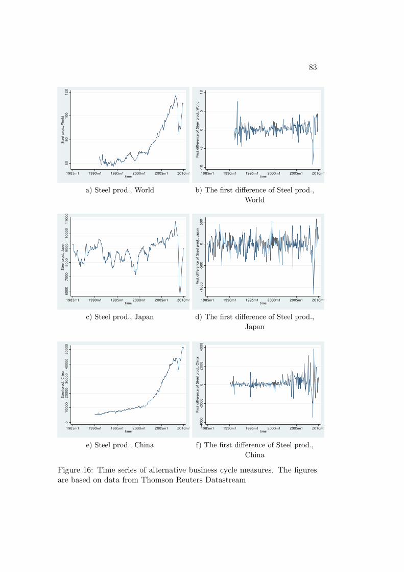
83
60
60
6080
80
80100
100
100120
120
120Steel prod., World
Stee
l pro
d., W
orld
Steel prod., World1985m1
1985m1
1985m11990m1
1990m1
1990m11995m1
1995m1
1995m12000m1
2000m1
2000m12005m1
2005m1
2005m12010m1
2010m1
2010m1time
time
time
a) Steel prod., World
-10
-10
-10-5
-5
-50
0
05
5
510
10
10First difference of Steel prod., World
Firs
t di
ffer
ence
of S
teel
pro
d., W
orld
First difference of Steel prod., World1985m1
1985m1
1985m11990m1
1990m1
1990m11995m1
1995m1
1995m12000m1
2000m1
2000m12005m1
2005m1
2005m12010m1
2010m1
2010m1time
time
time
b) The first difference of Steel prod.,World
6000
6000
60007000
7000
70008000
8000
80009000
9000
900010000
1000
0
1000011000
1100
011000Steel prod., Japan
Stee
l pro
d., J
apan
Steel prod., Japan1985m1
1985m1
1985m11990m1
1990m1
1990m11995m1
1995m1
1995m12000m1
2000m1
2000m12005m1
2005m1
2005m12010m1
2010m1
2010m1time
time
time
c) Steel prod., Japan
-1000
-100
0
-1000-500
-500
-5000
0
0500
500
500First difference of Steel prod., Japan
Firs
t di
ffer
ence
of S
teel
pro
d., J
apan
First difference of Steel prod., Japan1985m1
1985m1
1985m11990m1
1990m1
1990m11995m1
1995m1
1995m12000m1
2000m1
2000m12005m1
2005m1
2005m12010m1
2010m1
2010m1time
time
time
d) The first difference of Steel prod.,Japan
0
0
010000
1000
0
1000020000
2000
0
2000030000
3000
0
3000040000
4000
0
4000050000
5000
0
50000Steel prod., China
Stee
l pro
d., C
hina
Steel prod., China1985m1
1985m1
1985m11990m1
1990m1
1990m11995m1
1995m1
1995m12000m1
2000m1
2000m12005m1
2005m1
2005m12010m1
2010m1
2010m1time
time
time
e) Steel prod., China
-4000
-400
0
-4000-2000
-200
0
-20000
0
02000
2000
20004000
4000
4000First difference of Steel prod., China
Firs
t di
ffer
ence
of S
teel
pro
d., C
hina
First difference of Steel prod., China1985m1
1985m1
1985m11990m1
1990m1
1990m11995m1
1995m1
1995m12000m1
2000m1
2000m12005m1
2005m1
2005m12010m1
2010m1
2010m1time
time
time
f) The first difference of Steel prod.,China
Figure 16: Time series of alternative business cycle measures. The figuresare based on data from Thomson Reuters Datastream

84APPENDIX B. ILLUSTRATIONS OF THE MONTHLY TIME SERIES
USED IN THIS THESIS200
200
200400
400
400600
600
600800
800
800Steel prod., AustraliaSt
eel p
rod.
, Aus
tral
iaSteel prod., Australia1985m1
1985m1
1985m11990m1
1990m1
1990m11995m1
1995m1
1995m12000m1
2000m1
2000m12005m1
2005m1
2005m12010m1
2010m1
2010m1time
time
time
a) Steel prod., Australia
-200
-200
-200-100
-100
-1000
0
0100
100
100200
200
200First difference of Steel prod., Australia
Firs
t di
ffer
ence
of S
teel
pro
d., A
ustr
alia
First difference of Steel prod., Australia1985m1
1985m1
1985m11990m1
1990m1
1990m11995m1
1995m1
1995m12000m1
2000m1
2000m12005m1
2005m1
2005m12010m1
2010m1
2010m1time
time
time
b) The first difference of Steel prod.,Australia
0
0
020
20
2040
40
4060
60
6080
80
80Iron ore imp, E-Asia
Iron
ore
imp,
E-A
sia
Iron ore imp, E-Asia1985m1
1985m1
1985m11990m1
1990m1
1990m11995m1
1995m1
1995m12000m1
2000m1
2000m12005m1
2005m1
2005m12010m1
2010m1
2010m1time
time
time
c) Iron ore imp., E-Asia
-10
-10
-10-5
-5
-50
0
05
5
510
10
1015
15
15First difference of Iron ore imp., E-Asia
Firs
t di
ffer
ence
of I
ron
ore
imp.
, E-A
sia
First difference of Iron ore imp., E-Asia1985m1
1985m1
1985m11990m1
1990m1
1990m11995m1
1995m1
1995m12000m1
2000m1
2000m12005m1
2005m1
2005m12010m1
2010m1
2010m1time
time
time
d) The first difference of Iron oreimp., E-Asia
0
0
0200
200
200400
400
400600
600
600800
800
8001000
1000
1000Exports, OECD
Expo
rts,
OEC
D
Exports, OECD1985m1
1985m1
1985m11990m1
1990m1
1990m11995m1
1995m1
1995m12000m1
2000m1
2000m12005m1
2005m1
2005m12010m1
2010m1
2010m1time
time
time
e) Exports, OECD
-100
-100
-100-50
-50
-500
0
050
50
50First difference of Exports, OECD
Firs
t di
ffer
ence
of E
xpor
ts, O
ECD
First difference of Exports, OECD1985m1
1985m1
1985m11990m1
1990m1
1990m11995m1
1995m1
1995m12000m1
2000m1
2000m12005m1
2005m1
2005m12010m1
2010m1
2010m1time
time
time
f) The first difference of Exports,OECD
Figure 17: Time series of alternative business cycle measures. The figuresare based on data from the Shipping Intelligence Network by ClarksonsResearch and Thomson Reuters Datastream

85
3000
3000
30004000
4000
40005000
5000
50006000
6000
60007000
7000
70008000
8000
8000Exports, Japan
Expo
rts,
Jap
an
Exports, Japan1985m1
1985m1
1985m11990m1
1990m1
1990m11995m1
1995m1
1995m12000m1
2000m1
2000m12005m1
2005m1
2005m12010m1
2010m1
2010m1time
time
time
a) Exports, Japan
-2000
-200
0
-2000-1000
-100
0
-10000
0
01000
1000
10002000
2000
2000First difference of Exports, Japan
Firs
t di
ffer
ence
of E
xpor
ts, J
apan
First difference of Exports, Japan1985m1
1985m1
1985m11990m1
1990m1
1990m11995m1
1995m1
1995m12000m1
2000m1
2000m12005m1
2005m1
2005m12010m1
2010m1
2010m1time
time
time
b) The first difference of Exports,Japan
0
0
02000
2000
20004000
4000
40006000
6000
60008000
8000
8000Imports, Japan
Impo
rts,
Jap
an
Imports, Japan1985m1
1985m1
1985m11990m1
1990m1
1990m11995m1
1995m1
1995m12000m1
2000m1
2000m12005m1
2005m1
2005m12010m1
2010m1
2010m1time
time
time
c) Imports, Japan
-1000
-100
0
-1000-500
-500
-5000
0
0500
500
500First difference of Imports, Japan
Firs
t di
ffer
ence
of I
mpo
rts,
Jap
an
First difference of Imports, Japan1985m1
1985m1
1985m11990m1
1990m1
1990m11995m1
1995m1
1995m12000m1
2000m1
2000m12005m1
2005m1
2005m12010m1
2010m1
2010m1time
time
time
d) The first difference of Imports,Japan
20
20
2025
25
2530
30
3035
35
3540
40
40Coal exp., total
Coal
exp
., to
tal
Coal exp., total1985m1
1985m1
1985m11990m1
1990m1
1990m11995m1
1995m1
1995m12000m1
2000m1
2000m12005m1
2005m1
2005m12010m1
2010m1
2010m1time
time
time
e) Coal exports, total
-5
-5
-50
0
05
5
510
10
10First difference of Coal exp., total
Firs
t di
ffer
ence
of C
oal e
xp.,
tota
l
First difference of Coal exp., total1985m1
1985m1
1985m11990m1
1990m1
1990m11995m1
1995m1
1995m12000m1
2000m1
2000m12005m1
2005m1
2005m12010m1
2010m1
2010m1time
time
time
f) The first difference of Coal exports,total
Figure 18: Time series of alternative business cycle measures. The figuresare based on data from Thomson Reuters Datastream
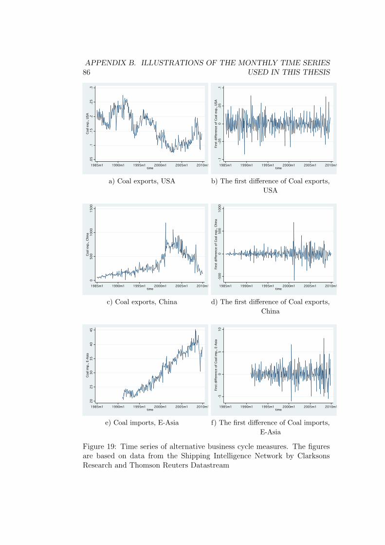
86APPENDIX B. ILLUSTRATIONS OF THE MONTHLY TIME SERIES
USED IN THIS THESIS.05
.05
.05.1
.1
.1.15
.15
.15.2
.2
.2.25
.25
.25.3
.3
.3Coal exp., USACo
al e
xp.,
USA
Coal exp., USA1985m1
1985m1
1985m11990m1
1990m1
1990m11995m1
1995m1
1995m12000m1
2000m1
2000m12005m1
2005m1
2005m12010m1
2010m1
2010m1time
time
time
a) Coal exports, USA
-.1
-.1
-.1-.05
-.05
-.050
0
0.05
.05
.05.1
.1
.1First difference of Coal exp., USA
Firs
t di
ffer
ence
of C
oal e
xp.,
USA
First difference of Coal exp., USA1985m1
1985m1
1985m11990m1
1990m1
1990m11995m1
1995m1
1995m12000m1
2000m1
2000m12005m1
2005m1
2005m12010m1
2010m1
2010m1time
time
time
b) The first difference of Coal exports,USA
0
0
0500
500
5001000
1000
10001500
1500
1500Coal exp., China
Coal
exp
., Ch
ina
Coal exp., China1985m1
1985m1
1985m11990m1
1990m1
1990m11995m1
1995m1
1995m12000m1
2000m1
2000m12005m1
2005m1
2005m12010m1
2010m1
2010m1time
time
time
c) Coal exports, China
-500
-500
-5000
0
0500
500
5001000
1000
1000First difference of Coal exp., China
Firs
t di
ffer
ence
of C
oal e
xp.,
Chin
a
First difference of Coal exp., China1985m1
1985m1
1985m11990m1
1990m1
1990m11995m1
1995m1
1995m12000m1
2000m1
2000m12005m1
2005m1
2005m12010m1
2010m1
2010m1time
time
time
d) The first difference of Coal exports,China
20
20
2025
25
2530
30
3035
35
3540
40
4045
45
45Coal imp., E-Asia
Coal
imp.
, E-A
sia
Coal imp., E-Asia1985m1
1985m1
1985m11990m1
1990m1
1990m11995m1
1995m1
1995m12000m1
2000m1
2000m12005m1
2005m1
2005m12010m1
2010m1
2010m1time
time
time
e) Coal imports, E-Asia
-5
-5
-50
0
05
5
510
10
10First difference of Coal imp., E-Asia
Firs
t di
ffer
ence
of C
oal i
mp.
, E-A
sia
First difference of Coal imp., E-Asia1985m1
1985m1
1985m11990m1
1990m1
1990m11995m1
1995m1
1995m12000m1
2000m1
2000m12005m1
2005m1
2005m12010m1
2010m1
2010m1time
time
time
f) The first difference of Coal imports,E-Asia
Figure 19: Time series of alternative business cycle measures. The figuresare based on data from the Shipping Intelligence Network by ClarksonsResearch and Thomson Reuters Datastream
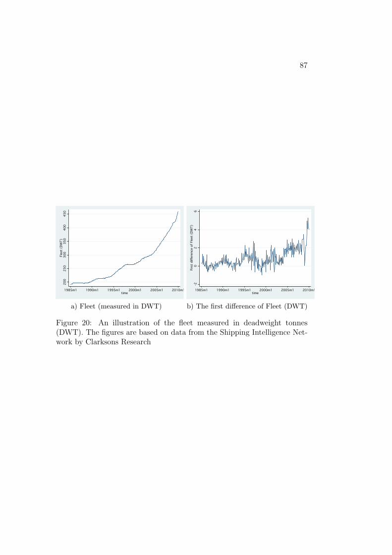
87
200
200
200250
250
250300
300
300350
350
350400
400
400450
450
450Fleet (DWT)
Flee
t (D
WT)
Fleet (DWT)1985m1
1985m1
1985m11990m1
1990m1
1990m11995m1
1995m1
1995m12000m1
2000m1
2000m12005m1
2005m1
2005m12010m1
2010m1
2010m1time
time
time
a) Fleet (measured in DWT)
-2
-2
-20
0
02
2
24
4
46
6
6First difference of Fleet (DWT)
Firs
t di
ffer
ence
of F
leet
(DW
T)
First difference of Fleet (DWT)1985m1
1985m1
1985m11990m1
1990m1
1990m11995m1
1995m1
1995m12000m1
2000m1
2000m12005m1
2005m1
2005m12010m1
2010m1
2010m1time
time
time
b) The first difference of Fleet (DWT)
Figure 20: An illustration of the fleet measured in deadweight tonnes(DWT). The figures are based on data from the Shipping Intelligence Net-work by Clarksons Research

88 APPENDIX C. STATA COMMANDS
C Stata commands
This appendix offers a presentation of the Stata commands that are most
frequently used in this thesis. In order to make it more reader-friendly,
commands that are not considered to be of particular importance have
been omitted from the appendix. Let the BFI be defined as variable Y ,
while the various business cycle measures are represented by the variable
X.
Declare data to be time-series data
generate time = m(1985m1) + n −1
format time %tm
tsset time
Transform the data into logarithmic form
gen lnY = log(Y )
gen lnX = log(X)
Calculate the first difference of the variables
gen dlnY = lnY − l.lnY
gen dlnX = lnX − l.lnX
Dickey Fuller-test for stationarity of the time series and their first
differences (The Stata command depends on the model specification.
Lags(#) tells Stata how many lags to include in order to adjust for
autocorrelation.)
No drift or trend: dfuller variable, regress nocons lags(#)
Drift, but no trend: dfuller variable, regress lags(#)

89
Drift and trend: dfuller variable, regress lags(#) trend
Cointegration-test
reg lnY lnX
predict r lnY lnX, resid
dfuller r lnY lnX, noconst regress
Error Correction Model
reg dlnY l.r lnY lnX dlnX