dsge model restrictions for structural var identification · dsge model restrictions for structural...

DSGE Model Restrictions for Structural VARIdentification∗

Philip Liua and Konstantinos Theodoridisb

aInternational Monetary FundbBank of England

The identification of reduced-form VAR models has beenthe subject of numerous debates in the literature. Differentsets of identifying assumptions can lead to very different con-clusions regarding the effects of shocks. This paper proposesa theoretically consistent identification strategy using restric-tions implied by a DSGE model. Monte Carlo simulations sug-gest that both quantitative and qualitative restrictions workwell together, where they act as complements to each other,in minimizing errors in finding the correct VAR identification.When using misspecified model restrictions, the data tend topush the identified VAR responses away from the misspecifiedmodel and closer to the true data-generating process.

JEL Codes: F31, E52.

1. Introduction

Since the pioneer work of Sims (1980), vector autoregressive (VAR)models have been used extensively by applied researchers, fore-casters, and policymakers to address a range of economic issues.Although VAR models have been very successful in capturing thedynamic properties of the macroeconomic time-series data, the

∗Copyright c© 2012 Bank of England. The views expressed in this workare those of the authors and do not necessarily reflect those of the Bankof England and the International Monetary Fund. The authors would like tothank Richard Harrison, Matthias Paustian, the editors Frank Smets and JohnWilliams, an anonymous referee, and participants at the ESAM2009 meetingfor helpful comments and insightful discussions. Correspondences: Bank of Eng-land, Monetary Analysis, Bank of England, Threadneedle Street, London EC2R8AH, United Kingdom. E-mail addresses: [email protected],[email protected].

61

62 International Journal of Central Banking December 2012

decomposition of these statistical relationships back to coherent eco-nomic stories is still under large debate. The key source of thisdisagreement arises from the difficulty in identifying structural dis-turbances from a set of reduced-form residuals. The sampling infor-mation in the data is not sufficient, and several assumptions areneeded in order to recover the mapping between the structural andthe reduced-form errors.1 However, the outcome of the VAR analysisdepends crucially on these assumptions, and the various competingidentification restrictions cannot be easily tested against the data.

The literature has proposed a number of different exact-identification strategies. First, and most popular, is the Choleskishort-run restriction on the VAR’s reduced-form covariance matrix.Under the Choleski scheme, the ordering of the variables is partic-ularly important for the structural economic interpretation of theVAR (see Lutkepohl 1993 and Hamilton 1994). Furthermore, asCanova (2005) explains, the Choleski decomposition implies “zero-type” restrictions that are rarely consistent with dynamic stochasticgeneral equilibrium (DSGE) models. A similar procedure was intro-duced by Blanchard and Quah (1989) by imposing long-run relation-ships that are consistent with economic theory. However, a number ofstudies such as Chari, Kehoe, and McGrattan (2005), Erceg, Guerri-eri, and Gust (2005), Christiano, Eichenbaum, and Vigfusson (2006),and Ravenna (2007) have concluded that long-run restrictions areinadequate in recovering the true structural disturbances. The mainreason is that it is often difficult to obtain an accurate estimateof the long-run impacts because of the truncation bias associatedwith VAR models. Therefore, imposing long-run restrictions basedon these bias estimates can lead to misleading conclusions.

More recently, Faust (1998), Canova and De Nicolo (2002), andUhlig (2005) propose an identification scheme that imposes “sign” or“qualitative” restrictions on the structural responses. The strategyrecognizes there are an infinite number of observationally equivalentmappings between the structural and the reduced-form errors, andthe idea of the sign restriction is to select a subset of these mappingsthat are consistent with certain qualitative features. An attractivefeature of this procedure is that it makes VAR and DSGE models

1The discussions here focus on exact VAR identification.

Vol. 8 No. 4 DSGE Model Restrictions 63

more comparable than other identification strategies. Researcherscan then use qualitative information in the form of sign restrictionsimplied by DSGE models to help identify structural VAR shocks;for example, Peersman and Straub (2009) and Liu (2010) use thisapproach. Although attractive to applied researchers, as highlightedby Uhlig (2005) and explicitly illustrated by Fry and Pagan (2011),this type of identification scheme fails to deliver a unique identifica-tion mapping. There can be a range of impulse responses that areconsistent with the sign restrictions. This leads to large uncertaintyaround the model’s estimates (see Paustian 2007) and makes policyinference less informative.

Uhlig (2005) also discusses an alternative procedure known as the“penalty-function” approach. The idea is to find the set of orthog-onal shocks that minimize a specific penalty function. This is cer-tainly a less agnostic approach relative to the pure sign-restrictionmethod. Nevertheless, the procedure produces a unique set of struc-tural shocks and therefore reduces the degree of uncertainty relatedto the identification procedure. However, the choice of the penaltyfunction remains arbitrary and difficult to motivate from an eco-nomic perspective.

An alternative procedure was proposed by Del Negro andSchorfheide (2004), who developed a methodology to generate aprior distribution using a DSGE model for a time-series VAR. TheDSGE-VAR approach relaxes the tight theoretical restrictions of theDSGE model by making use of the model and data, summarized bythe likelihood of the model. While the DSGE-VAR has been a veryuseful tool for model comparison and forecasting, as Sims (2008)pointed out, it remains difficult to use the DSGE-VAR for policyanalysis—for example, impulse response analysis. The main reasonis that the DSGE-VAR still faces the same identification problemsas standard VAR models. Del Negro and Schorfheide (2004) suggestusing the identification matrix from the DSGE model as an approx-imation; however, the resultant variance-covariance matrix will nolonger be the same as the estimated DSGE-VAR (see Del Negro andSchorfheide 2004, footnote 17).

This paper proposes an identification strategy that extendsUhlig’s (2005) penalty-function approach to a more formal setting.In particular, we construct a penalty function that is based onquantitative and qualitative restrictions implied by a DSGE model.


To assess the usefulness of the proposed identification strategy, wepresent a series of Monte Carlo experiments. First, we investigatewhether the proposed algorithm can recover the true set of structuralshocks given the correct set of restrictions; second, we assess how theproposed identification strategy performs using quantitative restric-tions from a misspecified model; third, we investigate using only apartial set of qualitative restrictions. Lastly, we present an applica-tion using a seven-variable VAR model estimated on U.S. data.

A number of interesting results emerge from the analysis. First,the proposed identification strategy systematically gives a smallerbias compared with other identification schemes such as the Choleskidecomposition and pure sign restrictions. Second, despite usingrestrictions implied by a misspecified model, the data (summarized bythe reduced-form covariance matrix) tend to push the VAR responsesaway from the misspecified model and closer to the true data-generating process (DGP). Third, when we only impose a partialset of qualitative sign restrictions, the proposed method consistentlyyields a smaller bias relative to the pure sign-restriction approach.Our results suggest that both quantitative and qualitative restrictionswork well together, where they act as complements to each other, inminimizing errors in finding the correct VAR identification.

The paper is organized as follows. Section 2 discusses the advan-tages of the proposed methodology. Section 3 outlines the methodol-ogy of the proposed identification strategy. Section 4 briefly describesthe Monte Carlo experiments and outlines the medium-scale DSGEmodel used for the data-generating process. Section 5 reports theresults from the Monte Carlo experiments. Section 6 presents anapplication of the proposed identification strategy using a seven-variable VAR model estimated on U.S. data. Section 7 containsconcluding remarks and proposes direction for future research.

2. The Usefulness of the Proposed Methodology

Our starting point is the work of Pagan (2003), who argues that thereis an inherent trade-off between theoretical and empirical coherencefor macroeconomic models.2 DSGE models are perhaps the most

2Pagan (2003) illustrates this by placing various types of models along a con-cave “modeling frontier” with the degree of theoretical coherence and the degreeof empirical coherence along each axis.


transparent example of this negative trade-off between theoreticalconsistency and data coherence. These models often place a largeamount of restrictions based on simplified economic theory, whichcould limit its ability to fit the data well. The literature has pro-gressed significantly along this dimension following the pioneeredwork of Smets and Wouters (2007)—who illustrated that DSGEmodels can be designed to fit the data well, at the same time keep-ing its attractive theoretical coherence structure. However, the issueof model misspecification still remains (see discussions in Del Negroand Schorfheide 2009).

Our proposed approach offers an additional angle to this debateby creating a structural VAR model that mimics the DSGE model aslong as the restrictions implied by the latter regarding the mappingbetween the reduced-form and structural errors do not significantlyviolate the estimated variance-covariance matrix of the VAR residu-als. One can think of the approach presented here as bringing the sta-tistical VAR analysis closer to the structural DSGE models along the“Pagan curve” but without sacrificing empirical coherence. Despiteapplying more restrictions on the behavior of the impulse responsefunctions of the VAR, the proposed method does not change eitherthe empirical fit or the forecasting performance—see proposition 1of Waggoner and Zha (1999)—of the VAR model. Rather, it simplyselects a unique identification mapping from the infinite number ofobservationally equivalent ones. This is a subtle but important dif-ference from Del Negro and Schorfheide’s (2004) DSGE-VAR, wherethe approach here maintains the same variance-covariance matrix asthe reduced-form representation of the VAR for structural identifi-cation. Our identified VAR can also be a useful cross-check againstthe structural model to evaluate the simplified assumptions of themodel.

3. Methodology

3.1 A Review of the Identification Problem

The use of VAR models to address key macroeconomic policy ques-tions depends crucially on the identification of the reduced-formresiduals. Even though several procedures have been proposed inthe literature, shock identification remains a highly controversial


issue. To illustrate the identification problem, consider the followingstylized structural model:3

A0Yt = A(L)hYt + ηt (1)

Yt = A−10 A(L)hYt + A−1

0 ηt, (2)

where Yt is an (n×1) vector of endogenous variables, A0 is an (n×n )matrix of coefficients, A(L)h = A1L+ · · ·+AhLh is an hth-order lagpolynomial, and E(ηtη

′t) = I gives the variance-covariance matrix of

the structural innovations. Equation (1) is the structural model andequation (2) is the corresponding reduced-form representation. Thekey parameters of interest are A0 and A(L). However, the samplinginformation in the data is not sufficient to identify both A0 and A(L)separately without employing further identifying restrictions. Thereare infinite combinations of A0 and A(L) that all imply exactly thesame probability distribution for the observed data. To see this, pre-multiply the model in (1) by a full rank matrix Q, which leads tothe following new model:

QA0Yt = QA(L)Yt + Qηt (3)

Yt = A−10 Q−1QA(L)Yt + A−1

0 Q−1Qηt. (4)

The reduced-form representation of the two models in equa-tions (2) and (4) are exactly the same. That implies both modelsin (1) and (3) are observationally equivalent. Without additionalassumptions—identifying restrictions—no conclusions regarding thestructural behavior of the “true” model can be drawn from the data.

As explained by Canova (2005, chapter 4), popular identificationschemes such as the Choleski decomposition and long-run restric-tions impose “zero-type” restrictions that cannot be easily justi-fied by a large class of DSGE models. In particular, DSGE modelshardly display the type of recursive structures that are typicallyassumed by Choleski or long-run identification schemes. This raisesthe question of whether these identification schemes are the appro-priate choices in relation to the economic theory. Furthermore, fromthe work Carlstrom, Fuerst, and Paustian (2009), it is known that

3For the moment, we remain agnostic as to the form of the structural modelor where it comes from. More details are provided in the next sub-section.


these restrictions can severely distort the impulse response functionif they are not consistent with the true DGP.

The identification scheme proposed by Faust (1998), Canova andDe Nicolo (2002), and Uhlig (2005) seem to overcome some of thesedifficulties by imposing sign and/or shape (pure sign) restrictions onthe structural responses. Although attractive to applied researchers,the procedure fails to deliver a unique identification mapping as itis highlighted by Uhlig (2005) and Fry and Pagan (2011). In otherwords, there can be a range of impulse responses that are consistentwith the sign restrictions. This can lead to large uncertainty aroundthe model’s estimates and less reliable inference.

3.2 The Mapping between the DSGE and the VAR Model

To see the links between the structural and the reduced-form VARmodel, it is useful to explore the mapping between the two. To bemore specific, we are going to consider the class of structural modelsthat are usually based on agents’ optimization behavior and ration-al expectation formation (DSGE models). Generally, the solutionof a linearized DSGE model can be summarized by the followingstate-space representation:4

Xt = B (θ) Xt−1 + Γ (θ) ηt (5)

Yt = A (θ) Xt, (6)

where Xt is an n×1 vector of state variables, Yt is an m×1 vector ofvariables observed by an econometrician, and ηt represents an k × 1vector of economic shocks such that E(ηt) = 0 and E(ηtη

′t) = I.5

The matrices A(θ), B(θ), and Γ(θ) are functions of the underlyingstructural parameters of the DSGE model. Equation (6) is usuallyreferred to as the state equation (or policy function) that describesthe evolution of the underlying economy, and equation (5) is theobservation equation that relates the state of the economy with theset of observable variables. For notational convenience, we will drop

4The solution of the model can be obtained by using either Blanchard andKahn (1980) or Sims’s (2002) type algorithms.

5In the notation here, xt also includes the current values of exogenous shockprocesses.


the indication that the matrices A, B, and Γ are functions of thestructural parameters θ.

From the work of Christiano, Eichenbaum, and Vigfusson (2006),Fernandez-Villaverde et al. (2007), and Ravenna (2007), the state-space representation of the DSGE model described above has aninfinite-order VAR process representation, VAR(∞), if and only ifthe eigenvalues of the following matrix,

M =[In − Γ (AΓ)−1

A]B, (7)

are less than one in absolute terms and the number of the shockscoincides with the number of observed variables, i.e., m = k. Thisis known as the “poor man’s invertibility condition” or simply the“invertibility condition” as in Fernandez-Villaverde et al. (2007). Ifthis condition holds, the set of observable variables Yt can be writtenas a VAR(∞) such that

Yt =∞∑

j=1

ΔjYt−j + AΓηt, (8)

where

Δj = ABM j−1Γ (AΓ)−1.

On the other hand, a reduced-form VAR(h) model can be esti-mated on a set of stationary macroeconomic time series Yt to providea summary of its statistical properties,

yt =h∑

j=1

Ajyt−j + vt, (9)

where vt is normally distributed with zero mean and variance-covariance matrix Σv . Assuming the DSGE model in equation (9)is the true data-generating process (DGP) for Yt, the reduced-formVAR in equation (9) can provide a reasonably good approximationof the process Yt as the number of lags (h) tends to infinity. In sucha case, the mapping between the reduced-form and structural shocks


can be uniquely defined as (Christiano, Eichenbaum, and Vigfusson2006, proposition 1)

vt = AΓηt (10)

or

Σv ≡ E (vtv ′t) = AΓΓ′A′. (11)

It is this unique mapping that this paper exploits to help identifyreduced-form VAR shocks.

3.3 DSGE Restrictions for Structural VARs

In addition to the pure sign-restriction approach, Uhlig (2005) alsodiscusses an alternative procedure known as the “penalty function.”The idea behind the procedure is to find a set of orthogonal shocksthat minimizes a specific penalty function. However, the choice ofthe penalty function remains arbitrary and difficult to motivate froman economic perspective. The identification strategy described hereessentially extends the penalty-function approach to a more formalsetting. In particular, we exploit the mapping between the DSGEand the VAR model as shown earlier to construct the penalty func-tion. This is attractive because it provides a theoretically consis-tent way of identifying structural VAR shocks, and the identifyingassumptions are motivated from restrictions implied by DSGE mod-els. Furthermore, the procedure can help bring together the twodistinct approaches of macroeconomic modeling.

Assuming the DSGE model is the true DGP with variance-covariance matrix AΓΓ′A′, Lutkepohl and Poskitt (1991) show thatthe estimated variance-covariance of a VAR(h) model converges tothe true variance-covariance when the number of lags tends to infin-ity (h → ∞) as the sample size tends to infinity (T → ∞). The rateat which the sample size tends to infinity must be faster than therate at which h3 tends to infinity, that is,

Σv → AΓΓ′A′ ash3

T→ 0, (12)

where Σv is the estimated VAR variance-covariance or the reduced-form covariance. In practice, the two key assumptions underlying


the above condition undoubtedly break down. First, mostly DSGEmodels are tools designed to explain certain subsets of stylized facts.Despite the recent success in improving its empirical performance,misspecification remains a concern (Del Negro et al. 2007). Second,samples of macroeconomic time-series data are limited, so the num-ber of lags that can be included in the VAR is quite restrictive.Consequently, the estimated VAR variance-covariance can be quitedifferent from the one implied by the DSGE model.

In the pure sign-restriction case, Σv is decomposed into Σv =CP (ω)P (ω)′C ′, where C is the Choleski factor of Σv , P (ω) is anorthonormal matrix such that P (ω)P (ω)′ = I, and ω denotes avector of rotation angles—each element of this vector lies between0 and π. The matrix P (ω) is selected in such a way to meet theresearcher’s belief regarding the qualitative properties of the impulseresponses. As discussed earlier, the selection of P (ω) is non-unique.The proposed identification strategy here essentially selects a uniquematrix P (ω) to minimize the “distance” between the contemporane-ous response of the VAR and the one implied by the DSGE model.The procedure can be summarized as the following minimizationproblem:

ω∗ = arg minω

⎧⎨⎩

∥∥∥vec(CP (ω) − AΓ

)∥∥∥2

+k∑

j=1

m∑i=1

δijI (signij)

⎫⎬⎭(13)

subject to

P (ω) P (ω)′ − I = 0, (14)

where ‖ · ‖2 stands for the Euclidian norm, I(signij) is an indicatorfunction for variable i in response to shock j that takes values 0 if thesign restrictions are satisfied and 1 otherwise, and δij is a positivenumber. A few remarks are worth noting. The first part of equa-tion (13) resembles Uhlig’s (2005) penalty function, although herethe function is based on restrictions from a DSGE model. The sec-ond part of equation (13) is analogous to the pure sign restrictions.The parameter δij controls for a set of sign restrictions we want to


impose on the model.6 The key difference is that by imposing addi-tional restrictions from a DSGE model, it will ensure a unique iden-tification matrix CP (ω∗) for the VAR. The difference between theidentified VAR responses relative to the DSGE model will depend onhow plausible the theoretical restrictions are in the face of the datasummarized by A(L)h and Σv . If these restrictions are deemed faraway from the empirical evidence, then the difference can be quitelarge, and vice versa. There is no closed-form solution readily avail-able for the above minimization problem, so we resort to numericalmethods for the simulation experiments. However, Judd (1998, the-orem 4.7.1) shows that under some regularity conditions, the vectorω∗ is unique, implying that P (ω∗) is also unique.

4. Monte Carlo Experiments

This section sets out a series of Monte Carlo experiments designedto evaluate the usefulness of the proposed identification procedure.

4.1 The Model for the Data-Generating Process

The model used for the Monte Carlo study is based on the workby Smets and Wouters (2007).7 This is an estimated medium-scaleDSGE model that incorporates various sources of nominal andreal frictions to match U.S. post-war business-cycle fluctuations. Inthis model, the steady state of the economy follows a determinis-tic trend according to the rate of labor-augmenting technologicalprogress. Households select consumption and labor effort to max-imize their non-separable utility preferences. Agents’ consumptionbehavior exhibits habit formation, and households are assumed tosupply differentiated labor services to firms. This gives households

6The first part of equation (13) penalizes positive and negative deviationsfrom the DSGE responses in exactly the same manner. However, it is of greatereconomic interest for the VAR to deliver the same signs for the impulse responsescompared with finding the smallest absolute deviation. The algorithm achievesthis by attaching some positive weight to δij . Note that the optimization algo-rithm is not sensitive to the value of δij , and in our implementation we setδij = 1.

7Smets and Wouters’ (2007) model is based on the earlier work of Smets andWouters (2003) and Christiano, Eichenbaum, and Evans (2005).


monopoly power over wage negotiations, and therefore aggregatewages are sticky. In addition, households, who face capital adjust-ment costs, optimally decide how much capital to rent to firms andhow much capital to accumulate.

On the production side, firms minimize the cost of productionby optimally selecting the amount of labor and capital inputs sub-ject to capital utilization costs and the wage rate set by house-holds. Given demands for their product, firms reoptimize pricesinfrequently in a Calvo-type fashion. Finally, wages and prices thatare not reoptimized every period are partially indexed to the pastinflation. The appendix summarizes the key linearized equation ofthe model. Readers who are interested in the agents’ decision prob-lems are advised to consult the references mentioned above directly.The model’s key parameters’ values are taken directly from Smetsand Wouters’ (2007) study and summarized in table 7.

In the original model, Smets and Wouters assume seven exoge-nous driving processes or shocks. These are required in order tomatch the seven observable variables used in the estimation. Here,we simplify the model to contain only four shocks, namely a govern-ment spending shock, a price markup shock, a wage markup shock,and a monetary policy shock.8

4.2 The Monte Carlo Design

To investigate the properties of the identification strategy describedin section 3.3, we set up two Monte Carlo experiments. In the firstpart of the experiments, we test the proposed identification strategyusing the true model specification as well as restrictions implied bythe following series of misspecified models:

• M0: Benchmark• M1: Model with no habit formation (h = 0)• M2: Model with no price and wage indexation (ip = iw = 0)• M3: Model with no moving-average terms for price and wage

markup shocks (μp = μw = 0)

8The original model also includes a net worth shock, a technology shock, andan investment-specific shock. In principle, it is possible to include all seven shocksfor the Monte Carlo experiments, but this would increase the computation burdenfor the Monte Carlo experiment significantly.


• M4: Model with no habit formation, price and wage indexation(M1 and M2)

• M5: Model with no interest rate smoothing term in the Taylorrule (ρ = 0)

We compare the results using the proposed identification withthe other identification strategies, such as Choleski ordering and thepure sign-restriction approach. Note that if we place no weight onthe first part of the objective function (quantitative restrictions),our procedure collapses to the pure sign-restriction scheme, but thiswill not yield a unique P (ω) as discussed earlier. Next, we perform asimilar set of experiments but using only a subset of sign restrictionsimplied by the model:

• Case I: No Government Spending Restrictions, δi,1 = 0 fori = 1, . . . , 4

• Case II: No Interest Rate Restrictions, δi,2 = 0 for i = 1, . . . , 4• Case III: No Wage Markup Restrictions, δi,3 = 0 for i =

1, . . . , 4• Case IV: No Price Markup Restrictions, δi,4 = 0 for i =

1, . . . , 4• Case V: No Interest Rate and Wage Markup Restrictions,

δi,2 = δi,3 = 0∀i• Case VI: No Interest Rate and Government Spending Restric-

tions, δi,1 = δi,2 = 0∀i• Case VII: Only Government Spending Restrictions, δi,j = 0

for i = 1, . . . , 4 and j = 2, . . . , 4• Case VIII: Only Interest Rate Restrictions, δi,j = 0 for

i = 1, . . . , 4 and j = 1, 2 and 4• Case IX: Only Price Markup Restrictions, δi,j = 0 for i =

1, . . . , 4 and j = 1, . . . , 3

This allows us to investigate the role played by the pure sign-restrictions component of our proposed objective function (qualita-tive restrictions),

∑kj=1

∑mi=1 δijI(signij). In general, the simulation

experiment follows these few steps:

(i) Simulate data—Yt—of 200 observations of the observablevector (output growth, inflation, wage growth, and the


nominal interest rate) using the model and parametersdescribed in section 4.1.9

(ii) Estimate a DSGE model (M0, . . . , M5) using maximum-likelihood estimation (MLE). The likelihood of the modelis constructed via the Kalman filter and maximized usingSim’s CSMINWEL algorithm. This gives the contempora-neous impact matrix of the DSGE model (A(θi)Γ(θi)) asfunctions of the model’s structural parameters (θi)—wherei = M0,. . . ,M5.

(iii) Estimate a reduced-form VAR(2) model using ordinaryleast squares (OLS) and compute the variance-covariancematrix (Σv ) of the reduced-form errors.

(iv) Decompose Σv into CP (ωi)P (ωi)′C ′ and find an orthonor-mal matrix P (ω∗

i ) such that it minimizes the loss functionin equation (13). We use Matlab’s fminunc function to findthe minimum. To ensure that the minimization algorithmfinds the unique global minimum, we repeat the minimiza-tion procedure 1,000 times using different random startingvalues.

(v) Construct impulse responses from the identified structuralVAR (SVAR) using CP (ω∗

i ).(vi) Repeat the above steps 500 times.

5. Results from the Monte Carlo Study

5.1 Bias of the SVAR Impulse Response Functions

To assess the performance of our proposed methodology, we computethe bias of the impulse responses from the true DGP as

biasT = 100T∑

t=1

M∑i=1

K∑j=1

|Ψt,i,j − Ψt,i,j |Ψt,i,j

, (15)

where Ψt,i,j is the t’th period’s impulse response of the estimatedbenchmark or VAR model for variable i to shock j, Ψt,i,j is the DGP

9We simulate 10,000 observations and we keep only the 200.


equivalent, and the bias is calculated as the sum across all the Mvariables and K shocks up to periods T . Before turning to the dis-cussion of the results, it is useful to identify where the SVAR biasmay be coming from by reexpressing the SVAR in the form similarto equation (1):

A(L)Yt = et = A−10 ηt (16)

Yt = A(L)−1A−10 ηt = R(L)A−1

0 ηt. (17)

From equation (17), one can see that the response of Yt to the under-lying structural innovation, ηt, is influenced both by the reduced-form moving-average terms, R(L), and by the identifying restrictionsplaced on A0. Erceg, Guerrieri, and Gust (2005) usefully categorizethis bias into three components:

SVAR bias = R-bias + A-bias + Truncation bias. (18)

The first part, the “R-bias,” reflects the small-sample error in esti-mating the reduced-form moving-average terms, the R(L) coeffi-cients in equation (17). The second part, referred to as the “A-bias,”reflects the error associated with transforming the reduced forminto its structural form by imposing certain identifying restrictions,the A0 matrix. Lastly, the “truncation bias” arises because a finite-ordered VAR (h < ∞) is chosen to approximate the true dynamicsimplied by the model, a VARMA process. Kapetanios, Pagan, andScott (2007) document that the truncation bias from medium- tolarge-scale models can be very large. However, it is important to rec-ognize that the three types of biases are not necessary independentof each other; they can interact and exacerbate the overall bias ofthe SVAR responses. For example, using a fixed sample size, a largertruncation bias can increase the R-bias related to the estimation ofthe reduced-form coefficients. Similarly, for a fixed set of identify-ing assumptions, the imprecision in estimating R(L) can exacer-bate the A-bias associated with the identification of the structuralshocks.

In contrast to Erceg, Guerrieri, and Gust (2005), we find thatthe truncation bias plays a dominant role in explaining the differ-ence between the VAR and the DSGE model’s responses at longer


Figure 1. Truncation Bias (Accumulated) of theVAR Model

1020

3040

5

5

10

15

200

50

100

150

200

250

300

350

400

VAR LagsIRF Periods

Bia

s

horizons. To illustrate this, figure 1 plots the truncation bias of anSVAR model along different lag lengths.10 As one might expect, for afixed number of lags, the bias is larger at longer horizons (see expla-nations in Ravenna 2007). On the other hand, the bias is a monotonicfunction decreasing with the number of lags included in the VAR. Itis interesting to note that the bias decreases in a non-linear fashion.This is in line with the evidence provided by Kapetanios, Pagan, andScott (2007) that in order to approximate a medium- to large-scaleDSGE model, one would require a significantly large number of lagsfor the VAR.

The speed in which the truncation bias decreases with the num-ber of lags will depend on the model’s specification and parameters.More specifically, Fernandez-Villaverde et al. (2007) point out that

10The SVAR model is estimated based on a simulated data sample of 100,000and the identification matrix is computed using the benchmark model restrictions(M0).


the closer the largest (absolute value) eigenvalue of the matrix M inequation (7) is to one, the more lags are needed in order to approxi-mate the true DGP. In our case, the largest eigenvalue of the matrixM is indeed very close to one and therefore it is not surprising thata large-order VAR is needed to approximate the dynamics of themodel.11 For discussions of the empirical results in the next sub-sections, we will focus on shorter horizons, where the truncationbias is less important.

5.2 SVAR Identification Using the Correct Model Restrictions

Table 1 reports the bias from our first set of simulation experiments.Columns 1, 4, 7, and 10 report the bias for all of the DSGE modelsdescribed in section 4.2 at the one-, two-, eight-, and twelve-quarterhorizon. Similarly, columns 2, 5, 8, and 11 present the same meas-ures for the identified SVAR models. Finally, columns 3, 6, 9, and12 display the ratio of these quantities.

Looking at the benchmark model (M0) along the first row oftable 1, we can see that the proposed SVAR closely matches the biasfrom the estimated DSGE at short horizons. In longer horizons, thetruncation bias from the estimated VAR dominates and the DSGEmodel outperforms. This result is not that surprising given what wehad discussed in the previous section, but nevertheless it is usefulto know that our proposed algorithm is capable of recovering thetrue impulse responses if the correct set of model restrictions wereapplied.

To compare the proposed identification with other identifica-tion strategies, figure 2 plots the responses of the Choleski VARmodel (solid-circle line), VAR model with sign restrictions (solid-cross line) implied by the model, the estimated DSGE model (solidline), and the true response (dashed line) against our proposedSVAR (dotted-dashed line).12 In all cases, the Choleski and sign-restriction identification schemes produced impulse responses that

11We also experimented with a simple three-equation New Keynesian modelwhere the eigenvalue of the matrix M is much smaller, in which case a VAR(2)together with the proposed identification strategy provides an excellent matchwith the DGP’s impulse responses. These results are available on request.

12For the Choleski decomposition, the variables are ordered as output, inflation,wage growth, and short-term interest rate.


Tab

le1.

Acc

um

ula

ted

Bia

sfo

rM

issp

ecifi

edM

odel

san

dth

eSVA

RM

odel

Per

iod

1Per

iods

2Per

iods

8Per

iods

12

DSG

ESVA

RR

atio

DSG

ESVA

RR

atio

DSG

ESVA

RR

atio

DSG

ESVA

RR

atio

M0

1.5

1.6

0.9

2.5

3.7

0.7

39.2

98.4

0.4

68.4

190.

20.

4M

16.

15.

91.

010

.39.

51.

161

.913

1.8

0.5

85.3

230.

00.

4M

22.

11.

91.

16.

34.

41.

474

.110

9.7

0.7

97.2

213.

40.

5M

34.

25.

00.

89.

87.

91.

272

.211

7.4

0.6

109.

820

3.3

0.5

M4

5.7

5.4

1.0

11.3

9.3

1.2

68.7

128.

90.

510

4.1

235.

30.

4M

512

.812

.91.

019

.819

.61.

011

7.5

190.

00.

616

4.0

263.

40.

6

Note

s:T

he

accu

mula

ted

bia

sis

calc

ula

ted

asth

esu

m(a

cros

sdiff

eren

tnu

mber

ofper

iods)

ofth

eab

solu

teper

cent

age

diff

eren

cebet

wee

nth

ees

tim

ated

DSG

Em

odel

orth

eVA

R’s

impuls

ere

spon

ses

wit

hth

eD

GP.T

he

rati

om

easu

reis

sim

ply

the

bia

sof

the

esti

mat

edD

SG

Em

odel

rela

tive

toth

atof

the

SVA

Rm

odel

.


Figure 2. Median Impulse Response Functions of theBenchmark Model: 500 Samples of 200 Observations

0 5 10 15 20

−1.2

−1

−0.8

−0.6

−0.4

−0.2

0

Output

Wag

e−M

arku

p

0 5 10 15 200

0.1

0.2

0.3

0.4

0.5

Interest Rate

Wag

e−M

arku

p

0 5 10 15 200

0.1

0.2

0.3

0.4

Inflation

Wag

e−M

arku

p

0 5 10 15 20

0

0.2

0.4

0.6

0.8

1Wages

Wag

e−M

arku

p

EstimatedDGPVARCholSign

0 5 10 15 20−0.6

−0.5

−0.4

−0.3

−0.2

−0.1

0

0.1

Output

Pric

e−M

arku

p

0 5 10 15 20

0

0.1

0.2

0.3

0.4

0.5

Interest Rate

Pric

e−M

arku

p

0 5 10 15 20

0

0.2

0.4

0.6

0.8

1Inflation

Pric

e−M

arku

p

0 5 10 15 20

−1.5

−1

−0.5

0

Wages

Pric

e−M

arku

p


0 5 10 15 20

−0.5

0

0.5

1Output

Gov

ernm

ent

0 5 10 15 20

0

0.2

0.4

0.6

0.8

Interest Rate

Gov

ernm

ent

0 5 10 15 20

0

0.1

0.2

0.3

0.4

Inflation

Gov

ernm

ent

0 5 10 15 20−0.2

0

0.2

0.4

0.6Wages

Gov

ernm

ent


0 5 10 15 20

−1

−0.8

−0.6

−0.4

−0.2

0

0.2

Output

Mon

etar

y

0 5 10 15 20

0

0.2

0.4

0.6

0.8

1Interest Rate

Mon

etar

y

0 5 10 15 20−0.6

−0.4

−0.2

0

0.2

Inflation

Mon

etar

y

0 5 10 15 20

−0.6

−0.5

−0.4

−0.3

−0.2

−0.1

0

Wages

Mon

etar

y


are much further away from the DGP. The standard “price puzzle,”for example, is evident in the Choleski scheme, and different recur-sive ordering structures produced very similar results. It is interest-ing to note that even though the sign restrictions deliver the rightsigns by construction, they consistently overestimate the impact ofthe shock.

The summary statistics in table 2, which shows the ratio of thebias relative to the proposed SVAR, reveal a similar conclusion. Thesize of the bias using the Choleski scheme is between eight and eleventimes larger than the proposed identification strategy at shorterhorizons, and the sign restriction scheme is thirty-one to forty-eighttimes larger. At longer horizons, the truncation bias dominates andthe differences are much smaller.


Table 2. SVAR Bias Relative to Other IdentificationMethodologies

Horizon SVARC

SVARD

SVARS

SVARD

1 11.0 48.52 8.3 31.93 3.0 10.24 3.0 10.28 2.8 5.512 2.2 3.316 1.9 2.720 1.8 2.4

Note: SVARD, SVARC , and SVARS correspond to the SVAR(2) model bias thatarises using DSGE, Choleski, and sign restrictions, respectively.

5.3 Proposed Methodology Using Misspecified ModelRestrictions

One natural question to ask is how the proposed identificationscheme performs if the wrong set of quantitative restrictions wereimposed, given that model misspecification was one of our initialmotivations for the proposed identification strategy. Rows 2–6 intable 1 report the bias for the estimated misspecified DSGE modelsand the SVAR.13 This is certainly not an exhaustive list of poten-tial misspecifications one can consider, but it does provide a way ofevaluating the usefulness of the proposed identification scheme whenrestrictions are derived from misspecified models.

The model with no interest rate smoothing term in the Taylorrule (M5) gives the largest bias relative to the true DGP. Since theVAR identification also depends on the restrictions implied by themisspecified model, the bias for the SVAR model is also the largestfor M5. At shorter horizons (one and two quarters), where the com-parison is more informative, the bias of the SVAR models is smallerthan that of the misspecified models.14

13The quantitative restrictions of the SVAR were also based on the samemisspecified model.

14The exception is model M5, where the bias between the misspecified modeland the VAR is very similar.


This is an interesting result: even though the identification bias(A-bias) is larger because we are using restrictions from a misspec-ified model, the data (summarized by the reduce-form VAR covari-ance matrix) tends to push the SVAR responses closer to the trueDGP. Therefore, information from the data is useful in correctingsome of the bias arising from using misspecified model restrictions.The results from this experiment show that despite imposing incor-rect quantitative restrictions from a misspecified DSGE model, theproposed methodology is still useful in identifying the true underly-ing structural shocks.

5.4 Proposed Methodology Using Partial Sign Restrictions

Paustian (2007) demonstrates that if we identify all the shocks usingsign restrictions, then the resulting rotation would be closer to thatimplied by the DGP. However, it is common for an applied econo-mist to identify only a small subset of structural shocks derived froma VAR system—say, a supply, demand, and policy shock—or thatthe researcher only have strong priors on a subset of restrictions.In this sub-section, we look at the bias generated by the proposedprocedure using only a partial set of sign restrictions. This allows usto investigate whether the proposed identification is sensitive to theset of assumed qualitative restrictions.

Tables 3–5 report the ratio of the bias of the proposed identifi-cation relative to the pure sign-restriction approach across the ninedifferent cases and six DSGE models outlined earlier. A ratio lessthan one indicates that our proposed method yields a smaller biascompared with the pure sign-restriction approach. The results sug-gest that the improvement in using the proposed methodology canbe substantial. In the case where we have the correct quantitativerestrictions (M0), the average improvement is more than 90 percent.More realistically, we would be working with a misspecified model.Looking at the results using the five misspecified models, M1 to M5,we still achieve significant improvements in all cases up to the four-quarter horizon. There is only one case (case V) where we see a smalldeterioration at the eight- and twelve-quarter horizon. On average,the proposed method improves the bias over the pure sign-restrictionscheme by about 50 percent. In general, we find that by imposingmore and more sign restrictions, this reduces the bias of the SVAR


Table 3. Results of Cases I, II, and III

Case I Case II Case III

Q1 Q4 Q8 Q12 Q1 Q4 Q8 Q12 Q1 Q4 Q8 Q12

M0 0.02 0.06 0.05 0.06 0.01 0.09 0.12 0.12 0.01 0.06 0.05 0.06M1 0.19 0.34 0.27 0.40 0.34 0.74 0.93 0.96 0.57 0.61 0.64 0.67M2 0.08 0.27 0.24 0.37 0.32 0.72 0.91 0.95 0.54 0.59 0.62 0.66M3 0.12 0.32 0.27 0.39 0.33 0.73 0.93 0.97 0.56 0.60 0.65 0.69M4 0.17 0.32 0.26 0.40 0.33 0.71 0.89 0.95 0.58 0.60 0.62 0.67M5 0.69 0.80 0.72 0.73 0.56 0.65 0.81 0.96 0.39 0.67 0.79 0.79

Note: Each table entry displays the accumulated bias of the DSGE-identified VARmodel relative to the pure sign-restrictions SVAR accumulated bias.

Table 4. Results of Cases IV, V, and VI

Case IV Case V Case VI

Q1 Q4 Q8 Q12 Q1 Q4 Q8 Q12 Q1 Q4 Q8 Q12

M0 0.01 0.06 0.07 0.08 0.01 0.08 0.10 0.11 0.01 0.08 0.06 0.07M1 0.35 0.44 0.32 0.37 0.43 0.76 1.23 1.19 0.30 0.42 0.64 0.73M2 0.32 0.40 0.30 0.36 0.43 0.71 1.11 1.10 0.22 0.29 0.53 0.65M3 0.34 0.43 0.29 0.34 0.44 0.72 1.15 1.12 0.28 0.34 0.56 0.67M4 0.34 0.42 0.30 0.35 0.46 0.77 1.21 1.19 0.31 0.42 0.66 0.76M5 0.46 0.61 0.57 0.58 0.57 0.98 1.44 1.29 0.54 0.52 0.57 0.62


with respect to the DGP—a result that is consistent with Paustian(2007) finding.15

Overall, our results suggest that both quantitative and quali-tative restrictions work well together, where they act as comple-ments to each other, in minimizing errors in finding the correct VARidentification.

15We perform a series of Monte Carlo experiments by imposing zero, one, two,three, and four sets of sign restrictions. The results are available upon request.


Table 5. Results of Cases VII, VIII, and IX

Case VII Case VIII Case IX

Q1 Q4 Q8 Q12 Q1 Q4 Q8 Q12 Q1 Q4 Q8 Q12

M0 0.01 0.07 0.08 0.09 0.02 0.06 0.06 0.07 0.01 0.07 0.07 0.07M1 0.41 0.60 0.85 0.94 0.61 0.59 0.64 0.74 0.23 0.35 0.62 0.72M2 0.41 0.58 0.82 0.91 0.55 0.61 0.63 0.71 0.22 0.35 0.66 0.78M3 0.44 0.62 0.88 0.96 0.56 0.63 0.68 0.76 0.24 0.36 0.64 0.75M4 0.42 0.56 0.77 0.88 0.60 0.58 0.64 0.73 0.22 0.37 0.66 0.76M5 0.61 0.80 0.91 0.95 0.72 0.77 0.85 0.88 0.33 0.34 0.42 0.50


6. Application: Seven-Variable SVAR Model for theUnited States

To illustrate how the proposed identification scheme can be appliedin practice, we estimate a seven-variable VAR using U.S. data from1966:Q1 to 2004:Q4. The data set is taken from the Smets andWouters (2007) paper which includes the log-difference of real GDP,real consumption, real investment and the real wage, log hoursworked, the log-difference of the GDP deflator, and the federal fundsrate. Although Smets and Wouters (2007) compare the estimatedDSGE model’s forecast performance with reduced-form VARs, theydid not present any comparisons between the DSGE model’s impulseresponse functions with a VAR model. This partly reflects the diffi-culty in finding the appropriate set of identifying restrictions for theVAR. From that perspective, our identification scheme is a naturalcandidate for comparison analysis. One can view this as a diagnos-tic tool for analyzing the dynamic behavior of the estimated DSGEmodel.

We follow the same procedure set out earlier in section 3.3,and the restrictions are based on Smets and Wouters’ (2007) orig-inal model with all seven shocks.16 First, we estimate the VAR

16The seven shocks include a government spending shock, a price markupshock, a wage markup shock, a monetary policy shock, a net worth shock, atechnology shock, and an investment-specific shock.


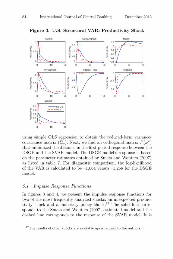
Figure 3. U.S. Structural VAR: Productivity Shock

0 10 200

0.5

1Output

Pro

duct

ivity

0 10 200

0.1

0.2

0.3

Consumption

Pro

duct

ivity

0 10 20−0.8−0.6−0.4−0.2

00.2

Hours

Pro

duct

ivity

0 10 20

0

0.5

1

Investment

Pro

duct

ivity

0 10 20

−0.2

−0.1

0Interest Rate

Pro

duct

ivity

0 10 20

−0.2

−0.1

0Inflation

Pro

duct

ivity

0 10 20

0

0.1

0.2

0.3

0.4

Wages

Pro

duct

ivity

DSGEVAR

using simple OLS regression to obtain the reduced-form variance-covariance matrix (Σv ). Next, we find an orthogonal matrix P (ω∗)that minimized the distance in the first-period response between theDSGE and the SVAR model. The DSGE model’s response is basedon the parameter estimates obtained by Smets and Wouters (2007)as listed in table 7. For diagnostic comparison, the log-likelihoodof the VAR is calculated to be –1,064 versus –1,256 for the DSGEmodel.

6.1 Impulse Response Functions

In figures 3 and 4, we present the impulse response functions fortwo of the most frequently analyzed shocks: an unexpected produc-tivity shock and a monetary policy shock.17 The solid line corre-sponds to the Smets and Wouters (2007) estimated model and thedashed line corresponds to the response of the SVAR model. It is

17The results of other shocks are available upon request to the authors.


Figure 4. U.S. Structural VAR: Monetary Policy Shock

0 10 20

−1

−0.5

0

Output

Mon

etar

y

0 10 20−1

−0.5

0

Consumption

Mon

etar

y0 10 20

−1

−0.5

0Hours

Mon

etar

y

0 10 20

−1.5

−1

−0.5

0

Investment

Mon

etar

y

0 10 200

0.5

1Interest Rate

Mon

etar

y

0 10 20−1

−0.5

0

Inflation

Mon

etar

y

0 10 20−0.4

−0.3

−0.2

−0.1

0

Wages

Mon

etar

y

DSGEVAR

worth highlighting that all the variables’ responses have the samesign across the two models. However, there are some interesting dif-ferences in terms of the magnitudes and adjustment paths to theshocks.

For the productivity shock, the SVAR model tends to suggest asmaller impact on hours worked and the nominal interest rate. Theimpact on consumption, real wages, and inflation is slightly higherbut less persistent. For the monetary policy shock, the SVAR modelgives a larger but more temporary response for inflation. On theother hand, the SVAR displays a much more persistent behavior forhours worked, real wages, and the interest rate compared with theDSGE model. Interestingly, the response of output, consumption,and investment are very similar across the two models.

6.2 Forecast-Error-Variance Decomposition

In addition to the impulse response analysis, we also compute theforecast-error-variance (FEV) decomposition for both models—seetable 6. For the SVAR, productivity and investment shocks are the


Tab

le6.

For

ecas

t-V

aria

nce

Dec

ompos

itio

n

Pri

ceW

age

Pro

duct

ivity

Pre

fere

nce

Gov

ernm

ent

Inve

stm

ent

Mon

etar

yM

arkup

Mar

kup

Outp

ut

VA

RD

SG

EVA

RD

SG

EVA

RD

SG

EVA

RD

SG

EVA

RD

SG

EVA

RD

SG

EVA

RD

SG

E

Q1

35.4

13.5

4.8

26.0

3.4

38.9

46.6

13.8

0.0

5.3

2.4

2.4

7.4

0.1

Q4

32.2

13.7

7.6

23.3

4.6

33.7

45.8

15.3

1.0

5.9

2.9

4.7

6.0

3.5

Q8

29.9

13.2

7.8

22.8

4.7

32.2

42.4

15.3

2.1

6.0

5.8

4.7

7.3

5.7

Q12

29.6

13.0

7.8

22.4

4.7

31.6

41.8

15.9

2.4

6.3

6.2

4.9

7.4

5.9

∞27

.44.

818

.00.

10.

046

.828

.814

.89.

50.

314

.41.

81.

831

.4

Con

sum

pti

onQ

18.

61.

621

.982

.25.

00.

663

.31.

00.

611

.70.

01.

20.

41.

7Q

48.

43.

720

.569

.64.

61.

260

.20.

91.

012

.12.

64.

52.

78.

0Q

88.

33.

720

.165

.94.

61.

359

.11.

01.

112

.03.

24.

53.

711

.5Q

128.

33.

720

.164

.84.

61.

359

.01.

21.

112

.53.

34.

73.

711

.8∞

21.9

12.0

19.3

0.2

1.2

2.1

14.8

4.9

2.7

0.5

25.9

1.2

14.3

79.0

Hou

rsQ

159

.519

.70.

723

.630

.336

.97.

412

.80.

34.

60.

50.

71.

31.

8Q

470

.07.

71.

015

.221

.123

.85.

326

.80.

210

.00.

45.

82.

110

.7Q

865

.44.

13.

38.

314

.515

.96.

123

.81.

28.

66.

210

.83.

328

.5Q

1256

.83.

35.

05.

810

.812

.34.

817

.83.

16.

413

.011

.56.

642

.9∞

42.7

0.1

9.2

0.4

4.0

20.2

3.0

0.1

7.7

0.7

25.4

2.3

7.9

76.2

(con

tinu

ed)

Vol. 8 No. 4 DSGE Model Restrictions 87Tab

le6.

(Con

tinued

)

Pri

ceW

age

Pro

duct

ivity

Pre

fere

nce

Gov

ernm

ent

Inve

stm

ent

Mon

etar

yM

arkup

Mar

kup

Inve

stm

ent

VA

RD

SG

EVA

RD

SG

EVA

RD

SG

EVA

RD

SG

EVA

RD

SG

EVA

RD

SG

EVA

RD

SG

E

Q1

0.8

3.4

0.4

3.1

1.1

1.0

97.7

88.1

0.0

2.1

0.1

1.7

0.0

0.6

Q4

6.5

5.5

2.3

2.3

1.2

1.6

71.0

83.3

1.6

1.9

6.6

3.1

10.8

2.3

Q8

6.4

5.6

2.2

2.3

2.5

1.8

57.3

81.9

2.8

2.0

12.5

3.1

16.4

3.4

Q12

7.0

5.4

2.1

2.2

2.7

1.7

56.1

82.3

2.9

2.0

12.7

3.1

16.3

3.4

∞0.

321

.63.

20.

01.

616

.522

.020

.711

.60.

242

.22.

419

.238

.4

Inte

rest

Rat

esQ

122

.49.

617

.520

.61.

71.

929

.61.

714

.154

.714

.88.

00.

03.

4Q

419

.714

.718

.615

.40.

73.

421

.312

.516

.728

.821

.912

.91.

212

.3Q

819

.813

.617

.711

.20.

73.

516

.322

.216

.719

.326

.311

.12.

619

.2Q

1221

.812

.516

.810

.00.

93.

414

.124

.815

.917

.427

.29.

93.

321

.9∞

32.6

13.3

12.3

2.8

2.1

13.9

4.9

6.0

11.4

1.5

29.6

3.3

7.2

59.2

Inflat

ion

Q1

0.0

3.7

1.6

0.5

1.0

0.3

27.3

1.9

1.4

2.1

29.3

72.8

39.3

18.7

Q4

2.1

5.2

0.9

0.9

0.6

0.6

27.3

4.2

0.7

4.7

26.4

48.2

42.0

36.3

Q8

4.3

4.8

0.9

1.0

0.7

0.7

25.6

5.4

0.9

5.8

26.3

39.0

41.3

43.3

Q12

7.0

4.5

1.4

1.0

0.9

0.8

23.8

5.6

1.3

6.1

26.3

36.8

39.3

45.2

∞30

.94.

16.

20.

51.

84.

40.

01.

16.

33.

934

.85.

419

.980

.6

Wag

esQ

112

.91.

73.

31.

215

.00.

17.

70.

30.

40.

76.

331

.154

.564

.9Q

415

.03.

16.

21.

313

.70.

211

.71.

41.

21.

75.

931

.346

.361

.1Q

816

.33.

66.

31.

313

.50.

211

.81.

51.

31.

76.

030

.944

.860

.8Q

1217

.43.

56.

41.

413

.20.

211

.61.

61.

51.

86.

430

.543

.561

.0∞

36.8

13.4

11.7

0.1

1.7

10.1

3.9

11.2

9.6

0.7

34.9

3.2

1.2

61.3


main drivers of the FEV for output growth, whereas in the DSGEmodel, preference and government spending shocks play the domi-nant role. Similarly for consumption growth, investment shocks aremore important than preference shocks in the SVAR model. Forhours worked, productivity shocks explain over 50 percent of theFEV as opposed to the wage markup shock identified in the DSGEmodel. Investment shocks are the key factor in explaining investmentgrowth across both models.

These observations highlight an important contrast across thetwo models: the SVAR tends to suggest that real shocks, such asinvestment and productivity shocks, play a relatively more impor-tant role than nominal shocks (government spending and wagemarkup shocks) for real economic variables. The sum of real shocksaccounts for 80 percent of output, 87 percent of consumption, 70percent of hours worked, and 65 percent of investment at the twelve-quarter horizon.18 On the other hand, the DSGE model tends tosuggest that both real and nominal shocks play an equally importantrole.

For the nominal interest rate, both models suggest that the con-tribution to the FEV is (roughly) equally divided among all sevenshocks over the medium term. The DSGE model identifies bothprice and wage markup shocks to be the key drivers of the FEVfor inflation, whereas the SVAR also attributes part of the FEVto investment shocks. For wage growth, while both models agreeon the importance of wage markup shocks, the SVAR points to amuch smaller role for price markup shocks over the medium term.Another interesting feature is that the DSGE model identifies wagemarkup shocks to be the dominant contributor of the unconditionalvariance for interest rate, inflation, and wage growth, whereas theSVAR highlights the importance of productivity and price markupshocks.

7. Conclusion

Issues relating to the identification of VAR models have been sub-ject to numerous debates in the literature. The key source of

18We classify real shocks to include productivity, preference, and investmentshocks. All other shocks are classified as nominal shocks.


this disagreement arises from finding a set of appropriate identi-fying assumptions to disentangle the reduced-form residuals backinto structural disturbances. The sampling information in the datais often insufficient to distinguish between these different sets ofassumptions. This paper proposes an identification strategy thatextends Uhlig’s (2005) penalty-function approach to a more formalsetting. In particular, we construct a penalty function that is basedon both quantitative and qualitative restrictions implied by a DSGEmodel. We present a series of Monte Carlo experiments to assess theusefulness of the proposed identification strategy. We also presentan application using a seven-variable VAR model estimated on U.S.data and compare this with the results obtained from a medium-scaleDSGE model by Smets and Wouters (2007).

By using the correct model restrictions, our proposed algorithmis successful in recovering the true structural identification matrixfrom the reduced-form VAR. In contrast to Erceg, Guerrieri, andGust (2005), we find that the truncation bias is the dominant sourceof the bias in the estimated impulse response functions—particularlyat longer horizons. Our result is consistent with the findings inKapetanios, Pagan, and Scott (2007).

A number of interesting results emerge from the Monte Carloanalysis. First, the proposed identification strategy systematicallygives a smaller bias compared with other identification schemes suchas the Choleski decomposition and pure sign restrictions. Second,despite using restrictions implied by a misspecified model, the data(summarized by the reduced-form covariance matrix) tend to pushthe VAR responses away from the misspecified model and closerto the true DGP. Third, when we only impose a partial set ofsign restrictions, the proposed method consistently yields a smallerbias relative to the pure sign-restriction approach. Our results sug-gest that both quantitative and qualitative restrictions work welltogether, where they act as complements to each other, in minimiz-ing errors in finding the correct VAR identification.

The identification procedure proposed here is mainly appliedto VAR models with a relatively small number of variables. Butincreasingly, the empirical literature emphasizes the importance ofestimating statistical models based on a large information set. Exam-ples include the large Bayesian VAR model put forward by Band-bura, Giannone, and Reichlin (2010) and the factor-augmented VAR


model of Bernanke, Boivin, and Eliasz (2005). Future research couldtherefore be directed towards exploiting information contained inDSGE models to help identify VAR models with a large number ofvariables.

Appendix. The Model

This appendix briefly discusses some of the key linearized equilib-rium conditions of Smets and Wouters’ (2007) model. Readers whoare interested in the agents’ decision problems are advised to con-sult the references mentioned above directly. All the variables areexpressed as log-deviations from their steady-state values, Et denotesexpectation formed at time t, “−” denotes the steady-state values,and all the shocks (ηi

t) are assumed to be normally distributed withzero mean and unit standard deviation.

The demand side of the economy consists of consumption (ct),investment (it), capital utilization (zt), and government spending(εg

t = ρgεgt−1+σgη

gt ), which is assumed to be exogenous. The market

clearing condition is given by

yt = cyct + iyit + zyzt + εgt , (19)

where yt denotes the total output, and table 7 provides a full descrip-tion of the model’s parameters. The consumption Euler equation isgiven by

ct =λ/γ

1 + λ/γct−1 +

(1 − λ/γ

1 + λ/γ

)Etct+1

+(σC − 1)

(WhL/C

)σC (1 + λ/γ)

(lt − Etlt+1)

− 1 − λ/γ

σC (1 + λ/γ)(rt − Etπt+1) , (20)

where lt is the hours worked, rt is the nominal interest rate, andπt is the rate of inflation. If the degree of habits is zero (λ = 0),equation (20) reduces to the standard forward-looking consumptionEuler equation. The linearized investment equation is given by


Table 7. Parameter Descriptions and Estimated Valuesfrom Smets and Wouters (2007)

Symbols Description M0

γ Steady-State Growth Rate 1.00π Steady-State Inflation 1.00Φ Fixed Cost 1.50S” Steady-State Capital Adjustment Cost Elasticity 5.74α Capital Production Share 0.19σ Intertemporal Substitution 1.38h Habit Persistence 0.71ξw Wages Calvo Parameter 0.70σl Labor Supply Elasticity 1.83ξp Prices Calvo Parameter 0.66iw Wage Indexation 0.58ip Price Indexation 0.24z Capital Utilization Adjustment Cost 0.27φπ Taylor Inflation Parameter 2.04φr Taylor Inertia Parameter 0.81φy Taylor Output-Gap Parameter 0.08φdy Taylor Output-Gap Change Parameter 0.22ρg Government Spending Shock Persistence 0.97ρms Policy Shock Persistence 0.15ρp Price Markup Shock Persistence 0.89ρw Wage Markup Shock Persistence 0.96map Price Markup MA Term 0.69maw Wage Markup MA Term 0.84σg Government Spending Shock Uncertainty 0.53σms Policy Shock Uncertainty 0.24σp Price Markup Shock Uncertainty 0.14σw Wage Markup Shock Uncertainty 0.24

it =1

1 + βγ1−σCit−1 +

(1 − 1

1 + βγ1−σC

)Etit+1

+1

(1 + βγ1−σC ) γ2ϕqt, (21)

where it denotes the investment and qt is the real value of existingcapital stock (Tobin’s Q). The sensitivity of investment to real value


of the existing capital stock depends on the parameter ϕ (see Chris-tiano, Eichenbaum, and Evans 2005). The corresponding arbitrageequation for the value of capital is given by

qt = βγ−σC (1 − δ) Etqt+1 +(1 − βγ−σC (1 − δ)

)Etr

kt+1

− (rt − Etπt+1) , (22)

where rkt = −(kt − lt) + wt denotes the real rental rate of capital

which is negatively related to the capital-labor ratio and positivelyrelated to the real wage.

On the supply side of the economy, the aggregate productionfunction is defined as

yt = φp (αkst + (1 − α) lt) , (23)

where kst represents capital services, which is a linear function of

lagged installed capital (kt−1) and the degree of capital utilization,ks

t = kt−1+zt. Capital utilization, on the other hand, is proportionalto the real rental rate of capital, zt = 1−ψ

ψ rkt . The accumulation

process of installed capital is simply described as

kt =1 − δ

γkt−1 +

γ − 1 + δ

γit. (24)

Monopolistic competition within the production sector and Calvo-pricing constraints gives the following New Keynesian Phillips curvefor inflation:

πt =ip

1 + βγ1−σC ipπt−1 +

βγ1−σC

1 + βγ1−σC ipEtπt+1

− 1(1 + βγ1−σC ip)

(1 − βγ1−σC ξp

)(1 − ξp)

(ξp ((φp − 1) εp + 1))μp

t + εpt , (25)

where μpt = α(ks

t − lt) − wt is the marginal cost of production andεpt = ρpε

pt−1+σpη

pt −μpσpη

pt−1 is the price markup price shock which

is assumed to be an ARMA(1,1) process. Monopolistic competitionin the labor market also gives rise to a similar wage New KeynesianPhillips curve,


wt =1

1 + βγ1−σCwt−1 +

βγ1−σC

1 + βγ1−σC(Etwt+1 + Etπt+1)

− 1 + βγ1−σC iw1 + βγ1−σC

πt +iw

1 + βγ1−σCπt−1

− 11 + βγ1−σC

(1 − βγ1−σC ξw

)(1 − ξw)

(ξw ((φw − 1) εw + 1))μw

t + εwt , (26)

where μwt = wt − (σllt + 1

1−λ(ct − λct−1)) is the households’ mar-ginal benefit of supplying an extra unit of labor service and the wagemarkup shock εw

t = ρwεwt−1 + σwηw

t − μwσwηwt−1 is also assumed to

be an ARMA(1,1) process.Finally, the monetary policymaker is assumed to set the nominal

interest rate according to the following Taylor-type rule:

rt = ρrt−1 + (1 − ρ) [rππt + ry (yt − ypt )]

+ rΔy

[(yt − yp

t ) +(yt−1 − yp

t−1

)]+ εr

t , (27)

where ypt is the flexible prices/wages and zero markup shocks level

of output and εrt = ρrε

rt−1 + σrη

rt is the monetary policy shock.

References

Bandbura, M., D. Giannone, and L. Reichlin. 2010. “Large BayesianVector Auto Regressions.” Journal of Applied Econometrics 25(1): 71–92.

Bernanke, B., J. Boivin, and P. S. Eliasz. 2005. “Measuring theEffects of Monetary Policy: A Factor-Augmented Vector Auto-regressive (FAVAR) Approach.” Quarterly Journal of Economics120 (1): 387–422.

Blanchard, O. J., and C. M. Kahn. 1980. “The Solution of LinearDifference Models under Rational Expectations.” Econometrica48 (5): 1305–11.

Blanchard, O. J., and D. Quah. 1989. “The Dynamic Effects ofAggregate Demand and Supply Disturbances.” American Eco-nomic Review 79 (4): 655–73.

Canova, F. 2005. Methods for Applied Macroeconomic Research.Princeton, NJ: Princeton University Press.


Canova, F., and G. De Nicolo. 2002. “Monetary Disturbances Mat-ter for Business Fluctuations in the G-7.” Journal of MonetaryEconomics 49 (1): 131–59.

Carlstrom, C. T., T. S. Fuerst, and M. Paustian. 2009. “Mone-tary Policy Shocks, Choleski Identification, and DNK Models.”Journal of Monetary Economics 56 (7): 1014–21.

Chari, V. V., P. J. Kehoe, and E. R. McGrattan. 2005. “A Critiqueof Structural VARs Using Real Business Cycle Theory.” WorkingPaper No. 631, Federal Reserve Bank of Minneapolis.

Christiano, L., M. Eichenbaum, and C. Evans. 2005. “NominalRigidities and the Dynamic Effects of a Shock to Monetary Pol-icy.” Journal of Political Economy 113 (1): 1–45.

Christiano, L. J., M. Eichenbaum, and R. Vigfusson. 2006. “Assess-ing Structural VARs.” NBER Working Paper No. 12353.

Del Negro, M., and F. Schorfheide. 2004. “Priors from General Equi-librium Models for VARs.” International Economic Review 45(2): 643–73.

———. 2009. “Monetary Policy Analysis with PotentiallyMisspecified Models.” American Economic Review 99 (4):1415–50.

Del Negro, M., F. Schorfheide, F. Smets, and R. Wouters. 2007.“On the Fit of New Keynesian Models.” Journal of Businessand Economic Statistics 25 (2): 123–62.

Erceg, C. J., L. Guerrieri, and C. Gust. 2005. “Can Long-RunRestrictions Identify Technology Shocks?” Journal of the Euro-pean Economic Association 3 (6): 1237–78.

Faust, J. 1998. “The Robustness of Identified VAR Conclusionsabout Money.” International Finance Discussion Paper No. 610,Board of Governors of the Federal Reserve System.

Fernandez-Villaverde, J., J. Rubio-Ramirez, T. Sargent, and M.Watson. 2007. “ABCs (and Ds) of Understanding VARs.” Amer-ican Economic Review 97 (3): 1021–26.

Fry, R., and A. Pagan. 2011. “Sign Restrictions in Structural Vec-tor Autoregressions: A Critical Review.” Journal of EconomicLiterature 49 (4): 938–60.

Hamilton, J. 1994. Time Series Analysis. New York: Princeton Uni-versity Press.

Judd, K. 1998. Numerical Methods in Economics. Cambridge, MA:MIT Press.


Kapetanios, G., A. Pagan, and A. Scott. 2007. “Making a Match:Combining Theory and Evidence in Policy-Oriented Macroeco-nomic Modeling.” Journal of Econometrics 136 (2): 565–94.

Liu, P. 2010. “The Effects of International Shocks on Australia’sBusiness Cycle.” Economic Record 86 (275): 486–503.

Lutkepohl, H. 1993. Introduction to Multiple Time Series Analysis.Berlin: Springer.

Lutkepohl, H., and D. Poskitt. 1991. “Estimating OrthogonalImpulse Responses via Vector Autoregressive Models.” Econo-metric Theory 7 (4): 487–96.

Pagan, A. 2003. “An Examination of Some Tools for Macro-Econometric Model Building.” METU Lecture, ERC ConferenceVII, Ankara, Turkey, September.

Paustian, M. 2007. “Assessing Sign Restrictions.” B. E. Journal ofMacroeconomics 7 (1): 23.

Peersman, G., and R. Straub. 2009. “Technology Shocks and RobustSign Restrictions in a Euro Area SVAR.” International EconomicReview 50 (3): 727–50.

Ravenna, F. 2007. “Vector Autoregressions and Reduced Form Rep-resentations of DSGE Models.” Journal of Monetary Economics54 (7): 2048–64.

Sims, C. 1980. “Macroeconomics and Reality.” Econometrica 48 (1):1–48.

———. 2002. “Solving Linear Rational Expectations Models.” Com-putational Economics 20 (1–2): 1–20.

———. 2008. “Making Macro Models Behave Reasonably.” Mimeo,Princeton University.

Smets, F., and R. Wouters. 2003. “An Estimated Dynamic Stochas-tic General Equilibrium Model of the Euro Area.” Journal of theEuropean Economic Association 1 (5): 1123–75.

———. 2007. “Shocks and Frictions in US Business Cycles: ABayesian DSGE Approach.” American Economic Review 97 (3):586–606.

Uhlig, H. 2005. “What Are the Effects of Monetary Policy on Out-put? Results from an Agnostic Identification Procedure.” Journalof Monetary Economics 52 (2): 381–419.

Waggoner, D. F., and T. Zha. 1999. “Conditional Forecasts inDynamic Multivariate Models.” Review of Economics and Sta-tistics 81 (4): 639–51.

dsge model restrictions for structural var identification · dsge model restrictions for structural...

Documents