DSP

What is DSP?

• DSP: Digital Signal Processing---Using a digital process (e.g., a program running on a microprocessor) to modify a digital representation of a signal

• DSP: Digital Signal Processor---a specialized microprocessor designed for handling DSP tasks.

Types of Signals

• Analog signal: A continuous signal in both value (magnitude) and time

• Digital: A signal that is discrete in both value and time (or other dimension such as space)

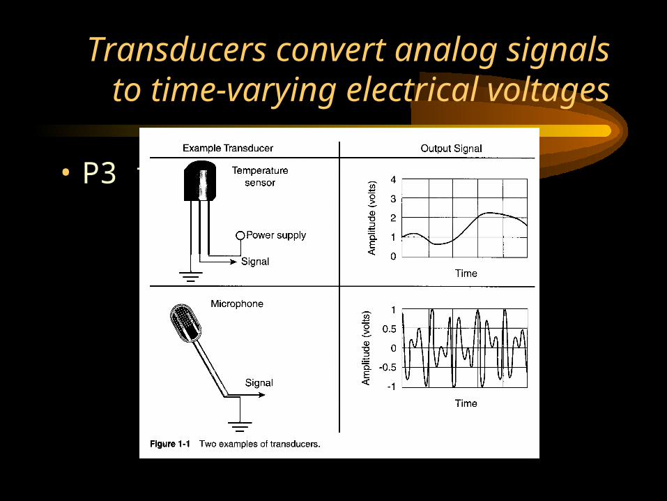
Transducers convert analog signals to time-varying electrical voltages

• P3 fig1-1

Source of analog signals and how they are converted to digital ones

• P20 table 2-1

Nyquist’s Sampling Theorem

• Analog to digital conversion: the analog signal must be sampled at twice the highest frequency component of the signal to avoid distortion.

• Example, for digital audio CD, the sampling rate is 44.1 kHz (based on the highest human audible frequency of around 20 KHz)

Illustration of the Sampling Process

• P4 fig 1-2

Speed of DSP Critical for Real-Time Applications

• Example: sampling rates are 44.1 kHz for audio CD and 48 kHz for digital audio tape (DAT) unit. A DSP CD-to-tape converter must be ready to accept a new sample every 22.6 sec (or 1/44100 sec) from the CD source and produce a new output sample for the DAT every 20.8 sec (1/48000 sec).

Advantages of DSP over analog signal processing (ASP)

• Insensitive to environment• Insensitive to component tolerances• Predictable, repeatable (exact) behavior• Programmability (flexibility)• Size: small than analog counterpart in general• Continued rapid advancement of VLSI technology• Capacity utilization of high BW transmission links• Design tools are available

Applications of DSP

• P8 tab 1-1

Major DSP Vendors

• Analog Devices

• AT&T

• Lucent

• Motorola

• NEC

• Texas Instruments

• Zoran

Fourier Analysis

Fourier Analysis (continued)

Fourier Analysis (continued)

Fourier Analysis (continued)

Fourier Analysis (continued)

Fourier Analysis (continued)

Sinusoidal components (continued): 1 Hz square wave

• P30 fig 2-9, 10

Frequency components of 1 Hz squarewave

Visualization of a signal (Dual Tone Multiple Frequency) in time and frequency domain

• P23 fig 2-3, 4

Fourier series: sinusoidal components of a signal

• P 28 fig 2-7, 8

Filters

• Filter is used to “shape” (selectively change or modify the magnitude and phase of the input signal as a function of frequency) the signals.

Functions of Filters

• Remove noise/interference

• Spectral analysis: analyze the frequency contents of a signal

• Synthesis: generate simple tones to human voice

• …

Types of filters

• Low-pass

• High-pass

• All-pass (amplifier)

• Band-pass

• Band-stop (notch)

• Arbitrary pass-band

• comb

Ideal versus real filter: low-pass

• P67 fig 3-3

The meaning of db or decibel

• P45 tab 2-3

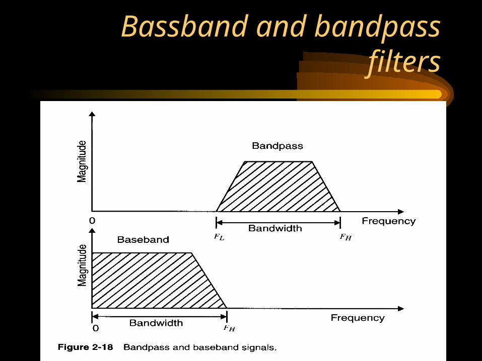
Bassband and bandpass filters

• P38 fig 2-18

Types of filters

• High pass & bandpass

• p70

Types of filters (continued)

• Bandpass & bandstop

• P71 fig 3-8

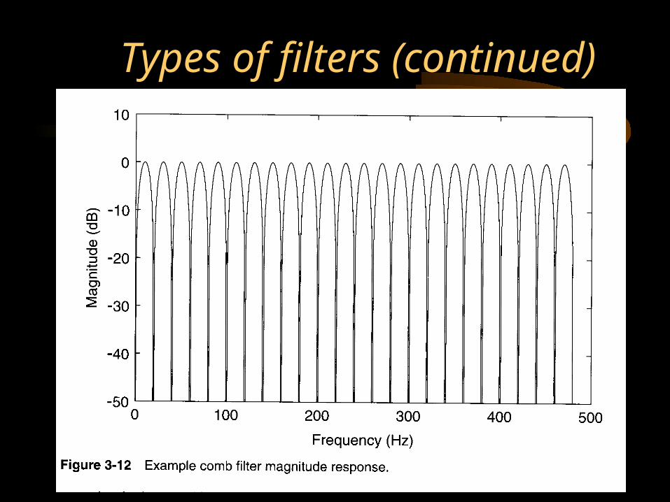
Types of filters (continued)

• Comb filter

• p74 fig 3-12

The characteristics of a real baseband (lowpass) filter

• P41 fig 2-21

Implementation of filters

• Analog filters

• Digital filters: one of the major applications of DSP; offer many advantages over their analog counterpart as described earlier.

Example of filter (notch filter) application: removal of noise

• P66 fig 3-2

Correlation: compare earlier sections of signals with current section (auto-

correlation); special case of filtering.

A typical DSP chip (IC)

• P11 tab 1-2

Limitations of DSP

• Speed: being programmable means 10 to 100 times slower than the hardwired tech.

• Processing: program is simple but needs be done quickly (lots of MAC instructions)

• Precision: use fixed point format with limited precision to save chip space

• Digital signal required more BW than the corresponding analog signal

Visualizing analog signals in time domain

• P22 figs 2-1 & 2-2

Human Speech Spectrum

Describing a system in time domain: the impulse response

• An impulse (math.) excites a system equally at all frequencies.

• P47 fing 2-23

Labeling a system in time domain

• P49 fig 2-25

Impulse response of an elliptical filter

• P48 fig 2-24

The frequency response function

• H(j), where ( or ) is signal frequency; it is also known as the transfer function

• H(j) can be generalized to H(s), the system function, where s = + j, a quantity known as complex frequency. Depending on whether is positive or negative, the signal strength increases or decreases in time, as show in the following example.

Example of complex frequency

• P54 fig 2-30

The complex frequency s-plane

• P57 fig 2-31

Properties of a linear system

• P59 fig 2-33

Poles and zeros of the transfer function

• P85 equations

Poles and zeros (continued)

• P86 equation & fig 3-22

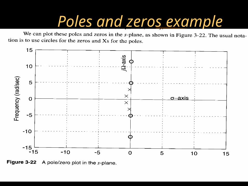
Poles and zeros example

Poles and zeros (continued)

• P88 fig 3-24

Poles and zeros (continued)

• P89 fig 3-25

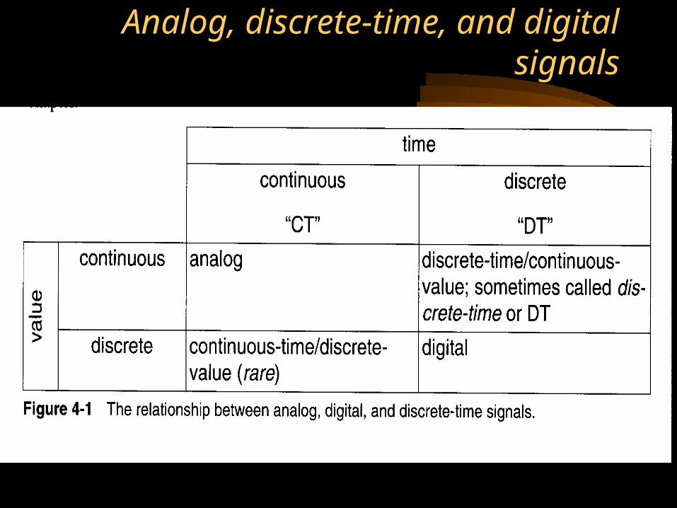
Analog, discrete-time, and digital signals

• P94 fig 4-1

Sampling: 1st step to convert an analog signal to digital one

• Nyquist rate: minimum sampling frequency to avoid undesirable effect (aliasing)

• p96 fig 4-2

Sampling theorem

Sampling theorem (continued)

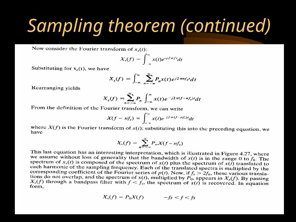
Sampling theorem (continued)

Describing discrete-time system

• H(z): the system or transfer function, where z is the complex frequency in polar coordinates

The polar coordinate and z-plane• P110 fig 4-14

More on H(z) and z-plane• P111 equations, p112 fig 4-15

More on H(z)

Example for a simple system

• P113 fig 4-16

H(z) and the difference equations

• H(s): Laplace transformation of h(t)

• H(z): z-transformation of the DT (discrete time) impulse response of h(n)

• h(t) is a differential equation

• h(n) is described using difference equations, meaning current output of the system is a linear combination of current input samples, past input samples, and past output samples.

The difference equations• General form:

• p116 equation 4-14

• Difference equations can be translated easily into computer programs (run on DSP)

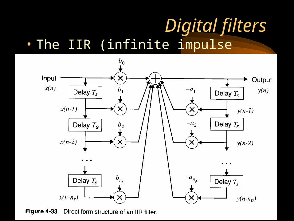
Digital filters• The IIR (infinite impulse response) filter

• p148 fig 4-33

The FIR (finite impulse response) filter

• P149 fig 4-34

IIR versus FIR digital filters

• P152 tab 4-6

DSP implementation of filters

• DSP architecture: