dual memory lstm with dual attention neural network for

sensors

Communication

Dual Memory LSTM with Dual Attention Neural Network forSpatiotemporal Prediction

Teng Li 1 and Yepeng Guan 1,2,*

��

Citation: Li, T.; Guan, Y. Dual

Memory LSTM with Dual Attention

Neural Network for Spatiotemporal

Prediction. Sensors 2021, 21, 4248.

https://doi.org/10.3390/s21124248

Academic Editor: Paweł Pławiak

Received: 23 April 2021

Accepted: 17 June 2021

Published: 21 June 2021

Publisher’s Note: MDPI stays neutral

with regard to jurisdictional claims in

published maps and institutional affil-

iations.

Copyright: © 2021 by the authors.

Licensee MDPI, Basel, Switzerland.

This article is an open access article

distributed under the terms and

conditions of the Creative Commons

Attribution (CC BY) license (https://

creativecommons.org/licenses/by/

4.0/).

1 School of Communication and Information Engineering, Shanghai University, Shanghai 200444, China;[email protected]

2 Key Laboratory of Advanced Display and System Application, Ministry of Education,Shanghai 200072, China

* Correspondence: [email protected]; Tel.: +86-21-6613-7268

Abstract: Spatiotemporal prediction is challenging due to extracting representations being inefficientand the lack of rich contextual dependences. A novel approach is proposed for spatiotemporalprediction using a dual memory LSTM with dual attention neural network (DMANet). A new dualmemory LSTM (DMLSTM) unit is proposed to extract the representations by leveraging differencingoperations between the consecutive images and adopting dual memory transition mechanism. Tomake full use of historical representations, a dual attention mechanism is designed to capturelong-term spatiotemporal dependences by computing the correlations between the current hiddenrepresentations and the historical hidden representations from temporal and spatial dimensions,respectively. Then, the dual attention is embedded into DMLSTM unit to construct a DMANet, whichenables the model with greater modeling power for short-term dynamics and long-term contextualrepresentations. An apparent resistivity map (AR Map) dataset is proposed in this paper. TheB-spline interpolation method is utilized to enhance AR Map dataset and makes apparent resistivitytrend curve continuous derivative in the time dimension. The experimental results demonstrate thatthe developed method has excellent prediction performance by comparisons with some state-of-the-art methods.

Keywords: spatiotemporal prediction; dual memory LSTM; dual attention; historical representations

1. Introduction

Spatiotemporal prediction is learning representations in an unsupervised mannerfrom unlabeled video data and using them to execute a prediction task, which is a typicalcomputer vision task. Currently, the spatiotemporal prediction has been applied to sometasks successfully, such as future prediction of object locations [1,2], anomaly detection [3],and autonomous driving [4]. Deep learning-based models take a leap over the traditionalapproaches because they have learned adequate representations from high-dimensionaldata. Deep learning methods fit perfectly into the spatiotemporal prediction task, whichcould extract spatiotemporal correlations from video data in a self-supervised fashion.However, spatiotemporal prediction is still a challenging task due to the problem of ex-tracting representations inefficiently and the lack of long-term dependencies. For example,Convolutional LSTM (ConvLSTM) [5] has been developed to further extract temporalrepresentations but it ignores spatial representations. Some methods [6,7] have achievedaccurate prediction results, but they cause representation loss. The method of adversarialhas been applied in prediction tasks [8,9]. However, they [8,9] are significantly dependenton the unstable training process.

A novel dual memory LSTM with dual attention neural network (DMANet) has beenproposed for spatiotemporal prediction in this paper to solve the mentioned problems.A dual memory LSTM (DMLSTM) unit based on ConvLSTM [5] has been developed forDMANet to perform spatiotemporal prediction. It can be applied to get representations

Sensors 2021, 21, 4248. https://doi.org/10.3390/s21124248 https://www.mdpi.com/journal/sensors

https://www.mdpi.com/journal/sensors

https://www.mdpi.com

https://doi.org/10.3390/s21124248

https://doi.org/10.3390/s21124248

https://creativecommons.org/

https://creativecommons.org/licenses/by/4.0/

https://creativecommons.org/licenses/by/4.0/

https://doi.org/10.3390/s21124248

https://www.mdpi.com/journal/sensors

https://www.mdpi.com/article/10.3390/s21124248?type=check_update&version=1

Sensors 2021, 21, 4248 2 of 18

of motion by differencing adjacent hidden states or raw images appropriately. Besidesit has dual memory structures to store spatial information and temporal information. Adual attention mechanism is proposed and embedded into the DMLSTM unit to extractlong-term feature dependencies from temporal and spatial dimension, respectively, whichenables the developed model to capture longer complex video dynamics. Compared withthe above spatiotemporal prediction methods, the main contributions of this paper are asfollows. Firstly, a novel DMLSTM unit has been proposed to perform extract represen-tations, which can be applied for spatiotemporal prediction by leveraging differencingoperations between the consecutive images and adopting dual memory transition mech-anism. Secondly, a dual attention mechanism is developed to get the long-term frameinteractions. The long-term frame interactions are captured by computing the correlationbetween the currently hidden representations and the historical hidden representationsfrom the temporal and spatial dimension, respectively. Finally, an important contributionis that the DMANet combines both the advantages. Such architectural design enables themodel with greater modeling power for short-term dynamics and long-term contextualrepresentations. The proposed method is evaluated at some challenging datasets withdifferent methods. It achieves excellent performance by comparison with some state-of-the-art methods. The experimental results show that the proposed method has excellentspatiotemporal prediction performance.

The rest of this article is organized as follows. Related work is discussed in Section 2.The dual memory LSTM with dual attention mechanism is described in Section 3. Exper-imental results and analyses are discussed in Section 4 and followed by conclusions inSection 5.

2. Literature Review

Over the past decade, many methods have been proposed for spatiotemporal predic-tion. Recurrent neural network (RNN) [10] with the long short-term memory (LSTM) [11]has been increasingly applied to prediction task due to its capabilities for learning repre-sentations of video sequence. In recent years, the LSTM framework based on a sequence-to-sequence model [12] has been adapted to video prediction. Still, the accuracy of predictionis limited due to the fact that these framework methods [12] only capture temporal vari-ations. In order to further extract video representations, ConvLSTM [5] replaces fullyconnected operations with convolution operations in recurrent state transitions. A deep-learning-based framework [13] is proposed to reconstruct the missing data to facilitateanalysis with spatiotemporal series. However, it will increase the extra computational costand lower the prediction efficiency. The bijective gated recurrent unit is introduced in [14],which exploits recurrent auto-encoders to predict the next frame in some cases. A multi-output and multi-index of supervised learning [15] method with LSTM [11] is proposed forspatiotemporal prediction, which can model the long-term dynamics. In pursuit of alleviat-ing gradient vanishing, convolutional LSTM extended by [6,7] introduces a zigzag memoryflow and gradient highway unit (GHU). An updated deep learning-based method has beenused for improving prediction capability. A version of ASAP called the “ASAP deep sys-tem”, is proposed in [16]. Optical flow warping and RGB pixel synthesizing algorithms [17]has been exploited to perform spatiotemporal prediction. Memory-in-memory network(MIM) is proposed for prediction task in [18]. Its difference from the above-mentionedrecurrent models is that MIM [18] applies differencing in memory transitions to transformthe time-varying polynomial into a constant, which enables the deterministic componentpredictable. However, these methods [14–18] are still challenging to perform long-termprediction since excessive gate transitions would cause the loss of representations.

In addition to the recurrent models, other models are also employed for spatiotempo-ral prediction. A retrospection network is proposed in [19], which introduces retrospectionloss to push the retrospection frames to be consistent with the observed frames. In order tohandle the imbalance in the data, a neighborhood cleaning algorithm is developed in [20].A random forest algorithm extracts the optimal features to perform prediction task. A

Sensors 2021, 21, 4248 3 of 18

variational autoencoder is adopted to extract nonlinear dynamic features in [21]. Thismodel analyzes the correlations between variables and the relationships between historicalsamples and present samples. A wide-attention module and the deep-composite moduleare utilized in [22] to extract global key features and local key features. However, thesemethods [19–22] depend on local representations to some extent, which cannot get excellentperformance on prediction task. An artificial neural network [23] has been proposed tomodel the unique properties of spatiotemporal data and derives a more powerful modelingcapability to spatiotemporal data. A spatiotemporal prediction system [24] has been devel-oped to focus on spatial modeling and reconstructing the complete spatio-temporal signal.This method shows the effectiveness of modelling coherent spatio-temporal fields. Mixpredneural network has been proposed to model the dynamic pattern and learn appearancerepresentations based on given video frames in [25]. A 3D CNN is utilized into RNNin [26], which extends representations in temporal dimension and makes the memory unitstore better long-term representations. However, convolutional operations [24–26] accountfor short-range intraframe dependencies due to their limited receptive fields and the lackof explicit inter-frame modeling capabilities. The generative adversarial networks [8] isanother approach for spatiotemporal prediction. A conditional variational autoencodermethod has been proposed in [9] by producing future human trajectories conditionedon previous observations and future robot actions. The prediction methods [8,9] aim togenerate less blurry frames, but their performance significantly depends on the unstabletraining process.

A self-attention mechanism is proposed in [27], which can be applied to capture long-range dependencies and has been proved to be effective in aggregating salient featuresamong all spatial positions in computer vision tasks [28–30]. A double attention blockis proposed in [28], which combines the features of the whole space into a compact set,and then adaptively selects and allocates features to each location. In order to exploit thecontextual information more effectively, a crisscross network [29] introduced a crisscrossattention module to get the contextual information of all pixels, which is helpful for visualunderstanding problems. In addition, unlike the multi-scale feature fusion methods, a dualattention network [30] is proposed to combine local features with global dependenciesadaptively. However, they cannot be used to deal with prediction tasks due to the lack ofspatiotemporal dependencies.

In summary, prior prediction models yield different drawbacks. Different from pre-vious work, we design a novel variant of ConvLSTM [5] to store state representationsand extend the attention mechanism in the task of spati otemporal prediction. This ar-chitecture captures rich contextual relationships for better feature representations withintra-class compactness.

Table 1 shows the acronyms used in the paper with a definition about the concept.

Table 1. The acronyms with a definition about the concept.

Acronym Describe

DMANet DMANet is Dual Memory LSTM with Dual Attention Neural Network.DMLSTM DMLSTM is Dual Memory LSTM.

ConvLSTM [5] ConvLSTM is Convolutional LSTM.GHU [7] GHU is Gradient Highway Unit.RNN [10] RNN is Recurrent Neural Network.LSTM [11] LSTM is Long Short-Term Memory.MIM [18] MIM is Memory in Memory Network.

AR AR is Apparent Resistivity.MSE MSE is Mean Square Error.

PSNR PSNR is Peak Signal to Noise Ratio.SSIM [31] SSIM is Structural Similarity Index Measure.

Sensors 2021, 21, 4248 4 of 18

3. DMA Neural Network

A flow chart of DMANet is shown in Figure 1. The representations are extracted fromDMANet given the input frames. The representations indicate prediction result and can beused to predict the next representations.

Sensors 2021, 21, x FOR PEER REVIEW 4 of 18

3. DMA Neural Network

A flow chart of DMANet is shown in Figure 1. The representations are extracted from

DMANet given the input frames. The representations indicate prediction result and can

be used to predict the next representations.

In this section, the details of the DMANet would be given. Firstly, a novel DMLSTM

unit is introduced in Section 3.1. Afterwards, a dual attention mechanism is proposed in

Section 3.2, which enables the model can benefit from the previous relevant representa-

tions. Finally, they are aggregated together to build DMANet for spatiotemporal predic-

tion, which is detailed in Section 3.3.

Figure 1. A flow chart of DMANet in long-term prediction.

3.1. Dual Memory LSTM

It is enlightened by the PredRNN++ [7], which adds more nonlinear layers to increase

the network depth and strengthen the modeling capability for spatial correlations and

temporal dynamics. However, the problem of gradient propagation is becoming more and

more difficult with the increase of network depth, even if GHU [7] alleviates it to a limited

extent. Some work [6,7,14] does not perform well in extracting the representations of spa-

tiotemporal sequences across excessive gate transitions, as it may inescapably cause the

loss of representations. Therefore, long-range spatial dependencies can be captured by

stacked convolution layers. However, the effectiveness of the modeling capability for spa-

tiotemporal dynamics is limited due to the complex layer-to-layer transition.

A new recurrent unit named DMLSTM is developed to perform spatiotemporal pre-

diction to overcome the limitations as mentioned above, as shown in Figure 2. Firstly, an

additional memory unit is added based on ConvLSTM [5]; this unit is used to store spatial

states, which enables the unit to learn more spatiotemporal representations. The novel

transition mechanism is designed by discarding redundant gate structure, such as input

gate. The various nonlinear structure would loss the powerful internal representations in

pixel-level prediction. On the other hand, the representations differencing operations has

been effectively applied to capture the representations of moving objects. Therefore, dif-

ferencing can be used for prediction task to supplement moving objects representation

details. In the DMLSTM unit, the differencing operation is developed to get representa-

tions of motion by differencing adjacent hidden states or raw images, which makes the

unit have a more powerful modeling capability for spatiotemporal dynamics.

Figure 1. A flow chart of DMANet in long-term prediction.

In this section, the details of the DMANet would be given. Firstly, a novel DMLSTMunit is introduced in Section 3.1. Afterwards, a dual attention mechanism is proposed inSection 3.2, which enables the model can benefit from the previous relevant representations.Finally, they are aggregated together to build DMANet for spatiotemporal prediction,which is detailed in Section 3.3.

3.1. Dual Memory LSTM

It is enlightened by the PredRNN++ [7], which adds more nonlinear layers to increasethe network depth and strengthen the modeling capability for spatial correlations andtemporal dynamics. However, the problem of gradient propagation is becoming moreand more difficult with the increase of network depth, even if GHU [7] alleviates it to alimited extent. Some work [6,7,14] does not perform well in extracting the representationsof spatiotemporal sequences across excessive gate transitions, as it may inescapably causethe loss of representations. Therefore, long-range spatial dependencies can be capturedby stacked convolution layers. However, the effectiveness of the modeling capability forspatiotemporal dynamics is limited due to the complex layer-to-layer transition.

A new recurrent unit named DMLSTM is developed to perform spatiotemporalprediction to overcome the limitations as mentioned above, as shown in Figure 2. Firstly, anadditional memory unit is added based on ConvLSTM [5]; this unit is used to store spatialstates, which enables the unit to learn more spatiotemporal representations. The noveltransition mechanism is designed by discarding redundant gate structure, such as inputgate. The various nonlinear structure would loss the powerful internal representationsin pixel-level prediction. On the other hand, the representations differencing operationshas been effectively applied to capture the representations of moving objects. Therefore,differencing can be used for prediction task to supplement moving objects representationdetails. In the DMLSTM unit, the differencing operation is developed to get representationsof motion by differencing adjacent hidden states or raw images, which makes the unit havea more powerful modeling capability for spatiotemporal dynamics.

Sensors 2021, 21, 4248 5 of 18Sensors 2021, 21, x FOR PEER REVIEW 5 of 18

Figure 2. DMLSTM unit.

In the developed DMLSTM unit, [] denotes a concatenation operator, σ is the sigmoid

activation function, tanh is the activation function, ⊙ is the Hadamard product, is ele-

ment-wise addition, and ⊖ is element-wise difference. All vectors are represented in bold.

Ck

t is temporal memory states, and Mk

t is spatial memory states, where k indicates the kth

hidden layer and t denotes time stamp. f

c t, f

m t are forget gate, respectively, where the su-

perscript c and m denote the forget gate are used in temporal memory Ck

t and spatial

memory Mk

t , respectively. it is input gate, gt is input modulation gate, and ot is output one,

respectively. X′ is differential features, rt is input result, and Hk

t denotes the output of

DMLSTM unit, respectively. There are five inputs including the input image features Xt

from encoders, the spatial memory states Mk−1

t from previously hidden layers, the input

image features Xt−1 conveyed from encoders at the last time step, the temporal memory

states Ck

t−1 and the hidden states Hk

t−1 delivered from previous time step, respectively. All

of them are three dimensional tensors in ℝH × W × C, where H and W are spatial size and C

denotes the number of channels, respectively. The update equations of DMLSTM unit are

as follows:

X W X X X bt xx t t- t x= - , +1 (1)

where ∗ is the convolution operation, and [] indicates concatenation of the tensors. W

xx is

the convolutional filters. bx is the bias vector.

Since the moving objects has strong correlations between consecutive images, the

proposed unit is applied to learn the inner dynamics of the movement by taking differ-

encing operations between two consecutive images features. The representations of mov-

ing objects concatenated with frame features Xt to enrich input representations according

to (1).

f W X W H W C bc k kt xf t hf t- cf t- f= σ + + +1 1 (2)

f W X W H W M bm k k-t xf t hf t- mf t f= σ + + +1

1 (3)

i W X W H bkt xi t hi t- i= σ + +1 (4)

g W X W H bkt xg t hg t- g= tanh + +1 (5)

where W

xf, W

hf, W

cf, W

mf, W

xi, W

hi, W

xg, W

hg, W′

xf, and W′

hf are convolutional filters, respec-

tively. bf, bi, bg, and b′

f are the bias vectors, respectively.

Some previous work [6,7] tended to extract the representations across excessive gate

transitions, which would cause the loss of representations. An extra forget gate f

m t and

Figure 2. DMLSTM unit.

In the developed DMLSTM unit, [] denotes a concatenation operator, σ is the sigmoidactivation function, tanh is the activation function, � is the Hadamard product, ⊕ iselement-wise addition, and is element-wise difference. All vectors are represented inbold. Ck

t is temporal memory states, and Mkt is spatial memory states, where k indicates the

kth hidden layer and t denotes time stamp. f c t, f m t are forget gate, respectively, where thesuperscript c and m denote the forget gate are used in temporal memory Ck

t and spatialmemory Mk

t , respectively. it is input gate, gt is input modulation gate, and ot is outputone, respectively. X′ is differential features, rt is input result, and Hk

t denotes the output ofDMLSTM unit, respectively. There are five inputs including the input image features Xtfrom encoders, the spatial memory states Mk−1

t from previously hidden layers, the inputimage features Xt−1 conveyed from encoders at the last time step, the temporal memorystates Ck

t−1 and the hidden states Hkt−1 delivered from previous time step, respectively. All

of them are three dimensional tensors in RH ×W × C, where H and W are spatial size and Cdenotes the number of channels, respectively. The update equations of DMLSTM unit areas follows:

X′t = Wxx ∗ [(Xt −Xt−1), Xt] + bx (1)

where ∗ is the convolution operation, and [] indicates concatenation of the tensors. Wxx isthe convolutional filters. bx is the bias vector.

Since the moving objects has strong correlations between consecutive images, theproposed unit is applied to learn the inner dynamics of the movement by taking differenc-ing operations between two consecutive images features. The representations of movingobjects concatenated with frame features Xt to enrich input representations according to (1).

fct = σ

(Wx f ∗X′t + Wh f ∗Hk

t−1 + Wc f ∗ Ckt−1 + b f

)(2)

fmt = σ

(W′x f ∗X′t + W′h f ∗Hk

t−1 + Wm f ∗Mk−1t + b′f

)(3)

it = σ(

Wxi ∗X′t + Whi ∗Hkt−1 + bi

)(4)

gt = tanh(

Wxg ∗X′t + Whg ∗Hkt−1 + bg

)(5)

where Wx f , Wh f , Wc f , , Wmf , Wxi, Whi, Wxg, Whg, W′x f , and W′h f are convolutional filters,respectively. bf, bi, bg, and b′f are the bias vectors, respectively.

Some previous work [6,7] tended to extract the representations across excessive gatetransitions, which would cause the loss of representations. An extra forget gate f m t andspatial memory states Mk

t are added based on standard ConvLSTM [5], as shown in Figure 2(dotted part). The forget gate f m t is used to forget representations that are not relevant

Sensors 2021, 21, 4248 6 of 18

to Mkt . The spatial memory states Mk

t is used to store spatial representations for furtheruse. The forget gate f c t and f m t, the input gate it and the input modulation gate gt arecontrolled through hidden states Hk

t−1, the differential features X′, previous memory statesCk

t−1 and Mk−1t are gotten according to (2) to (5). Such a transition mechanism extracts

the representations by simpler gate structures to avoid representations loss in massivegates transition.

rt = it·gt (6)

Ckt = fc

t ·Ckt−1 + rt (7)

Mkt = fm

t ·Mk−1t + rt (8)

where ∗is the Hadamard product. These memory states Ckt , Mk

t depends on previousmemory states and input result rt according to (6) to (8), which could make unit obtaincurrent states based on the current learning input and previous states.

ot = tanh(

Wxo ∗X′t + Who ∗Hkt−1 + Wco ∗ Ck

t + Wmo ∗Mkt + bo

)(9)

Hkt = ot·tanh

(W1×1 ∗

[rt, Ck

t , Mkt

])(10)

where Wxo, Who, Wco, and Wmo are convolutional filters, respectively. W1×1 is a 1 × 1

convolutional filter for dimension reduction. bf and bo are the bias vectors, respectively.These memory states Ck

t and Mkt are concatenated with input result rt to get the future

hidden states Hkt through output gate ot according to (9) and (10).

Given an input frame, the goal of our unit is to predict diverse plausible future framesas mentioned above. The unit firstly performs a process of differencing operations betweenthe neighboring frames to produce differential representations containing movementinformation of objects. The differential representations are concatenated with input toenrich spatiotemporal information for further use. In the next stage, the concatenatedrepresentations are fed to the unit to predict future representations. The DMLSTM unitincludes both temporal and spatial memories to storage spatiotemporal representations forfuture prediction. The unit can be applied to generate a candidate of the next frame basedon extracted spatiotemporal representations.

3.2. Dual Attention Mechanism

Spatiotemporal prediction can predict future frames by observing previous represen-tations. However, the prediction model should focus more on historical representationsthat is related to the predicted content. Attention mechanism [27] can capture long-rangedependences between local and global representations in some practical tasks [32,33].Moreover, spatiotemporal prediction is challenging due to the complex dynamics andappearance changes, which requires dependencies on both temporal and spatial domains.A novel variant of attention mechanism named dual attention mechanism is proposed.This architecture captures long-term spatiotemporal interaction from temporal and spa-tial dimensions, respectively, and then the obtained representations are aggregated forfuture prediction.

The dual attention module is shown in Figure 3 including current time stamp hiddenstates Ht ∈ RH ×W × C and historical ones {H1 . . . Ht−1} ∈ Rn × H ×W × C, where H andW are spatial size, C is the number of channels, and n denotes the number of hiddenrepresentations that are concatenated along the temporal dimension, respectively.


Figure 3. Dual attention module.

For the temporal attention module, Ht and {H1…Ht−1} are reshaped into A′ ∈ ℝ1 × HWC

and B′ ∈ ℝn × HWC, respectively. A matrix multiplication is performed between A′ and the

transpose of B′. A softmax function is applied to get the temporal attention map Z ∈ ℝ1 × n:

A Bz

A B

1

1

11

T

j

j Tn

jj=

exp=

exp (11)

where is matrix multiplication operator, the superscript T indicates matrix transpose, A′

1 ∈ ℝ1 × HWC and A′

1 = A′ due to only one hidden states representation, B′

j ∈ ℝ1 × HWC, and z1j

indicates the temporal similarity score between the current time stamp representations

and the previous jth time stamp representations. The more relevant representations of the

two time stamps contribute to greater the weights on attention map.

A matrix multiplication is performed between Z and B′ to get the temporal attention

module output E ∈ ℝ1 × H × W × C as follows:

E z Bn

j jj=

= 11

(12)

Similarly, in the spatial attention module the representations A′′ ∈ ℝHW × C, B′′ ∈ ℝnHW ×

C is reshaped from original representations Ht and {H1…Ht−1}, a matrix multiplication and

softmax function is applied to get the spatial attention map S ∈ ℝHW × nHW:

A Bs

A B

T

i j

ji Tn

i jj=

exp=

exp1

(13)

where A′′

i ∈ ℝ1 × C and B′′

j ∈ ℝ1 × C. sji indicates the spatial similarity between ith position at

the current time stamps representations and the jth position at the historical records ones.

A matrix multiplication is employed between S and B′′ to get the spatial attention

module output F ∈ ℝ1 × H × W × C as follows:

1

F s Bn

ij jj=

= (14)

In pursuit of utilizing the contextual information generated by these two attention

modules and ensuring the dual attention module is stable to be embedded into DMLSTM

unit, these representations are aggregated, and residual mechanism is applied. The aggre-

gated representation Ĥt ∈ ℝ1 × H × W × C is calculated as follows:

H E F Ht t= α + γ + (15)

Figure 3. Dual attention module.

For the temporal attention module, Ht and {H1 . . . Ht−1} are reshaped into A′ ∈R1 × HWC and B′ ∈ Rn × HWC, respectively. A matrix multiplication is performed betweenA′ and the transpose of B′. A softmax function is applied to get the temporal attention mapZ ∈ R1 × n:

z1j =

exp(

A′1 ⊗(

B′j)T)

∑nj=1 exp

(A1′ ⊗

(B′j)T) (11)

where ⊗ is matrix multiplication operator, the superscript T indicates matrix transpose,A′1 ∈R1 × HWC and A1

′ = A′ due to only one hidden states representation, Bj ∈R1 × HWC, andz1j indicates the temporal similarity score between the current time stamp representationsand the previous jth time stamp representations. The more relevant representations of thetwo time stamps contribute to greater the weights on attention map.

A matrix multiplication is performed between Z and B′ to get the temporal attentionmodule output E∈ R1 × H ×W × C as follows:

E =n

∑j=1

z1j ⊗ B′j (12)

Similarly, in the spatial attention module the representations A′′ ∈ RHW × C, B′′ ∈RnHW × C is reshaped from original representations Ht and {H1 . . . Ht−1}, a matrix multi-plication and softmax function is applied to get the spatial attention map S ∈ RHW × nHW:

sji =

exp(

A′′i ⊗(

B′′j)T)

∑nj=1 exp

(A′′i ⊗

(B′′j)T) (13)

where A′′i ∈ R1 × C and B′′

j ∈ R1 × C. sji indicates the spatial similarity between ith positionat the current time stamps representations and the jth position at the historical records ones.

A matrix multiplication is employed between S and B′′ to get the spatial attentionmodule output F ∈ R1 × H ×W × C as follows:

F =n

∑j=1

sij ⊗ B′′j (14)

In pursuit of utilizing the contextual information generated by these two attentionmodules and ensuring the dual attention module is stable to be embedded into DML-

Sensors 2021, 21, 4248 8 of 18

STM unit, these representations are aggregated, and residual mechanism is applied. Theaggregated representation Ht ∈ R1 × H ×W × C is calculated as follows:

Ht = αE + γF + Ht (15)

where α and γ is used to weight the contribution of E and F, respectively. Both α and γwould be discussed later.

The dual attention memory module is embedded into the DMLSTM unit to constructthe DMA unit, as illustrated in Figure 4. The operations in DM-LSTM are followed byEquations (1)–(10). The DMLSTM unit can be applied to characterize the features ofinput frames, which is discussed later. The operations in Dual Attention are followedby Equations (11)–(15). The dual attention module can adaptively memorize the longerdependences by aggregating long-term contextual information.


where α and γ is used to weight the contribution of E and F, respectively. Both α and γ

would be discussed later.

The dual attention memory module is embedded into the DMLSTM unit to construct

the DMA unit, as illustrated in Figure 4. The operations in DM-LSTM are followed by

Equations (1)–(10). The DMLSTM unit can be applied to characterize the features of input

frames, which is discussed later. The operations in Dual Attention are followed by Equa-

tions (11)–(15). The dual attention module can adaptively memorize the longer depend-

ences by aggregating long-term contextual information.

Figure 4. DMA unit.

3.3. DMANet

In order to design a powerful spatiotemporal prediction model, a DMANet is built

by stacking L DMA units to extract highly abstract representations. In addition, the GHU

[7] is injected between the 1st and 2nd layers to alleviate the problem of vanishing gradi-

ent. The prediction result is generated by mapping the output representations back to the

pixel value space. A schematic of the developed DMANet is shown in Figure 5. The cal-

culations of the entire model are as follows (for 3 ≤ k ≤ L):

ˆ ˆH M C X X H C M Lt t t t t- t- t- t, , = , , , ,1 1 1 1 1

1 1 1DMA (16)

ˆZ Z Ht t- t= ( , )11GHU (17)

ˆ ˆ ˆH , M ,C = Z , H , H ,C , Mt t t t t- t t- t2 2 2 1 2 2 1

1 -1 1DMA (18)

ˆ ˆ ˆ ˆH M C H H H C Mk k k k- k- k k k-t t t t t- t- t- t, , = , , , ,1 1 1

1 1 1DMA (19)

where the superscript L denotes the number of DMANet layers, which would be dis-

cussed later. The subscript t denotes the time stamp. Zt denotes hidden states from GHU

[7], which models long-term dynamics according to (17).

The input frames Xt are fed into the bottom layer to predict future ones. The hidden

representations Ĥt horizontally and vertically transmitted. The diagonal arrows denote

the forward directions of Xt or Ĥt for differential modeling. The memory states Ck

t−1 hori-

zontally conveyed from t−1 stamp to t one. Ck

t−1 is used to store temporal representations

at t−1 stamp. The memory states Mk−1

t vertically delivered from k−1 layer to k one. Mk−1

t is

used to store spatial representations at k−1 layer. Specially, the memory states ML

t would

be updated in a zigzag direction at top layer, as M1

t = ML

t−1, in which the DMA units can be

applied to get more sufficient representations of past for further prediction. The final out-

put Xt+1 indicates prediction result and can be used to predict next representations.

Since this structure utilizes several state transitions paths to deliver the extracted rep-

resentations which is necessary for spatiotemporal prediction, the stacked DMANet could

be applied to extract more high-level representations from the bottom layer upwards. Be-

sides diagonal state transition paths are exploited to extract motion representations of

moving objects by differencing operations. The developed DMANet can be applied to get

both spatiotemporal representations and capture the longer dependences by DMLSTM

unit and dual attention module, respectively.

Figure 4. DMA unit.

3.3. DMANet

In order to design a powerful spatiotemporal prediction model, a DMANet is built bystacking L DMA units to extract highly abstract representations. In addition, the GHU [7]is injected between the 1st and 2nd layers to alleviate the problem of vanishing gradient.The prediction result is generated by mapping the output representations back to the pixelvalue space. A schematic of the developed DMANet is shown in Figure 5. The calculationsof the entire model are as follows (for 3 ≤ k ≤ L):

H1t , M1

t , C1t = DMA

(Xt, Xt−1, H1

t−1, C1t−1, ML

t

)(16)

Zt = GHU(Zt−1, H1t ) (17)

H2t , M2

t , C2t = DMA

(Zt, H1

t−1, H2t−1, C2

t−1, M1t

)(18)

Hkt , Mk

t , Ckt = DMA

(Hk−1

t , Hk−1t−1 , Hk

t−1, Ckt−1, Mk−1

t

)(19)

where the superscript L denotes the number of DMANet layers, which would be discussedlater. The subscript t denotes the time stamp. Zt denotes hidden states from GHU [7],which models long-term dynamics according to (17).

The input frames Xt are fed into the bottom layer to predict future ones. The hiddenrepresentations Ht horizontally and vertically transmitted. The diagonal arrows denote theforward directions of Xt or Ht for differential modeling. The memory states Ck

t−1 horizon-tally conveyed from t−1 stamp to t one. Ck

t−1 is used to store temporal representations att−1 stamp. The memory states Mk−1

t vertically delivered from k−1 layer to k one. Mk−1t is

used to store spatial representations at k−1 layer. Specially, the memory states MLt would

be updated in a zigzag direction at top layer, as M1t = ML

t−1 in which the DMA units canbe applied to get more sufficient representations of past for further prediction. The finaloutput Xt+1 indicates prediction result and can be used to predict next representations.


Figure 5. DMANet.

3.4. Training Method

L1 and L2 losses has been widely used for prediction task [6,7]. L1 loss can alleviate

blurry prediction results. L2 loss can make the model converge faster. For training, the

loss function used is the sum of L1 and L2 terms to optimize DMANet and they are com-

bined as follow:

ˆ ˆ ˆ

n 2

i i i ii=1

1L , = Y - Y + Y - Y

2Y Y (20)

where |·| is absolute value function operator; n is the number of prediction frames. Ŷ and

Y denote the prediction results and the ground truth, respectively. Ŷi and Yi are the ith

element of Ŷ and Y, respectively.

4. Experiments

4.1. Dataset and Implements

All experiments are implemented using TensorFlow on a Linux machine equipped

with an Intel Xeon E5-2683 v3 CPU and Nvidia GeForce GTX 1070Ti GPU. In order to

verify the performance of the proposed method, the experiments are performed on some

challenging datasets. To test the performance of the developed method, some datasets are

selected as follows. Moving MNIST [34] is constructed by two digits moving inde-

pendently around the frame. The digits are placed initially at random locations. The

movement of digits is irregularly, which makes model difficult to maintain the accuracy

of predictions. Moving MNIST [34] contains 10,000 sequences for training set and 5000

sequences for test set. Each sequence consists of 20 frames with 10 for inputs and 10 for

prediction results, and each frames size are 64 × 64 × 1.

KITTI [35] is another tested dataset, which is taken by the vehicle-mounted camera

on a car driving around an urban environment. The “City”, “Residential”, and “Road”

categories are selected for training. To further assess the performance of the developed

method with robust representation, the trained model is tested on the Caltech [36], which

is another car-mounted camera video dataset. These datasets describe rich temporal dy-

namics of multiple moving objects and presents another level of difficulty for spatiotem-

poral prediction. The model evaluated on the Caltech [36] by predicting 10 future frames

Figure 5. DMANet.

Since this structure utilizes several state transitions paths to deliver the extractedrepresentations which is necessary for spatiotemporal prediction, the stacked DMANetcould be applied to extract more high-level representations from the bottom layer upwards.Besides diagonal state transition paths are exploited to extract motion representations ofmoving objects by differencing operations. The developed DMANet can be applied to getboth spatiotemporal representations and capture the longer dependences by DMLSTMunit and dual attention module, respectively.

3.4. Training Method

L1 and L2 losses has been widely used for prediction task [6,7]. L1 loss can alleviateblurry prediction results. L2 loss can make the model converge faster. For training, the lossfunction used is the sum of L1 and L2 terms to optimize DMANet and they are combinedas follow:

L(Y, Y

)=

n

∑i=1

(∣∣Yi −Yi∣∣+ 1

2

∣∣Yi −Yi∣∣2) (20)

where |·| is absolute value function operator; n is the number of prediction frames. Y andY denote the prediction results and the ground truth, respectively. Yi and Yi are the ithelement of Y and Y, respectively.

4. Experiments4.1. Dataset and Implements

All experiments are implemented using TensorFlow on a Linux machine equippedwith an Intel Xeon E5-2683 v3 CPU and Nvidia GeForce GTX 1070Ti GPU. In order toverify the performance of the proposed method, the experiments are performed on somechallenging datasets. To test the performance of the developed method, some datasets areselected as follows. Moving MNIST [34] is constructed by two digits moving independentlyaround the frame. The digits are placed initially at random locations. The movement ofdigits is irregularly, which makes model difficult to maintain the accuracy of predictions.Moving MNIST [34] contains 10,000 sequences for training set and 5000 sequences for testset. Each sequence consists of 20 frames with 10 for inputs and 10 for prediction results,and each frames size are 64 × 64 × 1.

Sensors 2021, 21, 4248 10 of 18

KITTI [35] is another tested dataset, which is taken by the vehicle-mounted cameraon a car driving around an urban environment. The “City”, “Residential”, and “Road”categories are selected for training. To further assess the performance of the developedmethod with robust representation, the trained model is tested on the Caltech [36], which isanother car-mounted camera video dataset. These datasets describe rich temporal dynamicsof multiple moving objects and presents another level of difficulty for spatiotemporalprediction. The model evaluated on the Caltech [36] by predicting 10 future frames given 10previous frames. The training set consisted of 40,312 sequences. The tested set contains 3631sequences. All sequences include 20 frames, which are center cropped and downsampledto 128 × 160 × 3.

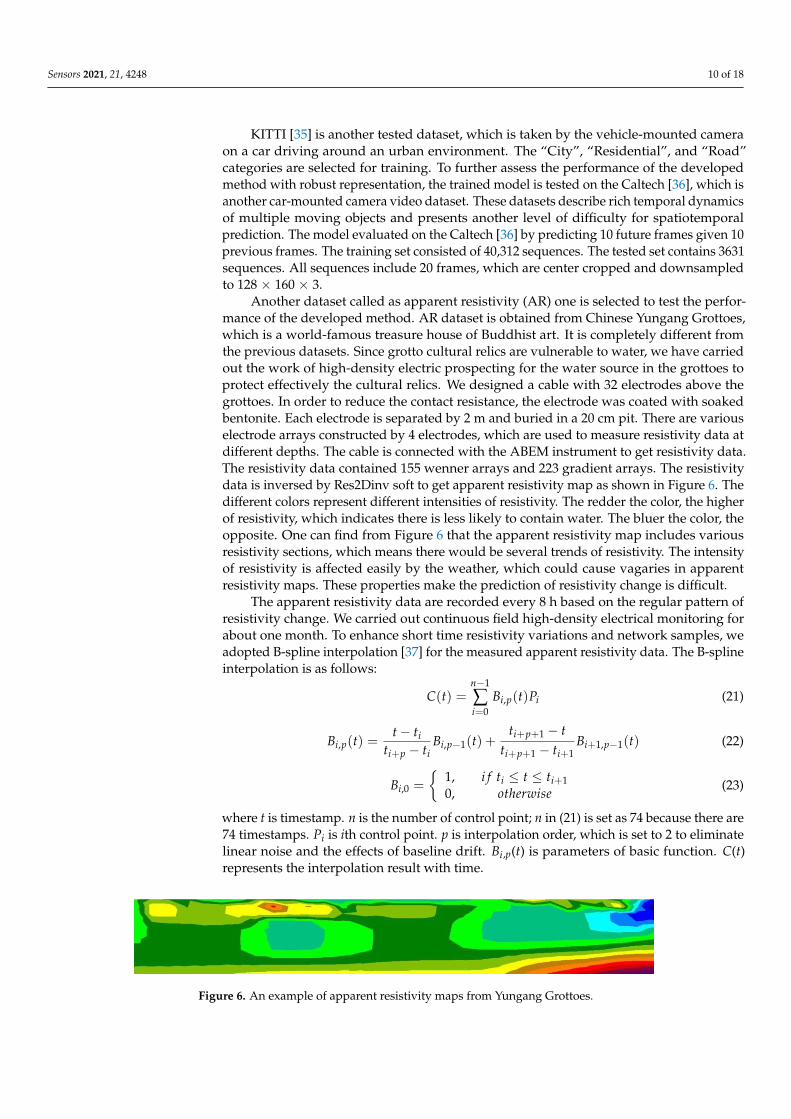
Another dataset called as apparent resistivity (AR) one is selected to test the perfor-mance of the developed method. AR dataset is obtained from Chinese Yungang Grottoes,which is a world-famous treasure house of Buddhist art. It is completely different fromthe previous datasets. Since grotto cultural relics are vulnerable to water, we have carriedout the work of high-density electric prospecting for the water source in the grottoes toprotect effectively the cultural relics. We designed a cable with 32 electrodes above thegrottoes. In order to reduce the contact resistance, the electrode was coated with soakedbentonite. Each electrode is separated by 2 m and buried in a 20 cm pit. There are variouselectrode arrays constructed by 4 electrodes, which are used to measure resistivity data atdifferent depths. The cable is connected with the ABEM instrument to get resistivity data.The resistivity data contained 155 wenner arrays and 223 gradient arrays. The resistivitydata is inversed by Res2Dinv soft to get apparent resistivity map as shown in Figure 6. Thedifferent colors represent different intensities of resistivity. The redder the color, the higherof resistivity, which indicates there is less likely to contain water. The bluer the color, theopposite. One can find from Figure 6 that the apparent resistivity map includes variousresistivity sections, which means there would be several trends of resistivity. The intensityof resistivity is affected easily by the weather, which could cause vagaries in apparentresistivity maps. These properties make the prediction of resistivity change is difficult.

The apparent resistivity data are recorded every 8 h based on the regular pattern ofresistivity change. We carried out continuous field high-density electrical monitoring forabout one month. To enhance short time resistivity variations and network samples, weadopted B-spline interpolation [37] for the measured apparent resistivity data. The B-splineinterpolation is as follows:

C(t) =n−1

∑i=0

Bi,p(t)Pi (21)

Bi,p(t) =t− ti

ti+p − tiBi,p−1(t) +

ti+p+1 − tti+p+1 − ti+1

Bi+1,p−1(t) (22)

Bi,0 =

{1,0,

i f ti ≤ t ≤ ti+1otherwise

(23)

where t is timestamp. n is the number of control point; n in (21) is set as 74 because there are74 timestamps. Pi is ith control point. p is interpolation order, which is set to 2 to eliminatelinear noise and the effects of baseline drift. Bi,p(t) is parameters of basic function. C(t)represents the interpolation result with time.


given 10 previous frames. The training set consisted of 40,312 sequences. The tested set

contains 3631 sequences. All sequences include 20 frames, which are center cropped and

downsampled to 128 × 160 × 3.

Another dataset called as apparent resistivity (AR) one is selected to test the perfor-

mance of the developed method. AR dataset is obtained from Chinese Yungang Grottoes,

which is a world-famous treasure house of Buddhist art. It is completely different from

the previous datasets. Since grotto cultural relics are vulnerable to water, we have carried

out the work of high-density electric prospecting for the water source in the grottoes to

protect effectively the cultural relics. We designed a cable with 32 electrodes above the

grottoes. In order to reduce the contact resistance, the electrode was coated with soaked

bentonite. Each electrode is separated by 2 m and buried in a 20 cm pit. There are various

electrode arrays constructed by 4 electrodes, which are used to measure resistivity data at

different depths. The cable is connected with the ABEM instrument to get resistivity data.

The resistivity data contained 155 wenner arrays and 223 gradient arrays. The resistivity

data is inversed by Res2Dinv soft to get apparent resistivity map as shown in Figure 6.

The different colors represent different intensities of resistivity. The redder the color, the

higher of resistivity, which indicates there is less likely to contain water. The bluer the

color, the opposite. One can find from Figure 6 that the apparent resistivity map includes

various resistivity sections, which means there would be several trends of resistivity. The

intensity of resistivity is affected easily by the weather, which could cause vagaries in

apparent resistivity maps. These properties make the prediction of resistivity change is

difficult.

Figure 6. An example of apparent resistivity maps from Yungang Grottoes.

The apparent resistivity data are recorded every 8 h based on the regular pattern of

resistivity change. We carried out continuous field high-density electrical monitoring for

about one month. To enhance short time resistivity variations and network samples, we

adopted B-spline interpolation [37] for the measured apparent resistivity data. The B-

spline interpolation is as follows:

n-

i,p ii=0

C t = B t P1

(21)

i+p+i

i,p i,p-1 i+ ,p-

i+p i i+p+ i+

t - tt - tB t = B t + B t

t - t t - t

1

1 1

1 1

(22)

i i+

i,0

, if t t tB =

, otherwise11

0 (23)

where t is timestamp. n is the number of control point; n in (21) is set as 74 because there

are 74 timestamps. Pi is ith control point. p is interpolation order, which is set to 2 to elim-

inate linear noise and the effects of baseline drift. Bi,p(t) is parameters of basic function.

C(t) represents the interpolation result with time.

The produced B-spline curve as shown in Figure 7. The B-spline interpolation [37] is

used to enhance apparent resistivity map data to be a continuous derivative curve for

better matching the data requirement. One can find that the curve perfectly fits the change

of control point, which indicates that the cumulative change of resistivity can be repre-

sented by the B-spline interpolation [37]. Each frame is captured at an interval of 20 min.

Figure 6. An example of apparent resistivity maps from Yungang Grottoes.

Sensors 2021, 21, 4248 11 of 18

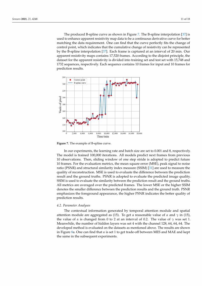
The produced B-spline curve as shown in Figure 7. The B-spline interpolation [37] isused to enhance apparent resistivity map data to be a continuous derivative curve for bettermatching the data requirement. One can find that the curve perfectly fits the change ofcontrol point, which indicates that the cumulative change of resistivity can be representedby the B-spline interpolation [37]. Each frame is captured at an interval of 20 min. Ourapparent resistivity maps contains 17,520 frames. According to the disjoint principle, thedataset for the apparent resistivity is divided into training set and test set with 15,748 and1732 sequences, respectively. Each sequence contains 10 frames for input and 10 frames forprediction results.


Our apparent resistivity maps contains 17,520 frames. According to the disjoint principle,

the dataset for the apparent resistivity is divided into training set and test set with 15,748

and 1732 sequences, respectively. Each sequence contains 10 frames for input and 10

frames for prediction results.

Figure 7. The example of B-spline curve.

In our experiments, the learning rate and batch size are set to 0.001 and 8, respec-

tively. The model is trained 100,000 iterations. All models predict next frames from previ-

ous 10 observations. Then, sliding window of one step stride is adopted to predict future

10 frames. For the evaluation metrics, the mean square error (MSE), peak signal to noise

ratio (PSNR) and structural similarity index measure (SSIM) [31] are used to measure the

quality of reconstruction. MSE is used to evaluate the difference between the prediction

result and the ground truths. PSNR is adopted to evaluate the predicted image quality.

SSIM is used to evaluate the similarity between the prediction result and the ground

truths. All metrics are averaged over the predicted frames. The lower MSE or the higher

SSIM denotes the smaller difference between the prediction results and the ground truth.

PSNR emphasizes the foreground appearance, the higher PSNR indicates the better qual-

ity of prediction results.

4.2. Parameter Analyses

The contextual information generated by temporal attention module and spatial at-

tention module are aggregated as (15). To get a reasonable value of α and γ in (15), the

value of α is changed from 0 to 2 at an interval of 0.2. The value of γ was set 1. Meanwhile,

the number of hidden layers was set 4 with the channel 128, 64, 64, 64. The developed

method is evaluated on the datasets as mentioned above. The results are shown in Figure

8a. One can find that α is set 1 to get trade-off between MES and MAE and kept the same

in the subsequent experiments.

Similarly, the value of γ is changed from 0 to 2 at an interval of 0.2. The value of α

was set 1. The number of hidden layers and channel as mentioned above. The experi-

mental results are shown in Figure 8b. When γ is 1, the prediction performance is the best.

In the subsequent experiments, γ is set as 1 and keep the same.

Figure 7. The example of B-spline curve.

In our experiments, the learning rate and batch size are set to 0.001 and 8, respectively.The model is trained 100,000 iterations. All models predict next frames from previous10 observations. Then, sliding window of one step stride is adopted to predict future10 frames. For the evaluation metrics, the mean square error (MSE), peak signal to noiseratio (PSNR) and structural similarity index measure (SSIM) [31] are used to measure thequality of reconstruction. MSE is used to evaluate the difference between the predictionresult and the ground truths. PSNR is adopted to evaluate the predicted image quality.SSIM is used to evaluate the similarity between the prediction result and the ground truths.All metrics are averaged over the predicted frames. The lower MSE or the higher SSIMdenotes the smaller difference between the prediction results and the ground truth. PSNRemphasizes the foreground appearance, the higher PSNR indicates the better quality ofprediction results.

4.2. Parameter Analyses

The contextual information generated by temporal attention module and spatialattention module are aggregated as (15). To get a reasonable value of α and γ in (15),the value of α is changed from 0 to 2 at an interval of 0.2. The value of γ was set 1.Meanwhile, the number of hidden layers was set 4 with the channel 128, 64, 64, 64. Thedeveloped method is evaluated on the datasets as mentioned above. The results are shownin Figure 8a. One can find that α is set 1 to get trade-off between MES and MAE and keptthe same in the subsequent experiments.


Figure 8. Prediction performance in different αs (a) and γs (b) at different datasets from top to bottom, left to right, re-

spectively.

The number of hidden channels is another factor in representations extraction for

spatiotemporal prediction. Low-level representations have a strong impact on the predic-

tion result of DMANet. The representations may not be extracted at all, or the network

performance is poor if the number of hidden channels is too small. However, if the num-

ber of channels in the hidden layer is too great, the error would be increased, and the

training time of the whole network model would be prolonged. In order to get an optimal

number of hidden channels in bottom layer, the number of hidden channels is changed

from 64 to 256 at an interval of 64. Then, the number of hidden layers is fixed to 4 and the

number of channels in all layers except the bottom layer is set to 64. The comparison re-

sults are shown in Figure 9. It can be seen from Figure 9 that the number of channels in

the bottom layer has significant influence on the prediction performance. When the num-

ber of channels in bottom layer is 128, the prediction performance is the best. Then, pre-

diction performance decreases with channel increasing. Therefore, the number of hidden

channels in bottom layer is set as 128 and kept the same in the subsequent experiments.

Figure 9. Prediction performance under different number of channels in bottom layer.

On the other hand, DMANet is constructed by stack L DMA units. Deeper networks

can capture spatiotemporal representations more effectively. To get a reasonable number

of hidden layers for DMANet, the number of hidden layers is changed from 2 to 9 at an

Figure 8. Prediction performance in different αs (a) and γs (b) at different datasets from top to bottom, left to right,respectively.

Similarly, the value of γ is changed from 0 to 2 at an interval of 0.2. The value of α wasset 1. The number of hidden layers and channel as mentioned above. The experimentalresults are shown in Figure 8b. When γ is 1, the prediction performance is the best. In thesubsequent experiments, γ is set as 1 and keep the same.

The number of hidden channels is another factor in representations extraction forspatiotemporal prediction. Low-level representations have a strong impact on the predic-tion result of DMANet. The representations may not be extracted at all, or the networkperformance is poor if the number of hidden channels is too small. However, if the numberof channels in the hidden layer is too great, the error would be increased, and the trainingtime of the whole network model would be prolonged. In order to get an optimal numberof hidden channels in bottom layer, the number of hidden channels is changed from 64 to256 at an interval of 64. Then, the number of hidden layers is fixed to 4 and the number ofchannels in all layers except the bottom layer is set to 64. The comparison results are shownin Figure 9. It can be seen from Figure 9 that the number of channels in the bottom layerhas significant influence on the prediction performance. When the number of channels inbottom layer is 128, the prediction performance is the best. Then, prediction performancedecreases with channel increasing. Therefore, the number of hidden channels in bottomlayer is set as 128 and kept the same in the subsequent experiments.

Sensors 2021, 21, 4248 13 of 18


Figure 8. Prediction performance in different αs (a) and γs (b) at different datasets from top to bottom, left to right, re-

spectively.

The number of hidden channels is another factor in representations extraction for

spatiotemporal prediction. Low-level representations have a strong impact on the predic-

tion result of DMANet. The representations may not be extracted at all, or the network

performance is poor if the number of hidden channels is too small. However, if the num-

ber of channels in the hidden layer is too great, the error would be increased, and the

training time of the whole network model would be prolonged. In order to get an optimal

number of hidden channels in bottom layer, the number of hidden channels is changed

from 64 to 256 at an interval of 64. Then, the number of hidden layers is fixed to 4 and the

number of channels in all layers except the bottom layer is set to 64. The comparison re-

sults are shown in Figure 9. It can be seen from Figure 9 that the number of channels in

the bottom layer has significant influence on the prediction performance. When the num-

ber of channels in bottom layer is 128, the prediction performance is the best. Then, pre-

diction performance decreases with channel increasing. Therefore, the number of hidden

channels in bottom layer is set as 128 and kept the same in the subsequent experiments.


On the other hand, DMANet is constructed by stack L DMA units. Deeper networks

can capture spatiotemporal representations more effectively. To get a reasonable number

of hidden layers for DMANet, the number of hidden layers is changed from 2 to 9 at an


On the other hand, DMANet is constructed by stack L DMA units. Deeper networkscan capture spatiotemporal representations more effectively. To get a reasonable number ofhidden layers for DMANet, the number of hidden layers is changed from 2 to 9 at an intervalof 1. The proposed model is evaluated on the datasets as mentioned above with differentnumber of layers. The comparison results are shown in Figure 10. One can find that withthe increase of the number of hidden layers, the prediction performance increases graduallyat first. When the number of hidden layers is 4, the prediction performance is the best.Then, the prediction performance decreases gradually with the increase of hidden layers.The reason is that the prediction model can be further extract video representations withthe increase of the number of hidden layers, but excessively layers may inevitably lead totraining difficulty and a loss of information representations. In the subsequent experiments,the number of DMANet layers is set 4 and kept same in the subsequent experiments.


interval of 1. The proposed model is evaluated on the datasets as mentioned above with

different number of layers. The comparison results are shown in Figure 10. One can find

that with the increase of the number of hidden layers, the prediction performance in-

creases gradually at first. When the number of hidden layers is 4, the prediction perfor-

mance is the best. Then, the prediction performance decreases gradually with the increase

of hidden layers. The reason is that the prediction model can be further extract video rep-

resentations with the increase of the number of hidden layers, but excessively layers may

inevitably lead to training difficulty and a loss of information representations. In the sub-

sequent experiments, the number of DMANet layers is set 4 and kept same in the subse-

quent experiments.

Figure 10. Prediction performance under different number of hidden layers.

4.3. DMLSTM Unit and the Dual Attention Mechanism Evaluation

To assess the effectiveness of both DMLSTM unit and the dual attention mechanism,

four variants of our model are applied including: PredRNN++ [7] is taken as a baseline

model. DMLSTM is consisted of stacking 4-layer DMLSTM units. DA-PredRNN++ is

PredRNN++ [7] with the dual attention. DMANet is built by stacking 4-layer DMA units.

Some results are given in Table 2.

Table 2. Ablation study in different methods.

Dataset Moving MNIST [34] Caltech [36] AR Map

MSE PSNR SSIM MSE PSNR SSIM MSE PSNR SSIM

PredRNN++ [7] 46.51 20.22 0.88 479.26 19.57 0.71 16.54 32.35 0.91

DMLSTM 49.66 20.53 0.90 437.65 20.14 0.72 18.45 32.78 0.90

DA-PredRNN++ 46.23 20.86 0.90 442.22 19.75 0.73 15.17 32.56 0.91

DMANet 44.36 21.36 0.91 423.98 20.46 0.74 13.14 33.16 0.92

One can find from Table 2 that the developed DMANet achieves the best result on all

datasets by comparisons. The reason is that DMANet adopts a new transition mechanism

and differencing operations, which could more effectively extract the representations of

spatiotemporal sequences and the motion trend of objects. In addition, DMANet is opti-

mal as the dual attention mechanism could make full use of the spatiotemporal contextual

dependences. The attention mechanism is utilized to obtain global representations, which

is a practical way to improve prediction performance. The experiment results demonstrate

that the proposed DMLSTM unit and dual attention mechanism has excellent prediction

performance.

4.4. Comparisons with Some State-of-the-Art Methods

In order to further evaluate whether the proposed method is effective to perform

prediction, the proposed method has been compared with some methods [6,7,14,18].

PredRNN [6] and PredRNN++ [7] introduced a zigzag memory flow and GHU to allevi-

ating gradient vanishing. FRNN [14] is an architecture based on recurrent convolutional

Figure 10. Prediction performance under different number of hidden layers.

4.3. DMLSTM Unit and the Dual Attention Mechanism Evaluation

To assess the effectiveness of both DMLSTM unit and the dual attention mechanism,four variants of our model are applied including: PredRNN++ [7] is taken as a baselinemodel. DMLSTM is consisted of stacking 4-layer DMLSTM units. DA-PredRNN++ isPredRNN++ [7] with the dual attention. DMANet is built by stacking 4-layer DMA units.Some results are given in Table 2.

One can find from Table 2 that the developed DMANet achieves the best result on alldatasets by comparisons. The reason is that DMANet adopts a new transition mechanismand differencing operations, which could more effectively extract the representations ofspatiotemporal sequences and the motion trend of objects. In addition, DMANet is optimalas the dual attention mechanism could make full use of the spatiotemporal contextualdependences. The attention mechanism is utilized to obtain global representations, whichis a practical way to improve prediction performance. The experiment results demonstratethat the proposed DMLSTM unit and dual attention mechanism has excellent predictionperformance.

Sensors 2021, 21, 4248 14 of 18

Table 2. Ablation study in different methods.

DatasetMoving MNIST [34] Caltech [36] AR Map


PredRNN++ [7] 46.51 20.22 0.88 479.26 19.57 0.71 16.54 32.35 0.91DMLSTM 49.66 20.53 0.90 437.65 20.14 0.72 18.45 32.78 0.90

DA-PredRNN++ 46.23 20.86 0.90 442.22 19.75 0.73 15.17 32.56 0.91DMANet 44.36 21.36 0.91 423.98 20.46 0.74 13.14 33.16 0.92

4.4. Comparisons with Some State-of-the-Art Methods

In order to further evaluate whether the proposed method is effective to performprediction, the proposed method has been compared with some methods [6,7,14,18]. Pre-dRNN [6] and PredRNN++ [7] introduced a zigzag memory flow and GHU to alleviatinggradient vanishing. FRNN [14] is an architecture based on recurrent convolutional autoen-coders, which can address the network capacity and error propagation problems for futureprediction. MIM [18] captures higher orders of non-stationarity to facilitate non-stationaritymodeling and make the future sequence more predictable. The parameter used are allthose recommended by the authors in [6,7,14,18], respectively. Some comparison resultsas follows.

Figures 11–13 shows whisker plot comparisons at the chose datasets, which are usedto reflect the distribution characteristics of the prediction results. It can be seen fromFigures 11–13 that the developed method achieves the best performance with statisticalsignificance among the investigated methods.


autoencoders, which can address the network capacity and error propagation problems

for future prediction. MIM [18] captures higher orders of non-stationarity to facilitate non-

stationarity modeling and make the future sequence more predictable. The parameter

used are all those recommended by the authors in [6,7,14,18], respectively. Some compar-

ison results as follows.

Figures 11–13 shows whisker plot comparisons at the chose datasets, which are used

to reflect the distribution characteristics of the prediction results. It can be seen from Fig-

ures 11–13 that the developed method achieves the best performance with statistical sig-

nificance among the investigated methods.

Figure 11. Whisker plot comparisons of the different models at the Moving MNIST [34].

Figure 12. Whisker plot comparisons of the different models at the Caltech [36].

Figure 13. Whisker plot comparisons of the different models at the AR Map.

Figures 14–16 shows frame-by-frame quantitative experiments for the 10 frames at

the chose datasets. It can be seen that the developed method has the best performance

among the investigated methods with the lowest MSE, both the highest PSNR and SSIM

at each frame.


















at each frame.


Sensors 2021, 21, 4248 15 of 18

















at each frame.


Figures 14–16 shows frame-by-frame quantitative experiments for the 10 frames atthe chose datasets. It can be seen that the developed method has the best performanceamong the investigated methods with the lowest MSE, both the highest PSNR and SSIM ateach frame.


Figure 14. Frame-by-frame quantitative results for the 10 frames at the Moving MNIST [34].

Figure 15. Frame-by-frame quantitative results for the 10 frames at the Caltech [36].

Figure 16. Frame-by-frame quantitative results for the 10 frames at the AR Map.

To further demonstrate that the proposed method has the best performance, we have

computed results as mean ± standard deviation in Table 3. One can find from Table 3 that

the proposed method has the best performance among the investigated methods. Some

reasons are as follows. A bijective mapping method is utilized to share states between

encoder and decoder in [14], bijective mapping could extract representations from low

dimension to high dimension. However, the relationship between the consecutive repre-

sentations is not considered, which is important to dynamic objects modeling. PredRNN

[6] is not able to forecast accurately due to vanishing gradient and inefficient representa-

tions. The dynamic regions are blurred, and the action of objects is uncertain due to inef-

ficient representations. The problem of vanishing gradient indicates that PredRNN [6]

cannot maintain accuracy and image quality when carrying out long-term prediction.

PredRNN++ [7] increases the transition depth to improve prediction performance. How-

ever, it would cause a loss of representations during recurrent memory transitions. Inef-

ficient representations cause the blurring effect of PredRNN++ [7]. MIM [18] utilizes dif-

ferencing operations to reduce the order of non-stationary polynomials and focuses more

on the non-stationary dynamics, which is effective for spatiotemporal prediction. How-

ever, it is not able to explicitly distinguish multiple objects in some particular scene. The

proposed method could effectively extract the representations of spatiotemporal se-

quences and capture moving objects by DMLSTM unit to solve these drawbacks. On the


















































Sensors 2021, 21, 4248 16 of 18

To further demonstrate that the proposed method has the best performance, we havecomputed results as mean ± standard deviation in Table 3. One can find from Table 3 thatthe proposed method has the best performance among the investigated methods. Some rea-sons are as follows. A bijective mapping method is utilized to share states between encoderand decoder in [14], bijective mapping could extract representations from low dimension tohigh dimension. However, the relationship between the consecutive representations is notconsidered, which is important to dynamic objects modeling. PredRNN [6] is not able toforecast accurately due to vanishing gradient and inefficient representations. The dynamicregions are blurred, and the action of objects is uncertain due to inefficient representations.The problem of vanishing gradient indicates that PredRNN [6] cannot maintain accuracyand image quality when carrying out long-term prediction. PredRNN++ [7] increases thetransition depth to improve prediction performance. However, it would cause a loss ofrepresentations during recurrent memory transitions. Inefficient representations cause theblurring effect of PredRNN++ [7]. MIM [18] utilizes differencing operations to reduce theorder of non-stationary polynomials and focuses more on the non-stationary dynamics,which is effective for spatiotemporal prediction. However, it is not able to explicitly distin-guish multiple objects in some particular scene. The proposed method could effectivelyextract the representations of spatiotemporal sequences and capture moving objects byDMLSTM unit to solve these drawbacks. On the other hand, the long-term spatiotemporaldependences are extracted by dual attention mechanism. There are sufficient represen-tations utilized to get better prediction results. The experimental results show that theproposed method has excellent performance for spatiotemporal prediction.

Table 3. Comparisons with different methods.

DatasetMoving MNIST [34] Caltech [36] AR Map


FRNN [14] 69.76 ± 14.01 17.83 ± 1.91 0.81 ± 0.05 587.83 ± 251.22 16.43 ± 2.37 0.66 ± 0.11 25.48 ± 0.32 27.23 ± 0.41 0.86 ± 0.01PredRNN [6] 58.82 ± 15.58 19.66 ± 1.86 0.86 ± 0.04 503.84 ± 259.64 18.83 ± 3.31 0.69 ± 0.10 19.81 ± 0.28 30.81 ± 0.31 0.89 ± 0.02

PredRNN++ [7] 46.51 ± 16.18 20.22 ± 1.64 0.88 ± 0.03 479.26 ± 245.43 19.57 ± 3.33 0.71 ± 0.10 16.54 ± 0.13 32.35 ± 0.34 0.91 ± 0.01MIM [18] 45.24 ± 16.85 20.81 ± 1.72 0.91 ± 0.03 448.51 ± 232.67 20.12 ± 3.64 0.72 ± 0.09 14.27 ± 0.16 32.72 ± 0.37 0.92 ± 0.01DMANet 44.36 ± 16.22 21.36 ± 1.67 0.91 ± 0.02 423.98 ± 233.71 20.46 ± 3.38 0.74 ± 0.09 13.14 ± 0.15 33.16 ± 0.36 0.92 ± 0.01

5. Conclusions

A DMANet has been proposed for spatiotemporal prediction in this paper. A DML-STM unit is used to efficiently extracts the representations by leveraging differencingoperations between the consecutive images and adopting a dual memory transition mech-anism. A dual attention mechanism is designed to captures long-term spatiotemporaldependences by compute the correlations between the current hidden representations andthe historical hidden representations from temporal and spatial dimensions, respectively.The DMANet combines both the advantages, and such architectural design enables themodel with greater modeling power for short-term dynamics and long-term contextualrepresentations. The experimental results demonstrate that our method has excellentperformance in spatiotemporal prediction.

Spatiotemporal prediction is a promising avenue for the self-supervised learning ofrich spatiotemporal correlations. For future work, we will investigate how to separate themoving objects from the background and put more attention on moving objects. We willalso try to build an apparent resistivity nowcasting system to protect Chinese Grottoesfrom water.

Author Contributions: Data curation, T.L. and Y.G.; Formal analysis, T.L. and Y.G.; Funding acquisi-tion Y.G.; Methodology, T.L. and Y.G. All authors have read and agreed to the published version ofthe manuscript.

Funding: This work is supported in part by National Key R&D Program of China (Grant no.2019YFC1520500, 2020YFC1523004).

Institutional Review Board Statement: Not applicable.

Sensors 2021, 21, 4248 17 of 18

Informed Consent Statement: Not applicable.

Data Availability Statement: Not applicable.

Conflicts of Interest: The authors declare no conflict of interest.

References1. Yao, Y.; Atkins, E.; Johnson-Roberson, M.; Vasudevan, R.; Du, X. Bitrap: Bi-directional pedestrian trajectory prediction with

multi-modal goal estimation. IEEE Robot. Autom. Lett. 2021, 2, 1463–1470. [CrossRef]2. Song, Z.; Sui, H.; Li, H. A hierarchical object detection method in large-scale optical remote sensing satellite imagery using

saliency detection and CNN. Int. J. Remote Sens. 2021, 42, 2827–2847. [CrossRef]3. Li, Y.; Cai, Y.; Li, J.; Lang, S.; Zhang, X. Spatio-temporal unity networking for video anomaly detection. IEEE Access 2019, 1,

172425–172432. [CrossRef]4. Yurtsever, E.; Lambert, J.; Carballo, A.; Takeda, K. A survey of autonomous driving: Common practices and emerging technologies.

IEEE Access 2020, 8, 58443–58469. [CrossRef]5. Shi, X.; Chen, Z.; Wang, H.; Yeung, D.Y. Convolutional LSTM network: A machine learning approach for precipitation nowcasting.

In Proceedings of the 29th Conference on Neural Information Processing Systems, Montreal, QC, Canada, 7–12 June 2015;pp. 802–810.

6. Wang, Y.; Li, M.; Wang, J.; Gao, Z.; Yu, P. PredRNN: Recurrent neural networks for predictive learning using spatiotemporalLSTMs. In Proceedings of the 31st Conference on Neural Information Processing Systems, Long Beach, BC, Canada, 4–9 December2017; pp. 879–888.

7. Wang, Y.; Gao, Z.; Long, M.; Wang, J.; Yu, P. PredRNN++: Towards a resolution of the deep-in-time dilemma in spatiotemporalpredictive learning. In Proceedings of the 35th International Conference on Machine Learning, Stockholm, Sweden, 10–15 April2019; pp. 5123–5132.

8. Goodfellow, I.J.; Pouget-Abadie, J.; Mirza, M.; Xu, B.; Warde-Farley, D. Generative adversarial networks. In Proceedings of the28th Conference on Neural Information Processing Systems, Montreal, QC, Canada, 8–13 December 2014; pp. 2672–2680.

9. Ivanovic, B.; Karen, L.; Edward, S.; Pavone, M. Multimodal deep generative models for trajectory prediction: A conditionalvariational autoencoder approach. IEEE Robot. Autom. Lett. 2021, 2, 295–302. [CrossRef]

10. Rumelhart, D.; Hinton, G.; Williams, R. Learning representations by back-propagating errors. Nature 1986, 1, 533–536. [CrossRef]11. Hochreiter, S.; Schmidhuber, J. Long short-term memory. Neural Comput. 1997, 8, 1735–1780. [CrossRef]12. Sutskever, I.; Vinyals, O.; Le, Q. Sequence to sequence learning with neural networks. In Proceedings of the Advances in Neural

Information Processing Systems, Montreal, QC, Canada, 8–13 December 2014; pp. 3104–3112.13. Das, M.; Ghosh, S. A deep-learning-based forecasting ensemble to predict missing data for remote sensing analysis. IEEE J. Sel.

Top. Appl. Earth Observ. Remote Sens. 2017, 12, 5228–5236. [CrossRef]14. Oliu, M.; Selva, J.; Escalera, S. Folded recurrent neural networks for future video prediction. In Proceedings of the 15th European

Conference on Computer Vision, Munich, Germany, 8–14 December 2018; pp. 716–731.15. Seng, D.; Zhang, Q.; Zhang, X.; Chen, G.; Chen, X. Spatiotemporal prediction of air quality based on LSTM neural network. Alex.

Eng. J. 2021, 60, 2021–2032. [CrossRef]16. Abed, A.; Ramin, Q.; Abed, A. The automated prediction of solar flares from SDO images using deep learning. Adv. Space Res.

2021, 67, 2544–2557. [CrossRef]17. Li, S.; Fang, J.; Xu, H.; Xue, J. Video frame prediction by deep multi-branch mask network. IEEE Trans. Circuits Syst. Video Technol.

2020, 4, 1–12. [CrossRef]18. Wang, Y.; Zhang, J.; Zhu, H.; Long, M.; Wang, J.; Yu, P. Memory in memory: A predictive neural network for learning higher-

order non-stationarity from spatiotemporal dynamics. In Proceedings of the IEEE Conference on Computer Vision and PatternRecognition, Long Beach, BC, Canada, 16–20 June 2020; pp. 9146–9154.

19. Chen, X.; Xu, C.; Yang, X.; Yang, X.; Tao, D. Long-term video prediction via criticization and retrospection. IEEE Trans. ImageProcess. 2020, 29, 7090–7103. [CrossRef]

20. Neda, E.; Reza, F. AptaNet as a deep learning approach for aptamer-protein interaction prediction. Sci. Re. 2021, 11, 6074–6093.21. Shen, B.; Ge, Z. Weighted nonlinear dynamic system for deep extraction of nonlinear dynamic latent variables and industrial

application. IEEE Trans. Ind. Inform. 2021, 5, 3090–3098. [CrossRef]22. Zhou, J.; Dai, H.; Wang, H.; Wang, T. Wide-attention and deep-composite model for traffic flow prediction in transportation

cyber-physical systems. IEEE Trans. Ind. Inform. 2021, 17, 3431–3440. [CrossRef]23. Patil, K.; Deo, M. Basin-scale prediction of sea surface temperature with artificial neural Networks. J. Atmos. Ocean. Technol. 2018,

7, 1441–1455. [CrossRef]24. Amato, F.; Guinard, F.; Robert, S.; Kanevski, M. A novel framework for spatio-temporal prediction of environmental data using

deep learning. Sci. Rep. 2020, 10, 22243–22254. [CrossRef]25. Yan, J.; Qin, G.; Zhao, R.; Liang, Y.; Xu, Q. Mixpred: Video prediction beyond optical flow. IEEE Access 2019, 1, 185654–185665.

[CrossRef]26. Wang, Y.; Jiang, L.; Yang, M.; Li, L.; Long, M.; Li, F. Eidetic 3D LSTM: A model for video prediction and beyond. In Proceedings

of the International Conference on Learning Representations, New Orleans, LA, USA, 6–9 May 2019; pp. 1–14.

http://doi.org/10.1109/LRA.2021.3056339

http://doi.org/10.1080/01431161.2020.1826059

http://doi.org/10.1109/ACCESS.2019.2954540


http://doi.org/10.1109/LRA.2020.3043163

http://doi.org/10.1038/323533a0

http://doi.org/10.1162/neco.1997.9.8.1735

http://doi.org/10.1109/JSTARS.2017.2760202

http://doi.org/10.1016/j.aej.2020.12.009

http://doi.org/10.1016/j.asr.2021.01.042

http://doi.org/10.1109/TCSVT.2020.2984783

http://doi.org/10.1109/TIP.2020.2998297

http://doi.org/10.1109/TII.2020.3027746

http://doi.org/10.1109/TII.2020.3003133

http://doi.org/10.1175/JTECH-D-17-0217.1

http://doi.org/10.1038/s41598-020-79148-7


Sensors 2021, 21, 4248 18 of 18

27. Vaswani, A.; Shazeer, N.; Parmar, N.; Uszkoreit, J.; Jones, L. Attention is all you need. In Proceedings of the 31st Conference onNeural Information Processing Systems, Long Beach, BC, Canada, 4–9 December 2017; pp. 5998–6008.

28. Chen, Y.; Kalantidis, Y.; Li, J.; Feng, J. A2 nets: Double attention networks. In Proceedings of the 32nd Conference on NeuralInformation Processing Systems, Montreal, QC, Canada, 2–8 December 2018; pp. 352–361.

29. Huang, Z.; Wang, X.; Wei, Y.; Huang, L.; Shi, H. Ccnet: Criss-cross attention for semantic segmentation. IEEE Trans. Pattern Anal.Mach. Intell. 2020, 1, 1–11. [CrossRef]

30. Fu, J.; Liu, J.; Tian, H.; Li, Y. Dual attention network for scene segmentation. In Proceedings of the IEEE Conference on ComputerVision and Pattern Recognition, Long Beach, BC, Canada, 16–20 June 2019; pp. 3146–3154.

31. Wang, Z.; Bovik, A.; Sheikh, H. Image quality assessment: From error visibility to structural similarity. IEEE Trans. Image Process.2004, 4, 600–612. [CrossRef]

32. Liu, Q.; Lu, S.; Lan, L. Yolov3 attention face detector with high accuracy and efficiency. Comp. Syst. Sci. Eng. 2021, 37, 283–295.33. Li, X.; Xu, F.; Xin, L. Dual attention deep fusion semantic segmentation networks of large-scale satellite remote-sensing images.

Int. J. Remote Sens. 2021, 42, 3583–3610. [CrossRef]34. Srivastava, N.; Mansimov, E.; Salakhutdinov, R. Unsupervised learning of video representations using LSTMs. In Proceedings of

the 32nd International Conference on Machine Learning, Lille, France, 6–11 June 2015; pp. 843–852.35. Geiger, A.; Lenz, P.; Stiller, C.; Urtasun, R. Vision meets robotics: The KITTI dataset. Int. J. Robot. Res. 2013, 32, 1231–1237.

[CrossRef]36. Dollar, P.; Wojek, C.; Schiele, B.; Perona, P. Pedestrian detection: A benchmark. In Proceedings of the IEEE Conference on

Computer Vision and Pattern Recognition, Miami, FL, USA, 20–25 June 2009; pp. 304–311.37. Liu, J.; Jin, B.; Yang, J.; Xu, L. Sea surface temperature prediction using a cubic B-spline interpolation and spatiotemporal attention

mechanism. Remote Sens. Lett. 2021, 12, 12478–12487. [CrossRef]

http://doi.org/10.1109/TPAMI.2020.3007032

http://doi.org/10.1109/TIP.2003.819861

http://doi.org/10.1080/01431161.2021.1876272

http://doi.org/10.1177/0278364913491297

http://doi.org/10.1080/2150704X.2021.1897182

dual memory lstm with dual attention neural network for

Documents