ii

I hereby declare that I am the sole author of this thesis. This is a true copy of the thesis, including any

required final revisions, as accepted by my examiners.

I understand that my thesis may be made electronically available to the public.

iii

Abstract

Extreme variability of carbonate depositional environments and susceptibility of carbonate

sediments to a host of post-depositional (diagenetic) processes involving mineral dissolution

and precipitation, result in complex pore structures comprising length scales from less than a

micron and up to several millimeters in the form of vugs and solution channels of varying

degree of connectedness. Significant deviations from Archie’s law relating the average water

saturation to the average electrical resistivity are observed in carbonates. This behavior is a

direct, but difficult to interpret or predict, consequence of the complexity of their

microstructure. Considering that carbonate reservoirs hold a large fraction of the remaining

world oil resources, the need to develop and validate efficient models of carbonate rock

resistivity is pressing.

There is now mounting consensus that interpretation of the petro-physical properties of

carbonate rocks requires the consideration of dual pore network models (D-PNM). In this

context, non- Archie behavior in carbonate rocks is qualitatively related to the degree of

connectedness (percolation) of different water fractions, namely water residing in networks

comprising pores of significantly disparate scales (micro-porosity and macro-porosity). What

is presently lacking is a flexible D-PNM that could be calibrated to core laboratory data

(micro-tomography, capillary pressure and resistivity). Availability of such a model would

represent a useful advance in the practice of resistivity log interpretation for carbonate

reservoirs. To this end, we investigate here a previously reported D-PNM which allows for

heterogeneous matrix (micro-porosity) properties and variably-connected macro-porosity. By

varying the relative amounts, geometric properties and degree of connectedness of micro-

porosity and macro-porosity, we are able to stylistically reproduce all documented deviations

of the resistivity index from Archie behavior.

iv

Acknowledgements

First and foremost, I would like to express my sincere gratitude to my supervisor

Professor Marios Ioannidis, who has endlessly encouraged, guided and supported me

throughout my graduate study. I am deeply grateful for the constant reviews and supervision.

I would also like to convey my gratitude to Professor Ali Elkamel and Professor Yuri

Leonenko for giving me necessary advices and precious guidance.

Furthermore, I would like to thank Ms. Judy Caron, administrative co-ordinator of

Graduate Studies, for her generous support throughout the entire process.

Also, I would like thank my friends: Navid, Saeed, Sheida, Atoosa, Soosan, Hasan and

many others for their encouragements and love through these all years.

Last but not the least, this thesis would not have been possible without the unconditional

love and support of my family. My parents: Simin and Masoud, for always being there for

me and giving me life’s real education. And my siblings: Lena, Amir and Mohammad, who

have done everything for me. Thanks for being the best family anybody could ask for.

v

Dedication

To my supervisor professor Marios Ioannidis who has given me a chance to peruse my

dreams by his support, guidance and belief in me.

vi

Table of Contents

List of Figures…………………………………………………………………………….…viii

List of Tables………………………………………………………………………………… x

Chapter 1 Introduction .............................................................................................................. 1

1.1 Carbonate Rocks .......................................................................................................................... 1

1.1.1 Motivation ............................................................................................................................. 1

Non-Archie Behavior of Carbonate Rocks .................................................................................... 3

1.2 Objectives .................................................................................................................................... 7

Chapter 2 Background .............................................................................................................. 9

2.1 Pore Structure Parameters ............................................................................................................ 9

2.1.1 Porosity of Reservoir Rocks ................................................................................................. 9

2.1.2 Permeability of the Porous Media ......................................................................................... 9

2.1.3 Capillary Properties............................................................................................................. 10

2.1.4 Electrical Properties ............................................................................................................ 13

Chapter 3 Dual Pore Network Model ..................................................................................... 14

3.1 Model Development ................................................................................................................... 14

3.1.1 Geometry of the Dual Pore Network Model ....................................................................... 14

3.1.2 Assignment of Cell Properties ............................................................................................ 15

3.1.3 Connectivity and Percolation in the D-PNM ...................................................................... 16

Figure ‎3-3:Cartoon representation of DPNM with 10x10 cells: (a) Percolating vugs in percolating

matrix; (b) Percolating vugs in non-percolating matrix; (c) Non-percolating vugs in percolating

matrix. .............................................................................................................................................. 18

3.2 Computation of Drainage Capillary Pressure Curve .................................................................. 18

3.2.1 Cell Accessibility to Invading Non-wetting Phase ............................................................. 18

3.2.2 Fluid Saturation Calculations .............................................................................................. 29

3.3 Computation of Resistivity Index .............................................................................................. 33

3.3.1 Resistivity of a Single Cell.................................................................................................. 33

3.4 Computation of Formation Factor .............................................................................................. 38

Chapter 4 Results and Discussion ........................................................................................... 39

4.1 Model Response ......................................................................................................................... 39

4.1.1 Single Cell Response .......................................................................................................... 39

vii

4.1.2 Total Network Model Response .......................................................................................... 41

4.2 Verification of the Model ........................................................................................................... 50

4.2.1 Lavoux Carbonate Sample Verification .............................................................................. 52

4.2.2 Estaillades Carbonate Sample ............................................................................................. 54

4.2.3 Parametric Study ................................................................................................................. 56

Chapter 5 Conclusions ............................................................................................................ 61

Chapter 6 Recommendations .................................................................................................. 63

Bibliograpgy…………………………………………………………………………………84

viii

List of Figures

Figure 1-1: Distribution of carbonate reservoirs worldwide [1] ............................................... 1

Figure 1-2: Example of well logging record [1] ...................................................................... 2

Figure 1-3: Non-Archie behavior of carbonate rocks [6] ......................................................... 4

Figure 2-1: Mercury capillary pressure curve ......................................................................... 11

Figure 3-1: A cubic cell as the basic building block of a dual pore network model. ............. 15

Figure 3-2: Secondary porosity distribution: (a) with scale parameter of 0.15 and shape

parameter of 1; (b) with scale parameter of 0.17 and shape parameter of 2. .................. 16

Figure 3-3:Cartoon representation of DPNM with 10x10 cells: (a) Percolating vugs in

percolating matrix; (b) Percolating vugs in non-percolating matrix; (c) Non-percolating

vugs in percolating matrix. .............................................................................................. 18

Figure 3-4: Hoshen-Kopelman Cluster multiple labeling technique. ..................................... 20

Figure 3-5: Hoshen-Kopelman data structure ......................................................................... 20

Figure 3-6: HK cell neighboring cells .................................................................................... 21

Figure 3-7: Flow chart of classical HK algorithm .................................................................. 22

Figure 3-8: Csize procedure in HK algorithm ........................................................................ 25

Figure 3-9: Connectivity between neighboring cells .............................................................. 27

Figure 3-10: nearest three neighbors....................................................................................... 28

Figure 3-11: Work flow of the model to find the accessible cluster through the inlet surface29

Figure 3-12: (a) Half-cell resistivity along one direction considering; (b) conduction through

matrix in parallel with conduction through secondary pores. ......................................... 34

Figure 3-13: Single cell represented in 3D by six identical resistors. .................................... 36

Figure 3-14: Calculation of equivalent resistivity of eight neighboring cells ........................ 37

Figure 3-15: Schematic of renormalizing 4x4x4 cells to one cell .......................................... 37

Figure 4-1: Single cell model response: (a) resistivity index vs. saturation, (b) pore entry

diameter distribution ........................................................................................................ 40

Figure 4-2: DPNM with 10x10 cells ....................................................................................... 41

Figure 4-3: Electrical resistivity and capillary pressure properties of the matrix. .................. 42

Figure 4-4: DPNM with percolating matrix and percolating vugs. ........................................ 44

ix

Figure 4-5: Typical response of the PM-PV class of D-PNM ................................................ 45

Figure 4-6: DPNM with non-percolating matrix and percolating vugs .................................. 47

Figure 4-7: Typical response of NPM-PV class of D-PNM. .................................................. 48

Figure 4-8: DPNM with percolating matrix and non-percolating vugs .................................. 49

Figure 4-9: Model response of PM-NPV type ........................................................................ 50

Figure 4-10: The SEM image of Lavoux(left) and Estaillade Limestone (right) [17] ............ 51

Figure 4-11: Vug distribution for Lavoux sample .................................................................. 53

Figure 4-12: Lavoux carbonate sample: (a) resistivity index vs. saturation, (b) pore entry

diameter distribution ........................................................................................................ 54

Figure 4-13: Vug distribution for Estaillades sample ............................................................. 55

Figure 4-14: Estaillades carbonate sample: (a) resistivity index vs. saturation, (b) pore entry

diameter distribution. ....................................................................................................... 56

Figure 4-15: Effect of zero matrix porosity fractions ............................................................. 57

Figure 4-16: Effect of size ratio R .......................................................................................... 58

Figure 4-17: Effect of connectivity exponent ......................................................................... 59

Figure 4-18: Effect of the shape of vug size distribution........................................................ 60

x

List of Tables

Table 4-1: Single cell parameters ........................................................................................... 39

Table 4-2: PM-PV parameters ................................................................................................ 44

Table 4-3: NPM-PV parameters ............................................................................................. 46

Table 4-4: PM-NPV parameters ............................................................................................. 49

Table 4-5: Porosity and formation factor of real samples and DPNM ................................... 51

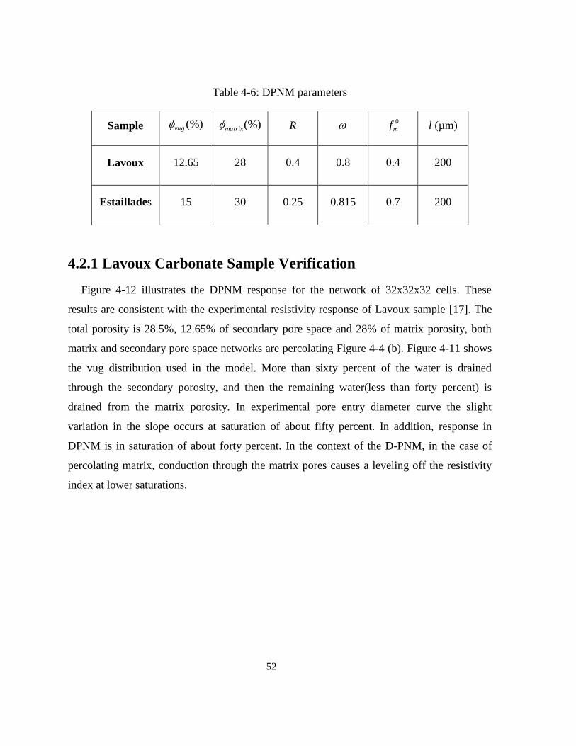
Table 4-6: DPNM parameters ................................................................................................. 52

1

Chapter 1

Introduction

1.1 Carbonate Rocks

1.1.1 Motivation

Statistics demonstrate that the energy consumption has increased significantly in recent

years. Prediction confirms the energy demand could surge by 53%until 2030. Fossil fuels are

the source of more than 85% of world energy consumption. In addition, more than half of the

world’s remaining oil and gas is located in carbonate reservoirs. For example, in the Middle

East, around seventy percent of oil and ninety percent of gas reserves are held in carbonate

reservoirs [1]. Figure 1-1 illustrates the distribution of oil from carbonate reserves around the

world.

Figure 1-1: Distribution of carbonate reservoirs worldwide [1]

2

In the petroleum industry, logging techniques are applied to obtain a continuous record of

the petro-physical properties of reservoir rock by lowering a variety of probes into the

borehole. Interpretation of logging tool measurements determines valuable information about

the existence and volume of hydrocarbon reserves. Figure 1-2showsa sample logging record

combining traces from three different logging tools. The formation resistivity response of the

rock is observed in the second column of Figure 1-2.

Figure 1-2: Example of well logging record [1]

Formation resistivity is of paramount importance for the determination of hydrocarbon

reserves. Consider, for example, the traces shown in Figure 1-2. Whereas other logs

(neutron, density, gamma-ray) can identify lithology (sandstone vs. shale), quantify porosity

and distinguish gas from liquid (oil and brine), it is interpretation of the resistivity log that

enables detection of reservoir zones containing significant amounts of oil. Such

interpretation has been traditionally based on Archie’s laws, which relate the electrical

3

resistivity of reservoir rock to water saturation, wS . These laws, which are obeyed by clean

water-wet sandstones [2] are stated below:

n

wt S

R

RRI

0

(1-1)

m

wR

RF 0 (1-2)

nmwt SRR (1-3)

In the above equations RI is the so-called resistivity index, defined as the ratio of the

resistivity of partially water-saturated rock, tR , to the resistivity of the fully water-saturated

rock, 0R . F is the so-called formation factor, defined as the ratio of the resistivity of the fully

water-saturated rock to the resistivity of a volume of brine of identical dimensions, wR . In

Equation 1-3, which is produced by combining Archie’s laws, is the porosity of the rock,m

is the cementation exponent and n is the saturation exponent.

Non-Archie Behavior of Carbonate Rocks

Archie relations are often employed with the assumption that cementation and saturation

exponents (m and n) would be equal to two, as is typically the case for sandstones and clean

rocks. Carbonate rocks, however, exhibit significant deviations from Archie’s laws; the

cementation and saturation exponent may vary widely from 1.45 to 5.4. Dixon and Marek

(1990) reported that saturation exponent could vary to much less than two (1.3 to 1.8) in

carbonate reservoir [3],while for various types of carbonates cementation exponent value

may range from about 1.5 to 5.4 [4]. Similarly, Saner (1996) measured the cementation factor

of eighty different carbonate rocks with three different methods [5]. After employing error

analysis on the measured data, he concluded that the Archie cementation factor could not be

reliably used to correlate porosity to the resistivity of fully water-saturated carbonate

samples.

4

In carbonates, not only does the cementation exponent, m, deviate from the classical value

of two, but also the dependence of resistivity index on water-saturation demonstrates

nonlinear trend in log-log scale, contrary to expectation (see equation 1-1). Fleury (2002)

presented experimental measurements of non-linear resistivity Index curve for four different

carbonate samples using the Fast Resistivity Index Measurement method [6]. In his study,

various shapes of resistivity index curves have been observed, particularly at lower values of

the water saturation. The saturation exponent varied with saturation from approximately one

to three (see Figure 1-3).

Figure 1-3: Non-Archie behavior of carbonate rocks [6]

In addition, nonlinear behavior of the resistivity index curve has been reported by Padhy et

al.(2006) for six different carbonate samples. Cementation factors in these samples ranged

from 1.99 to 2.68 [7].

The deviations mentioned above are believed to originate from the existence within

carbonate rocks of at least two different pore systems at rather disparate length scales, but

these deviations have not been completely quantified to date. Petricola and Watfa

(1995)considered a dual pore geometry to highlight the significant influence of micro-

porosity on electrical resistivity and the estimation of water saturation thereof [8]. They

suggested that the observed low resistivity behavior may be the result current transport along

a parallel conduction path formed by water-saturated micropores. They concluded that two

5

parameters are essential for the modeling of carbonate rocks with heterogeneous structure:

the amount and the distribution of micro-porosity relative to macroporosity. In their view, the

first step for solving this problem was the measurement of the pore size distribution of

carbonate rocks. They presented a saturation equation to consider the effect of parallel

current-carrying path for two pore size populations (macro and micro).In their equation the

conductivity ( ) is determined by:

)(

n

w

mm

wM

m

MwM SSCCCC M

(1-4)

where wM CCC ,, are the conductivities of vug network, matrix network, and water

respectively. M is the macro intergranular porosity and is the micro-porosity. wS refers to

the saturation while m and n are the cementation factor and saturation exponent respectively

(including subscripts ‘M’ for macro-porosity and ‘ ’ for micro-porosity). It must be noted

that while equation (1-4) can be made to fit certain types of non-Archie behavior after

adjusting the four exponents, it gives no insight on the way the water saturation of the two

different pore populations changes during drainage of the aqueous phase.

Dixon and Marek (1990) studied two different Middle Eastern carbonate samples with

low saturation exponent (median of 1.45) using Scanning Electron Microscopy and high

pressure mercury porosimetry. Two pore size populations (inter-particle macro-pores and

inter-particle micro-pores) were detected in their experimental study of low resistivity

carbonates. They suggested that a network of interconnected micro-pores may be the cause of

anomalously low saturation exponents [3]. However, Dicker and Bemelmans (1984)

observed that the bending down resistivity behavior at low saturation is strongly depended on

thick water layer [9]. This was later confirmed by Han et al. (2007) who reported that the

low resistivity behavior is due to the existence of a thick water film [10].

On the other hand, Sen (1997) has pointed out the anomalously large resistivity increase as

the conducting water phase becomes trapped in isolated regions. He considered three

different pore size distribution (micro-porosity, macro-porosity and vugs) and employed

effective medium theory to compute the effect of micro-porosity on resistivity [11]. He

6

indicated that the dependence of electrical resistivity on water saturation is significantly

modified when the main current-transporting pathway is changed as a result of desaturation.

The effect of secondary porosity on the electrical conductivity of water-saturated carbonates

containing both micro-pores and macro-pores (vugs and solution channels) has been

analyzed by Ioannidis and coworkers (1997) using direct numerical simulation [12]. They

proposed that the cementation exponent in these types of rocks is related to the spatial

connectivity of the secondary pore system in addition to the amount of micro-porosity and

macro-porosity. More recently, attention was drawn to the effect of percolation of secondary

porosity, by Montaron (2009) who interpreted empirically non-Archie resistivity curves

using a water connectivity correction index [13].

As mentioned above, most studies conclude that the non-Archie behavior of carbonate

rocks is attributed to the geology of heterogeneous porous medium and connectivity of the

porosity (percolation). Zou et al. (1997) developed a simple bond model to consider the

effect of wettability on electrical resistivity of porous media by implementing percolation

concepts [14]. They concluded that the simple model is not capable of reproducing the

observed deviation and emphasized the need to take into account the effect of water

remaining in corners and crevices of otherwise drained pores. Padhy et al. (2006) modified

the saturation equation proposed by Pericola and Walfa based on connectivity of two pore

size populations (micro-pores and macro-pores) and included a layer of water in pore

boundaries for a water-wet system [15]. The theoretical resistivity model results compared

favorably to the measured experimental one.

Fleury (2002) proposed a double porosity conductivity model (DPC) and triple porosity

conductivity model (TPC) to explain the nonlinear behavior in carbonate resistivity curves

[6]. The DPC model was employed to reproduce the bending down of RI at low saturations.

In this model, two porosity populations are considered in parallel current-carrying paths. The

TPC model was implemented to explain the bending up at high and intermediate water

saturations and bending down at low saturation. Three different pore size distributions are

imagined in the model (micro-pores, meso-pores and macro-pores). Meso-pores and macro-

pores are assumed to act electrically in series and the sum of them is in parallel with the

7

micro-pores. Both models reproduce the bending down shapes due to the electrical parallel

path. For the other non-linear shapes, he suggested that the parallel conductivity path should

be considered for their modeling.

Han et al. (2007) investigated the effect of continuous thick water films on the electrical

resistivity using numerical computation carried out directly on micro-tomographic images

from four different groups of sandstones and carbonates [10]. These four different textures

are classified based on size, distribution and connectivity of the pores containing both single

pore size distribution and bimodal pore size distribution. The authors demonstrated that, at

low levels of the water saturation, the electrical behavior is dominated by conduction via

continuous water films covering the solid surface, resulting in a significant decrease of the

apparent resistivity exponent. Han et al. further proposed that for carbonate samples with a

double pore size distribution, the electrical behavior depends strongly on the spatial

distribution and connectivity of the micro-porosity [16].

Recently, Bauer et al. (2011) reproduced electrical responses of two different carbonates

(Estaillades and Lavoux carbonates) using a Dual Pore Network Model(D-

PNM)parameterized on the basis of extensive analyses of high-resolution micro-tomographic

data [17].Their work, which to our knowledge represents the most sophisticated attempt in

quantifying the electrical resistivity behavior of carbonates, drew the attention to significant

uncertainty owed to the inability of currently available methods to resolve all length scales of

relevance to current transport.

1.2 Objectives

With the exception of the work of Bauer et al. (2011), the models developed to explain the

non-Archie behavior of carbonate rocks are purely empirical. When these models are fitted

successfully to experimental data, little insight is provided on the relationship between best-

fit parameters and measurable attributes of the microstructure [17]. These models do not

resolve carbonate rock microgeometry to any extent beyond asserting volume fractions and

cementation and saturation exponents for different pore populations. More importantly,

these models make no attempt to quantify the connectivity of different pore populations.

8

While they aid conceptual understanding, they cannot be informed by petrophysical

measurements and are, for this reason, of little predictive value. The work of Bauer et al.

(2011) on the other hand, has advocated detailed pore network extraction directly from

microtomographic data. While x-ray microtomography is common nowadays, pore network

extraction is a difficult task fraught by limitations in the ability of presently available

instruments to resolve all pore length scales in carbonate rocks.

The main hypothesis of this thesis is that there exists a minimal parametrization of a dual

pore network model (D-PNM) that captures most, if not all, features of carbonate rock

microstructure that are essential to the quantitative, sample-specific, modeling of electrical

resistivity. The model is an extends of the original work of Ioannidis (1993) (see also [18])

on the capillary properties of heterogeneous carbonate rocks by endowing the D-PNM with

the capability to the resistivity index under condition of drainage.

We demonstrate that the model is capable of generating the behavior of electrical

resistivity for two different types of carbonates (Estaillades and Lavoux carbonates)

discussed in the recent literature by Bauer et al. (2011) [17] and is consistent with the

capillary pressure data. Parametric studies further confirm the model’s ability to stylistically

reproduce all documented deviations of the resistivity index from Archie behavior [6],

suggesting opportunities for rapid assessment via a constrained optimization approach

conditioned on micro-tomographic data.

9

Chapter 2

Background

2.1 Pore Structure Parameters

2.1.1 Porosity of Reservoir Rocks

Porosity is the percentage of bulk rock volumes occupied by pores that is the fraction of

void space. This pore volume fraction contains the fluids inside the rock and may change

from zero to one. There are two types of porosity. One is porosity which is formed during the

rock deposition process, termed primary porosity and porosity that is the result of post-

depositional and diagenetic process, termed secondary porosity. Different experimental

methods of measuring the porosity d have been reviewed in detail by Dullien [19].

The porosity of sandstone may vary between 10% and 30%. In carbonate rocks the

porosity varies widely due to numerous diagnetic processes which can reduce or increase the

porosity of initial sediments [20].The primary and secondary porosities are related by the

following equation:

m

msv

1 (2-1)

where v is the secondary porosity (vugs), s is the total porosity and m is the primary

porosity (matrix).

2.1.2 Permeability of the Porous Media

Permeability (k) measures the conductivity of the medium to flow and it is only a function

of the geometric and topological characteristics of the porous media. The absolute

permeability is described mathematically by Darcy’s law:

10

gPk

v

(2-2)

where v is the named “filter” velocity vector, P is the pressure gradient, is the fluid

viscosity, is the fluid density and g is the acceleration due to gravity [19].

2.1.3 Capillary Properties

2.1.3.1 Capillary Pressure in Porous media

The existence of surface tension gives rise to a pressure difference across a curved

interface separating two immiscible fluids at equilibrium. At equilibrium, the surface tension

must be balanced out with a pressure differences, which is described mathematically by

Laplace’s equation [21]:

m

wnwR

PP2

(2-3)

where is the surface tension or the interfacial tension, mR is the mean radius of curvature

of the interface and nwP and wP are pressures of non-wetting and wetting phase respectively.

The mean radius of the curvature of each fluid-fluid interface is a function of the local

pore space geometry and the wettability of the solid surface, the latter measured by the

contact angle. For capillaries of simple cross-section, the capillary pressure is generally

described as:

c

wnwr

fPP

)( (2-4)

where, cr is a characteristic pore size and )(f is a function of the contact angle formed

between two immiscible fluids and the pore wall.Capillary Pressure Curves

Interfacial configurations realized during quasistatic immiscible displacement of one fluid

by another in porous media, give rise to a relationship between capillary pressure and wetting

11

phase saturation – the so-called capillary pressure curve. Capillary pressure curves exhibit

hysteresis between drainage (decreasing wetting phase saturation) and imbibition (increasing

wetting phase saturation), as shown in Figure 2-1.

Figure 2-1: Mercury capillary pressure curve

2.1.3.2 Break through Capillary Pressure

During the drainage of a wetting phase by a non-wetting one, a characteristic value of

capillary pressure (the breakthrough capillary pressure) is associated with the first formation

of a sample-spanning (percolating) connected pathway of pores invaded by the non-wetting

phase.0The breakthrough pressure can be identified with the inflection point in the drainage

capillary pressure curve.Since the connected pathway associated with breakthrough of the

non-wetting phase comprises the largest pores, it is not surprising that the breakthrough

capillary pressure is strongly correlated with permeability. Such a correlation has been

reported by Chatzis (1980) for sandstones [22]:

369.063.85 kPc (2-5)

where

cP is the mercury-air capillary pressure in psi and is the absolute permeability in

mDarcy.

12

Non-wetting phase breakthrough in a network of pores happens as the non-wetting phase

invades a number of interconnected pores. The breakthrough capillary pressure or

penetration of a non-wetting phase (e.g., air) into a pore throat of rectangular cross-section

may be computed by implementing the following approach, originally put forward by

[23]for pores of square cross-section, and later extended by Ioannidis (1993) derived the

following expression relating the dimensionless capillary pressure as a function of the

dimentionless interface radius of curvature [20]:

)(

)(cos)1(

2

2'

1

''

R

RRc

FR

FRP

(2-6)

where,

)4

sin(cos22)22

()(1 RRRRF

(2-7)

)4

()4

(sin)22

sin(2

1)( 2

2 RRRRF

(2-8)

bPP c

c ' (2-9)

b

RR '

(2-10)

where'

cP and 'R are dimensionless capillary pressure and dimensionless radius. cP is the

capillary pressure, b is the side length of the throat, is the interfacial tension and R is the

interface radius of curvature. The breakthrough capillary pressure that may be realized inside

pore throats is the minimum capillary pressure of the interface. Therefore, it is determined by

computing the minimum'

cP by employing:

0'

'

dR

dPc (2-11)

By differentiating from equation (2.5), we obtain:

13

0)()(cos)1(2)()( 1

'

221

2' RRRRR FRFFFR (2-12)

After calculating the roots of equation (2-12), the non-negative root 'R is substituted in

equation (2-5) to determine'

cP .The breakthrough capillary pressure of the throat is then

obtained from equation (2-8).

2.1.4 Electrical Properties

The porous media contain solid grains and void spaces which may occupy by fluids. In

petroleum reservoirs, mainly the solid and hydrocarbon phases (gas and oil) are non-

conductive. The conducting phase of the rock is the water including dissolved salts.

Therefore, the electrical properties of the rock depend on the saturation of the conducting

fluid and its distribution inside the voids [24].

14

Chapter 3

Dual Pore Network Model

3.1 Model Development

3.1.1 Geometry of the Dual Pore Network Model

The dual pore network model (DPNM) corresponds to a tessellation of the bulk rock space

in cubic cells of side length . The model is an attempt to provide a minimalist description of

carbonate pore space by capitalizing on local porosity information that is nowadays readily

available by x-ray microtomography. Such information consists of 3D maps of local porosity,

s , which may be further differentiated into matrix porosity that is typically below the

resolution limit, and resolved secondary or vuggy porosity [17]. Accordingly, each cell

comprises a cubic vug (of side length a) connected to six channels with rectangular cross-

sections (of side length b, where R = b/a). Consider a cubic cell of bulk volume3l identified

by its spatial location (x, y, z), as shown in Figure 3-1. The cell contains a vug body of side

length a(x,y,z). Connection to vugs in adjacent cells is provided by six throats of side length

b(x,y,z) )),,(),,(0( zyxazyxb drilled into each face of the cubic cell towards the central

vug. The remainder of the cell volume is occupied by rock matrix of unresolved geometry.

The vuggy porosity (fraction of the cell bulk volume occupied by secondary pores), v ,is

expressed in terms of the side length of the vug body, a(x,y,z), the size of the cubic celll, and

the aspect ratio R as shown below [18].

2

3

3

2 ),,(3

),,()31(),,(

l

zyxaR

l

zyxaRzyxv (3-1)

where,

lzyxa ),,(0

15

10 R

Given v , R and l, a(x,y,z)is determined by solving equation (3-1)and b(x,y,z)is computed as

R, a(x,y,z).

Figure 3-1: A cubic cell as the basic building block of a dual pore network model.

3.1.2 Assignment of Cell Properties

As mentioned before, each cell comprises geometrically unresolved porosity (hereafter

referred to as matrix) characterized in terms of macroscopic properties (porosity,

permeability, capillary pressure, cementation and saturation exponents) which are assumed to

be known. Matrix properties may be spatially distributed and/or cross-correlated.

Additionally, geometrically resolved secondary porosity in the form of a cubic vug and

connecting throats is also present. Ideally, ),,( zyxv is known from 3D microtomographic

images. In the absence of such information we assume here that the secondary porosity is a

random variable following the Weibull distribution with no spatial correlations. The

probability density function of Weibull-distributed random variable x is given by

16

00

0)(),,(

)(1

x

xexk

kxf

kxk

(3-2)

where k and are the shape parameter and scale parameter, respectively. The mean of the

distribution is calculated as

)1

1(k

Mean (3-3)

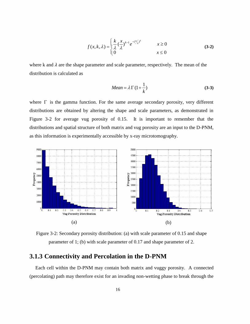
where is the gamma function. For the same average secondary porosity, very different

distributions are obtained by altering the shape and scale parameters, as demonstrated in

Figure 3-2 for average vug porosity of 0.15. It is important to remember that the

distributions and spatial structure of both matrix and vug porosity are an input to the D-PNM,

as this information is experimentally accessible by x-ray microtomography.

(a)

(b)

Figure 3-2: Secondary porosity distribution: (a) with scale parameter of 0.15 and shape

parameter of 1; (b) with scale parameter of 0.17 and shape parameter of 2.

3.1.3 Connectivity and Percolation in the D-PNM

Each cell within the D-PNM may contain both matrix and vuggy porosity. A connected

(percolating) path may therefore exist for an invading non-wetting phase to break through the

17

entire pore network via matrix pores, secondary pores (vugs) or a combination of both. The

degree of percolation of both matrix and vuggy porosity can be adjusted independently in the

DPNM. The percolation of the matrix pore space is modified by designating a fraction 0

mf of

cells to have negligible matrix porosity. Cells with non-zero matrix porosity are assigned a

uniform value of matrix porosity, m , such that the average matrix porosity of the entire D-

PNM is m

o

mf )1( In the absence of spatial correlations, 32.0)1( o

mf ensures percolation

of the matrix in 3D (Ioannidis et al, 1993). Figure 3-3 represents a schematic of two-

dimensional networks of 10x10 cells in which either one or both matrices and secondary

porosities form percolating networks. A D-PNM in which the matrix percolates is shown in

Figure 3-3(a) whereas, Figure 3-3(b) illustrates a D-PNM with non-percolating matrix.

Furthermore, the connectivity of the secondary pore space (vugs) may be adjusted to

obtain models with varying degrees of percolation of an invading non-wetting phase via

secondary pore space. Since each cell containing a cubic vug is also assumed to contain six

throats providing communication to secondary pore space in neighboring cells, vug

connectivity is adjusted using a probabilistic rule that takes account the amount of vug

porosity in adjacent cells. The strength of the probability for a communication to exist

between two adjacent cells is controlled by a connectivity exponent (taking values

between zero and one). For two neighboring blocks located at point x and*x , the probability

of finding connection between them ( ),( *xxp

) is proportional to the product of local vug

porosity values and it can be expressed by equation (3-4) [18]. Figure 3-3(a) and Figure 3-

3(c) demonstrate the case where 9.0 and 2.0 , leading to the percolating and non-

percolating secondary porosity respectively.

1

** )](.)([),( xxxxp vv

(3-4)

where,

10

18

1),(1)(1)(

0),(0)(0)(**

**

xxpxandxif

xxpxorxif

vv

vv

matrix porosity

solid secondary porosity

(a)

(b)

(c)

Figure 3-3:Cartoon representation of DPNM with 10x10 cells: (a) Percolating vugs in

percolating matrix; (b) Percolating vugs in non-percolating matrix; (c) Non-percolating vugs

in percolating matrix.

3.2 Computation of Drainage Capillary Pressure Curve

3.2.1 Cell Accessibility to Invading Non-wetting Phase

In DPNM, each cell may be invaded by a non-wetting phase via matrix or secondary pores

according to the rules governing capillarity-dominated displacement. A cluster multiple

labeling algorithm is employed to determine the fluid occupancy of matrix and secondary

porosity in each cell. This enables the determination of water saturation as a function of

increasing capillary pressure.

19

3.2.1.1 Identification of “Open” cells

The first step in the modeling of capillary pressure versus saturation relationship using the

D-PNM is the identification of cells with the potential to be invaded by the invading non-

wetting phase, hereafter referred to as “open” cells, at each level of applied capillary

pressure. In general, each cell may be penetrated through matrix pore space or vuggy

porosity. Penetration of the non-wetting phase into the matrix is limited by the matrix

breakthrough capillary pressure, whereas penetration into the secondary pore space is limited

by a breakthrough capillary pressure dependent on the size of vug throats. . The calculation

of breakthrough capillary pressure of the matrix is explained in section 2.1.3.2. Using the

dimensions of cubic vug and connecting throats the breakthrough capillary pressure of the

vugs is obtained for each cell as discussed in section 2.1.3.2. The smaller of the two is the

capillary pressure at which non-wetting phase first enters the cell (cell breakthrough

pressure) as the externally applied capillary pressure is increased in a step-wise fashion.

Specifically, at each level of externally applied capillary pressure a cell is marked as “open”

if the cell breakthrough pressure is smaller than the externally applied capillary pressure, in

the computer program, an array stores binary indicator values where 1 identifies open cells.

3.2.1.2 Clustering of Open Cells

In order to follow the invasion of cells within the D-PNM by a non-wetting phase it is

necessary to determine the accessibility of open cells at each level of externally applied

capillary pressure. This is so because cells which are open at any given value of capillary

pressure may not be part of a cluster of adjacent open cells with a connection to the invasion

boundary surface. Clustering of open cells is achieved by an algorithm originally due to

Hoshen and Kopelman [25]after some modifications as explained next.

The original 2-dimensional Hoshen-Kopelman algorithm assigns unique labels to distinct

clusters of occupied or unoccupied cells on a grid. Figure 3-4 demonstrates the cluster

labeling for an occupied (indicator value of one) cells in a hypothetical matrix. Assuming 4-

neighbor adjacency, the presence of five different clusters is detected by the HK algorithm.

Cells belonging to the same cluster share the same cluster label.

20

1 1 1 1 0 0 0 0

1 1 1 1 0 0 0 0

0 1 1 0 1 0 1 1 0 1 1 0 2 0 3 3

0 0 0 1 1 1 0 1 0 0 0 2 2 2 0 3

0 0 0 1 1 1 0 0 0 0 0 2 2 2 0 0

1 1 1 1 1 0 0 0 2 2 2 2 2 0 0 0

0 1 1 0 0 0 1 0 0 2 2 0 0 0 4 0

0 0 1 0 0 1 1 1 0 0 2 0 0 4 4 4

1 1 0 0 0 1 1 0 5 5 0 0 0 4 4 0

Figure 3-4: Hoshen-Kopelman Cluster multiple labeling technique.

The basic 2-D HK algorithm has two data structures serving the following functions [26].

1. The working matrix

Stores occupied (indicator value of one) and unoccupied (indicator value of zero)

cells.

2. Cluster label Array (Csize)

Counts the cluster labels.

Can have positive or negative value.

Figure 3-5 illustrates the HK matrix and Csize array data structures

Matrix Csize

1 1 1 1 0 0 0 0 1

2

3

4

5

6

7

0

0 1 1 0 1 0 1 1 0

0 0 0 1 1 1 0 1 0

0 0 0 1 1 1 0 0 0

1 1 1 1 1 0 0 0 0

0 1 1 0 0 0 1 0 0

0 0 1 0 0 1 1 1 0

1 1 0 0 0 1 1 0

Figure 3-5: Hoshen-Kopelman data structure

21

Matrix Procedure: The matrix is traversed row-wise to identify members of same cluster by

checking its four neighbors as demonstrated in Figure 3-6. Each cell’s attribute (“open” or

not) is checked and if the cell is “open”, it is assigned the same cluster label as the neighbor’s

label. The Csize array is changed as will be described below). If no neighbor from which to

inherit a cluster label is found, then a new cluster label is assigned to the cell. Figure 3-7is a

flow chart of the matrix traversing procedure [25].

i-1 , j

i , j-1 i , j i , j+1

i+1 , j

Figure 3-6: HK cell neighboring cells

22

Figure 3-7: Flow chart of classical HK algorithm

Csize Array Procedure:

Csize contains two types of values:

Positive value: number of members associated with this cluster label.

Negative value: label redirection. All of the clusters with negative value belong to

the other clusters.

Figure 3-8 explains the purpose and function of the Csize array for 2-D clustering. As shown

in Figure 3-8(a), cluster 1 has 6 members. Figure 3-8(b-d) has the same pattern to fill the

cluster number. Cluster 4 has the same value as 2 in Figure 3-8(e). The same procedure is

followed for other clusters. After all the occupied cells are labeled, the Csize array will be

scanned again to fix any negative values. In Figure 3-8 (h) the Csize values associated with

cluster labels 4 and 5 are -2. This indicates that all cells given the label 4 (and 5) belong to

cluster number 2.All cells with the value of 7 belong to cell number 6. The final clustered

matrix is demonstrated in Figure 3-8(i).

Label the proper cluster size

from the Csize array to the

neighboring cells

Go to next

cell

Is the cell

occupied

Any of the

neighbors

occupied?

Assign new label

to the cell

No

No Yes

Yes

23

Matrix Csize

1 1 1 1 0 0 0 0 1

2

3

4

5

6

7

6

0 1 1 0 1 0 1 1 0

0 0 0 1 1 1 0 1 0

0 0 0 1 1 1 0 0 0

1 1 1 1 1 0 0 0 0

0 1 1 0 0 0 1 0 0

0 0 1 0 0 1 1 1 0

1 1 0 0 0 1 1 0

(a)

Matrix Csize

1 1 1 1 0 0 0 0 1

2

3

4

5

6

7

6

0 1 1 0 2 0 3 3 1

0 0 0 1 1 1 0 1 2

0 0 0 1 1 1 0 0 0

1 1 1 1 1 0 0 0 0

0 1 1 0 0 0 1 0 0

0 0 1 0 0 1 1 1 0

1 1 0 0 0 1 1 0

(b)

Matrix Csize

1 1 1 1 0 0 0 0 1

2

3

4

5

6

7

6

0 1 1 0 2 0 3 3 1

0 0 0 1 1 1 0 1 2

0 0 0 1 1 1 0 0 0

1 1 1 1 1 0 0 0 0

0 1 1 0 0 0 1 0 0

0 0 1 0 0 1 1 1 0

1 1 0 0 0 1 1 0

(c)

24

Matrix Csize

1 1 1 1 0 0 0 0 1

2

3

4

5

6

7

6

0 1 1 0 2 0 3 3 1

0 0 0 4 1 1 0 1 2

0 0 0 1 1 1 0 0 1

1 1 1 1 1 0 0 0 0

0 1 1 0 0 0 1 0 0

0 0 1 0 0 1 1 1 0

1 1 0 0 0 1 1 0

(d)

Matrix Csize

1 1 1 1 0 0 0 0 1

2

3

4

5

6

7

6

0 1 1 0 2 0 3 3 3

0 0 0 4 2 1 0 1 2

0 0 0 1 1 1 0 0 -2

1 1 1 1 1 0 0 0 0

0 1 1 0 0 0 1 0 0

0 0 1 0 0 1 1 1 0

1 1 0 0 0 1 1 0

(e)

Matrix Csize

1 1 1 1 0 0 0 0 1

2

3

4

5

6

7

8

6

0 1 1 0 2 0 3 3 7

0 0 0 4 2 2 0 3 3

0 0 0 2 2 2 0 0 -2

1 1 1 1 1 0 0 0 0

0 1 1 0 0 0 1 0 0

0 0 1 0 0 1 1 1 0

1 1 0 0 0 1 1 0

(f)

25

Matrix Csize

1 1 1 1 0 0 0 0 1

2

3

4

5

6

7

8

6

0 1 1 0 2 0 3 3 12

0 0 0 4 2 2 0 3 3

0 0 0 2 2 2 0 0 -2

5 5 5 2 2 0 0 0 -2

0 1 1 0 0 0 1 0 0

0 0 1 0 0 1 1 1 0

1 1 0 0 0 1 1 0

(g)

Matrix Csize

1 1 1 1 0 0 0 0 1

2

3

4

5

6

7

8

6

0 1 1 0 2 0 3 3 15

0 0 0 4 2 2 0 3 3

0 0 0 2 2 2 0 0 -2

5 5 5 2 2 0 0 0 -2

0 5 5 0 0 0 6 0 6

0 0 5 0 0 7 6 6 -6

8 8 0 0 0 7 6 0 2

(h)

Matrix Csize

1 1 1 1 0 0 0 0 1

2

3

4

5

6

7

8

6

0 1 1 0 2 0 3 3 15

0 0 0 2 2 2 0 3 3

0 0 0 2 2 2 0 0 6

2 2 2 2 2 0 0 0 2

0 2 2 0 0 0 4 0 0

0 0 2 0 0 4 4 4 0

5 5 0 0 0 4 4 0 0

(i)

Figure 3-8: Csize procedure in HK algorithm

26

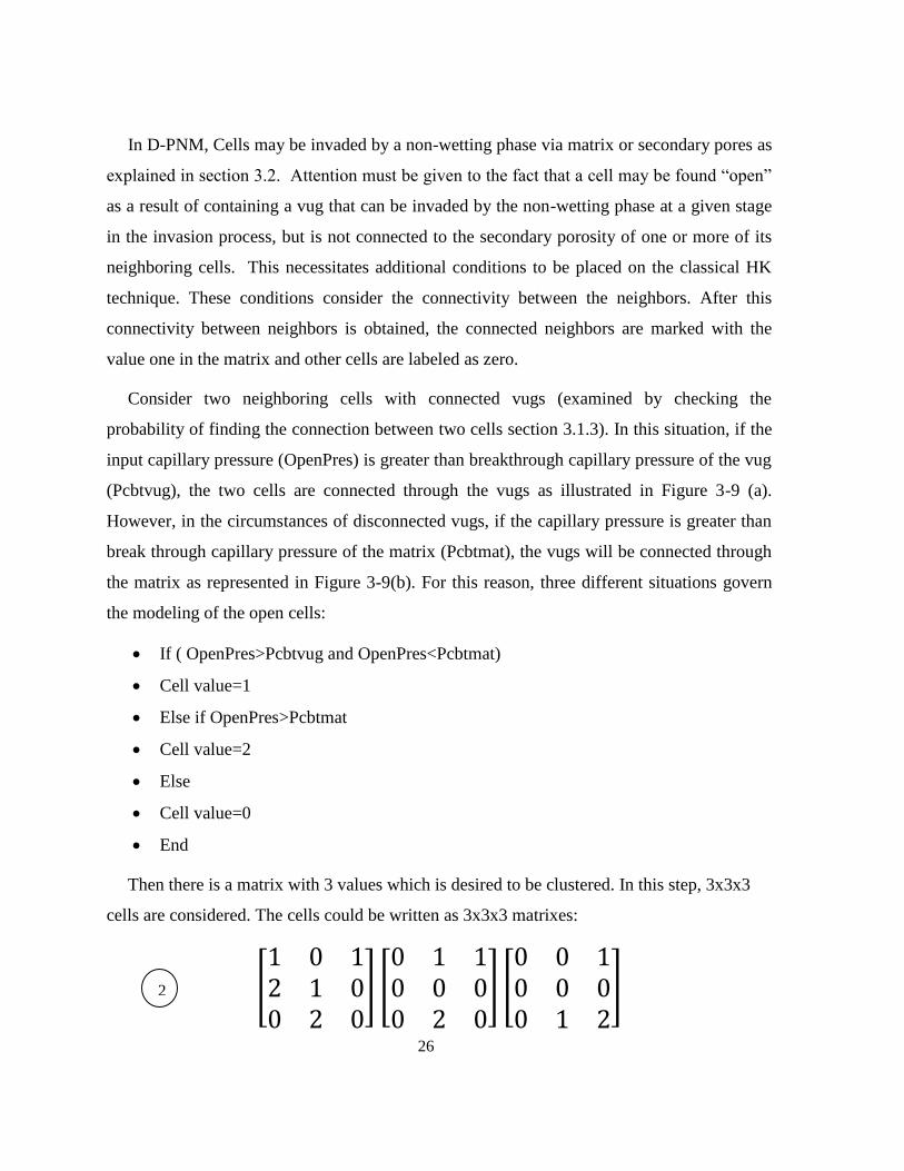
In D-PNM, Cells may be invaded by a non-wetting phase via matrix or secondary pores as

explained in section 3.2. Attention must be given to the fact that a cell may be found “open”

as a result of containing a vug that can be invaded by the non-wetting phase at a given stage

in the invasion process, but is not connected to the secondary porosity of one or more of its

neighboring cells. This necessitates additional conditions to be placed on the classical HK

technique. These conditions consider the connectivity between the neighbors. After this

connectivity between neighbors is obtained, the connected neighbors are marked with the

value one in the matrix and other cells are labeled as zero.

Consider two neighboring cells with connected vugs (examined by checking the

probability of finding the connection between two cells section 3.1.3). In this situation, if the

input capillary pressure (OpenPres) is greater than breakthrough capillary pressure of the vug

(Pcbtvug), the two cells are connected through the vugs as illustrated in Figure 3-9 (a).

However, in the circumstances of disconnected vugs, if the capillary pressure is greater than

break through capillary pressure of the matrix (Pcbtmat), the vugs will be connected through

the matrix as represented in Figure 3-9(b). For this reason, three different situations govern

the modeling of the open cells:

If ( OpenPres>Pcbtvug and OpenPres<Pcbtmat)

Cell value=1

Else if OpenPres>Pcbtmat

Cell value=2

Else

Cell value=0

End

Then there is a matrix with 3 values which is desired to be clustered. In this step, 3x3x3

cells are considered. The cells could be written as 3x3x3 matrixes:

[

] [

] [

] 2

27

a bL

(a)

a bL

(b)

Figure 3-9: Connectivity between neighboring cells

Each cell has three neighbors located on the left, under and inside, in three different

dimensions as displayed in Figure 3-10.Two neighboring cells may be open or not open

(indicated as one or zero). They also may be connected or disconnected (one or zero). The

model will assign two neighbors in the same cluster only if the multiplication of these two

conditions, open and connected, equals one. Similar procedure to the classical HK for

checking the matrix and Csize would be used after this point.

28

(i,j,

k-1)

(i,j-1,k) (i,j,k)

(i-1,j,k)

Figure 3-10: nearest three neighbors

3.2.1.3 Accessible Clusters

After determining the open clusters, cells belonging to the clusters that are linked to the

inlet face of the network are considered as accessible clusters. To obtain accessible cells,

initially, the surface which is employed to drain the wetting phase from the network (either

one of x, y or z) is chosen. The code is programmed to distinguish the clusters connected to

the inlet face and make the other ones zero. The work flow is represented in Figure 3-11.

29

Figure 3-11: Work flow of the model to find the accessible cluster through the inlet surface

3.2.2 Fluid Saturation Calculations

Determination of the water saturation of the D-PNM for each capillary pressure step is

explained in this section. This is done in two stages. Initially saturation of each accessible

cell’s is estimated. Then, the total saturation of the DPNM is computed as the weighted

average of individual cell saturation values.

3.2.2.1 Saturation of Each Open Cell

The non-wetting phase saturation in each accessible cell is calculated as the following

average [20]:

Start

Calculate side length

of pore bodies and

throats,total porosity

of the network,

connectivity between

cells

For each penetration

step: capillary

pressure is greater than breakthrough

capillary pressure of the cell

Cell is

closed to

NWP

Cell is open

to NWP

No

Cluster open cells by

using Hoshen-

Kopelman algorithm

Calculate the

saturation of

accessible cells

End

Yes

Choose the

inlet face

Obtaining

accessible clusters

trough the inlet

surface

Calculate the

electrical resistivity All cells

checked

No Yes

30

s

mnwmvvnwvnw

SSS

1 (3-5)

where v is the vuggy porosity, vnwS is the non-wetting phase saturation in the secondary pore

space , m is the matrix porosity, is the non-wetting phase saturation in the matrix, and

s is the overall cell porosity. v is obtained from the invers Weibull distribution for each

cell and m is assumed to be uniform for all cells in network as is explained in section 3.1.2.

To calculate s , the following equation is employed [20]:

m

msv

1 (3-6)

The next two sections explain precisely how to obtain vnwS and mnwS .

3.2.2.2 Vug Saturation

Due to the angular cross-sectional shape of the vug bodies and throats in the D-PNM, the

wetting phase is not displaced completely by the non-wetting phase upon invasion of the

secondary pores. Rather, the corners of vug pore throats and bodies retain some amount of

wetting phase when they are first invaded. This so-called “corner” saturation decreases

further as the capillary pressure is increased [23].

For each capillary pressure step, the volume at each corner of the pore throats and pore

body, that is not filled with the non-wetting phase, is determined using the following

approximate equation [27]:

)())2

(( 2

2'

Rcoco FlRbV (3-7)

where coV is volume of unfilled corners, col is the length of the corner, and b is the size length

of the throats (it could be the length of the vug body(a)for the vug body volume). )(2 RF is

31

obtained from equation (2.7) and 'R , the dimensionless radius of curvature of the interface, is

determined by the Laplace equation:

'

' 1

RPc (3-8)

where'

cP is the dimensionless capillary pressure that is calculated for each penetration step

by equation (2.9).

The wetting phase volume remaining within the secondary pore space in each cell after

this space has been invaded by the non-wetting phase is determined by the following

equation:

throats

co

vugbody

co

vug

co VVV (3-9)

Each cell has one cubic pore body and six pore throats. Each pore body has eight corners and

the total volume of unfilled corners for vug body is determined from equation (3-

10).Moreover, each throat has four corners (total of twenty four corners in each cell) and

throats

coV is calculated by equation (3-11), where the function F2 is defined by equation (2-7).

)())2

((8 2

2'

R

vugbody

co FaRaV (3-10)

)(2

)1())

2((24 2

2'

R

throats

co Fa

RbV

(3-11)

)())2

((8)(2

)1())

2((24 2

2'

2

2'

RR

vug

co FaRaFa

RbV

(3-12)

Therefore, the total volume of the vug (vugV ) is equal to:

vugbodythroatsvug VVV (3-13)

32

2

)1(6 a

lbV vug

(3-14)

The above equations are employed to calculate the vug saturation by:

32

)(

)(1

vugV

vugVS co

vnw

(3-15)

3.2.2.3 Matrix Saturation

To identify the non-wetting phase saturation of the matrix, the wetting phase saturation is

obtained from a Brooks-Corey model of matrix capillary pressure [20]:

weffc SP* (3-16)

where weffS is effective wetting phase saturation of matrix. *

cP is the reduced capillary pressure

and is calculated from:

c

cc

P

PP*

(3-17)

where

cP is the breakthrough capillary pressure of the matrix.

The parameter in equation (3-16) may be estimated from experimental mercury

porosimetry data and weffS is obtained by:

*

cweff PS (3-18)

wr

wrwweff

S

SSS

1 (3-19)

where wS is the wetting phase saturation of the matrix and wrS is a residual wetting phase

saturation. Both and wrS are treated as adjustable parameters in the D-PNM. By

substituting the input capillary pressure and breakthrough capillary pressure in equation (3-

17),*

cP is determined. By substituting achieved *

cP value in equation (3-17) weffS is obtained.

Adopting the estimated weffS and wS is computed with equation (3-18).

33

3.2.2.4 Total Saturation for Accessible Cells

The non-wetting phase saturation of the DPNM for each capillary pressure step is

obtained as the following weighted average equation:

cellsall

cellsall

nw

nwzyx

zyxzyxS

S),,(

),,(),,(

(3-20)

In D-PNM only the accessible cells are non-zero, therefore the saturation of accessible cells

is multiplied by their porosity and added together. The value is then divided by total porosity

of the model to obtain the total saturation for the network.

3.3 Computation of Resistivity Index

3.3.1 Resistivity of a Single Cell

The electrical resistivity of each cell is isotropic and is determined by the assumption that

conduction through matrix is in parallel with conduction through secondary pores, as

explained in equation (3-21), equation (3-22) and Figure 3-12(a - b) presented below.

a b

L/2

Matrix1

Matrix2

Matrix3

Matrix4

VugThroat

(a)

34

(b)

Figure 3-12: (a) Half-cell resistivity along one direction considering; (b) conduction through

matrix in parallel with conduction through secondary pores.

)(||2 vugthroatmatrixL RRRR (3-21)

)(111

2 vugthroatmatrixL RRRR (3-22)

All of matrixR , throatR and vugR are functions of water saturation. To determine matrixR Archie’s

law, with identified m and n (described in section 1.1.1), is implemented.

nm

wt SRR

where tR is the saturated matrix resistivity, wR resistivity of a volume of brine of identical

dimensions, is porosity of the rock and S is the rock saturation. 1matrixR and 2matrixR are equal

to 3matrixR and 4matrixR respectively.

The half-cell resistances throatR and vugR are computed by

A

lR (3-23)

where is the electrical resistivity, l is the length of the conductor and A is the cross sectional

area of the conductor. Similarly for throatR and vugR half-cell) we have:

35

throat

throatA

aLR

2

(3-24)

vug

vugA

aR

2 (3-25)

where throatA and vugA are cross-sectional areas occupied by the conducting aqueous phase.

Prior to drainage of the wetting phase from the secondary pore space in a cell, the value of

and are calculated from the following equations:

22b

aLRthroat

(3-26)

22 a

aRvug (3-27)

As the wetting phase is further drained from the vugs with increasing capillary pressure,

the cross sectional areas throatA and vugA decrease according to the equations (3-28) and (3-29).

The computation of these areas for each capillary pressure is based on the radius of curvature

of the interfaces residing in the corners, which change with capillary pressure according to

equation (3-8). Equations (3-28) and (3-29) explain the effect of radius change on the cross

sectional area of the vug bodies and throats.

2

2'2 FbRAthroat (3-28)

2

2'2 FaRAvug (3-29)

The resistivity of each cell within the D-PNM is modeled by two half-cells in orthogonal

directions. It is assumed that three orthogonal plates will divide one cell, which results in six

resistors as represented in Figure 3-13[28].

36

L/2

Figure 3-13: Single cell represented in 3D by six identical resistors.

The electrical resistivity of the entire D-PNM is determined by a renormalization

approach [29]. Initially eight cells neighboring each other as demonstrated in Figure 3-14(a)

are assumed. All of the resistors in eight cells are considered to be in one electrical circuit.

Figure 3-15(b) displays electrical schematic of the circuit. Assuming a potential difference of

one volt between the beginning and the end point of this circuit, the equivalent resistivity is

calculated by Kirchoff’s equations for the circuit.

(a)

37

(b)

Figure 3-14: Calculation of equivalent resistivity of eight neighboring cells

Same approach is employed for the total network as illustrated is Figure 3-15. First, the

total network is divided in to the groups of eight cells (2x2x2), and then the equivalent

resistor is calculated for each group of 2x2x2 cells implementing the above mentioned

approach. In this process, by replacing eight resistors with 1 equivalent resistor, the number

of cells is decreased into 1/8 of previous amount. This procedure will be continued until

reducing the number of resistors in to one resistor which is the equivalent resistivity of the

total network ( tR ).

Figure 3-15: Schematic of renormalizing 4x4x4 cells to one cell

38

For each penetration step, the resistivity index of the D-PNM ( RI ) is the specified

computed resistivity ( tR ) at any saturation over the resistivity of the fully water-saturated

rock ( 0R ) (equation (1-3)). 0R is the resistivity of the rock at the initial moment(before

desaturation state starts).

0

tRRI

R (1-3)

3.4 Computation of Formation Factor

For calculating the formation factor of the D-PNM, Archie’s law is employed as described

in section 1.1.1.

0

w

RF

R (1-2)

where 0R is the resistivity of the fully water-saturated rockand wR is the resistivity of the

volume of brine of identical dimensions.Calculation of 0R was explained in the previous

section. We compute wR from (equation (3-23)) by substituting the geometry of the system

for length and cross sectional area as follows:

)()(

)(

klil

jlRw

(3-30)

where j is the number of cells along the direction of transport, i and k are the number of cells

in two other directions and l is the side length of each cell.

39

Chapter 4

Results and Discussion

4.1 Model Response

4.1.1 Single Cell Response

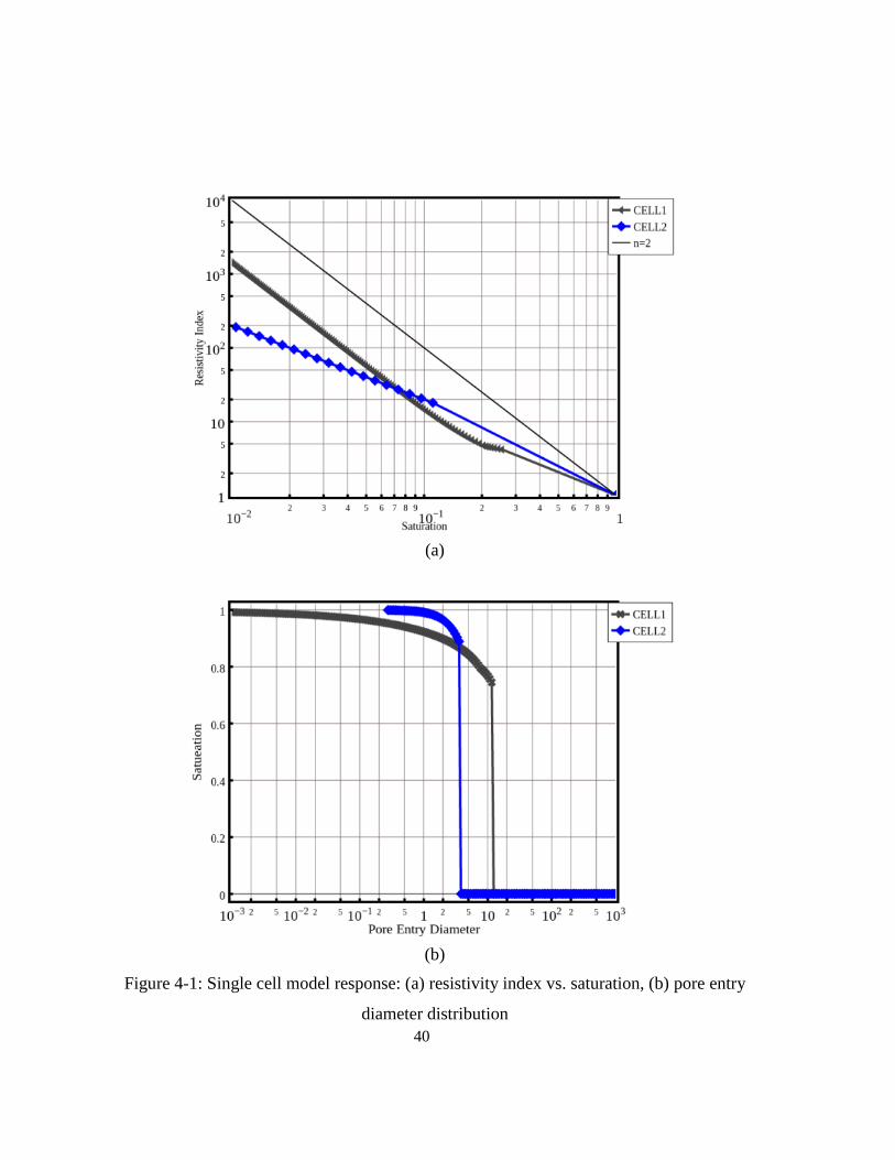
The electrical response of a single cell for two sets of parameters, referred to as CELL1

and CELL2, are presented in Figure 4-1. As it indicated in Table 4-1, both cells contain the

same amount porosity, 2.0s . However, the matrix porosities in the two cells are

different; 05.0m for CELL1 and 0m for CELL2. Furthermore, 1.0R for CELL1

and 03.0R for CELL2. The secondary porosity in CELL1 is invaded when wS is between

0.2 and 0.3. The small plateau until wS = 0.2 is the effect of remaining water in the corners

of the vug. At water saturation of about 0.2 the primary porosity (matrix porosity) is invaded

and RI exhibits a slope of -2, as expected since Archie behavior with n = 2 is assumed for the

matrix. The secondary pore space in CELL2 (with no matrix porosity) is invaded at a higher

capillary pressure as expected given the smaller value of R, corresponding to wS ~ 0.1.

Remaining water in the corners of the secondary pore space is the reason of bending down in

the CELL2 resistivity curve. Remarkably, non-Archie behavior is already exhibited by a

single cell in the D-PNM, attesting to the importance of accounting for porosity at two

different scales.

Table 4-1: Single cell parameters

(%)total (%)matrix R

CELL1 20 0.05 0.1

CELL2 20 0 0.03

40

(a)

(b)

Figure 4-1: Single cell model response: (a) resistivity index vs. saturation, (b) pore entry

diameter distribution

41

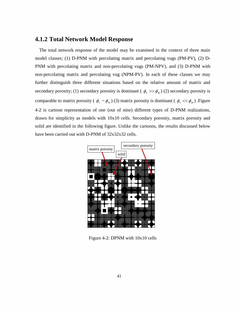
4.1.2 Total Network Model Response

The total network response of the model may be examined in the context of three main

model classes; (1) D-PNM with percolating matrix and percolating vugs (PM-PV), (2) D-

PNM with percolating matrix and non-percolating vugs (PM-NPV), and (3) D-PNM with

non-percolating matrix and percolating vug (NPM-PV). In each of these classes we may

further distinguish three different situations based on the relative amount of matrix and

secondary porosity; (1) secondary porosity is dominant ( mv ) (2) secondary porosity is

comparable to matrix porosity ( mv ~ ) (3) matrix porosity is dominant ( mv ) .Figure

4-2 is cartoon representation of one (out of nine) different types of D-PNM realizations,

drawn for simplicity as models with 10x10 cells. Secondary porosity, matrix porosity and

solid are identified in the following figure. Unlike the cartoons, the results discussed below

have been carried out with D-PNM of 32x32x32 cells.

matrix porosity

solid

secondary porosity

Figure 4-2: DPNM with 10x10 cells

42

Figure 4-3 shows the behavior of the model with only matrix porosity in case of no

secondary porosity. Matrix properties are assumed to be uniform in the simulations

presented in this thesis.

Figure 4-3: Electrical resistivity and capillary pressure properties of the matrix.

4.1.2.1 Percolating Matrix and Percolating Vugs

Figure 4-4 (a), (b) and (c) represent the first class (PM-PV). The responses of the DPNM

for this type of pore structure are illustrated in Figure 4-5. The model parameters for these

results can be seen in Table 4-2. Figure 4-5(a) shows the response of the first D-PNM

member in this class, in which the secondary porosity is significantly higher than the matrix

porosity )07.0~(v

m

, for two different values of R. In the RI curve, more than ninety percent

of the water is drained from the vugs and almost ten percent from the matrix, because of the

significantly higher secondary porosity. Drainage from point (a) to point (b) corresponds

with desaturation of the secondary pore space, for which the dependence of resistivity on

saturation is weaker than predicted by Archie’s law (slope less than -2 on a log-log plot).

When most of the vugs have been invaded by the non-wetting phase, at point (c), resistivity

increases sharply within a short range of water saturation and until the matrix porosity is first

invaded by the non-wetting phase. The sharp increase of resistivity at point (c) is due to the

43

fact that water in the corners of invaded vugs makes a significant contribution to electrical

conductivity – a contribution that depends strongly on water saturation. That is to say, small

changes in the total water saturation (due to loss of water from the corners of drained vugs)

results in a significant increase of electrical resistivity.

Turning now to the capillary pressure vs. water saturation curve, a smaller value of R shifts

the capillary pressure curve to the right. This is expected because for a smaller value of R

(recall that R=b/a) the throats connecting vugs are smaller and, for this reason, the

breakthrough capillary pressure of the vugs is higher. In Figure 4-4(a), the green line

representing RI for the D-PNM with smaller R is shifted downward, indicating a weakening

of the dependence of resistivity on water saturation. This makes sense because the vug

throats are current-carrying paths. Drainage of water from the secondary pore space

corresponds to loss of less significant conductors in the D-PNM with lower R. Similarly, the

effect of loss of water from the corners of drained vugs is diminished in the D-PNM with

lower R.

Figure 4-5(b) shows the response of the second D-PNM member in this class, in which the

secondary porosity is comparable to the matrix porosity )1~(v

m

, for the same two values of

R. About sixty percent of the water is drained from the vugs and forty percent is drained

from the matrix. The behavior of the RI curve observed in Figure 4-5(a) is barely evident

here because the significant amount of matrix porosity results in significant conduction

through the matrix over a broad range of water saturation. A decrease in the value of R

causes a “break” in the RI curve and a reduction of the sensitivity of resistivity on saturation.

Again, this is understood because drainage of water from the secondary pores is results in

loss of less significant conductors (smaller throats). At point (d), the slope is increasing for

both values of R when the water saturation is low enough for conduction through water in the

corners of drained vugs to compete with conduction through drained matrix.

In the third situation where the matrix porosity is dominant, almost all water is drained

from matrix porosity. Changing the value of R does not influence the capillary pressure-

44

saturation curve and has only a minor impact on the RI. Here, following drainage of ninety

percent of the water (point (e)), a bending down is observed in the curves for both values of

R. This is because of the water in the cells with negligible matrix porosity. For the smaller

value of R, as the throats become smaller, this impact is even smaller.

Table 4-2: PM-PV parameters

PM-PV v v

m

0

mf l(cm)

1vm 0.5 0.8 0.07 0.3 1

1~vm 0.135 0.8 1 0.3 1

1vm 0.00135 0.8 100 0.3 1

PM-PV: Qm/Qv<<1

v

(a)

PM-PV: Qm/Qv~1

(b)

PM-PV: Qm/Qv>>1

(c)

Figure 4-4: DPNM with percolating matrix and percolating vugs.

45

⁄

(a)

⁄

(b)

⁄

(c)

Figure 4-5: Typical response of the PM-PV class of D-PNM

a

b

c

d

e

46

4.1.2.2 Non-percolating Matrix and Percolating Vugs

Figure 4-6 demonstrates a schematic of DPNM for non-percolating matrix and percolating

vugs. In Figure 4-7 the response of the model for the set of parameters listed in Table 4-4 are

presented. When the vug porosity dominates over matrix porosity and the matrix is non-

percolating, the significance of conduction through the corners of drained vugs is

exaggerated, as shown in Figure 4-7 (a). The presence of a significant number of cells with

zero matrix porosity means that a significant amount of water can be trapped. The cells with

zero matrix porosity are conductive but they are not drained through the vugs. This has the

effect of results the slope of the matrix desturation part (above point (f)) greater than -2. The

difference between blue and green lines in the RI curve is because of the smaller R (smaller

throats) that is mentioned in previous part.

In Figure 4-7 (b-c) the same process occurs, except because of changing the value of ratio

vm the amount of water in secondary porosity decreases and the amount of water in matrix

porosity increases, therefore the matrix starts to invade in lower saturation.

Table 4-3: NPM-PV parameters

NPM-PV v v

m

0

mf l(cm)

1vm 0.5 1 0.01 0.8 1

1~vm 0.14 1 1 0.8 1

1vm 0.0014 1 100 0.8 1

47

NPM-PV: Qm/Qv<<1

v

(a)

NPM-PV: Qm/Qv~1

(b)

NPM-PV: Qm/Qv>>1

(c)

Figure 4-6: DPNM with non-percolating matrix and percolating vugs

⁄

(a)

⁄

f

48

(b)

⁄

(c)

Figure 4-7: Typical response of NPM-PV class of D-PNM.

4.1.2.3 Percolating Matrix and Non-percolating Vugs

Figure 4-8 is a schematic of D-PNM with percolating matrix and non-percolating vugs.

Typical responses for this class of D-PNM are illustrated in Figure 4-9 for the parameters

presented in Table 4-4. A gap between point (g), corresponding to drainage of connected

vugs, and point (h), corresponding to the beginning of drainage from the matrix, is evident in

Figure 4-8(a). This gap is due to the fact that the vugs are non-percolating. As a result, a

significant amount of water held in vugs can be drained only when the matrix is invaded.

Because all connected matrix cells are invaded by the non-wetting phase at the same value of

capillary pressure, water is lost from the vugs in one step. The sharp rise in resistivity above

point (h) is due to the fact that, given the small amount of matrix porosity, water in the

corners of drained vugs is the main conductor of electric current. As discussed before, the

resistivity of water in the corners depends sensitively on saturation.

As shown in Figure 4-9 (b), a qualitative similar behavior is observed when matrix and

secondary porosity are of the same magnitude. However, in Figure 4-9(c) the RI curve is

bending down, which is due to water trapped by cells with zero matrix porosity. In this case

the effect of corners would be negligible, as a result of small secondary porosity.

49

Table 4-4: PM-NPV parameters

PM-NPV v v

m

0

mf l(cm)

1vm 0.5 0.5 0.01 0.3 1

1~vm 0.135 0.5 1 0.3 1

1vm 0.00135 0.5 100 0.3 1

PM-NPV: Qm/Qv<<1

v

(a)

PM-NPV: Qm/Qv~1

(b)

PM-NPV: Qm/Qv~1

(c)

Figure 4-8: DPNM with percolating matrix and non-percolating vugs

⁄

g

h

50

(a)

⁄

(b)

⁄

(c)

Figure 4-9: Model response of PM-NPV type

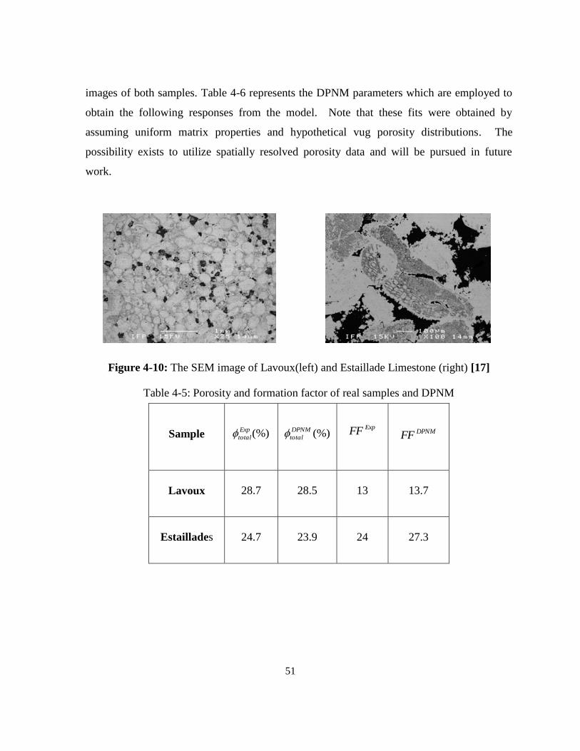
4.2 Verification of the Model

As indicated in Figure 4-12 and Figure 4-14, the dual pore network describes the electrical

resistivity of both Estaillades and Lavoux carbonate samples quite well, as is evident from

comparison with the experimental data of Bauer et al. (Bauer et al. 2011). The DPNM

reproduces the formation factor of both samples (Table 4-5), while being consistent with the

pore size distributions determined by mercury porosimetry. Figure 4-11 illustrates the SEM

51

images of both samples. Table 4-6 represents the DPNM parameters which are employed to

obtain the following responses from the model. Note that these fits were obtained by

assuming uniform matrix properties and hypothetical vug porosity distributions. The

possibility exists to utilize spatially resolved porosity data and will be pursued in future

work.

Figure 4-10: The SEM image of Lavoux(left) and Estaillade Limestone (right) [17]

Table 4-5: Porosity and formation factor of real samples and DPNM

Sample (%)Exp

total (%)DPNM

total ExpFF DPNMFF

Lavoux 28.7 28.5 13 13.7

Estaillades 24.7 23.9 24 27.3

52

Table 4-6: DPNM parameters

Sample (%)vug (%)matrix R 0

mf l (µm)

Lavoux 12.65 28 0.4 0.8 0.4 200

Estaillades 15 30 0.25 0.815 0.7 200

4.2.1 Lavoux Carbonate Sample Verification

Figure 4-12 illustrates the DPNM response for the network of 32x32x32 cells. These

results are consistent with the experimental resistivity response of Lavoux sample [17]. The

total porosity is 28.5%, 12.65% of secondary pore space and 28% of matrix porosity, both

matrix and secondary pore space networks are percolating Figure 4-4 (b). Figure 4-11 shows

the vug distribution used in the model. More than sixty percent of the water is drained

through the secondary porosity, and then the remaining water(less than forty percent) is

drained from the matrix porosity. In experimental pore entry diameter curve the slight

variation in the slope occurs at saturation of about fifty percent. In addition, response in

DPNM is in saturation of about forty percent. In the context of the D-PNM, in the case of

percolating matrix, conduction through the matrix pores causes a leveling off the resistivity

index at lower saturations.

53

Figure 4-11: Vug distribution for Lavoux sample

(a)

54

(b)

Figure 4-12: Lavoux carbonate sample: (a) resistivity index vs. saturation, (b) pore entry

diameter distribution

4.2.2 Estaillades Carbonate Sample

The Estaillades sample is represented by a percolating secondary pore space network

superimposed on non-percolating matrix Figure 4-14 (b).These results are consistent with the

experimental resistivity response of Estaillades sample [17]. Figure 4-15 illustrates the vug

distribution in this set of parameter. About forty percent of the water is drained through the

secondary porosity and more than sixty percent is drained from the matrix porosity. In the

context of the D-PNM, the curving upwards of the resistivity index near forty percent water

saturation for the Estaillades sample occurs because of increasing resistivity of water

remaining in drained secondary pore spaces. The above mentioned effect is observable

particularly while the matrix porosity is non-percolating.

55

Figure 4-13: Vug distribution for Estaillades sample

(a)

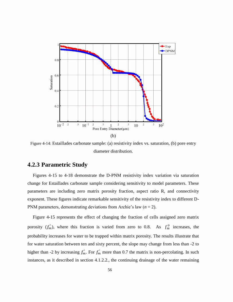
56

(b)

Figure 4-14: Estaillades carbonate sample: (a) resistivity index vs. saturation, (b) pore entry

diameter distribution.

4.2.3 Parametric Study

Figures 4-15 to 4-18 demonstrate the D-PNM resistivity index variation via saturation

change for Estaillades carbonate sample considering sensitivity to model parameters. These

parameters are including zero matrix porosity fraction, aspect ratio R, and connectivity

exponent. These figures indicate remarkable sensitivity of the resistivity index to different D-

PNM parameters, demonstrating deviations from Archie’s law (n = 2).

Figure 4-15 represents the effect of changing the fraction of cells assigned zero matrix

porosity ), where this fraction is varied from zero to 0.8. As o

mf increases, the

probability increases for water to be trapped within matrix porosity. The results illustrate that

for water saturation between ten and sixty percent, the slope may change from less than -2 to

higher than -2 by increasing . For

more than 0.7 the matrix is non-percolating. In such

instances, as it described in section 4.1.2.2., the continuing drainage of the water remaining

57

in the corners of vugs causes a sharp increase in electrical resistivity since there is no

alternative conduction pathway.

Figure 4-15: Effect of zero matrix porosity fractions

Figure 4-16 indicates the effect of changing the ratio R in the model of Estaillades

carbonate. The sharp increase in the curve is the effect of draining water from the corners of

secondary pore space (vugs and throats). The throats have a significant effect, because they

control the capillary pressure and, therefore the corner saturation when the secondary

porosity is first invaded. A higher value of R signifies throats of greater side length and

therefore a greater contribution to conductivity from water remaining in the corners

following non-wetting phase invasion into the secondary pore spaces. Accordingly, RI

becomes more sensitive to changes in water saturation as R increases, and effect more

evident when parallel conduction pathways (conduction through matrix) are scarce.

58

Figure 4-16: Effect of size ratio R

The effect of changing the connectivity exponent ω is depicted in Figure 4-17. ω is the

parameter controlling the probability of communication of adjacent vugs via secondary pore

space (vug throats), influencing significantly (albeit not exclusively) percolation of the

secondary porosity. We compared the responses for three different values of ω. Two effects

are observed as ω is increased from 0.7 to 1. Firstly, small negative deviations from Archie’s

law are seen at high saturation, understood as weaking of the dependence of resistivity on

total saturation as drainage of water from a more connected network of vugs takes place.

This is followed by a strenghtening of the dependence of D-PNM resistivity on water

saturation over a saturation range when conduction is dependent on water in the corners of

drained vugs. Such strengthening, manifested as a sharp increase in RI, is more pronounced

when the vugs are mostly connected to eachother.

59

Figure 4-17: Effect of connectivity exponent

Figure 4-18 demonstrates a similar effect when the shape parameter of the distribution of

secondary porosity is changed (see section 3.1.2.). Increasing the shape parameter decreases

the skew of the vug side distribution, which increases the probability of connection between

two adjacent vugs and thus shifts the RI curves to the left.

60

Figure 4-18: Effect of the shape of vug size distribution

61

Chapter 5

Conclusions

In this study, we have developed a realistic yet tractable dual pore network model (D-

PNM) to relate electrical resistivity at partial saturation to key aspects of the pore structure of

carbonate rocks. The model could be calibrated to the experimental data of the capillary

pressure and electrical resistivity for two carbonate rock samples extensively studied in the

literature. The D-PNM developed has to the following key features, all of which are

important for the description of electrical resistivity: (1) it enables independent control of the

connectivity and percolation of primary and secondary porosity, and thus accounts for the

effects of fluid trapping, (2) it considers the effect of remaining fluid in the corners of

drained secondary pores, (3) it can accommodate distribution and spatial structure of primary

and secondary porosity. Specifically, the work presented in this thesis allows the following

conclusions to be drawn from the data presented:

The non-Archie behavior of bending down in the resistivity curve occurs even in

one cell response. In a single cell, this behavior is associated with conduction via

water in the corners of the secondary pore space.

The D-PNM electrical responses have been classified into nine different types

based on the degree of percolation and relative amount of matrix and secondary

porosity. It is observed that the model is capable of stylistically reproducing all

deviations from Archie’s law.

Non-Archie behavior of two different carbonate rocks (Estaillades and Lavoux

carbonates) has been modeled by the D-PNM in a manner consistent with

experimental data from literature [17]. The properties of these two rocks (formation

factor and total porosity) were consistent with the experimental data.

62

Parametric studies have been conducted to explore the sensitivity of the D-PNM to

key parameters: connectivity exponent, secondary porosity aspect ratio R, fraction

of cells with zero matrix porosity and shape of vug size distribution. Model

response is sensitive to all parameters considered. This indicates the potential to

use the D-PNM for parameter estimation, using a minimum of petrophysical

information (3D maps of porosity from microtomographic images and mercury

intrusion capillary pressure data)

Quantitative interpretation of the non-Archie behavior of the electrical resistivity of

vuggy carbonates appears possible in the context of the D-PNM proposed, at a

small fraction of the computational and information cost of alternative models

attempting to reproduce in great detail the microstructure of carbonate rocks using

microtomographic data.

63

Chapter 6

Recommendations

The model has been verified for two different carbonate samples on the basis of

electrical and capillary properties. The DPNM could be further interrogated for

consistency (i) with other petrophysical properties, such as absolute and relative

permeability and (ii) with experimental data for other carbonate rock samples.

The model should be used for inverse modeling of experimental capillary pressure

and electrical resistivity data for the purpose of best-fitting model parameters using

an optimization approach conditioned on micro-tomographic data. This will relax

the assumption of uniform matrix porosity and will enable incorporation of spatial

structure of the secondary porosity, both of which are important aspects of

heterogeneity.

Water remaining in the corners of the secondary pore space has an important effect

on electrical resistivity. This effect is presently taken into account by assuming

simple corner geometry. A richer behavior would likely emerge if fractal geometry

were to be considered. Further, modeling in this direction seems warranted.

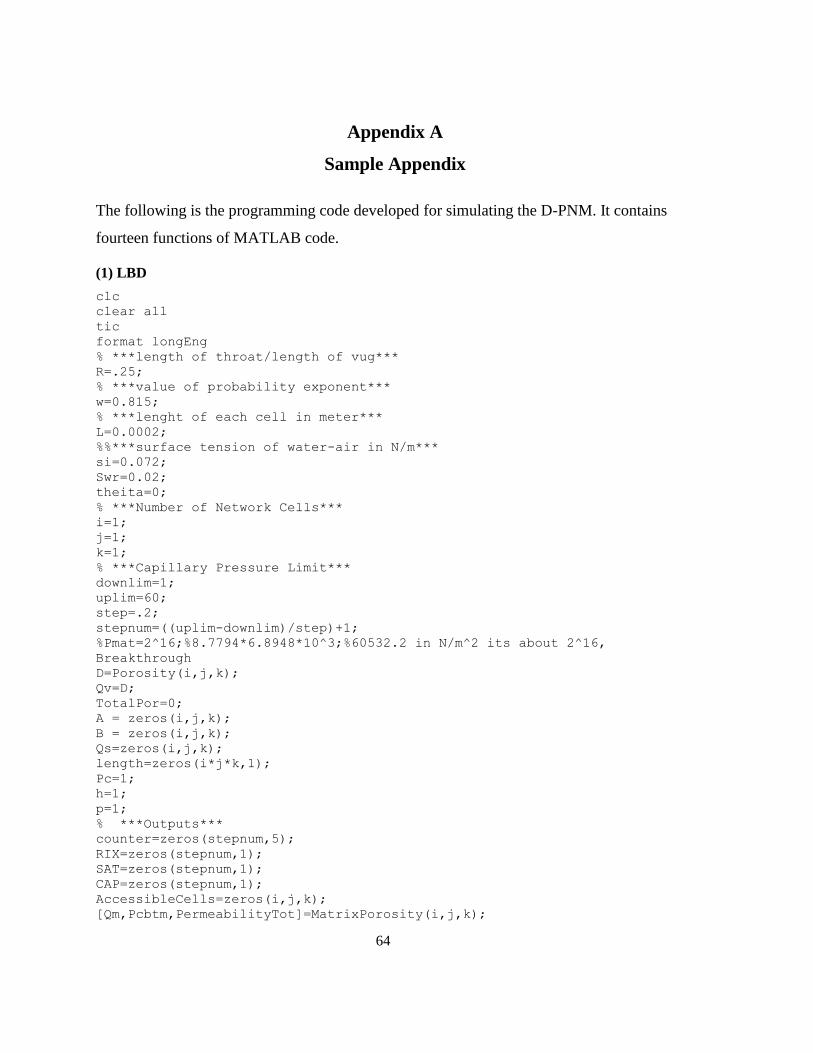
64

Appendix A

Sample Appendix

The following is the programming code developed for simulating the D-PNM. It contains

fourteen functions of MATLAB code.

(1) LBD

clc clear all tic format longEng % ***length of throat/length of vug*** R=.25; % ***value of probability exponent*** w=0.815; % ***lenght of each cell in meter*** L=0.0002; %%***surface tension of water-air in N/m*** si=0.072; Swr=0.02; theita=0; % ***Number of Network Cells*** i=1; j=1; k=1; % ***Capillary Pressure Limit*** downlim=1; uplim=60; step=.2; stepnum=((uplim-downlim)/step)+1; %Pmat=2^16;%8.7794*6.8948*10^3;%60532.2 in N/m^2 its about 2^16,

Breakthrough D=Porosity(i,j,k); Qv=D; TotalPor=0; A = zeros(i,j,k); B = zeros(i,j,k); Qs=zeros(i,j,k); length=zeros(i*j*k,1); Pc=1; h=1; p=1; % ***Outputs*** counter=zeros(stepnum,5); RIX=zeros(stepnum,1); SAT=zeros(stepnum,1); CAP=zeros(stepnum,1); AccessibleCells=zeros(i,j,k); [Qm,Pcbtm,PermeabilityTot]=MatrixPorosity(i,j,k);

65

for x=1:i for y=1:j for z=1:k Q=D(x,y,z); Prs(h,1)=Q; A(x,y,z)= NR(Q,R,L); length(h,1)=A(x,y,z); B(x,y,z)=R*A(x,y,z);%in meter h=h+1; end end end %hist(Prs) %xlswrite('filemm',length) %disp(A) %disp(B) %***Finding the Toatal Porosity of Network*** for x=1:i for y=1:j for z=1:k Qs(x,y,z)=(Qv(x,y,z)*(1-Qm(x,y,z)))+Qm(x,y,z); TotalPor=Qs(x,y,z)+TotalPor; end end end [ ms,FF ] = mfactor(

i,j,k,A,Pc,Pcbtm,Qm,R,Swr,si,theita,L,AccessibleCells,TotalPor); %display(Qs) % ***Get the Inlet Surface from the User*** [NCI,NCJ,NCK]=PCONECTION(w,D,i,j,k); M=input('Please Enter the Inlet Surface:x, y or z:','s'); % ***Finding the Total Saturation of Network*** for t=downlim:step:uplim%log2 of input capilarry pressue(2^9<Pcbtv<2^12,

Pcbtm=2^16) %disp(t) Pc=2^t; [Pcbt,opcell,nvug,nmat]=OPCELL(Pcbtm,B,Pc,i,j,k,theita,si); lbd=opcell; % ***show the open cells with the cappilary pressure*** %OPCEL(X), X is cappillary pressure in N/m^2 [AccessibleCells,numac]=ACCESS(lbd,NCI,NCJ,NCK,M,Pc); counter(p,1)=Pc; counter(p,2)=i*j*k; counter(p,3)=nvug; counter(p,4)=nmat; counter(p,5)=numac; [RI,ROs]=RENORM(i,j,k,A,Pc,Pcbtm,Qm,R,Swr,si,theita,L,AccessibleCells); SatCell=zeros(i,j,k); SigmaSat=0; SatC=CellSat(Pcbtm,Qm,Qs,Swr,si,theita,L,A,B,D,Pc,i,j,k,AccessibleCells ); for x=1:i for y=1:j for z=1:k

66

SatCell(x,y,z)=SatC(x,y,z).*Qs(x,y,z); SigmaSat=SatCell(x,y,z)+SigmaSat; end end end %display(SatCell) %display(SigmaSat) TotalSat=1-(SigmaSat/TotalPor); PorosityTotal=TotalPor/(i*j*k); subplot(3,1,1); loglog(TotalSat,RI,'r*') %hold on %subplot(2,1,2);loglog(TotalSat,Pc,'m+') RIX(p,1)=RI; SAT(p,1)=TotalSat; CAP(p,1)=Pc; p=p+1; hold on end hold on % subplot(2,1,1) % plot(log(CAP),1-SAT,'*'); hold on [yint,dyint,xx,DIAMS]=xxsplines( CAP,SAT,si,theita ); xx=xx'; toc

(2) Matrix Porosity

function [ Qm,Pcbtm,PermeabilityTot ] = MatrixPorosity( i,j,k) r=rand(i,j,k); m=0; n=0; qq=0.3; Pcbtm = zeros(i,j,k); Perm = zeros(i,j,k); TotalPerm=0; for x=1:i for y=1:j for z=1:k if r(x,y,z)<=0.7 m=m+1; r(x,y,z)=qq.*(10^-20); end if r(x,y,z)>0.7 n=n+1; r(x,y,z)=qq; end Perm(x,y,z)=1859.3*(r(x,y,z).^1.732); TotalPerm=TotalPerm+Perm(x,y,z);%mDarcy Pcbtm(x,y,z)=20*6.8948*10^3*(12.6991)*(Perm(x,y,z).^-0.369); end end end

67

Qm=r; PermeabilityTot=TotalPerm/(i*j*k); end

(3) NR

function [ a ] = NR( Q ,R,L) %***This function calculate a side lenght of cubic vug a(x) %by using Q(vug porosity), R(b/a) and L(size of block) %as a given value*** %L=0.01;%in meter X(1)=Q; E(1)=1; i=1; j=1; %Newton-Raphson while E(i)>.000005; i=i+1; X(i)=X(i-1)-((1-3*R^2).*X(i-1).^3+3*R^2.*X(i-1).^2-Q)/... (3*(1-3*R^2).*X(i-1).^2+6*R^2.*X(i-1)); E(i)=abs((X(i)-X(i-1))/X(i)); j=j+1; k=0; if j>50 k=1; error('FAIL TO CONVERGE') break end if k==0; a=X(i)*L; end end

(4) MFACTOR

function [ ms,FF ] = mfactor(

i,j,k,A,Pc,Pcbtm,Qm,R,Swr,si,theita,L,AccessibleCells,TotalPor) %***Calculating the formation factor*** %F=Qs^-ms %F=RDPN(%100)/RWater ro=20;%ohm-meter Rwater=ro*(j*L)/((i*L)*(k*L)); [ ~,R0s ] = RENORM(i,j,k,A,Pc,Pcbtm,Qm,R,Swr,si,theita,L,AccessibleCells); FF=R0s/Rwater; QS=TotalPor/(i*j*k); ms=-log(FF)/log(QS); end

(5) Pconnection

function [ NCI,NCJ,NCK ] = PCONECTION(w,D,i,j,k) %***Probability of finding connection between two neighbouring blocks*** %w=0.7; %value of probability exponent

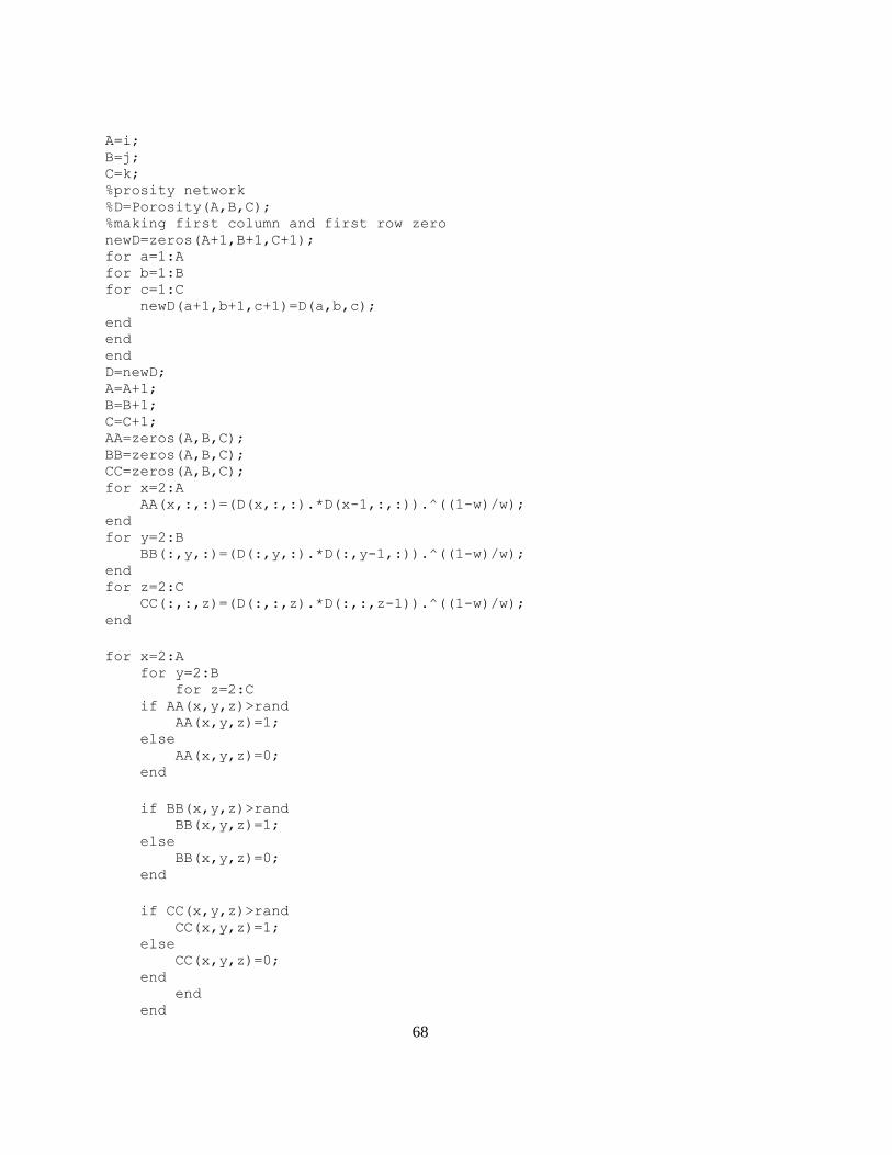
68

A=i; B=j; C=k; %prosity network %D=Porosity(A,B,C); %making first column and first row zero newD=zeros(A+1,B+1,C+1); for a=1:A for b=1:B for c=1:C newD(a+1,b+1,c+1)=D(a,b,c); end end end D=newD; A=A+1; B=B+1; C=C+1; AA=zeros(A,B,C); BB=zeros(A,B,C); CC=zeros(A,B,C); for x=2:A AA(x,:,:)=(D(x,:,:).*D(x-1,:,:)).^((1-w)/w); end for y=2:B BB(:,y,:)=(D(:,y,:).*D(:,y-1,:)).^((1-w)/w); end for z=2:C CC(:,:,z)=(D(:,:,z).*D(:,:,z-1)).^((1-w)/w); end

for x=2:A for y=2:B for z=2:C if AA(x,y,z)>rand AA(x,y,z)=1; else AA(x,y,z)=0; end

if BB(x,y,z)>rand BB(x,y,z)=1; else BB(x,y,z)=0; end

if CC(x,y,z)>rand CC(x,y,z)=1; else CC(x,y,z)=0; end end end

69

end NCI=AA;%above NCJ=BB;%left NCK=CC;%inside end

(6) OPCELL

function [Pcbt,opcell,nvug,nmat] = OPCELL(Pcbtm,B,Pc,i,j,k,theita,si) openpres=Pc;%in N/m^2 %***Finding the constant dimensionless Pc prime*** %theita=0; lambda=1; nvug=0; nmat=0; %si=0.072;%%surface tension of water-air in N/m F1=((pi/2)-(2*theita))-(2*sqrt(2)*cos(theita)*sin((pi/4)-theita)); F2=(0.5*sin((pi/2)-2*theita))+((sin((pi/4)-theita))^2)-((pi/4)-theita); %a=F1*F2; %b=2*(lambda+1)*F2*cos(theita); %c=lambda*F1; %P=[a b c]; %Rprime=min(roots(P)); Rprime=0.5302; Pcp=(((lambda+1)*cos(theita))+(Rprime*F1))/(lambda-(Rprime^2*F2)); Pcbt = zeros(i,j,k); opcell=zeros(i,j,k); %***Finding the Breakthroughthrough Capillary Pressure for Each Cell*** %disp(D) %pres=zeros(i*j*k,1); for x=1:i; for y=1:j; for z=1:k Pcbt(x,y,z)=(Pcp*si*2)/B(x,y,z);%in N/m^2 if (openpres > Pcbt(x,y,z) )&&(openpres<Pcbtm(x,y,z)) opcell(x,y,z)=1; nvug=nvug+1; elseif openpres > Pcbtm(x,y,z) opcell(x,y,z)=2; nmat=nmat+1; end %hist(log2(Pcbt)) %set(gca,'XScale','log2') %plot(Pcapmx,0,'*') end end end end

(7) ACCESS

function [ ACS,numac ] = ACCESS(lbd,NCI,NCJ,NCK,M,Pc ) %***Finding the Accessible Clusters***

70

%disp(D) numac=0; [cls]=SK(lbd,NCI,NCJ,NCK); [p, q, r]=size(lbd); if M=='x' n=q*r; N=zeros(1,n); k=1; for b=1:q for c=1:r if cls(1,b,c)~=0 N(1,k)=cls(1,b,c); M=zeros(1,k); for m=1:k M(1,m)=N(1,m); end k=k+1; end end end for a=2:p for b=1:q for c=1:r if cls(a,b,c)~=0 if any(M==cls(a,b,c))==0 cls(a,b,c)=0; end end end end end s=0; for b=1:q for c=1:r if s==0 if cls(p,b,c)~=0 if any(M==cls(p,b,c))~=0 % disp('Percolation') % disp(Pc) s=1; end end end end end elseif M=='y' n=p*r; N=zeros(1,n); k=1; for a=1:p for c=1:r if cls(a,1,c)~=0 N(1,k)=cls(a,1,c);

71

M=zeros(1,k); for m=1:k M(1,m)=N(1,m); end k=k+1; end end end for a=1:p for b=2:q for c=1:r if cls(a,b,c)~=0 if any(M==cls(a,b,c))==0 cls(a,b,c)=0; end end end end end s=0; for a=1:p for c=1:r if s==0 if cls(a,q,c)~=0 if any(M==cls(a,q,c))~=0 %disp('Percolation') %disp(Pc) s=1; end end end end end elseif M=='z' n=p*q; N=zeros(1,n); k=1; for a=1:p for b=1:q if cls(a,b,1)~=0 N(1,k)=cls(a,b,1); M=zeros(1,k); for m=1:k M(1,m)=N(1,m); end numac=k; k=k+1;

end end end for a=1:p for b=1:q

72

for c=2:r if cls(a,b,c)~=0 if any(M==cls(a,b,c))==0 cls(a,b,c)=0; else numac=numac+1; end end end end end s=0; for a=1:p for b=1:q if s==0 if cls(a,b,r)~=0 if any(M==cls(a,b,r))~=0 %disp('Percolation') % disp(Pc) s=1; end end end end end end ACS=cls; end

(8) RENORM

function [ RI,R0s ] =

RENORM(i,j,k,A,Pc,Pcbtm,Qm,R,Swr,si,theita,L,AccessibleCells) %UNTITLED2 Summary of this function goes here % Detailed explanation goes here [Rcell,R0]=CellResis(i,j,k,A,Pc,Pcbtm,Qm,R,Swr,si,theita,L,AccessibleCells

); R=zeros(i,j,k); p=i; while p>1 for x=1:2:i for y=1:2:j for z=1:2:k R1=R0(x,y,z); R2=R0(x,y+1,z); R3=R0(x+1,y,z); R4=R0(x+1,y+1,z); R5=R0(x,y,z+1); R6=R0(x,y+1,z+1); R7=R0(x+1,y,z+1); R8=R0(x+1,y+1,z+1); RoutKirch= Kirchhoffs(R1,R2,R3,R4,R5,R6,R7,R8); R0(x,y,z)=RoutKirch/2; R1=Rcell(x,y,z);

73

R2=Rcell(x,y+1,z); R3=Rcell(x+1,y,z); R4=Rcell(x+1,y+1,z); R5=Rcell(x,y,z+1); R6=Rcell(x,y+1,z+1); R7=Rcell(x+1,y,z+1); R8=Rcell(x+1,y+1,z+1); RoutKirch= Kirchhoffs(R1,R2,R3,R4,R5,R6,R7,R8); R(x,y,z)=RoutKirch/2; end end end R0((1:i/2),(1:j/2),(1:k/2))=R0(1:2:x,1:2:y,1:2:z); Rcell((1:i/2),(1:j/2),(1:k/2))=R(1:2:x,1:2:y,1:2:z); R0=R0(1:i/2,1:j/2,1:k/2); Rcell=Rcell(1:i/2,1:j/2,1:k/2); i=i/2;j=j/2;k=k/2; p=i; end RI=Rcell/R0; R0s=R0*2; %disp(RI) end

(9) CELLSAT

function [ Snw] =

CellSat(Pcbtm,Qm,Qs,Swr,si,theita,L,A,B,D,Pc,i,j,k,AccessibleCells ) [Pcbt,opcell]=OPCELL(Pcbtm,B,Pc,i,j,k,si,theita); Qv=D; Snw=ones(i,j,k); Pcprime=zeros(i,j,k); Rprime=zeros(i,j,k); Vco1=zeros(i,j,k); Vco2=zeros(i,j,k); Vco=zeros(i,j,k); Vthroat=zeros(i,j,k); Satvug=zeros(i,j,k); Smnw=zeros(i,j,k); %***Matrix Saturation*** for x=1:i for y=1:j for z=1:k if Pc>Pcbtm(x,y,z) if AccessibleCells(x,y,z)~=0 Pstar=Pc./Pcbtm(x,y,z); Sweff=Pstar^(-0.6666); Smw=(Sweff*(1-Swr))+Swr;%each cell matrix saturation Smnw(x,y,z)=1-Smw;%nonwetting phase sat Pcprime(x,y,z)=(Pc*B(x,y,z))/(2*si); Rprime(x,y,z)=1/Pcprime(x,y,z); F2=(0.5*sin((pi/2)-2*theita))+((sin((pi/4)-theita))^2)-

((pi/4)-theita);

74

%Find the non occupied volume Vco1(x,y,z)=((B(x,y,z)/2).*Rprime(x,y,z)).^2.*((L-

A(x,y,z))/2)*F2*24;

Vco2(x,y,z)=((A(x,y,z)/2).*Rprime(x,y,z)).^2.*A(x,y,z)*F2*8; Vco(x,y,z)=Vco1(x,y,z)+Vco2(x,y,z); Vthroat(x,y,z)=(6*(B(x,y,z).^2).*((L-

A(x,y,z))/2))+A(x,y,z).^3; Satvug(x,y,z)=1-(Vco(x,y,z)/Vthroat(x,y,z)); end end

%***Vug Saturation*** if (Pc>Pcbt(x,y,z))&&(Pc<Pcbtm(x,y,z)) if AccessibleCells(x,y,z)~=0 Pcprime(x,y,z)=(Pc*B(x,y,z))/(2*si); Rprime(x,y,z)=1/Pcprime(x,y,z); F2=(0.5*sin((pi/2)-2*theita))+((sin((pi/4)-theita))^2)-((pi/4)-

theita); %Find the non occupied volume Vco1(x,y,z)=((B(x,y,z)/2).*Rprime(x,y,z)).^2.*((L-

A(x,y,z))/2)*F2*24; Vco2(x,y,z)=((A(x,y,z)/2).*Rprime(x,y,z)).^2.*A(x,y,z)*F2*8; Vco(x,y,z)=Vco1(x,y,z)+Vco2(x,y,z); Vthroat(x,y,z)=(6*(B(x,y,z).^2).*((L-A(x,y,z))/2))+A(x,y,z).^3; Satvug(x,y,z)=1-(Vco(x,y,z)/Vthroat(x,y,z)); end end

%***each cell saturation*** Snw(x,y,z)=((Qv(x,y,z).*Satvug(x,y,z))+((1-

Qv(x,y,z)).*Qm(x,y,z).*Smnw(x,y,z)))... ./Qs(x,y,z); end end end %Qss=Qs %MatrixSaturation=Smw; %VugSaturation=Satvug %Satcell=Sw end

(10) CELLRESIS

function[Rcell,R0]=CellResis(i,j,k,A,Pc,Pcbtm,Qm,R,Swr,si,theita,L,Accessi

bleCells) ro=20;%ohm-meter m=2 ; n=2; Pcp=1.8862; F2=(0.5*sin((pi/2)-2*theita))+((sin((pi/4)-theita))^2)-((pi/4)-theita); Pcbt=zeros(i,j,k); Rvug=zeros(i,j,k);

75

Rmatrix=zeros(i,j,k); Rcell=zeros(i,j,k); R0vug=zeros(i,j,k); R0matrix=zeros(i,j,k); R0=zeros(i,j,k); Rprime=zeros(i,j,k); Pcprime=zeros(i,j,k); B=R.*A; for x=1:i for y=1:j for z=1:k Pcbt(x,y,z)=(Pcp*si*2)/B(x,y,z); R0vug(x,y,z)=(ro/2)*(((L-A(x,y,z))/B(x,y,z).^2)+(1/A(x,y,z))); Rvug(x,y,z)=R0vug(x,y,z); R0matrix(x,y,z)=(ro/2)*(((L-A(x,y,z))./((L^2)-

(B(x,y,z).^2)))+... (A(x,y,z)./((L^2)-(A(x,y,z).^2)))) *Qm(x,y,z).^-m; Rmatrix(x,y,z)=R0matrix(x,y,z); if Pc>Pcbtm(x,y,z) if AccessibleCells(x,y,z)~=0 Pstar=Pc./Pcbtm(x,y,z); Sweff=Pstar^(-0.6666); Smw=(Sweff*(1-Swr))+Swr;%each cell matrix saturation water Rmatrix(x,y,z)=(ro/2)*(((L-A(x,y,z))/((L^2)-

(B(x,y,z).^2)))+... (A(x,y,z)/((L^2)-(A(x,y,z).^2)))).*Smw^-n*Qm(x,y,z).^-

m; Pcprime(x,y,z)=(Pc*B(x,y,z))/(2*si); Rprime(x,y,z)=1/Pcprime(x,y,z); At=(((B(x,y,z)/2).*Rprime(x,y,z)).^2)*F2*4; Av=(((A(x,y,z)/2).*Rprime(x,y,z)).^2)*F2*4; Rvug(x,y,z)=(ro/2)*(((L-A(x,y,z))/At)+(A(x,y,z)/Av)); end end if (Pc>Pcbt(x,y,z))&&(Pc<Pcbtm(x,y,z)) if AccessibleCells(x,y,z)~=0 Pcprime(x,y,z)=(Pc*B(x,y,z))/(2*si); Rprime(x,y,z)=1/Pcprime(x,y,z); At=(((B(x,y,z)/2).*Rprime(x,y,z)).^2)*F2*4; Av=(((A(x,y,z)/2).*Rprime(x,y,z)).^2)*F2*4; Rvug(x,y,z)=(ro/2)*(((L-A(x,y,z))/At)+(A(x,y,z)/Av)); end end if A(x,y,z)==0 Rcell(x,y,z)=Rmatrix(x,y,z); R0(x,y,z)=R0matrix(x,y,z); else Rcell(x,y,z)= 1/((1/(Rvug(x,y,z)))+(1/Rmatrix(x,y,z))); R0(x,y,z)=1/((1/(R0vug(x,y,z)))+(1/R0matrix(x,y,z))); end %RI(x,y,z)=Rcell(x,y,z);%R0(x,y,z); end end

76

end %display(R0) %display(Rcell) end

(11) KIRSHOF

function [ RoutKirch ] = Kirchhoffs(R1,R2,R3,R4,R5,R6,R7,R8) %This fuction get 8 resistivity as an input and simplify it to one resis %by using renormalization method %***step1***

%left side A=R3; B=R1; C=R5; D=R7; %right side E=R4; F=R2; G=R6; H=R8; %center cubic %outside I=R1+R3; J=R1+R2; K=R2+R4; L=R3+R4; %inside M=R5+R7; N=R5+R6; O=R6+R8; P=R7+R8; %side Q=R1+R5; R=R3+R7; S=R2+R6; T=R4+R8; %LU Factoriztion Method a=[1/J+1/I+1/B+1/Q -1/J -1/I 0 -1/Q 0 0 0; -1/J 1/J+1/K+1/F+1/S 0 -1/K 0 -1/S 0 0; -1/I 0 1/I+1/L+1/A+1/R -1/L 0 0 -1/R 0; 0 -1/K -1/L 1/K+1/L+1/T+1/E 0 0 0 -1/T; -1/Q 0 0 0 1/Q+1/N+1/M+1/C -1/N -1/M 0; 0 -1/S 0 0 -1/N 1/S+1/N+1/O+1/G 0 -1/O; 0 0 -1/R 0 -1/M 0 1/D+1/R+1/M+1/P -1/P; 0 0 0 -1/T 0 -1/O -1/P 1/T+1/O+1/P+1/H]; b=[1/B;0;1/A;0;1/C;0;1/D;0]; %Y=linsolve(a,b) V=mldivide(a,b); I2=V(2)/F; I4=V(4)/E; I6=V(6)/G;

77

I8=V(8)/H; I=I2+I4+I6+I8; %I1=(1-V(1))/B; %I3=(1-V(3))/A; %I5=(1-V(5))/C; %I7=(1-V(7))/D; %Iplus=I1+I3+I5+I7; RoutKirch=1/I; end

(12) SK

function [ cls ] =SK(lbd,NCI,NCJ,NCK) %***Hoshen & Kopelman algorithm with considering the probability of %connections*** %Probability of finding connection between two neighbouring blocks [i, j, k]=size(lbd); newlabel=0; cntr=1; %making first column and first row zero newlbd=zeros(i+1,j+1,k+1); for a=1:i for b=1:j for c=1:k newlbd(a+1,b+1,c+1)=lbd(a,b,c); end end end lbd=newlbd; i=i+1; j=j+1; k=k+1; %define cluster size array q=i*j*k; csize=zeros(q,1); %Matrix travese for z=2:k for x=2:i for y=2:j if lbd(x,y,z)==2 lbdx=lbd(x-1,y,z); lbdy=lbd(x,y-1,z); lbdz=lbd(x,y,z-1); if lbdx==2 NCI(x,y,z)=1; end if lbdy==2 NCJ(x,y,z)=1; end if lbdz==2 NCK(x,y,z)=1; end end end

78

end end for z=2:k for x=2:i for y=2:j if lbd(x,y,z)==2 lbd(x,y,z)=1; end end end end

for z=2:k for x=2:i for y=2:j if lbd(x,y,z)~=0 lbdx=lbd(x-1,y,z); lbdy=lbd(x,y-1,z); lbdz=lbd(x,y,z-1); above=lbdx*NCI(x,y,z); left=lbdy*NCJ(x,y,z); inside=lbdz*NCK(x,y,z); if (above~=0)&&(left~=0)&&(inside~=0) if above==left==inside lbd(x,y,z)=above; if csize(above,1)>0 csize(above,1)=csize(above,1)+1; end else mn1=min(above,left); mn2=min(above,inside); mx1=max(above,left); mx2=max(above,inside); mn=min(mn1,mn2); avg=max(mn1,mn2); mx=max(mx1,mx2); lbd(x,y,z)=mn; if csize(mn,1)>0 csize(mn,1)=csize(mn,1)+1; end s=csize(mx,1); csize(mx,1)=-mn; if s<0 n=1; while n<1000 if s<0 v=abs(s); s=csize(abs(s),1); csize(v,1)=-mn; n=n+1; elseif s>0 break; end

79

end end s=csize(avg,1); csize(avg,1)=-mn; if s<0 n=1; while n<1000 if s<0 v=abs(s); s=csize(abs(s),1); csize(v,1)=-mn; n=n+1; elseif s>0 break; end end end end elseif (above~=0)&&(left==0)&&(inside==0) lbd(x,y,z)=above; if csize(above,1)>0 csize(above,1)=csize(above,1)+1; end elseif (above==0)&&(left~=0)&&(inside==0) lbd(x,y,z)=left; if csize(left,1)>0 csize(left,1)=csize(left,1)+1; end elseif (above==0)&&(left==0)&&(inside~=0) lbd(x,y,z)=inside; if csize(inside,1)>0 csize(inside,1)=csize(inside,1)+1; end elseif (above~=0)&&(left~=0)&&(inside==0) mn=min(above,left); mx=max(above,left); lbd(x,y,z)=mn; if csize(mn,1)>0 csize(mn,1)=csize(mn,1)+1; end s=csize(mx,1); csize(mx,1)=-mn; if s<0 n=1; while n<1000 if s<0 v=abs(s); s=csize(abs(s),1); csize(v,1)=-mn; n=n+1; elseif s>0 break; end

80

end end elseif (above==0)&&(left~=0)&&(inside~=0) mn=min(left,inside); mx=max(left,inside); lbd(x,y,z)=mn; if csize(mn,1)>0 csize(mn,1)=csize(mn,1)+1; end s=csize(mx,1); csize(mx,1)=-mn; if s<0 n=1; while n<1000 if s<0 v=abs(s); s=csize(abs(s),1); csize(v,1)=-mn; n=n+1; elseif s>0 break; end end end elseif (above~=0)&&(left==0)&&(inside~=0) mn=min(above,inside); mx=max(above,inside); lbd(x,y,z)=mn; if csize(mn,1)>0 csize(mn,1)=csize(mn,1)+1; end s=csize(mx,1); csize(mx,1)=-mn; if s<0 n=1; while n<1000 if s<0 v=abs(s); s=csize(abs(s),1); csize(v,1)=-mn; n=n+1; elseif s>0 break; end end end else newlabel=newlabel+1; lbd(x,y,z)=newlabel; csize(newlabel,1)=cntr; end end end

81

end end %display(lbd) %display(csize) %check the csize of clusters for z=2:k for x=2:i for y=2:j if lbd(x,y,z)~=0 d=csize(lbd(x,y,z),1); if d<0 m=1; while m<1000 if d<0 e=abs(d); d=csize(abs(d),1); if e==abs(d) lbd(x,y,z)=e; end m=m+1; elseif d>0 lbd(x,y,z)=e; break; end end end end end end end new2lbd=zeros(i-1,j-1,k-1); for a=2:i for b=2:j for c=2:k new2lbd(a-1,b-1,c-1)=lbd(a,b,c); end end end cls=new2lbd; end

(13) TRIDIAG

function x = Tridiag(e,f,g,r) % x = Tridiag(e,f,g,r): % Tridiagonal system solver. % input: % e = subdiagonal vector % f = diagonal vector % g = superdiagonal vector % r = right hand side vector % output: % x = solution vector n=length(f);

82

% forward elimination for k = 2:n factor = e(k)/f(k-1); f(k) = f(k) - factor*g(k-1); r(k) = r(k) - factor*r(k-1); end % back substitution x(n) = r(n)/f(n); for k =n-1:-1:1 x(k) = (r(k)-g(k)*x(k+1))/f(k); end

(14) XXSPLINES

function [ yint,dyint,xx,DIAMS] = xxsplines(CAP,SAT,si,theita) %function yint = mysplines(x,y,xx) DIAMS = (10^6)*4*si*cos(theita)./CAP; x=flipud(log10(DIAMS)); y=flipud(1-SAT);

nsplines = length(x)-1;%Number of cubic splines to be determined

for i = 1:nsplines h(i) = x(i+1)-x(i); d(i) = y(i); end

iknots = nsplines -1; %Number of internal knots

%Set up the tridiagonal system of equations e(1) = 0; g(iknots)=0; for i = 2:iknots e(i) = h(i); end for i = 1:iknots f(i) = 2*(h(i)+h(i+1)); r(i) = 6*((y(i+2)-y(i+1))/h(i+1)-(y(i+1)-y(i))/h(i)); end for i = 1:iknots-1 g(i) = h(i+1); end

%Solve the tridiagonal system to get second derivative at the internal %knots sol = Tridiag(e,f,g,r);

S=zeros(nsplines+1, 1);

for i = 2:nsplines S(i) = sol(i-1); end

83

for i = 1:nsplines b(i) = S(i)/2; a(i) = (S(i+1)-S(i))/(6*h(i)); c(i) = (y(i+1)-y(i))/h(i) - (2*h(i)*S(i)+h(i)*S(i+1))/6; end

%Use cubic splines to interpolate

xx = (min(x)+1):.1:(max(x)-1); yint = zeros(length(xx),1); dyint=zeros(length(xx),1);

for j = 1:length(xx) %for each xx where interpolation is needed found = 0; %Variable to indicate when proper spline has been

found i = 1; while found==0 %Search for the interval containing xx to locate

proper spline if x(i)<=xx(j) && xx(j)<=x(i+1) yint(j) = a(i)*(xx(j)-x(i))^3+b(i)*(xx(j)-x(i))^2+... c(i)*(xx(j)-x(i))+d(i); dyint(j) = 3*a(i)*(xx(j)-x(i))^2+2*b(i)*(xx(j)-x(i))+c(i); found = 1; else i = i+1; end end end

subplot(3,1,2) plot(x,y,'ro',xx,yint); subplot(3,1,3) plot(xx,dyint) end

84

Bibliography

[1] Schlumberger, “Schlumberger Market Analysis,” 2007. [Online]. Available:

http://www.slb.com/.

[2] G. Archie, “The Electrical Resistivity Log as an Aid in Determining Some Reservoir

Characteristics,” Pet. Trans. AIME, vol. 146, pp. 54–62, 1942.

[3] J. R. Dixon and B. F. Marek, “The Effect of Bimodal Pore Size Distribution on Electrical

Properties of Some Middle Eastern Limestones,” Soc. Pet. Eng. 20601, pp. 743–750, Apr.

1990.

[4] J. W. Focke and D. Munn, “Cementation Exponents in Middle Eastern Carbonate Reservoirs,”

Soc. Pet. Eng. 13735, pp. 155–167, 1985.

[5] S. Saner, A. Al-Harthi, and M. T. Htay, “Use of Tortuosity for Discriminating Electro-facies

to Interpret the Electrical Parameters of Carbonate Reservoir Rocks,” J. Pet. Sci. Eng., vol. 16,

no. 4, pp. 237–249, Dec. 1996.

[6] M. Fleury, “Resistivity in Carbonates: New Insights,” Proc. SPE Annu. Tech. Conf. Exhib.,

pp. 1–12, Sep. 2002.

[7] G. S. Padhy, M. A. Ioannidis, C. Lemaire, and M. Coniglio, “Measurement and Interpretation

of Non-Archie Resistivity Behavior in Model and Reak Vuggy Carbonates,” Soc. Core Anal.,

vol. 11, pp. 1–11, 2006.

[8] M. J. Petricola and M. Walfa, “Effect of Microporosity in Carbonates: Introduction of a

Versatile Saturation Equation,” Soc. Pet. Eng., pp. 607–615, 1995.

[9] A. I. M. Dicker and W. A. Bemelmans, “Models for Simulating the Electrical Resistance of

Porous Media,” SPWLA 25th Annu. Logging Symp., pp. 1–12, 1984.

[10] M. Han, M. Fleury, and P. Levitz, “Effect of the Pore Structure on Resistivity Index Curves,”

Soc. Core Anal., vol. 34, no. 1997, pp. 1–12, 2007.

[11] P. N. Sen, “Resistivity of Partially Saturated Carbonate Rocks with Microporosity,”

Geophisics, vol. 62, no. 2, pp. 415–425, 1997.

[12] M. A. Ioannidis, M. J. Kwiecien, and I. Chatzis, “Electrical Conductivity and Percolation

Aspects of Statistically Homogeneous Porous Media,” Transp. Porous Media, vol. 29, pp. 61–

83, 1997.

[13] B. Montaron, “Connectivity Theory – A New Approach to Modeling Non-Archie Rocks,”

Petrophysics, vol. 50, no. 2, 2009.

85

[14] D. Zhou, S. Arbabi, and E. H. Stenby, “A Percolation Study of Wettability Effect on the

Electrical Properties of Reservior Rocks,” Transp. Porous Media, vol. 29, no. 1, pp. 85–98,

1997.

[15] G. S. Padhy, M. A. Ioannidis, and C. Lemaire, “Interpretation of the Non-Archie Resistivity

Behaviour in Vuggy Carbonates: Use of Pore Structure Parameters,” SPWLA Middle East Reg.

Symp., pp. 1–14, 2007.

[16] M. Han, S. Youssef, E. Rosenberg, M. Fleury, and P. Levitz, “The Effect of the Porous

Structure on Resistivity Index Curves. an Experimental and Numerical Study.,” SPWLA 49th

Annu. Logging Symp., pp. 1–10, 2008.

[17] D. Bauer, S. Youssef, M. Han, S. Bekri, E. Rosenberg, M. Fleury, and O. Vizika, “From

Computed Microtomography Images to Resistivity Index Calculations of Heterogeneous

Carbonates Using a Dual-porosity Pore-network Approach: Influence of percolation on the

electrical Transport Properties,” Phys. Rev. E, vol. 84, no. 1, p. 011133, Jul. 2011.

[18] M. A. Ioannidis and I. Chatzis, “A Dual-Network Model of Pore Structure for Vuggy

Carbonates,” Proc. Annu. Symp. Soc. Core Anal., 2000.

[19] F. L. . Dullien, Porous Media: Fluid Transport and Pore Structure. Academic Press, 1991, p.

574.

[20] M. A. Ioannidis, “On the Description of Capillary and Transport Phenomena in Heterogeneous

Porous Media,” University of Waterloo, Waterloo, Ontario, 1993.

[21] R. Defay and I. Prigogine, Surface Tension and Adsorption. London: London: Longmans,

1966.

[22] I. Chatzis, “A Network Approach to Analyze and Model Capillary and Transport Phenomena

in Porous Media,” University of Waterloo, 1980.

[23] B. Legait, “Laminar Flow of Two Phases Through a Capillary Tube with Variable Square

Cross-section,” J. Colloid Interface Sci., vol. 96, no. 1, pp. 28–38, Nov. 1983.

[24] A. Y. Dandekar, Petroleum Reservoir Rock and Fluid Properties. CRC Press, 2013, p. 544.

[25] J. Hoshen and R. Kopelman, “Percolation and cluster distribution. I. Cluster multiple labeling

technique and critical concentartion algorithm,” Phys. Rev. B, vol. 14, no. 8, pp. 3438–3445,

1976.

[26] M. L. Aldridge, “A Finite State Machine Approach to Cluster Identification Using the

Hoshen-Kopelman Algorithm,” The University of Tennessee, Knoxville, 2008.

[27] M. A. Ioannidis and I. Chatzis, “Network Modeling of Pore Structure and Transport Properties

of Porous Media,” Chem. Eng. Sci., vol. 48, no. 5, pp. 951–972, 1993.

86

[28] Y. Nakashima and T. Nakano, “Accuracy of Formation Factors for Three-dimensional Pore-

scale Images of Geo-materials Estimated by Renormalization Technique,” J. Appl. Geophys.,

vol. 75, no. 1, pp. 31–41, Sep. 2011.

[29] P. R. King, “The Use of Renormalization for Calculating Effective Permeability,” Transp.

Porous Media, vol. 4, pp. 37–58, 1989.

[30] D. Bauer, S. Youssef, M. Fleury, S. Bekri, E. Rosenberg, and O. Vizika, “Improving the

Estimations of Petrophysical Transport Behavior of Carbonate Rocks Using a Dual Pore

Network Approach Combined with Computed Microtomography,” Transp. Porous Media,

vol. 94, no. 2, pp. 505–524, Jan. 2012.

dual pore network model of electrical resistivity for

Documents