AD-Ai18 234 TRINITY COLL DUBLIN (IRELAND) DEPT OF CIVIL ENGINEERING FIG 20/11NUMERICAL METHODS FOR CREEP ANALYSIS IN GEOTECHNICAL PROBLEMS.(U)DEC 81 T E GLYNN DAERO-76-$-063

UNCLASSIFIED NL*2 lfllflllf//lEEEEEEllEEEEEEEEEEIhEIIEEEEEIIEEEEEEEEEEEEIEIIIEEEEEIIEEIEEEEEEEEEEEEEIIEIIEEEEIIIIEE

-: NUMERICAL METHODS FOR CREEP ANALYSISIN

GEOTECHNICAL PROBLEMS

FINAL TECHNICAL REPORT

byq

Civil Engineering ItT. E. GLYNN Department

Trinity College

To

EUROPEAN RESEARCH OFFICE

United States Army

0.GRANTEE UNIVERSITY Of DUBLINS ENGINEERING SCHOOLTRINITY. COLLEGE

GRANT NO. DAERO76 -G-063December 1981.

*z08"16 4

Project Title PAVEMENT RESEARCH

Report Title

NUMERICAL METHODS FOR CREEP ANALYSIS IN

GEOTECHNICAL PROBLEMS

FINAL TECHNICAL REPORT

BY

T,E. GLYNN DEPARTMENT OF CIVIL ENGINEERING

TRINITY COLLEGE

Grantee University of DublinEngineering SchoolTrinity College

Dublin.

The research reported in this document has been madepossible through the support and sponsorship of theUnited States Army through its European ResearchOffice.

DIM3 S A !S2!it-IT~~ - ue

App rdfrpi', eeB

___________ I

SYNOPSIS

This report presents the results of a theoretical study of

inelastic material behaviour produced by static loading on

a viscous continuum. A number of issues are addressed in

an attempt to introduce inelastic behaviour into piecewise

numerical methods. Methods based on similitude and direct

integraLion of Lhe displacement field are investigated.

Potential field theory is invoked as a means of describing

stress distributions which are assumed invariant with respect

to time of straining the material. No attempt has been

made to include forced flow, strain hardening or frictional

material properties. The analysis is restricted to slow

deformations and results in a line integral for conversion

of strain rate to displacement as a function of time of

straining. The interpretdtion of experimental data is

viewed from the stand-point of functional analysis as it

is felt that this branch of mathematics has unexplored

implications in the study of creep of deformable bodies.

U~ i- ) Ac . j.JJ

Ac S40 t r. I .. ... ---

- ..

' f.LAi

ACKNOWLEDGEMENTS

The author gratefully acknowledges the sponsorship of the

U.S. Army through its European Research Office. Personal

thanks is extended to the former chief scientist of E.R.O.

Dr. Hoyt Lemons and to the present chief scientist Warren E.

Grabau for their guidance and co-operation.The encouragement afforded by Professor W. Wright, Head of the

Engineering School, to conduct fundamental research is

appreciated.

Assistance with closed form solutions and reference sources

given by mathematician Victor Graham is gratefully acknowledged.

Thanks to Professor J.G.Byrne, Head of the Computer Science

Department, for facilitating development of computer programs.

Programming assistance was provided by Mrs. Rosemary Welsh and

by Gary Lyons who also draughted the diagrams in the report.

(ii)

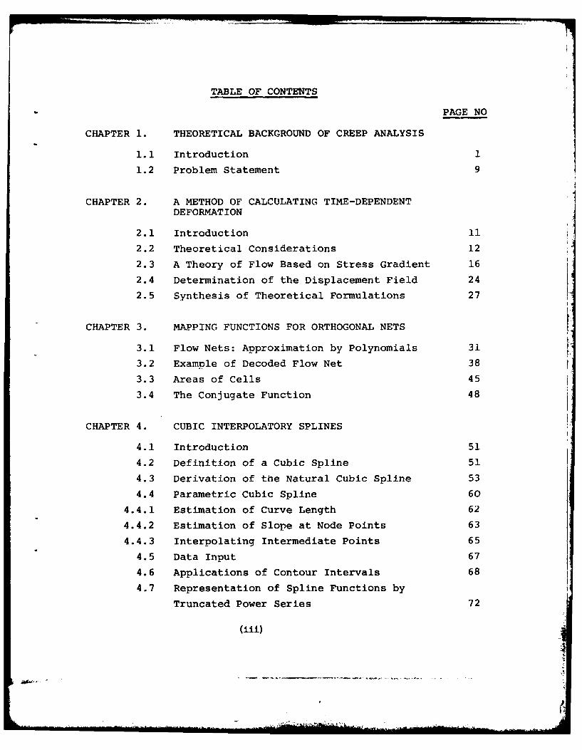
TABLE OF CONTENTS

PAGE NO

CHAPTER 1. THEORETICAL BACKGROUND OF CREEP ANALYSIS

1.1 Introduction 1

1.2 Problem Statement 9

CHAPTER 2. A METHOD OF CALCULATING TIME-DEPENDENTDEFORMATION

2.1 Introduction 11

2.2 Theoretical Considerations 12

2.3 A Theory of Flow Based on Stress Gradient 16

2.4 Determination of the Displacement Field 24

2.5 Synthesis of Theoretical Formulations 27

CHAPTER 3. MAPPING FUNCTIONS FOR ORTHOGONAL NETS

3.1 Flow Nets: Approximation by Polynomials 31

3.2 Example of Decoded Flow Net 38

3.3 Areas of Cells 45

3.4 The Conjugate Function 48

CHAPTER 4. CUBIC INTERPOLATORY SPLINES

4.1 Introduction 51

4.2 Definition of a Cubic Spline 51

4.3 Derivation of the Natural Cubic Spline 53

4.4 Parametric Cubic Spline 60

4.4.1 Estimation of Curve Length 62

4.4.2 Estimation of Slope at Node Points 63

4.4.3 Interpolating Intermediate Points 65

4.5 Data Input 67

4.6 Applications of Contour Intervals 68

4.7 Representation of Spline Functions by

Truncated Power Series 72(iii) .

......................

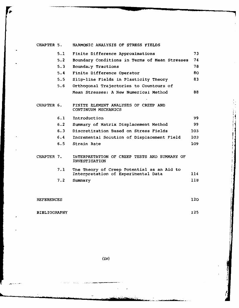
CHAPTER 5. HARMONIC ANALYSIS OF STRESS FIELDS

5.1 Finite Difference Approximations 73

5.2 Boundary Conditions in Terms of Mean Stresses 74

5.3 Boundaiy Tractions 78

5.4 Finite Difference Operator 80

5.5 Slip-line Fields in Plasticity Theory 83

5.6 Orthogonal Trajectories to Countours of

Mean Stresses: A New Numerical Method 88

CHAPTER 6. FINITE ELEMENT ANALYSES OF CREEP ANDCONTINUUM MECHANICS

6.1 Introduction 99

6.2 Summary of Matrix Displacement Method 99

6.3 Discretization Based on Stress Fields 103

6.4 Incremental Solution of Displacement Field 103

6.5 Strain Rate 109

CHAPTER 7. INTERPRETATION OF CREEP TESTS AND SUMMARY OFINVESTIGATION

7.1 The Theory of Creep Potential as an Aid toInterpretation of Experimental Data 114

7.2 Summary 118

REFERENCES 120

BIBLIOGRAPHY 125

(iv)

I

CHAPTER 1

THEORETICAL BACKGROUND OF CREEP ANALYSIS

1.1 Introduction

This report covers the period from August 1976 to

December 1981 for research under Grant No. DA ERO-76-

G-063. The object of the research stipulated in the

grant documentation was to compliment earlier experimen-

tal study of flexible pavements by fundamental analysis

of materials under stress. The main objective is to

find solutions for unrestrained flow such as the rutting

of flexible payments and settlement of structures.

The original proposal was accepted 6 August 1976 and

subsequently was the subject of one modification

designated DRXSN-E-AO, of March 1977.

This report presents the results of a theoretical study

of inelastic material behaviour in a stress field

produced by static loading of a viscous continuum.

During the course of the project it transpired that the

original objectives became somewhat eclipsed by theoretical

development of wider scope. Procedures which employ

the mathematical background of continuum mechanics to

the solution of the longstanding engineering problem of

slow creep of materials are described. While the theme

of application to highway engineering underscores the

study in this report the development of ideas is

generalised to encompass a variety of problems in geo-

technical engineering. No attempt has been made to

confine the study to specific materials, but for the

sake of some simplification the discussion of certain

types of inelastic bahaviour have been omitted e.g. flow

of granular materials, strain hardening substances.

(1)

A number of issues are addressed in an attempt to

introduce inelastic behaviour into piecewise nume I

construction of solutions of some generality in th

mechanics of solids. The projec commenced -ith a

review of existing theory and so ition methou to be

found in the extensive literature on creep and plastic

flow. The author's previous experience of unresolved

problems in geotechnical engineering provided motives

and guidance to the ultimate requirements of further

theoretical development. The text will demonstrate

that no definitive line is taken in the preparation of

this report: rather the problem is attacked from a

number of standpoints in a search for common ground of

a unified theory; the problem is treated at different

levels of complexity, but generally the aim is simplific-

ation of existing analytical methods.

These methods comprise classical plasticity which

exhibits path dependent but time independent behaviour;

classical viscoelasticity and creep theory both of which

have path dependent and time dependent components. To

avoid infringing on the technical meaning of visco-

elastic and plastic behaviour the theoretical developments

herein may be described as that which applies to material

in the mastic state e.g. asphalt or remoulded clay. A

brief statement of the classical theories follows.

Plasticity The task of plastic theory is twofold:

first to set up relationships between stress and strain

which describes adequately the observed plastic deformat-

ion of the material in laboratory tests, and second to

(2)

develop techniques for using these relationships in

analysis and design. At least two variants of the

theory are in common usage - the ideal rigid plastic and

the elastoplastic models. These models employ the

concepts of yield surface, associated flow rules and

plastic potential functions. Throughout the theorytime enters as a dummy variable only, while stresses

and deformations are viewed as incremental rather than

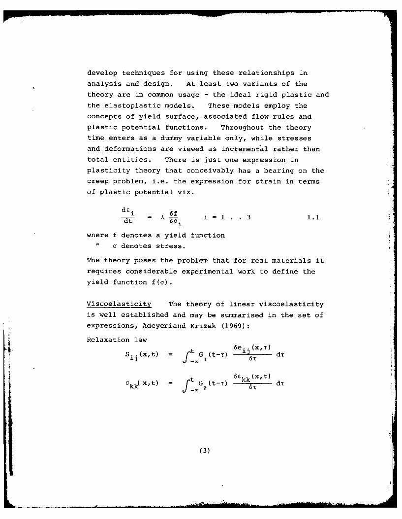
total entities. There is just one expression in

plasticity theory that conceivably has a bearing on the

creep problem, i.e. the expression for strain in terms

of plastic potential viz.

d__- &fdt A I-. i = 1..3 1.11 !

where f denotes a yield tunction" a denotes stress.

The theory poses the problem that for real materials it

requires considerable experimental work to define the

yield function f(a).

Viscoelasticity The theory of linear viscoelasticity

is well established and may be summarised in the set of

expressions, Adeyeriand Krizek (1969):

Relaxation law6ei (x,T)

Si (x,t) G (t-T) d+iOk ~t t _ ,(tT 6T d

6 kk (xt)0~(Xt t i ((t-T) kT dT

(3)

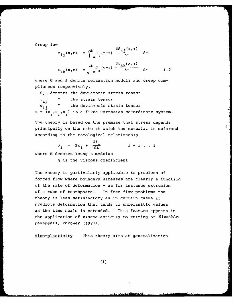
Creep law

e. (x, t) = t-T 6 dTt J (t-T) 6 kk(X'T)

Ckk(x,t) = f- 2 6r dT 1.2

where G and J denote relaxation moduli and creep com-

pliances respectively,

S. denotes the deviatoric stress tensor

E. " the strain tensor1J

e. " the deviatoric strain tensor1J

x = (x ,x ,x ) is a fixed Cartesian co-ordinate system.I 2 3

The theory is based on the premise that stress depends

principally on the rate at which the material is deformed

according to the rheological relationshipde

a F +r-d i = i 3a. = E ..01 1 dt.

where E denotes Young's modulus

n is the viscous coefficient

The theory is particularly applicable to problems of

forced flow where boundary stresses are clearly a function

of the rate of deformation - as for instance extrusion

of a tube of toothpaste. In free flow problems the

theory is less satisfactory as in certain cases it

predicts deformation that tends to unrelasitic values

as the time scale is extended. This feature appears in

the application of viscoelasticity to rutting of flexible

pavements, Thrower (1977).

Viso-plasticity This theory aims at generalisation

(4)

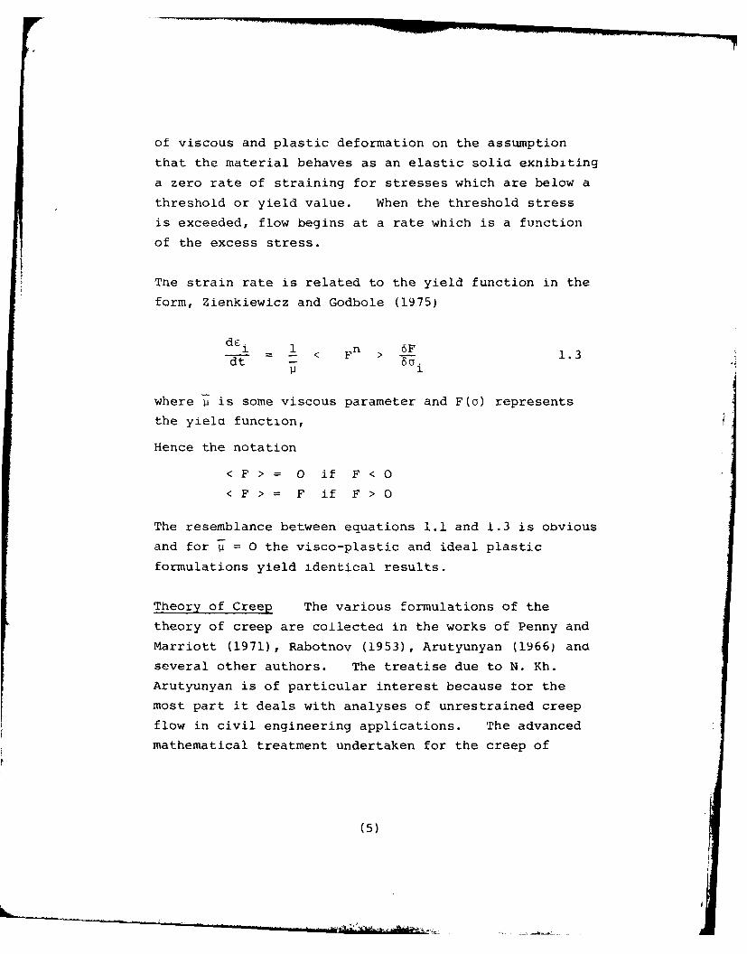
of viscous and plastic deformation on the assumption

that the material behaves as an elastic solia exnibiting

a zero rate of straining for stresses which are below a

threshold or yield value. When the threshold stress

is exceeded, flow begins at a rate which is a function

of the excess stress.

The strain rate is related to the yield function in the

form, Zienkiewicz and Godbole (1975)

Idei 1 FS -- < Fn > 6F 1.3

dt 6oi

where p is some viscous parameter and F(o) representsthe yield function,

Hence the notation

< F > = 0 if F < 0

< F > F if F > 0

The resemblance between equations 1.1 and 1.3 is obvious

and for j = 0 the visco-plastic and ideal plastic

formulations yield identical results.

Theory of Creep The various formulations of the

theory of creep are collected in the works of Penny and

Marriott (1971), Rabotnov (1953), Arutyunyan (1966) and

several other authors. The treatise due to N. Kh.

Arutyunyan is of particular interest because tor the

most part it deals with analyses of unrestrained creep

flow in civil engineering applications. The advanced

mathematical treatment undertaken for the creep of

(5)

* . 4._

concrete structures serves to highlight the complexity

of closed form analysis. However his analysis dis-

closes very practical results which are stated in the

form of theorems thusly:

Theorem 1: If the stress condition of a given body

is produced by the action of external torces, and its

creep function for uniaxial stress C(t,T) is proport-

ional, with constant coefficient of proportionality k°to the creep function for pure shear w(t,T) then the

system of stresses in the body considered coincides

identically with the system of stresses of the

corresponding instantaneous elastic problem.

Theorem 2: If the stress condition in a body either

is constant or changes linearly with the x,y,z co-

ordinates then the stresses in the body during creep

will coincide with the stresses of the corresponding

instantaneous elastic problem for the same body with

different coefficients of lateral compression

V (t) and V (t,T)1 2

The theorems are the outcome of the following

assumptions:

1. The material is regarded as a homogeneous

isotropic body;

2. The relationship between creep deformation and

stresses is linear;

3. The law ot superposition applies to creep

deformation.

4. The functions that characterize the changes in

the coefficient of lateral compression for elastic

deformation and creep deformation are identical,

i.e. v (T) = v (t,T) = v.1 2

(6)

The theorems are interpreted to mean that for un-

restrained slow creeping flow of a material the stress

distribution is not significantly different from that

of the elasticity analysis for steady state boundary

stresses. Of course if the boundary conditions permit

a relaxation of stress anywhere in the domain then the

stress distribution will adjust itself to minimise

stress concentration as is the case with forced fiow.

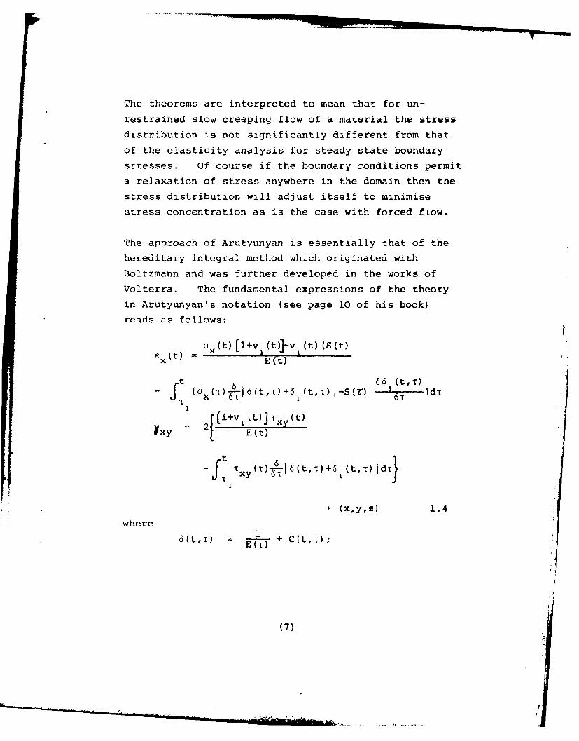
The approach of Arutyunyan is essentially that of the

hereditary integral method which originated with

Boltzmann and was further developed in the works of

Volterra. The fundamental expressions of the theory

in Arutyunyan's notation (see page 10 of his book)

reads as follows:

x(t)[1+v (t)0]-v (t)(S(t)

= E(t)

t 66 (t,T)

f fT 1 {a(T))A-I6(t, z)+6 (t,T)I-S(r) 6T Id

21 (1l+v I(t)] JTx'(t)Ixy E 2t)

Ett)

- Txy(T)T 16(t, )+6 1 (t,T)IdTJ

11

wr (x,y, ) 1.4

where

6(tT) + C(t,T);E(T)

(7)

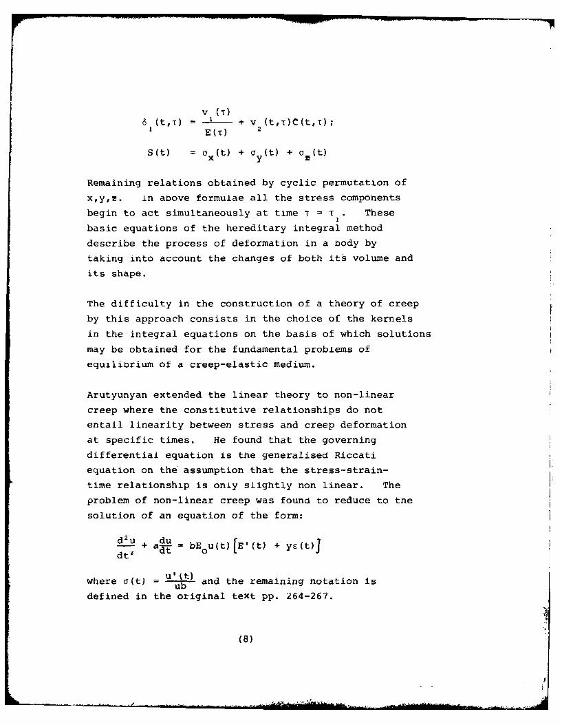
v (ii6 (t,T) 1 + v (t,T)C(t,T);

I E(T) 2

S(t) = (t) + ay(t) + a (t)

Remaining relations obtained by cyclic permutation of

x,y,. in above formulae all the stress components

begin to act simultaneously at time T = T These1

basic equations of the hereditary integral method

describe the process of deformation in a body by

taking into account the changes of both its volume and

its shape.

The difficulty in the construction of a theory of creep

by this approach consists in the choice of the kernels

in the integral equations on the basis of which solutions

may be obtained for the fundamental problems of

equilibrium of a creep-elastic medium.

Arutyunyan extended the linear theory to non-linear

creep where the constitutive relationships do not

entail linearity between stress and creep deformation

at specific times. He found that the governing

differential equation is the generalised Riccati

equation on the assumption that the stress-strain-

time relationship is only slightly non linear. The

problem of non-linear creep was found to reduce to the

solution of an equation of the form:

__u du = Eu + J

dtu + au - bEou(t) E'(t) + ye(t)dt 0

where G(t) = 1u't) and the remaining notation is

defined in the original text pp. 264-267.

(8)

1.2 Probtem Statement

The foregoing review of theory serves to illustrate

the complex nature of any attempt at a closed form

solution of material flow under stress. The formulation

of constitutive stress-strain relations presents a

formidable challenge and to incorporate these in a

boundary value problem is even more exacting. Con-

sequently simplified numerical schemes is a desirable

goal. The fact that the geometrical configuration is

not the prime source of aifficulties suggests that an

analysis developed for a particular geometry may be

readily extendable to other configurations. In this

work the author will concentrate on so-called axisymm-

etric flow problems with the conviction that the develop-

ment could equally apply to plane strain or plane stress

problems albeit with some modification to the analyses.

The axisymmetric case is of common occurrence in

foundation engineering as for instance a circular

storage tank on soft ground, wheel loads on an asphalt

pavement or a circular cofferdam on a compressible

stratum.

The boundary value problem resembles the classical

Boussinesq problem - that of a concentrated or distrib-

uted load on the surface of a semi-infinite half-space.

The thrust of the analysis will be to develop a

numerical technique tor estimating the displacements

beneath a flexible uniformly loaded circular contact

area located on the free boundary of a semi-infinite

half space of homogeneous mastic material. rhe

analysis will delve into flow of thick cylinders subject-

jed to radial forcing pressures (internal and external).

(9)

The task of developing the numerical procedure consists

of the following steps:

i. postulate a mechanism of flow i.e. establish

the geometry ot a plausible mode of flow

deformation.

ii. for an incremented flow of this mechanism

integrate the work dissipated in non-recover-

able deformation over the whole domain (or

a part thereof).

iii. equate the energy supplied by the forcing

pressure to the internal work and hence find

the displacement at the source of the disturb-

ing force as a function of elapsed time of

loading.

iv. investigate method of substituting unprocessed

test data for constitutive relationships in

the analysis.

This scheme constitutes the direct method ot solution

and undoubtedly presents a number of obstacles, but it

is in the spirit of finite element analysis. The

main difficulty is that of specifying the constitutive

relations for detormation in mutually perpendicular

frames of reference i.e. creep laws in terms of stress

invariants. On the other hand an indirect method

based on similitude offers an alternative scheme.

The application of similitude and dimensional analysis

is known to produce practical solutions to otherwise

intractable problems, Glen Murphy (1953). Both

possibilities will be investigated in this report. 4

(10)

CHAPTER 2

A METHOD OF CALCULATING TIME-DEPENDENT DEFORMATION

.1

2.1 Introduction

A draw-back to the methods outlined in Chapter 1 is the

necessity to idealise the response of real materials to

such an extent that the stress-strain relationship fits

into the scheme of a particular theory. The constitutive

equations tend to reflect the type of proposed analysis

rather than actual behaviour i.e. rheological models for

viscoelasticity and flow rules for plasticity. Whereas

the real behaviour may reflect a variety of responses,

the classical theories deal with preselected components.

This approach results in a proliferation of material

parameters, constants and exponents in the effort to fit

experimental data. In what follows the author proposes

an alternative method for the special case of axisymmetric

flow under the action of sustained loading. The basic

idea is to relate the flow problem to an experimental

investigation of a corresponding model of the stress state

using the minimum of data processing of the test results.

In principle the method should prove equally valid for

both linear and non-linear behaviour provided the stress

state can be simulated in the test procedure. To fix

ideas we consider only axisymmetric flow in non-forced

boundary value problems; such processes of flow as

metal forming with dies or presses are excluded at this

stage in the development of the theory.

Initially theoretical aspects are explored, one of which

is presented in this Chapter. The theoretical exercises

are merely the forerunners to the main thrust of the work,

namely the preparation of a scheme for numerical analysis

by computer.

(11)

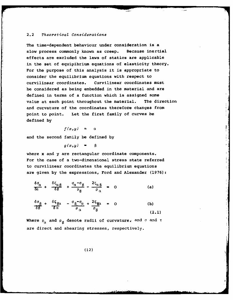
2.2 Theoretical Considerations

The time-dependent behaviour under consideration is a

slow process commonly known as creep. Because inertial

effects are excluded the laws of statics are applicable

in the set of equipibrium equations of elasticity theory.

For the purpose of this analysis it is appropriate to

consider the equilibrium equations with respect to

curvilinear coordinates. Curvilinear coordinates must

be considered as being embedded in the material and are

defined in terms of a function which is assigned some

value at each point throughout the material. The direction

and curvature of the coordinates therefore changes from

point to point. Let the first family of curves be

defined by

f(X,y) = O

and the second family be defined by

g(x,y) 8

where x and y are rectangular coordinate components.

For the case of a two-dimensional stress state referred

to curvilinear coordinates the equilibrium equations

are given by the expressions, Ford and Alexander (1976):

6 + + -0P-'-T--o (a)

6a 6C a-2a .8+ 8ct - ( ,+a 2 , = 0 (b)"a P

(2.1)

Where p and p8 denote radii of curvature, and a and T

are direct and shearing stresses, respectively.

(12)

- - .1

If the coordinate axes are chosen to coincide with the

directions of principal velocity components, then for

materials that exhibit sliding on planes inclined at 45

degrees to the principal planes, the equations of

equilibrium in two dimensions along lines of maximum

shear stress can be written in the form, Kuske and

Robertson (1974)

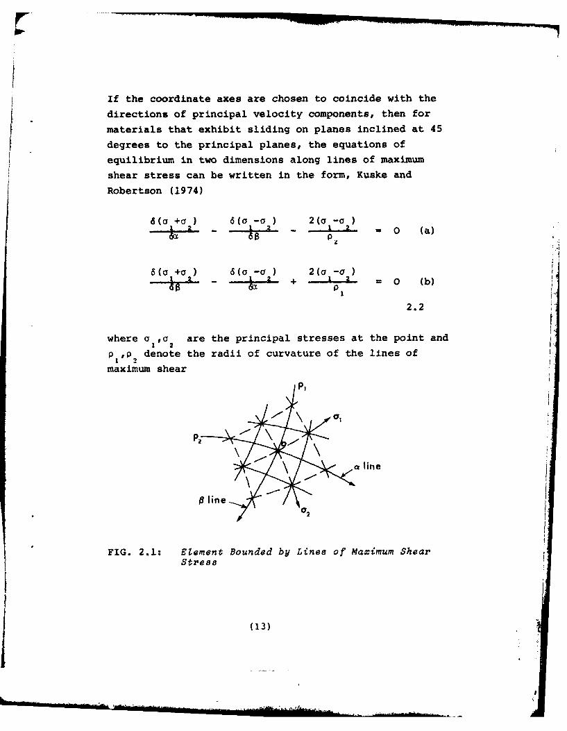
6(O +a ) 6(a -0 ) 2(a -a- _ = 0 (a)

Pz

6(a +) 6(a -a) 2( -a)_ + P = 0 (b)

2.2

Iwhere a ,a are the principal stresses at the point and1 2 Jp , denote the radii of curvature of the lines of

maximum shear

2 a line

FIG. 2.1: Element Bounded by Lines of Maximum ShearStress

(13)

Equation 2.2 provides the equilibrium conditions forthe state of stress shown in Fig. 2.1. This state

consists of the distributions of the mean normal stressand shears along the trajectories of the curvilinear

coordinate system. The stresses at any point within acell reduce to the mean normal stress and the maximum

shear stresses. If we confine the analysis herein tomaterials that flow along planes of maximum shear stressthe net is geometrically an orthogonal mesh. Materials

that possess a Coulomb frictional component are thusexcluded. In the notation of the slip-line theory ofplasticity the geometry is termed an O,8 net. Thei,8 lines can be assigned curvilinear coordinate valuesaccording to scale of plot but one of the lines - the0 line - has the physical significance that it is thecontour of constant normal stress. The 0 - lines arereadily determined as the contours of mean stress forboundary value problems by solution of Laplace's

equation viz.

+ (62 + 62 6 + 0(ci2 2 i+ - ) (a= )-)( °) 2.3a

826X 2 6Y 2 X 2.3

which follows from the invariance of the Laplacian

under transformation of coordinate axes. The equation

2.3 provides the basis for the photoelastic technique

because it implies that stress distribution is independentof the elastic constants of a homogeneous medium. The

(14)

- - '- .--- "-- ---- -.- - __ ___ ____ ___ ____ ___ ____ ___ _'

conjugate function gives the velocity characteristics

a - lines*. It would be a simple matter to plot the

locations of the a - lines if the shear stress

component could be used as an argument of Laplace's

equation, but since this is not the case harmonic

analysis only partially solves the problem of plotting

the slip-line field. The method of stream functions

has been used to find the geometry of the a - lines

separately from the 8 - lines by many investigators

in the field of fluid mechanics. In Chapter 5 of

this report, a method of locating the a - linesis presented.

* The term velocity characteristic is borrowed fromplasticity theory notwithstanding the fact that thegoverning equation 2.3 is elliptic.

(15

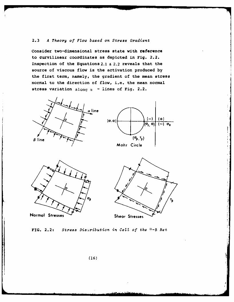
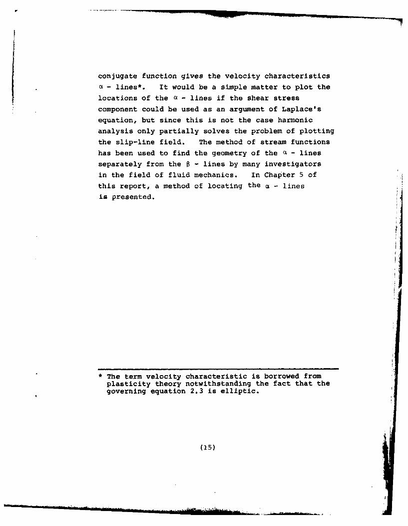
2.3 A Theory of Flow based on Stress Gradient

Consider two-dimensional stress state with reference

to curvilinear coordinates as depicted in Fig. 2.2.

Inspection of the Equations 2.1 & 2.2 reveals that thesource of viscous flow is the activation produced by

the first term, namely, the gradient of the mean stress

normal to the direction of flow, i.e. the mean normal

stress variation along a - lines of Fig. 2.2.

(a0 ( .

Mohr Circle

Normal Stresses Shear Stresses

FIG. 2.2: Stress Die.;ribution in Cell of the a-B Net

(16)

Equilibrium is preserved by the shear stress distribution

on intersecting trajectories as shown by the remaining

terms in the equations. In particular for large radii

of curvature of the trajectories the third term of

Equation 2.2 makes only a small contribution to equilibrium.

Now in a viscous continuum the shearing stresses are not

able to completely restrain permanent deformation once

the material has absorbed the elastic strain energy of

the stress state. Thus the phenomenon of creep ensues

or for certain boundary conditions a relaxation of stress

occurs.

The stress gradient along a flow path bounded by two

- lines is induced by the boundary traction because

the source is the external pressure on the zone bounded

by the same c - lines. The task is to relate the creep

in a model test to the stress gradient in the test and

subsequently to use the correlation for the purpose of

predicting flow in a prototype of the boundary value

problem. To accomplish the transition from model to

prototype it is essential that a unique expression of

the stress gradient be found. If the material behaviour

is linear the so-called unique expression need only be

determined for a single value of the stress state, but

for non-linear material a relationship over a range of

values of stress presumably is required. Such a

unique relationship will advance the theory to the

extent that it provides the link between driving forces

in model and prototype.

(17)

In the search for a unique correlating function the

author was attracted to the properties of the Laplace

transform. It is well known that the transform confers

the capability of distinguishing between functions which

produce the same value for their integrals over some

one interval. By definition we have the Laplace

transform with independent parameter p.

L{f(x)} = f=f(x)ePXdx 2.4

Clearly it is not appropriate to assign values to p

if we are searching for a unique expression in the

hope that a function such as the distribution of stress

gradient can be characterised by a single numerical

value. These considerations have led to the intro-

duction of a special function which bears resemblance

to Laplace transformation formulae; it has the same

property - that of attenuating the function towards the

end of its domain. The proposed function has the form

x-ab-x-x

S which replaces e P of the Laplace transform.

By analogy we can write for a flow path the unique

expression for distribution of f(x) as follows:

x-a

G{f(x)} = jf(x)e- Xdx

[a, b] 2.5

where a and b are the extrernal points of path p.

(18)

lj--boutndory loading.

cross section entry.

ne. flw tube

(19)ne

The correspondence between prototype and model can now

be postulated by assuming that for equal values of G

and the same area subjected to surface traction the

power expended in producing permanent deformation is

identical; and where the G function is different for

prototype and model the boundary velocities for the

prototype follow from similitude according to the

relationship:

GaV G P- AV 2.6

M Mn

where o denotes the driving stress on the boundary

L7 denotes velocity at the source

and subscripts p and m mean prototype and model,

respectively.

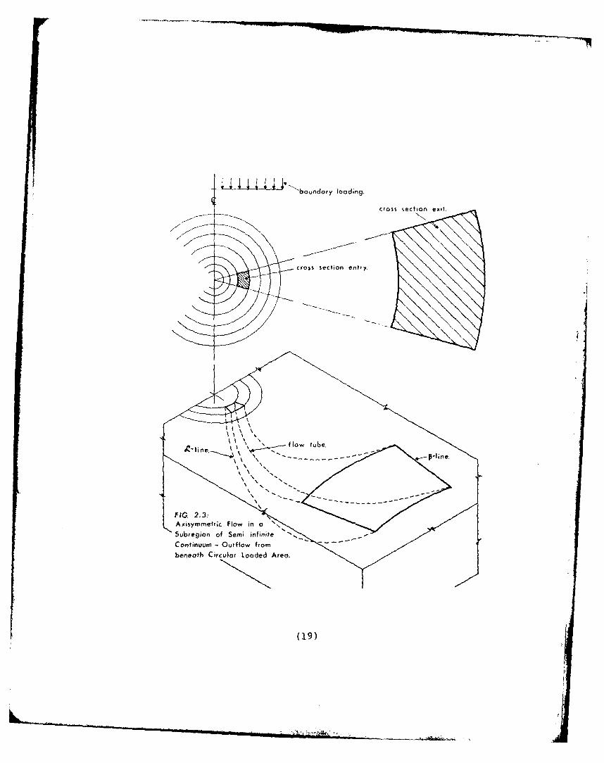
To illustrate the physical meaning of Equation 2.6 we

take for our model the radial flow in the wall of a

thick cylinder under internal pressure and for the

prototype the axially symmetric deformation of a semi-

infinite viscous continum subjected to uniform pressure

on a circular contact area as shown in Fig. 2.3. To

achieve a correspondence we must compare the G-values

on paths that have corresponding stress states.

Firstly consider the case of linear material behaviour.

An expansion test on a thick cylinder will provide the

informa ntityon 2.6 because vhe only un-

known quantity is the velocity (v p the velocity will

in general be a function of time and hence displacements

will need to be determined by integration over an

interval of time or alternatively as a set of Riemann

sums. Second for non-linear materials the only

(20)

.....__,_.. .....______"_____________.__.. -- . .. I

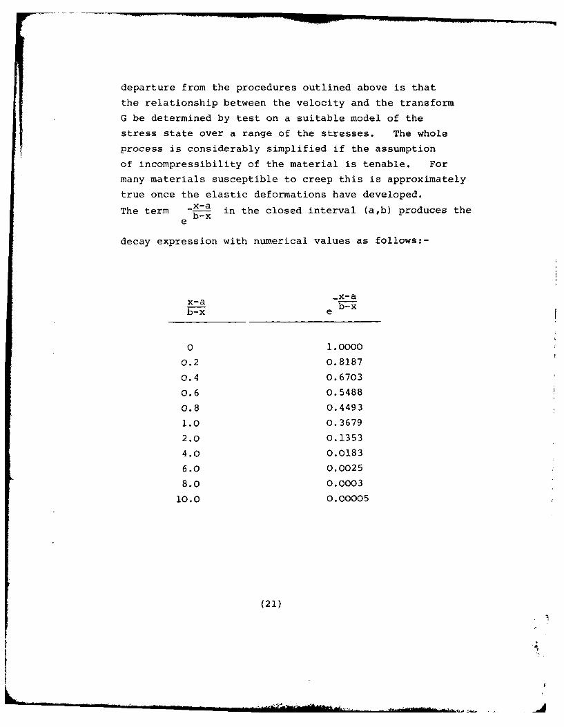
departure from the procedures outlined above is that

the relationship between the velocity and the transform

G be determined by test on a suitable model of the

stress state over a range of the stresses. The whole

process is considerably simplified if the assumption

of incompressibility of the material is tenable. For

many materials susceptible to creep this is approximately

true once the elastic deformations have developed.

The term in the closed interval (a,b) produces theThe term b-xe

decay expression with numerical values as follows:-

_x-ax-a b-xb-x e

0 1.0000

0.2 0.8187

0.4 0.6703

0.6 0.5488

0.8 0.4493

1.0 0.3679

2.0 0.1353

4.0 0.0183

6.0 0.0025

8.0 0.0003

10.0 0.00005

(21)

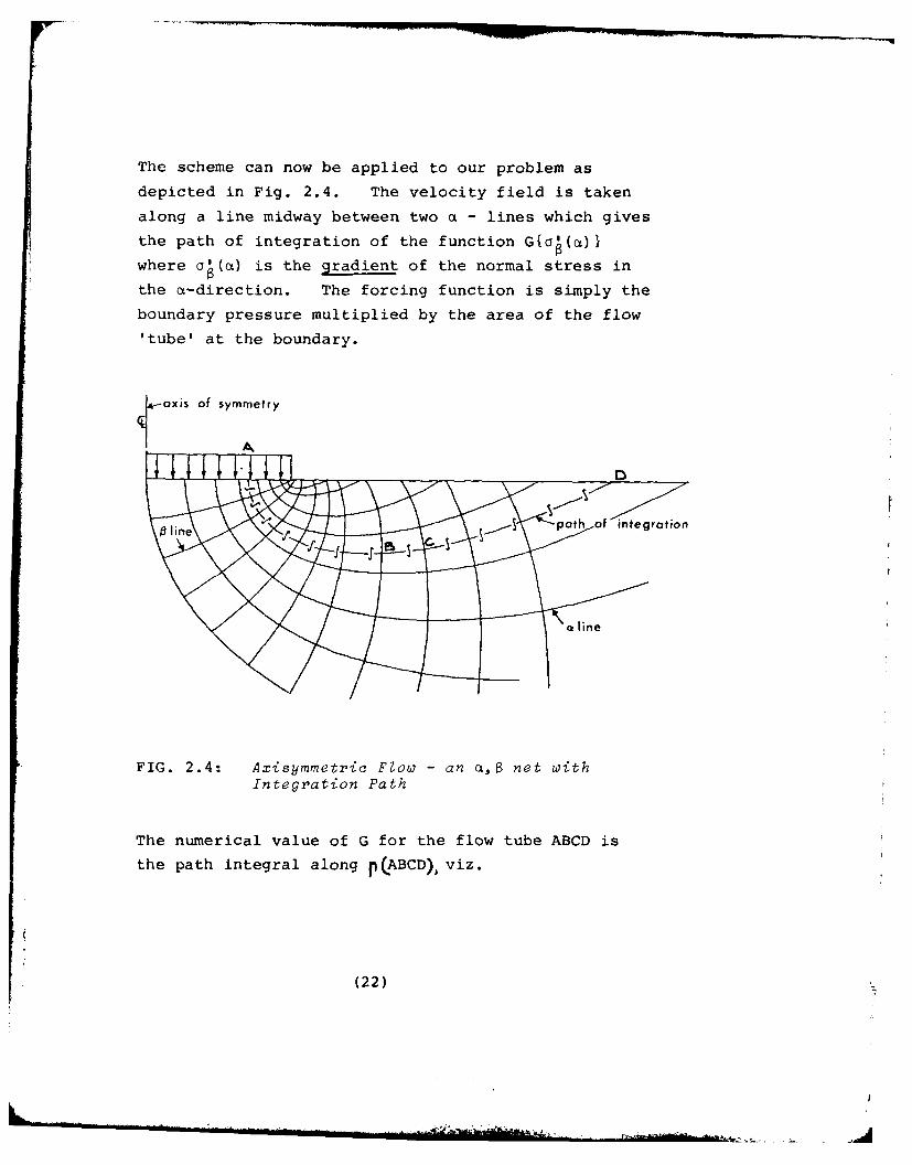
The scheme can now be applied to our problem as

depicted in Fig. 2.4. The velocity field is taken

along a line midway between two a - lines which gives

the path of integration of the function G{oa(a)}

where a'(a) is the gradient of the normal stress in

the a-direction. The forcing function is simply the

boundary pressure multiplied by the area of the flow

'tube' at the boundary.

oxis of symmetry

io Qline

FIG. 2.4: Axisymmetric Flow - an a,lS net withIntegration Path

The numerical value of G for the flow tube ABCD is

the path integral along p(ABCD) viz.

(22)

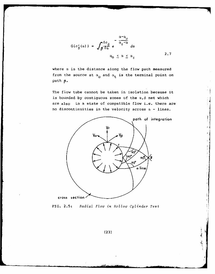
0F60 a -acz-c

Ga ()Ie dcx

ct ac< a 2.7

where a is the distance along the flow path measured

from the source at ao and at is the terminal point on

path p.

The flow tube cannot be taken in isolation because it

is bounded by contiguous zones of the a, net which

are also in a state of compatible flow i.e. there areno discontinuities in the velocity across a - lines.

path of integration

FIG. 2.5: Radial Flow in Hollow Cylinder Test

(23)

2.4 Determination of the Displacement Field

If a material is uncompressible the volume occupied is

constant; the quantity of material which enters a sub-

region is equal to that which leaves it according to

the continuity equation of fluid mechanics

t~)6v

6VX + __) + z = o 2.96X 6y 6Z

The movement of the material can be described in

either Eularian or Lagrangian coordinates; in any

case the relationship between the two systems is well

established, Hodge pp. 143-144.

Due to the comparatively small scale of movements in

a highly viscous medium the Lagrangian approach is

deemed adequate for tracking the progress of flow from

one zone to another; the change in stress gradiant is

sufficiently small to warrant the adoption of a fixed

reference frame. Thus we wlll focus on the relationship

that expresses the displacements caused by flow of

material into and out of a cell of a fixed a,1 net.

The displacements are to be determined along the median

path which is midway between adjacent a - lines, i.e.

the path p shown Fig. 2.6.

The method proposed is to use the properties of the

Jacobian functional derivative for comparison of areas

in the two-dimensional net and the relationship between

curvilinear and rectangular coordinates for the third

dimension of the flow tube. The constant volume

(24)

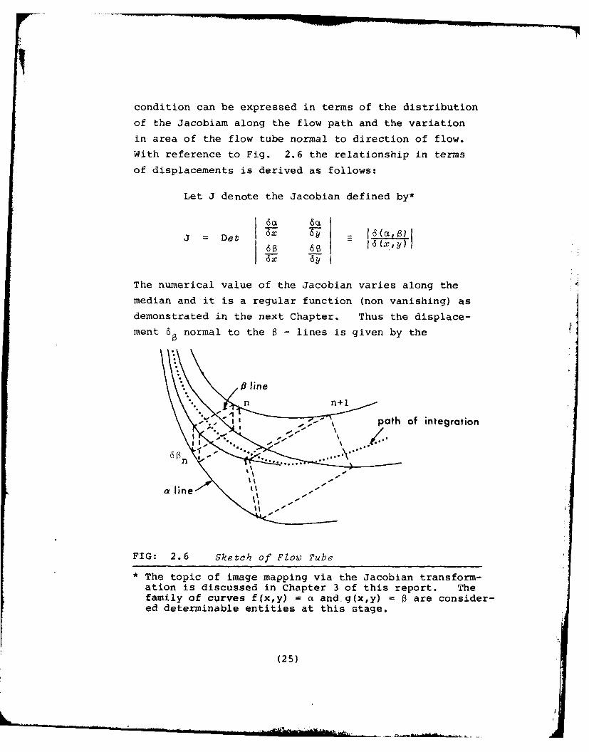
condition can be expressed in terms of the distribution

of the Jacobiam along the flow path and the variation

in area of the flow tube normal to direction of flow.With reference to Fig. 2.6 the relationship in terms

of displacements is derived as follows:

Let J denote the Jacobian defined by*

6ac 6a~

J = Det 67 =)

The numerical value of the Jacobian varies along the

median and it is a regular function (non vanishing) as

demonstrated in the next Chapter. Thus the displace-ment 6 normal to the 8-lines is given by the

line

, - path of integration

\ ..... . .

line it/ I%

FIG: 2.6 Sketch of Flow Tube

* The topic of image mapping via the Jacobian transform-ation is discussed in Chapter 3 of this report. Thefamily of curves f(x,y) = a and.g(x,y) 8 are consider-ed determinable entities at this stage.

(25)

expression

n.A n .6n j n+l An+l.6 n+l

whence

J .A= n n 6 .i66J A n. 21

n+ n+ n+l 2.10

The displacement of the centroid of a cell 6s is given

by the linear approximation:6 s = (6 n + 66+) 2.11

n 2 n n+l

where the notation is that shown in Fig. 2.6. On the

boundary the displacement in a given interval of time

due to surface traction reduces 6 to 6 if we take

the first cell as a line element

i.e. n = 1 6h 6S

where 6s is deduced from the velocity as given by

Equation 2.6. The Equations 2.10 and 2.11 enable

tracking the values of displacements from the source

of boundary perturbation to a terminal point on the

boundary i.e. the exit of the material from the net.

To calculate the displacement it is necessary to have

an expression for the cross sectional area of the flow

tube at stations along the flow path. The relation-

ships of the theory of curvilinear coordinates provide

a general expression for the area, Marsden and Tromba

(1975). pp 314.

viz. Az) = 2 + 6(Xz) + 16(cz 2 dx dyfD 16(y,z) 16(x,z) dxy

where Az) denotes the area at any section 2.12

(26)

2.5 Synthesis of Theoretical Formulations

The foregoing analysis involved the hypothesis that

the rate of flow can be related to the gradient of

mean normal stress a priori. The mean normal stresses

are considered spatially invariant with time and

those values determined by linear elastic theory for

constant boundary conditions. The notions of

similitude and cross-correlation were applied to yield

a dimensionally consistant relationship, i.e. equation

2.6. In order to establish a connection between the

author's approach and orthodox analysis of flow problems,

the governing differential equations for viscous flow

is invoked. These classical equations collectively

known as the Navier-Stokes equations are basic to

analysis to both Newtonian and non-ideal fluids.

The Navier-Stokes equation for two-dimensional steady

flow of an incompressible fluid with constant coefficient

of viscosity q and densityP reads:

p(- u 6 ( 2 + --) = oP(6U + _ + J-)+ (. L +-fU6x 2 6y 2

+ v +6u +( 2L + 62v)

6( 6+ 6+ - ) 6x2 6y2

2.13(a)

Where u and v are the velocity components in the

xy coordinate directions and p is the mean fluid

pressure at a point (not a hydrostatic pressure)

Chang Lu (1973). Equation 2.13(a) together with the

continuity equation completes the classical formulation.

(27)

In the two-dimensional region the continuity equation

is given by the expression:

6u 6v6X 6

Negiicting acceleration but including inertial terms

we have the expressions

6u oy- 066)u 6 2 u = + _U6,p(u,, + Vv) - np+-- -

6X 2 6y 2 6y

Under a coordinate transformation to another orthogonal

frame of reference the property of invariance enables

writing the equation 2.13(b) for the a, coordinates

in the form:

6u _6. u t2) -_£.G,.,, - + V6 - n +-- =6 a2 6

2 a

6v 62v 62v

y(u - + V- - + - - 2.13(c)6C(2 682 66

where now u and v are referred to the orthogonal spatial

coordinates of the a,6 net, and the term 6 is known

from a separate analysis of the stress field.

The first equation of the set 2.13(c) only need be

considered because the mean pressure gradient is zero

everywhere within the solution domain for the right

hand side of the second equation, i.e.

(28)

FQ

6P

Furthermore 0 therefore 6u v = 06b 5B2

Thus the equation 2.13(c) reduces to an ordinary

differential equation with respect to the a - lines,

viz.d2u _ du

U = 2.13(d)dCL 2 Pda F

writing the equation in the form

id 2u _ 1 U_2

da 2 .tF

and integrating we obtain the Riccati differential

equation

du 1n Tl- : - P ( a ) = C 2.13(e)1

This nonlinear and non-homogeneous ordinary different-

ial equation can be solved for u if a particular

solution can be deduced, Courant and John (1974)Hidlebrand (1957). The general solution is formed

from the known function by exponentiation and the

ordinary process of integration with one arbitrary

constant as given in Courant 1974. It appears that

such solutions are mainly relevant in fluid mechanics

or aravitational flow problems i.e. problems where

the driving forces are derived from the gravitational

influence on the mass density. However, it is

significant to note that the displacements will have

similar distributions whether equations 2.11 or 2.13(e)

(29)

~~~~~~~~~. .L, ' ._ ... .., .* .' .. ..%

are used. Finally the equation 2.13(e) has as its

domain of independent variable a the path of integration

inscribed on the physical flow line which is the same

median path as that proposed for evaluating the

correlation function G{ao} of equation 2.7.

(

(30)

I. --

CHAPTER 3

MAPPING FUNCTIONS FOR ORTHOGONAL NETS

, a

3.i .'t,)w uets: AV1'rox1rizat4on 2by Po7.yuom a zs

In this chapter a method for the functional representation

of the geometry of orthogonal trajectories is presented.

Families of orthogonal trajectories are encountered in

hydraulic flow nets, electrostatics and stress fields,

or indeed any physical problem described by Laplace's

Equation. Flow nets are conventionally derived from the

theory of complex variables in an exact formulation,

approximated by the finite difference and finite

elements techniques, or simply sketched freehand to match

a particular set of boundary conditions. The generating

functions deduced from complex variable theory can be

quite complicated, while no functional representation

emerges from the alternative methods. The problem as

posed herein is to fit simple expressions which adequately

describe the geometry in functional relationships.

The method proposed is that of trial fitting of poly-

nomials where the selected polynomials consist of a set of

harmonic mapping functions. These functions are

generated from the definition of a complex function viz.

f(x,y) = (x + iy)n : n = 1,2,3 ...; i = /

Thus by taking values of n to order 4 we obtain harmonic

functions which are deemed to approximate the geometry of

an orthogonal net. Letting 0 and ' represent the co-

ordinates of a mapping function in a Cartesian frame of

reference then the geometry is described by the

relations:

(31)

= A(2x+y) + B(x 2 -y 2 ) + C(X 3 -3xy 2 ) + D(x +y4 -6x 2 y 2 ) +

A(2y-x) + B(2xy) + C(3x 2y-y 3) + D(4x3y-4y3 x) + Io

(3.1)

where A, B, C, D are scaling factors (real numbers).

The functions ( ,y), i (x,y) map a rectangular mesh into

a distorted shape where the lines x = cl, y = c2 in the

(x,y) plane appear as orthogonal trajectories in the

(4,p) space irrespective of the values of the sealing

factors or the constants c1 , c2. Now suppose that a

plot of 0 versus q) in Cartesian coordinates is available

from some source problem in electrostatics or

ground water seepage. The task is to

firstly find the origin of the generating functions

0 (x,y), i (x,y) if in fact the plot stems from a single

origin, and second to extract the expressions that express

the geometrical pattern in algebraic form. Assuming

then that the net can be traced to a single origin, i.e.

not bipolar or multipolar coordinate systems, the proposed

analysis proceeds as follows:

1. A cell in (0,i) space bounded by four intersecting

trajectories is selected (remote from the confluence

of lines that indicate a possible location of this

origin of the coordinate system).

2. Simultaneous equations are written for the selected

order of the harmonic functions by taking the nodes

in turn with one of the four corner nodes as a

temporary origin.

3. The set of simuitaneous equations is solved for the

(32)

unknown values of the constants as given in Eqn. (3.1).

4. A search for those values of the constants which are

consistent with the constraint that the coordinate

intervals of (x,y) are restricted to integers is

implemented.

5. The global origin with respect to the temporary origin

is located by referring back to the results of the

search of step 4 above.

Even in the case of a bipolar net the method can yield the

functional relationships (at least locally) and it also

may be applied to freehand plots in a piecewise scan of

the net cells. Even freehand plots lead to well con-

ditioned equations i.e. small changes in , values

are not grossly reflected in the values of the scaling

factors.

The algebra can be considerably reduced by eliminating

biquadratic terms, i.e. letting D = 0; this is a

simplification that is well justified because of the

ability of cubics to produce the optimum fit to an

arbitrary continuous function (c.f. the theory of splines

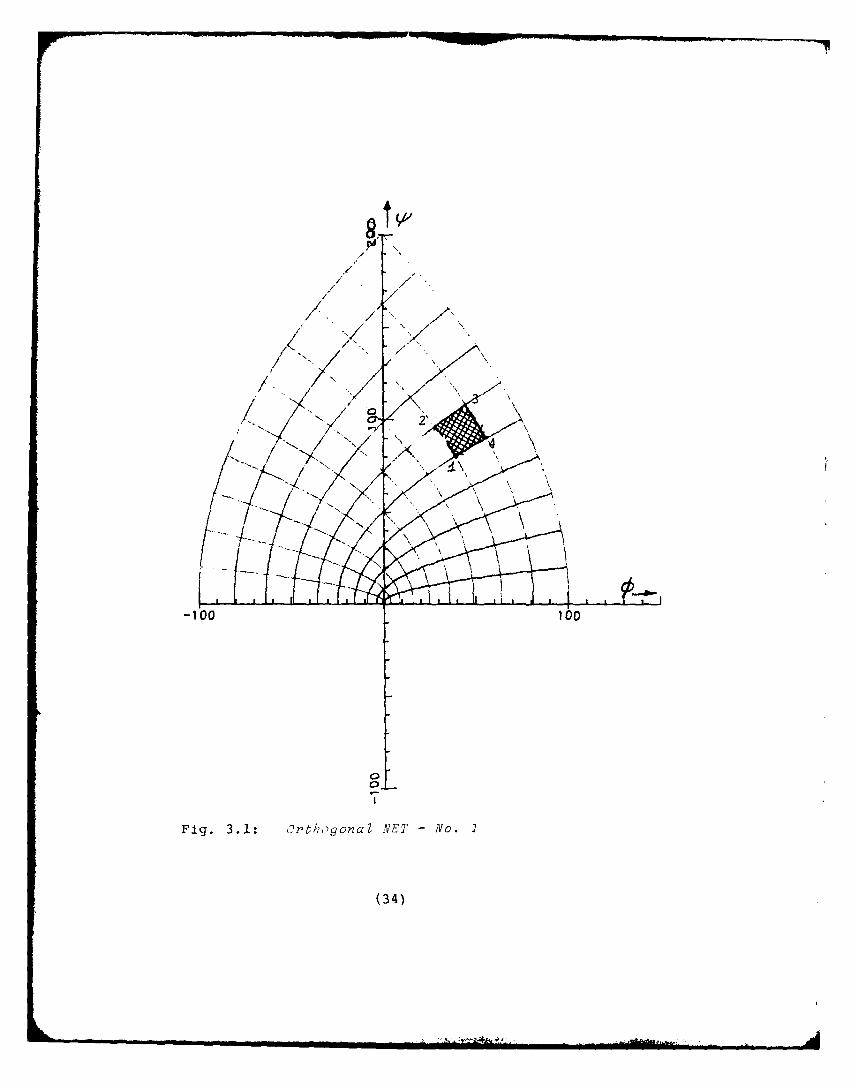
in succeeding chapter). Consider the plot of two

functions 0 and i in Cartesian coordinates as shown in

Fig. 3.]. If we isolate any cell and select a

temporary origin e.g. cell and the node marked 1 of inset

in Fig. 3.1 we can write the coordinates of the nodes

as"Node 1 (Xo, yo)

2 (Xo' Yo + 1)

3 (x0 + 1, YO + 1)

4 (x0 + 1, y0 )

(33)

14~

-100Qt00

Fig. 3.1: Orthogonal NET -No. 2

(34)

where (x0 ,y0 ) are the specific Cartesian coordinates of

the lower left hand node of the cell.

Substituting these ordered pairs in Equation (3.1) for

the abbreviated cubic version we obtain the following:

Node 1

= A(2x0+yo ) + B(X2 -Y2 ) + C(X 3o- 3xoY 20 ) + 0

1 = A(2yo-x0 ) + B(2xoYo) + C(3X 2oY0 -Y 30 ) + o

Node 2= A(2xo+y +1)+B(x 2-y2-2y -1)+C(xo-3x Y2-

2 00 0 0 0 0 06xy 0 -3x ) + 4o

= A(2y -X +2)+B(2x +2x y )+C(x 2 +3x y--2 0 0 0 0 0 0 0 0

Y2-3 y 2 -3y 1) (3.2)

and similarly for nodes 3 and 4. Knowing the values of

4 and i at the nodes we can take any three of the above

equations and solve for the constants A, B, C over a

range of integer values of xoy O. It transpires that

if there ip a unique set of values of the constants that

satisfy all combinations of the equations for the nodal

*,' values throughout the net then a global origin exists

for the particular net. The temporary origin at the

unique values of xoy o gives the clue to the location of

global origin. The offsets are then 0o and o in Equation 3.2.

Before a numerical example is presented it is worthwhile

to take a look at closed mathematical solutions of the

problem of inverting images. With the assistance of a

mathematician, the author arrived at a specimen solution

(35)

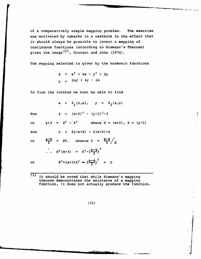
of a comparatively simple mapping problem. The exercise

was motivated by remarks in a textbook to the effect that

it should always be possible to invert a mapping of

continuous functions (according to Riemann's Theorem)

given the image ( ) , Courant and John (1974).

The mapping selected is given by the harmonic functions

* = x2 + 4x - y 2 + 2y

2xy + 4y - 2x

To find the inverse we must be able to find

x = f1 ( ,'), y = f24(,P)

Now = (x+2) 2 - (y-l) 2 -3

or 0+3 = y2 where X - (x+2), Y = (y-l)

and = 2y(x+2) - 2(x+2)+4

or 2 = XY. whence Y =X

X2 (0+3) = X - 2 4)

or _(*+3) ( )~= 0

(1) It should be noted that while Riemann's mappingtheorem demonstrates the existance of a mappingfunction, it does not actually produce the function.

(36)

I

*+3 + /(0+W+ (-4}2

X = 2- (x+2) 22

10+3 + I(+ 3 )2+ 1 -41 2

X= ./-2 = f

2

2 X, +1 f 2 (,1) 3.3(b) Q.E.D.2X(4 2p

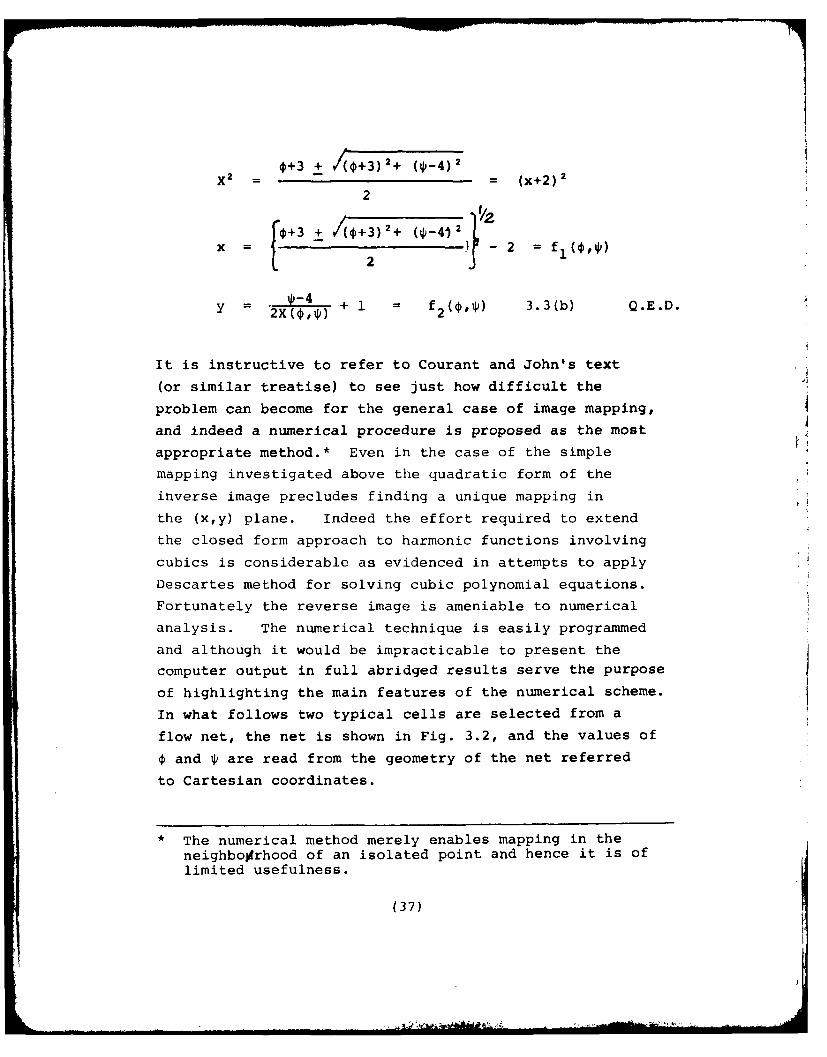
It is instructive to refer to Courant and John's text

(or similar treatise) to see just how difficult the

problem can become for the general case of image mapping,

and indeed a numerical procedure is proposed as the most

appropriate method.* Even in the case of the simple

mapping investigated above the quadratic form of the

inverse image precludes finding a unique mapping in

the (x,y) plane. Indeed the effort required to extend

the closed form approach to harmonic functions involving

cubics is considerable as evidenced in attempts to apply

Descartes method for solving cubic polynomial equations.

Fortunately the reverse image is ameniable to numerical

analysis. The numerical technique is easily programmed

and although it would be impracticable to present the

computer output in full abridged results serve the purpose

of highlighting the main features of the numerical scheme.

In what follows two typical cells are selected from a

flow net, the net is shown in Fig. 3.2, and the values of

and * are read from the geometry of the net referred

to Cartesian coordinates.

* The numerical method merely enables mapping in theneighbolrhood of an isolated point and hence it is oflimited usefulness.

(37)

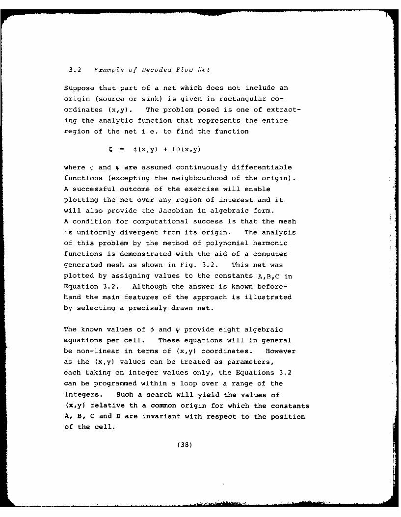
3.2 Example of Decoded Flow Net

Suppose that part of a net which does not include an

origin (source or sink) is given in rectangular co-

ordinates (x,y). The problem posed is one of extract-

ing the analytic function that represents the entire

region of the net i.e. to find the function

= 4(x,Y) + iip(x,y)

where p and d dre assumed continuously differentiable

functions (excepting the neighbourhood of the origin).

A successful outcome of the exercise will enable

plotting the net over any region of interest and itwill also provide the Jacobian in algebraic form.

A condition for computational success is that the mesh

is uniformly divergent from its origin. The analysis

of this problem by the method of polynomial harmonic

functions is demonstrated with the aid of a computer

generated mesh as shown in Fig. 3.2. This net was

plotted by assigning values to the constants A,B,C in

Equation 3.2. Although the answer is known before-

hand the main features of the approach is illustrated

by selecting a precisely drawn net.

The known values of p and ' provide eight algebraicequations per cell. These equations will in general

be non-linear in terms of (x,y) coordinates. However

as the (xy) values can be treated as parameters,

each taking on integer values only, the Equations 3.2

can be programmed within a loop over a range of the

integers. Such a search will yield the values of

(x,y) relative th a common origin for which the constants

A, B, C and D are invariant with respect to the position

of the cell.

(38)

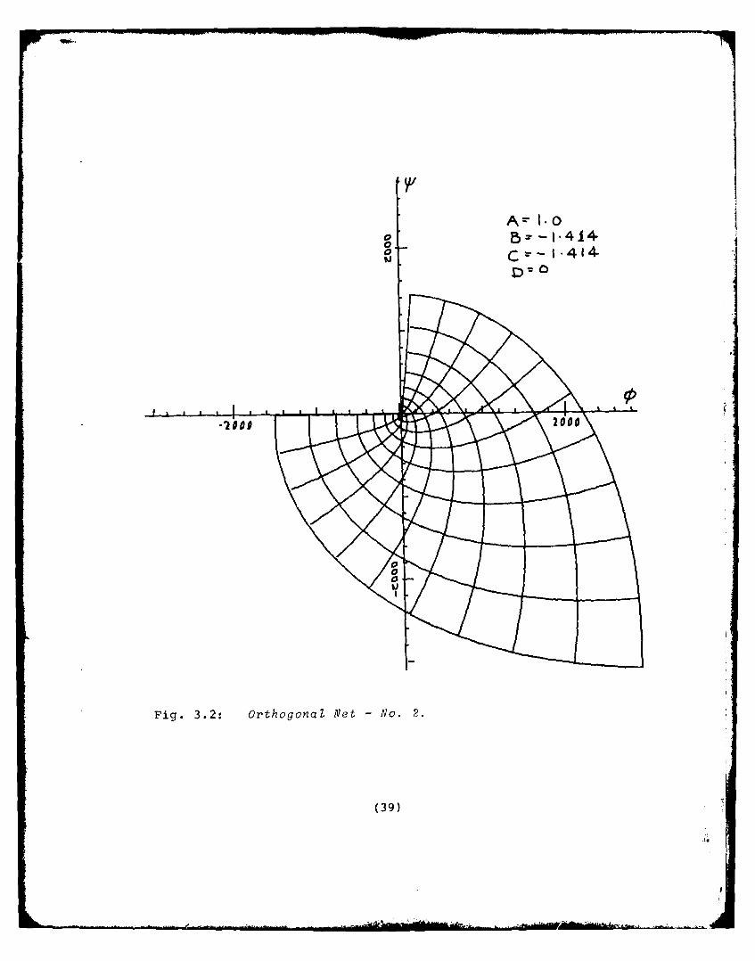
A=- 1.0

Fig. 3.2: Orthogonal Net -No. 2

(39)

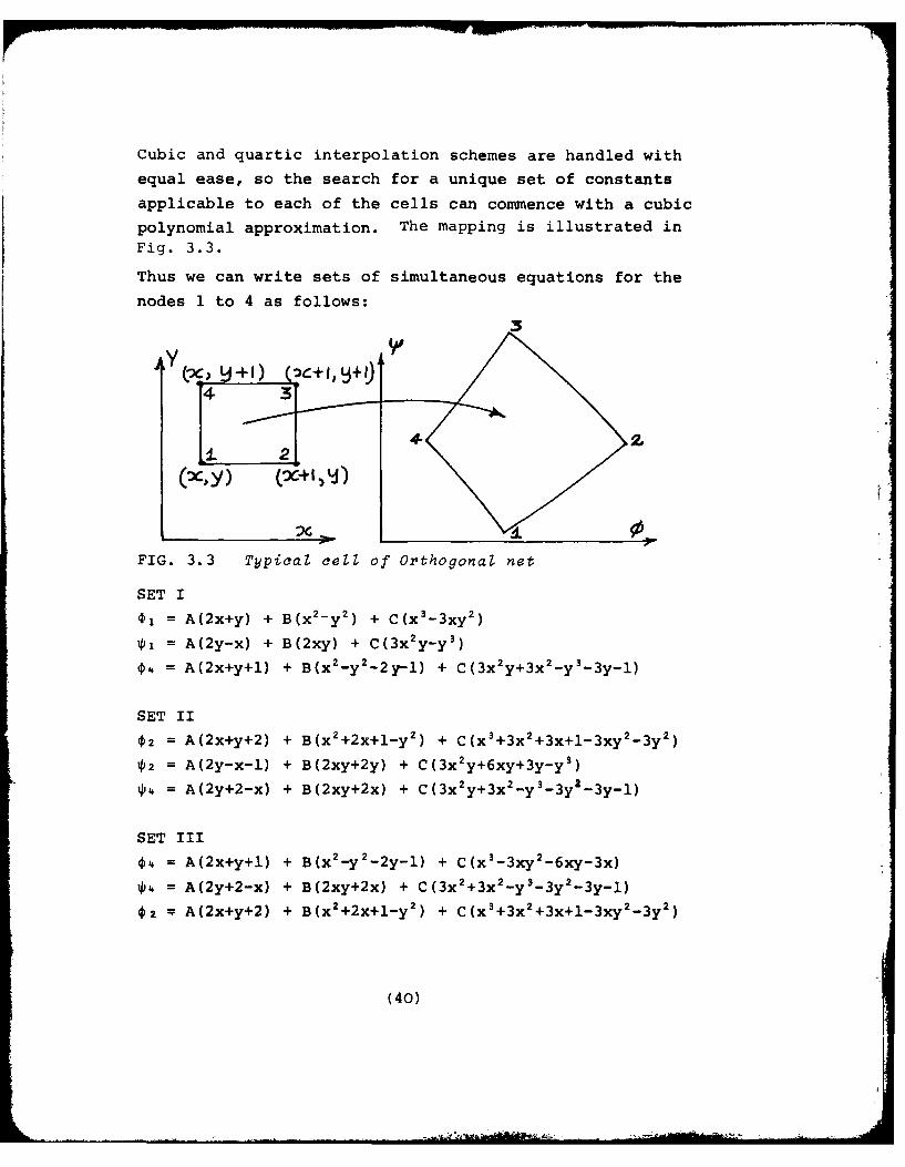
Cubic and quartic interpolation schemes are handled with

equal ease, so the search for a unique set of constants

applicable to each of the cells can commence with a cubic

polynomial approximation. The mapping is illustrated inFig. 3.3.

Thus we can write sets of simultaneous equations for the

nodes 1 to 4 as follows:

FIG. 3.3 Typi~cal cell of Orthogonal net

SET I

D= A(2x+y) + B (X2 y 2 ) + C(x3 -3XY 2)

ik: = A(2y-x) + B(2xy) + C(3x2y-y3)

= A(2x+y+l) + B(x2-y2-2y-l) + C(3X 2 y+3x2_y

3 -3y-1)

SET II

2=A(2x+y+2) + B (X2 +2x+l-y2) + C(X3+3X2 +3x+1-3XY 2 -3y2)

*= A(2y-x-1) + B(2xy+2y) + C(3X 2 y+6xy+3y-y3)4a = A(2y+2-x) + B(2xy+2x) + C(3x2y+3x2-~y3 -3y2 -3y-l)

SET III

4=A(2x+y+l) + B(X2-y2-2y-l) + C(X 3 -3XY 2 -6xy-3x)

= A(2y+2-x) + B(2xy+2x) + C(3X2 +3X 2-y 3-3y2-3y-l)

2 A(2x+y+2) + B(x 2+2x+ l-y2 ) + C(X 3 +3X 2 +3x+1-3Xy 2-3 y 2)

(40)

SET IV

02 = A(2x+y+2) + B(x2+2x+l-y 2) + C(x3 +3x2+3x+1-3x+l-3xy 2-3y2)

01 = A(2x+y) + B(x2-y 2) + C(x 3-3xy 2)

04 = A(2x+y+l) + B(x2-y 2-2y-l) + C(x3 -3xy 2-6xy-3x)

SET V

IP2 = A(2y-x-l) + B(2xy+2y) + C(3x 2y+6xy+3y-y 3)= A(2y-x) + B(2xy) + C(3x 2 y-y 3 )

4 = A(2y+2-x) + B(2xy+2x) + C(3x 2 y+3x 2 -y 3-3y 2 -3y-l)

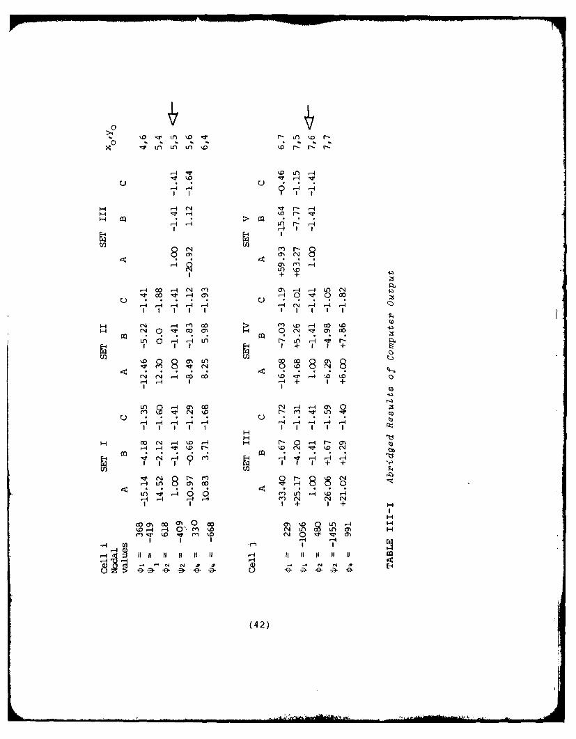
The equations above are solved for the constants A, B and C

by inserting values of 4 and t at the nodes and a range of

integer values for x and y; the process is continued until a

particular pair of x,y values yield the same values for the

constants irrespective of the ordering of the set of equations.

The consistent values are identified in Table ll]-Iby arrows in

right hand margin. Because of re-ordering of node numbers in

programs run on the Hewlett Packard and Digital computers the

diagrams are at some variance with the tabulated results.

Nevertheless, the results as listed, the program in BASIC,

demonstrates the key features of the analysis.

(41)

i.

- LA Ln k- r % r-

x0 LA LA N r Nr r:

.-4 qT '"D LA) r-

U * -!

-4-44-

H0 14 r l -4 1-4 Lr N 4

H- ,-I (1 ' .0 -4 O' %D -H C- 0 * C )C q 7

.- 4 .- L ) N 4 'r

++

110 19 84 ON CL 000 8- -4 LA (C .' .- O1 0 4 1

.- -4 ~4 - 4- N -

Hn ( -4 M WO m .0

m (N r- CO O-I H 0 4 r- M ~CLAO -4: .- A A -

+ +

(N ( .z -A C C'0 Ln ,-4 w. '.-II- M- +N N +

+ +

~ CO ( r-4 '~ r-4-4-

(42

The results, determined for cells i and j, are given in

Table III-I where the constants for a partial list of the

independent parameters are tabulated.

The position of the global origin is at the same location

for the two cells chosen here:

Cell i : origin : x = 5 and y = 5

Cell j : origin : x = 7 and y = 6

Constants A = 1.00, B = -1.41, and C = -1.41, D = 0.

The results can be verified for all cells outside the

immediate vicinity of the origin i.e. where the change is

curvature is moderate. The equation of the entire net are

now established in the relationships

=2x+y-l.41(x2-y2)-l.41(x3-3xy 2 )

= 2y-x-2.82(xy)-l.41(3x 2y-y3 )

and the analytical function 4 is completely defined. The

flow net can be extended indefinitely by using these

functions.

However in stress analysis the relationship is normally

encountered with form ' = f(p). Thus equation 3.3 would

be reduced to:

p = 2X(X 2-4-3) + 4 (X = x+2) 3.-'.c

On a Cartesian plot the expression ' = f(o), for a specific

domain of O(x,y), is a family of curves because * is a

multivalued function if we vary x or y. The curvilinear

plot is more readily described in curvilinear coordinates

wherein the points set (x,y) are regarded as curvilinear

coordinates. From this viewpoint the differential relation-

ship for areas of cells is given by the expression

(43)

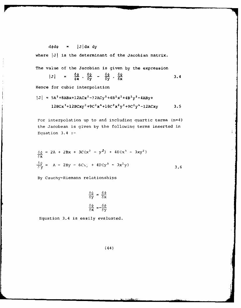
d4~di IJIdx dy

where IJI is the determinant of the Jacobian matrix.

The value of the Jacobian is given by the expression

Iji 6 4 -§ 3.44x *6y 6y *6x

Hence for cubic interpolation

IJI =5A2 +8ABx+12ACX2 -12ACy 2 +4 B 2X2+4B2y2 -4ABy+

12BCX3 +12BCXy2+9C2X4+18C2X2y2+9C2y4 -12ACxy 3.5

For interpolation up to and including cquartic terms (n=4)

the Jacobean is given by the following terms inserted in

Equation 3.4

6 = 2A + 2Bx + 3C (X2 _ y 2 ) + 4D(x3 3 3Xy2 )

-L= A - 2By - 6Cx1 + 4D (y3 - 3 X 2y)3.

By Cauchy-Riemann relationships

6y 6x

65X 6y

Equation 3.4 is easily evaluated.

(44)

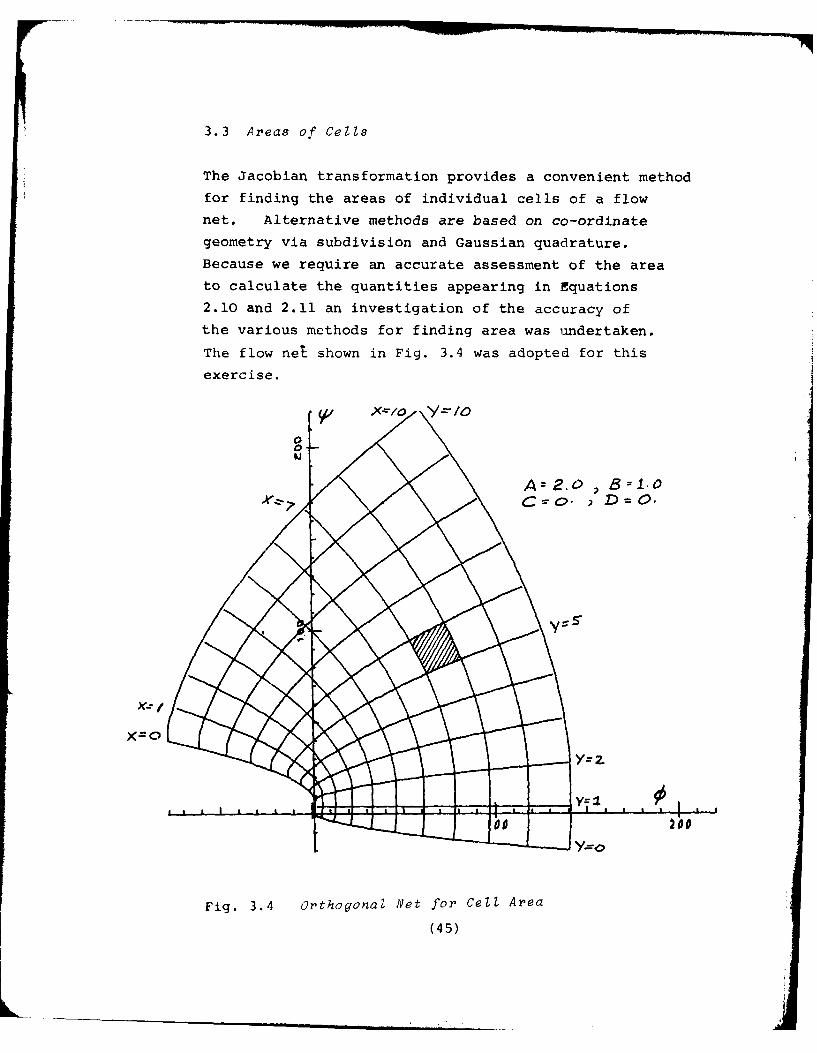
3.3 Areas of Cells

The Jacobian transformation provides a convenient method

for finding the areas of individual cells of a flow

net. Alternative methods are based on co-ordinate

geometry via subdivision and Gaussian quadrature.

Because we require an accurate assessment of the area

to calculate the quantities appearing in Equations

2.10 and 2.11 an investigation of the accuracy of

the various methods for finding area was undertaken.

The flow net shown in Fig. 3.4 was adopted for this

exercise.

A = 2.0

X=O

Y=

Fig. 3.4 Orthogonal Net for Cell Area

(45)

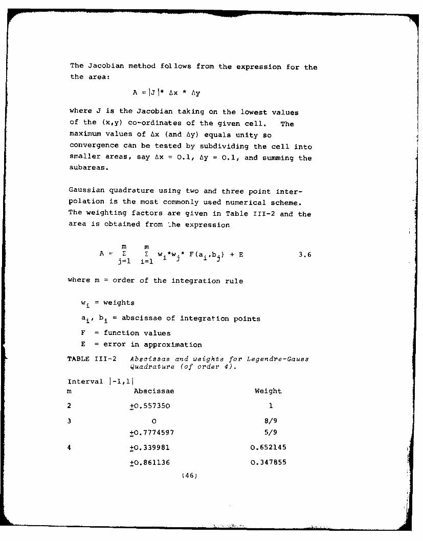
The Jacobian method follows from the expression for the

the area:

A =IJI* Ax * Ay

where J is the Jacobian taking on the lowest values

of the (x,y) co-ordinates of the given cell. The

maximum values of Ax (and Ay) equals unity soconvergence can be tested by subdividing the cell intosmaller areas, say Ax = 0.1, Ay = 0.1, and summing the

subareas.

Gaussian quadrature using two and three point inter-polation is the most commonly used numerical scheme.The weighting factors are given in Table 111-2 and the

area is obtained from 'he expression

m mA E E wi*w.* F(ai,b.) + E 3.6

j=l i=l 1

where m = order of the integration rule

w i = weights

a ,, bi = abscissae of integration points

F = function values

E = error in approximation

TABLE 111-2 Abscissas and weights for Legendre-GaussQuadrature (of order 4).

Interval 1-1,11m Abscissae Weight

2 ±0.557350 1

3 0 8/9

±0.7774597 5/9

4 +0.339981 0.652145

+0.861136 0.347855

(46)

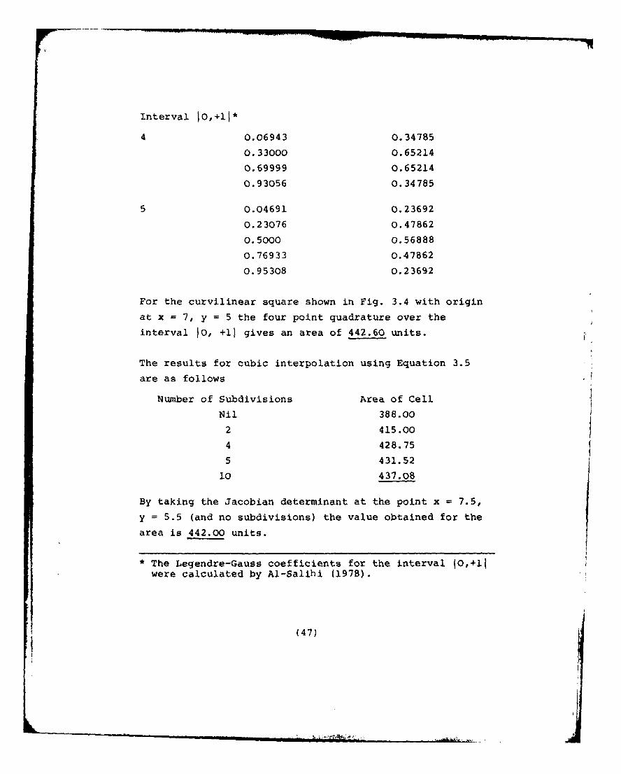
Interval )0,+.lI*

4 0.06943 0.34785

0.33000 0.65214

0.69999 0.65214

0.93056 0.34785

5 0.04691 0.23692

0.23076 0.47862

0.5000 0.56888

0.76933 0.47862

0.95308 0.23692

For the curvilinear square shown in Fig. 3.4 with origin

at x = 7, y = 5 the four point quadrature over the

interval 10, +1) gives an area of 442.60 units.

The results for cubic interpolation using Equation 3.5

are as follows

Number of Subdivisions Area of Cell

Nil 388.00

2 415.00

4 428.75

5 431.52

10 437.08

By taking the Jacobian determinant at the point x = 7.5,

y = 5.5 (and no subdivisions) the value obtained for the

area is 442.00 units.

* The Legendre-Gauss coefficients for the interval (0,+11were calculated by Al-Salihi (1978).

(47)

I. .. . . .. .... . , 4 . _. . .... -

Hence it appears from the quantities underlined in above

that the Jacobian determinant evaluated at the intersection

of the medians to the sides gives a good estimate for the

asymptotic value of the area projected by subdividing the

cell. Where the Jacobian can be determined analytically

it proves more expeditious than quadrature formulae which

in itself is a motivation for trying to fit polynomials

to flow nets.

3.4 The Conjugate Function

The foregoing theory pertains to conformal mapping from

one plane to another. At this juncture it is relevant

to compare the geometrical exercise with its physical

counterparts, namely, the derivation of velocity potential

and stream functions in fluid mechanics, or the plotting

of equipotential and flow lines in electrostatics and

soil mechanics. In these problems it often transpires

that one of the functions is more readily plotted than

the other on physical grounds. For instance as an

example of a potential function let the distribution of

the potential be denoted by p (which is analo-ous to the

previous interpretation of c as a curve in the plane of

Cartesian space) where 0 is a known function of position

in the solution domain in the x-y plane. In this

instance 0 represents the distribution of a potential

such as pore pressure, voltage or magnetic flux. Take

for example the real part of the harmonic function

= x2 + 4x - y 2 + 2y

where * satisfied Laplace's equation,Sh+6_=0

6x2 6y2

(48)

The conjugate function must satisfy

6_ 6_h = 06x2 6y2

The function 4 is deduced from the expression

f = y f dy. - f (,,) dx 3.6YO 6 x

Xo Y=Yo

In this example

4) = 2 S (x+2)dy + 2 1(y-l) y=yo dx

= 4y - 2x + 2xy + c

where c = 2(xo - xoyO - 2yo)

Thusly the real and imaginary parts of an analytic

function are evaluated. However, this simple example

merely serves to demonstrate the method of conjugate

functions; in practical examples the process can become

very difficult. A general method using finite difference

approximations on a curvilinear orthogonal grid combined

with an analytic solution has been reported by Centurioni

and Viviani (1975).

The discource in this Chapter leads to the conclusion

that mapping functions can be deduced by inspection of

the constraints in a problem. The initial trials

can be adjusted to approximate flow paths in the

(49)

areas of fluid and soil mechanics, diffusion process

and electrostatics. Experience of generating

orthogonal nets by simply varying the parameters in a

cubic polynomial representation suggests that a useful

technique has been introduced. By using the computer

generated plots to overlay a given potential field the

functional relationships can be determined piecewise, or

in favourable circumstances the mathematical description

of the entire field.

We have performed these exercises on a variety of flow

nets with the result that it has always been found

possible to locate the origin if the net had been

accurately drawn from a single origin. The values

listed in Table III-I indicate that the sets are distinct,

leading to well conditioned simultaneous equations. The

main drawback to this approach is the stipulation of a

unique origin of the net. It will be seen in the

further development of our analysis that this requirement

can be relaxed albeit at the expense of computational

effort. A further drawback is due to the fact that theconjugate function T is not an even function, as may be

seen by inspection of Equation 3.1. Therefore it results

in plots with skew symmetry which limits class of problems

to which the nets may be applied. The only symmetric plot

results from the quadratic terms of Equation 3.1.

Negative integers employed as the exponents in the analytic

function lead to cumbersome algebra in the Jacobian determinant,

and hence taking n < 0 confers no practical advantage.

(50)

CHAPTER 4

CUBIC INTERPOLATORY SPLINES

4.1 Introduction

The theory of splines is well documented so only a brief

review is presented herein as a background to the develop-

ment of a computer program for parametric cubic spline

interpolation of material flow paths.

Splines are an important tool in modern numerical analysis

for

1) Interpolation

2) Numerical integration and differentiation

3) Numerical solutions of ordinary differential

equations

4) Numerical solutions of partial differential

equations.

However the interpolatory property of the splines is only

of interest here. The great advantage of splines in

interpolation is that they do not have the oscillatory

property of the interpolating polynomial. The most

widely used splines are the cubic splines.

4.2 Definition of a Cubic Spline

A cubic spline S(t) with modes tit t2 ..... tn

(ti < t2 < t3 . . . . . < tn) is a function which in theinterval ti $ t < ti + 1 (i = 1,2, ... n-l) reduced to a

cubic polynomial in t, and at each interior node t

(i = 2,2,...n-1), S(t), S'(t) and S'(t) are continuous

function and its derivatives.

(51)

Such a function may be represented in the interval

t < t < t + 1 (i = 1,2,...n-l) in the form

S = F(t) = ai t 3 + b it2 + cit + di

where, associated with each cubic arc Si, there are four

unknown coefficients ai, bi, ci and di. It follows that

there are 4 (n-i) conditions to be fulfilled, so that S(t)

is fully defined mathematically

1) S(t) must match at the interval nodes

S(ti) = T(ti)i.e. n equations

2) S(t) must be continuous over the boundaries

S(t_) = S(ti+) i = 2(1)n-1

i.e. n-2 equations

3) S'(t) and S''(t) must be continuous over the

boundaries

S'(t) = S'(ti+)

S''(ti) = S''(ti+) i = 2(1)n-1

i.e. 2n-4 equations

Hence there are 4n-6 equations with 4n-4 unknowns. To

overcome this problem the natural cubic spline can be

employed which has the extra condition for the second

derivatives

4) S''(t1 ) = 0

S''(tn) = 0

This corresponds to letting the physical spline project

past the end weights. Usually one is not interested in

t < ti or t > tn but if they arise the natural spline is

(52)

I!

extended by straight lines agreeing in value and slope

at the ends ti and tn.

The second derivative is then also continuous at the ends.

Hence there are two more equations to deduce 4n-4 equations

to solve for 4n-4 unknowns. Thus the mathematical spline

is explicitely defined.

Condition (1) implies that the curve goes through the knots,

or nodes. Conditions (2) and (3) imply continuity of

alignment, continuity of slope and continuity of

curvature respectively.

In contrast to polynomial interpolation which increases the

degree to interpolate more points, here the degree is fixed

and one uses more polynomials instead - one for each

interval. For each interval the natural cubic spline is

unique and is the smoothest interpolating curve through

these points.

4.3 Derivation of the Natural Cubic Spline

For notational convenience let

hi = ti+ 1 - ti

S i(t) = s(t), tcjti,ti1l

M = S''(ti)

Because Si(t) is a cubic polynomial the second derivative

Sj'(t) is a linear polynomial and can be expressed in the

form

(53)

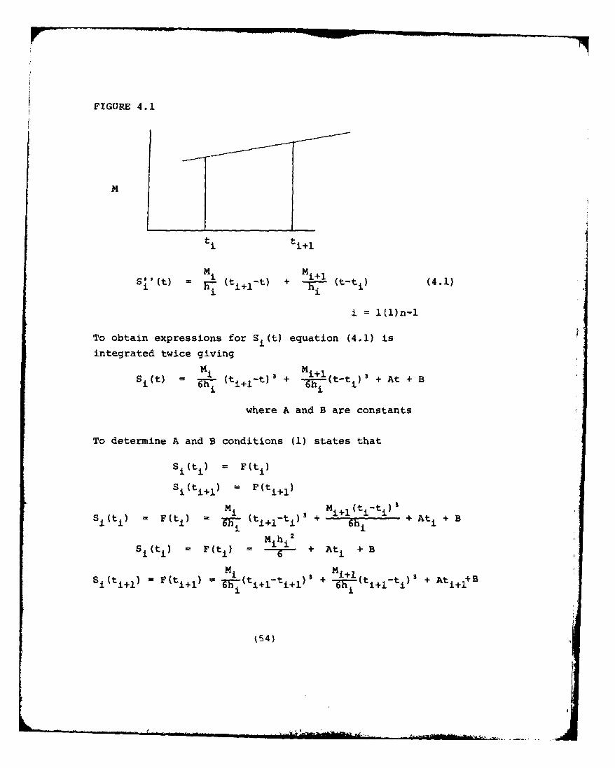
FIGURE 4.1

ti

MM

i i

i = 1(1)n-i

To obtain expressions for S (t) equation (4.1) is

integrated twice giving

14 MS (t) =(t W

+ -i -i(tt)3 + At + BSi~ -6h~ 'i+i7' 6h

where A and B are constants

To determine A and B conditions (1) states that

Si(ti) = F(ti)

Si (ti+) = F(ti+I )

M tFt i (Mi+ (i-t i )Si (t i ) F(t i ) = i (ti+l-ti) t + 6h + Ati + B

Si(ti) = F(ti) = m + Ati + BM i+- ,+1

iti+ Fti+ h(ti+l-ti+ 1 ) ' + W i+l-i, +Ati+ s

054)

or M h 2Mi-1h1

Si(ti+) = F(ti+l) = 6 + i+l

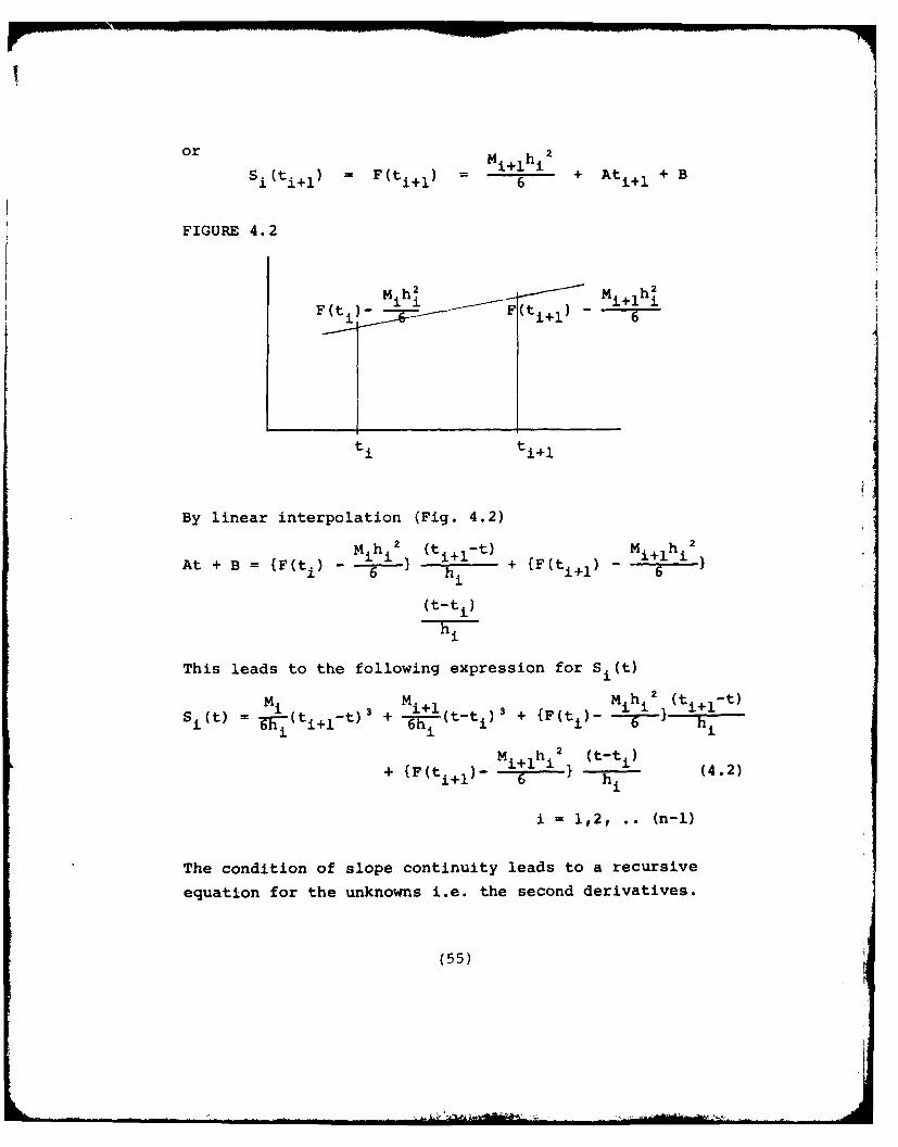
FIGURE 4.2

(t ii i+l iF _t (t i+l) 6

ti ti+ 1

By linear interpolation (Fig. 4.2)

Mih 1 2 (ti+l-t) Mi+lhi 2

At + B = {F(t i ) - --gt-} h + {F(ti+l) 6

(t-ti)

This leads to the following expression for Si(t)

S i + t) M3h+ 2 (ti4 l-t)i(t ) =W 7 + -) h

+ {F(ti M)- 6 h i (t-t1) (4.2)1+1hi

1 1,2, .. (n-1)

The condition of slope continuity leads to a recursive

equation for the unknowns i.e. the second derivatives.

(55)

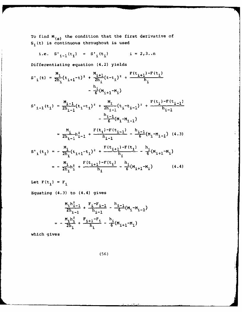
To find M the condition that the first derivative of(s)Si(t) is continuous throughout is used

i.e. S'iil(ti) = Sti(ti) i = 2,3..n

Differentiating equation (4.2) yields

Mi Mi~ ' F (t ) -F (t )

s' i (t) = . (ti it) 2 + mi (t-ti)2 + hi

h.- 4Mi -Mi)

M Mi F(t.)-F(tS' t = (titi)2 + 2- (ti-ti ,) Z + hi 1

i-h i-i (- )

- 1h 2 +i-i1-i-i + hi_ 1 - --- Mi-Mi_) (4.3)

Mi F(ti+I )-F (t) h is i - iti+-i + h- -(Mi+(-Mi)

- ( m 2 F (ti+ )F(t i ) h i2h i + hi 6 - +-Mi) (4.4)

Let F(ti) F i

Equating (4.3) to (4.4) gives

Mih - + Fi-Fi- hi_

2hi 1 hi- 1

M h2 F -2= i h i 6 Mi+l-)i i iFi h

which gives

(56)

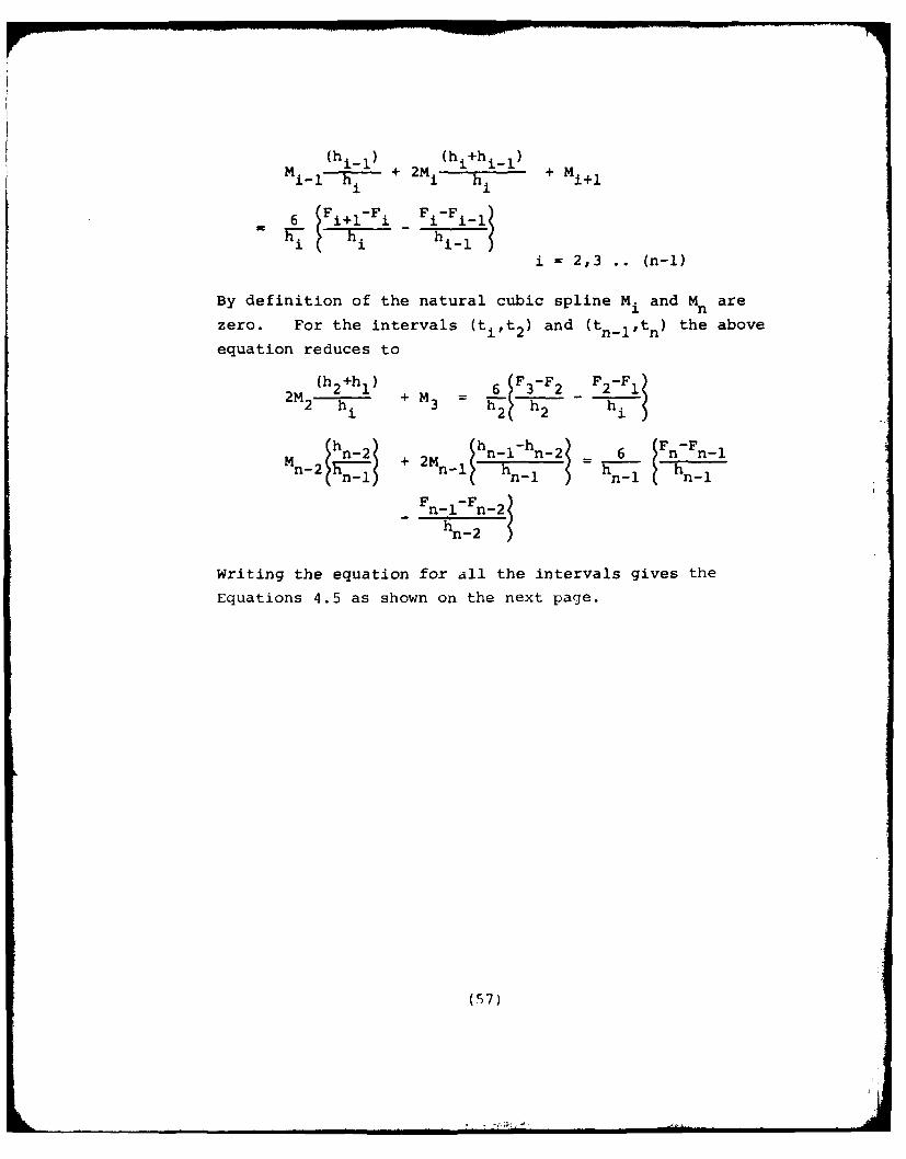
(hi_-1 ) (hi +hi1- )M + 2Mi h + Mi+l

6 Fi+l-Fi Fi-Fi-i

i = 2,3 .. (n-I)

By definition of the natural cubic spline Mi and Mn are

zero. For the intervals (tit 2 ) and (tn-ltn) the above

equation reduces to

(h 2 +h 1 ) 6 (F 3-F 2 F2-F 12M2 hi + M3 = h2h 2 h i _

m ln-2 + 2M hn-l-h n-2 6 IFn-F n-Ms-21 n n'h_ , -l n' -- l

F n-l-F n-2h- n-2Shn-2 i

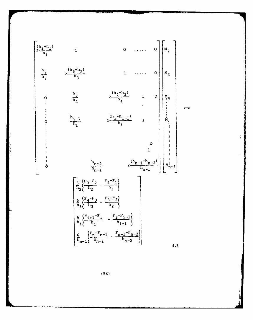
Writing the equation for all the intervals gives the

Equations 4.5 as shown on the next page.

(57)

(h 2 +h I ) 201 ..... 0 M 2

h 2 (h 3 +h 2 )

F3 h3

h (h 4 +h 3 )

h3 43

0 4

h 2 (hi+hi-1 ) M

h 2 h~ 3

0I

-I

6 (F 3 -F 2 F 2 -F 1 )hi

6 (F 4 -F 3 F3 -F 2 j

1 --

h hn~ .. hn_ 2-

L4-

________ Fi-Fi 1 )

6 -F 1 ..

6 IFn-F n-1 Fn-l-F n-2'

F n-l h han 2L -4.5

(58)

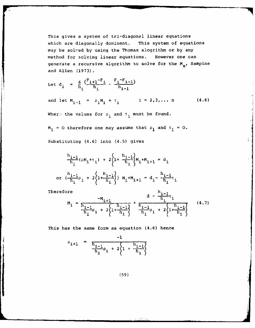
This gives a system of tri-diagonal linear equations

which are diagonally dominent. This system of equations

may be solved by using the Thomas alogrithm or by any

method for solving linear equations. However one can

generate a recursive algorithm to solve for the Ms, Sampine

and Allen (1973).

(Fi+-Fi Fi-Fi-1)Let dh h

i i i-1

and let M = pMi + T i = 2,3,..b n (4.6)

Wher2. the values for 0i and Ti must be found.

M= 0 therefore one may assume that P1 and T, 0.

Substituting (4.6) into (4.5) gives

h.(PMi+ i -) + 2 + h. i i+= di

1 ~h 1 i1

orfh i-i h-- } = + d - --~lTh. 1 n i i i+ . i hi i

Therefore hi_ 1d -K--r i

M = 1+1 +h 1 (4.7)

1R p + 21 i+2l

This has the same form as equation (4.6) hence

~i+1 hi- p + 2 1 +

(59)

---- . .. . o_

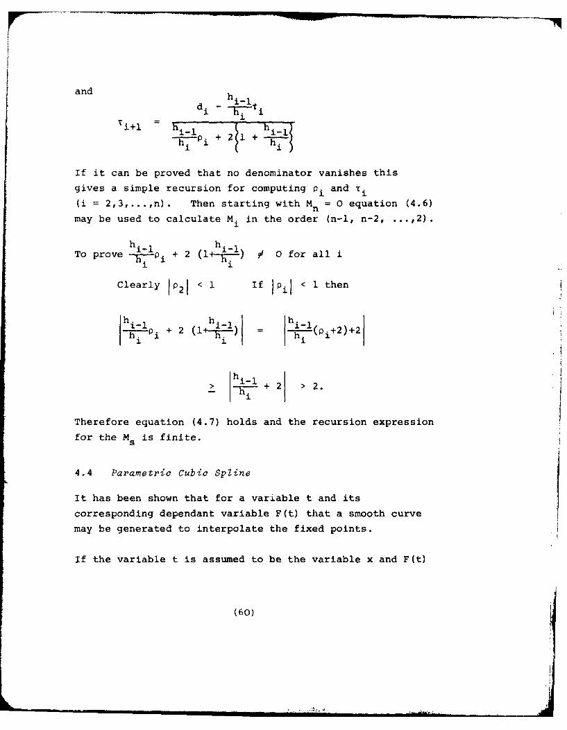
and hi l

di - ii+l h i_ 1 21 hi-li

h i +

If it can be proved that no denominator vanishes this

gives a simple recursion for computing pi and Ti

(i = 2,3,...,n). Then starting with Mn = 0 equation (4.6)

may be used to calculate M i in the order (n-i, n-2, ...,2).

h i-i -To prove --7--Pi + 2 (1 i ) 0 for all i

"i 1

Clearly 121 < 1 If Ipi4 < 1 then

hi-i+ 2 (1-~.-- = h.(pi+2)+2

1 Pi + 1

hi + 2 > 2.

Therefore equation (4.7) holds and the recursion expression

for the M is finite.

4.4 Parametric Cubic Spline

It has been shown that for a variable t and its

corresponding dependant variable F(t) that a smooth curve

may be generated to interpolate the fixed points.

If the variable t is assumed to be the variable x and F(t)

(60)

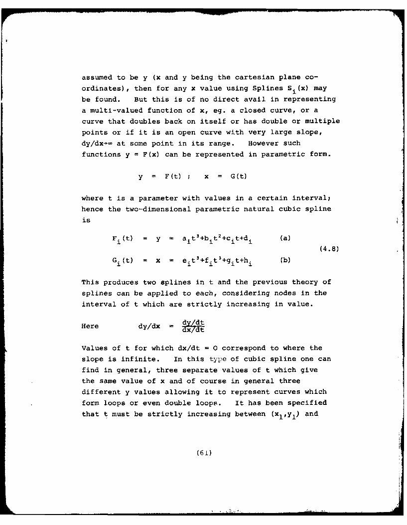
assumed to be y (x and y being the cartesian plane co-

ordinates), then for any x value using Splines Si(x) may

be found. But this is of no direct avail in representing

a multi-valued function of x, eg. a closed curve, or a

curve that doubles back on itself or has double or multiple

points or if it is an open curve with very large slope,

dy/dx-o at some point in its range. However such

functions y = F(x) can be represented in parametric form.

y = F(t) ; x = G(t)

where t is a parameter with values in a certain interval;

hence the two-dimensional parametric natural cubic spline

is

F (t) = y = ait 3 +bi t 2+cit+di (a)

(4.8)

G (t) = x = eit 3+fit 3 +git+hi (b)

This produces two splines in t and the previous theory of

splines can be applied to each, considering nodes in the

interval of t which are strictly increasing in value.

Here dy/dx =dy/dt7dx/dt

Values of t for which dx/dt = 0 correspond to where the

slope is infinite. In this type of cubic spline one can

find in general, three separate values of t which give

the same value of x and of course in general three

different y values allowing it to represent curves which

form loops or even double loops. It has been specified

that t must be strictly increasing between (xly) and

(61)

xn,yn), that is, on the curve in the x, y plane if t takes

the value Ti at the point (xi,Yi ) and taken the value t

at the point (x,y) and takes the value Ti+1 at the point

(xi+l,Yi+I ) then Ti < Ti+I. This means that in the (t,x)

plane and (t,y) plane x and y are single valued functions

of t. If this parameter t is considered as the distance

along the curve then the resulting cubics in t, for x and

y give the curve in the (x,y) plane of that formed by the

spline. If t is the distance from the point (x,Y I ) to

the point (x,y) on the spline along the spline then the

spline may be represented by equations (4.8) (a) and (b).

The values Ti at the point (xi,Yi ) are not known and must

be estimated.

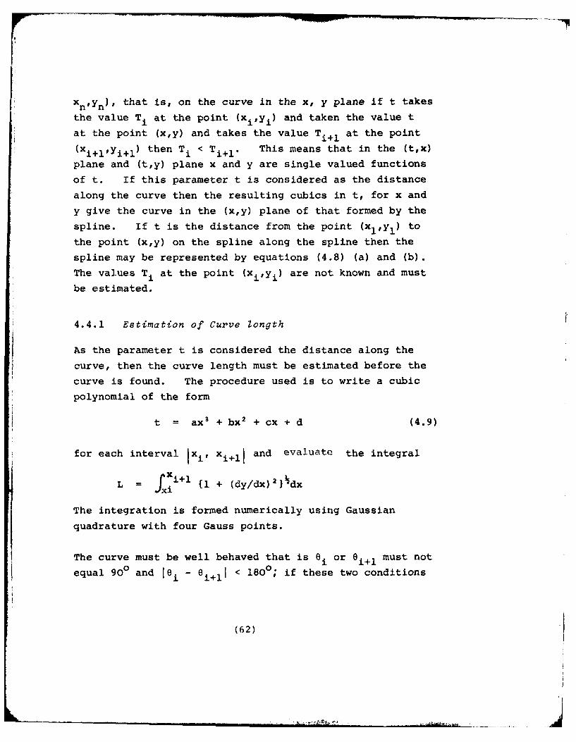
4.4.1 Estimation of Curve longth

As the parameter t is considered the distance along the

curve, then the curve length must be estimated before the

curve is found. The procedure used is to write a cubic

polynomial of the form

t = ax 3 + bx2 + cx + d (4.9)

for each interval lxi, xil and evaluate the integral

L = Xil {1 + (dy/dx)2}dx

The integration is formed numerically using Gaussian

quadrature with four Gauss points.

The curve must be well behaved that is i or Oi+ 1 must not

equal 900 and 16 - 6i+1i < 1800; if these two conditions

(62)

are not satisfied the line must be rotated towards the

horizontal before integration.

The resulting lengths for each interval are added to give

the length of the whole curve. Obviously as this is an

estimated length, the error accumulates as the curve length

increases. When the spline is found using these estimated

lengths, the lengths are re-calculated and by an iterative

process an improved curve length may be found hence giving

a better fit to the locus of the knots.

4.4.2 Estimation of Slope at node points

An alogrithm to provide values for the slope at the point

Pi can be developed by finding the equation of a curve

through Pi and several adjacent points and by taking the

derivative of the curve at Pi, McConologue (1970). The

slope at each node is needed to determine the constants

a, b, c and d in equation (4.9).

To find these four unknowns, four equations are needed

within the interval (xi, Xi+l)-

These are

= ax3 + bx2 + cxi + d (4.10)i i

i+l= ax+ 1 + bx+ 1 + cxi+ 1 dYii~ il

tan i = 3ax2 + 2bx + c

tanei+1 = 3ax2 + 2bx + ci+l i+l

(63)

The function to be differentiated is in parametric form

to be compatible with the parametric spline. The method

used is to pass a parabola through three successive points

Pil ' p i+l the x and y co-ordinates being given

independently in terms of a parameter u. Such a parabola

is not unique, but values for the slope acceptable over a

wide range of applications is obtained by writing x and y

independently as Lagrangian interpolating polynomials in

u, where x and y have the values xi_1 and Yi-l at

u = Di_,, xiyi at u = 0 and xi+l, Yi+l at u = Di where

Di = {(Axi) 2 + (Ayi)2} (4.11)

Axi = xi+ 1 - xi

Ayi = Yi+1 - Yi

Differentiating these equations and simplifying gives the

following equations for the slope at any point Pr:

Cos r = C/N

CoOr r rSiner = Sr/Nr (4.12)

where

Cr = Axi-lar + AxiO r

Sr = Ayi-lar + Ayi~r

Nr Ic22 + s2 rISr

slope Tr = r (4.13)r

(64)

On the assumption that the positive direction along the

curve is from Pi-i to Pi+11

ar = Di(2Di-i + Di), D 2 and -D2i for

r = i-1, i, and i+l respectively

and

Br = D 2 2 ,(Di1 + 2Di) for= -lDDi-i' Di-i~ 2i

r = i-1, i and i+l respectively.

The form r = i is normally used where possible, those for

r = i-i and r = i+l being used for the beginning and end

of an open curve or at points on an open or closed curve

where there are cusps and other discontinuities in the

derivative. However the method used here in obtaining

slopes at node 1 and node n is to generate nodes 0 and

n+l by taking x0 as x1 - (x2-x1 ) and Xn+l as xn + (xn-xn-1 )

and by spline interpolation finding the corresponding y

values i.e. y and yn+l* Hence nodes 1 and n are

internal nodes thus the form r = i is used.

4.4.3 Interpolating Intermediate Points

At the nodes the value of the parameter t coincides with

the distance from an arbitrary point (xi,Yl). It is not

true that an intermediate value of the parameter t

represents a point that has the same value for the

distance to the point, for if distance {(x1 ,yl), (x,y)}

equals the distance along spline from (xly 1 ) to (x,y)

and if distance {(x,Yl), (xly 1 )} = si and (xi,Y i) is

a node point with the parameter value t = i

(6b)

then t =s

But if distance {(x1 ,yl). (x,y)} is s and (x,y) is some

point on the spline with parameter value t = T # ti thenT = s is not necessarily true. However there is

necessarily continuity of the parameter t and distance s

and the parameter values are coincident with the distance

values at the nodes. From this it is known between which

two nodes a given value of the distance s lies, the bounds

between which the associated parameter value T will lie

can be found.

If si < s < S i+ then t < T < t i+l

In terms of the parameter t in equations (4.8) (a) and

(b) the distance along the spline is given by

s= t +f {Fj(t)}2 + {G1(t)2 dt (4.14)S ti i

The numerical evaluation of this expression for the

unknown T yields the associated parameter of the distance

s, and hence x and y coordinates for any point on the

curve.

The procedure is illustrated schematically in the mapping

shown in Fig. 4.3.

(66)

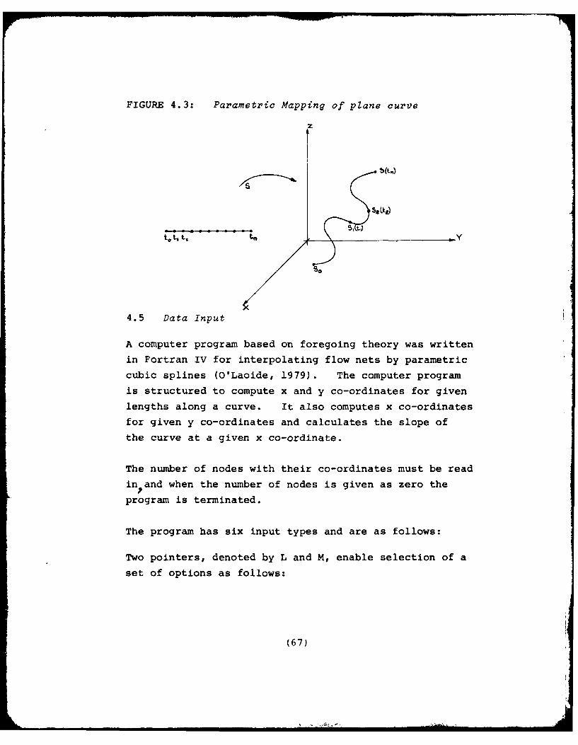
FIGURE 4.3: Parametric Mapping of plane curve

Z

to t,, Y

4.5 Data Input

A computer program based on foregoing theory was written

in Fortran IV for interpolating flow nets by parametric

cubic splines (O'Laoide, 1979). The computer program

is structured to compute x and y co-ordinates for given

lengths along a curve. It also computes x co-ordinates

for given y co-ordinates and calculates the slope of

the curve at a given x co-ordinate.

The number of nodes with their co-ordinates must be read

in and when the number of nodes is given as zero the

program is terminated.

The program has six input types and are as follows:

Two pointers, denoted by L and M, enable selection of a

set of options as follows:

(67)

L=l a length is read in and the corresponding x and

y co-ordinates are calculated

L=2 a length of increment is read in with an upper and

lower bound. The x and y co-ordinates for each

incremental length are calculated

L=3 an x co-ordinate is read in and its corresponding

y co-ordinate is calculated

L=4 an x co-ordinate increment is read in with an upper

and lower bound. The y co-ordinates for each

incremental x co-ordinate are calculated

L=5 an x co-ordinate is read in and the slope of the

curve at that co-ordinate is calculated

L=6 an x co-ordinate increment is read in with an upper

and lower bound, and the corresponding slopes

within the range are calculated.

When M = 0, for L = 1,2,3 and 4 the slopes corresponding

to the x co-ordinates will also be calculated. When M = 2

a cumulative chord length is read in and the corresponding

x and y coordinates are calculated.

4.6 Applications of Cubic Spline in Harmonic Analysis

Interpolation of Contour Intervals

Normally a spline is viewed as an ordinary function which

gives the value of the dependent variable for a pre-

scribed value of the independent variable (in a closed

interval). In what follows it is demonstrated that a

(68)

reverse process can be implemented whereby the dependent

variable can take on prescribed values and the original

independent variable can be treated as a dependent

variable. This transition provides a means of plotting

contours for monotonic functions and in particular

solutions of Lapace's equation with coordinates (x,y,

0) say, where 0 is the potential.

To map the contours we require ordinates at stations

along a grid line where the ordinates differ by a preset

value i.e. the contour interval. A cross-section on

any grid line will normally have contour ordinates at

irregularly spaced distances from the origin of the

cross section. Each contour ordinate t is locatedcat a root of the equation

Si( ) -t = 0 4.151

wnere Si ) is the spline function representing f14)

through the knots in the interval Ix, x1 + 11 or in

interval lyi, Yi + l( "

The roots of the Equation 4.15 can be determined with

any degree of accuracy by repeated application of the

Newton-Raphson formula, provided that there is no local

extremum of the function in the neighbourhood of a root.

This condition is satisfied by all harmonic functions

if sources and sinks are isolated in the physical

problem.

Reverting to the notation of the parametric cubic spline

Equation 4.2 and 4.15 are written in the form:

(69)

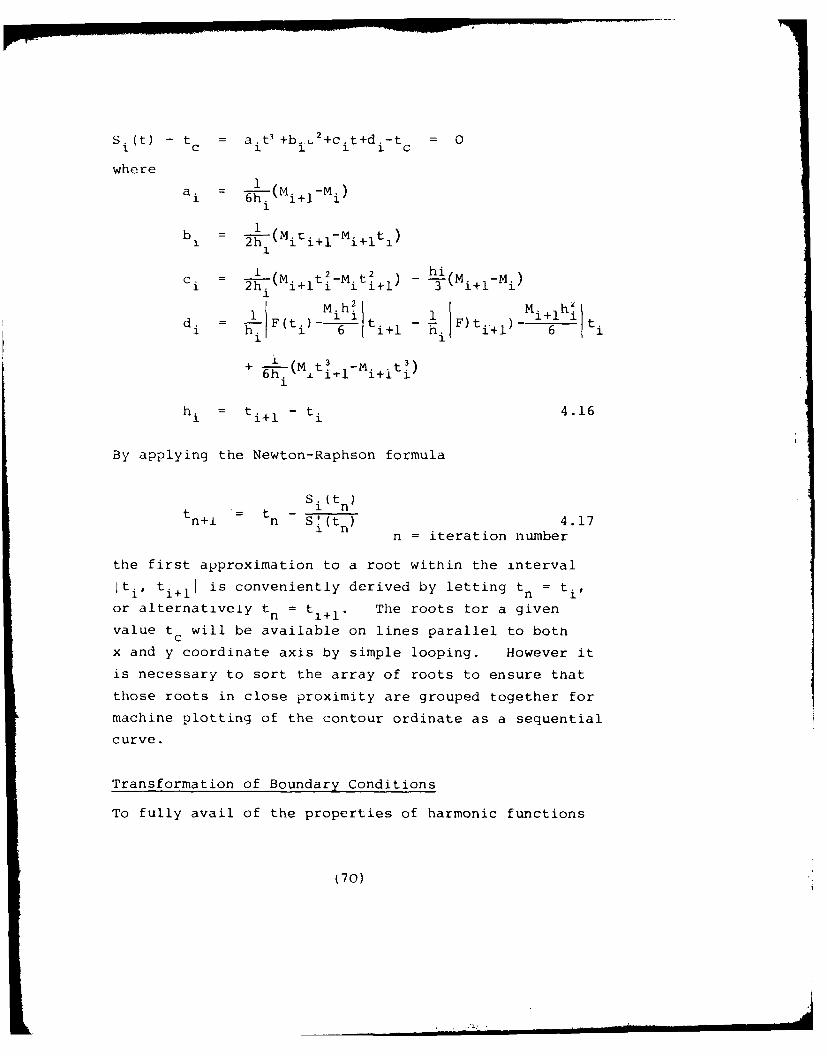
S (t) - t = a.t +b. 2+c.t+d.-t = O1. c 1 2. 1 1 C

where1ai - 6h. (i+l-i1

I 2h i i+l i+l

Ci I 2hii (Mi+t 2 -Mit2+ 1 ) -h(Mi-Mi)2hh i F) tf3+l)

1 M-h~jt 1 Mihzdi -1 F(ti)_p til F)t ih i-6 ~il h. i'+l 6 1

+ (M t? M t3)1 1

6h. ± i-tl- i+1

hi = ti+1 - ti 4.16

By applying the Newton-Raphson formula

S i (t n )n+ - n S'(t ) 4.17

n = iteration number

the first approximation to a root within the interval

Iti, ti+lI is conveniently derived by letting tn = tit

or alternativeiy tn = t The roots for a given

value tc will be available on lines parallel to both

x and y coordinate axis by simple looping. However it

is necessary to sort the array of roots to ensure that

those roots in close proximity are grouped together for

machine plotting of the contour ordinate as a sequential

curve.

Transformation of Boundary Conditions

To fully avail of the properties of harmonic functions

(70)

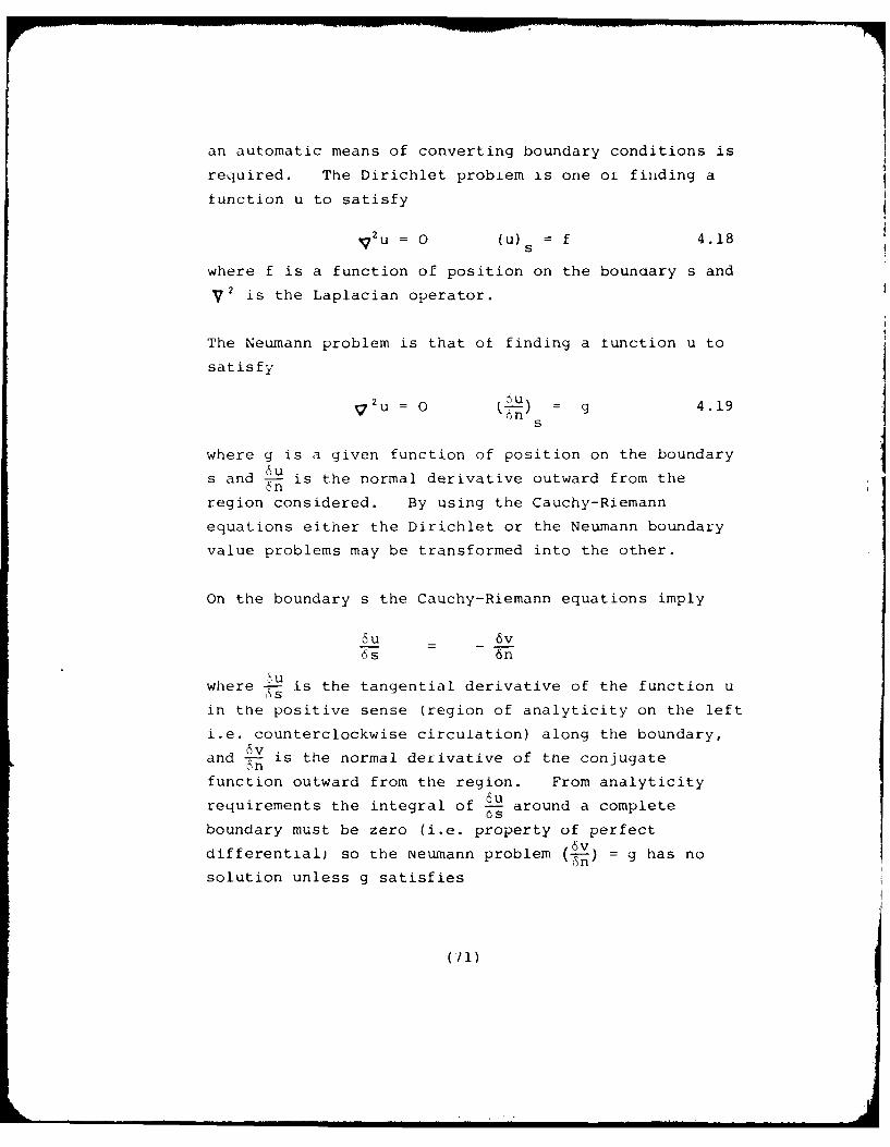
an automatic means of converting boundary conditions is

required. The Dirichlet problem is one or finding a

tunction u to satisfy

V2u = (u) s =f 4.18

where f is a function of position on the boundary s and

V 2 is the Laplacian operator.

The Neumann problem is that ot finding a tunction u to

satisfy

2 u = = g 4.19

ns

where g is a given function of position on the boundary

sand - is the normal derivative outward from the

region considered. By using the Cauchy-Riemann

equations either the Dirichlet or the Neumann boundary

value problems may be transformed into the other.

On the boundary s the Cauchy-Riemann equations imply

6u 6v6s 6n

where u is the tangential derivative of the function uSs

in the positive sense (region of analyticity on the left

i.e. counterclockwise circulation) along the boundary,

and Ax is the normal derivative of the conjugate

function outward from the region. From analyticityc u

requirements the integral of - around a complete

boundary must be zero (i.e. property of perfect6vdifferential) so the Neumann problem (-L-j ) = g has no

solution unless g satisfies

(11)

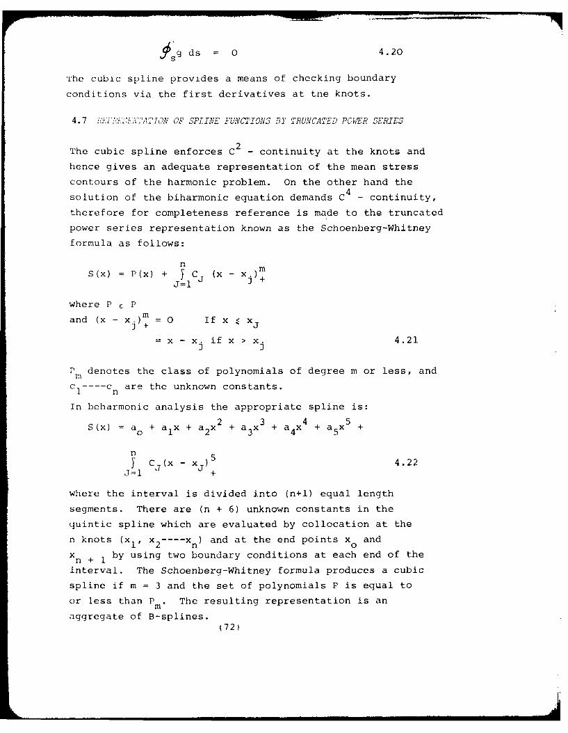
ds 0 4.20

ihe cubic spline provides a means of checking boundary

conditions via the first derivatives at tne knots.

4.7 iiAJ'L.V2ATION OF SPLINE FUNCTIONS BY TRUNCATED POWER SERIES

The cubic spline enforces C2 - continuity at the knots and

hence gives an adequate representation of the mean stress

contours of the harmonic problem. On the other hand the4

solution of the biharmonic equation demands C - continuity,therefore for completeness reference is made to the truncated

power series representation known as the Schoenberg-Whitney

formula as follows:

nS(x) = P(x) + Y Cj (x - x.)m

J=l +

where P E P

and (x xj)m+ = 0 If x

= x - x. if x > x. 4.213 3

Pm denotes the class of polynomials of degree m or less, andnnn -- are the unknown constants.

In beharmonic analysis the appropriate spline is:2 3 4 5

S(x) =a alx + a2x + a3x + a4x + a5x +

n $Y Cji(x - xj) 4.22

J=l +

where the interval is divided into (n+l) equal length

segments. There are (n + 6) unknown constants in the

quintic spline which are evaluated by collocation at the

n knots (xI , x2 ---- xn ) and at the end points x and

x n + 1 by using two boundary conditions at each end of the

interval. The Schoenberg-Whitney formula produces a cubic

spline if m = 3 and the set of polynomials P is equal to

or less than Pm . The resulting representation is an

aggregate of B-splines.(72)

CHAPTER 5

HARMONIC ANALYSIS OF STRESS FIELDS

I.

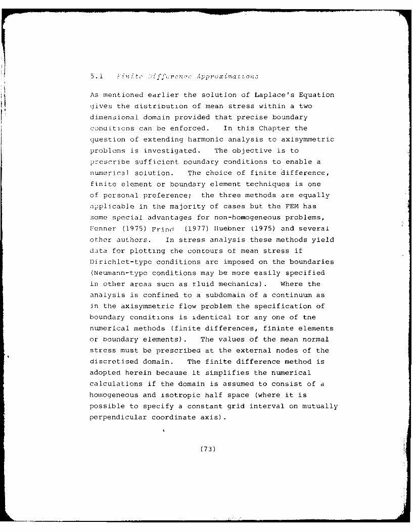
51 Fnzt frnc Approximnations-

As mentioned earlier the solution of Laplace's Equation

gives the distribution of mean stress within a two

dimensional domain provided that precise boundary

conaitions can be enforced. In this Chapter the

question of extending harmonic analysis to axisymmetric

problems is investigated. The objective is to

prescribe sufficient boundary conditions to enable a

numerical solution. The choice of finite difference,

finite element or boundary element techniques is one

of personal preference; the three methods are equally

applicable in the majority of cases but the FEM has

some special advantages for non-homogeneous problems,

Fenner (1975) Frin (1977) Huebner (1975) and several

other authors. In stress analysis these methods yield

data for plotting the contours ot mean stress it

Dirichlet-type conditions are imposed on the boundaries

(Neumann-type conditions may be more easily specified

in other areas sucn as tluid mechanics). Where the

analysis is confined to a subdomain of a continuum as

in the axisymmetric flow problem the specification of

boundary conditions is identical tor any one of tne

numerical methods (finite differences, fininte elements

or boundary elements). The values of the mean normal

stress must be prescribed at the external nodes of the

discretised domain. The finite difference method is

adopted herein because it simplifies the numerical

calculations if the domain is assumed to consist of a

homogeneous and isotropic half space (where it is

possible to specify a constant grid interval on mutually

perpendicular coordinate axis).

(73)

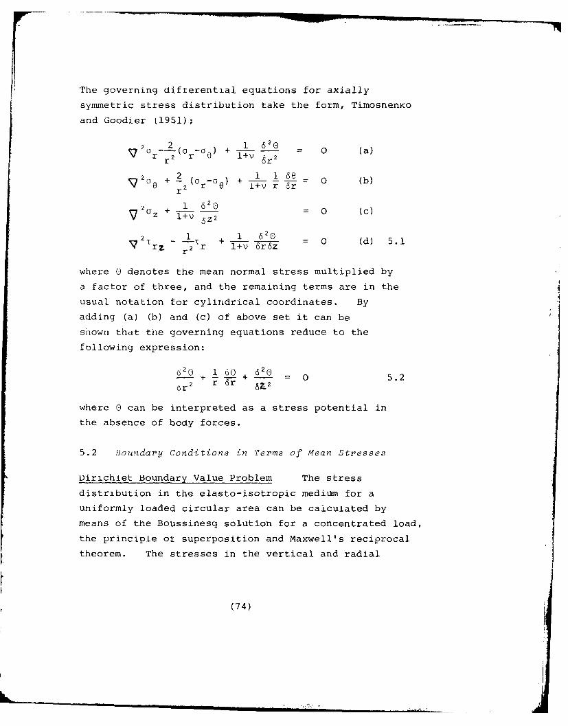
The governing cifterential equations for axially

symmetric stress distribution take the form, TimosnenKo

and Goodier (1951);

2O (r3 ) + 1 620 = 0 (a)

r r 2 i+v 6r2

V200 2 (0 + 1 16 = 0 (b)0 r2 r i+v r 6r

21 62 0 (c)IV2 z +V 6+Z2

2 1 -T + __L 620 0 (d) 5.1r z r2 r l+v 6r6z

where 0 denotes the mean normal stress multiplied by

a factor of three, and the remaining terms are in the

usual notation for cylindrical coordinates. By

adding (a) (b) and (c) of above set it can be

shown thdt the governing equations reduce to the

following expression:

0 2 1 60 620 0 5.2

or2 r 6r 672

where 0 can be interpreted as a stress potential in

the absence of body forces.

5.2 Boundary Conditions in Terms of Mean Stresses

Dirichiet Boundary Value Problem The stress

distribution in the elasto-isotropic medium for a

uniformly loaded circular area can be calculated by

means of the Boussinesq solution for a concentrated load,

the principle ot superposition and Maxwell's reciprocal

theorem. The stresses in the vertical and radial

(74)

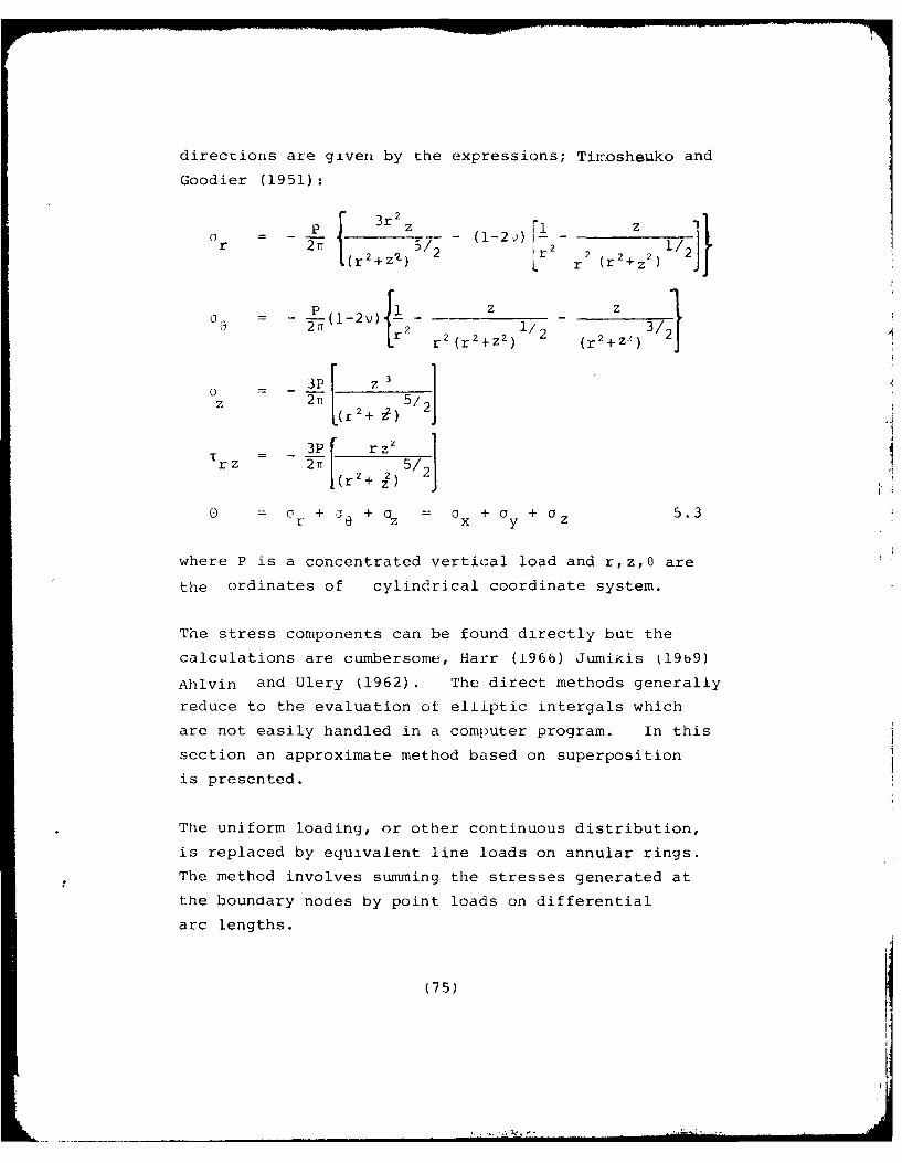
directions are given by the expressions; Tii.osheuko and

Goodier (1951):

P 3r2z - 2 2]}Or -2-- 5/ 1:2 1_ 1z

(r2+ Z.) /Lr r 2 r 2 Z2

z z0 -L.(l-2v){i - -312r2+Z2)/2 (r2+Z) 2

3= 3P r 3 ]z - 2--_ 5/2

(r2+ 2

+ - ++ 2?

r z x y z

where P is a concentrated vertical load and r,z,e are

the ordinates of cylindrical coordinate system.

The stress components can be found directly but the

calculations are cumbersome, Harr (196b) JumiKis k19b9)

Ahlvin and Ulery (1962). The direct methods generally

reduce to the evaluation ot elliptic intergals which

are not easily handled in a computer program. In this

section an approximate method based on superposition

is presented.

The uniform loading, or other continuous distribution,

is replaced by equivalent line loads on annular rings.

The method involves summing the stresses generated at

the boundary nodes by point loads on differential

arc lengths.

(75)

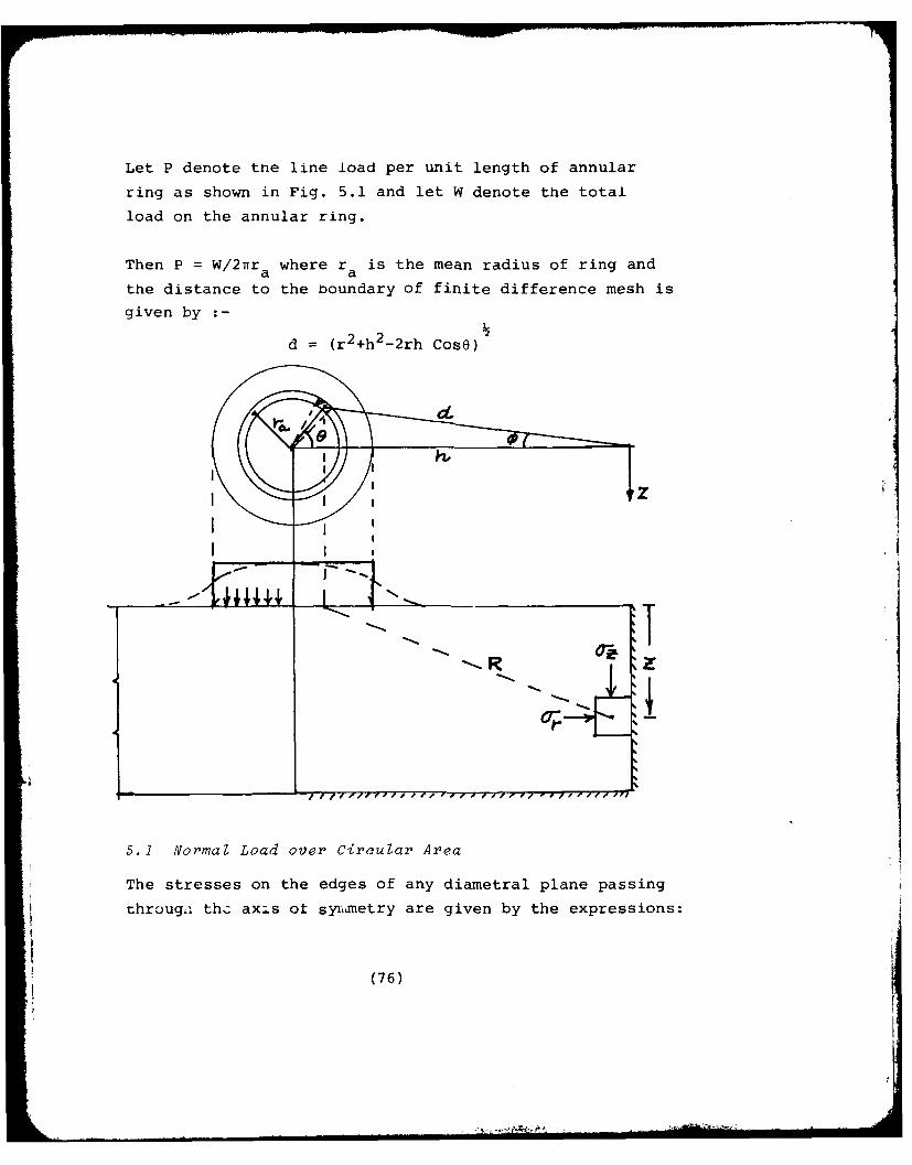
Let P denote the line load per unit length of annular

ring as shown in Fig. 5.1 and let W denote the total

load on the annular ring.

Then P = W/2mra where ra is the mean radius of ring and

the distance to the noundary of finite difference mesh is

given by

d - (r2+h 2-2rh CosO)

%T_*

I lle

5.1 Normal Load over Circular Area

The stresses on the edges of any diametral plane passing

througi th axis ot syr,,metry are given by the expressions:

(76)

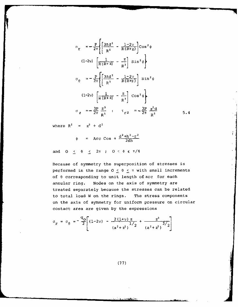
0 P f 3zd 2 1-2v C1 20r 2tYr 1 R5 R(-R+z)

(1-2v) _ 1 Sin4

P[3zd 2 1-2v Sin 2

2 Tr IR 5 R (R+z)

(1-2v) [Z3COS2i}3P z' 3P Z2 d

where R 2 z 2+d2

= Ar~os+ 2dh

and 0 < 0 < 2ff 0 <~ (D 4/

Because of symmetry the superposition of stresses is

performed in the range 0 < 6 < ff with small increments

of 0 corresponding to unit length of arc for each

annular ring. Nodes on the axis of symmetry are

treated separately because the stresses can be related

to total load W on the rings. The stress components

on the axis of symmetry for uniform pressure on circular

contact area are given by the expressions

a G L[(12v) V +(~~ 1/ -

(77)

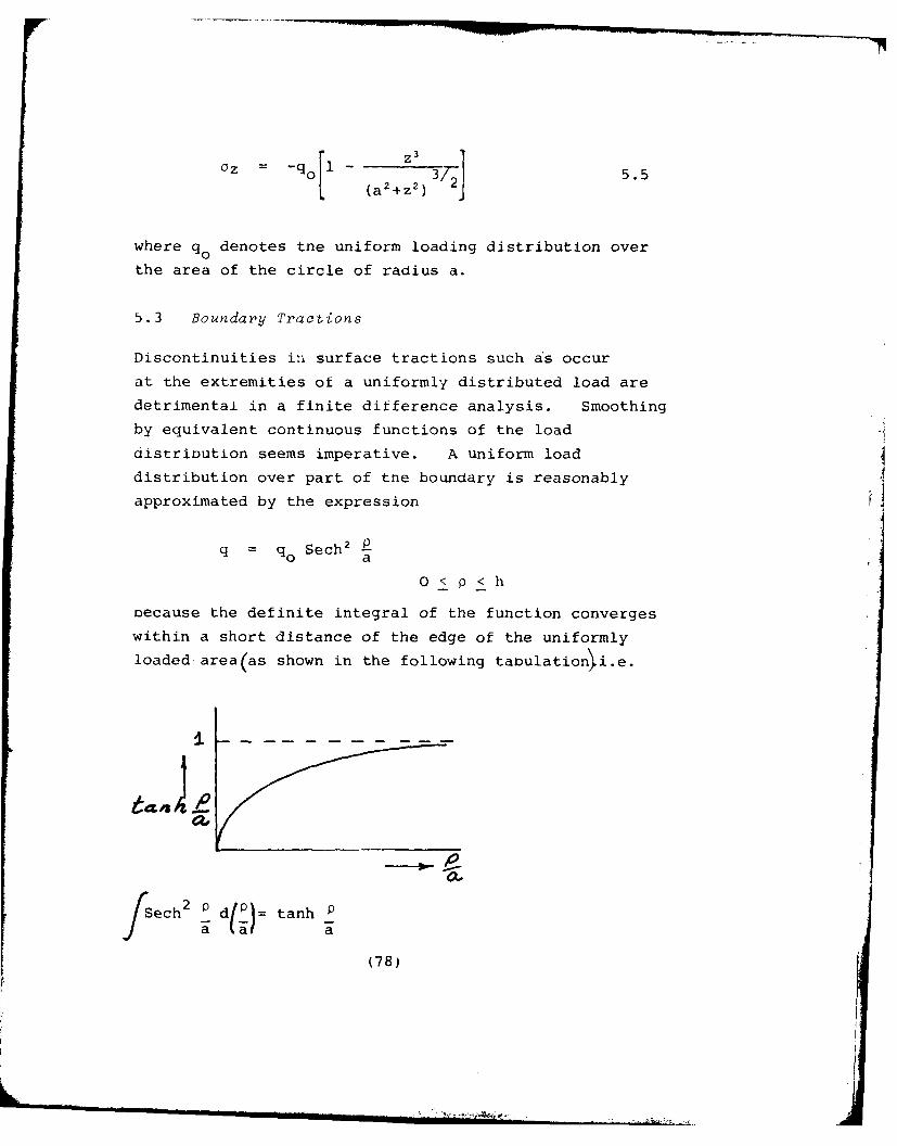
z= Fo-qo[l Za 3/ 5.5

(a2+z 12 )

where q0 denotes tne uniform loading distribution over

the area of the circle of radius a.

5.3 Boundary Tractions

Discontinuities in surface tractions such as occur

at the extremities of a uniformly distributed load are

detrimental in a finite difference analysis. Smoothing

by equivalent continuous functions of the load

distribution seems imperative. A uniform load

distribution over part of the boundary is reasonably

approximated by the expression

q = q Sech2P

O~zp<h

because the definite integral of the function converges

within a short distance of the edge of the uniformly

loaded area(as shown in the following tanulationi.e.

f/Sech 2 d tanh P

(78)

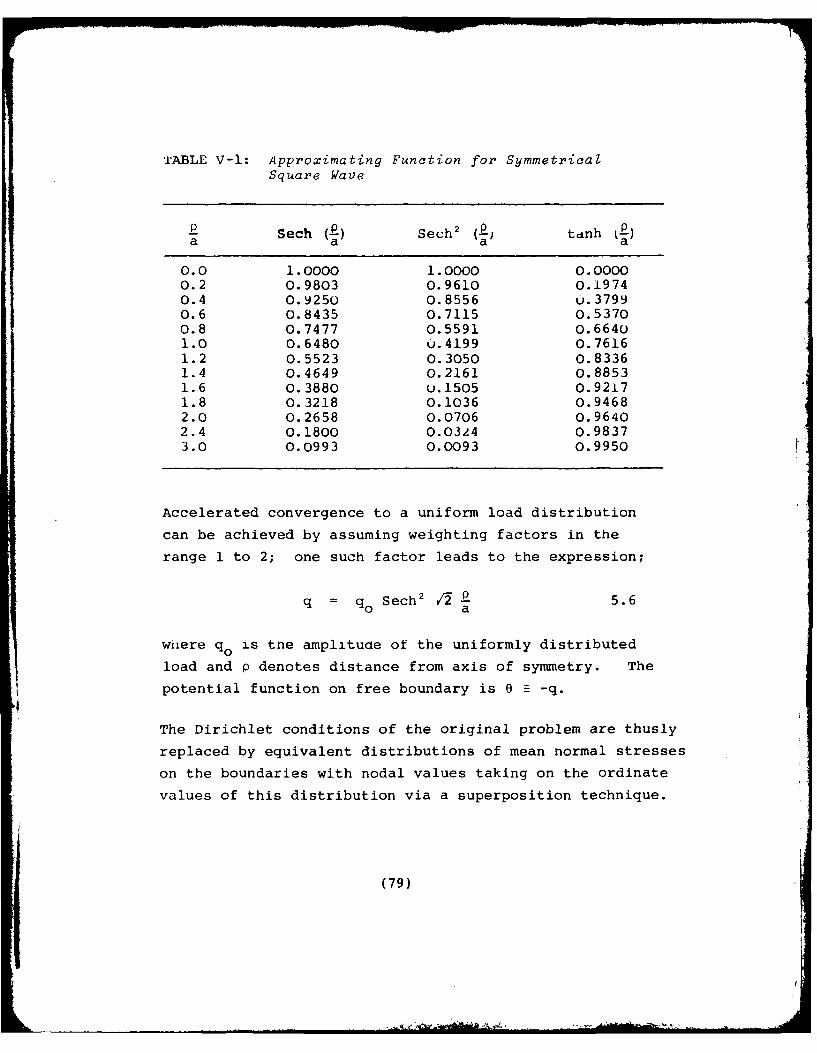
TABLE V-1: Approximating Function for SymmetricalSquare Wave

a Sech (P) Sech 2 (j tanh tP)a a a a

0.0 1.0000 1.0000 0.00000.2 0.9803 0.9610 0.19740.4 0.9250 0.8556 u.37990.6 0.8435 0.7115 0.53700.8 0.7477 0.5591 0.66401.0 0.6480 u.4199 0.76161.2 0.5523 0.3050 0.83361.4 0.4649 0.2161 0.88531.6 0.3880 u.1505 0.92171.8 0.3218 0.1036 0.94682.0 0.2658 0.0706 0.96402.4 0.1800 0.0324 0.98373.0 0.0993 0.0093 0.9950

Accelerated convergence to a uniform load distribution

can be achieved by assuming weighting factors in the

range 1 to 2; one such factor leads to the expression;

q = q Sech 2 V/2 5.60 a

where q is tne amplitude of the uniformly distributed

load and p denotes distance from axis of symmetry. The

potential function on free boundary is 0 = -q.

The Dirichlet conditions of the original problem are thusly

replaced by equivalent distributions of mean normal stresses

on the boundaries with nodal values taking on the ordinate

values of this distribution via a superposition technique.

(79)

. &O-Uk-

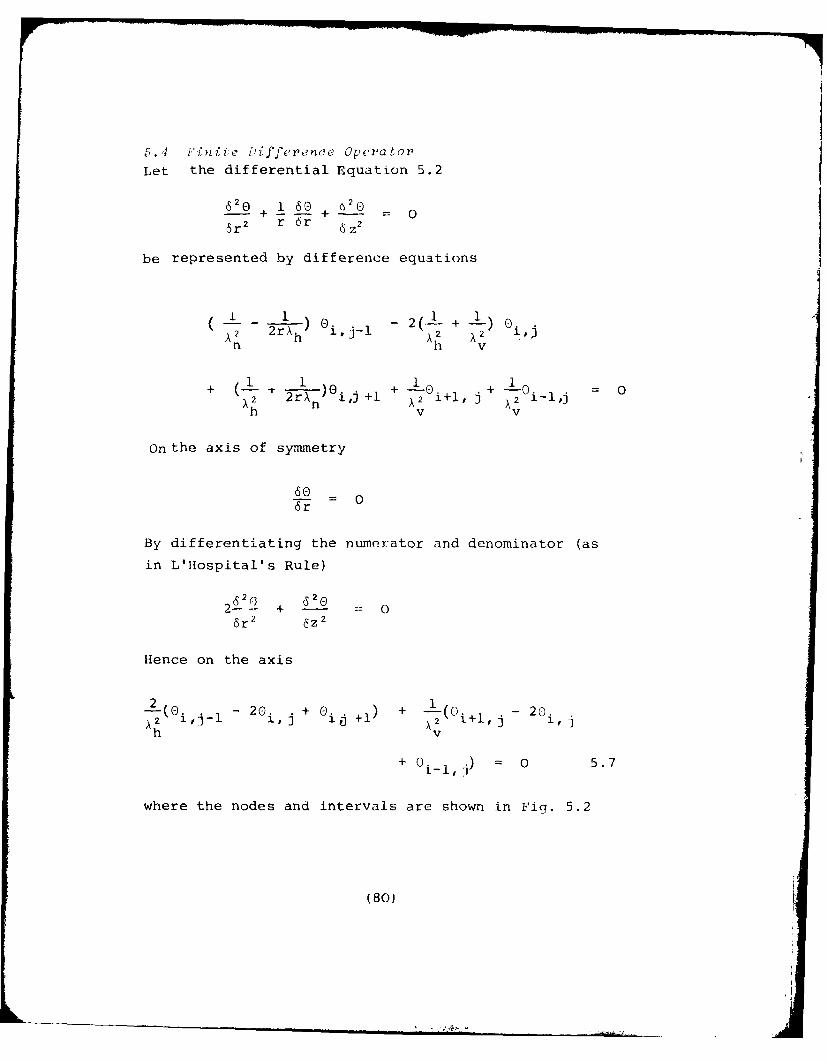
54 1' nite fPiffer,3nce Opcrator

Let the differential Equation 5.2

620 1 60 =® 0

6r2 r 6r 6 Z2

be represented by difference equations

I - -1 e..E -2(-1 + 1) 02 2rA h h ij-i x2 x2 ''jAn h v

+( 1 1 ) -- + = 02 2r n eIj +1

2 i+l, + 2 i-l,jh v v

On the axis of symmetry

606r

By differentiating the numerator and denominator (as

in L'Hospital's Rule)

2-2 + -0 o6r2 6z 2

Hence on the axis

-(.i2. . -0- 20.iA2 (0i l 20, j + ij +j) + 1(0i+l, j 2, jh v

+ 0 j) 0 0 5.7

where the nodes and intervals are shown in Fig. 5.2

(80)

I.

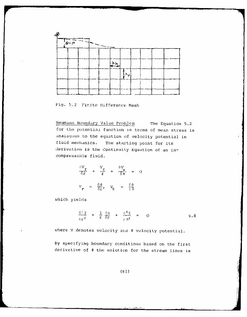
Fig. 5.2 Finite DifferencE Mesh

Neumain Boundary Value Problem The Equation 5.2

for the potential function in terms of mean stress is

analaqous to the equation of velocity potential in

fluid mechanics. The starting point for its

derivation is the Continuity Equation of an in-

compressible fluid.

v v 6Vr + -- + .7. - ()6r r 6z

r Sr' Vz Z

which yields

+ + 0 5 82 r 6r z2

where V denotes velocity and $ velocity potential.

By specifying boundary conditions based on the first

derivative of P the solution for the stream lines is

(ei)

obtaLned. The Neumann problem is posed by taking as the

Continuity Equation the e:pression

6V 15Vr z -O

6z 6r

r r 6z' z C

which yields

-0 5.96r 2 r 6r 6z2

where the boundary conditions are those discussed in Chapter 4.

The solution of the Neumain problem can be extracted to within

an arbitrary constant throujhout the domain. There are

sufficient data for contouring lines of constant 9, and in fact

the same solution routine can be used for finding # and

simply by inserting a linking subroutine to generate the

values at the nodes of the boundary. An interesting variant

of this approach has been reported for the problem of seepage

through an earth dam, Shaug and Bruch (1976). However, for the

stress distribution problem the Neumann conditions pertain to

strain energy density which are difficult to prescribe. Hence

an alternative method is required for finding orthogonal

trajectories to the mean stress contours.

The problem of orthogonal slip-line fields is extensively

covered in applications of plasticity theory, hence as a

preliminary to the present author's approach to potential field

problems a brief outline of mechods employed in plastic analysis

is included in the next section.

(82)

5.5 Slip-Line Fields in Plasticity Theory

Method of Characteristics

The theory of the ideal plastic solid yields differential

equations for solution of the geometrical constraints on the

slip lines. For the case of plane strain the governing

differential equation is derived on the following assumptions:-

1. the shear stress has a yield value k which is induced

at every point on a slip line,

2. the equilibrium equations are identical to those of

elasticity theory,

3. the direct stress normal to the slip line is the mean

stress devoted by

4. the geometrical constraints on the slip lines can be

referred to Cartesian coordinates with the angle subtended

by normal to the plane of maximum shear and the x-axis the

identifying parameter (denoted by a) as depicted in Fig. 5.3.

Consider a homogeneous weightless material in a state of

limiting equilibrium. The equilibrium equations are given by

the expressions, Unksov (1961):-

6a 6X + xy= 0

6x 6y

6 6axy+ _ = 0 5.106x 6y

and the stress state in terms of o and k is as follows:-

o = a + k Sin 2ax

k =-kSin 2ay

Txy -k Cos 2a 5.11

(83)

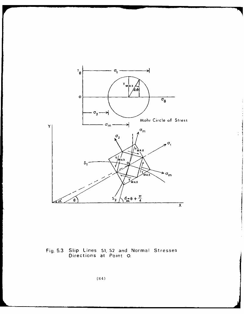
T C '

0 2

Mohr Circle of Stress

y am

0F2

510

MAx

Fig. 5.3 Slip Lines S1, S2 and Normal StressesDirections at Point 0.

(84)

By substituting the expressions 5.11 into 5.10 the

equilibrium equations in terms of the mean stress become:606a

T- + 2k(Cos 2a± + Sin 2a -) = 06x 6Xy

6- 2k(Cos 2a6 - Sin 2a -) = 0 5.12Ti 6y 6x

On eliminating o, by differentiating the first of 5.11 with

respect to x and the second to y the single differential

equation is obtained by subtraction viz.

---- + 2 Cot 2a 6a+ -- 4 6-a +6X 2 6x6y y2 6x 6y

2 Cot ra)2 - (1a)2 0 5.136y 6X

By the theory of differential equation the so-called

characteristic equation for 5.12 is given by

- dy2 - 2 Cot 2a dx dy + dx 2 = 0 5.14

The roots of equation 5.13 are both real i.e. the equation

5.12 is hyperbolic, and lead to the solution for the

characteristic directions as follows:

- = - Cot 2a + (Cot2 2a + 1)0dx 1

+Cos2a 1 = tansSin 2 + Sin 2a

Cot 2a (Cot 2 2a + 1)0 Cotad 2 5.15

It follows that the tangents to the slip lines at any point

form angles with the x-axis which are given by the equalities

(85)

NUMERICAL METHDS FOR CREEP ANALYSIS IN GEOTECHNICAL PROBLEMS. (U)DEC A1 T E GLYNN DAERO-76-6-063

UNCLASSIFIED NL

DTl l l l l lf f f f f f

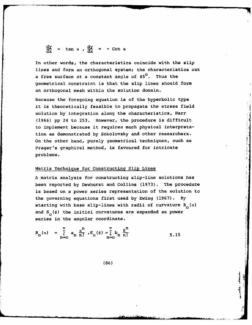
= tan d = -Cotadx 'dx

In other words, the characteristics coincide with the slip

lines and form an orthogonal system; the characteristics cut

a free surface at a constant angle of 450. Thus the

geometrical constraint is that the slip lines should form

an orthogonal mesh within the solution domain.

Because the foregoing equation is of the hyperbolic type

it is theoretically feasible to propagate the stress field

solution by integration along the characteristics, Harr

(1966) pp 24 to 253. However, the procedure is difficult

to implement because it requires much physical interpreta-

tion as demonstrated by Sokolovsky and other researchers.

On the other hand, purely geometrical techniques, such as

Prager's graphical method, is favoured for intricate

problems.

Matrix Technique for Constructing Slip Lines

A matrix analysis for constructing slip-line solutions has

been reported by Dewhurst and Collins (1973). The procedure

is based on a power series representation of the solution to

the governing equations first used by Ewing (1967). By

starting with base slip-lines with radii of curvature R o(c)

and So(M) the initial curvatures are expanded as power

series in the angular coordinate.

O n Wo nRo(cz) = an .'So().'510 IaS( =1 bn '~51n=o n=o

(86)

V

I

----- -----------------

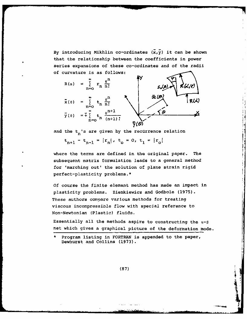
By introducing Mikhlin co-ordinates (x,y) it can be shown

that the relationship between the coefficients in power

series expansions of these co-ordinates and of the radii

of curvature is as follows:en Y V

R(a) = rn. ISn=o

) t -tn=o n n

coln+1y(e) =T I t n

n=o n (n+l)! V*1

and the t 's are given by the recdrrence relation

t - tn_ Irnl to = 0, tI = Iroln+l n-1 n'

where the terms are defined in the original paper. The

subsequent matrix formulation leads to a general method

for 'marching out' the solution of plane strain rigid

perfect-plasticity problems.*

Of course the finite element method has made an impact in

plasticity problems. Zienkiewicz and Godbole (1975).

These authors comnare various methods for treating

viscous incompressible flow with special reference to

Non-Newtonian (Plastic) fluids.

Essentially all the methods aspire to constructing the a-8

net which gives a graphical picture of the deformation mode.

* Program listing in FORTRAN is appended to the paper,

Dewhurst and Collins (1973).

(87)

5.6 Orthogonal Trajectories to Countoure of Mean Stresaes:

A New Numerical Method.

In the course of this study it became evident that a

technique more versatile than that presented in Chapter 3

is needed. In particular if the special attributes of para-metric splines are to be exploited for plotting trajectories

of mean and shear stresses a solution format analogous to

the matrix method for plasticity is a desirable goal. Apartfrom applications of complex variable theory and trial and

error sketching of flow nets no techniques emerged from an

extensive literature search. The present author expended

considerable effort to simply find a framework for theproblem, because there are a number of possible formulations,

for instance, such as differential forms, optimization

theory or indeed eigenvalue solutions. It transpires thatoptimization theory affords the most tangible approach and

is the basis of the method proposed herein.

Inspection of the plots of orthogonal nets produced by the

harmonic analysis of Chapter 3 indicated that each set of

trajectories of the c-a net are the envelopes of a family

of circles as illustrated in Fig. 5.4. By assuming that

points of tangency of certain members of the infinite set

of circles bounded by the mean stress contours lie on the

required trajectory, the optimization problem for finding

the locus of the centres reduces to the statement:

'Given two non intersecting curves in a plane find the

family of circles that meets the constraint of tangency

to the given curves and in addition ensures that no one

member of the family intersects any other member.'

(88)

sj

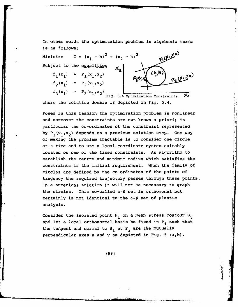
In other words the optimization problem in algebraic terms

is as follows:

Minimize C = (x -h) 2 + (x 2 -k)2

Subject to the equalitiesi xl

f2 (x1 ) = P2 (xlX 2 )

f 3 (x1 ) = P3 (xlx 2 )Fig. 5.4 Optimization Constraints

where the solution domain is depicted in Fig. 5.4.

Posed in this fashion the optimization problem is nonlinear

and moreover the constraints are not known a priori; in

particular the co-ordinates of the constraint represented

by P3 (XlX 2 ) depends on a previous solution step. One way

of making the problem tractable is to consider one circle

at a time and to use a local coordinate system suitably

located on one of the fixed constraints. An algorithm to

establish the centre and minimum radius which satisfies the

constraints is the initial requirement. When the family of

circles are defined by the co-ordinates of the points of

tangency the required trajectory passes through these points.

In a numerical solution it will not be necessary to graph

the circles. This so-called a-$ net is orthogonal but

certainly is not identical to the a-$ net of plastic

analysis.

Consider the isolated point Pi on a mean stress contour Siand let a local orthonormal basis be fixed in Pi such that

the tangent and normal to Si at Pi are the mutually

perpendicular axes u and v as depicted in Fig. 5 (a,b).

(89)

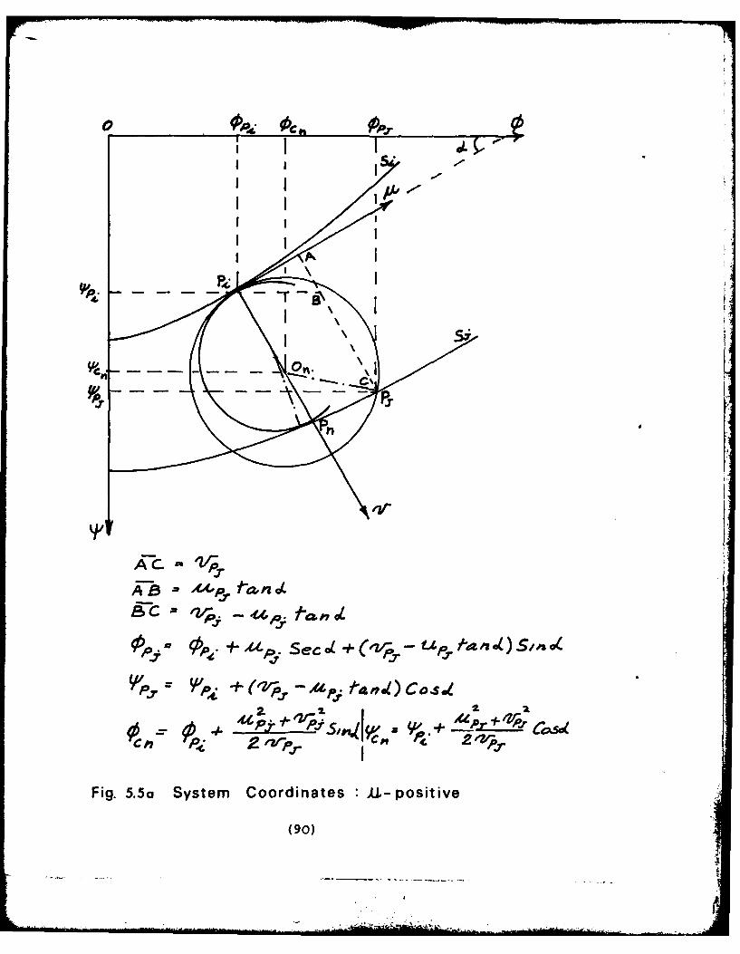
i I I ,,

I I 4

+ 1 e

• \

II

Fig. 5.5o System Coordinates •l-positive

(90)

......... .~ ~ ~ ~ ...... ------. _- . ,i ,s -i. ' ,

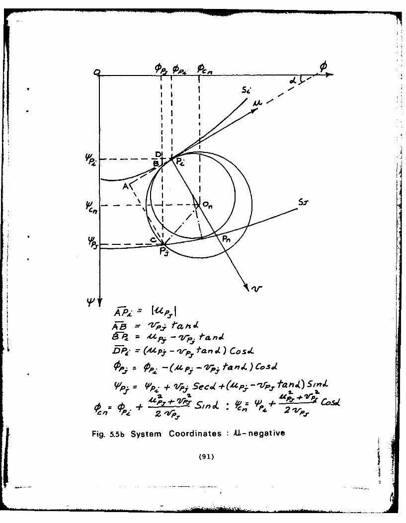
I MI 1000,Ii

II I / kI

I t

Ii I'I

2. I

Fi . -Systemj Cooprdiae iLL-negative

(91) i

I

OnI

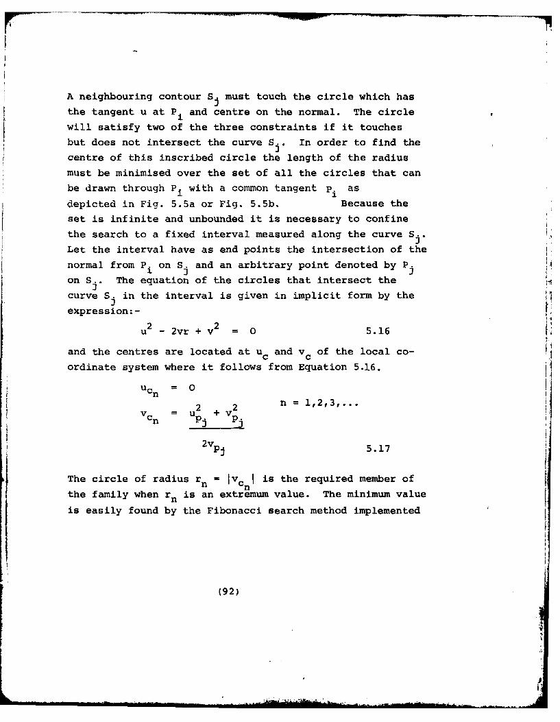
A neighbouring contour Si must touch the circle which hasthe tangent u at Pi and centre on the normal. The circlewill satisfy two of the three constraints if it touchesbut does not intersect the curve S. In order to find thecentre of this inscribed circle the length of the radiusmust be minimised over the set of all the circles that can

be drawn through Pi with a common tangent pi as

depicted in Fig. 5.5a or Fig. 5.5b. Because theset is infinite and unbounded it is necessary to confinethe search to a fixed interval measured along the curve S -.

Let the interval have as end points the intersection of thenormal from P. on S. and an arbitrary point denoted by P.

on S.. The equation of the circles that intersect thecurve S. in the interval is given in implicit form by theJexpression:-

2 v2u- 2vr + = 0 5.16

and the centres are located at uc and v c of the local co-ordinate system where it follows from Equation 5.16.

Uc = 0n

Vcn = U. + ..

n Pi

2vpj 5.17

The circle of radius rn = IvcnI is the required member of

the family when rn is an extremum value. The minimum value

is easily found by the Fibonacci search method implemented

(92)

by sampling along the curve S. in the prescribed interval.*J

The remaining constraint is satisfied by insisting that

two neighbouring circles bounded by Si and S. have their

centres separated by the sum of their respective radii

taken along the curve joining the centres. To implement

this constraint let the initial trial circles intersect

i.e. the radical axis lies on both circles. In subsequent

steps the intersection on the classical Venn-type diagram

is reduced to a null set which then satisfies the third

constraint.

Thus far the point Pi is arbitrarily positioned on the

curve S. In order to locate the first trajectory to Si

we need a symmetry axis where the circle that starts the

process can be defined without resort to the search

technique. The radius of the initial circle in each flow

tube is calculated from the intercept of S. and S. on the

axis of symmetry. It transpires that a good first approxi-

mation to the location of Pi is given by offsetting Pi a

distance of 2r along the curve S. where r representsa a

the radius of the predefined circle. The point P. is

located at a distance ra along S . For either parallel

or diverging curves (Si and S.) this choice ensures that

the first trial circle intersects the previous best fit

to the given constraints. The final position of Pi on

The search employs the Fibonacci sequence of integer

values given by:

n-

Alternatively a tabulation of sampling stations based

on this formula is available. Henley and Williams

(1972). (93)

(93)

i

I

the curve Si is found by iteration using as incremental

steps the distances A given by the Expression 5.18 and

repeated application of the Fibonacci search,

2rn+l 6 5.18A =

rn + rn+ 1

where 6 denotes the overlap of the two circles alonl

the curve through their centres cf. Fig. 5.6

rn and rn+l are the radii of the neighbouring circles.

If the curves Si and S. derive from a functional relation-)ship such as the Eqn. 5.3, it merely remains to relate

the local coordinate system to the global axes. For the

sake of generality the point Pj is taken to right of the

normal P in addition to the left of the point which is thendesired location of P. in this context as shown in Fig. 5.5.b

The coordinate systems provide the relationships:

= . - (up - v tana)cosa

P = P + vp. seca + (up - vp tana)sina

5.19

where tanc is the slope of the tangent at Pi, and (0 ,pp p

represent global coordinates of points on the mean stress

contours. By matrix inversion the values of upVp become

the dependent variables required for evaluating the radii

of the inscribed circles. Of course in a computer programit is not necessary to graph the circles; the global co-

ordinates of the points of tangency and the location of

centres is all that is required from the iteration process.

(94)

~Jit

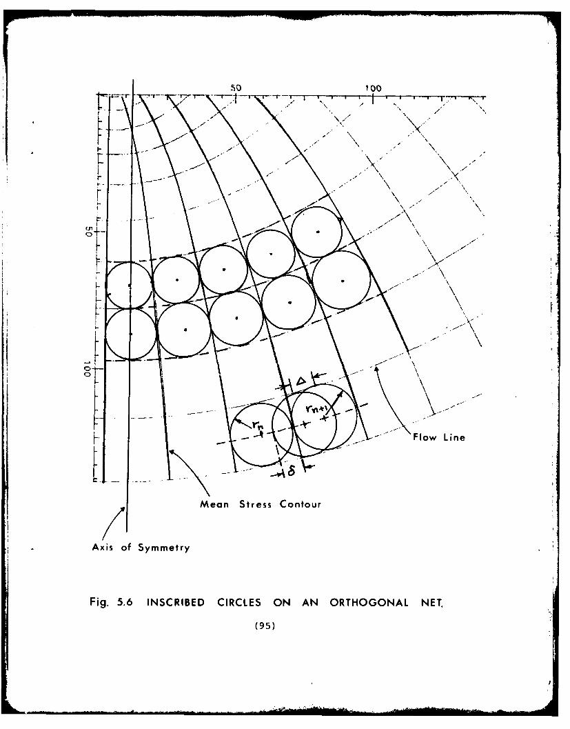
50 100

A~tr~~Fo LineT t1~

Mea Stres Conou

Axi of Sy mer

Fig- 5.6 INCIE CICE N A RHG N L NT

(95)A

The trajectories representing the flow lines pass through

the contact points of the inscribed circles, hence it is

necessary to generate a curve through the centres of the

circles, and subsequently to find the contact points by

offsetting chord lengths along the median curve equal to

the sum of the radii of all feasible circles within the

flow tube.

At first sight the procedure outlined above might seem

complicated; in fact it is a straightforward programming

exercise with only one exceptional difficulty. The

difficulty forecasted is that of finding the intersection

point of the normal which bounds the search level. The

difficulty is exacerbated by the use of parametric cubic

splines. The normal at the point Pi(i,Ti) is given by

(cf. Fig. 5.5):

- =0 ) cot

and the spline fit to Sj is of the form (Equation 4.16):

= alt 3 + b.t 2 + cjt + dj1J J

= eJt3 + f t2 + gJt + hj

Thus, the coordinates of the intersection must be deduced

by solving for the parameter t between those three

equations and subsequently finding the global coordinates

represented by t. Here the t-parameter is one of the

roots of a cubic equation viz.

(aj cots + ej)t 3 + (bj cots + fj)t 2 + (cj cots + gj)t +

k =0

where k= + e1cot- hj - djcotto

5.20(96)

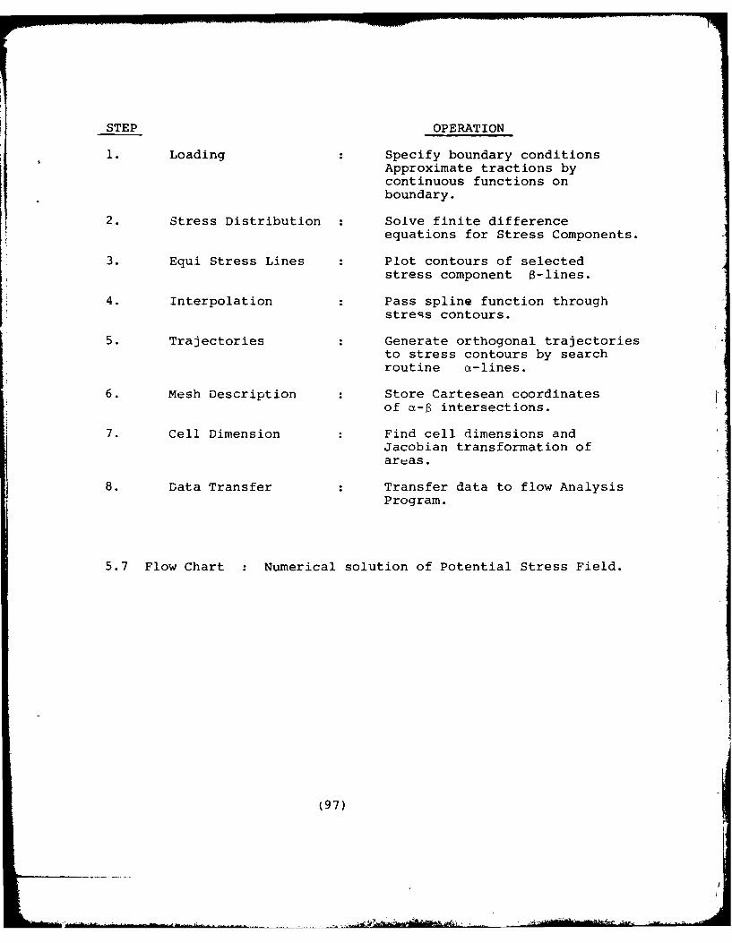
STEP OPERATION

1. Loading Specify boundary conditionsApproximate tractions bycontinuous functions onboundary.

2. Stress Distribution Solve finite differenceequations for Stress Components.

3. Equi Stress Lines Plot contours of selectedstress component s-lines.

4. Interpolation Pass spline function throughstreqs contours.

5. Trajectories Generate orthogonal trajectoriesto stress contours by searchroutine c-lines.

6. Mesh Description Store Cartesean coordinatesof a-6 intersections.

7. Cell Dimension Find cell dimensions andJacobian transformation ofare-as.

8. Data Transfer Transfer data to flow AnalysisProgram.

5.7 Flow Chart Numerical solution of Potential Stress Field.

(97)

Because of multiple roots of which only one is relevant, the

Eqn. 5.20 can prove a nuisance in numerical solutions. Indeed,

the main difficulty arises from the fact that the constants

a., bj etc. are specific to the knots on the spline and

hence it is necessary to specify the regime of parameter

t beforehand. One can only hope that this problem can be

resolved by neat programming! If this drawback is removed

it may even become practicable to find the coordinates of

the intersection of the trajectories which is regarded as

the final (but not essential) step in the proposed method.

The procedure is illustrated by the flowchart in Fig. 5.7.

(98)

CHAPTER 6

FINITE ELEMENT ANALYSES OF CREEP

AND

CONTINUUM MECHANICS

I.

Ii*1i

• *1

6.1 Introduction

In this Chapter a brief review of the application of

finite elements is presented as background to further

development of the method in this research project.

The review is mainly prepared from the formulation

given by Penny and Marriott (1971); this treatment

is elementary but has the appeal that it contains the

fundamentals which form the basis of subsequent

literature on the topic. The present author has

endeavoured to concentrate on those sections that are

not held in common by the various contributors (as

for instance the peripheral development of solution

routines for time stepping/instability caused by ill-

conditioned matrices and like problems). The

author's contribution centres around the manipulation

of reference frames and the handling of creep test

data in analyses.

6.2 Summary of Matrix Displacement Method

The initial loading problem is solved first; initial

strains due to plasticity, creep, thermal variations

are denoted by a vector {c } and the matrix algebra

is in the usual notation. Superscript 'e' refers

to element quantities. Subscript 'el' refers to

elastic properties and subscript c to creep.

Primed quantities refer to local element coordinates.

The procedure is as follows:

(99)

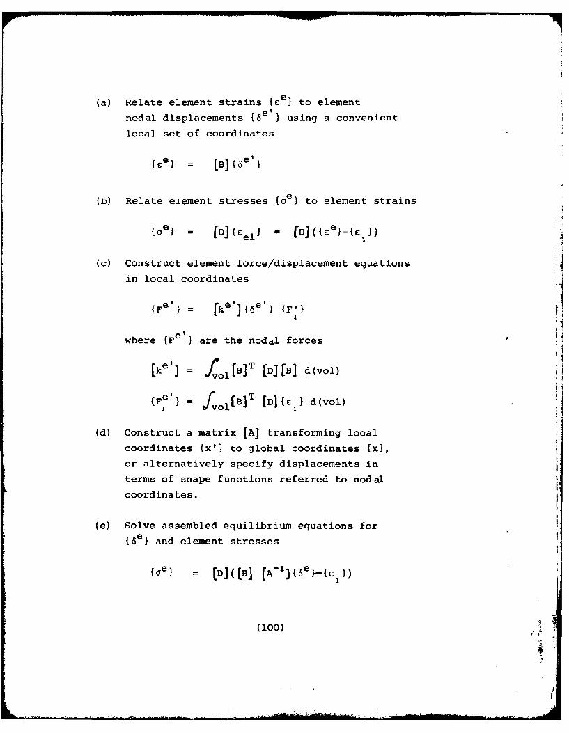
(a) Relate element strains { e} to element

nodal displacements [6e'} using a convenient

local set of coordinates

{e} = [B] {6e}

(b) Relate element stresses {e} to element strains

e = fD]el = D1({je}-{c I)

(c) Construct element force/displacement equations

in local coordinates

1 H{Fe ' [k s 6 {F'}

where {Fe '} are the nodal forces

[ke ' ] /vol[B]T [D][B] d(vol)

{Fe} v BT ID] {E d(vol)1 = ~ol ~ 1

(d) Construct a matrix [A] transforming local

coordinates {x'} to global coordinates {x},

or alternatively specify displacements in

terms of shape functions referred to nodal

coordinates.

(e) Solve assembled equilibrium equations for{e} and element stresses

{0 e} = [D]([B] [A-']{6e}-{E })

(100)(zoo) ?

J;

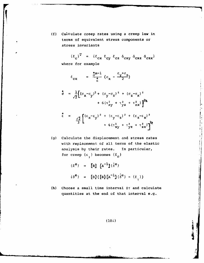
(f) Calculate creep rates using a creep law in

terms of equivalent stress components or

stress invariants

C} = cx cy cz acxy cxz czx}

where for example

0 +o*m-1 a +acx - * (Ox 2C

l[(oxGy)2 + (ay-aa) 2 + (Cz_(x) 2

+ 6 (T2 +1T2+T2xy yz zx )

* = [ 2 I 2 . f(Ex_ey) + (yEz) + (Z 2

3 + 6(T2 2 +12X yz zx)3

(g) Calculate the displacement and stress rates

with replacement of all terms of the elastic

analysis by their rates. In particular,

for creep { II becomes {c I1C

{el= [B] (A-]{6 e }

{ [D(B[A - )

(h) Choose a small time interval AT and calculate

quantities at the end of that interval e.g.

(101)

I:

( ioi )

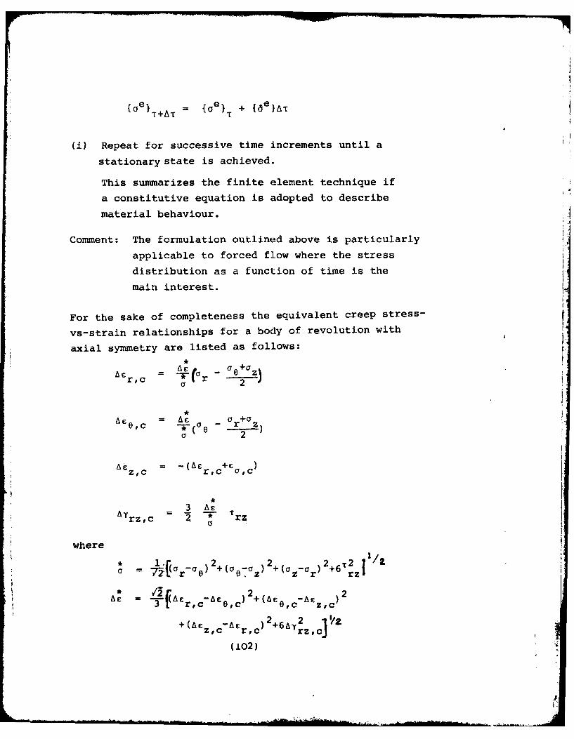
{eT+A = {oe} + {WeA

(i) Repeat for successive time increments until a

stationary state is achieved.

This summarizes the finite element technique if

a constitutive equation is adopted to describe

material behaviour.

Comment: The formulation outlined above is particularly

applicable to forced flow where the stress

distribution as a function of time is the

main interest.

For the sake of completeness the equivalent creep stress

vs-strain relationships for a body of revolution with

axial symmetry are listed as follows:*

a +ar = (or - 2o~zSr,c 2

Ac = Ac -- 0,c -r z

o2

~zc = -(Ac-9+E66Zz ,c -( cr ,c +C O c

3 Acrz,c rz

where

1 1- 2 2 2 T2 7/

7 a 1 0r-ae) +(a0oZ) +(o-o) +6 rz'

3 = Ar,c-e,c) 2+ c-zc

+(Ac -Ac 2 +6Ay /2z,c r,c rz,cj

(102)

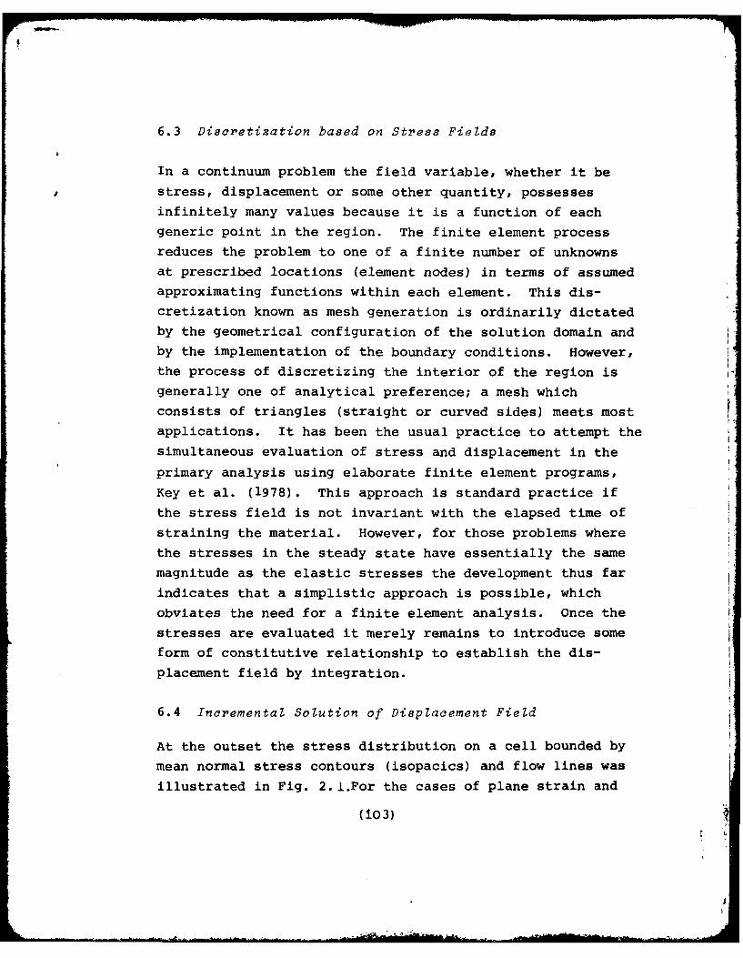
6.3 Discretization based on Stress Fields

In a continuum problem the field variable, whether it be

stress, displacement or some other quantity, possesses

infinitely many values because it is a function of each

generic point in the region. The finite element process

reduces the problem to one of a finite number of unknownsat prescribed locations (element nodes) in terms of assumed

approximating functions within each element. This dis-

cretization known as mesh generation is ordinarily dictated

by the geometrical configuration of the solution domain and

by the implementation of the boundary conditions. However,

the process of discretizing the interior of the region is

generally one of analytical preference; a mesh which

consists of triangles (straight or curved sides) meets most

applications. It has been the usual practice to attempt the

simultaneous evaluation of stress and displacement in the

primary analysis using elaborate finite element programs,

Key et al. (1978). This approach is standard practice if

the stress field is not invariant with the elapsed time of

straining the material. However, for those problems where

the stresses in the steady state have essentially the same

magnitude as the elastic stresses the development thus far

indicates that a simplistic approach is possible, which

obviates the need for a finite element analysis. Once the

stresses are evaluated it merely remains to introduce some

form of constitutive relationship to establish the dis-

placement field by integration.

6.4 Incremental Solution of Displacement Field

At the outset the stress distribution on a cell bounded by

mean normal stress contours (isopacics) and flow lines was

illustrated in Fig. 2. l.For the cases of plane strain and

(103)

axisymmetric problems the mean stress distributions are

determinable by the method described in Chapter 5 (or

indeed by the more conventional method, Airy stress

functions, boundary elements (BIEM) or finite elements

(FEM).

Assume that it is possible to relate the straining of the

material to localised values of a function of the stresses;

for instance the normal stress gradient is-the function

suggested in Chapter 2. On this basis the displacement

field will be evaluated by using the relationships expressed

in the theory of finite strain and the coordinate transforma-

tions of continuum mechanics. Herein the pertinent informa-

tion follows closely the treatment of continuum mechanics

to be found in texts by Sokolnikoff (1967) and Hodge (1970).

For the sake of unification the author has taken some

liberties with the notations in these texts, and an attempt

has been made to couch the analysis in terminology familiar

to readers of engineering literatuee.

According to Sokolinikoff the deformation of a continuum

medium can best be described with respect to three reference

frames as shown in Fig. 6.1; a fixed reference frame Y

determined by the basis ci; a moving reference frame C with

basis bi and a fixed reference frame x with basis ai. The

undeformed region is denoted by o and the same region after

deformation at elapsed time t is denoted by t"

Two points P0 and P'o will arrive at the positions P and p'0

in st, respectively, if the continuum is disturbed by

external (or internal) tractions. The relationship between

the disturbed and undisturbed positions of P0 and P' can be0 0

established in terms of the three coordinate systems; the

Y system is Cartesian and the X - systems in general are

(104)

............

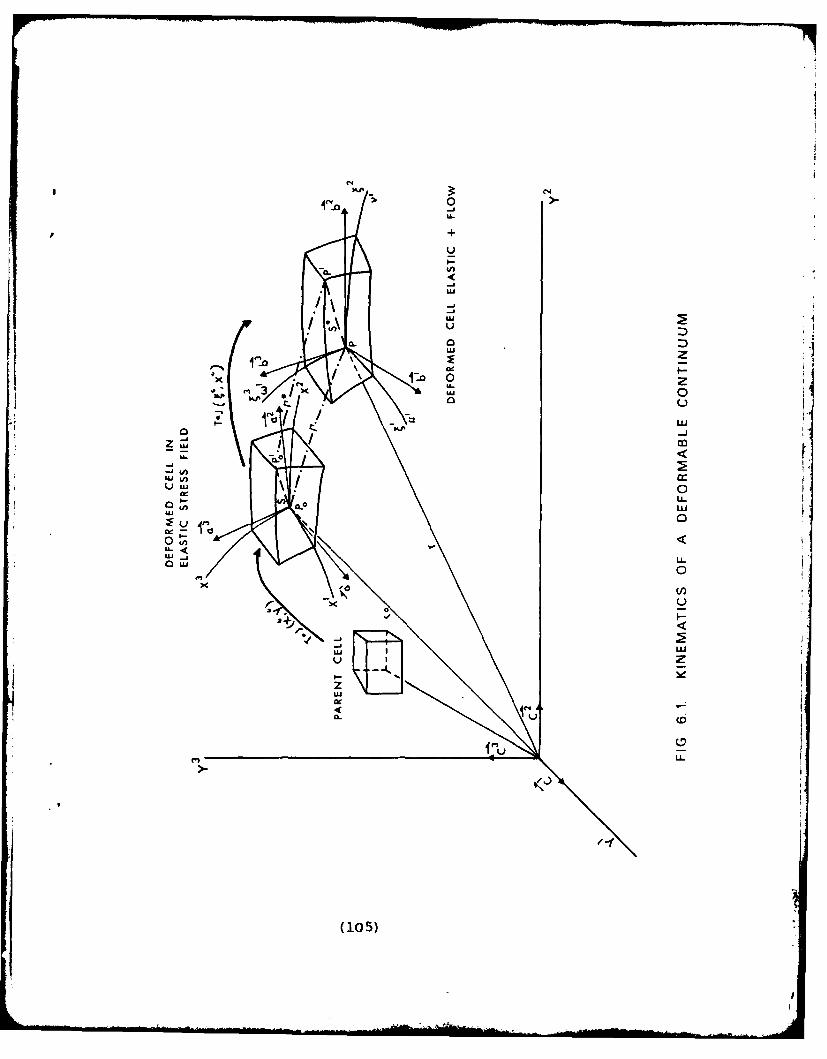
'.44

L.

+

LU

I-

u

LLU

00

UJ U)

Uu~ a

LU-

LL, -0

Oua 0

dww

:E -

(10X

0 U)

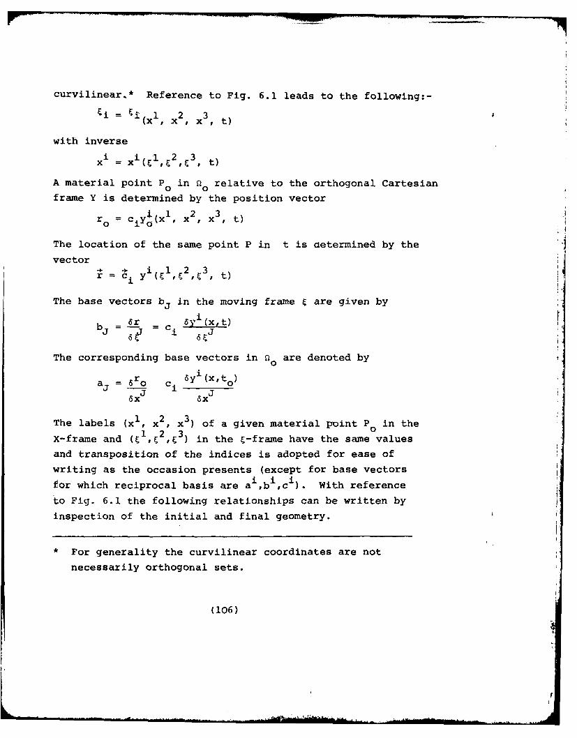
77 __

curvilinear.* Reference to Fig. 6.1 leads to the following:-

i = 1 , 2 x3(x 1 x 2 x 3 t)

with inverse

xi xi 2( 1 , E, t)

A material point P in Qo relative to the orthogonal Cartesianframe Y is determined by the position vector

r = ciY (xI, x2 , x3 , t)

The location of the same point P in t is determined by the

vector4- i 123r ci y (l, 2 ,1 3 t)

iiThe base vectors bj in the moving frame are given by

r c yi (x,t) Vbj se V = i 6 J6 J

The corresponding base vectors in £z are denoted by

aj = r ci y1 (Xto)xJ x JSx 6x

The labels (x1 , 2, x3 ) of a given material point P in the

X-frame and ( 1, 2,23) in the E-frame have the same valuesand transposition of the indices is adopted for ease of

writing as the occasion presents (except for base vectors

for which reciprocal basis are a i,b i,c i). With reference

to Fig. 6.1 the following relationships can be written by

inspection of the initial and final geometry.

* For generality the curvilinear coordinates are not

necessarily orthogonal sets.

(106)

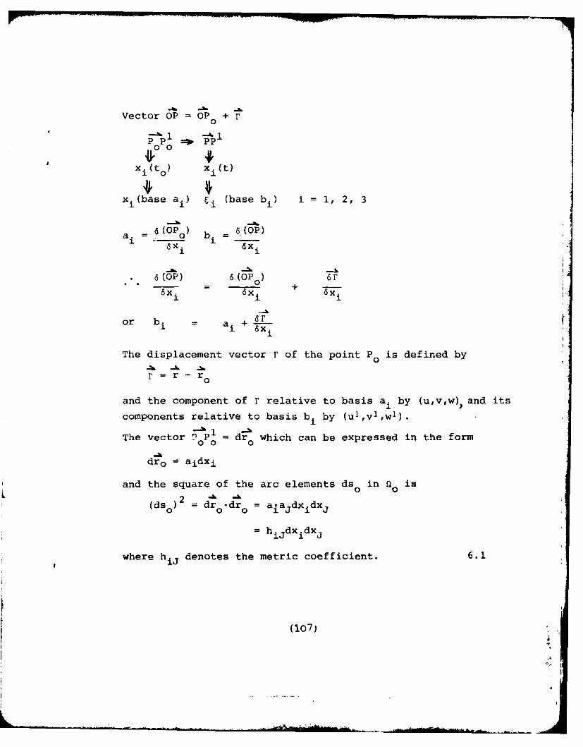
Vector OP = OP + r

~,ooP P =do PP

x i(to ) x i W

xi(base ai) Ei (base bi) i = 1, 2, 3

a. - (OPo) b. = 6 (OP) :- (5X

4 (op) 6(OP)

6( OP) 6(OP ) 6r

6x 6xi +

or bi = ai + 66xi

The displacement vector r of the point P is defined by

r = r - r

and the component of r relative to basis a. by (u,v,w) and its

components relative to basis b. by (ul ,vl ,w l).1

The vector .0P 0 = dr0 which can be expressed in the form

dro = aidxi

and the square of the arc elements ds in ao is

2 &- L i(ds 0 dr0 dro = alajdxidxJ

= hijdxidxJ

where hij denotes the metric coefficient. 6.1

(107)

I,

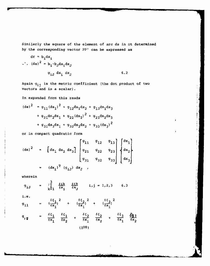
Similarly the square of the element of arc ds in Ot determined

by the corresponding vector PP' can be expressed as

dr = bidxi( )2

(ds)' bi.bjdxidxJ

giJ dxi dxj 6.2

Again gij is the metric coefficient (the dot product of two

vectors and is a scalar).

In expanded form this reads

2 2(ds) gll(dx) gl2dxdx2 + gl3 dx dx32 1 dx1 dx 1 2 131

22*+ g 2 2 (dx 2 ) + g2 3 dx 2 dx3

+ g31dx3dx 1 + g3 2dx 3dx 2 +33 3

or in compact quadratic form

g 1 1 g 12 g 1 3 dx1

(ds)2 [dx1 dx2 dx3] g21 g22 g23 1dx2

g3 1 g32 g33 dx3

- (dxi)T (gj) dx ,

wherein

3

k6 6X i,j = 1,2,3 6.3S 1 6x

i.e.2 2 6& 2

1 2 1 2 .x 1

(108)

6.5 Strain Rate

Finite strain is defined by one of the following:-

(a) Green's strain tensor

(b) Almansi's strain tensor

(c) Natural/logarithmic strain

The Green's tensor gives quadratic strains with respect to the

initial coordinates by the definition:-

jk ( xj bx k -- jk

= 1- )_6kk

r2 s 13) 6.4

dswhere 6 denotes the Kronecker delta and d- is the length

ratio of the line element initially parallel to the x 1-axis

which may have any current orientation.

The Almansi tensor reads:-6xk 6Xk 6.5

Jk Jk -6

Here ds is the length ratio of the element parallel to theHs-)current axis, which generally had some other orientation in

the initial state.

Thus the Green's strain tensor, which is the most commonly used

measure of finite strain, gives

(ds) 2 - (ds0 ) 2= 2 cij dx i dxj 6.6

Since (6.6) is an invariant and e i = ji the set of functions

Cij(x,t) represent a tensor L with respect to a class of

(109)

admissible transformation of coordinates X, with the basisai covering the region Qo The same set of functions

Eij( ,t) also determines a tensor E with respect to a set oftransformations of coordinates determined by the basis bi of

the final state Q. The first interpretation is termed

Lagrangian; it leads to expressions for the displacement

from the position xi in the undeformed state to the deformed

position Fi On the other hand the second interpretation,

the Eulerian system, leads to expressions for displacements

that must have taken place to get to the final position

from the undeformed configuration x.. The distinction between

lagrangian and eulerian variables becomes negligible for small

strains and rotations.

The set of differential equations for the components of the

displacement when the functions c are specified becomes

giJ - hij = 2 ij 2,ij 6.7

Therefore, from a purely geometrical standpoint, we may bring

a neighbourhood of P from its initial to its final state by

first translating the neighbourhood to move P to P, and then byo

rotating it so that orthogonal coordinate axes of the initial

state point in the orthogonal directions of the final state,

and finally deforming the neighbourhood by stretching the

three axes by the ratios of the current to the initial lengths

parallel to the initial axes. Hodge (1970) pp. 135-137.

Hence an arbitrary translation of a deforming element will

derive from two parts represented respectively by the strain

tensor J and a rotation tensor wiJ. The elements of the

strain tensor are, in a convenient notation, given by

(110)

.. . .. : : T, , ... . . .. . ., . .. .., , ..... . '

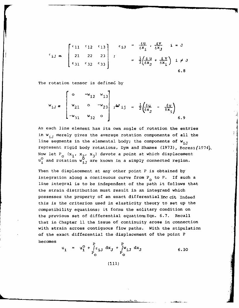
6 U, 6V i =Jll £12 E13 £iJ 6x1

6 xj

iJ jc21 22 23 ; i(6u ) v

E3 1 £32 E33 6.8-j 6x6.8

The rotation tensor is defined by

0 -w12 w13

wiJ= 21 w 2 3 ;L ij -u 6 v7 xj 6

-w31 w32 o 6.9

As each line element has its own angle of rotation the entries

in w merely gives the average rotation components of all the

line segments in the elemental body; the components of wij

represent rigid body rotations, Dym and Shames (1973), Boresi(1974).

Now let P0 (xI , x2, x3 ) devote a point at which displacement

u° and rotation w 0 are known in a simply connected region.

Then the displacement at any other point P is obtained by

integration along a continuous curve from P to P. If such a

line integral is to be independent of the path it follows that

the strain distribution must result in an integrand which

possesses the property of an exact differential IKDc cit Indeed

this is the criterion used in elasticity theory to set up the

compatibility equations; it forms the solitary condition on

the previous set of differential equationsEqn. 6.7. Recall

that in Chapter 11 the issue of continuity arose in connectionwith strain across contiguous flow paths. With the stipulation

of the exact differential the displacement of the point P

becomes

p p

0 i ) 0,

• "' ' , . .. . .. • "i , . .. i l l.)

where

E ik 6ii= 0xI

6xk

6Wik 6wil6x I

0

For the general case of an arbitrary integration path the dis-

placement field must be determined by integrating the rather

cumbersome integrands of Eqn.6-lOwith respect to non-rectilinear

coordinates. Fortunately the sets of equations 6.7 and 6.10

assume quite simple forms when an orthogonal curvilinear

system with origin on a flow line is chosen.* By setting a

principal coordinate direction tangential to the flow-line and

by making the flow line a path of integration the equation for

the displacements becomes (with reference to Fig. 6.1)

r ] t+At

u(t) u 0 + fiz(t)dr 6.11

where 1 1 (t) denotes the direct strain rate component as a

function of time of straining. On an axis of symmetry, or on

Along a flow line the following relationships hold:

1. rotations wij = 0 due to orthogonality of coordinate axes

2. metric coefficients reduce to gii' hii and the quadraticform becomes

(ds) 2 g2x ~ x 2 2(d)2= gll(dXl1) 2+ g 22 (dx 2) 2+ 933 (dx 3)2

i.e. g1 2 = g21 = alea 2 = 0 g3 1 = g1 3 = aloa 3 = 0

3. the displacements parallel to the flow lines are sufficientto plot a flow field. Transverse component perpendicularto flow line is determinate by property of exact differen-tial if required.

(112)

a rigid boundary u0 is zero; the value of ur represents the

4extension, or contraction, of a flow path relative to its

length at time t measured from a fixed datum, i.e. a symmetry

axis or rigid boundary.

Where the boundary itself is subject to displacements of

interest, as beneath a surface traction, the Equation 6.11

provides a relationship for incremental solution of the

points of the flow line with respect to the initial position.

The displacements at points along the flow line are further

governed by the Equation 2.10 and 2.11. (There is a direct

analogy here with the problem of a non-uniform variation of

temperature in a heated elastic solid; the strains at any

point is given by e = aT and these must be integrated with

respect to the coordinates to arrive at the displacements).

Evidently the evaluation of the displacements along individual

flow lines will yield the complete displacement field for

axially symmetric and plane strain problems. The displacements

so determined over incremental time steps, assuming a linear

variation over the duration of each time step, will sum to the

total displacements at any desired time t; i.e. the motioni i

between xn and xni is linear. As a consequence, the incre-i

i

mental velocity given by vn+ - Axi/At is constant over the

time increment. The author predicts that the application of

Eqn. 6.11 will give an enhanced insight into flow mechanisms

compared with solutions by the finite element or kernel

methods discussed earlier in this report.

(113)

-I

CHAPTER 7

INTERPRETATION OF CREEP TESTS AND

SUMMARY OF INVESTIGATION

7.1 The Theory of Creep Potential as an aid to Interpreta-tion of Experimental Data.

The theory of creep potential is based on concepts intro-

duced in plasticity theory for the purpose of evaluating

relative strain rates in ideal plastic solids. The

plastic potential function f(aij) is a scalar function of

stress which yields relative strain rates (the time variable

is a dummy term) according to the expression Drucker and

Prager (1952)

iJ= A cijiJ i 7.1

where A is a non negative constant. Extension of this

concept to creep leads to an analogous relationship Penny

and Marriott (1971).

de = d d7iJ 7.2

For isotropic materials the experimental evidence seems

to favour the von Mises criterion for formulation of creep

potential surfaces. In the case of isotropic multiaxial

creep the creep potential deduced from the criterion is

*2*(aij) 3-

Then the creep strain increments are related to the stress

components in the expression, loc cit.

(114)

3 ds 73ij,c 2 * ij 7.3

where Sij = 6/6a i. is termed the stress deviator. A

similar interpretation is employed in visco-plasticity

theory of Chapter I of this report. However, the application

of creep potential theory has not been extensive compared

with the hereditary integral theory or with the empirical

constitutive relationship approach.

The present author suggests that the concept of creep

potential deserves more attention than hitherto found in the

literature. It is one approach that promises to inject some

unification into the handling of experimental data. In order

to generalise, it is imperative that different stress states

can be taken into account and that no matter what is the

stress state in the material the interpretation of experi-

mental data leads to a unique value of the velocity at each

point in the body. To fix ideas consider the types of data

derived from the following set of laboratory tests:

1. uniaxial tension or compression on prismatic specimens

2. triaxial compression test on cylindrical specimens

3. hollow cylinder subjected to differential lateral

pressures

In uniaxial tension there is no variation in stress normal to

direction of flow hence the notion of creep dependence on

stress gradient is inapplicable. Similarly, in the triaxial

test the stress gradient between the symmetry axis and

boundary is not significant as demonstrated by finite elementanalysis; the axial stress is virtually constant over the

length of the specimen and radial and hoop stresses attain

approximately 0.005 per cent. of the axial component.

(115)

!i

A state of pure shear implies that normal stresses do notexist on the planes of maximum shear stress. On the other

hand the hollow cylinder test exhibits creep under theaction of stress gradient in the radial direction but thesum of the radial and hoop stresses is a constant value.In the light of the earlier discussion of stress state inthe axisymmetric flow of a semi-infinite medium caused bynormal stresses on a part of the boundary the hypothesisof normal stress gradient as the primary source of theforcing function appears to present just one further optionfor interpreting test data. The problem is how to assimi-late the results of different test configurations in aunified presentation. The earlier mentioned use ofeffective stress-strain is one such attempt at unificationas indeed the choice of constants makes the components

consistent for uniaxial and multiaxial tests.*

Again the stress components octohedral normal (aoct) andoctohedral shear (TOct) play a similar role as thesestress components are related to the stress invariantsand give a measure of the hydrostatic and the deviatoric

components of the state of stress at a point. Theserelations are

Oct = 2 +33

1 2 2 2 1/2toct =5{( l a2) +(2 -3) +(o3 - i

Effective stress in this context is not to be confusedwith the meaning of the word in Soil Mechanics litera-ture; perhaps the term 'equivalent stress' or 'generalisedstress woufd avoid the ambiguity.

(116)

Wi a

O2 - 1/2

Eoct = + 33

Y = - 2 ( - 27Oct f

+ ( - E) 2 7.4

The spatial derivative of -oct is taken as a measure of

the shearing intensity in a discretized zone according tothe foregoing hypothesis of normal stress gradient as the

forcing function. The hypotheses is merely a restatement

of the case for creep that the von Mises criterion in

plasticity theory may be extended to include dependence

on hydrostatic stress. The yield surface will generate

a circular cone symmetrical about the hydrostatic axis.

The extended von Mises criterion takes the form, Harr

(1966) pp 169

2 2 2 32(ol - 2 ) 2 + (2 -01) + (ol - 3 ) =k(ol + o2 + o

7.5

where k is a function of frictional resistance characterisedby the angle in granular media. The extended von Mises

criterion is treated in more detail by Nhdai (Vol. 1pp 226-228).

Stress Manifolds

From the foregoing discussion it follows that we seek a set

of functions in an n-dimensional stress space which has the

property of C1-continuity (at least in the domain of

interest). Mathematically the entity of the set is termed

a real analytic manifold; by definition it consists of n

functions of n variables which can be expanded in a

(117)

convergent Taylor series in a neighbourhood of each point,

Bruhat et al. (1977) pp 112. To be of value in the context

of integration for displacement fields the tangent planesto the manifold must give the strain rate in the directionof maximum velocity; ideally the dip of the tangent planeyields the maximum strain rate. The interpretation of testdata may thusly be reduced to forming the Sobolev space of

functions written symbolically as

WP (U) = F (aij'1 aj , ci1j,..., n=1,2,3,... 7.6

Some applications of this rather advanced topic infunctional analysis is covered in the Prentice-Hall CivilEngineering and Engineering Mechanics series, Oden 1979.Suffice it to say that the theory of topological spaces

provides a formalised approach to characterising a set of

functions and to investigating distributional partialderivatives of the set.

7.2 Summary

The study of creep undertaken in this report has examinedthe subject from a variety of standpoints. The firstchapter deals with the classical theories and serves asbackground to further development. As with works of anoriginal nature the outcome consists of a mixture of

disappointments and satisfaction. On the negative sidethe postulate of a transform for quantifying strain rateis defective in the sense that the answer depends on thediscretization of the solution domain, cf. Chapter 11.Another disappointing aspect emerges in Chapter 111 wherein

it is shown that only a limited set of flow patterns couldbe generated by the proposed harmonic analysis; the set

(118)

contains few patterns symmetric about the axis of

symmetry of a loaded area on a semi-infinite half space.

Apart from these findings positive contributions may be

claimed as follows:

1. A framework is established for predicting the dis-

placement field as a function of time of straining

provided that strain rates can be specified at sufficient

points in the solution domain.

2. The stress fields are determined by a summation

process in a simple algorithm.

3. The geometry of Laplacian flow nets is treated in

detail as are the different types of boundary condition.

4. Computer programs have been prepared for implementing

some of the analytical techniques.

5. The study culminates in the suggestion that functional

analysis offers an approach to a unified interpretation

of experimental data.

6. The main simplification results from the proposed method

of direct integration along flow paths. This innovation

allows a free choice of the strain rate tensor because

infinitesimal and finite strains can be handled with equal

ease in evaluating the line integral for displacement;

the strain rates are formulated as a part of the inter-

pretation of experimental data with no further implications

in the analytical technique.

(119)

REFERENCES

Adeyeri, J.B. and Krizek, R.J., "Mimic Source Approach to

Viscoelastic Analysis". Proc. ASCE Sym Application of

Finite Element Methods in Civil Engineering, Vanderbilt

University, 1969.

Ahlvin, R and Ulery, H.H., "Tabulated Vlaues for Determining

the Complete Pattern of Stresses, Strains and Deflections

beneath a Uniform Load on a Homogeneous Half-space".

H.R.B. Bull 342, 1962.

Al Salihi, M.Z., Parametric Surfaces in Finite Element

Analysis of Thin Shells. Ph.D. dissertation, University of

Dublin, 1978.

Arutyunyan, N.Kh., Some Problems in the Theory of Creep in

Concrete Structures. Pergamon Press, 1966.

Boresi, A.P. and Lynn, P.P., Elasticity in Engineerin

Mechanics, Prentice Hall, 1974.

Centurioni, L. and Viviani, A., "Contribution to Numerical

Computation of Laplacian Fields". Proc. X.E.E. Vol. 122 No 11

1975.

Courant, R. and Fritz John, Calculus and Analysis Vol II.

Chang Lu, P., Introduction to Mechanics of Viscous Fluids,Holt-Reinhart, Winston, 1973.

(120)

.!

Choquet-Bruchat, Y. Witt Morette, C.D. and Dillard-Bleick,

M., Analysis Manifolds and Physics, 1977.

Dewhurst, P. and Collins, I.F., "A Matrix Technique for

Constructing Slip-line Field Solutions to a Class of Plane

Strain Plasticity Problems". Int. Jour. for Numerical

Methods in Engineering Vol. 7, 1973.

Drucker, D.C. and Prager, W., "Soil Mechanics and Plastic

Analysis or Limit Design". Quart. Appl. Math. Vol 10 No 2,

1952.

Dym, C.L. and Shames, I.H., Solid Mechanics - A Variational

Approach. McGraw Hill, 1973.

Fenner, R.T., Finite Element Methods for Engineers,

Macmillan, 1975.

Ford, H. and Alexander, I.M., Advanced Mechanics of Materials

2nd. Ed. Ellis Horwood, 1976.

Frind, E.O., "An Isoparametric Hermitian Finite Element

for the Solution of Field Problems". Int. Jour. for

Numerical Methods in Engineering No 11, 1977.

Glen Murphy, Similitude in Engineering, Ronald Press Co. 1950.

Harr, M.E., Foundations of Theoretical Soil Mechanics.

McGraw Hill, 1966.

(121)

Henley, E.J. and Williams, R.A., Graph Theory in Modern

Engineering. Edited by R. Bellman, University of Southern

California, Academic Press, 1972.

Hildebrand, F.B., Advanced Calculus for Engineers.

Prentice - Hall Inc. 1957.

Hodge, P.G. Continuum Mechanics. McGraw Hill, 1970.

Huebner, K.H., Finite Element Methods for Engineers. Wiley,

1975.

Jumikis, A.F., Introduction to Theoretical Soil Mechanics.

Van Nostrand, 1967.

Key, S.W., Beisinger, Z.E. and Kreig, R.D. HONDO-11

A Finite Element Computer Program for the Large Deformation

Dynamic Response of Axisymmetric Solids. Sandia National

Laboratories, 1978.

Kuske, A. and Robertson, G. Photoelastic Stress Analysis.

Wiley Interscience, 1974.

Marsden, J.E., and Tromba, A.J., Vector Calculus. Freeman,

1975.

Mc Conologue, D.J., "A Quasi Intrensic Scheme for passinga Smooth Curve through a Discrete set of POints". Computer

Jour, No 13, 1970.

(122)

............

O'Laoide, B.O., Application of Potential Fields in Stress

Analysis, M.Sc. dissertation, University of Dublin, 1979.

Oden, J.T., Applied Functional Analysis. Prentice-Hall Inc.

1979.

Penny, R.K. and Marriott, D.L., Design for Creep. McGraw Hill

1971.

Rabotnov, Y.N. Some Problems of the Theory of Creep. 1953.

Sampine, X., and Allen, Y., Numerical Computing. W.B.Sanders

Co., 1973.

Shaug, J.G., and Bruch, J.C., "Seepage through a Homogeneous

Dam , Second Int. Sym. Finite Elements in Flow Problems".

ICCAD Santa Margherita Ligure Italy, 1976.

Sokolinikoff, I.S., Tensor Analysis. Wiley, 1964.

Thrower, E.N., "Methods for Predicting Deformation in Road

Pavements". Fourth Int. Conf. on the Structural Design of

Aspahlt Pavements Vol 1 Ann Arbor, 1977.

Timoshanko, S. and Goodier, J.N., Theory of Elasticity,

McGraw Hill, 1951.

(12 3)

__ . . . .. . . . . . . .. . . - , . . . . , "

Unksov, E.P., An Engineering Theory of Plasticity.

Butterworths, 1961.

Zienkiewicz, O.C. and Godbole, P.N., "Viscous Incompressible

Flow with Special Reference to Non-Newtonian Flow".

Finite Element in Fluids, Vol I, Wiley, 1975.

(124)

BIBLIOGRAPHY

Christian, J.T. and Watt, B.J., "Viscoelastic Analysis

of Soil Deformation" Proc. Sym. Applications of the Finite

Element Method in Geotechnical Engineering, Vicksburg,

Miss, 1972.

England, G.L., "The Direct Calculation of Stresses in

Creeping Concrete and Concrete Structures. Proc. Sym.

Stress Analysis, University of Southampton, 1969. *

Hu, S.T., Differential Manifolds. Holt Reinhart and Winston,

1969.

Leckie, F.A., "Structural Theorems of Creep and their

implications". Loc. cit.*

McConnell, A.J., Application of Tensor Analysis. Dover Press

1957.

Nadia, A. Theory of Flow and Fracture of Solids. Vols 1 and 2

McGraw Hill, 1963.

Paramichael, N and Whitman, J.R. "Cubic Spline Interpoldtion

of Harmonic Functions" B.I.T., Bind 14, Heffe NR4, 1974.

Sokolnikoff, I.S. and Redheffer, R.M. Mathematics and Physics

of Modern Engineering. McGraw Hill,1966.

(125)

.............................................

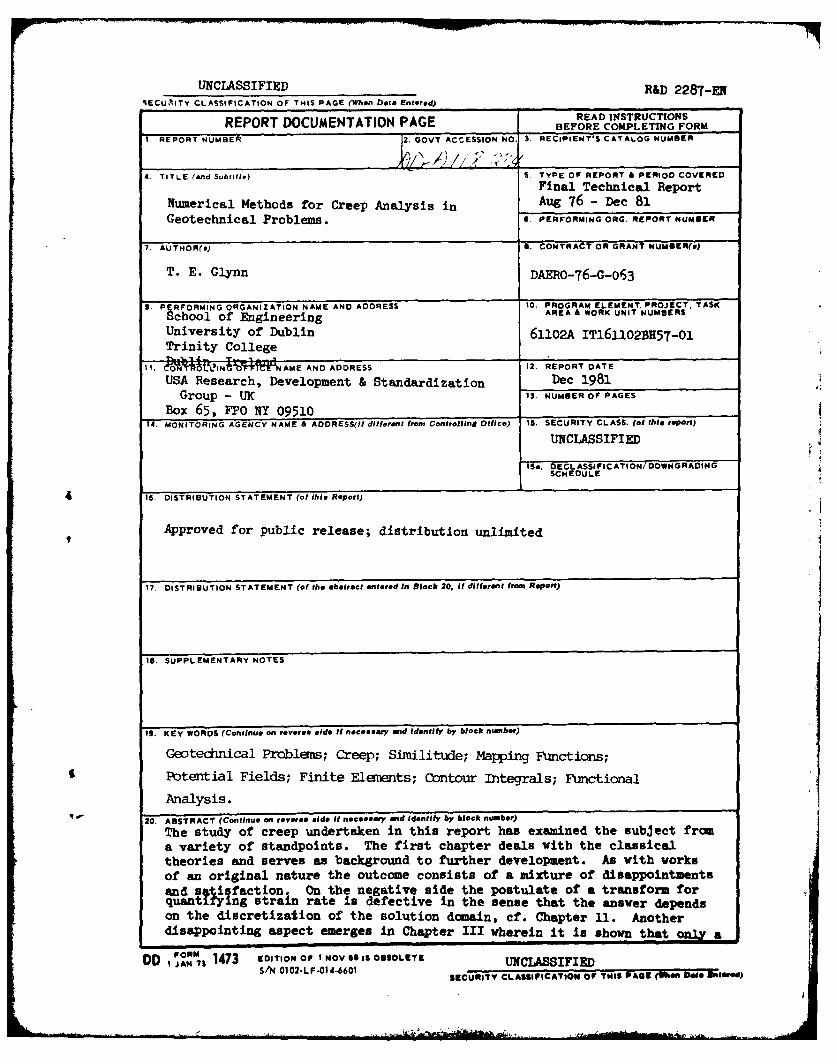
UNCLASSIFIED R&D 2287-EN;ECU'IUTY CLASSIFICATION OF THIS PAGE (When Dal Entered)

READ INSTRUCTIONSREPORT DOCUMENTATION PAGE BEFORE COMPLETING FORM

I. REPORT NUMBER 2. GOVT ACCESSION No. 3. RECIPIENT'S CATALOG NUMBER

4 TITLE (and Subtitle) S. TYPE OF REPORT & PERIOD COVEREDFinal Technical Report

Numerical Methods for Creep Analysis in Aug 76 - Dec 81Geotechnical Problems. 6. PERFORMING ORG. REPORT NUMBER

7. AUTHOR(s) S. CONTRACT OR GRANT NUMEeR(w)

T. E. Glynn DAERO-76-G-063

9. PERFORMING ORGANIZATION NAME AND ADDRESS I0. PROGRAM ELEMENT. PROJECT. TASK

School of Engineering AREA & WORK UNIT NUMBERS

University of Dublin 61102A IT161102BH57-0lTrinity College

It. I"tLINt' V;" NAME AND ADDRESS 12. REPORT DATEUSA Research, Development & Standardization Dec 1981

Group - UK 13. NUMBER OF PAGES

Box 65, FPO NY 0951014. MONITORING AGENCY NAME & ADDRESS(f dilletent from Controllinl Office) IS. SECURITY CLASS. (of this report)

UNCLASSIFIED

ISa. DECL ASSIFICATION/ DOWNGRADINGSCHEDULE

4 16. DISTRIBUTION STATEMENT (of $lis Report)

Approved for public release; distribution unlimited

17. DISTRIBUTION STATEMENT (of the abtract entered In Block 20, if different from Report)

Is. SUPPLEMENTARY NOTES

19. KEY WORDS (Continue on reveree side it neceeeary end Identify by block number)

Geotednical Problems; Creep; Similitude; Mapping Functions;

Potential Fields; Finite Elements; Contour Integrals; Functional

Analysis.

20. ABSTRACT (Continue on reveree side If neceeeary and Identify by block number)

The study of creep undertaken in this report has examined the subject froma variety of standpoints. The first chapter deals with the classicaltheories and serves as background to further development. As with worksof an original nature the outcome consists of a mixture of disappointmentsand satisfaction. On the negative side the postulate of a transform forquantifying strain rate is defective in the sense that the answer dependson the discretization of the solution domain, cf. Chapter 11. Anotherdisappointing aspect emerges in Chapter III wherein it is shown that only a

DD FORI. 1473 EDITION OF I NOV 55 IS OBSOLETE UNCLAS8IFIEDS/N 0102.LF.014-6601 SECURITY CLASSIFICATION OF TNIS P&OS (1li bale WweeJ)

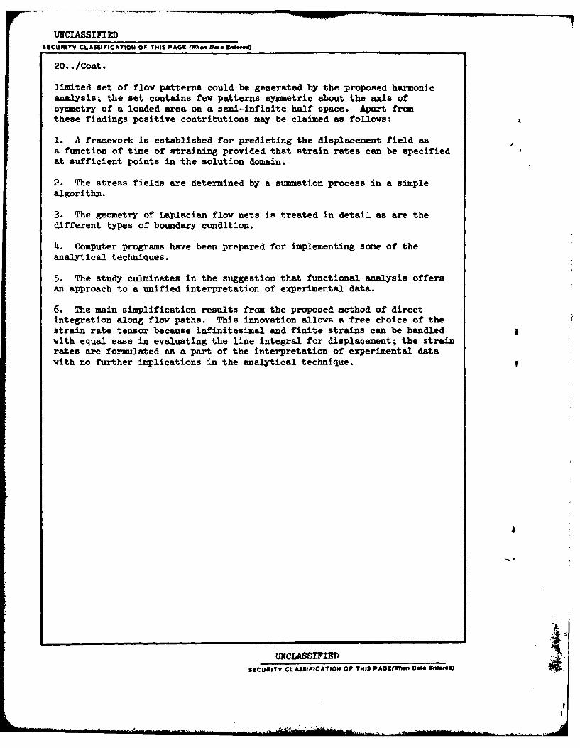
UNCLASSIFIEDSECURITY CLASSIFICATION OF THIS PAGE (hna, Do neaIe.,4

20. ./Cont.

limited set of flow patterns could be generated by the proposed harmonicanalysis; the set contains few patterns symmetric about the axis ofsymmetry of a loaded area on a semi-infinite half space. Apart fromthese findings positive contributions may be claimed as follows:

1. A framework is established for predicting the displacement field asa function of time of straining provided that strain rates can be specifiedat sufficient points in the solution domain.

2. The stress fields are determined by a summation process in a simplealgorithm.

3. The geometry of Laplacian flow nets is treated in detail as are thedifferent types of boundary condition.

4. Computer programs have been prepared for implementing some of theanalytical techniques.

5. The study culminates in the suggestion that functional analysis offersan approach to a unified interpretation of experimental data.

6. The main simplification results from the proposed method of directintegration along flow paths. This innovation allows a free choice of thestrain rate tensor because infinitesimal and finite strains can be handledwith equal ease in evaluating the line integral for displacement; the strainrates are formulated as a part of the interpretation of experimental datawith no further implications in the analytical technique.

UNCLASSIFIEDSECURITY CLASSIFICATION OF THIS PAOE(Wm

he Daa f 3uIw,.

I