DURABILITY-BASED DESIGN CRITERIA FOR A QUASI-ISOTROPIC CARBONFIBER AUTOMOTIVE COMPOSITE

J. M. Corum, R. L. Battiste, and M. B. Ruggles-WrennOak Ridge National Laboratory*

Oak Ridge, Tennessee 37831-8051

ABSTRACT

A major impediment to the increased application of composites for large structural automotivecomponents is the lack of design guidelines to assure the required 15-year durability. This paperdescribes the development of durability-based design criteria for a quasi-isotropic carbon-fibercomposite for possible automotive structural applications. The composite, which was made by arapid-molding process suitable for high-volume automotive applications, consisted of continuousThornel T300 fibers (6K tow) in a urea/urethane matrix. The reinforcement was in the form offour ±45E stitch-bonded mats in the following layup: [0/90/±45]S. In addition to elastic and creepproperties for design analyses, allowable time-dependent static stresses and allowable cyclicstresses are provided. Knockdown factors are incorporated to account for temperature effects andfor the degrading effects of exposure to fluid environments. Stress state and, in the case of cyclicloadings, mean stress effects are also incorporated into the criteria.

KEY WORDS: Composite Materials, Durability, Design Criteria

1. INTRODUCTION

The widespread use of composite systems to produce large structural automotive componentsrequires that their long-term durability be assured. An Oak Ridge National Laboratory (ORNL)project, sponsored by the U.S. Department of Energy and closely coordinated with theAutomotive Composites Consortium (ACC) is charged with developing the means for providingthis assurance. The approach is to develop experimentally based, durability-driven design criteriafor representative carbon-fiber-based composite systems. Durability issues being examinedinclude the potentially degrading effects of both sustained and cyclic loadings, exposure toautomotive fluids, temperature extremes, and low-energy impacts (for example, from tool dropsand kickups of roadway debris) and how they affect structural strength, stiffness, anddimensional stability.

*Oak Ridge National Laboratory, managed by UT-Battelle, LLC, for the U.S. Dept. of Energy under contractDE-AC05-00OR22725.

The project focus has been on the following progression of thermoset materials, all having thesame urethane matrix:

• reference [±45]3S crossply composite,• [0/90/±45]S quasi-isotropic composite, and• chopped-fiber composite.

Characterization of the first two systems has been completed and reported (1,2). The resultingdesign criteria for the quasi-isotropic composite is the subject of this paper. The chopped-fibercomposite is currently being characterized.

Both the crossply and the quasi-isotropic composites consisted of Thornel T300 continuousfibers (6K version) in a Baydur 420 IMR urethane matrix. The reinforcement was in the form of±45E stitch-bonded mats. Six mats were used in the 3.2-mm-thick crossply composite plaques.Four mats were used in the quasi-isotropic composite, which was 2.2 mm thick. The fiber-volume content was approximately 40% in both cases.

The 610- by 610-mm plaques were molded by ACC using an “Injection-CompressionProcedure.” For this process a preform is produced by assembling the required layup of ±45°mats and introducing them into a mold. The mold is left open approximately 10-15-mm. Thematrix is produced via the Structural Reaction Injection Molding (SRIM) process in which thetwo reactive systems, polyol and polymeric isocyanate, are pumped at high pressure into animpingement mixing chamber to quickly produce a uniform mixture of the components. Thereacting mixture is then pumped into the partially open mold that contains the reinforcement,after which the mold is fully closed. This allows the resin to first flow, with little resistance,across the upper surface of the preform and then, under increasing closing pressure, flow throughthe thickness of the preform. This procedure results in less disturbance of the fiber orientationand produces a more uniform, void-free, distribution of resin through the carbon-fiber preform.The time required for the liquid-to-solid transformation is of the order of 15-20 s. Final postcurewas 1 hour in a preheated oven at 130°C.

The average room temperature tensile properties of the quasi-isotropic composite are:• ultimate tensile strength, 336 MPa,• Young’s Modulus, 32.4 GPa, and• Failure ductility, 1.02%.

More than 1400 individual tests of laboratory specimens were performed to replicate on-roadconditions and to generate data to form the basis for developing correlations and models for thequasi-isotopic composite. These correlations and models were then used to formulate designcriteria. The types of tests included the following:

• basic short-time tension, compression, and shear;• uniaxial and biaxial flexure;• cyclic fatigue, including mean stress effects;• tensile and compressive creep and creep rupture;• tests of hole effects;*

• low-energy impact;* and• compression-after-impact.*

In most cases, characterization of the effects of temperature and fluid exposure was included inthe test effort. The specimen configurations and test methods were generally the same as thoseused previously to address the durability of glass-fiber composites (3).

Despite the relatively large number of tests performed, more extensive testing would be neededin several areas to provide sufficient data for developing completely defensible correlations,models, and design criteria. The approach taken here was to first perform as many carefullyplanned tests as possible within time and budget constraints. Then the design criteria weredeveloped with the philosophy of providing the best possible engineering design guidance giventhe limited information available. This sometimes required assumptions and extrapolationsbeyond the range of the existing data. Clearly, while the information in this paper should beadequate for preliminary designs undertaken with this material and for comparative purposeswith other materials, more information would likely be required for final design purposes.

For the design criteria, it was assumed that an automobile with a composite structure must lastfor 15 years (131,000 hours) and 150,000 miles. It was further assumed that during the 15 years,the vehicle will actually be operated about 5000 hours. The design temperature range was takento vary from a minimum of –40°C to a maximum of 120°C, with the higher temperaturesoccurring only during operation.

In addition to functional stiffness and deformation requirements, structures must support andresist a variety of live and dead loads. During operation, for example, live loads might include acombination of pothole impact, hard turn, and maximum acceleration. Dead loads during the15-year life would include those from the weight of the vehicle or sustained loads in the bed of alight truck.

Structures will also be exposed to common vehicle fluids and operating atmospheres, and designlimits must take the resulting property degradation into account. The effects of a variety of fluidsand moisture conditions were examined in the case of glass-fiber composites and in screeningtests on the crossply carbon-fiber composite. Based on the combined finding, the fluids mostextensively examined here were reduced primarily to distilled water and windshield washer fluid(a methanol/water mix).

The following three sections correspond to the three main parts of the design guidance:1) material properties for design analyses, 2) time-dependent allowable stresses for static loads,and 3) design rules for cyclic loads. In each case, the supporting data are described and designguidance is provided.

* Information from these test types was used in formulating damage tolerance assessment guidelines, which are notcovered in this paper.

2. ELASTIC AND CREEP PROPERTIES FOR DESIGN ANALYSES

It is presumed that design of automotive structural components will primarily employ linear-elastic finite-element plate and shell analyses, which are based on the material beinghomogeneous and isotropic. In addition to deformations, these analyses provide normalmembrane and bending stresses plus shear in the relatively thin molded sections envisioned forautomotive structures. Thus, elastic constants are required for analysis. Also, a means for at leastapproximately accounting for time-dependent creep is required. The necessary properties fordoing this are presented in this section.

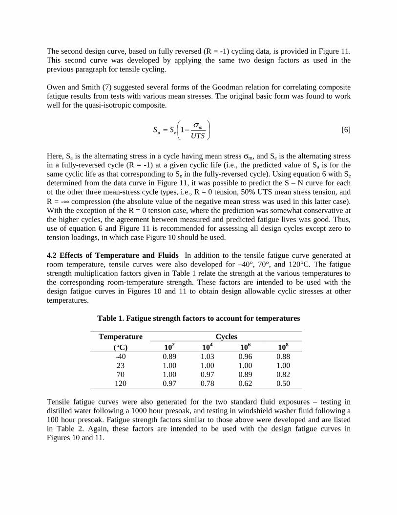
2.1 Elastic Constants It is shown in reference (2) that, except at higher temperatures andstresses, the quasi-isotropic composite is isotropic in the plane of the plaque.* For such ananisotropic layup that exhibits in-plane isotropy, the linear elastic response to in-plane appliedloads is characterized by two constants, E and G, or alternatively, E and ν, where E and G are theYoung’s and shear moduli, and ν is Poisson's ratio. The constants are related by the followingequation:

. [1]

Elastic property data from tensile tests and Iosipescu shear tests on V-notch beams confirm thatequation 1 is valid for the quasi-isotropic composite over the entire temperature range from –40°to 120°C.

Figure 1 shows the variation of Young’s modulus with temperature. Measured Poisson’s ratiovalues are also shown at specific temperatures.

Elastic properties are affected by prior cyclic loadings and, to a lesser extent, by exposure tofluids and to high humidity levels. These effects should be accounted for as appropriate. It wasfound that, repeated temperature cycling (26 cycles) from –40° to 120°C had no effect on tensileand compressive stiffness, but shear modulus was reduced by 25%. Prior load cycling cansubstantially reduce Young’s modulus. The fatigue limits presented in Section 4 were chosen, inpart, to assure that the stiffness loss does not exceed 10%. Finally, long-term exposure (up to5000 hours) in distilled water and 70% relative humidity (RH) and in windshield washer fluid(70% methanol/30% distilled water) led to stiffness reductions of at most 4%.

2.2 Creep Properties Long-term tensile creep tests were performed at room-temperature and at70° and 120°C, as well as in distilled water and in windshield washer fluid. The latter tests (seeFigure 2) were conducted after standard pre-exposures of 1000 hours in the case of distilledwater and 100 hours in the case of windshield washer fluid.

The following empirical equation was developed for describing time-dependent creep strain atroom temperature.

* At temperatures above 100°C and stresses greater than 140 MPa, the normally linear stress-strain responsebecomes slightly nonlinear, and this non-linearity is most pronounced at loading angles, like 22.5°, between fiberorientations.

( )ν+=

12E

G

[2]where

A = 7.268 x 10-10 σ3 + 2.614 x 10-8 σ2

+ 2.789 x 10-5 σ + 2.960 x 10-5

n = 4.662 x 10-7 σ2 – 2.587 x 10-4 σ+ 0.2540 .

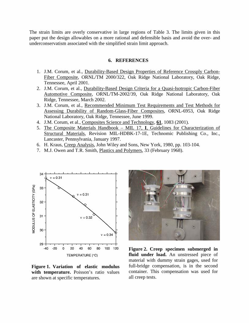
The predictions of equation 1 are compared in Figure 3 with the results of several long-termcreep tests. The agreement is good at the lower stresses. Localized damage accumulation at thehigher stress levels led to increased data scatter, but on average, the agreement is reasonable.

The effect of increasing temperature on time-dependent creep strain can be accounted for bymultiplying the strains predicted by equation 2 by a factor, which is plotted in Figure 4. For fluideffects, the results of tests performed under the two standard exposures, mentioned above, led tocreep multiplication factors of 1.7 for distilled water and 1.5 for windshield washer fluid.

Creep under compressive stresses is much more matrix-dominated, and, at least at highertemperatures and stress levels, is likely to involve some local buckling. Limited compressivecreep data indicate that at room temperature, compressive creep is the same as tensile creep.However, at 120°C, compressive creep appears to be much larger than tensile creep, and thefactor, rather than being constant as in the tensile case, depends on stress level. Factors as high as77 times the room-temperature tensile creep were found. Clearly long-term compressive loadingsshould be avoided at 120°C.

3. ALLOWABLE STRESSES FOR STATIC LOADINGS

The basic allowable stresses used in this section are time-dependent. They are derived from bothinstantaneous and creep-rupture tests. The system of allowable stresses used here follows thatdeveloped earlier for random-glass-fiber composites (4).

3.1 Short-Time Allowable Tensile Stress, S0 The basic short-time, or instantaneous, allowablestress is based on the minimum room-temperature ultimate tensile strength (UTS), which isdefined as the “B-basic stress” (5). The minimum room-temperature value is based on statisticaltreatment of n = 86 UTS values, such that the survival probability at the minimum stress is 90%at a confidence level of 95%. This minimum value was calculated to be 291 MPa. The allowablestress, S0, is defined as two-thirds UTSmin. At room-temperature, S0 thus becomes 194 MPa,which is 58% of the average UTS. Values of S0 at other than room temperature were obtained bymultiplying the room-temperature value by the ratio of the average at-temperature UTS to theroom-temperature UTS.

The UTS, and hence S0, can be reduced by several other effects. First a sequence of priorloading/unloading steps to 20%, 40%, 60%, and 80% of the average UTS was found to reduce

nc At=ε

the subsequent UTS by 15%. While 80% UTS is significantly above S0, a single prior loading to80% UTS alone reduced the subsequent UTS by just 6%, so the lower stresses had a majoreffect. Thus, prior load effects should at least be considered in design. Second, prior thermalcycling between –40°C and 120°C reduced the subsequent UTS by almost 7%. Finally, while thestandard fluid exposures did not reduce the UTS, exposure to humid air (70% RH) did. Areduction of almost 6% bounds the latter effect for exposure times up to almost 5000 hours. If allthese reductions were applied simultaneously, the assumed effect on S0 would be

S0 = (0.85) (0.93) (0.94) 194 = 144 MPa

Ultimately the designer must judge which factors are appropriate for the application.

3.2 Time-Dependent Allowable Tensile Stress, St For sustained loadings, creep-rupture stressis the basis for time-dependent allowable stresses, provided that S0 is not lower than the creep-derived values. For uniaxial tension the time-dependent allowable stress, St, is defined as

≤r

t S

SS

8.00 [3]

where Sr is the minimum creep-rupture strength. Note that St=S0 at zero time.

The creep-rupture curves from which Sr was determined are shown in Figure 5. Because of thepaucity of failure data, the “minimum” curves were established by simply shifting the originalaverage curves down to bound all of the data points.

The Manson-Haferd time-temperature parameter was used to generate Sr values at other thanroom temperature and 120°C. Details of the use of the Manson-Haferd parameter can be found inreference (6). The parameter is expressed as

[4]

where T is temperature in degrees Rankin, and tr is rupture time in hours. The constants Ta and ta

are determined by the interaction point of lines representing the available data at various stresslevels on a plot of T vs log10 tr. The solid line in Figure 6 shows the resulting plot of tensile stressvs the Manson-Haferd parameter. Note that in this plot T is in °C. Creep-rupture stresses forvarious times at several specific temperatures were determined from the master curve and used,in turn, to determine reduction ratios of the stresses at each temperature relative to those at roomtemperature.

Values of St without environmental or prior load effects are plotted in Figure 7(a), where both S0

and 0.8 Sr are shown. Only at the longer times and higher temperatures do the 0.8 Sr values dropbelow S0. Figure 7(b) includes the effects of moisture/fluids on the allowables. The short-time S0

value includes the 6% reduction due to exposure in a 70% RH air environment. For creep-rupture, curves similar to those in Figure 5 were developed for the two standard fluid exposures.Windshield washer fluid had the greatest effect; reductions ranged from 3% at 10 hours to 6% at131,000 h (15 years). These reductions are included in the 0.8 Sr curves.

ar

aMH tt

TTP

1010 loglog)(

−−

=σ

3.3 Compressive and Biaxial Allowable Stress, St* To this point, the allowable stresses are

based on, and thus only apply to, uniaxial tensile stress states. In design, where other stress stateswill likely exist, a simple biaxial strength criterion is needed. Because the current composite isisotropic in the plane of the material, a simple criterion is possible.

The available average strength data at room-temperature, though limited, are plotted in principalstress space in Figure 8, where they are compared with common biaxial strength theories. Thesolid points in the figure are from the basic tensile, compressive, and shear test results. The open-point compressive strength values come from tests of a “compression-after-impact” typespecimen, which has antibuckling face-support plates. It is believed that the open points are amore accurate representation of the true compressive strength. Nonetheless, it was conservativeto use the solid compressive and shear points, even though both may reflect the influence ofbuckling of the thin specimens. The tensile and open compression points are consistent with anyof the criteria. However, the solid compression and shear points would dictate that the maximumstress theory is the best choice. Thus, it was adopted for evaluation of nontensile stress states.

Because temperature has essentially the same relative effect on both compressive and shearstrengths, the maximum stress theory should be applicable at any temperature. Furthermore,fluids have a larger effect on compressive strength than on shear strength, so the maximum stresstheory with the stress limited to the compressive strength, reduced by fluid effects, isconservative. For creep rupture, there are no available shear results, so the assumption must bemade that the compressive results with the maximum stress strength criterion are still adequate.

Only two compressive creep-rupture test results, both at 120°C, were available. To estimate afull set of creep-rupture results, use was again made of the Manson-Haferd parameter. It wasassumed that the tensile parameter also applies to compressive creep rupture, and the twocompressive data points were plotted on Figure 6. The master curve shown for compression inFigure 6 has a much more tenuous basis than that for tension. In addition to assuming that thetensile constants are applicable to compression, it was assumed that the two master curves wouldbe roughly parallel and that at large negative values of PMH, the stress is limited by the ultimatecompressive strength at room temperature – 225 MPa. With these assumptions, the curve wasdrawn.

The resulting allowable St* stresses, without environmental or prior load effects, are plotted in

Figure 9(a). Figure 9(b) depicts the values with estimated fluid effects included. Recall that anexposure to 70% RH air had the greatest impact on tensile strength – a reduction of 6%. Thatcondition was not evaluated for compression, but of the two standard fluid exposures – distilledwater and windshield washer fluid – distilled water had the greatest effect, and the reductionfactor was also 6%. This reduction is the basis for the S0

* curve in Figure 9(b). No compressivecreep-rupture tests in fluids were performed, so the reduction factors used for tension were alsoused for the 0.8Sr

* values in Figure 9(b). Note that S* is lower than the tensile allowable stress.

3.4 Treatment of membrane and Bending Stresses The St and St* values establish limits on

allowable in-plane membrane stresses, P. For out-of-plane bending away from structuraldiscontinuities, the combined membrane plus bending stresses, P + Q, are limited to

( )*tt SorKSQP ≤+ [5]

where K is 1.5 at –40° and 23°C, 1.3 at 70°C, and 0.9 at 120°C. These factors were derived fromshort-time beam flexure test results. It should be emphasized that equation 5 applies to bendingstresses elastically calculated assuming an isotropic, homogeneous material. Also equation 5does not apply to locations with geometric discontinuities (e.g., corners and bends). At suchlocations new failure modes can occur.

4. LIMITS FOR CYCLIC LOADINGS

Several series of fatigue tests were performed to provide a basis for design rules. Most of thetests were tension-tension fatigue, having a ratio, R, of minimum to maximum cyclic stress of0.1. These tension-tension tests were used to generate S – N (stress vs cycles to failure) curves atvarious temperatures and for specimens exposed to the reference fluids.

In addition to the R = 0.1 tension-tension tests, mean stress tests involving four different cycletypes were performed in air at room temperature. The cycle types were:

• R = 0 tension (zero to maximum stress),• R = -∞ compression (zero to maximum compressive stress),• R = -1 completely revered tension/compression, and• tensile tests with a mean stress equal to 50% of the UTS.

While the standard dogbone-shaped tensile specimen was used for the R = 0.1 tensile tests, anhourglass-shaped specimen was used for the mean stress tests to minimize buckling undercompressive loading.

4.1 Basic Fatigue Design Curves Two room-temperature, ambient-air design fatigue curves areprovided. The first applies to cycles in which the stress varies from zero to a maximum tensilevalue (R = 0). The second curve applies to fully reversed cycles (R = -1), where the stress variesfrom a tensile stress to an equal, but opposite, compressive stress. This latter curve may be usedwith the Goodman relation to determine the allowable lives for cycles with other tensile orcompressive mean stress values.

The tensile design curve, and its basis, is shown in Figure 10. Although the curve is intended toapply to R = 0 cycles, it is actually derived from R = 0.1 tensile cycling data. Comparative testsshow that there is little difference in results from the two cycle types.* Two margins were usedto derive the design curve. First, a margin of 20 was placed on cycles to failure. This assures thatloss of stiffness, which was monitored during each fatigue test, does not exceed 10%. Second, anadditional multiplication factor of UTSmin/UTSavg = 0.90 was applied to stress to obtain the finaldesign curve. This latter factor was judged to be necessary because of the significant scatter infatigue life.

* R = 0.1 is used simply to avoid the risk of subjecting the slender tensile fatigue specimen to a compressive loading.

The second design curve, based on fully reversed (R = -1) cycling data, is provided in Figure 11.This second curve was developed by applying the same two design factors as used in theprevious paragraph for tensile cycling.

Owen and Smith (7) suggested several forms of the Goodman relation for correlating compositefatigue results from tests with various mean stresses. The original basic form was found to workwell for the quasi-isotropic composite.

−=

UTSSS m

ea

σ1 [6]

Here, Sa is the alternating stress in a cycle having mean stress σm, and Se is the alternating stressin a fully-reversed cycle (R = -1) at a given cyclic life (i.e., the predicted value of Sa is for thesame cyclic life as that corresponding to Se in the fully-reversed cycle). Using equation 6 with Se

determined from the data curve in Figure 11, it was possible to predict the S – N curve for eachof the other three mean-stress cycle types, i.e., R = 0 tension, 50% UTS mean stress tension, andR = -∞ compression (the absolute value of the negative mean stress was used in this latter case).With the exception of the R = 0 tension case, where the prediction was somewhat conservative atthe higher cycles, the agreement between measured and predicted fatigue lives was good. Thus,use of equation 6 and Figure 11 is recommended for assessing all design cycles except zero totension loadings, in which case Figure 10 should be used.

4.2 Effects of Temperature and Fluids In addition to the tensile fatigue curve generated atroom temperature, tensile curves were also developed for –40°, 70°, and 120°C. The fatiguestrength multiplication factors given in Table 1 relate the strength at the various temperatures tothe corresponding room-temperature strength. These factors are intended to be used with thedesign fatigue curves in Figures 10 and 11 to obtain design allowable cyclic stresses at othertemperatures.

Table 1. Fatigue strength factors to account for temperatures

Temperature Cycles(°C) 102 104 106 108

-40 0.89 1.03 0.96 0.8823 1.00 1.00 1.00 1.0070 1.00 0.97 0.89 0.82120 0.97 0.78 0.62 0.50

Tensile fatigue curves were also generated for the two standard fluid exposures – testing indistilled water following a 1000 hour presoak, and testing in windshield washer fluid following a100 hour presoak. Fatigue strength factors similar to those above were developed and are listedin Table 2. Again, these factors are intended to be used with the design fatigue curves inFigures 10 and 11.

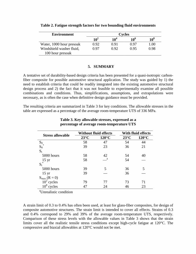
Table 2. Fatigue strength factors for two bounding fluid environments

CyclesEnvironment102 104 106 108

Water, 1000 hour presoak 0.92 0.91 0.97 1.00Windshield washer fluid, 0.97 0.92 0.95 0.98

100 hour presoak

5. SUMMARY

A tentative set of durability-based design criteria has been presented for a quasi-isotropic carbon-fiber composite for possible automotive structural application. The study was guided by 1) theneed to establish criteria that could be readily integrated into the existing automotive structuraldesign process and 2) the fact that it was not feasible to experimentally examine all possiblecombinations and conditions. Thus, simplifications, assumptions, and extrapolations werenecessary, as is often the case when definitive design guidance must be provided.

The resulting criteria are summarized in Table 3 for key conditions. The allowable stresses in thetable are expressed as a percentage of the average room-temperature UTS of 336 MPa.

Table 3. Key allowable stresses, expressed as apercentage of average room-temperature UTS

Without fluid effects With fluid effectsStress allowable23°C 120°C 23°C 120°C

S0 58 47 54 44S0

* 39 23 36 21St

5000 hours15 yr

5858

42—a

5454

40—

St*

5000 hours15 yr

3939

5—

3636

5—

Smax (R = 0)102 cycles108 cycles

7947

7724

7346

7123

aUnrealistic condition

A strain limit of 0.3 to 0.4% has often been used, at least for glass-fiber composites, for design ofcomposite automotive structures. The strain limit is intended to cover all effects. Strains of 0.3and 0.4% correspond to 29% and 39% of the average room-temperature UTS, respectively.Comparison of these stress levels with the allowable values in Table 3 shows that the strainlimits cover all the realistic tensile stress conditions except high-cycle fatigue at 120°C. Thecompressive and biaxial allowables at 120°C would not be met.

The strain limits are overly conservative in large regions of Table 3. The limits given in thispaper put the design allowables on a more rational and defensible basis and avoid the over- andunderconservatism associated with the simplified strain limit approach.

6. REFERENCES

1. J.M. Corum, et al., Durability-Based Design Properties of Reference Crossply Carbon-Fiber Composite, ORNL/TM 2000/322, Oak Ridge National Laboratory, Oak Ridge,Tennessee, April 2001.

2. J.M. Corum, et al., Durability-Based Design Criteria for a Quasi-Isotropic Carbon-FiberAutomotive Composite, ORNL/TM-2002/39, Oak Ridge National Laboratory, OakRidge, Tennessee, March 2002.

3. J.M. Corum, et al., Recommended Minimum Test Requirements and Test Methods forAssessing Durability of Random-Glass-Fiber Composites, ORNL-6953, Oak RidgeNational Laboratory, Oak Ridge, Tennessee, June 1999.

4. J.M. Corum, et al., Composites Science and Technology, 61, 1083 (2001).5. The Composite Materials Handbook – MIL 17, I, Guidelines for Characterization of

Structural Materials, Revision MIL-HDBK-17-1E, Technomic Publishing Co., Inc.,Lancaster, Pennsylvania, January 1997.

6. H. Kraus, Creep Analysis, John Wiley and Sons, New York, 1980, pp. 103-104.7. M.J. Owen and T.R. Smith, Plastics and Polymers, 33 (February 1968).

Figure 1. Variation of elastic moduluswith temperature. Poisson’s ratio valuesare shown at specific temperatures.

Figure 2. Creep specimen submerged influid under load. An unstressed piece ofmaterial with dummy strain gages, used forfull-bridge compensation, is in the secondcontainer. This compensation was used forall creep tests.

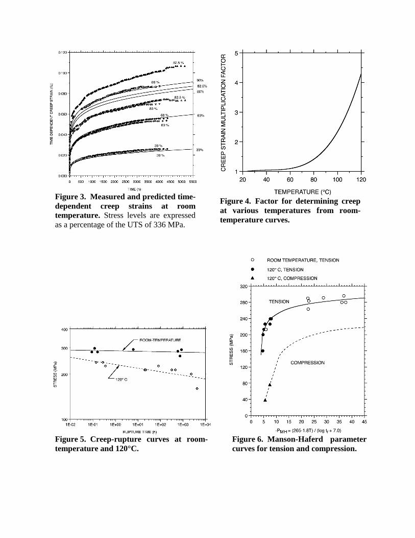
Figure 3. Measured and predicted time-dependent creep strains at roomtemperature. Stress levels are expressedas a percentage of the UTS of 336 MPa.

Figure 4. Factor for determining creepat various temperatures from room-temperature curves.

Figure 5. Creep-rupture curves at room-temperature and 120°C.

Figure 6. Manson-Haferd parametercurves for tension and compression.

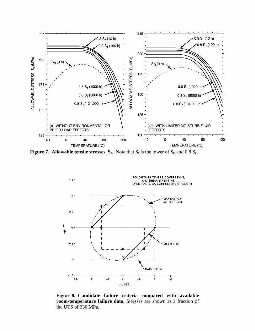
Figure 7. Allowable tensile stresses, St. Note that St is the lower of S0 and 0.8 Sr.

�

Figure 8. Candidate failure criteria compared with availableroom-temperature failure data. Stresses are shown as a fraction ofthe UTS of 336 MPa.

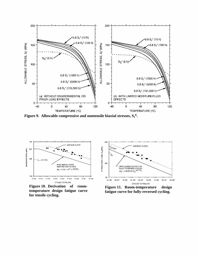
Figure 9. Allowable compressive and nontensile biaxial stresses, St*.

Figure 10. Derivation of room-temperature design fatigue curvefor tensile cycling.

Figure 11. Room-temperature designfatigue curve for fully-reversed cycling.