durham e-theses structure of amphiphilic block copolymer...
TRANSCRIPT
Durham E-Theses
Structure of amphiphilic block copolymer micelles in
aqueous dispersions
Leslie, Stuart
How to cite:
Leslie, Stuart (2003) Structure of amphiphilic block copolymer micelles in aqueous dispersions, Durhamtheses, Durham University. Available at Durham E-Theses Online: http://etheses.dur.ac.uk/3738/
Use policy
The full-text may be used and/or reproduced, and given to third parties in any format or medium, without prior permission orcharge, for personal research or study, educational, or not-for-pro�t purposes provided that:
• a full bibliographic reference is made to the original source
• a link is made to the metadata record in Durham E-Theses
• the full-text is not changed in any way
The full-text must not be sold in any format or medium without the formal permission of the copyright holders.
Please consult the full Durham E-Theses policy for further details.
Academic Support O�ce, Durham University, University O�ce, Old Elvet, Durham DH1 3HPe-mail: [email protected] Tel: +44 0191 334 6107
http://etheses.dur.ac.uk
Structure of Amphiphilic Block Copolymer Micelles in Aqueous
Dispersions
2003
S tu art Lesl ie
Graduate Society
University of Durham
Supervisor:
Professor Randal W Richards A copyright of this thesis rests with the author. No quotation from it should be published without his prior written consent and information derived from it should be acknowledged.
A thesis submitted to the University of Durham in partial fulfilment
of the regulations for the degree of Doctor of Philosophy.
1 9 JAN 2004

Abstract
Abstract
Structure of Amphiphilic Block Copolymer Micelles in Aqueous Dispersions
Stuart Leslie
PhD Thesis University of Durham 2003
Two molecular weight series of Poly(butadiene)-Poly(ethylene oxide) diblock
copolymers have been synthesised using anionic polymerisation techniques.
The amphiphilic nature of the copolymers results in micelles being formed on
dispersion in water. Dynamic light scattering was employed to ascertain the
critical micelle concentration and micelle dimensions. Small-angle X-ray and
neutron scattering were used to investigate high concentration dispersions
providing micelle dimensions and an insight into the nature of the interactions
between micelles from the structure factor, which develops at higher
concentrations. The detailed model used polymer brush theory to fit the
small-angle scattering data at low concentrations in the absence of
interparticle interactions. Micelle dimensions determined by model fitting
matched well with those predicted from theory. At higher concentrations
when these interactions are dominant, a Yukawa potential between micelles
was used to model the observed structure factor.
The unsaturation of the poly(butadiene) chains comprising the core of the
micelle facilitated post-polymerisation cross-linking of the core using a redox
initiated free-radical polymerisation at room temperature. Dynamic light
scattering was employed to determine the micelle dimensions, with small
angle X-ray and neutron scattering used to investigate higher concentration
dispersions. The micelle cores were seen to contract by circa 10-40% upon
cross-linking in relation to the virgin micelles, resulting in the junction points
of the coronal chains on the surface of the micelle core coming closer
together. Interestingly the thickness of the corona decreased in relation to
the virgin micelles, a phenomenon due to the presence of inorganic ions from
the cross-linking reaction reducing the thermodynamic quality of the solvent
for the poly( ethylene oxide) brush, causing it to partially collapse.
Acknowledgements
Acknowledgements
Firstly, I would like to thank my supervisor Professor Randal Richards for
providing me with the opportunity to carry out this research and for his
support and encouragement during it. Special thanks also go to Or Nigel
Clarke for his assistance and constructive comments following the departure
of Professor Richards.
None of this work would have been possible without the guidance of many
people, to whom I am greatly indebted. At Durham, Dr. lian Hutchings for
constructive disc~ssions about the synthetic chemistry, Dr. Zaijun Lu for
supplying the deuterated poly(butadiene), Doug for SEC, DSC and general
encouragement, Alan, lan and Catherine for NMR spectra, Jean, Anne and
lrene for sorting out my various travel arrangements, Malcolm and Peter for
constantly repairing the stream of broken glass and keeping ·me out of
trouble! At Rutherford Appleton Laboratory, Steve King for help with the
neutron scattering experiments and Richard Heenan for assistance with the
data fitting and the use of his FISH analysis software. At Sheffield, Or Patrick
Fairclough for the use of his light scattering apparatus.
My time in Durham has been an interesting one and I would like to thank all
members of the IRC both past and present, of which there are too many to
mention, with whom I have had the pleasure of working alongside, the
occupants of lab 1, and Gradsoc AFC.
I would like to thank my wife Wendy for putting up with me and for her love,
support and encouragement. Without you none of this would have been
possible, and my sanity would have suffered far more than it hast
Finally I would like to thank my parents and sister Donna for their love and
support.
ii
Declaration and Copyright
Declaration
The work reported in this thesis has been carried out at the Durham site of
the Interdisciplinary Research Centre in Polymer Science and Technology, the
Department of Chemistry, University of Sheffield and the Rutherford Appleton
Laboratory, Chilton, Oxfordshire between October 2000 and September 2003.
This work has not been submitted for any other degree either in Durham or
elsewhere and is the original work of the author except where otherwise
stated.
Statement of Copyright
The copyright of this thesis rests with the author. No quotation from it should
be published without prior written consent and any information derived from
it should be acknowledged.
Financial Support
The author gratefully acknowledges the provision of a maintenance grant by
the EPSRC.
iii
Abstract
Acknowledgments
Declaration
Statement of Copyright
Financial Support
Contents
1. INTRODUCTION
1. 1. Introduction
1 . 1 . 1 . Architecture
1.1.2. Nomenclature
1.1.3. Copolymer synthesis
1. 2. Micellisation
Contents
1.2.1. Theoretical description of micellisation
1.2.1.1.
1.2.1.2.
Scaling theories .
Self-consistent field theories
Contents
ii
iii
iii
iii
iv
1
2
3
4
4
6
8
8
12
1. 3. Polymer Brushes 14
1.4. Micellar behaviour of poly(butadiene)-poly(ethylene oxide) 19
1.4.1. Investigations of the Bates group 19
1.4.2. Investigations by other researchers 25
1.5. Micellar behaviour of poly(butylene oxide)-poly(ethylene oxide) 27
1.6. Micellar behaviour of poly(propylene oxide)-poly(ethylene oxide) 29
1. 7. Cross-linked micelles 30
1.7.1. Core cross-linked micelles
1.7.2. Shell cross-linked micelles
1.8. Aims and objectives
1. 9. Glossary of symbols
1. 9.1. Micellisation
1. 9.2. Polymer Brushes
1.1 0. Bibliography
31
34
36
37
37
37
38
iv
2. SYNTHESIS AND EXPERIMENTAL METHODS
2. 1 . Synthetic background
2. 1.1. Anionic Polymerisation
2.1.2. Why Use Anionic Polymerisation?
2.1.2.1. Molecular weight
2.1.2.2. Molecular weight distribution
2.1.2.3. Molecular Architecture
2.1.2.4. Stereochemistry
2. 2. Synthetic strategy
2.2. 1. Literature Procedures
2.2.2. Cross-linking reactions
2.3. Synthetic procedures
2.3.1. Block Copolymer synthesis
2.3.1.1. Materials
2.3.1.2. Polymerisation
2.3.1.3. Polymer and copolymer characterisation
2.3.2. Micelle core cross-linking
2.4. Experimental methods
2.4.1. Small-Angle Scattering Techniques
2.4.1. 1. General Principles
2.4.1.2. Contrast
2.4.1.3. Form Factor
2.4. 1.4. . Structure Factor
2.4.2. Light scattering
2.4.2.1. Static Light scattering
2.4.2.2. Quasi-elastic Light Scattering
2.5. Experimental procedures
2.5.1. Specimen preparation
2. 5.1.1. Dispersion Preparation
2.5.2. Light Scattering measurements
2.5.3. Small-Angle X-ray Scattering
2. 5.4. Small-Angle Neutron Scattering
2.6. Results and discussion
2.6.1. Copolymer synthesis
2.6.2. Cross-linking reactions
Contents
41
42
42
43
43
44
44
45
45
46
49
50
50
50
51
53
53
54
54
55
57
59
60
62
62
65
67
67
67
67
68
69
70
70
74 V
2.6.3. Light Scattering
2.6.3.1. Aqueous dispersions
2.6.3.2. Cross-linked micelles
2.6.4. Small-angle X-ray scattering
2.6.4.1. Aqueous dispersions
2.6.4.2. Cross-linked micelles
2.6.5. Small-Angle Neutron scattering
2.6.5.1. Aqueous dispersions
2.6.5.2. Cross-linked micelles
2. 7. Glossary of symbols
2. 7 .1. Small-angle scattering
2.7.2. Static light scattering
2. 7.3. Quasi-elastic light scattering
2.8. Bibliography
3. BLOCK COPOLYMER MICELLES
3.1. Introduction
3.2.1. How do we study block copolymer micelles?
3.2. Quasi-Elastic Light Scattering
3.2.1. Critical Micelle concentration
3.2.1.1. Experimental determination
3.2.2. Average Hydrodynamic radii
3.2.3. Concentration effects
3.2.4. Effect of temperature
3.2.5. Conclusions
3.3. Static Light Scattering
3.3.1. Introduction
3.3.1.1. Molecular weight
3.3.2. Specific refractive index increment determination
3.3.2.1. Calculation of dn/dc
3.3.2.2. Experimental determination of dn/dc
3.3.3. Molecular weight and size determination
3.3.3.1. Zimm plot method
3.3.3.2. Debye treatment of SLS data
3.3.4. Conclusions
Contents
75
75
n 78
78
80
81
81
82
84
84
85
86
86
89
90
90
91
92
94
98
102
105
108
108
108
109
111
111
114
115
115
119
122 vi
3.4. Small-angle ~-ray Scattering
3.4.1. Introduction
3.4.2. Dilute dispersions
3.4.2.1. Preliminary analysis
3.4.2.2. Fitting to a core-shell model
3.4.2.3. Fitting to a uniform sphere model
3.4.3. Higher Concentration dispersions
3.4.3.1. Hard-sphere potential
3.4.3.2. Mean Spherical Approximation
3.4.4. Conclusions
3.5. Small-Angle Neutron Scattering
3.5.1. Introduction
3.5.2. Dilute dispersions
3.5.2.1. Preliminary treatment
3.5.2.2. Fitting to a core-shell model
3.5.2.3. Comparison with theory
3.5.3. Higher concentration dispersions
3.5.3.1. Results and discussion
3.5.3. Conclusions
3.6. Final discussion
3.7. Glossary of symbols
3.7.1. Introduction
3].2. Quasi-Elastic Light Scattering
3.7.3. Static Light Scattering
3.7.4. Small-angle X-ray scattering
3.7.5. Small-angle neutron scattering
3.8. Bibliography
4. CROSS-LINKED MICELLES
4.1. Introduction
4. 2. Cross-linked micelle production
4.3. Quasi-elastic light scattering
4.3.1. Average Hydrodynamic Radius
4.3.2. Concentration effects
· 4.3.3. Conclusions
Contents
122
122
123
123
124
129
130
130
133
137
138
138
138
138
140
149
154
155
170
171
177
177
177
178
179
180
181
185
186
186
187
187
189
192 vii
4.4. Static light scattering
4.4. 1. Zimm plot determination
4.4.3. Conclusions
4.5. Small-angle X-ray scattering
4.5.1. Introduction
4.5.2. Dilute solutions
4.5.2.1.
4.5.2.2.
Preliminary analysis
Fitting to a core-shell model
4.5.3. Higher concentration dispersions
4.5.4. Comparison between virgin and cross-linked micelles
4.5.5. Conclusions
4.6. Small-angle Neutron scattering
4.6.1. Introduction
4.6.2. Dilute dispersions
4.6.2.1. Preliminary treatment
4.6.2.2. Fitting to a core-shell model
4.6.2.3. Comparison with theory
4.6.3. Higher concentration dispersions
4.6.3.1. Results and discussion
4.6.4. Conclusions
4. 7. Final discussion
4.8. Glossary of symbols
4.8.1. Quasi-Elastic Light Scattering
4.8.3. Static Light Scattering
4.8.3. Small-angle X-ray scattering
4.8.4. Small-angle neutron scattering
4. 9. Bibliography
5. CONCLUSIONS AND FUTURE WORK
5. 1. Bibliography
Appendix A
Contents
193
193
195
195
195
196
196
197
199
202
205
206
206
207
207
208
214
220
220
233
234
239
239
239
239
240
241
243
250
251
viii

Chapter 1 - Introduction
1.1ntroduct.ion
. i
I
1

Ch.3ptt::J 1 Introduction
1. 1. Introduction
Block copolymers consist of two or more polymeric components covalently
bonded together. They are an important class of material, not only from an
academic standpoint, but also in terms of industrial applications. They find
many uses from impact modifiers and compatibilisers in the solid state to
solubilisers and dispersion agents in solution. 1 Recent work has also focussed
on their use as organic dielectric band gap materials.2 The reason for their
importance is the interesting properties they possess. In the solid state they
exhibit microphase separation into domains of colloidal dimensions. 3• 4 These
domains give rise to very definite morphotogies that exhibit considerable long·
range order, and have been widely studied. 5 In a solvent selective for one of
the blocks, micelle formation is observed.4 In common with the solid phase
domains, the micelles also have definite morphologies and exhibit long-range
order at higher concentrations.
These two processes are due to the same phenomenon; i.e. self-assembly.
Self-assembly can be defined as the spontaneous formation of well-defined
structures from the components of a system by non-covalent forces. 6' 7 As a
result, the system becomes more ordered. This transition from a disordered
to an ordered phase occurs when either the thermodynamic or field strength
is changed, e.g. concentration, temperature or pressure. For ordered
structures to be formed, both long-range repulsive and short-range attractive
forces must exist simultaneously, shown schematically in figure 1.1.
long-range repulsive short-range attractive
Figure 1.1 - Schemat;c representation of self-assembly process showing the role of long range repulsive and short range attractive forces
2

Chapte1 1 - lnr rodud ion
In the case of block copolymers in the bulk the long-range repulsive forces are
due to incompatibility between the blocks, and the short-range attractive
forces are the covalent bonds between the blocks. Similarly for micelle
formation the long-range repulsive forces are hydrophobic/ hydrophilic
interactions, whilst the short-range attractive forces are the same as in the
melt. 6
The two forces compete with one another, long-range forces trying to force
the blocks apart, and short-range forces trying to keep the blocks together.
As the covalent bond between the blocks is a strongly attractive force, it wins
t he battle to a certain degree. The result is microphase separation into
domains of each block, minimising the unfavourable interactions and
maximising the favourable interactions, between the blocks and the solvent if
there is one present.
1.1.1. Architecture
The architecture of block copolymers can be controlled by the synthetic
procedure employed. For a copolymer containing two different blocks, A and
B, it is possible to produce diblock, triblock, star block and graft copolymer
architectures, which are shown schematically in figure 1.2.
diblock triblock
Graft copolymer
Four arm starblock
Figure 1.2 -Schematic representation of common AB block copolymer architectures
3
Chapter 1 - Introduction
Other, more exotic architectures such as miktoarm or H-shaped polymers are
possible by careful control over the synthetic conditions, and reagents.
1.1.2. Nomenclature
The concept of using different letters to distinguish blocks was introduced
above. Throughout this work, A is the soluble block, whilst B is the insoluble
block. In addition to this, it is possible to define a degree of polymerisation
for each block, NA, and N6, and for the entire copolymer, N. The copolymer
can be defined in terms of the weight fraction of one of the blocks, e.g.
w A = N ~ . The ~olume fraction of copolymer in solution can be given the
symbol, ~' and the concentration given the symbol c. By convention, the
copolymers are named in the order poly(monomer B)-poly(monomer A),
irrespective of the order in which they were synthesised. Deuteration of one
of the blocks is denoted by dpoly(monomer A). The micelle association
number, which is the number of copolymer chains making up a micelle, is
given the symbol, p.
1.1.3. Copolymer synthesis
The preparation of well-defined block copolymers is commonly accomplished
using a living polymerisation technique involving sequential block growth.
Living polymerisations are advantageous because they yield narrow molecular
weight distributions with degrees of polymerisation controlled by the
stoichiometry of the reaction. The first technique of this type to be
demonstrated was the anionic polymerisation of styrene and isoprene by
Szwarc and eo-workers. 8 Since then other living polymerisation methods have
become available, expanding the range of accessible monomers· and
copolymer architectures.
Table 1.1 lists the common living polymerisation techniques, and the
monomers that they are used to polymerise. 6' 9
4

Polymerisation
technique
Anionic polymerisation
Group transfer
polymerisation (GTP)
Ring-opening metathesis
polymerisation (ROMP)
Cationic polymerisation
Nitroxide mediated
Atom transfer radical
polymerisation (ATRP)
Reversible-Addition
Fragmentation chain
transfer polymerisation
(RAFT)
Active species
anion
cation
radical
Chapter 1 - Introduction
Monomers
styrenes, vi nylpyridi nes,
methacrylates, acrylates, dienes,
epoxides
methacryaltes, acrylates
Norbornenes
vinyl ether, isobutylene, epoxides
Styrenes
styrenes, methacryla tes,
acrylates, acrylonitriles
methacrylates, styrene, acrylates
Table 1. 1 - Overview of the common polymerisation techniques used to synthesise block copolymers, the active species associated with each and the monomers to which they are
applied.
Of the methods listed in table 1.1, anionic polymerisation is still the method
of choice for many monomers, and was applied to the synthesis of the
polymers used in this research. Chapter two provides a more detailed
description of the first principles and experimental execution.
This chapter aims to provide an overview of the process of micellisation
alongside a survey of experimental investigations. The possibilities of
rendering micelles permanent structures by physical or chemical fixation will
also be discussed. This will be succeeded by an outline of the aims and
objectives of the research.
5
Chllpt~r 1 - lntroducllon
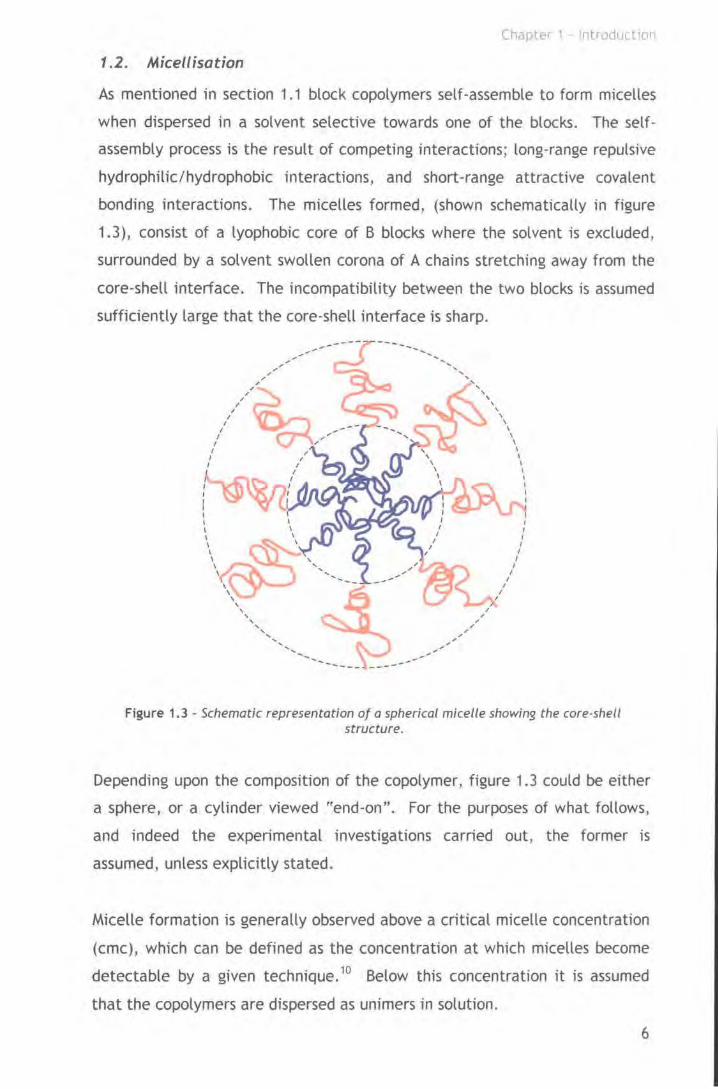
1 .2. Micellisat;on
As mentioned in section 1.1 block copolymers self-assemble to form micelles
when dispersed in a solvent selective towards one of the blocks. The self
assembly process is the result of competing interactions; long-range repulsive
hydrophilic/hydrophobic interactions, and short-range attractive covalent
bonding interactions. The micelles formed, (shown schematically in figure
1.3), consist of a lyophobic core of B blocks where the solvent is excluded,
surrounded by a solvent swollen corona of A chains stretching away from the
core-shell interface. The incompatibility between the two blocks is assumed
sufficiently large that the core-shell interface is sharp.
--- ------ .-. ---
Figure 1.3 - Schematic representation of a spherical micelle showing the core-shell structure.
Depending upon the composition of the copolymer, figure 1.3 could be either
a sphere, or a cylinder viewed "end-on". For the purposes of what follows,
and indeed the experimental investigations carried out, the former is
assumed, unless explicitly stated.
Micelle formation is generally observed above a critical micelle concentration
(cmc), which can be defined as the concentration at which micelles become
detectable by a given technique. 10 Below this concentration it is assumed
that the copolymers are dispersed as unimers in solution.
6
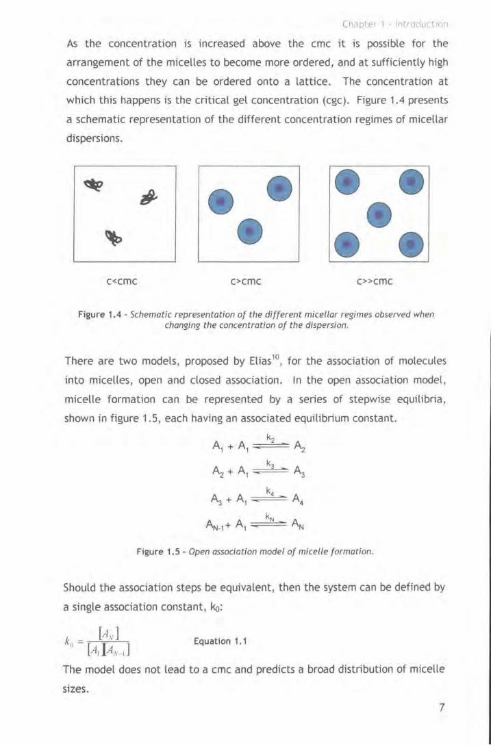
As the concentration is increased above the erne it is possible for the
arrangement of the micelles to become more ordered, and at sufficiently high
concentrations they can be ordered onto a lattice. The concentration at
which this happens is the critical gel concentration (cgc). Figure 1.4 presents
a schematic representation of the different concentration regimes of micellar
dispersions.
c<cmc c>cmc c>>cmc
Figure 1.4- Schematic representation of the different micellar regimes observed when changing the concentration of the dispersion.
There are two models, proposed by Elias10, for the association of molecules
into micelles, open and closed association. In the open association model,
micelle formation can be represented by a series of stepwise equilibria,
shown in figure 1.5, each having an associated equilibrium constant.
A1 + A1 ~
Az
Az + A1 ~
A3
A3 + A1 k4
A4
~-1 + A1 kN
AN
Figure 1. 5 - Open association model of micelle formation.
Should the association steps be equivalent, then the system can be defined by
a single association constant, ko:
k = [Av ] () [AI IA.v-1 ]
Equation 1. 1
The model does not lead to a erne and predicts a broad distribution of micelle
sizes.
7
Chapter 1 - Introduction
In the closed association model, micelle formation is represented by an
equilibrium between dispersed molecules and micelles having association
number, p, as shown in figure 1.6.
pA1 AP
Figure 1.6- Closed association model of micelle formation
The association constant, kc is given by equation 1.2.
Equation 1.2
The model does lead to a erne and predicts a narrow micelle size distribution.
The closed association model is the most applicable to block copolymer
systems, since a erne is almost invariably observed and the micelles formed
exhibit narrow size distributions.
The experimental determination of the erne is discussed in section 3.2.1.1.
1.2.1. Theoretical description of micellisation
Many models have been postulated to describe the micelles formed by block
copolymers in dilute dispersions. These can be divided into two classes:
i.) Scaling approaches, which provide simple relationships pertaining to how
micelle dimensions such as the core radius or shell thickness depend on
the number of segments of the different blocks.
ii.) Mean field models, where a block profile is usually assumed, and the
association number, erne, and phase diagram can be calculated from an
expression for the free energy.
1.2. 1.1. Scaling theories
de Gennes11 made a major advance in this area in 1978, with the scaling
relationship he proposed, essentially an extension of Alexander-de Gennes12'
13
theory for polymer brushes. In his model of a micelle he assumed that the
micelle consisted of p chains, which in the core were uniformly stretched,
giving a core radius R8• He also assumed uniform densities for the both the
core and the corona. The model was reported for the limit of short A chains, 8

Chaote1 1 lnttoductton
i.e. N6»NA, resulting in a thin corona, with the core radius expected to scale
as:
Equation 1. 3
where a is the segment length, Ne is the core chain degree of polymerisation ,
y is the interfacial tension and T is temperature
and the association number as:
'}f12 P - N - Equation 1.4 n T
Daoud and Cotton 14 formulated a model to describe star-like polymers in a
good solvent based on the principle of polymer "blobs" from Alexander-de
Gennes theory, with the chain-ends confined to a spherical surface, as in
figure 1. 7.
r
Figure 1. 7- Representation of the blob analogy utilised by Oaoud and Cotton
Unlike the de Gennes model where the polymer concentration was assumed to
be uniform across the corona, Daoud and Cotton postulated that it was
dependent upon the distance, r, from the centre of the star. This was
accomplished by increasing blob size with distance from the centre of the
star, with the result being greater swelling on the outside of the molecule.
The model can be applied to micelles by replacement of the number of arms,
f, with the association number, p. 9

Chapter 1 - Introduction
Three regions with distinct concentration profiles were identified:
i.) An inner melt-like core
ii.) An intermediate concentration region
iii.) A swollen outer region
The authors found that the radius of a star polymer in a good solvent in the
long A chain limit, scaled as:
R- N~15 fl 15 a Equation 1.5
Zhulina and Birshtein 15 applied scaling arguments to micelles, both spherical
and cylindrical, formed by diblock copolymers in selective solvents. They
identified four regimes, depending upon the composition of the copolymer,
which are shown in figure 1.8.
1 . 2
3
Figure 1.8 - Micellar regimes identified by Zhulina and Birshtein
Scaling relationships were proposed for the core radius, the shell thickness,
the association number and the interfacial area per chain for each of the four
regimes, and these are detailed in table 1.2.
10

Chapter 1 · Introduction
Regime Copolymer
Rs RA p a composition
1 N < Nv '6 A 8
N1 3 8
N'' ~
N 8 Nl.l
li
2 Nv 6 < N < N(l+2v) 6v R 1 B
N Nt•·-116•· A fi
3 N(]+l.v) (H• < 1\j Nll+2v) 5•• R I .I < B
N N-2v n+2•) 8 A
NJ' <-'-·+n A
'!Vz N-{1" 11•2••) J R A
N2•· u.1.·1 A
4 N < N<l+2vt s,. A B
NJ s B
N'' N2<1-•·l s ,., 8 N~ 5 N2 5
B
Table 1. 2 - Scaling relationships associated with each of the regimes identified by lhulina and Birshtein, along with the copolymer compositions giving rise to each.
Using the Daoud and Cotton model as a starting point, Halperin 16 produced a
scaling description of the micelles formed by AB diblock copolymers in a
highly selective solvent. The constraints of the model were that the micelles
had a small core and an extended corona (i.e. NA »N6 ), and that the micelles
were assumed to be spherical and monodisperse, each consisting of f
monomers. The concentration of the corona was not assumed to be constant,
as in the work be de Gennes, but was allowed to "fall off" as in star polymers.
i.e.
1.0 a)
1.0 b)
l 0 0
r r R
Figure 1. 9 -Plots of monomer volume fraction vs. distance from micelle centre (r). a) large core limit (N8» NA), b) small core limit (Na«NA).
Scaling relationships were produced for the radius of the core, and the overall
micelle radius, and were:
Equation 1.6
and
11

Chapter 1 - Introduction
Equation 1. 7
The scaling laws are only valid for high values of p, and therefore can only be
used to describe micelle structure beyond the erne, and not to determine the
erne itself.
All of the models discussed so far predict that the association number and
core radius are independent of the length of the chains forming the corona.
In contrast to this observation Zhang and co-workers17 produced a scaling
relationship for the core radius from the experimental data from
poly(styrene)-poly(acrylic acid) micelles in water. They found· that the core
radii determined from transmission electron microscopy (TEM) scaled as:
R ~ No.4 N-O.!s B B A Equation 1.8
The relationship was found not to be universal when applied to other
experimental data. The authors concluded that the length of the soluble
block influenced the core radius and proposed the more general relationship:
Equation 1. 9
with a and y being dependent upon the system in. question. The observation
that the length of the soluble block exerts influence on the core radius is one
that was also made by Whitmore and Noolandi, 18 and indeed Zhang et al. use
this as support for their observation.
1.2.1.2. Self-consistent field theories
Noolandi and Hong 19 proposed a model for AB diblock micelles based on a
spherical shape, and the fact that the insoluble B block forms a uniform core
and the A block forms a uniform corona. By applying a mean field theory, and
using an approximation for the surface tension, along with known copolymer
composition, molecular weight, and concentration in solution, the equilibrium
size of micelles was obtained. The theory was compared to results obtained
previously by Plestil and Baldrian20 for PS-PB micelles in heptane, and was
found to be in good agreement with the SAXS data. Agreement was also
noted with the results of de Gennes, with respect to the scaling of micelle
size, association number and radii with the degree of polymerisation.
12

Chapter 1 - Introduction
Leibler et a/. 21 proposed a mean field theory model for micelles formed by a
diblock copolymer in a homopolymer solvent. Their model allowed the
calculation of both the micelle size and the association number. The model
assumed a symmetric copolymer, i.e. NA=Ns, and that the homopolymer
chains were much shorter than those of the copolymer. Spherical morphology
was considered with a core consisting of only B blocks, and a corona
containing a fraction, 11, of A blocks and of homopolymer (1-11)· For the case
of small incompatibility between the two blocks it was found that:
p- No.6
and
Equation 1. 1 0
RB - N°. 53 Equation 1. 11
whilst for strong incompatibility
p-N
and
Equation 1. 12
Equation 1. 13
with the latter case showing good agreement with the relationships proposed
by de Gennes. 11
In an extension of the earlier work of Noolandi and Hong19, Whitmore and
Noolandi18 proposed scaling relationships for diblock copolymer micelles
dispersed in a homopolymer They found that the core radius exhibited a
slight dependence upon the length of the soluble block, with it scaling as:
RB - N t N ~ 0. 67 ~/]50.76, -0. 1 ~p50 Equation 1. 14
The corona thickness was found to scale primarily with the length of the
soluble A block, i.e.
RA - N; 0. 5~w50. 86 Equation 1. 15
The model was compared to the SANS results of Selb et al.22 They measured
the core radius of poly(styrene )-poly(butadiene) copolymers in a
poly(butadiene) homopolymer of different molecular weights. Good
agreement between theory and experiment was observed, with the exponents
of the core radius differing slightly.
13

Chapter 1 - Introduction
Nagarajan and Ganesh23 proposed a theory for the formation of block
copolymer micelles in a selective solvent. The micelles were assumed to have
a core consisting solely of the insoluble B blocks with the corona composed of
A chains and solvent. In common with the work of Whitmore and Noolandi18
the authors found that the solvent compatible block exerts an influence on
the micelle properties, especially in a good solvent. Scaling relationships
were obtained for block copolymers in a good solvent, poly(propylene oxide)
poly(ethylene oxide) in water, and in a near theta solvent, poly(butadiene)
poly(styrene) in n-heptane, and were respectively:
R . N°.1 7 N°·13 E t' 1 16 N-0·9NI.J 9 E t' 1 17. R N°.14N°·06 E t' 1 18 B - A B qua ton • p - A B qua ton • A - A B qua ton •
R N °.08N°.10 E t' 1 19 N-024NI. 10 E t' 1 20R N°·68 N°.01 E t' 1 21 B - A B qua ton . • p - A B qua ton • A - A B qua ton •
Combining these results, and those from two model systems, generic scaling
relationships were proposed:
JN2(YBsa2J+N312 +N N" 2(RBJ
113
B kT B BA R Equation 1.22
Equation 1.23
, N6!1 N-8111 ]
1/5
A-AS A B Equation 1.24
Where y65 is the interfacial tension between the B block and the solvent, and
XAs is the Flory-Huggins interaction parameter between the A block and the
solvent.
There are many other theories relating to block copolymer micelles, and the
interested reader is referred to Hamley,4 or Linse24 for further details.
1.3. Polymer Brushes
The size of an isolated polymer coil in solution is determined by the
thermodynamic quality of the solvent. In a thermodynamically good solvent
where the interactions between the chain segments and the solvent m.olecules
14
Chapter 1 lntrndufllon
are attractive, the coil will expand to maximise favourable contacts with the
solvent. In a thermodynamically poor solvent where the interactions between
the components are repulsive the coil collapses in on itself to minimise
unfavourable interactions with the solvent.
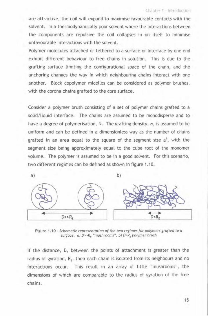
Polymer molecules attached or tethered to a surface or interface by one end
exhibit different behaviour to free chains in solution. This is due to the
grafting surface limiting the configurational space of the chain, and the
anchoring changes the way in which neighbouring chains interact with one
another. Block copolymer micelles can be considered as polymer brushes,
with the corona chains grafted to the core surface.
Consider a polymer brush consisting of a set of polymer chains grafted to a
solid/liquid interface. The chains are assumed to be monodisperse and to
have a degree of polymerisation, N. The grafting density, cr, is assumed to be
uniform and can be defined in a dimensionless way as the number of chains
grafted in an area equal to the square of the segment size a2, with the
segment size being approximately equal to the cube root of the monomer
volume. The polymer is assumed to be in a good solvent. For this scenario,
two different regimes can be defined as shown in figure 1.1 0.
a) b)
D>>R
Figure 1.10 - Schematic representation of the two regimes for polymers grafted to a surface. a) D>>R3 "mushrooms", b) D<RJ polymer brush
If the distance, D, between the points of attachment is greater than the
radius of gyration, Rg, then each chain is isolated from its neighbours and no
interactions occur. This result in an array of llttle "mushrooms", the
dimensions of which are comparable to the radius of gyration of the free
chains.
15
Chaptet 1 - lntrnduct1on
If D<Rg then the chains interact with one another. In this instance excluded
volume interactions between neighbouring chains causes them to stretch
normal to the grafting surface minimising unfavourable contact with one
another and maximising favourable contact with the solvent molecules. The
result is an array of interacting chains known as a brush.
The brush height, h, can be defined as the distance from the grafting surface
at which the polymer volume fraction equals zero, i.e. just solvent. In a good
solvent h is usually several times greater than the unperturbed radius of
gyration of the polymer chains. As the quallty of the solvent decreases the
brush layer collapses as the polymer segments attempt to minimise
unfavourable interactions with the solvent molecules.
The variation of the polymer volume fraction with distance from the grafting
surface has been a subject of numerous theoretical models. 25
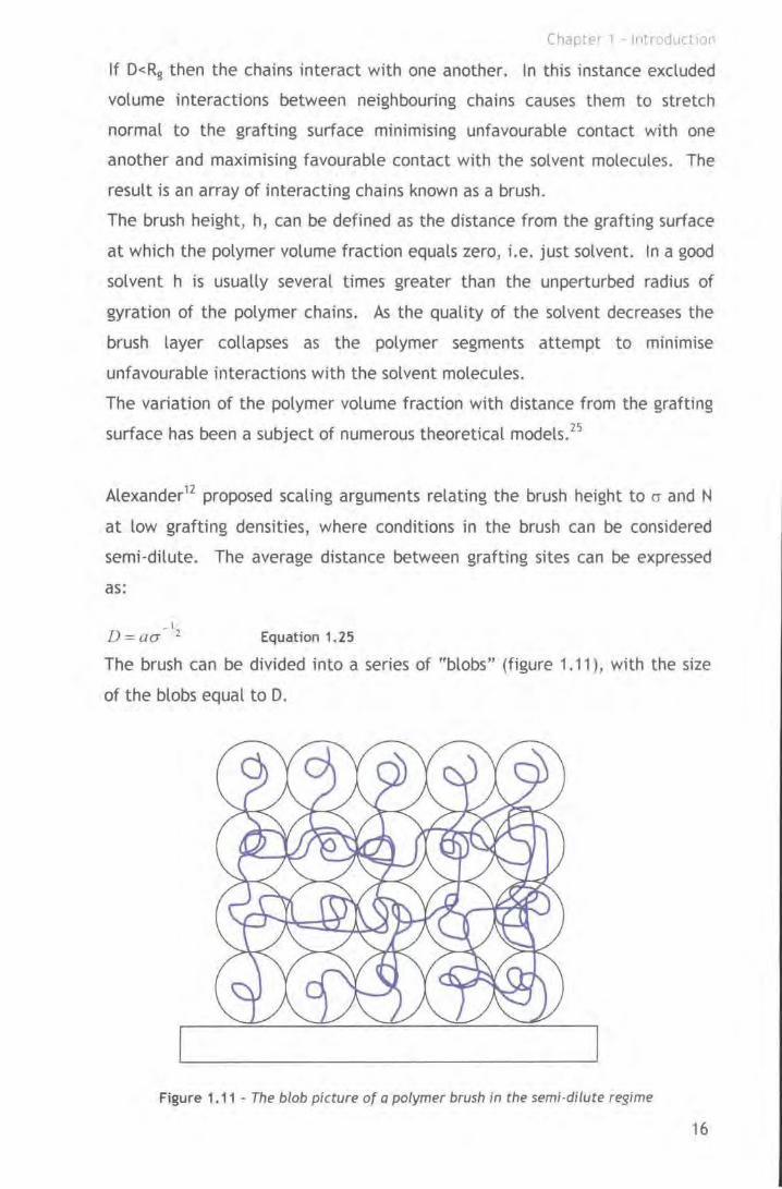
Alexander12 proposed scaling arguments relating the brush height to cr and N
at low grafting densities, where conditions in the brush can be considered
semi-dilute. The average distance between grafting sites can be expressed
as:
- I D = aa 2 Equation 1.25
The brush can be divided into a series of "blobs" (figure 1.11 ), with the size
of the blobs equal to D.
Figure 1.11 - The blob picture of a polymer brush in the semi-dilute regime
16
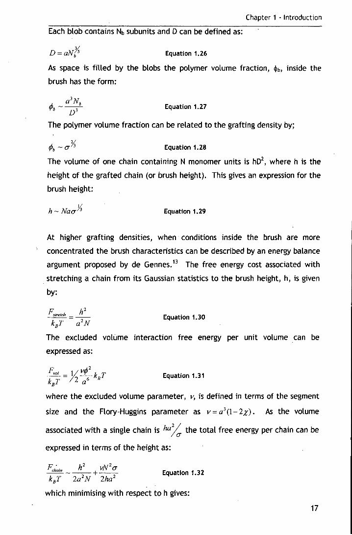
Chapter 1 - Introduction
Each blob contains Nb subunits and D can be defined as:
D=aNts Equation 1.26
As space is filled by the blobs the polymer volume fraction, <l>b, inside the
brush has the form:
Equation 1.27
The polymer volume fraction can be related to the grafting density by;
Equation 1.28
The volume of one chain containing N monomer units is hD2, where h is the
height of the grafted chain (or brush height). This gives an expression for the
brush height:
h- Naay; Equation 1.29
At higher grafting densities, when conditions inside the brush are more
concentrated the brush characteristics can be described by an energy balance
argument proposed by de Gennes. 13 The free energy cost associated with
. stretching a chain from its Gaussian statistics to the brush height, h, is given
by:
F h2 stretch --=-- Equation 1.30 k8 T a 2N
The excluded volume interaction free energy per unit volume . can be
expressed as:
Equation 1.31
where the excluded volume parameter, v, is defined in terms of the segment
size and the Flory-Huggins parameter as v = a3 (1- 2 x) . As the volume
associated with a single chain is ha% the total free energy per chain can be
expressed in terms of the height as:
Fch~in h2
vN2a -----+--
kBT 2a 2 N 2ha2 Equation 1.32
which minimising with respect to h gives:
17

Chapter 1 - Introduction
h- N(va)?; Equation 1.33
lt is evident from equations 1.29 and 1.33 that both the Alexander and the de
Gennes theories predict a linear relationship between brush height and degree
of polymerisation, and a cube-root dependence on the grafting density. Only
the latter incorporates the effect of solvent quality, with the brush height
expected to increase with the quality of the solvent.
Both models proposed by Alexander and de Gennes assume that all chains
within the brush behave the same with the free chain ends all located at the
tip of the brush. The polymer volume fraction profile corresponding to both
models is constant throughout the brush, falling abruptly to zero at the edge
of the brush, i.e. a step-function.
Milner et al. 26 used a self-consistent field model to determine the
concentration profile of polymer brushes. The solution of the SCF equations
indicated a parabolic decay could be used to represent the polymer volume
fraction within the brush, in contrast to the step function of Alexander-de
Gennes theory12•
13• In their model, the brush height, his given by:
h=(~~t N(ov)K Equation 1.34
Equation 1.34 shows that the brush height predicted by SCFT has the same
cube root dependence on N and cr as the scaling relationships of Alexander12
and de Gennes. 13 Unlike the scaling arguments that assume all the chains
behave alike, with their free ends located at the tip of brush, the SCF
calculations reveal that the free chain ends are distributed throughout the
entire brush. These differences mean that scaling theory predicts a step
function for the volume fraction profile whilst SCFT predicts a parabolic
profile, as shown in figure 1.12.
18

Chapte• 1 • lntroducuor
z z = h
Figure 1.12 • representation of step function predicted by Alexander-de Gennes theory, and the parabolic volume fraction - due to the SCFT of Milner et a/. 16
1.4. Micellar behaviour of poly(butadiene)-poly(ethylene oxide)
Investigations into the micellar behaviour of poly(butadiene)·poly(ethylene
oxide) (PB-PEO) have only begun to appear in the literature within the last
five or so years. Many of the investigations have been carried out in the group
of Frank Bates, these are reviewed first, followed by investigations made by
others.
1.4. 1. Investigations of the Bates group
Won , Davis and Bates27 investigated the solution behaviour of a PB-PEO
diblock copolymer of molecular weight 4900g mol"1 containing 50wt% PEO in
water at concentrations of up to 17%, and temperature between 298 and
348K. They observed that under all conditions cylindrical micelles consisting
of a PB core surrounded by a PEO corona were formed . Small angle X-ray and
neutron scattering (SAXS and SANS) were used to probe the ordering of the
micelles over the concentration and temperature range stated, and a phase
diagram was constructed (fig 1.13)
19

Chaptet 1 - lntrodUCtlO•t
34)
lll ?l , ~
lm t"' 310
Hexagonal Isotropic Nematic
DJ
0 2 4 6 8 10 12 14 16
Cqrlyrra-Ol 03 traticnlv.t%
Figure 1. 13 - Phase diagram as a function of temperature and concentration for micelles of PB-PEO investigated by Won, Da0s and Bates. Replicated from reference 27.
The phase diagram shows that below 5% the micelles were present as an
isotropic dispersion. As the concentration was increased, so did the order of
the system and a one-dimensional ordered Nematic phase was observed
between 5 and 10%. At concentrations greater than 10% the cylinders were
ordered on a regular hexagonal lattice. Cryo-Transmission electron
microscopy (cryo-TEM) yielded some interesting micrographs, with the long
worm-like micelles clearly visible.
The authors cross-linked the PB core of the micelles using a redox
combination of potassium persulphate, sodium metabisulphite, and iron(ll)
sulphate heptahydrate, which allowed coupling of the 1 ,l double bonds of the
PB backbone. SANS was used to investigate the differences between the
micelles before and after cross-linking, with a reduction in the core radius of
13% observed. lt was also noted that the cross-linking was confined to the
core of the micelles by comparing solutions cross-linked at 5% then diluted
ten-fold, to those cross-linked at 0.5%, with the scattering being
indistinguishable between the two. This fact suggested that both solutions
have the same inter and intra micellar structure.
Zheng et al.28 used cryo-TEM to image vitrified films of PB-PEO dispersions.
Several copolymers were used, having molecular weights in the range 4900-
20
Chapter 1 - Introduction
131 OOg mol"1 and PEO contents between 51 and 70%. The authors noted that
those copolymers with the lower PEO content formed cylindrical micelles,
whilst those with the higher PEO content formed spheres when dispersed in
water. The dimensions of the two morphologies were similar with the
cylinders having a core radius of 160A and total radius 490A, whilst those of
the spheres were 150A and 480A respectively. Comparisons of the ratio of
Rcore: Rtotat were made with the star model of Halperin 16 and the mean field
model of liebler et al. 21 with the former providing the better agreement.
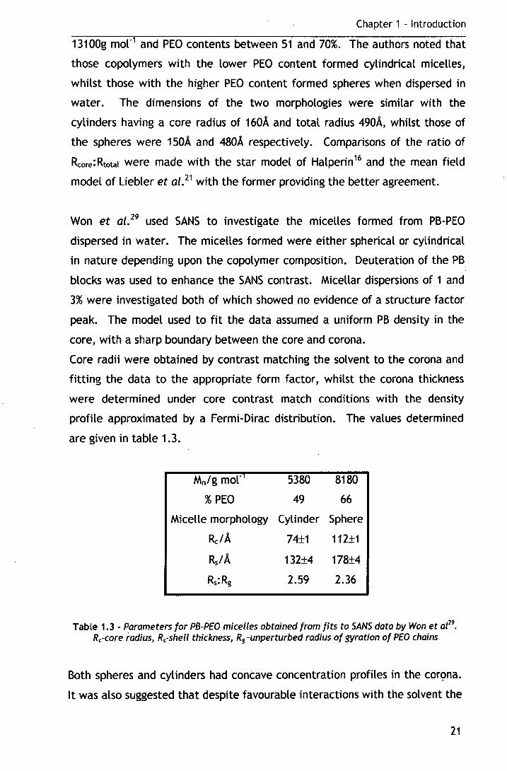
Won et al. 29 used SANS to investigate the micelles formed from PB-PEO
dispersed in water. The micelles formed were either spherical or cylindrical
in nature depending upon the copolymer composition. Deuteration of the PB
blocks was used to enhance the SANS contrast. Micellar dispersions of 1 and
3% were investigated both of which showed no evidence of a structure factor
peak. The model used to fit the data assumed a uniform PB density in the
core, with a sharp boundary between the core and corona.
Core radii were obtained by contrast matching the solvent to the corona and
fitting the data to the appropriate form factor, whilst the corona thickness
were determined under core contrast match conditions with the density
profile approximated by a Fermi-Dirac distribution. The values determined
are given in table 1.3.
Mn/g mol" 1 5380 8180
% PEO 49 66
Micelle morphology Cylinder Sphere
Re/A 74±1 112±1
RsiA. 132±4 178±4
Rs:Rg 2.59 2.36
Table 1.3 - Parameters for PB-PEO micelles obtained from fits to SANS data by Won et al29•
Re-core radius, R5-shell thickness, Rg-unperturbed radius of gyration of PEO chains
Both spheres and cylinders had concave concentration profiles in the cor~ma.
lt was also suggested that despite favourable interactions with the solvent the
21

Chapter 1 - Introduction
ethylene oxide segments were accumulated next to the core, possibly
shielding it from unfavourable interactions with the solvent.
Won et al. 30 investigated the differences between core· cross-linked and
unreacted worm-like micelles in terms of their rheological properties and
depletion effects upon the addition of PEO. The cross-linking was
accomplished using the same redox combination detailed in their earlier
paper, with a polymer of 4900g mol"1 and 50% PEO being used.
The authors observed that the cross-linked micelles had a storage modulus
that was more than two orders of magnitude larger than their unreacted
counterparts, which was attributed to an elastically interacting physical
network of the cross-linked micelles. Also when subjected to shear the cross
linked micelles retained their orientation isotropy in contrast to the
unreacted micelles, which aligned in the flow direction.
Using a series of PB-PEO block copolymers ranging in molecular weight from
3600 to 13100g mol"1 and PEO compositions from 28 to 66%, as well as some
poly(ethyl ethylene)-poly(ethylene oxide) di and tri-block copolymers, Won et
al. 31 utilised cryo-TEM to determine the boundaries for shape transitions
between different morphologies. This led to the construction of a morphology
diagram as function of PEO volume fraction in the polymer, and length of the
hydrophobic block, as shown in figure 1.14. The vertical lines on the
morphology diagram serve merely as an indication of the boundaries and are
not absolute.
22

Chapter 1 - Introduction
o PB-PEO 4 PEE-PEO 0 PEO-PEE-PEO
0 100
B C C+S s 80
0 0
40
20
a~~~~~~~~~~~~~~~
0.2 0.3 0.4 0.5 0.6 0.7
Figure 1.14- Morpholc;Jgy diagram as a function of PEO composition, fE0 , and PB degree of polymerisation, Ncore, from Won et al. 31 8-Bilayered vesicles, C-cylinders, S-spheres
In addition to the basic geometries of membrane-like bilayer, cylinder and
sphere, more exotic compound structures were observed in the ranges near to
the bilayer-cylinder and cylinder-sphere boundaries. These structures were
observed in both freshly prepared and long-term stored solutions indicating
their long lifetime. Their presence was attributed to the metastability of
amphiphilic polymeric materials.
Packing properties such as the interfacial area per chain and degree of
hydrophobic stretching were determined, and it was noted that for a given
morphology the interfacial area per chain was inversely proportional to the
hydrophobic stretching.
Jain and Bates32 investigated the solution properties of two series of PB-PEO
diblock copolymers, each having constant PB molecular weights, but varying
PEO content. One of PB molecular weight 2500g mor1 and 0.3;s:;wpEO;s:;0.64, and
the other of 9200 g mor1 and 0.24;s:;wpE0;s:;0.62. 1% dispersions were examined
using cryo-TEM, and the authors were able to construct a morphology diagram
(figure 1.15) relating the morphology observed to the degree of
polymerisation of PB and the PEO content of the copolymer.
23

Chapter 1 - Introduction
200 ~ \
160
120
• \. \~\ . ~~c\ \ c
·. Y·. ·. y
\ \_\
•
z!-80
B B+C s 40
0 0.2 0.3 0.4 0.5 0.6 0.7
w PEO
Figure 1. 15 - Morphology diagram as a function of PEO composition, wPE0 , and PB degree of polymerisation, Np8 , from Jain and Bates. 32 Abbreviations as in figure 1.14, and N-Network,
Cy-cylinder with Y-junctions
In common with the work of Won et al. 31 they ob~erved the "classical"
sequence of dispersed structures, i.e. bilayered vesicles, cylinders and
spheres with increasing PEO content. The large increase in copolymer
molecular weight caused the core dimensions to increase three fold, and shift
the morphology boundaries to lower PEO content, as shown in figure 1.15.
They also observed the formation of Y -junctions in cylindrical micelles at
compositions between the B and C regimes. Even at WpE0=0.42 where
cylinders would be expected occasional branches were observed. At
WpEO=O. 39 an extended three-dimensional network morphology dominated by
Y -junctions was formed; behaviour that was not observed in the lower
molecular weight copolymers. Fragmentation of the network by stirring or
sonication produced individual micelles of complex morphology, exhibiting a
high degree of symmetry. The authors attributed this to the redistribution of
diblock copolymer molecules within the particles after fragmentation in order
to balance the internal energy.
Won, Davis and Bates33 used a combination of fully hydrogenous and dPB-hPEO
to investigate the molecular exchange in spherical and cylindrical micelles.
They examined 1% dispersions that were prepared using two different
methods:
24
Chapter 1 - Introduction
i.) Pre-mixing, where both isotopic variants were dissolved in chloroform,
dried, annealed, then dispersed in 020.
ii.) Post-mixing, where 1% dispersions of both isotopic variants were mixed
directly.
SANS experiments on dispersions produced by the two methods revealed
differences in the scattering curves. The eight-day-old post-mixed sample·
could be accurately reproduced by scattering from an unmixed sample (the
mean of the scattering from the two isotopic variants), suggesting that no
exchange had taken place. The authors concluded that intermicellar
equilibration time may be of the order of years, and that the residence time
of a copolymer molecule within a micelle may be immeasurably large.
1.4.2. Investigations by other researchers
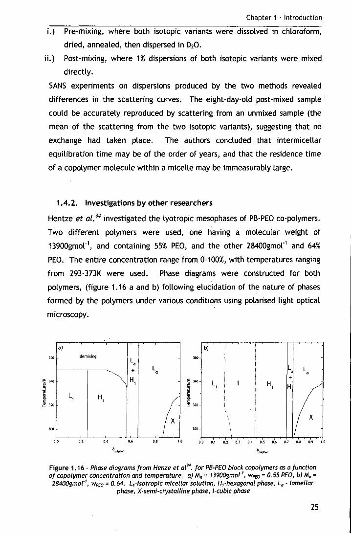
Hentze et al. 34 investigated the lyotropic mesophases of PB-PEO co-polymers.
Two different polymers were used, one having a molecular weight of
13900gmor1, and containing 55% PEO, and the other 28400gmol"1 and 64%
PEO. The entire concentration range from 0-100%, with temperatures ranging
from 293-373K were used. Phase diagrams were constructed for both
polymers, (figure 1.16 a and b) following elucidation of the nature of phases
formed by the polymers under various conditions using polarised light optical
microscopy.
a) b)
360 demixing L 360
a L + a
L L a
~ H1 ~340 ~340 +
L1 H1 i ~ H "' l ~ 320
L1 H1 ~ 320
300 300
0.0 0.2 0.4 0.6 0.8 1.0 0.0 0.1 0.2 0.3 0.4 0.5 0.6 0.7 0.8 0.9 1.0
Figure 1.16 - Phase diagrams from Henze et al34• for PB-PEO block copolymers as a function
of copolymer concentration and temperature. a) Mn = 13900gmot1, wPEO = 0.55 PEO, b) Mn =
28400gmot 1, Wp£o = 0.64. L1-isotropic micellar solution, H1-hexagonal phase, La- lamellar
phase, X-semi-crystalline phase, /-cubic phase
25
Chapter 1 - Introduction
Cross-linking of the ordered phases, using y-rays, resulted in the formation of
solid, mechanically stable, "elastic" hydrogels that swelled on the addition of
water but did not dissolve. The morphology of the mesophases was retained
upon cross-linking, and SAXS measurements revealed a decrease of 5-10% in
the d-spacings.
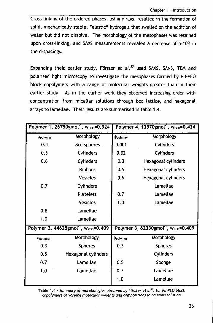
Expanding their. earlier study, Forster et al. 35 used SAXS, SANS, TEM and
polarised light microscopy to investigate the mesophases formed by PB-PEO
block copolymers with a range of molecular weights greater than in their
earlier study. As in the earlier work they observed increasing order with
concentration from micellar solutions through bee lattice, and hexagonal
arrays to lamellae. Their results are summarised in table 1.4.
Polymer 1, 26750gmor•, WPEo=0.524 Polymer 4, 13570gmor•, WPEo=0.434
~polymer Morphology ~polymer Morphology
0.4 Bee spheres . 0.001 Cylinders
0.5 Cylinders 0.02 Cylinders
0.6 Cylinders 0.3 Hexagonal cylinders
Ribbons 0.5 Hexagonal cylinders
Vesicles 0.6 Hexagonal cylinders
0.7 Cylinders Lamellae
Platelets 0.7 Lamellae
Vesicles 1.0 Lamellae
0.8 Lamellae
1.0 Lamellae
Polymer 2, 44625gmor1, WpEQ=0.409 Polymer 3, 82330gmor\ WpEo=0.409
~polymer Morphology ~polymer Morphology
0.3 Spheres 0.3 Spheres
0.5 Hexagonal cylinders Cylinders
0.7 Lamellae 0.5 Sponge
1.0 Lamellae 0.7 Lamellae
1.0 Lamellae
Table 1.4 - Summary of morphologies observed by Forster et al35• for PB-PEO block
copolymers of varying molecular weights and compositions in aqueous solution
26

Chapter 1 - Introduction
They noted that increasing the molecular weight of the copolymer reduced
the order in the system, especially in the bee lattice and hexagonal regimes.
In common with the work of the Bates group, the formation of loops and
junctions from cylindrical morphology was observed.
Egger et al. 36 investigated a mixed system of PB-PEO and
Dodecyltrimethylammoniumbromide, DTAB, using light scattering, SAXS and
SANS. The polymer they used had a molecular weight of 4330gmol"1, a PEO
content of 54% and formed cylindrical micelles upon dispersion in water.
Adding DTAB at concentrations greater than its erne resulted in a
transformation from cylindrical to spherical morphology being observed. The
authors proposed that this was due to the formation of mixed micelles, the
driving force for which was the dilution of charges by embedding the cationic
surfactant head group in the matrix of neutral ethylene oxide segments.
Maskos and Harris37 investigated the micellar structures of a PB-PEO diblock
copolymer of molecular weight 3350gmol"1 containing 40% PEO. A dispersion
of ea 0.1% was cross-linked using y-rays, and the structures produced, the
most common of which were bilayered vesicles, imaged using TEM. The
authors noted that the vesicles were s~able enough to be transferred to THF,
a good solvent for both blocks, whilst retaining the same shape. Small
numbers of other structures were observed such as cylinders, strings of
vesicles and vesicle sheets. The authors suggested that the strings were
formed by fusion of the outer layers of the vesicles.
1.5. Micellar behaviour of poly(butylene oxide)-poly(ethylene oxide)
Over the last decade or so, Booth and eo-workers have investigated the
micellisation of poly(butylene oxide)-poly(ethylene oxide) (PBO-PEO) in
aqueous solution. For brevity a brief summary of the important conclusions is
presented here, and the interested reader is referred to recent reviews
summarising their efforts and the references contained therein for more
detail. 38'
39
27
Chapter 1 lnt r oducr H'lfl
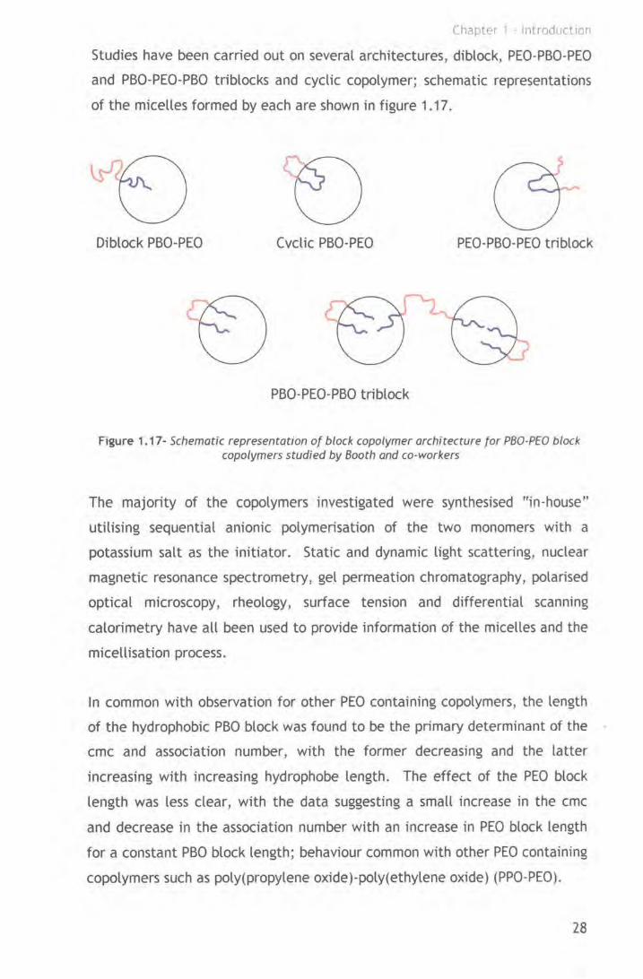
Studies have been carried out on several arch1tectures, diblock, PEO·PBO·PEO
and PBO·PEO·PBO triblocks and cyctk copolymer; schematic representations
of the micelles formed by each are shown in figure 1.17.
Diblock PBO-PEO Cvclic PBO-PEO PEO-PBO-PEO triblock
PBO-PEO-PBO triblock
Figure 1.17- Schematic representation of block. copolymer architecture for PBO-PEO block copolymers studied by Booth and eo-workers
The majority of the copolymers investigated were synthesised 11in-house"
utilising sequential anionic polymerisation of the two monomers with a
potassium salt as the initiator. Static and dynamic light scattering, nuclear
magnetic resonance spectrometry, gel permeation chromatography, polarised
optical microscopy, rheology, surface tension and differential scanning
calorimetry have all been used to provide information of the micelles and the
micellisation process.
In common with observation for other PEO containing copolymers, the length
of the hydrophobic PBO block was found to be the primary determinant of the
erne and association number, with the former decreasing and the latter
increasing with increasing hydrophobe length. The effect of the PEO block
length was less clear, with the data suggesting a small increase in the erne
and decrease in the association number with an increase in PEO block length
for a constant PBO block length; behaviour common with other PEO containing
copolymers such as poly(propylene oxide)-poly(ethylene oxide) (PPO-PEO).
28
Chapter 1 - Introduction
Increasing the temperature resulted in a decrease in the erne, an observation
that was common to all of the architectures studied, whilst the association
number increased with a temperature as the quality of the· solvent for PEO
decreased. The hydrodynamic radii exhibited little temperature dependence,
an effect observed for PPO-PEO block copolymers and that was attributed to a
balance between an increase in association number, accompanied by a
decrease in the swelling of the PEO block corona as the solvent quality
decreases.
The enthalpy of micellisation was determined for a number of solutions by
plotting log (c) vs. 1/cmt, yielding values in the range 24s~micH0s125 kJ mol"1,
smaller than those determined for PPO-PEO copolymers (115s~micH0s331 kJ
mor1 ). The standard Gibbs energies were comparable to those of PPO-PEO
block copolymers, with values of -10s~micG 0s-30 kJ mor1• The results
indicated the entropy driven nature of the micellisation of PBO-PEO in
aqueous solution, which is consistent with the hydrophobicity of the PBO
block.
Comparisons were made between the different architectures at constant
composition and chain length, and for a given hydrophobe length, the erne's
were found to be in the order PBO-PEO<cyclic PBO-PEO<PBO-PEO-PBOsPEO
PBO-PEO. The association number was found to follow a similar trend, but
with the two triblock architectures forming micelles having approximately
equivalent association numbers.
1.6. Micellar behaviour of poly(propylene oxide)-poly(ethylene oxide)
Much research has been devoted to the study of the commercially available
poly(propylene oxide)-poly(ethylene oxide) (PPO-PEO) block copolymers.
There are in excess of 1000 papers relating to the micellisation properties of
these copolymers. Chu and Zhou40 recently collated and summarised ~ome of
the important results from different groups relating to the micellisation
process and resulting micelle structures. The results are complicated by the
high polydispersities of the commercially manufactured triblock copolymers as
well as the large numbers of polymer available. In addition to these
29
Chapter 1 - Introduction
complications, there are also some slight discrepancies between results
obtained from different techniques or laboratories. Never the less, some
useful comparisons can be made between the data and some interesting
trends observed.
The properties of PPO-PEO copolymers in aqueous solution are strongly
temperature dependent, with the hydrophobic nature of the PPO block
increasing with temperature. Homo-PPO is water-soluble at temperatures
below ea 283-288K, as a result PPO-PEO block copolymers exist in solution as
dispersed unimers at lower temperatures.
From the data summarised by Chu and Zhou40 it is possible to make some
generalisations about the micellisation process and the resulting structures:
i.) For a given temperature, increasing the length of the PPO block results in
an exponential decrease of the erne.
ii.) The effect of the PEO block length is less pronounced than that of the
PPO block, with only small increases in the erne and cmt observed on
increasing its length.
iii.) For a constant copolymer composition the erne and cmt values decrease
with increasing copolymer molecular weight.
iv.) The chain architecture has a profound effect on the micelle formation
with PPO-PEO-PPO copolymers displaying reduced micellisation ability in
comparison to a PEO-PPO-PEO copolymer of the same composition.
v.) The micellisation process is entropically driven, with a large positive
enthalpy of micellisation commonly observed.
vi.) The association number increases with temperature, whilst the micelle
radius remains relatively constant.
vii.) Increasing the length of the PPO block results in an increase in association
number, this is also observed for decreasing length of PEO block.
1.7. Cross-linked micelles
As discussed in section 1.1 the self-assembly process leading to the formation
of micelles is the result of non-covalent interactions; consequently the
process is reversible, and the micelles are capable of reverting back to
dispersed molecules should the conditions be suitable, e.g. dilution to c<cmc.
As has been discussed in section 1.4 for PB-PEO block copolymers it is possible
30
Chapter 1 - Introduction
to render the micelles permanent structures by chemically cross-linking the
core either though redox chemistry or y irradiation. There are however other
examples reported in the literature of cross-linked micelles in both aqueous
and hydrocarbon media. Depending upon the chemical functionality of the
block copolymer forming the micelles it is possible to effect cross-linking in
the core as already seen, or in the shell. This section aims to provide an
overview of both types of cross-linking.
1. 7. 1. Core cross-linked micelles
One of the earliest reports of micelle cross-linking was that of Tuzar and eo
workers. 41 They cross-linked the poly(butadiene) cores of poly(butadiene )
poly(styrene), (PB-PS), micelles in several mixed solvent systems selective for
the PS using either UV radiation and a peroxide initiator or a high energy
electron beam. ·They reported little in terms of the micelle properties either
before or after cross-linking.
Wilson and Riess42 also used UV radiation and a photo initiator, to cross-link
micelles of the same chemical nature (i.e. PB-PS in solvents selective for PS)).
Two different solvents were used, namely DMF and DMA, depending upon the
solubility of the polymer. The cross-linking efficiencies were determined by
precipitation into methanol, followed by THF addition to solubilise any non
stabilised material, and ranged from 23-86%. QELS was used to determine the
hydrodynamic radii of the micelles both before and after the cross-linking
reaction. In all cases a small decrease in Rh was observed upon cross-linking,
which the authors attributed to reduced swelling of the core by the solvent.
Saito and lshizu43 cross linked the 2-vinyl pyridine core of poly(vinyl pyridine)
poly(styrene )-poly(vinyl pyridine) (PVP-PS-PVP) triblock copolymers in
toluene/cyclohexane mixtures using 1,4 diiodobutane. TEM and QELS were
used to study the micelles before and after cross-linking, with the latter
revealing that the hydrodynamic radii of the micelles decreased upon cross
linking in toluene, but remained unchanged when the reaction was carried out
in toluene/cyclohexane.
31
Chapter 1 - Introduction
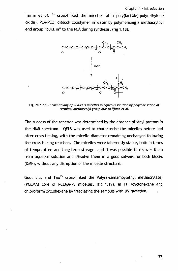
lijima et al. 44 cross-linked the micelles of a poly(lactide)-poly(ethylene
oxide), PLA-PEO, diblock copolymer in water by polymerising a methacryloyl
end group "built in" to the PLA during synthesis, (fig 1.18).
V-65
4--, C~ CH2
CHCHpHpfcHpHpLLc-tH okc-t-c~ 11 Jnl 11 }.lL o o _ I
Figure 1.18 - Cross-linking of PLA-PEO micelles in aqueous solution by polymerisation of terminal methacrolyl group due to lijima et al.
The success of the reaction was determined by the absence of vinyl protons in
the NMR spectrum. QELS was used to characterise the micelles before and
after cross-linking, with the micelle diameter remaining unchanged following
the cross-linking reaction. The micelles were inherently stable, both in terms
of temperature and long-term storage, and it was possible to recover them
from aqueous solution and dissolve them in a good solvent for both blocks
(DMF), without any disruption of the micelle structure.
Guo, Liu, and Tao45 cross-linked the Poly(2-cinnamoylethyl methacrylate)
(PCEMA) core of PCEMA-PS micelles, (fig 1.19), in THF /cyclohexane and
chloroform/cyclohexane by irradiating the samples with UV radiation.
32

Chapter 1 - Introduction
I cross-linkable double bond
Figure 1.19 - structure of PCEMA-PS block copolymer as prepared by Guo, Uu and Tao, with the site of cross-linking indicated.
The resulting particles were characterised by QELS, GPC and TEM. The
success of the reaction was demonstrated by the bimodal GPC trace, one peak
corresponding to the copolymer, and the other, of a much greater intensity,
to the cross-linked micelles; the former was attributed to unimers in
equilibrium with the micelles prior to cross-linking. QELS experiments on the
micelles before and after cross-linking revealed a slight decrease in the
hydrodynamic radius but still with a monomodal size distribution. The
decrease in size was attributed to a possible reduction in core volume upon
polymerisation. TEM revealed the micelles to be spherical in nature.
Henselwood and Liu46 cross-linked the PCEMA core of PCEMA-poly(acylic acid)
(PAA) micelles in water /DMF (80:20) mixtures by irradiation with UV light.
Characterisation of the cross-linked micelles with TEM confirmed their
spherical nature. QELS experiments were only carried out after the cross
linking reaction and so it was not possible to determine whether the micelle
· size had changed.
Rheingans et al. 47 cross-linked the poly(dimethyl siloxane) core of PDMS-PEO
micelles in water by photopolymerisation of methacrylic acid groups in the
DMS core, (fig 1.20)
33
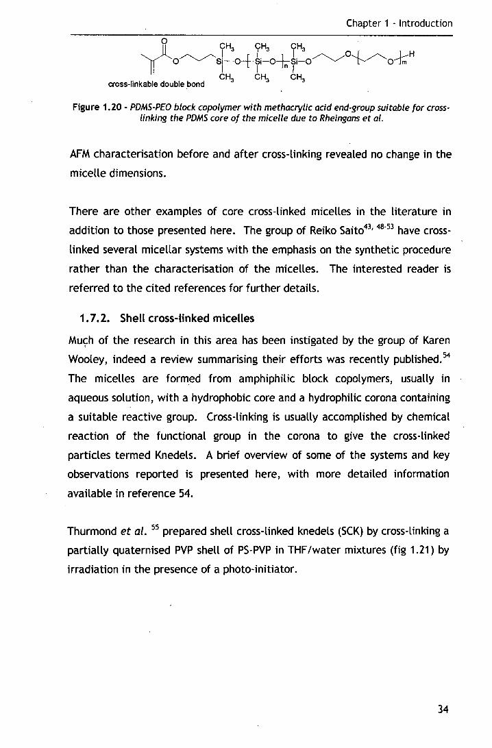
Chapter 1 - Introduction
0 .
Y CH3 CH3 CH3 I I I /"-.._ /o ... J /'-. L-H
O~Si-o+si-O_l_Si-0' '-../ ~ 'o-Jm I I Tn1 CH3 CH3 CH3 cross-linkable double bond
Figure 1.20- PDMS-PEO block copolymer with methacrylic acid end-group suitable for crosslinking the PDMS core of the micelle due to Rheingans et al.
AFM characterisation before and after cross-linking revealed no change in the
micelle dimensions.
There are other examples of core cross-linked micelles in the literature in
addition to those presented here. The group of Reiko Saito43•
48"53 have cross
linked several micellar systems with the emphasis on the synthetic procedure
rather than the characterisation of the micelles. The interested reader is
referred to the cited references for further details.
1. 7.2. Shell cross-linked micelles
Mu<;:h of the research in this area has been instigated by the group of Karen
Wooley, indeed a review summarising their efforts was recently published. 54
The micelles are formed from amphiphilic block copolymers, usually in
aqueous solution, with a hydrophobic core and a hydrophilic corona containing
a suitable reactive group. Cross-linking is usually accomplished by chemical
reaction of the functional group in the corona to give the cross-linked
particles termed Knedels. A brief overview of some of the systems and key
observations reported is presented here, with more detailed information
available in reference 54.
Thurmond et al. 55 prepared shell cross-linked knedels (SCK) by cross-linking a
partially quaternised PVP shell of PS-PVP in THF /water mixtures (fig 1.21) by
irradiation in the presence of a photo-initiator.
34

Chapter 1 - Introduction
hv
Cl
Figure 1.21 -Cross-linking reaction of the part-quaternised PVP shell of PS-PVP copolymer micelles due to Thurmond et al.
AFM was used to determine the size of the SCK's, with large variations in size
observed depending upon the relative block lengths. Typical diameters were
of the order of 10-300A for copolymers of molecular of ea. 15000 gmor1•
PS-PAA micelles in THF /water mixtures were cross-linked by amidation of the
acid group by Huang et al 56 (figure 1.22).
Figure 1.22 - cross-linking reaction of PAA corona of PS-PAA micelles by amidation reaction. due to Huang et al.
The sizes and shapes of the SCK's were studied and compared to the micelles
by AFM and TEM. lt was observed that the micelle height when adsorbed onto
35
Chapter 1 - Introduction
mica was less than that of the SCK's, which was attributed to spreading of the
micelles whilst the SCK's remained spherical in shape due to their more rigid
structure. This observation was supported by TEM, which showed the micelles ' to be ellipsoidal in shape whilst the SCK's remained spherical.
Other systems have been exploited including poly(~>-caprolactone-acrylic
acid). 57 The poly( acrylic acid) shell was cross-linked by reaction with the
amine groups of 2,2'(ethylendioxy)bis(ethylamine).
1.8. Aims and objectives
The aims and objectives of the research presented in this thesis can be
summarised as follows.
• To synthesise two molecular weight series of poly(butadiene)
poly(ethylene oxide) diblock copolymers with fully hydrogenous and
perdeuterated variants. Each copolymer should contain ea. 15wt%
poly(butadiene) which should have a majority 1,2 microstructure.
• To elucidate the structure of the micelles formed by the copolymers upon
dispersion in aj:tueous solution.
• To probe the organisation of the micelles at higher concentrations and to
determine subsequent inter-micellar interactions.
• To develop a synthetic procedure to facilitate the cross-linking of
poly(butadiene) core of the micelles without disrupting the local
structure.
• To characterise the cross-linked micelles in terms of their structure and
organisation, comparing them to the virgin micelles and rationalising any
differences.
36

Chapter 1 - Introduction
1. 9. Glossary of symbols
The symbols used in the body of the text and the equations are defined here
in the order in which they appear in the text.
1. 9. 1. Micellisation
p
Rs
a
Ns y
T
r
V
YBS
ks
micelle association number
core radius formed by insoluble B block
segment length
degree of polymerisation of insoluble block
interfacial tension
temperature
distance from micelle/star centre
number of arms in a star
degree of polymerisation of soluble block
distance between coronal chains on core surface
exclude volume parameter
interfacial tension between insoluble B block and solvent
Bolztman constant
1.9.2. Polymer Brushes
D
Rg
a
0'
fstretch
ks
T
fvol
V
X
z
separation distance between grafted chains
radius of gyration
segment length
grafting density
degree of polymerisation of brush forming layer
number of segments in a blob
polymer volume fraction inside a blob
brush height
stretching free energy
Boltzman constant
temperature
excluded volume interaction free energy
excluded volume parameter
Flory-Huggins interaction parameter
distance from grafting surface
37

Chapter 1 - Introduction
1.10. Bibliography
2
3
4
5
6
7
8
9
10
11
12
13
14
15
16
17
18
19
20
21
22
23
G. Riess, G. Hurtrez, and P. Badahur, in 'Enclycopedia of Polymer
Science and Engineering', ed. H. F. Mark and J. I. Kroschwitz, Wiley,
New York, 1985.
A. M. Urbas, et al., Adv. Mater., 2002, 14, 1850.
F. 5. Bates and G. H. Fredrickson, Annu. Rev. Phys. Chem., 1990, 41,
525.
I. W. Hamley, The Physics of Block Copolymers', Oxford University
Press, New York, 1998.
F. 5. Bates and G. H. Fredrickson, Phys. Today, 1999, 52, 32.
5. Forster and T. Plantenberg, Agnew. Chem. lnt. Ed., 2002, 41, 688.
M. Muthukumar, C. K. Ober, and E. l. Thomas, Science, 1997, 277,
1225.
M. 5zwarc, Nature, 1956, 178, 1168.
5. Forster and M. Antonietti, Adv. Mater., 1998, 10, 195.
H. G. Elias, in 'Light Scattering from Polymer Solutions', ed. M. B.
Huglin, Academic Press, London, 1972.
P. G. de Gennes, in 'Solid State Physics, Supplement', ed. l. Liebert,
Academic, New York, 1978.
5. Alexander, J. Physique, 1977, 38, 983.
P. G. de Gennes, J. Physique, 1976, 37, 1445.
M. Daoud and J. P. Cotton, J. Physique, 1982, 43, 531.
E. B. Zhulina and T. M. Birshtein, Polymer Science USSR, 1986, 27, 570.
A. Halperin, Macromolecules, 1987, 20, 2943.
l. Zhang, R. J. Barlow, and A. Eisenberg, Macromolecules, 1995, 28,
6055.
M. D. Whitmore and J. Noolandi, Macromolecules, 1985, 18, 657.
J. Noolandi i:ind K. M. Hong, Macromolecules, 1983, 16, 1443.
J. Plestil and J. Baldrian, Macromol. Chem., 1975, 176, 1009.
l. Leibler, H. Orland, and J. C. Wheeler, J. Chem. Phys., 1983, 79,
3550.
J. 5elb, et al., Polymer Bulletin, 1983, 10, 444.
R. Nagarajan and K. Ganesh, J. Chem. Phys., 1989, 90, 5843.
38
24
25
26
27
28
29
30
31
32
33
34
35
36
37
38
39
40
41
42
43
44
45
46
47
48
49
Chapter 1 - Introduction
P. linse, in 'Amphiphilic block copolymers: Self assembly and
applications', ed. P. Alexandridis and B. lindman, Elsevier, Amsterdam,
2000.
R. A. L. Jones and R. W. Richards, 'Polymers at Surfaces and Interfaces',
Cambridge University Press, Cambridge, 1999.
S. T. Milner, T. A. Witten, and M. E. Cates, Macromolecules, 1988, 21,
2610.
Y. Y. Won, H. T. Davis, and F. S. Bates, Science, 1999, 283, 960.
Y. Zheng, et al., J. Phys. Chem. 8, 1999, 103, 10331.
Y. Y. Won, et al., J. Phys. Chem. 8, 2000,104,7134.
Y. Y. Won, et al.,.). Phys. Chem. 8, 2001, 105, 8302.
Y.-Y. Won, et al., J. Phys. Chem. 8, 2002, 106, 3354.
S. Jain and F. S. Bates, Science, 2003, 300, 460.
Y. Y. Won, H. T. Davis, and F. S. Bates, Macromolecules, 2003, 36, 953.
H. P. Hentze, et al., Macromolecules, 1999, 32, 5803.
S. Forster, et al., Macromolecules, 2001, 34, 4610.
H. Egger, et al., Macromol. Symp., 2000, 162, 291.·
M. Maskos and J. R. Harris, Macromolecular Rapid Communication$,
2001' 22, 271.
C. Booth and D. Attwood, Macromol. Rapid Commun., 2000, 21, 501.
C. Booth, G. E. Yu, and V. M. Nace, in 'Amphiphilic block copolymers:
Self assembly and applications', ed. P. Alexandridis and B. lindman,
Elsevier, Amsterdam, 2000.
B. Chu and Z. Zhou, in 'Nonionic surfactants: Polyoxyalkylene block
copolymers', ed. V. M. Nace, Marcel Dekker, New York, 1996.
Z. Tuzar, et al., Macromol. Chem. Phys., 1982, 183, 399.
D. J. Wilson and G. Reiss, European Polymer Journal, 1988, 24, 617.
R. Saito and K. lshizu, Polymer, 1997, 38, 225.
M. lijima, et al., Macromolecules, 1999, 32, 1140.
A. Guo, G. liu, and J. Tao, Macromolecules, 1996, 29, 2487.
F. Henselwood and G. liu, Macromolecules, 1997, 30, 488.
0. Rheingans, et al., Macromolecules, 2000, 33, 4780.
R. Saito, et al., Colloid. Surf. A: Physiochem. Eng. Aspects, 1999, 153,
305.
R. Saito, K. lshizu, and T. Fukutomi, Polymer, 1990, 31, 679.
39
50
51
52
53
54
55
56
57
Chapter 1 - Introduction
R. Saito, K. lshizu, and T. Fukutomi, Polymer, 1991, 32, 2258.
R. Saito, K. lshizu, and T. Fukutomi, Polymer, 1991, 32, 531.
R. Saito, K. lshizu, and T. Fukutomi, Polymer, 1992, 33, 1712.
R. Saito, S. Yoshida, and K. lshizu, J. Appl. Polym. Sci., 1997, 63, 849.
K. L. Wooley, J. Poly. Sci. A: Polym. Chem., 2000, 38, 1397.
K. B. Thurmond 11, T. Kowalewski, and K. L. Wooley, J. Am. Chem.
Soc., 1997, 119, 6656.
H. Huang, et al., J. Am. Chem. Soc., 1997,119,11653.
Q. Zhang, E. E. Remsen, and K. L. Wooley, J. Am. Chem. Soc., 2000,
122, 3642.
40
Chapter 2 - Synthesis and Experimental Methods
2. Synthesis and
Experimental Methods
41
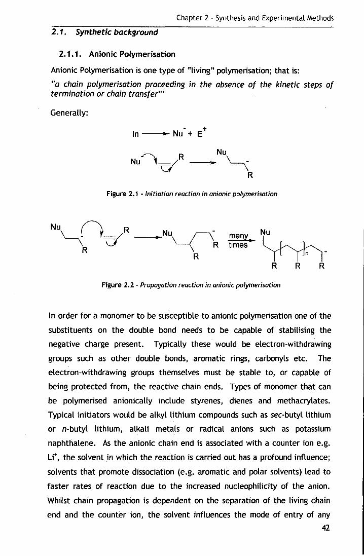
Chapter 2 - Synthesis and Experimental Methods
2.1. Synthetic background
2. 1. 1. Anionic Polymerisation
Anionic Polymerisation is one type of "living" polymerisation; that is:
"a chain polymerisation proceeding in the absence of the kinetic steps of termination or chain transfer" 1
.
Generally:
+ In _ ___,~ Nu + E
-~ R Nu .,~
Nu
~ R
Figure 2.1 -Initiation reaction in anionic polymerisation
many l h. ~ times • "(l ']1• "r
R R R
Figure 2.2- Propagation reaction in anionic polymerisation
In order for a monomer to be susceptible to anionic polymerisation one of the
substituents on the double bond needs to be capable of stabilising the
negative charge present. Typically these would be electron-withdrawing
groups such as other double bonds, aromatic rings, carbonyls etc. The
electron-withdrawing groups themselves must be stable to, or capable of
being protected from, the reactive chain ends. Types of monomer that can
be polymerised anionically include styrenes, dienes and methacrylates.
Typical initiators would be alkyl lithium compounds such as sec-butyl lithium
or n-butyl lithium, alkali metals or radical anions such as potassium
naphthalene. As the anionic chain end is associated with a counter ion e.g.
u+, the solvent .in which the reaction is carried out has a profound influence;
solvents that promote dissociation (e.g. aromatic and polar solvents) lead to
faster rates of reaction due to the increased nucleophilicity of the anion.
Whilst chain propagation is dependent on the separation of the living chain
end and the counter ion, the solvent influences the mode of entry of any
42
Chapter 2 - Synthesis and Experimental Methods
incoming monomer. Thus careful consideration should be given to
solvent/initiator combination due to the dramatic effect that can be achieved
with regards to the stereochemistry of the resulting polymer. Common
solvents used for the polymerisation of styrenes and dienes include benzene,
tetrahydrofuran (THF) and diethyl ether.
Anionic polymerisations are sensitive to trace quantities of impurities
including water, oxygen and carbon dioxide. These impurities may partidpate
in the polymerisation in a number of ways but the most influential process is
the termination or "killing" of living chains leading to loss of control. Thus
''clean" conditions are therefore necessary; one way of achieving such
conditions is through the use of high vacuum techniques.
A distinct advantage of anionic polymerisations is the ability to replace
hydrogen with deuterium without discernable affect on the polymerisability of
a monomer, meaning that deuterated polymers can be prepared that can
subsequently be utilised in neutron scattering experiments.
2.1.2. Why Use Anionic Polymerisation?
As previously mentioned, anionic polymerisation can be considered "living",
affording control over the major variables affecting the polymer properties,
namely molecular weight, molecular weight distribution, molecular
architecture, stereochemistry and copolymer composition.
2.1.2.1. Molecular weight
This is probably the single most important variable affecting polymer
properties. In anionic polymerisation, as with all living polymerisations, the
molecular weight is controlled by the stoichiometry of the reaction and the
degree of conversion. For a monofunctional initiator under ideal conditions
one polymer chain is formed per initiating molecule. At complete conversion,
the expected number average molecular weight can be calculated using
equation 2.1 2
M = monomer mass n initiator moles
Equation 2. 1
43
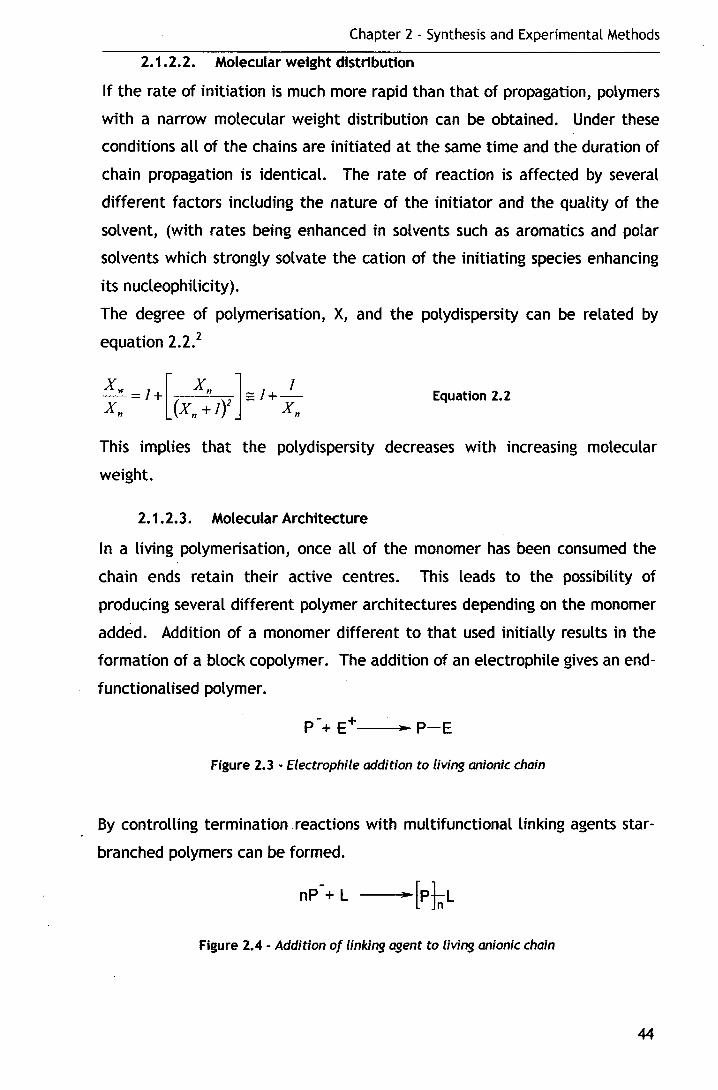
Chapter 2 - Synthesis and Experimental Methods
2.1.2.2. Molecular weight distribution
If the rate of initiation is much more rapid than that of propagation, polymers
with a narrow molecular weight distribution can be obtained. Under these
conditions all of the chains are initiated at the same time and the duration of
chain propagation is identical. The rate of reaction is affected by several
different factors including the nature of the initiator and the quality of the
solvent, (with rates being enhanced in solvents such as aromatics and polar
solvents which strongly solvate the cation of the initiating species enhancing
its nucleophilicity).
The degree of polymerisation, X, and the polydispersity can be related by
equation 2.2. 2
Equation 2.2
This implies that the polydispersity decreases with increasing molecular
weight.
2.1.2.3. Molecular Architecture
In a living polymerisation, once all of the monomer has been consumed the
chain ends retain their active centres. This leads to the possibility of
producing several different polymer architectures depending on the monomer
added. Addition of a monomer different to that used initially results in the
formation of a block copolymer. The addition of an electrophile gives an end
functionalised polymer.
Figure 2.3 - Electrophile addition to living anionic chain
By controlling termination .reactions with multifunctional linking agents star
branched polymers can be formed.
Figure 2.4 - Addition of linking agent to living anionic chain
44

Chapter 2 - Synthesis and Experimental Methods
2.1.2.4. Stereochemistry
Anionic polymerisation allows stereospecific polymers to be synthesised from
monomers where there is more than one possible mode of addition by careful
choice of the solvent/initiator combination. For example in the case of 1,3
butadiene three modes of addition are possible, 1,2 addition, cis 1,4 addition
and trans 1,4 addition. The proportions in which they are obtained are
influenced greatly by the solvent and counter ion. 3• 4 Different stereoisomers
of the same polymer can have vastly different properties. For example in the
case of poly(butadiene) the 1,2 stereoisomer has a glass transition
temperature of 258K, whereas the two 1 ,4 isomers cis and trans have glass
transition temperatures of 218 and 170K respectively. 5
2.2. Synthetk strategy
Two different molecular weight series of poly(butadiene)-poly(ethylene oxide)
block copolymers were synthesised, one of which was approximately 5000
gmol·1, the other being approximately 10000 gmol·1
• Each series had the same
molecular composition of approximately 15wt% poly(butadiene), and all Hand
D variants of the two blocks were to be synthesised, with the polybutadiene
block having a mainly 1,2 microstructure to facilitate post-polymerisation
cross-linking.
The synthesis of poly( ethylene oxide) block copolymers is complicated by the
lack of reactivity of ethylene oxide in the presence of a lithium counter ion
due to the formation of a strong ion pair between the active chain end and
the u+ counter ion. 6• 7 As a result even in large excesses of ethylene oxide
(EO) only one EO unit adds to the end of the active chain.
Bywater et al. 3 investigated the effect of solvent and counter ion on the
microstructure of poly(butadiene). They found that a lithium counter ion in
THF at temperatures less than 273K gave 1 ,2 content of the order of 90%. lt
was also interesting to note that the use of potassium in the same solvent at
similar temperatures resulted in polymers having almost 70% 1 ,2
microstructure. These results are in contrast to those of Milner and Young4
who showed that carrying out the same reaction in benzene at room
45

Chapter 2 - Synthesis and Experimental Methods
temperature with a lithium counter ion produced polymers with a majority of
1,4 microstructure.
2.2.1. Literature Procedures
Poly(butadiene)-poly(ethylene oxide) (PB-PEO) block copolymer syntheses
have been reported in the literature, the earliest of which was by Hillymer
and Bates in 1996.8 Although they did not directly synthesise poly(butadiene )
b/ock-poly(ethylene oxide) (the poly(butadiene) was hydrogenated in the
presence of a Palladium catalyst) the method was subsequently used to
produce poly(butadiene )-poly( ethylene oxide) block copolymers. 9
The polymerisation of 1,3 butadiene in THF at 223 to 213K using t-butyl
lithium or sec-butyl lithium initiator, resulted in a polymer that was end
capped by the addition of excess ethylene oxide, with the polymeric alcohol
isolated upon addition of methanolic HCl. The alcoholic polymer was titrated
with potassium naphthalenide, resulting in the potassium salt of the polymer,
which initiated the eo-polymerisation of ethylene oxide. Under these reaction
conditions, formation of the 1,2 isomer of PB predominates, with polymers
containing on average 90% 1,2 units (scheme 2.1 ).
0 1)L_i208K-RT ~OH
R-li + f\ THF, 213K, 4.5hr ~- R --- hydrogenation 2)H+,RT ~
.b-
THF, RT
1)~ THF, 318K, 20hr
2)H+
Scheme 2. 1- Reaction scheme of Hillmyer and Batet
Hoerner · et al. 10 (scheme 2.2) used cumyl potassium to initiate the
polymerisation of butadiene in THF at 213K, followed by the addition of
46
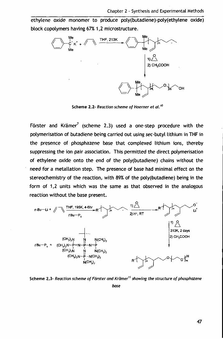
Chapter 2 - Synthesis and Experimental Methods
ethylene oxide monomer to produce poly(butadiene)-poly(ethylene oxide)
block copolymers having 67% 1,2 microstructure.
2) CHsCOOH
Scheme 2.2- Reaction scheme of Hoerner et al. 10
Forster and Kramer7 (scheme 2.3) used a one-step procedure with the
polymerisation of butadiene being carried out using sec-butyl lithium in THF in
the presence of phosphazene base that complexed lithium ions, thereby
suppressing the ion pair association. This permitted the direct polymerisation
of ethylene oxide onto the end of the poly(butadiene) chains without the
need for a metallation step. The presence of base had minimal effect on the
stereochemistry of the reaction, with 89% of the poly(butadiene) being in the
form of 1,2 units which was the same as that observed in the analogous
reaction without the base present.
0 n Bu-Li + ~ THF, 195K, 4-6hr R~ _1)_u ___ .__,R~~:
tBu-P4
~ 2) H+, RT ~ ~
tBu-P4 =
1) 3,. 3131<, 2 days
2) CH3COOH
Scheme 2.3- Reaction scheme of Forster and Kri:imer11 showing the structure of phosphazene
base
47
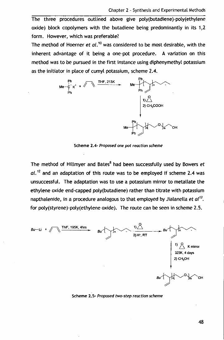
Chapter 2 - Synthesis and Experimental Methods
The three procedures outlined above give poly(butadiene)-poly(ethylene
oxide) block copolymers with the butadiene being predominantly in its 1 ,2
form. However, which was preferable?
The method of Hoerner et al. 10 was considered to be most desirable, with the
inherent advantage of it being a one-pot procedure. A variation on this
method was to be pursued in the first instance using diphenymethyl potassium
as the initiator in place of cumyl potassium, scheme 2.4.
~~ + ~ THF,213K Me-C K + 'I \
I Ph
Me~. 0
1)u
2)C~COOH
Ph
Me~0~0H ~h ~
Scheme 2.4- Proposed one pot reaction scheme
The method of Hillmyer and Bates8 had been successfully used by Bowers et
al. 12 and an adaptation of this route was to be employed if scheme 2.4 was
unsuccessful. The adaptation was to use a potassium mirror to metallate the
ethylene oxide end-capped poly(butadiene) rather than titrate with potassium
napthalenide, in a procedure analogous to that employed by Jialanella et al 13•
for poly(styrene)-poly(ethylene oxide). The route can be seen in scheme 2.5.
Bu-Li + ~ THF, 195K, 4hrs 0
Bu~ -1>_D ___ _.Bu~ _) 2)H+, RT _)
1) 0 . 0 Kllllrror
Scheme 2. 5- Proposed two-step reaction scheme
323K, 4 days
2)C~OH
48

Chapter 2 Synthesis and ExoL~rimental Methods
2.2.2. Cross-linking reactions
Block copolymer micelles dispersed in selective solvents are not permanent
structures 14 and the unsaturation of the poly(butadiene) in the copolymers
synthesised as part of this research was to be exploited to cross-link the cores
rendering the micelles permanent structures. This is shown schematically in
figure 2.5.
Selective
Solvent
Permanent structure
Figure 2.5 - Schematic representation of cross-linked micelles
Because aqueous dispersions of micelles were desired, common free-radical
initiators were unsuitable because of their insolubility in water. Additionally
to preserve the structure of the micelle the use of initiators that required
elevated temperature was also prohibited.
Several groups have used photo initiators in conjunction with UV light to
generate free-radicals and cross-link micelles having a poly(butadiene) core.
Tuzar et al. 15 utHised dibenzoyl peroxide as a photo initiator to cross-link
poly(butadiene)-poly(styrene) micelles in THF /ethanol dispersions. Wilson
and Riess 16 used benzoin ethyl ether to cross-link the micelles of the same
polymer but this time in DMF. Both of the methods are relatively straight
forward, but require the use of quartz vessels to transmit the UV light.
A redox initiator system often used for free-radical polymerisation was
thought to be the most appropriate. Redox initiators can be used in aqueous
conditions at room temperature using combinations of inorganic salts to 49

Chapter 2 SyntheSlS and Expenmental Methods
generate free radicals at an acceptable rate .17 Bates and eo-workers have
used this method to cross-link poly(butadiene)-poly(ethylene oxide) micelles
in aqueous solution. 9• 18
2.3. Synthetic procedures
2.3.1 . Block Copolymer synthesis
All of the reactions were carried out under high vacuum conditions using
''Christmas tree" type reaction vessels, which can be seen in figure 2.6.
Figure 2.6 - Single reaction bulb "Chr istmas-tree"
2.3.1.1. Materials
All materials were supplied by Aldrich Chemicals unless stated otherwise.
Tetrahydrofuran (THF) (250ml) was purified via. degassing over sodium wire
and benzophenone. Ethylene oxide was vacuum distilled onto potassium
hydroxide contained in a 50ml reaction flask that was partially immersed in
iced water, and the EO/ KOH mixture stirred for 15hrs. The monomer was
then vacuum distilled into a flask containing calcium hydride and degassed
several times by free-evacuate-thaw cycles. The flask was again immersed in
iced water and stirred for ea. 15hrs. After vacuum transfer to a new flask,
dibutyl magnesium (1 ml) was injected for final purification. The deuterated
ethylene oxide (Fluka) was treated in the same manner as the hydrogenous
version, with the omission of the potassium hydroxide step.
Butadiene was purified by passing through a series of columns fllled with
different grades of molecular sieves to remove any moisture.
50
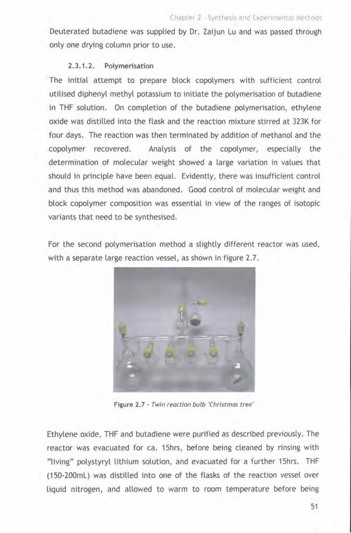
Chapter 2 Synthesis and Exoenmental Methods
Deuterated butadiene was supplied by Dr. Zaijun Lu and was passed through
only one drying column prior to use.
2.3.1.2. Polymerisation
The initial attempt to prepare block copolymers with sufficient control
utilised diphenyl methyl potassium to initiate the polymerisation of butadiene
in THF solution. On completion of the butadiene polymerisation, ethylene
oxide was distilled into the flask and the reaction mixture stirred at 323K for
four days. The reaction was then terminated by addition of methanol and the
copolymer recovered. Analysis of the copolymer, especially the
determination of molecular weight showed a large variation in values that
should in principle have been equal. Evidently, there was insufficient control
and thus this method was abandoned. Good control of molecular weight and
block copolymer composition was essential in view of the ranges of isotopic
variants that need to be synthesised.
For the second polymerisation method a slightly different reactor was used,
with a separate large reaction vessel, as shown in figure 2. 7.
Figure 2. 7 - Twin reaction bulb "Chr istmas tree"
Ethylene oxide, THF and butadiene were purified as described previously. The
reactor was evacuated for ea. 15hrs, before being cleaned by rinsing with
"living" polystyryl lithium solution, and evacuated for a further 15hrs. THF
(150-200ml) was distilled into one of the flasks of the reaction vessel over
liquid nitrogen, and allowed to warm to room temperature before being
51
Chapter 2 - Synthesis and Experimental Methods
stirred. Butadiene (2. 99g) was distilled into the reaction vessel immersed in a
solid COdacetone bath, followed by injection of sec-butyl lithium
(0.00199mol, 1.4ml) initiator solution, which caused the solution to turn
yellow in colour. The reaction was stirred at 195K for 4hrs, before adding
ethylene oxide (1g) to end-cap the living poly(butadiene) chains, and stirred
for a further 2hrs (when a sample of the reaction mixture (10-15ml) was
decanted into a side arm flask and terminated with degassed methanol
(O.Sml)) The main mass of the reaction mixture was also terminated by
injecting degassed methanol (1 ml). The solvent was distilled out of the flask
to leave a slightly opaque white oil. Fresh THF (150ml) was distilled onto the
copolymer cooled by immersing the flask in a C02/ acetone bath. The polymer
solution was left stirring for 2hrs before the solvent was distilled out again
leaving behind the oily polymer, which was pumped on at high vacuum for 2
days. More THF (150-200ml) was distilled onto the cooled polymer (195K) in
order to redissolve it prior to the metallation. Potassium (0.00995mol, 0.4g)
was cleaned in hexane and added to the unused flask of the vessel whilst a
flow of dry nitrog~n through the flask was maintained. The flask was re
evacuated, and the potassium vaporised by gentle warming, with it
condensing on the cooler parts of the flask generating a mirror in snu. The
polymer solution from the first reaction vessel was decanted onto the mirror;
agitated periodically over two hours to ensure efficient metallation by the
potassium mirror, after which time the solution was decanted back to the first
flask. Ethylene oxide (16.29g) was distilled on to the cooled (195K) solution
which was stirred at room temperature for ea 15hrs, and then stirred at 323K
for three days, during which time a yellow colour developed. After cooling to
room temperature, degassed methanol (1ml) was injected to terminate the
reaction, followed by stirring for Y2hr. The polymer was recovered by
precipitation into stirred hexane (800ml), yielding a white solid, which was
dried at room temperature in vacuo. for 24hrs.
The identical synthesis procedure was applied to all the isotopic variants for
each molecular weight copolymer, these isotopic variants being hPB-hPEO,
dPB-hPEO and hPB-dPEO. (section 2.6 pg 70)
52

Chapter 2 - Synthesis and Experimental Methods
2.3.1.3. Polymer and copolymer characterisation
The poly(butadiene) block was characterised using size exclusion
chromatography (SEC or GPC) and 1H NMR; and the copolymer analysed by SEC
in THF, 1H NMR or 13C NMR depending on isotopic labelling, and differential
scanning· calorimetery (DSC)
NMR spectra were recorded using a Varian Mercury spectrometer operating at
399.97 MHz for 1H and 100.57 MHz for 13C. SEC data were obtained using
Viscotek 200 chromatograph equipped with refractive index, viscosity and
light scattering detectors using THF as the eluent. Poly(butadiene) blocks
were analysed using poly(butadiene) calibrants.
poly(styrene) standards were used as calibrants.
For the copolymers
DSC data were obtained using a Perkin Elmer Pyris 1 DSC and a heating rate of
2.3.2. Micelle core cross-linking
Attempts to cross-link the micelle cores using the redox couple of sodium
meta bisulphite, lron(ll) sulphate heptahydrate and tert-butylhydroperoxide
reported by McCarthy et al. 19 proved unsuccessful. The combination of
initiators proved not to be robust, with the reaction difficult to reproduce
upon scaling up.
Initial attempts at using the method reported by Won, Davis and Bates were
also unsuccessful in that although the micelles were cross-linked, upon their
recovery from the reaction mixture by freeze-drying, they were no longer
dispersible in water.
The method eventually settled upon was a slight variation of that used by Won
et. al. 9• 18 in that higher concentration dispersions were used, with samples
prepared by dilution directly from the reaction mixture.
An aqueous copolymer dispersion in D20 (10ml, 10%) was added to a 100ml
round-bottomed flask, having a septum, side arrr1 connector, and Young's tap,
which was stirred gently and sparged with nitrogen for 2hrs. Potassium
persulphate (10Wt%, 1g) was added to the polymer dispersion prior to stirring.
Initiator solutions were prepared in the same solvent as the polymer solution,
as detailed in table 2.1
53

Chapter 2 - Synthesis and Experimental Methods
Volume Amount Ratio to Initiator AmounUg
H20/ml Condwt% injected/ml
polymer mass
Sodium 2.00602 5 40 1.25 0.5 metabisulphite Iron (11) sulphate 1.58944 5 30 0.09 0.02
heptahydrate
Table 2. 1 - Quantities of initiators used
The initiator solutions were injected through the septum turning the solution
yellow in colour. After initial stirring the reaction was left quiescent for
15hrs, after which it was colourless. The solutions were diluted directly for
use in small-angle neutron scattering experiments using the appropriate
solvent. The product was characterised by 1H NMR in D20.
2.4. Experimental methods
2.4.1. Small-Angle Scattering Techniques
Small-angle X-ray and neutron scattering (SAXS and SANS respectively) are
simple diffraction techniques that exploit the wave-particle duality of the
respective radiation to provide information about the size and shape of
molecules and their interactions with each other.20'
21 Even though X-rays and
neutrons interact with different parts of the atom, electrons and nuclei
respectively, and are sensitive to inhomogeneities in different properties,
namely electron density and neutron scattering length density, the underlying
principles for both techniques are identical. The two techniques along with
static light scattering are complementary to each other yielding information
on different length scales. Table 2.2 provides an overview of the techniques,
and outlines the information obtainable from each. 20•
22
54
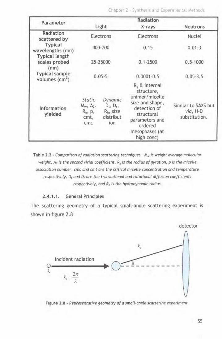
Chapter 2 Synthes1s and Experimental Methods
Parameter Radiation Light X-rays Neutrons
Radiation Electrons Electrons Nuclei
scattered by Typical
400-700 0.15 0.01-3 wavelengths (nm)
Typical length scales probed 25-25000 0.1-2500 0.5-1000
(nm) Typical sample volumes (cm3
) 0.05-5 0.0001-0.5 0.05-3.5
Rg & internal structure,
Static Dynamic unimer I micelle size and shape,
Information Mw, A2. Dt, Or,
detection of Similar to SAXS but
yielded Rg, p, Rh, size
structural via, H-0
cmt, distribut parameters and substitution.
erne ion ordered
mesophases (at high cone)
Table 2.2- Comparison of radiation scattering techniques. Mw is weight average molecular
weight, A2 is the second virial coefficient, R!l is the radius of gyration, p is the micelle
association number, erne and cmt are the critical micelle concentration and temperature
respectively, Dt and Dr are the translational and rotational d;ffusion coefficients
respectively, and Rh is the hydrodynamic radius.
2.4. 1. 1. General Prindples
The scattering geometry of a typical small-angle scattering experiment is
shown in figure 2.8
detector
Incident radiation
0-------~~· 0--]-------- -')...
k. = 2K I A
Figure 2.8- Representative geometry of a small-angle scattering experiment
55
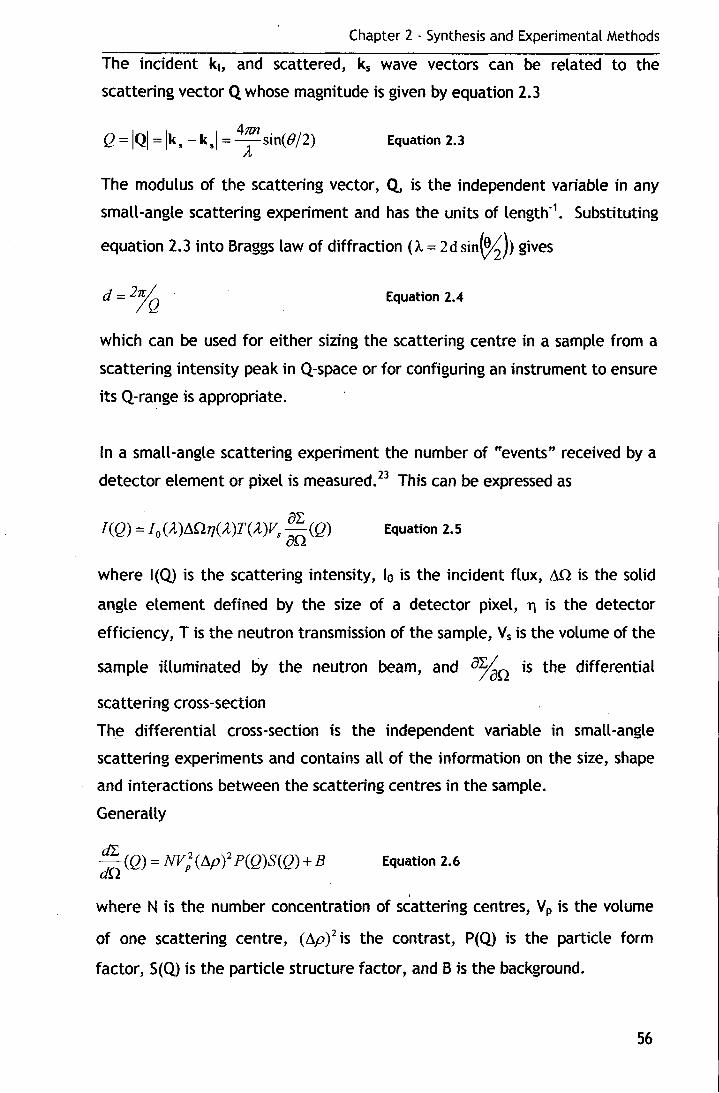
Chapter 2 - Synthesis and Experimental Methods
The incident k~, and scattered, ks wave vectors can be related to the
scattering vector Q whose magnitude is given by equation 2.3
Q = IQI = lk.-k.l = 4
1l1l sin(B/2) A.
Equation 2.3
The modulus of the scattering vector, Q, is the independent variable in any
small-angle scattering experiment and has the units of length-1• Substituting
equation 2. 3 into Braggs law of diffraction (A.= 2 d sin~)> gives
Equation 2.4
which can be used for either sizing the scattering centre in a sample from a
scattering intensity peak in Q-space or for configuring an instrument to ensure
its Q-range is appropriate.
In a small-angle scattering experiment the number of tfevents" received by a
detector element or pixel is measured. 23 This can be expressed as
Equation 2. 5
where I(Q) is the scattering intensity, 10 is the incident flux, 11Q is the solid
angle element defined by the size of a detector pixel, 11 is the detector
efficiency, T is the neutron transmission of the sample, Vs is the volume of the
sample illuminated by the neutron beam, and a%n is the differential
scattering cross-section
The differential cross-section is the independent variable in small-angle
scattering experiments and contains all of the information on the size, shape
and interactions between the scattering centres in the sample.
Generally
d'£ (Q) = NV:(L1p)2 P(Q)S(Q)+ B dQ
Equation 2.6
where N is the number concentration of scattering centres, Vp is the volume
of one scattering centre, (11p) 2 is the contrast, P(Q) is the particle form
factor, S(Q) is the particle structure factor, and B is the background.
56

Chapter 2 - Synthesis and Experimental Methods
2.4.1.2. Contrast
In order to be able to obtain scattering from a system there must be a degree
of contrast present; that is the property governing the interaction with the
incident radiation must be different in the scattering body to that of its
surroundings. If this is not the case then the system is said to be at contrast
match and no scattering is observed. In SAXS the contrast arises from the
electron density difference and in SANS from the neutron s~attering length
density difference. Table 2.3 shows the atomic scattering lengths and
neutron scattering lengths for some common atoms and their isotopes for both
X-rays and neutrons. 24
Element X-ray scattering length/10-12cm
0.282 0.282 1.41 1.69 1.97
. 2.26
Neutron coherent scattering lengths/10"12cm
-0.374 0.667 0.54
0.665 0.94 0.580
·Table 2.3 - Comparison of x-ray and neutron scattering lengths for common atomic species
As can be seen from table 2.3 the variation of the atomic scattering lengths
for neutrons varies somewhat irregularly with atomic number. This is not the
case for X-rays, where the X-ray scattering length scales with increasing
number of electrons, thus increasing linearly with atomic number. Of
particular significance is the difference in . both sign and magnitude for
hydrogen and deuterium scattering lengths. This allows manipulation of the
scattering length by replacing hydrogen with deuterium in a molecule and is
thus highly relevant for small angle neutron scattering.
The scattering length density of a molecule is obtained using equation 2.7.20'
25
Equation 2. 7
For polymers it is only necessary to calculate the scattering length or electron
density for one repeat unit, since these are the scattering centres.
57
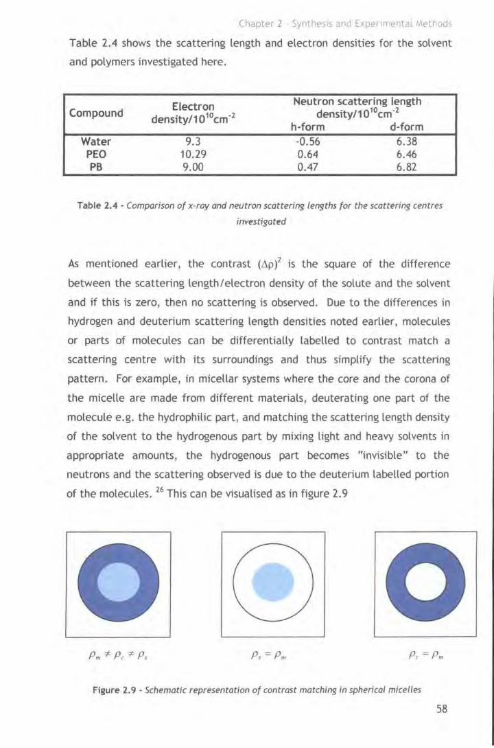
Chapter 2 Syntht?SlS and Experunental Methods
Table 2.4 shows the scattering length and electron densities for the solvent
and polymers investigated here.
Compound
Water PEO PB
Electron density/1010cm·2
9.3 10.29 9.00
Neutron scattering length density/1010cm·2
h-form d-form -0.56 6.38 0.64 6.46 0.47 6.82
Table 2.4 - Comparison of x-roy and neutron scattering lengths for the scattering centres
investigated
As mentioned earlier, the contrast (6p )2 is the square of the difference
between the scattering length/electron density of the solute and the solvent
and if this is zero, then no scattering is observed. Due to the differences in
hydrogen and deuterium scattering length densities noted earlier, molecules
or parts of molecules can be differentially labelled to contrast match a
scattering centre with its surroundings and thus simplify the scattering
pattern. For example, in micellar systems where the core and the corona of
the micelle are made from different materials, deuterating one part of the
molecule e.g. the hydrophilic part, and matching the scattering length density
of the solvent to the hydrogenous part by mixing light and heavy solvents in
appropriate amounts, the hydrogenous part becomes "invisible" to the
neutrons and the scattering observed is due to the deuterium labelled portion
of the molecules. 26 This can be visualised as in figure 2. 9
Ps =Pm
Figure 2. 9 - Schematic representation of contrast matching in spherical micelles
58

Chapter 2 - Synthesis and Experimental Methods
As was noted in section 2.3.1.2 per-deuterated analogues of the block
copolymers were synthesised by using anionic polymerisation.
2.4.1.3. Form Factor
The form factor (P(Q) in equation 2.6) describes how dlYdQ(Q) is modulated
by interference effects between radiation scattered from different parts of
the same scattering particle. Consequently it is sensitive to the size and
shape of the scattering particles. Analytical expressions for P(Q) exist for
many particle morphologies, a large number of which have been set out by
' Pedersen. 27 Perhaps the most common is that of a uniform sphere, equation
2.8, derived by Lord Rayleigh in 1911.28
P(Q) = [3(sin(QR)- QRcos(QR))]2
QR3 Equation 2.8
For solutions of spherical micelles the form factor of a sphere is not
appropriate because the micelle consists of two concentric spheres, that of
the poorly solvated component surrounded by a second of the well solvated
component, shown schemati~ally in figure 2.1 0. In this case a core-shell
model for P(Q) would be used.20•
29
Pm
Figure 2.10- Schematic representation of a core-shell particle. R, is the core radius, Res is
the micelle radius, pis the scattering length density, where subscript c implies the core, s
implies the shell and m the solvent.
59
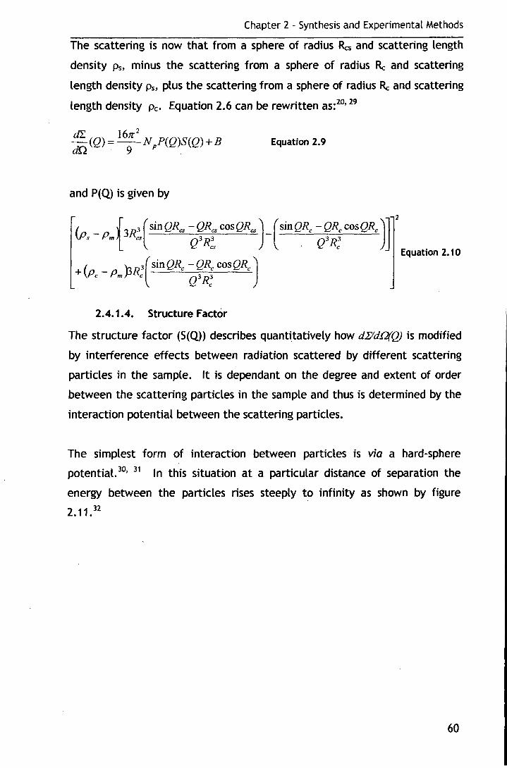
Chapter 2 - Synthesis and Experimental Methods
The scattering is now that from a sphere of radius Res and scattering length
density Ps, minus the scattering from a sphere of radius Re and scattering
length density Ps, plus the scattering from a sphere of radius Re and scattering
length density Pc· Equation 2.6 can be rewritten as: 20'
29
dL (Q) = 16Jr2 N P(Q)S(Q) + B dQ 9 p .
Equation 2. 9
and P(Q) is given by
2.4. 1.4. Structure Factor
The structure factor (S(Q)) describes quantitatively how d.Eid.Q(Q) is modified
by interference effects between radiation scattered by different scattering
particles in the sample. lt is dependant on the degree and extent of order
between the scattering particles in the sample and thus is determined by the
interaction potential between the scattering particles.
The simplest form of interaction between particles is via a hard-sphere
potential. 30'
31 In this situation at a particular distance of separation the
energy between the particles rises steeply to infinity as shown by figure
2. 11.32
60
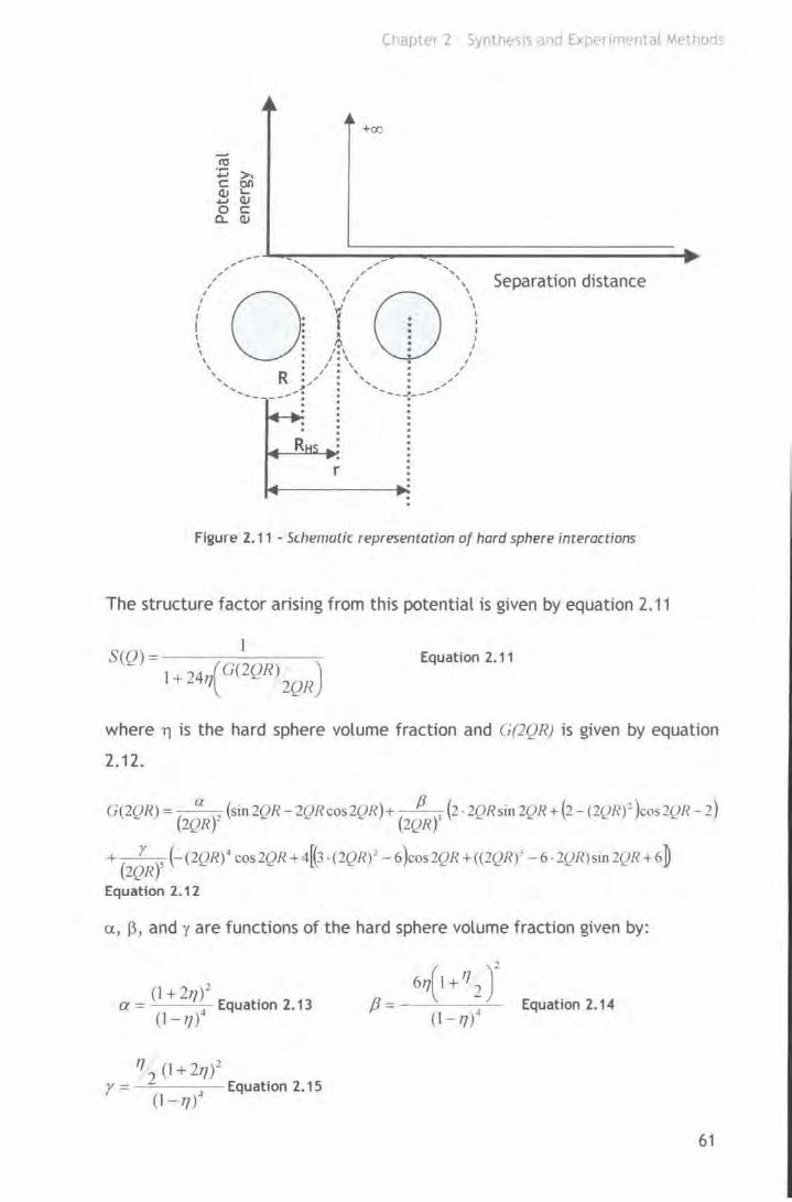
Chapter 2 Synthesis .ancf Expe11r11ental Methods
+oo
, ,-- ... , , , -... , '
, ... ' ,
' /
Separation distance I ' / ' I I \
' I ' I
0 I I
0 I I
I I¥! \ I f
I
I I I
I ~ I I r,. I I 1,1 I I I • \ I
' . I . ' . I
' R . I . ' . I
' ;.-.. . ' . .. ... : ' , ... ... '---:--~' - ---': . . . . . .
r
Figure 2. 11 - Schematic representation of hard sphere interactions
The structure factor arising from this potential is given by equation 2.11
S(O) = I - I+ 2417(G(2QR) )
2QR
Equation 2. 11
where 11 is the hard sphere volume fraction and (;(2QRJ is given by equation
2.12.
U(2QR)= ( aY (sin2QR-2QRcos2tJR)+ ( fJ 1 (2 ·20Rsm2QR+(2-(2{_)R)")cos2(JR-2) 2QR 2QR)· -
+ (2;RY (-(2QR)
4 cos2QR+4((3 ·(2QR) 2 -6)cos2QR+((2QR)' -6·2QR)sin2{!R+6D
Equation 2.12
a, (3, and 'Y are functions of the hard sphere volume fraction given by:
(1 + 2t7)2 a =
4 Equation 2. 13
(l-f,7)
17 (1 + 277/ y = 2 ~ Equation 2. 1 5
(l-7])
61

Chapter 2 - Synthesis and Experimental Methods
2.4.2. Light scattering
Light scattering is a non-invasive, non-destructive technique that can be
utilised for the characterisation of complex fluids such as polymer solutions. 33
Light incident on a solution of molecules gives rise to scattering by virtue of
the interaction of its electric field with the electrons of the molecules in
solution. 34 These molecules are in constant random motion, Brownian motion,
and so on a microscopic scale cause density fluctuations in the solution.
These density fluctuations cause a small shift in the frequency of the
scattered light relative to that of the incident frequenc~5 and the process is
said to be quasi-elastic, hence the name quasi-elastic light scattering (QELS)
given to this form of study. As the movements of the molecules are very fast
it is possible to collect scattered light in time periods sufficiently longer than
those associated with the movements of the molecules, giving an average over
the number of particles in the scattering volume. In this instance the
frequency shift is not observed and the process is said to be elastic. This
technique is known as static or classical light scattering (SLS).
The two scattering processes yield complementary information for the
scattering molecules; static light scattering provides information on the
molecular weight, radius of gyration and thermodynamics of interaction with
the solvent, whilst quasi-elastic light scattering yields diffusion coefficients
from which size parameters can be obtained. Each of the two techniques will
be discussed in turn.
2.4.2.1. Static Light scattering33•
34•
36•
37
The size of a molecule has a profound effect on its scattering properties and
the key parameter is the molecular size relative to the wavelength of the
incident light. If the molecular dimensions are less than 'A/20 the molecule
can be considered as a point scatterer; i.e. a Rayleigh scatterer. Those
particles with dimensions comparable to the incident wavelength are large;
i.e. Debye scatterers.
When d<A./20 the intensity of light scattered from a dilute solution of polymer
molecules consists of two contributions:
i.) Intensity due to density fluctuations of the solvent
ii.) Intensity due to the scattering from concentration fluctuations of the
polymer molecules
62
Chapter 2 - Synthesis and Experimental Methods
The presence of small amounts of polymer molecules has little effect on the
density fluctuations, and so two scattering intensities have to be measured,
that of the pure solvent and of the polymer solution. The difference in the
two intensities is the contribution from the dissolved polymer molecules to
the overall intensity, which is referred to as the excess scattering.
If the polymer molecules can be considered to be independent of one
another, i.e. in dilute solution, then the scattering intensity from that
solution at an angle 8 to the incident beam is given by equation 2.16
2 2 ( )2 I = I 41r no dn Me e o 2 14N .-~
r.~~,0 A uc Equation 2. 16
where le is the intensity of polarised light scattered from a dilut.e polymer
solution at angle 8, lo is the incident light intensity, n0 is the solvent
refractive index, r is the distance between the scattering molecule and the
detector, A.o is the incident wavelength radiation, NA is Avogadro's number,
d'Jdc is the specific refractive index increment, M is the molecular weight of
the polymer and c is its concentration.
The specific refractive index increment, dn/dc, is the change in refractive
index of a dilute polymer solution for a unit increase in the concentration of
the polymer, the units are customarily ml g·1•
The increase in scattered intensity from a solution in relation to the pure
solvent is due to fluctuations in the solute concentration within small volume
elements, the dimensions of which are such that they can be considered point
scatterers in relation to the incident wavelength; they must also be large
enough to hold many solvent and a few solute molecules. As a result of the
number of solute molecules within a volume element changing concentration
fluctuations occur. Allowing for these concentration fluctuations the
scattered intensity is now given by:
Equation 2. 17
Often measurements are performed in solutions sufficiently dilute that the
third and higher virial coefficients are negligible and can be discarded.
63

Chapter 2 - Synthesis and Experimental Methods
Equation 2.17 can be re-written as:
Equation 2. 18
Equation 2. 19
Re is the Rayleigh ratio, which is a measure of reduced intensity of scattered
light at any angle to the incident beam, and is independent of the instrument.
Jt eliminates intensity changes due to the angular dependence of scattering
intensity upon the degree of polarisation of the incident beam and on the
parameters of the apparatus.
If the dimensions of the solute are greater than 'A/20, then light scattered
from different parts of the molecule is coherent and capable of interference,
with the beams reaching the detector with different phases potentially
resulting in an intensity which is reduced in comparison to the sum of the
intensities of the constituent beams. As the light is scattered from different
parts of the same molecule, the effect is one of intramolecular interference.
As a result of this interference, the intensity of scattered light depends upon
the angle of observation. , This angular dependence can be described by the
particle scattering factor P(()), which can be defined as the Rayleigh ratios at
the angle of observation B, and at zero angle_, i.e. P(B) =RI{ . P(()) is
analogous to P(Q) in small angle scattering, and is characteristic of molecular
shape.
From this definition, P(O)= 1 for particles of any size and shape. For small
particles P(())=l at any angle as the Rayleigh ratio is independent of the angle
of observation under this condition.
The basic equation given earlier· for light scattering from dilute polymer
solutions with small dimensions compared to the incident wavelength is only
valid for large polymers when B equals zero, as there is no reduction in the
scattered intensity due to intramolecular interference. Thus
64
Chapter 2 - Synthesis and Experimental Methods
Equation 2. 20
butRo = R~(B), so substituting this into equation 2.20 gives
Equation 2. 21
which is the classical form .of equation for static light scattering from polymer
molecules presented by Zimm.
P(S) can be related to the radius of gyration by equation 2.22
_l_=l-16Jr2 (R2)sin2((}/) P(B) 311? g \/2 Equation 2.22
substituting equation 2.22 into 2.21 gives
Equation 2. 23
Equation 2.23 can be used to determine the molecular weight, radius of
gyration and second virial coefficient from a plot of Kc/Re vs. sin2(812)+kc
where k is a plotting constant via a double extrapolation procedure (see
section 3.4).
2.4.2.2. Quasi-elastic Light Scattering33•
35•
38
The Brownian motion of polymer molecules in solution gives rise to density
fluctuations on a microscopic scale that appear and disappear at a rate
determined by the speed of the molecules' Brownian motions.
Quasi-elastic light scattering allows measurement of the density fluctuations
as a function of time to yield information about the diffusion coeffidents
from which molecular size can be obtained. This is achieved via. the intensity
autocorrelation function, g(t), equation 2.24
00
g(t) = f I(t).I(t+T)dt Equation 2.24 0
where I(t) is the intensity of scattered light at time t, and .I(t+ T) is the
intensity of scattered light at time t+ r:
65
Chapter 2 - Synthesis and Experimental Methods
For a system of hard, spherical, non-interacting particles in a fluid the
correlation function, g(T), is given by
g(r) = exp(-rt) Equation 2.25
The relaxation rate, r, is related to the scattering vector, Q, and the
diffusion coefficient, D, by:
4mz · Q = -sin(0/2)
A-
Equation 2.26
Equation 2.27
The relaxation rate can be obtained by fitting the experimental correlation
data to one of several models and since Q is known, the diffusion coefficient
can be calculated. The diffusion coefficient can be used to determine the
hydrodynamic radius, Rh, using the Stokes-Einstein equation
Equation 2.28
where ks is Boltzmann's constant, T is the temperature and 11 is the solvent
viscosity.
Often, for a monodisperse or highly dilute sample, a simple exponential fit is
sufficient to extract the relaxation· rate from the correlation function.
Sometimes however, polydisperse or more concentrated samples are
examined and the correlation function can no longer be expressed by equation
2.25. The autocorrelation now has the form of a distribution of exponentials
expressed as a Laplace integral:
00
g('r) = J G(r)e-rT dr Equation 2.29 0
There are several methods of analysing correlation functions of polydisperse
or non-dilute systems with two of the most common being the cumulants39
and CONTIN40 methods.
In the cumulants39 method a Taylor series expansion of the logarithm of
equation 2.29 is used to average over all of the light scattering particles, i.e.
K r 2
lng(r)=-K1r+-2 -+ ... 2
Equation 2.30
where K1 and K2 are the first and second cumulants respectively. 66
Chapter 2 - Synthesis and Experimental Methods
The cumulants of the expansion give the average diffusion coefficient and the
normalised distribution width for the first and second cumulants respectively.
Higher cumulants are not usually justifiable due to the quality of the data.
In the CONTIN40 method, g(t) is represented by a series of discrete steps, each
of width ,1.r. In this instance g(t) is given by equation 2.31.
Equation 2.31
The step width and number of steps are varied until a best fit is obtained.
2.5. Experimental procedures
2.5.1. Specimen preparation
2.5.1.1. Dispersion Preparation
All glassware was cleaned using permanganic acid prior to use to remove any
impurities adhering to the glass surface. Potassium Permanganate (ea.
100mg) was dissolved in concentrated sulphuric acid (200ml) producing a pale
green viscous liquid. The acid was poured into any glassware to be cleaned
and left overnight, after which it was rinsed with ultra high quality water,
followed by ethanol and then dried in vacuo at room temperature.
Aqueous dispersions were prepared by mixing a known weight of the
copolymer with an appropriate volume of UHQ water, and/or heavy water
(Aldrich, 99.9% inclusion), and leaving in the dark for several days to
equilibrate.
2.5.2. Light Scattering measurements
Light scattering measurements were performed at the universities of Durham
and Sheffield on apparatus equipped with either a Laser Quantum Torus 532
(Durham) or a Uniphase microgreen (Sheffield) frequency doubled Nd-YAG
laser with an incident wavelength of 532nm. These were both used in
conjunction with a Brookhaven BI200SM goniometer coupled to either an
avalanche photo diode (Durham) or a photo multiplier tube (Sheffield), with
the outputs measured by a Brookhaven BI9000AT digital autocorrelator.
67
Chapter 2 - Synthesis and Experimental Methods
All of the dispersions were filtered several times through a cellulose ester
filter (Millipore), having a pore size of 0.22~-tm, in order to remove dust
particles.
Quasi-elastic light scattering measurements were carried out at an angle of
90° to the incident beam and results presented are the averages of several
repeated runs.
Static light scattering measurements were performed over the angular range
30s;es;150°.
The specific refractive index increment of the copolymer dispersions was
determined using a Brice-Phoenix differential refractometer. The difference
in refractive index between a copolymer dispersion and the pure solvent was
determined for a series of solutions ranging in concentration from 0. 5 to 2% at
four wavelengths between 436 and 633nm. A plot of refractive index change
vs. concentration for each wavelength gave the dn/dc value for the respective
wavelength, with these being plotted against 1 /wavelength2 to give the
wavelength dependence of dn/dc. The procedure was repeated for solutions
of the polymer in chloroform, which is a good solvent for both blocks of the
copolymer.
2.5.3. Small-Angle X-ray Scattering
SAXS data were obtained using a Kratky compact camera equipped with a
Braun 50M position sensitive wire detector with 1024 position sensitive
channels. The X-ray generator was operated at 25mA and 25kV using CuKa
radiation. All of the measurements were performed in vacuo. Liquid samples
were housed in a quartz capillary tube.
Data were the result of repeated runs averaged and corrected for both sample
transmission and background scattering. Use was made of the ITR41 software
to desmear the raw data to correct for the influence of a finite slit width.
68
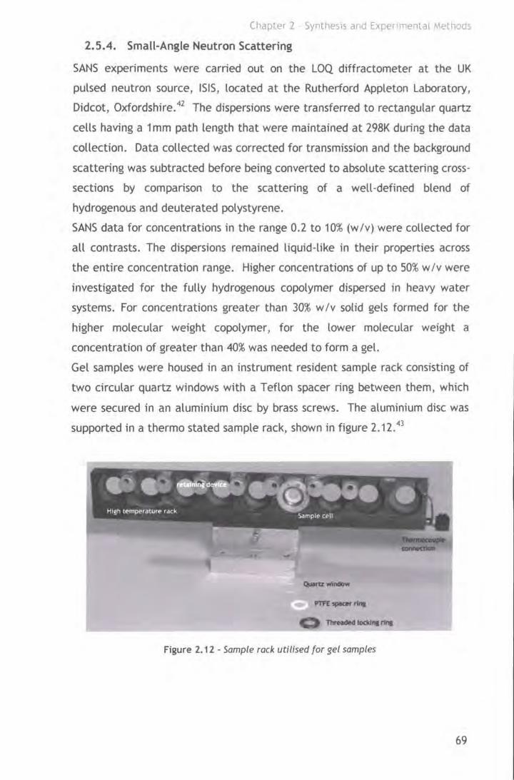
Chapter 2 Symhesis and Exper 1mental Methods
2.5.4. Small-Angle Neutron Scattering
SANS experiments were carried out on the LOQ diffractometer at the UK
pulsed neutron source, ISIS, located at the Rutherford Appleton Laboratory,
Didcot, Oxfordshire. 42 The dispersions were transferred to rectangular quartz
cells having a 1 mm path length that were maintained at 298K during the data
collection. Data collected was corrected for transmission and the background
scattering was subtracted before being converted to absolute scattering cross
sections by comparison to the scattering of a well-defined blend of
hydrogenous and deuterated polystyrene.
SANS data for concentrations in the range 0.2 to 10% (w /v) were collected for
all contrasts. The dispersions remained liquid-like in their properties across
the entire concentration range. Higher concentrations of up to 50% w/v were
investigated for the fully hydrogenous copolymer dispersed in heavy water
systems. For concentrations greater than 30% w /v solid gels formed for the
higher molecular weight copolymer, for the lower molecular weight a
concentration of greater than 40% was needed to form a gel.
Gel samples were housed in an instrument resident sample rack consisting of
two circular quartz windows with a Teflon spacer ring between them, which
were secured in an aluminium disc by brass screws. The aluminium disc was
supported in a thermo stated sample rack, shown in figure 2.12:13
Figure 2.12 • Sample rack utilised for gel samples
69
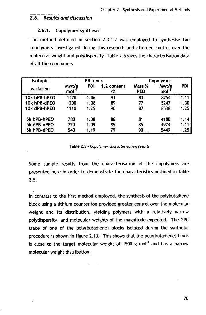
Chapter 2 - Synthesis and Experimental Methods
2.6. Results and discussion
2.6.1. Copolymer synthesis
The method detailed in section 2.3. L2 was employed to synthesise the
copolymers investigated during this research and afforded control over the
molecular weight and polydispersity. Table 2.5 gives the characterisation data
of all the copolymers
Isotopic PB block Copolymer
variation Mwtl, POI 1,2 content Mass% Mwtl, POI m or /% PEO m or
1 Ok hPB-hPEO 1470 1.06 91 83 8754 1.11 10k hPB-dPEO 1200 1.08 89 77 5247 1.30 1 Ok dPB-hPEO 1110 1.25 90 87 8538 1.25
5k hPB-hPEO 780 1.08 86 81 4180 1.14 5k dPB-hPEO 770 1.09 85 85 4974 1.11 5k hPB-dPEO 540 1.19 79 90 5449 1.25
Table 2.5 - Copolymer characterisation results
Some sample results from the characterisation of the copolymers are
presented here in order to demonstrate the characteristics outlined in table
2.5.
In contrast to the first method employed, the synthesis of the polybutadiene
block using a lithium counter ion provided greater control over the molecular
weight and its distribution, yielding polymers with a relatively narrow
polydispersity, and molecular weights of the magnitude expected. The GPC
trace of one of the poly(butadiene) blocks isolated during the synthetic
procedure is shown in figure 2.13. This shows that the poly(butadiene) block
is close to the target molecular weight of 1500 g mor1 and has a narrow
molecular weight distribution.
70
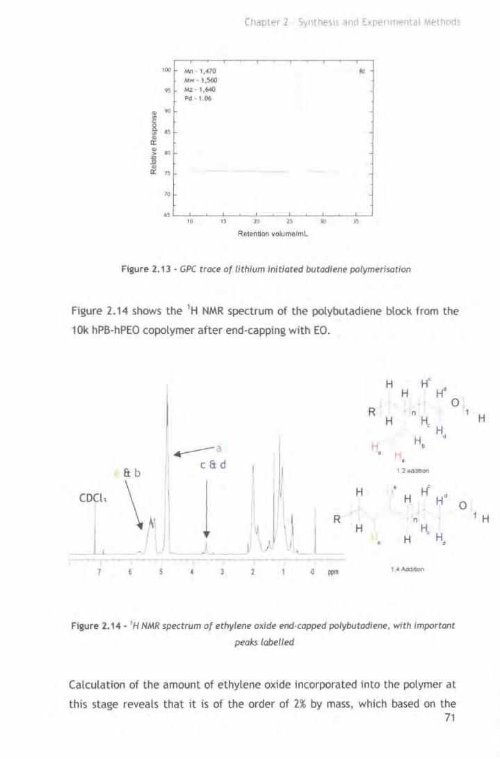
Chaoter 2 SyntheSIS and Expenmental Methods
100 fM. 1,470 RJ Mw ·1,560
95 Mz. 1,640 Pd · 1.06
Q) 90 tJ) c: 8. 85 tJ) Cl)
0::: Cl)
30 > ., (1)
a; 0::: 75
10
6~ 10 15 20 25 lO )5
Retention volume/mL
Figure 2.13 - GPC t race of lithium initiated butadiene polymerisation
Figure 2.14 shows the 1H NMR spectrum of the polybutadiene block from the
1 Ok hPB-hPEO copolymer after end-capping with EO.
CDCl1
& b
\~. 11 I I
.----c&d
\1
-i d '-- ~ l \}. -· ~--
rT TTrr~ --TTT-"-TT·...---
6 5 3 2
H H
R n H
H a
1 2 addltlon
H
H I
'..I.J R
1 4 Addrtlon
Figure 2.14- 1H NMR spectrum of ethylene oxide end-capped polybutadiene, with important
peaks labelled
Calculation of the amount of ethylene oxide incorporated into the polymer at
this stage reveals that it is of the order of 2% by mass, which based on the 71
1 H
1 H

Chapter 2 - Synthesis and Experimental Methods
molecular weight of the polymer being 1470 g mor1, gives a value of 30 g m:f1
for the molar mass of the ethylene oxide unit. Because the poly(butadiene) is
the dominant component, there are large errors in estimating the mass of
ethylene oxide incorporated, but this result does agree with the more rigorous
investigation of Quirk and Ma. 6
Figure 2.15 shows a GPC trace from the 5k hPB-hPEO copolymer, a single peak
only is observed.
Q)
Mn- 2,720 Mw- 3,100
80 Mz- 3,370 Pd -1.14
~ 60
8. :3 0:: 40 Q) >-= m a;
0:: 20
0
10 15 20 25 30 35
Retention volume/ml
Figure 2. 15 - GPC trace of Sk hPB-hPEO copolymer
Hence there was no excess potassium in solution. Had there been it would
have been highly likely that some homo poly(ethylene oxide) would also have
been forined which would have manifested itself on the GPC trace as either a
second peak, or a small shoulder on the main peak.
The 1H NMR spectra of the copolymers shows that the polymerisation of
ethylene oxide from the site of metallation on the end-capped chain has been
successful. 1H NMR spectroscopy was used to calculate the compositions of
the fully hydrogenous copolymers whilst 13C was used for the per-deuterated
variants. The compositions calculated from these are of the order expected
from the stoichiometry of the reaction, and is in contrast to that shown in
figure 2.14 for the end-capped poly(butadiene) chain. Figure 2.16 shows a
typical 1H NMR spectrum of the 10k hPB-hPEO copolymer.
72
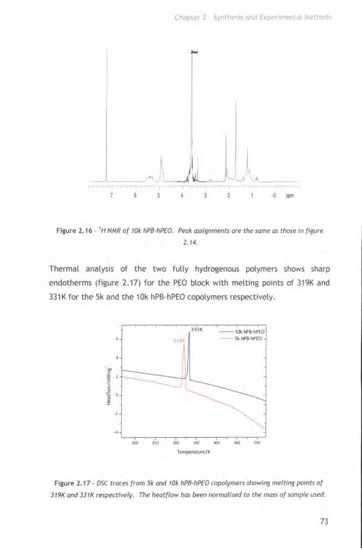
Chaptec 2 Synthests and Expenmental ,'llethod'i
r
I
___.._ __ rJ~l.~··."·-' t, '----7 6 5 4 3 2
Figure 2.16 - 1 H NMR of 101< hPB-hPEO. Peal< assignments are the same as those in figure
2.14.
Thermal analysis of the two fully hydrogenous polymers shows sharp
endotherms (figure 2.17) for the PEO block with melting points of 319K and
331K for the Sk and the 10k hPB-hPEO copolymers respectively.
6
200 250
331K
"
lOO
Temperature /K
--10k hPS..hPEO 5k hPS..hPEO
Figure 2.17 - DSC traces from 51< and 101< hPB-hPEO copolymers showing melting points of
319K and 331K respectively. The heatflow has been normalised to the mass of sample used.
73

Chapter 2 - Synthesis and Experimental Methods
2.6.2. Cross-linking reactions
Initial attempts to cross-link a micellar dispersion using this method of
McCarthy and eo-workers 19 proved successful. The reaction was attempted on
a relatively small scale, (ea. 0.2g polymer), and analysis of the end product by 1H NMR spectroscopy revealed there to be no olefinic protons present,
indicating a successful reaction. Interestingly, the polymer proved soluble in
water but not organic solvents making GPC analysis impossible. Attempts to
repeat the reaction on a larger scale were unsuccessful with copolymer being
recovered. Quite why this is the case remains unclear, although it is possible
that the procedure may not have been robust enough to be successfully scaled
up. Perhaps larger amounts of the initiators should have been used.
As with the previous method initial attempts to produce cross-linked micelles
using the method of Won, Davis and Bates9'
18 were successful, with the
product proving soluble in water, but not organic media. However, when the
reaction was scaled up to produce sufficient material for subsequent
investigations, the product recovered was cross-linked, but was only very
slightly soluble in water, and not at a level suitable for further studies. Again
the reason for this is unknown, but may become apparent with further
investigations.
Following the limited success of the previous method it was decided to
perform the reaction using the same basic procedure, but to use the solvent
which would be used in the SANS experiments to form the dispersion. This
way the reaction mixture could be diluted and used directly for the
experiments. As the SANS experiments required concentrations of up to 10%
it was decided to carry out the reaction at this concentration.
The reaction proved successful as demonstrated by the absence of olefinic
protons in the 1H NMR spectra, an example of which is shown in figure 2.18
along with that of the copolymer.
74

Chapter 2 - Synthesis and Experimental Methods
cross-linked micelles
-CHzCHzO-
/ 1 ,2 & 1 ,4 addition
\ 1 ,2 addition
/ copolymer
5.8 5.4 5.0 4.6 4.2 3.8 3
Figure 2.18- Olefinic region of 1H NMR spectra of copolymer and cross-linked micelles
showing the absence of the vinyl protons in the cross-linked species
The procedure was used to produce cross-linked micellar dispersions for all of
the contrast conditions utilised for the micellar dispersions, with the products
being used for subsequent SANS, SAXS, and light scattering experiments.
2.6.3. Light Scattering
2.6.3.1. Aqueous dispersions
Quasi-elastic light· scattering was used to determine the critical micelle
concentrations of the two fully hydrogenous copolymers in aqueous solution.
Figure 2.19 shows the graph obtained when plotting the average count rate
vs. log (cone) for 1 Ok hPB-hPEO.
75
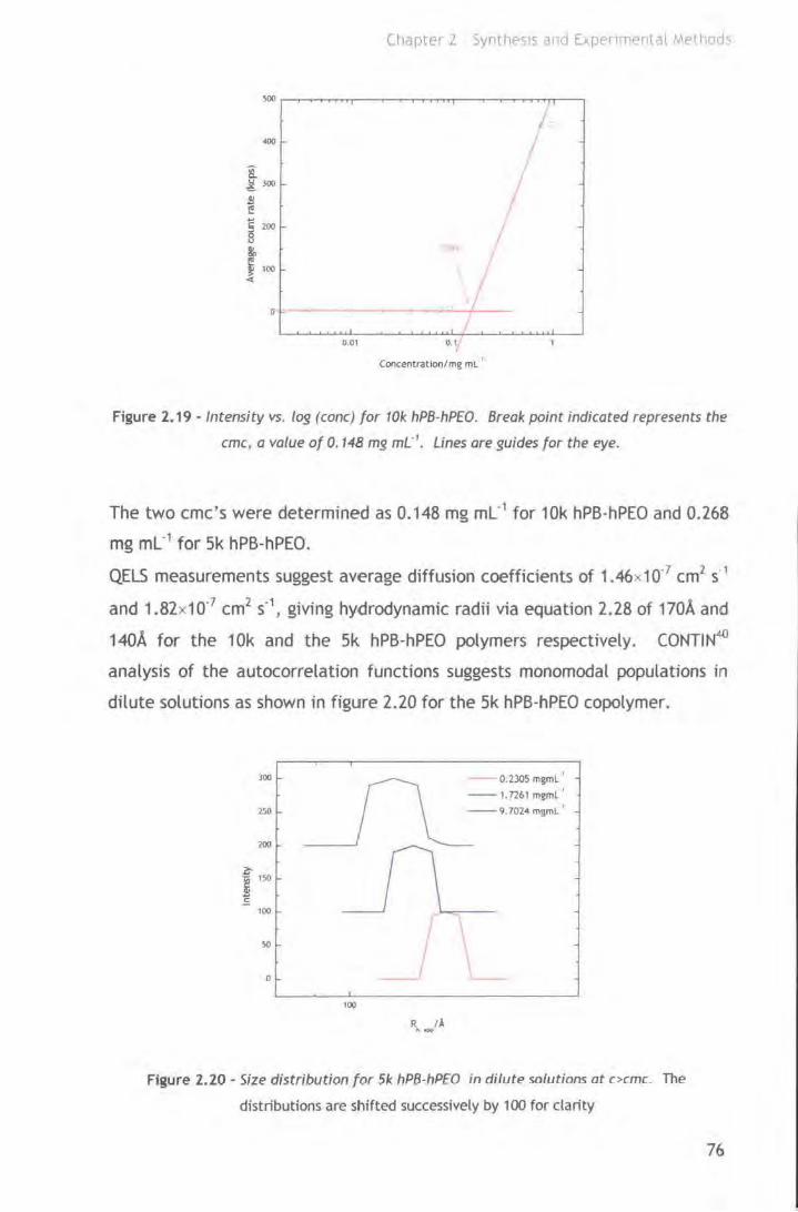
(l)apter 2 Svnt hes1s and Ex pet 1rnental Method c..
0
u 01 0. 1
Concentration/mg ml '
Figure 2.19 -Intensity vs. log (cone) for 101< hPB-hPEO. Break point indicated represents the
erne, a value of 0.148 mg mL" 1• Lines are guides for the eye.
The two erne's were determined as 0.148 mg ml·1 for 10k hPB-hPEO and 0.268
mg ml·1 for 5k hPB-hPEO.
QELS measurements suggest average diffusion coefficients of 1.46x10'7 cm2 s·1
and 1.82x10'7 cm2 s·1, giving hydrodynamic radii via equation 2.28 of 170A and
140A for the 10k and the Sk hPB-hPEO polymers respectively. CONTI~
analysis of the autocorrelation functions suggests monomodal populations in
dilute solutions as shown in figure 2.20 for the Sk hPB-hPEO copolymer.
300
250
200
100
0
100
0.23051111Jml '
-1.n61mgml'
-9.702<4 mjlml '
Figure 2.20- Size distribution for 51< hPB-hPEO in dilute solutions at c>cmc. The
distributions are shifted successively by 100 for clarity
76

Chapter 2 Svnthes1s ::~nd Expenmental Methoci-:
SLS data proved inconclusive, with the molecular weights, and radli of
gyration determined not matching what could be reasonably expected. Both
Zimm and Debye methods34 were applied to the hPB-hPEO copolymers for
both molecular weights, with figure 2.21 showing a Zimm plot for the 1 Ok
hPB-hPEO copolymer.
) .0x10
on -g 2.0x10 .... cC ._ ::i
1 Ol\10
Expenmental data • Extrapolated data
0.0 .___.___. _ _.__-..l.._....____.__.. _ _._____._ _ _._____, 0.0 0.2 0.~ 0.6 0.8 1.0
sin' (e /2) •100c-cmc/mgml '
Figure 2.21 - Zimm plot for 10k hPB-hP£0 in water generated using equation 2.23. Vertical
lines are fits through concentration series at a given angle and the horizontal lines are fits
through angular series at a given concentration.
The erne determination and QELS data are dealt with in sections 3.2 and 3.3,
and the SLS in section 3.4.
2.6.3.2. Cross-linked micelles
QELS and SLS experiments were performed on the cross-linked micelles and
comparisons made between them and the "virgin" micelles.
QELS experiments revealed that the micelle dimensions were smaller
following cross-linking with the 1 Ok micelles having a hydrodynamic radius of
156A and the 5k 94A. The size distributions were still monomodal in dilute
solution, although they had increased in width (figure 1.22).
77

Cl'apter '2 Synthests a.,d Expenment al Method.,
)()()
o. 348 rnsmL'' -- 1.84 mgml 1
250 -9.804rnsmt '
200
?;-
i c
150
100
50
0
100
I\ ... lA
Figure 2.22 - Size distribution for 10k hPB-hP£0 in dilute solutions. The distributions are
shifted successively by 100 for clarity.
SLS data proved as troublesome as for the virgin micelles, with the data not
being reliable.
The QELS studies of cross-linked micelles are discussed in section 4.3, with
the SLS studies in section 4.4.
2.6.4. Small-angle X-ray scattering
2.6.4.1. Aqueous dispersions
Typical examples of the data collected are presented in figures 2.23 and 2.24
for the 5k and 1 Ok hPB-hPEO respectively, but discussion and treatment of
these and other data are left until later chapters.
78
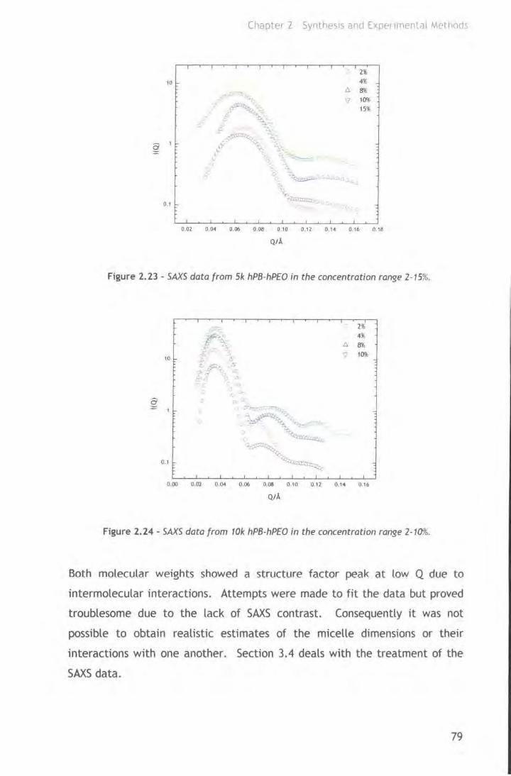
Chapter 2 Synthes1s and £xpenrnental Methods
10
g 1
0.1
0.02 0.().4 0.06 0.08 0.10 0.11 O.H 0.16 0. 15
Qtl
Figure 2.23- SAXS data from 5k hPB-hPEO in the concentration range 2- 15%.
10
0.1
o.oo 0.02 o.o.c o06 o.oa 0.10 0.12 o.,. 0.16
QtA.
Figure 2.24 - SAXS data from 10k hPB-hPEO in the concentration range 2-10%.
Both molecular weights showed a structure factor peak at low Q due to
intermolecular interactions. Attempts were made to fit the data but proved
troublesome due to the lack of SAXS contrast. Consequently it was not
possible to obtain realistic estimates of the micelle dimensions or their
interactions with one another. Section 3.4 deals with the treatment of the
SAXS data.
79
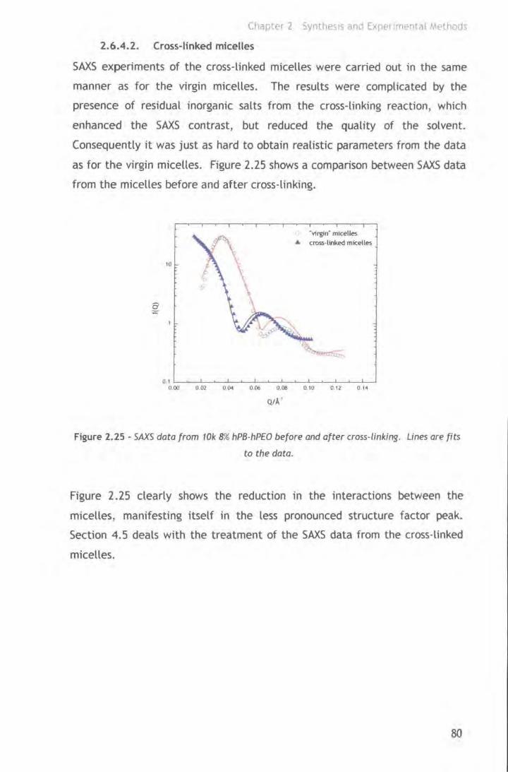
Chapter 2 Synthes1s and E><perJrnental Methods
2.6.4.2. Cross-linked micelles
SAXS experiments of the cross-linked micelles were carried out in the same
manner as for the virgin micelles. The results were complicated by the
presence of residual inorganic salts from the cross-linking reaction, which
enhanced the SAXS contrast, but reduced the quality of the solvent.
Consequently it was just as hard to obtain realistic parameters from the data
as for the virgin micelles. Figure 2.25 shows a comparison between SAXS data
from the micelles before and after cross-linking.
·virgin· micelles A cross-linked mlc:eUes
10
0 . I L...-..__.l--...__..L.-_.__...l..-_.__...,~.__.___..!.__._-l....._..__,~__,
0 00 0.01 0 04 0.06 0.08 0.10 0. 12 0.1.
Q!J.. '
Figure 2.25- SAXS data f rom 10k 8% hPB-hP£0 before and af ter cross-linking. Lines are fits
to the data.
Figure 2.25 clearly shows the reduction in the interactions between the
micelles,. manifesting itself in the less pronounced structure factor peak.
Section 4.5 deals with the treatment of the SAXS data from the cross-linked
micelles.
80

Chapter 2 SyntheSlS and Expenmental Methods
2.6.5. Small-Angle Neutron scattering
2.6.5.1. Aqueous dispersions
Data providing an overview of that collected is presented here. As with the
data from the previous sections it will be discussed in more detail later.
Figures 2.26 and 2.27 show the scattering from 1% and 10% dispersions of all
three contrasts for the 10k and 5k series respectively.
100
'1\. 10 \ .. .,. "'g a ~
0.1
le! 0.01
1E· l
0.00 0.05 0.10 015
Q/A '
hPB·hPEO hPB-<lPEO
0 dP6-hPEO
0 20 0~
Figure 2.26- SANS data from 1% dispersions of 10k series
100 hPB-hPEO
~ hPB-<lPEO
0 dPB-hPEO 10
' 'lll E ~ a :g 0.1 .... ta
0.01
1E·l
0.00 0.05 0.10 0. 15 0 ]0 015
QIA·'
Figure 2. 27 - SANS data from 10% dispersions of 5k series
81

Chapter 2 - Synthesis and Experimental Methods
Figures 2.26 and 2.27 clearly show the differences in the scattering due to the
effects of both concentration and contrast. The 10% dispersions show a
pronounced structure factor peak at low Q due to intermicellar interactions,
whilst this is distinctly absent in the 1% dispersions suggesting the
concentration is sufficiently dilute that the micelles do not exhibit a high
degree of long-range order. The scattering from the dispersions where the
corona is contrast matched (i.e. scattering from the core only) is considerably
weaker than for the other two contrasts as one would expect given that the
core-forming block is the minority component of the copolymers.
From fits to the data it was possible to determine the micelle dimensions and
association numbers, with the Sk micelles having core radii of ea 20A and a
shell thickness of between 60 and 1 OOA, whilst the 1 Ok micelles had core radii
of 40A and a corona thickness of ea 115A. The two molecular weights
exhibited contrasting association behaviour with the Sk micelles having only
moderate association numbers of 30-40 whilst the 1 Ok micelles had high
association numbers of 100-200. The treatment of the dilute micellar
dispersion is dealt with in section 3.5.2, whilst the more concentrated
dispersions with greater organisation are tackled in section 3.5.3
2.6.5.2. Cross-linked micelles
The cross-linked micelles were investigated by SANS over the same
concentration range as for the virgin micelles. Figure 2.28 demonstrates the
differences in the data between the micelles before and after cross-linking,
with scattering from a 1% dispersion of the Sk hPB-hPEO micelles shown.
82
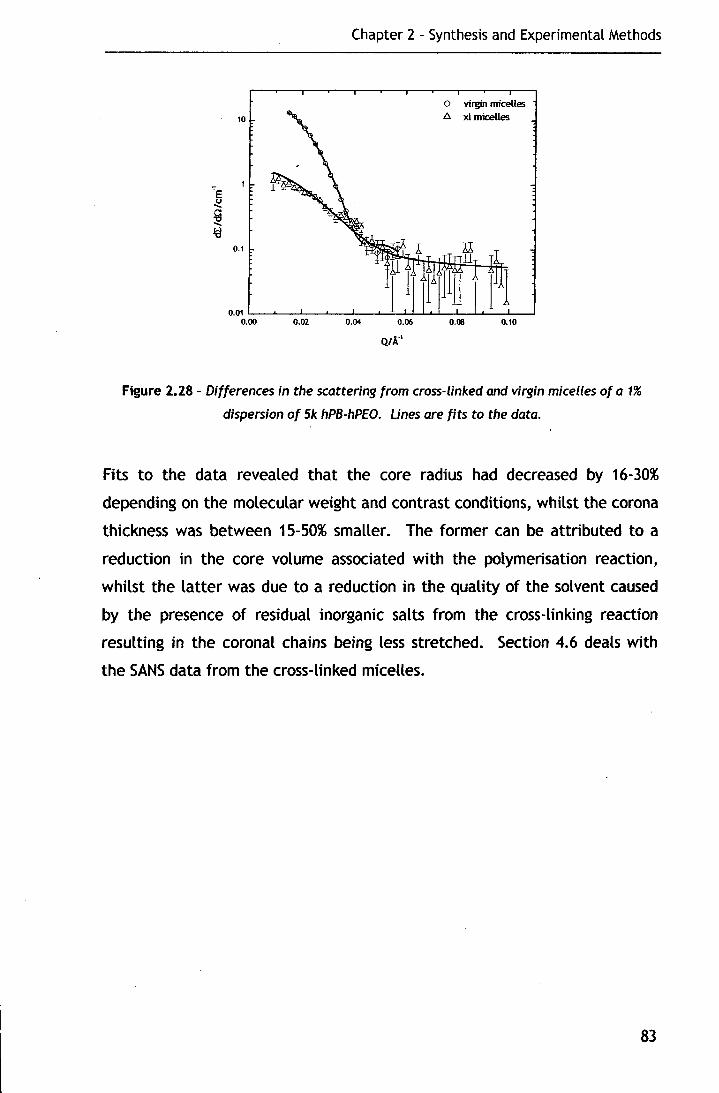
10
0.1
0.02
Chapter 2 - Synthesis and Experimental Methods
0.04 0.06
Qtl>:'
o virgin micelles t:. xl micelles
0.08 0.10
Figure 2.28 - Differences in the scattering from cross-linked and virgin micelles of a 1%
dispersion of 5k hPB-hPEO. Unes are fits to the data.
Fits to the data revealed that the core radius had decreased by 16-30%
depending on the molecular weight and contrast conditions, whilst the corona
thickness was between 15-50% smaller. The former can be attributed to a
reduction in the core volume associated with the polymerisation reaction,
whilst the latter was due to a reduction in the quality of the solvent caused
by the presence of residual inorganic salts from the cross-linking reaction
resulting in the coronal chains being less stretched. Section 4.6 deals with
the SANS data from the cross-linked micelles.
83

Chapter 2 - Synthesis and Experimental Methods
2.7. Glossary of symbols
The symbols used in the body of the text and the equations are defined here
in the order in which they appear in the text.
2. 7.1. Small-angle scattering
Mw - weight average molecular weight
Az - second virial coefficient
Rg- radius of gyration
p - micelle association number
erne - critical micelle concentration
cmt - critical micelle temperature
Dt - translational diffusion coefficient
Dr - rotational diffusion coefficient
Rh- hydrodynamic radius
A. - radiation wavelength
ki- incident wave vector
ks- scattered wave vector
e- scattering angle
Q - scattering vector
d- domain size
I(Q) - scattering intensity
lo- Incident flux
L\Q - solid angle element defined by the size of a detector pixel
11 - detector efficiency
T - neutron transmission of sample
Vs - volume of sample illuminated by neutron beam
awn -differential scattering cross-section
N- number concentration of scattering centres
V P - volume of one scattering centre
(t::\p)2- contrast factor
P(Q)- particle form factor
S(Q) - particle structure factor
B - background
p- X-ray/neutron scattering length density
84
Chapter 2 - Synthesis and Experimental Methods
& - bulk ,density
NA - Avogadro's number
M - molar mass
~- X-ray/neutron scattering length
R- sphere radius
Pc - core scattering length density
Ps- shell scattering length density
Pm- solvent scattering length density
Re - core radius
Res - micelle radius
r - separation distance
Rtis- hard sphere radius
h - hard sphere volume faction
2. 7. 2. Static light scattering
lo - intensity of scattered light at angle e lo- incident intensity
no- solvent refractive index
r - distance between scattering molecule and detector
A.o - incident wavelength radiation
NA - Avogadro's number
d'lcic- specific refractive index increment
M - molar mass
c- concentration
A2 - second virial coefficient
Re - Rayleigh ratio at angle e K - optical constant
· Rg- radius of gyration
k- plotting constant
85

Chapter 2 - Synthesis and Experimental Methods
2. 7. 3. Quasi-elastic light scattering
g(t) - intensity autocorrelation function
l(t) - intensity at time t
l(t+-r)- intensity at time t+-r
-r - delay time
r - relaxation rate
Q- scattering vector
D - diffusion coefficient
ks- Boltzmann's constant
T- temperature
11 - sol vent viscosity
RtJ - hydrodynamic radius
K - cumulant coefficient
2.8. .Bibliography
2
3
4
5
6
7
8
9
10
11
12
13
M. Szwarc, Nature, 1956, 178, 1168.
H. L. Hsieh and R. P. Quirk, 'Anionic Polymerisation: Principles and
Practical Applications', Marcel Dekker, New York, 1996.
S. Bywater, Y. Firat, and P. E. Black, J Polym Sci, A, Polym Chem.,
1984, 22, 669.
R. Milner and R. N. Young, Polymer, 1982, 23, 1636.
J. Brandup and E. H. lmmergut, 'Polymer Handbook', 3rd, ed., John
Wiley and Sons, Toronto, 1989.
R. P. Quirk and J. J. Ma, J. Polym. Sci. A, Polym. Chem., 1988, 26,
2031.
S. Forster and E. Kramer, Macromolecules, 1999, 32, 2783.
M. A. Hillmyer and F. S. Bates, Macromolecules, 1996, 29, 6994.
Y. Y. Won, H. T. Davis, and F. S. Bates, Science, 1999, 283, 960.
P. Hoerner, et al., Macromol. Chem. Phys., 1998, 199, 343.
S. Forster and M. Antonietti, Adv. Mater., 1998, 10, 195.
J. Bowers, et al., Langmuir, 2001, 17, 131.
G. L. Jialanella, E. M. Firer, and I. Piirma, J Polym Sci, A, Polym
Chem., 1992, 30, 1925.
86
14
15
16
17
18
19
20
21
22
23
24
25
26
27
28
29
30
31
32
33
34
Chapter 2 - Synthesis and Experimental Methods
M. Muthukumar, C. K. Ober, and E. L. Thomas, Science, 1997, 277,
1225.
Z. Tuzar, et al., Macromol. Chem. Phys., 1982, 183, 399.
D. J. Wilson and~. Reiss, Eur. Polym. J., 1988, 24, 617.
G. Odian, 'Principles of Polymerisation', 3rd, ed., John Wiley & Sons
Inc., New York, 1991.
Y. Y. Won, et al., J. Phys. Chem. 8, 2001, 105, 8302.
T. F. McCarthy, et al., J. App. Polym. Sci., 1998, 70, 2211.
S. M. King, in 'Modern Techniques of Polymer Characterisation', ed. R.
A. Pethrick and J. V. Dawkins, John Wiley & Sons, London, 1999.
C. E. Williams, R. P. May, and A. Guinier, in 'X-ray Characterisation of
Materials', ed. E. lifshin, Wiley-VCH, Weinheim, 1999.
B. Chu and Z. Zhou, in 'Nonionic surfactants: Polyoxyalkylene block
copolymers', ed. V. M. Nace, Marcel Dekker, New York, 1996.
R. W. Richards, in 'Comprehensive Polymer Science', ed. C. Booth and
C. Price, Pergamon, Oxford, 1989.
L. A. Feigin and D. I. Svergum, 'Structure Analysis by Small-angle X-ray
and Neutron Scattering', Plenum Press, New York, 1987.
'Small Angle X-ray Scattering', ed. 0. Glatter and 0. Kratky, Academic
Press, 1982.
R. H. Ottewill, in 'Colloidal Dispersions', ed. J. W. Goodwin, Royal
Society of Chemistry, London, 1982.
J. S. Pedersen, Adv. Colloid Interface Sci., 1997, 70, 171.
L. Rayleigh, Proc. Roy. Soc. London, Ser. A., 1911, 84, 25.
G. J. Bown, R. W. Richards, and R. K. Heenan, Polymer, 2001, 42,
7663.
J. K. Perkus and G. J. Yevick, Phys. Rev, 1958, 110, 1.
N. W. Ashcroft and J. Lekner, Phys. Rev, 1966, 145, 83.
R. H. Ottewill, in 'Colloidal Dispersions', ed. J. W. Goodwin, Royal
Society of Chemistry, London, 1982.
P. N. Pusey, in 'Colloidal Dispersions', ed. J. W. Goodwin, Royal Society
of Chemistry, London, 1982.
P. Kratochvil, 'Classical light Scattering From Polymer Solutions', A. D.
Jenkins, Elsevier, New York, 1987.
87
35
36
37
38
39
40
41
42
43
Chapter 2 Synthec;1s ~~~cl Expenmentat Method
R. B. Filippen, in 'Modern Methods of Polymer Characterisation·, ed. H.
G. Barth and J. W. Mays, Wiley and Sons, New York, 1991.
I. A. Katime and J. R. Quintana, in 'Comprehensive Polymer Science',
ed. C. Booth and C. Price, Pergamon, Oxford, 1989.
W. Burchard, in 'Applied Fibre Science·, ed. F. Happey, Academic Press,
1978.
G. D. Phillies, J. Appl. Polym. Sci: Appl. Polym. Symp. , 1989, 43 , 275.
D. E. Koppel, J. Chem. Phys. , 1972, 57, 4814.
S. W. Provencher, Makromol. Chem., 1979, 180, 201.
0. Glatter and K. Gruber, J. Appl. Cryst., 1993, 26, 512.
http://www. is is. rl.ac. uk/largescale /log
R. K. Heenan and 5. M. King, The LoQ Handbook', RAL-TR-96-036,
Rutherford Appleton Laboratory, Didcot, 1996.
88
Chapter 3 - Block Copolymer Micelles
3. Block Copolymer
Micelles
89

Chapter 3 - Block Copolymer Micelles
3. 1. Introduction
Poly(butadiene)-Poly(ethylene oxide) (PB-PEO) block copolymers synthesised
by the route described in chapter two are amphiphilic, and as a qmsequence
form micelles when dispersed in water, which is a selective solvent for the
poly(ethylene oxide) block. Micelle formation is generally only observed
above the critical micelle concentration (erne), which can be defined as the
concentration at which micelle formation becomes sufficiently appreciable to
be detected by a given experimental technique. 1
A considerable amount of research has been invested in the study of the
structure, organisation and properties of amphiphilic block copolymers in
aqueous solutions over the past decade. 2"7 The key results of this work were
presented in chapter one, with particular emphasis on the work of Bates and
eo-workers into the study of PB-PEO in aqueous solution. A comparison of this
work with new results presented herein will now be discussed; a perspective
of these new results compared to those for different amphiphilic block
copolymers will also be presented.
3~2.1. How do we study block copolymer micelles?
Chapter two discussed the basic theory underpinning radiation scattering
techniques that have formed the backbone of this research. The information
obtainable from each technique was also presented, but will be briefly
reviewed here for clarity.
The structural detail that can be resolved from a particular technique is
inversely proportional to the magnitude of the scattering vector, which is
given by equation 3.1
JQJ = Q = 4nn sin(B/2) A.
Equation 3.1
Thus static light scattering, whose Q values range from ea. 5x1 o·3 to 5x1 o·2
nm·1 yields information on the radius of gyration but not the internal
structure. Conversely, SAXS and SANS with Q values of 3x10"3 to 5 nm·1 allows
90

Chapter 3 - Block Copolymer Micelles
intramicellar structure to be elucidated. Table 3.1 details the information
that each of the techniques can yield.
SLS QELS SAXS SANS
Q values/nm·1 -5x1o·J_
-5x10"3-5x10.2 5x10.3-5 5x10"2
Information Rg, Mw, D, Rh, size Rg, internal structure, micelle
obtainable Az, p distribution shape, structure and ordering
Table 3.1 - Q values and information yielded from scattering techniques. Rg is the radius of
gyration, Mw is the weight average molecular weight, A2 is the second virial coefficient, D is
the diffusion coefficient, Rh is the hydrodynamic radius.
The techniques are complementary to one another, and in order to obtain the
maximum amount of information for the micelles a combination of the four
should be employed, as used here. The results obtained from each of the
techniques will be presented and discussed individually, with the final part of
this chapter drawing all of the results together.
3.2. Quasi-Elastic Light Scattering
QELS is a powerful, widely used tool for the study of block copolymer
micelles. 8"11 As discussed earlier in section 2.4.2.2, QELS yields an intensity
autocorrelation function, which when suitably analysed provides invaluable
information about the. hydrodynamic behaviour of micelles. As the intensity is
sensitive to low mass concentrations of micelles it provides a convenient
method for demonstrating their presence in aqueous solution. 3• 12
Using the method of CONTIN13 analysis discussed in section 2.4.2.2 the
intensity distribution of the apparent translational diffusion coefficient can be
obtained, and by applying the Stokes-Einstein equation (equation 2.28), viz
Dapp = kBT the apparent diffusion coefficient can be converted to the 6;rqRh,app
corresponding distribution of apparent hydrodynamic radii, Rh, app·
91
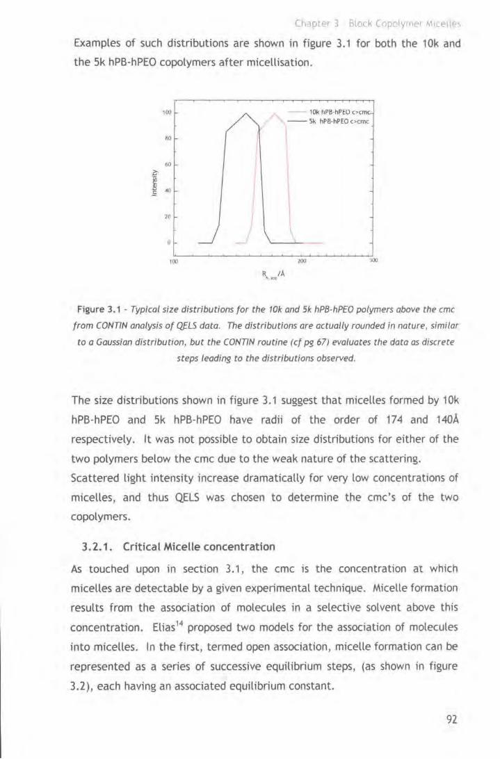
Ch:~pte>r 1 Block Copol.yrn("f Micelles
Examples of such distributions are shown in figure 3.1 for both the 10k and
the Sk hPB-hPEO copolymers after micellisation.
;:;-
~ E
tOO
HO
bO
4()
20
0
100
IOk hPB-hPEO c>cm
-- 511 hPB-hPEO c>cmc
Figure 3.1 - Typical size distributions for the 10k and 5k hPB-hP£0 polymers above the erne
from CONTIN analysis of QELS data. The distributions are actually rounded in nature, similar
to a Gaussian distribution, but the CONTIN routine (cf pg 67) evaluates the data as discrete
steps leading to the distributions observed.
The size distributions shown in figure 3.1 suggest that micelles formed by 1 Ok
hPB-hPEO and Sk hPB-hPEO have radii of the order of 174 and 140A
respectively. lt was not possible to obtain size distributions for either of the
two polymers below the erne due to the weak nature of the scattering.
Scattered light intensity increase dramatically for very low concentrations of
micelles, and thus QELS was chosen to determine the erne's of the two
copolymers.
3.2.1 . Critical Micelle concentration
As touched upon in section 3.1, the erne is the concentration at which
micelles are detectable by a given experimental technique. Micelle formation
results from the association of molecules in a selective solvent above this
concentration. Elias 14 proposed two models for the association of molecules
into micelles. In the first, termed open association, micelle formation can be
represented as a series of successive equilibrium steps, (as shown in figure
3.2), each having an associated equilibrium constant.
92

Chapter 3 - Block Copolymer Micelles
A1 + A1 k2
~
~+ A1 k3
~
A3 + A1 k4
A4
~-1+ A1 kN
AN
Figure 3.2- Open association
If the different association steps are equivalent, then one association
constant, ko that is given by equation 3.2, can define the system.
Equation 3.2
This model leads to a broad continuous distribution of micelle sizes, and is
similar to the equilibrium in condensation polymerisation in terms of the size
distribution. However it does not lead to a definable erne.
The second model, termed closed association, can be represented by an
equilibrium between micelles of association number p, and unimers, as shown
in figure 3.3.
Figure 3.3- Closed association
The association constant, kc is given by equation 3.3.
Equation 3.3
This model gives rise to a narrow distribution of micelle sizes and can be
compared to the monomer /polymer equilibrium in addition polymerisation. lt
also allows for the concept of a erne.
Block copolymers undergoing micellisation exhibit a erne, and show a narrow
distribution of particle sizes, suggesting the closed association model is the
most appropriate. 15
93
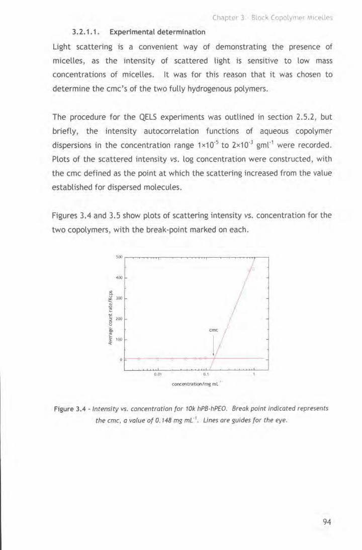
Chapter 3 Block Copolvmer Mlct-llc>c.;
3.2.1.1. Experimental determination
Light scattering is a convenient way of demonstrating the presence of
micelles, as the intensity of scattered light is sensitive to low mass
concentrations of micelles. lt was for this reason that it was chosen to
determine the erne's of the two fully hydrogenous polymers.
The procedure for the QELS experiments was outlined in section 2.5.2, but
briefly, the intensity autocorrelation functions of aqueous copolymer
dispersions in the concentration range 1 x1 o·5 to 2x10·3 gmr1 were recorded.
Plots of the scattered intensity vs. log concentration were constructed, with
the erne defined as the point at which the scattering increased from the value
established for dispersed molecules.
Figures 3.4 and 3.5 show plots of scattering intensity vs. concentration for the
two copolymers, with the break-point marked on each.
100
0
cmc
I; 0.1
concentrataon/mg ml '
Figure 3.4 - Intensity vs. concentration for 10k hPB-hP£0. Break point indicated represents
the cmc, a value of 0.148 mg mL''. Lines are guides for the eye.
94
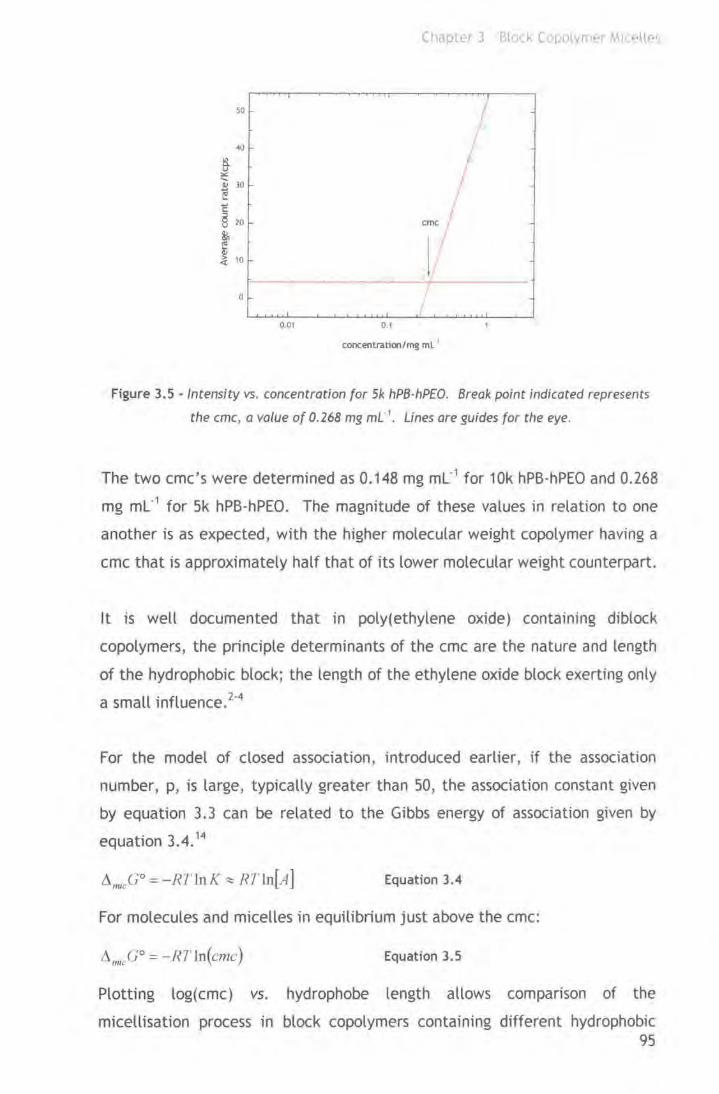
50
.w IS. u ::.:: ...... .!! 30 !! c § 20
~ f ~ 10
0
0.01
Chapt~r 3 Block Copolvrnt'r MrceHe~
erne
0.1
concentratlon/mg mL '
Figure 3.5 ·Intensity vs. concentration for Sk hPB·hPEO. Break point indicated represents
the erne, a value of 0.268 mg mL '. Lines are guides for the eye.
The two erne's were determined as 0.148 mg ml·1 for 10k hPB-hPEO and 0.268
mg mL·1 for 5k hPB-hPEO. The magnitude of these values in relation to one
another is as expected, with the higher molecular weight copolymer having a
erne that is approximately half that of its lower molecular weight counterpart.
It is well documented that in poly(ethylene oxide) containing diblock
copolymers, the principle determinants of the erne are the nature and length
of the hydrophobic block; the length of the ethylene oxide block exerting only
a small influence. 2.4
For the model of closed association, introduced earlier, if the association
number, p, is large, typically greater than 50, the association constant given
by equation 3.3 can be related to the Gibbs energy of association given by
equation 3.4. 14
Equation 3.4
For molecules and micelles in equilibrium just above the erne:
C!.,1c(J 0 = -RJ' Jn(cmc) Equation 3.5
Plotting log(cmc) vs. hydrophobe length allows comparison of the
micellisation process in block copolymers containing different hydrophobic 95
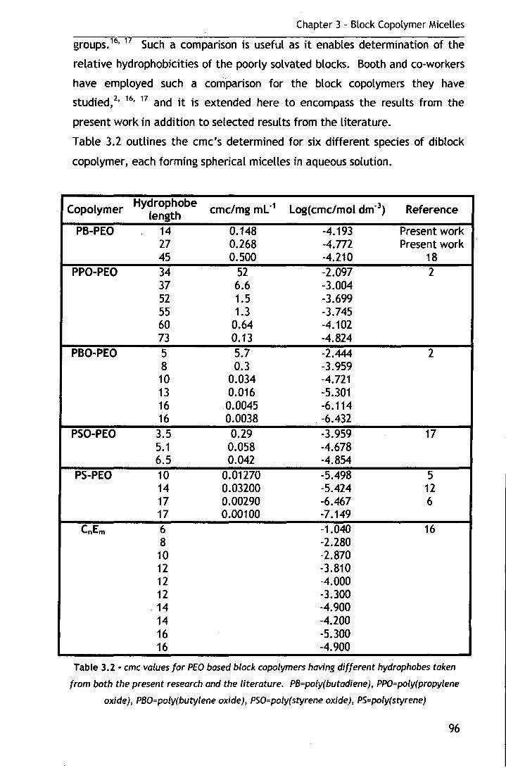
Chapter 3 - Block Copolymer Micelles
groups. 16'
17 Such a comparison is useful as it enables determination of the
relative hydrophobicities of the poorly solvated blocks. Booth and eo-workers
have employed such a coni.parison for the block copolymers they have
studied/' 16'
17 and it is extended here to encompass the results from the
present work in addition to selected results from the literature.
Table 3.2 outlines the erne's determined for six different species of diblock
copolymer, each forming spherical micelles in aqueous solution.
Copolymer Hydrophobe cmc/mg ml-1 Log(cmc/mol dm"3
) Reference length PB-PEO 14 0.148 -4.193 Present work
27 0.268 -4.n2 Present work 45 0.500 -4.210 18
PPO-PEO 34 52 -2.097 2 37 6.6 -3.004 52 1.5 -3.699 55 1.3 -3.745 60 0.64 -4.102 73 0.13 -4.824
PBO-PEO 5 5.7 -2.444 2 8 0.3 -3.959 10 0.034 -4.721 13 0.016 -5.301 16 0.0045 -6.114 16 0.0038 . -6.432
PSO-PEO 3.5 0.29 -3.959 17 5.1 0.058 -4.678 6.5 0.042 -4.854
PS-PEO 10 0.01270 -5.498 5 14 0.03200 -5.424 12 17 0.00290 -6.467 6 17 0.00100 -7.149
CnEm 6 -1.040 16 8 -2.280 10 -2.870 12 -3.810 12 -4.000 12 -3.300 14 -4.900 14 -4.200 16 -5.300 16 -4.900
Table 3.2- erne values for PEO based block copolymers having different hydrophobes taken
from both the present research and the literature. PB=poly(butadiene), PPO=poly(propylene
oxide), PBO=poly(butylene oxide), PSO=poly(styrene oxide), PS=poly(styrene)
96

Chapter 3 Glot:k Copolvmt r M! dlL's
Figure 3.6 shows a plot of log(cmc) vs. hydrophobe length, n, constructed
using the data from table 3.2.
·0.~ ,--.-.,.--.--,----r--T""""",---,.---.-~-.--..-....--,--,
., (I
I 5
·2 0
·2.~
~- ·3.0
~ · l 5
-g ·4.0
~ ·<1.5
~ -5.0
:9 -5.5
-6 0
~ \
' 10 20
PPO·PE PBO-PEO PSO-PEO PS-PEO
• PB·PEO 1l' c.E.
G
30 40 50 60 70 1!0
hydrophobe block length (n)
Figure 3.6 - Plot of log(cmc) vs hydrophobe length for PEO based block copolymers with
different hydrophobes, abbreviations are as in table 3.2. The circled point is that due to
Zheng and Davis.
One of the most striking features of figure 3.6 is the difference in the slope
for the PB-PEO copolymers when compared to the other species, with it being
significantly shallower. The line through the PB-PEO points was calculated
using only the results from the present research, as there was some question
mark over the validity of the result produced by Zheng and Davis18 (that
circled in figure 3.6 ). The result used originates from graphical interpretation
of their data rather than the result quoted in the text of the paper, with the
two values being vastly different, the latter quoted as 1.1 x1 o·4g L·1•
Using the chain length required to attain a given erne value as an indicator,
the relative hydophobicities can be calculated from the linear relationships
determined in figure 3.6. Such a comparison yields relative hydrophobicities
in the ration of 1:3:5:6:11:13 for PPO:PB:Cn:PBO:PS:PSO respectively.
Davies and Rideal proposed a system to calculate a hydrophile-lipophile
balance (HLB) based upon the functional groups present in the molecule. 19•
20
This can be used as an indication of the hydrophobic nature of a molecule by
the score given from equation 3.6
97
Chapter 3 - Block Copolymer Micelles
HLB =·"f) hydrophilic group numbers)- "):)hydrophobic group numbers)+ 7 Equation 3.6
The lower the total score, the more hydrophobic a molecule is. Lipophilic
groups such as CH2 units are given a group number of 0.475, whilst PEO has a
group number of 0.33. Charged species have higher group numbers still.
Calculation of HLB numbers for PPO-PEO, PBO-PEO and PB-PEO give values of
5. 905, 5.43 and 5.43 respectively, indicating that PB and PBO have similar
hydrophobic character, and are more hydrophobic that PPO. This can only be
taken as an indicative value and not an absolute one.
For some polymer blocks in the list given the data set available is very small,
therefore the ratio of hydophobicities given should be taken as indicative
rather than quantitative.
3.2.2. Average Hydrodynamic radii
The concentration dependence of the apparent average diffusion coefficient
(Dapp) determined from analysis of the intensity autocorrelation function can
be related to the translational diffusion coefficient of the micelles at zero
concentration by equation 3.78'
21"23
Equation 3. 7
kcJ is the diffusion second virial coefficient, which can be related to the
thermodynamic second virial coefficient by equation 3.88'
23
Equation 3.8
kt is the frictional coefficient and v is the partial specific volume of micelles
in solution.
Figure 3.7 shows plots of Dapp vs. (c-cmc) for polymers 10k hPB-hPEO and 5k
hPB-hPEO in aqueous solution.
98
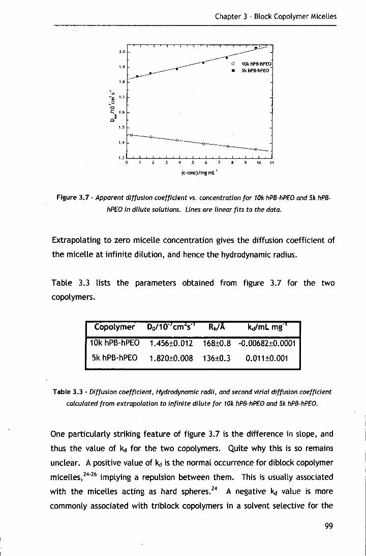
Chapter 3 - Block Copolymer Micelles
2.0 •.,.:...---___________
__________.. o 10k hPB-hPEO
--------· • Sk hPB-hPEO
--------1.9
1.8
., Ill
NE 1.7 ~u 0 ::::: 1.6
0~ 1.5
1.4~
3 4 5 6 7 8
(c-cmc)/mg ml''
-10 11
Figure 3. 7 - Apparent diffusion coefficient vs. concentration for 10k hPB-hPEO and Sk hPB
hPEO in dilute solutions. Lines are linear fits to the data.
Extrapolating to zero micelle concentration gives the diffusion coefficient of
the micelle at infinite dilution, and hence the hydrodynamic radius.
Table 3.3 lists the parameters obtained from figure 3.7 for the two
copolymers.
10k hPB-hPEO 1.456±0.012 168±0.8 -0.00682±0.0001
Sk hPB-hPEO 1.820±0.008 136±0.3 0.011±0.001
Table 3.3 -Diffusion coefficient, Hydrodynamic radii, and second virial diffusion coefficient
calculated from extrapolation to infinite dilute for 10k hPB-hPEO and Sk hPB-hPEO.
One particularly striking feature of figure 3.7 is the difference in slope, and
thus the value of kct for the two copolymers. Quite why this is so remains
unclear. A positive value of kct is the normal occurrence for diblock copolymer
micelles, 24.26 implying a repulsion between them. This is usually associated
with the micelles acting as hard spheres. 24 A negative kct value is more
commonly associated with triblock copolymers in a solvent selective for the
99

Chapter 3 - Block Copolymer Micelles
middle block. 21• u:-ia Under these conditions flower-like micelles are formed
with some of the end blocks dangling in solution leading to attractive
interactions. The synthetic procedure employed precludes the formation of
such copolymers and so the negative value must be due to some other factor.
Table 3.4 details hydrodynamic radii of poly(ethylene oxide) based diblock
copolymers of comparable molecular characteristics to those studied here.
Chapter one introduced the scaling approaches applied to micelles by
Halperin29 and others. These are discussed in more detail in section 3.5.2.3,
but briefly, the values of the micelle radius, R, can be estimated from the
degree of polymerisation of both blocks and the segment length using
equation 3. 9
Equation 3. 9
where Ne is the degree of polymerisation of the core block, NA is the degree of
polymerisation of the shell block, and a is the segment length.
The model assumes the segment length to be equal for both blocks, which
although not strictly correct, the errors associated with such an assumption
are sufficiently small as to allow it to be used. The segment length can be
determined by the cube root of the volume of one repeat unit, which
Nagarajan and Ganesh30 reported as 64.6A for ethylene oxide, giving a
segment length of 4.01A. The values expected from this relationship are also
given in table 3.4 for the copolymers listed, using the segment length of
ethylene oxide in all of the calculations.
Strictly speaking, the degree of polymerisation of the two blocks in the
copolymers should be normalised with respect to the melt densities of each
block, using equation 3.10.
Equation 3.10
where rv is the normalised degree of polymerisation, NA and Ne are the
respective degrees of polymerisation of each block, MA and Me are the
molecular weights of each block, and PA and pe are the melt densities of each
block. This correction was not applied here, but in any future efforts to fit
100

Chapter 3 - Block Copolymer Micelles
similar: data should be applied. This changes the molecular volumes by ea
15%.
Wt% Mw Rh/A RIA Copolymer ~:R Reference
EO copolymer
B14Es9 81 4100 135 92.4 1.46 Present work
Bz1E164 83 8800 168 146.6 1.15 Present work
~3609 74 2620 69 54.5 1.27 31
E.wB01o 71 2580 73 53.0 1.38
E9oB01o 85 4820 95 86.3 1.10
E96B01s n 5690 155 98.5 1.57
E184B01s 86 9670 195 145.6 1.34
E106B016 80 5990 73 102.6 0.71 24
E216B016 89 10700 200 157.3 1.27
EsoS03.5 84 2670 66 51.3 1.29 17
EsoSOs.1 78 2920 69 54.4 1.27
Es1S06.s 74 3110 72 57.3 1.26
s16E1ss 80 8500 100 128.9 0.78 32
s36E237 74 14100 150 189.3 0.79
s9.6E6s.z 75 4000 140 72.6 1.93 5
Table 3.4- Hydrodynamic radii, and theoretically predicted radii, R, for poly( ethylene
oxide) based diblock copolymers Rh:R is the ration of experimental radii to theoretical radii.
Hydrophobe abbreviations are as in table 3.2.
There is a reasonable correlation between the radii determined by QELS and
those estimated using Halperin's model, with the latter generally being
smaller than the experimental values. The dimensions of the micelles
investigated here are slightly larger than those predicted by Halperin's model,
but comparable to those reported in the literature for poly(butylene oxide)
containing copolymers having similar molecular characteristics.
Unfortunately, there appear to be few k<J values reported for diblock
copolymer micelles, with many authors preferring to use the analogous
method of plotting 1/Rh, app vs. concentration in order to determine the true
Rh value.
101

Chapter 3 Block Copolymer MKelle~
3.2.3. Concentration effects
The effect of concentration upon the size distribution of the micelles was
investigated at concentrations as high as 100 mg ml-1 for both copolymers.
Figures 3.8 and 3. 9 show the Rh, app distributions for 1 Ok hPB-hPEO and Sk hPB
hPEO with varying concentration.
300
- D~Nm~lJl --1.6876 mgml 2SO --9.nmgml'
200
JL f 150
100
50 \ 0
100 200 300
R " ... eo
tA
Figure 3.8 -Size distribution for 10k hPB-hPEO in dilute solutions at c>cmc. The distributions
are shifted successively by 100 for clarity.
300 0.2305 mgml '
--1.7261 mgml'
250 --9.7024 mgml'
200
?;-
1 150
.E 100
50
0
100 150 200
tA '\ ....
Figure 3. 9 - Size distribution for Sk hPB-hPEO in dilute solutions at c>cmc. The distributions
are shifted successively by 100 for clarity.
102
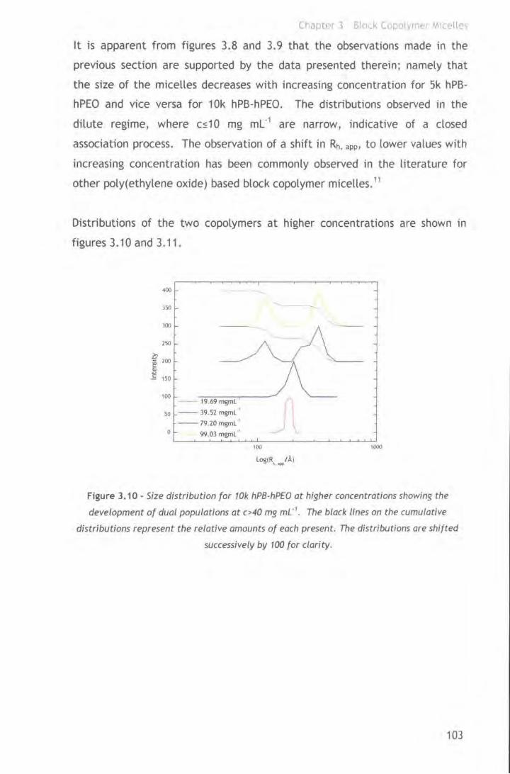
Chant£1r 3 Bloc.k Coool\ mer M1rellec;
lt is apparent from figures 3.8 and 3. 9 that the observations made in the
previous section are supported by the data presented therein; namely that
the size of the micelles decreases with increasing concentration for 5k hPB·
hPEO and vice versa for 10k hPB·hPEO. The distributions observed in the
dilute regime, where cs10 mg ml·1 are narrow, indicative of a closed
association process. The observation of a shift in Rh, app. to lower values with
increasing concentration has been commonly observed in the literature for
other poly(ethylene oxide) based block copolymer micelles. 11
Distributions of the two copolymers at higher concentratlons are shown in
figures 3.10 and 3.11.
350
300
250
~200 i E 150
100 19.69 mgml
so --39.52 mgrnl'
--79.20 mgml' 0 99.03 mgrnl '
100 1000
l~CR /A) ·--Figure 3.10 - Size distribution for 10k hPB-hP£0 at higher concentrations showing the
development of dual populations at c>40 mg mL"1• The black lines on the cumulative
distributions represent the relative amounts of each present. The distributions ore shifted
successively by 100 for clarity.
103

Chapter 3 Block Copolvme1 MKetle'i
..00
350 ---300
250
~ 200 ~ E 150
100 - 19.71 mgml '
50 --39. 55 mgml '
- 79.50 mgml ' 0 99.51 mgml'
10 100 1000 10000
Log(R,_ ,..,I A)
Figure 3.11 -Log normal size distribution for 10k hPB-hP£0 at higher concentrations showing
the development of dual populations at c>20 mg mC1• The black tines on the cumulative
distributions represent the relative amounts of each present. The distributions are shifted
successively by 100 for clarity
From figures 3.10 and 3.11 it can be seen that micelles of both copolymers
exist in bimodal distributions at higher concentrations. For 1 Ok hPB-hPEO this
occurs when c>4 mg ml·1 with the smaller size population having a radius of
ea 11 OA and the larger populations 330A. The relative occurrence of the two
populations is ea. 1:3 in favour of the larger population. lt is worthwhile
pointing out that this dual population is not always observed at these
concentrations, although it is more prevalent than the monomodal case. For
5k hPB-hPEO, the situation is a little different. Bimodal populations are
observed at c>2mg ml·1 with the smaller species having a radius of ea 110A
and the larger species between 600 and 1 oooA depending upon the
concentration. The dimensions of the larger population are more akin to
those of micellar clusters observed by Xu et a/.7 for poly(styrene)
poly(ethylene oxide). The relative occurrence for these populations is ea 3:2
in favour of the smaller populations.
One possible reason for the difference in size of the micellar clusters could be
that those formed by 1 Ok hPB-hPEO may be more tightly packed due to the
attractive nature of the micelles suggested by the diffusion second virial
coefficient, whereas those formed by 5k hPB-hPEO may be more loosely
104
Chapter 3 - Block Copolymer Micelles
packed as the same parameter for this copolymer suggests micellar
interactions of a repulsive nature.
The observation of micellar clusters at higher concentrations is not entirely
unexpected since the degree of ordering in the system is expected to increase
with concentration, and with it the level of micellar interactions. These
dominate the properties of the dispersion at higher concentrations, and are
readily observable in the small-angle scattering data that will be introduced
in subsequent sections.
3.2.4. Effect of temperature
The effect of temperature upon the properties of the micelles in aqueous
solutions for both copolymers was investigated. Temperatures in the range
283-353K in 5k increments were explored. The experiments were carried out
much in the same manner as for those detailed earlier, with the exception
that for a given experiment the concentration was fixed whilst the
temperature was varied. The concentration dependence of Dapp at each
temperature was used to ascertain the micelle radius and the second virial
diffusion coefficient.
Table 3.5 details the parameters determined from the concentration
dependence of Dapp at different temperatures for polymers 1 Ok hPB-hPEO and
5k hPB-hPEO, typical examples of which are shown in figures 3.12 and 3.13.
105
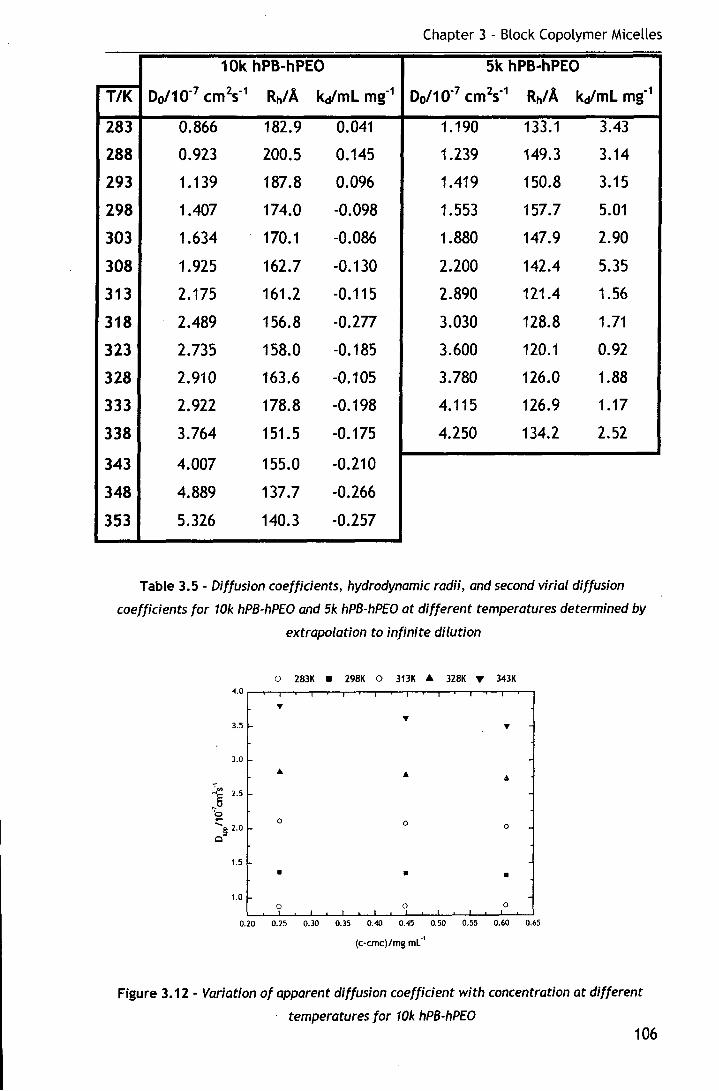
Chapter 3 - Block Copolymer Micelles
1 Ok hPB-hPEO 5k hPB-hPEO
T/K Do/1 o-7 cm2s"1 Rh/A kcll'ml mg·1 Do/1 0"7 cm2s"1 Rh/A kcll'ml mg·1
283 0.866 182.9 0.041 1.190 133.1 3.43
288 0.923 200.5 0.145 1.239 149.3 3.14
293 1.139 187.8 0.096 1.419 150.8 3.15
298 1.407 174.0 -0.098 1.553 157.7 5.01
303 1.634 170.1 -0.086 1.880 147.9 2.90
308 1.925 162.7 -0.130 2.200 142.4 5.35
313 2.175 161.2 -0.115 2.890 121.4 1.56
318 2.489 156.8 -0.277 3.030 128.8 1.71
323 2.735 158.0 -0.185 3.600 120.1 0.92
328 2.910 163.6 -0.105 3.780 126.0 1.88
333 2.922 178.8 -0.198 4.115 126.9 1.17
338 3.764 151.5 -0.175 4.250 134.2 2.52
343 4.007 155.0 -0.210
348 4.889 137.7 -0.266
353 5.326 140.3 -0.257
Table 3.5- Diffusion coefficients, hydrodynamic radii, and second virial diffusion
coefficients for 10k hPB·hPEO and Sk hPB-hPEO at different temperatures determined by
extrapolation to infinite dilution
o 283K • 298K 0 313K A 328K "f' 343K
., 3.5
3.0
0 0 0
1.5
• • • 1.0
0 0 0
0.20 0.25 0.30 0.35 OAO 0.45 0.50 0.55 0.60 0.65
(c-cmc)/mg ml·'
Figure 3.12 • Variation of apparent diffusion coefficient with concentration at different
· temperatures for 10k hPB-hPEO 106
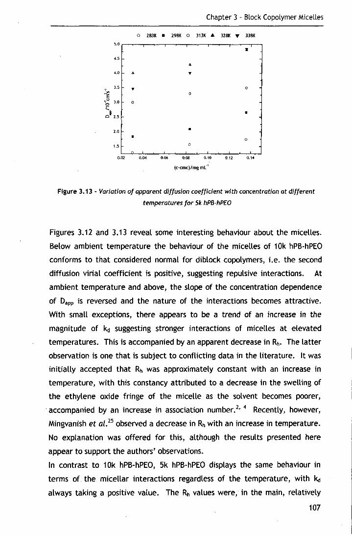
Chapter 3 - Block Copolymer Micelles
o 283K • 298K 0 313K A 328K • 338K
4.5
A
4.0 A
,. 0
0
0
•
2.0 • • 0
1.5 0
()
0.02 0.04 0.06 0.08 0.10 0.12 0.14
(c·cmc)/mg ml·'
Figure 3.13 - Variation of apparent diffusion coefficient with concentration at different
temperatures for 5k hPB-hPEO
Figures 3.12 and 3.13 reveal some interesting behaviour about the micelles.
Below ambient temperature the behaviour of the micelles of 1 Ok hPB-hPEO
conforms to that considered normal for diblock copolymers, i.e. the second
diffusion virial coefficient is positive, suggesting repulsive interactions. At
ambient temperature and above, the slope of the concentration dependence
of Dapp is reversed and the nature of the interactions becomes attractive.
With small exceptions, there appears to be a trend of an increase in the
magnitude of k<J suggesting stronger interactions of micelles at elevated
temperatures. This is accompanied by an apparent decrease in Rh. The latter
observation is one that is subject to conflicting data in the literature. lt was
initially accepted that Rh was approximately constant with an increase in
temperature, with this constancy attributed to a decrease in the swelling of
the ethylene oxide fringe of the micelle as the solvent becomes poorer,
·accompanied by an increase in association number.2'
4 Recently, however,
Mingvanish et a/. 25 observed a decrease in Rh with an increase in temperature.
No explanation was offered for this, although the results presented here
appear to support the authors' observations.
In contrast to 10k hPB-hPEO, 5k hPB-hPEO displays the same behaviour in
terms of the micellar interactions regardless of the temperature, with k<J
always taking a positive value. The Rh values were, in the main, relatively
107
Chapter 3 - Block Copolymer Micelles
constant with temperature with slight variations observed, which may be
purely due to statistical errors. This observation supports those of several
authors e.g Zhou et al. 21
3.2.5. Conclusions
For clarity, the important facts that have been concluded from the QELS data
are presented here.
• Both of the block copolymers investigated form micelles at low
concentrations, and appear to do so via a closed association process.
• The erne's were determined as 0.148 mg ml-1 for 10k hPB-hPEO and 0.268
mg mL-1 for 5k hPB-hPEO.
• Poly(butadiene) has a relative hydrophobicity that lies between that of
poly(propylene oxide) and poly(butylene oxide), an observation that is
approximately supported by an HLB calculation.
• The micelles formed have an average hydrodynamic radius of 168.A for
10k hPB-hPEO and 136.A for 5k hPB-hPEO.
• The micelles of 5k hPB-hPEO show repulsive tendencies towards each
other at all temperatures, whilst the data suggests those of 1 Ok hPB-hPEO
are attracted to one another when the temperature is at or greater than
ambient temperature.
• The micelles of 1 Ok hPB-hPEO decrease in size with an increase in
temperature, whilst those of 5k hPB-hPEO show little change in size with
temperature.
3.3. Static Light Scattering
3.3.1. Introduction
As discussed in section 2.4.2.1, SLS can be used to determine size parameters
of molecules. For homopolymers the treatment is relatively uncomplicated as
each molecule can be assumed to have the same refractive index; this is not
true for block copolymers. lt is rarely possible to synthesise block copolymers
of uniform composition. As a result, the refractive index is dependent upon
the composition. The two blocks also occupy different positions with respect
to the molecules' centre of gravity, and thus the angular distribution of
108
Chapter 3 - Block Copolymer Micelles
scattered light is different from that of a homopolymer. These two factors
have to be considered when treating light scattering data from block
copolymers.
Homopolymers can be described in terms of their molecular weight and
polydispersity index, but for block copolymers knowledge of the total
molecular weight as well as that of the individual blocks is required. If the
block copolymer is polydisperse, then account must be taken of two-fold
polydispersity, namely mass and structure. Consequently, characterisation is
somewhat complicated.
In what follows, 33 M is the molecular weight of a molecule; MA and M6 are the
molecular weights of the polymers of monomers A and B respectively. For a
monodisperse system, the composition by weight, w, of the sample is defined
by:
Equation 3.11
Similarly, for a polydisperse system, the number-average (Mn, MnA, M06
) and
weight-average (Mw, MwA, Mw6) molecular weights can be defined, with an
average composition Wn given by:
MA w = n Equation 3.12
MA+MB n n
3.3.1.1. Molecular weight
For a monodisperse homopolymer of concentration c, the excess Rayleigh
ratio, R-Ro, for an ideal solution (i.e. A2=0), is given by
Equation 3.13
P(8) is the particle scattering factor, M is molecular weight, ( ~: }s the
specific refractive index increment, c is concentration
Equation 3. 14
109

Chapter 3 - Block Copolymer Micelles
no is solvent refractive index, NA is Avogadro's number and A.o is the incident
wavelength.
As P(8) nears 1 when e approaches 0, for extrapolation of scattering intensity
to zero angle:
R-R, ~Kcu(~:)' Equation 3. 15
For a polydisperse homopolymer, having a uniform specific refractive index
increment, the molecular weight can be replaced by an average value, M:
- dn ( )
2
R-Ro =KeM de Equation 3.16
Similarly for a copolymer, an apparent average molecular weight, Mapp can be
introduced
(dn)
2
R- Ro = KeMapp de Equation 3.17
where (:). is the specific refractive index increment of the copolymer
solution. lt can either be measured experimentally, or calculated using
equation 3.18.
dn _ (dn) (dn) --WA.- +WB-de de A de B
Equation 3. 18
where (dn) is the specific refractive index increment of species i. de ;
This will be revisited in a later section.
In the case of a micellar solution, the value of c is replaced by (c-cmc) as
assuming the model of closed association, the solution at the erne can be
considered as the solvent for the micelles.
The apparent molecular weight can be related to the true value by equation
3.19:
110
Chapter 3 - Block Copolymer: Micelles
M (dn)2
=M (dn) (dn) +((dn)2
-(~n) (dn) Jw MA +((dn)2
-(dn) (dn) Jw MB w,app de w de A de B de A de A de B A w de B de A de B B W
Equation 3.19
In the case of micelles having a narrow distribution of association numbers, p,
dividing by this value gives the corresponding number-average dependence
shown in equation 3.20:
M,,._(~)' =M.(dn) (dn) +((dn)2
-(dn) (dn). JwAM: +((dn)2
-(dn) (dn) Jw8M: p de A de 8 de A de A de 8 de 8 de A de 8
Equation 3.20
3.3.2. Specific refractive index increment determination
As discussed earlier the specific refractive index increment of a block
copolymer can be related to its composition and component blocks by:34
Equation 3.21
lt is possible to measure the value of ( ddnc) directly using a differential
refractometer, or it can be calculated. Both of these approaches will be
discussed here, with the latter tackled first.
3.3.2.1. Calculation of dn/dc
The dn/dc of a given polymer is dependent upon several factors, solvent being
one of the most important, but also wavelength and temperature. As all of
the SLS measurements were carried out at 298K the effect of temperature
was not considered.
PEO is soluble in water, and thus the wavelength dependence of its dn/dc can
be readily determined from published data by a plot of dn/dc vs. 1 n.i, i.e. a
Cauchy dispersion. 34 Such a plot is shown in figure 3.14 using data from
reference. 35
111
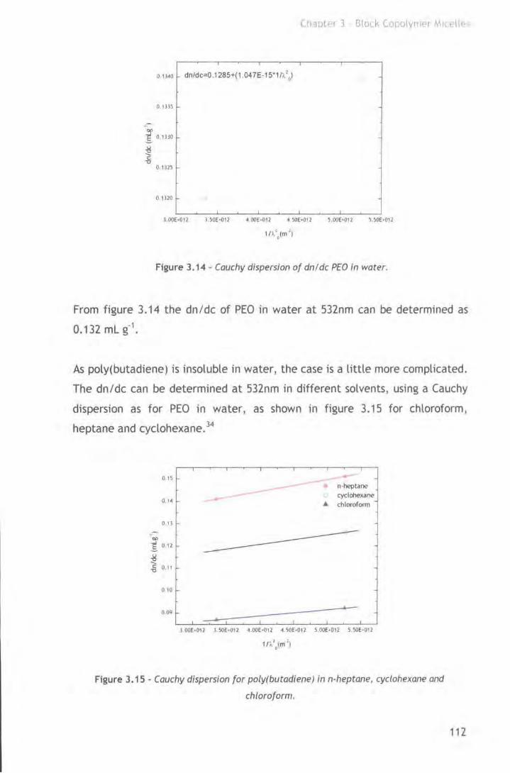
Chapter 3 Block Copolymer Mtcelle~
O. I HO dn/dc=0.1 285+(1.047E-15'1//.2 J
O. tH5
i 0.13!0
~ -5
0.1325
0 H20
l.OOE•012 ).50E~12 4 OOE•012 • 50E•012 5.00E•01l 5.50£•012
1n'.(m'')
Figure 3.14 - Cauchy dispersion of dnl dc PEO in water.
From figure 3.14 the dn/dc of PEO in water at 532nm can be determined as
0.132 ml g·1•
As poly(butadiene) is insoluble in water, the case is a little more complicated.
The dn/dc can be determined at 532nm in different solvents, using a Cauchy
dispersion as for PEO in water, as shown in figure 3.15 for chloroform ,
heptane and cyclohexane. 34
0.15
0.11
i 011
~ ..§ 0.11
010
0.09
-- n-heptane cyclohexane
A chlorofoon
3.00£·012 l .50E•012 4.00E~ll ~.50E~12 5.00E·OI2 5.50E•012
1/t.'.(m 1
)
Figure 3.15- Cauchy dispersion for poly(butadiene) in n-heptane, cyclohexane and
chloroform.
112

Chapter 3 - Block Copolymer Micelles
Interpolation of the data gives the dn/dc values at 532nm for each of the
three solvents. These are given in table 3.6 along with the refractive indices
of the respective solvents. 36
Solvent Refractive index dn/dc at 532nm/ml g·•
Cyclohexane 1.426 0.1188
Chloroform 1.446 0.0875
n-heptane 1.387 0.1420
Table 3.6- Specific refractive index increment values for poly(butadiene) at 532nm in
cyclohexane, chloroform and n-heptane determined from figure 3.15
Using equation 3.22, the dn/dc can be related to the refractive index of the
solvent: 34
Equation 3.22
Thus a plot of dn/dc vs. solvent refractive index, no, gives a slope equal to
-(dnJ , which allows determination of the dn/dc in any solvent whose de 2
refractive index is known, in this case water. Such a plot is shown in figure
3.16.
0.14
on ! 0.12
~ c: "C
0.10
dn/dc=1.3635-0.879'n0
0
1.38 1.40
0
0
1.42 1.44
Figure 3.16- Plot of dnldc vs solvent refractive index for poly(butadiene) at 532nm. The
red line is a linear fit to the data. Extrapolation to the refractive index of water (1.3329)
gives a dnldc value of 0.192 mL g·1•
113

From figure 3.16 the dn/dc of poly(butadiene) in water at 532 nm can be
determined as 0.192 ml g·1•
Using equation 3.19, this value can be considered alongside that of PEO, and
their relative contributions to the overall molecular weight of the polymer to
give its average dn/dc value. This can be calculated as 0.144 ml g·1•
The dn/dc value of the two fully hydrogenous polymers can be considered
equal, since it depends only on the composition of a molecule and is
independent of its molecular weight.
3.3.2.2. Experimental determination of dn/dc
The procedure used was outlined in section 2.5.2, producing a plot of change
in refractive index, ~n, vs. concentration, (figure 3.17), the slope of which
was the dn/dc at each different wavelength.
0.0035
0.0030
0.0025
c 0.0020 .....
0.0015
0.0010
6 3 10 12 14 16 16 20 22 2•
Con<:entration/ mgml '
Figure 3.17- Plot of change in refractive index (dn) vs concentration for 5k hPB-hPEO in
water at wavelengths of 633, 546 and 488nm, the slope of which yields the dnldc value at
the respective wavelength. The lines are fits to the data.
Using the dn/dc values calculated from figure 3.17 for the different
wavelengths a plot of dn /dc vs. 1 //...02 can be constructed (figure 3.18) as
before to allow determination of the wavelength dependence, and thus
calculation of the dn/dc at the desired wavelength.
114

Chapter 3 - Block Copolymer Micelles
0.16
0.14
0.12
"'on 0.10 E ..... ~ 0.08
c: "0 0.06
0.04
0.02
0.00 .....___.__.....___._----J.___.____. _ _._____. _ _.____, o.o 1.0x1o·• 2.0x1o·• 4.0x10~
Figure 3.18- Cauchy dispersion for Sk hPB-hPEO in water
From the relationship observed in figure 3.18, the dn/dc for the fully
hydrogenous copolymers at 532nm was dtermined as 0.137 ml g·1• This is in
reasonable agreement with the value calculated in section 3.3.2.1.
3.3.3. Molecular weight and size determination
3.3.3.1. Zimm plot method
Using the procedure described in section 2.4.2.1 SLS measurements were
carried out on polymers 10k hPB-hPEO and 5k hPB-hPEO. The dn/dc value
used was that measured experimentally in the previous section.
The Zimm plots constructed use equation 2.23 as their theoretical basis, viz.
Equation 3.23
Figures 3.19 and 3.20 show Zimm plots for 10k hPB-hPEO and 5k hPB-hPEO
respectively.
115

Chapter 3 Block Copolymer MICelles
~-OXI O
3 OXIO
on g l .OX10
~ u X
1.0X10
~ ---.... - -. ~--
Expenmental data • Extrapolated data
0.0 .___.... _ _,_ _ _.____. _ __._ _ _.__~.______J_ _ _.___._____J 0 .0 0.1 0.~ 0.6 0.8 1.0
sm1(fl/2) +100{c-<:mc)/mg ml
1
Figure 3.19- Zimm plot for 10k hPB-hP£0 in water generated using equation 3.22. Vertical
lines are fits through concentration series at a given angle and the horizontal lines are fits
through angular series at a given concentration.
Experimental Data 7.0X10 • Extrapolated data
0.0 .____._ _ _.__.._____. _ _._ _ _._____. _ ___J_ _ _.___.____,
0.0 0.2 0.4 0.6 0.8 1.0
sin1(9/ 2) +100(c-cmc)/mg ml '
Figure 3.20- Zimm plot for polymer 5k hPB-hP£0 in water generated using equation 3.22.
Vertical lines are fits through concentration series at a given angle and the horizontal lines
are fits through angular series at a given concentration.
The parameters determined from the extrapolations to zero angle and zero
concentration are listed in table 3.7.
116

Chapter 3 - Block Copolymer Micelles
10k hPB-hPEO 7.9x10°±4x10⁴ 1.216x10⁻⁴
5k hPB-hPEO 9.9x10⁶±2x10⁴ 1.872x10"4
R8, app/A
350
600
Table 3. 7 - Molecular weights, second virial diffusion coefficients (A2) and radii of gyration
calculated from extrapolated data in figures 3.19 and 3.20.
The striking feature of the data in table 3.7 is the two Rg, app values. Their
magnitudes are somewhat different to those observed in the QELS
experiments. If the micelles were acting as hard spheres then Rg:Rh-0.7737;
for the two polymers here this value is far in excess of that. A larger value of
this ratio, is usually associated with a cylindrical morphology, but small-angle
scattering data shown in later sections supports the notion that micelles are
spherical.
The 1 Ok hPB-hPEO should have the larger radii of the two due to its greater
molecular weight. The likely explanation for this is the ,shape" of the
scattering data. The radius of gyration is calculated from the limiting slope of
the extrapolation to zero concentration, which should be the lowest
horizontal line in the Zimm plot. In figure 3.20 this is clearly not the case,
and most probably leads to the erroneous value given in table 3.7. This
observation could be due to a phenomenon in the system, several examples
exist of Zimm plots exhibiting upward curvature at low angles caused by
ordering of the system. 38 The solutions used here were kept in the dilute
range to minimise such effects, and so the likely explanation is experimental
error.
In addition to the reversal in the trend of the micelle size, the apparent
molecular weights of the micelles are also the inverse of what would be
expected. Theory predicts that the association number (calculated later)
increases with the length of the hydrophobic block. 29'
39 This would mean that
the molecular weight of a micelle composed of .1 Ok hPB-hPEO would have a
higher association number, and thus molecular weight than one composed of
5k hPB-hPEO, which is clearly not the case here.
Treatment of the radius of gyration to yield the true value is more involved
than for the molecular weight, 33 and given the quality of the data it was
decided not to pursue this any further.
117

Chapter 3 - Block Copolymer Micelles
Using equation 3.18, and the dn/dc values calculated for the individual
blocks, and their respective molecular weights calculated from the Zimm
plots the true value of the micelle molecular weight can be calculated. These
values are listed in table 3.8.
Polymer Mapp/gmor 1 Mwlgmor 1
10k hPB-hPEO 7. 9x10⁶±4x10⁴ 5.88x10⁶
Sk hPB-hPEO 9. 9x10⁶±2x10⁴ 7.34x10⁶
Table 3.8 - True molecular weights of 10k and Sk hPB-hPEO calculated using equation 3. 18.
From the molecular weights determined the average association number of
the micelles can be calculated by dividing the micelle molecular weight by
that of the copolymer. The values determined are given in table 3. 9.
Polymer Mwlgmor1 p
10k hPB-hPEO 5.88x10⁶ 640
Sk hPB-hPEO 7.34x10⁶ 1657
Table 3. 9 - Association numbers, p, for 10k and Sk hPB-hPEO calculated from the molecular
weights of the micelles.
As discussed earlier the association number is expected to increase with the
length of the block forming the core of the micelle. The values determined
here are considerably higher than those obtained for poly(ethylene oxide)
copolymers of comparable molecular weight and composition, with values of
up to ea 400 being common.
In addition to the radii of gyration calculated from the data it is also possible
to estimate the micelle radius from the second virial coefficient using
equation 3.22, which has been applied by Mortensen and eo-workers. 5
Equation 3.24
These values are shown in table 3.10.
118
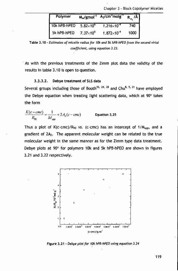
Chapter 3 - Block Copolymer Micelles
Polymer Mw/gmol"1 Az/cm~motg·• RA2/A
1 Ok hPB-hPEO 5.82x10° 1.216x10"4 740
Sk hPB-hPEO 7.37x10⁶ 1.872x10"4 1000
Table 3.10- Estimates of micelle radius for 10k and Sk hPB-hPEO from the second virial
coefficient, using equation 3.23.
· As with the previous treatments of the Zimm plot data the validity of the
results in table 3.10 is open to question.
3.3.3.2. Debye treatment of SLS data
Several groups including those of Booth 16•
24•
28 and Chu8• 9· 21 have employed
the Debye equation when treating light scattering data, which at 90° takes
the form
K ( c - cmc) 1 2A ( ) -----'----"- = --+ 2 c- cmc ~0 Mapp
Equation 3.25
Thus a plot of K(c-cmc)/R9o vs. (c-cmc) has an intercept of 1/Mapp, and a
gradient of 2A2• The apparent molecular weight can be related to the true
molecular weight in the same manner as for the Zimm typ7 data treatment.
Debye plots at 90° for polymers 1 Ok and Sk hPB-hPEO are shown in figures
3.21 and 3.22 respectively.
5 0
0
4
'"on 0
~-g 3
~ ...... a! 0 ...... u
2 ::.::
0
(c-cmc)/g mr'
Figure 3.21 - Debye plot for 10k hPB-hPEO using equation 3.24 '
119
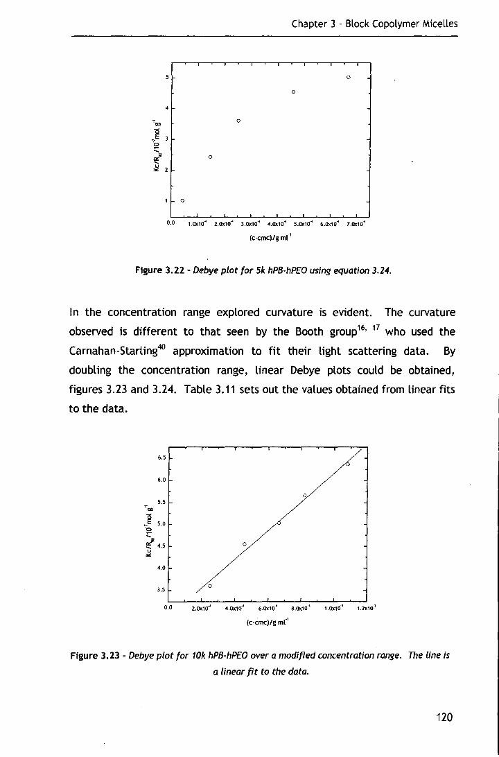
Chapter 3 - Block Copolymer Micelles
5 0
0
4
0
0
0
(c-cmc)/g mr'
Figure 3.22- Debye plot for Sk hPB-hPEO using equation 3.24.
In the concentration range explored curvature is evident. The curvature
observed is different to that seen by the Booth group16•
17 who used the
Carnahan-Starling40 approximation to fit their light scattering data. By
doubling the concentration range, linear Debye plots could be obtained,
figures 3.23 and 3.24. Table 3.11 sets out the values obtained from linear fits
to the data.
6.5
6.0
0 5.5
"'on
~~ 5.0 0
-o? - 4.5
0 u
::.::
4.0
3.5 0
0.0 2.0x10~ 4.0x10~ 6.0x10~ s.o..1o·• 1.0x10"' 1.2x10"'
(c-cmc)/g mr'
Figure 3.23- Debye plot for 10k hPB-hPEO over a modified concentration range. The line is
a linear fit to the data.
120
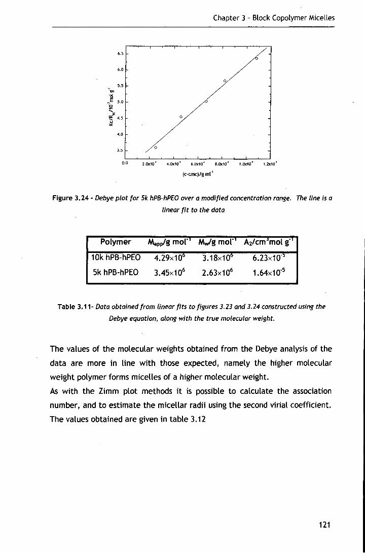
Chapter 3 - Block Copolymer Micelles
6.5 / 6.0
0 5.5
"'"on
... ] 5.0
S! ~ ..... 4.5 0
~
4.0
3.5 0
(c·cmc)/g mr'
Figure 3.24- Debye plot for Sk hPB-hPEO over a modified concentration range. The line is a
linear fit to the data
Polymer Mapplg mol" 1 Mwlg mol" 1 Az/cmJmol g·l
10k hPB-hPEO 4.29x10⁶ 3.18x10⁶ 6.23x10.:,
5k hPB-hPEO 3.45x10⁶ 2.63x10⁶ 1.64x10⁻⁵
Table 3.11- Data obtained from linear fits to figures 3.23 and 3.24 constructed using the
Debye equation, along with the true molecular weight.
The values of the molecular weights obtained from the Debye analysis of the
data are more in line with those expected, namely the higher molecular
weight polymer forms micelles of a higher molecular weight.
As with the Zimm plot methods it is possible to calculate the association
number, and to estimate the micellar radii using the second virial coefficient.
The values obtained are given in table 3.12
121

Chapter 3 - Block Copolymer Micelles
Polymer Mwlg mol"1 p
10k hPB-hPEO 3.18x10⁶ 346 6.23x10-:> 397
Sk hPB-hPEO 2.63x1 06 594 1.64x10"5 224
Table 3.12 - Association numbers, p, and estimates of the micelle radius from figures 3.23
and 3.24.
As with the previous Zimm treatment of the data, the association numbers do
not follow the pattern expected, with the lower molecular weight copolymer
having a higher association number than its . higher molecular weight
counterpart. The estimate of the micelle radius follows the pattern expected
but the values are still higher than those obtained from the QELS
experiments.
3.3.4. Conclusions
Interpretation of the data obtained during the SLS experiments is open to
question. Estimates of the sizes of the micelles are larger than those from
the QELS experiments and theoretical predictions. The association numbers
are not as expected, with the lower molecular weight polymer showing a
higher association number than its higher molecular weight counterpart.
3.4. Small-angle X-ray Scattering
3.4.1. Introduction
As discussed in section 2.4.1 small-angle X-ray scattering, (SAXS), provides a
powerful tool for probing the structure and interactions of block copolymer
micelles in solution. Unlike light scattering studies that can be performed on
relatively dilute solutions, SAXS experiments usually need higher
concentration solutions due to the lower flux of the technique. This fact
allows the micellar interactions to be probed, but also introduces
complications, as structure factors (which provide information about micellar
interactions) are described by somewhat complicated expressions. Therefore,
in order to extract the maximum amount of useful information from the data,
122

Chapter 3 - Block Copolymer Micelles
modelling techniques must be used. There are a variety of models that can
be employed, many of which have been reviewed by Pedersen and
Svaneborg,41 and Castelletto and Hamley.42
In this instance, it is the core-shell model described by Ottewill43 and
introduced in chapter two that forms the basis of the analysis of the form
factor. For the structure factor, two possible models will be considered; that
of a hard sphere based on Perkus-Yevick44-46 theory, and the mean spherical
approximation due to Hayter and Penfold.47
3.4.2. Dilute dispersions
lt was not possible to observe sufficient scattering at c<1% and so the only
data in dilute solution is that at 1%. The scattering observed for both
copolymers at this concentration was quite weak, leading to a degree of
uncertainty in the values obtained.
3.4.2.1. Preliminary analysis
Following correction of the scattering data for solvent and instrument effects,
plots of log(I(Q)) vs. log(Q) for the dilute solutions were constructed in order
to determine whether any cylindrical micelles were present. These are shown
in figure 3.25 for 1% dispersions of both 5k and 1 Ok hPB-hPEO.
g 0.1
0.01
0.01
QtJ.:'
0 0 0
0 0 oo
<D
o 10k hPB-hPEQ .A 5k hPB-hPEO
0
0.1
Figure 3.25- Log-Log plot for Sk and 10k hPB-hPEO after correcting for solvent and
instrument effects
123
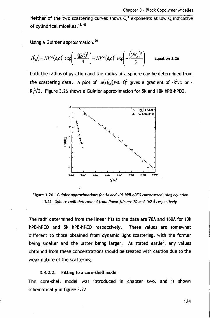
Chapter 3 - Block Copolymer Micelles
Neither of the two scattering curves shows Q-1 exponents at low Q indicative
of cylindrical micelles. 48•
49
Using a Guinier approximation:50
Equation 3.26
both the radius of gyration and the radius of a sphere can be determined from
the scattering data. A plot of In(I(Q))vs. Q2 gives a gradient of -R2 /5 or -
R/ i3. Figure 3.26 shows a Guinier approximation for 5k and 10k hPB-hPEO.
\ 0 .•
:.. --1
~ :s -2 \
-3
-4
0 0
0
0
0
0
o 10k hPB-hPE A 5k hPB-hPEO
0.000 0.001 0.002 0.003 0.004 0.005 0.006 0.007
Q'tl>:'
Figure 3.26- Guinier approximations for Sk and 10k hPB-hPEO constructed using equation
3.25. Sphere radii determined from linear fits are 70 and 160 A respectively
The radii determined from the linear fits to the data are 70A and 160A for 1 Ok
hPB-hPEO and 5k hPB-hPEO respectively. These values are somewhat
different to those obtained from dynamic light scattering, with the former
being smaller and the latter being larger. As stated earlier, any values
obtained from these concentrations should be treated with caution due to the
weak nature of the scattering.
3.4.2.2. Fitting to a core-shell model
The core-shell model was introduced in chapter two, and is shown
schematically in figure 3.27
124

Chapter 3 - Block Copolymer Micelles
Pm
Figure 3.27- Schematic representation of a core-shell particle. Re is the core radius, Res is
the micelle radius, pis the electron density, where subscript c implies the core, s implies
the shell and m the solvent.
If it is assumed that the core consists solely of PB, and the shell is dry, then:
Pc= 8.991x1010cm·2
Ps = 10.291x1010cm·2
Pm= 9.333x1010cm·2
If however the shell contains a percentage of water, as is suggested by the
SANS data (see later section), then the value of Ps consists of weighted
contributions from the two components namely PEO and H20. For this
concentration the average amount of water across the entire shell, from SANS
experiments, is 84%; this gives Ps = 9.484x1010cm·2•
In the case of a core-shell particle, the scattering can be represented by:49
J(Q)= 161r2 NPP(Q)S(Q)+B 9
where P(Q) is given by
Equation 3.27
Equation 3.28
125

Chapter 3 - Block Copolymer Micelles
Dr Richard Heenan's FISH2 analysis software51 was used to fit the
experimental data. The core-shell model used consists of nine parameters
that are detailed in table 3.13
Parameter Definition
Pe-Ps Electron density difference between core and shell
Re Core radius
Ps-Pm Electron density difference between shell and solvent
Res Total'micelle radius
Rs Shell thickness
Scale Scaling parameters based upon volume fraction
R Average core radius (see below)
J1? Standard deviation of Schultz distribution (see below)
Background Flat background added to data
Table 3.13 - Parameters used in the core-shell model utilised by the F/SH2 software.
The parameters R and J1? relate to a Schultz distribution used to allow for
micelle polydispersity. The Schultz distribution due to Kotlarchyk and Chen52
can be represented by:
Jz;f1Rzex{-(z;If] j fs(R)- fr(z +I) Equation 3.29
Z is a width parameter computed by the software.
The standard deviation, cr, of the distribution is given by:
R Equation 3.30 (]" = --:----:-:-:-:-
(z + If2
During the fitting all of the parameters listed in table 3.13 were varied, with
the exception of the two electron density differences, as allowing these to
vary produced unrealistic values for them in the final fitted parameters.
Figure 3.28 shows the fits obtained for 5k and 10k hPB-hPEO using the dry
value of the shell electron density, both in linear, and semi-logarithmic form,
with the parameters obtained given in table 3.14. 126

g
Chapter 3 Block Copolymer Mtceltt:s
4.0 a)
\ 10k hPB·hPEO
~ Sk hPB·hPEO b) 10k hPB·hPEO l
~ 5I< hPB·hPEO -1.5
1.0
2.5
20
1 5
t.O
o.s
00
0.5
a = 0.1
001 I=
I I
o.o2 o.o.t o.Ob o.oa 0.10 0.12 o.~< 0 02 0.().1 OOb o.oa 0 10 0.12 0.14
QtA' Qt/.:'
Figure 3.28 -Fits obtained to 1% dispersion data for Sk and 10k hPB-hP£0 using the FISH2
software program. a) shows a linear intensity scale, and b) shows a logarithmic intensity
scale. Lines are fits to the data
Parameter 1 Ok hPB-hPEO 5k hPB-hPEO
Re/A 13.5 59.6
Res/A 53.5 72.1
Rs/A 40 12.4
1R 0.121 0.131
Table 3.14- Parameters obtained from fits to Sk and 10k hPB-hP£0, shown in figure J.ZB,
using the core-shell model
The micelle radii obtained from these fits are somewhat smaller than those
from the light scattering studies, although the shell thickness for 5k hPB-hPEO
is somewhat questionable in relation to the value of the core given the
composition of the copolymer. As mentioned earlier the shell is likely to be
wet, containing a percentage of water. Attempts were made to fit the data
with varying the volume fraction of water, ~~ in the shell. This was achieved
by altering the electron density differences detailed in table 3.13.
Table 3.15 gives the parameters obtained for different water contents in the
shell, along with the respective electron density differences.
127
~ l } I l ' 1
i ]
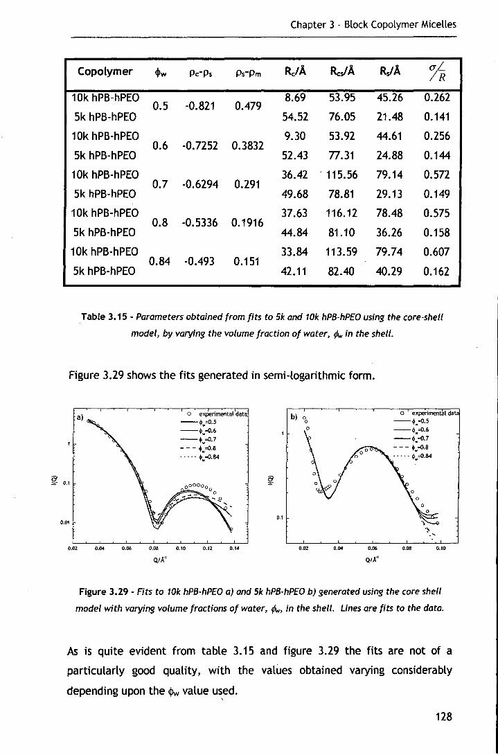
Chapter 3 - Block Copolymer Micelles
Copolymer cj)w Pc:·Ps Ps·Pm Re:! A Rc:JA RJA ~ 1 Ok hPB-hPEO
0.5 -0.821 0.479 8.69 53.95 45.26 0.262
5k hPB-hPEO 54.52 76.05 21.48 0.141
1 Ok hPB-hPEO 9.30 53.92 44.61 0.256 0.6 -0.7252 0.3832
5k hPB-hPEO 52.43 77.31 24.88 0.144
1 Ok hPB-hPEO 36.42 . 115.56 79.14 0.572 0.7 -0.6294 0.291
5k hPB-hPEO 49.68 78.81 29.13 0.149
1 Ok hPB-hPEO 37.63 116.12 78.48 0.575 0.8 -0.5336 0.1916
5k hPB-hPEO 44.84 81.10 36.26 0.158
1 Ok hPB-hPEO 33.84 113.59 79.74 0.607 0.84 -0.493 0.151
5k hPB-hPEO 42.11 82.40 40.29 0.162
Table 3.15 - Parameters obtained from fits to Sk and 10k hPB-hPEO using the core-shell
model, by varying the volume fraction of water, f/Jw in the shell.
Figure 3.29 shows the fits generated in semi-logarithmic form.
a)
g 0.1
0.01
o experimental dat -+w=O.S -+w=0.6 -+w=0,7 --- +w=0.8 ..... +w=0.84
0.1
o experimental da -+w=O.S -+w=0.6 -+w=0,7 --- +w=O.S ..... 9.=0.84
0.02 0.04 0.06 0.08 0.10 0.12 0.14 0.02 0.04 0.06
QtA''
0.08 0.10
Qt/l:'
Figure 3.29- Fits to 10k hPB-hPEO a) and Sk hPB-hPEO b) generated using the core shell
model with varying volume fractions of water, f/Jw, in the shell. Unes are fits to the data.
As is quite evident from table 3.15 and figure 3.29 the fits are not of a
particularly good quality, with the values obtained varying considerably
depending upon the IPw value used. '
128

g
Chapter 3 Block Copolymer Mtceltes
The electron densities of the three components in this system are quite
similar, and therefore the contrast is small. lt may not be possible to
distinguish between the core and the shell of the micelle because of this,
especially if the shell contains quite a large volume fraction of water, as this
reduces the contrast further.
For this reason it was decided to fit the data to a uniform sphere model.
3.4.2.3. Fitting to a uniform sphere model
The sphere model used was similar to the core-shell model in that it used a
Schultz distribution to account for polydispersity in micelle size, only this
time it was for the entire micelle, as opposed to the core. The parameters
remain much the same except the contrast factor forms part of the scaling
parameter, and the core radius is no longer present.
Figure 3.30 shows the fit generated using this model for the 10k 1% dispersion,
again in linear and semi-logarithmic form.
~.5
4.0 a) b) "
3.5 \ 3.0 \
2.S
2.0
I S
a :::- 0 .1
1.0
l o.s
0.0
·D.5 0 01 f .--'------'-__,____,____,__~ _L 1 1 I
0 02 0.~ 0.06 0 08 0.10 0.12 0 14 0.02 o.~ o.06 o.oa 0.10 0.12 o ,.
QJA.' QtA'
Figure 3.30- 10k hPB-hPEO fitted to a simple sphere model. a) Shows a linear intensity
scale, whilst b) shows a logarithmic intensity scale
The fit shown in figure 3.30 suggests a micellar radius of SSA. This is
somewhat smaller than the values suggested by light scattering. lt is evident
from figure 3.30 that the uniform sphere model does not fit the data
adequately enough, and so its use was not pursued further.
129

Chapter 3 - Block Copolymer Micelles
Because of the lack of SAXS contrast and weak scattering intensity, the 1%
dispersions of the two copolymers reveal little in terms of the micelle
dimensions. Fits to the data suggest they are spherical core-shell particles
that are approximately 150-200A in diameter.
3.4.3. Higher Concentration dispersions
When a scattering system is sufficiently dilute, or there is no long-range
ordering between the particles, then S(Q) = 1 , and the features of the
scattering are determined by P(Q). As the concentration increases, so does
the number of scattering particles and usually the degree of order in the
system. Under these conditions S(Q) * 1, and the scattering pattern becomes
more complex.
Two methods of modelling S(Q) were explored here, the first of which, based
on a hard-sphere potential, 44"46 was introduced in chapter two. The second
uses the mean spherical approximation of Hayter and Penfold. 47
3.4.3.1. Hard-sphere potential44-46
A hard-sphere potential is the simplest form of interaction between particles.
At a certain distance of separation, the energy of interaction rises steeply to
infinity, as shown in figure 3.31.
130

Chapter 3 Block Copolymer Mrcelles
, -- , ... , ""
... , " " ' ; ' ' ,
' ,
Separation distance, r , '
, ' I ' I ' I
Ol \ I
() \
I I I \ I '"
I
I
' I
I I I
I ft I I f,l I I I . \ I \ I • I I
\ . I . ' . I
' R . I . ' . , ' ;" "
. ' . , '
. ' " ' . ' . , ' -': . '--'"'{--'
: . . . . . . . . . . . r
Figure 3.31 - schematk representation of a hard-sphere interaction potential between two
spheres. R is sphere radius, RHs is the hard sphere radius.
This distance, r, can be defined as 2Rhs, where Rhs is the effective hard sphere
radius. Generally Rhs> R.
The hard sphere volume fraction, 11, is:
Equation 3.31
where V is the total volume of the system and Np is the number of particles in
the system.
The structure factor is then given by equation 3.30
S(Q) = , l 1 + 24'7( (,(2QR) 2QR)
Equation 3.32
where
131
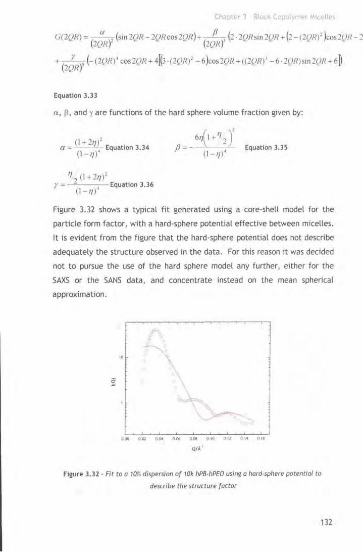
Chapter 3 Block Gopoly' <>r Mr~,.elles
G(2QR) = (2~?.Y (sin 2QR -2QRcos2QR)+ (:2tRY (2 · 2QRsin2QR + (2 -(2QR)J )cos2QR- 2
+ (2~R)5 (- (2QR)4 cos 2QR + 4[(3 ·(2QR)~ -6 }cos2QR + ((2QR)
1 -6 · 2QI?)sin 2QR + 6 D
Equat ion 3.33
a , j3, and y are functions of the hard sphere volume fraction given by:
(1+2 )~ a= 17
J Equation 3.34 (l -17)
Equation 3.35
'7 J (1 + 217) 2 •
y = -4
Equation 3.36 (1 - 17)
Figure 3.32 shows a typical fit generated using a core-shell model for the
particle form factor, with a hard-sphere potential effective between micelles.
lt is evident from the figure that the hard-sphere potential does not describe
adequately the structure observed in the data. For this reason it was decided
not to pursue the use of the hard sphere model any further, either for the
SAXS or the SANS data, and concentrate instead on the mean spherical
approximation.
10
a
0,00 0.02 0.0'1 0.06 0.08 0.10 0.12 0. H 0 16
QIA'
Figure 3.32 - Fit to a 10% dispersion of 10k hPB-hPEO using a hard-sphere potential to
describe the structure factor
132

Chapter 3 - Block Copolymer Micelles
3.4.3.2. Mean Spherical Approximation47
The mean spherical approximation was developed for charged particles in
solution but has been successfully applied to non-ionic species. 53•
54
The repulsive potential between two identical spherical macroions of
diameter, cr, is given by:
U(r) = ;rr£0£0"21f/g exp[- K(r- a))
r Equation 3.37
where eo is the permitivity of free space, E is the solvent relative permitivity,
\lfo is the surface potential, K is the Debye-Huckel inverse screening length and
r is the macroion centre-to-centre distance.
The surface potential, \lfo, can be related to the electronic charge, Zm, of the
macroion by:
z lf/o = m Equation 3.38
;rr£0£a(2 +KO")
Defining x =%, k = Ka, and K = Qa equation 3.37 can be expressed in
dimensionless units as:
f3U(x) = yexp(-kx) x > 1 Equation 3.39 X
where f3 = J{cBT, and yexp(-k) = f3;rre0&alf/g Equation 3.40
is the contact potential for a macroion pair in units of ks T.
The particle volume fraction, 11, is given by:
Equation 3.41
The structure factor can then be expressed in closed analytic form as:
1 S(Qa) = ----
1- 24qa(2Qa) Equation 3.42
where a(2Qcr) is a complex trigonometrical expansion, given in Appendix A.
Attempts were made to fit the data using the mean spherical approximation,
and typical fits can be seen in figures 3.33 to 3.36, with the associated
parameters given in tables 3.16 and 3.17.
133
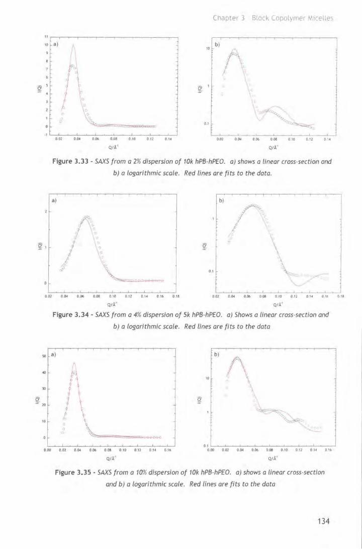
g
11,-,-~~----.-~-.----.---------~
10 a)
0.02 0.0. 0.06 0.08
QtA''
0.10 0.12 0.14
10
0.1
Chapter 3 Block Copolymer M1celles
b)
c.\ I \ I
0.02 0.04 0.06 006
QtA'
0.10 012 0 1-4
Figure 3.33 - SAXS from a 2% dispersion of 10k hPB-hPEO. a) shows a linear cross-section and
b) a logarithmic scale. Red lines ore fits to the data.
a)
0 02 0.04 0.06 0.08 0 10 0.12 0.14 0.16 0.18
b)
0.1
" \ \ \.-
0.02 0.04 0.06 0 06 0 10 0.12 0 14 0 16 0 18
QtA'
Figure 3.34- SAXS from a 4% dispersion of Sk hPB-hPEO. a) Shows a linear cross-section and
b) a logarithmic scale. Red lines ore fits to the data
so a) b)
10
lO
- 20
10
0.00 0.02 0.04 0.06 0.08 0. 10 0.12 0.14 0.1b
Q/A''
01 ~--~--~--~~~~~--~~~--~
0.00 0.02 0.04 0.06 0.06 0.10 0 12 0 14 016
QJJ<'
Figure 3.35 - SAXS from a 10% dispersion of 10k hPB-hPEO. a) shows a linear cross-section
and b) a logarithmic scale. Red lines are fits to the data
134
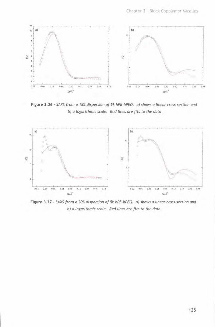
g
11r-~.---.-~-.~-.---,----r-~~~
10 a)
7
' '
o.o2 o.04 o.06 o.oa 0.10 o.12 o.t• o.16 o.1a
QJA'
Cl
Chapter 3 Block Copolymer Micelles
b )
10 ~::~~-, '(~ ,.-
\
\ \_
0.02 0.04 0.06 o.oa 0.10 0 12 o . •• 0.16
QIA'
Figure 3.36- SAXS from a 15% dispersion of 51< hPB-hPEO. a) shows a linear cross-section and
b) a logarithmic scale. Red lines are fits to the data
a) 1~ &
~
10
\ ~ ~~--
0.02 0.04 0.06 o.oa 0.10 0.12 0 14 0.16 0. 18
QtA'
10
b)
r:r.,. ~:~c>~.'
-{' ·,,.
\ l
\
oo2 o.04 006 o.oa o to 0 .12 o 1• o •• o u
QIA'
Figure 3.37- SAXS from a 20% dispersion of 51< hPB-hPEO. a) shows a linear cross-section and
b) a logarithmic scale. Red lines are fits to the data
135
l 0 1&
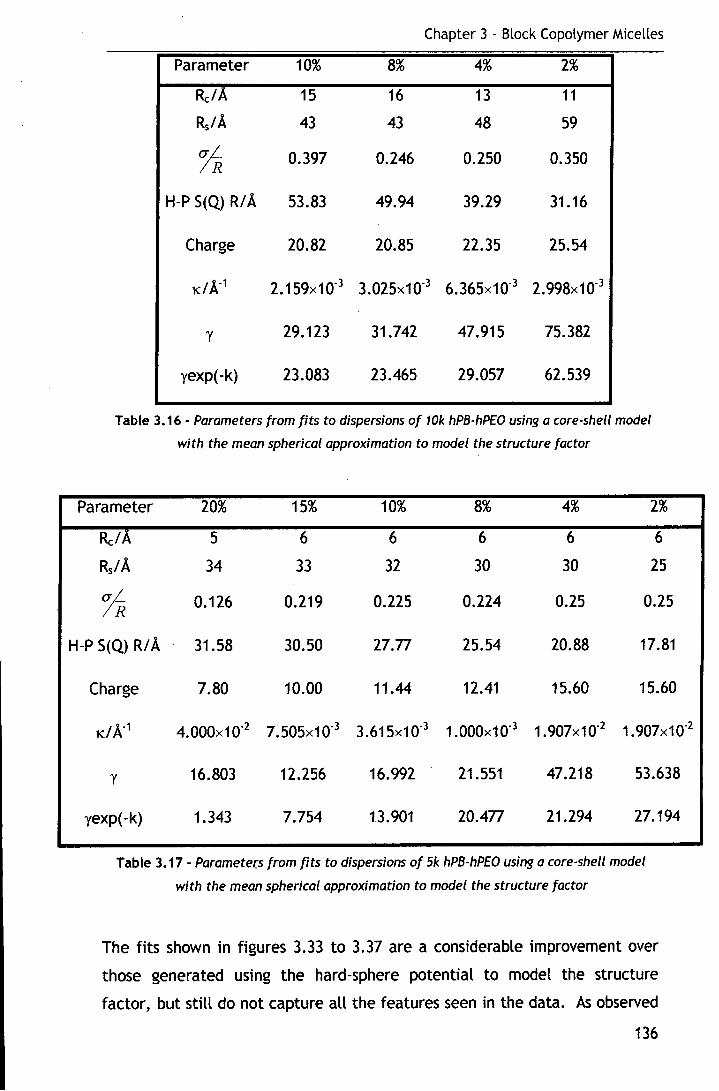
Chapter 3 - Block Copolymer Micelles
Parameter 10% 8% 4% 2%
~/A 15 16 13 11
Rs/A 43 43 48 59
1R 0.397 0.246 0.250 0.350
H-P S(Q) R/A 53.83 49.94 39.29 31.16
Charge 20.82 20.85 22.35 25.54
KIA"1 2.159x1 0"3 3.025x10"3 6.365x10"3 2.998x10"3
y 29.123 31.742 47.915 75.382
yexp(-k) 23.083 23.465 29.057 62.539
Table 3.16 - Parameters from fits to dispersions of 10k hPB-hPEO using a core-shell model
with the mean spherical approximation to model the structure factor
Parameter 20% 15% 10% 8% 4% 2%
~/A 5 6 6 6 6 6
Rs/A 34 33 32 30 30 25
1R 0.126 0.219 0.225 0.224 0.25 0.25
H-P S(Q) R/A 31.58 30.50 21.n 25.54 20.88 17.81
Charge 7.80 10.00 11.44 12.41 15.60 15.60
K/A"1 4.000x10"2 7.505x10"3 3.615x10"3 1.000x10"3 1. 907x10"2 1.907x10"2
y 16.803 12.256 16.992 21.551 47.218 53.638
yexp(-k) 1.343 7.754 13.901 20.4n 21.294 27.194
Table 3.17 - Parameters from fits to dispersions of 5k hPB-hPEO using a core-shell model
with the mean spherical approximation to model the structure factor
The fits shown in figures 3.33 to 3.37 are a considerable improvement over
those generated using the hard-sphere potential to model the structure
factor, but still do not capture all the features seen in the data. As observed
136

Chapter 3 - Block Copolymer Micelles
with the 1% dispersions, the micellar dimensions are somewhat smaller than
those observed by light scattering, likely due to the lack of SAXS contrast.
Consequently, information extracted from the fits should be treated with
caution, and perhaps assessed as qualitative rather than quantitative.
Particularly noteworthy is the shape of the scattering for the 20% dispersion of .
Sk hPB-hPEO. The structure factor peak appears to have two separate
contributions, possibly due to a higher degree of ordering than the liquid-like
structure observed at the lower concentrations.
3.4.4. Conclusions
The lack of SAXS contrast between the different components of the scattering
system hampered attempts to extract quantitative information about the size
and interactions between micelles both in dilute and more concentrated
dispersions where the interactions are more prevalent. The scattering in the
dilute regime was weak and the lowest concentration accessible was ea 1%.
Consequently, fitting the data to suitable models proved troublesome.
For clarity, the main conclusions that can be inferred from the data are
presented here.
• Micelle dimensions obtained from fits to a core-shell model at low
concentration for 1 Ok hPB-hPEO suggest a core radius of ea 14A
surrounded by a shell with a thickness of ea 40A. This suggests a micelle
radius of 54A, which is smaller than that observed by QELS and that
predicted by theory.
• The quality of the dilute dispersion data for Sk hPB-hPEO was poor due to
the weak scattering, and so it was not possible to fit the data adequately
to any model.
• A hard-sphere potential proved inadequate to model the structure factor
for the more concentrated dispersions.
• The mean spherical approximation was used to model the structure factor
for the concentrated dispersions with many but not all of the features in
the data being captured.
• Higher concentration dispersions suggest a core radius of 13A and a shell
thickness of ea SOA for 1 Ok hPB-hPEO, whilst the data for Sk hPB-hPEO
suggests a core radius of 6A and a shell thickness of ea 30A.
137
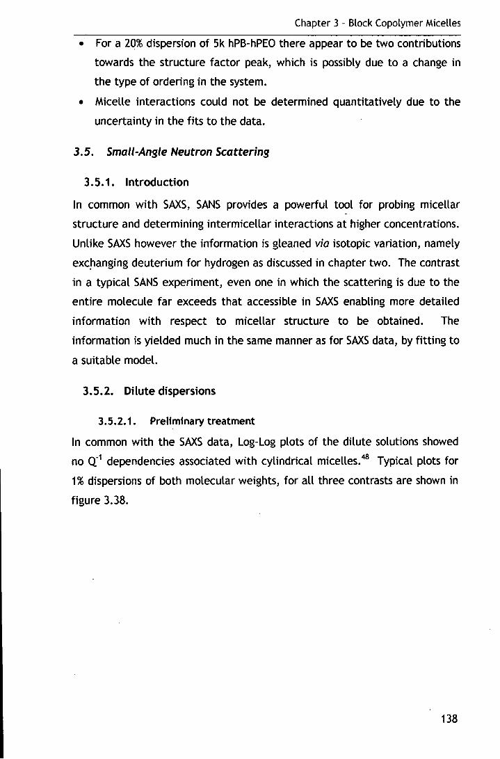
Chapter 3 - Block Copolymer Micelles
• For a 20% dispersion of 5k hPB-hPEO there appear to be two contributions
towards the structure factor peak, which is possibly due to a change in
the type of ordering in the system.
• Micelle interactions could not be determined quantitatively due to the
uncertainty in the fits to the data.
3.5. Small-Angle Neutron Scattering
3.5.1. Introduction
In common with SAXS, SANS provides a powerful tool for probing micellar
structure and determining intermicellar interactions at higher concentrations.
Unlike SAXS however the information is gleaned via isotopic variation, namely
exc~anging deuterium for hydrogen as discussed in chapter two. The contrast
in a typical SANS experiment, even one in which the scattering is due to the
entire molecule far exceeds that accessible in SAXS enabling more detailed
information with respect to micellar structure to be obtained. The
information is yielded much in the same manner as for SAXS data, by fitting to
a suitable model.
3.5.2. Dilute dispersions
3.5.2.1. Preliminary treatment
In common with the SAXS data, log-log plots of the dilute solutions showed
no Q-1 dependencies associated with cylindrical micelles.48 Typical plots for
1% dispersions of both molecular weights, for all three contrasts are shown in
figure 3.38.
138
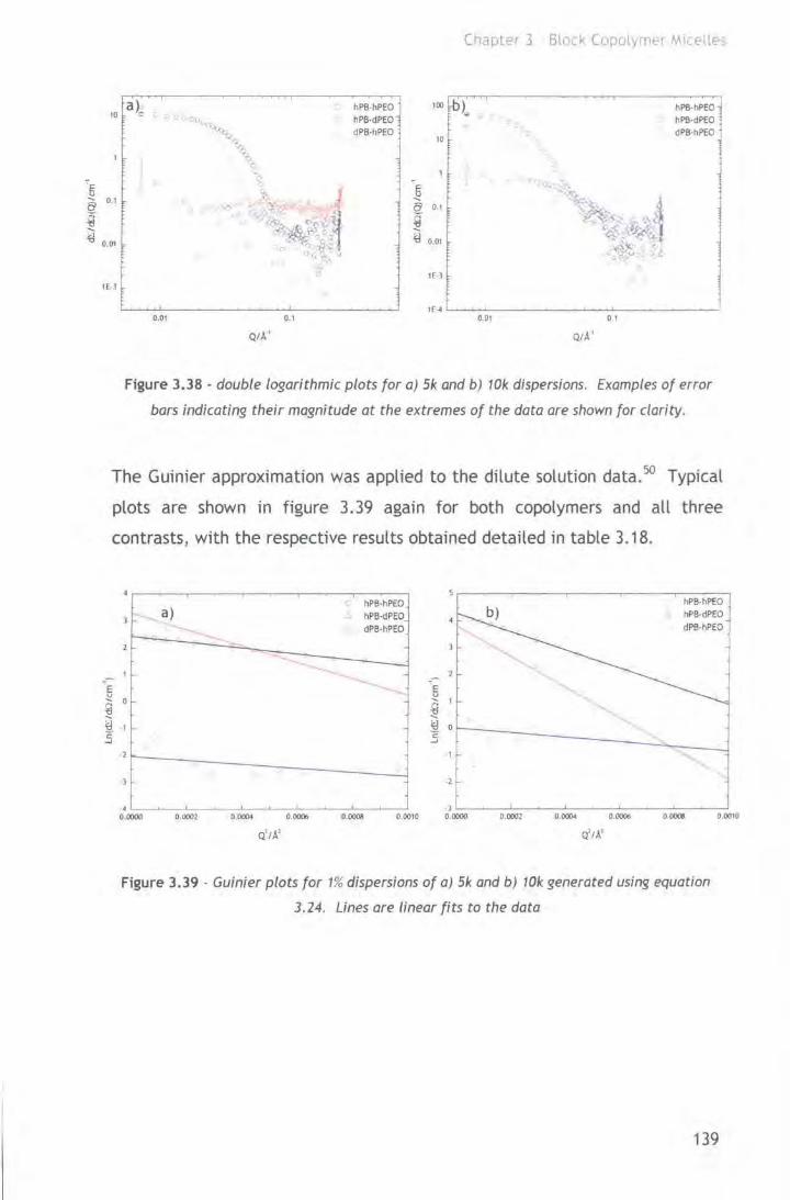
IE·l
0.01
QtA:'
0.1
hPB-hPEO hPB·dPEO dPB·hPEO
100
10
IE·J
Chapter 3 Block Copolymer M1cetles
hPB-hPEO hPB·dPEO dPB·hPEO
lE 4 '--'-~-'--------'~-'-'------....J 001 0 I
QIA'
Figure 3.38 - double logarithmic plots for a) 5k and b) 10k dispersions. Examples of error
bars indicating their magnitude at the extremes of the data are shown for clarity.
The Guinier approximation was applied to the dilute solution data. 50 Typical
plots are shown in figure 3.39 again for both copolymers and all three
contrasts, with the respective results obtained detailed in table 3.18.
E V -... D
~ ~ · I c ~
'--
• 0.0000
a)
. - --
0.0002 0 .0004 O.OOOt>
Q'tA'
hPB-hPEO hPB·dPEO dPB·hPEO
--- -....
""'
0.0008 0.0010
-2
Q'tA'
hPB·hPEO hPB·dPEO dPB·hPEO
Figure 3.39 - Guinier plots for 1% dispersions of a) 5k and b) 10k generated using equation
3.24. Lines are linear fits to the data
139

Cone/%
0.2
0.4
0.6
1
hPB-hPEO
5k. 10k
76 132
74 131
n 130
74 130
Chapter 3 - Block Copolymer Micelles
Sphere Radius/A
hPB-dPEO dPB-hPEO
5k 10k 5k 10k
126 161 n/a 56
125 173 n/a 65
120 168 48 60
. 123 169 61 66
Table 3.18 - radii determined from slopes of the linear fits to Guinier plots of the type
shown in figure 3.41 for 5k and 10k dispersions at cs't%. The part of micelle scattering
neutrons is highlighted in bold.
lt can be seen from table 3.18, that there are differences between the
micelle radii determined for the fully hydrogenous polymer and those for the
deuterated shell polymer for both molecular weights. These are likely due to
the difference in the molecular weights of the copolymers and to the
different weightings given by the contrasts factors to the individual from
factors in equation 3.27.
3.5.2.2. Fitting to a core-shell model
The greater degree of contrast available in SANS enabled the use of slightly
more sophisticated models to fit the data. For the SAXS data the polymer
volume fraction in the shell was assumed to be uniform across its entire
width. Polymer brush theory discussed in chapter one suggests this is not the
case, 55 with a decrease in volume fraction with increasing distance from the
core-shell interface being predicted. This was taken into account in the
models utilised.
The core was assumed to consist exclusively of PB, and to be of uniform
density. The volume fraction of PEO in the corona was modelled by a series
of six linear steps approximating to a parabolic profile. As a result, the
corona was essentially split into six sub-shells, each having a local
concentration profile of PEO. Figure 3.40 shows the variation of the neutron
scattering length density with distance from the micelle core for each of the
contrasts used.
140
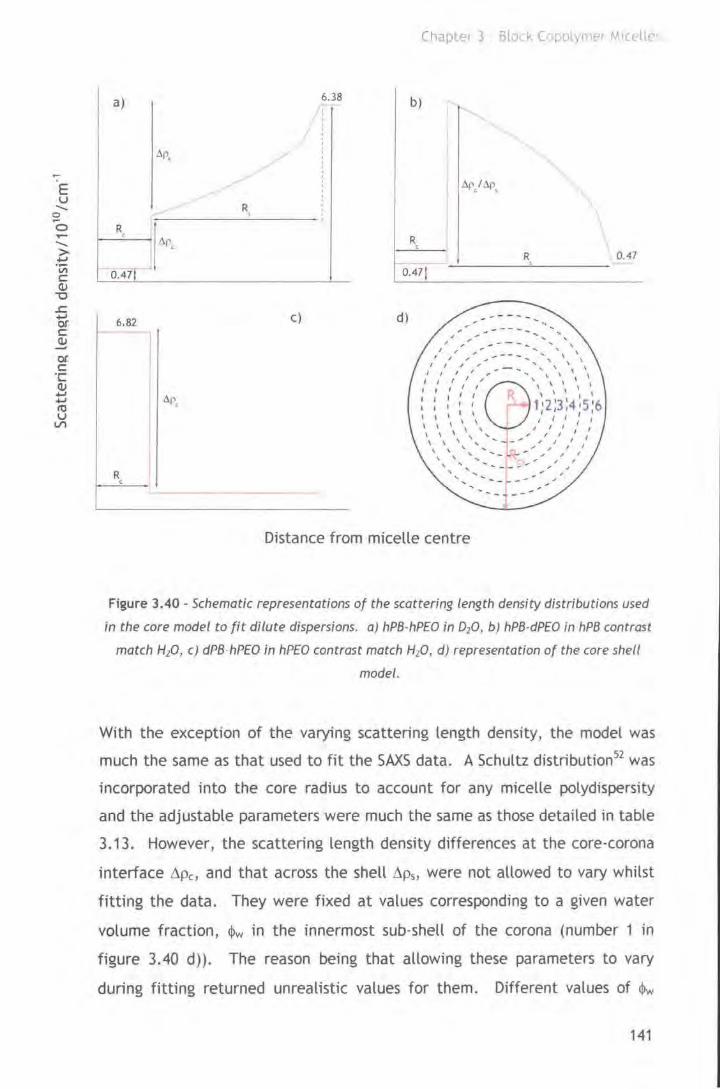
a)
R
0.47f
6.82
R '
6.38
c)
Chapter 3 Block Copolymer M'Cellt>
b)
R c
0.471
d ) ----- .... , , , , -
,' ,' ,.~ ' ....... -- ...... ' \
I f / / .,... -.., ' ... \ \ \ I 1 I ' , , \. \ \ \
I I I I / \ \ \ 111''0 '',•' I I \ \ t t
: : : I I 1;2;3:415;6 I I I \ \ I I I I I \ \ \ \ \ 1 I I I 1
\ \ \ \ ' / I I I I \ \ \ ' ...._ --,... , I I
\ ' "- , ,> 1 1 I
\ ', ' .... _ .... - ....... : ....... , ' ,' ' ' .... ___ , , ', .... ___ ,_.,"' ., '
0.47
Distance from micelle centre
Figure 3.40 - Schematic representatjons of the scattering length density distributions used
in the core model to fit dilute dispersions. a) hPB-hP£0 in 020, b) hPB-dPEO in hPB contrast
match H10 , c) dPB·hP£0 in hPEO contrast match H10 , d) representation of the core shell
model.
With the exception of the varying scattering length density, the model was
much the same as that used to fit the SAXS data. A Schultz distribution52 was
incorporated into the core radius to account for any micelle polydispersity
and the adjustable parameters were much the same as those detailed in table
3.13. However, the scattering length density differences at the core-corona
interface .1pc, and that across the shell .1p5 , were not allowed to vary whilst
fitting the data. They were fixed at values corresponding to a given water
volume fraction, ~ in the innermost sub-shell of the corona (number 1 in
f igure 3.40 d)). The reason being that allowing these parameters to vary
during fitting returned unrealistic values for them. Different values of <Pw
141
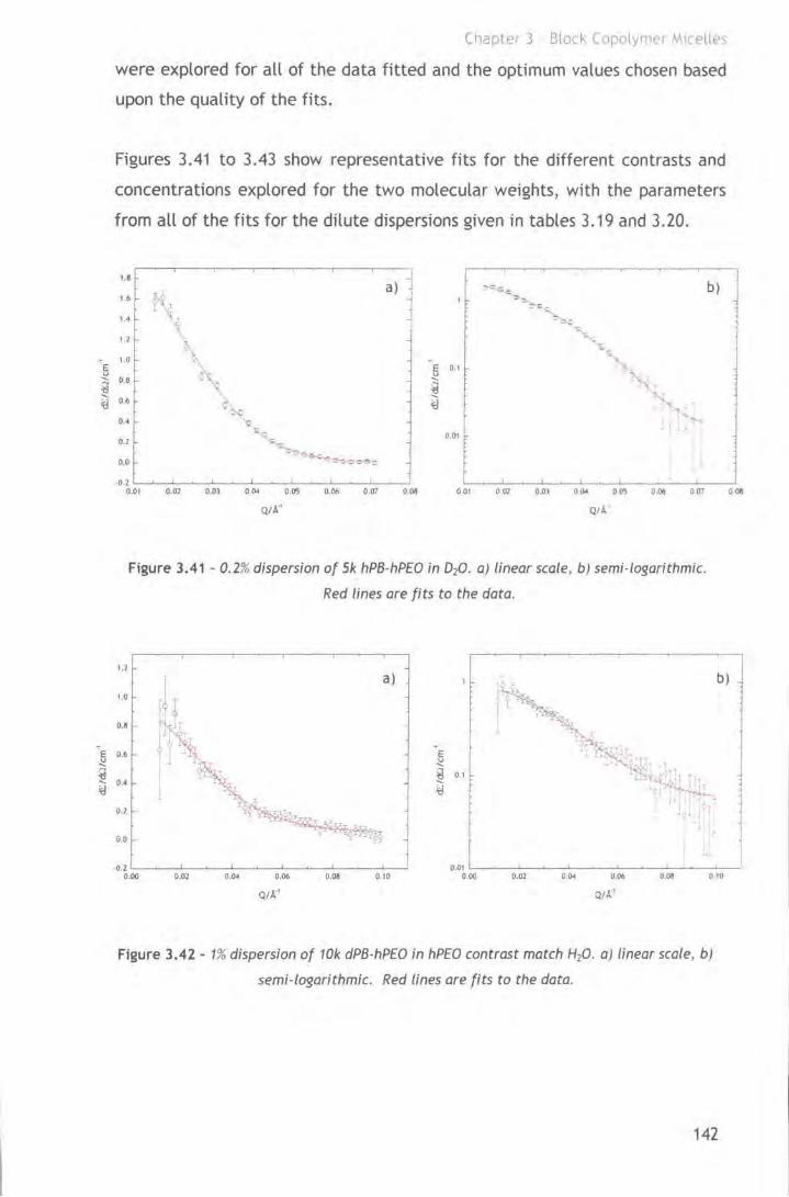
' E V
~ ~
E V
~ ~
Chapter 3 Block Copolymer MKelles
were explored for all of the data fitted and the optimum values chosen based
upon the quality of the fits.
Figures 3.41 to 3.43 show representative fits for the different contrasts and
concentrations explored for the two molecular weights, with the parameters
from all of the fits for the dilute dispersions given in tables 3.19 and 3.20.
1.8
~~~ a) e--=.::..e b)
1.1> ~~ ~<:.:
1.4 \~ :>I!>:
~-I 1
\ .... :;
";
1.0
~ E 0.1
H. V 0.8 .....
~ 0.6 - ~ ~--....
-~ 0.4 l: "N
0.1 1;.::
$."" 0 01
0.0 ·~oo-c.
e~--= o-'0;-
·O.l 0.01 O.Ol 0.03 0.04 O.O'i 0.01> 0.117 o.oa 0 01 001 O.Ol 0.04 00'; 006 0.07
Q/A·' Q!A '
Figure 3.41 - 0.2% dispersion of Sk hPB-hP£0 in 020. a) linear scale, b) semi-logarithmic.
I 2
1.0
0.8
0.6
0.4
0.2
00
0.2 0.00 0.02 0.04 0.06
QIA'
Red lines are fits to the data.
a)
o.oa 0.10 0.02 0.04 0.06
QIA"'
o.oa 010
Figure 3.42- 1% dispersion of 10k dPB-hP£0 in hP£0 contrast match H20. a) linear scale, b)
semi-logarithmic. Red lines are fits to the data.
142
ooa

18
16
14
12
' E 10
~ a ~ 4:) 6
1
Chopter 3 Block Copolymt~r ~'" ellE>s
a) b) •• 10 • • ~ ..
"' • .,
!:" E ~ :l
~ ~ -=-"' . --r/- ... "t:l 0 t ..,
• .. .... ~~.~ .. ~··•+++• 0.01
0 01 0 02 0.03 0.04 0.05 0.06 001 0.01 O.OJ 004 OO'l oar
QtA ' QIA
Figure 3.43 - 0.6% dispersion of 10k hPB-dPEO in hPB contrast match H20. a) linear scale, b)
semi-logarithmic Red lines are fits to the data .
Copolymer Cone/% ReA RsA .1pc/1 o10cm·2 .1pJ1010cm·2 a/.-/ R ~
hPB-hPEO 0.2 21 67 -5.049 -0.861 0.225 0.85
0.4 19 62 -4.877 -1.033 0.463 0.82
0.6 19 59 -4.762 -1 .148 0.502 0.8
1.0 20 58 -4.590 -1.320 0.468 0.77
hPB-dPEO 0.2 24 97 -0.898 0.898 0.371 0.85
0.4 24 96 -1.078 1.078 0.456 0.82
0.6 25 93 -1.198 1.198 0.465 0.80
1.0 25 91 ·1.198 1.198 0.455 0.80
dPB-hPEO 0.2
0.4 Scattering too weak to fit
0.6
1.0 27 6.180 0 0.009
Table 3.19 - Parameters obtained from 5k dispersions fitted to the core model shown in
figure 3.40, using FISH 2with the parameters as detailed therein.
143
I

Chapter 3 - Block Copolymer Micelles
Copolymer Cone/% ReA RsA Apc/1010cm·2 ApJ101ucm·" 1R ~
hPB-hPEO 0.2 35 115 -5.049 -0.861 0.1 0.85
0.4 40 108 -4.877 -1.033 0.35 0.82
0.6 39 112 -4.475 -1.435 0.35 0.80
1.0 38 113 -4.647 -1.263 0.36 0.78
hPB-dPEO 0.2 40 118 -0.899 0.899 0.15 0.85
0.4 44 110 -1.078 1.078 0.15 0.82
0.6 42 113 -1.198 1.198 0.17 0.80
1.0 45 107 -1.318 1.318 0.2 0.78
dPB-hPEO 0.2 46 6.18 0.2
0.4 46 6.18 0.2
0.6 47 6.18 0.2
1.0 45 6.18 0.2
Table 3.20- Parameters obtained from 10k dispersions fitted to the core model shown in
figure 3.40, using FISH 2with the parameters as detailed therein.
From tables 3.19 and 3.20 it is evident that the total micelle radius for the 5k
series is of the between 80 and 120A, with the core radius being circa 25A.
The former is slightly smaller than the value of 136A determined by QELS
measurements in section 3.2.2, but is in reasonable agreement. The 10.k
series shows a micelle radius of 150A, again slightly smaller than the value of
168A from QELS measurements but still with reasonable agreement, whilst a
core radius of circa 40A is observed.
The goodness of the fits obtained using FISH was assessed using intensity
calculations. The. volume fractions of PB and PEO from any given fit can be
calculated and compared to the values expected from the original
composition and concentration. The closeness of these values provides an
indication as to the goodness of fit. Table 3.21 details the results of such
calculations for the fits on the dilute solutions.
144

Chapter 3 - Block Copolymer Micelles
Polymer Cone/% ~psa ~PBb ~PEOa ~PE0°
0.2 0.00041 0.00040 0.00189 0.00146
5k hPB- 0.4 0.00072 0.00080 0.00290 0.00292
hP EO 0.6 0.00088 0.00110 0.00346 0.00438
1 0.00160 0.00199 0.00693 0.00729
0.2 0.00016 0.00031 0.00179 0.00153
5k hPB- 0.4 0.00045 0.00063 0.00293 0.00305
dPEO 0.6 0.00111 0.00094 0.00424 0.00458
1 0.00156 0.00157 0.00958 0.00763
5k dPB-1 0.00104 0.00115 - -
hP EO
0.2 0.00051 0.00036 0.00195 0.00149
10k hPB- 0.4 0.00099 0.00071 0.00341 0.00299
hP EO 0.6 0.00119 0.00107 0.00561 0.00448
1 0.00185 0.00178 0.00868 0.00747
0.2 0.00040 0.00048 0.00178 0.00139
10k hPB- 0.4 0.00085 0.00097 0.00323 0.00278
dPEO 0.6 0.00137 0.00145 0.00814 0.00834
1 0.00243 0.00242 0.00571 0.00695
0.2 0.00016 0.00027 - -10k dPB- 0.4 0.00053 0.00055 - -
hPEO 0.6 0.00079 0.00082 - -1 0.00135 0.00137 - -
Table 3.21 -Comparison of calculated a and experimental b volume fractions from dilute
dispersions of the two molecular weight series
lt is evident from the values in table 3.11 that the observed and calculated
volume fractions are in good agreement suggesting that the fits are
acceptable in terms of the parameters they give.
The unperturbed radius of gyration, Rg, of a PEO chain in water at 198K can
be calculated using equation 3.42. 56
145

Chapter 3 - Block Copolymer Micelles
Equation 3.43
Table 3.22 details the values calculated for the copolymers used here.
Isotopic variation
5k hPB-hPEO
5k hPB-dPEO
5k dPB-hPEO
5k hPB-hPEO
5k hPB-dPEO
5k dPB-hPEO
Mw PEO/gmorl
3590
4295
5790
7610
4340
9230
R8 PEO/A
23
26
30
36
26
40
Table 3.22 - Unperturbed radii of gyration of PEO blocks in copolymers calculated using
equation 3.42
The number of copolymer chains in a micelle, the association number, p, can
be calculated using equation 3.43,4 assuming that the core consists solely of
PB.
~?rR; p = Equation 3.44
VPB
where Vp6 is the volume of the poly(butadiene) block given by:4
Equation 3.45
mp6 is the molecular weight of the polybutadiene block, PPB is the density of
poly(butadiene), 35 0.964 gcm·3 and NA is Avogadro's number.
The distance between PEO chains on the core surface, OpEO, can be calculated
using equation 3.45: 54
Equation 3.46
146
Chapter 3 - Block Copolymer Micelles
Tables 3.23 and 3.24 give the values of the association number, the
separation distance of the PEO chains on the core surface, and the ratio of
the shell thickness to the unperturbed radius of gyration, Rs:Rg, for both
copolymer series.
Copolymer Cone/% p OpE()/ A Rs:R.g
hPB-hPEO 0.2 27 14.39 2.88
0.4 20 15.13 2.66
0.6 20 15.13 2.53
1.0 23 14.75 2.49
hPB-dPEO 0.2 40 13.44 3.75
0.4 40 13.44 3.71
0.6 45 13.17 3.60
1.0 45 13.17 3.52
dPB-hPEO 1.0 74 - -
Table 3.23- Values of association number, p, distance between PEO chains on the core
surface DPEo, and the ratio of the shell thickness to the unperturbed radius of gyration Rs:Rg
for dilute dispersions of the Sk series.
Copolymer Cone/% p OpEofA Rs:R8
hPB-hPEO 0.2 71 14.73 3.17
0.4 106 13.78 2.98
0.6 98 13.96 3.09
1.0 91 14.14 3.12
hPB-dPEO 0.2 130 12.45 4.48
0.4 173 11.87 4.18
0.6 150 12.15 4.29
1.0 185 11.74 4.06
dPB-hPEO 0.2 213 - -0.4 213 - -0.6 227 - -
1.0 200 - -
Table 3.24- Values of association number, p, distance between PEO chains on the core
surface DPEo, and the ratio of the shell thickness to the unperturbed radius of gyration Rs:Rg
for dilute dispersions of the 10k series.
147
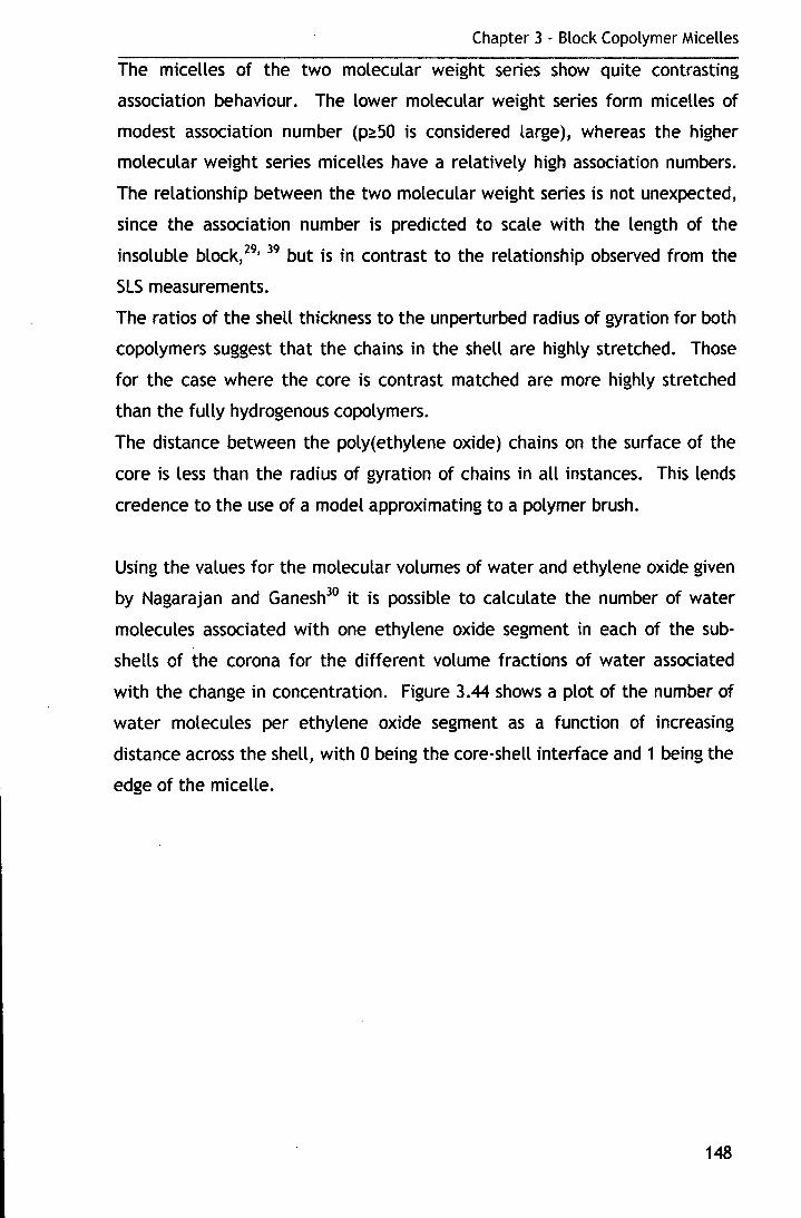
Chapter 3 - Block Copolymer Micelles
The micelles of the two molecular weight series show quite contrasting
association behaviour. The lower molecular weight series form micelles of
modest association number (p~50 is considered large), whereas the higher
molecular weight series micelles have a relatively high association numbers.
The relationship between the two molecular weight series is not unexpected,
since the association number is predicted to scale with the length of the
insoluble block/9'
39 but is in contrast to the relationship observed from the
SLS measurements.
The ratios of the shell thickness to the unperturbed radius of gyration for both
copolymers suggest that the chains in the shell are highly stretched. Those
for the case where the core is contrast matched are more highly stretched
than the fully hydrogenous copolymers.
The distance between the poly(ethylene oxide) chains on the surface of the
core is less than the radius of gyration of chains in all instances. This lends
credence to the use of a model approximating to a polymer brush.
Using the values for the molecular volumes of water and ethylene oxide given
by Nagarajan and Ganesh30 it is possible to calculate the number of water
molecules associated with one ethylene oxide segment in each of the sub
shells of the corona for the different volume fractions of water associated
with the change in concentration. Figure 3.44 shows a plot of the number of
water molecules per ethylene oxide segment as a function of increasing
distance across the shell, with 0 being the core-shell interface and 1 being the
edge of the micelle.
148
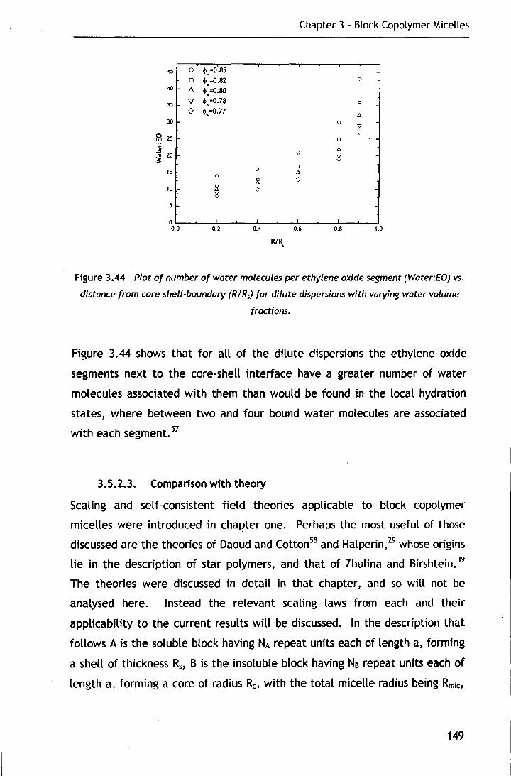
Chapter 3 - Block Copolymer Micelles
45 0 <jlw =0.85 0 <jlw =0.82 0
40 A <jlw=O.BO
35 \1 <jlw=0.78 0
<> <jlw=O.n .0. 30 0
"V
0 25 LU
(
D t.: .2!
20 ~
0 .0.
8 15 0
0 .0.
0 H .·.
V
10 • B 8
5
0 0.0 0.2 0.4 0.6 0.8 1.0
R/R '
Figure 3.44- Plot of number of water molecules per ethylene oxide segment (Water:EO) vs.
distance from core shell-boundary (RIRs) for dilute dispersions with varying water volume
fractions.
Figure 3.44 shows that for all of the dilute dispersions the ethylene oxide
segments next to the core-shell interface have a greater number of water
molecules associated with them than would be found in the local hydration
states, where between two and four bound water molecules are associated
with each segment. 57
3.5.2.3. Comparison with theory
Scaling and self-consistent field theories applicable to block copolymer
micelles were introduced in chapter one. Perhaps the most useful of those
discussed are the theories of Daoud and Cotton 58 and Halperin, 29 whose origins
lie in the description of star polymers, and that of Zhulina and Birshtein. 39
The theories were discussed in detail in that chapter, and so will not be
analysed here. Instead the relevant scaling laws from each and their
applicability to the current results will be discussed. In the description that
follows A is the soluble block having NA repeat units each of length a, forming
a shell of thickness R5, B is the insoluble block having Ns repeat units each of
length a, forming a core of radius Re, with the total micelle radius being Rmic,
149
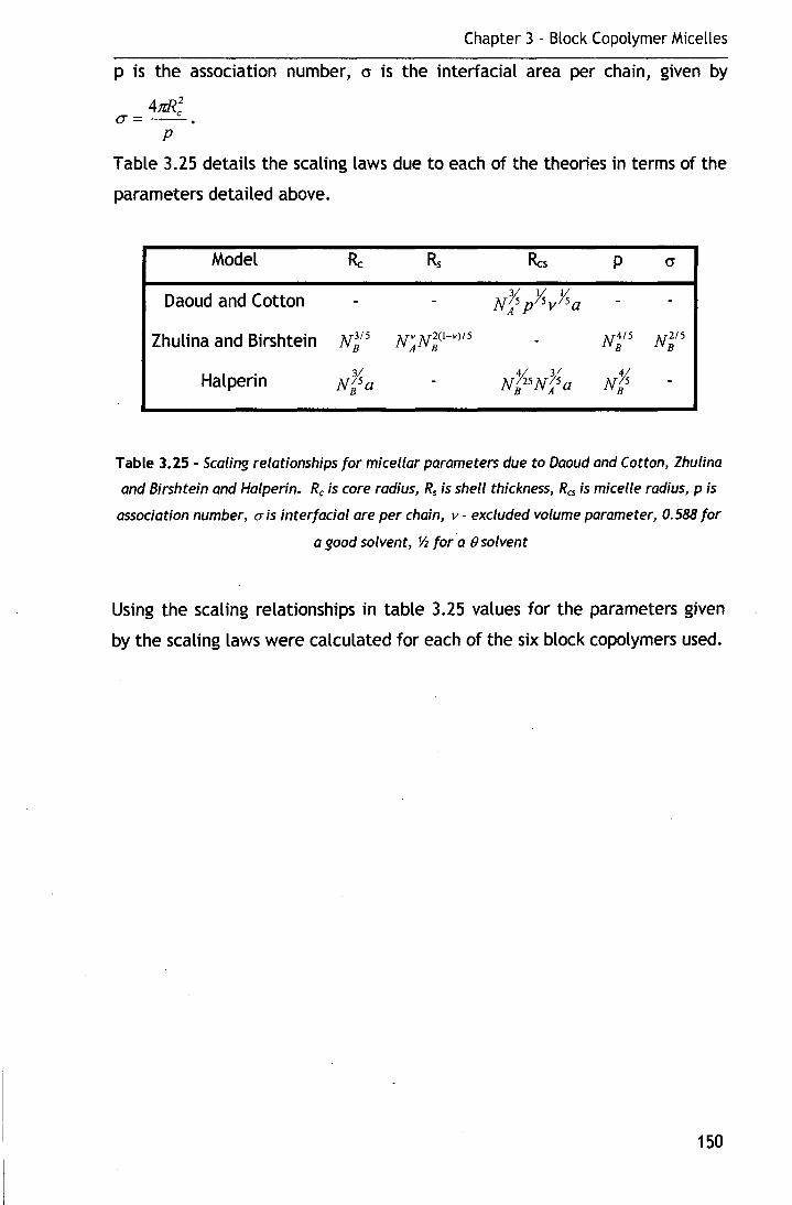
Chapter 3 - Block Copolymer Micelles
p is the association number, cr is the interfacial area per chain, given by
47d?..2 cr=--c.
p
Table 3.25 details the scaling laws due to each of the theories in terms of the
parameters detailed above.
Model Re Rs Res p cr
Daoud and Cotton Nfs pYsvYsa
Zhulina and Birshtein N3;s B
Nv N2(1-v)/5 A B
N4;s B
N21s B
Halperin NYsa % 3' N'Ys N 25 Nl5a
B B A B
Table 3.25- Scaling relationships for micellar parameters due to Daoud and Cotton, Zhulina
and Birshtein and Halperin. R, is core radius, Rs is shell thickness, Res is micelle radius, p is
association number, CTis interfacial are per chain, v- excluded volume parameter, 0.588 for
a good solvent, ~fora (}solvent
Using the scaling relationships in table 3.25 values for the parameters given
by the scaling laws were calculated for each of the six block copolymers used.
150
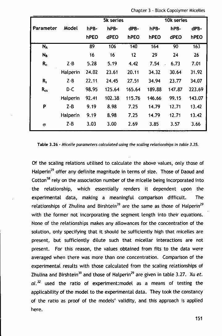
Chapter 3 - Block Copolymer Micelles
Sk series 10k series
Parameter Model hPB- hPB- dPB- hPB- hPB- dPB-
hP EO dPEO hP EO hPEO dPEO hPEO
NA 89 106 140 164 90 163
Ns 16 16 12 29 24 26
Re Z-B 5.28 5.19 4.42 7.54 6.73 7.01
Halperin 24.02 23.61 20.11 34.32 30.64 31.92
Rs Z-B 22.11 24.45 27.51 34.94 23.77 34.07
Res D-C 98.95 125.64 165.64 189.88 147.87 223.69
Halperin 92.41 102.38 115.76 146.66 99.15 143.07
p Z-B 9.19 8.98 7.25 14.79 12.71 13.42
Halperin 9.19 8.98 7.25 14.79 12.71 13.42
0' Z-B 3.03 3.00 2.69 3.85 3.57 3.66
Table 3.26- Micelle parameters calculated using the scaling relationships in table 3.25.
Of the scaling relations utilised to calculate the above values, only those of
Halperin29 offer any definite magnitude in terms of size. Those of Daoud and
Cotton58 rely on the association number of the micelle being incorporated into
the relationship, which essentially renders it dependent upon the
experimental data, making a meaningful comparison difficult. The
relationships of Zhulina and Birshtein39 are the same as those of Halperin29
with the former not incorporating the segment length into their equations.
None of the relationships makes any allowances for the concentration of the
solution, only specifying that it should be sufficiently high that micelles are
present, but sufficiently dilute such that micellar interactions are not
present. For this reason, the values obtained from fits to the data were
averaged when there was more than one concentration. Comparison of the
experimental results with those calculated from the scaling relationships of
Zhulina and Birshtein39 and those of Halperin29 are given in table 3.27. Xu et.
al. 32 used the ratio of experiment: model as a means of testing the
applicability of the model to the experimental data. They took the constancy
of the ratio as proof of the models' validity, and this approach is applied
here.
151
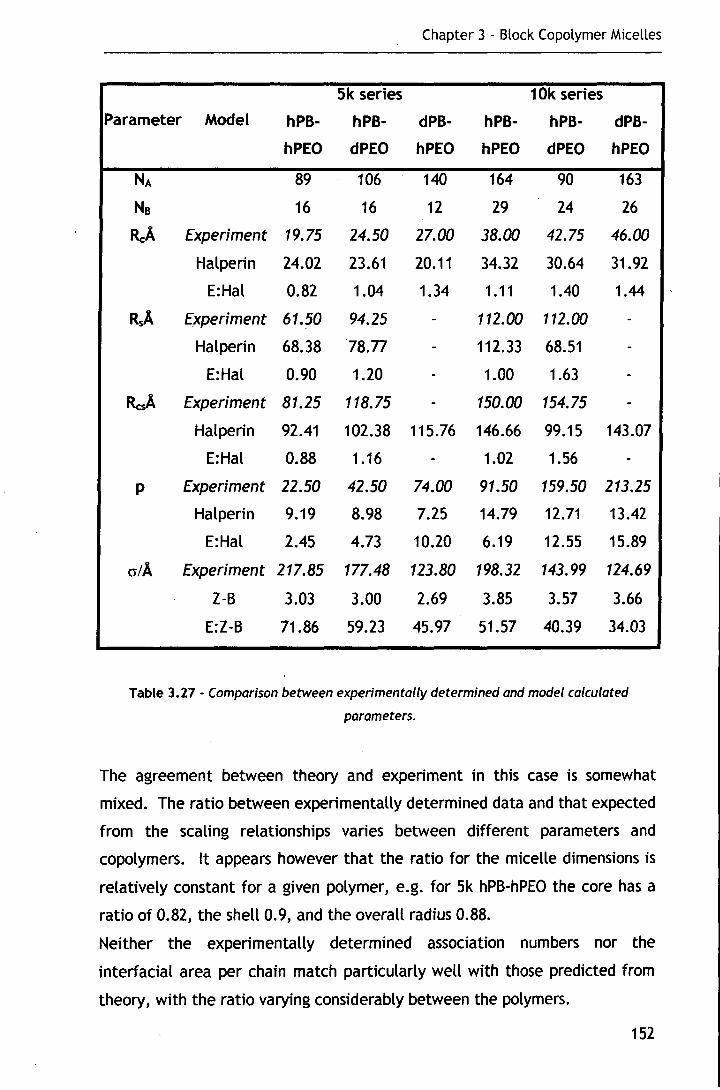
Chapter 3 - Block Copolymer Micelles
Sk series 10k series
Parameter Model hPB- hPB- dPB- hPB- hPB- dPB-
hP EO dPEO hP EO hP EO dPEO hP EO
NA 89 106 140 164 90 163
Ne 16 16 12 29 24 26
ReA Experiment 19.75 24.50 27.00 38.00 42.75 46.00
Halperin 24.02 23.61 20.11 34.32 30.64 31.92
E:Hal 0.82 1.04 1.34 1.11 1.40 1.44
RsA Experiment 61.50 94.25 - 112.00 112.00 -Halperin 68.38 '78.n - 112.33 68.51 -
E:Hal 0.90 1.20 - 1.00 1.63 -
RcsA Experiment 81.25 118.75 - 150.00 154.75 -
Halperin 92.41 102.38 115.76 146.66 99.15 143.07
E:Hal 0.88 1.16 - 1.02 1.56 -p Experiment 22.50 42.50 74.00 91.50 159.50 213.25
Halperin 9.19 8.98 7.25 14.79 12.71 13.42
E:Hal 2.45 4.73 10.20 6.19 12.55 15.89
er/A Experiment 217.85 177.48 123.80 198.32 143.99 124.69
Z-B 3.03 3.00 2.69 3.85 3.57 3.66
E:Z-B 71.86 59.23 45.97 51.57 40.39 34.03
Table 3.27- Comparison between experimentally determined and model calculated
parameters.
The agreement between theory and experiment in this case is somewhat
mixed. The ratio between experimentally determined data and that expected
from the scaling relationships varies between different parameters and
copolymers. lt appears however that the ratio for the micelle dimensions is
relatively constant for a given polymer, e.g. for 5k hPB-hPEO the core has a
ratio of 0.82, the shell 0. 9, and the overall radius 0.88.
Neither the experimentally determined association numbers nor the
interfacial area per chain match particularly well with those predicted from
theory, with the ratio varying considerably between the polymers.
152
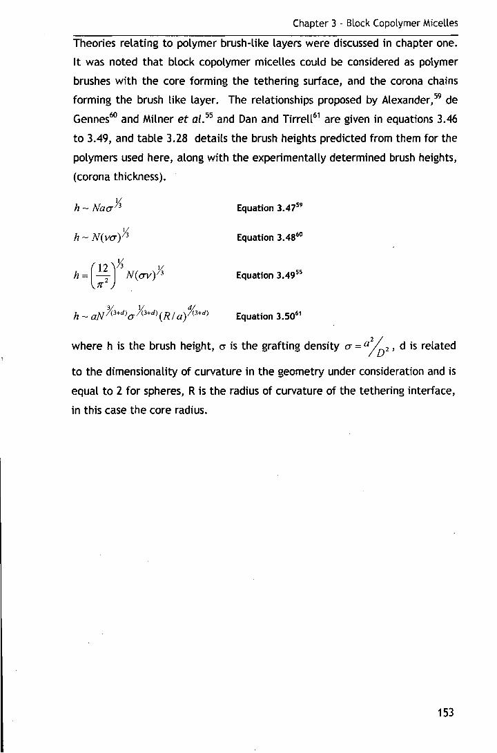
Chapter 3 - Block Copolymer Micelles
Theories relating to polymer brush-like layers were discussed in chapter one.
lt was noted that block copolymer micelles could be considered as polymer
brushes with the core forming the tethering surface, and the corona chains
forming the brush like layer. The relationships proposed by Alexander, 59 de
Gennes60 and Milner et al. 55 and Dan and Tirrell61 are given in equations 3.46
to 3.49, and table 3.28 details the brush heights predicted from them for the
polymers used here, along with the experimentally determined brush heights,
(corona thickness).
h-Naa~ Equation 3.4759
h- N(va)~ Equation 3.4860
Equation 3.4955
Equation 3.5061
where h is the brush height, cr is the grafting density a = a%2 , d is related
to the dimensionality of curvature in the geometry under consideration and is
equal to 2 for spheres, R is the radius of curvature of the tethering interface,
in this case the core radius.
153

Chapter 3 - Block Copolymer Micelles
Parameter Model 5k series 10k series
hPB-hPEO hPB-dPEO . hPB-hPEO hPB-dPEO
NA 89 106 164 90
DIA 14.85 13.30 14.15 12.05
a 0.073 0.091 0.080 0.111
Experiment! A 61.50 94.25 112.00 112.00
hi A Alexander 149.25 192.05 284.03 173.15
E:Alex 0.412 0.491 0.394 0.647
hi A de Gennes 31.16 40.10 59.30 36.15
E:dG 1.973 2.350 1.889 3.098
HIA Milner 33.26 42.80 63.29 38.59
E:Milner 1.849 2.202 1.770 2.903
HIA D&T 66.43 84.05 126.86 99.05
E:D & T 0.926 1.12 0.883 1.131
Table 3.28- Comparison between experimental and predicted brush heights, h, using the
scaling relationships of Alexander, de Gennes and Milner et al. D is the distance between
P£0 chains on the core surface calculated in tables 3.23 and 3.24, a is the grafting density,
CT = a%2 where a is the segment size.
For any given model, the ratios between experimentally determined corona
thickness and theoretically predicted brush height vary considerably between
the different polymers.
The model of Dan and Tirrell61 provides the· best agreement of all those
applied. This is hardly surprising since it is the only one postulated for a
curved interface as opposed to a planar interface, and thus the only taking
account of the degree of curvature into consideration when calculating the
brush height.
3.5.3. Higher concentration dispersions
As shown in chapter two, a structure factor peak was present at low Q when
c~2% for all of the dispersions analysed. Under such conditions it is no longer
possible to fit the data assuming S(Q)=1 and an expression has to be
introduced to account for this fact. Section 3.4.3 introduced two such
154
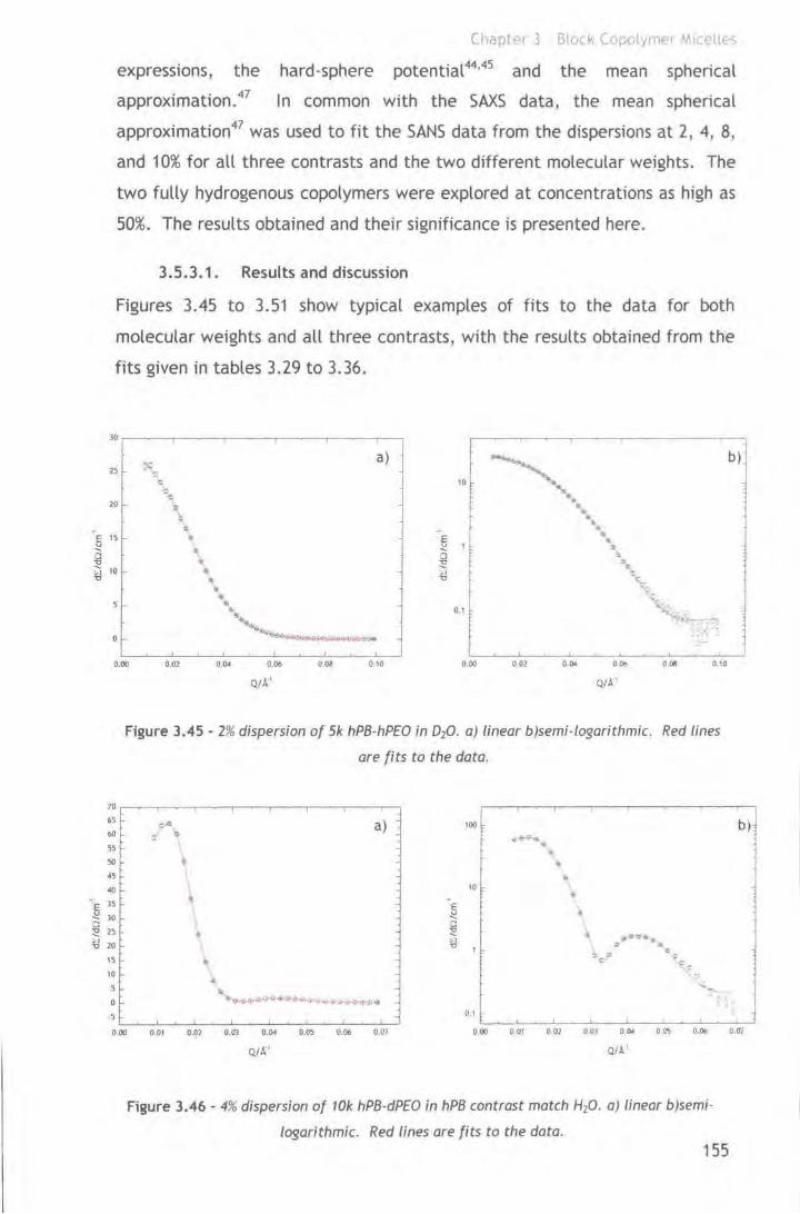
"e ~ c ~
'"'' ~
C'-lar·E>r 3 Block Copolvlll(·J Mlcdles
expressions, the hard-sphere potential44•45 and the mean spherical
approximation. 47 In common with the SAXS data, the mean spherical
approximation47 was used to fit the SANS data from the dispersions at 2, 4, 8,
and 10% for all three contrasts and the two different molecular weights. The
two fully hydrogenous copolymers were explored at concentrations as high as
50%. The results obtained and their significance is presented here.
3.5.3.1. Results and discussion
Figures 3.45 to 3.51 show typical examples of fits to the data for both
molecular weights and all three contrasts, with the results obtained from the
fits given in tables 3.29 to 3.36.
a) b)
20
•
10
E u 1
~ ... ~
0.1
0.00 004 0,06
QtA'
008 0.10 0 .00 0.02 004 O.Ob 008 0.10
70
65
00
55
50
45
40
35
JO
15
20
IS
10
5
0
·5
QtA'
Figure 3.45 - 2% dispersion of 51< hPB-hP£0 in 020. a) linear b)semi-logarithmic. Red lines
are fits to the data.
~· a) 100 -:> 0
\ -~. ~ • ..
• 10
• E ~ • '0 , ~ • ~ .. •e••.,. ~
~:-.: 0
& ~: .. c.
- . -···-10 ...,a.-4wC.<d>~.l""""'•-"v~..-•e ... .
0 .1
0.00 0.01 0.~2 0.0) 0.04 0.05 0.06 0.07 000 0.01 002 0 Ol O.Ool Olr.> 0.06
QIA' Qt!.. '
Figure 3.46 - 4% dispersion of 101< hPB-dP£0 in hPB contrast match H20. a) linear b)semi·
logarithmic. Red lines are fits to the data. 155
b1
0.07

1.8
I 0
... 1.2
.Q 1.0
~ 0.8
~· "0 0.6
0.4
0.2
0.0
Chapter· 3 Block Copolymer ,wceltes
b )
./. '
0.1
0.01 0.02 0.03 O.C).t 0 OS 0.06 0.07 0 08 0.01 0.02 0.03 0 C).t 0.0'5 0 06 0 07 0 08
60
~
20
10
0.00
]~
300
2~
~E 200 V
~ ·~ ~ 100
~
0
Q/A1 QIA''
Figure 3.47- 10% dispersion of 5k dPB-hPEO in hPEO contrast match H20 . a) linear b)semi
logarithmic. Red lines are fits to the data.
0
0.02 o.a.
\ ..
0.06
QIA'
a)
10
0.08 000 0.02 00.
. ~ .. ..
•
006
QIA '
• •
b)
008 0 tO
Figure 3.48 - 20% dispersion of 5k hPB-hPEO in 020. a) linear b)semi-/ogarithmic. Red lines
are fits to the data.
I .. f'
... ;:;;;.f'
a)
.. 111;.)0 ' ..... ~.,. ................................. _. .... ,....,~--.......... -~ ... ..
QIA''
100
o.oo
b)
•
0.02 0 .0< 006 008 0.10
QIA'
Figure 3.49 - 30% dispersion of 10k hPB-hPEO in 020 . a) linear b)semi-logarithmic. Red lines
are fits to the data.
156

~E ~ c ~ ~
100
80
60
40
20
0
.. if ..
• 0~ ... •
0.00 0.02 0.04
a)
.. .. ~
~'*-t ,_ ......_...._,.~~..ih~
0.06 0.03 0. 10
100
Chapter 3 Block Copolymer MICelles
0.00 0.02 0.04
':. .. ~ • • ..
§
"
b)
..
0.06
QtA'
. .. .. .. .. 'l> •o <:~ ~
0.03 010
Figure 3.50- 40% dispersion of 5k hPB·hPEO in 020. a) linear b)semi-logarithmic. Red lines
are fits to the data.
a) b)
200 100
'" 100 10
0
0.00 0.02 0.04 0.06
QIA '
0.03 0.10 0.00 0.02 0.04 006 ooe 0.10
Figure 3.51 -50% dispersion of 10k hPB-hPEO in 020. a) linear b)semi-logarithmic. Red lines
are fits to the data.
157

Chapter 3 - Block Copolymer Micelles
Parameter 10% 8% 4% 2%
Re/A 19 19 20 21
Rs/A 48 48 48 50
~ 0.537 0.548 0.570 0.524
<l>w 0.50 0.55 0.60 0.65
p 27 23 23 20
DPEo/ A 14.39 14.75 14.75 15.13
Rs:Rg 2.06 2.06 2.06 2.15
H-P S(Q) R/A 66.85 63.92 55.08 60.85
Charge 12.84 12.18 9.90 14.48
KIA"1 3.732x10"3 6.526x10"3 1.129x10"2 2.752x10"2
y 9.293 9.504 8.367 48.987
yexp(-k) 5.642 4.130 2.407 1.721
Table 3.29- Parameters from fits to Sk hPB-hPEO in D20 2%scs10%
As for the dilute dispersions, the distinct steps in <1>w result from the model
applied rather than being a real phenomenon of the system, with different
values of this being investigated at each concentration until one providing a
suitable fit was found.
158

Chapter 3 - Block Copolymer Micelles
Parameter 50% . 40% 30% 20%
Re/A 19 17 24 24
Rs/A 32 46 36 37
1R 0.351 o.3n 0.292 0.393
<j)w 0 0 0 0
p 20 14 40 40
OpEQ/ A 15.13 16.00 13.46 13.46
Rs:Rg 1.37 1.97 1.55 1.59
H-P S(Q) RIA 81.09 85.72 n.76 76.81
Charge 40.n 11 8.69 7.87
KIA" 1 5.792x10"2 5.386x10"4 7.21 x10"4 9.117x10"4
y 27061.997 5.054 3.485 2.891
yexp(-k) 2.256 4.573 3.116 2.513
Table 3.30- Parameters from fits to 5k hPB-hP£0 in D20 20%s:cs50%
A point to note about the water volume fraction in table 3.30. Using values
greater than zero resulted in fits of quite poor quality, in terms of both the
parameters and the match to the data. So although the value of 0 is an
unrealistic one, it is the only way a meaningful fit could be generated using
the model applied to the other systems. lt clearly demonstrates the
limitations of the model with respect to higher concentration dispersions.
159
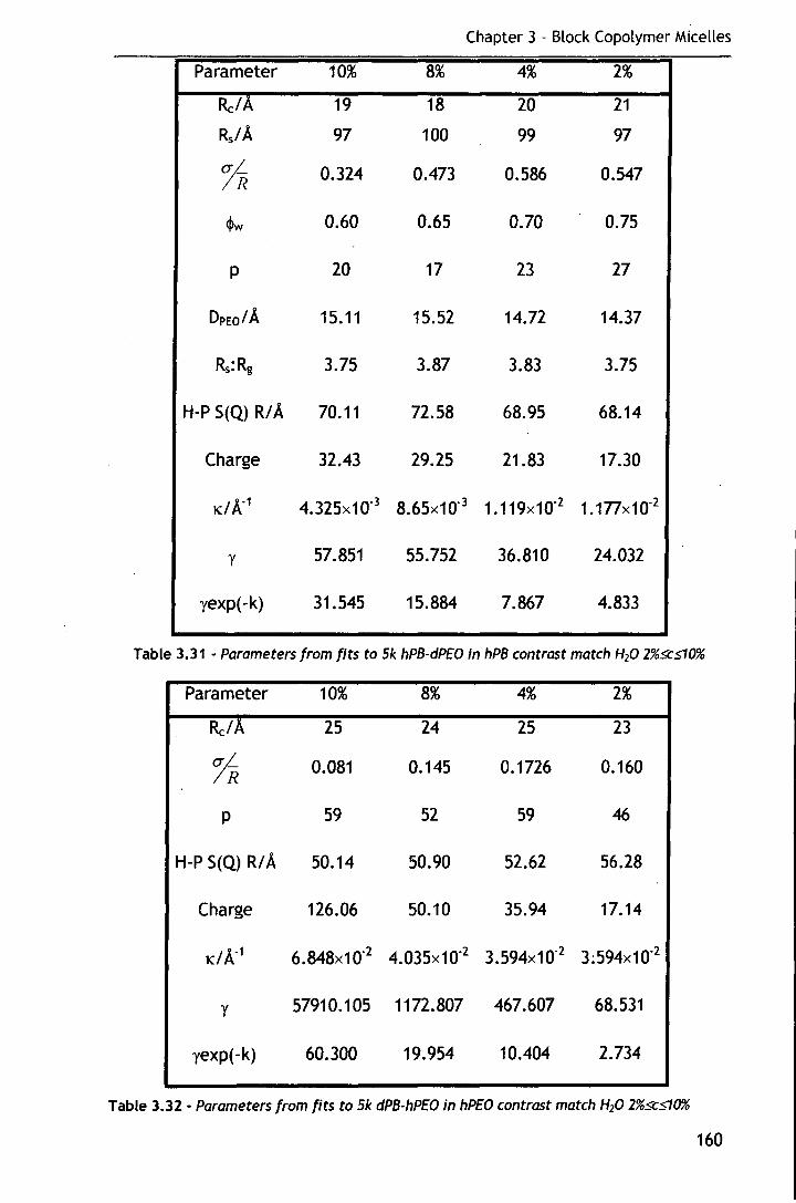
Chapter 3 - Block Copolymer Micelles
Parameter 10% 8% 4% 2%
Re/A 19 18 20 21
Rs/A 97 100 99 97
1R 0.324 0.473 0.586 0.547
<l>w 0.60 0.65 0.70 0.75
p 20 17 23 27
DpEQ/ A 15.11 15.52 14.72 14.37
Rs:Rg 3.75 3.87 3.83 3.75
H-P S(Q) RIA 70.11 72.58 68.95 68.14
Charge 32.43 29.25 21.83 17.30
KIA"1 4.325x10.3 8.65x10"3 1.119x10"2 1.1nx10·2
y 57.851 55.752 36.810 24.032
yexp(-k) 31.545 15.884 7.867 4.833
Table 3.31 -Parameters from fits to Sk hPB·dPEO in hPB contrast match H20 2%5est0%
Parameter 10% 8% 4% 2%
Re/A 25 24 25 23
1R 0.081 0.145 0.1726 0.160
p 59 52 59 46
H-P S(Q) R/A 50.14 50.90 52.62 56.28
Charge 126.06 50.10 35.94 17.14
KIA"1 6.848x10"2 4.035x10"2 3.594x10.2 3:594x10"2
y 57910.105 1172.807 467.607 68.531
yexp(-k) 60.300 19.954 10.404 2.734
Table 3.32 - Parameters from fits to Sk dPB-hPEO in hPEO contrast match H20 2%scst0%
160

Chapter 3 - Block Copolymer Micelles
Parameter 10% 8% 4% 2%
Re/A 40 39 39 39
Rs/A 67 68 71 76
1R 0.489 0.540 0.495 0.505
<Pw 0.5 0.55 0.60 0.65
p 106 98 98 98
DPEo/ A 13.78 13.96 13.96 13.96
Rs:Rg 1.85 1.88 1.96 2.10
H-P S(Q) RIA 110.59 106.20 94.34 82.95
Charge 27.35 25.81 22.56 19.04
K! A"1 2.267x10"3 3.316x10"3 6.413x10"3 1.153x10"2
y 25.505 24.m 25.080 27.616
yexp(-k) 15.449 12.248 7.480 4.078
Table 3.33 - Parameters from fits to 10k hPB-hP£0 in 020 2%SC510%
161

Chapter 3 - Block Copolymer Micelles
Parameter 50% 40% 30% 20%
Re/A 58 63 41 40
Rs/A 13 14 54 51
1R o.1n 0.138 0.10 0.255
~ 0 0 0 0
p 323 414 114 106
DpEQ/ A 11.44 10.98 13.61 13.78
Rs:Rg 0.36 0.39 1.49 1.41
H-P S(Q) R/A ~ 131.72 128.10 124.55 .121.62
Charge 40.n 43.41 120.08 16.85
KIA" 1 2.000x10"2 2.000x10"2 4.439x10"2 1.503x10"3
y 662.463 695.843 614728.672 8.528
yexp(-k) 3.411 4.142 9.702 5.905
Table 3.34- Parameters from fits to 10k hPB-hPEO in D20 20%..<t.s50%
162
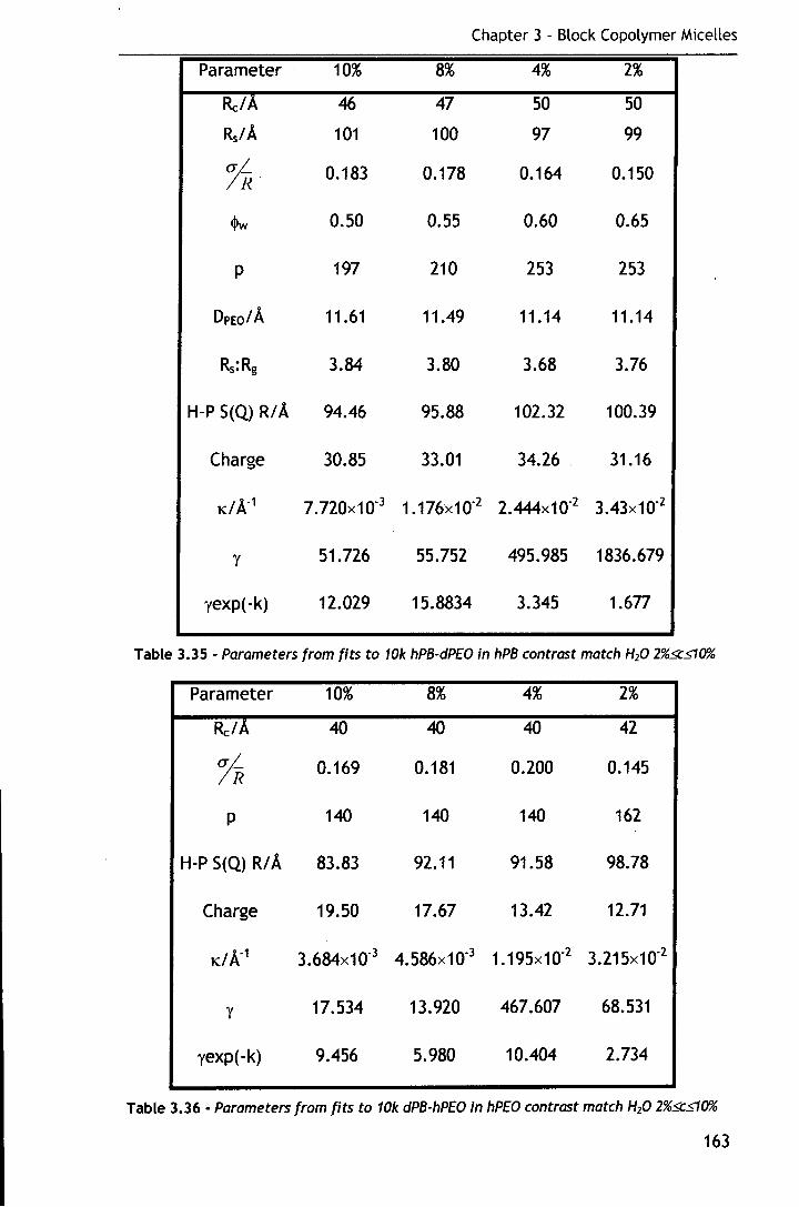
Chapter 3 - Block Copolymer Micelles
Parameter · 10% 8% 4% 2%
Re/A 46 47 50 50
Rs/A 101 100 97 99
~ R. 0.183 0.178 0.164 0.150
<Pw 0.50 0.55 0.60 0.65
p 197 210 253 253
DpEQ/ A 11.61 11.49 11.14 11.14
Rs:Rg 3.84 3.80 3.68 3.76
H-P S(Q) R/A 94.46 95.88 102.32 100.39
Charge 30.85 33.01 34.26 . 31.16
KIA"1 7.720x10"3 1.176x10"2 2.444x10"2 3.43x10"2
y 51.726 55.752 495.985 1836.679
yexp(-k) 12.029 15.8834 3.345 1.6n
Table 3.35- Parameters from fits to 10k hPB-dP£0 in hPB contrast match HzO 2%5tst0%
Parameter 10% 8% 4% 2%
Re/A 40 40 40 42
1R 0.169 0.181 0.200 0.145
p 140 140 140 162
H-P S(Q) R/A 83.83 92.11 91.58 98.78
Charge 19.50 17.67 13.42 12.71
KIA"1 3.684x10"3 4.586x10"3 1.195x10"2 3.215x10"2
y 17.534 13.920 467.607 68.531
yexp(-k) 9.456 5.980 10.404 2.734
Table 3.36 ·Parameters from fits to 10k dPB-hP£0 in hP£0 contrast match H20 2%5tS10%
163
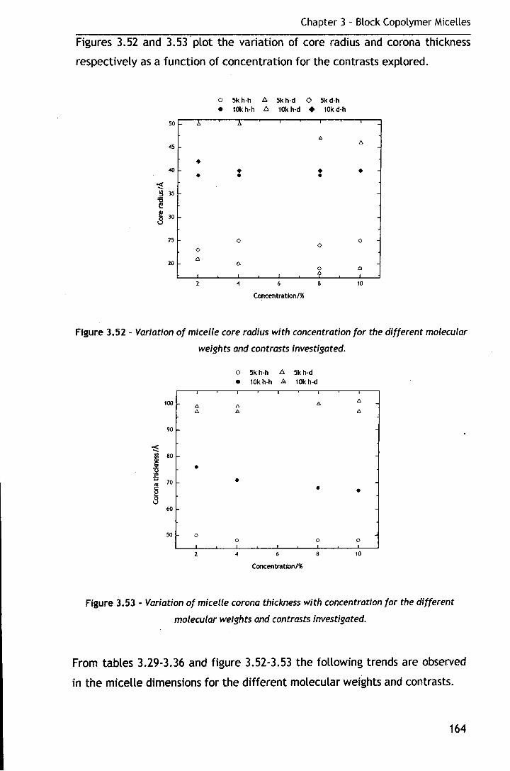
Chapter 3 - Block Copolymer Micelles
Figures 3.52 and 3.53 ·plot the variation of core radius and corona thickness
respectively as a function of concentration for the contrasts explored.
0 5kh-h 6. 5kh-d <> 5kd-h
• 10k h-h !::. 10kh-d • 10k d-h
50 2;. 2;.
A
45
• 40 • • • • • •
~ ~ 35
~ ~30
25 <> 0 <>
0
20 a
6
~ a
4 6 8 10
Corcentration/%
Figure 3.52- Variation of micelle core radius with concentration for the different molecular
weights and contrasts investigated.
100 A A
90
~
j 80
• u :E ...
70
~ u 60
50 0
2
0 5k h-h 6. 5k h-d e 10kh-h A 10kh-d
•
0
4 6
Concentration/%
•
0
8
•
0
10
Figure 3.53- Variation of micelle corona thickness with concentration for the different
molecular weights and contrasts investigated.
From tables 3.29-3.36 and figure 3.52-3.53 the following trends are observed
in the micelle dimensions for the different molecular weights and contrasts.
164
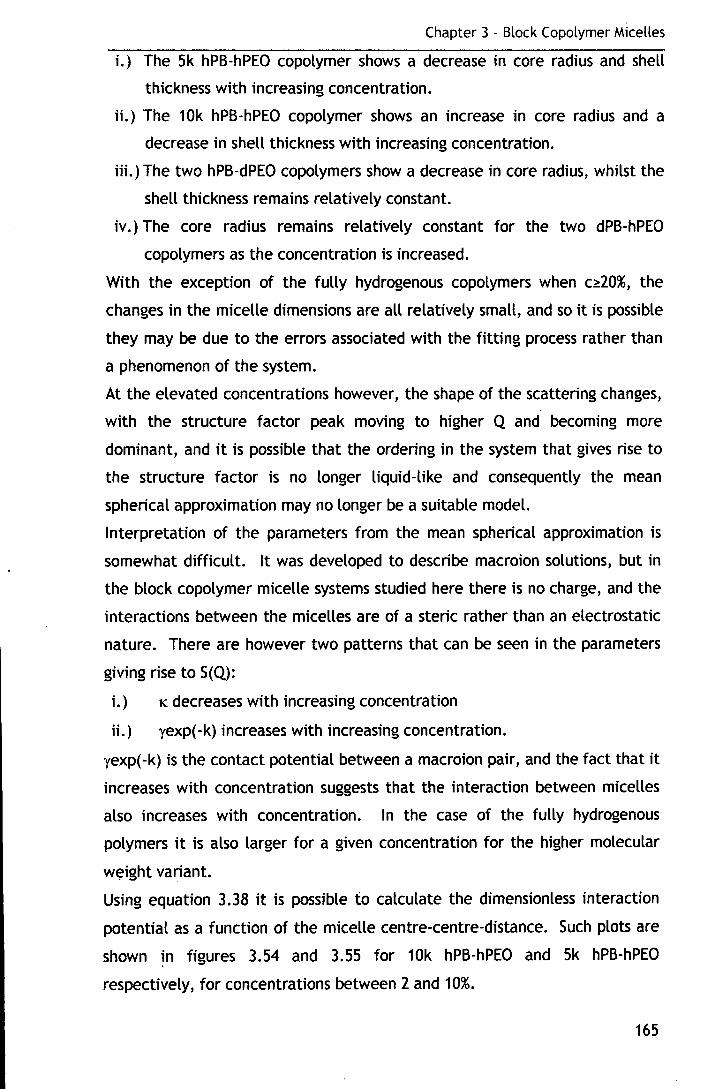
I •
Chapter 3 - Block Copolymer Micelles
i.) The 5k hPB-hPEO copolymer shows a decrease in core radius and shell
thickness with increasing concentration.
ii.) The 1 Ok hPB-hPEO copolymer shows an increase in core radius and a
decrease in shell thickness with increasing concentration.
iii.) The two hPB-dPEO copolymers show a decrease in core radius, whilst the
shell thickness remains relatively constant.
iv.) The core radius remains relatively constant for the two dPB-hPEO
copolymers as the concentration is increased.
With the exception of the fully hydrogenous copolymers when c~20%, the
changes in the micelle dimensions are all relatively small, and so it is possible
they may be due to the errors associated with the fitting process rather than
a phenomenon of the system.
At the elevated concentrations however, the shape of the scattering changes,
with the structure factor peak moving to higher Q and becoming more
dominant, and it is possible that the ordering in the system that gives rise to
the structure factor is no longer liquid-like and consequently the mean
spherical approximation may no longer be a suitable model.
Interpretation of the parameters from the mean spherical approximation is
somewhat difficult. lt was developed to describe macroion solutions, but in
the block copolymer micelle systems studied here there is no charge, and the
interactions between the micelles are of a steric rather than an electrostatic
nature. There are however two patterns that can be seen in the parameters
giving rise to S(Q):
i.) K decreases with increasing concentration
ii.) yexp( -k) increases with increasing concentration.
yexp( -k) is the contact potential between a macroion pair, and the fact that it
increases with concentration suggests that the interaction between micelles
also increases with concentration. In the case of the fully hydrogenous
polymers it is also larger for a given concentration for the higher molecular
w~ight variant.
Using equation 3.38 it is possible to calculate the dimensionless interaction
potential as a function of the micelle centre-centre-distance. Such plots are
shown ~n figures 3.54 and 3.55 for 10k hPB-hPEO and 5k hPB-hPEO
respectively, for concentrations between 2 and 10%.
165
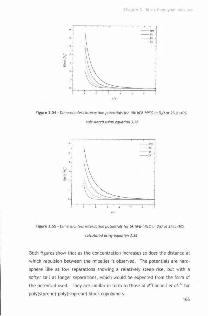
14
12
10
0
rltr
Chapter :: Block Copolymer Mrcel.~
-- 11». --8%
4% -- 2't
6
Figure 3.54- Dimensionless interaction potentials for 10k hPB-hPEO in 0 20 at l %5c510%
6
5
0
0
calculated using equation 3.38
r/cr
--10% --8'\,
4~
--2\
6
Figure 3.55- Dimensionless interaction potentials for Sk hPB-hPEO In 020 at 2%5<:<10%
calculated using equation 3.38
Both figures show that as the concentration increases so does the distance at
which repulsion between the micelles is observed. The potentials are hard
sphere like at low separations showing a relatively steep rise, but with a
softer tail at longer separations, which would be expected from the form of
the potential used. They are similar in form to those of M' Connell et al. 62 for
poly(styrene )-poly( isoprene) block copolymers. 166

Chapter 3 Block Copolyp1Pf MICelles
Figure 3.56 and 3.57 show the dimensionless interaction potentials for the two
hPB-hPEO polymers at concentrations between 20 and 50%.
10 --20'li 9 --30'li
--50% 7
0
r/a
Figure 3.56 - Oimensionless interaction potentials for 10k hPB-hPEO in 020 at 20%.5ts50%
calculated using equation 3.38
5.0
4.5
\ 4.0
3. 5
--20%
--JO'li
--50\1;
3.0
1-.>/!.ID 2.5 --~ 2.0
5 1.5
1.0
0.5
0.0
0 4 6 10 11
r/a
Figure 3.57 • Oimensionless interaction potentials for 51< hPB-hPEO in 0 20 at 20%.5ts50%
calculated using equation 3.38
Figure 3.56 suggests that at concentrations greater than 20% the micelles
behave as hard spheres. Figure 3.57 shows that at concentrations between 20
and 40% inclusive the micelles still interact with one another at distances up
167
Chapter 3 - Block Copolymer Micelles
to ten times their diameter; whilst above this they behave as hard spheres.
The validity of these observations is open to question since the mean
spherical approximation does not reproduce entirely all of the features of the
data at these elevated concentrations. Indeed at the higher end of these
values the dispersions no longer flow and are solid intractable gels, where
different physical principles govern the micellar interactions compared to
more dilute liquid~like dispersions.
In an approach applied by Bown et al. 54 it is possible to calculate reduced
force-distance profiles for the fully hydrogenous polymers from the
interaction potentials using the relationships of Patel et al. 63 (equations 3.50-
3.52).
force I= ((T(2v+l)/2v allv N) Equation 3.51
where fis reduced force, cr is the grafting density, a is the segment length, v
is the excluded volume parameter, N is the degree of polymerisation of the
corona forming block.
Equation 3.52
where 8 is the reduced distance.
F(r I D)= trRcU(r I D) Equation 3.53
168

Chapte1 3 Block. Copolymer MJceUE~c;
--I
10 --4~
--2%
Ill
] 0.1
~ ~ 0.01
1E·l
lE·~+---.,.------.------,,.........,.--,-..,..........,........----.--..---.--~
1!·3 0.01
Reduced distance
Figure 3.58- Reduced force as a function of reduced separation of micelle cores for 5k hPB
hPEO
100
10
0 .01
1E·J
1E· l
Reduced distance
-- 100:. 8'\i
--4~
--2%
0 01
Figure 3.59- Reduced force as a function of reduced separation of micelle cores for 10k
hPB-hPEO
The potent1als 1n figures 3.58 and 3.59 are comparable to those obtained by
Bown et al. 54 and Patel et al. 63 with the former attribut1ng the shape as being
due to the corona behaving as a brush-like layer.
169

Chapter 3 - Block Copolymer Micelles
3.5.3. Conclusions
As with the previous sections, the main conclusions that can be inferred from
the data are summarised here for clarity.
• The block copolymers investigated form micelles when dispersed in water
that are spherical in nature.
• The average dimensions of the micelles have been determined by fitting
the data to a spherical core-shell model with a parabolic volume fraction
profile in the shell.
• The lower molecular weight micelles have core radii of ea 22A and a shell
thickness of ea BOA. · ·
• The higher molecular weight micelles have core radii of ea 40A and a
shell thickness of ea 11 OA. • The PEO chains composing the corona are highly stretched compared to
the unperturbed radius of gyration, and the separation distance between
them is less than the radius of gyration allowing them to be considered as
a polymer brush.
• Reasonable agreement with predicted brush heights and experimentally
determined corona thicknesses was observed, with the relationship of Dan
and Tirrell61 providing the best agreement.
• Micelles formed by the two molecular weight series have quite different
association behaviour, with the lower molecular weight micelles having
modest association numbers whereas the higher molecular weight
micelles have high association numbers.
• Reasonable agreement was found between the experimental data and the
scaling relations of Halperin's star model. 29
• A structure factor due to intermicellar interactions is evident as the
concentration is increased, and this has been successfully modelled using
the mean spherical approximation.
• As the concentration is increased still further, the shape of the scattering
changes suggesting that the type of ordering is changing from liquid-like
to solid-like.
170
Chapter 3 - Block Copolymer Micelles
3.6. Final discussion
The poly(butadiene)-poly(ethylene oxide) block copolymers investigated here
formed spherical micelles in aqueous solution with low erne's that were seen
to be inversely related to the molecular weight of the copolymer.
Comparison of these erne's with those of other PEO containing diblock
copolymers reported in the literature suggests that the hydrophobic character
of PB lies somewhere between that of poly(butylene oxide) and
poly( propylene oxide) with the later being the least hydrophobic. Calculation
of hydrophile-lipophile balance for the three respective hydrophobes suggests
the PB and PBO have approximately equivalent hydrophobic character, whilst
PPO is the most hydrophilic of the three. Deng et al.64 suggested that PB was
more hydrophobic than PBO, although offered no evidence to support this
claim. Elucidation of the hydrophobic character of PB in PB-PEO block
copolymers is complicated by the small data set existing for such species, and
so the conclusions drawn here can only serve as indicative observations rather
than quantitative answers.
In common with reports for other block copolymers, PB-PEO appears to
undergo micellisation by the closed association process, forming micelles
having narrow size distributions as determined by CONTIN analysis of QELS
data. The concentration dependence of the apparent diffusion coefficient
allowed the elucidation of the micelle hydrodynamic radii, with values of
168A and 136A determined for the 10k and the 5k micelles respectively. The
two molecular weights exhibited different concentration dependencies of the
for the diffusion coefficient, with the lower molecular weight variant
displaying the usual positive dependence due to repulsive interactions
between micelles expected for diblock copolymers. The higher molecular
weight micelles showed a negative dependence more commonly associated
with triblock copolymers due to attractive interactions between micelles.
The reason for the latter observation remains unclear since the synthetic
procedure precludes the formation of triblock copolymers and SEC analysis of
the block copolymer showed a monomodal distribution suggesting that no
homo PEO was formed during the polymerisation reaction. One can only
speculate as to the reasons for this unusual observation, with perhaps the
171

Chapter 3 - Block Copolymer Micelles
presence of some impurity not detected by SEC or NMR, or indeed from the
water used to prepare the samples has caused this tendency.
Comparison of the hydrodynamic radii determined from QELS experiments on
other PEO containing block copolymers (table 3.4) reveal that for those
copolymers having similar compositions and molecular weights to the two
studied here, reasonable agreement between the radii is observed. This
result is not unexpected since the copolymers considered formed spherical
micelles due to PEO being the major constituent. Under such circumstances,
the corona would be expected to be the largest part of the micelle since the
PEO chains are in a good solvent, and as the nature of the corona forming
chains is the same in all of the species reasonable agreement could be
expected.
The determination of the micelle radii from the fitting of SANS data due to
dilute dispersions concurred fairly well with the hydrodynamic radii from the
QELS experiments, with the latter values being slightly larger. The model
used to fit the SANS data also allowed determination of the core radius of the
micelles, with a value of 19-25A observed for the Sk series and 35-45A for the
1 Ok series. Interestingly these values are considerably smaller than those
determined by Bates and eo-workers using cryo-TEM65 and SANS66 for PB-PEO
block copolymers having comparable molecular weights and compositions to
those investigated here. Cryo-TEM experiments suggested a core radius of
150A and a shell thickness of 330A for an 8k copolymer containing 70% PEO, 65
whilst fits to SANS data suggested a core radius of 111A and a shell thickness
of 178A for a similar copolymer. 66 The fact that the core radii are larger than
determined here could be attributed to the larger PB block, but as the PEO
block length of the two copolymers studied by Bates and eo-workers are
shorter than those examined here, one would expect the corona thickness to
be less than that determined here. The increased dimensions from the TEM
experiments may result from the vitrification procedure used to prepare the
films of the micelles for examination. The micelles could potentially "spread
out" on the grid used, a phenomenon observed by Wooley and eo-workers, 67
resulting in increased dimensions. The differences from the SANS experiments
are likely to result from the different models used to fit the data. Won et 171
Chapter 3 - Block Copolymer Micelles
al. 66 used a Fermi-Dirac function to model the density profile of the corona as
opposed to the parabolic function employed here.
Determination of micelle dimensions from SLS proved troublesome due to the
poor quality of the data, with Zimm plot analysis suggesting the Sk micelles
had a larger radius of gyration than their 1 Ok counterparts; an observation
that is clearly erroneous. The shape of the Zimm plot for the Sk micelles
showed the extrapolated data "hooking back up" from the lowest
concentration. This may be due to experimental error in the preparation of
one or more of the dispersions, although there is some evidence of similar
phenomena in the literature. 38 The intensity of the laser utilised could also be
a problem, with the power output measured as 53 mW, resulting in quite a
weak scattering intensity
Modelling of SAXS data to give micelle dimensions was hampered by the weak
scattering intensity and the lack of SAXS contrast between the three
scattering components in the system. lt was not possible to measure
scattering at concentrations below 1%, and even at this concentration, the
scattering from the dispersions was weak in intensity. The results obtained
from fitting Sk hPB-hPEO were particularly unrealistic, with the model
suggesting a core radius of 60A and a shell thickness of 12A, clearly out of
proportion with the copolymer composition. Fits to the 10k data were a little
more successful, revealing a core radius of ea 14A and a shell thickness of
40A, both smaller than the values obtained by SANS. With hindsight, it would
have been better to perform the SAXS experiments using a synchotron source,
which would have provided a far greater incident flux, and removed the need
for desmearing, which can add complications to the data.
The association number of the micelles, p, could be calculated from the core
radii determined from fits to the SANS data based upon the molecular weight
and density of PB block forming the core. The two molecular weight series
exhibited contrasting association behaviours, with the Sk series showing
moderate association numbers of 20-45 and the 1 Ok series exhibiting high
association numbers of 70-230. Won et al.66 used a similar method for their
spherical PB-PEO micelles discussed above and determined an association
173
Chapter 3 - Block Copolymer Micelles
number of 1350, which is considerably larger than the values obtained here,
and of other PEO based block copolymers reported in the literature. They
attributed the large association number compared to PPO-PEO copolymers to
the strongly hydrophobic nature of the PB core reducing the number particles
in the system in order to minimise the unfavourable contact with water.
Several authors including Mortensen et al. 5 and Bown et al. 54 have employed
the same method for determining association numbers and obtained
conflicting results, with the former reporting p=470 for a 4k PS-PEO block
copolymer and the latter reporting ea 135 for an 8k PS-PEO. These two values
are considerably smaller than that determined by Won et al66• and on
polymers that are more hydrophobic than PB-PEO, so their result and
explanation for it appear questionable.
Booth and eo-workers have reported association numbers for PBO-PEO block
copolymers determined by SLS, 2• 3 suggesting a similar pattern to that
observed here; namely low to moderate values for lower molecular weight
species increasing to higher values with molecular weight. They noted that
the length of the hydrophobic block was the primary determinant of the
association number, with the two being proportionally related. The length of
the hydrophilic block was seen to exert less influence with a small increase in
its length resulting in a small decrease of the association number. Given the
limited data set available for PB-PEO block copolymers (these results and
those of Won et al. 66) one could speculate that the association numbers
observed support the observations of Booth and eo-workers previously stated.
Attempts to determine the association numbers from SLS data proved fruitless
due to the poor quality of the data.
From the association number, the separation distance between PEO chains on
the surface of the micelle core could be calculated. These distances were
compared to the unperturbed radii of gyration of the corona-forming PEO
chain in water calculated using the relationship of Kawaguchi et al. 56 In all
instances the separation distance was less than the radius of gyration.
Comparison of the corona thickness to the same radius of gyration revealed
that the chains forming the corona were highly stretched, (2.5-4.5x), relative
to the unperturbed state. These two observations supported the notion of 174
Chapter 3 - Block Copolymer Micelles
considering the coronal layer as a polymer brush, which was applied during
the fitting procedure in terms of the polymer volume fraction profile.
Comparison of the experimentally determined brush heights to the theoretical
models of Alexender, 59 de Gennes, 60 Milner et al55• and Dan and Tirrell61
revealed that the latter of these provided the closest agreement. This was
not surprising since the others were postulated for planar surfaces whilst the
Dan and Tirrell61 model was formulated for curved interfaces.
As the concentration was increased above 1% the size distributions observed
by QELS were seen to change markedly; first a broadening effect, then a
bimodal population was observed. The two molecular weights again showed
contrasting behaviour, with the 10k polymer exhibiting bimodal populations at
c?:8%, with the smaller particles having a radius of 11 OA and the larger ones ea
3 times. that. The 5k micelles on the other hand showed bimodal populations
at c?:4%, with the smaller particles having radii of 110A and the larger ones 6-
10 times that. The larger particles in both instances are likely micelle
clusters similar to those reported by Xu et af. for PS-PEO in water. They
observed that the dimensions of these micellar aggregates were of the order
of 10 times greater than the micelles. In future in may be beneficial to be
able to fit the SANS data to a model accounting for the dual populations
observed from the QELS experiments. This is currently not possible using the
model and the software applied here.
The 10k copolymer behaviour is a little unusual since the dimensions of the
larger particles are not as large as those of the 5k micelles or similar
examples reported in the literature. 7 This may result from the clusters being
more tightly bound due to the attractive nature of the interactions between
the micelles suggested by the concentration dependence of the diffusion
coefficient. As the clusters were not always observed it is possible they are
non-equilibrium structures or due to impurities in the dispersion causing
temporary micelle bridging, which would explain the negative concentration
dependence of the diffusion coefficient.
The SAXS intensity from dispersion where c?:2% was much greater than those
from the 1% dispersions for both molecular weights. At these higher
concentrations a structure factor peak due to intermicellar interactions was 175
Chapter 3 - Block Copolymer Micelles
clearly evident and so account had to be taken of this when fitting the data.
Initial attempts at using a hard-sphere potential were unsuccessful, with it
not adequately describing the structure observed in even the most dilute of
these dispersions.
The use of the mean spherical approximation resulted in fits that reproduced
most of the features of the data, although it did not quite capture all of
them. As for the dilute dispersions the lack of contrast made it difficult to
obtain accurate micelle dimensions, with the 10k micelles giving a core radius
of 13A and a shell thickness of 50A, whilst the 5k micelles gave a core radius
of 6A and a shell thickness of 30A. All of these values are smaller than those
determined by fits to the SANS data where the degree of contrast is greatly
enhanced. The intermicellar interactions could not be determined
quantitatively since the fits did not accurately reproduce the data.
There are few reports of SAXS investigations on micellar dispersions in the
literature, with most investigations focusing on higher concentration
mesophases or solid samples.24'
64'
68 Presumably, this is due to the lack of
contrast experienced here.
Fits to the SANS data for higher concentration dispersions proved far more
successful than those from the SAXS data, with the mean spherical
approximation accurately reproducing the features observed in the scattering
data for samples where the dispersion was still liquid-like rather than a gel.
Consequently, it was possible to obtain a more complete picture of the
. intermicellar interactions.
As discussed in section 3.5.3.1 there were small changes in the micelle
dimensions for those dispersions at c::;10%. Whether these changes in
dimensions were a result of the errors associated with the fitting process or a
genuine phenomenon of the system remains unclear.
The degree of stretching, determined by Rs: Rg , was seen to decrease with
increasing concentration, presumably due to the micelles coming closer
together and causing the coronal chains to contract slightly.
At the lowest concentration the interaction between the micelles is close to
that of a hard-sphere potential, with a steep rise in the potential energy at
short separation distances, and a relatively short tail. As the concentration 176

Chapter 3 - Block Copolymer Micelles
increases, the rises in the potential energy at low separation become less
dramatic and the tail longer and softer, with interactions between micelles
evident at greater degrees of separation. Other researchers have reported
similar potentials including McConnell et al62• whose potentials were
calculated from self-consistent field theory.
Interpretation of the potentials at higher concentrations is complicated by the
model not fully reproducing the features of the data. However, it appears
that when the dispersions are still liquids the same pattern discussed above is
observed, namely an increasingly softer tail and interactions at longer
distances are observed. When the dispersions form gels the potential reverts
to that approaching a hard sphere, with steep rises in the potential at low
separations and little interaction at longer distances.
3.7. Glossary of symbols
The symbols used in the body of the text and the equations are defined here
in the order in which they appear in the text.
3. 7.1. Introduction
Q scattering vector
n refractive index
'A wavelength
8 scattering angle
Rg radius of gyration
Mw weight average molecular weight
A2 second virial coefficient
p association number
D diffusion coefficient
Rh hydrodynamic radius
3.7.2. Quasi-Elastic Light Scattering
Dapp
ks
T
apparent diffusion coefficient
Boltmann constant
temperature

R
K
erne
Do
c
kt
V
Chapter 3 - Block Copolymer Micelles
solvent viscosity
apparent hydrodynamic radius
Gibbs energy of association
Universal gas constant
micelle association constant
critical micelle concentration
diffusion coefficient at infinite dilute
diffusion second virial coefficient
concentration
frictional coefficient
partial specific volume of micelles in solution
micelle radius
degree of polymerisation of core forming B block
. degree of polymerisation of corona forming A block
segment length
3. 7.3. Static Light Scattering
w weight fraction of component in copolymer
MA molecular weight of A block
MB molecular weight of B block
MnA number average molecular weight of A block
Mn6 number average molecular weight of B block
Mn number average molecular weight of copolymer
MwA weight average molecular weight of A block
Mw6 weight average molecular weight of B block
Mw weight average molecular weight of copolymer
R-Ro excess Rayleigh ratio
K optical constant
M molecular weight
d% de specific refractive index increment
P(e) particle scattering factor
no solvent refractive index
NA Avogadro's number
178
"/.
A.o
M
(d%ct (d%JB Mw,app
p
3.7.4.
I(Q)
N
V
Q
R
(.1p )2
Rg
Pc
Ps
Pm
R
cr
z r(Z+l)
Chapter 3 - Block Copolymer Micelles
incident wavelength
average molecular weight
apparent molecular weight
weight fraction of A in copolymer
weight fraction of B in copolymer
specific refractive index increment of A block
specific refractive index increment of B block
weight average apparent molecular weight
micelle association number
polymer refractive index
change in refractive index
Rayleigh ratio at angle e second virial coefficient
radius of gyration
thermodynamic radius
Rayleigh ratio at 90°
Small-angle X-ray scattering
scattering intensity
number of scattering particles
particle volume
scattering vector
radius of a sphere
contrast (electron density difference)
radius of gyration
electron density of micelle core
electron density of micelle corona·
electron density of solvent
average core radius
standard deviation of Schultz distribution
width parameter of Schultz distribution
gamma function
179
( l
11
V
U(r)
0'
\jJO
K
Zm
n
separation distance
hard sphere radius
Chapter 3 - Block ~opolymer Micelles
hard sphere volume fraction
total volume of system
repulsion potential between spherical macroions
macroion diameter
permitivity of free space
solvent relative permitivity
surface potential
Debye-Huckel inverse screening length
~lectronic charge
number of particles
3. 7.5. Small-angle neutron scattering
Q
(dL/dQ)(Q)
~Pc
~Pc
<l>w
1R ~PB
~PEO
Rg.
Mw
p
Vps
mps
NA
PPB
NA
Ns
scattering vector
differential scattering cross-section
scattering length density difference between core and
inner most sub-shell of corona
scattering length density difference between innermost
shell of corona and solvent
volume fraction of water in inner most sub-shell of corona
width of Schultz distribution
volume fraction of poly(butadiene)
. volume fraction of poly( ethylene oxide)
radius of gyration
weight average molecular weight
micelle association number
volume of poly(butadiene) block
molecular weight of poly(butadiene) block
Avogadro's number
density of poly(butadiene) block
degree of polymerisation of corona forming A block
degree of polymerisation of corona forming B block 180

V
cr
h
N
cr
R
1(
U(r/cr)
r/cr
f
cr
Chapter 3 - Block Copolymer Micelles
excluded volume parameter
interfacial area per chain
brush height
degree of polymerisation of brush forming polymer
grafting density
radius of curvature (core radius)
Debye-Huckel inverse screening length
dimensionless interaction potential
dimensionless separation
reduced force
reduced distance
D (same as cr for S(Q)) macroion diameter
3.8. Bibliography
2
3
4
5
6
7
8
9
10
11
12
13
14
D. J. Shaw, 'Introduction to Colloid and Surface Chemistry', 4th, ed.,
Butterworth-Heinemann, Oxford, 1998.
C. Booth and D. Attwood, Macromol. Rapid Commun., 2000, 21, 501.
C. Booth, G. E. Yu, and V. M. Nace, in 'Amphiphilic block copolymers:
Self assembly and applications', ed. P. Alexandridis and B. Lindman,
Elsevier, Amsterdam, 2000.
B. Chu and Z. Zhou, in 'Nonionic surfactants: Polyoxyalkylene block
copolymers', ed. V. M. Nace, Marcel Dekker New York, 1996.
K. Mortensen, et al., Langmuir, 1997, 13, 3635.
M. Willhelm, et al., Macromolecules, 1991, 24, 1033.
R. L. Xu, et al., Macromolecules, 1991, 24, 87.
Z. Zhou, B. Chu, and V. M. Nace, Langmuir, 1996, 12, 5016.
T. Liu, et al., J. Phys. Chem. B, 1997, 101, 8808.
L. Derici, et al., Phys. Chem. Chem. Phys., 1999, 1, 2n3.
W. Mingvanish, C. Chaibundit, and C. Booth, Phys. Chem. Chem. Phys.,
2002, 4, n8. P. F. Dewhurst, et al., Macromolecules, 1998, 31, 7851.
S. W. Provencher, Makromol. Chem., 1979, 180, 201.
H. G. Elias, in 'Light Scattering from Polymer Solutions', ed. M. B.
Huglin, Academic Press, London, 1972. 181

15
16
17
18
19
20
21
22
23
24
25
26
27
28
29
30
31
32
33
34
35
36
37
38
39
Chapter 3 - Block Copolymer Micelles
I. W. Hamley, The Physics of Block Copolymers', Oxford University
Press, New York, 1998.
Y.-W. Yang, et al., Langmuir, 1995, 11, 4703.
S. M. Mai, et al., Langmuir, 2000, 16, 1681.
Y. Zheng and H. T. Davis, Langmuir, 2000, 16, 6453.
J. T. Davies and E. K. Rideal, 'Interfacial Phenomena', 2nd, ed.,
Academic Press, New York, 1963.
R. J. Hunter, 'Foundations of Colloid Science Vol 2', Oxford University
Press, New York, 1989.
Z. K. Zhou, et al., Macromolecules, 1996, 29, 8357.
C. Konak, et al., Progr. ColloidPolym. Sci., 1985,71,15.
J. Selser, in 'Dynamic Light Scattering- The method and some
applications', ed. W. Brown, Clarendon Press, Oxford, 1993.
A. Kelarakis, et al., J. Chem. Soc., Faraday Trans., 1998, 94, 3639.
W. Mingvanish, et al., J. Phys. Chem. 8, 1999, 103, 11269.
A. Kelarakis, et al., J. Phys. Chem. 8, 2001, 105, 7384.
Y.-W. Yang, et al., Macromolecules, 1996, 29, 670.
S.-M. Mai, et al., J. Chem. Soc., Faraday Trans., 1998, 94, 567.
A. Halperin, Macromolecules, 1987, 20, 2943.
R. Nagarajan and K. Ganesh, J. Chem. Phys., 1989, 90, 5843.
A. Kelarakis, et al., Phys. Chem. Chem. Phys., 2001, 3, 4037.
R. L. Xu, et al., Macromolecules, 1992, 25, 644.
H. Benoit and D. Froelich, in 'Light Scattering from Polymer Solutions',
ed. M. B. Huglin, Academic Press, London, 1972.
M. B. Huglin, in 'Light Scattering from Polymer Solutions', ed. M. B.
Huglin, Academic Press, London, 1972.
J. Brandup and E. H. lmmergut, 'Polymer Handbook', 3rd, ed., John
Wiley and Sons, Toronto, 1989.
B. L. Johnson and J. Smith, in 'Light Scattering from Polymer Solutions·,
ed. M. B. Huglin, Academic Press, London, 1972.
W. Burchard, M. Schmidt, and W. H. Stockmayer, Macromolecules,
1980, 13, 580.
W. Burchard, in 'Applied Fibre Science', ed. F. Happey, Academic Press,
1978.
E. B. Zhulina and T. M. Birshtein, Polymer Science USSR, 1986, 27, 570.
182
40
41
42
43
44
45
46
47
48
49
50
51
52
53
54
55
56
57
58
59
60
61
62
63
64
65
Chapter 3 - Block Copolymer Micelles
N. F. Carnahan and K. E. Starling, J. Chem. Phys., 1969, 51, 635.
J. S. Pedersen and C. Svaneborg, Curr. Opinion Coil. Interface Sci.,
2002, 7, 158.
V. Castelletto and I. W. Hamley, Curr. Opinion Coil. Interface Sci.,
2002, 7, 167.
R. H. Ottewill, Ch7 in 'Colloidal Dispersions', ed. J. W. Goodwin, Royal
Society of Chemistry, London, 1982.
N. W. Ashcroft and J. Lekner, Phys. Rev, 1966, 145, 83.
J. K. Perkus and G. J. Yevick, Phys. Rev, 1958, 110, 1.
R. H. Ottewill, Ch 9 in 'Coloidal Dispersions', ed. J. W. Goodwin, Royal
Society of Chemistry, London, 1982.
J. B. Hayter and J. Penfold, Molec. Phys., 1981, 42, 109.
I. W. Hamley, et al., Langmuir, 2001, 17,6386.
S. M. King, in 'Modern Techniques of Polymer Characterisation', ed. R.
A. Pethrick and J. V. Dawkins, John Wiley & Sons, London, 1999.
'Small Angle X-ray Scattering', ed. 0. Glatter and 0. Kratky, Academic
Press, 1982.
R. K. Heenan, The "Fish" Reference Manual', RAL-TR-89-129, Rutherford
Appleton Laboratory, Didcot, 2000.
M. Kotlarchyk and S.-H. Chen, J. Chem. Phys., 1983, 79, 2461.
J. S. Higgins, et al., Polymer, 1988, 29, 1968.
G. J. Bown, R. W. Richards, and R. K. Heenan, Polymer, 2001, 42,
7663.
S. T. Milner, T. A. Witten, and M. E. Cates, Macromolecules, 1988, 21,
2610.
S. Kawaguchi, et al., Polymer, 1997, 38, 2885.
K. Taskai, J. Am. Chem. Soc., 1996, 118, 8459.
M. Daoud and J. P. Cotton, J. Physique, 1982, 43, 531.
S. Alexander, J. Physique, 1977, 38, 983.
P. G. de Gennes, J. Physique, 1976, 37, 1445.
N. Dan and M. Tirrell, Macromolecules, 1992, 25, 2890.
G. A. McConnell, et al., Faraday Discuss., 1994, 98, 121.
S. Patel, M. Tirrell, and G. Hadziioannou, Colloids Surf., 1988, 31, 157.
Y. Deng, et al., Polymer, 2002, 43, 7155.
Y. Zheng, et al., J. Phys. Chem. B, 1999, 103, 10331.
183

66
67
68
Chapter 3 - Block Copolymer Micelles
Y. Y. Won, et al., J. Phys. Chem. B, 2000, 104, 7134.
H. Huang, et al., J. Am. Chem. Soc., 1997, 119, 11653.
I. W. Hamley, et al., Langmuk, 2002, 18, 1051.
184
Chapter 4 - Cross-linked micelles
4. Cross-linked micelles
185

Chapter 4 - Cross-linked micelles
4.1. Introduction
Micelles formed from the self-assembly of block copolymers in selective
solvents are non-permanent structures held together by molecular
interactions such as hydrophobic-hydrophilic effects, hydrogen bonding or van
der Waals forces. 1 These interactions are relatively weak, and impart a
reversible nature to the self-assembly process. The physical properties of the
self-assembled structures can be changed by subsequent post self-assembly
manipulation. One such change is to chemically fix or cross-link part of the
micelle having a suitable functional group. This area has received a growing
amount of attention in recent years. 2"17 Chapter one surveyed the major
advances in the field of cross-linked micelles, both of the core and shell
cross-linked variants. The various different methodologies and outcomes
were reviewed and discussed.
This chapter focuses on the core cross-linked micelles produced, and their
properties as determined by the scattering techniques utilised in chapter
three for the study of virgin copolymer micelles. These properties will be
compared to those of the micelles and differences rationalised.
4.2. Cross-linked micelle production
As demonstrated in chapter three, poly(butadiene)-poly(ethylene oxide) block
copolymers readily form micelles when dispersed in water at low
concentrations. The presence of double bonds in the core, should prove
suitable functional groups to cross-link the micelles.
Chapter two provided the synthetic details relating to the cross-linking
procedure and subsequent physical characterisation of the cross-linked
micelles, and the reader is referred to sections 2.3.2 and 2.6.2 for further
details.
The procedures outlined in chapters two and three for the collection and
subsequent treatment of data were as employed for the micelles and so are
not presented in detail here.
186
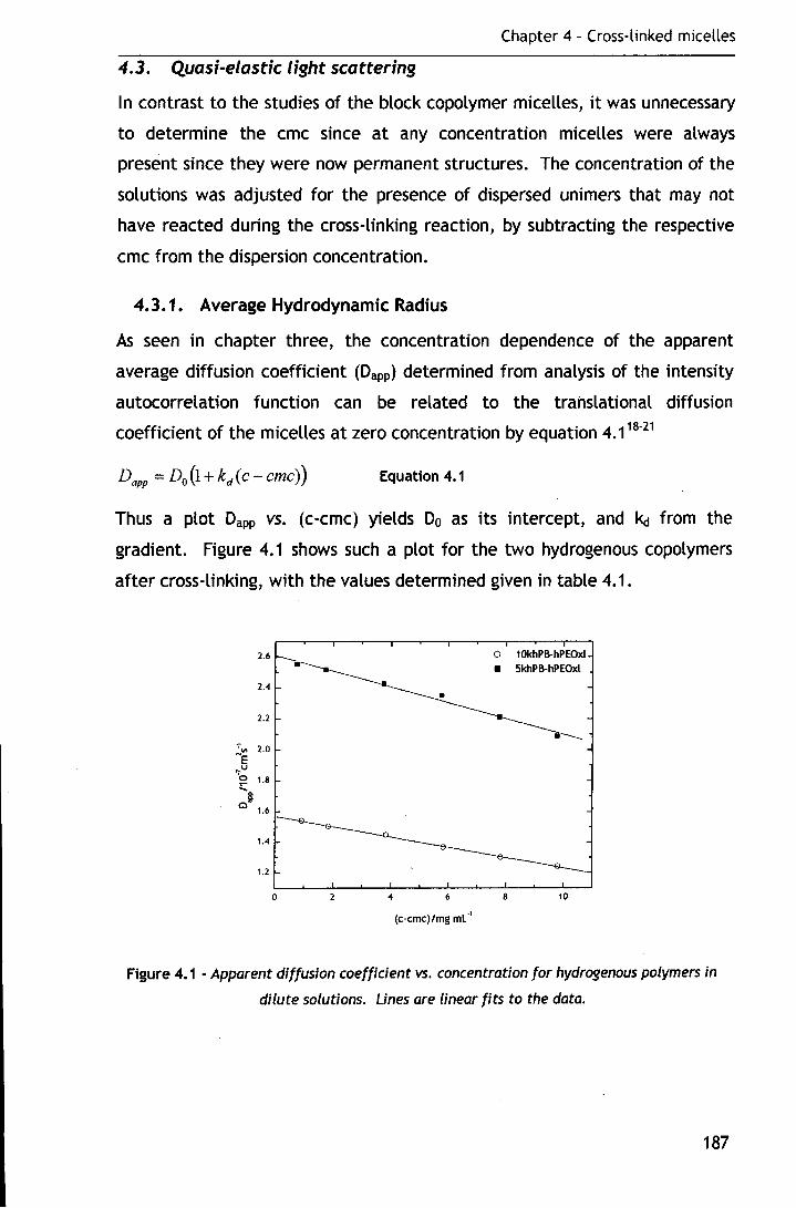
Chapter 4 - Cross-linked micelles
4.3. Quasi-elastk light scattering
In contrast to the studies of the block copolymer micelles, it was unnecessary
to determine the erne since at any concentration micelles were always
present since they were now permanent structures. The concentration of the
solutions was adjusted for the presence of dispersed unimers that may not
have reacted during the cross-linking reaction, by subtracting the respective
erne from the dispersion concentration.
4.3.1. Average Hydrodynamic Radius
As seen in chapter three, the concentration dependence of the apparent
average diffusion coefficient (Dapp) determined from analysis of the intensity
autocorrelation function can be related to the translational diffusion
coefficient of the micelles at zero concentration by equation 4.1 18-21
Equation 4. 1
Thus a plot Dapp vs. (c-cmc) yields Do as its intercept, and ~ from the
gradient. Figure 4.1 shows such a plot for the two hydrogenous copolymers
after cross-linking, with the values determined given in table 4. 1.
2.6 o 10khPB-hPEOxl • 5khPB-hPEOxl
2.4 •
2.2
0 4 6 8 10
(c-cmc)/mg ml·'
Figure 4.1 - Apparent diffusion coefficient vs. concentration for hydrogenous polymers in
dilute solutions. Lines are linear fits to the data.
187

Chapter 4 - Cross-linked micelles
Copolymer
10k hPB-hPEOxl 1.567±0.006 156.1 ±0.5 -0.0216±0.002
5k hPB-hPEOxl 2.610±0.018 93.8±0.6 -0.0195±0.003
Table 4. 1 - Diffusion coefficient, Hydrodynamic radii, and second virial diffusion coefficient
calculated from extrapolation to infinite dilute for hydrogenous polymers.
The radii determined for the cross-linked micelles are smaller than those
determined prior to core cross-linking (viz. 168.2 and 135.8A for the 10k and
5k respectively). This result is not unexpected, since the core has essentially
undergone a . polymerisation reaction, and with this one would normally
associate a decrease in volume. Other reports also note a decrease in radii on
cross-linking. · In common with the reports of Won and eo-workers, 3 the
reduction in the core volume exceeds that associated with the densification of
rubber. From crude estimates based on the van der Waals radii and the
length of carbon-carbon bonds the decrease in core radii upon polymerisation
would be anticipated to be of the order of 7%, a value in the region of that
observed.
One striking feature of the data is the reversal in sign of the diffusion second
virial coefficient for the 5k micelles, from positive to negative, such now that
both molecular weights exhibit values of the same sign. This may be due to
the presence of residual inorganic salts from the cross-linking reaction, whose
concentrations are close to that of the copolymer in the dispersion, giving rise
to bridging effects in the corona of the micelles, and thus making them
attractive rather than repulsive to one another.
The scaling relationship proposed by Halperin22 is now perhaps more relevant
since the cross-linked micelles could be viewed as star polymers having a
number of arms equal to the association number. According to Halperin the
micelle radius can be related to the degree of polymerisation of both blocks
and the segment length by equation 4.2.
Equation 4.2
where N8 is the degree of polymerisation of the core block, NA is the degree of
polymerisation of the shell block, and a is the segment length, the value of
which was given in chapter three (4.01A)23
188

Chapter 4 - Cross-linked micelles
Table 4.2 details t~e values expected from equation 4.2, and the
experimentally determined values for the micelles both before and after
cross-linking.
Copolymer Rh/A RlX ~:R
1 Ok hPB-hPEO (B14Es9) - micelles 135.8 92.4 1.470
5k hPB-hPEO (B21E164) - micelles 168.2 146.6 1.147
10k hPB-hPEO (B14Es9)- xl micelles 93.8 92.4 1.015
5k hPB-hPEO (B21E164) -xl micelles 156.1 146.6 1.065
Table 4.2 - Hydrodynamic radii determined by QELS, and theoretical radii determined using
Halperin's star model (equation 4.2),R, with Rh:R being the ratio of the experimental and
theoretical radii.
lt is evident from table 4.2 that the correlation between the experimentally
determined value and the theoretically expected value is better for the
micelles after they have been cross-linked. This is likely to be due to the
origins of the model being in the description of star polymers, and as the
cross-linked micelles behave more like star polymers due to their fixed core
than the micelles, better agreement would be expected.
4.3.2. Concentration effects
In common with the micelles, the effect of concentration upon the size
distribution of the cross-linked micelles was investigated at concentrations as
high as 100 mg ml·1 for both molecular weights. Figures 4.2 and 4.3 show the
size distributions, obtained from CONTIN24 analysis, for 10k hPB-hPEO and 5k
hPB-hPEO respectively.
189
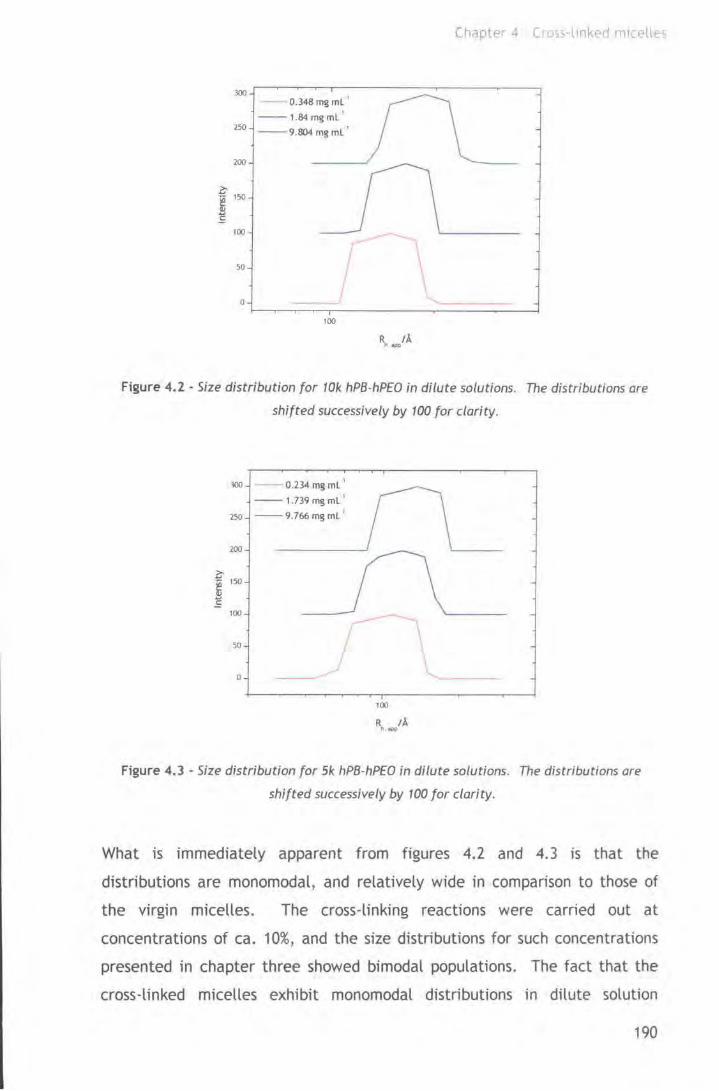
Chapter 4 Cr oss-ltnked mKell:?-s
300 0.348 mgml '
--1.84 mg ml ' 250 --9.804mgml '
200
?;-
~ 150
.E 100
50
0
100
R. _ tA
Figure 4.2- Size distribution for 101< hPB-hPEO in dilute solutions. The distributions are
shifted successively by 100 for clarity.
300 - 0.234 mg ml '
-- 1.739 mg ml '
250 --9.766mgml '
200
.~ 150
~ 100
50
0
100
R lA ··-Figure 4.3 ·Size distribution for 51< hPB-hPEO in dilute solutions. The distributions are
shifted successively by 100 for clarity.
What is immediately apparent from figures 4.2 and 4.3 is that the
distributions are monomodal, and relatively wide in comparison to those of
the virgin micelles. The cross-linking reactions were carried out at
concentrations of ea. 10%, and the size distributions for such concentrations
presented in chapter three showed bimodal populations. The fact that the
cross-linked micelles exhibit monomodal distributions in dilute solution
190
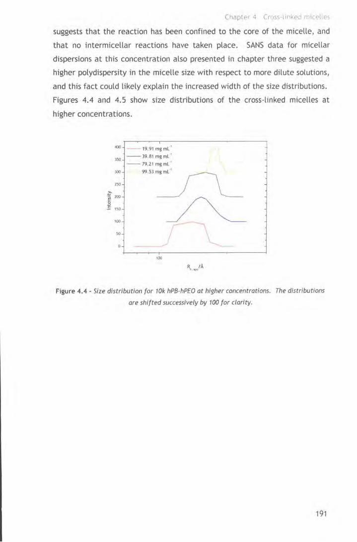
Chapter 4 (r'r;ss·tlnked 111C(·llL·s
suggests that the reaction has been confined to the core of the micelle, and
that no intermicellar reactions have taken place. SANS data for micellar
dispersions at this concentration also presented in chapter three suggested a
higher polydispersity in the micelle size with respect to more dilute solutions,
and this fact could likely explain the increased width of the size distributions.
Figures 4.4 and 4.5 show size distributions of the cross-linked micelles at
higher concentrations.
400 --19.91 mgml 1
350 --39.81 mgml 1
--79.11 mgml 1
lOO 99.53 mg ml 1
250
.?1100 § E 150
100
50
0
100
f\.Ojl<> tA
Figure 4.4 - Size distribution for 10k hPB-hPEO at higher concentrations. The distributions
are shifted successively by 100 for clarity.
191
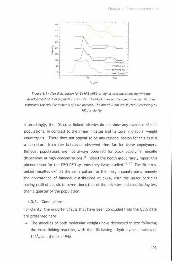
<lOO
3~0
.lOO
250
:;-·- 200
~ £ 150
100
50
0
to 100
'\, tA ....
19.80mg ml '
-- 39.87 mg ml '
--80.04 mg ml '
100.72 mg ml
1000
Figure 4.5- Size distribution for Sk hPB·hPEO at higher concentrations showing the
development of dual populations at c>2%. The black lines on the cumulative distributions
represent the relative amounts of each present. The distributions are shifted successively by
100 for clarity
Interestingly, the 10k cross-linked micelles do not show any evidence of dual
populations, in contrast to the virgin micelles and its lower molecular weight
counterpart. There does not appear to be any rational reason for this as it is
a departure from the behaviour observed thus far for these copolymers.
Bimodal populations are not always observed for block copolymer micelle
dispersions at high concentrations, 25 indeed the Booth group rarely report this
phenomenon for the PBO-PEO systems they have studied. 26•
27 The Sk cross
linked micelles exhibit the same pattern as their virgin counterparts, namely
the appearance of bimodal distributions at c>2%, with the larger particles
having radii of ea. six to seven times that of the micel~es and constituting less
than a quarter of the population.
4.3.3. Conclusions
For clarity, the important facts that have been concluded from the QELS data
are presented here.
• The micelles of both molecular weights have decreased in size following
the cross-linking reaction, with the 10k having a hydrodynamic radius of
156A, and the 5k of 94A.
192
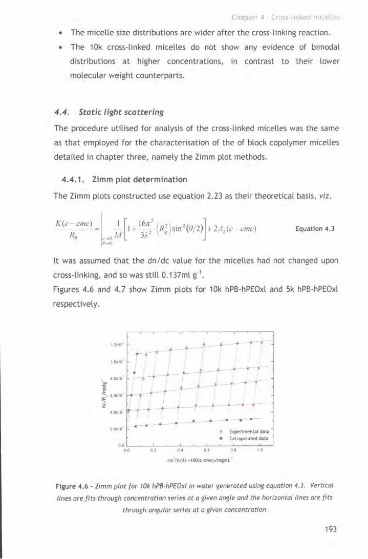
Chapter 4 Cross-lmked '111Celles
• The micelle size distributions are wider after the cross-linking reaction.
• The 10k cross-linked micelles do not show any evidence of bimodal
distributions at higher concentrations, in contrast to their lower
molecular weight counterparts.
4.4 . Static light scattering
The procedure utilised for analysis of the cross-linked micelles was the same
as that employed for the characterisation of the of block copolymer micelles
detailed in chapter three, namely the Zimm plot methods.
4.4. 1. Zimm plot determination
The Zimm plots constructed use equation 2.23 as their theoretical basis, viz.
K(c -cmc) = 1 [ 16JT~ ( "' ) . ' ( I )] M l+)'T R; Sin~ e 2 +2A1(c-cmc)
c->0 / ,
Equation 4. 3
o ... o
lt was assumed that the dn/dc value for the micelles had not changed upon
cross-linking, and so was still 0.137ml g·1•
Figures 4.6 and 4.7 show Zimm plots for 10k hPB-hPEOxl and Sk hPB-hPEOxl
respectively.
1.2X10
1.0x10
• - -~ _.J.- - -t-- -r-r 1 I I 4-- __ !_ ___ ._ -
-r- t- -, I _l
-.-+ +- --4.0x10 -· _ _. _- .. -.- . 2.0x10 EJ<perimental data
• Extrapolated data
sin1(lll2) •100(c-cmc)/mgml1
Figure 4.6 - Zimm plot for 10k hPB-hPEOxl in water generated using equation 4.3. Vertical
lines are fits through concentration series at a given angle and the horizontal lines are fits
through angular series at a given concentration.
193

1.0x10
1 .5~10 .,., ] ...... r:! 1 Ox10 u ...
5.0x10
Chapte1 4 Ct o~<; llnkE?CI n tcelles
Experimental data • Extrapolated data
f •
.. • 1
.1- • • 1
0.1 0.4 0.6 0.8 I 0
sin1(1!12) .. 100(c·cmc)/mgml '
Figure 4. 7 - Zimm plot for 5k hPB-hPEOxl in water generated using equation 4.3. Vertical
lines are fits through concentration series at a given angle and the horizontal lines are fits
through angular series at a given concentration.
The parameters determined from the extrapolations to zero angle and zero
concentration are listed in table 4.3.
Polymer
1 Ok hPB-hPEOxl
5k hPB-hPEOxl
4.275x10⁶ ± 4.5x10⁴
1 .195x 1 07 ± 1 . 85x 1 05
5.083x10'4
8.393x10'4
470
undefined
Table 4.3 - Molecular weights, second viria/ diffusion coefficients (A1) and radii of gyration
calculated from extrapolated data in figures 4.6 and 4.7.
What is immediately apparent from table 4.3 are the differences in the
molecular weight of the two species of cross-linked micelles. Similar to the
virgin micelles, the lower molecular weight copolymer micelles display a
higher molecular weight. Again, perhaps the only rational explanation is that
of experimental error, with the quality of the data being quite poor. In this
respect the observation of a negative radius of gyration for the Sk cross-linked
micelles clearly indicates other factors at work. This may result from the
unusual solvent conditions imparted from the presence of the inorganic slats
in the dispersions. The radius of gyration determined for the 1 Ok cross-linked
194
Chapter 4 - Cross-linked micelles
micelles is not that expected for micelles behaving as hard spheres then Rg:Rh
=O.n should apply.28 The observed value is ea. 3, more in line with the value
expected for cylindrical morphology. SAXS and SANS data presented later in
this chapter suggest micelles are spherical in nature, calling into question the
validity of the SLS data.
Using equation 3.16, and the dn/dc values calculated for the individual
blocks, along with their respective molecular weights the true value of the
micelle molecular weight can be calculated. 29 These values are listed in table
4.4.
Polymer Ma,pp/g mor1 Mw/g mor
10k hPB-hPEOxl· 4.275x10⁶ ± 4.5x10⁴ 3.168x10⁶ ± 3.518x10⁴
5k hPB-hPEOxl 1.195x10⁷ ± 1.85x10⁵ 8.851x10⁶ ± 1.379x10⁵
Table 4.4 - True molecular weights of 10k hPB-hPEOxl and 5k hPB-hPEOxl calculated using
equation 3. 16.
4.4.3. Conclusions
As was the case with the virgin micelles, interpretation of the SLS data is
open to question. The molecular weights and radii obtained from the data do
not make a great deal of sense with respect to the QELS data and theoretical
predictions. One can only assume that the dubious quality of the data is
either a phenomenon of the particular system or due to experimental error.
The presence of the inorganic salts is likely to complicate the behaviour of
the micelles due to the changes in the solvent properties for the coronal
brush.
4.5. Small-angle X-ray scattering
4. 5. 1. Introduction
The SAXS experiments were carried out under the same conditions reported
earlier, with the exception of 020 being the solvent as opposed to HzO, due to
the solutions being obtained by direct dilution from the reaction mixture. As
195
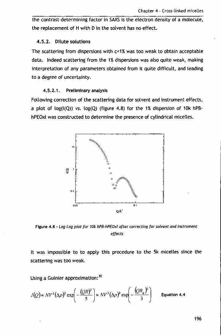
Chapter 4 - Cross-linked micelles
the contrast-determining factor in SAXS is the electron density of a molecule,
the replacement of H with Din the solvent has no effect.
4. 5. 2. Dilute solutions
The scattering from dispersions with c<1% was too weak to obtain acceptable
data. Indeed scattering from the 1% dispersions was also quite weak, making
interpretation of any parameters obtained from it quite difficult, and leading
to a degree of uncertainty.
4.5.2.1. Preliminary analysis
Following correction of the scattering data for solvent and instrument effects,
a plot of log(I(Q)) vs. log(Q) (figure 4.8) for the 1% dispersion of 10k hPB
hPEOxl was constructed to determine the presence of cylindrical micelles.
10
g1 0
0
0.1
0.01 0.1
Q!A"'
Figure 4.8 - Log-Log plot for 10k hPB-hPEOxl after correcting for solvent and instrument
effects
lt was impossible to to apply this procedure to the Sk micelles since the
scattering was too weak.
Using a Guinier approximation: 30
Equation 4.4
196

Chapter 4 - Cross-linked micelles
both the radius of gyration and the radius of a sphere can be determined from
the scattering data. A plot of ln(I(Q))vs. Q2 gives a gradient of -R2 /5 or -
R/ /3. Figure 4. 9 shows a Guinier approximation for the 10k cross-linked
micelles.
OL-~-L~--L-~-L~--L-~-L~~
0.0002 0.0004 0.0006 0.0008 0.0010 0.0012 0.0014
Q'tA:'
Figure 4.9- Guinier approximation for 10k hPB-hPEOxl constructed using equation 4.6.
Sphere radius determined from linear fit is 116 A.
The radius determined from a linear fit to the data is 116A. This is smaller
than the hydrodynamic radius of 156A determined from the QELS
experiments. lt is larger than the value of 70A obtained from SAXS
experiments on the virgin micelles however, in contrast to the observations
made in the QELS experiments where the micelles contracted in size following
cross-linking. As was stated earlier, the scattering from the dilute dispersions
before and after cross-linking was relatively weak and so values obtained from
them should be treated with caution.
4.5.2.2. Fitting to a core-shell model
The spherical core-shell model employed to fit the micelle data was also
utilised here. 31 The model was described in some detail in section 3.4.2.2,
and so will not be discussed. Dr Richard Heenan's FISH2 analysis software was
used to fit the data; with the same strategy used earlier. 32
197

lO
1S
g 10
0
ChaptPr 4 Cros~-llnkt?d ;••c.,·\le;;
Figure 4.10 shows the fit obtained for 1 Ok hPB-hPEOxl using the core-shell
model in both linear and semi-logarithmic form, with the parameters
extracted from the fit given in table 4.5.
a) b)
10
\ g1
0.1
0.00 0.02 0.1>1 0.06
Q/A1
0.03 0. 10 0.12 0.00 0.05 0 10
QJA '
Figure 4.10- F;ts obtained to 1% dispersion data for 10k hPB-hPEOxl using the FJSH2
software program. a) shows a linear intensity scale, and b) shows a logarithmic intensity
scale. Red lines are fits to the data
Parameter 1 Ok hPB-hPEOxl
Re/A 23
Res/A 98
Rs/A 75
~ 0.17
Table 4.5 -Parameters obtained from fits to 10k hPB-hPEOxl, shown in figure 4. 14, using the
core-shell model
lt is evident from figure 4.10, that the model does not really fit the data, and
so the dimensions obtained from it should not be taken as absolute.
The micelle dimensions obtained from the core-shell fit to the data are larger
than those of the virgin micelles, which was also seen from the Guinier
approximation. Again this contradicts the QELS data, but as the scattering
observed in the SAXS experiments was relatively weak, and the fit to the data
not exact, it is perhaps more prudent to trust the QELS data.
198
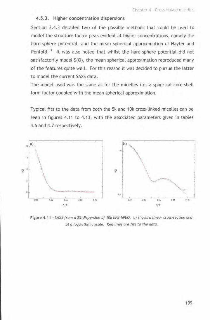
Chapter 4 Cross-linked mJCPlles
4.5.3. Higher concentration dispersions
Section 3.4.3 detailed two of the possible methods that could be used to
model the structure factor peak evident at higher concentrations, namely the
hard-sphere potential, and the mean spherical approximation of Hayter and
Penfold. 33 lt was also noted that whilst the hard-sphere potential did not
satisfactorily model S(Q), the mean spherical approximation reproduced many
of the features quite well. for this reason it was decided to pursue the latter
to model the current SAXS data.
The model used was the same as for the micelles i.e. a spherical core-shell
form factor coupled with the mean spherical approximation.
Typical fits to the data from both the Sk and 1 Ok cross-linked micelles can be
seen in figures 4.11 to 4.13 , with the associated parameters given in tables
4.6 and 4.7 respectively.
20 a) .
15
f! 10
0
10
0.1
0.02 0.04 0.06 0.08 0.10 0.02 0.04 0.06 0.08 0 10
QIA' Q/A'
Figure 4.11 - SAXS from a 2% dispersion of 10k hPB-hP£0. a) shows a linear cross-section and
b) a logarithmic scale. Red lines are fits to the data.
199

Chapter 4 Cross-t1nked miCelles
10 a) b)
0-01
10
a ::: I
0.1 '--'--~---~--'---'---'---'---'----' 0.04 0.06 0.08 0. 10 0.12 0 .1• 0.02 004 006 0 .08 0.10 012
Qt!.'' QIA·'
Figure 4.12 - SAXS from a 4% dispersion of 5k hPB-hP£0. a) shows a linear cross-section and
b) a logarithmic scale. Red lines are fits to the data.
0.02 0.03 004 0.05 0.06 0.07 0.08 00'1 0.10 0.11
Qt/>:'
....
0.02 0 0) 0.04 0.05 0.06 0 07 0.08 0 0'1 0 10 0 "
QIA'
Figure 4.13 - SAXS from a 10% dispersion of 10k hPB-hPEO. a) shows a linear cross-section
and b) a logarithmic scale. Red lines are fits to the data.
200
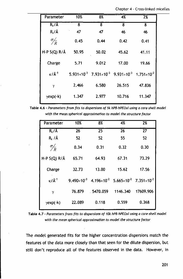
Chapter 4 - Cross-linked micelles
Parameter 10% 8% 4% 2%
Re/A 8 8 8 8
RsiA 47 47 46 46
1R 0.45 0.44 0.42 0.41
H-P S(Q) R/A 50.95 50.02 45.62 41.11
Charge 5.71 9.012 17.00 19.66
x/A-1 5.931x10"3 7.931x10"3 9.931x10"3 1.751x10"2
y 2.466 6.580 26.515 47.836
yexp(-k) 1.347 2.9n 10.716 11.347
Table 4.6 - Parameters from fits to dispersions of 5k hPB-hPEOxl using a core-shell model
with the mean spherical approximation to model the structure factor
Parameter 10% 8% 4% 2%
Re/A 26 25 26 27
Rs lA 52 52 55 52
1R 0.34 0.31 0.32 0.30
H-P S(Q) RIA 65.71 64.93 67.31 73.29
Charge 32.73 13.00 15.62 17.56
x/A-1 9.490x10"3 4.196x10"2 5.665x10"2 7.351 x10"2
y 76.879 5470.059 1146.340 17609.906
yexp(-k) 22.089 0.118 0.559 0.368
Table 4. 7 - Parameters from fits to dispersions of 10k hPB-hPEOxl using a core-shell model
with the mean spherical approximation to model the structure factor
The model generated fits for the higher concentration dispersions match the
features of the data more closely than that seen for the dilute dispersion, but
still don't reproduce all of the features observed in the data. However, in
201

common with the Vlrgm micelles, the low SAXS contrast hinders any
quantitative treatment of the data.
4. 5.4. Comparison between virgin and cross-linked micelles
Comparisons between the SAXS data for the micelles before and after cross
linking is not one that can be done quantitatively due to the nature of the fits
generated using the core shell model, as the fits do not reproduce all the
features in the data. lt is however, a useful exercise to show changes in the
behaviour of the micelles before and after cross-linking.
Figures 4.14-4.17 show the SAXS data from the virgin and cross-linked micelles
plotted on the same axes. Representative samples of the concentration and
molecular weight effects have been given. Table 4.8 details the dimensions
determined from the fits before and after cross-linking.
10
g 1
0.1
\ • • •
"vu"gm" m1cettes • cross-linked micelles
.. •
·~ ":.·
0 Ol O.Ool 0.06 0 Ill 0 10 0.12 n 14
Figure 4.14 • SAXS data from 10k 2% hPB-hPEO before and after cross-linking. Unes are fits
to the data.
202
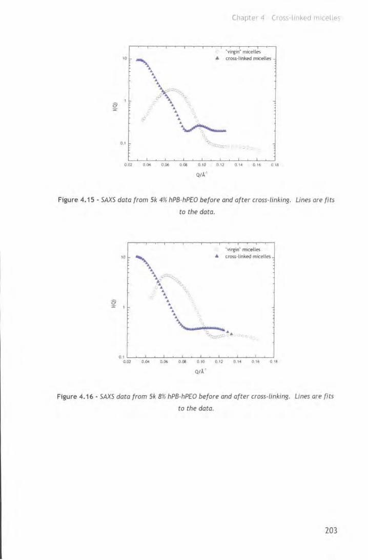
Chaptet 4 Ct oss l1oked 1111C,.?lles
!0
0.1
.__.\ ... ... ... ...
x~ ~~ ... ... " ... ... .,. .
"v11-gm" micelles io cross-linked micelles
·~
O.o2 0.04 0.06 0.08 0.10 0 12 0. 1~ 0.16 0.18
QIA '
Figure 4.15 - SAXS data from 51< 4% hPB-hPEO before and after cross-linking. Lines are fits
to the data.
10 "\ ... ·· --~ . ·, ~ ... ... • • ... ... • ... ... ...
'-·
"vu-gm" mtce lles io cross·linked micelles
e. ...... ~~-- ...
0.1 L_..._....L..__.___Jc._...___.___....__._.__....__.._-~.__._..._-L-_,
0.02 0.04 0.06 0.08 0 10 0.12 0.1~ 0 16 018
QIA ,
Figure 4.16- SAXS data from 5k 8% hPB-hPEO before and after cross-linking. Lines are fits
to the data.
203

Chapter 4 Cross·LH1ked mtcelle!1
' virgm" micelles • cross-linked micelles
10
0. 1 ........... ---'---'--"---'---'---'---'--'.__.__.___.___.__.__....._.1-..J 0.00 0 02 0.04 0.06 0.08 0, tO 0.12 0.14 0.16
QIA '
Figure 4.17- SAXS data from 10k 10% hPB-hP£0 before and after cross-linking. Lines are fits
to the data.
10k hPB-hPEO Sk hPB-hPEO
Cone/% Parameter Virgin xl Virgin xl
micelles micelles micelles micelles
10 Re/A 15 26 6 8
Rs lA 43 52 32 47
yexp( -k) 23.083 22.089 13.901 1.347
8 Rei A 16 25 6 8
Rs lA 43 52 30 47
yexp( -k) 23.465 0.118 20.477 2.977
4 Re/A 13 26 6 8
Rs I A 48 55 30 46
yexp( -k) 29.057 0.559 21.294 10.716
2 Re/A 11 27 6 8
Rs /A 59 52 25 46
yexp( -k) 62.594 0.368 27.194 11.347
Table 4.8 -Micelle dimensions determined from fits to SAXS data before and after cross-
linking reaction.
204
Chapter 4 - Cross-linked micelles
What is immediately apparent from figures 4.14-4.17 is the change in the
shape of the structure factor peak. In all of the samples characterised, with
the exception of the 10k 10% dispersion, the peak has largely disappeared,
with it no longer showing a clearly pronounced maximum as it does in the
virgin micelles. This appears to be caused by the shift in the entire data to
lower Q values, which one could associate with an increase in dimensions of
the micelles, a fact supported by the parameters from fits to the data shown
in table 4.8. However, the change in shape could also be due to decreased
interactions between the micelles, reducing the degree of ordering in the
system, and thus the intermicellar interference that gives rise to the structure
factor peak. As stated in chapter three, yexp( -k) is the contact potential
between a macroion pair, which for uncharged species such as those
encountered here, can serve as an indication as to the strength of interaction
between the micelles. For any given concentration at either of the two
molecular weights the value of yexp( -k) is smaller for the micelles after cross
linking than before, supporting the notion of decreased interaction between
them. However, as the model does not reproduce the features of the
scattering data to an acceptable degree, values obtained from fitting the data
should be treated with caution. The safest conclusion is that the contact
potential suggests reduced interaction on cross-linking.
The interpretation of the scattering data from the cross-linked micelles is
made troublesome by the residual inorganic salts from the cross-linking
reaction. These effect the properties of the solvent, in terms of its
thermodynamic quality, and serve to increase the SAXS contrast by virtue of
their large numbers of electrons. Thus quantitative comparisons between the
two sets of scattering data are impossible.
4.5.5. Conclusions
In common with the virgin micelles, the low SAXS contrast hindered attempts
to produce a quantitative picture of the micelles in terms of their dimensions
and interactions. Scattering from the dilute regime was even less pronounced
than for the virgin micelles, consequently obtaining quantitative of sufficient
quality was difficult if not impossible. For clarity the main conclusions that
can be inferred from the data are presented below.
205
Chapter 4 - Cross-linked micelles
• Fits to the dilute dispersion data for 10k hPB-hPEOxl, using a spherical
core shell model, suggest the micelles have a core radius of 23A
surrounded by a shell that is 75A thick, giving a total micelle radius of
98A, larger than from the micelles prior to cross-linking. These values
should be treated with caution since the fit does not match the data
exactly.
• The scattering from Sk hPB-hPEOxl at 1% was too weak to fit.
• The mean spherical approximation due to Hayter and Penfold was used to
model the scattering from the higher concentration data, but with limited
success.
• Fits to the higher concentration data suggest 1 Ok hPB-hPEOxl micelles
have a core radius of 26A and a shell thickness of 52A, whilst their Sk
counterparts have a core of 8A and a shell of 46A, both of which are
larger than for the virgin micelles.
• The structure factor peak due to intermicellar interactions is not as
pronounced for the cross-linked micelle dispersions. There is support
from interpretations of fits to the data that this is due to a decrease in
intermicellar interactions.
• A detailed comparison of the data with that of the virgin micelles was
impossible due to the different solvent conditions under which the
scattering experiments were carried out.
4.6. Small-angle Neutron scattering
4. 6. 1. Introduction
The protocol for the SANS experiments on the cross-linked micelles was the
same as that employed for the virgin micelles, the same range of
concentrations and contrasts were explored, except for the fully hydrogenous
micelles where the maximum concentration probed was 10%.
206

~ 0.1
Q ij 0.01
~
I El
·6
Chapter 4 Cro:)s·llnkt?d m~c.elle!.
4.6.2. Dilute dispersions
4.6.2.1. Preliminary treatment
Double logarithmic plots showed no Q-1 dependencies indicative of cylindrical
micelles. 34 Typical plots for 1% dispersions of both molecular weights for all
contrasts are shown in figure 4.18. The reader is referred to pg 139 for the
equivalent plots for the virgin micelles.
0.01 0.1
Ql~:'
...
hPB·hPE hPB·dPE dPB·hPEO
10 )_
-5 0.1
a ~ ....... 0.01
~
lE l
hf>B.I>PEO hPB·dPEO dPB·hPEO
1£~ ,__~......._ _____ ....__.._~-~-~
0.01 01
QtA'
Figure 4.18- Double logarithmic plots for a)Sk and b) 10k dispersion of cross-linked
micelles. Representative error bars are shown for clarity.
The Guinier approximation was applied to the dilute solution data. Typical
plots are shown in figure 4.19 again for both copolymers and all three
contrasts, with the respective results obtained detailed in table 4. 9.
-- ________ ___ hPB·hPEO hPB·dPEO dPB·hPEO
..... __ -
..,... E ~
~ 18 c ....
1,5
1.0
M
0.0
-0.5
·1.0
·1.5
·20
-- - .....L...
PB-hPEO hPB·dPEO dPB·hPEO
0.0000 0.0002 0.~ 0 .0006 0.0006 0.0010 0.0011
Q'tA'
00000 0.0002 0 ~ 0 0006 0 0006 0.0010 0 0011
Q'tA'
Figure 4.19 - Guinier plots for 1% dispersions of a) Sk and b) 10k cross-linked micelles
generated using equation 4. 6. Lines are linear fits to the data
207
Chapter 4 - Cro~s-linked micelles
Isotopic Sphere Radius/ A
variation Cone/% 0.2 0.4 0.6 1
hPB-hPEO Sk micelles 76 74 77 74
xl micelles n/a 64 67 69
10k micelles 132 131 130 130
xl micelles 82 88 84 85
hPB-dPEO Sk micelles 126 125 120 123
xl micelles n/a 99 66 85
10k micelles 161 173 168 169
xl micelles 100 88 88 87
dPB-hPEO Sk micelles n/a n/a 48 61
xl micelles n/a n/a n/a n/a
10k micelles 56 65 60 66
xl micelles n/a n/a 44 52
Table 4. 9 - Sphere radii determined using Guinier approximation for micelles both before
and after cross-linking for both molecular weight series and all contrasts. Isotopic variant in
bold is the part of the molecule scattering the radiation. nl a indicates scattering was too
weak to give acceptable values.
lt is evident from table 4. 9 that in all cases the size of the micelles has
decreased following cross-linking. This is consistent with the observations of
the QELS experiments, and in line with the result expected.
4.6.2.2. Fitting to a core-shell model
The model used to fit the data from the cross-linked micelles was that
employed for the virgin micelles described in chapter three, i.e. a spherical
core-shell form factor, with uniform core density and a parabolic volume
fraction profile in the shell.
The FISH2 analysis software was used to fit the data, fixing the volume
fraction of water in the innermost sub-shell of the corona.
Figures 4.20 to 4.22 show representative fits for the different contrasts and
concentrations explored for the two molecular weights, with the parameters
from all of the fits for the dilute dispersions given in tables 4.10 and 4.11.
208
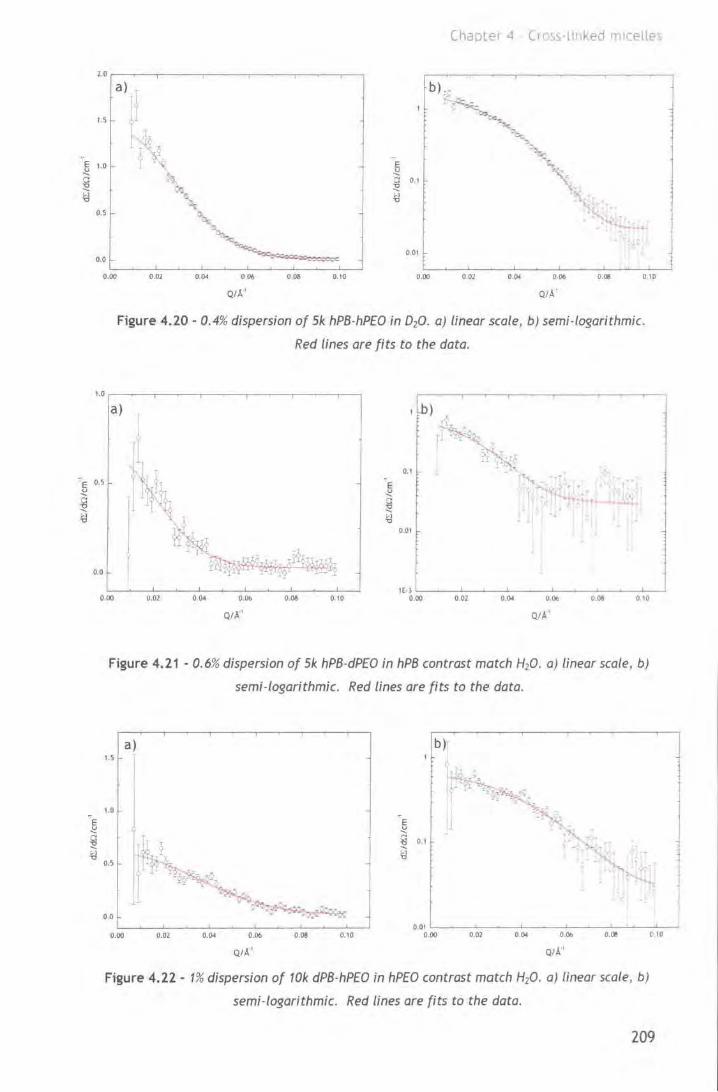
~E
~
~ le!
2.0 ,..---~-.----.----.--~-.----.-----,
a) .
1.5
1.0
0.5
0.0
0.00 0.02
·.
0.11• 0116
QIA'
0.08 0.10
Chapte1 4 Cross-lmked m1cell~s
~ ~ O. l
"' ,
001
b) .
0.00 0.02 0.04 006
QIA'
0.08 0 . 1~
Figure 4. 20 - 0.4% dispersion of 5k hPB-hPEO in 0 20. a) linear scale, b) semi-logarithmic.
Red lines are fits to the data.
1.0.----.----.----.----.----,---. a)
0.00
' I
0.02 004 0.06
QIA·'
) ,
0.1
0.01
0.08 0.10 0.02 0.04 006
QIA '
0.03 0.10
Figure 4.21 - 0.6% dispersion of 5k hPB·dPEO in hPB contrast match H20 . a) linear scale, b)
semi-logarithmic. Red lines are fits to the data.
a) b) 1.5
~~ -~~
~- . :r;,.k -" . .. 1.0
~ ~
E ~ c '0 .... 0.1
>l , 0.5
00
0.00 0.02 0.04 0.06
QtA'
003 0.10
"' '0
0.01 0.00 0.02 004 0.06 o.oe
QtA''
Figure 4.22 • 1% dispersion of 101< dPB·hPEO in hPEO contrast match H20. a) linear scale, b)
semi-logarithmic. Red lines are fits to the data.
C.tO
209
! l 1 <

Chapter 4 - Cross-linked micelles
Copolymer Cone/% ReA RsA t\pc/101ocm-2 t\pJ1010cm-2 1R ~
hPB-hPEO 0.2· Scattering too weak to fit
0.4 14 53 -4.Bn -1.033 0.20 0.82
0.6 14 53 -4.762 -1.148 0.20 0.8
1.0 14 52 -4.590 -1.320 0.20 o.n hPB-dPEO 0.2 Scattering too weak to fit
0.4 19 53 -1.078 1.078 0.67 0.82
0.6 19 55 -1.198 1.198 0.54 0.80
1.0 21 54 -1.198 1.198 0.64 0.80
dPB-hPEO 0.2
0.4 Scattering too weak to fit
0.6
1.0 19 6.180 0 0.27
Table 4.10- Parameters obtained from 5k cross-linked micellar dispersions fitted to the
core-shell model shown using FISH 2.
Copolymer Cone/% ReA RsA t\pcf101ucm-" t\pJ101ucm-" 1R ~
hPB-hPEO 0.2 29 79 -5.049 -0.861 0.25 0.85
0.4 29 76 -4.8n -1.033 0.15 0.82
0.6 24 74 -4.475 -1.435 0.15 0.80
1.0 25 74 -4.647 -1.263 0.15 0.78
hPB-dPEO 0.2 29 61 -0.899 0.899 0.41 0.85
0.4 29 61 -1.078 1.078 0.37 0.82
0.6 30 59 -1.198 1.198 0.28 0.80
1.0 30 58 -1.318 1.318 0.20 0.78
dPB-hPEO 0.2
0.4 Scattering too weak to fit
0.6 37 6.180 0.20
1.0 37 6.180 0.20.
Table 4.11 -Parameters obtained from 10k cross-linked micellar dispersions fitted to the
core-shell model shown using FISH 2.
210
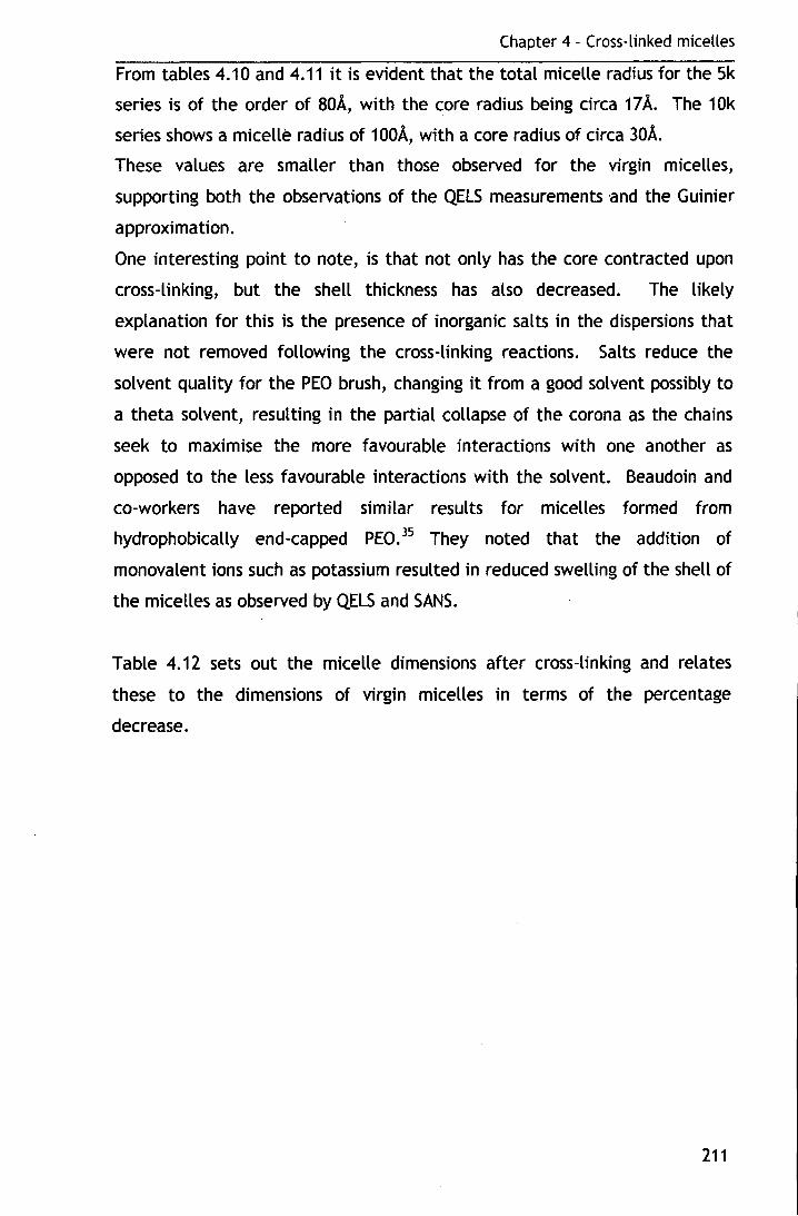
Chapter 4 - Cross-linked micelles
From tables 4.10 and 4.11 it is evident that the total micelle radius for the 5k
series is of the order of 80A, with the ~ore radius being circa 17 A. The 1 Ok
series shows a micelle radius of 1 OOA, with a core radius of circa 30A.
These values are smaller than those observed for the virgin micelles,
supporting both the observations of the QELS measurements and the Guinier
approximation.
One interesting point to note, is that not only has the core contracted upon
cross-linking, but the shell thickness has also decreased. The likely
explanation for this is the presence of inorganic salts in the dispersions that
were not removed following the cross-linking reactions. Salts reduce the
solvent quality for the PEO brush, changing it from a good solvent possibly to
a theta solvent, resulting in the partial collapse of the corona as the chains
seek to maximise the more favourable interactions with one another as
opposed to the less favourable interactions with the solvent. Beaudoin and
eo-workers have reported similar results for micelles formed from
hydrophobically end-capped PEO. 35 They noted that the addition of
monovalent ions such as potassium resulted in reduced swelling of the shell of
the micelles as observed by QELS and SANS.
Table 4.12 sets out the micelle dimensions after cross-linking and relates
these to the dimensions of virgin micelles in terms of the percentage
decrease.
211

Chapter 4 - Cross-linked micelles
Copolymer Cone/% Sk series 10k series
Re/A %- RJA %- Re/A %- RJA %-
hPB-hPEO 0.2 Scattering too weak 29 17 79 31
0.4 14 26 53 15 29 28 76 30
0.6 14 . 26 53 10 24 38 74 34
1.0 14 30 52 10 25 34 74 35
hPB-dPEO 0.2 Scattering too weak 29 28 61 48
0.4 19 21 53 45 29 34 61 45
0.6 21 16 55 41 30 29 59 48
1.0 19 24 54 41 30 33 58 46
dPB-hPEO 0.2 Scattering too weak
0.4 Scattering too weak
to fit to fit
0.6 37 21 - -1."0 19 30 - - 37 18 - -
Table 4.12- Change in radii relative to the virgin micelles. %-calculated by 1-(xl
micelle/virgin)
Table 4.12 demonstrates that there is a finite change in the micelle
dimensions, ranging from 16-38% for the core radius, and 10-48% for the shell
thickness. These are a larger relative change than the 13% decrease in core
radius reported by Won et al. for cylindrical micelles of PB-PEO. 3
In chapter three, the association numbers for the micelles were calculated on
the basis of the core radius and the volume of the poly(butadiene) block. This
is not possible for the cross-linked micelles since the core no longer consists
of chains that are independent of one another, but of chains that are
covalently bonded to each other. Under these circumstances perhaps a
realistic assumption to make is that the association number of the micelles
remains unchanged from the value obtained prior to cross-linking, i.e. the
value determined at 10%. This can be justified on the basis that once the
micelle has been cross-linked, just one covalent bond per chain is sufficient to
prevent the chain leaving the micelle. On this assumption, it is possible to
calculate the distance of separation between the PEO chains on the surface of
the core, and relate this to the unperturbed radius of gyration of the PEO
212
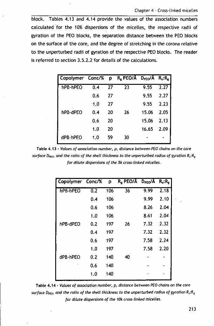
Chapter 4 - Cross-linked micelles
block. Tables 4.13 and 4.14 provide the values of the association numbers
calculated ·for the 10% dispersions of the micelles, the respective radii of
gyration of the PEO blocks, the separation distance between the PEO blocks
on the surface of the core, and the degree of stretching in the corona relative
to the unperturbed radii of gyration of the respective PEO blocks. The reader
is referred to section 3.5.2.2 for details of the calculations.
Copolymer Cone/% p Rg PEO/A OpEofA Rs:Rg
hPB-hPEO 0.4 27 23 9.55 2.27
0.6 27 9.55 2.27
1.0 27 9.55 2.23
hPB-dPEO 0.4 20 26 15.06 2.05
0.6 20 15.06 2.13
1.0 20 16.65 2.09
dPB-hPEO 1.0 59 30 - -
Table 4. 13 - Values of association number, p, distance between PEO chains on the core
surface DPEo, and the ratio of the shell thickness to the unperturbed radius of gyration Rs:R8
for dilute dispersions of the Sk cross-linked micelles.
Copolymer Cone/% p R8 PEO/A OpEofA Rs:R8
hPB-hPEO 0.2 106 36 9.99 2.18
0.4 106 9.99 2.10
0.6 106 8.26 2.04
1.0 106 8.61 2.04
hPB-dPEO 0.2 197 26 7.32 2.32
0.4 197 7.32 2.32
0.6 197 7.58 2.24
1.0 197 7.58 2.20
dPB-hPEO 0.2 140 40
0.6 140
1.0 140
Table 4.14 - Values of association number, p, distance between PEO chains on the core
surface DPEo, and the ratio of the shell thickness to the unperturbed radius of gyration Rs:R9
for dilute dispersions of the 10k cross-linked micelles.
213

Chapter 4 - Cross-linked micelles
The two molecular weight series cross-linked micelles show some similarities
in their behaviour following cross-linking. With the exception of the Sk hPB
dPEO cross-linked micelles, they all show a reduction in the separation
distance between PEO chains on the core surface. One explanation for the
unusual behaviour of the Sk hPB-dPEO species is the association number used
in the calculations. All of the values of p were based upon the core
dimensions determined from fits to the data at the concentration the
reactions were carried out, i.e. 10%. The Sk hPB-dPEO micelles gave a
slightly smaller core radius, and therefore association number, than the more
dilute dispersions. This gives rise to a larger separation distance than that
observed for the dilute dispersions, a result that is quite unexpected.
Because the association numbers determined for the Sk micelles were modest
in size (<50), any small .change in the core radius affects the association
number greatly. Consequently the real association number may be larger
than quoted, and thus the PEO chain separation distance may have decreased
along with the others.
4.6.2.3. Comparison with theory
Scaling relationships due to Daoud and Cotton, 36 Halperin, 22 and Zuhlina and
Birshtein37 were used in chapter three to compare the micelle dimensions
obtained through fits to the data with those expected from theory. The
scaling relationships were given in table 3.25 in chapter three. Those due to
Halperin were used to calculate the expected micelle dimensions that are
given in table 4.15.
214
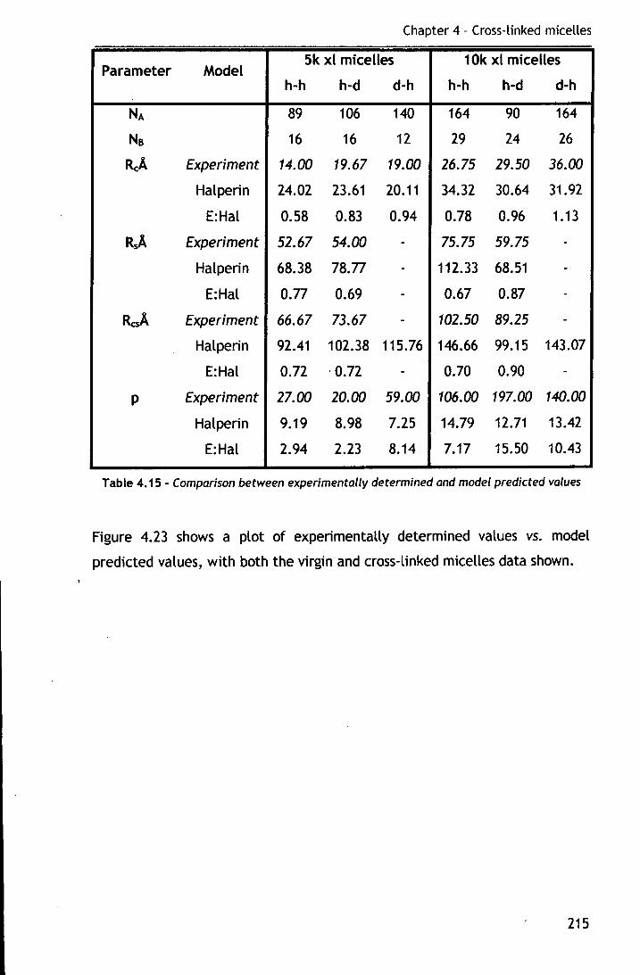
Chapter 4 - Cross-linked micelles
Parameter Model 5k xl micelles 1 Ok xl micelles
h-h h-d d-h h-h h-d d-h
NA 89 106 140 164 90 164
Na 16 16 12 29 24 26
ReA Experiment 14.00 19.67 19.00 26.75 29.50 36.00
Halperin 24.02 23.61 20.11 34.32 30.64 31.92
E:Hal 0.58 0.83 0.94 0.78 0.96 1.13
Rsl Experiment 52.67 54.00 - 75.75 59.75 -
Halperin 68.38 78.n - 112.33 68.51 -E:Hal o.n 0.69 - 0.67 0.87 -
RcsA Experiment 66.67 73.67 - 102.50 89.25 -
Halperin 92.41 102.38 115.76 146.66 99.15 143.07
E:Hal 0.72 . 0.72 - 0.70 0.90 -
p Experiment 27.00 20.00 59.00 106.00 197.00 140.00
Halperin 9.19 8.98 7.25 14.79 12.71 13.42
E:Hal 2.94 2.23 8.14 7.17 15.50 10.43
Table 4. 15 - Comparison between experimentally determined and model predicted values
Figure 4.23 shows a plot of experimentally determined values vs. model
predicted values, with both the virgin and cross-linked micelles data shown.
215
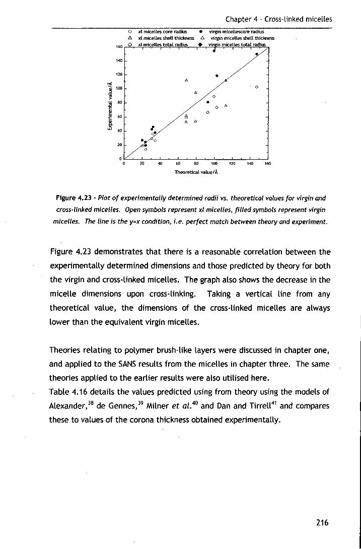
o<{
o xl micelles core radius A xl micelles shell thickness
160 <> xl micelles total radius
140
120 1:>
Chapter 4 - Cross-linked micelles
• virgin micellescore radius A virgin micelles shell thickness
+ vi 'n micelles total radius
•
• ~ 100
0 Cl.
0
2i 80 • 0 Cl.
1:
~ 0 'I: 60 A
! 1:> 1:>
40 I ~
• 0 20 • 0
0 0 20 40 60 80 100 120 140 160
Theoretical value/A
Figure 4.23 - Plot of experimentally determined radii vs. theoretical values for virgin and
cross-linked micelles. Open symbols represent xl micelles, filled symbols represent virgin
micelles. The line is the y=x condition, i.e. perfect match between theory and experiment.
Figure 4.23 demonstrates that there is a reasonable correlation between the
experimentally determined dimensions and those predicted by theory for both
the virgin and cross-linked micelles. The graph also shows the decrease in the
micelle dimensions upon cross-linking. Taking a vertical line from any
theoretical value, the dimensions of the cross-linked micelles are always
lower than the equivalent virgin micelles.
Theories relating to polymer brush-like layers were discussed in chapter one,
and applied to the SANS results from the micelles in chapter three. The same
theories applied to the earlier results were also utilised here.
Table 4.16 details the values predicted t,~sing from theory using the models of
Alexander, 38 de Gennes, 39 Milner et al. 40 and Dan and Tirrell41 and compares
these to values of the corona thickness obtained experimentally.
216

Chapter 4 - Cross-linked micelles
Parameter Model 5k series 10k series
hPB-hPEO xl hPB-dPEO xl hPB-hPEO xl hPB-dPEO x
NA 89 106 164 90
D/A 9.55 15.59 9.21 7.45
cr o.1n 0.066 0.190 0.290
Experiment/ A 52.67 54.00 75.75 59.75
htA Alexander 200.33 172.75 378.17 238.59
E:Alex 0.263 0.313 0.200 0.250
hi A de Gennes 41.83 36.07 78.96 49.81
E:dG 1.259 1.497 0.959 1.199
h/A Milner 44.64 38.50 84.27 53.17
E:Milner 1.180 1.403 0.899 1.124
h/A D&T 69.11 72.19 131.54 103.48
E:D&T 0.762 0.748 0.576 o.5n
Table 4. 16 - Comparison between experimental data and theoretically predicted values for
the corona thickness based on polymer brush theory
Figure 4.24 shows a plot of the ratio between experimental and theoretical
data vs. the degree of polymerisation for the corona block for the micelles
before and after the cross-linking reaction.
217
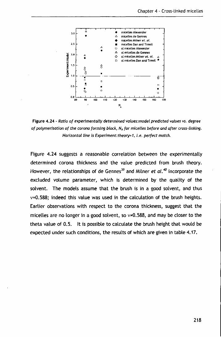
Chapter 4 - Cross-linked micelles
A • micelles Alexender 3.0 • 6. micelles de Gennes
• micelles Milner et. al . 2.5 • micelles Dan and Tirrett
A 0 xl micelles Alexender • 6. xl micelles de Gennes 12.0 A 0 xl micelles Mitner et. al. • A
,.; 0 xt micelles Dan and Tirrett • c: ~ 1.5 A
A 0 'C 0 8. A
..1S 1.0 0 • • ti 0
0
0.5 ~ 0 • • • CO 0
0
0.0 80 90 100 110 120 130 140 150 160 170
N A
Figure 4.24- Ratio of experimentally determined values: model predicted values vs. degree
of polymerisation of the corona forming block, NA for micelles before and after cross-linking.
Horizontal line is Experiment:theory=1, i.e. perfect match.
Figure 4.24 suggests a reasonable correlation between the experimentally
determined corona thickness and the value predicted from brush theory.
However, the relationships of de Gennes39 and Milner et a/.40 incorporate the
excluded volume parameter, which is determined by the quality of the
solvent. The models assume that the brush is in a good solvent, and thus
v=0.588; indeed this value was used in the calculation of the brush heights.
Earlier observations with respect to the corona thickness, suggest that the
micelles are no longer in a good solvent, so v~0.588, and may be closer to the
theta value of 0.5. lt is possible to calculate the brush height that would be
expected under such conditions, the results of which are given in table 4.17.
118
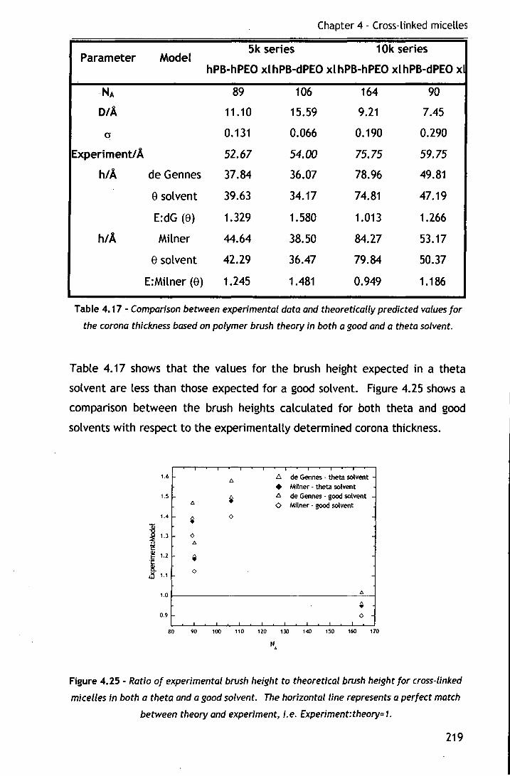
Chapter 4 - Cross-linked micelles
Parameter Model 5k series 10k series
hPB-hPEO xlhPB-dPEO xlhPB-hPEO xlhPB-dPEO x
NA 89 106 164 90
D/A 11.10 15.59 9.21 7.45
0' 0.131 0.066 0.190 0.290
ExperimenU A 52.67 54.00 75.75 59.75
h/A de Gennes 37.84 36.07 78.96 49.81
8 solvent 39.63 34.17 74.81 47.19
E:dG (8) 1.329 1.580 1.013 1.266
hi A Milner 44.64 38.50 84.27 53.17
8 solvent 42.29 36.47 79.84 50.37
E:Milner (8) 1.245 1.481 0.949 1.186
Table 4.17 - Comparison between experimental data and theoretically predicted values for
the corona thickness based on polymer brush theory in both a good and a theta solvent.
Table 4.17 shows that the values for the brush height expected in a theta
solvent are less than those expected for a good solvent. Figure 4.25 shows a
comparison between the brush heights calculated for both theta and good
solvents with respect to the experimentally determined corona thickness.
1.6 L de Germes - theta solvent A • Milner - theta solvent
1.5 ~ tl de Gennes - good solvent
A <> Milner- good solvent
1.4 ~ <>
a:; ~ 1.3 <>
~ A
~ 1.2 ~ ·r::
!1.1 <>
1.0 A
~ 0.9 <>
80 90 100 110 120 130 140 150 160 170
N A
Figure 4.25- Ratio of experimental brush height to theoretical brush height for cross-linked
micelles in both a theta and a good solvent. The horizontal line represents a perfect match
between theory and experiment, i.e. Experiment:theory=1.
219
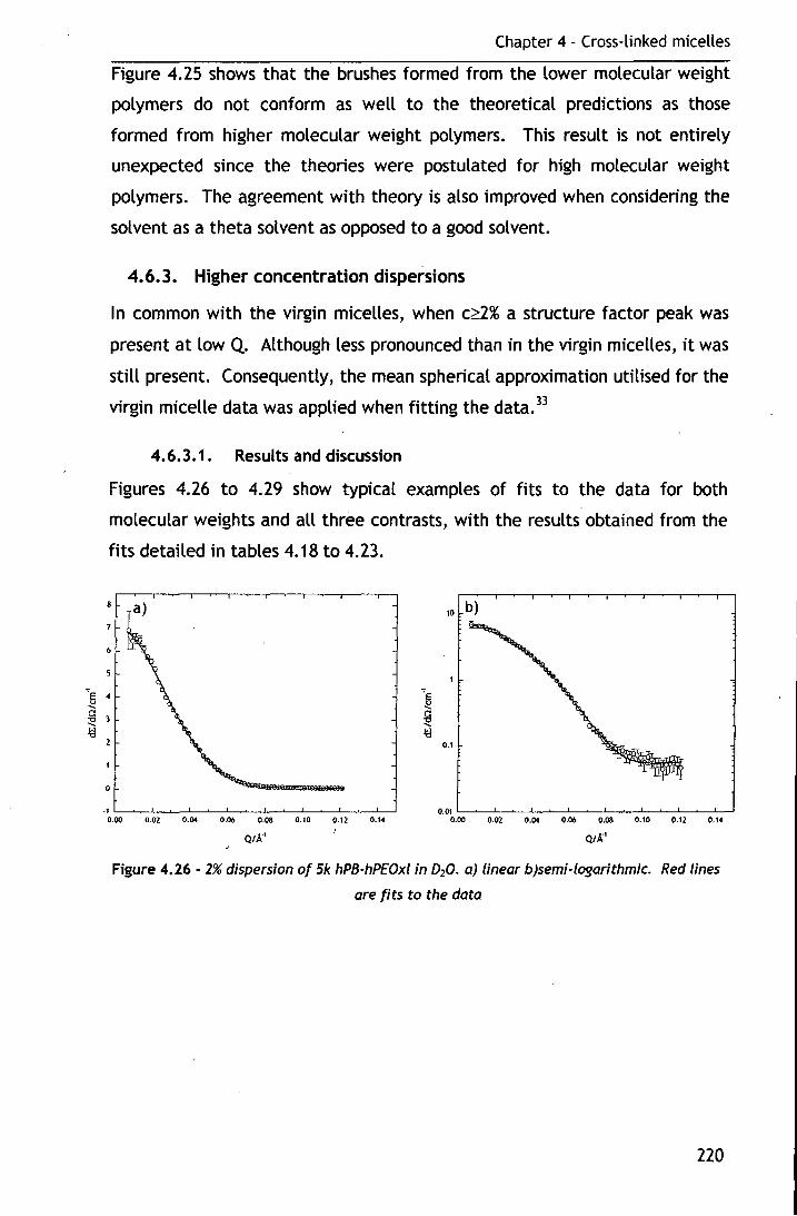
Chapter 4- Cross-linked micelles
Figure 4.25 shows that the brushes formed from the lower molecular weight
polymers do not conform as well to the theoretical predictions as those
formed from higher molecular weight polymers. This result is not entirely
unexpected since the theories were postulated for high molecular weight
polymers. The agreement with theory is also improved when considering the
solvent as a theta solvent as opposed to a good solvent.
4.6.3. Higher concentration dispersions
In common with the virgin micelles, when c;?:2% a structure factor peak was
present at low Q. Although less pronounced than in the virgin micelles, it was
still present. Consequently, the mean spherical approximation utilised for the
virgin micelle data was applied when fitting the data. 33
4.6.3.1. Results and discussion
Figures 4.26 to 4.29 show typical examples of fits to the data for both
molecular weights and all three contrasts, with the results obtained from the
fits detailed in tables 4.18 to 4.23.
10 b)
0.1
0.01 L-......--L~-'--~-'--....___,~___,_~_,__~.1.--J 0.00 0.02 0.04 0.06 0.08 0.10 0.12 0.14
QJA"'
Figure 4.26- 2% dispersion of Sk hPB-hPEOxl in D20. a) linear b)semi-logarithmic. Red lines
are fits to the data
220
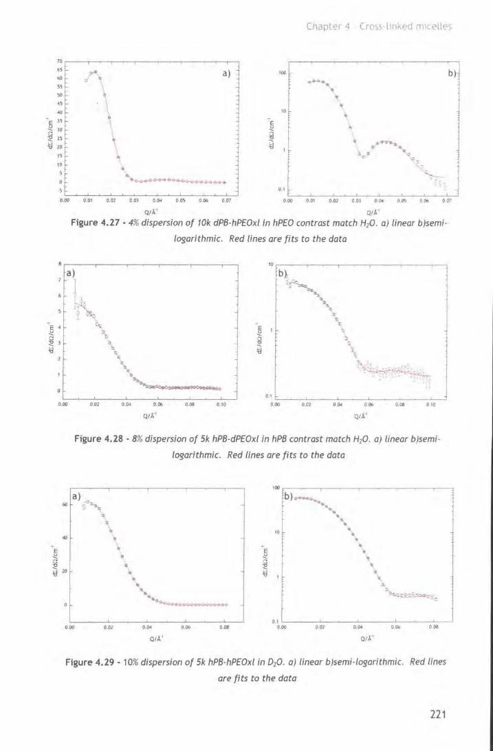
E V .... ~ ,., "
Chapte:-1 4 Cross·ltnkec! m1celtt:'s
70
65 o'" a) 100 b) bO .. .. .......... 55
" 50 ~ .. ~5
40 10 • - .. 35 \ E 30 ~ • 25 ~ • ....
=- "*·~·- . 20 .. , " )::: :
.. c 15 • .:;
10
"' .;; 4 ~
0 ~~··~·~~~~~~ 0. 1
0.00 0 01 0.02 0.03 o.a. 0.05 O.Ob 0.07 0.00 0,()1 0.02 O.ol o.a. 0()'; O.Ob Or!l
QIA:' QIA·'
Figure 4.27- 4% dispersion of 10k dPB·hPEOxl in hPEO contrast match H20. a) linear b)semi·
logarithmic. Red lines are fits to the data
10~~--,------.------------~----.--.
:;
\,~-
0 -~-!111 ....... .....,
0.1 '------'-~---'------'---~--'----..1-.....J 0.00 0 .02 0.04 0.06
Q/A.,
008 0.10 0.00 002 o.a. 006
QIA '
0.08 010
40
0.00
Figure 4.28- 8% dispersion of Sk hPB·dPEOxl in hPB contrast match H20 . a) linear b)semi·
logarithmic. Red lines are fits to the data
• •
o.oz
•
.. 4o
o.a. 0.06 0.08
QIA'
100 .-------.-----,------.------;-----,
10 ~ .. • • •
' ;)
0.
~~:~=::
0.1 1......--~--'-------'--------'---~---'----' 0.00 0.02 o.a. 006 008
QIA '
Figure 4.29- 10% dispersion of Sk hPB-hPEOxl in 020. a) linear b)semi·logarithmic. Red lines
are fits to the data
221

Chapter 4 - Cross-linked micelles
Parameter 10% 8% 4% 2%
Re/A 14 14 13 12
Rs/A 41 42 44 44
1R 0.747 0.745 0.722 0.723
<l>w 0.50 0.55 0.60 0.65
OpEQ/ A 11.10 11.10 10.30 9.51
Rs:Rg 1.76 1.80 1.89 1.89
H-P S(Q) RIA 48.09 45.36 50.98 50.98
Charge 6.65 6.87 2.25 1.50
x/A"1 3.732x10"3 9.877x10"3 1'. 129x10"2 2.752x10"2
y 3.375 4.347 0.453 0.452
yexp(-k) 2.358 1.774 0.143 0.027
Table 4.18 - Parameters from fits to Sk hPB-hP£0 in D20 2%5ts10%
In common with the virgin micelle data, (cf pg 158) the distinct steps in the
value of <1>w result from the fitting procedure employed; namely fixing the
scattering length densities at values corresponding to a given value of <1>w and
investigating different values of <1>w until an acceptable fit was found.
222
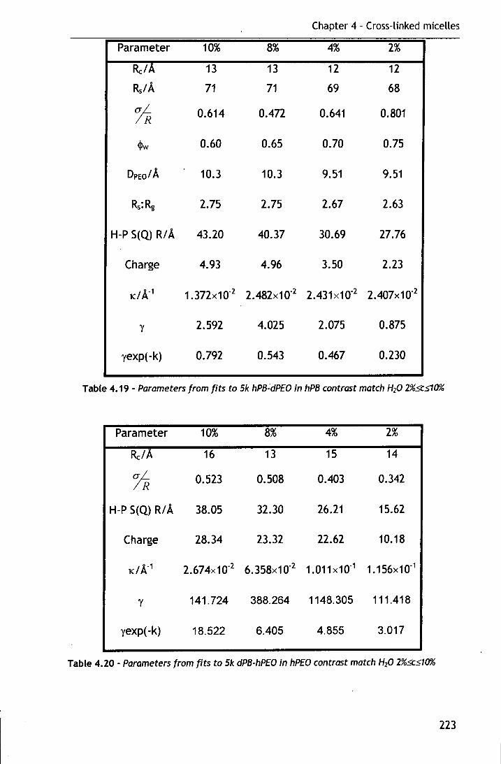
Chapter 4- Cross-linked micelles
Parameter 10% 8% 4% 2%
Re/A 13 13 12 12
RsiA 71 71 69 68
~ 0.614 0.472 0.641 0.801
~w 0.60 0.65 0.70 0.75
OpEQI A 10.3 10.3 9.51 9.51
Rs:Rg 2.75 2.75 2.67 2.63
H-P S(Q) RIA 43.20 40.37 30.69 27.76
Charge 4.93 4.96 3.50 2.23
KIA" 1 1.372x10"2 2.482x10"2 2.431x10"2 2.407x10"2
y 2.592 4.025 2.075 0.875
yexp(-k) 0.792 0.543 0.467 0.230
Table 4.19- Parameters from fits to 5k hPB~dPEO in hPB contrast match H20 2%scst0%
Parameter 10% 8% 4% 2%
Re/A 16 13 15 14
~ 0.523 0.508 0.403 0.342
H-P S(Q) R/A 38.05 32.30 26.21 15.62
Charge 28.34 23.32 22.62 10.18
KIA" 1 2.674x10"2 6.358x10"2 1.011x10"1 1.156x10"1
y 141.724 388.264 1148.305 111.418
yexp(-k) 18.522 6.405 4.855 3.017
Table 4.20- Parameters from fits to 5k dPB-hPEO in hPEO contrast match H20 2%scst0%
223
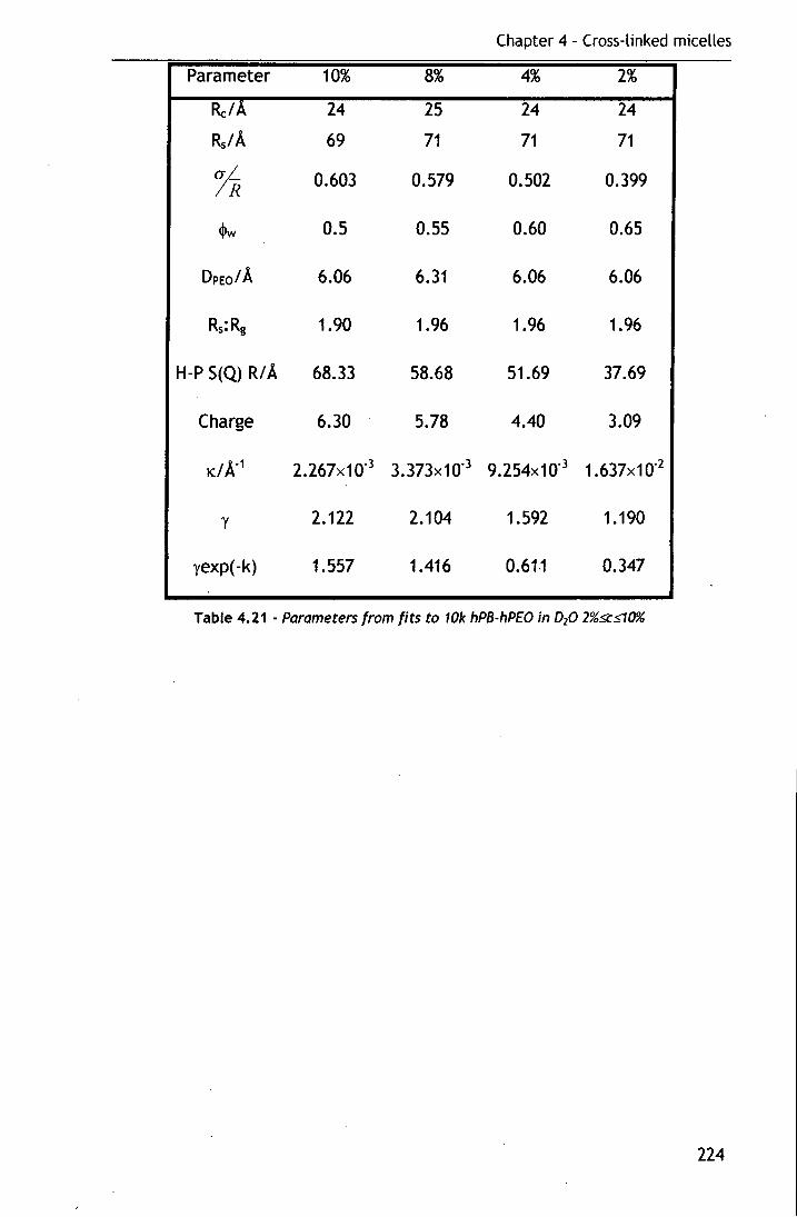
Chapter 4 - Cross-linked micelles
Parameter 10% 8% 4% 2%
Re/A 24 25 24 24
Rs/A 69 71 71 71
~ 0.603 0.579 0.502 0.399
~w 0.5 0.55 0.60 0.65
DPEo/ A 6.06 6.31 6.06 6.06
Rs:Rg 1.90 1.96 1.96 1.96
H-P S(Q) R/A 68.33 58.68 51.69 37.69
Charge 6.30 5.78 4.40 3.09
KIA" 1 2.267x10"3 3.373x10"3 9.254x10"3 1.637x10"2
y 2.122 2.104 1.592 1.190
yexp(-k) 1.557 1.416 0.61.1 0.347
Table 4.21 -Parameters from fits to 10k hPB-hPEO in D20 2%stS10%
224
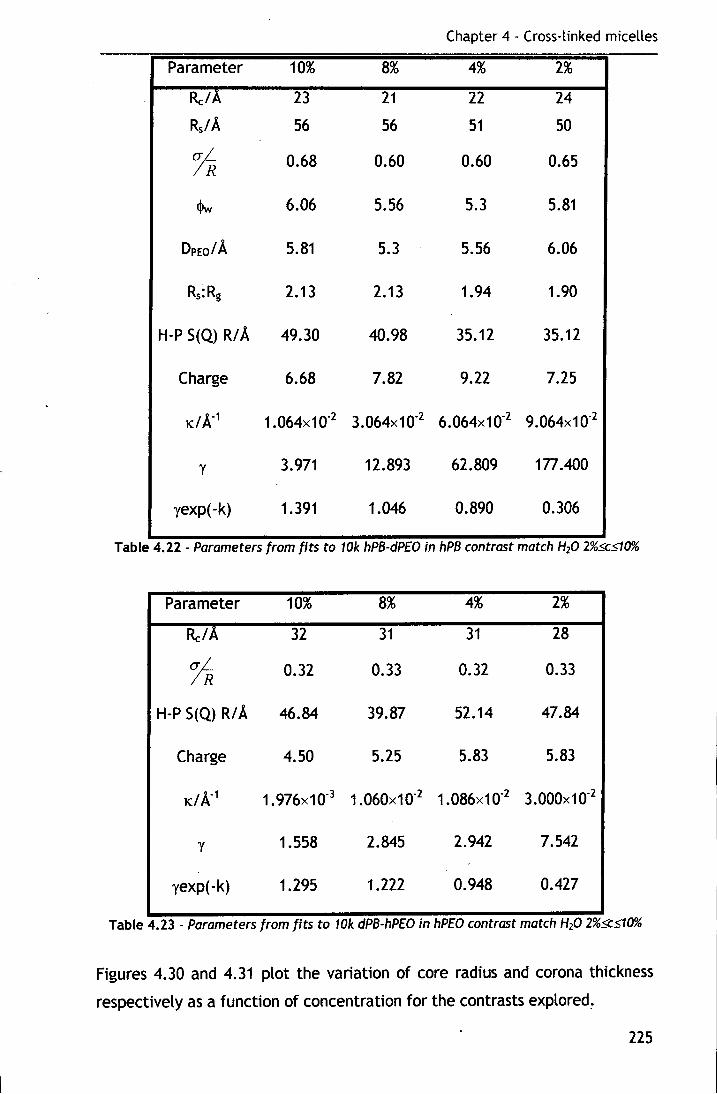
Chapter 4- Cross-linked micelles
Parameter 10% 8% 4% 2%
Re/A 23 21 22 24
RsiA 56 56 51 50
1-R 0.68 0.60 0.60 0.65
$w 6.06 5.56 5.3 5.81
DPEo/ A 5.81 5.3 5.56 6.06
Rs:Rg 2.13 2.13 1.94 1.90
H-P S(Q) R/A 49.30 40.98 35.12 35.12
Charge 6.68 7.82 9.22 7.25
KIA" 1 1.064x10"2 3.064x10"2 6.064x10"2 9.064x10"2
y 3.971 12.893 62.809 1n.40o
yexp(-k) 1.391 1.046 0.890 0.306
Table 4.22- Parameters from fits to 10k hPB-dPEO in hPB contrast match H20 2%SCS10%
Parameter 10% 8% 4% 2%
Re/A 32 31 31 28
1-R 0.32 0.33 0.32 0.33
H-P S(Q) R/A 46.84 39.87 52.14 47.84
Charge 4.50 5.25 5.83 5.83
KIA" 1 1.976x10"3 1.060x10"2 1.086x10"2 3.000x10"2
y 1.558 2.845 2.942 7.542
yexp(-k) 1.295 1.222 0.948 0.427
Table 4.23- Parameters from fits to 10k dPB-hPEO in hPEO contrast match H20 2%scS10%
Figures 4.30 and 4.31 plot the variation of core radius and corona thickness
respectively as a function of concentration for the contrasts explored ..
225

Chapter 4 - Cross-linked micelles
0 5kh-h A 5k h-d 0 5kd-h
• 10kh-h A 10k h-d •• 10k d-h
32 • • • 30
28 • 26
• -<1: 24 0 • • .... ~ 22 "' "' !.!! "' !!! 20
8 18
16 0 <>
14 0 0 0 0 0 "' 12 0 "' 4 6 8 10
Concnetration/%
Figure 4.30- Variation of cross-linked micelle core radius with concentration for the
different molecular weights and contrasts investigated.
0 5kh-h A Skh-d
• 10k h-h E:::. 10kh-d
70 • • • "' "' •
"' 65
~ 60
! u :E 55 ... "' 1:
g 50 u "'
45 0 0
0
40 <(
2 4 6 8 10
Concnetration/%
Figure 4.31 -Variation of cross-linked micelle corona thickness with concentration for the
different molecular weights and contrasts investigated
From the data presented in tables 4.18-4.23, and figures 4.30 and 4.31 the
following trends in the dimensions of cross-linked micelles can be observed.
i.) The core radius increases with concentration for all contrasts of the Sk
series.
226
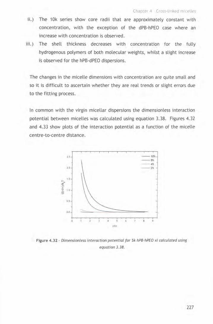
Chupler 4 Cross· l111kC'd m~eell~s
ii.) The 1 Ok series show core radii that are approximately constant with
concentration, with the exception of the dPB-hPEO case where an
increase with concentration is observed.
iii.) The shell thickness decreases with concentration for the fully
hydrogenous polymers of both molecular weights, whilst a slight increase
is observed for the hPB-dPEO dispersions.
The changes in the micelle dimensions with concentration are quite small and
so it is difficult to ascertain whether they are real trends or slight errors due
to the fitting process.
In common with the virgin micellar dispersions the dimensionless interaction
potential between micelles was calculated using equation 3.38. Figures 4.32
and 4.33 show plots of the interaction potential as a function of the micelle
centre-to-centre distance.
2-5 --·~ - -a% -- 4%
2.0 --2%
1.5
~ ;::. .!2 ... 1 0 75
05
0.0
0 4 9
tier
Figure 4.32 - Dimensionless interaction potential for 5k hPB·hP£0 xt calculated using
equation 3.38.
227
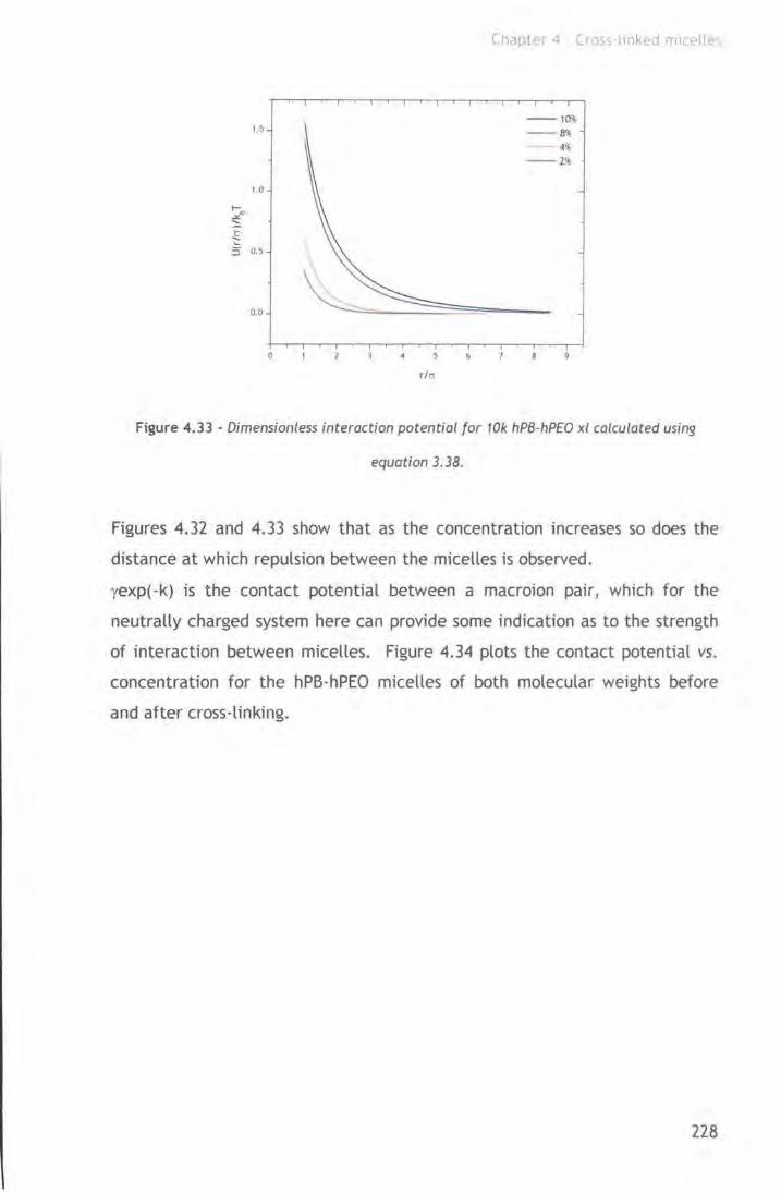
1,5
10
0.0
0
r/r;
Cross·lmkttd mh.ell ~
--10%
--~ 4\
--2\
a 9
Figure 4.33 - Dimensionless interaction potential for 10k hPB-hP£0 xi calculated using
equation 3.38.
Figures 4.32 and 4.33 show that as the concentration increases so does the
distance at which repulsion between the micelles is observed.
yexp(-k) is the contact potential between a macroion pair, which for the
neutrally charged system here can provide some indication as to the strength
of interaction between micelles. Figure 4.34 plots the contact potential vs.
concentration for the hPB-hPEO micelles of both molecular weights before
and after cross-linking.
228
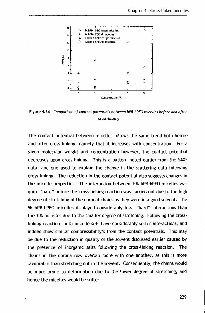
Chapter 4 - Cross-linked micelles
16 0 5k hPB-hPEO virgin micelles
14 • 5k hPB-hPEO xl micelles 6. 10k hPB-hPEO virgin micelles
12 6. 10k hPB-hPEO xl micelles 6
10
~ 8
i 6
:- 6 0
4 .6 0
2 0 • 0 ~ 6
~ 6
0 • 4 6 8 10
Concentration/%
Figure 4.34 - Comparison of contact potentials between hPB-hPEO micelles before and after
cross-linking
The contact potential between micelles follows the same trend both before
and after cross-linking, namely that it increases with concentration. For a
given molecular weight and concentration however, the contact potential
decreases upon cross-linking. This is a pattern noted earlier from the SAXS
data, and one used to explain the change in the scattering data following
cross-linking. The reduction in the contact potential also suggests changes in
the micelle properties. The interaction between 1 Ok hPB-hPEO micelles was
quite "hard" before the cross-linking reaction was carried out due to the high
·degree of stretching of the coronal chains as they were in a good solvent. The
5k hPB-hPEO micelles displayed considerably less "hard" interactions than
the 1 Ok micelles due to the smaller degree of stretching. Following the cross
linking reaction, both micelle sets have considerably softer interactions, and
indeed show similar compressibility's from the contact potentials. This may
be due to the reduction in quality of the solvent discussed earlier caused by
the presence of inorganic salts following the cross-linking reaction. The
chains in the corona now overlap more with one another, as this is more
favourable than stretching out in the solvent. Consequently, the chains would
be more prone to deformation due to the lower degree of stretching, and
hence the micelles would be softer.
229

Chapter -1 Cross-linkt'd mlrPites
Similarly to the v1rgm micelles it is possible to construct reduced force
distance profiles from the interaction potentials,42 shown in figures 4.35 and
4.36 for the 5k hPB-hPEO and the 10k hPB-hPEO respectively. The plots have
been calculated using the excluded volume exponent for a theta solvent.
1E·l
\
0.01
Reduced distance
--1
8'.\,
--4% --2%
Figure 4.35- Reduced force as a function of reduced separation of micelle cores for Sk hPB
hPEO.
0. 1
0.01
1E·~
1E-5
1E·l
Reduced distance
--10%
8'.\,
--4% --2%
().01
Figure 4.36 - Reduced force as a function of reduced separation of micelle cores for 10k
hPB-hPEO.
The profiles in figures 4.35 and 4.36 are similar in nature to those determined
for the virgin micelles, with the magnitude of the reduced force being smaller
230
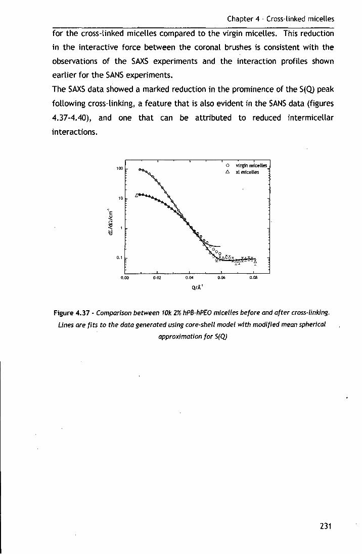
Chapter 4 - Cross-linked micelles
for the cross-linked micelles compared to the virgin micelles. This reduction
in the interactive force between the coronal brushes is consistent with the
observations of the SAXS experiments and the interaction profiles shown
earlier for the SANS experiments.
The SAXS data showed a marked reduction in the prominence of the S(Q) peak
following cross-linking, a feature that is also evident in the SANS data (figures
4.37-4.40), and one that can be attributed to reduced intermicellar
interactions.
100
10
0.1
0.00 0.02 0.04
Qtl>:'
0.06
o virgin micelles D. xl micelles
0.08
Figure 4.37- Comparison between 10k 2% hPB-hPEO micelles before and after cross-linking.
Lines are fits to the data generated using core-shell model with modified mean spherical
approximation for S(Q)
231
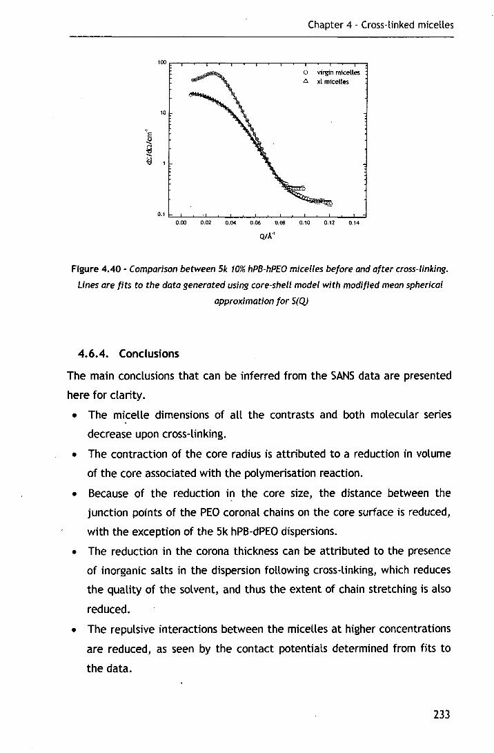
10
Chapter 4 - Cross-linked micelles
o virgin micelles L:. xl micelles
0.00 0.02 0.04 0.06 0.08 0.10 0.12 0.14
QtJ.:'
Figure 4.40 - Comparison between 5k 10% hPB-hPEO micelles before and after cross-linking.
Lines are fits to the data generated using core-shell model with modified mean spherical
approximation for S(Q)
4.6.4. Conclusions
The main conclusions that can be inferred from the SANS data are presented
here for clarity.
• The micelle dimensions of all the contrasts and both molecular series
decrease upon cross-linking.
• The contraction of the core radius is attributed to a reduction in volume
of the core associated with the polymerisation reaction.
• Because of the reduction i~ the core size, the distance between the
junction points of the PEO coronal chains on the core surface is reduced,
with the exception of the Sk hPB-dPEO dispersions.
• The reduction in the corona thickness can be attributed to the presence
of inorganic salts in the dispersion following cross-linking, which reduces
the quality of the solvent, and thus the extent of chain stretching is also
reduced.
• The repulsive interactions between the micelles at higher concentrations
are reduced, as seen by the contact potentials determined from fits to
the data.
233
Chapter 4 - Cross-linked micelles
• The reduction in repulsion between the micelles arises due to a change in
the nature of the coronal brush. Residual salts from the cross-linking
reaction change the brush from a highly stretched incompressible layer,
to one that is quite soft and less stretched.
4. 7. · Final discussion
lt was possible to cross-link the double bonds of the PB core of PB-PEO
micelles in aqueous solution using a redox couple, to generate free radicals at
room temperature. The success of the reaction was determined by the
disappearance of vinyl protons in the 1H NMR spectra. In common with a
similar procedure employed by Won, Davis and Bates, 3 the reaction was
confined to the core of the micelles as confirmed by the monomodal size
distributions seen in QELS experiments. QELS revealed the micelle size was
reduced by 7-30% upon cross-linking, which could be attributed to the
contraction of the micelle core upon polymerisation. Several authors
including Won et al., 3 Wilson and Reiss, 43 and Guo et al. 17 have observed the
same phenomenon.
The concentration dependence of the apparent diffusion coefficient was
found to be negative for both molecular weights, in contrast to the virgin
micelles where the 5k micelles exhibited a positive dependence.
Hydrodynamic radii determined from this concentration dependence were
156A and 94A for the 1 Ok and 5k respectively. The negative dependence of
the apparent diffusion coefficient may be a result of the presence of inorganic
ions remaining in solution from the cross-linking reaction. Such ions could
cause bridging effects between the micelles and result in interaction of an
attractive rather than a repulsive nature. In addition, the presence of such
ions reduces the thermodynamic quality of the solvent for the PEO corona,
resulting in interactions between the micelles being more favourable than
those with the solvent.
The radii of cross-linked micelles determined by QELS showed closer
agreement with Halperin's22 star model than for their virgin counterparts.
This is a little surprising, since although the model has its basis in the
description of star polymers (which is what the cross-linked micelles could be
considered as) it was formulated for a selectively good solvent for the corona
forming block. As already mentioned, the cross-linked micelle size
234
Chapter 4 - Cross-linked micelles
distributions were monomodal in dilute solution. They were however wider
than those of the virgin micelles. This can be attributed to a higher degree of
micelle polydispersity observed from both the QELS and SANS experiments on
the virgin micelles at the concentration the cross-linking reactions were
carried out (10%).
As observed for the virgin micelles, the quality of the SLS data was not good
enough to enable determination of the micelle size or molecular weight. The
cause of the poor quality data was discussed in chapter three, but may
additionally be in some part due to the inorganic salts modifying the
properties of both the micelles and the solvent.
Interpretation of the SAXS data with respect to the virgin micelles was
complicated by the enhanced SAXS contrast in the cross-linked dispersions,
due to the presence of electron-rich inorganic ions. Fits to the dilute
dispersion data were only possible for the higher molecular weight species,
and these did not fully reproduce the data. The results suggested increased
micelle dimensions after cross-linking, contradicting the observations of the
QELS experiments. A possible explanation for this increase in dimensions is
the increased contrast between the scattering centres in the sample, caused
by the residual inorganic ions from the cross-linking reaction. These contain
large numbers of electrons and are likely to be associated with solvent water
molecules both inside the corona of the micelles and in the surrounding
medium. This would result in a greater electron density of both the corona
and the solvent, making it easier to "see" the scattering from the polymer
chains. Consequently, the conditions differ greatly from those of the virgin
micelles, and thus quantitative comparisons of the micelles dimensions are
impossible. A second possible explanation for the increase in micelle
dimensions could be that the residual inorganic salts cause the unimers
present in solution to associate with the micelles, resulting in their increased
size.
Fits to the SANS data show a reduction in the core radius of the micelles of
between 16 and 38%, with the corona thickness ~eing 10-48% smaller in the
cross-linked micelles compared to the virgin case. These two observations 235
Chapter 4 - Cross-linked micelles
support those from the QELS experiments of decreased micelle size upon
cross-linking, with the magnitude ~f the reduction being comparable. The
reduction in core radius was expected, due to the anticipated reduction in
, core volume associated with the polymerisation. Won et al. 3 observed a
similar reduction in the core radius of their PB-PEO micelles, although the
magnitude observed was ea 11 %. lt is noteworthy that the authors did not
determine the corona thickness in the cross-linked micelles. They too used
the same redox couple applied here, and so one might anticipate they would
observe the same effect on the corona thickness seen here.
The reduction in the shell thickness of the micelles upon cross-linking is a
little surprising. One would expect that upon contraction of the core, the
distance between the grafting points of the PEO chains on the surface of the
core would be reduced (this was indeed the case). With such a reduction, one
would be expect an increase in the shell thickness as the chains stretch
further into the solvent in order to minimise the unfavourable contact with
each other and ·maximise favourable contacts with the thermodynamically
good sol vent~ However, considering the conditions under which the
investigations were carried out an explanation for this unusual behaviour
becomes apparent. The dispersions used in the QELS, SAXS and SANS studies
were prepared directly from the cross-linking reaction mixture by dilution
with the appropriate solvent. Consequently, the inorganic salts added to
generate the free-radicals required for the cross-linking reaction remained in
the dispersions. The presence of such ions reduces the thermodynamic
quality of the solvent for PEO, resulting in it no longer being a good solvent.
Therefore it is no longer favourable for the chains to stretch away from the
core surface to interact with the solvent; instead, interactions with
neighbouring chains become more favourable, and thus a partial collapse of
the coronal brush is observed. Support for this hypothesis is found in the work
of Beaudoin and eo-workers. 35
Upon cross-linking the core of the micelles perhaps a reasonable assumption
to make is the association number remains unchanged. Such an assumption
can be justified by the fact that only one cross-link per copolymer chain
would be sufficient to prevent the c:;hain leaving the micelle. Using this
assumption the distance between the PEO chains on the core surface was
calculated. In all instances except the 5k hPB-dPEO micelles a reduction in
236
Chapter 4 - Cross-linked micelles
the distance between grafting points was observed. The likely explanation for
this anomalous result lies in the value used for the association number. The
1 0% dispersion of the 5k HPB-dPEO micelles had a small association number of
20, with some of the more dilute dispersions exhibiting higher values. As the
association numbers for the 5k micelles were low to moderate, any slight
change in the core radius resulted in a dramatic change in the association
number.
Calculation of the expected micelle radii based upon Halperin's star model
produced better agreement that could have been anticipated as the model
was formulated for a highly selective good solvent, which was no longer the
case for these dispersions.
Comparison of the corona thickness to the theoretically predicted brush
height using the models applied to the virgin micelles revealed better
agreement for the cross-linked as opposed to the virgin micelles. The
relationships of de Gennes39 and Milner et al. 40 produced the best agreement,
when good solvent conditions were applied but even better when theta
solvent relations were used. The agreement was also better for the longest
forming corona chain. Perhaps the reason for the improved agreement of
these models over that of Dan and Tirrell41 is that the former two
relationships allow incorporation of the solvent quality, whereas the latter
relationship assumes instead the brush is in a good solvent, which as eluded to
earlier is not the case here.
Fitting of the SAXS data from the higher concentration dispersions and
subsequent comparison to the virgin micelle case was complicated by the
presence of the contrast enhancing inorganic ions. The mean spherical
approximation33 produced fits that matched the features of the data more
closely than for the virgin micelles, but the different solvent conditions
between the two sets of dispersions made quantitative comparisons
impossible. The structure factor peak wa·s much less pronounced in the cross
linked micelles compared to the virgin micelles suggesting reduced
intermicellar interactions.
Comparison of the contact potential between the micelles both before and
after cross-linking revealed that for any given molecular weight/concentration
237

Chapter 4 - Cross-linked micelles
combination the contact potential was lower for the cross-linked micelles.
Such a comparison, although not quantitative could be taken as indicative of a
reduction in the micelle interactions following cross-linking.
Fits to the data suggested increased micelle dimensions for both molecular
weights after cross-linking, contradicting both the QELS and the SANS data
discussed earlier. As with the SAXS from dilute dispersions such an increase
can be attributed to the enhanced contrast resulting in more of the micelle
being "seen".
In common with the SAXS data the SANS data from the higher concentration
dispersions shows a greatly reduced structure factor peak when compared to
the virgin micelles. The mean spherical approximation provided excellent
reproduction of the features of the data in the same manner that was
observed for the virgin micelles. Again comparison of the contact potentials
reveals that those of the cross-linked micelles are smaller for a given
molecular weight/concentration combination, suggesting reduced micelle
interactions.
The nature of the interaction potentials appears to have changed upon cross
linking. The lower concentration dispersions (where the structure factor peak ' is still evident) show softer tails at low separations when compared to their
virgin counterparts, which were approaching hard sphere-like interactions. As
the concentration increases the tails become softer, and extend to marginally
longer separations than observed for the virgin micelles (ea. eight times the
diameter as opposed to seven). This suggests the micelle interactions have
become softer, likely due to the reduced degree of stretching discussed
earlier. The reduced force-distance profiles are similar to those of the virgin
micelles and indeed those reported in the literature,42'
44'
45 with the
magnitude of the force smaller than that of the former.
238

Chapter 4- Cross-linked micelles
4.8. Glossary of symbols
The symbols used in the body of the text and the equations are defined here
in the order in which they appear in the text.
4.8.1. Quasi-Elastic Light Scattering
Dapp
erne
Do
k<t
apparent diffusion coefficient
critical micelle concentration
diffusion coefficient at infinite dilute
diffusion second virial coefficient
concentration
apparent hydrodynamic radius
micelle radius
degree of polymerisation of core forming B block
degree of polymerisation of corona forming A block
segment length
4.8.3. Static Light Scattering
K optical constant
c dispersion concentration
erne critical micelle concentration
Re Rayleigh ratio at angle e M molecular weight
Rg radius of gyration
'A incident wavelength
e scattering angle
A2 second virial coefficient
4.8.3. Small-angle X-ray scattering
I(Q)
N
V
Q
R
scattering intensity
number of scattering particles
particle volume
scattering vector
radius of a sphere
239

K
Chapter 4 - Cross-linked micelles
contrast (electron density difference)
radius of gyration
core radius
shell thickness
micelle radius
width of Schultz distribution
Debye-Huckel inverse screening length
4.8.4. Small-angle neutron scattering
Q
(dL/dQ)(Q)
<l>w
1R Rg
p
V
h
N
cr
R
K
U(r/cr)
r/cr
f
cr
scattering vector
differential scattering cross-section .
volume fraction of water in inner most sub-shell of corona
width of Schultz distribution
radius of gyration
micelle association number
density of poly(butadiene) block
degree of polymerisation of corona forming A block
degree of polymerisation of corona forming B block
excluded volume parameter
brush height
degree of polymerisation of brush forming polymer
grafting density
radius of curvature (core radius)
Debye-Huckel inverse screening length
dimensionless interaction potential
dimensionless separation
reduced force
reduced distance
D (same as cr for S(Q)) macroion diameter
240

Chapter 4 - Cross-linked micelles
4. 9. Bibliography
2
3
4
5
6
7
8
9
10
11
12
13
14
15
16
17
18
19
20
21
22
23
24
25
26
27
M. Muthukumar, C. K. Ober, and E. L. Thomas, Science, 1997, 277,
1225.
Y. Y. Won, et al., J. Phys. Chem. 8, 2001, 105, 8302.
Y. Y. Won, H. T. Davis, and F. S. Bates, Science, 1999, 283, 960.
K. B. Thurmond 11, T. Kowalewski, and K. L. Wooley, J. Am. Chem.
Soc., 1997, 119,6656.
R. Saito, et al., Colloid. Surf. A: Physiochem. Eng. Aspects, 1999, 153,
305.
R. Saito, Y. Akiyama, and K. lshizu, Polymer, 1999, 40, 655.
R. Saito, S. Yoshida, and K. lshizu, J. Appl. Polym. Sci., 1997, 63, 849.
R. Saito and K. lshizu, Polymer, 1997, 38, 225.
R. Saito, K. lshizu, and T. Fukutomi, Polymer, 1992, 33, 1712.
R. Saito, K. lshizu, and T. Fukutomi, Polymer, 1991, 32, 531.
R. Saito, K. lshizu, and T. Fukutomi, Polymer, 1991, 32, 2258.
R. Saito, K. lshizu, and T. Fukutomi, Polymer, 1990, 31, 679.
0. Rheingans, et al., Macromolecules, 2000, 33, 4780.
M. lijima, et al., Macromolecules, 1999, 32, 1140.
F. Henselwood and G. Liu, Macromolecules, 1997, 30, 488.
H. Huang, et al., J. Am. Chem. Soc., 1997, 119, 11653.
A. Guo, G. Liu, and J. Tao, Macromolecules, 1996, 29, 2487.
C. Konak, et al., Progr. ColloidPolym. Sci., 1985,71,15.
J. Selser, in 'Dynamic Light Scattering- The method and some
applications', ed. W. Brown,Clarendon Press, Oxford, 1993.
Z. Zhou, B. Chu, and V. M. Nace, Langmuir, 1996, 12, 5016.
Z. K. Zhou, et al., Macromolecules, 1996, 29, 8357.
A. Halperin, Macromolecules, 1987, 20, 2943.
R. Nagarajan and K. Ganesh, J. Chem. Phys., 1989, 90, 5843.
S. W. Provencher, Makromol. Chem., 1979, 180, 201.
P. F. Dewhurst, et al., Macromolecules, 1998, 31, 7851.
C. Booth and D. Attwood, Macromol. Rapid Commun., 2000, 21, 501.
C. Booth, G. E. Yu, and V. M. Nace, in 'Amphiphilic block copolymers:
Self assembly and applications', ed. P. Alexandridis and B.
Lindman,Elsevier, Amsterdam, 2000.
241
28
29
30
31
32
33
34
35
36
37
38
39
40
41
42
43
44
45
Chapter 4 - Cross-linked micelles
W. Burchard, M. Schmidt, and W. H. Stockmayer, Macromolecules,
1980, 13, 580.
H. Benoit and D. Froelich, in 'Light Scattering from Polymer Solutions',
ed. M. B. Huglin,Academic Press, London, 1972.
in 'Small Angle X-ray Scattering', ed. 0. Glatter and 0.
Kratky,Academic Press, 1982.
R. H. Ottewill, in 'Colloidal Dispersions', ed. J. W. Goodwin,Royal
Society of Chemistry, London, 1982.
R. K. Heenan, The "Fish" Reference Manual', RAL-TR-89-129, Rutherford
Appleton Laboratory, Didcot, 2000.
J. B. Hayter and J. Penfold, Molec. Phys., 1981, 42, 109.
I. W. Hamley, et al., Langmuir, 2001, 17, 6386.
E. Beaudoin, et al., J. Colloid lnterace Sci., 2002, 251, 398.
M. Daoud.and J. P. Cotton, J. Physique, 1982, 43, 531.
E. B. Zhulina and T. M. Birshtein, Polymer Science USSR, 1986, 27, 570.
S. Alexander, J. Physique, 19n, 38, 983.
P. G. de Gennes, J. Physique, 1976, 37, 1445.
S. T. Milner, T. A. Witten, and M. E. Cates, Macromolecules, 1988, 21,
2610.
N. Dan and M. Tirrell, Macromolecules, 1992, 25, 2890.
G. J. Bown, R. W. Richards, and R. K. Heenan, Polymer, 2001, 42,
7663.
D. J. Wilson and G. Reiss, European Polymer Journal, 1988, 24, 617.
G. A. McConnell, et al., Faraday Discuss., 1994, 98, 121.
S. Patel, M. Tirrell, and G. Hadziioannou, Colloids Surf., 1988, 31, 157.
242

Chapter 5 - Conclusions and Future Work
, 5. Conclusions and
Future work
243
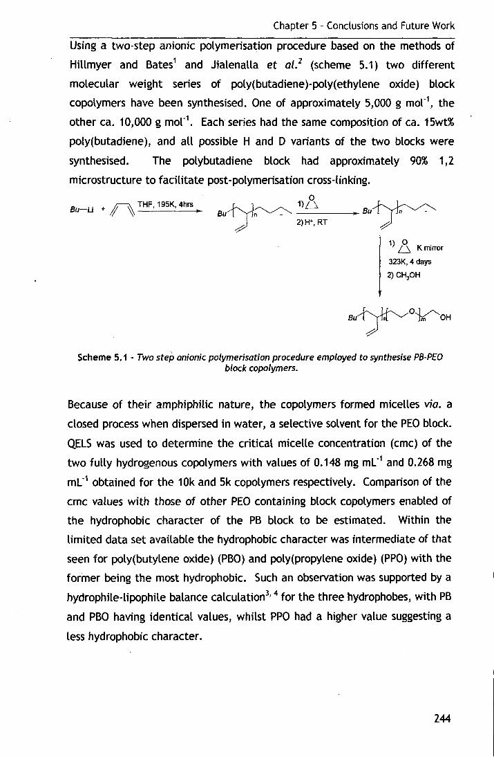
Chapter 5 - Conclusions and Future Work
Using a two-step anionic polymerisation procedure based on the methods of
Hillmyer and Bates 1 and Jialenalla et al. 2 (scheme 5.1) two different
molecular weight series of poly(butadiene)-poly(ethylene oxide) block
copolymers have been synthesised. One of approximately 5,000 g mor1, the
other ea. 10,000 g mor1• Each series had the same composition of ea. 15wt%
poly(butadiene), and all possible H and D variants of the two blocks were
synthesised. The polybutadiene block had approximately 90% 1,2
microstructure to facilitate post-polymerisation cross-linking.
Bu-Li + ~ THF,195K, 4hrs 0
Bu~ -1>_u ___ ._Bu~ ~ 2)H+,RT ~
1) Ji,. K mirror
323K, 4days
2) CH30H
Scheme 5.1 - Two step anionic polymerisation procedure employed to synthesise PB-PEO block copolymers.
Because of their amphiphilic nature, the copolymers formed micelles via. a
closed process when dispersed in water, a selective solvent for the PEO block.
QELS was used to determine the critical micelle concentration (erne) of the
two fully hydrogenous copolymers with values of 0.148 mg ml-1 and 0.268 mg
ml-1 obtained for the 10k and 5k copolymers respectively. Comparison of the
erne values with those of other PEO containing block copolymers enabled of
the hydrophobic character of the PB block to be estimated. Within the
limited data set available the hydrophobic character was intermediate of that
seen for poly(butylene oxide) (PBO) and poly(propylene oxide) (PPO) with the
former being the most hydrophobic. Such an observation was supported by a
hydrophile-lipophile balance calculation3•
4 for the three hydrophobes, with PB
and PBO having identical values, whilst PPO had a higher value suggesting a
less hydrophobic character.
244
Chapter 5 - Conclusions and Future Work
Size determination from QELS experiments revealed hydrodynamic radii of
168A and 1.36A for the 10k and 5k copolymer micelles respectively, which
showed reasonable agreement with Halperin's star model. 5
The quality of the data from SLS and SAXS did not allow size determination of
the micelles, with the lack of contrast and weak scattering intensity from
dilute dispersions in the latter hindering efforts to fit the data.
SANS data from dilute dispersions were successfully fitted to a spherical core
shell model with a parabolic volume fraction profile (as one would expect in a
polymer brush)6 across the micelle corona. The lower molecular weight
micelles had core radii of ea 22A surrounded by a shell thickness of ea BOA,
whilst their higher molecular weight counterparts had core radii of ea 40A and
a shell thickness of ea 11 OA. The two molecular weights exhibited contrasting
association behaviour, with the 5k series having low to moderate association
numbers whilst the 1 Ok series had high association numbers.
In common with the QELS data, reasonable agreement was noted between the
· micelle dimensions and Halperin's star model of micelle formation, but
experimental dimensions were generally larger than those predicted by
theory.
The distance between the PEO junction points on the surface of the core was
less than the calculated unperturbed radius of gyration in all instances, with
the corona chains exhibiting a degree of stretching ea 2.5-4.5 times that of
their unperturbed radius of gyration. These two observations supported the
use of a brush like profile for the corona volume fraction, since they give rise
to the conditions commonly .a.ssociated with a polymer brush. 7• 8
The volume fraction of water in the corona was used to determine the number
of water molecules associated with each ethylene oxide segment. This
revealed that a minimum of six water molecules were associated with each
segment at the core-corona boundary (the driest part of the corona), with this
number increasing with distance from the interface. The number of water
molecules exceeded that associated with hydrated PEO in aqueous solution,
suggesting the conditions inside the polymer brush were highly dilute. 9
Comparison of the corona thickness to theoretical models predicting brush
height showed mixed agreement. The models of Alexander, 7 de Gennes8 and
Milner et al. 6 for planar grafting interfaces provided reasonable agreement
245
Chapter 5 - Conclusions and Future Work
with the experimental values. The model of Dan and Tirrell10 for curved
grafting surfaces provided excellent agreement with the experimental values.
As the concentration of the dispersions was increased, intermicellar
interactions became more prominent. QELS experiments suggested the
presence of particles with dimensions greater than that of the individual
micelles. These larger particles have been attributed to micellar clusters by
others. 11 The 10k micelles formed clusters that were 3-4 times the size of the
micelles whilst the 5k micelles formed clusters that were 6-7 times larger
than the micelles. The difference in the relative dimensions of these clusters
was attributed to the nature of the interactions that appeared to be
operating.
In both SAXS and SANS the presence of a structure factor peak at low Q was
systematic of intermicellar interactions. A hard-sphere potential12"14 could
not describe adequately the observed structure factor and so the mean
spherical approximation of Hayter and Penfold15 was applied. This
reproduced most, but not all, of the features in the SAXS data. In common
with the dilute dispersions, the lack of SAXS contrast made quantitative
determination of interactions difficult. Excellent reproduction of the
structure in the SANS data was however achieved with this model in situations
where the dispersions were still liquid-like in their properties. As the
concentrations were increased to the point where gel formation was
observed, the shape of the scattering changed, with the structure factor peak
moving to higher Q. Under these conditions the MSA could no longer fully
reproduce the features of the data, but reasonable agreement was observed.
The nature of the interactions between the micelles determined from the MSA
agreed well with those determined by McConnell16 and eo-workers using self
consistent field theory. The interaction potentials at low concentrations were
almost hard sphere like in their nature, with a steep rise in potential at low
separations although this was coupled with a slightly softer tail extending to
short separation distances of two to three times the micelle diameter. At
higher concentrations but where the dispersions remained liquid-like, the
interaction potentials rose less steeply at shorter separations, and were
accompanied by a soft tail extending out to relatively long separations of six
246
Chapter 5 - Conclusions and Future Work
to seven times the diameter. The separation distance at which interactions
was observed increased with concentration. Once the dispersions reached the
point where they formed solid gels, the interactions between the micelles
returned to the hard-sphere like potentials observed for the lower
concentrations, but with the rise being steeper and the tail shorter, only
extending to ea 1.5 times the micelle diameter.
Using a redox couple to generate free radicals at room temperature17•
18 it was
possible to cross-link the double bonds of the poly(butadiene) forming the
core of the micelles. The absence of vinyl protons in the NMR spectra was
used to confirm cross-linking. Cross-linked samples of the same isotopic
variants investigated for the virgin micelles were produced.
The use of inorganic salts as a redox couple, and their presence in the
subsequent dispersions complicated the behaviour of the cross-linked micelles
compared to the virgin micelles, due to the reduction in quality of the solvent
for the PEO brush. 19 QELS experiments showed a decrease in the micelle size
upon cross-linking, an observation anticipated both from the expected core
contraction and from published results. The 1 Ok micelles exhibited a
decrease in hydrodynamic radii of ea 7% whilst their 5k counterparts showed a
reduction of ea 30%. Monomodal size distributions in dilute dispersions
confirmed the reaction had been confined to the core of the micelles. Both
molecular weight species exhibited attractive interactions towards one
another, a phenomenon due to remaining inorganic ions after the cross-linking
reaction. Such ions caused a reduction in the thermodynamic quality of the
solvent for the PEO corona re;sulting in interactions between chains being
more favourable than those between chains and the solvent. As for the virgin
micelles the SLS data was not of sufficient quality for determination of
micelle molecular weight or size with confidence.
· SAXS data suggested the micelles had increased in size following the cross
linking reaction, contradicting the observations of the QELS experiments.
However, the inorganic ions are electron rich and as a result increase the
contrast between the different scattering components of the sample.
Consequently, comparison of the micelle dimensions before and after cross-247
Chapter 5 - Conclusions and Future Work
linking is a fruitless exercise due to the vastly different contrast conditions,
which result in more of the micelle being "seen" in the cross-linked
dispersions.
The SANS data from dilute dispersions were successfully fitted using the same
spherical core shell model as for the virgin micelles, suggesting that the
morphology of the micelle remained unchanged upon cross-linking.
Dimensions obtained from these fits showed that both the core radius and
corona thickness had decreased upon cross-linking. The former is due to the
reduction in volume associated with polymerisation of the core, and the latter
is due to the reduced thermodynamic quality of the solvent for the PEO
corona causing the brush to collapse. With one exception, the distance
between the PEO grafting points on the core surface was reduced upon cross
linking. In a good solvent, the fact that the coronal chains come closer
together would be expected to give rise to a thicker corona as the chains
stretch further away from the interface to minimise unfavourable interactions
with one another and maximise favourable interactions with the solvent.
However, in the case here where the solvent may be approaching the theta
condition, interactions between the chains are more favourable than those
with the sol vent.
Surprisingly there was still reasonable agreement between the experimentally
determined micelle dimensions and those predicted by the star model of
Halperin, 5_ even though this was proposed for good solvent conditions. The
model of Dan and Tirrell10 still showed the best agreement for the predicted
brush height, although the relationships of de Gennes8 and Milner et al. 6
showed improved agreement compared to the virgin micelles. This latter
observation is probably a result of the densification of the core upon
polymerisation making the interface between the core and the corona more
rigid and less prone to deformation than in the virgin micelles.
Higher concentration dispersions studied by SAXS exhibited a structure factor
peak that was less pronounced than in the virgin micelles. The mean spherical
approximation was again applied to the data, with more features of the data
captured for the cross-linked micelles than was the case in the virgin
micelles, with the contact potentials between the micelles suggesting a 248

Chapter 5 - Conclusions and Future Work
reduced level of interaction in the cross-linked micelles. As with the dilute
dispersions quantitative comparisons with the virgin micelles was not possible
due to the different contrast conditions between the two sets of dispersions.
In common with the SAXS experiments, the SANS investigations of higher
concentration dispersions also revealed a far less pronounced structure factor
peak. The mean spherical approximation provided excellent fits to the data,
with the contact potentials between micelles also being reduced for a given
molecular weight/concentration combination.
With respect to future work, there are several avenues of research that would
be interesting to explore in the wake of the results presented here.
i.) The micellisation behaviour of PB-PEO block copolymers remains poorly
understood with respect to other PEO containing copolymers. lt would be
interesting to expand the data set of copolymers in terms of the
molecular weights and compositions explored, in order to elucidate the
effect of these variables upon the erne, micelle dimensions and
interactions. The group of Frank Bates have recently explored PB-PEO
block copolymers of varying composition and molecular weight but only in
terms of the morphology of the micelles formed. 20•
21
ii.) lt would likely prove possible to remove the inorganic salts from the
dispersions using a dialysis method, which would enable the cross-linked
micelles to be studied under good solvent conditions, in common with the
virgin micelles.
iii.) The method used to cross-link the micelles could be developed further
such that the micelles can be isolated, separated from the inorganic ions,
and redispersed. This may mean approaching the problem with an
entirely new technique such as photo-initiation with UV light and an
appropriate initiator. Alternatively, a redox couple wherein fewer free
radicals are generated could be used.
iv.) If the cross-linking chemistry could be developed such that the micelles
were redispersible, it would be interesting to study them both in a good
solvent, water, and in a range of solvents with differing affinities for the
PEO, perhaps water at different temperatures, such that the effect of
solvent on the coronal brush could be elucidated. 249

Chapter 5 - Conclusions and Future Work
5.1. Bibliography
2
3
4
5
6
7
8
9
10
11
12
13
14
15
16
17
18
19
20
21
M. A. Hillmyer and F. S. Bates, Macromolecules, 1996, 29, 6994.
G. L. Jialanella, E. M. Firer, and I. Piirma, J Polym Sci, A, Polym
Chem., 1992, 30, 1925.
J. T. Davies and E. K. Rideal, 'Interfacial Phenomena·, 2nd, ed.,
Academic Press, New York, 1963.
R. J. Hunter, 'Foundations of Colloid Science Vol 2', Oxford University
Press, New York, 1989.
A. Halperin, Macromolecules, 1987, 20, 2943.
S. T. Milner, T. A. Witten, and M. E. Cates, Macromolecules, 1988, 21,
2610.
S. Alexander, J. Physique, 19n, 38, 983.
P. G. de Gennes, J. Physique, 1976, 37, 1445.
K. Taskai, J. Am. Chem. Soc., 1996, 118, 8459.
N. Dan and M. Tirrell, Macromolecules, 1992, 25, 2890.
R. L. Xu, et al., Macromolecules, 1991, 24, 87.
N. W. Ashcroft and J. Lekner, Phys. Rev, 1966, 145, 83.
J. K. Perkus and G. J. Yevick, Phys. Rev, 1958, 110, 1.
R. H. Ottewill, in 'Coloidal Dispersions', ed. J. W. Goodwin, Royal
Society of Chemistry, London, 1982.
J. B. Hayter and J. Penfold, Molec. Phys., 1981, 42, 109.
G. A. McConnell, et al., Faraday Discuss., 1994, 98, 121.
Y. Y. Won, H. T. Davis, and F. S. Bates, Science, 1999, 283, 960.
Y. Y. Won, et al., J. Phys. Chem. B, 2001, 105, 8302.
E. Beaudoin, et al., J. Colloid lnterace Sci., 2002, 251, 398.
S. Jain and F. S. Bates, Science, 2003, 300, 460.
Y.Y. Won, et al., J. Phys. Chem. B, 2002, 106, 3354.
250

Appendix A
Appendix A
An analytic structure factor for macroion solutions
S(K) = 1
1- 241Ja(K) where K =Qu
The macroion volume fraction, 11, is expressed in terms of the number
density, n, and the macroion diameter, cr, as:
1lYlCF3 n=--
6
a(K) = A(sinK- K cosK)/ K 3 + B[(2/ K 2 -1)K cosK + 2sinK- 2/ K]l K 3
+ 1JA[24/ K 3 + 4(1- 6/ K 2 )sinK- (1-12/ K 2 + 24/ K 4 )K cosK]/2K 3
+C(kcoshksinK -KsinhkcosK)/ K)l K(K 2 +e)
+ F[ksinhksinK- K(coshkcosK -1]/ K(K 2- k 2
)
+F(cosK -1)/ K 2 -yexp(-k)(ksinK +KcosK)I K(K 2 +e)
where k is the dimensionless screening constant and y is the dimensionless
coupling constant. yexp( -k) is the contact potential for a macroion pair
(expressed in units of KsT).
The coefficients A, B, C and F are expressed in terms of several further sets of
coefficients. For further details the reader is referred to
J.B. Hayter and J. Penfold, Molec. Phys., 1981, 42, 109
251