dwb release notes
DESCRIPTION
Dwb Release NotesTRANSCRIPT

Adobe® Marketing Cloud
Data Workbench Release Notes
Contents
Data Workbench Release Notes......................................................................................3Data Workbench 6.4 Release Notes............................................................................................................................3
Exporting to Analytics Core Services....................................................................................................................................................8
Workstation Setup Wizard ....................................................................................................................................................................10
Presentation Layer....................................................................................................................................................................................14
Metric Dim Wizard....................................................................................................................................................................................16
User Administration of Group Member Access.............................................................................................................................19
Locking Profiles in the Workstation...................................................................................................................................................23
Localizing Time Dimensions.................................................................................................................................................................23
New User Interface Features.................................................................................................................................................................26
Device Atlas with In-Memory Cache..................................................................................................................................................26
Data Workbench 6.31 Update....................................................................................................................................27
Data Workbench 6.3 Release Notes..........................................................................................................................28
Data Workbench 6.3 features...............................................................................................................................................................36
Data Workbench 6.21 Update....................................................................................................................................64
Data Workbench 6.2 Release Notes..........................................................................................................................66
Data Workbench 6.2 features...............................................................................................................................................................68
Data Workbench 6.11 Update....................................................................................................................................98
Data Feeds Update for April MR 2014......................................................................................................................99
Data Workbench 6.1 Release Notes.......................................................................................................................111
Data Workbench 6.1 features.............................................................................................................................................................112
Data Workbench 5.5 to 6.1 Upgrade...............................................................................................................................................125
Data Workbench 6.0 to 6.1 Upgrade...............................................................................................................................................128
Data Workbench 6.0 Release Notes.......................................................................................................................131
Data Workbench 6.0 Release Notes.................................................................................................................................................132
Data Workbench 6.0 features.............................................................................................................................................................136
Data Workbench 6.0.4 Release Notes.............................................................................................................................................157
Data Workbench Release NotesLast updated 6/25/2015
Data Workbench Release NotesIdentify new features, upgrade instructions, and bug fixes for released versions of Data Workbench.
Data Workbench 6.4 Release Notes
Data Workbench 6.4 release notes include new features, upgrade requirements, fixed bugs, and known issues.
To view previous features and fixes for past releases, see the release notes archive.
New Features
Upgrade Requirements
System Updates
Fixed Bugs
Known Issues
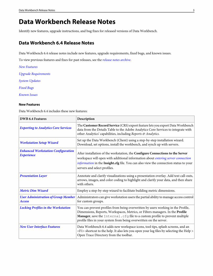
New Features
Data Workbench 6.4 includes these new features:
DescriptionDWB 6.4 Features
The Customer Record Service (CRS) export feature lets you export Data Workbenchdata from the Details Table to the Adobe Analytics Core Services to integrate withother Analytics' capabilities, including Reports & Analytics.
Exporting to Analytics Core Services
Set up the Data Workbench (Client) using a step-by-step installation wizard.Download, set options, install the workbench, and synch up with servers.Workstation Setup Wizard
After installation of the workstation, the Configure Connections to the Serverworkspace will open with additional information about entering server connection
Enhanced Workstation ConfigurationExperience
information in the Insight.cfg file. You can also view the connection status to yourservers and select profiles.
Annotate and clarify visualizations using a presentation overlay. Add text call-outs,arrows, images, and color coding to highlight and clarify your data, and then sharewith others.
Presentation Layer
Employ a step-by-step wizard to facilitate building metric dimensions.Metric Dim Wizard
Administrators can give workstation users the partial ability to manage access controlfor custom groups.
User Administration of Group MemberAccess
You can prevent profiles from being overwritten by users working in the Profile,Dimensions, Reports, Workspaces, Metrics, or Filters managers. In the Profile
Locking Profiles in the Workstation
Manager, save the Internal.cfg file to a custom profile to prevent multipleprofile files in your system from being overwritten on the server.
Data Workbench 6.4 adds new workspace icons, tool tips, splash screens, and an<F1> shortcut to the help. It also lets you open your log files by selecting the Help >Open Trace Directory from the toolbar.
New User Interface Features
3Data Workbench Release Notes
DescriptionDWB 6.4 Features
Expectation Maximization added to Clustering feature.
This is an Adobe Analytics Premium feature.
Updated Clustering algorithm
Data workbench now uses an expanded logging framework "L4" which provides theability to configure logging based on the need. The default implementation that comes
Updated Logging information
with the 6.4 package provides vital information on the software processing. Loggingcan be expanded with additional information to troubleshoot server events and helpanalyze underlying issues, including additional information for associated server,client and report server.
For additional support in implementing additional L4 logging, please contact youraccount manager.
A new httpLoggingEI.cfg configuration file (located atserver\Admin\Export\httpLoggingEI.cfg) lets you stop INFO logging
New cfg file for ExportIntegration.exelogging options
to the HTTP.log file during Export Integration exports. (The CRS, TNT, and MMPexports already capture verbose logging in individual export log files.)
A true setting starts INFO logging (for testing and detailed reporting) to theHTTP.log file, and a false setting stops verbose logging. For a false setting, only aWARNING/ERROR level messages will be sent to the HTTP.log file.
Use the zoom feature to better view metric labels when values reach a higher disparity.Previously the label would disappear with the change in the contrast of values-for
Zoom feature for Graph visualizations
example, when you set a higher metric regression value against previous values. Youcan now zoom in to the visualization by clicking <Ctrl> and moving the mouse wheelwhile hovering over the graph.
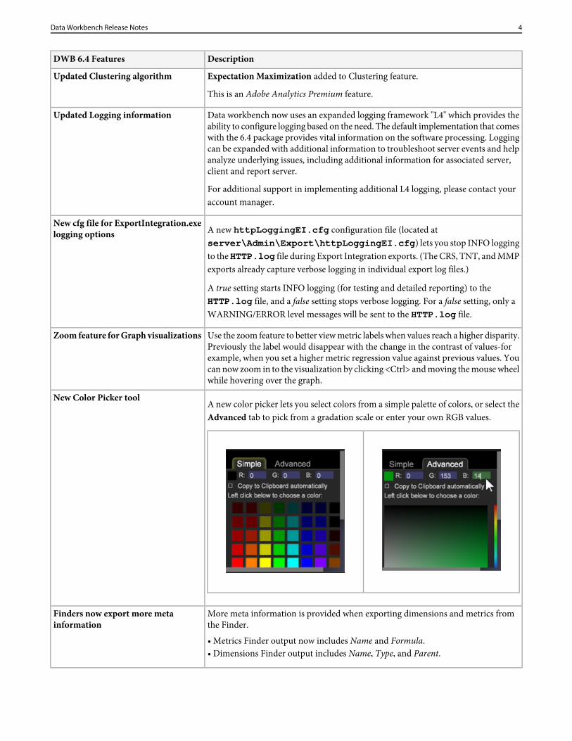
A new color picker lets you select colors from a simple palette of colors, or select theAdvanced tab to pick from a gradation scale or enter your own RGB values.
New Color Picker tool
More meta information is provided when exporting dimensions and metrics fromthe Finder.
Finders now export more metainformation
• Metrics Finder output now includes Name and Formula.• Dimensions Finder output includes Name, Type, and Parent.
4Data Workbench Release Notes
DescriptionDWB 6.4 Features
These executables are now digitally signed to ensure that the software downloadshave not been altered or corrupted.
Insight.exe and InsightSetup.exe arenow digitally signed.
You can change the date format based on your locale in the Standard TimeDimensions.cfg file. Change the default MM/DD/YYYY format to theDD/MM/YYYY format or choose other options.
Date format options
The Files visualization ( Admin > Files) for Base profiles will not include largerdirectories (removed Logs, Exports, and Lookups) when reporting. This will increasethe speed in displaying the report.
Files visualization broken out
The larger directories now have their own individual reports ( Admin / Export Files,Lookup Files and Log Files).
The DeviceAtlas.bundle file now uses in-memory cache to greatly improve theperformance of look-ups.
Device Atlas with In-Memory Cache
Improved visibility when hovering over a section when viewing the Chordvisualization.
Updated Chord visualization
From the workstation, you can now drag dimensions from Finder panel directly tothe Detail Table in a workspace.
Drag dimensions from Finder to aDetail Table
Upgrade Requirements
Follow these requirements and recommendations when upgrading to Data Workbench 6.4.
Important: It is recommended that you use the newly installed default configuration files and customize them, rather thanmoving files from a previous installation—with these exceptions:
• Add Excluded Processes for MS System Center Endpoint Protection in Windows 2012 Servers for the following executables:
• InsightServer64.exe• ReportServer.exe• ExportIntegration.exe
This will allow "white list" rights for these interfacing executables.
• Update the Trust_ca_cert.pem certificate on the servers.• Reorganization of Attribution Profiles.
• The Attribution folder was renamed to Attribution - Premium (found in the default installation at Profiles\Attribution -Premium).
• The Premium profile was removed and the workspace moved to the new Attribution - Premium folder.
• Update Attribution-Premium settings. If you have customized profiles with parameter settings that override the default AdobeSC profile, then you need to update the custom fields in these configuration files:
• Decoding Instructions.cfg
• SC Fields.cfg
• Because of this reorganization, you will want to remove the old Attribution and Premium folders from your server installation.
Change these settingsProfile = profileInfo: Active = bool: true
5Data Workbench Release Notes
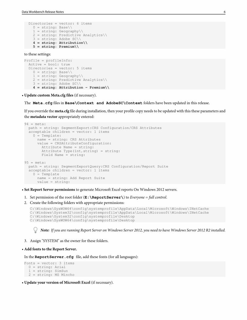
Directories = vector: 6 items 0 = string: Base\\ 1 = string: Geography\\ 2 = string: Predictive Analytics\\ 3 = string: Adobe SC\\
4 = string: Attribution\\ 5 = string: Premium\\
to these settings:Profile = profileInfo: Active = bool: true Directories = vector: 5 items 0 = string: Base\\ 1 = string: Geography\\ 2 = string: Predictive Analytics\\ 3 = string: Adobe SC\\
4 = string: Attribution - Premium\\
• Update custom Meta.cfg files (if necessary).
The Meta.cfg files in Base\Context and AdobeSC\Context folders have been updated in this release.
If you override the meta.cfg file during installation, then your profile copy needs to be updated with this these parameters andthe metadata vector appropriately entered:
94 = meta: path = string: SegmentExport:CRS Configuration/CRS Attributes acceptable children = vector: 1 items 0 = Template: name = string: CRS Attributes value = CRSAttributeConfiguration: Attribute Name = string: Attribute Type(int,string) = string: Field Name = string:
95 = meta: path = string: SegmentExportQuery:CRS Configuration/Report Suite acceptable children = vector: 1 items 0 = Template name = string: Add Report Suite value = string:
• Set Report Server permissions to generate Microsoft Excel reports On Windows 2012 servers.
1. Set permission of the root folder (E:\ReportServer\) to Everyone = full control.2. Create the following folders with appropriate permissions:
C:\Windows\SysWOW64\config\systemprofile\AppData\Local\Microsoft\Windows\INetCacheC:\Windows\System32\config\systemprofile\AppData\Local\Microsoft\Windows\INetCacheC:\Windows\System32\config\systemprofile\DesktopC:\Windows\SysWOW64\config\systemprofile\Desktop
Note: If you are running Report Server on Windows Server 2012, you need to have Windows Server 2012 R2 installed.
3. Assign "SYSTEM" as the owner for these folders.
• Add fonts to the Report Server.
In the ReportServer.cfg file, add these fonts (for all languages):Fonts = vector: 3 items 0 = string: Arial 1 = string: SimSun 2 = string: MS Mincho
• Update your version of Microsoft Excel (if necessary).
6Data Workbench Release Notes
With the release of Data Workbench 6.4, support for Excel 2007 has been discontinued. Also because Data Workbench onlyruns on Microsoft Windows for 64-bit architecture, it is recommended that you also install a 64-bit version of Microsoft Excel.
• 64-bit architecture required for Workstation (Client) installation.• Run the Workstation Setup Wizard.
Install the new version of the workstation (client) by downloading and launching InsightSetup.exe and stepping through thesetup instructions. The setup wizard will install your files to a new location by default:
Program files are now saved by default to:C:\Program Files\Adobe\Adobe Analytics\Data Workbench
Data Files (profiles, certificates, trace logs, and user files) are now saved by default to:C:\Users\<username>\AppData\Local\Adobe\Adobe Analytics\Data Workbench\
• Add fonts to the Workstation.
In the Insight.cfg file, add these fonts (for all languages):Fonts = vector: 3 items 0 = string: Arial 1 = string: SimSun 2 = string: MS Mincho
System Updates
These features have been renamed, deleted, or the installation files or folders were restructured in this release:
• The Base.zip folder is no longer included in the version update package.• The DeviceAtlas.bundle file now uses an in-memory cache to improve the performance of lookups.• In the Log Processing.cfg file, the Chunk Size parameter under Log Sources was removed.• In the Segment Export.cfg file, the Segment Export Destination parameter was removed.• In the Disk Files.cfg file, the Detect Disk Corruption parameter was removed in these locations:
\server\components\disk files.cfg
\server\components for processing servers\disk files.cfg
• New service descriptions for Adobe Analytics Premium Services and for Adobe Analytics Premium Report Services in theexecutable properties.
• The Master Marketing Profile Export feature in the Details Table was renamed to Profiles & Audiences Export.• The Test and Target Export feature in the Details Table was renamed to Adobe Target Export.
Fixed Bugs
The following fixes were made in Data Workbench 6.4 (since the release of Data Workbench 6.31).
• Propensity score wasn't resetting when rerunning different inputs in the same workspace. This now resets properly.• No countable dimensions available when first opening the Correlation Matrix has been fixed.• Export of Target segments were failing because the mboxPC field was missing. This is now fixed.• ID request formatted correctly. Using the mbox3rdpartyId identification instead of default PCIDs caused Adobe Target to
reject requests generated via the Target/Data Workbench integration (using the ExportIntegration.exe). This IDrequest is now being formatted correctly and throughput is successful.
• Report Server memory leak when exporting to Excel has been fixed.
7Data Workbench Release Notes
Known Issues
The following are known restrictions in Data Workbench 6.4.
• ExportIntegration.exe requires command-line arguments in English. The output file name should be named in Englishfor Adobe Target Export, Profiles and Audiences Export, and Customer Record Service Export.
• In the Profiles and Audience Export, entering unauthorized characters ([CR] or [TAB]) as column names generates incorrectlogs resulting in data not exporting correctly.
• In Chinese and Japanese versions, Unicode character encoding issue might be encountered in the Path Browser.
Additional Data Workbench Documentation online
Exporting to Analytics Core Services
The Customer Record Service (CRS) export feature lets you export Data Workbench data to the Adobe Analytics Core Servicesto integrate with other Analytics' capabilities, including Reports & Analytics.
From a Detail Table (right-click Tools > Detail Table in a workspace), you can set attribute values and the variablesrequired to integrate with Analytics' Reports & Analytics (using Adobe Pipeline Services).
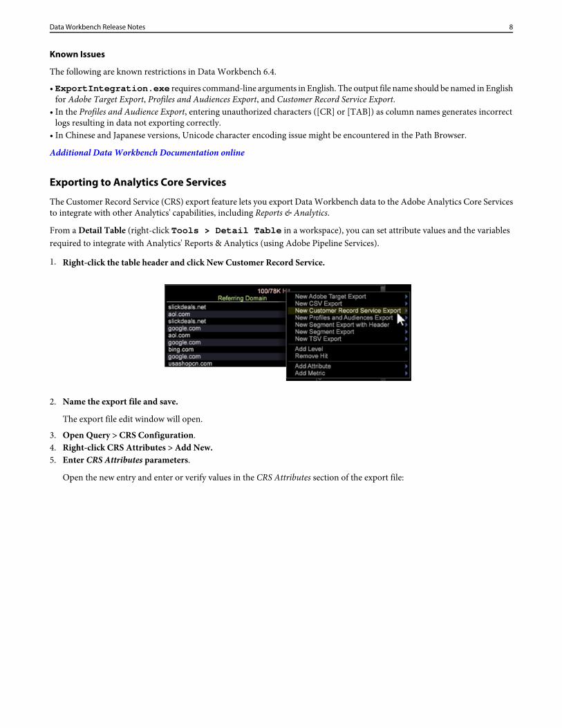
1. Right-click the table header and click New Customer Record Service.
2. Name the export file and save.
The export file edit window will open.
3. Open Query > CRS Configuration.4. Right-click CRS Attributes > Add New.5. Enter CRS Attributes parameters.
Open the new entry and enter or verify values in the CRS Attributes section of the export file:
8Data Workbench Release Notes
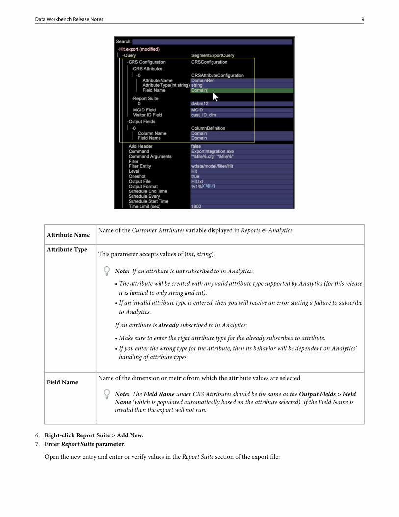
Name of the Customer Attributes variable displayed in Reports & Analytics.Attribute Name
This parameter accepts values of (int, string).Attribute Type
Note: If an attribute is not subscribed to in Analytics:
• The attribute will be created with any valid attribute type supported by Analytics (for this releaseit is limited to only string and int).
• If an invalid attribute type is entered, then you will receive an error stating a failure to subscribeto Analytics.
If an attribute is already subscribed to in Analytics:
• Make sure to enter the right attribute type for the already subscribed to attribute.• If you enter the wrong type for the attribute, then its behavior will be dependent on Analytics'
handling of attribute types.
Name of the dimension or metric from which the attribute values are selected.Field Name
Note: The Field Name under CRS Attributes should be the same as the Output Fields > FieldName (which is populated automatically based on the attribute selected). If the Field Name isinvalid then the export will not run.
6. Right-click Report Suite > Add New.7. Enter Report Suite parameter.
Open the new entry and enter or verify values in the Report Suite section of the export file:
9Data Workbench Release Notes
Name of the report suite in Reports & Analytics identifying the Customer Attribute variables beingexported.
Report Suite
Note: Although Reports & Analytics lets you add to multiple report suites, Data Workbench 6.4will only export a single report suite identified at index 0.
The report suite name entered in this field is the report suite ID (and not the name of the reportsuite).
8. Enter MCID Field parameter.
Name of the dimension in your profile that represents the Adobe Marketing Cloud ID. This is a mandatoryfield and any invalid dimension value entered will not export.
MCID field
9. (optional) Enter Visitor ID Field parameter.
If the user wishes to send any other custom ID for a visitor in his/her data, this is where they enter thename of the dimension which represents the custom visitor id. This is an optional field an can be leftempty.
Visitor ID Field
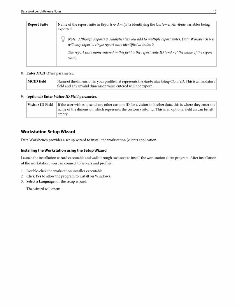
Workstation Setup Wizard
Data Workbench provides a set up wizard to install the workstation (client) application.
Installing the Workstation using the Setup Wizard
Launch the installation wizard executable and walk through each step to install the workstation client program. After installationof the workstation, you can connect to servers and profiles.
1. Double-click the workstation installer executable.2. Click Yes to allow the program to install on Windows.3. Select a Language for the setup wizard.
The wizard will open:
10Data Workbench Release Notes
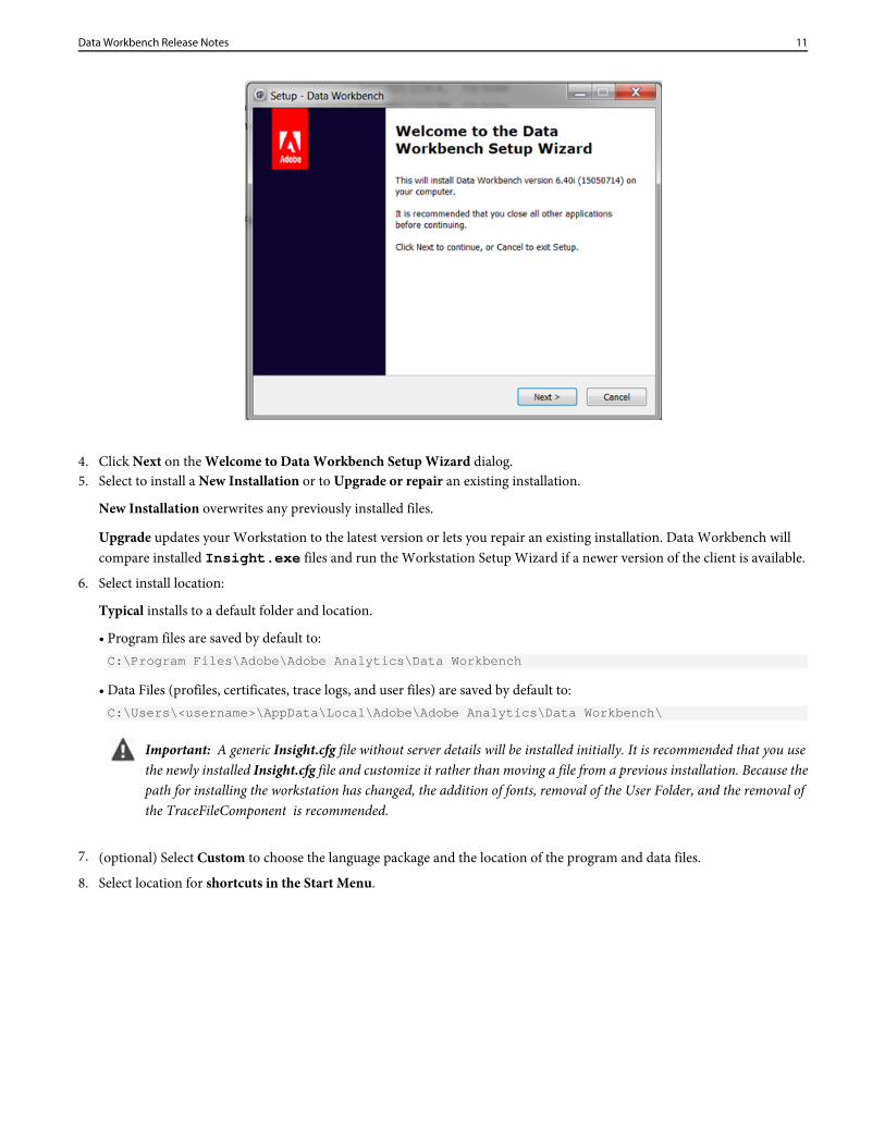
4. Click Next on the Welcome to Data Workbench Setup Wizard dialog.5. Select to install a New Installation or to Upgrade or repair an existing installation.
New Installation overwrites any previously installed files.
Upgrade updates your Workstation to the latest version or lets you repair an existing installation. Data Workbench willcompare installed Insight.exe files and run the Workstation Setup Wizard if a newer version of the client is available.
6. Select install location:
Typical installs to a default folder and location.
• Program files are saved by default to:C:\Program Files\Adobe\Adobe Analytics\Data Workbench
• Data Files (profiles, certificates, trace logs, and user files) are saved by default to:C:\Users\<username>\AppData\Local\Adobe\Adobe Analytics\Data Workbench\
Important: A generic Insight.cfg file without server details will be installed initially. It is recommended that you usethe newly installed Insight.cfg file and customize it rather than moving a file from a previous installation. Because thepath for installing the workstation has changed, the addition of fonts, removal of the User Folder, and the removal ofthe TraceFileComponent is recommended.
7. (optional) Select Custom to choose the language package and the location of the program and data files.
8. Select location for shortcuts in the Start Menu.
11Data Workbench Release Notes
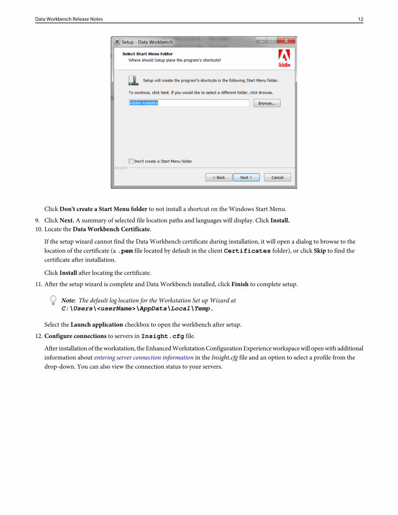
Click Don't create a Start Menu folder to not install a shortcut on the Windows Start Menu.
9. Click Next. A summary of selected file location paths and languages will display. Click Install.10. Locate the Data Workbench Certificate.
If the setup wizard cannot find the Data Workbench certificate during installation, it will open a dialog to browse to thelocation of the certificate (a .pem file located by default in the client Certificates folder), or click Skip to find thecertificate after installation.
Click Install after locating the certificate.
11. After the setup wizard is complete and Data Workbench installed, click Finish to complete setup.
Note: The default log location for the Workstation Set up Wizard atC:\Users\<userName>\AppData\Local\Temp.
Select the Launch application checkbox to open the workbench after setup.
12. Configure connections to servers in Insight.cfg file.
After installation of the workstation, the Enhanced Workstation Configuration Experience workspace will open with additionalinformation about entering server connection information in the Insight.cfg file and an option to select a profile from thedrop-down. You can also view the connection status to your servers.
12Data Workbench Release Notes
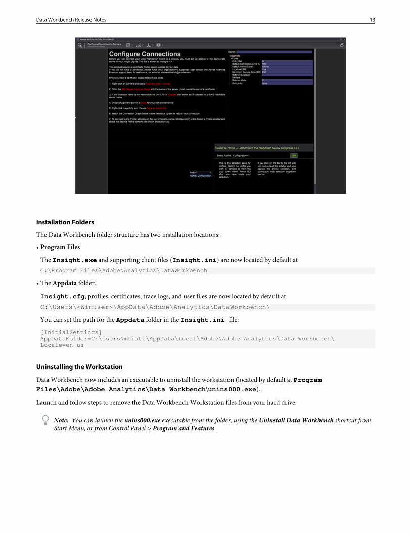
Installation Folders
The Data Workbench folder structure has two installation locations:
• Program Files
The Insight.exe and supporting client files (Insight.ini) are now located by default atC:\Program Files\Adobe\Analytics\DataWorkbench
• The Appdata folder.
Insight.cfg, profiles, certificates, trace logs, and user files are now located by default atC:\Users\<Winuser>\AppData\Adobe\Analytics\DataWorkbench\
You can set the path for the Appdata folder in the Insight.ini file:
[InitialSettings]AppDataFolder=C:\Users\mhiatt\AppData\Local\Adobe\Adobe Analytics\Data Workbench\Locale=en-us
Uninstalling the Workstation
Data Workbench now includes an executable to uninstall the workstation (located by default at ProgramFiles\Adobe\Adobe Analytics\Data Workbench\unins000.exe).
Launch and follow steps to remove the Data Workbench Workstation files from your hard drive.
Note: You can launch the unins000.exe executable from the folder, using the Uninstall Data Workbench shortcut fromStart Menu, or from Control Panel > Program and Features.
13Data Workbench Release Notes
Presentation Layer
The Presentation Layer lets you mark up and annotate your workspace visualizations and then publish with your call-outs andcomments. Add text descriptions, graphic objects, callout arrows, color coding, images, and other features in an overlay to addannotations and clarify important data points, and then share with stakeholders.
Add Annotations to your Visualizations:
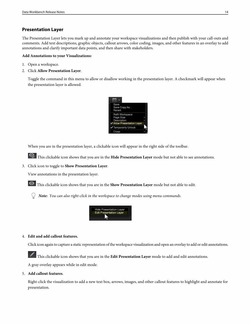
1. Open a workspace.2. Click Allow Presentation Layer.
Toggle the command in this menu to allow or disallow working in the presentation layer. A checkmark will appear whenthe presentation layer is allowed.
When you are in the presentation layer, a clickable icon will appear in the right side of the toolbar.
This clickable icon shows that you are in the Hide Presentation Layer mode but not able to see annotations.
3. Click icon to toggle to Show Presentation Layer.
View annotations in the presentation layer.
This clickable icon shows that you are in the Show Presentation Layer mode but not able to edit.
Note: You can also right-click in the workspace to change modes using menu commands.
4. Edit and add callout features.
Click icon again to capture a static representation of the workspace visualization and open an overlay to add or edit annotations.
This clickable icon shows that you are in the Edit Presentation Layer mode to add and edit annotations.
A gray overlay appears while in edit mode.
5. Add callout features.
Right-click the visualization to add a new text box, arrows, images, and other callout features to highlight and annotate forpresentation.
14Data Workbench Release Notes
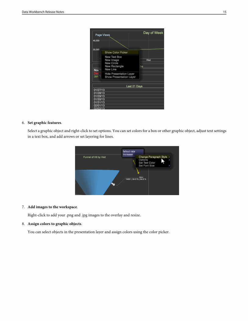
6. Set graphic features.
Select a graphic object and right-click to set options. You can set colors for a box or other graphic object, adjust text settingsin a text box, and add arrows or set layering for lines.
7. Add images to the workspace.
Right-click to add your .png and .jpg images to the overlay and resize.
8. Assign colors to graphic objects.
You can select objects in the presentation layer and assign colors using the color picker.
15Data Workbench Release Notes
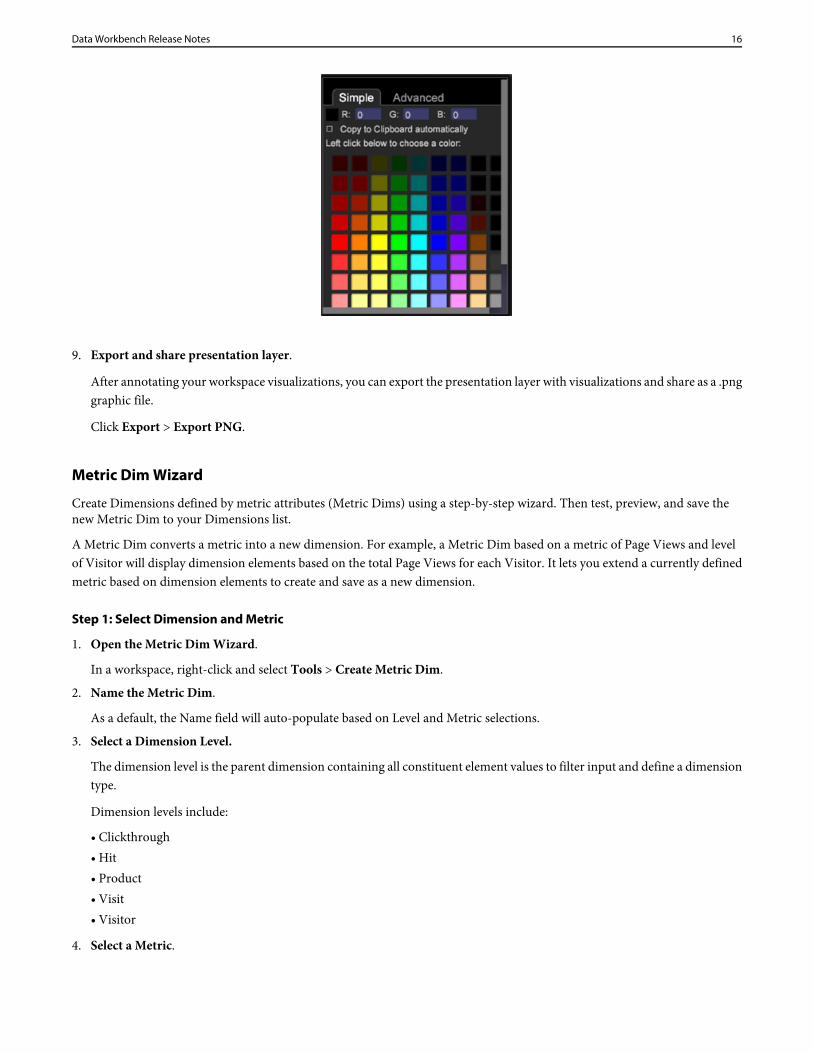
9. Export and share presentation layer.
After annotating your workspace visualizations, you can export the presentation layer with visualizations and share as a .pnggraphic file.
Click Export > Export PNG.
Metric Dim Wizard
Create Dimensions defined by metric attributes (Metric Dims) using a step-by-step wizard. Then test, preview, and save thenew Metric Dim to your Dimensions list.
A Metric Dim converts a metric into a new dimension. For example, a Metric Dim based on a metric of Page Views and levelof Visitor will display dimension elements based on the total Page Views for each Visitor. It lets you extend a currently definedmetric based on dimension elements to create and save as a new dimension.
Step 1: Select Dimension and Metric
1. Open the Metric Dim Wizard.
In a workspace, right-click and select Tools > Create Metric Dim.
2. Name the Metric Dim.
As a default, the Name field will auto-populate based on Level and Metric selections.
3. Select a Dimension Level.
The dimension level is the parent dimension containing all constituent element values to filter input and define a dimensiontype.
Dimension levels include:
• Clickthrough• Hit• Product• Visit• Visitor
4. Select a Metric.
16Data Workbench Release Notes
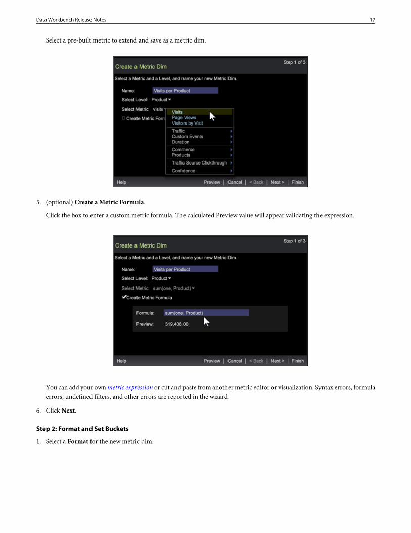
Select a pre-built metric to extend and save as a metric dim.
5. (optional) Create a Metric Formula.
Click the box to enter a custom metric formula. The calculated Preview value will appear validating the expression.
You can add your own metric expression or cut and paste from another metric editor or visualization. Syntax errors, formulaerrors, undefined filters, and other errors are reported in the wizard.
6. Click Next.
Step 2: Format and Set Buckets
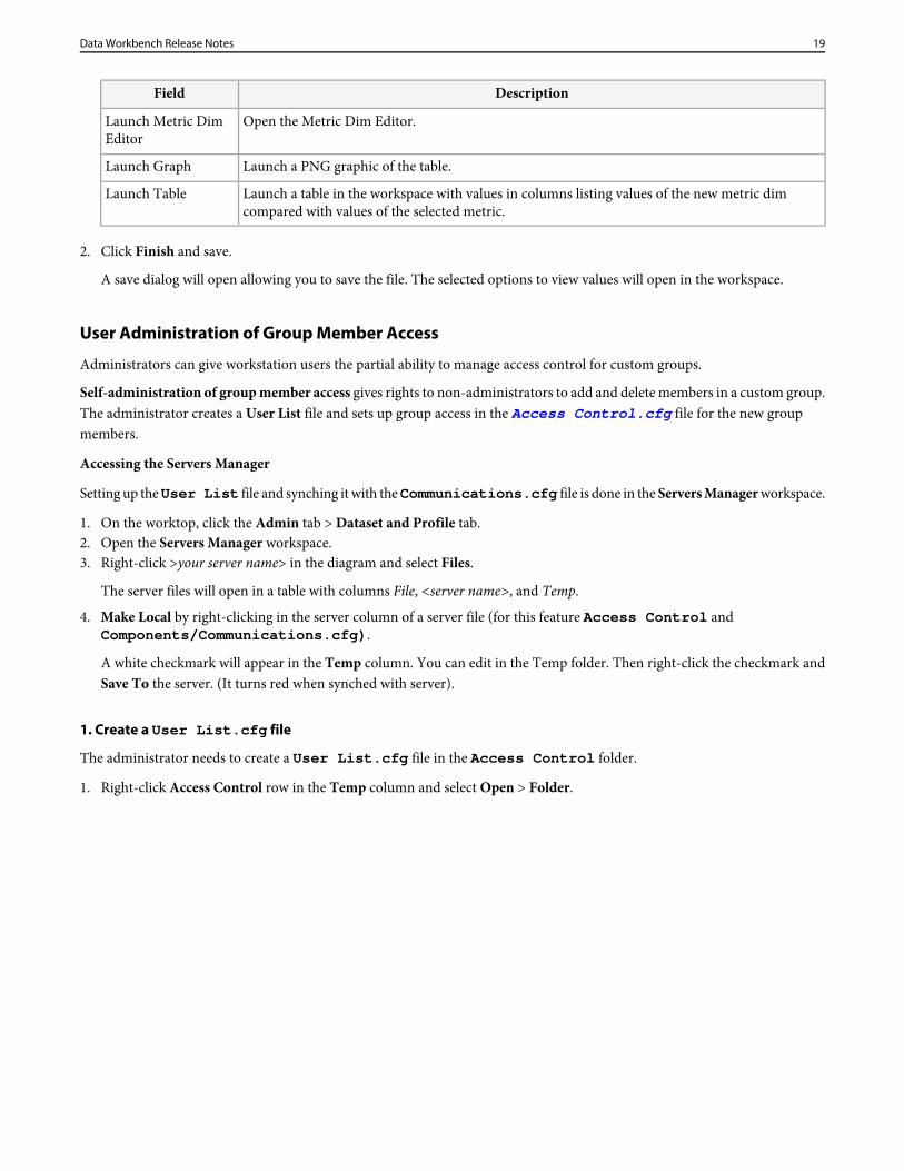
1. Select a Format for the new metric dim.
17Data Workbench Release Notes
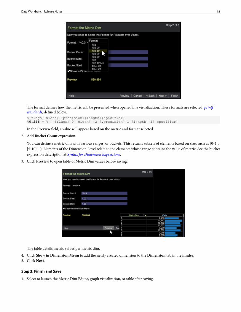
The format defines how the metric will be presented when opened in a visualization. These formats are selected printfstandards, defined below:%[flags][width][.precision][length][specifier]%0.2lf = % _ [flags] 0 [width] .2 [.precision] l [length] f[ specifier]
In the Preview field, a value will appear based on the metric and format selected.
2. Add Bucket Count expression.
You can define a metric dim with various ranges, or buckets. This returns subsets of elements based on size, such as [0-4],[5-10],...). Elements of the Dimension Level relate to the elements whose range contains the value of metric. See the bucketexpression description at Syntax for Dimension Expressions.
3. Click Preview to open table of Metric Dim values before saving.
The table details metric values per metric dim.
4. Click Show in Dimension Menu to add the newly created dimension to the Dimension tab in the Finder.5. Click Next.
Step 3: Finish and Save
1. Select to launch the Metric Dim Editor, graph visualization, or table after saving.
18Data Workbench Release Notes
DescriptionField
Open the Metric Dim Editor.Launch Metric DimEditor
Launch a PNG graphic of the table.Launch Graph
Launch a table in the workspace with values in columns listing values of the new metric dimcompared with values of the selected metric.
Launch Table
2. Click Finish and save.
A save dialog will open allowing you to save the file. The selected options to view values will open in the workspace.
User Administration of Group Member Access
Administrators can give workstation users the partial ability to manage access control for custom groups.
Self-administration of group member access gives rights to non-administrators to add and delete members in a custom group.The administrator creates a User List file and sets up group access in the Access Control.cfg file for the new groupmembers.
Accessing the Servers Manager
Setting up the User List file and synching it with the Communications.cfg file is done in the Servers Manager workspace.
1. On the worktop, click the Admin tab > Dataset and Profile tab.2. Open the Servers Manager workspace.3. Right-click >your server name> in the diagram and select Files.
The server files will open in a table with columns File, <server name>, and Temp.
4. Make Local by right-clicking in the server column of a server file (for this feature Access Control andComponents/Communications.cfg).
A white checkmark will appear in the Temp column. You can edit in the Temp folder. Then right-click the checkmark andSave To the server. (It turns red when synched with server).
1. Create a User List.cfg file
The administrator needs to create a User List.cfg file in the Access Control folder.
1. Right-click Access Control row in the Temp column and select Open > Folder.
19Data Workbench Release Notes
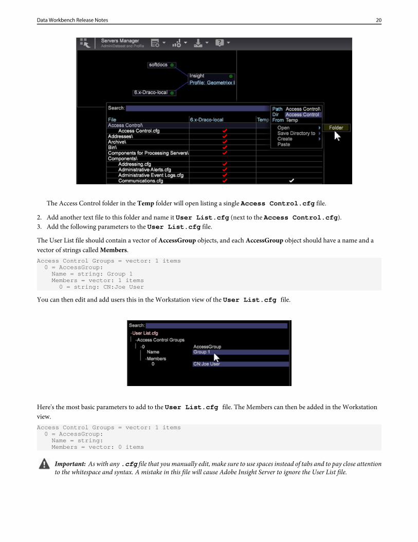
The Access Control folder in the Temp folder will open listing a single Access Control.cfg file.
2. Add another text file to this folder and name it User List.cfg (next to the Access Control.cfg).3. Add the following parameters to the User List.cfg file.
The User List file should contain a vector of AccessGroup objects, and each AccessGroup object should have a name and avector of strings called Members.Access Control Groups = vector: 1 items 0 = AccessGroup: Name = string: Group 1 Members = vector: 1 items 0 = string: CN:Joe User
You can then edit and add users this in the Workstation view of the User List.cfg file.
Here's the most basic parameters to add to the User List.cfg file. The Members can then be added in the Workstationview.Access Control Groups = vector: 1 items 0 = AccessGroup: Name = string: Members = vector: 0 items
Important: As with any .cfg file that you manually edit, make sure to use spaces instead of tabs and to pay close attentionto the whitespace and syntax. A mistake in this file will cause Adobe Insight Server to ignore the User List file.
20Data Workbench Release Notes
The Name field in each Access Group will be referenced within the Access Control.cfg file.
Note: Only valid members with directory service prefixes, such as CN: or OU: are accepted, and these cannot containwildcard character (*).
2. Set up the Communications.cfg file
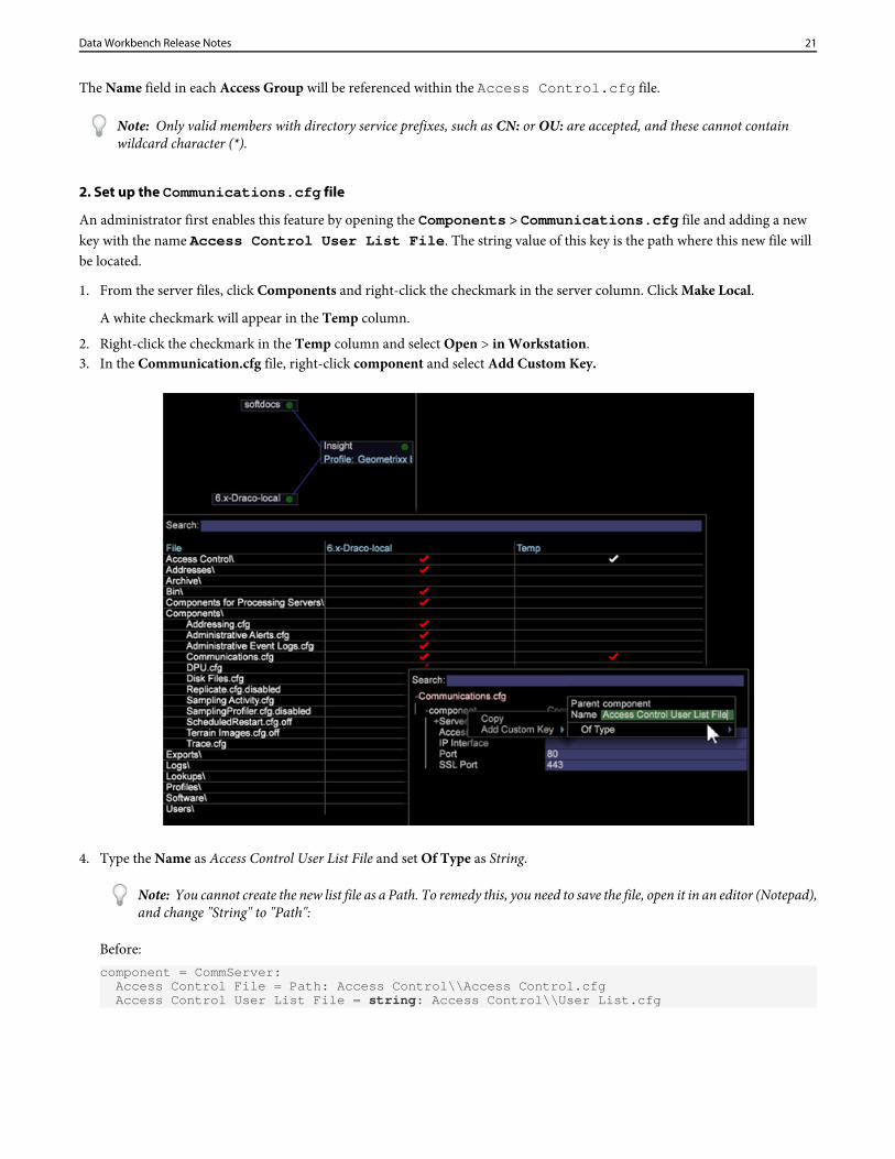
An administrator first enables this feature by opening the Components > Communications.cfg file and adding a newkey with the name Access Control User List File. The string value of this key is the path where this new file willbe located.
1. From the server files, click Components and right-click the checkmark in the server column. Click Make Local.
A white checkmark will appear in the Temp column.
2. Right-click the checkmark in the Temp column and select Open > in Workstation.3. In the Communication.cfg file, right-click component and select Add Custom Key.
4. Type the Name as Access Control User List File and set Of Type as String.
Note: You cannot create the new list file as a Path. To remedy this, you need to save the file, open it in an editor (Notepad),and change "String" to "Path":
Before:component = CommServer: Access Control File = Path: Access Control\\Access Control.cfg Access Control User List File = string: Access Control\\User List.cfg
21Data Workbench Release Notes
After:component = CommServer: Access Control File = Path: Access Control\\Access Control.cfg Access Control User List File = Path: Access Control\\User List.cfg
5. Save the Communications.cfg file and (if necessary) save it to the server. This will restart components in the server tomake sure you haven't made any mistakes that could prevent the Communications.cfg file from being parsed.
6. If your system includes processing servers, modify the configuration file in the Components for ProcessingServers.cfg file.
7. Right-click Communications.cfg and save to server.
The Data Workbench administrator can now confirm that the intended user(s) have access to the user list file and allow theusers to manage the group. The user(s) will be able to open the User List file, edit it, and add and remove CN or OU membersas needed.
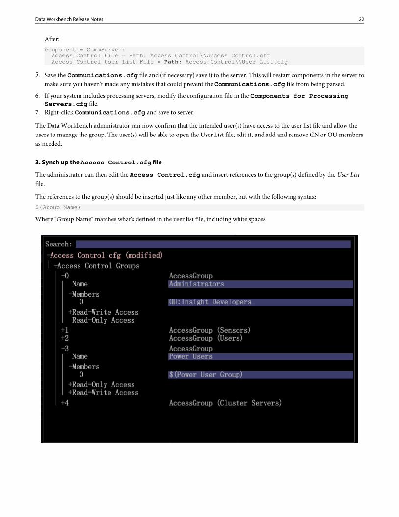
3. Synch up the Access Control.cfg file
The administrator can then edit the Access Control.cfg and insert references to the group(s) defined by the User Listfile.
The references to the group(s) should be inserted just like any other member, but with the following syntax:$(Group Name)
Where "Group Name" matches what's defined in the user list file, including white spaces.
22Data Workbench Release Notes
At this point the Data Workbench administrator can confirm that select group users have access to the user list file. The selectusers can then open the User List.cfg file, edit it, and add and remove CN or OU members as needed.
Locking Profiles in the Workstation
The Internal.cfg file applied in the Profile Manager prevents changes by users to your custom profiles by the Profile,Dimensions, Reports, Workspaces, Metrics, and Filters managers.
You can prevent profile files from being modified and overwritten when using the managers by saving the Internal.cfgfile to your custom profile in the Profile Manager. This configuration file prevents users from overwriting multiple files whenworking in the managers (accessed from the Admin > Profile menu).
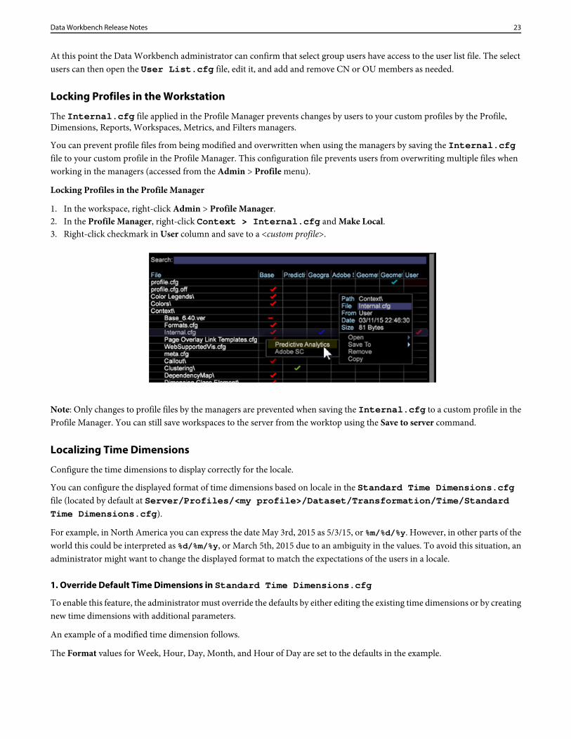
Locking Profiles in the Profile Manager
1. In the workspace, right-click Admin > Profile Manager.2. In the Profile Manager, right-click Context > Internal.cfg and Make Local.3. Right-click checkmark in User column and save to a <custom profile>.
Note: Only changes to profile files by the managers are prevented when saving the Internal.cfg to a custom profile in theProfile Manager. You can still save workspaces to the server from the worktop using the Save to server command.
Localizing Time Dimensions
Configure the time dimensions to display correctly for the locale.
You can configure the displayed format of time dimensions based on locale in the Standard Time Dimensions.cfgfile (located by default at Server/Profiles/<my profile>/Dataset/Transformation/Time/StandardTime Dimensions.cfg).
For example, in North America you can express the date May 3rd, 2015 as 5/3/15, or %m/%d/%y. However, in other parts of theworld this could be interpreted as %d/%m/%y, or March 5th, 2015 due to an ambiguity in the values. To avoid this situation, anadministrator might want to change the displayed format to match the expectations of the users in a locale.
1. Override Default Time Dimensions in Standard Time Dimensions.cfg
To enable this feature, the administrator must override the defaults by either editing the existing time dimensions or by creatingnew time dimensions with additional parameters.
An example of a modified time dimension follows.
The Format values for Week, Hour, Day, Month, and Hour of Day are set to the defaults in the example.
23Data Workbench Release Notes
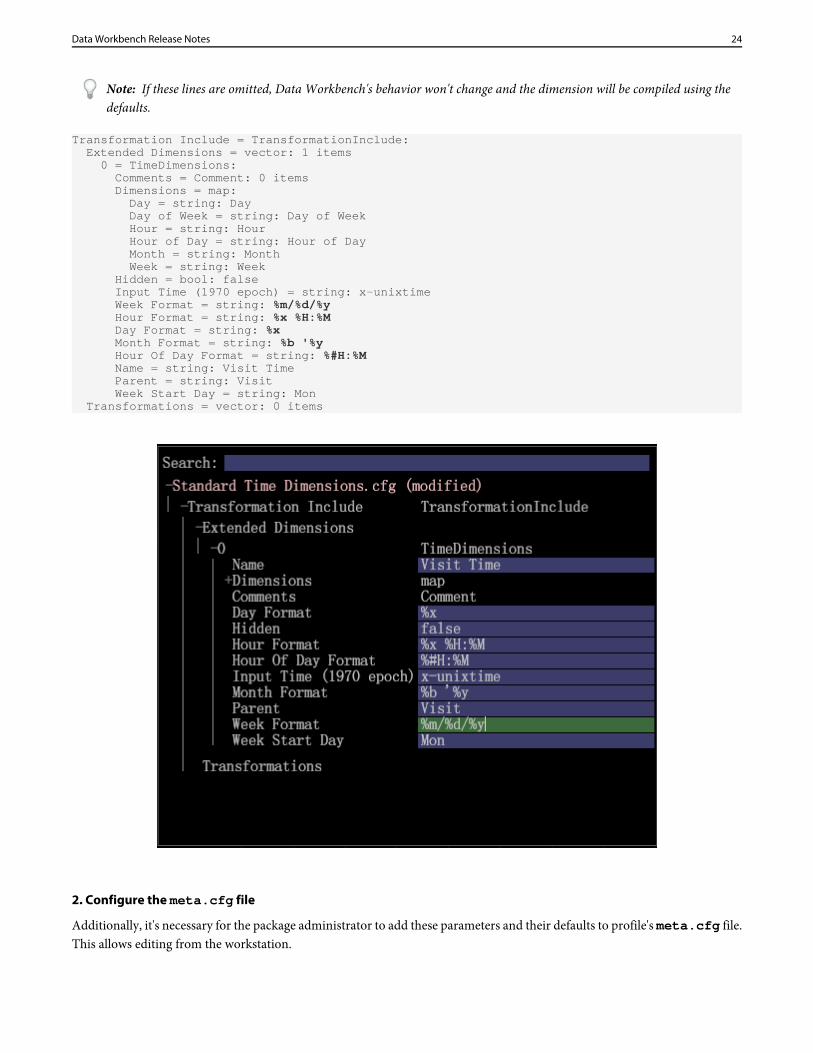
Note: If these lines are omitted, Data Workbench's behavior won't change and the dimension will be compiled using thedefaults.
Transformation Include = TransformationInclude: Extended Dimensions = vector: 1 items 0 = TimeDimensions: Comments = Comment: 0 items Dimensions = map: Day = string: Day Day of Week = string: Day of Week Hour = string: Hour Hour of Day = string: Hour of Day Month = string: Month Week = string: Week Hidden = bool: false Input Time (1970 epoch) = string: x-unixtime Week Format = string: %m/%d/%y Hour Format = string: %x %H:%M Day Format = string: %x Month Format = string: %b '%y Hour Of Day Format = string: %#H:%M Name = string: Visit Time Parent = string: Visit Week Start Day = string: Mon Transformations = vector: 0 items
2. Configure the meta.cfg file
Additionally, it's necessary for the package administrator to add these parameters and their defaults to profile's meta.cfg file.This allows editing from the workstation.
24Data Workbench Release Notes
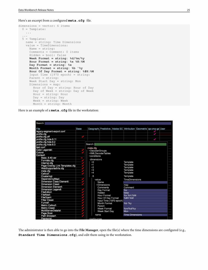
Here's an excerpt from a configured meta.cfg file.dimensions = vector: 6 items 0 = Template: ... ... 5 = Template: name = string: Time Dimensions value = TimeDimensions: Name = string: Comments = Comment: 0 items Hidden = bool: false
Week Format = string: %d/%m/%y Hour Format = string: %x %H:%M Day Format = string: %x Month Format = string: %b '%y Hour Of Day Format = string: %#H:%M Input Time (1970 epoch) = string: Parent = string: Week Start Day = string: Mon Dimensions = map: Hour of Day = string: Hour of Day Day of Week = string: Day of Week Hour = string: Hour Day = string: Day Week = string: Week Month = string: Month
Here is an example of a meta.cfg file in the workstation:
The administrator is then able to go into the File Manager, open the file(s) where the time dimensions are configured (e.g.,Standard Time Dimensions.cfg), and edit them using in the workstation.
25Data Workbench Release Notes
New User Interface Features
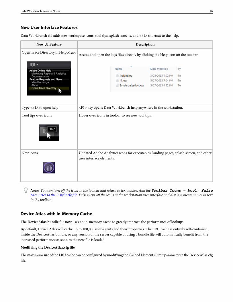
Data Workbench 6.4 adds new workspace icons, tool tips, splash screens, and <F1> shortcut to the help.
DescriptionNew UI Feature
Access and open the logs files directly by clicking the Help icon on the toolbar .Open Trace Directory in Help Menu
<F1> key opens Data Workbench help anywhere in the workstation.Type <F1> to open help
Hover over icons in toolbar to see new tool tips.Tool tips over icons
Updated Adobe Analytics icons for executables, landing pages, splash screen, and otheruser interface elements.
New icons
Note: You can turn off the icons in the toolbar and return to text names. Add the Toolbar Icons = bool: falseparameter to the Insight.cfg file. False turns off the icons in the workstation user interface and displays menu names in textin the toolbar.
Device Atlas with In-Memory Cache
The DeviceAtlas.bundle file now uses an in-memory cache to greatly improve the performance of lookups
By default, Device Atlas will cache up to 100,000 user-agents and their properties. The LRU cache is entirely self-containedinside the DeviceAtlas.bundle, so any version of the server capable of using a bundle file will automatically benefit from theincreased performance as soon as the new file is loaded.
Modifying the DeviceAtlas.cfg file
The maximum size of the LRU cache can be configured by modifying the Cached Elements Limit parameter in the DeviceAtlas.cfgfile.
26Data Workbench Release Notes
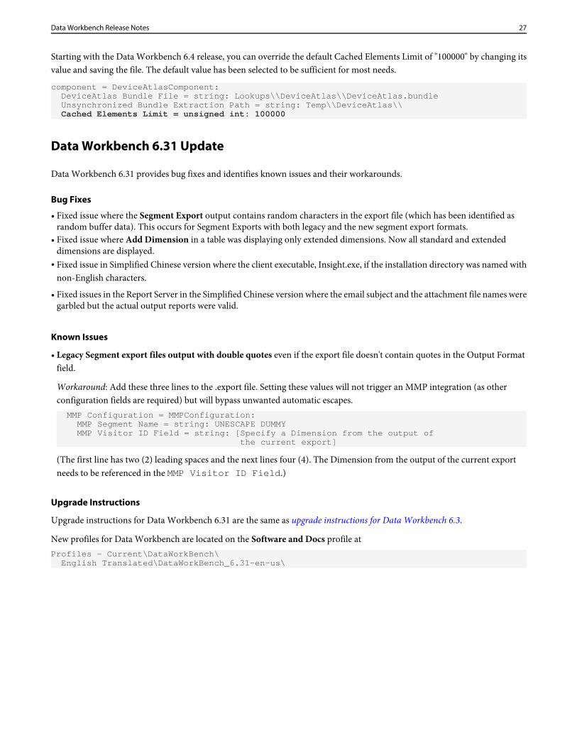
Starting with the Data Workbench 6.4 release, you can override the default Cached Elements Limit of "100000" by changing itsvalue and saving the file. The default value has been selected to be sufficient for most needs.
component = DeviceAtlasComponent: DeviceAtlas Bundle File = string: Lookups\\DeviceAtlas\\DeviceAtlas.bundle Unsynchronized Bundle Extraction Path = string: Temp\\DeviceAtlas\\ Cached Elements Limit = unsigned int: 100000
Data Workbench 6.31 Update
Data Workbench 6.31 provides bug fixes and identifies known issues and their workarounds.
Bug Fixes
• Fixed issue where the Segment Export output contains random characters in the export file (which has been identified asrandom buffer data). This occurs for Segment Exports with both legacy and the new segment export formats.
• Fixed issue where Add Dimension in a table was displaying only extended dimensions. Now all standard and extendeddimensions are displayed.
• Fixed issue in Simplified Chinese version where the client executable, Insight.exe, if the installation directory was named withnon-English characters.
• Fixed issues in the Report Server in the Simplified Chinese version where the email subject and the attachment file names weregarbled but the actual output reports were valid.
Known Issues
• Legacy Segment export files output with double quotes even if the export file doesn't contain quotes in the Output Formatfield.
Workaround: Add these three lines to the .export file. Setting these values will not trigger an MMP integration (as otherconfiguration fields are required) but will bypass unwanted automatic escapes. MMP Configuration = MMPConfiguration: MMP Segment Name = string: UNESCAPE DUMMY MMP Visitor ID Field = string: [Specify a Dimension from the output of the current export]
(The first line has two (2) leading spaces and the next lines four (4). The Dimension from the output of the current exportneeds to be referenced in the MMP Visitor ID Field.)
Upgrade Instructions
Upgrade instructions for Data Workbench 6.31 are the same as upgrade instructions for Data Workbench 6.3.
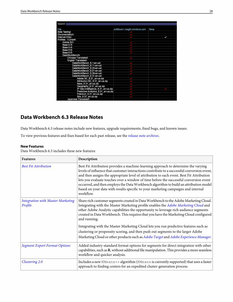
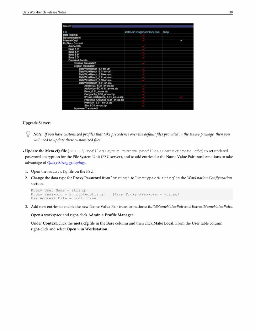
New profiles for Data Workbench are located on the Software and Docs profile atProfiles - Current\DataWorkBench\ English Translated\DataWorkBench_6.31-en-us\
27Data Workbench Release Notes
Data Workbench 6.3 Release Notes
Data Workbench 6.3 release notes include new features, upgrade requirements, fixed bugs, and known issues.
To view previous features and fixes based for each past release, see the release note archives.
New FeaturesData Workbench 6.3 includes these new features:
DescriptionFeatures
Best Fit Attribution provides a machine-learning approach to determine the varyinglevels of influence that customer interactions contribute to a successful conversion event,
Best Fit Attribution
and then assigns the appropriate level of attribution to each event. Best Fit Attributionlets you evaluate touches over a window of time before the successful conversion eventoccurred, and then employs the Data Workbench algorithm to build an attribution modelbased on your data with results specific to your marketing campaigns and internalworkflow.
Share rich customer segments created in Data Workbench to the Adobe Marketing Cloud.Integrating with the Master Marketing profile enables the Adobe Marketing Cloud and
Integration with Master MarketingProfile
other Adobe Analytic capabilities the opportunity to leverage rich audience segmentscreated in Data Workbench. This requires that you have the Marketing Cloud configuredand running.
Integrating with the Master Marketing Cloud lets you run predictive features such asclustering or propensity scoring, and then push out segments to the larger AdobeMarketing Cloud or other products such as Adobe Target and Adobe Experience Manager.
Added industry-standard format options for segments for direct integration with othercapabilities, such as R, without additional file manipulation. This provides a more seamlessworkflow and quicker analysis.
Segment Export Format Options
Includes a new KMeans++ algorithm (KMeans is currently supported) that uses a fasterapproach to finding centers for an expedited cluster-generation process.
Clustering 2.0
28Data Workbench Release Notes
DescriptionFeatures
Present a very visual and easy-to-interpret depiction of the data.Trend Lines
Provides the ability to compare the impact of one factor to another directly within theanalyst workflow.
Regression Analysis graph
Updates to the Pie Chart visualization lets you use default colors identified in a legend,or set colors based on the color chart.
Pie Chart update
The Chord Visualization provides another view of the Correlation Matrix.Chord Visualization
If you have many fields with custom evars, props, and variables, during log processingyou can build a name value pair to combine fields in a report.
Query String Grouping
The Latency visualization lets you analyze latent customer behavior within a set numberof days before or after an event occurred after a campaign or other event type.
Latency Analysis
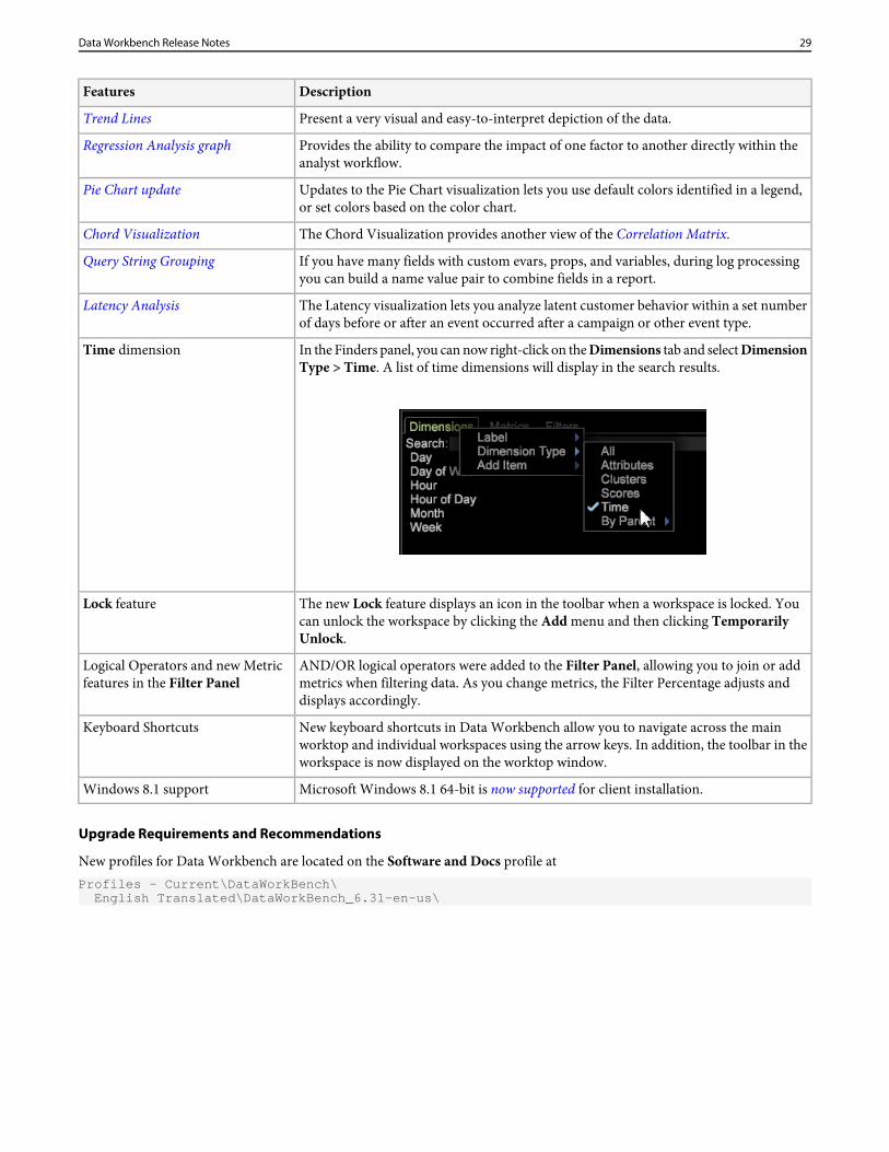
In the Finders panel, you can now right-click on the Dimensions tab and select DimensionType > Time. A list of time dimensions will display in the search results.
Time dimension
The new Lock feature displays an icon in the toolbar when a workspace is locked. Youcan unlock the workspace by clicking the Add menu and then clicking TemporarilyUnlock.
Lock feature
AND/OR logical operators were added to the Filter Panel, allowing you to join or addmetrics when filtering data. As you change metrics, the Filter Percentage adjusts anddisplays accordingly.
Logical Operators and new Metricfeatures in the Filter Panel
New keyboard shortcuts in Data Workbench allow you to navigate across the mainworktop and individual workspaces using the arrow keys. In addition, the toolbar in theworkspace is now displayed on the worktop window.
Keyboard Shortcuts
Microsoft Windows 8.1 64-bit is now supported for client installation.Windows 8.1 support
Upgrade Requirements and Recommendations
New profiles for Data Workbench are located on the Software and Docs profile atProfiles - Current\DataWorkBench\ English Translated\DataWorkBench_6.31-en-us\
29Data Workbench Release Notes
Upgrade Server:
Note: If you have customized profiles that take precedence over the default files provided in the Base package, then youwill need to update these customized files:
• Update the Meta.cfg file (E:\..\Profiles\<your custom profile>\Context\meta.cfg)to set updatedpassword encryption for the File System Unit (FSU server), and to add entries for the Name Value Pair tranformations to takeadvantage of Query String groupings.
1. Open the meta.cfg file on the FSU.2. Change the data type for Proxy Password from "string" to "EncryptedString" in the Workstation Configuration
section.Proxy User Name = string:Proxy Password = EncryptedString: (from Proxy Password = String)Use Address File = bool: true
3. Add new entries to enable the new Name Value Pair transformations: BuildNameValuePair and ExtractNameValuePairs.
Open a workspace and right-click Admin > Profile Manager.
Under Context, click the meta.cfg file in the Base column and then click Make Local. From the User table column,right-click and select Open > in Workstation.
30Data Workbench Release Notes
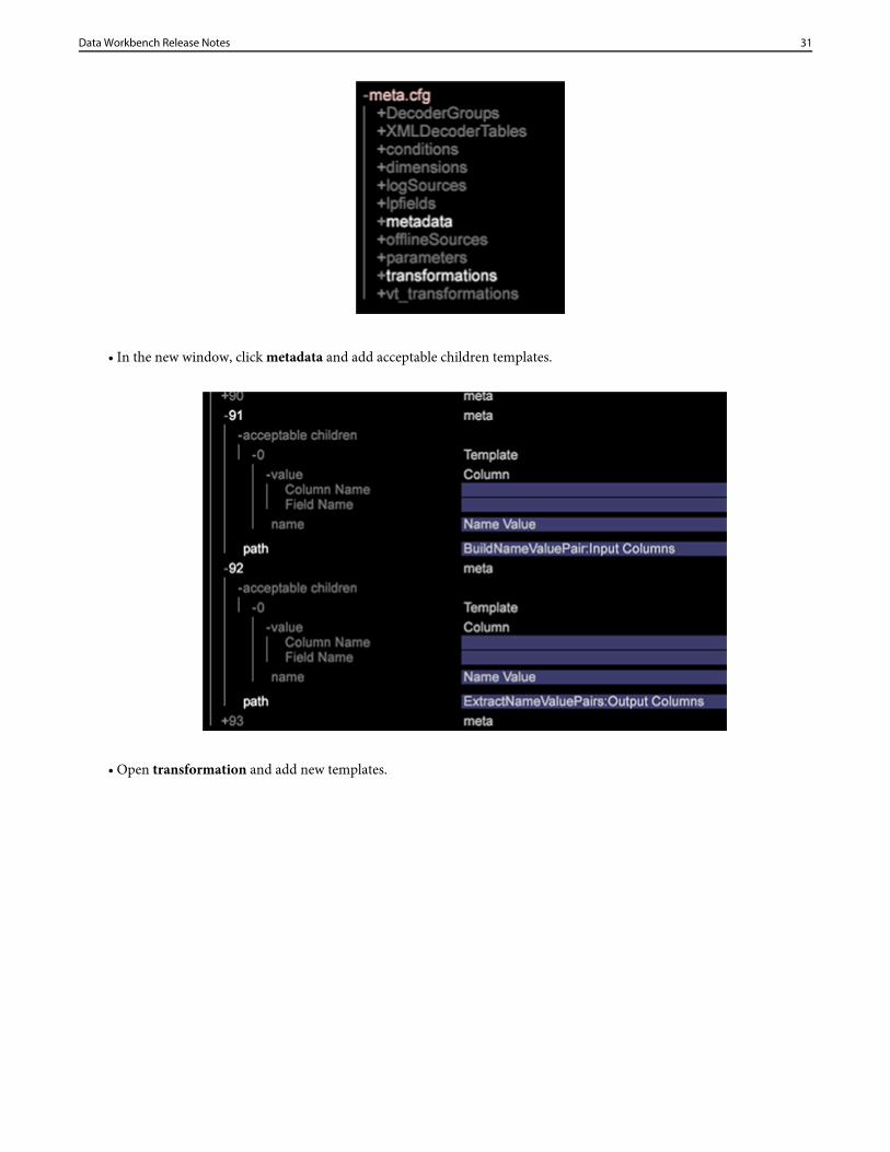
• In the new window, click metadata and add acceptable children templates.
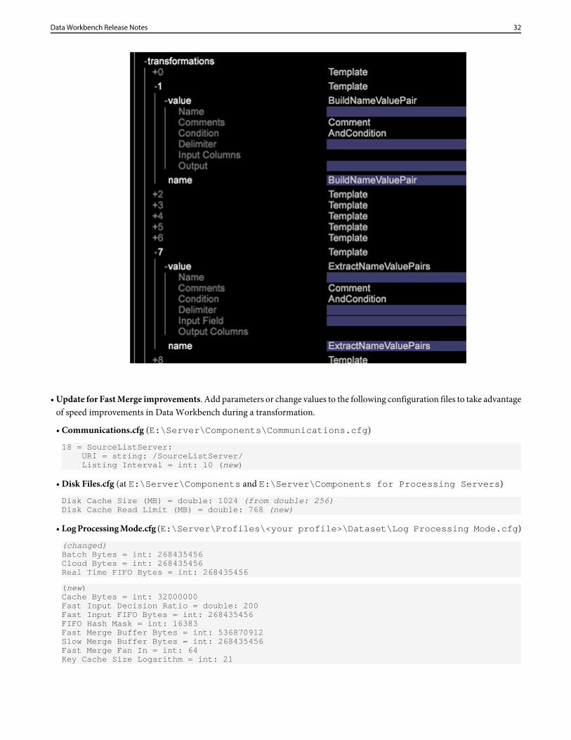
• Open transformation and add new templates.
31Data Workbench Release Notes
• Update for Fast Merge improvements. Add parameters or change values to the following configuration files to take advantageof speed improvements in Data Workbench during a transformation.
• Communications.cfg (E:\Server\Components\Communications.cfg)
18 = SourceListServer: URI = string: /SourceListServer/ Listing Interval = int: 10 (new)
• Disk Files.cfg (at E:\Server\Components and E:\Server\Components for Processing Servers)
Disk Cache Size (MB) = double: 1024 (from double: 256)Disk Cache Read Limit (MB) = double: 768 (new)
• Log Processing Mode.cfg (E:\Server\Profiles\<your profile>\Dataset\Log Processing Mode.cfg)
(changed)Batch Bytes = int: 268435456Cloud Bytes = int: 268435456Real Time FIFO Bytes = int: 268435456
(new)Cache Bytes = int: 32000000Fast Input Decision Ratio = double: 200Fast Input FIFO Bytes = int: 268435456FIFO Hash Mask = int: 16383Fast Merge Buffer Bytes = int: 536870912Slow Merge Buffer Bytes = int: 268435456Fast Merge Fan In = int: 64Key Cache Size Logarithm = int: 21
32Data Workbench Release Notes
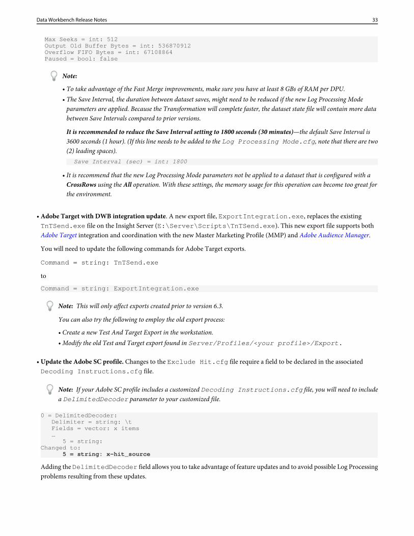
Max Seeks = int: 512Output Old Buffer Bytes = int: 536870912Overflow FIFO Bytes = int: 67108864Paused = bool: false
Note:
• To take advantage of the Fast Merge improvements, make sure you have at least 8 GBs of RAM per DPU.• The Save Interval, the duration between dataset saves, might need to be reduced if the new Log Processing Mode
parameters are applied. Because the Transformation will complete faster, the dataset state file will contain more databetween Save Intervals compared to prior versions.
It is recommended to reduce the Save Interval setting to 1800 seconds (30 minutes)—the default Save Interval is3600 seconds (1 hour). (If this line needs to be added to the Log Processing Mode.cfg, note that there are two(2) leading spaces). Save Interval (sec) = int: 1800
• It is recommend that the new Log Processing Mode parameters not be applied to a dataset that is configured with aCrossRows using the All operation. With these settings, the memory usage for this operation can become too great forthe environment.
• Adobe Target with DWB integration update. A new export file, ExportIntegration.exe, replaces the existingTnTSend.exe file on the Insight Server (E:\Server\Scripts\TnTSend.exe). This new export file supports bothAdobe Target integration and coordination with the new Master Marketing Profile (MMP) and Adobe Audience Manager.
You will need to update the following commands for Adobe Target exports.
Command = string: TnTSend.exe
to
Command = string: ExportIntegration.exe
Note: This will only affect exports created prior to version 6.3.
You can also try the following to employ the old export process:
• Create a new Test And Target Export in the workstation.• Modify the old Test and Target export found in Server/Profiles/<your profile>/Export.
• Update the Adobe SC profile. Changes to the Exclude Hit.cfg file require a field to be declared in the associatedDecoding Instructions.cfg file.
Note: If your Adobe SC profile includes a customized Decoding Instructions.cfg file, you will need to includea DelimitedDecoder parameter to your customized file.
0 = DelimitedDecoder: Delimiter = string: \t Fields = vector: x items … 5 = string:Changed to:
5 = string: x-hit_source
Adding the DelimitedDecoder field allows you to take advantage of feature updates and to avoid possible Log Processingproblems resulting from these updates.
33Data Workbench Release Notes
Upgrade Client:
•• Update your client from the server.
Once your server has been updated, your client can update automatically if the Insight.cfg file is configured properly:
1. Edit the Insight.cfg file.Update Software = bool: true
Then Save.
2. Exit and launch the client.
3. Connect to the profile.
The client will automatically upgrade to Data Workbench 6.3.
4. Exit out of the client.5. Edit Insight.cfg
• Change Proxy Password = string:
to Proxy Password = EncryptedString:
Remove the value of the previous Proxy Address and Proxy Password.
• Save.
6. Launch the client.7. Edit Insight.cfg.
• Enter Proxy Password for all the servers and Save.• Enter the Proxy Address for all the servers and Save.
Important: The Proxy Address and Proxy Password must be entered and saved from within the client.
8. Connect to the profile.
Note:
• Follow the exact upgrade sequence in order to avoid an account lockout. If the account is locked, please perform all therequired changes in the exact sequence listed, save your work, and exit out of the client. Wait for the lockout to release(about 45 minutes), then launch the client again.
• The password modification should be performed in the client only due to the fact that the passwords are saved in WindowsCredential Vault.
• Recommendation: New Windows Aero Themes.
Upgrade the look of your client application using Windows Aero Themes.
• Recommendation: Fonts for Chinese and Japanese versions:
Chinese:
• Arial• SimSun
34Data Workbench Release Notes
Japanese:
• MS Gothic• Meiryo• MS Mincho• Arial• SimSun
Note: SimSun can be used for Chinese and Japanese. If attempting to write in half-byte characters in Japanese, you alsoneed to include MS Mincho. To enable these fonts in Insight.cfg, you can add these parameters.
0 = string: Arial1 = string: SimSun2 = string: MS Mincho
These fonts should be listed in the workstation configuration file: Insight.cfg.
Upgrade to Adobe Analytics Premium
To run Best Fit Attribution in Data Workbench, you need to receive new certificates from Adobe ClientCare for your Client,Server, and Report Server (.pem files) to support Adobe Analytics Premium. Each of the new certificates will have this parameter:Product = Premium
The Premium Package is available for download on Software and Docs under the Getting Started tab on the Profiles andLookup files workspace. Navigate to Profiles - Current\DataWorkBench\<language>\DataWorkBench_6.30-en-us\Premium_6.30_en-us.zip.
Once the Premium profile is loaded on your Server, you will need to add a Premium parameter to your custom Profile.cfgfile. This allows your custom profile to include the menus, visualizations, and workspaces as part of Adobe Analytics Premium.
Fixed Bugs
• Fixed issue where the Density Map visualization was missing largest elements.• Fixed issue in Density Map where area of elements was not portraying the proportion of the metric value.• Fixed issue where dragging metric from Finders panel to metric legend outside of the metric column would delete the legend
from the workspace.• Fixed issue where Print Workspace using Sidebar and Both options will not include the Copyright info in the printed page.
Known Issues
• Users of AMD Radeon™ graphics cards should update to the latest graphics drivers. Some early versions of the driver claimthey support openGL 3.2 but are inconsistent.
• Output generated by Segment Export configuration without a header declaration can result in a bogus header appearing atthe beginning of the file that conflicts with the first set of rows.
• Add Dimensions is showing only the Extended Dimensions. The workaround is to use the Finders tool to drag dimensionsto tables.
• When 3D Scatter Plot Visualization includes callouts, the zoom might display plots outside the border of the visualization. Towork around this issue, zoom the 3D Scatter Plot first and then add callouts to your visualization.
• Using Workstation in Remote Desktop session will crash when renaming workspaces.•• Legacy Segment export files output with double quotes even if the export file doesn't contain quotes in the Output Format
field.
35Data Workbench Release Notes
Workaround: Add these three lines to the .export file. Setting these values will not trigger an MMP integration (as otherconfiguration fields are required) but will bypass unwanted automatic escapes. MMP Configuration = MMPConfiguration: MMP Segment Name = string: UNESCAPE DUMMY MMP Visitor ID Field = string: [Specify a Dimension from the output of the current export]
(The first line has two (2) leading spaces and the next lines four (4). The Dimension from the output of the current exportneeds to be referenced in the MMP Visitor ID Field.)
Data Workbench 6.3 features
Data Workbench 6.3 includes the following features.
Best Fit Attribution
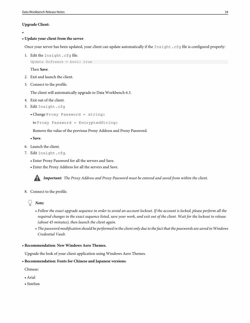
Best Fit Attribution is a machine-learning approach to assigning attribution values across the different channels of a successfulconversion event. Data Workbench automatically evaluates contributions to success across a window of time per channel, andthen builds an attribution model based on your customers' actual interaction patterns.
Best Fit Attribution lets you compare the interactions, or touches, that contributed to a successful sale, email sign-up, or otherperformance indicators. The attribution analysis automatically assigns weight to the most important touches and provides anattribution model per channel based on your data and responsive to your market and internal protocols.
For example, if a customer visits your site through an organic search, then engages with a campaign, and then signs up for anemail, rules-based Attribution would identify the first touch or last touch, or evenly distribute success attribution across all touchpoints using preset attribution models. Where rules-based attribution is defined by the user, the Best Fit attributes sets valuesthrough an algorithm by calculating the probability of a conversion as a function of the observed touch points.
36Data Workbench Release Notes
Note: To run Best Fit Attribution in Data Workbench, you need to update your server certificate (.pem file) to supportAdobe Analytics Premium. You also need to add Premium to your custom Profile.cfg for the client and receive newcertificates from Adobe ClientCare for Server and Report Server. See upgrade instructions for Data Workbench 6.3.
Basic Setup
See Build a Best Fit Attribution for step-by-step instructions.
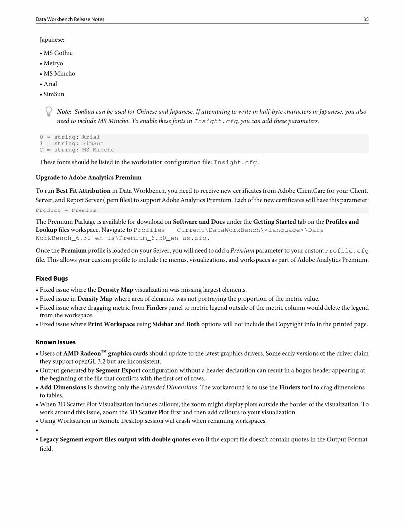
Set the Success metricDefine a metric representing a success event.
The Success Metric is often Orders, although you can leverage Data Workbench to define a very complicated success metric inconjunction with the Success Window.
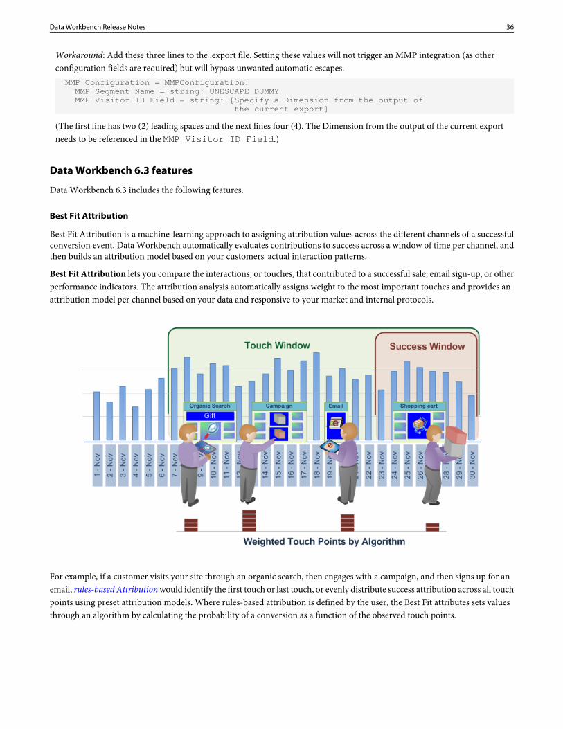
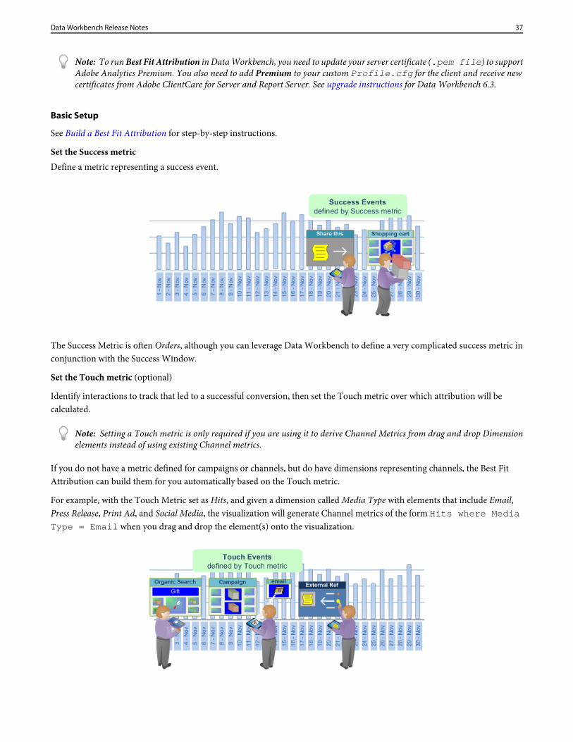
Set the Touch metric (optional)
Identify interactions to track that led to a successful conversion, then set the Touch metric over which attribution will becalculated.
Note: Setting a Touch metric is only required if you are using it to derive Channel Metrics from drag and drop Dimensionelements instead of using existing Channel metrics.
If you do not have a metric defined for campaigns or channels, but do have dimensions representing channels, the Best FitAttribution can build them for you automatically based on the Touch metric.
For example, with the Touch Metric set as Hits, and given a dimension called Media Type with elements that include Email,Press Release, Print Ad, and Social Media, the visualization will generate Channel metrics of the form Hits where MediaType = Email when you drag and drop the element(s) onto the visualization.
37Data Workbench Release Notes
The Touch metric then determines the allocation of attribution scores to identify marketing interactions considered influentialfor success, allowing you to qualify marketing touches for the population identified in the Success window. You can set metricsuch as Page Views or Hits, or use customized touch metrics specific to your needs.
In many cases, the Touch window should include the Success window to evaluate a long lead time in the sales cycle.
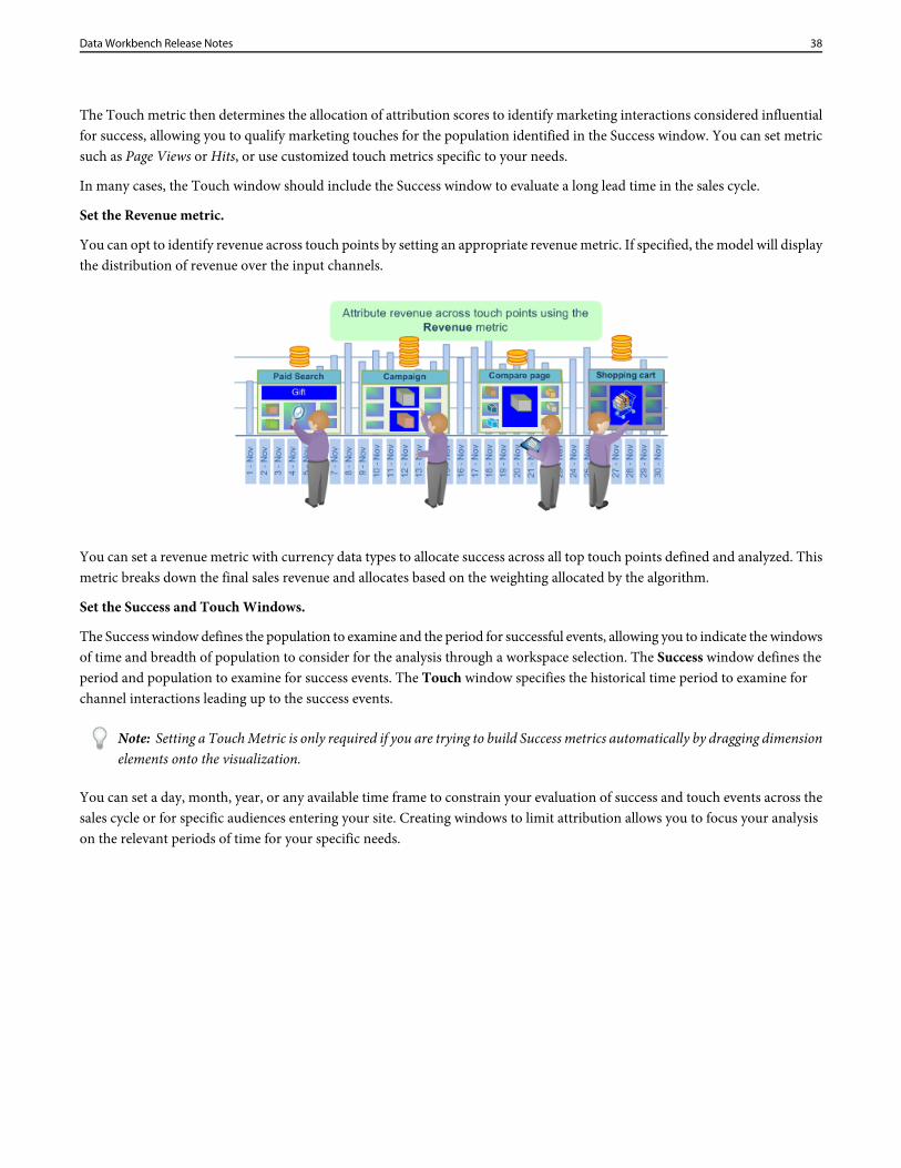
Set the Revenue metric.
You can opt to identify revenue across touch points by setting an appropriate revenue metric. If specified, the model will displaythe distribution of revenue over the input channels.
You can set a revenue metric with currency data types to allocate success across all top touch points defined and analyzed. Thismetric breaks down the final sales revenue and allocates based on the weighting allocated by the algorithm.
Set the Success and Touch Windows.
The Success window defines the population to examine and the period for successful events, allowing you to indicate the windowsof time and breadth of population to consider for the analysis through a workspace selection. The Success window defines theperiod and population to examine for success events. The Touch window specifies the historical time period to examine forchannel interactions leading up to the success events.
Note: Setting a Touch Metric is only required if you are trying to build Success metrics automatically by dragging dimensionelements onto the visualization.
You can set a day, month, year, or any available time frame to constrain your evaluation of success and touch events across thesales cycle or for specific audiences entering your site. Creating windows to limit attribution allows you to focus your analysison the relevant periods of time for your specific needs.
38Data Workbench Release Notes
In many cases, you will want the Touch window to include the Success window to let you extend your analysis over a long leadtime based on your sales window. Or you can track and analyze touches separate from the success event.
Select the Channels.
When entering channels you have two choices.
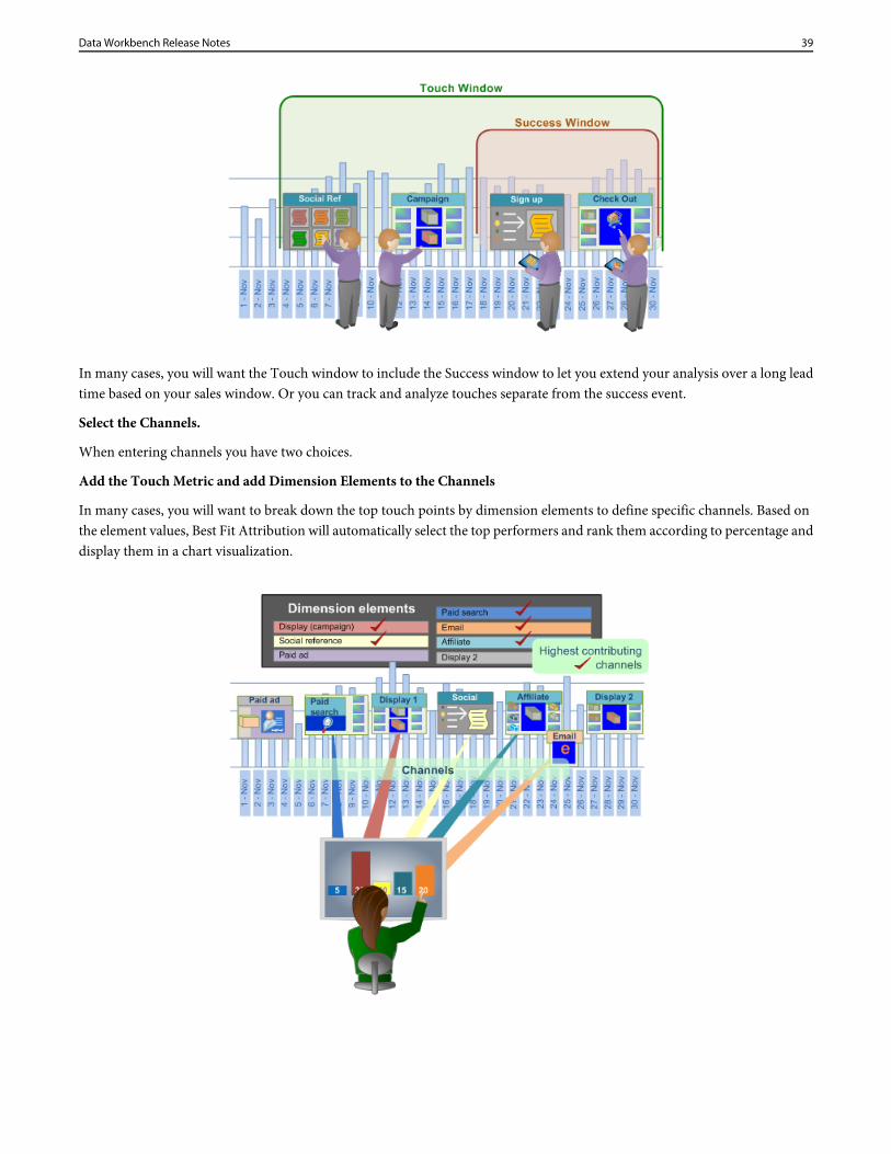
Add the Touch Metric and add Dimension Elements to the Channels
In many cases, you will want to break down the top touch points by dimension elements to define specific channels. Based onthe element values, Best Fit Attribution will automatically select the top performers and rank them according to percentage anddisplay them in a chart visualization.
39Data Workbench Release Notes
An attribution model will be built by drawing on the visitors who interacted during your Success window and examining thechannel Touches during the Touch window that did or did not result in a successful event.
Breaking Down by Channels
When entering channels you have two options:
• Add a Touch Metric and then add Dimension Elements for the Channels.
or
• Create metrics that filter for the channel elements that you want to evaluate.
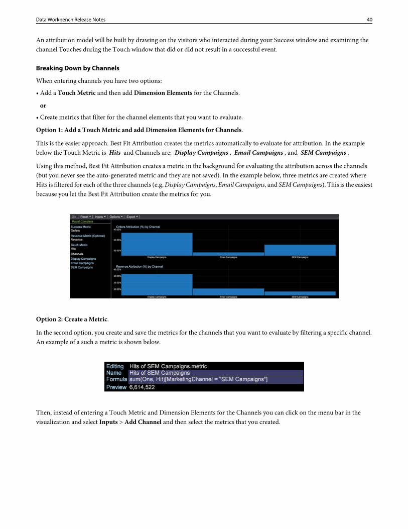
Option 1: Add a Touch Metric and add Dimension Elements for Channels.
This is the easier approach. Best Fit Attribution creates the metrics automatically to evaluate for attribution. In the examplebelow the Touch Metric is Hits and Channels are: Display Campaigns , Email Campaigns , and SEM Campaigns .
Using this method, Best Fit Attribution creates a metric in the background for evaluating the attribution across the channels(but you never see the auto-generated metric and they are not saved). In the example below, three metrics are created whereHits is filtered for each of the three channels (e.g, Display Campaigns, Email Campaigns, and SEM Campaigns). This is the easiestbecause you let the Best Fit Attribution create the metrics for you.
Option 2: Create a Metric.
In the second option, you create and save the metrics for the channels that you want to evaluate by filtering a specific channel.An example of a such a metric is shown below.
Then, instead of entering a Touch Metric and Dimension Elements for the Channels you can click on the menu bar in thevisualization and select Inputs > Add Channel and then select the metrics that you created.
40Data Workbench Release Notes
See the example of the second method below. You can see that the results of both options are identical.Build a Best Fit Attribution Model
Open Best Fit Attribution from the Premium menu and follow these steps to build a Best Fit Attribution model.
See an overview of Best Fit Attribution.
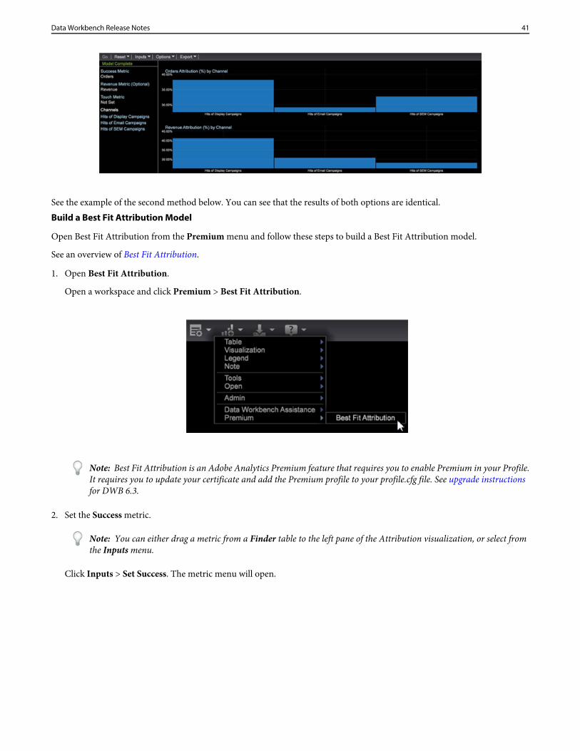
1. Open Best Fit Attribution.
Open a workspace and click Premium > Best Fit Attribution.
Note: Best Fit Attribution is an Adobe Analytics Premium feature that requires you to enable Premium in your Profile.It requires you to update your certificate and add the Premium profile to your profile.cfg file. See upgrade instructionsfor DWB 6.3.
2. Set the Success metric.
Note: You can either drag a metric from a Finder table to the left pane of the Attribution visualization, or select fromthe Inputs menu.
Click Inputs > Set Success. The metric menu will open.
41Data Workbench Release Notes
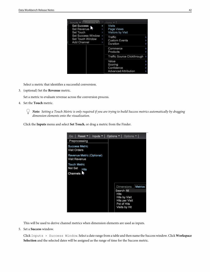
Select a metric that identifies a successful conversion.
3. (optional) Set the Revenue metric.
Set a metric to evaluate revenue across the conversion process.
4. Set the Touch metric.
Note: Setting a Touch Metric is only required if you are trying to build Success metrics automatically by draggingdimension elements onto the visualization.
Click the Inputs menu and select Set Touch, or drag a metric from the Finder.
This will be used to derive channel metrics when dimension elements are used as inputs.
5. Set a Success window.
Click Inputs > Success Window. Select a date range from a table and then name the Success window. Click WorkspaceSelection and the selected dates will be assigned as the range of time for the Success metric.
42Data Workbench Release Notes
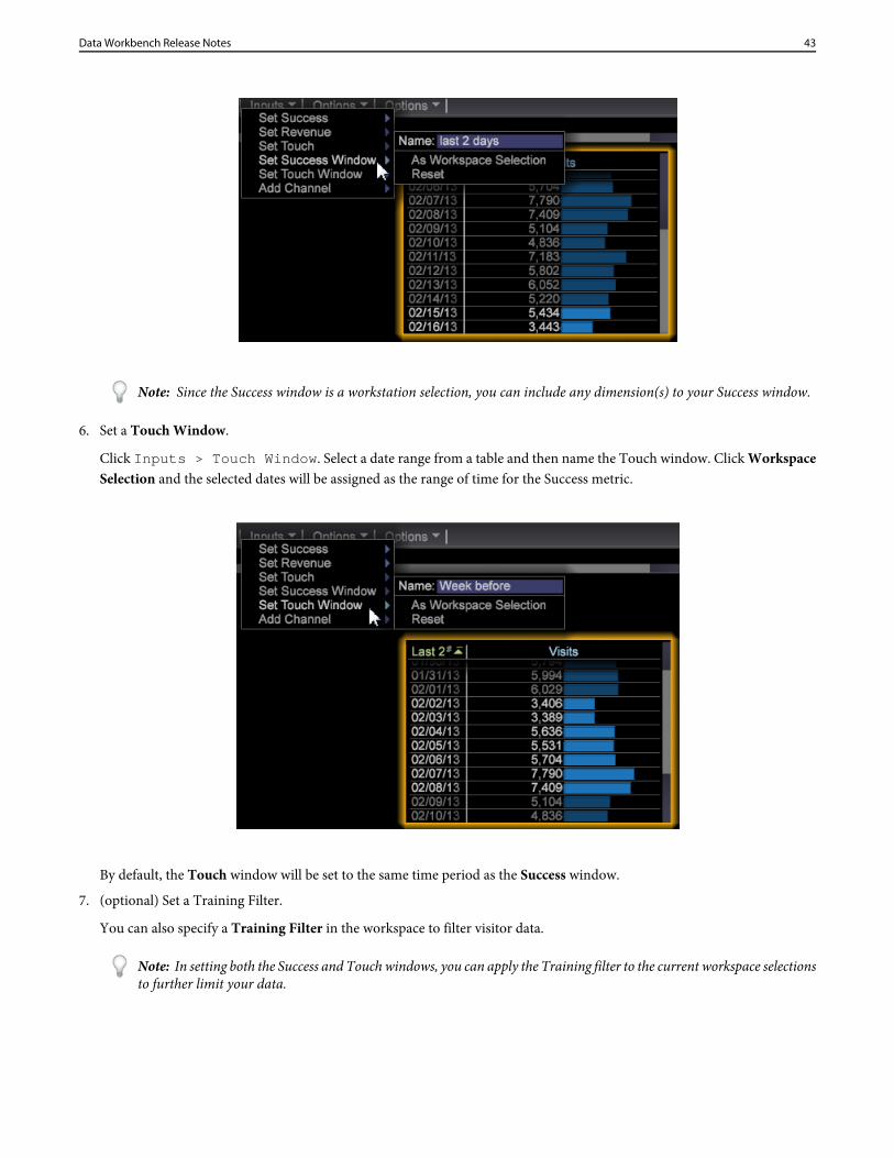
Note: Since the Success window is a workstation selection, you can include any dimension(s) to your Success window.
6. Set a Touch Window.
Click Inputs > Touch Window. Select a date range from a table and then name the Touch window. Click WorkspaceSelection and the selected dates will be assigned as the range of time for the Success metric.
By default, the Touch window will be set to the same time period as the Success window.
7. (optional) Set a Training Filter.
You can also specify a Training Filter in the workspace to filter visitor data.
Note: In setting both the Success and Touch windows, you can apply the Training filter to the current workspace selectionsto further limit your data.
43Data Workbench Release Notes
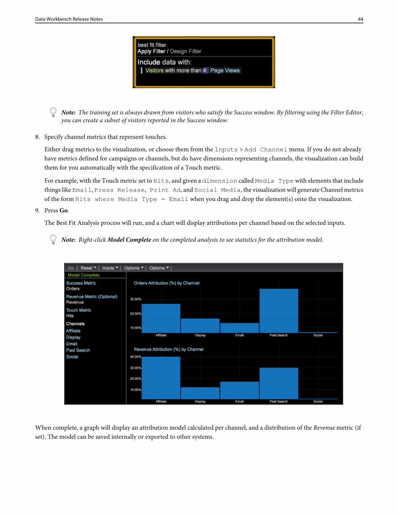
Note: The training set is always drawn from visitors who satisfy the Success window. By filtering using the Filter Editor,you can create a subset of visitors reported in the Success window.
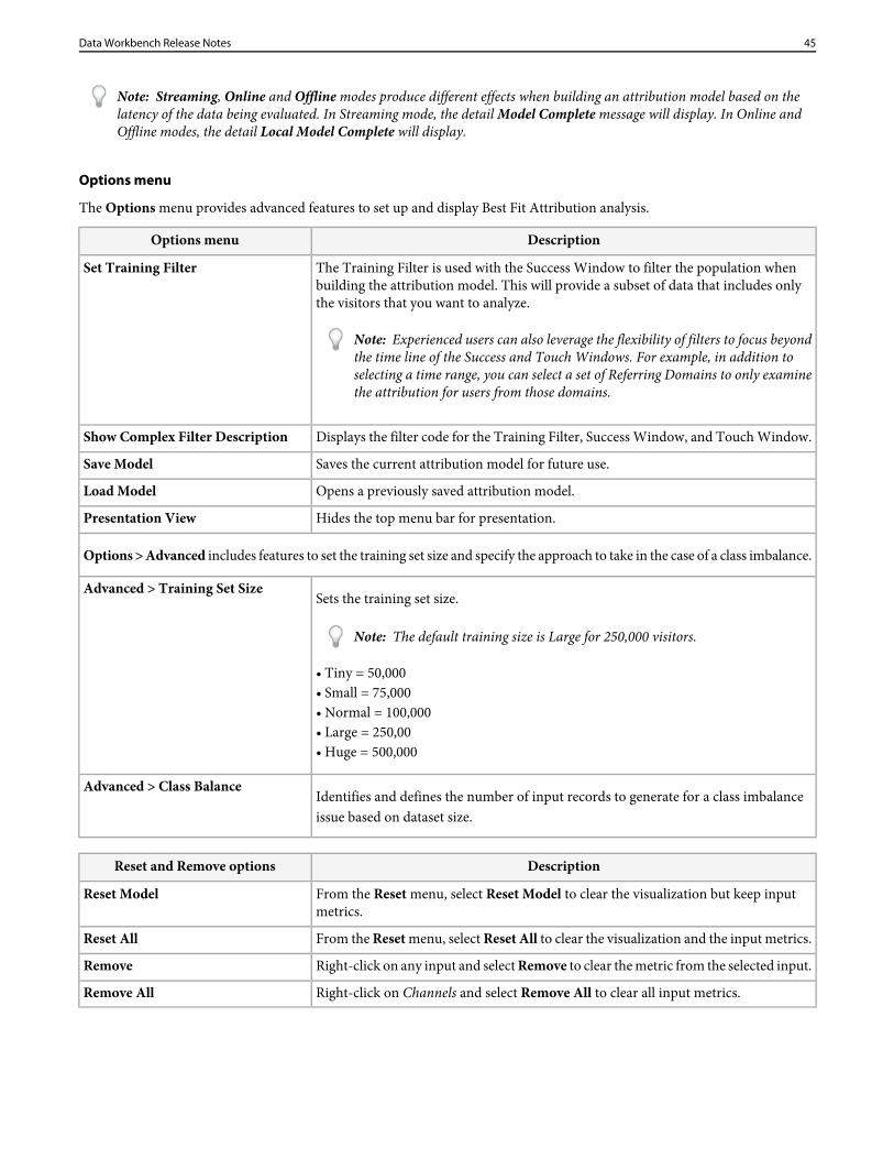
8. Specify channel metrics that represent touches.
Either drag metrics to the visualization, or choose them from the Inputs > Add Channel menu. If you do not alreadyhave metrics defined for campaigns or channels, but do have dimensions representing channels, the visualization can buildthem for you automatically with the specification of a Touch metric.
For example, with the Touch metric set to Hits, and given a dimension called Media Type with elements that includethings like Email, Press Release, Print Ad, and Social Media, the visualization will generate Channel metricsof the form Hits where Media Type = Email when you drag and drop the element(s) onto the visualization.
9. Press Go.
The Best Fit Analysis process will run, and a chart will display attributions per channel based on the selected inputs.
Note: Right-click Model Complete on the completed analysis to see statistics for the attribution model.
When complete, a graph will display an attribution model calculated per channel, and a distribution of the Revenue metric (ifset). The model can be saved internally or exported to other systems.
44Data Workbench Release Notes
Note: Streaming, Online and Offline modes produce different effects when building an attribution model based on thelatency of the data being evaluated. In Streaming mode, the detail Model Complete message will display. In Online andOffline modes, the detail Local Model Complete will display.
Options menu
The Options menu provides advanced features to set up and display Best Fit Attribution analysis.
DescriptionOptions menu
The Training Filter is used with the Success Window to filter the population whenbuilding the attribution model. This will provide a subset of data that includes onlythe visitors that you want to analyze.
Set Training Filter
Note: Experienced users can also leverage the flexibility of filters to focus beyondthe time line of the Success and Touch Windows. For example, in addition toselecting a time range, you can select a set of Referring Domains to only examinethe attribution for users from those domains.
Displays the filter code for the Training Filter, Success Window, and Touch Window.Show Complex Filter Description
Saves the current attribution model for future use.Save Model
Opens a previously saved attribution model.Load Model
Hides the top menu bar for presentation.Presentation View
Options > Advanced includes features to set the training set size and specify the approach to take in the case of a class imbalance.
Sets the training set size.Advanced > Training Set Size
Note: The default training size is Large for 250,000 visitors.
• Tiny = 50,000• Small = 75,000• Normal = 100,000• Large = 250,00• Huge = 500,000
Identifies and defines the number of input records to generate for a class imbalanceissue based on dataset size.
Advanced > Class Balance
DescriptionReset and Remove options
From the Reset menu, select Reset Model to clear the visualization but keep inputmetrics.
Reset Model
From the Reset menu, select Reset All to clear the visualization and the input metrics.Reset All
Right-click on any input and select Remove to clear the metric from the selected input.Remove
Right-click on Channels and select Remove All to clear all input metrics.Remove All
45Data Workbench Release Notes
Chord Visualization
The Chord visualization allows you to show both the proportion and correlation between metrics, displaying larger chords asan indication of a stronger correlation.
The Chord visualization lets you see identify correlations between metrics, allowing you to add and easily evaluate possiblecorrelations. It also provides another view into any previously built Correlation Matrix. Using the Chord visualization, youcannot identify a positive or negative correlation between the metrics—only that a correlation exists. In certain cases, determininga direct or inverse relationship can be identified by applying counter metrics.
1. Open the Chord visualization.
In the workspace, right-click Visualization > Predictive Analytics > Chord.
2. Select a Dimension from the menu.
A blank visualization will open allowing you to select a dimension. The dimension name will appear at the top of the blankchord visualization.
Note: If you already have a Correlation Matrix open in the workspace, you can also render it as a Chord visualization.
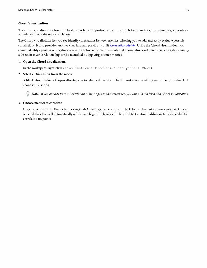
3. Choose metrics to correlate.
Drag metrics from the Finder by clicking Ctrl-Alt to drag metrics from the table to the chart. After two or more metrics areselected, the chart will automatically refresh and begin displaying correlation data. Continue adding metrics as needed tocorrelate data points.
46Data Workbench Release Notes
The Chord visualization displays the proportion of the whole represented by the area of each segment. Continue to addmetrics as need to identify and investigate significant relationships.
47Data Workbench Release Notes
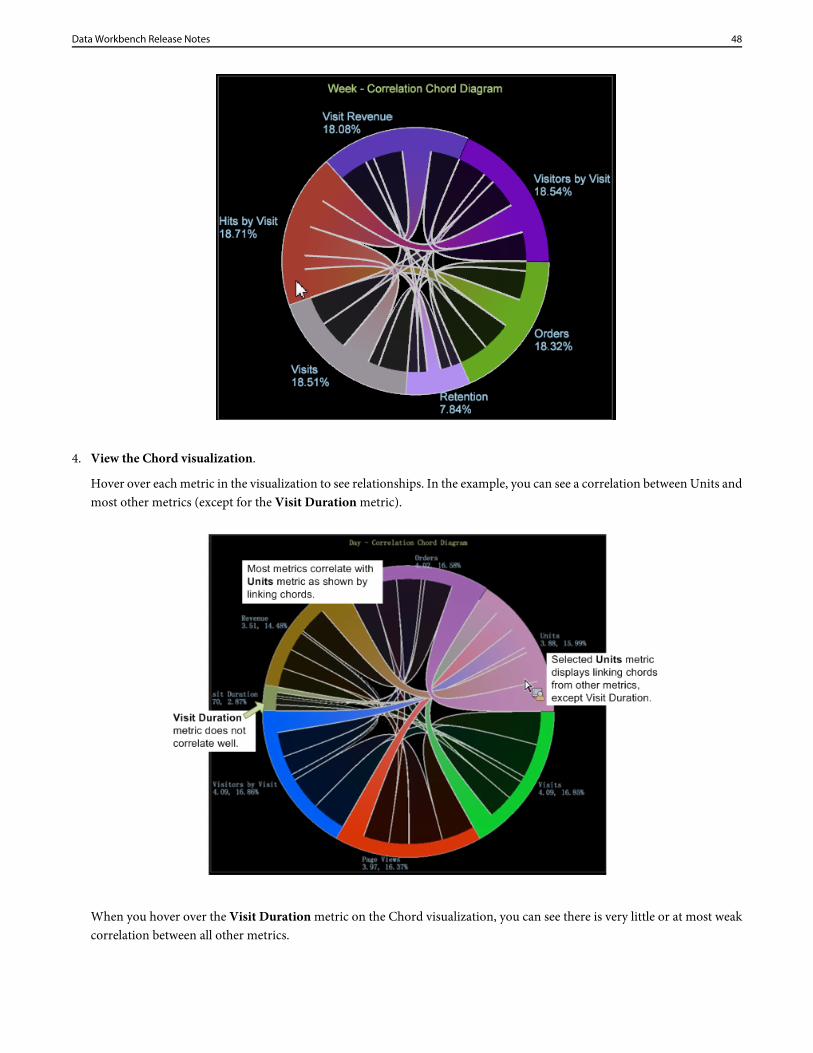
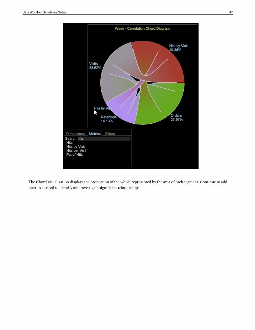
4. View the Chord visualization.
Hover over each metric in the visualization to see relationships. In the example, you can see a correlation between Units andmost other metrics (except for the Visit Duration metric).
When you hover over the Visit Duration metric on the Chord visualization, you can see there is very little or at most weakcorrelation between all other metrics.
48Data Workbench Release Notes
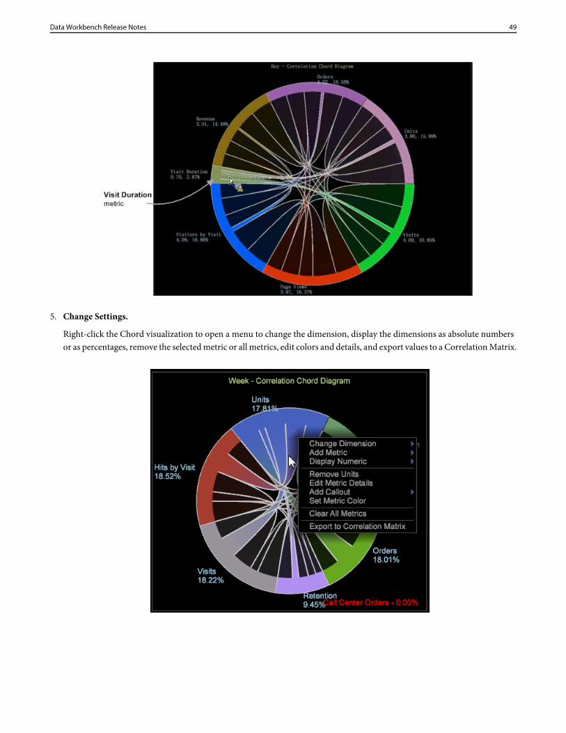
5. Change Settings.
Right-click the Chord visualization to open a menu to change the dimension, display the dimensions as absolute numbersor as percentages, remove the selected metric or all metrics, edit colors and details, and export values to a Correlation Matrix.
49Data Workbench Release Notes
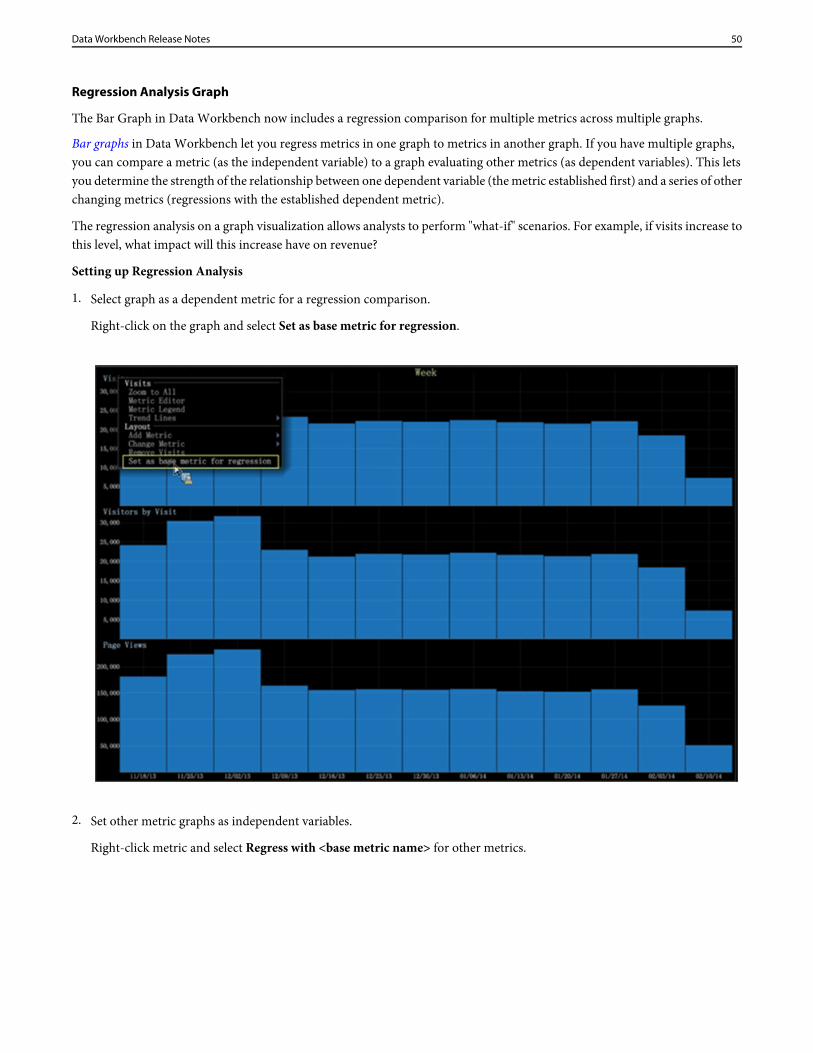
Regression Analysis Graph
The Bar Graph in Data Workbench now includes a regression comparison for multiple metrics across multiple graphs.
Bar graphs in Data Workbench let you regress metrics in one graph to metrics in another graph. If you have multiple graphs,you can compare a metric (as the independent variable) to a graph evaluating other metrics (as dependent variables). This letsyou determine the strength of the relationship between one dependent variable (the metric established first) and a series of otherchanging metrics (regressions with the established dependent metric).
The regression analysis on a graph visualization allows analysts to perform "what-if" scenarios. For example, if visits increase tothis level, what impact will this increase have on revenue?
Setting up Regression Analysis
1. Select graph as a dependent metric for a regression comparison.
Right-click on the graph and select Set as base metric for regression.
2. Set other metric graphs as independent variables.
Right-click metric and select Regress with <base metric name> for other metrics.
50Data Workbench Release Notes
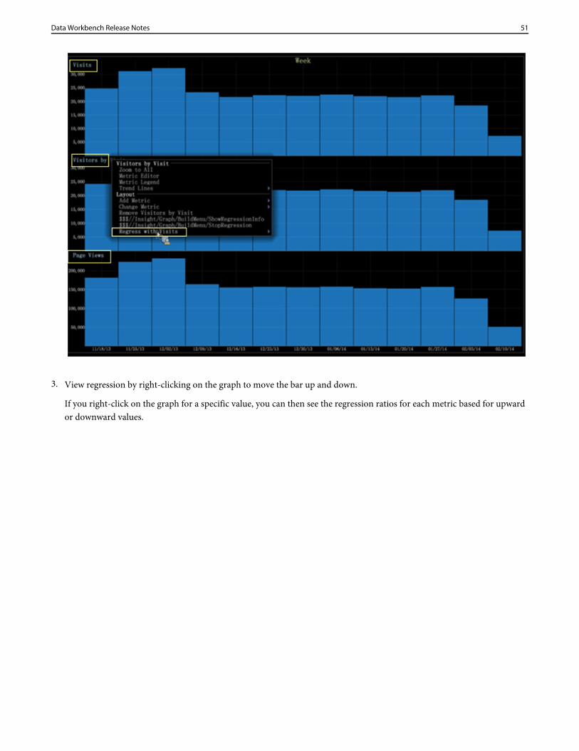
3. View regression by right-clicking on the graph to move the bar up and down.
If you right-click on the graph for a specific value, you can then see the regression ratios for each metric based for upwardor downward values.
51Data Workbench Release Notes
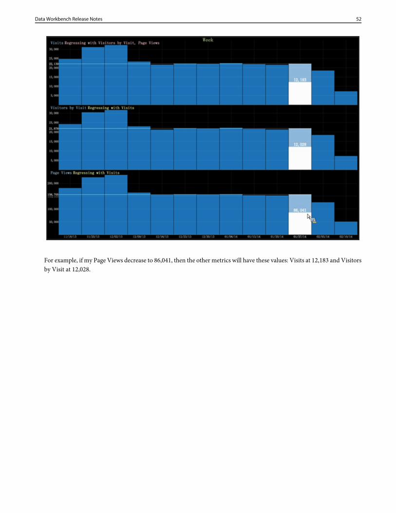
For example, if my Page Views decrease to 86,041, then the other metrics will have these values: Visits at 12,183 and Visitorsby Visit at 12,028.
52Data Workbench Release Notes
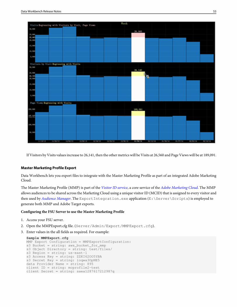
If Visitors by Visits values increase to 26,141, then the other metrics will be Visits at 26,560 and Page Views will be at 189,091.
Master Marketing Profile Export
Data Workbench lets you export files to integrate with the Master Marketing Profile as part of an integrated Adobe MarketingCloud.
The Master Marketing Profile (MMP) is part of the Visitor ID service, a core service of the Adobe Marketing Cloud. The MMPallows audiences to be shared across the Marketing Cloud using a unique visitor ID (MCID) that is assigned to every visitor andthen used by Audience Manager. The ExportIntegration.exe application (E:\Server\Scripts) is employed togenerate both MMP and Adobe Target exports.
Configuring the FSU Server to use the Master Marketing Profile
1. Access your FSU server.2. Open the MMPExport.cfg file. (Server/Admin/Export/MMPExport.cfg).3. Enter values in the all fields as required. For example:
Sample MMPExport.cfgMMP Export Configuration = MMPExportConfiguration:s3 Bucket = string: aws_bucket_for_mmps3 Object Directory = string: test/files/s3 Region = string: us-east-1s3 Access Key = string: ZZKI62OO5YBAs3 Secret Key = string: ioqwa3OpNE5data Provider Name = string: 895client ID = string: mcprofile2-testclient Secret = string: saea1287617212987q
53Data Workbench Release Notes
username = string: mmptestpassword = string: pass
Definition of parameters. (The s3 information required for MMP (s3) can be obtained from Audience Manager team.)
Note: MMP/AAM integration relies on Amazon's s3 bucket for data transfer.
DefinitionParameter
The AWS S3 bucket where the export is transferred to.s3 Bucket
A path to save s3 files. This supports sub-directories.s3 Object Directory
Important: Space and multibyte characters are not allowed in the path and will createerrors in the export. (The hypen is allowed).
The AWS s3 Region where the export is sent to. Ex. us-east-1s3 Region
AWS s3 Access Keys3 Access Key
AWS s3 Secret Keys3 Secret Key
This will be the folder name that is used for storing segments and traits in AAM respectively.This should be unique per customer.
data Provider Name
This is a unique client ID provided to a customer when he/she is provisioned for MMP.client ID
This is a unique client secret provided to a customer when he/she is provisioned for MMP.client Secret
MMP usernameusername
MMP passwordpassword
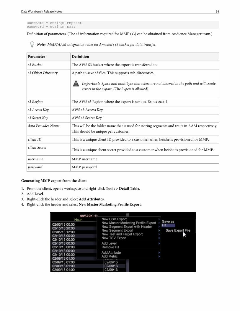
Generating MMP export from the client
1. From the client, open a workspace and right-click Tools > Detail Table.2. Add Level.3. Right-click the header and select Add Attributes.4. Right-click the header and select New Master Marketing Profile Export.
54Data Workbench Release Notes
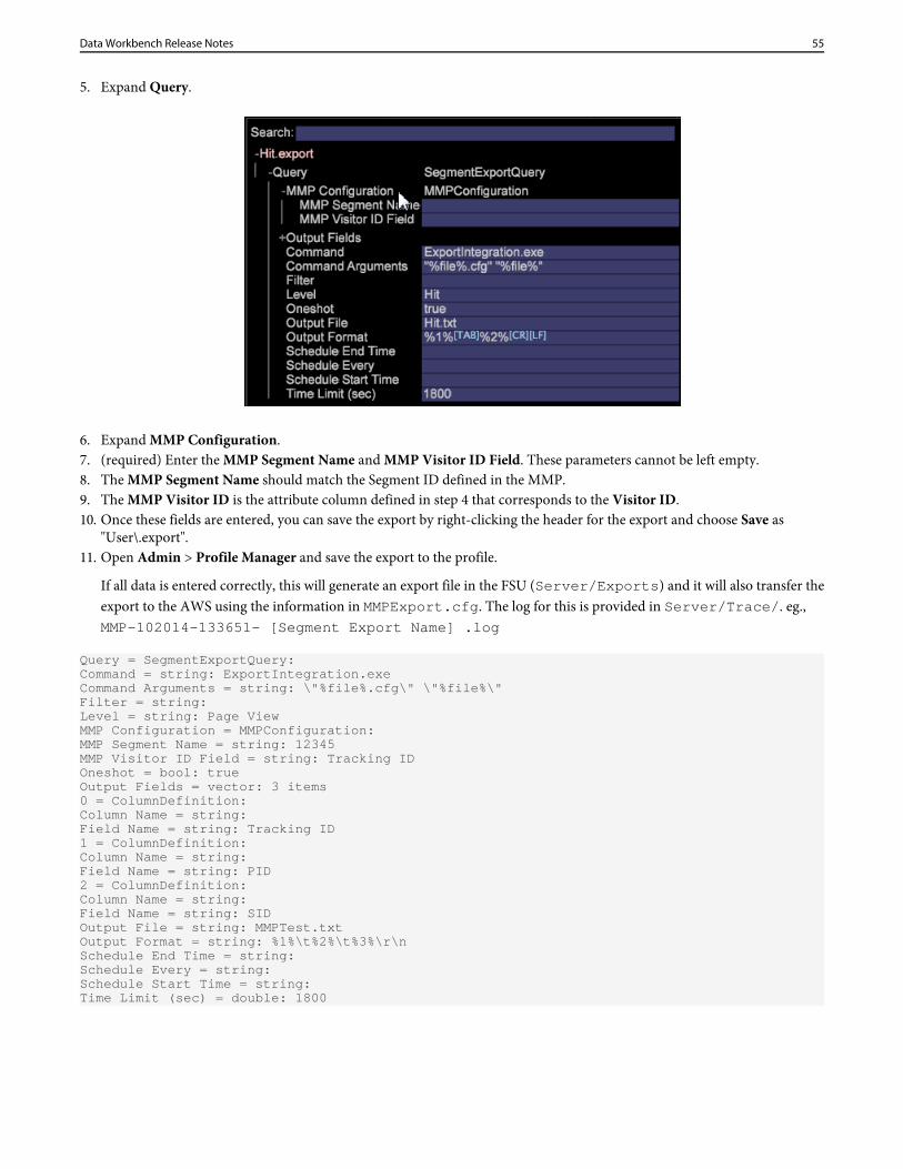
5. Expand Query.
6. Expand MMP Configuration.7. (required) Enter the MMP Segment Name and MMP Visitor ID Field. These parameters cannot be left empty.8. The MMP Segment Name should match the Segment ID defined in the MMP.9. The MMP Visitor ID is the attribute column defined in step 4 that corresponds to the Visitor ID.10. Once these fields are entered, you can save the export by right-clicking the header for the export and choose Save as
"User\.export".11. Open Admin > Profile Manager and save the export to the profile.
If all data is entered correctly, this will generate an export file in the FSU (Server/Exports) and it will also transfer theexport to the AWS using the information in MMPExport.cfg. The log for this is provided in Server/Trace/. eg.,MMP-102014-133651- [Segment Export Name] .log
Query = SegmentExportQuery:Command = string: ExportIntegration.exeCommand Arguments = string: \"%file%.cfg\" \"%file%\"Filter = string:Level = string: Page ViewMMP Configuration = MMPConfiguration:MMP Segment Name = string: 12345MMP Visitor ID Field = string: Tracking IDOneshot = bool: trueOutput Fields = vector: 3 items0 = ColumnDefinition:Column Name = string:Field Name = string: Tracking ID1 = ColumnDefinition:Column Name = string:Field Name = string: PID2 = ColumnDefinition:Column Name = string:Field Name = string: SIDOutput File = string: MMPTest.txtOutput Format = string: %1%\t%2%\t%3%\r\nSchedule End Time = string:Schedule Every = string:Schedule Start Time = string:Time Limit (sec) = double: 1800
55Data Workbench Release Notes
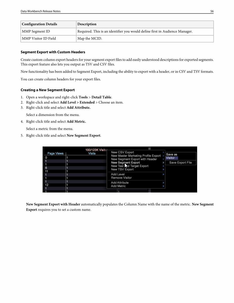
DescriptionConfiguration Details
Required. This is an identifier you would define first in Audience Manager.MMP Segment ID
Map the MCID.MMP Visitor ID Field
Segment Export with Custom Headers
Create custom column export headers for your segment export files to add easily understood descriptions for exported segments.This export feature also lets you output as TSV and CSV files.
New functionality has been added to Segment Export, including the ability to export with a header, or in CSV and TSV formats.
You can create column headers for your export files.
Creating a New Segment Export
1. Open a workspace and right-click Tools > Detail Table.2. Right-click and select Add Level > Extended > Choose an item.3. Right-click title and select Add Attribute.
Select a dimension from the menu.
4. Right-click title and select Add Metric.
Select a metric from the menu.
5. Right-click title and select New Segment Export.
New Segment Export with Header automatically populates the Column Name with the name of the metric. New SegmentExport requires you to set a custom name.
56Data Workbench Release Notes
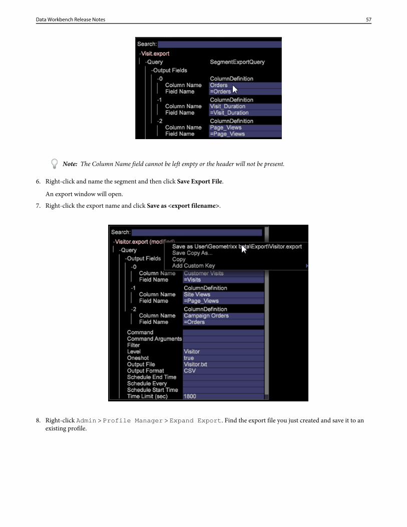
Note: The Column Name field cannot be left empty or the header will not be present.
6. Right-click and name the segment and then click Save Export File.
An export window will open.
7. Right-click the export name and click Save as <export filename>.
8. Right-click Admin > Profile Manager > Expand Export. Find the export file you just created and save it to anexisting profile.
57Data Workbench Release Notes
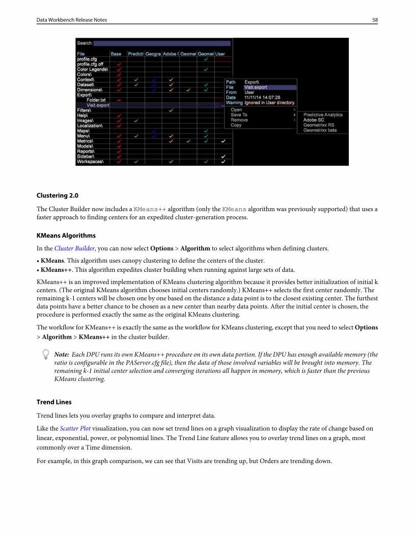
Clustering 2.0
The Cluster Builder now includes a KMeans++ algorithm (only the KMeans algorithm was previously supported) that uses afaster approach to finding centers for an expedited cluster-generation process.
KMeans Algorithms
In the Cluster Builder, you can now select Options > Algorithm to select algorithms when defining clusters.
• KMeans. This algorithm uses canopy clustering to define the centers of the cluster.• KMeans++. This algorithm expedites cluster building when running against large sets of data.
KMeans++ is an improved implementation of KMeans clustering algorithm because it provides better initialization of initial kcenters. (The original KMeans algorithm chooses initial centers randomly.) KMeans++ selects the first center randomly. Theremaining k-1 centers will be chosen one by one based on the distance a data point is to the closest existing center. The furthestdata points have a better chance to be chosen as a new center than nearby data points. After the initial center is chosen, theprocedure is performed exactly the same as the original KMeans clustering.
The workflow for KMeans++ is exactly the same as the workflow for KMeans clustering, except that you need to select Options> Algorithm > KMeans++ in the cluster builder.
Note: Each DPU runs its own KMeans++ procedure on its own data portion. If the DPU has enough available memory (theratio is configurable in the PAServer.cfg file), then the data of those involved variables will be brought into memory. Theremaining k-1 initial center selection and converging iterations all happen in memory, which is faster than the previousKMeans clustering.
Trend Lines
Trend lines lets you overlay graphs to compare and interpret data.
Like the Scatter Plot visualization, you can now set trend lines on a graph visualization to display the rate of change based onlinear, exponential, power, or polynomial lines. The Trend Line feature allows you to overlay trend lines on a graph, mostcommonly over a Time dimension.
For example, in this graph comparison, we can see that Visits are trending up, but Orders are trending down.
58Data Workbench Release Notes
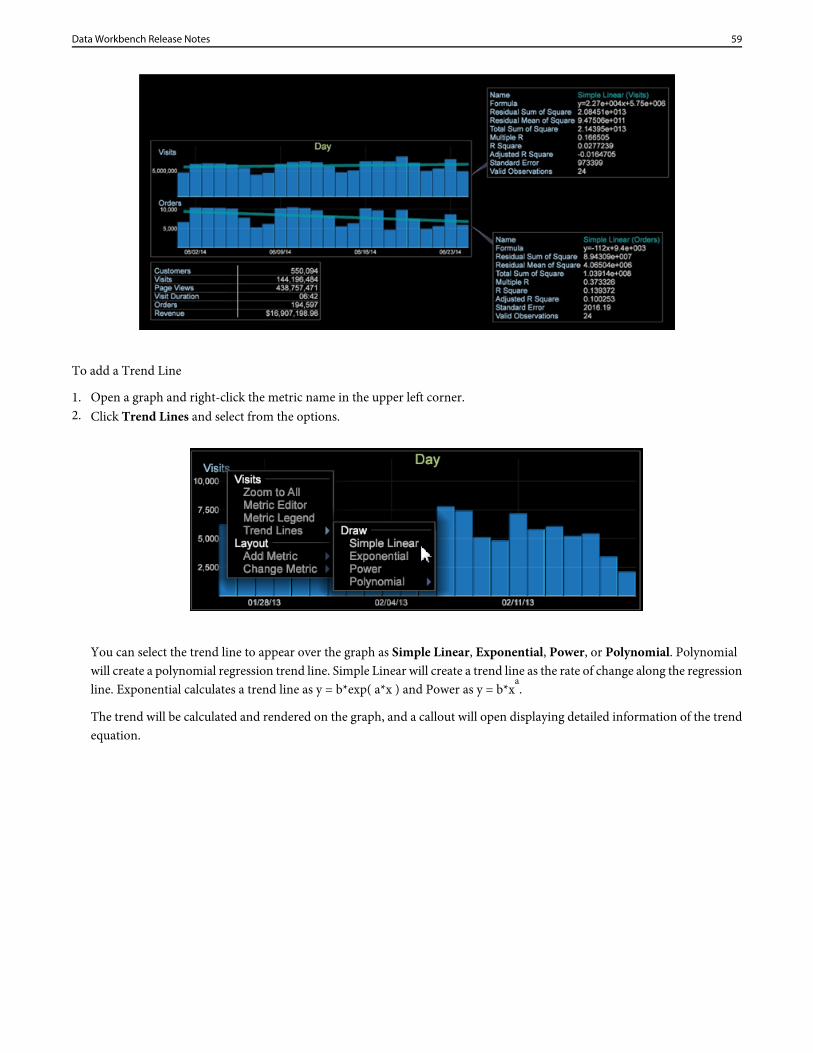
To add a Trend Line
1. Open a graph and right-click the metric name in the upper left corner.2. Click Trend Lines and select from the options.
You can select the trend line to appear over the graph as Simple Linear, Exponential, Power, or Polynomial. Polynomialwill create a polynomial regression trend line. Simple Linear will create a trend line as the rate of change along the regressionline. Exponential calculates a trend line as y = b*exp( a*x ) and Power as y = b*x
a.
The trend will be calculated and rendered on the graph, and a callout will open displaying detailed information of the trendequation.
59Data Workbench Release Notes
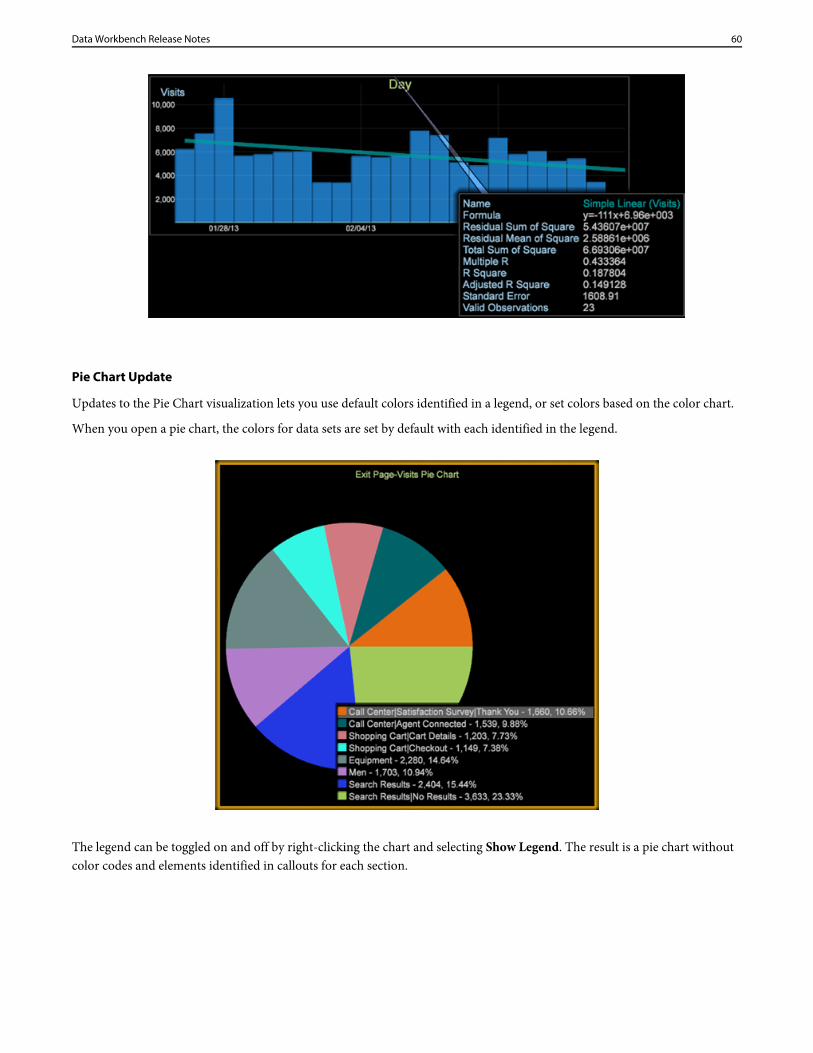
Pie Chart Update
Updates to the Pie Chart visualization lets you use default colors identified in a legend, or set colors based on the color chart.
When you open a pie chart, the colors for data sets are set by default with each identified in the legend.
The legend can be toggled on and off by right-clicking the chart and selecting Show Legend. The result is a pie chart withoutcolor codes and elements identified in callouts for each section.
60Data Workbench Release Notes
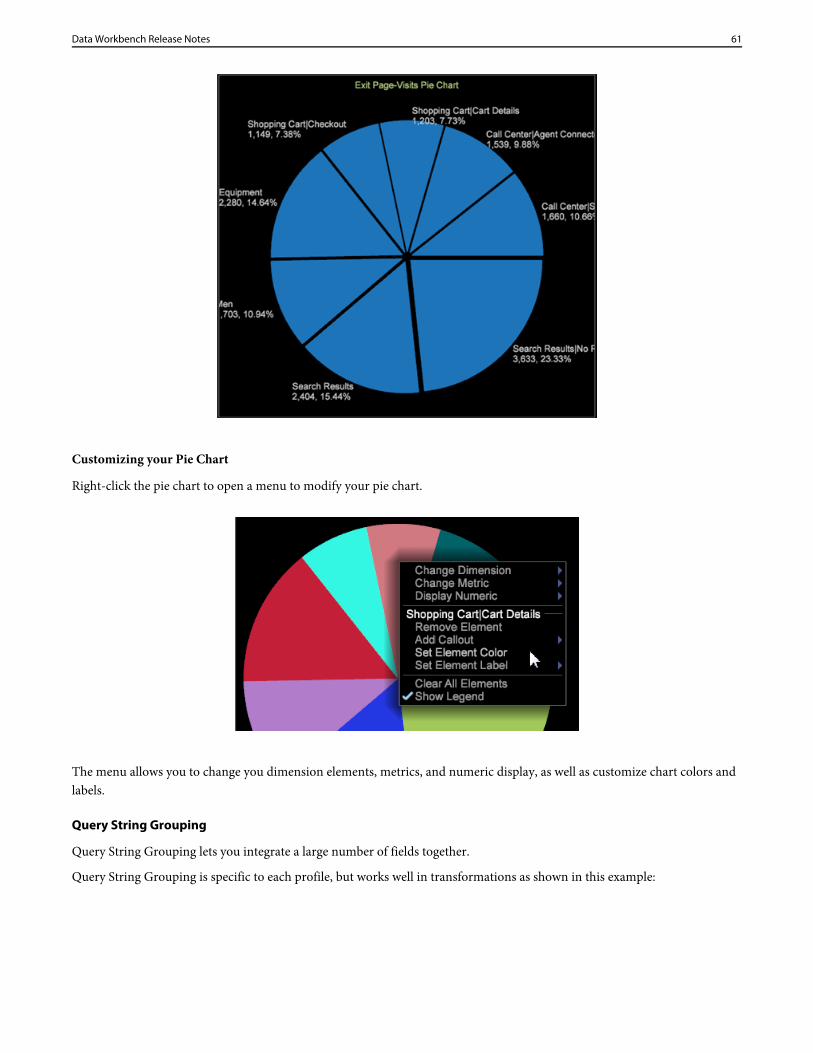
Customizing your Pie Chart
Right-click the pie chart to open a menu to modify your pie chart.
The menu allows you to change you dimension elements, metrics, and numeric display, as well as customize chart colors andlabels.
Query String Grouping
Query String Grouping lets you integrate a large number of fields together.
Query String Grouping is specific to each profile, but works well in transformations as shown in this example:
61Data Workbench Release Notes
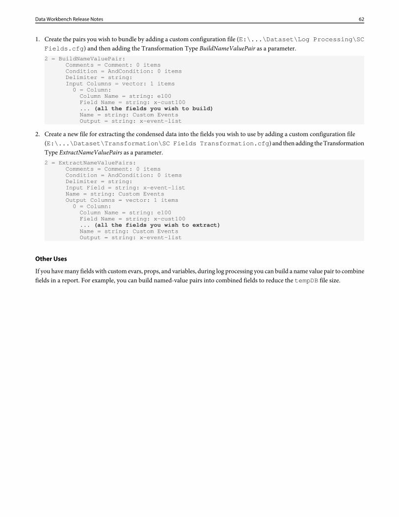
1. Create the pairs you wish to bundle by adding a custom configuration file (E:\...\Dataset\Log Processing\SCFields.cfg) and then adding the Transformation Type BuildNameValuePair as a parameter.2 = BuildNameValuePair: Comments = Comment: 0 items Condition = AndCondition: 0 items Delimiter = string: Input Columns = vector: 1 items 0 = Column: Column Name = string: e100 Field Name = string: x-cust100 ... (all the fields you wish to build) Name = string: Custom Events Output = string: x-event-list
2. Create a new file for extracting the condensed data into the fields you wish to use by adding a custom configuration file(E:\...\Dataset\Transformation\SC Fields Transformation.cfg) and then adding the TransformationType ExtractNameValuePairs as a parameter.2 = ExtractNameValuePairs: Comments = Comment: 0 items Condition = AndCondition: 0 items Delimiter = string: Input Field = string: x-event-list Name = string: Custom Events Output Columns = vector: 1 items 0 = Column: Column Name = string: e100 Field Name = string: x-cust100 ... (all the fields you wish to extract) Name = string: Custom Events Output = string: x-event-list
Other Uses
If you have many fields with custom evars, props, and variables, during log processing you can build a name value pair to combinefields in a report. For example, you can build named-value pairs into combined fields to reduce the tempDB file size.
62Data Workbench Release Notes
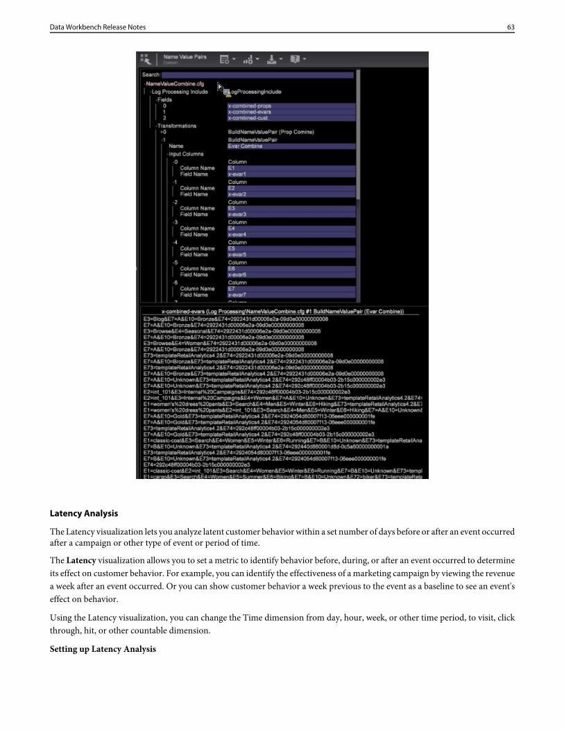
Latency Analysis
The Latency visualization lets you analyze latent customer behavior within a set number of days before or after an event occurredafter a campaign or other type of event or period of time.
The Latency visualization allows you to set a metric to identify behavior before, during, or after an event occurred to determineits effect on customer behavior. For example, you can identify the effectiveness of a marketing campaign by viewing the revenuea week after an event occurred. Or you can show customer behavior a week previous to the event as a baseline to see an event'seffect on behavior.
Using the Latency visualization, you can change the Time dimension from day, hour, week, or other time period, to visit, clickthrough, hit, or other countable dimension.
Setting up Latency Analysis
63Data Workbench Release Notes
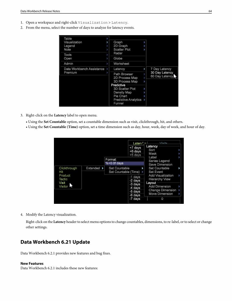
1. Open a workspace and right-click Visualization > Latency.2. From the menu, select the number of days to analyze for latency events.
3. Right-click on the Latency label to open menu.
• Using the Set Countable option, set a countable dimension such as visit, clickthrough, hit, and others.• Using the Set Countable (Time) option, set a time dimension such as day, hour, week, day of week, and hour of day.
4. Modify the Latency visualization.
Right-click on the Latency header to select menu options to change countables, dimensions, to re-label, or to select or changeother settings.
Data Workbench 6.21 Update
Data Workbench 6.2.1 provides new features and bug fixes.
New FeaturesData Workbench 6.2.1 includes these new features:
64Data Workbench Release Notes
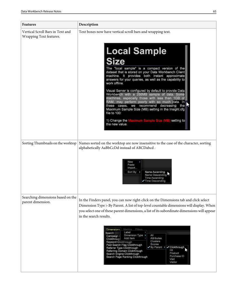
DescriptionFeatures
Text boxes now have vertical scroll bars and wrapping text.Vertical Scroll Bars in Text andWrapping Text features.
Names sorted on the worktop are now insensitive to the case of the character, sortingalphabetically AaBbCcDd instead of ABCDabcd .
Sorting Thumbnails on the worktop
In the Finders panel, you can now right-click on the Dimensions tab and click selectDimension Type > By Parent. A list of top-level countable dimensions will display. When
Searching dimensions based on theparent dimension.
you select one of these parent dimensions, a list of its subordinate dimensions will appearin the search results.
65Data Workbench Release Notes
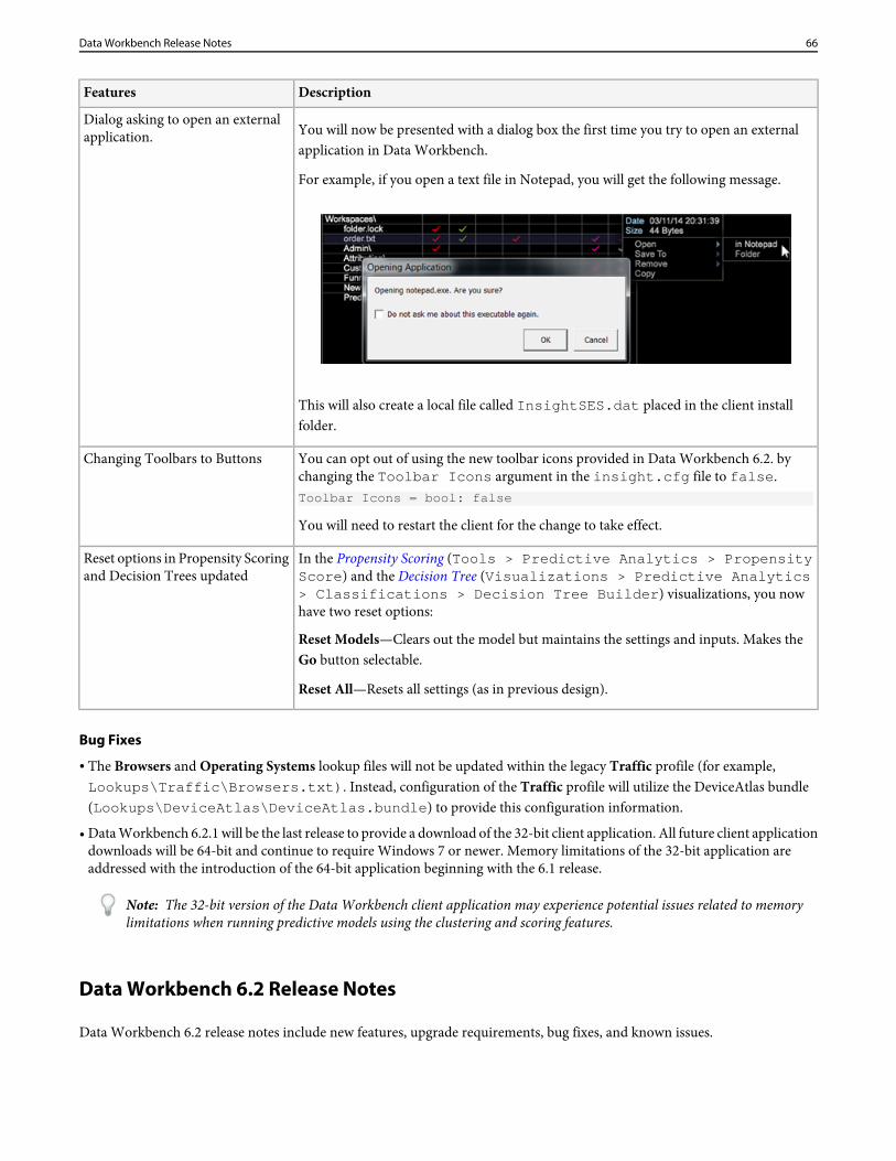
DescriptionFeatures
You will now be presented with a dialog box the first time you try to open an externalapplication in Data Workbench.
Dialog asking to open an externalapplication.
For example, if you open a text file in Notepad, you will get the following message.
This will also create a local file called InsightSES.dat placed in the client installfolder.
You can opt out of using the new toolbar icons provided in Data Workbench 6.2. bychanging the Toolbar Icons argument in the insight.cfg file to false.Toolbar Icons = bool: false
Changing Toolbars to Buttons
You will need to restart the client for the change to take effect.
In the Propensity Scoring (Tools > Predictive Analytics > PropensityScore) and the Decision Tree (Visualizations > Predictive Analytics
Reset options in Propensity Scoringand Decision Trees updated
> Classifications > Decision Tree Builder) visualizations, you nowhave two reset options:
Reset Models—Clears out the model but maintains the settings and inputs. Makes theGo button selectable.
Reset All—Resets all settings (as in previous design).
Bug Fixes
• The Browsers and Operating Systems lookup files will not be updated within the legacy Traffic profile (for example,Lookups\Traffic\Browsers.txt). Instead, configuration of the Traffic profile will utilize the DeviceAtlas bundle(Lookups\DeviceAtlas\DeviceAtlas.bundle) to provide this configuration information.
• Data Workbench 6.2.1 will be the last release to provide a download of the 32-bit client application. All future client applicationdownloads will be 64-bit and continue to require Windows 7 or newer. Memory limitations of the 32-bit application areaddressed with the introduction of the 64-bit application beginning with the 6.1 release.
Note: The 32-bit version of the Data Workbench client application may experience potential issues related to memorylimitations when running predictive models using the clustering and scoring features.
Data Workbench 6.2 Release Notes
Data Workbench 6.2 release notes include new features, upgrade requirements, bug fixes, and known issues.
66Data Workbench Release Notes
To view previous features and fixes based for each past release, see the release note archives.
New FeaturesData Workbench 6.2 includes these new features:
DescriptionFeatures
Data Workbench 6.2 includes new user interface features:Data Workbench Client UI updates• New bookmarks panel• New icons in the workspace toolbar• Position objects in the workspace within a screen• New quick keys to change workspace views
Decision trees are a predictive analytics visualization used to evaluate visitorcharacteristics and relationships. The Decision Tree Builder generates a decision treevisualization based on a specified positive case and a set of inputs.
Decision Trees
Use Finder panels in Data Workbench to select metrics, dimensions, and filters. Thesepanels provide search support, sorting options, and drag and drop capabilities.
Finders
Note: With the new Finder panels, you can export a list of your Dimensions,Metrics, and Filters to an MS Excel spreadsheet.
The Binary Filter has been updated with new features, requiring you to rebuild anyCorrelation Matrix with a Binary Filter built in previous versions.
Update to Binary Filter in CorrelationMatrix
The density map is a visualization that displays elements as shaded rectangles withina square map.
Density Map
To quickly analyze attribution values (events to attribute responsibility for a successfulconversion or sale), Data Workbench provides a rules-based Attribution profile with
Attribution Profile
features for the Architect to set up the Attribution reports and the Analyst to run thereports.
Report templates standardize Adobe Analytics' reports for users of the data workbenchwho utilize the Adobe SC profile. These reports are identical to reports employed inMarketing Reports & Analytics (formerly SiteCatalyst).
Analytic Reports
A 3D Scatter Plot graphs the elements of a data dimension (such as Days or ReferralSite) on a three-dimensional grid where the x, y, and z axes represent various metrics.
3D Scatter Plots
Bug Fixes
• Updated the Visual Site lookup file to address search engine changes to the query search term.• Fixed inaccurate error message, "Failed to import workspace", when importing a workspace in the client workstation even
though the import was successful.• Workstation connection error displaying "412 Configuration Conflict" message is now replaced with user friendly message
that identifies system action.• The "post" command can now be executed in Report Server.• Fixed user interface errors in client user interface for Simplified Chinese.• Adobe Analytics updated the data feed that powers Data Workbench to take advantage of the Master Marketing Profile that
integrates with the Adobe Marketing Cloud. All Data Workbench users were required to prepare their environment for thistransition by April 21, 2014.
67Data Workbench Release Notes
The master marketing profile was introduced to provide a complete view of customers across Adobe Analytics. This newservice is available within the Adobe Marketing Cloud to drive further value across analytics tools to start establishing thefoundation for these features within Analytics. The new Marketing Cloud visitor identifier will be added to the data feed, alongwith other enhancements and improvements to adapt to the new data feed and global visitor identifier.
• When importing a workspace, an error message is displayed even though the import was successful.
Upgrade Requirement
• The Attribution profile is configured for users who have implemented the Adobe SC profile to employ the Analytics (SC/Insight)data feed. By default, the Marketing and Conversion events are employed as the default interactions evaluated in the rules-basedmodels. See Deploying the Attribution Profile for additional information.
• For users of the Adobe SC profile upgrading to Data Workbench 6.2, if you are not using the default configurations, verifythat the x-bot_id value in the SC Fields.cfg file is being decoded properly and that the x-bot_id field is listedproperly in the Decoding Instructions.cfg and the Exclude Hit.cfg files. This will only be an issue if you havemodified the configuration file from the default configuration.
• If you have deleted unused fields in the Dataset > Log Processing > SC Fields.cfg file for the Adobe SCprofile, you will need to update to accommodate updated field values used for the Attribution profile (see Deploying theAttribution Profile).
Known Issues
• When 3D Scatter Plot Visualization includes callouts, the zoom may display plots outside the border of the visualization.
Workaround: Zoom the 3D Scatter Plot first and then add callouts to your visualization.
• Dragging metric from Finders panel to Metric Legend outside of the metric column will delete the Metric Legend from theworkspace.
Workaround: Users that wish to drag metrics to the Metric Legend should drop in the first column (metrics column).
• Print Workspace using Sidebar and Both options will not include the Copyright information on the printed page.• Using Workstation in remote desktop session will crash when renaming workspaces.• (In Simplified Chinese version) Actual report outputs are valid in Report Server but email subject lines and attachment file
names are garbled.• (In Simplified Chinese version) When using word wrap in the Worksheet visualization, localized words are not being wrapped
correctly resulting in junk characters added to the string.• (In Simplified Chinese version) Unable to launch Insight.exe if the installation directory is named with non-English characters.
Workaround: Keep default names or rename using only English characters in the folder path to launch executables.
Data Workbench 6.2 features
Data Workbench 6.2 includes the following features.
Upgrade Requirement
• The Attribution profile is configured for users who have implemented the Adobe SC profile to employ the Analytics (SC/Insight)data feed. By default, the Marketing and Conversion events are employed as the default interactions evaluated in the rules-basedmodels. See Deploying the Attribution Profile for additional information.
• For users of the Adobe SC profile upgrading to Data Workbench 6.2, if you are not using the default configurations, verifythat the x-bot_id value in the SC Fields.cfg file is being decoded properly and that the x-bot_id field is listedproperly in the Decoding Instructions.cfg and the Exclude Hit.cfg files. This will only be an issue if you havemodified the configuration file from the default configuration.
68Data Workbench Release Notes
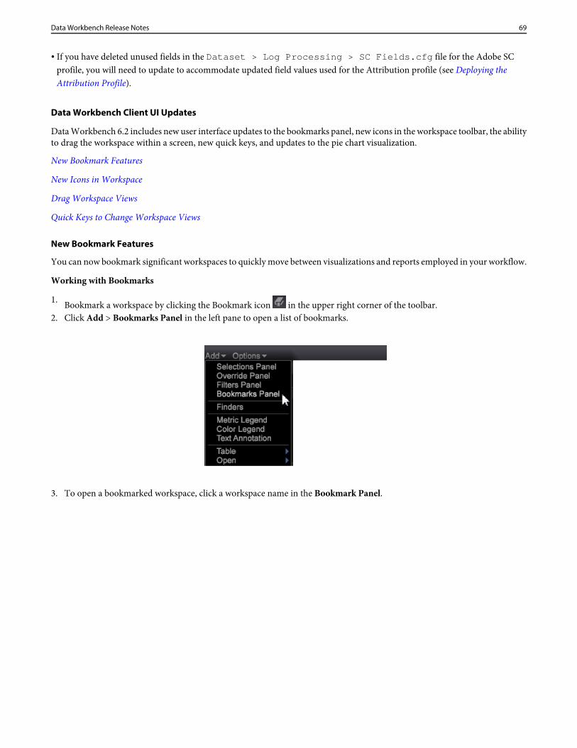
• If you have deleted unused fields in the Dataset > Log Processing > SC Fields.cfg file for the Adobe SCprofile, you will need to update to accommodate updated field values used for the Attribution profile (see Deploying theAttribution Profile).
Data Workbench Client UI Updates
Data Workbench 6.2 includes new user interface updates to the bookmarks panel, new icons in the workspace toolbar, the abilityto drag the workspace within a screen, new quick keys, and updates to the pie chart visualization.
New Bookmark Features
New Icons in Workspace
Drag Workspace Views
Quick Keys to Change Workspace Views
New Bookmark Features
You can now bookmark significant workspaces to quickly move between visualizations and reports employed in your workflow.
Working with Bookmarks
1. Bookmark a workspace by clicking the Bookmark icon in the upper right corner of the toolbar.2. Click Add > Bookmarks Panel in the left pane to open a list of bookmarks.
3. To open a bookmarked workspace, click a workspace name in the Bookmark Panel.
69Data Workbench Release Notes
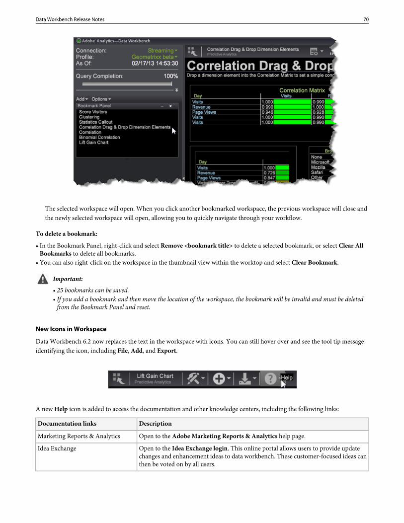
The selected workspace will open. When you click another bookmarked workspace, the previous workspace will close andthe newly selected workspace will open, allowing you to quickly navigate through your workflow.
To delete a bookmark:
• In the Bookmark Panel, right-click and select Remove <bookmark title> to delete a selected bookmark, or select Clear AllBookmarks to delete all bookmarks.
• You can also right-click on the workspace in the thumbnail view within the worktop and select Clear Bookmark.
Important:• 25 bookmarks can be saved.• If you add a bookmark and then move the location of the workspace, the bookmark will be invalid and must be deleted
from the Bookmark Panel and reset.
New Icons in Workspace
Data Workbench 6.2 now replaces the text in the workspace with icons. You can still hover over and see the tool tip messageidentifying the icon, including File, Add, and Export.
A new Help icon is added to access the documentation and other knowledge centers, including the following links:
DescriptionDocumentation links
Open to the Adobe Marketing Reports & Analytics help page.Marketing Reports & Analytics
Open to the Idea Exchange login. This online portal allows users to provide updatechanges and enhancement ideas to data workbench. These customer-focused ideas canthen be voted on by all users.
Idea Exchange
70Data Workbench Release Notes
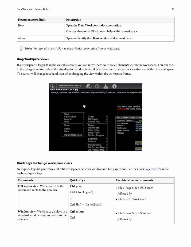
DescriptionDocumentation links
Open the Data Workbench documentation.
You can also press <F1> to open help within a workspace.
Help
Open to identify the client version of data workbench.About
Note: You can also press <F1> to open the documentation from a workspace.
Drag Workspace Views
If a workspace is larger than the viewable screen, you can move the view to see all elements within the workspace. You can clickin the background (outside of the visualizations and tables) and drag the screen to move the viewable area within the workspace.The cursor will change to a hand icon when dragging the view within the workspace frame.
Quick Keys to Change Workspace Views
New quick keys let you resize and refit workspaces between window and full page views. See the Quick Reference for morekeyboard quick keys.
Combined menu commandsQuick KeysCommands
Ctrl plus
Ctrl + (on keypad)
Full screen view. Workspace fills thescreen and refits to the new size.
• File > Page Size > Fill Screen
followed byor • File > Refit Workspace
Ctrl Shift + (on keyboard)
Ctrl minus
Ctrl -
Window view. Workspace displays in astandard window view and refits to thenew size.
• File > Page Size > Standard
followed by
71Data Workbench Release Notes
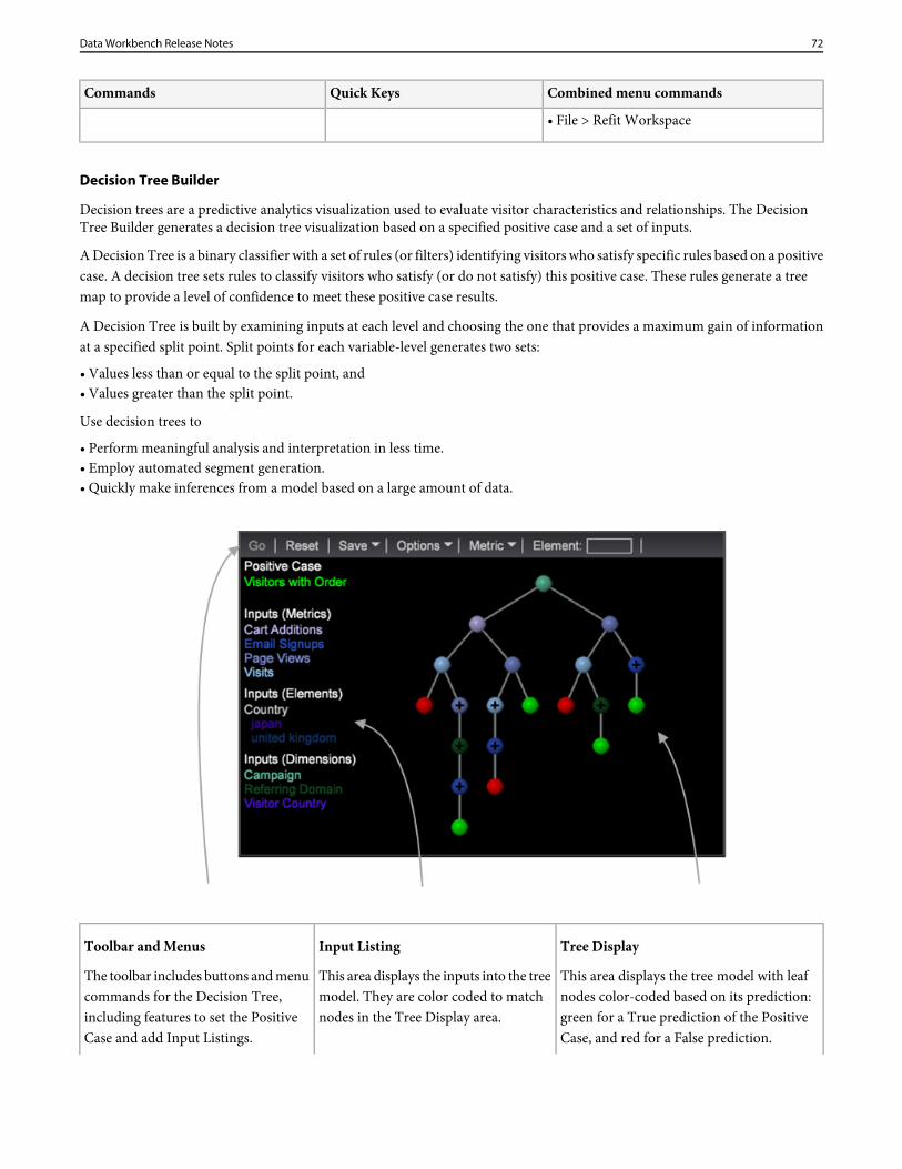
Combined menu commandsQuick KeysCommands
• File > Refit Workspace
Decision Tree Builder
Decision trees are a predictive analytics visualization used to evaluate visitor characteristics and relationships. The DecisionTree Builder generates a decision tree visualization based on a specified positive case and a set of inputs.
A Decision Tree is a binary classifier with a set of rules (or filters) identifying visitors who satisfy specific rules based on a positivecase. A decision tree sets rules to classify visitors who satisfy (or do not satisfy) this positive case. These rules generate a treemap to provide a level of confidence to meet these positive case results.
A Decision Tree is built by examining inputs at each level and choosing the one that provides a maximum gain of informationat a specified split point. Split points for each variable-level generates two sets:
• Values less than or equal to the split point, and• Values greater than the split point.
Use decision trees to
• Perform meaningful analysis and interpretation in less time.• Employ automated segment generation.• Quickly make inferences from a model based on a large amount of data.
Tree DisplayInput ListingToolbar and Menus
This area displays the tree model with leafnodes color-coded based on its prediction:
This area displays the inputs into the treemodel. They are color coded to matchnodes in the Tree Display area.
The toolbar includes buttons and menucommands for the Decision Tree,including features to set the PositiveCase and add Input Listings.
green for a True prediction of the PositiveCase, and red for a False prediction.
72Data Workbench Release Notes
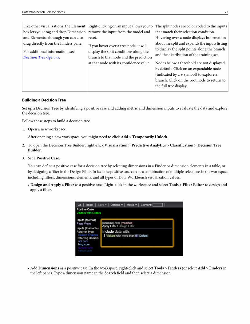
Right-clicking on an input allows you toremove the input from the model andreset.
Like other visualizations, the Elementbox lets you drag and drop Dimensionand Elements, although you can alsodrag directly from the Finders pane.
The split nodes are color coded to the inputsthat match their selection condition.Hovering over a node displays informationabout the split and expands the inputs listingIf you hover over a tree node, it will
display the split conditions along theFor additional information, seeDecision Tree Options.
to display the split points along the branchand the distribution of the training set.
Nodes below a threshold are not displayedby default. Click on an expandable node
branch to that node and the predictionat that node with its confidence value.
(indicated by a + symbol) to explore abranch. Click on the root node to return tothe full tree display.
Building a Decision Tree
Set up a Decision Tree by identifying a positive case and adding metric and dimension inputs to evaluate the data and explorethe decision tree.
Follow these steps to build a decision tree.
1. Open a new workspace.
After opening a new workspace, you might need to click Add > Temporarily Unlock.
2. To open the Decision Tree Builder, right-click Visualization > Predictive Analytics > Classification > Decision TreeBuilder.
3. Set a Positive Case.
You can define a positive case for a decision tree by selecting dimensions in a Finder or dimension elements in a table, orby designing a filter in the Design Filter. In fact, the positive case can be a combination of multiple selections in the workspaceincluding filters, dimensions, elements, and all types of Data Workbench visualization values.
• Design and Apply a Filter as a positive case. Right-click in the workspace and select Tools > Filter Editor to design andapply a filter.
• Add Dimensions as a positive case. In the workspace, right-click and select Tools > Finders (or select Add > Finders inthe left pane). Type a dimension name in the Search field and then select a dimension.
73Data Workbench Release Notes
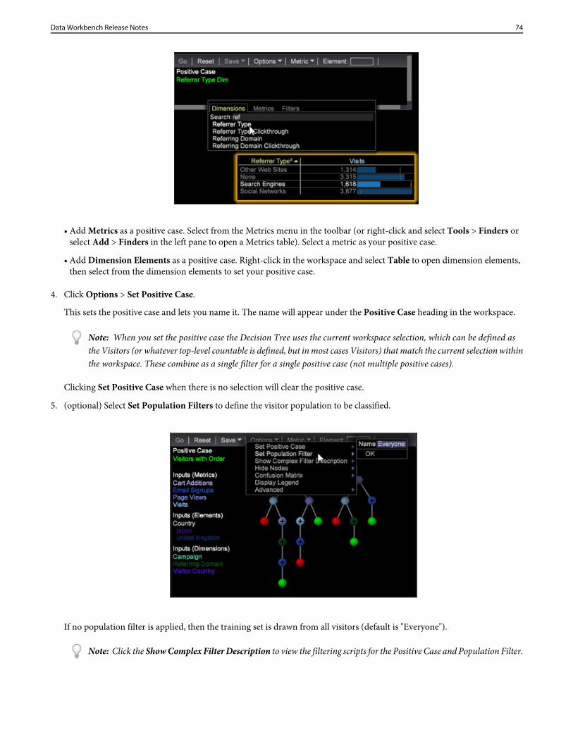
• Add Metrics as a positive case. Select from the Metrics menu in the toolbar (or right-click and select Tools > Finders orselect Add > Finders in the left pane to open a Metrics table). Select a metric as your positive case.
• Add Dimension Elements as a positive case. Right-click in the workspace and select Table to open dimension elements,then select from the dimension elements to set your positive case.
4. Click Options > Set Positive Case.
This sets the positive case and lets you name it. The name will appear under the Positive Case heading in the workspace.
Note: When you set the positive case the Decision Tree uses the current workspace selection, which can be defined asthe Visitors (or whatever top-level countable is defined, but in most cases Visitors) that match the current selection withinthe workspace. These combine as a single filter for a single positive case (not multiple positive cases).
Clicking Set Positive Case when there is no selection will clear the positive case.
5. (optional) Select Set Population Filters to define the visitor population to be classified.
If no population filter is applied, then the training set is drawn from all visitors (default is "Everyone").
Note: Click the Show Complex Filter Description to view the filtering scripts for the Positive Case and Population Filter.
74Data Workbench Release Notes
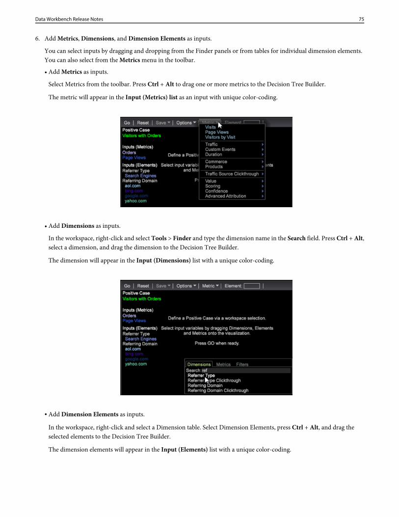
6. Add Metrics, Dimensions, and Dimension Elements as inputs.
You can select inputs by dragging and dropping from the Finder panels or from tables for individual dimension elements.You can also select from the Metrics menu in the toolbar.
• Add Metrics as inputs.
Select Metrics from the toolbar. Press Ctrl + Alt to drag one or more metrics to the Decision Tree Builder.
The metric will appear in the Input (Metrics) list as an input with unique color-coding.
• Add Dimensions as inputs.
In the workspace, right-click and select Tools > Finder and type the dimension name in the Search field. Press Ctrl + Alt,select a dimension, and drag the dimension to the Decision Tree Builder.
The dimension will appear in the Input (Dimensions) list with a unique color-coding.
• Add Dimension Elements as inputs.
In the workspace, right-click and select a Dimension table. Select Dimension Elements, press Ctrl + Alt, and drag theselected elements to the Decision Tree Builder.
The dimension elements will appear in the Input (Elements) list with a unique color-coding.
75Data Workbench Release Notes
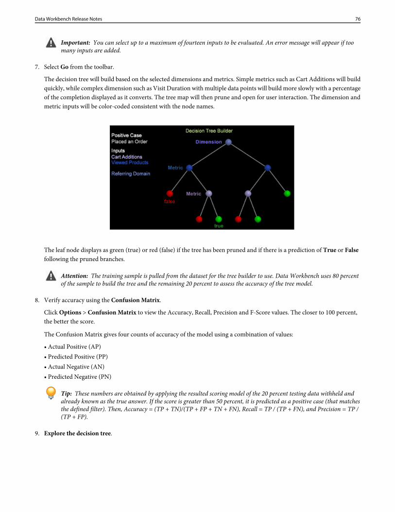
Important: You can select up to a maximum of fourteen inputs to be evaluated. An error message will appear if toomany inputs are added.
7. Select Go from the toolbar.
The decision tree will build based on the selected dimensions and metrics. Simple metrics such as Cart Additions will buildquickly, while complex dimension such as Visit Duration with multiple data points will build more slowly with a percentageof the completion displayed as it converts. The tree map will then prune and open for user interaction. The dimension andmetric inputs will be color-coded consistent with the node names.
The leaf node displays as green (true) or red (false) if the tree has been pruned and if there is a prediction of True or Falsefollowing the pruned branches.
Attention: The training sample is pulled from the dataset for the tree builder to use. Data Workbench uses 80 percentof the sample to build the tree and the remaining 20 percent to assess the accuracy of the tree model.
8. Verify accuracy using the Confusion Matrix.
Click Options > Confusion Matrix to view the Accuracy, Recall, Precision and F-Score values. The closer to 100 percent,the better the score.
The Confusion Matrix gives four counts of accuracy of the model using a combination of values:
• Actual Positive (AP)• Predicted Positive (PP)• Actual Negative (AN)• Predicted Negative (PN)
Tip: These numbers are obtained by applying the resulted scoring model of the 20 percent testing data withheld andalready known as the true answer. If the score is greater than 50 percent, it is predicted as a positive case (that matchesthe defined filter). Then, Accuracy = (TP + TN)/(TP + FP + TN + FN), Recall = TP / (TP + FN), and Precision = TP /(TP + FP).
9. Explore the decision tree.
76Data Workbench Release Notes
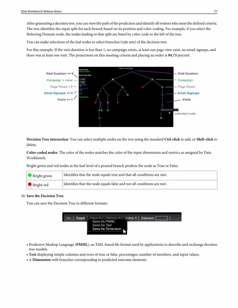
After generating a decision tree, you can view the path of the prediction and identify all visitors who meet the defined criteria.The tree identifies the input split for each branch based on its position and color-coding. For example, if you select theReferring Domain node, the nodes leading to that split are listed by color-code to the left of the tree.
You can make selections of the leaf nodes to select branches (rule sets) of the decision tree.
For this example: If the visit duration is less than 1, no campaign exists, at least one page view exist, no email signups, andthere was at least one visit. The projections on this meeting criteria and placing an order is 94.73 percent.
Decision Tree interaction: You can select multiple nodes on the tree using the standard Ctrl-click to add, or Shift-click todelete.
Color-coded nodes: The color of the nodes matches the color of the input dimensions and metrics as assigned by DataWorkbench.
Bright green and red nodes at the leaf-level of a pruned branch predicts the node as True or False.
Identifies that the node equals true and that all conditions are met. Bright green
Identifies that the node equals false and not all conditions are met. Bright red
10. Save the Decision Tree.
You can save the Decision Tree in different formats:
• Predictive Markup Language (PMML), an XML-based file format used by applications to describe and exchange decisiontree models.
• Text displaying simple columns and rows of true or false, percentages, number of members, and input values.• A Dimension with branches corresponding to predicted outcome elements.
77Data Workbench Release Notes
Decision Tree Options
The Decision Tree menu includes features to set the positive use case, filters, leaf distribution options, confusion matrix, andother advanced options.
DescriptionToolbar buttons
Click to run the decision tree algorithm and display the visualization. This is grayed-outuntil there are inputs.
Go
Clears inputs and decision tree model and resets the process.Reset
Save the Decision Tree. You can save the Decision Tree in different formats:Save
• Predictive Markup Language (PMML), an XML-based file format used by applicationsto describe and exchange decision tree models.
• Text displaying simple columns and rows of true or false, percentages, number ofmembers, and input values.
• A Dimension with branches corresponding to predicted outcome elements.
See table below for Options menu.Options
Lists Metrics that can be added to the modelMetric
Drag and drop Dimensions and Elements to this box (or directly to the visualization).Element
DescriptionOptions menu
Defines the current workspace selection as the model's Positive Case. Clears the caseif no selection exists.
Set Positive Case
Defines the current workspace selection as the model's Population Filter and will bedrawn from visitors who satisfy this condition. The default is "Everyone."
Set Population Filter
Displays descriptions of the defined filters. Click to view the filtering scripts for thePositive Case and Population Filter.
Show Complex Filter Description
Hides nodes with only a small percentage of the population. This menu commanddisplays only when the decision tree is displayed.
Hide Nodes
Click Options > Confusion Matrix to view the Accuracy, Recall, Precision and F-Scorevalues. The closer to 100 percent, the better the score.
Confusion Matrix
The Confusion Matrix gives four counts of accuracy of the model using a combinationof values:
• Actual Positive (AP)• Predicted Positive (PP)• Actual Negative (AN)• Predicted Negative (PN)
Tip: These numbers are obtained by applying the resulted scoring model of the20 percent testing data withheld and already known as the true answer. If the scoreis greater than 50 percent, it is predicted as a positive case (that matches the definedfilter). Then, Accuracy = (TP + TN)/(TP + FP + TN + FN), Recall = TP / (TP +FN), and Precision = TP / (TP + FP).
78Data Workbench Release Notes
DescriptionOptions menu
Allows you to toggle a legend key on and off in the Decision Tree.Display Legend
This menu command displays only when the decision tree is displayed.
Click to open Advanced menu for in-depth use of Decision Tree. See table below formenu options.
Advanced
DescriptionAdvanced menu
Controls the size of the training set used for the model building. Larger sets take longerto train, smaller sets take less time.
Training Set Size
Allows the user to specify whether to use the Min-Max or the Z Score technique tonormalize inputs into the model.
Input Normalization
When the Positive Case does not occur very often (less than 10 percent) in the trainingsample, SMOTE is used to provide additional samples. This option allows the user toindicate how many more samples to create using SMOTE.
SMOTE Over-Sampling Factor
Allows you to set the threshold assumed for a leaf during the tree building process. Bydefault, all members of a node must be identical for it to be a leaf (prior to pruningstage).
Leaf Class Distribution Threshold
Finders
Use Finder panels in Data Workbench to select metrics, dimensions, and filters. These panels provide search support, sortingoptions, and drag and drop capabilities.
A Finder panel can be opened in the left sidebar or within a workspace.
79Data Workbench Release Notes
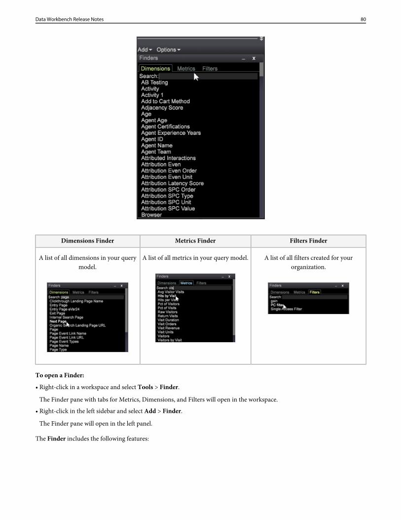
Filters FinderMetrics FinderDimensions Finder
A list of all filters created for yourorganization.
A list of all metrics in your query model.A list of all dimensions in your querymodel.
To open a Finder:
• Right-click in a workspace and select Tools > Finder.
The Finder pane with tabs for Metrics, Dimensions, and Filters will open in the workspace.
• Right-click in the left sidebar and select Add > Finder.
The Finder pane will open in the left panel.
The Finder includes the following features:
80Data Workbench Release Notes
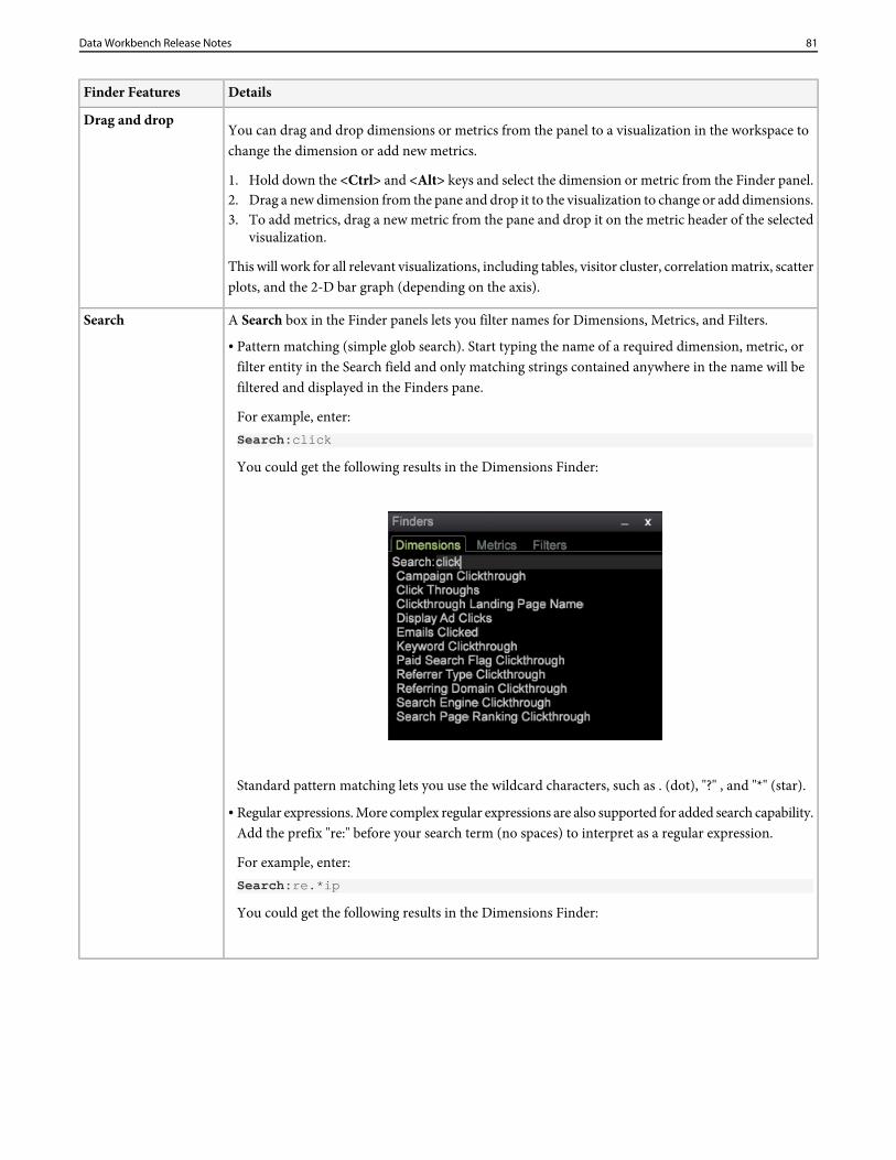
DetailsFinder Features
You can drag and drop dimensions or metrics from the panel to a visualization in the workspace tochange the dimension or add new metrics.
Drag and drop
1. Hold down the <Ctrl> and <Alt> keys and select the dimension or metric from the Finder panel.2. Drag a new dimension from the pane and drop it to the visualization to change or add dimensions.3. To add metrics, drag a new metric from the pane and drop it on the metric header of the selected
visualization.
This will work for all relevant visualizations, including tables, visitor cluster, correlation matrix, scatterplots, and the 2-D bar graph (depending on the axis).
A Search box in the Finder panels lets you filter names for Dimensions, Metrics, and Filters.Search• Pattern matching (simple glob search). Start typing the name of a required dimension, metric, or
filter entity in the Search field and only matching strings contained anywhere in the name will befiltered and displayed in the Finders pane.
For example, enter:Search:click
You could get the following results in the Dimensions Finder:
Standard pattern matching lets you use the wildcard characters, such as . (dot), "?" , and "*" (star).
• Regular expressions. More complex regular expressions are also supported for added search capability.Add the prefix "re:" before your search term (no spaces) to interpret as a regular expression.
For example, enter:Search:re.*ip
You could get the following results in the Dimensions Finder:
81Data Workbench Release Notes
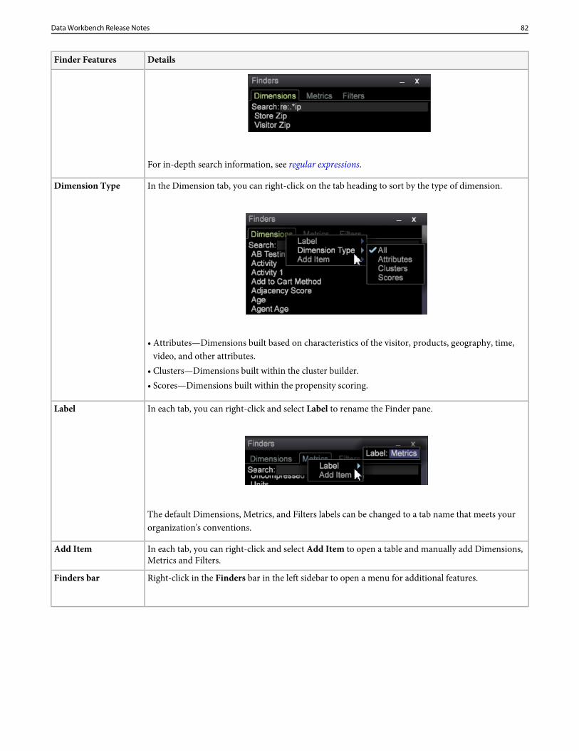
DetailsFinder Features
For in-depth search information, see regular expressions.
In the Dimension tab, you can right-click on the tab heading to sort by the type of dimension.Dimension Type
• Attributes—Dimensions built based on characteristics of the visitor, products, geography, time,video, and other attributes.
• Clusters—Dimensions built within the cluster builder.• Scores—Dimensions built within the propensity scoring.
In each tab, you can right-click and select Label to rename the Finder pane.Label
The default Dimensions, Metrics, and Filters labels can be changed to a tab name that meets yourorganization's conventions.
In each tab, you can right-click and select Add Item to open a table and manually add Dimensions,Metrics and Filters.
Add Item
Right-click in the Finders bar in the left sidebar to open a menu for additional features.Finders bar
82Data Workbench Release Notes
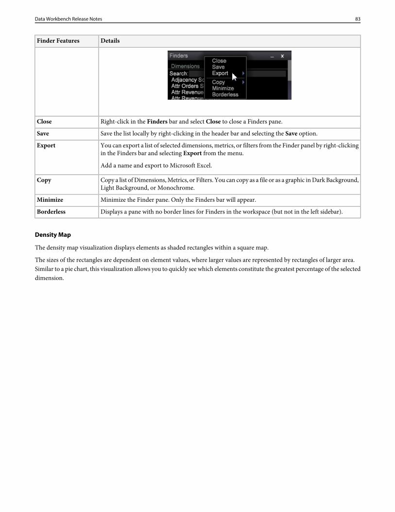
DetailsFinder Features
Right-click in the Finders bar and select Close to close a Finders pane.Close
Save the list locally by right-clicking in the header bar and selecting the Save option.Save
You can export a list of selected dimensions, metrics, or filters from the Finder panel by right-clickingin the Finders bar and selecting Export from the menu.
Add a name and export to Microsoft Excel.
Export
Copy a list of Dimensions, Metrics, or Filters. You can copy as a file or as a graphic in Dark Background,Light Background, or Monochrome.
Copy
Minimize the Finder pane. Only the Finders bar will appear.Minimize
Displays a pane with no border lines for Finders in the workspace (but not in the left sidebar).Borderless
Density Map
The density map visualization displays elements as shaded rectangles within a square map.
The sizes of the rectangles are dependent on element values, where larger values are represented by rectangles of larger area.Similar to a pie chart, this visualization allows you to quickly see which elements constitute the greatest percentage of the selecteddimension.
83Data Workbench Release Notes
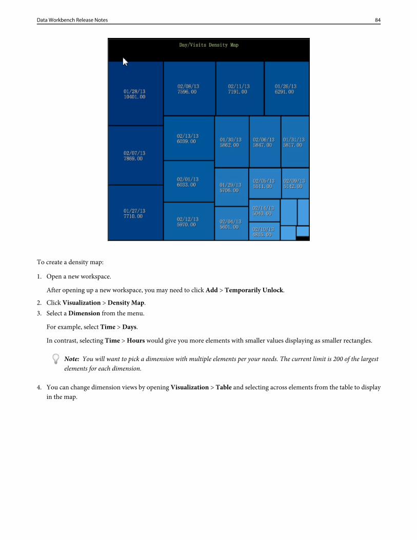
To create a density map:
1. Open a new workspace.
After opening up a new workspace, you may need to click Add > Temporarily Unlock.
2. Click Visualization > Density Map.3. Select a Dimension from the menu.
For example, select Time > Days.
In contrast, selecting Time > Hours would give you more elements with smaller values displaying as smaller rectangles.
Note: You will want to pick a dimension with multiple elements per your needs. The current limit is 200 of the largestelements for each dimension.
4. You can change dimension views by opening Visualization > Table and selecting across elements from the table to displayin the map.
84Data Workbench Release Notes
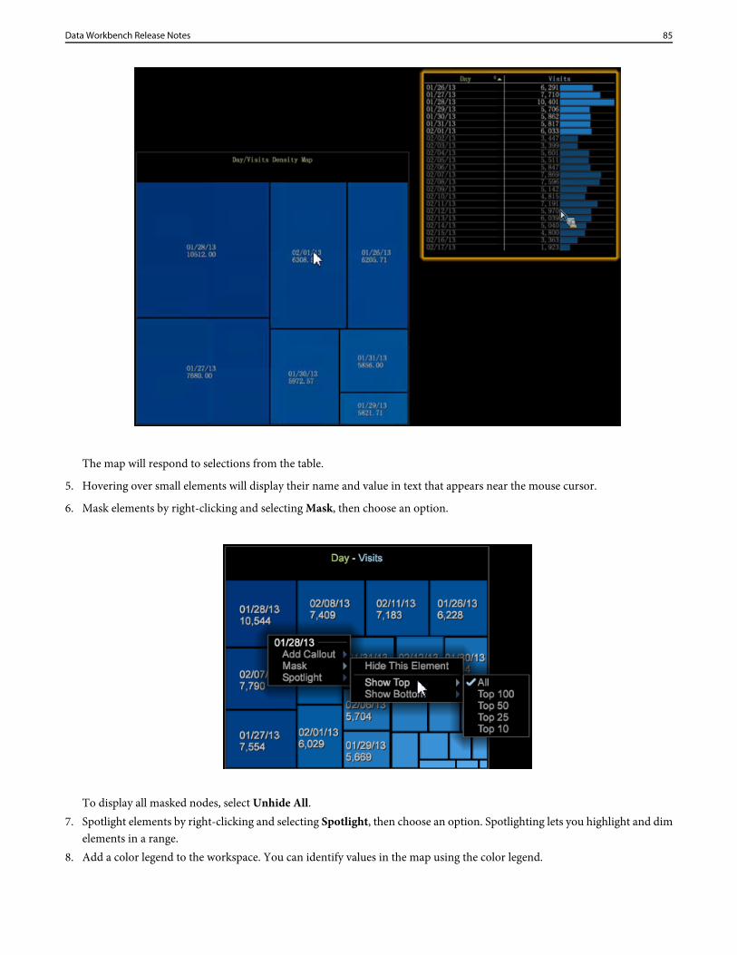
The map will respond to selections from the table.
5. Hovering over small elements will display their name and value in text that appears near the mouse cursor.
6. Mask elements by right-clicking and selecting Mask, then choose an option.
To display all masked nodes, select Unhide All.7. Spotlight elements by right-clicking and selecting Spotlight, then choose an option. Spotlighting lets you highlight and dim
elements in a range.8. Add a color legend to the workspace. You can identify values in the map using the color legend.
85Data Workbench Release Notes
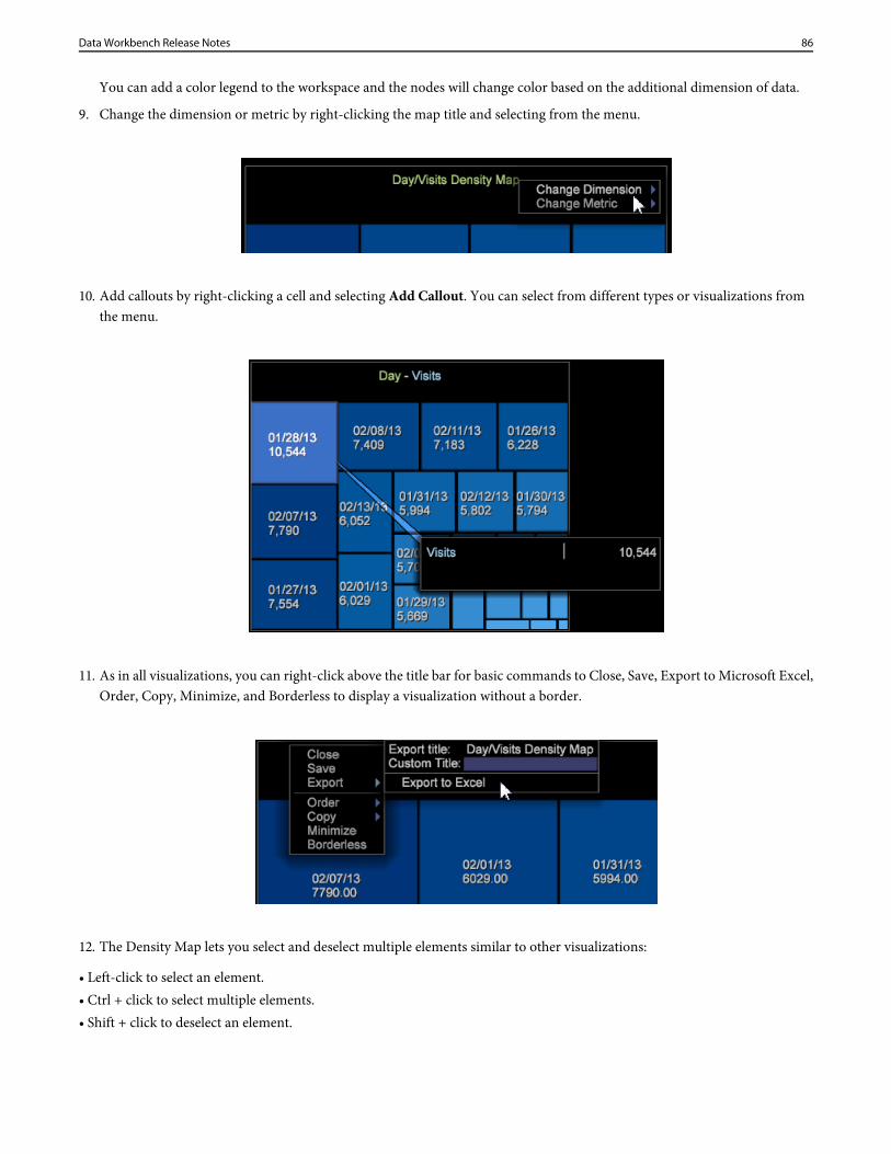
You can add a color legend to the workspace and the nodes will change color based on the additional dimension of data.
9. Change the dimension or metric by right-clicking the map title and selecting from the menu.
10. Add callouts by right-clicking a cell and selecting Add Callout. You can select from different types or visualizations fromthe menu.
11. As in all visualizations, you can right-click above the title bar for basic commands to Close, Save, Export to Microsoft Excel,Order, Copy, Minimize, and Borderless to display a visualization without a border.
12. The Density Map lets you select and deselect multiple elements similar to other visualizations:
• Left-click to select an element.• Ctrl + click to select multiple elements.• Shift + click to deselect an element.
86Data Workbench Release Notes
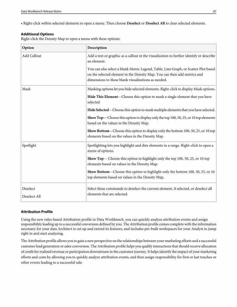
• Right-click within selected elements to open a menu. Then choose Deselect or Deselect All to clear selected elements.
Additional OptionsRight-click the Density Map to open a menu with these options:
DescriptionOption
Add a text or graphic as a callout in the visualization to further identify or describean element.
You can also select a blank Metric Legend, Table, Line Graph, or Scatter Plot basedon the selected element in the Density Map. You can then add metrics anddimensions to these blank visualizations as needed.
Add Callout
Masking options let you hide selected elements. Right-click to display Mask options.
Hide This Element—Choose this option to mask a single element that you haveselected.
Mask
Hide Selected—Choose this option to mask multiple elements that you have selected.
Show Top— Choose this option to display only the top 100, 50, 25, or 10 top elementsbased on the values in the Density Map.
Show Bottom—Choose this option to display only the bottom 100, 50, 25, or 10 topelements based on the values in the Density Map.
Spotlighting lets you highlight and dim elements in a range. Right-click to open amenu of options.
Show Top— Choose this option to highlight only the top 100, 50, 25, or 10 topelements based on values in the Density Map.
Spotlight
Show Bottom—Choose this option to highlight only the bottom 100, 50, 25, or 10top elements based on values in the Density Map.
Select these commands to deselect the current element, if selected, or deselect allelements that are selected.
Deselect
Deselect All
Attribution Profile
Using the new rules-based Attribution profile in Data Workbench, you can quickly analyze attribution events and assignresponsibility leading up to a successful conversion defined by you. The Attribution profile comes complete with the informationnecessary for your data Architect to set up and extend its features, and includes pre-built workspaces for your Analyst to jumpright in and start analyzing.
The Attribution profile allows you to gain a new perspective on the relationships between your marketing efforts and a successfulcustomer lead generation or sales conversion. The Attribution profile helps you qualify interactions that should receive allocationof credit for realized revenue or participation downstream in the customer journey. It helps identify the impact of your marketingefforts and costs by allowing you to quickly analyze attribution events, and then assign responsibility for first or last touches orother events leading to a successful sale.
87Data Workbench Release Notes
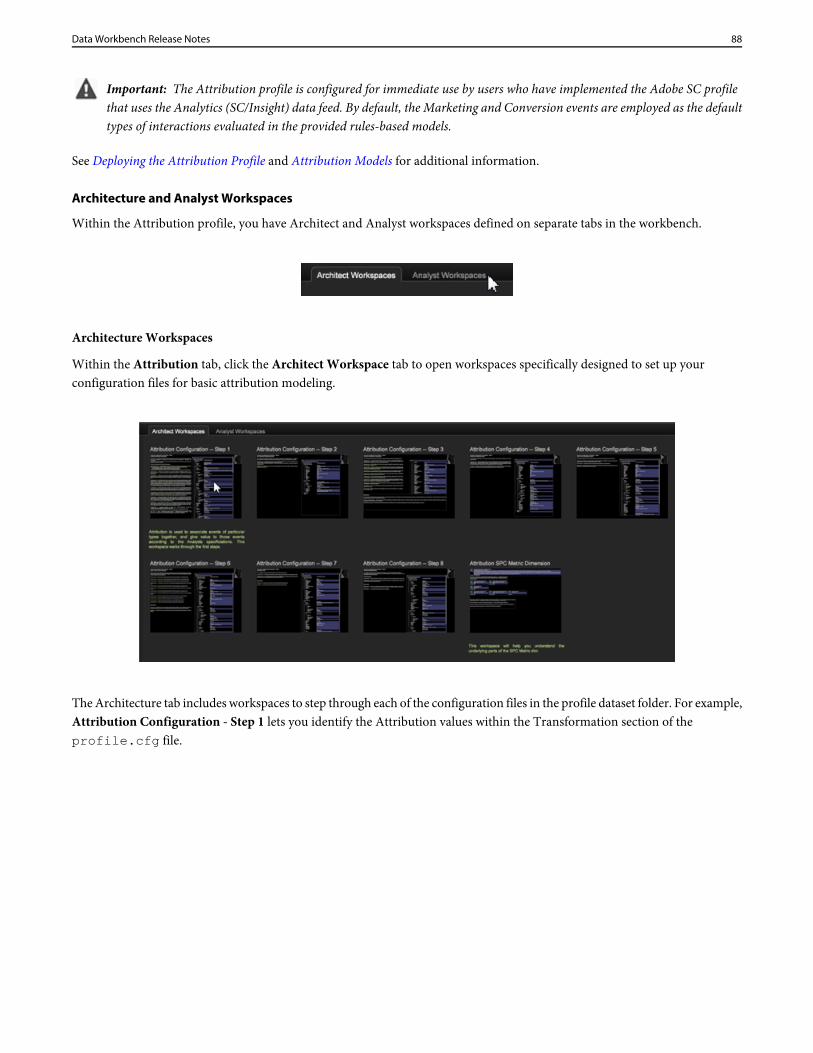
Important: The Attribution profile is configured for immediate use by users who have implemented the Adobe SC profilethat uses the Analytics (SC/Insight) data feed. By default, the Marketing and Conversion events are employed as the defaulttypes of interactions evaluated in the provided rules-based models.
See Deploying the Attribution Profile and Attribution Models for additional information.
Architecture and Analyst Workspaces
Within the Attribution profile, you have Architect and Analyst workspaces defined on separate tabs in the workbench.
Architecture Workspaces
Within the Attribution tab, click the Architect Workspace tab to open workspaces specifically designed to set up yourconfiguration files for basic attribution modeling.
The Architecture tab includes workspaces to step through each of the configuration files in the profile dataset folder. For example,Attribution Configuration - Step 1 lets you identify the Attribution values within the Transformation section of theprofile.cfg file.
88Data Workbench Release Notes
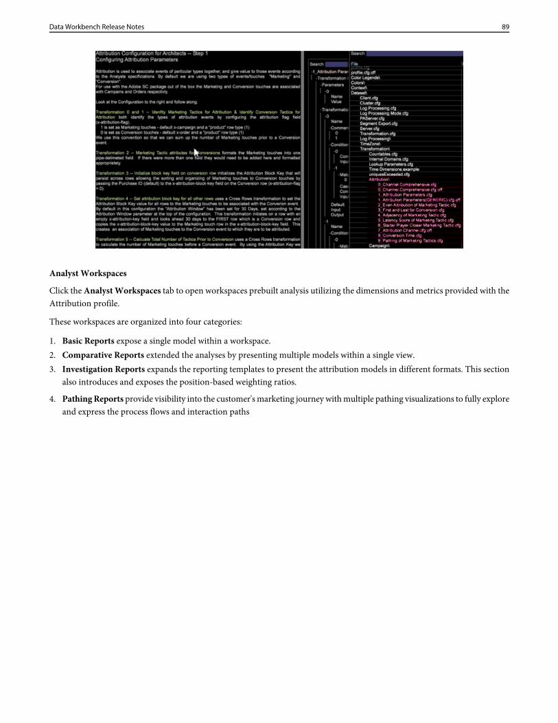
Analyst Workspaces
Click the Analyst Workspaces tab to open workspaces prebuilt analysis utilizing the dimensions and metrics provided with theAttribution profile.
These workspaces are organized into four categories:
1. Basic Reports expose a single model within a workspace.2. Comparative Reports extended the analyses by presenting multiple models within a single view.3. Investigation Reports expands the reporting templates to present the attribution models in different formats. This section
also introduces and exposes the position-based weighting ratios.
4. Pathing Reports provide visibility into the customer's marketing journey with multiple pathing visualizations to fully exploreand express the process flows and interaction paths
89Data Workbench Release Notes
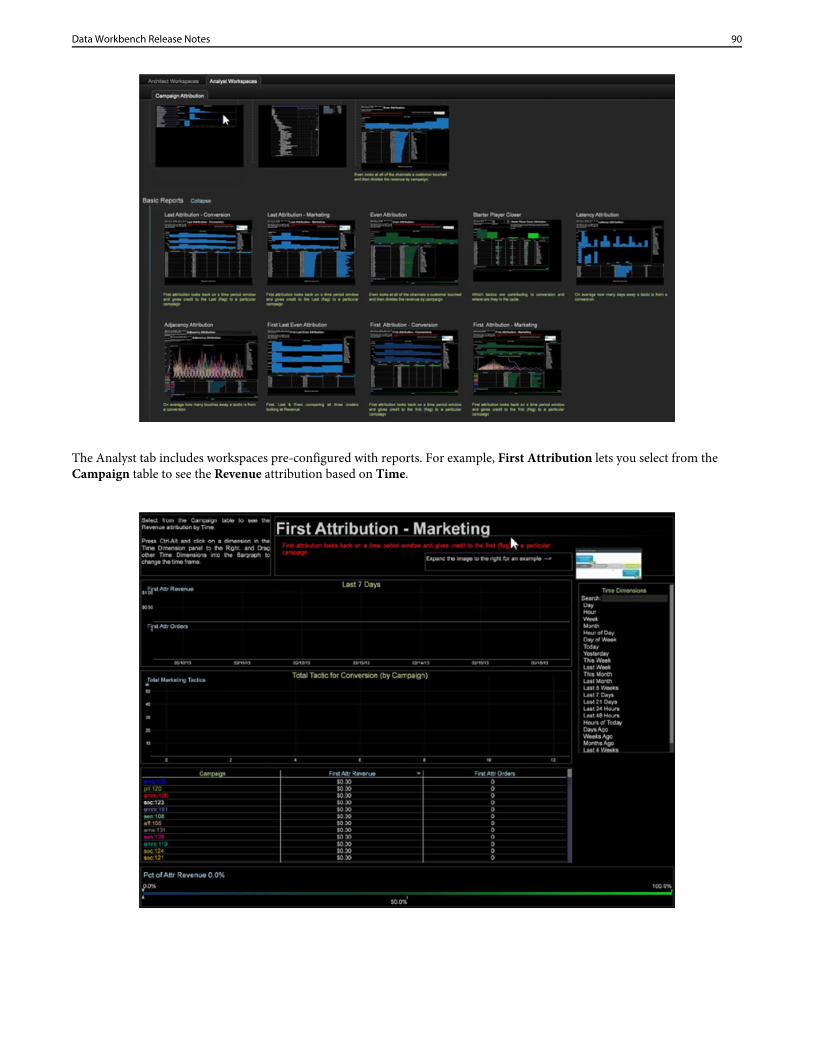
The Analyst tab includes workspaces pre-configured with reports. For example, First Attribution lets you select from theCampaign table to see the Revenue attribution based on Time.
90Data Workbench Release Notes
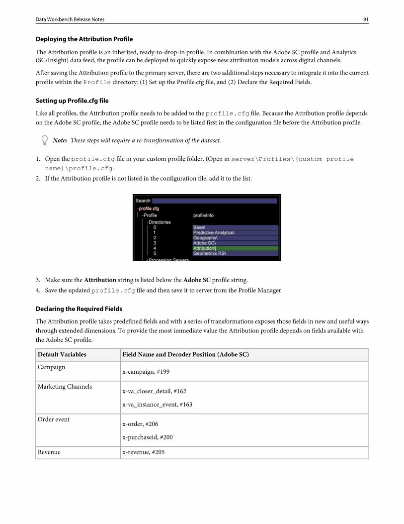
Deploying the Attribution Profile
The Attribution profile is an inherited, ready-to-drop-in profile. In combination with the Adobe SC profile and Analytics(SC/Insight) data feed, the profile can be deployed to quickly expose new attribution models across digital channels.
After saving the Attribution profile to the primary server, there are two additional steps necessary to integrate it into the currentprofile within the Profile directory: (1) Set up the Profile.cfg file, and (2) Declare the Required Fields.
Setting up Profile.cfg file
Like all profiles, the Attribution profile needs to be added to the profile.cfg file. Because the Attribution profile dependson the Adobe SC profile, the Adobe SC profile needs to be listed first in the configuration file before the Attribution profile.
Note: These steps will require a re-transformation of the dataset.
1. Open the profile.cfg file in your custom profile folder. (Open in server\Profiles\(custom profilename)\profile.cfg.
2. If the Attribution profile is not listed in the configuration file, add it to the list.
3. Make sure the Attribution string is listed below the Adobe SC profile string.4. Save the updated profile.cfg file and then save it to server from the Profile Manager.
Declaring the Required Fields
The Attribution profile takes predefined fields and with a series of transformations exposes those fields in new and useful waysthrough extended dimensions. To provide the most immediate value the Attribution profile depends on fields available withthe Adobe SC profile.
Field Name and Decoder Position (Adobe SC)Default Variables
x-campaign, #199Campaign
x-va_closer_detail, #162Marketing Channels
x-va_instance_event, #163
x-order, #206Order event
x-purchaseid, #200
x-revenue, #205Revenue
91Data Workbench Release Notes
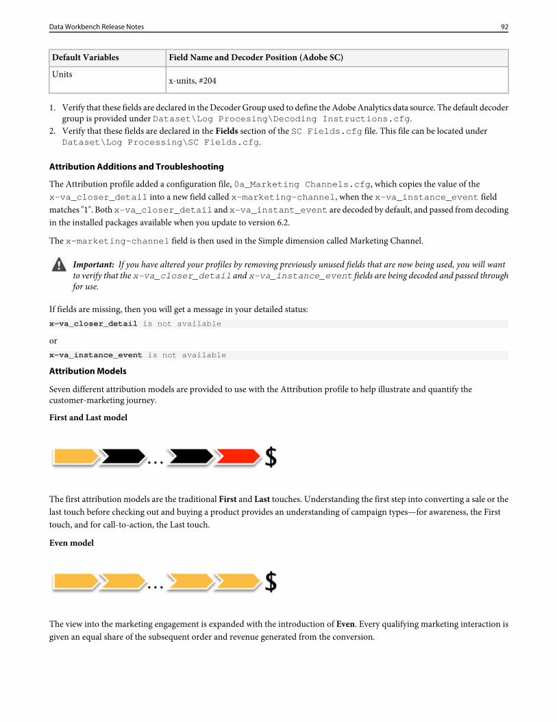
Field Name and Decoder Position (Adobe SC)Default Variables
x-units, #204Units
1. Verify that these fields are declared in the Decoder Group used to define the Adobe Analytics data source. The default decodergroup is provided under Dataset\Log Procesing\Decoding Instructions.cfg.
2. Verify that these fields are declared in the Fields section of the SC Fields.cfg file. This file can be located underDataset\Log Processing\SC Fields.cfg.
Attribution Additions and Troubleshooting
The Attribution profile added a configuration file, 0a_Marketing Channels.cfg, which copies the value of thex-va_closer_detail into a new field called x-marketing-channel, when the x-va_instance_event fieldmatches "1". Both x-va_closer_detail and x-va_instant_event are decoded by default, and passed from decodingin the installed packages available when you update to version 6.2.
The x-marketing-channel field is then used in the Simple dimension called Marketing Channel.
Important: If you have altered your profiles by removing previously unused fields that are now being used, you will wantto verify that the x-va_closer_detail and x-va_instance_event fields are being decoded and passed throughfor use.
If fields are missing, then you will get a message in your detailed status:x-va_closer_detail is not available
orx-va_instance_event is not available
Attribution Models
Seven different attribution models are provided to use with the Attribution profile to help illustrate and quantify thecustomer-marketing journey.
First and Last model
The first attribution models are the traditional First and Last touches. Understanding the first step into converting a sale or thelast touch before checking out and buying a product provides an understanding of campaign types—for awareness, the Firsttouch, and for call-to-action, the Last touch.
Even model
The view into the marketing engagement is expanded with the introduction of Even. Every qualifying marketing interaction isgiven an equal share of the subsequent order and revenue generated from the conversion.
92Data Workbench Release Notes
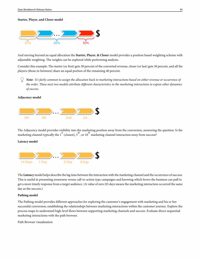
Starter, Player, and Closer model
And moving beyond an equal allocation the Starter, Player, & Closer model provides a position based weighting scheme withadjustable weighting. The weights can be explored while performing analysis.
Consider this example: The starter (or first) gets 30 percent of the converted revenue, closer (or last) gets 30 percent, and all theplayers (those in-between) share an equal portion of the remaining 40 percent.
Note: It's fairly common to assign the allocation back to marketing interactions based on either revenue or occurrence ofthe order. These next two models attribute different characteristics to the marketing interactions to expose other dynamicsof success.
Adjacency model
The Adjacency model provides visibility into the marketing position away from the conversion, answering the question: Is themarketing channel typically the 1
st (closest), 5
th, or 10
th marketing channel interaction away from success?
Latency model
The Latency model helps describe the lag time between the interaction with the marketing channel and the occurrence of success.This is useful in presenting awareness versus call-to-action type campaigns and knowing which levers the business can pull toget a more timely response from a target audience. (A value of zero (0) days means the marketing interaction occurred the sameday as the success.)
Pathing model
The Pathing model provides different approaches for exploring the customer's engagement with marketing and his or hersuccessful conversion, establishing the relationships between marketing interactions within the customer journey. Explore theprocess maps to understand high-level flows between supporting marketing channels and success. Evaluate direct sequentialmarketing interactions with the path browser.
Path Browser visualization
93Data Workbench Release Notes
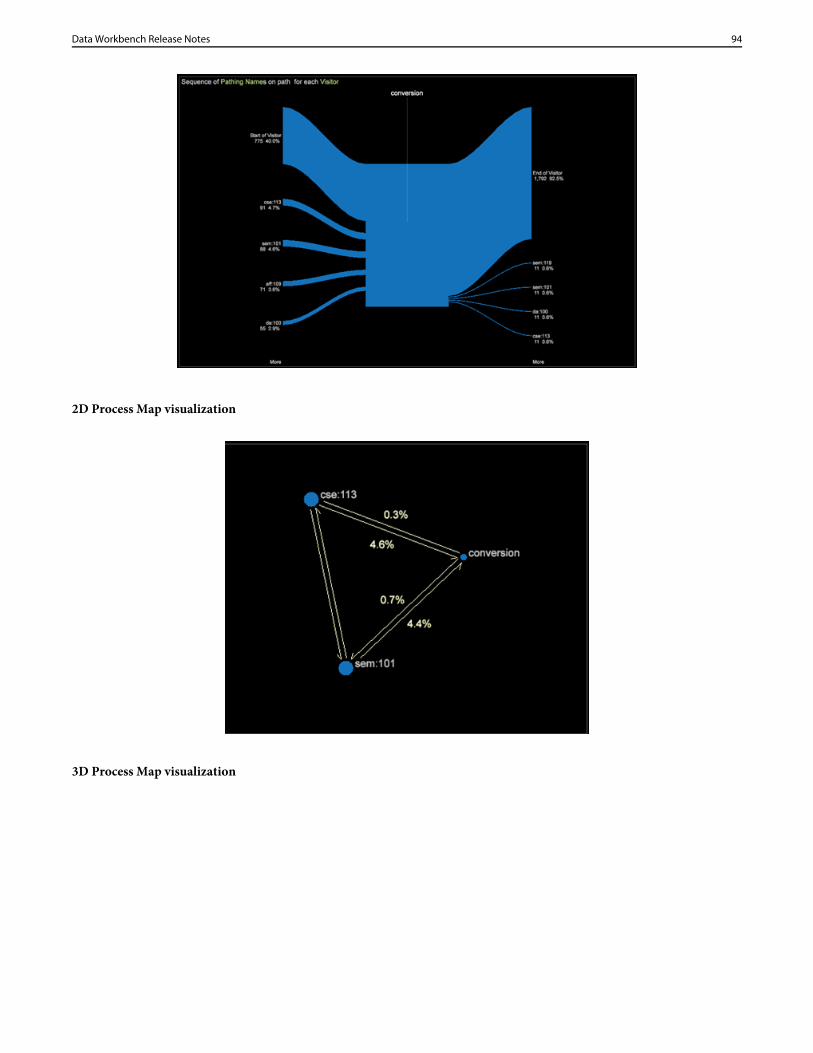
2D Process Map visualization
3D Process Map visualization
94Data Workbench Release Notes
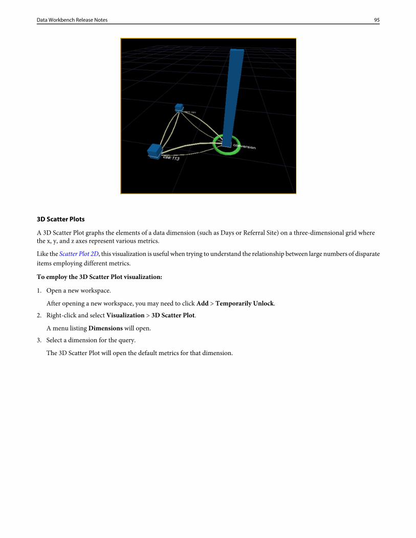
3D Scatter Plots
A 3D Scatter Plot graphs the elements of a data dimension (such as Days or Referral Site) on a three-dimensional grid wherethe x, y, and z axes represent various metrics.
Like the Scatter Plot 2D, this visualization is useful when trying to understand the relationship between large numbers of disparateitems employing different metrics.
To employ the 3D Scatter Plot visualization:
1. Open a new workspace.
After opening a new workspace, you may need to click Add > Temporarily Unlock.
2. Right-click and select Visualization > 3D Scatter Plot.
A menu listing Dimensions will open.
3. Select a dimension for the query.
The 3D Scatter Plot will open the default metrics for that dimension.
95Data Workbench Release Notes
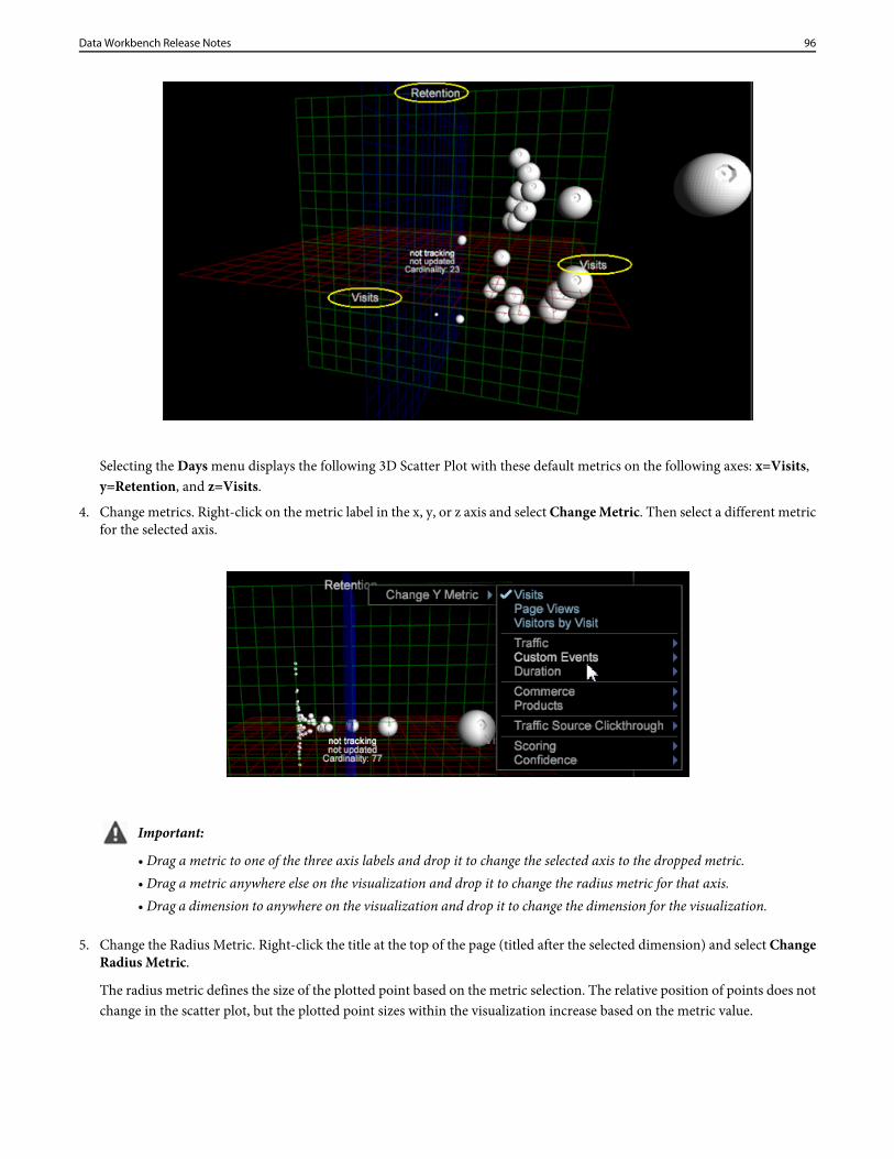
Selecting the Days menu displays the following 3D Scatter Plot with these default metrics on the following axes: x=Visits,y=Retention, and z=Visits.
4. Change metrics. Right-click on the metric label in the x, y, or z axis and select Change Metric. Then select a different metricfor the selected axis.
Important:
• Drag a metric to one of the three axis labels and drop it to change the selected axis to the dropped metric.• Drag a metric anywhere else on the visualization and drop it to change the radius metric for that axis.• Drag a dimension to anywhere on the visualization and drop it to change the dimension for the visualization.
5. Change the Radius Metric. Right-click the title at the top of the page (titled after the selected dimension) and select ChangeRadius Metric.
The radius metric defines the size of the plotted point based on the metric selection. The relative position of points does notchange in the scatter plot, but the plotted point sizes within the visualization increase based on the metric value.
96Data Workbench Release Notes
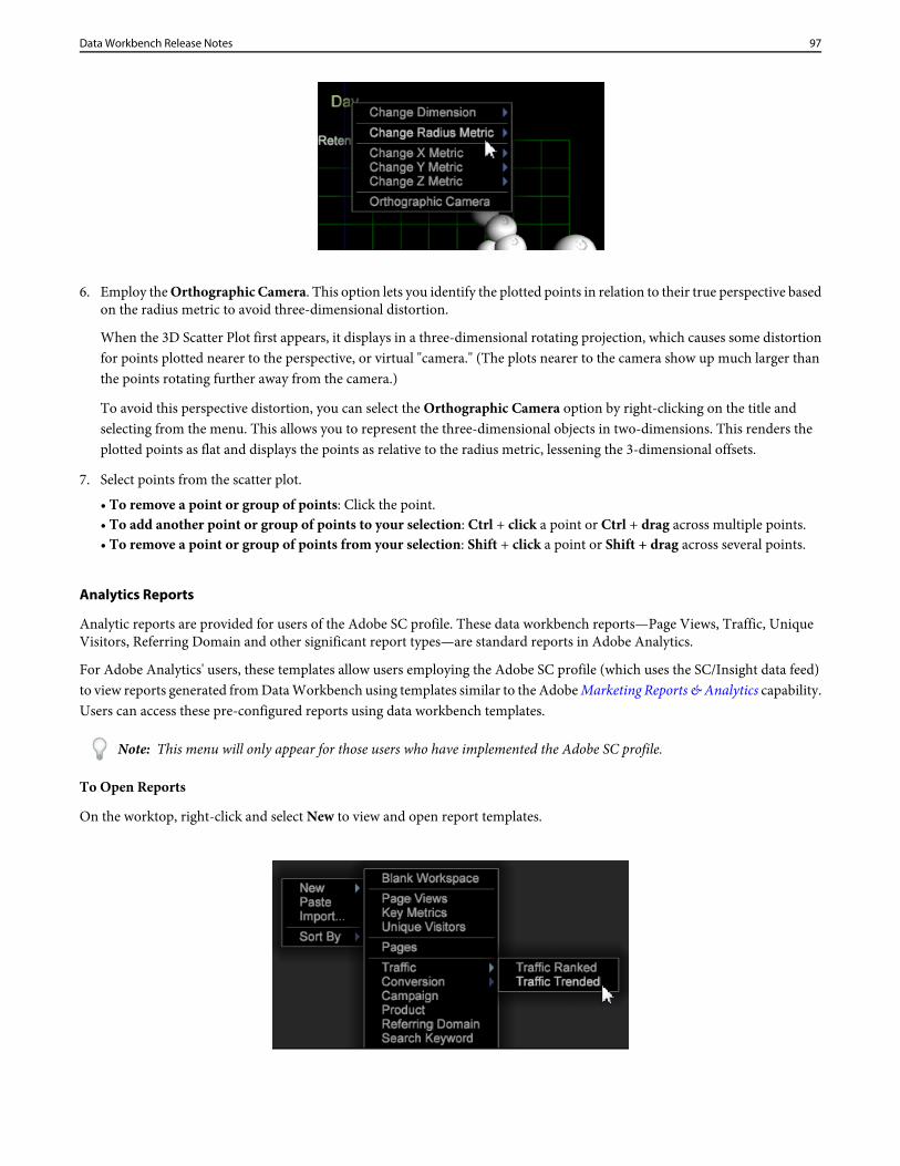
6. Employ the Orthographic Camera. This option lets you identify the plotted points in relation to their true perspective basedon the radius metric to avoid three-dimensional distortion.
When the 3D Scatter Plot first appears, it displays in a three-dimensional rotating projection, which causes some distortionfor points plotted nearer to the perspective, or virtual "camera." (The plots nearer to the camera show up much larger thanthe points rotating further away from the camera.)
To avoid this perspective distortion, you can select the Orthographic Camera option by right-clicking on the title andselecting from the menu. This allows you to represent the three-dimensional objects in two-dimensions. This renders theplotted points as flat and displays the points as relative to the radius metric, lessening the 3-dimensional offsets.
7. Select points from the scatter plot.
• To remove a point or group of points: Click the point.• To add another point or group of points to your selection: Ctrl + click a point or Ctrl + drag across multiple points.• To remove a point or group of points from your selection: Shift + click a point or Shift + drag across several points.
Analytics Reports
Analytic reports are provided for users of the Adobe SC profile. These data workbench reports—Page Views, Traffic, UniqueVisitors, Referring Domain and other significant report types—are standard reports in Adobe Analytics.
For Adobe Analytics' users, these templates allow users employing the Adobe SC profile (which uses the SC/Insight data feed)to view reports generated from Data Workbench using templates similar to the Adobe Marketing Reports & Analytics capability.Users can access these pre-configured reports using data workbench templates.
Note: This menu will only appear for those users who have implemented the Adobe SC profile.
To Open Reports
On the worktop, right-click and select New to view and open report templates.
97Data Workbench Release Notes
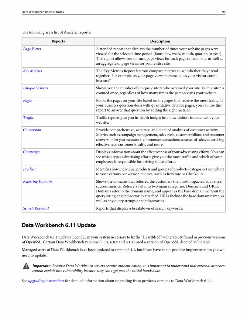
The following are a list of Analytic reports:
DescriptionReports
A trended report that displays the number of times your website pages wereviewed for the selected time period (hour, day, week, month, quarter, or year).
Page Views
This report allows you to track page views for each page on your site, as well asan aggregate of page views for your entire site.
The Key Metrics Report lets you compare metrics to see whether they trendtogether. For example, as your page views increase, does your visitor countincrease?
Key Metrics
Shows you the number of unique visitors who accessed your site. Each visitor iscounted once, regardless of how many times the person visits your website.
Unique Visitors
Ranks the pages on your site based on the pages that receive the most traffic. Ifyour business question deals with quantitative data for pages, you can use thisreport to answer that question by adding the right metrics.
Pages
Traffic reports give you in-depth insight into how visitors interact with yourwebsite.
Traffic
Provide comprehensive, accurate, and detailed analysis of customer activity.Metrics such as campaign management, sales cycle, customer fallout, and customer
Conversion
conversion let you measure e-commerce transactions, sources of sales, advertisingeffectiveness, customer loyalty, and more.
Displays information about the effectiveness of your advertising efforts. You cansee which types advertising efforts give you the most traffic and which of youremployees is responsible for driving those efforts.
Campaign
Identifies how individual products and groups of products (categories) contributeto your various conversion metrics, such as Revenue or Checkouts.
Product
Shows the domains that referred the customers that most impacted your site'ssuccess metrics. Referrers fall into two main categories: Domains and URLs.
Referring Domain
Domains refer to the domain name, and appear as the base domain without thequery string or subdirectories attached. URLs include the base domain name, aswell as any query strings or subdirectories.
Reports that display a breakdown of search keywords.Search Keyword
Data Workbench 6.11 Update
Data Workbench 6.1.1 updates OpenSSL in your system necessary to fix the "Heartbleed" vulnerability found in previous versionsof OpenSSL. Certain Data Workbench versions (5.5.x, 6.0.x and 6.1.x) used a version of OpenSSL deemed vulnerable.
Managed users of Data Workbench have been updated to version 6.1.1, but if you have an on-premise implementation you willneed to update.
Important: Because Data Workbench servers require authentication, it is important to understand that external attackerscannot exploit this vulnerability because they can't get past the initial handshake.
See upgrading instructions for detailed information about upgrading from previous versions to Data Workbench 6.1.1.
98Data Workbench Release Notes
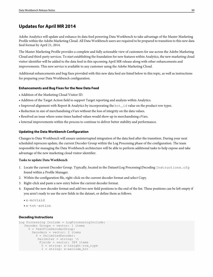
Updates for April MR 2014
Adobe Analytics will update and enhance its data feed powering Data Workbench to take advantage of the Master MarketingProfile within the Adobe Marketing Cloud. All Data Workbench users are required to be prepared to transition to this new datafeed format by April 21, 2014.
The Master Marketing Profile provides a complete and fully actionable view of customers for use across the Adobe MarketingCloud and third-party services. To start establishing the foundation for new features within Analytics, the new marketing cloudvisitor identifier will be added to the data feed in this upcoming April MR release along with other enhancements andimprovements. This new service is available to any customer using the Adobe Marketing Cloud.
Additional enhancements and bug fixes provided with this new data feed are listed below in this topic, as well as instructionsfor preparing your Data Workbench configuration.
Enhancements and Bug Fixes for the New Data Feed
• Addition of the Marketing Cloud Visitor ID.• Addition of the Target Action field to support Target reporting and analysis within Analytics.• Improved alignment with Report & Analytics by incorporating the bot_id value on the product row types.• Reduction in size of merchandising eVars without the loss of integrity on the data values.• Resolved an issue where some times hashed values would show up in merchandising eVars.• Internal improvements within the process to continue to deliver better stability and performance.
Updating the Data Workbench Configuration
Changes to Data Workbench will ensure uninterrupted integration of the data feed after the transition. During your nextscheduled reprocess update, the current Decoder Group within the Log Processing phase of the configuration. The teamresponsible for managing the Data Workbench architecture will be able to perform additional tasks to help expose and takeadvantage of the new marketing cloud visitor identifier.
Tasks to update Data Workbench
1. Locate the current Decoder Group. Typically, located in the Dataset\Log Processing\Decoding Instructions.cfgfound within a Profile Manager.
2. Within the configuration file, right-click on the current decoder format and select Copy.3. Right-click and paste a new entry below the current decoder format.4. Expand the new decoder format and add two new field positions to the end of the list. These positions can be left empty if
you aren't ready to use the new fields in the dataset, or define them as follows.
• x-mcvisid• x-tnt-action
Decoding InstructionsLog Processing Include = LogProcessingInclude: Decoder Groups = vector: 1 items 0 = TextFileDecoderGroup: Decoders = vector: 2 items 0 = DelimitedDecoder: Delimiter = string: \t Fields = vector: 389 items 0 = string: x-insight-row_type 1 = string: x-exclude_hit
99Data Workbench Release Notes
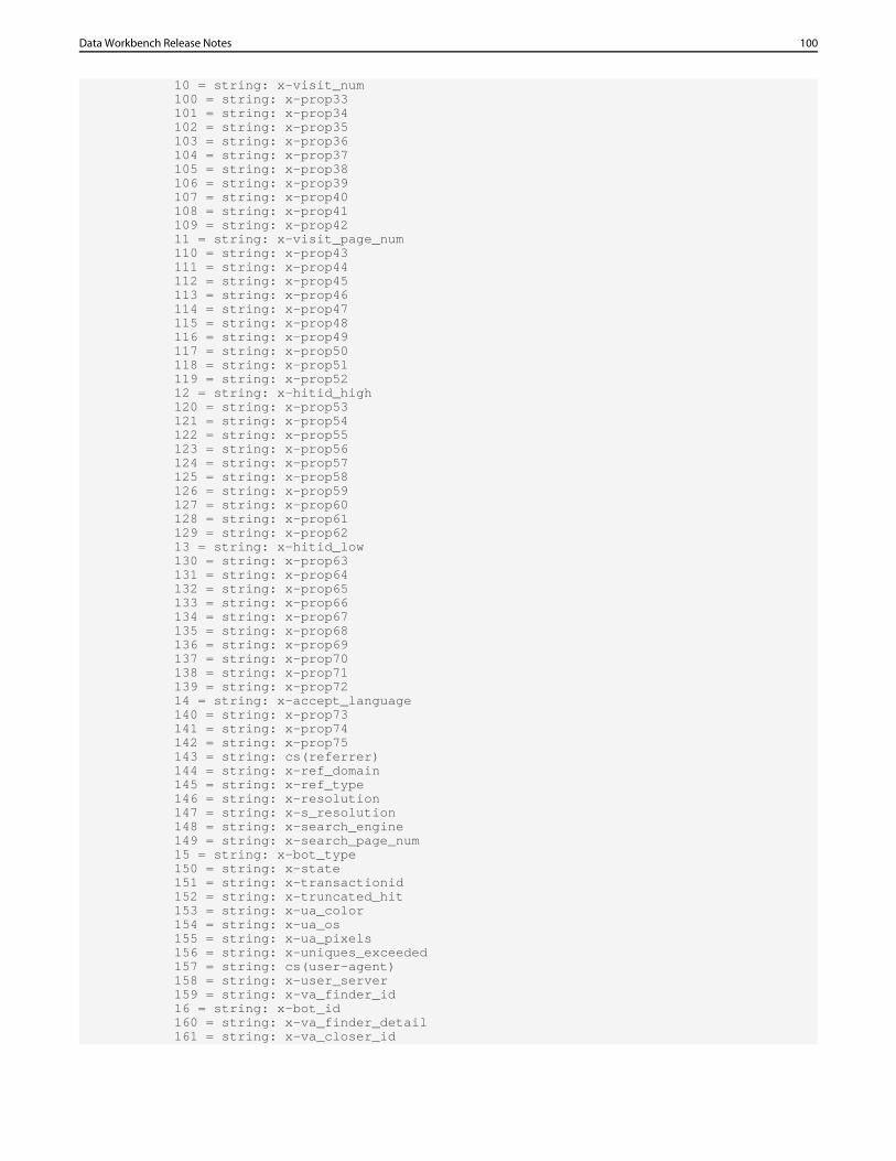
10 = string: x-visit_num 100 = string: x-prop33 101 = string: x-prop34 102 = string: x-prop35 103 = string: x-prop36 104 = string: x-prop37 105 = string: x-prop38 106 = string: x-prop39 107 = string: x-prop40 108 = string: x-prop41 109 = string: x-prop42 11 = string: x-visit_page_num 110 = string: x-prop43 111 = string: x-prop44 112 = string: x-prop45 113 = string: x-prop46 114 = string: x-prop47 115 = string: x-prop48 116 = string: x-prop49 117 = string: x-prop50 118 = string: x-prop51 119 = string: x-prop52 12 = string: x-hitid_high 120 = string: x-prop53 121 = string: x-prop54 122 = string: x-prop55 123 = string: x-prop56 124 = string: x-prop57 125 = string: x-prop58 126 = string: x-prop59 127 = string: x-prop60 128 = string: x-prop61 129 = string: x-prop62 13 = string: x-hitid_low 130 = string: x-prop63 131 = string: x-prop64 132 = string: x-prop65 133 = string: x-prop66 134 = string: x-prop67 135 = string: x-prop68 136 = string: x-prop69 137 = string: x-prop70 138 = string: x-prop71 139 = string: x-prop72 14 = string: x-accept_language 140 = string: x-prop73 141 = string: x-prop74 142 = string: x-prop75 143 = string: cs(referrer) 144 = string: x-ref_domain 145 = string: x-ref_type 146 = string: x-resolution 147 = string: x-s_resolution 148 = string: x-search_engine 149 = string: x-search_page_num 15 = string: x-bot_type 150 = string: x-state 151 = string: x-transactionid 152 = string: x-truncated_hit 153 = string: x-ua_color 154 = string: x-ua_os 155 = string: x-ua_pixels 156 = string: x-uniques_exceeded 157 = string: cs(user-agent) 158 = string: x-user_server 159 = string: x-va_finder_id 16 = string: x-bot_id 160 = string: x-va_finder_detail 161 = string: x-va_closer_id
100Data Workbench Release Notes
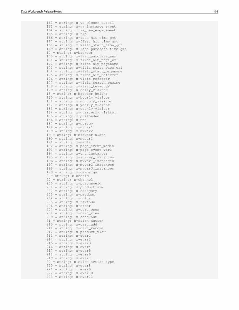
162 = string: x-va_closer_detail 163 = string: x-va_instance_event 164 = string: x-va_new_engagement 165 = string: x-zip 166 = string: x-last_hit_time_gmt 167 = string: x-first_hit_time_gmt 168 = string: x-visit_start_time_gmt 169 = string: x-last_purchase_time_gmt 17 = string: x-browser 170 = string: x-last_purchase_num 171 = string: x-first_hit_page_url 172 = string: x-first_hit_pagename 173 = string: x-visit_start_page_url 174 = string: x-visit_start_pagename 175 = string: x-first_hit_referrer 176 = string: x-visit_referrer 177 = string: x-visit_search_engine 178 = string: x-visit_keywords 179 = string: x-daily_visitor 18 = string: x-browser_height 180 = string: x-hourly_visitor 181 = string: x-monthly_visitor 182 = string: x-yearly_visitor 183 = string: x-weekly_visitor 184 = string: x-quarterly_visitor 185 = string: x-preloaded 186 = string: x-tnt 187 = string: x-survey 188 = string: x-mvvar1 189 = string: x-mvvar2 19 = string: x-browser_width 190 = string: x-mvvar3 191 = string: x-media 192 = string: x-page_event_media 193 = string: x-page_event_var3 194 = string: x-tnt_instances 195 = string: x-survey_instances 196 = string: x-mvvar1_instances 197 = string: x-mvvar2_instances 198 = string: x-mvvar3_instances 199 = string: x-campaign 2 = string: x-userid 20 = string: x-channel 200 = string: x-purchaseid 201 = string: x-product-num 202 = string: x-category 203 = string: x-product 204 = string: x-units 205 = string: x-revenue 206 = string: x-order 207 = string: x-cart_open 208 = string: x-cart_view 209 = string: x-checkout 21 = string: x-click_action 210 = string: x-cart_add 211 = string: x-cart_remove 212 = string: x-product_view 213 = string: x-evar1 214 = string: x-evar2 215 = string: x-evar3 216 = string: x-evar4 217 = string: x-evar5 218 = string: x-evar6 219 = string: x-evar7 22 = string: x-click_action_type 220 = string: x-evar8 221 = string: x-evar9 222 = string: x-evar10 223 = string: x-evar11
101Data Workbench Release Notes
224 = string: x-evar12 225 = string: x-evar13 226 = string: x-evar14 227 = string: x-evar15 228 = string: x-evar16 229 = string: x-evar17 23 = string: x-click_context 230 = string: x-evar18 231 = string: x-evar19 232 = string: x-evar20 233 = string: x-evar21 234 = string: x-evar22 235 = string: x-evar23 236 = string: x-evar24 237 = string: x-evar25 238 = string: x-evar26 239 = string: x-evar27 24 = string: x-click_context_type 240 = string: x-evar28 241 = string: x-evar29 242 = string: x-evar30 243 = string: x-evar31 244 = string: x-evar32 245 = string: x-evar33 246 = string: x-evar34 247 = string: x-evar35 248 = string: x-evar36 249 = string: x-evar37 25 = string: x-click_source_id 250 = string: x-evar38 251 = string: x-evar39 252 = string: x-evar40 253 = string: x-evar41 254 = string: x-evar42 255 = string: x-evar43 256 = string: x-evar44 257 = string: x-evar45 258 = string: x-evar46 259 = string: x-evar47 26 = string: x-click_tag 260 = string: x-evar48 261 = string: x-evar49 262 = string: x-evar50 263 = string: x-evar51 264 = string: x-evar52 265 = string: x-evar53 266 = string: x-evar54 267 = string: x-evar55 268 = string: x-evar56 269 = string: x-evar57 27 = string: x-code_ver 270 = string: x-evar58 271 = string: x-evar59 272 = string: x-evar60 273 = string: x-evar61 274 = string: x-evar62 275 = string: x-evar63 276 = string: x-evar64 277 = string: x-evar65 278 = string: x-evar66 279 = string: x-evar67 28 = string: x-c_color 280 = string: x-evar68 281 = string: x-evar69 282 = string: x-evar70 283 = string: x-evar71 284 = string: x-evar72 285 = string: x-evar73 286 = string: x-evar74
102Data Workbench Release Notes
287 = string: x-evar75 288 = string: x-cust1 289 = string: x-cust2 29 = string: x-color 290 = string: x-cust3 291 = string: x-cust4 292 = string: x-cust5 293 = string: x-cust6 294 = string: x-cust7 295 = string: x-cust8 296 = string: x-cust9 297 = string: x-cust10 298 = string: x-cust11 299 = string: x-cust12 3 = string: x-service 30 = string: x-cookies 300 = string: x-cust13 301 = string: x-cust14 302 = string: x-cust15 303 = string: x-cust16 304 = string: x-cust17 305 = string: x-cust18 306 = string: x-cust19 307 = string: x-cust20 308 = string: x-cust21 309 = string: x-cust22 31 = string: x-ct_connect_type 310 = string: x-cust23 311 = string: x-cust24 312 = string: x-cust25 313 = string: x-cust26 314 = string: x-cust27 315 = string: x-cust28 316 = string: x-cust29 317 = string: x-cust30 318 = string: x-cust31 319 = string: x-cust32 32 = string: x-connection_type 320 = string: x-cust33 321 = string: x-cust34 322 = string: x-cust35 323 = string: x-cust36 324 = string: x-cust37 325 = string: x-cust38 326 = string: x-cust39 327 = string: x-cust40 328 = string: x-cust41 329 = string: x-cust42 33 = string: x-country 330 = string: x-cust43 331 = string: x-cust44 332 = string: x-cust45 333 = string: x-cust46 334 = string: x-cust47 335 = string: x-cust48 336 = string: x-cust49 337 = string: x-cust50 338 = string: x-cust51 339 = string: x-cust52 34 = string: x-currency 340 = string: x-cust53 341 = string: x-cust54 342 = string: x-cust55 343 = string: x-cust56 344 = string: x-cust57 345 = string: x-cust58 346 = string: x-cust59 347 = string: x-cust60 348 = string: x-cust61
103Data Workbench Release Notes
349 = string: x-cust62 35 = string: x-curr_rate 350 = string: x-cust63 351 = string: x-cust64 352 = string: x-cust65 353 = string: x-cust66 354 = string: x-cust67 355 = string: x-cust68 356 = string: x-cust69 357 = string: x-cust70 358 = string: x-cust71 359 = string: x-cust72 36 = string: x-curr_factor 360 = string: x-cust73 361 = string: x-cust74 362 = string: x-cust75 363 = string: x-cust76 364 = string: x-cust77 365 = string: x-cust78 366 = string: x-cust79 367 = string: x-cust80 368 = string: x-cust81 369 = string: x-cust82 37 = string: x-domain 370 = string: x-cust83 371 = string: x-cust84 372 = string: x-cust85 373 = string: x-cust86 374 = string: x-cust87 375 = string: x-cust88 376 = string: x-cust89 377 = string: x-cust90 378 = string: x-cust91 379 = string: x-cust92 38 = string: x-geo_city 380 = string: x-cust93 381 = string: x-cust94 382 = string: x-cust95 383 = string: x-cust96 384 = string: x-cust97 385 = string: x-cust98 386 = string: x-cust99 387 = string: x-cust100 388 = string: x-ecom_additional_data 39 = string: x-geo_country 4 = string: x-page_event 40 = string: x-geo_dma 41 = string: x-geo_region 42 = string: x-geo_zip 43 = string: x-hier1 44 = string: x-hier2 45 = string: x-hier3 46 = string: x-hier4 47 = string: x-hier5 48 = string: x-homepage 49 = string: c-ip 5 = string: x-hit_source 50 = string: x-j_jscript 51 = string: x-javascript 52 = string: x-java_enabled 53 = string: x-keywords 54 = string: x-language 55 = string: x-mobile_id 56 = string: x-new_visit 57 = string: x-os 58 = string: x-p_plugins 59 = string: x-plugins 6 = string: x-hit_time_gmt 60 = string: x-page_event_var1
104Data Workbench Release Notes
61 = string: x-page_event_var2 62 = string: x-page_type 63 = string: cs-uri 64 = string: x-pagename 65 = string: x-paid_search 66 = string: x-partner_plugins 67 = string: x-persistent_cookie 68 = string: x-prop1 69 = string: x-prop2 7 = string: x-date_time 70 = string: x-prop3 71 = string: x-prop4 72 = string: x-prop5 73 = string: x-prop6 74 = string: x-prop7 75 = string: x-prop8 76 = string: x-prop9 77 = string: x-prop10 78 = string: x-prop11 79 = string: x-prop12 8 = string: x-visid_high 80 = string: x-prop13 81 = string: x-prop14 82 = string: x-prop15 83 = string: x-prop16 84 = string: x-prop17 85 = string: x-prop18 86 = string: x-prop19 87 = string: x-prop20 88 = string: x-prop21 89 = string: x-prop22 9 = string: x-visid_low 90 = string: x-prop23 91 = string: x-prop24 92 = string: x-prop25 93 = string: x-prop26 94 = string: x-prop27 95 = string: x-prop28 96 = string: x-prop29 97 = string: x-prop30 98 = string: x-prop31 99 = string: x-prop32 1 = DelimitedDecoder: Delimiter = string: \t Fields = vector: 391 items 0 = string: x-insight-row_type 1 = string: x-exclude_hit 10 = string: x-visit_num 100 = string: x-prop33 101 = string: x-prop34 102 = string: x-prop35 103 = string: x-prop36 104 = string: x-prop37 105 = string: x-prop38 106 = string: x-prop39 107 = string: x-prop40 108 = string: x-prop41 109 = string: x-prop42 11 = string: x-visit_page_num 110 = string: x-prop43 111 = string: x-prop44 112 = string: x-prop45 113 = string: x-prop46 114 = string: x-prop47 115 = string: x-prop48 116 = string: x-prop49 117 = string: x-prop50 118 = string: x-prop51 119 = string: x-prop52
105Data Workbench Release Notes
12 = string: x-hitid_high 120 = string: x-prop53 121 = string: x-prop54 122 = string: x-prop55 123 = string: x-prop56 124 = string: x-prop57 125 = string: x-prop58 126 = string: x-prop59 127 = string: x-prop60 128 = string: x-prop61 129 = string: x-prop62 13 = string: x-hitid_low 130 = string: x-prop63 131 = string: x-prop64 132 = string: x-prop65 133 = string: x-prop66 134 = string: x-prop67 135 = string: x-prop68 136 = string: x-prop69 137 = string: x-prop70 138 = string: x-prop71 139 = string: x-prop72 14 = string: x-accept_language 140 = string: x-prop73 141 = string: x-prop74 142 = string: x-prop75 143 = string: cs(referrer) 144 = string: x-ref_domain 145 = string: x-ref_type 146 = string: x-resolution 147 = string: x-s_resolution 148 = string: x-search_engine 149 = string: x-search_page_num 15 = string: x-bot_type 150 = string: x-state 151 = string: x-transactionid 152 = string: x-truncated_hit 153 = string: x-ua_color 154 = string: x-ua_os 155 = string: x-ua_pixels 156 = string: x-uniques_exceeded 157 = string: cs(user-agent) 158 = string: x-user_server 159 = string: x-va_finder_id 16 = string: x-bot_id 160 = string: x-va_finder_detail 161 = string: x-va_closer_id 162 = string: x-va_closer_detail 163 = string: x-va_instance_event 164 = string: x-va_new_engagement 165 = string: x-zip 166 = string: x-last_hit_time_gmt 167 = string: x-first_hit_time_gmt 168 = string: x-visit_start_time_gmt 169 = string: x-last_purchase_time_gmt 17 = string: x-browser 170 = string: x-last_purchase_num 171 = string: x-first_hit_page_url 172 = string: x-first_hit_pagename 173 = string: x-visit_start_page_url 174 = string: x-visit_start_pagename 175 = string: x-first_hit_referrer 176 = string: x-visit_referrer 177 = string: x-visit_search_engine 178 = string: x-visit_keywords 179 = string: x-daily_visitor 18 = string: x-browser_height 180 = string: x-hourly_visitor 181 = string: x-monthly_visitor
106Data Workbench Release Notes
182 = string: x-yearly_visitor 183 = string: x-weekly_visitor 184 = string: x-quarterly_visitor 185 = string: x-preloaded 186 = string: x-tnt 187 = string: x-survey 188 = string: x-mvvar1 189 = string: x-mvvar2 19 = string: x-browser_width 190 = string: x-mvvar3 191 = string: x-media 192 = string: x-page_event_media 193 = string: x-page_event_var3 194 = string: x-tnt_instances 195 = string: x-survey_instances 196 = string: x-mvvar1_instances 197 = string: x-mvvar2_instances 198 = string: x-mvvar3_instances 199 = string: x-campaign 2 = string: x-userid 20 = string: x-channel 200 = string: x-purchaseid 201 = string: x-product-num 202 = string: x-category 203 = string: x-product 204 = string: x-units 205 = string: x-revenue 206 = string: x-order 207 = string: x-cart_open 208 = string: x-cart_view 209 = string: x-checkout 21 = string: x-click_action 210 = string: x-cart_add 211 = string: x-cart_remove 212 = string: x-product_view 213 = string: x-evar1 214 = string: x-evar2 215 = string: x-evar3 216 = string: x-evar4 217 = string: x-evar5 218 = string: x-evar6 219 = string: x-evar7 22 = string: x-click_action_type 220 = string: x-evar8 221 = string: x-evar9 222 = string: x-evar10 223 = string: x-evar11 224 = string: x-evar12 225 = string: x-evar13 226 = string: x-evar14 227 = string: x-evar15 228 = string: x-evar16 229 = string: x-evar17 23 = string: x-click_context 230 = string: x-evar18 231 = string: x-evar19 232 = string: x-evar20 233 = string: x-evar21 234 = string: x-evar22 235 = string: x-evar23 236 = string: x-evar24 237 = string: x-evar25 238 = string: x-evar26 239 = string: x-evar27 24 = string: x-click_context_type 240 = string: x-evar28 241 = string: x-evar29 242 = string: x-evar30 243 = string: x-evar31
107Data Workbench Release Notes
244 = string: x-evar32 245 = string: x-evar33 246 = string: x-evar34 247 = string: x-evar35 248 = string: x-evar36 249 = string: x-evar37 25 = string: x-click_source_id 250 = string: x-evar38 251 = string: x-evar39 252 = string: x-evar40 253 = string: x-evar41 254 = string: x-evar42 255 = string: x-evar43 256 = string: x-evar44 257 = string: x-evar45 258 = string: x-evar46 259 = string: x-evar47 26 = string: x-click_tag 260 = string: x-evar48 261 = string: x-evar49 262 = string: x-evar50 263 = string: x-evar51 264 = string: x-evar52 265 = string: x-evar53 266 = string: x-evar54 267 = string: x-evar55 268 = string: x-evar56 269 = string: x-evar57 27 = string: x-code_ver 270 = string: x-evar58 271 = string: x-evar59 272 = string: x-evar60 273 = string: x-evar61 274 = string: x-evar62 275 = string: x-evar63 276 = string: x-evar64 277 = string: x-evar65 278 = string: x-evar66 279 = string: x-evar67 28 = string: x-c_color 280 = string: x-evar68 281 = string: x-evar69 282 = string: x-evar70 283 = string: x-evar71 284 = string: x-evar72 285 = string: x-evar73 286 = string: x-evar74 287 = string: x-evar75 288 = string: x-cust1 289 = string: x-cust2 29 = string: x-color 290 = string: x-cust3 291 = string: x-cust4 292 = string: x-cust5 293 = string: x-cust6 294 = string: x-cust7 295 = string: x-cust8 296 = string: x-cust9 297 = string: x-cust10 298 = string: x-cust11 299 = string: x-cust12 3 = string: x-service 30 = string: x-cookies 300 = string: x-cust13 301 = string: x-cust14 302 = string: x-cust15 303 = string: x-cust16 304 = string: x-cust17 305 = string: x-cust18
108Data Workbench Release Notes
306 = string: x-cust19 307 = string: x-cust20 308 = string: x-cust21 309 = string: x-cust22 31 = string: x-ct_connect_type 310 = string: x-cust23 311 = string: x-cust24 312 = string: x-cust25 313 = string: x-cust26 314 = string: x-cust27 315 = string: x-cust28 316 = string: x-cust29 317 = string: x-cust30 318 = string: x-cust31 319 = string: x-cust32 32 = string: x-connection_type 320 = string: x-cust33 321 = string: x-cust34 322 = string: x-cust35 323 = string: x-cust36 324 = string: x-cust37 325 = string: x-cust38 326 = string: x-cust39 327 = string: x-cust40 328 = string: x-cust41 329 = string: x-cust42 33 = string: x-country 330 = string: x-cust43 331 = string: x-cust44 332 = string: x-cust45 333 = string: x-cust46 334 = string: x-cust47 335 = string: x-cust48 336 = string: x-cust49 337 = string: x-cust50 338 = string: x-cust51 339 = string: x-cust52 34 = string: x-currency 340 = string: x-cust53 341 = string: x-cust54 342 = string: x-cust55 343 = string: x-cust56 344 = string: x-cust57 345 = string: x-cust58 346 = string: x-cust59 347 = string: x-cust60 348 = string: x-cust61 349 = string: x-cust62 35 = string: x-curr_rate 350 = string: x-cust63 351 = string: x-cust64 352 = string: x-cust65 353 = string: x-cust66 354 = string: x-cust67 355 = string: x-cust68 356 = string: x-cust69 357 = string: x-cust70 358 = string: x-cust71 359 = string: x-cust72 36 = string: x-curr_factor 360 = string: x-cust73 361 = string: x-cust74 362 = string: x-cust75 363 = string: x-cust76 364 = string: x-cust77 365 = string: x-cust78 366 = string: x-cust79 367 = string: x-cust80 368 = string: x-cust81
109Data Workbench Release Notes
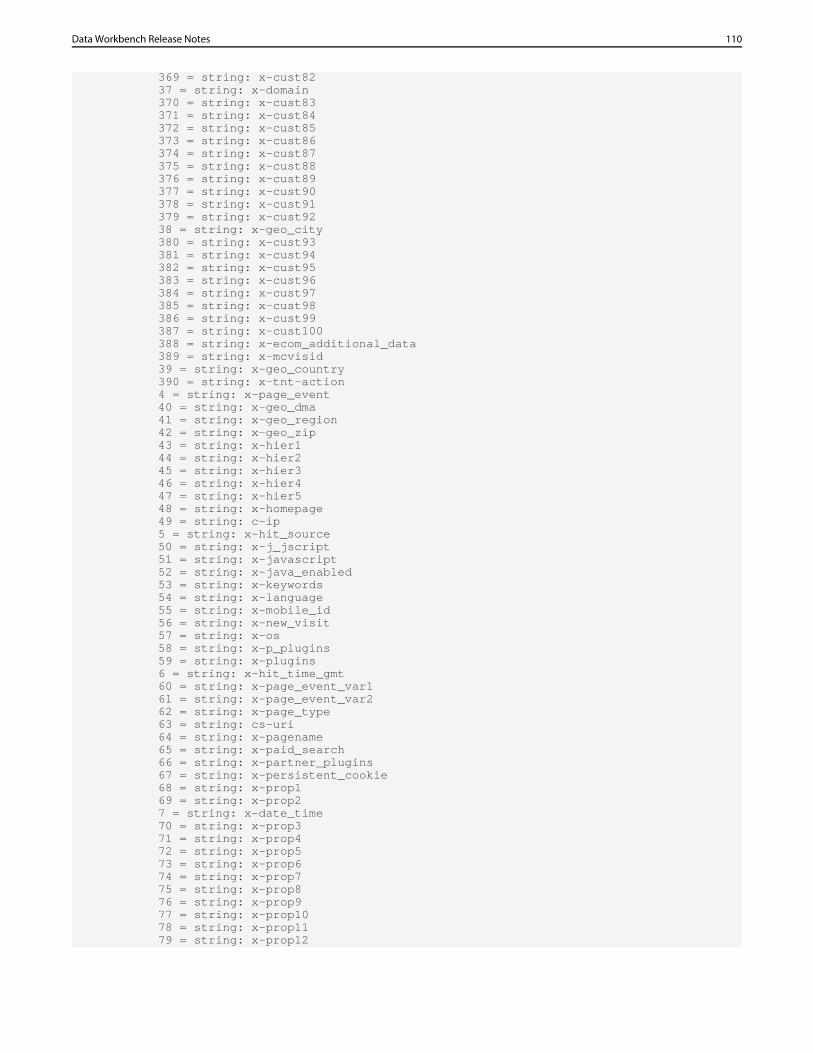
369 = string: x-cust82 37 = string: x-domain 370 = string: x-cust83 371 = string: x-cust84 372 = string: x-cust85 373 = string: x-cust86 374 = string: x-cust87 375 = string: x-cust88 376 = string: x-cust89 377 = string: x-cust90 378 = string: x-cust91 379 = string: x-cust92 38 = string: x-geo_city 380 = string: x-cust93 381 = string: x-cust94 382 = string: x-cust95 383 = string: x-cust96 384 = string: x-cust97 385 = string: x-cust98 386 = string: x-cust99 387 = string: x-cust100 388 = string: x-ecom_additional_data 389 = string: x-mcvisid 39 = string: x-geo_country 390 = string: x-tnt-action 4 = string: x-page_event 40 = string: x-geo_dma 41 = string: x-geo_region 42 = string: x-geo_zip 43 = string: x-hier1 44 = string: x-hier2 45 = string: x-hier3 46 = string: x-hier4 47 = string: x-hier5 48 = string: x-homepage 49 = string: c-ip 5 = string: x-hit_source 50 = string: x-j_jscript 51 = string: x-javascript 52 = string: x-java_enabled 53 = string: x-keywords 54 = string: x-language 55 = string: x-mobile_id 56 = string: x-new_visit 57 = string: x-os 58 = string: x-p_plugins 59 = string: x-plugins 6 = string: x-hit_time_gmt 60 = string: x-page_event_var1 61 = string: x-page_event_var2 62 = string: x-page_type 63 = string: cs-uri 64 = string: x-pagename 65 = string: x-paid_search 66 = string: x-partner_plugins 67 = string: x-persistent_cookie 68 = string: x-prop1 69 = string: x-prop2 7 = string: x-date_time 70 = string: x-prop3 71 = string: x-prop4 72 = string: x-prop5 73 = string: x-prop6 74 = string: x-prop7 75 = string: x-prop8 76 = string: x-prop9 77 = string: x-prop10 78 = string: x-prop11 79 = string: x-prop12
110Data Workbench Release Notes
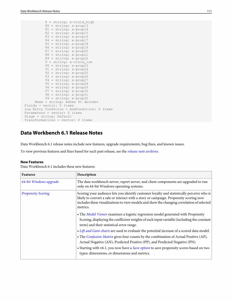
8 = string: x-visid_high 80 = string: x-prop13 81 = string: x-prop14 82 = string: x-prop15 83 = string: x-prop16 84 = string: x-prop17 85 = string: x-prop18 86 = string: x-prop19 87 = string: x-prop20 88 = string: x-prop21 89 = string: x-prop22 9 = string: x-visid_low 90 = string: x-prop23 91 = string: x-prop24 92 = string: x-prop25 93 = string: x-prop26 94 = string: x-prop27 95 = string: x-prop28 96 = string: x-prop29 97 = string: x-prop30 98 = string: x-prop31 99 = string: x-prop32 Name = string: Adobe SC decoder Fields = vector: 0 items Log Entry Condition = AndCondition: 0 items Parameters = vector: 0 items Stage = string: Default Transformations = vector: 0 items
Data Workbench 6.1 Release Notes
Data Workbench 6.1 release notes include new features, upgrade requirements, bug fixes, and known issues.
To view previous features and fixes based for each past release, see the release note archives.
New FeaturesData Workbench 6.1 includes these new features:
DescriptionFeatures
The data workbench server, report server, and client components are upgraded to runonly on 64-bit Windows operating systems.
64-bit Windows upgrade
Scoring your audience lets you identify customer loyalty and statistically perceive who islikely to convert a sale or interact with a story or campaign. Propensity scoring now
Propensity Scoring
includes these visualizations to view models and show the changing correlation of selectedmetrics.
• The Model Viewer examines a logistic regression model generated with PropensityScoring, displaying the coefficient weights of each input variable (including the constantterm) and their statistical error range.
• Lift and Gain charts are used to evaluate the potential increase of a scored data model.• The Confusion Matrix gives four counts by the combination of Actual Positive (AP),
Actual Negative (AN), Predicted Positive (PP), and Predicted Negative (PN).• Starting with v6.1, you now have a Save option to save propensity scores based on two
types: dimensions, or dimensions and metrics.
111Data Workbench Release Notes
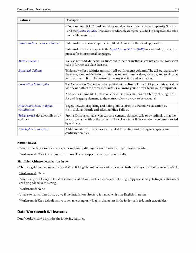
DescriptionFeatures
• You can now click Ctrl-Alt and drag and drop to add elements in Propensity Scoringand the Cluster Builder. Previously to add table elements, you had to drag from the tableto the Elements box.
Data workbench now supports Simplified Chinese for the client application.
Data workbench also supports the Input Method Editor (IME) as a secondary text entryprocess for international languages.
Data workbench now in Chinese
You can now add Mathematical functions to metrics, math transformations, and worksheetcells to further calculate datasets.
Math Functions
Tables now offer a statistics summary call-out for metric columns. The call-out can displaythe mean, standard deviation, minimum and maximum values, variance, and total countfor the column. It can be factored in to any selection and evaluation.
Statistical Callouts
The Correlation Matrix has been updated with a Binary Filter to let you constrain valuesfor one or both of the correlated metrics, allowing you to better focus your comparison.
Also, you can now add Dimension elements from a Dimension table by clicking Ctrl +Alt and dragging elements to the matrix column or row to be evaluated.
Correlation Matrix filter
Toggle between displaying and hiding fallout labels in a Funnel visualization byright-clicking the title and selecting Hide Fallout.
Hide Fallout label in funnelvisualization
From a Dimension table, you can sort elements alphabetically or by ordinals using thenew arrow in the title of the column. The # character will display when a column is sortedby ordinals.
Tables sorted alphabetically or byordinals
Additional shortcut keys have been added for adding and editing workspaces andconfiguration files.
New keyboard shortcuts
Known Issues
• When importing a workspace, an error message is displayed even though the import was successful.
Workaround: Click OK to ignore the error. The workspace is imported successfully.
Simplified Chinese Localization Issues
• The dialog title and message displayed after clicking "Submit" when setting the target in the Scoring visualization are unreadable.
Workaround: None.
• When using word wrap in the Worksheet visualization, localized words are not being wrapped correctly. Extra junk charactersare being added to the string.
Workaround: None
• Unable to launch Insight.exe if the installation directory is named with non-English characters.
Workaround: Keep default names or rename using only English characters in the folder path to launch executables.
Data Workbench 6.1 features
Data Workbench 6.1 includes the following features.
112Data Workbench Release Notes
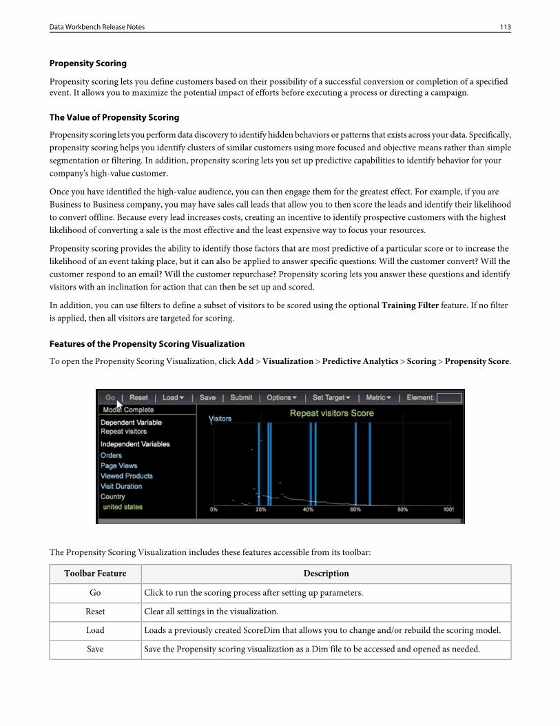
Propensity Scoring
Propensity scoring lets you define customers based on their possibility of a successful conversion or completion of a specifiedevent. It allows you to maximize the potential impact of efforts before executing a process or directing a campaign.
The Value of Propensity Scoring
Propensity scoring lets you perform data discovery to identify hidden behaviors or patterns that exists across your data. Specifically,propensity scoring helps you identify clusters of similar customers using more focused and objective means rather than simplesegmentation or filtering. In addition, propensity scoring lets you set up predictive capabilities to identify behavior for yourcompany's high-value customer.
Once you have identified the high-value audience, you can then engage them for the greatest effect. For example, if you areBusiness to Business company, you may have sales call leads that allow you to then score the leads and identify their likelihoodto convert offline. Because every lead increases costs, creating an incentive to identify prospective customers with the highestlikelihood of converting a sale is the most effective and the least expensive way to focus your resources.
Propensity scoring provides the ability to identify those factors that are most predictive of a particular score or to increase thelikelihood of an event taking place, but it can also be applied to answer specific questions: Will the customer convert? Will thecustomer respond to an email? Will the customer repurchase? Propensity scoring lets you answer these questions and identifyvisitors with an inclination for action that can then be set up and scored.
In addition, you can use filters to define a subset of visitors to be scored using the optional Training Filter feature. If no filteris applied, then all visitors are targeted for scoring.
Features of the Propensity Scoring Visualization
To open the Propensity Scoring Visualization, click Add > Visualization > Predictive Analytics > Scoring > Propensity Score.
The Propensity Scoring Visualization includes these features accessible from its toolbar:
DescriptionToolbar Feature
Click to run the scoring process after setting up parameters.Go
Clear all settings in the visualization.Reset
Loads a previously created ScoreDim that allows you to change and/or rebuild the scoring model.Load
Save the Propensity scoring visualization as a Dim file to be accessed and opened as needed.Save
113Data Workbench Release Notes
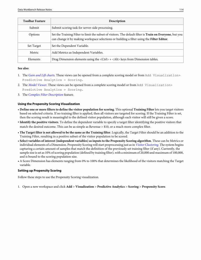
DescriptionToolbar Feature
Submit scoring task for server-side processing.Submit
Set the Training Filter to limit the subset of visitors. The default filter is Train on Everyone, but youcan change it by making workspace selections or building a filter using the Filter Editor.
Options
Set the Dependent Variable.Set Target
Add Metrics as Independent Variables.Metric
Drag Dimension elements using the <Ctrl> + <Alt> keys from Dimension tables.Elements
See also:
1. The Gain and Lift charts. These views can be opened from a complete scoring model or from Add Visualization>Predictive Analytics > Scoring.
2. The Model Viewer. These views can be opened from a complete scoring model or from Add Visualization>Predictive Analytics > Scoring.
3. The Complex Filter Description feature.
Using the Propensity Scoring Visualization
• Define one or more filters to define the visitor population for scoring. This optional Training Filter lets you target visitorsbased on selected criteria. If no training filter is applied, then all visitors are targeted for scoring. If the Training Filter is set,then the scoring result is meaningful to the defined visitor population, although each visitor will still be given a score.
• Identify the positive visitors. To define the dependent variable to specify a target filter identifying the positive visitors thatmatch the desired outcome. This can be as simple as Revenue > $10, or a much more complex filter.
• The Target filter is not allowed to be the same as the Training filter. Logically, the Target Filter should be an addition to theTraining Filter, resulting in a positive subset of the visitor population to be scored.
• Select variables of interest (independent variables) as inputs to the Propensity Scoring algorithm. These can be Metrics orindividual elements of a Dimension. Propensity Scoring will start preprocessing just as in Visitor Clustering. The system beginscapturing a certain amount of samples that match the definition of the previously set training filter (if any). Currently, thesample size is set as 10% of scoring population (defined by training filter), with a minimum of 20,000 and maximum of 100,000,and is bound to the scoring population size.
• A Score Dimension has elements ranging from 0% to 100% that determines the likelihood of the visitors matching the Targetvariable.
Setting up Propensity Scoring
Follow these steps to use the Propensity Scoring visualization.
1. Open a new workspace and click Add > Visualization > Predictive Analytics > Scoring > Propensity Score.
114Data Workbench Release Notes
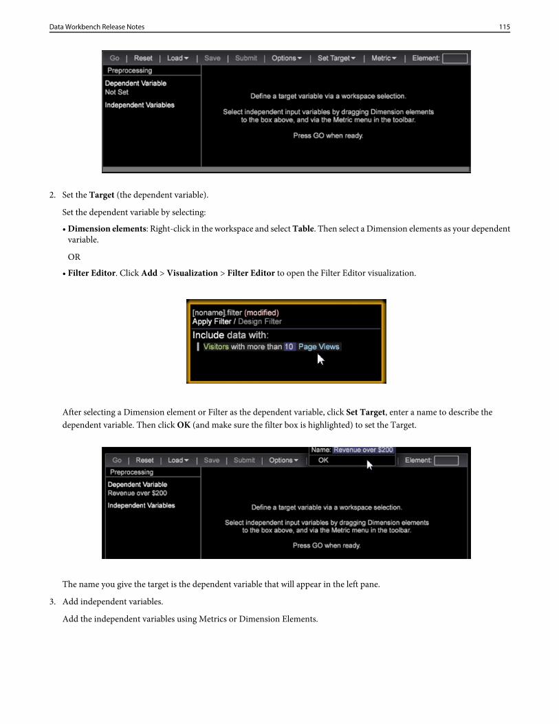
2. Set the Target (the dependent variable).
Set the dependent variable by selecting:
• Dimension elements: Right-click in the workspace and select Table. Then select a Dimension elements as your dependentvariable.
OR
• Filter Editor. Click Add > Visualization > Filter Editor to open the Filter Editor visualization.
After selecting a Dimension element or Filter as the dependent variable, click Set Target, enter a name to describe thedependent variable. Then click OK (and make sure the filter box is highlighted) to set the Target.
The name you give the target is the dependent variable that will appear in the left pane.
3. Add independent variables.
Add the independent variables using Metrics or Dimension Elements.
115Data Workbench Release Notes
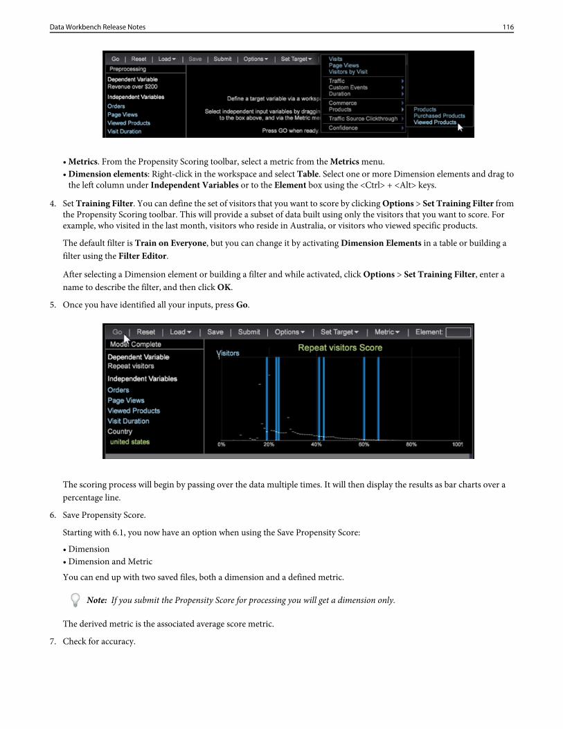
• Metrics. From the Propensity Scoring toolbar, select a metric from the Metrics menu.• Dimension elements: Right-click in the workspace and select Table. Select one or more Dimension elements and drag to
the left column under Independent Variables or to the Element box using the <Ctrl> + <Alt> keys.
4. Set Training Filter. You can define the set of visitors that you want to score by clicking Options > Set Training Filter fromthe Propensity Scoring toolbar. This will provide a subset of data built using only the visitors that you want to score. Forexample, who visited in the last month, visitors who reside in Australia, or visitors who viewed specific products.
The default filter is Train on Everyone, but you can change it by activating Dimension Elements in a table or building afilter using the Filter Editor.
After selecting a Dimension element or building a filter and while activated, click Options > Set Training Filter, enter aname to describe the filter, and then click OK.
5. Once you have identified all your inputs, press Go.
The scoring process will begin by passing over the data multiple times. It will then display the results as bar charts over apercentage line.
6. Save Propensity Score.
Starting with 6.1, you now have an option when using the Save Propensity Score:
• Dimension• Dimension and Metric
You can end up with two saved files, both a dimension and a defined metric.
Note: If you submit the Propensity Score for processing you will get a dimension only.
The derived metric is the associated average score metric.
7. Check for accuracy.
116Data Workbench Release Notes
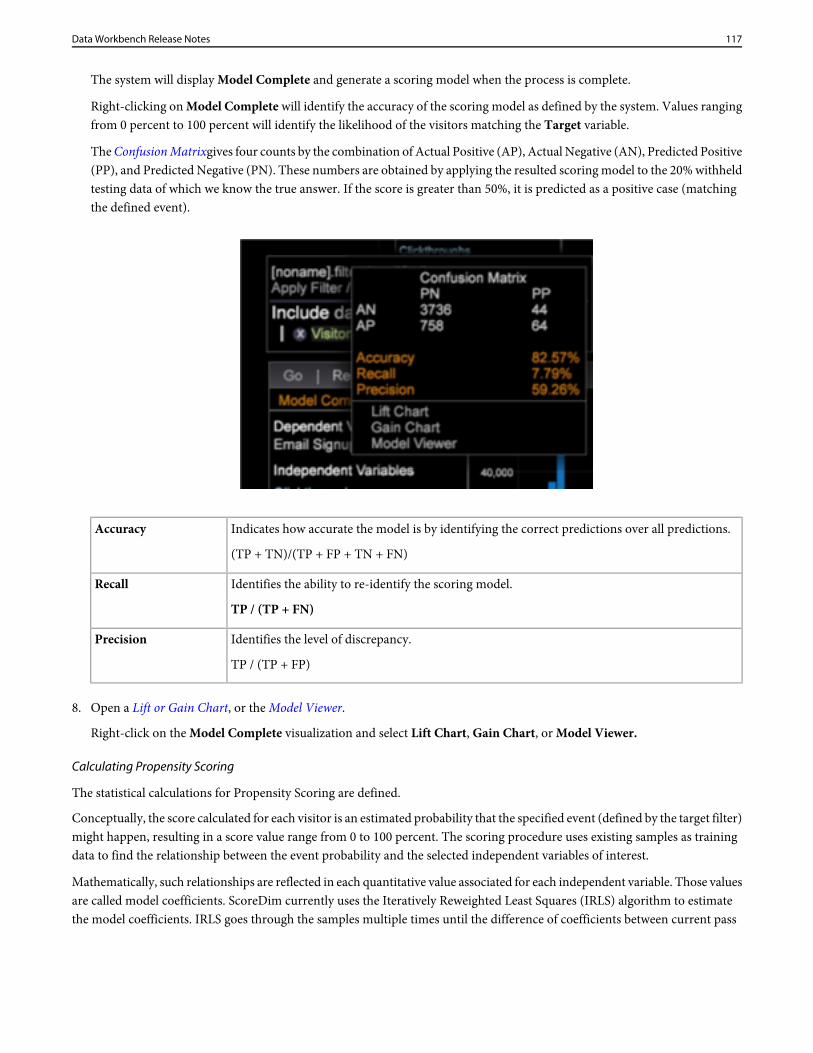
The system will display Model Complete and generate a scoring model when the process is complete.
Right-clicking on Model Complete will identify the accuracy of the scoring model as defined by the system. Values rangingfrom 0 percent to 100 percent will identify the likelihood of the visitors matching the Target variable.
The Confusion Matrixgives four counts by the combination of Actual Positive (AP), Actual Negative (AN), Predicted Positive(PP), and Predicted Negative (PN). These numbers are obtained by applying the resulted scoring model to the 20% withheldtesting data of which we know the true answer. If the score is greater than 50%, it is predicted as a positive case (matchingthe defined event).
Indicates how accurate the model is by identifying the correct predictions over all predictions.
(TP + TN)/(TP + FP + TN + FN)
Accuracy
Identifies the ability to re-identify the scoring model.
TP / (TP + FN)
Recall
Identifies the level of discrepancy.
TP / (TP + FP)
Precision
8. Open a Lift or Gain Chart, or the Model Viewer.
Right-click on the Model Complete visualization and select Lift Chart, Gain Chart, or Model Viewer.
Calculating Propensity Scoring
The statistical calculations for Propensity Scoring are defined.
Conceptually, the score calculated for each visitor is an estimated probability that the specified event (defined by the target filter)might happen, resulting in a score value range from 0 to 100 percent. The scoring procedure uses existing samples as trainingdata to find the relationship between the event probability and the selected independent variables of interest.
Mathematically, such relationships are reflected in each quantitative value associated for each independent variable. Those valuesare called model coefficients. ScoreDim currently uses the Iteratively Reweighted Least Squares (IRLS) algorithm to estimatethe model coefficients. IRLS goes through the samples multiple times until the difference of coefficients between current pass
117Data Workbench Release Notes
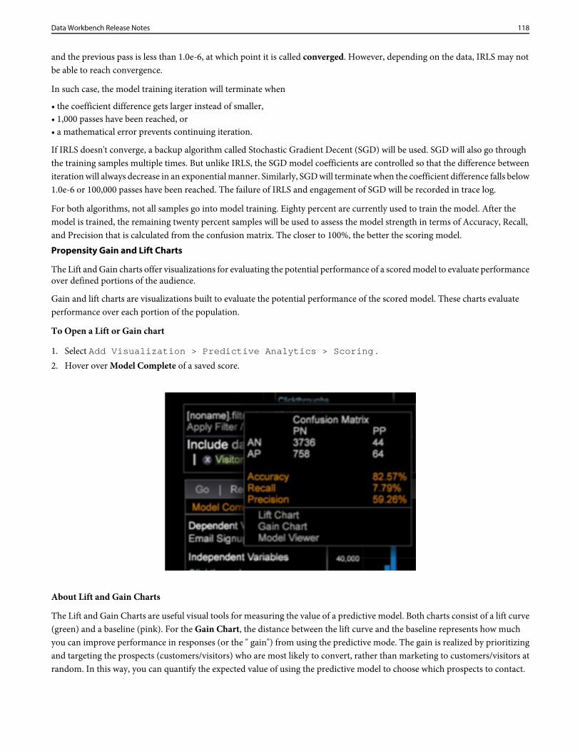
and the previous pass is less than 1.0e-6, at which point it is called converged. However, depending on the data, IRLS may notbe able to reach convergence.
In such case, the model training iteration will terminate when
• the coefficient difference gets larger instead of smaller,• 1,000 passes have been reached, or• a mathematical error prevents continuing iteration.
If IRLS doesn't converge, a backup algorithm called Stochastic Gradient Decent (SGD) will be used. SGD will also go throughthe training samples multiple times. But unlike IRLS, the SGD model coefficients are controlled so that the difference betweeniteration will always decrease in an exponential manner. Similarly, SGD will terminate when the coefficient difference falls below1.0e-6 or 100,000 passes have been reached. The failure of IRLS and engagement of SGD will be recorded in trace log.
For both algorithms, not all samples go into model training. Eighty percent are currently used to train the model. After themodel is trained, the remaining twenty percent samples will be used to assess the model strength in terms of Accuracy, Recall,and Precision that is calculated from the confusion matrix. The closer to 100%, the better the scoring model.Propensity Gain and Lift Charts
The Lift and Gain charts offer visualizations for evaluating the potential performance of a scored model to evaluate performanceover defined portions of the audience.
Gain and lift charts are visualizations built to evaluate the potential performance of the scored model. These charts evaluateperformance over each portion of the population.
To Open a Lift or Gain chart
1. Select Add Visualization > Predictive Analytics > Scoring .2. Hover over Model Complete of a saved score.
About Lift and Gain Charts
The Lift and Gain Charts are useful visual tools for measuring the value of a predictive model. Both charts consist of a lift curve(green) and a baseline (pink). For the Gain Chart, the distance between the lift curve and the baseline represents how muchyou can improve performance in responses (or the " gain") from using the predictive mode. The gain is realized by prioritizingand targeting the prospects (customers/visitors) who are most likely to convert, rather than marketing to customers/visitors atrandom. In this way, you can quantify the expected value of using the predictive model to choose which prospects to contact.
118Data Workbench Release Notes
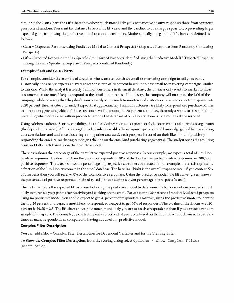
Similar to the Gain Chart, the Lift Chart shows how much more likely you are to receive positive responses than if you contactedprospects at random. You want the distance between the lift curve and the baseline to be as large as possible, representing largerexpected gains from using the predictive model to contact customers. Mathematically, the gain and lift charts are defined asfollows:
• Gain = (Expected Response using Predictive Model to Contact Prospects) / (Expected Response from Randomly ContactingProspects)
• Lift = (Expected Response among a Specific Group Size of Prospects identified using the Predictive Model) / (Expected Responseamong the same Specific Group Size of Prospects identified Randomly)
Example of Lift and Gain Charts
For example, consider the example of a retailer who wants to launch an email re-marketing campaign to sell yoga pants.Historically, the analyst expects an average response rate of 20 percent based upon past email re-marketing campaigns similarto this one. While the analyst has nearly 5 million customers in its email database, the business only wants to market to thosecustomers that are most likely to respond to the email and purchase. In this way, the company will maximize the ROI of thecampaign while ensuring that they don't unnecessarily send emails to uninterested customers. Given an expected response rateof 20 percent, the marketer and analyst expect that approximately 1 million customers are likely to respond and purchase. Ratherthan randomly guessing which of those customers will be among the 20 percent responses, the analyst wants to be smart aboutpredicting which of the one million prospects (among the database of 5 million customers) are most likely to respond.
Using Adobe's Audience Scoring capability, the analyst defines success as a prospect clicks on an email and purchases yoga pants(the dependent variable). After selecting the independent variables (based upon experience and knowledge gained from analyzingdata correlations and audience clustering among other analyses), each prospect is scored on their likelihood of positivelyresponding the email re-marketing campaign (clicking on the email and purchasing yoga pants). The analyst opens the resultingGain and Lift charts based upon the predictive model.
The y-axis shows the percentage of the cumulative expected positive responses. In our example, we expect a total of 1 millionpositive responses. A value of 20% on the y-axis corresponds to 20% of the 1 million expected positive responses, or 200,000positive responses. The x-axis shows the percentage of prospective customers contacted. In our example, the x-axis representsa fraction of the 5 million customers in the email database. The baseline (Pink) is the overall response rate - if you contact X%of prospects then you will receive X% of the total positive responses. Using the predictive model, the lift curve (green) showsthe percentage of positive responses obtained (y-axis) by contacting a given percentage of prospects (x-axis).
The Lift chart plots the expected lift as a result of using the predictive model to determine the top one million prospects mostlikely to purchase yoga pants after receiving and clicking on the email. For contacting 20 percent of randomly selected prospectsusing no predictive model, you should expect to get 20 percent of responders. However, using the predictive model to identifythe top 20 percent of prospects most likely to respond, you expect to get 50% of responders. The y-value of the lift curve at 20percent is 50/20 = 2.5. The lift chart shows how much more likely you are to receive respondents than if you contact a randomsample of prospects. For example, by contacting only 20 percent of prospects based on the predictive model you will reach 2.5times as many respondents as compared to having not used any predictive model.Complex Filter Description
You can add a Show Complex Filter Description for Dependent Variables and for the Training Filter.
To Show the Complex Filter Description, from the scoring dialog select Options > Show Complex FilterDescription.
119Data Workbench Release Notes
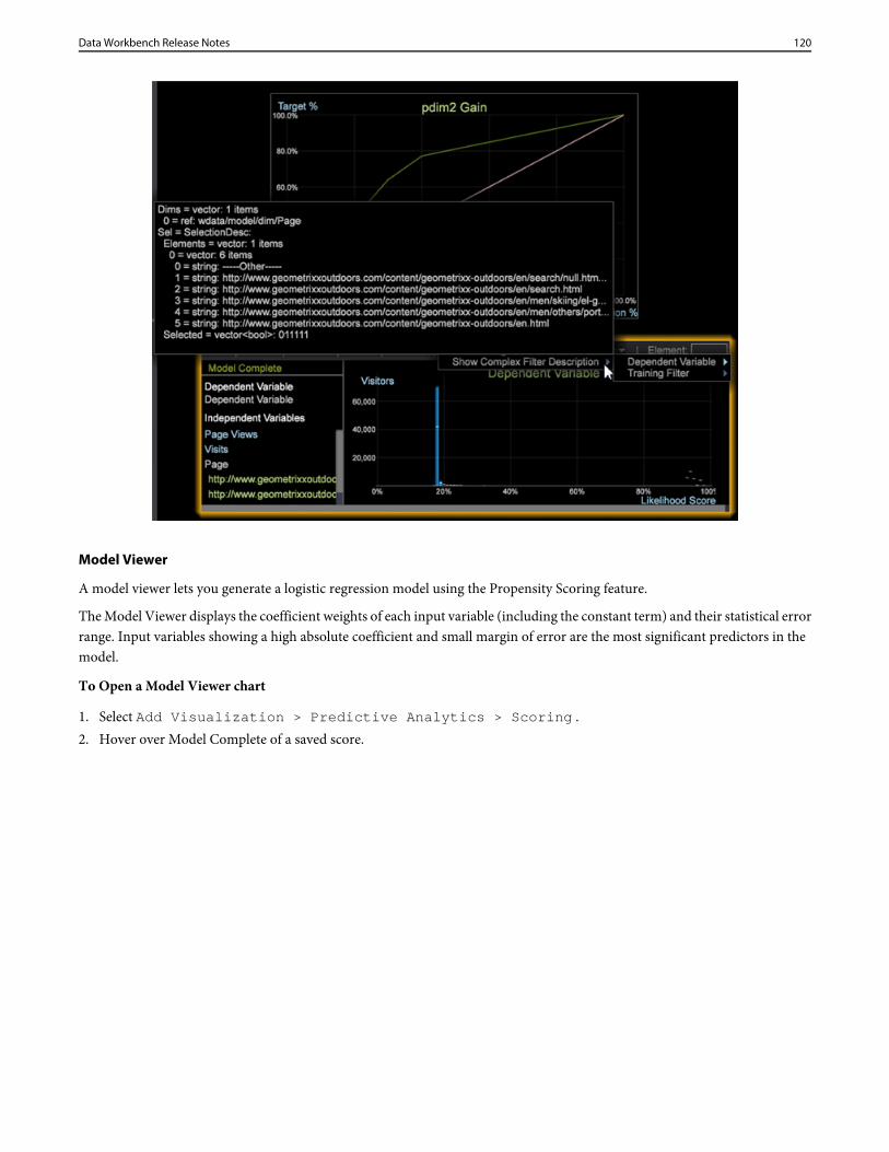
Model Viewer
A model viewer lets you generate a logistic regression model using the Propensity Scoring feature.
The Model Viewer displays the coefficient weights of each input variable (including the constant term) and their statistical errorrange. Input variables showing a high absolute coefficient and small margin of error are the most significant predictors in themodel.
To Open a Model Viewer chart
1. Select Add Visualization > Predictive Analytics > Scoring .2. Hover over Model Complete of a saved score.
120Data Workbench Release Notes
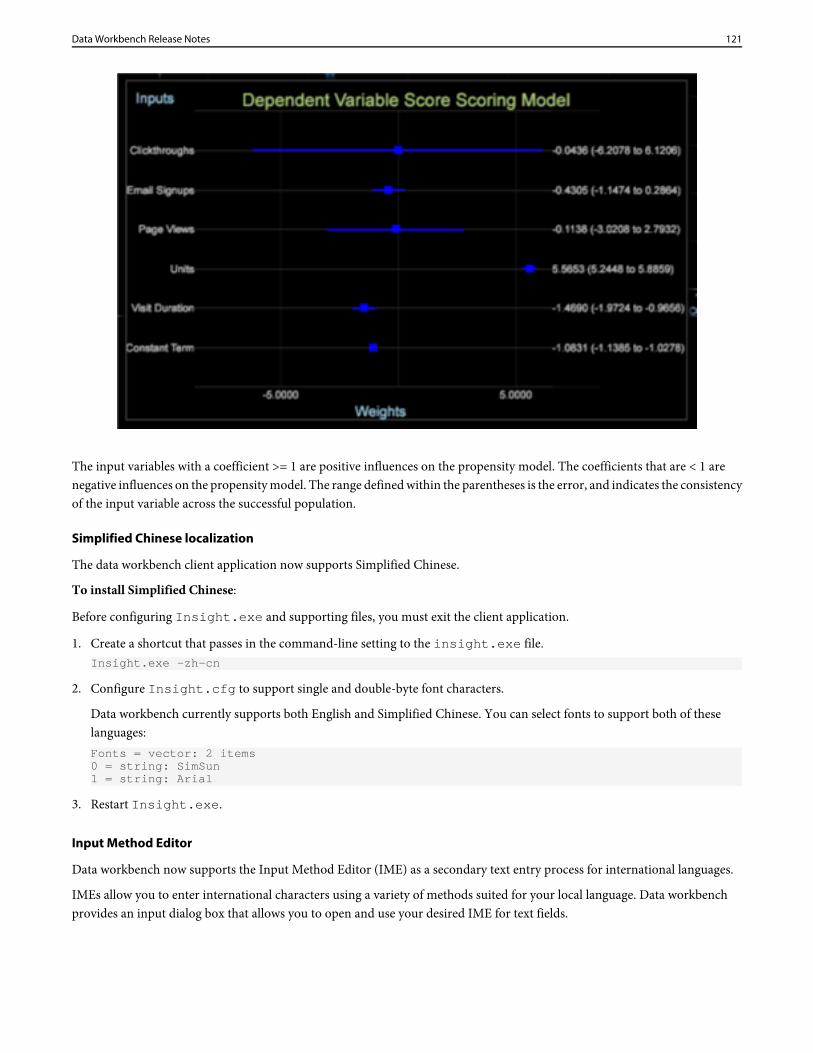
The input variables with a coefficient >= 1 are positive influences on the propensity model. The coefficients that are < 1 arenegative influences on the propensity model. The range defined within the parentheses is the error, and indicates the consistencyof the input variable across the successful population.
Simplified Chinese localization
The data workbench client application now supports Simplified Chinese.
To install Simplified Chinese:
Before configuring Insight.exe and supporting files, you must exit the client application.
1. Create a shortcut that passes in the command-line setting to the insight.exe file.Insight.exe -zh-cn
2. Configure Insight.cfg to support single and double-byte font characters.
Data workbench currently supports both English and Simplified Chinese. You can select fonts to support both of theselanguages:Fonts = vector: 2 items0 = string: SimSun1 = string: Arial
3. Restart Insight.exe.
Input Method Editor
Data workbench now supports the Input Method Editor (IME) as a secondary text entry process for international languages.
IMEs allow you to enter international characters using a variety of methods suited for your local language. Data workbenchprovides an input dialog box that allows you to open and use your desired IME for text fields.
121Data Workbench Release Notes
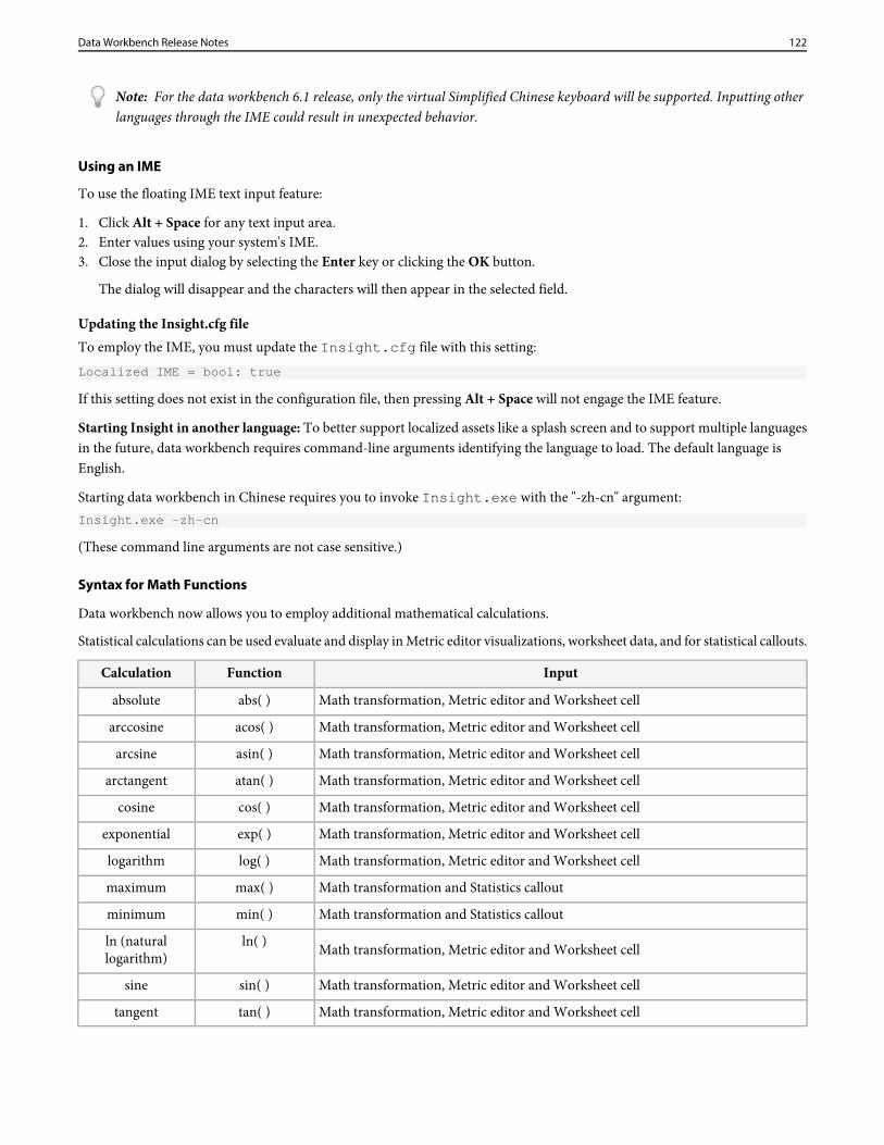
Note: For the data workbench 6.1 release, only the virtual Simplified Chinese keyboard will be supported. Inputting otherlanguages through the IME could result in unexpected behavior.
Using an IME
To use the floating IME text input feature:
1. Click Alt + Space for any text input area.2. Enter values using your system's IME.3. Close the input dialog by selecting the Enter key or clicking the OK button.
The dialog will disappear and the characters will then appear in the selected field.
Updating the Insight.cfg fileTo employ the IME, you must update the Insight.cfg file with this setting:Localized IME = bool: true
If this setting does not exist in the configuration file, then pressing Alt + Space will not engage the IME feature.
Starting Insight in another language: To better support localized assets like a splash screen and to support multiple languagesin the future, data workbench requires command-line arguments identifying the language to load. The default language isEnglish.
Starting data workbench in Chinese requires you to invoke Insight.exe with the "-zh-cn" argument:Insight.exe -zh-cn
(These command line arguments are not case sensitive.)
Syntax for Math Functions
Data workbench now allows you to employ additional mathematical calculations.
Statistical calculations can be used evaluate and display in Metric editor visualizations, worksheet data, and for statistical callouts.
InputFunctionCalculation
Math transformation, Metric editor and Worksheet cellabs( )absolute
Math transformation, Metric editor and Worksheet cellacos( )arccosine
Math transformation, Metric editor and Worksheet cellasin( )arcsine
Math transformation, Metric editor and Worksheet cellatan( )arctangent
Math transformation, Metric editor and Worksheet cellcos( )cosine
Math transformation, Metric editor and Worksheet cellexp( )exponential
Math transformation, Metric editor and Worksheet celllog( )logarithm
Math transformation and Statistics calloutmax( )maximum
Math transformation and Statistics calloutmin( )minimum
Math transformation, Metric editor and Worksheet cellln( )ln (naturallogarithm)
Math transformation, Metric editor and Worksheet cellsin( )sine
Math transformation, Metric editor and Worksheet celltan( )tangent
122Data Workbench Release Notes
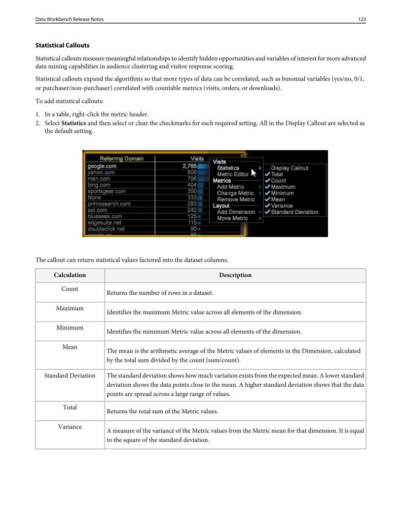
Statistical Callouts
Statistical callouts measure meaningful relationships to identify hidden opportunities and variables of interest for more advanceddata mining capabilities in audience clustering and visitor response scoring.
Statistical callouts expand the algorithms so that more types of data can be correlated, such as binomial variables (yes/no, 0/1,or purchaser/non-purchaser) correlated with countable metrics (visits, orders, or downloads).
To add statistical callouts:
1. In a table, right-click the metric header.2. Select Statistics and then select or clear the checkmarks for each required setting. All in the Display Callout are selected as
the default setting.
The callout can return statistical values factored into the dataset columns.
DescriptionCalculation
Returns the number of rows in a dataset.Count
Identifies the maximum Metric value across all elements of the dimension.Maximum
Identifies the minimum Metric value across all elements of the dimension.Minimum
The mean is the arithmetic average of the Metric values of elements in the Dimension, calculatedby the total sum divided by the count (sum/count).
Mean
The standard deviation shows how much variation exists from the expected mean. A lower standarddeviation shows the data points close to the mean. A higher standard deviation shows that the datapoints are spread across a large range of values.
Standard Deviation
Returns the total sum of the Metric values.Total
A measure of the variance of the Metric values from the Metric mean for that dimension. It is equalto the square of the standard deviation.
Variance
123Data Workbench Release Notes
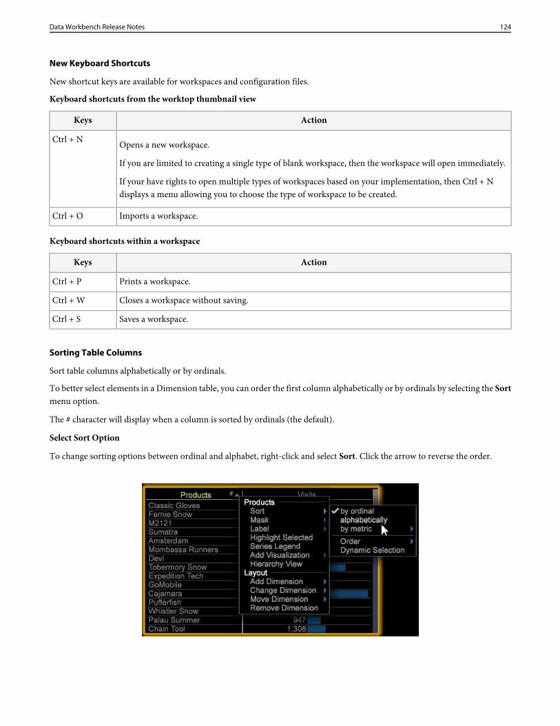
New Keyboard Shortcuts
New shortcut keys are available for workspaces and configuration files.
Keyboard shortcuts from the worktop thumbnail view
ActionKeys
Opens a new workspace.Ctrl + N
If you are limited to creating a single type of blank workspace, then the workspace will open immediately.
If your have rights to open multiple types of workspaces based on your implementation, then Ctrl + Ndisplays a menu allowing you to choose the type of workspace to be created.
Imports a workspace.Ctrl + O
Keyboard shortcuts within a workspace
ActionKeys
Prints a workspace.Ctrl + P
Closes a workspace without saving.Ctrl + W
Saves a workspace.Ctrl + S
Sorting Table Columns
Sort table columns alphabetically or by ordinals.
To better select elements in a Dimension table, you can order the first column alphabetically or by ordinals by selecting the Sortmenu option.
The # character will display when a column is sorted by ordinals (the default).
Select Sort Option
To change sorting options between ordinal and alphabet, right-click and select Sort. Click the arrow to reverse the order.
124Data Workbench Release Notes
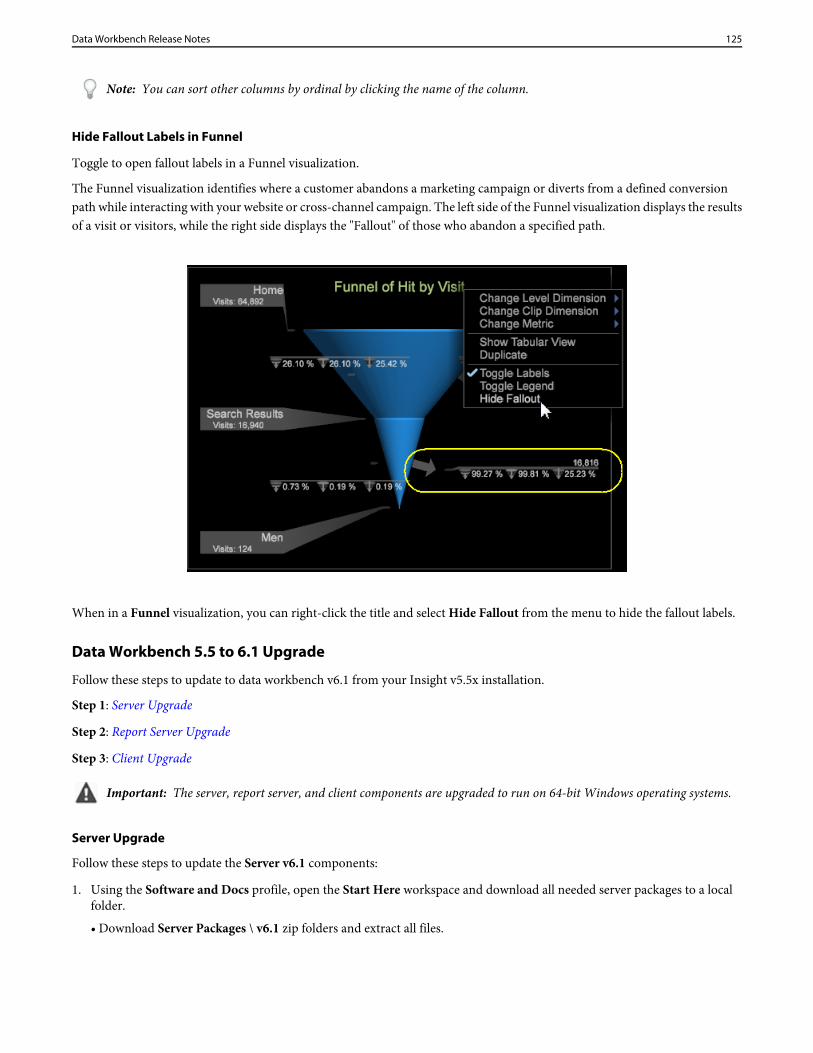
Note: You can sort other columns by ordinal by clicking the name of the column.
Hide Fallout Labels in Funnel
Toggle to open fallout labels in a Funnel visualization.
The Funnel visualization identifies where a customer abandons a marketing campaign or diverts from a defined conversionpath while interacting with your website or cross-channel campaign. The left side of the Funnel visualization displays the resultsof a visit or visitors, while the right side displays the "Fallout" of those who abandon a specified path.
When in a Funnel visualization, you can right-click the title and select Hide Fallout from the menu to hide the fallout labels.
Data Workbench 5.5 to 6.1 Upgrade
Follow these steps to update to data workbench v6.1 from your Insight v5.5x installation.
Step 1: Server Upgrade
Step 2: Report Server Upgrade
Step 3: Client Upgrade
Important: The server, report server, and client components are upgraded to run on 64-bit Windows operating systems.
Server Upgrade
Follow these steps to update the Server v6.1 components:
1. Using the Software and Docs profile, open the Start Here workspace and download all needed server packages to a localfolder.
• Download Server Packages \ v6.1 zip folders and extract all files.
125Data Workbench Release Notes
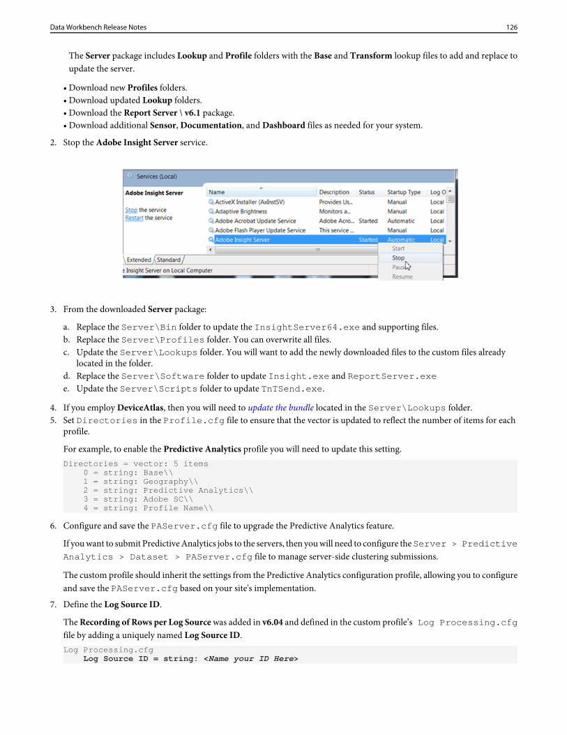
The Server package includes Lookup and Profile folders with the Base and Transform lookup files to add and replace toupdate the server.
• Download new Profiles folders.• Download updated Lookup folders.• Download the Report Server \ v6.1 package.• Download additional Sensor, Documentation, and Dashboard files as needed for your system.
2. Stop the Adobe Insight Server service.
3. From the downloaded Server package:
a. Replace the Server\Bin folder to update the InsightServer64.exe and supporting files.b. Replace the Server\Profiles folder. You can overwrite all files.c. Update the Server\Lookups folder. You will want to add the newly downloaded files to the custom files already
located in the folder.d. Replace the Server\Software folder to update Insight.exe and ReportServer.exee. Update the Server\Scripts folder to update TnTSend.exe.
4. If you employ DeviceAtlas, then you will need to update the bundle located in the Server\Lookups folder.5. Set Directories in the Profile.cfg file to ensure that the vector is updated to reflect the number of items for each
profile.
For example, to enable the Predictive Analytics profile you will need to update this setting.Directories = vector: 5 items 0 = string: Base\\ 1 = string: Geography\\ 2 = string: Predictive Analytics\\ 3 = string: Adobe SC\\ 4 = string: Profile Name\\
6. Configure and save the PAServer.cfg file to upgrade the Predictive Analytics feature.
If you want to submit Predictive Analytics jobs to the servers, then you will need to configure the Server > PredictiveAnalytics > Dataset > PAServer.cfg file to manage server-side clustering submissions.
The custom profile should inherit the settings from the Predictive Analytics configuration profile, allowing you to configureand save the PAServer.cfg based on your site's implementation.
7. Define the Log Source ID.
The Recording of Rows per Log Source was added in v6.04 and defined in the custom profile’s Log Processing.cfgfile by adding a uniquely named Log Source ID.Log Processing.cfg
Log Source ID = string: <Name your ID Here>
126Data Workbench Release Notes
If you do not have the Log Source ID defined, then you will get the following error:Missing Log Source ID in log processing.cfg. Log Source ID must be defined for all log sources.
8. Because the EventMessages.dll has been updated, it is required that you unregister and then register the Adobe InsightServer across the cluster.
• InsightServer64.exe /unregserver• InsightServer64.exe /regserver
9. Start the Adobe Insight Server service across the cluster.
The server installation is now complete.
Report Server Upgrade
Important: Before upgrading to Report Server v6.1, you must first upgrade to Server v6.1.
1. Using the Software and Docs profile, download v6.1 from the Report Server package to a local folder.2. Copy Report Server 6.1 from the downloaded package and replace the profile packages.
Note: The Insight.zbin file in the install folder is a backup file used for localization, and must be present inthe install directory. This file or other .zbin files will be used depending on the command-line settings passed whenstarting up.
3. (optional) Modify the report server configuration file to support double-byte characters.
Data workbench currently supports English (-en-us) and Chinese (–zh-cn). You need to set a font to support single anddouble-byte characters:Report Server.cfg - Add Fonts Fonts = vector: 2 items 0 = string: SimSun 1 = string: Arial
The Windows operating system must also have the listed fonts installed.
4. Configure Report Server v6.1.
a. Stop the Adobe Insight Report Server service.b. Launch a command prompt as an "Administrator".c. Navigate to the Report Server install folder.d. Delete the Report Server service using the following command:
ReportServer.exe /unregserver
5. Start the service based on the language settings:ReportServer.exe -RegServer -Locale -en-us (English)ReportServer.exe -RegServer -Locale –zh-cn (Simplified Chinese)
6. To verify that Report Server is running with the correct settings, open up Windows Service Manager and right-click AdobeInsight Report Server - Properties. The path to the executable will display the updated command-line settings.
The report server installation is now complete.
Client Upgrade
Important: Before upgrading to Client v6.1, the administrator must first upgrade to Server v6.1.
127Data Workbench Release Notes
1. Launch Insight.exe but DO NOT connect to any profiles.2. Edit the Insight.cfg file to not update software automatically.
Update Software = bool: false
3. Connect to Software and Docs profile (softdocs).4. Download Software\Insight Client\v6.10.5. (optional) Modify insight.cfg to support double-byte characters.
Data workbench currently supports both English and Simplified Chinese. Select fonts to support both of these languages:Fonts = vector: 2 items 0 = string: SimSun1 = string: Arial
6. Exit out of the client.7. Copy the files in the downloaded v6.1 client package to the Install folder.
Note: The Insight.zbin file in the install folder is a backup file used for localization, and must be present in theinstall directory. This file or other .zbin files will be used depending on the command-line settings passed when startingup.
For example, to launch Simplified Chinese, create a shortcut that passes in the command-line setting.Insight.exe -zh-cn
If you want to launch in English (default), then no command-line change is necessary.
8. Launch Insight.exe for English or the shortcut that you created for another language.9. Connect to your profile and allow the client to synchronize with the server.10. (optional) To employ the IME, make these changes to the Insight.cfg file:
Localized IME = bool: true
The Input Method Editor (IME) allows you to input international characters.
11. (optional) Edit the Insight.cfg file to automatically update software:Update Software = bool: true
See instructions for implementing the IME.12. Restart again after the profile synchronization to employ the most recent .zbin file.
The client installation is now complete.
Data Workbench 6.0 to 6.1 Upgrade
Follow these steps to update to data workbench v6.1 from your data workbench v6.0x installation.
Step 1: Server upgrade
Step 2: Report Server upgrade
Step 3: Client upgrade
Important: The server, report server, and client components are upgraded to run on 64-bit Windows operating systems.
Server Upgrade
Follow these steps to update the Server v6.1 components:
128Data Workbench Release Notes
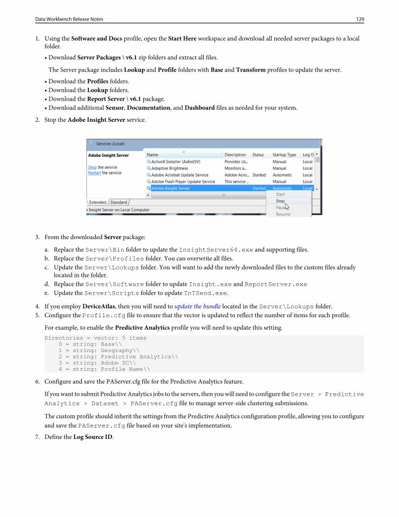
1. Using the Software and Docs profile, open the Start Here workspace and download all needed server packages to a localfolder.
• Download Server Packages \ v6.1 zip folders and extract all files.
The Server package includes Lookup and Profile folders with Base and Transform profiles to update the server.
• Download the Profiles folders.• Download the Lookup folders.• Download the Report Server \ v6.1 package.• Download additional Sensor, Documentation, and Dashboard files as needed for your system.
2. Stop the Adobe Insight Server service.
3. From the downloaded Server package:
a. Replace the Server\Bin folder to update the InsightServer64.exe and supporting files.b. Replace the Server\Profiles folder. You can overwrite all files.c. Update the Server\Lookups folder. You will want to add the newly downloaded files to the custom files already
located in the folder.d. Replace the Server\Software folder to update Insight.exe and ReportServer.exee. Update the Server\Scripts folder to update TnTSend.exe.
4. If you employ DeviceAtlas, then you will need to update the bundle located in the Server\Lookups folder.5. Configure the Profile.cfg file to ensure that the vector is updated to reflect the number of items for each profile.
For example, to enable the Predictive Analytics profile you will need to update this setting.Directories = vector: 5 items 0 = string: Base\\ 1 = string: Geography\\ 2 = string: Predictive Analytics\\ 3 = string: Adobe SC\\ 4 = string: Profile Name\\
6. Configure and save the PAServer.cfg file for the Predictive Analytics feature.
If you want to submit Predictive Analytics jobs to the servers, then you will need to configure the Server > PredictiveAnalytics > Dataset > PAServer.cfg file to manage server-side clustering submissions.
The custom profile should inherit the settings from the Predictive Analytics configuration profile, allowing you to configureand save the PAServer.cfg file based on your site's implementation.
7. Define the Log Source ID.
129Data Workbench Release Notes
The Recording of Rows per Log Source was added in v6.04 and defined in the custom profile’s Log Processing.cfgfile by adding a uniquely named Log Source ID.Log Processing.cfg
Log Source ID = string: <Name your ID Here>
If you do not have the Log Source ID defined, then you will get the following error:Missing Log Source ID in log processing.cfg. Log Source ID must be defined for all log sources.
8. Because the EventMessages.dll has been updated, it is required that you unregister and then register the Adobe InsightServer across the cluster.
• InsightServer64.exe /unregserver• InsightServer64.exe /regserver
9. Start the Adobe Insight Server service across the cluster.
The server installation is now complete.
Report Server Upgrade
Important: Before upgrading to Report Server v6.1, you must first upgrade to Server v6.1.
1. Using the Software and Docs profile, download v6.1 from the Report Server package to a local folder.2. Copy Report Server 6.1 from the downloaded package and replace the profile packages.
Note: The Insight.zbin file in the install folder is a backup file used for localization, and must be present inthe install directory. This file or other .zbin files will be used depending on the command-line settings passed whenstarting up.
3. (optional) Data workbench currently supports English (-en-us) and Chinese (–zh-cn). You need to set a font to supportsingle and double-byte characters:Report Server.cfg - Add Fonts Fonts = vector: 2 items 0 = string: SimSun 1 = string: Arial
The Windows operating system must also have the listed fonts installed.
4. Configure Report Server v6.1 for localization.
a. Stop the Adobe Insight Report Server service.b. Launch a command prompt as an "Administrator".c. Navigate to the Report Server install folder.d. Delete the Report Server service using the following command:
ReportServer.exe /unregserver
e. Start the service based on language settings:ReportServer.exe -RegServer -Locale -en-us (English) ReportServer.exe -RegServer -Locale –zh-cn (Simplified Chinese)
5. To verify that Report Server is running with the correct settings, open up Windows Service Manager and right-click AdobeInsight Report Server - Properties. The path to the executable will display the updated command-line settings.
The report server installation is now complete.
130Data Workbench Release Notes
Client Upgrade
Important: Before upgrading to Client v6.1, the administrator must first upgrade to Insight Server v6.1.
1. Launch Insight.exe but do not connect to any profiles.2. Edit the Insight.cfg file.
Update Software = bool: true
3. Connect to your profile.
Allow the client to synchronize with the server and your client will be upgraded with the latest v6.1client profiles, executables,and configuration files.
Note: The Insight.zbin file in the install folder is a backup file used for localization and must be present. Thisfile or other .zbin files will be used depending on the command-line settings passed when starting up.
See setting up localized languages to add an insight.zbin file required for localized settings.
Additional Client Settings
Before configuring Insight.exe and supporting files, you must exit the client application.
To install Simplified Chinese:
1. Create a shortcut that passes in the command-line setting to the Insight.exe file.Insight.exe -zh-cn
2. Configure Insight.cfg to support single and double-byte font characters.
Data workbench currently supports both English and Simplified Chinese. You can select fonts to support both of theselanguages:Fonts = vector: 2 items0 = string: SimSun1 = string: Arial
The Windows operating system must also have the requested fonts installed.
3. Launch the shortcut that you created to synchronize profiles and the updated .zbin file.
To employ the Input Method Editor (IME).
IME allows you to input international characters.
1. Update the Insight.cfg file with these settings:Localized IME = bool: true
2. Launch the shortcut that you created to synchronize profiles and the updated .zbin file.
The client installation is now complete.
Data Workbench 6.0 Release Notes
View the previous Data Workbench release notes.
See also the previous Insight release notes.
131Data Workbench Release Notes
Data Workbench 6.0 Release Notes
New features introduced in Data Workbench 6.0.4, including bug fixes and known issues.
New FeaturesData workbench (Insight 6.0) includes these new features and visualizations for added reporting capabilities and predictiveanalysis tools.
To view previous features and fixes based for each past release, see the release note archives.
DescriptionData Workbench Features
The Funnel visualization lets you define the sequential process flow of yourcustomers and provides visibility into the fallout of visitors at each step in theprocess.
Funnel Visualization
Clustering lets you leverage customer characteristics to dynamically categorizevisitors and generate cluster sets based on selected data inputs for customer analysisand targeting.
Visitor Clustering
Correlation Analysis lets you quickly identify relevant data relationships to extendand enhance your analysis.
Correlation Analysis
The DeviceAtlas JSON file will now be distributed in a .bundle file (a renamed.tar.gz) along with DeviceAtlas.dll and DeviceAtlas64.dll.
Updated DeviceAtlas Distribution
Client Upgrade Requirements
Complete these upgrade tasks for data workbench (Insight 6.0) client features:
Updating the .zbin file for the client
Data workbench now supports an Input Method Editor (IME) as a secondary text entry process that allows you to enterinternational characters from your keyboard using a floating text box. Data workbench will support English by default but alsoallows you to load other files to support international languages, such as a virtual Chinese keyboard (Pinyin IME).
A new dictionary file (a .zbin file) is required by the client application before updating to version 6.0. You can obtain the needed.zbin file from the Software and Docs profile (Softdocs).
Prerequisites:
• Before upgrading to the Insight 6.0 client and Report Server 6.0, the Insight administrator must first upgrade to Insight Server6.0.
• The Insight administrator will need to choose a zbin file based on language (en-us.zbin, zh-cn.zbin), copy the language file,then rename it to insight.zbin, and place the renamed file in the root directory of the Report Server where the executable islocated. Then restart the Insight Report Server.
See the Server Upgrade Requirements for additional server-side upgrade information.
To upgrade the zbin file for the client (from version 5.x to 6.0):
1. To make sure the client does not get updated from the Insight Server during this upgrade, set your Insight.cfg argument tofalse.Update Software = bool: false
2. Restart the Insight client.
132Data Workbench Release Notes
3. Navigate to the Software and Docs profile (SoftDocs profile) and download the required Insight.zbin file:Software\Insight Client\v6.00\Insight_6.00.zip
4. Copy the Insight.zbin file to the same folder as the Insight.exe file.5. To make sure the Insight client now gets updated from the Insight Server, change the Insight.cfg file argument to true:
Update Software = bool: true
6. Restart the client.
Your client will synchronize with the server and you will see a message stating that your client is downloading. At theconclusion of the download, you will get a message asking if your want to restart your Insight client.
7. Click OK to restart the client.
The client will start and upgrade to version 6.0.
8. Restart the client again for the Insight.zbin client synchronization to take effect.
If you get the following message, then it means the zbin was not placed in the correct folder location alongside the Insight.exefile.Insight Terminated: The backup dictionary file insight.zbinis missing.
To correct the issue, delete Insight.exe and rename the latest version of Insight.exe.old to Insight.exe, and then start againwith Step 1 above.
Server Upgrade Requirements
Complete these upgrade tasks for Insight 6.0 server features:
Update all Insight Server 6.0 packages. Insight 6.0 includes server packages that need to be updated, including the new PredictiveAnalytics profile.
•Important: It is recommended that users upgrade their server clusters with fresh installations of Insight Server 6.0 whenupdating.
It is also recommended that client upgrade their server clusters with fresh installation of Insight Server 6.0.
Upgrade Server cluster
Prepare the language file (.zbin file). The Insight administrator selects the <language>.zbin file for the required language (forexample: en-us.zbin , zh-cn.zbin) located in the base/localization/<langauge>.zbin folder. The administratorthen copies the language file and renames it to "insight.zbin".
After preparing the language file (.zbin), both the Insight Client and Report Server need to be updated. The Insight Client isupdated during the client upgrade process, but in most cases the Insight administrator will update the Report Server.
Update Report Server with a language file (.zbin file).
For all languages, Report Server 6.0 requires the "insight.zbin" file copied to the Report Server root folder.
Update the Report Server language files:
1. Add the renamed "insight.zbin" file to the root ReportServer directory.2. The Report Server configuration file (reportserver.cfg) requires font settings for double-byte languages. For example, Chinese
requires the addition of fonts using SimSun:Report Server.cfg - Add Fonts
Fonts = vector: 2 items
133Data Workbench Release Notes
0 = string: SimSun 1 = string: Arial
3. A parameter for Report Server 6.0 needs to be passed in the command line for localization, for example:ReportServer.exe -Locale -zh-cnReportServer.exe -Locale -en-us
Note: If a locale is not specified, then the Report Server defaults to the language selected in the insight.zbin file.
Follow the steps to launch the ReportServer as a service with the Locale parameters:
a. Launch a Command Prompt as an Administrator.b. Navigate to the ReportServer install folder.c. Type the following command to start the service:
• For English: ReportServer.exe -RegServer -Locale -en-us• For Chinese: ReportServer.exe -RegServer -Locale -zh-cn
4. To verify if the ReportServer is running with the correct parameters:
a. Open up Windows Service Manager.b. Right-click Adobe Insight Report Server - Properties.
The path to executable will contain the parameters:
ReportServer.exe -Service ReportServer -Locale -en-us
Modify Profile Configuration file for Predictive Analytics. Insight administrator will need to modify the custom profile.cfgfile to include the Predictive Analytics profile to be available in Insight.
Example of the profile.cfg entry:Example ("profile.cfg"):Profile = profileInfo: Active = bool: true Directories = vector: 5 items 0 = string: Base\\ 1 = string: Predictive Analytics\\ 2 = string: Geography\\ 3 = string: Adobe SC\\ 4 = string: Custom Profile\\
Update the PAServer.cfg file. If you want to submit Predictive Analytics clustering jobs to Insight Servers, then you will needto configure the PAServer.cfg file for handling server-side clustering submissions.
The custom profile should inherit the PAServer.cfg from the Predictive Analytics profile (Server\Profiles\PredictiveAnalytics\Dataset). Configure and save the PAServer.cfg per your implementation site.
Note: Once PAServer.cfg is configured and saved to custom profile, an Insight Server restart is required across the site.
Upgrade Report Server. You will need to update the fonts and the start-up parameters for Report Server.
Prerequisites:
• Before upgrading Report Server 6.0, the Insight administrator must first upgrade to Insight Server 6.0.• For all languages, Report Server 6.0 requires the addition of Insight.zbin to the Report Server root folder. Make sure the
base/localization/<langauge>.zbin is copied and renamed to "insight.zbin". Copy it to the root of the Report Server directory.
Update the Fonts and Start-up parameters:
134Data Workbench Release Notes

1. Report Server requires font setting for double byte in order to output to different languages,
for example:
Report Server.cfg - Add FontsFonts = vector: 2 items0 = string: SimSun1 = string: Arial
2. Parameter for Report Server 6.0 needs to be passed in the command-line for localization purposes.
To launch the Report Server as a service with the Locale parameters:
1. Stop the Report Server Service.2. Launch a Command Prompt as an Administrator.3. Navigate to the Report Server install folder.4. Type the following command to start the service:
ReportServer.exe -RegServer -Locale -en-us
To verify if the Report Server is running with the correct parameters:
1. Open up Windows Service Manager
2. Right-click Adobe Insight Report Server - Properties.3. The path to executable will contain the parameters:
ReportServer.exe -Service ReportServer -Locale -en-us
Upgrade the SiteCatalyst data feed for Insight 6.0. The filename format of the SiteCatalyst data feed for Insight 6.0 has changed.
Current filename format:
RSID_YYYYMMDD_HH0000.tsv.gz
New filename format:YYYYMMDD-RSID_HH0000.tsv.gz
Note: This change does not affect users currently deployed with the wbench/ecom version of the SiteCatalyst data feed.
The filename format change will allow for the full use of the Insight Start and End time declarations during log processing. Thisenables the process to evaluate if the contents of the file should be read, rather than filter all source files using a row by rowsearch.
In most cases, a rename process was implemented upon receipt of the file to provide the full use of this capability. This modificationprovides the required naming convention by default without the need and overhead of a secondary process.
To use the new SiteCatalyst data feed:
1. Determine how the receiving process will handle the new filename format.
The standard rename/move scripts deployed during implementation moves the files with a ".gz" extension, and only performsa rename if the filename matched the filename format with the preceding RSID.
The new filename format: YYYYMMDD-RSID_HH0000.tsv.gz
2. Evaluate the defined log source paths to confirm that all files will be read.
135Data Workbench Release Notes
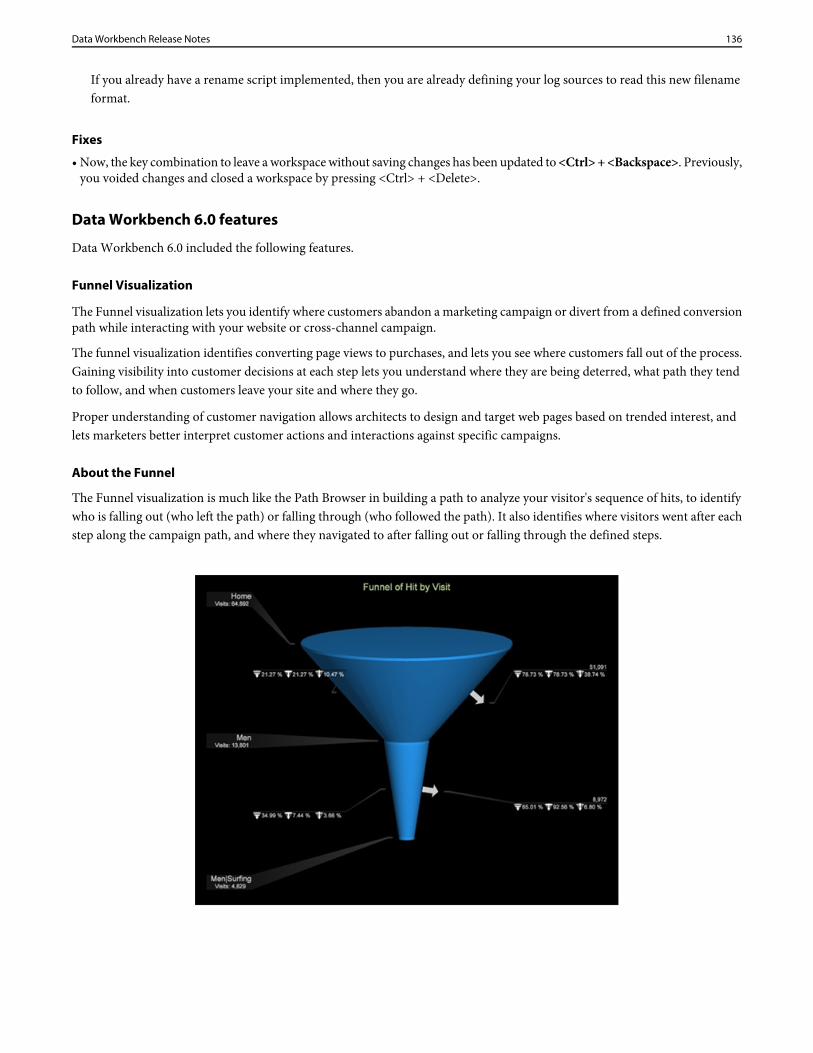
If you already have a rename script implemented, then you are already defining your log sources to read this new filenameformat.
Fixes
• Now, the key combination to leave a workspace without saving changes has been updated to <Ctrl> + <Backspace>. Previously,you voided changes and closed a workspace by pressing <Ctrl> + <Delete>.
Data Workbench 6.0 features
Data Workbench 6.0 included the following features.
Funnel Visualization
The Funnel visualization lets you identify where customers abandon a marketing campaign or divert from a defined conversionpath while interacting with your website or cross-channel campaign.
The funnel visualization identifies converting page views to purchases, and lets you see where customers fall out of the process.Gaining visibility into customer decisions at each step lets you understand where they are being deterred, what path they tendto follow, and when customers leave your site and where they go.
Proper understanding of customer navigation allows architects to design and target web pages based on trended interest, andlets marketers better interpret customer actions and interactions against specific campaigns.
About the Funnel
The Funnel visualization is much like the Path Browser in building a path to analyze your visitor's sequence of hits, to identifywho is falling out (who left the path) or falling through (who followed the path). It also identifies where visitors went after eachstep along the campaign path, and where they navigated to after falling out or falling through the defined steps.
136Data Workbench Release Notes
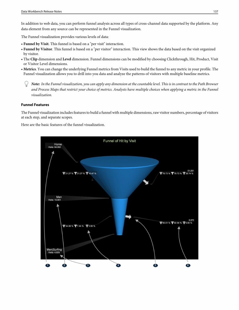
In addition to web data, you can perform funnel analysis across all types of cross-channel data supported by the platform. Anydata element from any source can be represented in the Funnel visualization.
The Funnel visualization provides various levels of data:
• Funnel by Visit. This funnel is based on a "per visit" interaction.• Funnel by Visitor. This funnel is based on a "per visitor" interaction. This view shows the data based on the visit organized
by visitor.• The Clip dimension and Level dimension. Funnel dimensions can be modified by choosing Clickthrough, Hit, Product, Visit
or Visitor Level dimensions.• Metrics. You can change the underlying Funnel metrics from Visits used to build the funnel to any metric in your profile. The
Funnel visualization allows you to drill into you data and analyze the patterns of visitors with multiple baseline metrics.
Note: In the Funnel visualization, you can apply any dimension at the countable level. This is in contrast to the Path Browserand Process Maps that restrict your choice of metrics. Analysts have multiple choices when applying a metric in the Funnelvisualization.
Funnel Features
The Funnel visualization includes features to build a funnel with multiple dimensions, raw visitor numbers, percentage of visitorsat each step, and separate scopes.
Here are the basic features of the funnel visualization.
137Data Workbench Release Notes
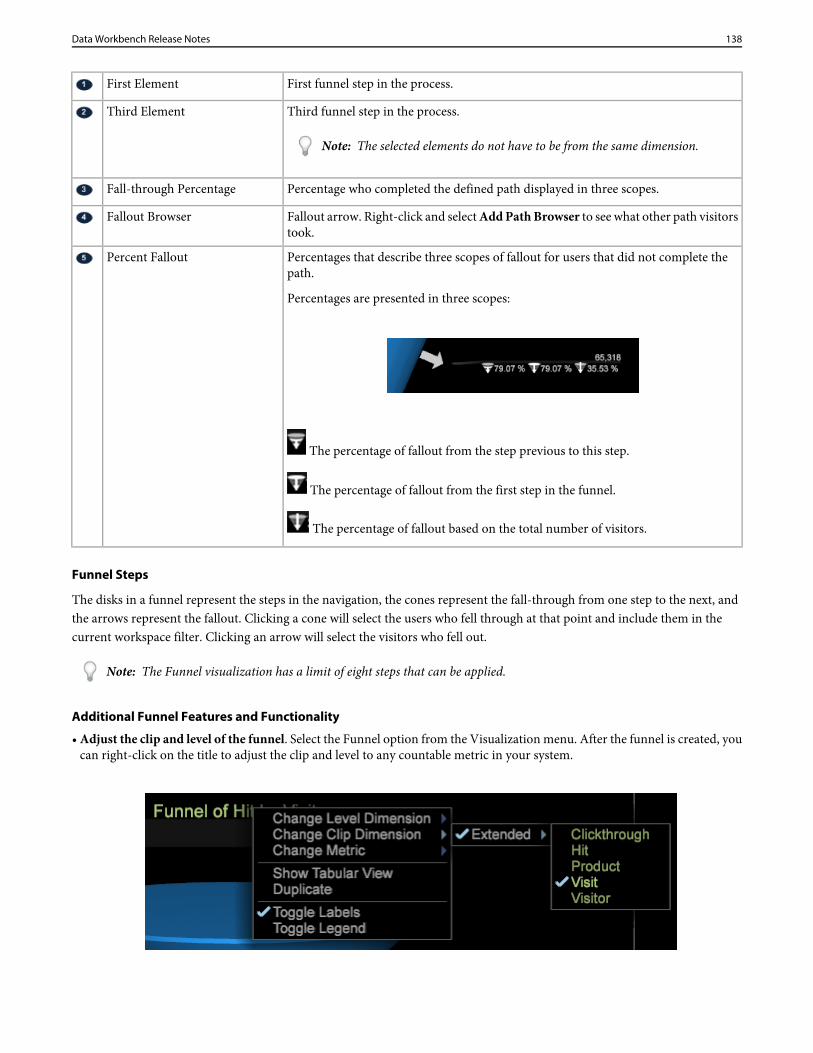
First funnel step in the process.First Element
Third funnel step in the process.Third Element
Note: The selected elements do not have to be from the same dimension.
Percentage who completed the defined path displayed in three scopes.Fall-through Percentage
Fallout arrow. Right-click and select Add Path Browser to see what other path visitorstook.
Fallout Browser
Percentages that describe three scopes of fallout for users that did not complete thepath.
Percentages are presented in three scopes:
Percent Fallout
The percentage of fallout from the step previous to this step.
The percentage of fallout from the first step in the funnel.
The percentage of fallout based on the total number of visitors.
Funnel Steps
The disks in a funnel represent the steps in the navigation, the cones represent the fall-through from one step to the next, andthe arrows represent the fallout. Clicking a cone will select the users who fell through at that point and include them in thecurrent workspace filter. Clicking an arrow will select the visitors who fell out.
Note: The Funnel visualization has a limit of eight steps that can be applied.
Additional Funnel Features and Functionality
• Adjust the clip and level of the funnel. Select the Funnel option from the Visualization menu. After the funnel is created, youcan right-click on the title to adjust the clip and level to any countable metric in your system.
138Data Workbench Release Notes
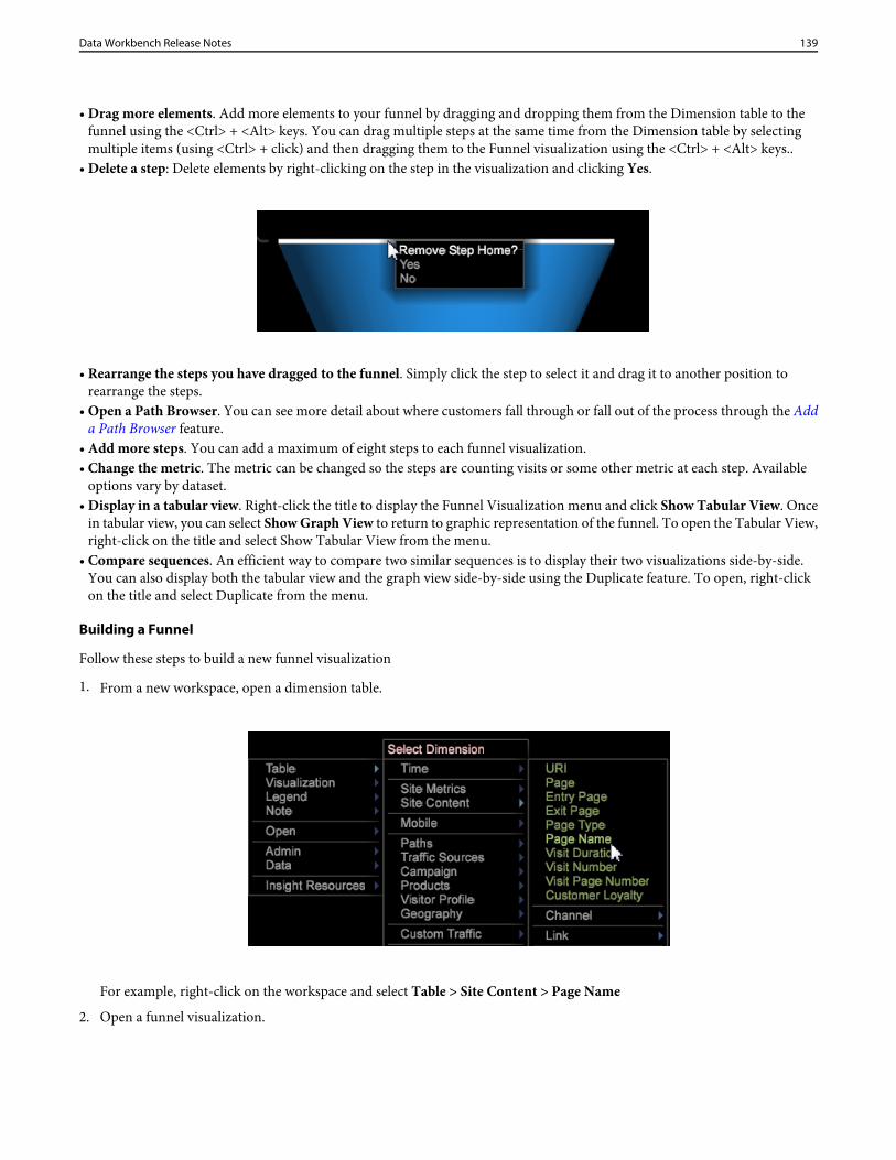
• Drag more elements. Add more elements to your funnel by dragging and dropping them from the Dimension table to thefunnel using the <Ctrl> + <Alt> keys. You can drag multiple steps at the same time from the Dimension table by selectingmultiple items (using <Ctrl> + click) and then dragging them to the Funnel visualization using the <Ctrl> + <Alt> keys..
• Delete a step: Delete elements by right-clicking on the step in the visualization and clicking Yes.
• Rearrange the steps you have dragged to the funnel. Simply click the step to select it and drag it to another position torearrange the steps.
• Open a Path Browser. You can see more detail about where customers fall through or fall out of the process through the Adda Path Browser feature.
• Add more steps. You can add a maximum of eight steps to each funnel visualization.• Change the metric. The metric can be changed so the steps are counting visits or some other metric at each step. Available
options vary by dataset.• Display in a tabular view. Right-click the title to display the Funnel Visualization menu and click Show Tabular View. Once
in tabular view, you can select Show Graph View to return to graphic representation of the funnel. To open the Tabular View,right-click on the title and select Show Tabular View from the menu.
• Compare sequences. An efficient way to compare two similar sequences is to display their two visualizations side-by-side.You can also display both the tabular view and the graph view side-by-side using the Duplicate feature. To open, right-clickon the title and select Duplicate from the menu.
Building a Funnel
Follow these steps to build a new funnel visualization
1. From a new workspace, open a dimension table.
For example, right-click on the workspace and select Table > Site Content > Page Name
2. Open a funnel visualization.
139Data Workbench Release Notes
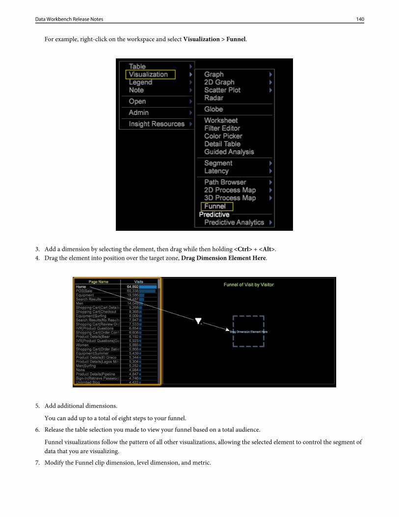
For example, right-click on the workspace and select Visualization > Funnel.
3. Add a dimension by selecting the element, then drag while then holding <Ctrl> + <Alt>.4. Drag the element into position over the target zone, Drag Dimension Element Here.
5. Add additional dimensions.
You can add up to a total of eight steps to your funnel.
6. Release the table selection you made to view your funnel based on a total audience.
Funnel visualizations follow the pattern of all other visualizations, allowing the selected element to control the segment ofdata that you are visualizing.
7. Modify the Funnel clip dimension, level dimension, and metric.
140Data Workbench Release Notes
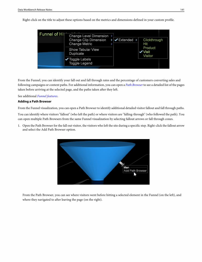
Right-click on the title to adjust these options based on the metrics and dimensions defined in your custom profile.
From the Funnel, you can identify your fall out and fall through rates and the percentage of customers converting sales andfollowing campaigns or content paths. For additional information, you can open a Path Browser to see a detailed list of the pagestaken before arriving at the selected page, and the paths taken after they left.
See additional Funnel features.Adding a Path Browser
From the Funnel visualization, you can open a Path Browser to identify additional detailed visitor fallout and fall through paths.
You can identify where visitors "fallout" (who left the path) or where visitors are "falling-through" (who followed the path). Youcan open multiple Path Browsers from the same Funnel visualization by selecting fallout arrows or fall through cones.
1. Open the Path Browser for the fall out visitor, the visitors who left the site during a specific step. Right-click the fallout arrowand select the Add Path Browser option.
From the Path Browser, you can see where visitors went before hitting a selected element in the Funnel (on the left), andwhere they navigated to after leaving the page (on the right).
141Data Workbench Release Notes
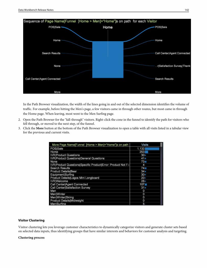
In the Path Browser visualization, the width of the lines going in and out of the selected dimension identifies the volume oftraffic. For example, before hitting the Men's page, a few visitors came in through other routes, but most came in throughthe Home page. When leaving, most went to the Men Surfing page.
2. Open the Path Browser for the "fall-through" visitors. Right-click the cone in the funnel to identify the path for visitors whofell through, or moved to the next step, of the funnel.
3. Click the More button at the bottom of the Path Browser visualization to open a table with all visits listed in a tabular viewfor the previous and current visits.
Visitor Clustering
Visitor clustering lets you leverage customer characteristics to dynamically categorize visitors and generate cluster sets basedon selected data inputs, thus identifying groups that have similar interests and behaviors for customer analysis and targeting.
Clustering process
142Data Workbench Release Notes
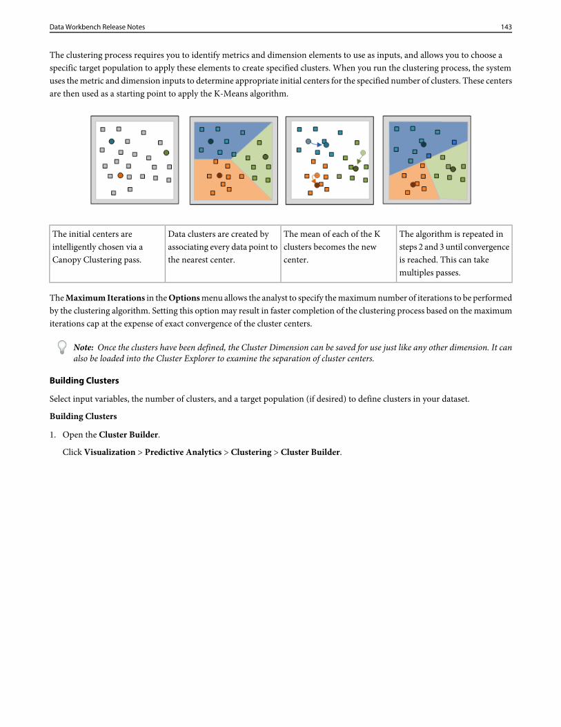
The clustering process requires you to identify metrics and dimension elements to use as inputs, and allows you to choose aspecific target population to apply these elements to create specified clusters. When you run the clustering process, the systemuses the metric and dimension inputs to determine appropriate initial centers for the specified number of clusters. These centersare then used as a starting point to apply the K-Means algorithm.
The algorithm is repeated insteps 2 and 3 until convergence
The mean of each of the Kclusters becomes the newcenter.
Data clusters are created byassociating every data point tothe nearest center.
The initial centers areintelligently chosen via aCanopy Clustering pass. is reached. This can take
multiples passes.
The Maximum Iterations in the Options menu allows the analyst to specify the maximum number of iterations to be performedby the clustering algorithm. Setting this option may result in faster completion of the clustering process based on the maximumiterations cap at the expense of exact convergence of the cluster centers.
Note: Once the clusters have been defined, the Cluster Dimension can be saved for use just like any other dimension. It canalso be loaded into the Cluster Explorer to examine the separation of cluster centers.
Building Clusters
Select input variables, the number of clusters, and a target population (if desired) to define clusters in your dataset.
Building Clusters
1. Open the Cluster Builder.
Click Visualization > Predictive Analytics > Clustering > Cluster Builder.
143Data Workbench Release Notes
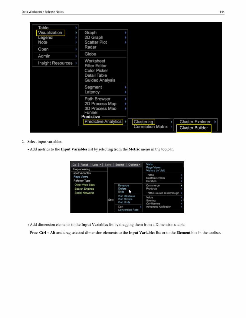
2. Select input variables.
• Add metrics to the Input Variables list by selecting from the Metric menu in the toolbar.
• Add dimension elements to the Input Variables list by dragging them from a Dimension's table.
Press Ctrl + Alt and drag selected dimension elements to the Input Variables list or to the Element box in the toolbar.
144Data Workbench Release Notes
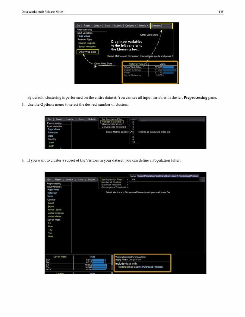
By default, clustering is performed on the entire dataset. You can see all input variables in the left Preprocessing pane.
3. Use the Options menu to select the desired number of clusters.
4. If you want to cluster a subset of the Visitors in your dataset, you can define a Population Filter.
145Data Workbench Release Notes
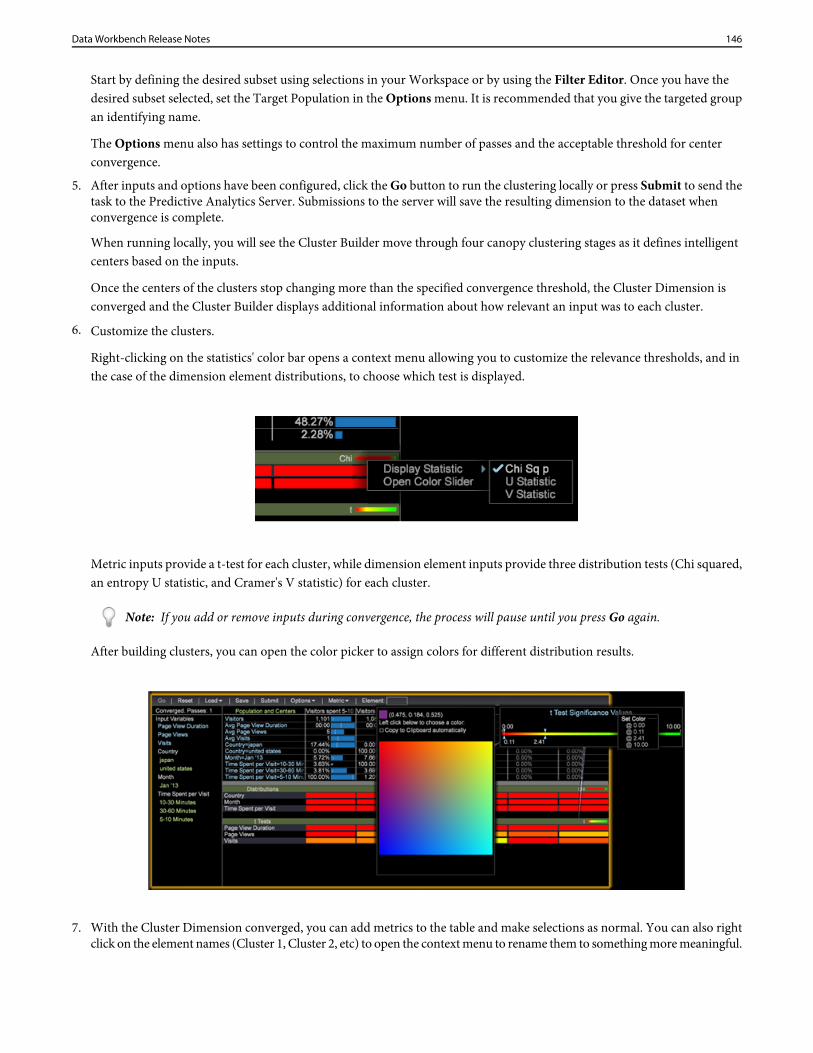
Start by defining the desired subset using selections in your Workspace or by using the Filter Editor. Once you have thedesired subset selected, set the Target Population in the Options menu. It is recommended that you give the targeted groupan identifying name.
The Options menu also has settings to control the maximum number of passes and the acceptable threshold for centerconvergence.
5. After inputs and options have been configured, click the Go button to run the clustering locally or press Submit to send thetask to the Predictive Analytics Server. Submissions to the server will save the resulting dimension to the dataset whenconvergence is complete.
When running locally, you will see the Cluster Builder move through four canopy clustering stages as it defines intelligentcenters based on the inputs.
Once the centers of the clusters stop changing more than the specified convergence threshold, the Cluster Dimension isconverged and the Cluster Builder displays additional information about how relevant an input was to each cluster.
6. Customize the clusters.
Right-clicking on the statistics' color bar opens a context menu allowing you to customize the relevance thresholds, and inthe case of the dimension element distributions, to choose which test is displayed.
Metric inputs provide a t-test for each cluster, while dimension element inputs provide three distribution tests (Chi squared,an entropy U statistic, and Cramer's V statistic) for each cluster.
Note: If you add or remove inputs during convergence, the process will pause until you press Go again.
After building clusters, you can open the color picker to assign colors for different distribution results.
7. With the Cluster Dimension converged, you can add metrics to the table and make selections as normal. You can also rightclick on the element names (Cluster 1, Cluster 2, etc) to open the context menu to rename them to something more meaningful.
146Data Workbench Release Notes
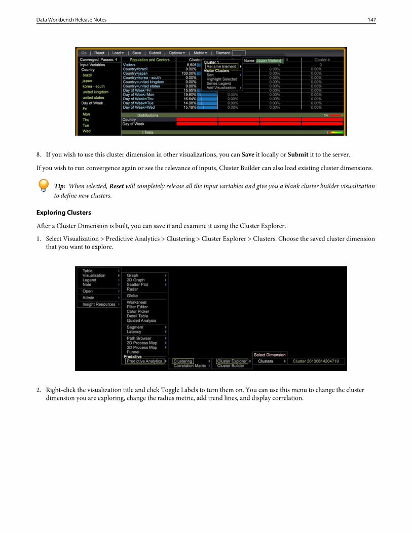
8. If you wish to use this cluster dimension in other visualizations, you can Save it locally or Submit it to the server.
If you wish to run convergence again or see the relevance of inputs, Cluster Builder can also load existing cluster dimensions.
Tip: When selected, Reset will completely release all the input variables and give you a blank cluster builder visualizationto define new clusters.
Exploring Clusters
After a Cluster Dimension is built, you can save it and examine it using the Cluster Explorer.
1. Select Visualization > Predictive Analytics > Clustering > Cluster Explorer > Clusters. Choose the saved cluster dimensionthat you want to explore.
2. Right-click the visualization title and click Toggle Labels to turn them on. You can use this menu to change the clusterdimension you are exploring, change the radius metric, add trend lines, and display correlation.
147Data Workbench Release Notes
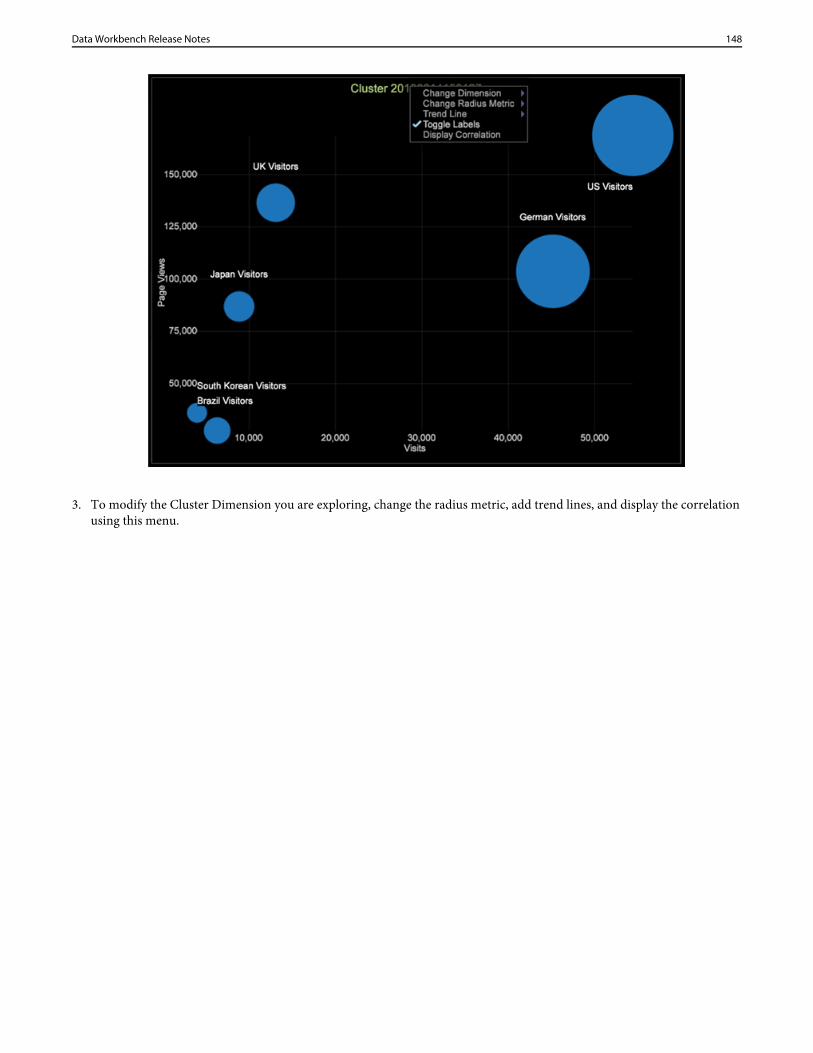
3. To modify the Cluster Dimension you are exploring, change the radius metric, add trend lines, and display the correlationusing this menu.
148Data Workbench Release Notes
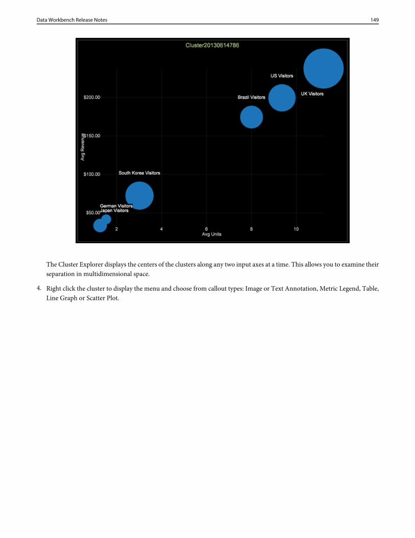
The Cluster Explorer displays the centers of the clusters along any two input axes at a time. This allows you to examine theirseparation in multidimensional space.
4. Right click the cluster to display the menu and choose from callout types: Image or Text Annotation, Metric Legend, Table,Line Graph or Scatter Plot.
149Data Workbench Release Notes
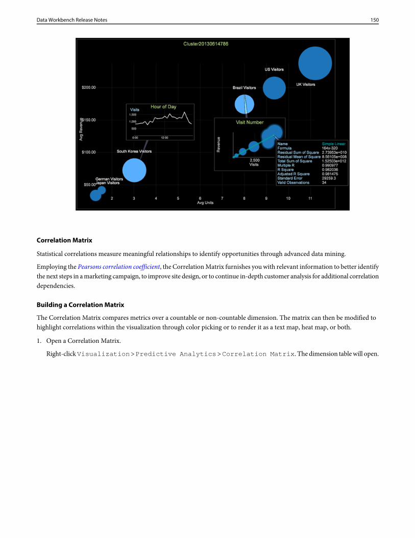
Correlation Matrix
Statistical correlations measure meaningful relationships to identify opportunities through advanced data mining.
Employing the Pearsons correlation coefficient, the Correlation Matrix furnishes you with relevant information to better identifythe next steps in a marketing campaign, to improve site design, or to continue in-depth customer analysis for additional correlationdependencies.
Building a Correlation Matrix
The Correlation Matrix compares metrics over a countable or non-countable dimension. The matrix can then be modified tohighlight correlations within the visualization through color picking or to render it as a text map, heat map, or both.
1. Open a Correlation Matrix.
Right-click Visualization > Predictive Analytics > Correlation Matrix. The dimension table will open.
150Data Workbench Release Notes
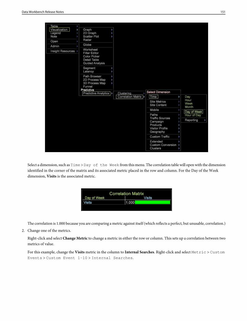
Select a dimension, such as Time > Day of the Week from this menu. The correlation table will open with the dimensionidentified in the corner of the matrix and its associated metric placed in the row and column. For the Day of the Weekdimension, Visits is the associated metric.
The correlation is 1.000 because you are comparing a metric against itself (which reflects a perfect, but unusable, correlation.)
2. Change one of the metrics.
Right-click and select Change Metric to change a metric in either the row or column. This sets up a correlation between twometrics of value.
For this example, change the Visits metric in the column to Internal Searches. Right-click and select Metric > CustomEvents > Custom Event 1-10 > Internal Searches.
151Data Workbench Release Notes
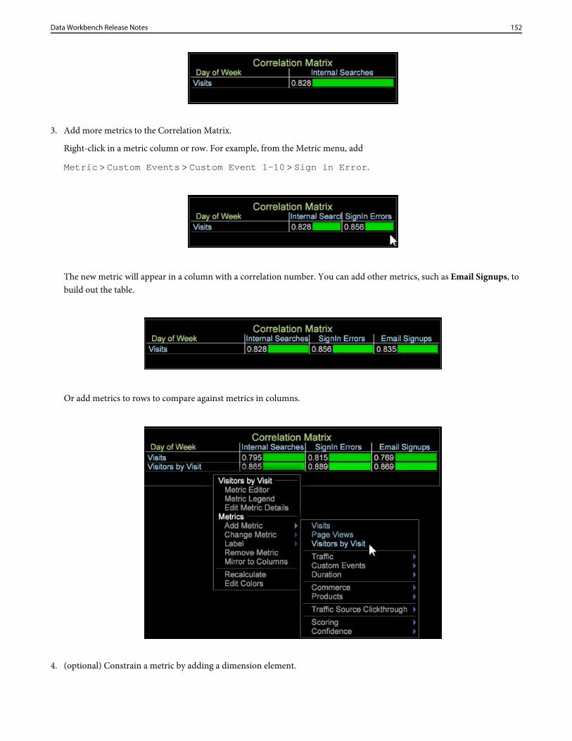
3. Add more metrics to the Correlation Matrix.
Right-click in a metric column or row. For example, from the Metric menu, add
Metric > Custom Events > Custom Event 1-10 > Sign in Error.
The new metric will appear in a column with a correlation number. You can add other metrics, such as Email Signups, tobuild out the table.
Or add metrics to rows to compare against metrics in columns.
4. (optional) Constrain a metric by adding a dimension element.
152Data Workbench Release Notes
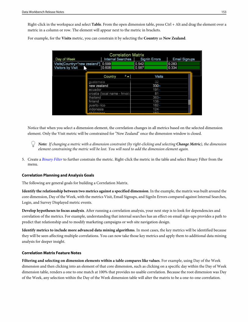
Right-click in the workspace and select Table. From the open dimension table, press Ctrl + Alt and drag the element over ametric in a column or row. The element will appear next to the metric in brackets.
For example, for the Visits metric, you can constrain it by selecting the Country as New Zealand.
Notice that when you select a dimension element, the correlation changes in all metrics based on the selected dimensionelement. Only the Visit metric will be constrained for "New Zealand" once the dimension window is closed.
Note: If changing a metric with a dimension constraint (by right-clicking and selecting Change Metric), the dimensionelement constraining the metric will be lost. You will need to add the dimension element again.
5. Create a Binary Filter to further constrain the metric. Right-click the metric in the table and select Binary Filter from themenu.
Correlation Planning and Analysis Goals
The following are general goals for building a Correlation Matrix.
Identify the relationship between two metrics against a specified dimension. In the example, the matrix was built around thecore dimension, Day of the Week, with the metrics Visit, Email Signups, and SignIn Errors compared against Internal Searches,Login, and Survey Displayed metric events.
Develop hypotheses to focus analysis. After running a correlation analysis, your next step is to look for dependencies andcorrelation of the metrics. For example, understanding that internal searches has an effect on email sign-ups provides a path topredict that relationship and to modify marketing campaigns or web site navigation design.
Identify metrics to include more advanced data mining algorithms. In most cases, the key metrics will be identified becausethey will be seen affecting multiple correlations. You can now take those key metrics and apply them to additional data mininganalysis for deeper insight.
Correlation Matrix Feature Notes
Filtering and selecting on dimension elements within a table compares like values. For example, using Day of the Weekdimension and then clicking into an element of that core dimension, such as clicking on a specific day within the Day of Weekdimension table, renders a one to one match at 100% that provides no usable correlation. Because the root dimension was Dayof the Week, any selection within the Day of the Week dimension table will alter the matrix to be a one-to-one correlation.
153Data Workbench Release Notes
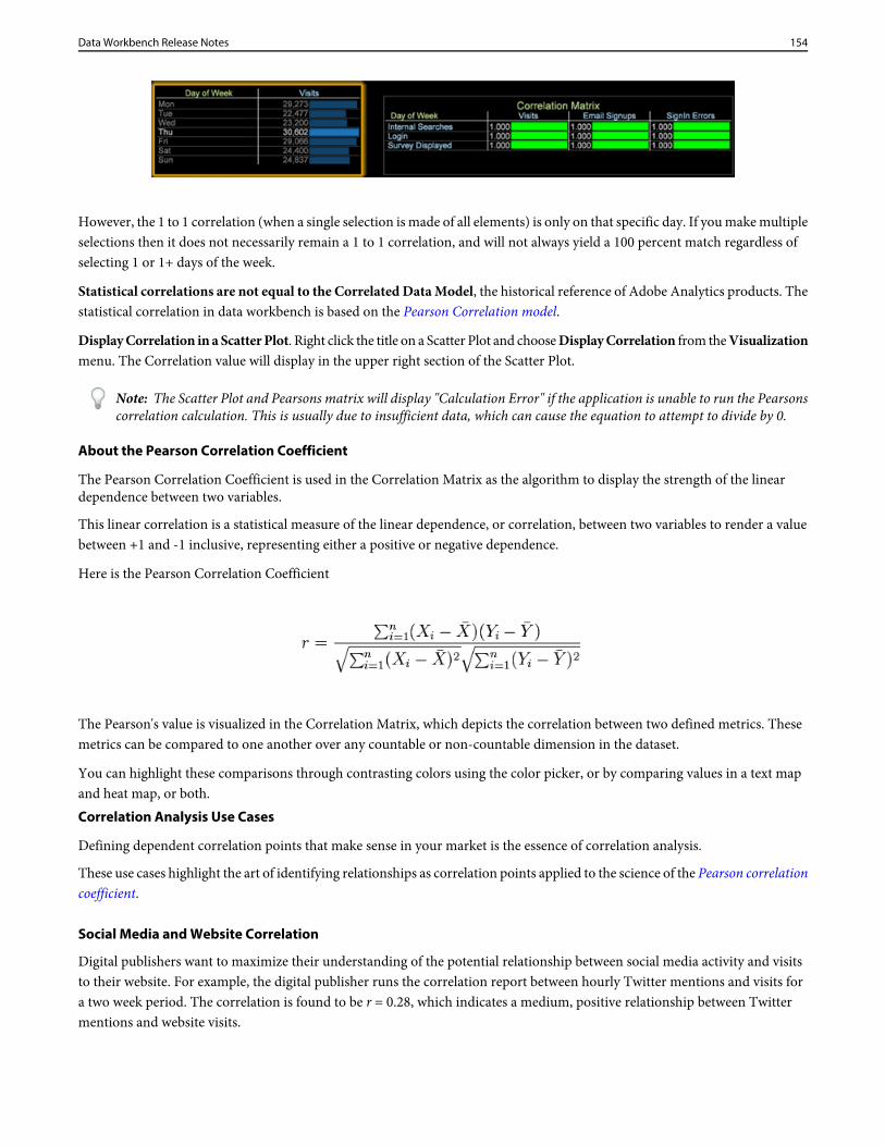
However, the 1 to 1 correlation (when a single selection is made of all elements) is only on that specific day. If you make multipleselections then it does not necessarily remain a 1 to 1 correlation, and will not always yield a 100 percent match regardless ofselecting 1 or 1+ days of the week.
Statistical correlations are not equal to the Correlated Data Model, the historical reference of Adobe Analytics products. Thestatistical correlation in data workbench is based on the Pearson Correlation model.
Display Correlation in a Scatter Plot. Right click the title on a Scatter Plot and choose Display Correlation from the Visualizationmenu. The Correlation value will display in the upper right section of the Scatter Plot.
Note: The Scatter Plot and Pearsons matrix will display "Calculation Error" if the application is unable to run the Pearsonscorrelation calculation. This is usually due to insufficient data, which can cause the equation to attempt to divide by 0.
About the Pearson Correlation Coefficient
The Pearson Correlation Coefficient is used in the Correlation Matrix as the algorithm to display the strength of the lineardependence between two variables.
This linear correlation is a statistical measure of the linear dependence, or correlation, between two variables to render a valuebetween +1 and -1 inclusive, representing either a positive or negative dependence.
Here is the Pearson Correlation Coefficient
The Pearson's value is visualized in the Correlation Matrix, which depicts the correlation between two defined metrics. Thesemetrics can be compared to one another over any countable or non-countable dimension in the dataset.
You can highlight these comparisons through contrasting colors using the color picker, or by comparing values in a text mapand heat map, or both.Correlation Analysis Use Cases
Defining dependent correlation points that make sense in your market is the essence of correlation analysis.
These use cases highlight the art of identifying relationships as correlation points applied to the science of the Pearson correlationcoefficient.
Social Media and Website Correlation
Digital publishers want to maximize their understanding of the potential relationship between social media activity and visitsto their website. For example, the digital publisher runs the correlation report between hourly Twitter mentions and visits fora two week period. The correlation is found to be r = 0.28, which indicates a medium, positive relationship between Twittermentions and website visits.
154Data Workbench Release Notes
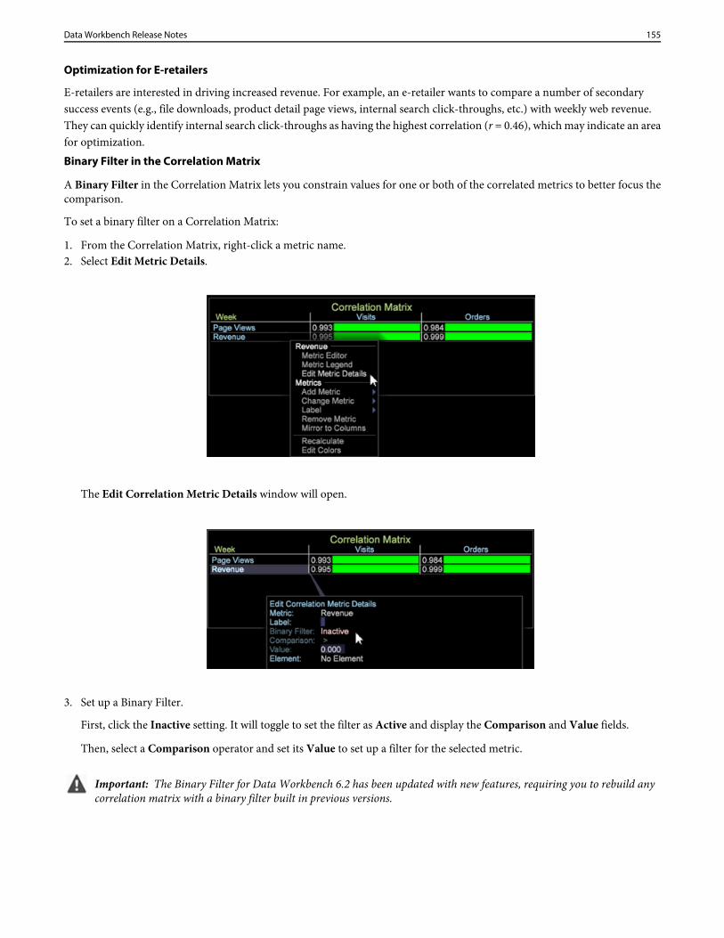
Optimization for E-retailers
E-retailers are interested in driving increased revenue. For example, an e-retailer wants to compare a number of secondarysuccess events (e.g., file downloads, product detail page views, internal search click-throughs, etc.) with weekly web revenue.They can quickly identify internal search click-throughs as having the highest correlation (r = 0.46), which may indicate an areafor optimization.Binary Filter in the Correlation Matrix
A Binary Filter in the Correlation Matrix lets you constrain values for one or both of the correlated metrics to better focus thecomparison.
To set a binary filter on a Correlation Matrix:
1. From the Correlation Matrix, right-click a metric name.2. Select Edit Metric Details.
The Edit Correlation Metric Details window will open.
3. Set up a Binary Filter.
First, click the Inactive setting. It will toggle to set the filter as Active and display the Comparison and Value fields.
Then, select a Comparison operator and set its Value to set up a filter for the selected metric.
Important: The Binary Filter for Data Workbench 6.2 has been updated with new features, requiring you to rebuild anycorrelation matrix with a binary filter built in previous versions.
155Data Workbench Release Notes
Adding Dimension Elements
You can also add a dimension element to constrain a metric. A metric can have only one element associated with it.
Right-click in the workspace and select Table. Open a dimension with its elements and drag to the Element setting in the EditCorrelation Metric Details window, or drop on a metric in the Correlation Matrix.
DeviceAtlas Transformation Distribution
The DeviceAtlas JSON file will now be distributed in a .bundle file (renamed .tar.gz) along with DeviceAtlas.dlland DeviceAtlas64.dll files.
When the administrator upgrades the server to version 6.0, the DeviceAtlas.bundle file is included with the upgradepackage in the Software and Docs profile (softdocs profile) located at:
Server Packages > v6.00 > Server_6.00.zip
The DeviceAtlas.bundle file is extracted to Server\Lookups\DeviceAtlas.
The DeviceAtlas.bundle file should be placed in a directory that is synchronized to the DPUs, and the DeviceAtlas.cfgfile corresponding to the new DeviceAtlasComponent should be placed in the "Components for Processing Servers" directoryon the synchronization master. When the DeviceAtlas.bundle file is changed, the very next DeviceAtlas lookup call will getresults based on the updated API and/or JSON file.
Modify the Transformation.cfg file
The DeviceAtlas Transformations will no longer need to specify the path to the JSON file. Any previous DeviceAtlasTransformationthat is defined in the transformation.cfg file should no longer include the File parameter that points to the obfuscated JSON file.
This example Transformation.cfg file shows the File argument that should be deleted to avoid confusion. (Leaving it there willnot cause harm, but only potential confusion because it will be ignored.)6 = DeviceAtlasTransformation: Comments = Comment: 0 items Condition = AndCondition: 0 items
File = string: Lookups\\DeviceAtlas\\20110106_private.json.obfuscated ^^ DELETE THE ABOVE LINE FROM ALL PREVIOUS TRANSFORMATIONS ^^
Name = string: DeviceAtlas Lookup Outputs = vector: 4 items
156Data Workbench Release Notes
0 = Column: Column Name = string: vendor Field Name = string: x-vendor 1 = Column: Column Name = string: model Field Name = string: x-model 2 = Column: Column Name = string: isBrowser Field Name = string: x-isbrowser 3 = Column: Column Name = string:usableDisplayHeight Field Name = string: x-usable-display-heightUser Agent = string: x-ua
Modify the DeviceAtlas.cfg file
This is an example of the component argument required in the DeviceAtlas.cfg file.component = DeviceAtlasComponent: DeviceAtlas Bundle File = string:Lookups\\DeviceAtlas\\DeviceAtlas.bundle Unsynchronized Bundle Extraction Path = string: Temp\\DeviceAtlas\\
This DeviceAtlas.bundle file will be treated just like a configuration file from the perspective of the Profile Synchronizationfeature. In addition, the JSON data and DLL will be used at the Component level rather than at the individual Transformationlevel.
A new DeviceAtlasComponent, upon startup, finds the .bundle conglomeration, de-obfuscates the JSON file into memory,extracts the files into a temporary directory, and loads the appropriate DLL for the running platform. This component alsomonitors changes to the bundle file, and reloads the DLL and .cfg file automatically if it changes.
Running DeviceAtlas
Proper configuration makes a big difference in the time required for transformation. The transformation can be configured torun only once per visitor per session to allow DeviceAtlas to speed up the process.
If deployed using Log Processing.cfg:
Run the transformations twice.
1. Look up only the mobile id field, then2. Create conditions to ignore the mobile id and then look up the rest of the fields.
If deployed using Transformation.cfg:Deploy as in Step 1 in Log Processing above, or use cross-rows to support a conditional setting.
• Cross-Rows—Grab the previous session key. Then identify if the current session key is different from the one found withcross-rows. If so, then the DeviceAtlas transformation will only run on one record per session.
Data Workbench 6.0.4 Release Notes
New features introduced in Data Workbench 6.0.4, including bug fixes and known issues.
To view previous features and fixes based for each past release, see the release note archives.
New FeaturesData Workbench 6.0.4 includes these new features and visualizations for added reporting capabilities and predictive analysistools.
157Data Workbench Release Notes
Propensity Scoring visualization. Data workbench calculates scores for each visitor as an estimated probability that a specifiedevent may happen. The Visitor Scoring visualization allows you to create a score dimension that gives a probability of a specifiedevent for every visitor of interest based on the input variables.
See Propensity Scoring for additional information about this feature.
Upgrade Requirements
Log Source ID must be defined. Starting in version 6.04, if the Log Source ID is not defined then you will get the followingerror:Missing Log Souce ID in log processing.cfg. Log Source ID must be defined for all log sources.
The Recording of Rows per Log Source was added in Data Workbench 6.0 and can be defined in the custom profile LogProcessing.cfg by adding a uniquely named Log Source ID. If you have a blank Log Source ID, then you could see Log Processingissues such as incomplete reading of the log source data and other discrepancies.Log Processing.cfgLog Sources = vector: 2 items 0 = VisualSensor: Compressed = bool: false Log Paths = vector: 1 items 0 = Path: \some path\ Log Server = serverInfo: Address = string: Name = string: Port = int: 80 Proxy Address = string: Proxy Password = string: Proxy Port = int: 8080 Proxy User Name = string: SSL Client Certificate = string: Certificates\\server_cert.pem SSL Server Common Name = string: Use SSL = bool: false
Log Source ID = string: <Name your ID Here>
158Data Workbench Release Notes
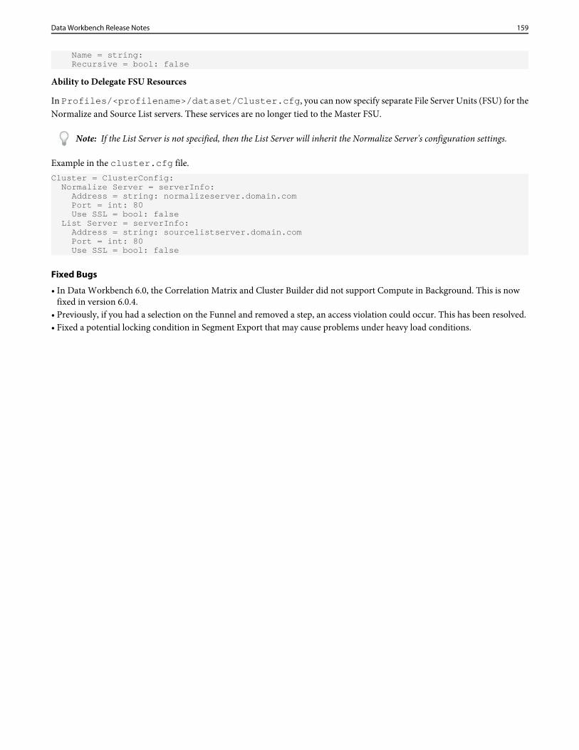
Name = string: Recursive = bool: false
Ability to Delegate FSU Resources
In Profiles/<profilename>/dataset/Cluster.cfg, you can now specify separate File Server Units (FSU) for theNormalize and Source List servers. These services are no longer tied to the Master FSU.
Note: If the List Server is not specified, then the List Server will inherit the Normalize Server's configuration settings.
Example in the cluster.cfg file.Cluster = ClusterConfig: Normalize Server = serverInfo: Address = string: normalizeserver.domain.com Port = int: 80 Use SSL = bool: false List Server = serverInfo: Address = string: sourcelistserver.domain.com Port = int: 80 Use SSL = bool: false
Fixed Bugs
• In Data Workbench 6.0, the Correlation Matrix and Cluster Builder did not support Compute in Background. This is nowfixed in version 6.0.4.
• Previously, if you had a selection on the Funnel and removed a step, an access violation could occur. This has been resolved.• Fixed a potential locking condition in Segment Export that may cause problems under heavy load conditions.
159Data Workbench Release Notes