Dynamical origin of low-frequency variability in a highly

nonlinear mid-latitude coupled model

S. Kravtsov1, 5, P. Berlo!2, W. K. Dewar3, M. Ghil4, 5 and J. C. McWilliams5

J. Climate, sub judice

April 20, 2006

1Corresponding author address: Dr. Sergey Kravtsov, Department of Mathematical Sciences, Uni-versity of Wisconsin-Milwaukee, P.O. Box 413, Milwaukee, WI 53201. E-mail: kravtsov@uwm.edu

2 Physical Oceanography Department, Woods Hole Oceanographic Institute, Woods Hole, MA02543

3Department of Oceanography, Florida State University, Tallahassee, FL 32306-30484Department Terre–Atmosphere–Ocean and Laboratoire de Meteorologie Dynamique (CNRS and

IPSL), Ecole Normale Superieure, Paris5 Department of Atmospheric and Oceanic Sciences and Institute of Geophysics and Planetary

Physics, University of California-Los Angeles, Los Angeles, CA 90095

Abstract

A novel mechanism of decadal mid-latitude coupled variability, which crucially depends on the

nonlinear dynamics of both the atmosphere and the ocean, is presented. The coupled model

studied involves quasi-geostrophic atmospheric and oceanic components, which communicate

with each other via a constant-depth oceanic mixed layer. A series of coupled and uncoupled

experiments show that the decadal coupled mode is active across parameter ranges that allow

the bimodality of the atmospheric zonal flow to coexist with oceanic turbulence. The latter

is most intense in the regions of inertial recirculation (IR). Bimodality is associated with the

existence of two distinct anomalously persistent zonal-flow modes, which are characterized by

di!erent latitudes of the atmospheric jet stream. IR reorganizations caused by transitions of

the atmosphere from its high-latitude to its low-latitude state and vice-versa create sea-surface

temperature anomalies that tend to induce transition to the opposite atmospheric state. The

decadal-to-interdecadal time scale of the resulting oscillation is set by the IR adjustment; the

latter depends most sensitively on the oceanic bottom drag. The period T of the nonlinear

oscillation is of 7–25 yr for the range of parameters explored, with the most realistic parameter

values yielding T ! 20 yr.

Aside from this nonlinear oscillation, an interannual Rossby wave mode is present in all

coupled experiments. This coupled mode depends neither on atmospheric bimodality, nor on

ocean-eddy dynamics; it is analogous to the mode found previously in a channel configuration.

Its time scale in the model with a closed ocean basin is set by cross-basin wave propagation

and equals 3–5 yr for a basin width comparable with the North Atlantic.

1

1 . Introduction

a. Motivation

A major ambiguity in prescribing any portion of the climate change to mid-latitude coupled

dynamics stems from apparent failure of the general circulation models (GCMs) to detect a

robust and statistically significant atmospheric response to weak, ocean-induced sea-surface

temperature (SST) anomalies (Kushnir and Held 1996; Saravanan 1998; Rodwell et al. 1999;

Mehta et al. 2000). We hypothesize here that, in order to be conducive to mid-latitude coupled

variability, an atmospheric model must necessarily be characterized by a strongly nonlinear

behavior, which will allow small perturbations of external (SST) forcing to cause substantial

low-frequency reorganizations of atmospheric flow patterns. A conceptual way to think about

GCMs not supporting mid-latitude coupled modes would then be to say that they likely operate

in a linear regime (which may be quite realistic, of course). Another feature of GCMs which

reduces their potential for active mid-latitude coupled dynamics, and which can also, in this

case, be more easily criticized from a dynamical perspective, has to do with coarse resolutions of

the GCMs’ oceanic components, a consequence of which is the appearance of relatively smooth,

laminar ocean circulations. The ocean, though, is characterized by energetic variability and

nonlinear behavior. The clear significance of such turbulence in the ocean calls into question

the results of coupled GCM results conducted in the absence of these dynamics.

In order to address the above hypotheses, we study the behavior of a coupled ocean–

atmosphere numerical model, in which both atmospheric and oceanic components are governed

by quasi-geostrophic (QG) dynamics at spatial resolutions that allow vigorous intrinsic vari-

ability in both fluids. In the ocean, this variability is concentrated in and near the eastward

jet formed by the merger of the separated western boundary currents and the adjacent inertial

recirculation (IR) region (see Holland 1978; we use essentially the same model for our exper-

2

imentation). This region is characterized by two strong vortices of opposite sign, on either

side of the separated eastward jet, whose transports exceed those in the Sverdrup interior by a

factor of 3–4. A feature of the atmospheric component of the model (which is identical to that

of Kravtsov et al. 2005a) of considerable importance to the present study is that in certain pa-

rameter ranges of the surface drag coe"cient k, the model’s intrinsic low-frequency variability

(LFV) consists of irregular transitions between two anomalously persistent, high-latitude and

low-latitude jet states, which we will refer to as the atmospheric bimodality.

In our control case, we will use the value of k!1 = 6.17 days, for which the intrinsic transi-

tions to the atmospheric low-latitude state are frequent, but irregular in the uncoupled atmo-

spheric setting (see Kravtsov et al. 2005a). In our coupled model, however, where the ocean

and atmosphere exchange heat an momentum via a constant-depth mixed-layer of Kravtsov

and Robertson (2002), the frequency of these transitions varies in time and exhibits a broad

spectral peak centered at about 9 yr (not shown); the same spectral peak is present in the

oceanic time series (see Fig. 1).Fig. 1

The oscillation involves development of an intense ocean

eastward jet and vigorous IR vortices when the high-latitude atmospheric jet persists, while

the oceanic jet weakens and breaks down into eddies during the phase characterized by more

frequent atmospheric transitions to low-latitude state (Kravtsov et al. 2006).

The purpose of the present paper is to investigate the dynamics of this behavior by carrying

out and analyzing various uncoupled integrations and studying the sensitivity to oceanic and

atmospheric parameters, most notably to the atmospheric surface drag coe"cient and the

oceanic bottom drag, as well as to the ocean model’s horizontal resolution. The former, as

we have already pointed out, controls atmospheric bimodality, while the latter two impose

restrictions on the oceanic turbulence. The suite of the proposed experiments is thus designed

to establish (i) whether the behavior is inherently coupled and (ii) whether the atmospheric

3

bimodality and oceanic turbulence are essential for this behavior.

b. Summary of experiments and road map

We summarize the major experiments we have performed in Table 1.Table 1

Experiment (1) is

the control run, which uses high value of oceanic bottom drag (an equivalent depth of bottom

Ekman layer Df = 30 m) and an intermediate atmospheric surface drag of k!1 = 6.17 days.

Experiments (2) and (3) are identical to Exp. (1) except for the value of the atmospheric

surface drag, which is respectively lower and higher than that in the control run. Experiments

(4–6) are analogous to Exps. (1–3), but use a coarser-resolution ocean model and, hence, higher

horizontal viscosity, while Exp. (7) uses the resolution and viscosity of the control run, but a

value of the ocean bottom drag coe"cient that is 10 times smaller (Df = 3 m). Thus, Exps.

(1–7) all use a fully coupled model. We will see, however, that coarse-resolution experiments

do not support the coupled mode of the control run, while the period of this mode increases as

the ocean bottom drag is reduced. Both of these properties suggest that the ocean eddies are

essential to the oscillation.

The remainder of the experiments are uncoupled. Experiments (8–11) are designed to estab-

lish the coupled nature of the phenomenon under consideration. Experiment (8) is an ocean-only

integration forced by surrogate atmospheric pumping, which consists of a constant, time-mean

field and a stochastic component obtained by fitting a linear stochastic model (Kravtsov et al.

2005b) to the history of this forcing from the fully coupled run (Exp. 1). Experiments (9–11)

use time-mean ocean circulation from Exps. (1–3), respectively, to force the atmosphere–

ocean-mixed-layer model. The decadal oscillatory behavior is not realized in any of the above

uncoupled integrations, and we conclude that coupled dynamics are at play (a spectral peak at

a period of about 4-5 yr appears, though, in all coupled experiments [see, for example, Fig. 1],

and is associated with a coupled Rossby wave mode [see section 5]).

4

In order to show how the atmosphere responds to ocean-induced SST anomalies, Experiment

12 uses composites of ocean circulation keyed to phase categories of the 9-yr cycle of Exp. (1)

(see section 2b) to force the atmosphere–ocean-mixed-layer model and documents changes in

conditional probability of the atmospheric low-latitude state. Finally, to clarify the role of

ocean eddies in setting up the coupled oscillation’s time scale, ocean adjustment experiments

Exps. (13–15) use ocean-QG-interior coupled to ocean-mixed-layer model forced by composites

of atmospheric circulation in the high-latitude state for 100 yr, low-latitude state for another

100 yr and, again, 100 yr of high-latitude state. (These experiments used models from Exp.

(2), (5), and (7), respectively. Atmospheric composites were computed as described in section

2b). They will demonstrate that (i) the major di!erence between the adjustment of high-

resolution, eddy-rich ocean (Exp. 13) versus its coarse-resolution counterpart (Exp. 14) is the

lack of eddy-induced SST anomalies in the latter; and (ii) that the oscillation period (in Exps.

1 and 7) scales as the eddy-driven adjustment time scale (as determined by Exp. 13 and 15,

respectively).

The paper is organized as follows. In section 2, we describe the analysis methods we have

used. Sections 3 and 4 focus on the roles of atmospheric and oceanic nonlinearity in the

coupled oscillation, respectively. The linear coupled Rossby wave mode is described in section

5. Concluding remarks follow in section 6.

2 . Methods

a. Spectral analysis

We applied to the oceanic and atmospheric time series two complementary methods of ad-

vanced spectral analysis (Ghil et al. 2002): the multi-taper method (MTM: Thomson 1982,

1990; Mann and Lees 1996) and singular spectrum analysis (SSA: Vautard and Ghil 1989; Det-

5

tinger et al. 1995). These methods provide more accurate and reliable detection of periodicity

in a given time series compared to traditional Fourier methods, and SSA also provides more

consistent compositing procedures.

1) MULTI-TAPER METHOD

MTM replaces the single window used in Fourier analysis by a small set of optimal windows

(tapers) that objectively minimize power leakage and reduce uncertainties in the estimated

spectra. Statistical significance against a red-noise null hypothesis is assessed by fitting an

AR(1) process to the time series being tested (Mann and Lees 1996). To concentrate on

decadal variability, we first took one-year-long nonoverlapping box-car averages of a given time

series and used 3 tapers to compute MTM spectra, resulting in a spectral resolution of 0.02

cycle/yr.

2) SINGULAR-SPECTRUM ANALYSIS (SSA)

SSA computes the eigenvalues and eigenvectors of a given time series’ lag-covariance ma-

trix. These eigenvalues and eigenvectors are also called the singular values of the time series

and the temporal empirical orthogonal functions (T-EOFs), respectively. The projection of the

original time series onto T-EOFs yields temporal principal components (T-PCs). An oscillatory

component is represented in SSA by a single pair of approximately equal singular values, with

respective temporal EOFs and PCs in phase quadrature (Vautard and Ghil 1989); its char-

acteristic frequency is estimated by maximizing the correlation with a sinusoid. To eliminate

spurious pairs, we have applied three tests: (i) a !2-test against a red-noise null hypothesis

(Allen and Smith 1996); (ii) a lag-correlation test to verify that two given PCs are indeed in

quadrature (Ghil and Mo 1991); and (iii) the “same frequency” and “strong FFT” tests of

Vautard et al. (1992). In each case, we have used the 40-day binning and applied an SSA

window width of 365" 40 days = 40 yr.

The same statistically significant oscillations were detected in most cases when we applied

6

a generalization of SSA to a time series of vectors, the so-called multichannel SSA (M-SSA:

Keppenne and Ghil 1993; Plaut and Vautard 1994; Ghil et al. 2002), to the combined atmo-

spheric and ocean time series. We also computed the reconstructed components (RCs) of the

oscillation. The RCs are narrow-band versions of the time series, where the band filters are

derived data-adaptively from the time series itself in order to maximize the variance captured

(Ghil and Vautard 1991; Vautard et al. 1992).

For each time series we have considered, the two complementary methods of spectral analysis

described above have identified the same statistically significant periodicities.

b. Compositing

For each detected oscillation, we obtained its composite cycle in a given oceanic or atmo-

spheric scalar quantity or field by dividing the RC time series obtained by M-SSA into eight

phases, and averaging each field under consideration over the days belonging to each phase.

The time series we used for defining the eight phases were, typically, the atmospheric jet posi-

tion and the oceanic kinetic energy, and each of the eight phases contained the same amount

of data points.

We applied the same compositing methodology to obtain atmospheric high-latitude and

low-latitude jet regime patterns for the use in ocean-only adjustment experiments. In this case,

we first computed the probability density function (PDF) of the atmospheric jet’s latitude by

binning its values into 30 equal segments and counting the number of days the model spent

within each segment, divided by the total number of data points in the time series. The

PDF was typically strongly skewed and well represented as a sum of two Gaussians. The

atmospheric regimes were computed by compositing the points in the neighborhood of each of

the two Gaussians.

7

c. Lagged covariance analysis

We will use this analysis in section 5 to describe the model’s coupled Rossby wave mode. In

this approach, we regress the model fields onto the time series of ocean kinetic energy, centered,

normalized and filtered in the 1–10-yr band; multiplying the filtered time series so obtained

by #1 has the field at lag 0 correspond to an ocean state with minimum kinetic energy. The

convention we use is that the fields at negative lags are the patterns that arise prior to the

minimum of the kinetic energy and those at positive lags follow the minimum of kinetic energy.

3 . Nonlinear atmospheric sensitivity

In this section, we explore dependence of the coupled decadal-to-interdecadal mode on atmo-

spheric bimodality and establish the ways in which the ocean a!ects atmospheric circulation

nonlinearly, by changing the attractor basin of the atmosphere’s low-latitude state.

a. Sensitivity to atmospheric surface friction

The PDFs of atmospheric jet position for the coupled experiments using lower and higher

values of surface friction (Exps. 2 and 3 of Table 1) are shown in Fig. 2.Fig. 2

The PDF based on

data from Exp. 2 exhibits pronounced bimodality, while there is considerable skewness, but no

multiple PDF maxima in Exp. 3; the control run’s (Exp. 1) PDF has the skewness in between

the values characterizing Exps. 2 and 3. This skewness is still indicative of the presence of

two dynamically distinct states, or modes, namely high-latitude and low-latitude atmospheric

states (see Kravtsov et al. 2005a).

An MTM-based spectral analysis of ocean kinetic energy time series from Exps. 2 and 3 is

shown in Fig. 3.Fig. 3

This analysis does identify both the 4-yr and 10-yr peaks for Exp. 3 and

a similar 4-yr peak, but no decadal peak in Exp. 2. The decadal peak in Exp. 3 is slightly

8

shifted with respect to the 9-yr peak in the control run (Exp. 1). Similarly, interannual peak

in the control run at 5 yr is slightly shifted with respect to 4-yr peaks of Exps. 2 and 3.

The interannual peak with a period of 4–5 yr is, in fact, present in all coupled experiments

listed in Table 1, as identified by both MTM and SSA analysis of the oceanic kinetic energy

(not shown). In contrast, no uncoupled integration exhibits such a peak (see Table 1). This

signal is associated with a coupled propagating Rossby wave, which will be described in greater

detail in section 5. This wave does not induce significant variations of the atmospheric jet

position, hence none of the spectra of the latter quantity exhibit such a peak (not shown).

An interannual spectral peak in the atmospheric circulation is, however, captured by applying

first traditional PC analysis in space (Preisendorfer 1988) to the monthly-mean atmospheric

streamfunction. The resulting EOFs 2 and 3 have a wave-4 spatial pattern and the associated

PCs exhibit a 4-5-yr spectral peak (not shown).

An analysis of Exp. 3 (high surface drag), similar to that performed in Kravtsov et al. (2006)

for the control run, shows that the decadal oscillation identified in the spectra of Figs. 1 and 3b

here has the same spatial and temporal characteristics (not shown) as the decadal oscillation of

the control run, although it is responsible for a smaller fraction of the model’s variance. As the

surface friction parameter increases further and the atmospheric model becomes less and less

bimodal (see Kravtsov et al. 2005a), the coupled nonlinear oscillation disappears altogether,

along with nonlinear atmospheric sensitivity to ocean-induced SST anomalies.

The absence of the coupled nonlinear oscillation from Exp. 2 with low atmospheric surface

drag (Fig. 3a) is somewhat surprising, in the light of our arguments about the role of atmo-

spheric bimodality in this oscillation. The apparent contradiction has to do with the number

of atmospheric jet transitions to the low-latitude state at low values of bottom drag. Figures

4(a–c)Fig. 4

show 200-yr-long segments of the atmospheric jet position simulated in Exps. 2, 1, and

3, respectively.

9

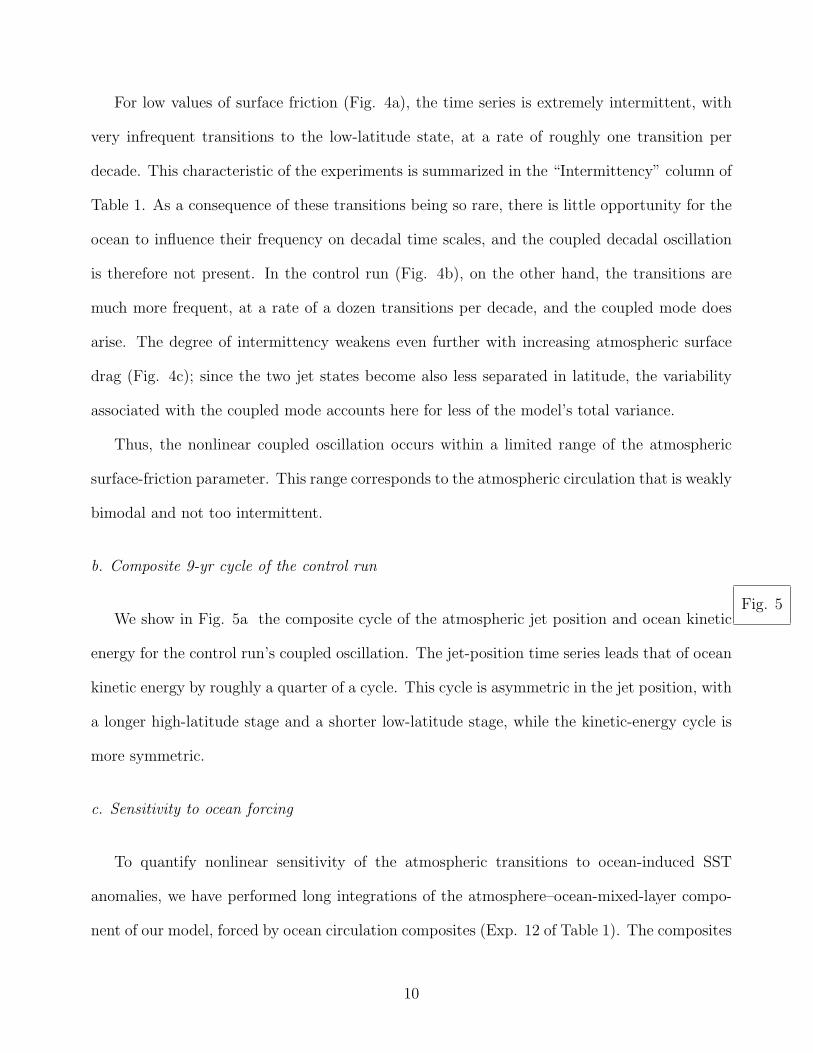
For low values of surface friction (Fig. 4a), the time series is extremely intermittent, with

very infrequent transitions to the low-latitude state, at a rate of roughly one transition per

decade. This characteristic of the experiments is summarized in the “Intermittency” column of

Table 1. As a consequence of these transitions being so rare, there is little opportunity for the

ocean to influence their frequency on decadal time scales, and the coupled decadal oscillation

is therefore not present. In the control run (Fig. 4b), on the other hand, the transitions are

much more frequent, at a rate of a dozen transitions per decade, and the coupled mode does

arise. The degree of intermittency weakens even further with increasing atmospheric surface

drag (Fig. 4c); since the two jet states become also less separated in latitude, the variability

associated with the coupled mode accounts here for less of the model’s total variance.

Thus, the nonlinear coupled oscillation occurs within a limited range of the atmospheric

surface-friction parameter. This range corresponds to the atmospheric circulation that is weakly

bimodal and not too intermittent.

b. Composite 9-yr cycle of the control run

We show in Fig. 5aFig. 5

the composite cycle of the atmospheric jet position and ocean kinetic

energy for the control run’s coupled oscillation. The jet-position time series leads that of ocean

kinetic energy by roughly a quarter of a cycle. This cycle is asymmetric in the jet position, with

a longer high-latitude stage and a shorter low-latitude stage, while the kinetic-energy cycle is

more symmetric.

c. Sensitivity to ocean forcing

To quantify nonlinear sensitivity of the atmospheric transitions to ocean-induced SST

anomalies, we have performed long integrations of the atmosphere–ocean-mixed-layer compo-

nent of our model, forced by ocean circulation composites (Exp. 12 of Table 1). The composites

10

were keyed to the eight phases of the 9-yr oscillation in the control run (Exp. 1). We computed,

in each experiment, the probability of the low-latitude state, defined as the number of days

spent in this regime divided by the total number of days in the time series. The results are

shown in Fig. 5b.

The probability changes by about 10% of its mean value during the course of the oscillation;

the high-energy ocean state (Fig. 5a) is more likely to induce atmospheric transition to the low-

latitude regime and vice-versa. Thus, the atmospheric high-latitude jet state favors eastward

extension of the oceanic jet, and an overall more energetic ocean state (phases 2, 3, and 4 of Fig.

5a). This ocean state, in turn, favors more frequent atmospheric transitions to the low-latitude

state (Fig. 5b), and the negative swing of the coupled cycle begins (phases 5, 6, and 7 of Fig.

5a).

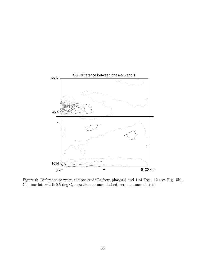
We examine next the SST anomalies that result in the changes of low-latitude jet occurrence

frequency, and plot in Fig. 6Fig. 6

the di!erence between the composite SST fields associated with

phases 5 and 1 of the oscillation in Exp. 12 (Figs. 5a,b). The increased probability of the

atmospheric low-latitude state is thus induced by the elongated, monopolar pattern of positive

SST anomalies centered roughly at the location of the climatological eastward jet extension

in the ocean. Similarly, negative SST anomalies in the oceanic jet-extension region induce

atmospheric preference for less frequent transitions to the low-latitude atmospheric state (not

shown).

Changes of 10% in the occurrence frequency of the low-latitude regime, like in Fig. 5b, as

well as SST anomaly patterns similar to that in Fig. 6 can in fact be obtained in atmosphere-

only simulations conditioned on the states of the coarse-resolution ocean model (not shown).

If this is the case, then why does the coarse-resolution ocean model, coupled to the same

atmospheric component, not exhibit the coupled decadal variability? We will show in section

4 that the SST forcing pattern of Fig. 6 in the higher-resolution ocean integration exhibits

11

increased persistence due to more active ocean eddies; this increased persistence is, therefore,

a primary reason for the existence of the coupled mode.

4 . Role of ocean nonlinearity

In this section, we consider the following two questions: “What determines the time scale of the

nonlinear coupled oscillation?” and “How important are ocean eddies in forcing SST patterns

that ensure e!ective ocean–atmosphere coupling?”

a. Ocean adjustment to switches between atmospheric forcing regimes

To test the hypothesis that the time scale of the coupled oscillation is set by nonlinear

oceanic adjustment to switches between high-latitude and low-latitude atmospheric forcing

regimes, we perform ocean adjustment experiments: Exps. 13–15 of Table 1 (see section 1b).

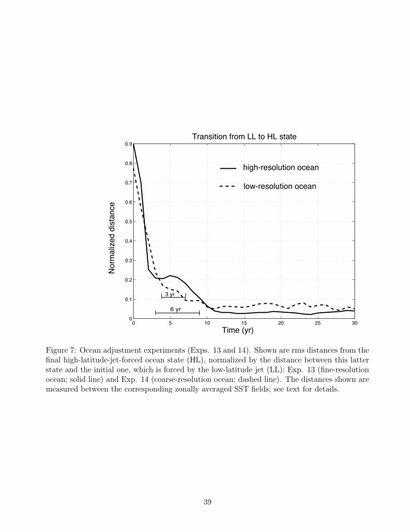
The results from Exps. 13 and 14 are plotted in Fig. 7Fig. 7

for the transition from the low-

latitude to the high-latitude forcing regime. Here we plot the root-mean-square (rms) distance

(defined as a Euclidean distance between two vectors, that is, the square root of the sum of

squared di!erences between corresponding components of the two vectors) between the vector

of instantaneous zonally averaged SST field and the vector of zonally averaged SST climatology

forced by the atmospheric high-latitude jet.

Prior to the analysis, we have applied a 5-yr running-mean filter to all the fields considered.

The results depend very little on the filter’s window size: they are qualitatively the same if 3-yr

or 7-yr filters are used instead (not shown). The distance plotted is normalized by the distance

between the time-averaged high-latitude and low-latitude states. Solid lines show the results

from Exp. 13, which uses the fine-resolution ocean, and light lines the results from Exp. 14

with coarser ocean resolution. In both cases, the distance decreases fairly rapidly over about

3–5 yr, from values of about 0.8–0.9 to values below 0.2. The asymptotic values below 0.1 are

12

reached after about 10 yr and di!er from zero due to the presence of intrinsic ocean variability

in the model.

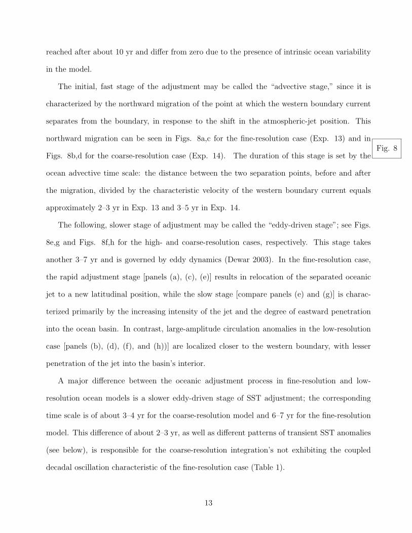
The initial, fast stage of the adjustment may be called the “advective stage,” since it is

characterized by the northward migration of the point at which the western boundary current

separates from the boundary, in response to the shift in the atmospheric-jet position. This

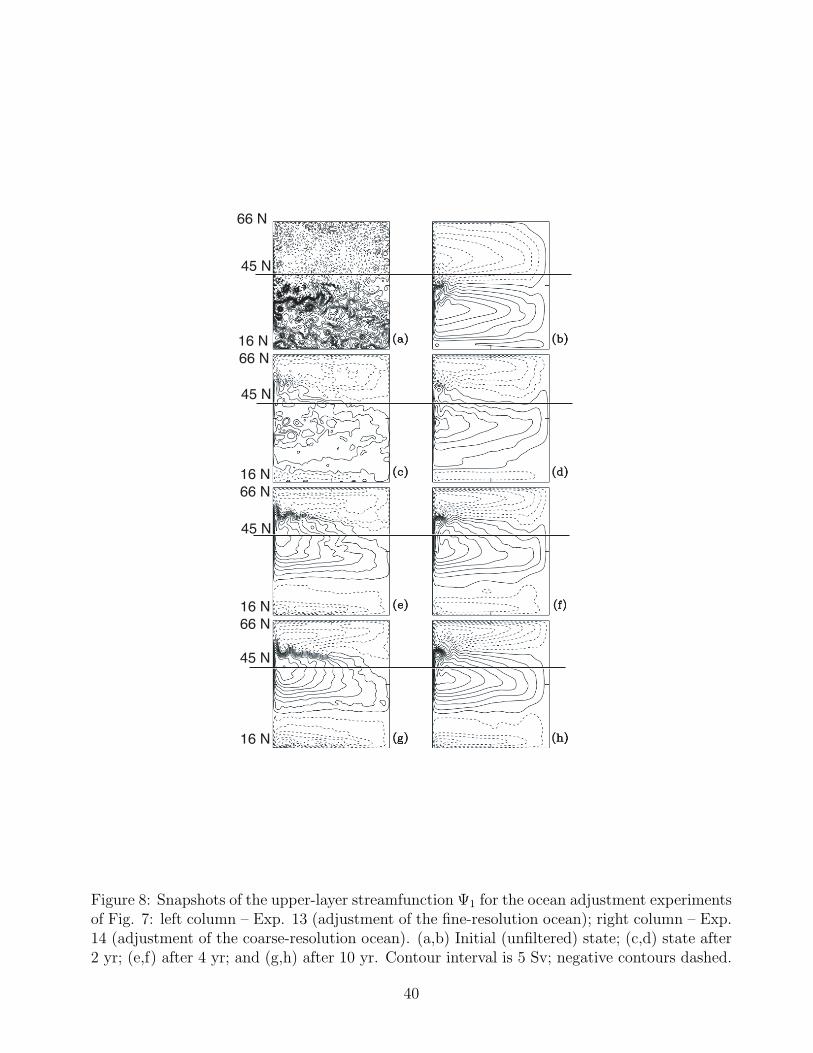
northward migration can be seen in Figs. 8a,c for the fine-resolution case (Exp. 13) and in

Figs. 8b,d for the coarse-resolution case (Exp. 14).Fig. 8

The duration of this stage is set by the

ocean advective time scale: the distance between the two separation points, before and after

the migration, divided by the characteristic velocity of the western boundary current equals

approximately 2–3 yr in Exp. 13 and 3–5 yr in Exp. 14.

The following, slower stage of adjustment may be called the “eddy-driven stage”; see Figs.

8e,g and Figs. 8f,h for the high- and coarse-resolution cases, respectively. This stage takes

another 3–7 yr and is governed by eddy dynamics (Dewar 2003). In the fine-resolution case,

the rapid adjustment stage [panels (a), (c), (e)] results in relocation of the separated oceanic

jet to a new latitudinal position, while the slow stage [compare panels (e) and (g)] is charac-

terized primarily by the increasing intensity of the jet and the degree of eastward penetration

into the ocean basin. In contrast, large-amplitude circulation anomalies in the low-resolution

case [panels (b), (d), (f), and (h))] are localized closer to the western boundary, with lesser

penetration of the jet into the basin’s interior.

A major di!erence between the oceanic adjustment process in fine-resolution and low-

resolution ocean models is a slower eddy-driven stage of SST adjustment; the corresponding

time scale is of about 3–4 yr for the coarse-resolution model and 6–7 yr for the fine-resolution

model. This di!erence of about 2–3 yr, as well as di!erent patterns of transient SST anomalies

(see below), is responsible for the coarse-resolution integration’s not exhibiting the coupled

decadal oscillation characteristic of the fine-resolution case (Table 1).

13

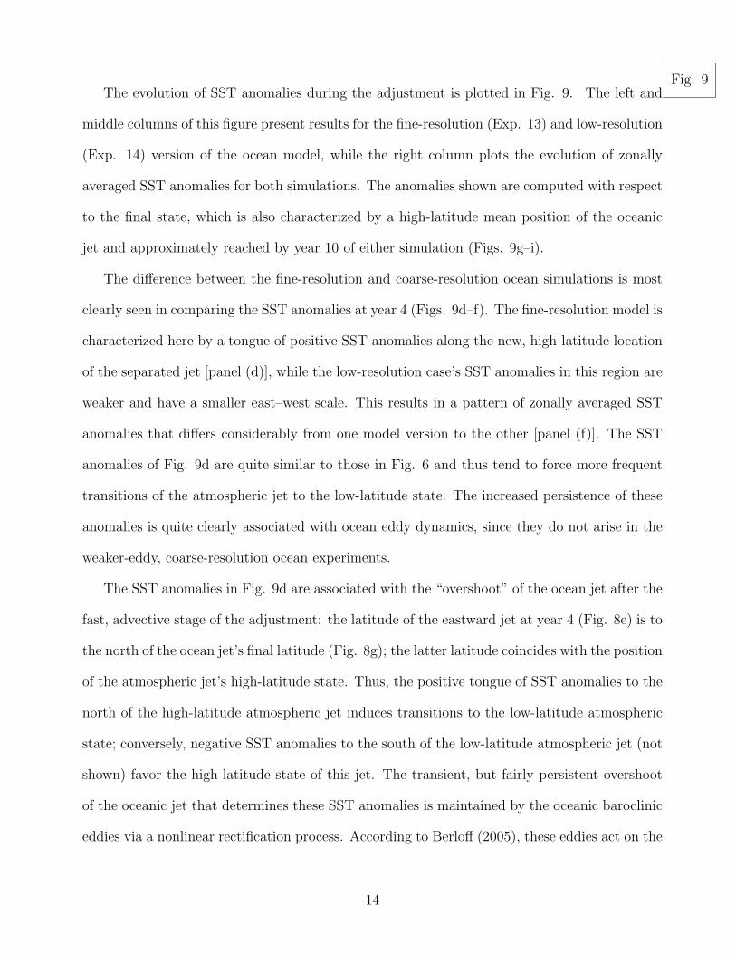
The evolution of SST anomalies during the adjustment is plotted in Fig. 9.Fig. 9

The left and

middle columns of this figure present results for the fine-resolution (Exp. 13) and low-resolution

(Exp. 14) version of the ocean model, while the right column plots the evolution of zonally

averaged SST anomalies for both simulations. The anomalies shown are computed with respect

to the final state, which is also characterized by a high-latitude mean position of the oceanic

jet and approximately reached by year 10 of either simulation (Figs. 9g–i).

The di!erence between the fine-resolution and coarse-resolution ocean simulations is most

clearly seen in comparing the SST anomalies at year 4 (Figs. 9d–f). The fine-resolution model is

characterized here by a tongue of positive SST anomalies along the new, high-latitude location

of the separated jet [panel (d)], while the low-resolution case’s SST anomalies in this region are

weaker and have a smaller east–west scale. This results in a pattern of zonally averaged SST

anomalies that di!ers considerably from one model version to the other [panel (f)]. The SST

anomalies of Fig. 9d are quite similar to those in Fig. 6 and thus tend to force more frequent

transitions of the atmospheric jet to the low-latitude state. The increased persistence of these

anomalies is quite clearly associated with ocean eddy dynamics, since they do not arise in the

weaker-eddy, coarse-resolution ocean experiments.

The SST anomalies in Fig. 9d are associated with the “overshoot” of the ocean jet after the

fast, advective stage of the adjustment: the latitude of the eastward jet at year 4 (Fig. 8e) is to

the north of the ocean jet’s final latitude (Fig. 8g); the latter latitude coincides with the position

of the atmospheric jet’s high-latitude state. Thus, the positive tongue of SST anomalies to the

north of the high-latitude atmospheric jet induces transitions to the low-latitude atmospheric

state; conversely, negative SST anomalies to the south of the low-latitude atmospheric jet (not

shown) favor the high-latitude state of this jet. The transient, but fairly persistent overshoot

of the oceanic jet that determines these SST anomalies is maintained by the oceanic baroclinic

eddies via a nonlinear rectification process. According to Berlo! (2005), these eddies act on the

14

large-scale oceanic flow as a small-scale stochastic forcing; this forcing, though, is organized by

the combined action of the nonlinearity and the "-e!ect so as to preferentially deposit positive

potential-vorticity anomalies to the north of the jet, and negative anomalies to the south. In

the coupled integrations using the coarse-resolution ocean model, the eddy field is weak, and

the eddy-driven stage of the adjustment is both shorter and less e!ective; consequently, the

coupled decadal mode is not found in these experiments.

We conclude, therefore, that ocean eddy dynamics is essential for the coupled oscillation in

setting up SST anomalies that are able to a!ect the atmospheric flow in a way that maintains

and reinforces the coupled mode. They are also instrumental in setting up the time scale of

the oscillation. The latter time scale is related to the duration of the eddy-driven adjustment

stage, which determines how long SST anomalies in the vicinity of the eastward jet can exist in

the absence of local atmospheric forcing; the resulting multi-year time lag leads to the decadal-

to-interdecadal oscillation. In order to further study the role of eddies in setting up the time

scale of the oscillation, we consider next experiments which use a lower ocean bottom drag

coe"cient, namely Exps. 7 and 15 of Table 1.

b. Coupled experiment with low ocean bottom drag

1) CLIMATOLOGY, SPECTRA, AND COMPOSITE CYCLE

The major di!erence between climatological patterns of ocean circulation from the coupled

run with low ocean bottom drag and their analog for the control run, which uses a larger value

for the bottom drag, is in the magnitude and spatial extent of the inertial recirculations. The

IR are stronger and occupy a larger area in the low-drag experiment (not shown). In this

regard, the results for the low-drag experiment are thus more realistic.

The spectrum of annually averaged data from Exp. 7 (not shown) exhibits a broad spectral

peak centered at about a 20-yr period, in both jet position and ocean kinetic energy time series.

15

The oceanic spectrum also exhibits a 5-yr peak representative of a coupled Rossby wave signal

(see section 5). The 20-yr oscillation has atmospheric and oceanic spatio-temporal patterns

(not shown) that resemble those of the 9-yr coupled oscillation discussed in Kravtsov et al.

(2006).

The composite cycle of the 20-yr oscillation in jet position and ocean kinetic energy (not

shown) is also very similar to that of the 9-yr oscillation of the control coupled run. In particular,

these two scalar quantities exhibit the same phase relations as the 9-yr coupled oscillation of

the control run (Fig. 5a): the jet position time series leads that of ocean kinetic energy by a

quarter of a cycle.

To summarize, the low-bottom-drag run thus exhibits the same type of oscillation as the

control run, but with a period that is roughly twice as long.

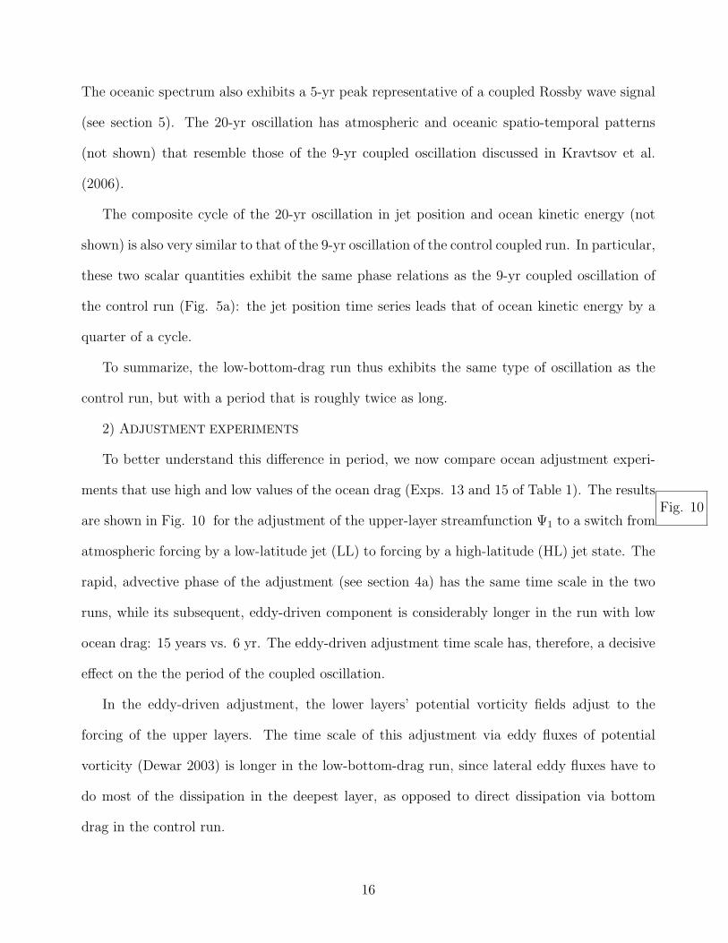
2) ADJUSTMENT EXPERIMENTS

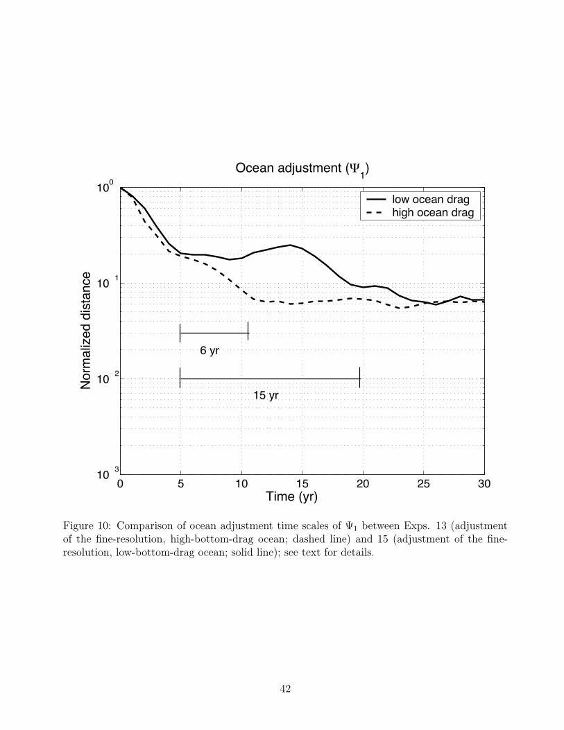
To better understand this di!erence in period, we now compare ocean adjustment experi-

ments that use high and low values of the ocean drag (Exps. 13 and 15 of Table 1). The results

are shown in Fig. 10Fig. 10

for the adjustment of the upper-layer streamfunction #1 to a switch from

atmospheric forcing by a low-latitude jet (LL) to forcing by a high-latitude (HL) jet state. The

rapid, advective phase of the adjustment (see section 4a) has the same time scale in the two

runs, while its subsequent, eddy-driven component is considerably longer in the run with low

ocean drag: 15 years vs. 6 yr. The eddy-driven adjustment time scale has, therefore, a decisive

e!ect on the the period of the coupled oscillation.

In the eddy-driven adjustment, the lower layers’ potential vorticity fields adjust to the

forcing of the upper layers. The time scale of this adjustment via eddy fluxes of potential

vorticity (Dewar 2003) is longer in the low-bottom-drag run, since lateral eddy fluxes have to

do most of the dissipation in the deepest layer, as opposed to direct dissipation via bottom

drag in the control run.

16

5 . Coupled Rossby wave mode

We now turn to the coupled Rossby wave mode, which is present in all the coupled experiments

(see Table 1) and has a period of 3–5 yr [see sections 3a and 4b(2)]. To visualize this mode,

we regress oceanic and atmospheric fields onto 1–10-yr band-pass filtered ocean kinetic energy

from Exp. 3, multiplied by #1 and normalized to have unit variance.

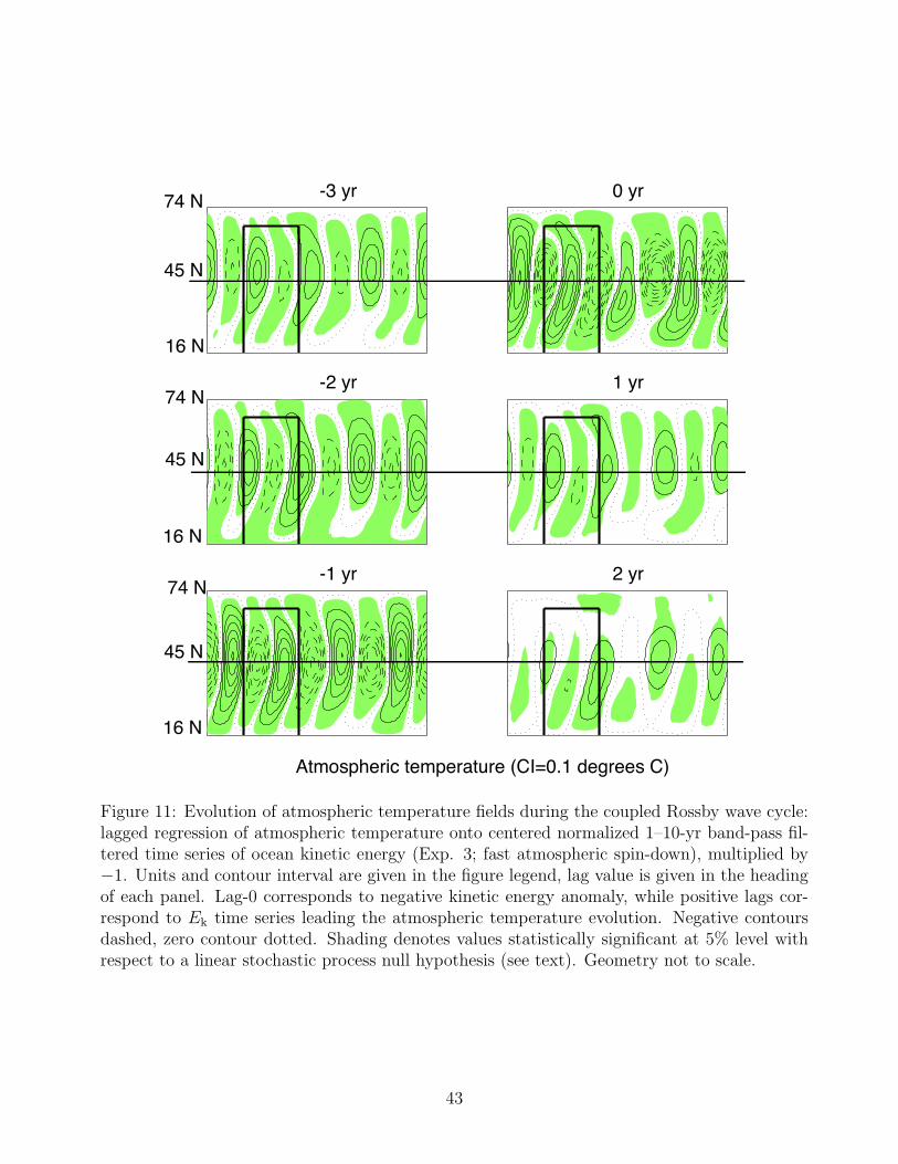
The results for atmospheric temperature are plotted in Fig. 11.Fig. 11

The evolution is charac-

terized by a westward-propagating wave-4. Circulation anomalies associated with this signal in

the upper ocean layer are shown in Fig. 12.Fig. 12

They have the same spatial scale as that of the

atmospheric wave (Fig. 11) and also propagate westward. SST evolution is depicted in Fig. 13.Fig. 13

Note that the SST wave is in phase with atmospheric temperature and in quadrature with #1.

Moreover, SSTs and atmospheric temperature anomalies have a similar magnitude, with SST

anomalies being slightly larger, which indicates that SST anomalies force atmospheric response

rather than vice versa.

It follows that this mode is a coupled Rossby wave of the type studied by Goodman and

Marshall (1999) in a linear channel model of both atmosphere and ocean. Our model has a

closed ocean basin, and the period of this linear oscillation is equal to the time it takes for

the lowest-mode Rossby wave of this basin to cross it (Sheremet et al. 1997; Chang et al.

2001). The dominant atmospheric wave associated with this Rossby basin mode is equivalent-

barotropic and its wavenumber 4 is also set by the ocean basin’s extent, which is equal to 1/4 of

the channel length. This wave does exist in uncoupled atmospheric experiments (Kravtsov et

al. 2005a), but exhibits no regularity in the interannual band. In the coupled integration, it is

amplified via a positive feedback with the ocean component’s Rossby basin mode, as described

by Goodman and Marshall (1999) in their channel model.

17

6 . Concluding remarks

a. Summary

This paper analyzes in greater detail a novel, highly nonlinear mechanism of coupled ocean–

atmosphere behavior in middle latitudes. This mechanism depends crucially on the nonlinear

dynamics of both fluids, namely (i) nonlinear sensitivity of atmospheric flow to ocean-induced

sea-surface temperature (SST) anomalies, which involves changes in the frequency of occurrence

of two distinct zonal-mean zonal flow regimes; and (ii) ocean eddy dynamics of the so-called

inertial recirculations (IRs), which enhance the SST anomalies that a!ect the atmosphere, as

well as determine the time scale of the coupled signal. The latter signal appears in the spectral

analysis of both the atmospheric and oceanic model time series as a broad peak in a decadal

range (Fig. 1). This peak is absent from all uncoupled integrations, as well as from fully coupled

integrations that use a coarser-resolution ocean model, with less eddy activity (see Table 1).

In section 3, we have discussed the role of atmospheric nonlinearity. The nature of atmo-

spheric behavior, that is bimodal vs. unimodal, depends on the value of the surface friction

coe"cient. The bimodality is present for intermediate and low values of the surface drag, while

the behavior at high drag is unimodal (see Kravtsov et al. 2005a and Fig. 2 of the present

paper). Coupled decadal oscillations appear only in the cases in which bimodality is present;

see Figs. 1b and 3b. The variance associated with this coupled oscillation decreases as one

tracks the model’s behavior to higher values of surface drag. The atmospheric signal in this

band appears as a decadal modulation of the transitions from the dominant, high-latitude jet

state to the much rarer low-latitude jet state.

At very low values of surface friction, however, while the bimodality is very pronounced

(Fig. 2a), the coupled signal is not found either (Fig. 3a), just like in the cases with high-drag,

unimodal behavior. This has to do with the transitions from the atmosphere’s preferred high-

18

latitude state to its low-latitude state becoming too infrequent, at a rate of about one transition

per decade, for low surface friction; in this case, the ocean cannot influence their occurrence

frequency on decadal time scales (Fig. 4).

We have chosen the westerly jet position to characterize the state of the atmosphere during

the coupled decadal-to-interdecadal cycle and the kinetic energy to characterize that of the

ocean. The composite decadal cycle of these two quantities, both of which are highly relevant

to the coupled variability, shows that the jet position leads ocean kinetic energy by a quarter

of a cycle (Fig. 5). Given a high-latitude jet, the ensuing high-energy state of the ocean is

associated with the development of an intense eastward jet, which penetrates far into the ocean

basin, and vigorous IRs. The resulting oceanic circulation anomalies cause SST anomalies (Fig.

6), which tend to induce more frequent transitions of the atmosphere to its low-latitude state.

These repeated transitions result in the collapse of the oceanic jet and development of SST

anomalies that favor the return of the atmosphere to its high-latitude state (Fig. 5b).

Section 4 provided evidence for the role of ocean eddy dynamics in the coupled oscillation.

In particular, we studied oceanic adjustment to a sudden switch in the atmospheric state

from a low-latitude to a high-latitude jet state, and vice versa, and we used three di!erent

models (Exps. 13–15 of Table 1): the fine-resolution ocean model of the control run, an ocean

model version that has a coarser resolution and hence a much weaker eddy activity, and a fine-

resolution ocean model version with a much smaller value of the ocean bottom drag coe"cient

than in the control run. In the coupled experiments that use these three models, only those

with the fine-resolution ocean exhibit a coupled oscillatory mode. The period of this mode is

roughly twice as long in the run with low ocean bottom drag, while it is entirely absent from

the runs with a coarse resolution ocean (Exps. 1, 4, and 7 of Table 1).

We found that the ocean’s adjustment to a predominantly high-latitude or low-latitude jet

forcing has two components: a fast, advective phase and a slower, eddy-dynamics-dominated

19

phase (Figs. 7–9). The duration of the former phase is of 3–5 years and depends relatively little

on the ocean bottom drag (Fig. 10), while the latter phase can more than double in length

(from 6 yr to 15 yr) as the bottom drag is reduced.

Higher resolution of the ocean model, and the resulting higher eddy activity, also give rise

to more persistent anomalies in the separated ocean jet region (Figs. 8, 9). The spatial pattern

of these anomalies produces heat-flux forcing on the atmosphere that favors atmospheric return

to the initial, pre-adjustment state (compare Figs. 9d and 6). We conclude, therefore, that IR

anomalies force the SST anomalies, which are able to e"ciently a!ect atmospheric transitions

between the two distinct regimes.

In addition to the nonlinear, 10–20-yr coupled mode described above, we have also found

a coupled mode that depends neither on atmospheric bimodality, nor on the ocean’s eddy

dynamics. This interannual, linear coupled Rossby mode has been discussed in section 5.

Phase relations between the oceanic and atmospheric fields (Figs. 11–13) show that this mode

is analogous to the one studied by Goodman and Marshall (1999) in a channel geometry. Given

our model’s closed ocean basin, the time scale of this oscillation appears to be set by the time

it takes to the oceanic Rossby wave to cross the basin.

We have argued that ocean eddies contribute substantially to SST anomalies that play

a key role in the coupled oscillation, as well as to the oceanic adjustment time scale and,

therewith, to the oscillation’s period. We have done so in the present paper only by comparing

the results of di!erent coupled and uncoupled integrations. In order to understand in greater

depth and detail the way ocean eddies operate in the coupled context, we have developed a

novel technique to parameterize ocean eddies stochastically in a coupled model that uses a

coarser resolution ocean. We have shown, in particular, that the coupled behavior absent from

a model that uses a coarse-resolution ocean component is recovered when our novel stochastic

20

eddy parameterization is applied (Berlo! et al. 2006).

b. Discussion

Our model is highly idealized (low vertical resolution, quasi-geostrophic dynamics, idealized

geography, simplistic parameterizations of heat and momentum exchange between the ocean

and the atmosphere etc.) and therefore its results (likewise, the results from any type of an

idealized model or theory) must be treated with caution when relating them to the real world.

Having said that, we will now argue for a broad correspondence between patterns and time

scales of variability we have modeled and the observed ones.

The highly nonlinear coupled mode discussed here does not arise from an intrinsic oceanic

mode: it involves, instead, a coupled adjustment process, in which the ocean modifies intrinsic

atmospheric variability on decadal-to-interdecadal time scales via a nonlinear feedback due

to interaction between the ocean’s large-scale flow and turbulent eddies. The most realistic

results, in terms of the spatial extent and strength of the oceanic inertial recirculations, were

obtained for low values of the oceanic bottom drag. For the optimal values of the bottom

drag and resolution in the ocean model, the period of our nonlinear coupled mode is of about

15–25 yr, rather than the 9–10 yr for the control run. This interdecadal band has been found

to be prominent in climatic signals over the North Atlantic (Plaut et al. 1995; Moron et al.

1998), as well as over the North Pacific (Chao et al. 2000) and in global SSTs and surface air

temperatures (Folland et al. 1984; Ghil and Vautard 1991).

An interannual mode of intrinsic oceanic variability, called the gyre mode, has been discov-

ered and well documented in a hierarchy of increasingly realistic ocean-only models (Jiang et

al. 1995; Speich et al. 1995; Ghil et al. 2002b; Simonnet et al. 2003a,b, 2006; Dijkstra and Ghil

2006). The gyre mode’s fundamental period depends mainly on the nonlinear dynamics of the

recirculation dipole near the separation of western boundary currents and is fairly independent

of basin size. This period lies in the 5–10-yr band and seems to provide a plausible explana-

21

tion for the 7–8-yr peak in North Atlantic SSTs (Moron et al. 1998), and sea-level pressure

(Da Costa and Colin de Verdiere 2002), as well as in the meridional displacements of the Gulf

Stream axis (Dijkstra and Ghil 2006; Simonnet et al. 2006), the North Atlantic Oscillation

index (Wunsch 1999), and the 335-yr-long time series of Central England temperatures (Plaut

et al. 1995).

The spatial patterns of this mode bear certain similarities to those of our highly nonlinear

coupled variability: they both involve modulations of the oceanic eastward jet’s meridional

position, intensity, and eastward penetration into the basin, as well as associated reorganizations

of the IR region. Still, Moron et al. (1998) show substantial di!erences between the basin-wide

SST patterns of the 13–14-yr mode (their Fig. 9) and the 7–8-yr mode (their Fig. 10) in

the North Atlantic, although both have particularly strong anomalies along the East Coase of

North America, between the Florida Straits and the Great Banks. There is a good likelihood,

therefore, that the present, 15–25-yr coupled mode might contribute to the interdecadal climate

variability documented not only in the North Atlantic (Deser and Blackmon 1993; Kushnir 1994;

Moron et al. 1998), but also in the North Pacific (Mantua et al. 1997; Chao et al. 2000) and

globally (Folland et al. 1984; Ghil and Vautard 1991).

This being said, it appears fortunate that our coupled model does not support the gyre mode;

indeed, this fact allowed us to identify and study in some depth the novel, highly nonlinear,

truly coupled mode, with its 15–25-yr period, described in the present study. The reasons

behind the absence of the gyre mode in our ocean model require further investigation.

To make matters even more complicated and interesting, Hogg et al. (2005a,b) have obtained

a 15-yr oscillation in a coupled model similar to ours, but in which atmospheric behavior is

not bimodal. Their oscillatory mode seems to be driven by intrinsic oceanic variability, whose

spatial patterns resemble the gyre mode. In the work of Hogg et al. (2005a,b), like in that

of Feliks et al. (2004; see also Y. Feliks, M. Ghil, and E. Simonnet, pers. commun., 2005),

22

the intrinsic oceanic variability modulates the intrinsic modes of atmospheric variability on

interdecadal or interannual time scales, respectively. Simonnet (2006) has shown that the gyre

mode, in the presence of bottom friction, can be “quantized,” according to basin size, that is

it can exhibit harmonics depending on the number of eastward-jet meanders accomodated by

the basin. It is possible, therefore, to have gyre modes with both 7–8-yr and 15-yr periods.

We are thus faced with an embarassment of riches: two or three di!erent sources of mid-

latitude climate variability, either ocean-driven or truly coupled. To distinguish between these

types of mid-latitude climate variability in observations and general circulation model simu-

lations is not that easy, since the spatial patterns, dynamical mechanisms, and time scales of

the associated modes bear certain similarities. A possible direction to follow in this regard is

to look for the statistical signatures of ocean–atmosphere co-variability that will di!er from

one mode to another. Such statistical studies will have to be complemented by a better un-

derstanding of the way the modes di!er dynamically from each other. Provided statistical and

dynamical insights that uniquely identify each of the modes are available, it will be possible

to make inferences about which of the modes, or combinations thereof, contribute (if at all) to

which frequency band of climate variability.

Acknowledgements. It is a pleasure to thank D. Kondrashov and A. W. Robertson for helpful

discussions. The comments of anonymous reviewers have helped to improve the presentation.

This research was supported by NSF grant OCE-02-221066 (all co-authors) and DOE grant

DE-FG-03-01ER63260 (MG and SK).

23

References

Allen, R. M., and L. A. Smith, 1996: Monte Carlo SSA: Detecting irregular oscillations in the

presence of colored noise. J. Climate, 9, 3373–3404.

Berlo!, P., 2005: On rectification of randomly forced flows. J. Mar. Res., 31, 497–527.

Berlo!, P., W. K. Dewar, S. Kravtsov, and J. C. McWilliams, 2006: Ocean eddy dynamics in

a coupled ocean–atmosphere model. J. Phys. Oceanogr., sub judice.

Chang, K.-I., M. Ghil, K. Ide, and C.-C. A. Lai, 2001: Transition to aperiodic variability in a

wind-driven double-gyre circulation model. J. Phys. Oceanogr., 31, 1260–1286.

Chao, Y., M. Ghil, and J. C. McWilliams, 2000: Pacific interdecadal variability in this century’s

sea surface temperatures. Geophys. Res. Lett., 27, 2261-2264.

Da Costa, E. D., and A. C. de Verdiere, 2002: The 7.7-year North Atlantic oscillation. Q. J.

R. Meteorol. Soc., 128A, 797–817.

Deser, C., and M. L. Blackmon, 1993: Surface climate variations over the North Atlantic Ocean

during winter: 1900-1989. J. Climate, 6, 1743–1753.

Dettinger, M. D., M. Ghil, C. M. Strong, W. Weibel, and P. Yiou, 1995: Software expedites

singular-spectrum analysis of noisy time series. Eos, Trans. AGU, 76, pp. 12, 14, 21.

Dewar, W. K., 2003: Nonlinear midlatitude ocean adjustment. J. Phys. Oceanogr., 33, 1057–

1081.

Dijkstra, H. A., and M. Ghil, 2006: Low-frequency variability of the large-scale ocean circula-

tion: A dynamical systems approach. Rev. Geophys., in press.

24

Folland, C. K., D. E. Parker, and F. E. Kates, 1984: Worldwide marine temperature fluctuations

1856–1981. Nature, 310, 670–673.

Ghil, M., and K. C. Mo, 1991: Intraseasonal oscillations in the global atmosphere. Part I:

Northern Hemisphere and tropics. J. Atmos. Sci., 48, 752–779.

Ghil, M., and R. Vautard, 1991: Interdecadal oscillations and the warming trend in global

temperature time series. Nature, 350, 324–327.

Ghil, M., M. R. Allen, M. D. Dettinger, K. Ide, D. Kondrashov, M. E. Mann, A. W. Robertson,

A. Saunders, Y. Tian, F. Varadi, and P. Yiou, 2002a: Advanced spectral methods for

climatic time series. Rev. Geophys., 40, 3-1–3-41, 10.1029/2000GR000092.

Ghil, M., Y. Feliks, and L. Sushama, 2002b: Baroclinic and barotropic aspects of the wind-

driven ocean circulation. Physica D, 167, 1–35.

Goodman, J., and J. Marshall, 1999: A model of decadal middle-latitude atmosphere–ocean

interaction. J. Climate, 12, 621–641.

Hogg, A. M., P. D. Killworth, J. R. Blundell, and W. K. Dewar, 2005a: Mechanisms of decadal

variability of the wind-driven ocean circulation. J. Phys. Oceanogr., 35, 512–531.

Hogg, A. M., W. K. Dewar, P. D. Killworth, and J. R. Blundell, 2005b: Decadal variability of

the midlatitude climate system driven by the ocean circulation. J. Climate, in press.

Jiang, S., F.-F. Jin, and M. Ghil, 1995: Multiple equilibria, periodic and aperiodic solutions in

a wind-driven, double-gyre, shallow-water model. J. Phys. Oceanogr., 25, 764–786.

Keppenne, C. L., and M. Ghil, 1993: Adaptive filtering and prediction of noisy multivariate

signals: An application to subannual variability in atmospheric angular momentum. Intl.

J. Bifurcation & Chaos, 3, 625–634.

25

Kravtsov, S., and A. W. Robertson, 2002: Midlatitude ocean–atmosphere interaction in an

idealized coupled model. Climate Dyn., 19, 693–711.

Kravtsov, S., A. W. Robertson, and M. Ghil, 2005a: Bimodal behavior in a baroclinic "-channel

model. J. Atmos. Sci., 62, 1746–1769.

Kravtsov, S., D. Kondrashov, and M. Ghil, 2005b: Multiple regression modeling of nonlinear

processes: Derivation and applications to climatic variability. J. Climate, 18, 4404–4424.

Kravtsov, S., W. K. Dewar, P. Berlo!, J. C. McWilliams, and M. Ghil, 2006: A highly nonlin-

ear coupled mode of decadal variability in a mid-latitude ocean–atmosphere model. Dyn.

Atmos. Oceans, submitted. Available from www.atmos.ucla.edu/tcd.

Kushnir, Y., and I. Held, 1996: Equilibrium atmospheric response to North Atlantic SST

anomalies. J. Climate, 9, 1208–1220.

Mann, M. E., and J. M. Lees, 1996: Robust estimation of background noise and signal detection

in climatic time series. Clim. Change, 33, 409–445.

Mantua, N. J., S. R. Hare, Y. Zhang, J. M. Wallace, and R. C. Francis, 1997: A Pacific

interdecadal climate oscillation with impacts on salmon production. Bull. Amer. Meteor.

Soc., 78, 1069–1079.

Mehta, V. M., M. J. Suarez, J. V. Manganello, and T. L. Delworth, 2000: Oceanic influence

on the North Atlantic Oscillation and associated Northern Hemisphere climate variations:

1959–1993. Geoph. Res. Letts., 27, 121–124.

Moron, V., R. Vautard, and M. Ghil, 1998: Trends, interdecadal and interannual oscillations

in global sea-surface temperatures. Clim. Dyn., 14, 545–569.

Plaut, G., and R. Vautard, 1994: Spells of low-frequency variability and weather regimes in

the Northern Hemisphere. J. Atmos. Sci., 51, 210–236.

26

Plaut, G., M. Ghil, and R. Vautard, 1995: Interannual and interdecadal variability in 335 years

of Central England temperatures. Science, 268, 710–713.

Preisendorfer, R. W., 1988: Principal Component Analysis in Meteorology and Oceanography.

Elsevier, New York, pp. 425.

Rodwell, M. J., D. P. Rodwell, and C. K. Folland, 1999: Oceanic forcing of the wintertime

North Atlantic Oscillation and European climate. Nature, 398, 320–323.

Saravanan, R., 1998: Atmospheric low-frequency variability and its relationship to midlatitude

SST variability: Studies using NCAR Climate System Model. J. Climate, 11, 1386–1404.

Sheremet, V. A., G. R. Ierley, and V. M. Kamenkovich, 1997: Eigenanalysis of the two-

dimensional wind-driven ocean circulation problem. J. Mar. Res., 55, 57–92.

Simonnet, E., 2006: Quantization of the low-frequency variability of the double-gyre circulation.

J. Phys. Oceanogr., in press.

Simonnet, E., M. Ghil, K. Ide, R. Temam, and S. Wang, 2003a: Low-frequency variability in

shallow-water models of the wind-driven ocean circulation. Part I: Steady-state solutions.

J. Phys. Oceanogr., 33, 712–728.

Simonnet, E., M. Ghil, K. Ide, R. Temam, and S. Wang, 2003b: Low-frequency variability

in shallow-water models of the wind-driven ocean circulation. Part II: Time-dependent

solutions. J. Phys. Oceanogr., 33, 729–752.

Simonnet, E., M. Ghil, and H. A. Dijkstra, 2006: Homoclinic bifurcations in the quasi-

geostrophic double-gyre circulation. J. Mar. Res., in press.

Speich, S., H. Dijkstra, and M. Ghil, 1995: Successive bifurcations in a shallow-water model,

applied to the wind-driven ocean circulation. Nonlin. Proc. Geophys., 2, 241–268.

27

Thomson, D. J., 1982: Spectrum estimation and harmonic analysis. IEEE Proc., 70, 1055–1096.

Thomson, D. J., 1990: Quadratic-inverse spectrum estimates: Application to paleoclimatology.

Philos. Trans. R. Soc. London, A332, 539–597.

Vautard, R., and M. Ghil, 1989: Singular spectrum analysis in nonlinear dynamics, with ap-

plications to paleoclimatic time series. Physica D, 35, 395–424.

Vautard, R., P. Yiou, and M. Ghil, 1992: Singular-spectrum analysis: A toolkit for short, noisy

chaotic signals. Physica D, 58, 95–126.

Wunsch, C., 1999: The interpretation of short climate records, with comments on the North

Atlantic and Southern Oscillations. Bull. Amer. Meteorol. Soc., 80, 245–255.

28

Table Captions

TABLE 1. Summary of experiments. Columns show: number of an experiment; duration

of experiment (yr); atmospheric barotropic spin-down time scale k!1 (days); resolution of the

ocean model (km); ocean horizontal viscosity AH (m2 s!1); equivalent depth of the ocean bottom

Ekman layer Df (m); type of forcing; presence of bimodality in the atmospheric circulation;

degree of atmospheric intermittency (average number of transition events from high-latitude to

low-latitude jet states per year); presence of nonlinear coupled mode and its period (yr); and

presence of a 3–5-yr linear coupled Rossby wave mode. Last column provides comments on a

given experiment. Dashes indicate repetition of entry within a given column; N/A stands for

“not applicable.”

29

Figure Captions

Fig. 1. Multi-taper method (MTM) spectra of ocean kinetic energy: control run (Exp. 1).

Fig. 2. Probability density function (PDF) of atmospheric jet position: (a) Exp. 2 of Table

1 (slow spin-down); and (b) Exp. 3 of Table 1 (fast spin-down).

Fig. 3. Multi-taper method (MTM) spectra of ocean kinetic energy: (a) Exp. 2 (slow

spin-down); and (b) Exp. 3 (fast spin-down).

Fig. 4. Jet-position time series (40-day averages): (a) Exp. 2 (slow spin-down); (b) Exp. 1

(control run of Part I; intermediate spin-down); and (c) Exp. 3 (fast spin-down).

Fig. 5. Composites of characteristic features of the model, keyed to eight phase categories of

the 9-yr coupled oscillation of Exp. 1 (control run of Part I; intermediate spin-down): (a) ocean

kinetic energy and atmospheric jet position in the control run; and (b) conditional probability

of the low-latitude jet position, given prescribed ocean states corresponding to the oscillation’s

phase categories (Exp. 12).

Fig. 6. Di!erence between composite SSTs from phases 5 and 1 of Exp. 12 (see Fig. 5b).

Contour interval is 0.5 deg C, negative contours dashed, zero contours dotted.

Fig. 7. Ocean adjustment experiments (Exps. 13 and 14). Shown are rms distances from

the final high-latitude-jet-forced ocean state (HL), normalized by the distance between this

latter state and the initial one, which is forced by the low-latitude jet (LL): Exp. 13 (fine-

resolution ocean; solid line) and Exp. 14 (coarse-resolution ocean; dashed line). The distances

shown are measured between the corresponding zonally averaged SST fields; see text for details.

Fig. 8. Snapshots of the upper-layer streamfunction #1 for the ocean adjustment experi-

ments of Fig. 7: left column – Exp. 13 (adjustment of the fine-resolution ocean); right column –

Exp. 14 (adjustment of the coarse-resolution ocean). (a,b) Initial (unfiltered) state; (c,d) state

after 2 yr; (e,f) after 4 yr; and (g,h) after 10 yr. Contour interval is 5 Sv; negative contours

30

dashed.

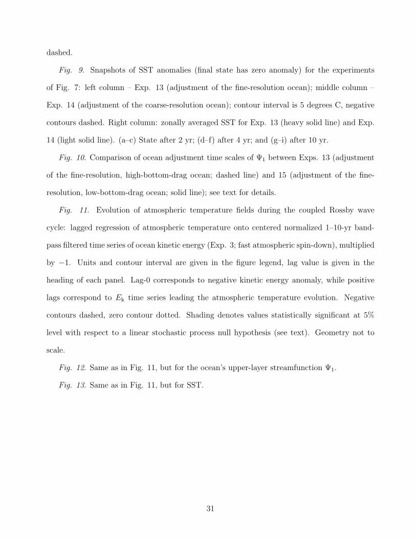
Fig. 9. Snapshots of SST anomalies (final state has zero anomaly) for the experiments

of Fig. 7: left column – Exp. 13 (adjustment of the fine-resolution ocean); middle column –

Exp. 14 (adjustment of the coarse-resolution ocean); contour interval is 5 degrees C, negative

contours dashed. Right column: zonally averaged SST for Exp. 13 (heavy solid line) and Exp.

14 (light solid line). (a–c) State after 2 yr; (d–f) after 4 yr; and (g–i) after 10 yr.

Fig. 10. Comparison of ocean adjustment time scales of #1 between Exps. 13 (adjustment

of the fine-resolution, high-bottom-drag ocean; dashed line) and 15 (adjustment of the fine-

resolution, low-bottom-drag ocean; solid line); see text for details.

Fig. 11. Evolution of atmospheric temperature fields during the coupled Rossby wave

cycle: lagged regression of atmospheric temperature onto centered normalized 1–10-yr band-

pass filtered time series of ocean kinetic energy (Exp. 3; fast atmospheric spin-down), multiplied

by #1. Units and contour interval are given in the figure legend, lag value is given in the

heading of each panel. Lag-0 corresponds to negative kinetic energy anomaly, while positive

lags correspond to Ek time series leading the atmospheric temperature evolution. Negative

contours dashed, zero contour dotted. Shading denotes values statistically significant at 5%

level with respect to a linear stochastic process null hypothesis (see text). Geometry not to

scale.

Fig. 12. Same as in Fig. 11, but for the ocean’s upper-layer streamfunction #1.

Fig. 13. Same as in Fig. 11, but for SST.

31

TA

BL

E 1

. Su

mm

ary o

f exp

erimen

ts. Co

lum

ns sh

ow

: nu

mb

er of an

exp

erim

ent; d

uratio

n o

f exp

erimen

t (yr); a

tmo

sph

eric baro

trop

ic spin

-do

wn

time scale

k-1 (d

ays); reso

lutio

n o

f the o

cean m

od

el (km

); ocean

ho

rizon

tal visco

sity A

H (m2

s-1); eq

uiv

alent d

epth

of th

e ocean

bo

ttom

Ek

man

layer

Df ; ty

pe o

f forcin

g; p

resence o

f bim

od

ality in

the atm

osp

heric circu

lation

; deg

ree o

f atmo

sph

eric in

termitten

cy (av

erage n

um

ber o

f transitio

n

even

ts from

hig

h-latitu

de to

low

-latitud

e jet states per y

ear); presen

ce o

f no

nlin

ear cou

pled

mo

de an

d its p

eriod

(yr); an

d p

resence

of a 3

–5

-yr

linear co

up

led R

ossb

y w

ave m

od

e. Last co

lum

n p

rov

ides co

mm

ents o

n a

giv

en ex

perim

ent. D

ashes in

dicate re

petitio

n o

f entry

with

in a g

iven

colu

mn

; N/A

stand

s for ``n

ot ap

plicab

le."

Exp.

Dur.

k-1

R

es. AH

Df

Forcin

g

Bim

. In

termit.

NL

R

N

otes

(1)

1000

6.1

7

10

200

30

Coupled

yes

1–2

5–15

yes

Contro

l run

(2)

800

7.1

2

—

—

—

—

—

0.1

–0.2

no

—

(3)

400

5.4

5

—

—

—

—

weak

10–20

5–15

—

(4)

800

6.1

7

20

1000

—

—

yes

1–2

no

—

(5)

—

7.1

2

—

—

—

—

—

0.1

–0.2

—

—

(6)

—

5.4

5

—

—

—

—

weak

10–20

—

—

(7)

—

6.1

7

10

200

3

—

yes

1–2

15–25

—

Low

ocean

drag

(8)

400

N/A

—

—

30

Atm

. stoch

. (1)

N/A

N

/A

no

no

Ocean

-only

run

(9)

1000

6.1

7

40

N/A

N

/A

Oce. clim

. (1)

yes

1–2

—

—

Atm

osp

here+

mix

ed lay

er run

(10)

800

7.1

2

—

—

—

Oce. clim

. (2)

—

0.1

–0.2

—

—

—

(11)

—

5.4

5

—

—

—

Oce. clim

. (3)

weak

10–20

—

—

—

(12)

800x8

6.1

7

—

—

—

Oce.

com

posites (1

)

yes

1–2

N/A

N

/A

Show

s that o

cean affects atm

osp

here

(13)

100x3

N/A

10

200

30

Atm

.

com

posites (2

)

N/A

N

/A

N/A

N

/A

Fin

e-resolu

tion o

cean ad

justm

ent

(14)

—

—

20

1000

—

Atm

.

com

posites (5

)

—

—

—

—

Coarse-reso

lutio

n o

cean ad

justm

ent:

differen

t pattern

/time d

epen

den

ce

(15)

—

—

10

200

3

Atm

.

com

posites (7

)

—

—

—

—

Adju

stmen

t in th

e ocean

model u

sing

low

botto

m d

rag: p

atterns are sim

ilar

to (1

3), b

ut tim

e scale is longer

32

0 0.05 0.1 0.15 0.2 0.25 0.3 0.35 0.4 0.45 0.5100

101

102

103Ocean kinetic energy MTM spectrum

Frequency (yr!1)

Spe

ctra

l den

sity

raw95%99%9 yr 5 yr

Figure 1: Multi-taper method (MTM) spectra of ocean kinetic energy: control run (Exp. 1).

33

35 40 45 50 55 600

0.05

0.1

0.15

0.2

0.25

0.3

0.35Jet!position PDF

Latitude (deg. N)

Pro

babi

lity

dens

ity

(a)35 40 45 50 55 60

0

0.05

0.1

0.15

0.2

0.25

0.3

0.35Jet−position PDF

Latitude (deg. N)(b)

Figure 2: Probability density function (PDF) of atmospheric jet position: (a) Exp. 2 of Table1 (slow spin-down); and (b) Exp. 3 of Table 1 (fast spin-down).

34

0 0.05 0.1 0.15 0.2 0.25 0.3 0.35 0.4 0.45 0.510

0

101

102

103

Ocean kinetic energy MTM spectrumS

pe

ctra

l de

nsi

ty(a)

raw99%95%

0 0.05 0.1 0.15 0.2 0.25 0.3 0.35 0.4 0.45 0.510

0

101

102

103

Sp

ect

ral d

en

sity

Frequency (yr-1 )

(b)

raw99%95%

4 yr

10 yr 4 yr

Figure 3: Multi-taper method (MTM) spectra of ocean kinetic energy: (a) Exp. 2 (slow spin-down); and (b) Exp. 3 (fast spin-down).

35

0 50 100 150 20035

40

45

50

55

60Jet position

Latit

ude

(deg

N)

(a)

0 50 100 150 20035

40

45

50

55

60

Latit

ude

(deg

N)

(b)

0 50 100 150 20035

40

45

50

55

Latit

ude

(deg

N)

Time (yr)

(c)

Figure 4: Jet-position time series (40-day averages): (a) Exp. 2 (slow spin-down); (b) Exp. 1(control run of Part I; intermediate spin-down); and (c) Exp. 3 (fast spin-down).

36

1 2 3 4 5 6 7 8!2

!1.5

!1

!0.5

0

0.5

1

1.5N

orm

aliz

ed q

uant

ityComposite

ocean kinetic energyjet position

1 2 3 4 5 6 7 8

0.126

0.128

0.13

0.132

0.134

0.136

0.138

0.14Probability of the jet being in low!latitude state

Phase category of the 9!yr oscillation

Frac

tion

of d

ays

spen

t in

low!l

atitu

de s

tate

(a)

(b)

Figure 5: Composites of characteristic features of the model, keyed to eight phase categories ofthe 9-yr coupled oscillation of Exp. 1 (control run of Part I; intermediate spin-down): (a) oceankinetic energy and atmospheric jet position in the control run; and (b) conditional probabilityof the low-latitude jet position, given prescribed ocean states corresponding to the oscillation’sphase categories (Exp. 12). 37

X

Y

SST difference between phases 5 and 1

45 N

16 N

66 N

0 km 5120 km

Figure 6: Di!erence between composite SSTs from phases 5 and 1 of Exp. 12 (see Fig. 5b).Contour interval is 0.5 deg C, negative contours dashed, zero contours dotted.

38

0 5 10 15 20 25 300

0.1

0.2

0.3

0.4

0.5

0.6

0.7

0.8

0.9

Transition from LL to HL state

Time (yr)

No

rma

lize

d d

ista

nce

high-resolution ocean

low-resolution ocean

3 yr

6 yr

Figure 7: Ocean adjustment experiments (Exps. 13 and 14). Shown are rms distances from thefinal high-latitude-jet-forced ocean state (HL), normalized by the distance between this latterstate and the initial one, which is forced by the low-latitude jet (LL): Exp. 13 (fine-resolutionocean; solid line) and Exp. 14 (coarse-resolution ocean; dashed line). The distances shown aremeasured between the corresponding zonally averaged SST fields; see text for details.

39

16 N

45 N

66 N

66 N

66 N

66 N

16 N

16 N

16 N

45 N

45 N

45 N

Figure 8: Snapshots of the upper-layer streamfunction #1 for the ocean adjustment experimentsof Fig. 7: left column – Exp. 13 (adjustment of the fine-resolution ocean); right column – Exp.14 (adjustment of the coarse-resolution ocean). (a,b) Initial (unfiltered) state; (c,d) state after2 yr; (e,f) after 4 yr; and (g,h) after 10 yr. Contour interval is 5 Sv; negative contours dashed.

40

16 N

45 N

66 N

66 N

66 N

16 N

16 N

45 N

45 N

Figure 9: Snapshots of SST anomalies (final state has zero anomaly) for the experiments of Fig.7: left column – Exp. 13 (adjustment of the fine-resolution ocean); middle column – Exp. 14(adjustment of the coarse-resolution ocean); contour interval is 5 degrees C, negative contoursdashed. Right column: zonally averaged SST for Exp. 13 (heavy solid line) and Exp. 14 (lightsolid line). (a–c) State after 2 yr; (d–f) after 4 yr; and (g–i) after 10 yr.

41

0 5 10 15 20 25 3010

3

10 2

10 1

100

Ocean adjustment (Ψ1)

Time (yr)

No

rma

lize

d d

ista

nce

low ocean draghigh ocean drag

6 yr

15 yr

Figure 10: Comparison of ocean adjustment time scales of #1 between Exps. 13 (adjustmentof the fine-resolution, high-bottom-drag ocean; dashed line) and 15 (adjustment of the fine-resolution, low-bottom-drag ocean; solid line); see text for details.

42

-3 yr

-2 yr

-1 yr

0 yr

1 yr

2 yr

Atmospheric temperature (CI=0.1 degrees C)

45 N

74 N

16 N

16 N

16 N

45 N

45 N

74 N

74 N

Figure 11: Evolution of atmospheric temperature fields during the coupled Rossby wave cycle:lagged regression of atmospheric temperature onto centered normalized 1–10-yr band-pass fil-tered time series of ocean kinetic energy (Exp. 3; fast atmospheric spin-down), multiplied by#1. Units and contour interval are given in the figure legend, lag value is given in the headingof each panel. Lag-0 corresponds to negative kinetic energy anomaly, while positive lags cor-respond to Ek time series leading the atmospheric temperature evolution. Negative contoursdashed, zero contour dotted. Shading denotes values statistically significant at 5% level withrespect to a linear stochastic process null hypothesis (see text). Geometry not to scale.

43

-3 yr -2 yr -1 yr

0 yr 1 yr 2 yr

Ψ1 (CI=1.2 Sv)

16 N

66 N

45 N

45 N

16 N

66 N

Figure 12: Same as in Fig. 11, but for the ocean’s upper-layer streamfunction #1.

44

-3 yr -2 yr -1 yr

0 yr 1 yr 2 yr

SST (CI=0.1 degrees C)

16 N

45 N

66 N

66 N

16 N

45 N

Figure 13: Same as in Fig. 11, but for SST.

45