dye tracer studies in the pacific northwest - pncwa

DDYEYE TTRACERRACER SSTUDIESTUDIES

David McBride, PE and Bill Fox, PECosmopolitan Engineering Group

PNCWA ConferenceBend, Oregon

October 26, 2010

Tracer Study ObjectivesTracer Study Objectives

• Outfall inspections (Integrity/Function)

• Quantify dilution

• Quantify reflux

• Calibrate hydrodynamic model

• Calculate residual circulation/flushing time

• Measure dispersion coefficients

• Transport to critical areas

• Discharge measurement

Outfall InspectionsOutfall Inspections

Quantify Dilution Quantify Dilution –– OverviewOverview

• Tracers

• Equipment

• Injection

• Plume Measurement Methods

• Ancillary data

• Interpretation

Fluorescent TracersFluorescent Tracers

• What is a fluorescent substance?• The ideal tracer

– Water soluble– Strongly fluorescent– Unique spectrum– Stable– Harmless– Inexpensive

• Fluorescent tracers– Rhodamine WT - Pontacyl Pink– Rhodamine B - Chlorophyll– Fluorescein - Hydrocarbons

Rhodamine WTRhodamine WT

• Red, fluorescent dye

• Stable in the environment

• Non-toxic

• Highly visible

• Shipped in 24% solution (s.g. = 1.15)

• Approximately $25/lb

• Keystone Aniline (Compton, CA)


• Concentration comparison

Dye Concentration(ppb) Commentary

1.0 Low end of desired detection range10 Visible in clear reservoir

25-50 Calibration reference standard100 Near upper limit of linear range

10,000 Non-toxic to aquatic life238 million 23.8% stock solution Rhodamine WT


• Factors affecting fluorescence– Temperature

– Reactivity (Cl2, SO2, O2)

– Photochemical decay

– Sorption

– Concentration quenching

Turbidity Effect on FluorescenceTurbidity Effect on Fluorescence

Alternate Tracers Alternate Tracers –– ConductivityConductivity

Alternate Tracers Alternate Tracers –– TemperatureTemperature

Alternate Tracers Alternate Tracers –– SeleniumSelenium

Equipment Equipment -- FluorometersFluorometers

• Turner Model 10-AU

• Lab Fluorometers

• Turner SCUFA

• Field Models

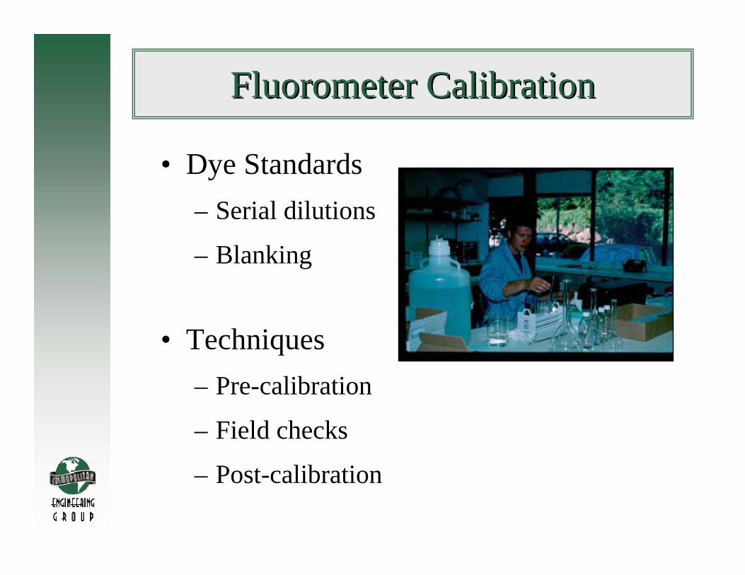
Fluorometer CalibrationFluorometer Calibration

• Dye Standards– Serial dilutions

– Blanking

• Techniques– Pre-calibration

– Field checks

– Post-calibration

Fluorometer CalibrationFluorometer Calibration

Dye InjectionDye Injection

• Goal: Uniform concentration

• Pumping setup

• Target concentration (500-5,000 ppb)

• Dye monitoring

• Manhole sampling

Dye Injection EquipmentDye Injection Equipment

• Peristaltic Pump

Dye InjectionDye Injection

Field Methods Field Methods –– Shallow StreamShallow Stream

• Wade• Ropes/range lines for positioning• Discrete samples to laboratory

Field Methods Field Methods –– Visible PlumeVisible Plume

• Submersible (SCUFA)

• Flow-through (Turner 10-AU)

• Position with ropes and anchors

• GPS recordings/rope stationing

• Link to CTD for depth

Field Methods Field Methods –– Visible PlumeVisible Plume

Field Methods Field Methods –– Submerged PlumeSubmerged Plume

• Boat

• Plume reconnaissance

• Position with ropes, anchors, GPS coordinates, CTD

• Density stratified?

• Use drogues

Field Methods Field Methods –– Vessel PositioningVessel Positioning

Ancillary MeasurementsAncillary Measurements

Ancillary Data Ancillary Data –– Current MeterCurrent Meter

Ancillary Data Ancillary Data –– CTD ProfilesCTD Profiles

Plume Measurements Plume Measurements –– Bottle SamplesBottle Samples

Plume Measurements Plume Measurements –– TransectsTransects

Plume Measurements Plume Measurements –– ProfilesProfiles

Plume Measurements Plume Measurements –– Time SeriesTime Series

Plume Measurements Plume Measurements –– ShotgunShotgun

Plume Measurements Plume Measurements –– SawtoothSawtooth

Density StratificationDensity Stratification

Farfield Plume TransectsFarfield Plume Transects

Farfield Sawtooth TransectsFarfield Sawtooth Transects

Density StratificationDensity Stratification

Farfield Sawtooth TransectsFarfield Sawtooth Transects

Interpretation Interpretation -- Plume Sample RegionsPlume Sample Regions

Acute Mixing Zone SamplingAcute Mixing Zone Sampling

• Problems:– finding the plume

– staying in the plume

– positional accuracy

– data interpretation

Acute Mixing Zone SamplingAcute Mixing Zone Sampling

Centerline vs. FluxCenterline vs. Flux--AverageAverage

Interpretation Interpretation -- Centerline vs. FluxCenterline vs. Flux--AverageAverage

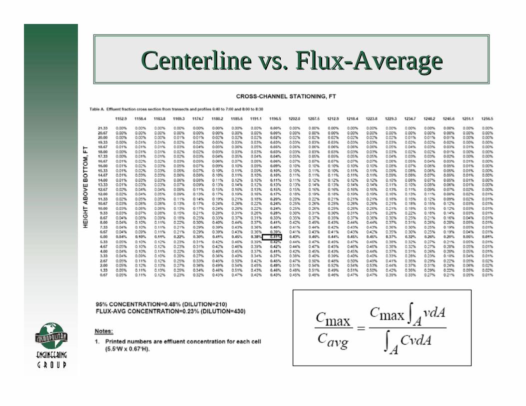
Centerline vs. FluxCenterline vs. Flux--AverageAverage

Quantify Reflux Quantify Reflux –– OverviewOverview

• Method 1: Superposition (Hubbard and Stamper, 1972)

• Method 2: Quasi-steady buildup(EPA, 1992)

• Method 3: Default (rd=0.5)

Quantify Reflux Quantify Reflux –– Method 1Method 1

Quantify Reflux Quantify Reflux –– Method 2Method 2

Reflux Method 2,Alternative 1Reflux Method 2,Alternative 1Mixing Zone Boundary StationMixing Zone Boundary Station

Reflux Method 2, Alternative 2Reflux Method 2, Alternative 2Farfield StationFarfield Station

Reflux Alternative 2 StationingReflux Alternative 2 Stationing

Reflux Reflux –– Method 2, Alternative 2Method 2, Alternative 2

Hydrodynamic Model DevelopmentHydrodynamic Model Development


Station 49 Dye Concentrations

0

2

4

6

8

10

12

Tide

Lev

el (f

t)

0.00

0.20

0.40

0.60

0.80

1.00

1.20

1.40

1.60

Dye C

oncentration (ppb)

Tide (Marysville)Dye ConcentrationModel (ADFAC = 0.00)Corrected2 Period Moving Avg.

26-Aug 27-Aug 28-Aug 29-Aug 30-Aug


Station 56 Dye Concentrations

0

2

4

6

8

10

12

0

0.2

0.4

0.6

0.8

1

1.2

1.4

1.6

Tide (Marysville)Dye ConcentrationModel (ADFAC = 0.00)2 Period Moving Avg.

26-Aug 27-Aug 28-Aug 29-Aug 30-Aug


k = 0.17 day-1

Dye LossDye Loss

• Chlorine quenching• Photochemical decay• Adsorption/settling

Flushing TimeFlushing Time

Monitoring Station

Outfall


Col

umbi

a R

iver

ISCO Station 1ISCO Station 1

Ridgefield WWTP Outfall

Ridgefield WWTP Outfall

City of RidgefieldCity of Ridgefield

ISCO Station 2ISCO Station 2

Lake RiverLake River

Columbia Slough

Columbia Slough

Flushing TimeFlushing TimeStation 1 (downstream)

Station 2 (upstream)


1st High 1st Low 2nd High 2nd Low

Lake River TransectsAugust 30-31, 2004

0.1

1

10

100

-5000 -2500 0 2500 5000 7500 10000

Distance Downstream of Outfall, ft

Dye

Con

cent

ratio

n,pp

b

Residual CirculationResidual Circulation

Dispersion Coefficient Dispersion Coefficient –– TransverseTransverse

Dispersion Coefficient Dispersion Coefficient –– TransverseTransverse

Upstream Mixing Zone Boundary8:50 - 3/4 Flood

0

1

2

3

4

5

6

7

8

9

60 70 80 90 100 110 120 130 140

Distance from Right Bank, ft

Dye

Con

cent

ratio

n, p

pb

1 ft 3 ft 5 ft Model

Centerline Profile8:45 - 3/4 Flood

0

1

2

3

4

5

0 2 4 6 8

Depth, ft

Dye

Con

cent

ratio

n, p

pb

Dispersion Coefficient Dispersion Coefficient –– TransverseTransverseUpstream Mixing Zone Boundary

High Slack

0

1

2

3

4

5

6

7

8

60 70 80 90 100 110 120 130 140


Dye

Con

cent

ratio

n, p

pb

2 ft 2 ft 4 ft 4 ft Model

Dispersion Coefficient Dispersion Coefficient –– TransverseTransverseDownstream Mixing Zone Boundary

13:35 - Mid Ebb

0

1

2

3

4

5

6

7

8

9

10

60 70 80 90 100 110 120 130 140


Dye

Con

cent

ratio

n, p

pb

5 ft 2 ft Model

Centerline Profile13:45 - Mid Ebb

0

2

4

6

8

10

0 2 4 6 8 10

Depth, ft

Dye

Con

cent

ratio

n, p

pb

Stationary Time Series14:00 - Mid Ebb

01234567

14:02:15 14:02:59 14:03:42 14:04:25

Dye

Con

cent

ratio

n, p

pb

3 sec 30 sec 60 sec

Dispersion Coefficient Dispersion Coefficient –– LongitudinalLongitudinal

Transport to Critical AreasTransport to Critical Areas

AlternativeOutfall Sites

Transport to Critical AreasTransport to Critical Areas

Discharge MeasurementDischarge Measurement

ReferencesReferencesTurner Designs Application Notes:

www.turnerdesigns.com/t2/doc/appnotes/tracer_dye.html

General:Kilpatrick, F.A., and E.D. Cobb, Measurement of Discharge Using Tracers, Chapter A16, Techniques of Water-

Resources Investigations of the USGS, Book 3, Application of Hydraulics, USGS, U.S. Department of the Interior,Reston, VA 1985.

Wilson, J.F., E.D. Cobb, and F.,A. Kilpatrick, Fluorometric Procedures for Dye Tracing, Chapter A12. Techniques of Water-Resources Investigations of the USGS, Book 3, Application of Hydraulics, USGS, U.S. Department of theInterior, Reston, VA 1986.

Reflux:

EPA, 1992. Technical Guidance Manual for Performing Waste Load Allocations Book III: Estuaries, Part 3: Use of Mixing Zone Models in Estuarine Waste Load Allocations, U.S. Environmental Protection Agency, EPA/823/R-092/004, section 2.6.

Hubbard, E.F. and W.G. Stamper, 1972. Movement and Dispersion of Soluble Pollutants in the Northeast Cape FearEstuary, North Carolina, Water-supply paper 1873-E, U.S. Geological Survey, United States Department of the Interior.

Chlorine Quenching:

Deaner, D.G. 1973. Effect of Chlorine on Fluorescent Dyes. Journal of Water Pollution Control Federation, V.45:3. 1973. p.507-514.

Turbidity and Adsorption:Ebbesmeyer, C., B. Fox, G. Cannon, M. Kawasi, B. Nairn. 2002. Puget Sound Physical Oceanography Related to the

Triple Junction Region, Brightwater Marine Outfall, Appendix G. Dye Studies. Submitted to King CountyDepartment of Natural Resources and Parks. November 2002.

dye tracer studies in the pacific northwest - pncwa

Documents