dykstra-parson method of caculation.pdf
DESCRIPTION
dykstra-parson method of calculation.this pdf. explain the method of dykstra-parson method calculation.TRANSCRIPT
MODIFICATION OF THE DYKSTRA-PARSONS METHOD TO
INCORPORATE BUCKLEY-LEVERETT DISPLACEMENT THEORY FOR
WATERFLOODS
A Thesis
by
RUSTAM RAUF GASIMOV
Submitted to the Office of Graduate Studies of
Texas A&M University in partial fulfillment of the requirements for the degree of
MASTER OF SCIENCE
August 2005
Major Subject: Petroleum Engineering
ii -
MODIFICATION OF THE DYKSTRA-PARSONS METHOD TO
INCORPORATE BUCKLEY-LEVERETT DISPLACEMENT THEORY FOR
WATERFLOODS
A Thesis
by
RUSTAM RAUF GASIMOV
Submitted to the Office of Graduate Studies of Texas A&M University
in partial fulfillment of the requirements for the degree of
MASTER OF SCIENCE
Approved by: Chair of Committee, Daulat D. Mamora Committee Members, Bryan J. Maggard
Robert R. Berg Head of Department, Stephen A. Holditch
August 2005
Major Subject: Petroleum Engineering
iii -
ABSTRACT
Modification of the Dykstra-Parsons Method to Incorporate Buckley-Leverett
Displacement Theory for Waterfloods. (August 2004)
Rustam Rauf Gasimov, B.S., Azerbaijan State Oil Academy
Chair of Advisory Committee: Dr. Daulat D. Mamora
The Dykstra-Parsons model describes layer 1-D oil displacement by water in
multilayered reservoirs. The main assumptions of the model are: piston-like
displacement of oil by water, no crossflow between the layers, all layers are individually
homogeneous, constant total injection rate, and injector-producer pressure drop for all
layers is the same. Main drawbacks of Dykstra-Parsons method are that it does not take
into account Buckley-Leverett displacement and the possibility of different oil-water
relative permeability for each layer.
A new analytical model for layer 1-D oil displacement by water in multilayered reservoir
has been developed that incorporates Buckley-Leverett displacement and different oil-
water relative permeability and water injection rate for each layer (layer injection rate
varying with time). The new model employs an extensive iterative procedure, thus
requiring a computer program.
To verify the new model, calculations were performed for a two-layered reservoir and
the results compared against that of numerical simulation. Cases were run, in which
layer thickness, permeability, oil-water relative permeability and total water injection
rate were varied.
Main results for the cases studied are as follows. First, cumulative oil production up to
20 years based on the new model and simulation are in good agreement. Second, model
water breakthrough times in the layer with the highest permeability-thickness product
iv -
(kh) are in good agreement with simulation results. However, breakthrough times for the
layer with the lowest kh may differ quite significantly from simulation results. This is
probably due to the assumption in the model that in each layer the pressure gradient is
uniform behind the front, ahead of the front, and throughout the layer after water
breakthrough. Third, the main attractive feature of the new model is the ability to use
different oil-water relative permeability for each layer. However, further research is
recommended to improve calculation of layer water injection rate by a more accurate
method of determining pressure gradients between injector and producer.

v -
DEDICATION
I wish to dedicate my thesis:
To my daughter, Nezrin, the person I love the most, and my wife, Sabina, for her love and support.
To my parents, Rauf and Zulfiya, for all their support, encouragement, sacrifice,
and especially for their unconditional love; I love you both.

vi -
ACKNOWLEDGEMENTS I wish to express my sincere gratitude and appreciation to:
Dr. Daulat D. Mamora, chair of my advisory committee, for his continued help and
support throughout my research. It was great to work with him.
Dr. J. Bryan Maggard, member of my advisory committee, for his enthusiastic and active
participation and guidance during my investigation.
Dr. Robert Berg, member of my advisory committee, for his encouragement to my
research, his motivation to continue studying and his always-good mood.
Finally, I want to express my gratitude and appreciation to all my colleagues in Texas
A&M University: Marylena Garcia, Anar Azimov, and Adedayo Oyerinde.
vii -
TABLE OF CONTENTS
Page
ABSTRACT………... ................................................................................................ iii
DEDICATION……. ................................................................................................... v
ACKNOWLEDGEMENTS ...................................................................................... vi
TABLE OF CONTENTS .......................................................................................... vii
LIST OF FIGURES...................................................................................................... ix
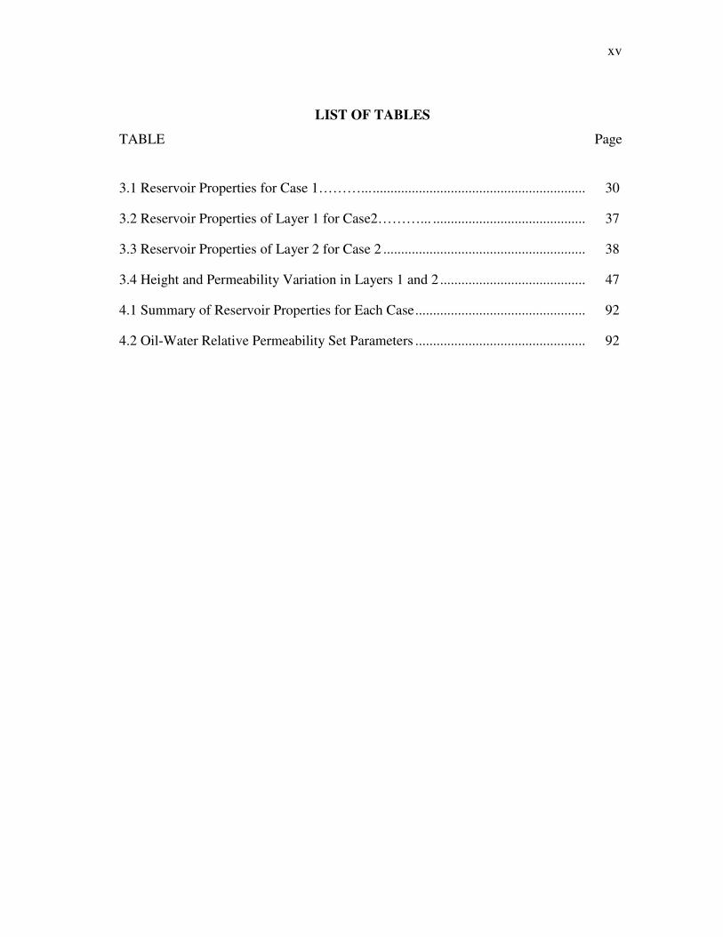
LIST OF TABLES... ................................................................................................. xv
CHAPTER
I INTRODUCTION .......................................................................................... 1
1.1 Buckley-Leverett Model ...................................................................... 1 1.2 Dykstra-Parsons Model........................................................................ 2 1.3 Problem Description ............................................................................ 4 1.4 Objectives ............................................................................................ 5
II LITERATURE REVIEW. ............................................................................... 6
2.1 Buckley-Leverett Frontal Advance Theory ......................................... 6 2.2 Stiles Method .................................................................................... 11 2.3 Dykstra-Parsons Approach ................................................................ 12
III NEW ANALYTICAL METHOD ..................................................................... 18
3.1 Calculation Procedure ......................................................................... 18 3.2 Case 1................................................................................................... 29 3.3 Case 2................................................................................................... 36 3.4 Case 3................................................................................................... 46 3.5 Case 4................................................................................................... 53 3.6 Case 5................................................................................................... 59 3.7 Case 6................................................................................................... 65 3.8 Case 7................................................................................................... 72 3.9 Case 8................................................................................................... 77 3.9 Case 9................................................................................................... 83
viii -
CHAPTER Page
IV SIMULATION MODEL OVERVIEW........................................................... 90
V SUMMARY, CONCLUSIONS AND RECOMMENDATIONS ................... 99
5.1 Summary …......................................................................................... 99 5.2 Conclusions ….. .................................................................................. 99 5.3 Recommendations …......................................................................... 100
NOMENCLATURE................................................................................................. 102
REFERENCES......................................................................................................... 104
APPENDIX A............ .............................................................................................. 106
APPENDIX B...... .................................................................................................... 108
APPENDIX C...... .................................................................................................... 116
VITA..................... ................................................................................................... 172
ix -
LIST OF FIGURES
FIGURE Page
1.1 Oil production: comparison of results based on Dykstra-Parsons model, and numerical simulation for 2-layered model, iw = 800 STB/D.….……................... 4
2.1 Typical fractional flow curve as a function of water saturation ……................... 7 2.2 Water saturation distribution as a function of distance, before breakthrough in
the producing well ................................................................................................ 8 2.3 Water saturation distribution at, and after breakthrough in the producing well... 10 2.4 Schematic piston-like displacement in a layer in the Dykstra-Parsons model…. 14 3.1 Corey type relative permeability curves for Case 1 ………... ............................ 19 3.2 Fractional flow curve for Case 1.... ..................................................................... 21 3.3 Schematic representation of the waterflood process at the moment of
breakthrough in layer 1 ....................................................................................... 24 3.4 Comparison of oil production rate of new analytical model vs. simulation (Case 1)………………………………………………………………………… 31 3.5 Comparison of water injection rate of new analytical model vs. simulation by
layers (Case 1) ……………................................................................................ 32 3.6 Comparison of cumulative oil produced calculated with new analytical model vs. simulation (Case 1) ........................................................................................ 33 3.7 Oil production rates by layers, new analytical model vs. simulation (Case 1) ... 34 3.8 Water production rate by layers, new analytical model vs. simulation (Case 1) 35 3.9 Total water production rate comparison of new analytical model vs. simulation
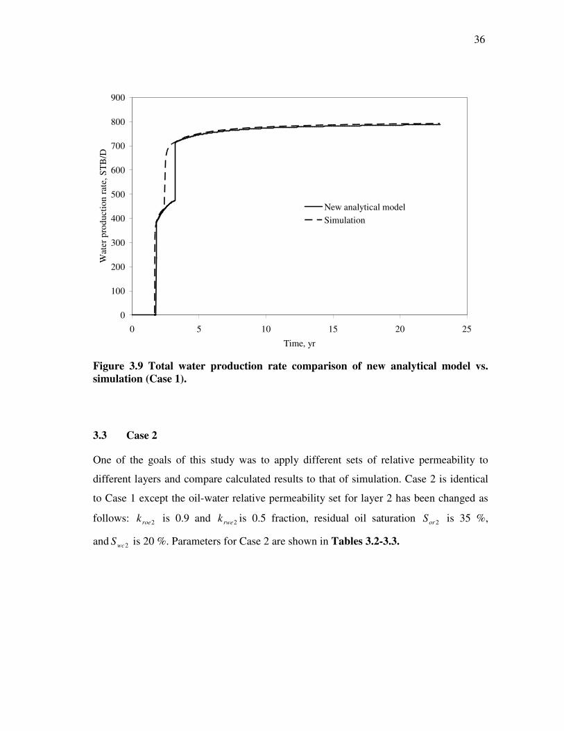
(Case 1).................................................................................................................. 36
x -
FIGURE Page
3.10 Sets of relative permeabilities for layers one and two (Case 2) ....................... 39
3.11 Fractional flow curves for layers one and two respectively (Case 2) ............... 40
3.12 Oil production rate of new analytical model vs. simulation, different sets of relative permeabilities are applied (Case 2) ........................... 41
3.13 Water injection rates by layers of new analytical model vs. simulation, different sets of relative permeabilities are applied(Case 2 )……………....... 42
3.14 Cumulative oil produced comparison of new analytical model vs. simulation, two sets of relative permeability are provided for each layer (Case 2)........... 43
3.15 Oil production rate by layers comparison of new analytical model vs. simulation, two sets of relative permeability are provided for each layer (Case 2)….... .................................................................................................... 44
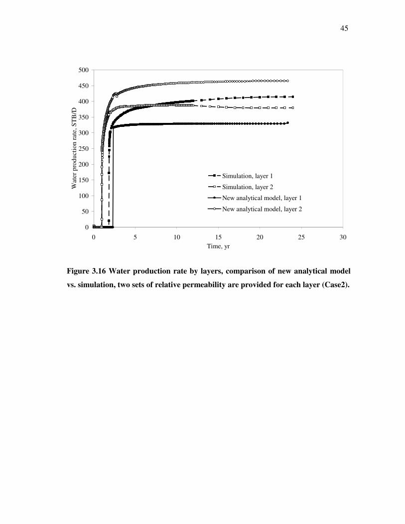
3.16 Water production rate by layers, comparison of new analytical model vs. simulation, two sets of relative permeability are provided for each layer (Case 2)…........................................................................................................ 45
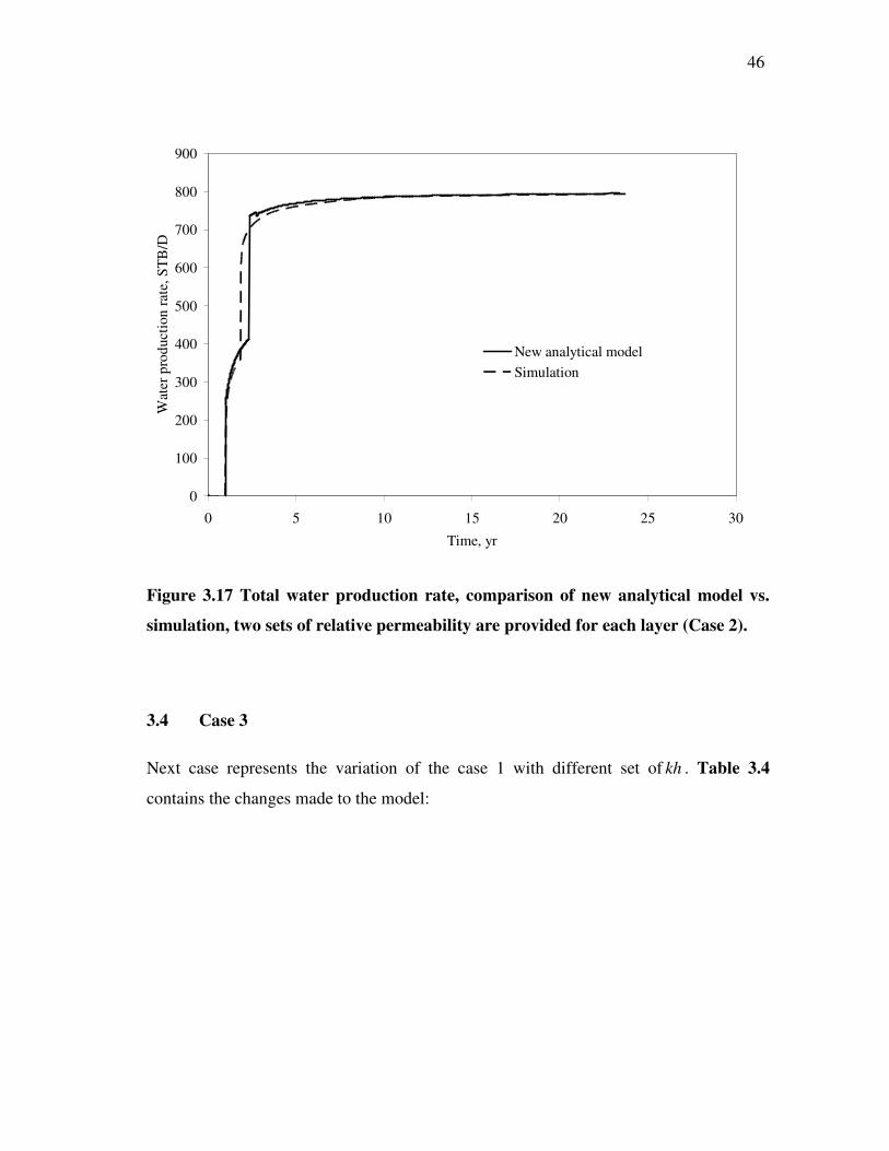
3.17 Total water production rate, comparison of new analytical model vs. simulation, two sets of relative permeability are provided for each layer (Case 2)……………………………………………………………………… 46
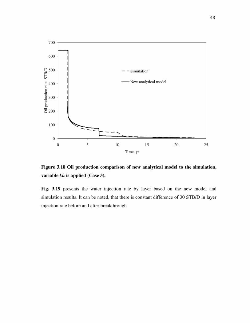
3.18 Oil production comparison of new analytical model to the simulation, variable kh is applied (Case 3) ........................................................................ 48
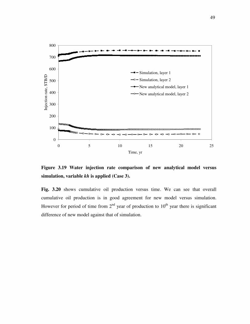
3.19 Water injection rate comparison of new analytical model versus simulation, variable kh is applied (Case 3) ......................................................................... 49
3.20 Cumulative oil produced comparison of new analytical model to the simulation, variable kh is applied (Case 3) ...................................................... 50
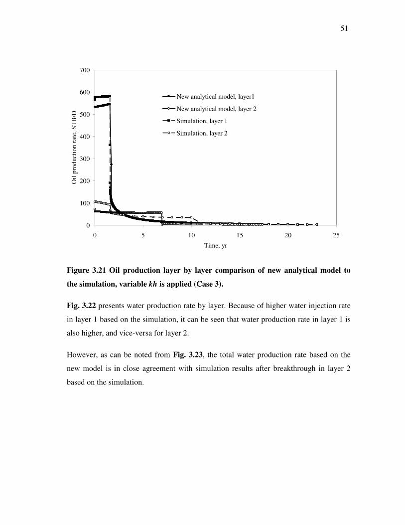
3.21 Oil production layer by layer comparison of new analytical model to the simulation, variable kh is applied (Case 3) ...................................................... 51
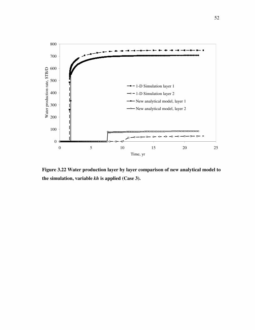
3.22 Water production layer by layer comparison of new analytical model to the simulation, variable kh is applied (Case 3) ............................................... 52
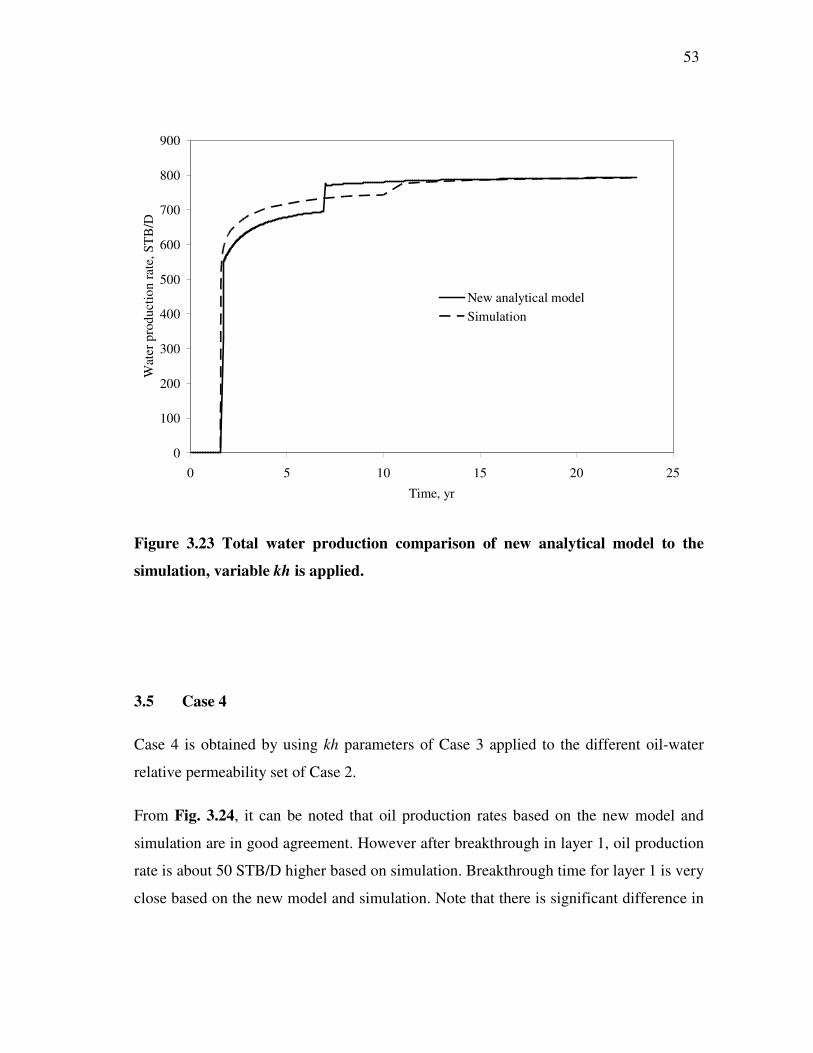
3.23 Total water production comparison of new analytical model to the simulation, variable kh is applied (Case 3) ..................................................... 53
xi -
FIGURE Page
3.24 Total oil production comparison of new analytical model versus simulation, variable kh and relative permeability sets are applied (Case 4) ....................... 54
3.25 Water injection layer by layer comparison of new analytical model to simulation, variable kh and relative permeability sets are applied (Case 4) .... 55
3.26 Cumulative oil produced, comparison of new analytical model to simulation, variable kh and relative permeability sets are applied (Case 4) ....................... 56
3.27 Oil production layer by layer, comparison of new analytical model to simulation, variable kh and relative permeability sets are applied (Case 4) ..... 57
3.28 Water production layer by layer, comparison of new analytical model to simulation, variable kh and relative permeability sets are applied (Case 4) .... 58
3.29 Water production rate, comparison of new analytical model to the simulation, variable kh and relative permeability sets are applied (Case 4) ........................ 59
3.30 Oil production rate, comparison of new analytical model to the simulation, injection rate of 1600 STB/D is applied (Case 5) ............................................. 60
3.31 Water injection rate by layers, comparison of new analytical model to simulation, injection rate of 1600 STB/D is applied (Case 5) .......................... 61
3.32 Cumulative oil production, comparison of new analytical model to simulation, injection rate of 1600 STB/D is applied (Case 5) ............................................. 62
3.33 Oil production rate on layer basis, comparison of new analytical model to simulation, injection rate of 1600 STB/D is applied (Case 5) .......................... 63
3.34 Water production on layer basis, comparison of new analytical model to simulation, injection rate of 1600 STB/D is applied (Case 5) .......................... 64
3.35 Water production rate, comparison of new analytical model to simulation, injection rate of 1600 STB/D is applied (Case 5) ............................................. 65
3.36 Oil production rate, comparison of new analytical model to simulation, 2 relative permeability sets and injection rate of 1600 STB/D are applied (Case 6)……………………………………………………………………….. 66
xii -
FIGURE Page
3.37 Water injection rate by layers, comparison of new analytical model to simulation, 2 relative permeability sets and injection rate of 1600 STB/D are applied (Case 6)……......................................................................................... 67
3.38 Cumulative oil produced, comparison of new analytical model to simulation, 2 relative permeability sets and injection rate of 1600 STB/D are applied (Case 6)………………………………………………………………………... 68
3.39 Oil production rate by layers, comparison of new analytical model to simulation, 2 relative permeability sets and injection rate of 1600 STB/D are applied (Case 6)……......................................................................................... 69
3.40 Water production rate by layers, comparison of new analytical model to simulation, 2 relative permeability sets and injection rate of 1600 STB/D are applied (Case 6)……......................................................................................... 70
3.41 Total water production rate, comparison of new analytical model to simulation, 2 relative permeability sets and injection rate of 1600 STB/D are applied (Case 6)……………………………………………………………………….. 71
3.42 Oil production rate, comparison of new analytical model to simulation, different kh and injection rate of 1600 STB/D are applied (Case 7)................. 72
3.43 Water injection rate by layers, comparison of new analytical model to simulation, different kh and injection rate of 1600 STB/D are applied (Case 7)……………………………………………………………………….. 73
3.44 Cumulative oil produced, comparison of new analytical model to simulation, different kh and injection rate of 1600 STB/D are applied. .............................. 74
3.45 Oil production by layers, comparison of new analytical model to simulation, different kh and injection rate of 1600 STB/D are applied (Case 7)................. 75
3.46 Water production by layers, comparison of new analytical model to simulation, different kh and injection rate of 1600 STB/D are applied (Case 7)................. 76
3.47 Total water production, comparison of new analytical model to simulation, different kh and injection rate of 1600 STB/D are applied (Case 7)................. 77
3.48 Total oil production rate, comparison of new analytical model to simulation, 2 relative permeability sets and injection rate of 1600 STB/D are applied (Case 8)……………………………………………………………………….. 78
xiii -
FIGURE Page
3.49 Water injection rate by layers, comparison of new analytical model to simulation, 2 relative permeability sets and injection rate of 1600 STB/D are applied (Case 8)……......................................................................................... 79
3.50 Cumulative oil, comparison of new analytical model to simulation, 2 relative permeability sets and injection rate of 1600 STB/D are applied (Case 8) ........ 80
3.51 Oil production by layers, comparison of new analytical model to simulation, 2 relative permeability sets and injection rate of 1600 STB/D are applied (Case 8)……………………………………………………………………….. 81
3.52 Water production by layers, comparison of new analytical model to simulation, 2 relative permeability sets and injection rate of 1600 STB/D are applied (Case 8)………………………………………………………………………... 82
3.53 Water production rate, comparison of new analytical model to simulation, 2 relative permeability sets and injection rate of 1600 STB/D are applied (Case 8)…………........................................................................................................ 83
3.54 Oil production rate, comparison of new analytical model to simulation, for 2 identical layers (Case 9) .................................................................................... 84
3.55 Water injection rate by layers, comparison of new analytical model to simulation, for 2 identical layers (Case 9)......................................................... 85
3.56 Cumulative oil produced, comparison of new analytical model to simulation, for 2 identical layers (Case 9) ........................................................................... 86
3.57 Oil production by layers, comparison of new analytical model to simulation, for 2 identical layers (Case 9) ........................................................................... 87
3.58 Water production by layers, comparison of new analytical model to simulation, for 2 identical layers (Case 9) ........................................................................... 88
3.59 Water production rate, comparison of new analytical model to simulation, for 2 identical layers (Case 9) .................................................................................... 89
4.1 Simulation results indicate cumulative oil production with and without grid refinement is practically identical........... ..................................................... 91
4.2 Simulation results for Case 1 at 274 days, showing earlier water breakthrough in layer that has a higher kh .......................................................... 93
xiv -
FIGURE Page
4.3 Simulation results for Case 2 at 274 days, showing faster waterflood displacement in lower layer, which has different oil-water relative permeability……................................................................................................. 94
4.4 Simulation results for Case 3 at 274 days, showing faster water front propagation in upper layer that has a higher kh value......................................... 94
4.5 Simulation results for Case 4 at 274 days, showing faster oil displacement in upper layer that has a higher kh value....................................... 95
4.6 Simulation results for Case 5 at 274 days, showing that flood front advanced more than that in Case 1, as water injection rate was doubled............................ 95
4.7 Simulation results for Case 6 at 274 days, showing similarity to Case 2 except that lower layer broke through................................................................. 96
4.8 Simulation results for Case 7 at 274 days, showing faster front propagation than that in Case 3 due to increased injection rate .............................................. 96
4.9 Simulation results for Case 8 at 274 days, showing faster front propagation than that in Case 4 due to increased injection rate .............................................. 97
4.10 Simulation results for Case 9 at 274 days, showing identical displacement in both layers, as both layers have identical reservoir properties………................................................................................................. 97
4.11 Injector-producer pressure drop for simulation model on example of Case 3……….. .................................................................................................... 98
xv -
LIST OF TABLES
TABLE Page
3.1 Reservoir Properties for Case 1………............................................................... 30
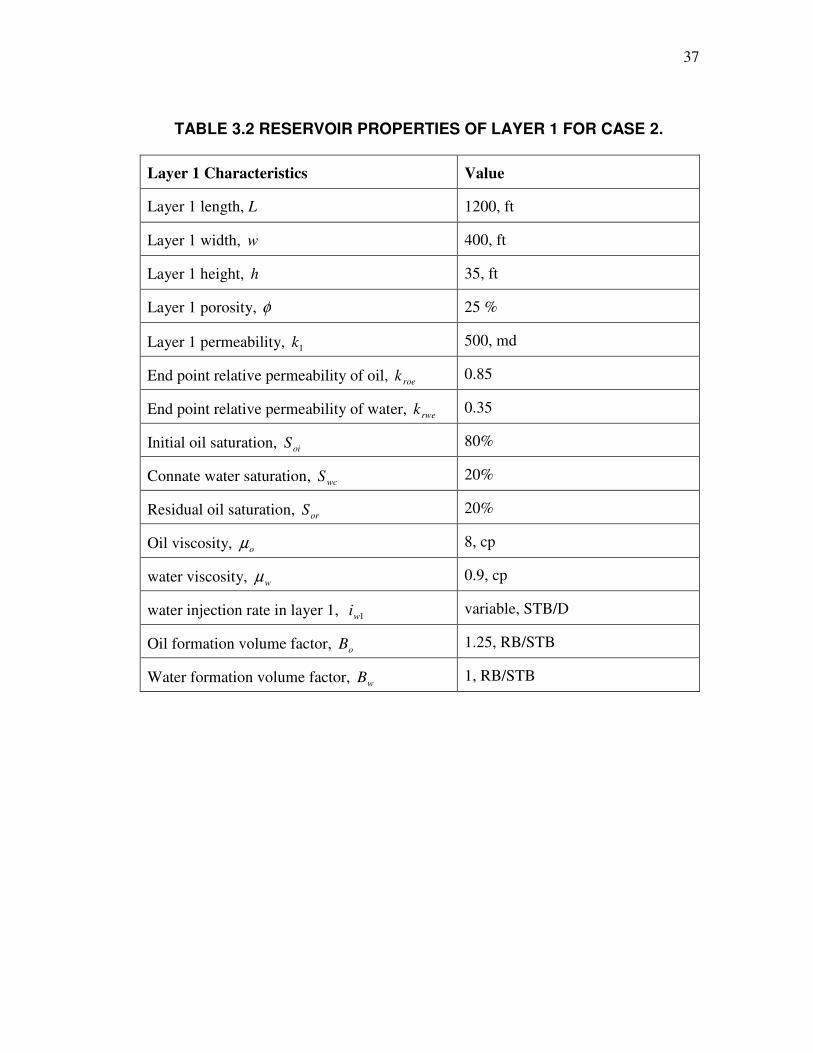
3.2 Reservoir Properties of Layer 1 for Case2………... ........................................... 37
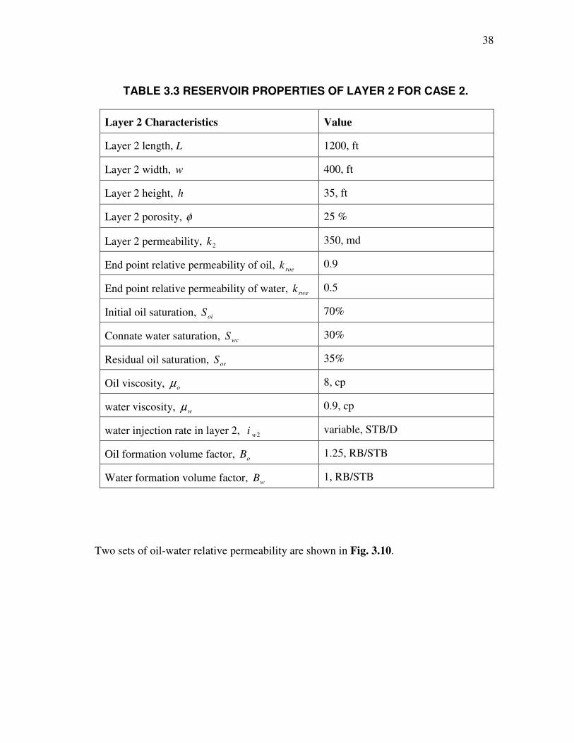
3.3 Reservoir Properties of Layer 2 for Case 2 ......................................................... 38
3.4 Height and Permeability Variation in Layers 1 and 2 ......................................... 47
4.1 Summary of Reservoir Properties for Each Case................................................ 92
4.2 Oil-Water Relative Permeability Set Parameters ................................................ 92
1 -
CHAPTER I
2. INTRODUCTION
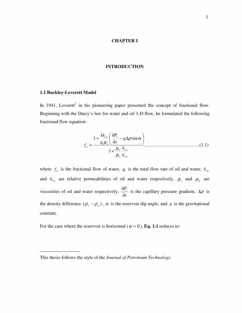
1.1 Buckley-Leverett Model
In 1941, Leverett1 in his pioneering paper presented the concept of fractional flow.
Beginning with the Darcy’s law for water and oil 1-D flow, he formulated the following
fractional flow equation:
rw
ro
o
w
c
ot
ro
w
kk
gxP
qkk
f
µµ
αρµ
+
��
���
� ∆−∂∂+
=1
sin1,...…………………….…….(1.1)
where wf is the fractional flow of water, tq is the total flow rate of oil and water, rok
and rwk are relative permeabilities of oil and water respectively, oµ and wµ are
viscosities of oil and water respectively, xPc
∂∂
is the capillary pressure gradient, ρ∆ is
the density difference )( wo ρρ − , α is the reservoir dip angle, and g is the gravitational
constant.
For the case where the reservoir is horizontal ( 0=α ), Eq. 1.1 reduces to:
_________________
This thesis follows the style of the Journal of Petroleum Technology.
2 -
rw
ro
o
ww
kk
f
µµ
+=
1
1. …………………………………………...(1.2)
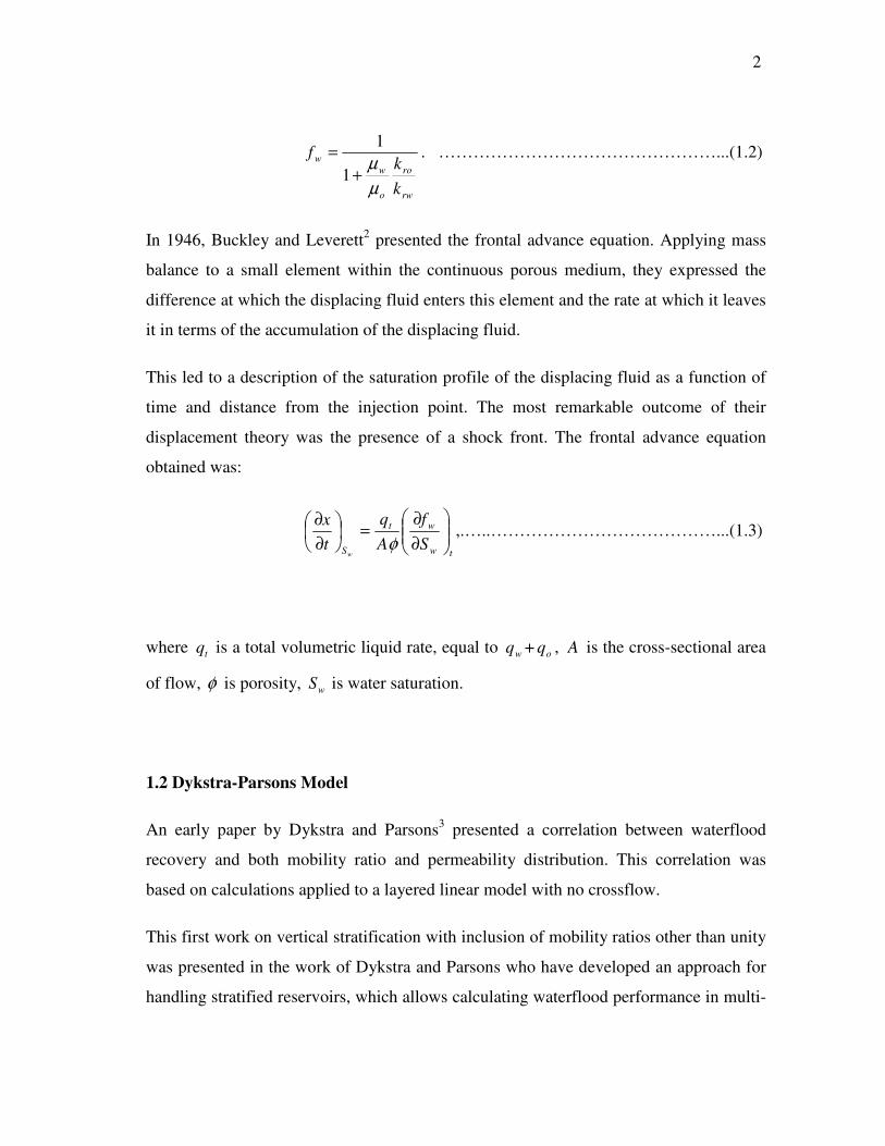
In 1946, Buckley and Leverett2 presented the frontal advance equation. Applying mass
balance to a small element within the continuous porous medium, they expressed the
difference at which the displacing fluid enters this element and the rate at which it leaves
it in terms of the accumulation of the displacing fluid.
This led to a description of the saturation profile of the displacing fluid as a function of
time and distance from the injection point. The most remarkable outcome of their
displacement theory was the presence of a shock front. The frontal advance equation
obtained was:
tw
wt
S Sf
Aq
tx
w
���
����
�
∂∂
=��
���
�
∂∂
φ,.…..…………………………………...(1.3)
where tq is a total volumetric liquid rate, equal to wq + oq , A is the cross-sectional area
of flow, φ is porosity, wS is water saturation.
1.2 Dykstra-Parsons Model
An early paper by Dykstra and Parsons3 presented a correlation between waterflood
recovery and both mobility ratio and permeability distribution. This correlation was
based on calculations applied to a layered linear model with no crossflow.
This first work on vertical stratification with inclusion of mobility ratios other than unity
was presented in the work of Dykstra and Parsons who have developed an approach for
handling stratified reservoirs, which allows calculating waterflood performance in multi-
3 -
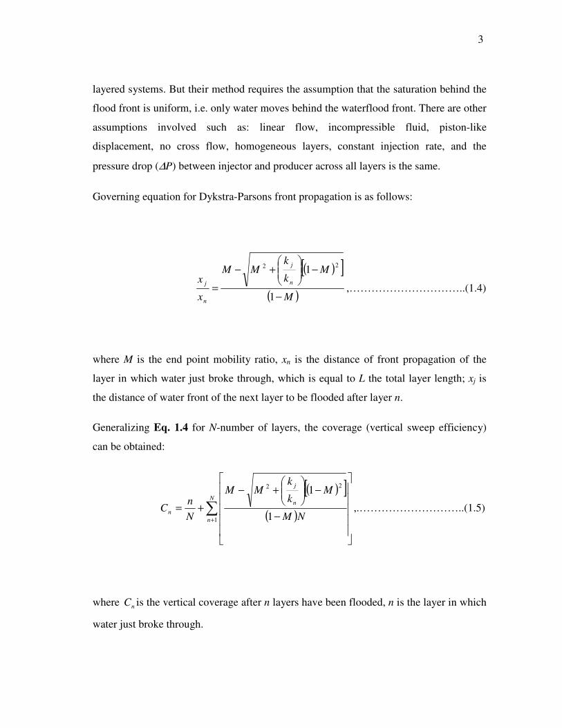
layered systems. But their method requires the assumption that the saturation behind the
flood front is uniform, i.e. only water moves behind the waterflood front. There are other
assumptions involved such as: linear flow, incompressible fluid, piston-like
displacement, no cross flow, homogeneous layers, constant injection rate, and the
pressure drop (∆P) between injector and producer across all layers is the same.
Governing equation for Dykstra-Parsons front propagation is as follows:
( )[ ]( )M
Mk
kMM
x
x n
j
n
j
−
−���
����
�+−
=1
1 22
,…………………………..(1.4)
where M is the end point mobility ratio, xn is the distance of front propagation of the
layer in which water just broke through, which is equal to L the total layer length; xj is
the distance of water front of the next layer to be flooded after layer n.
Generalizing Eq. 1.4 for N-number of layers, the coverage (vertical sweep efficiency)
can be obtained:
( )[ ]( )�
+
�����
�����
�
−
−���
����
�+−
+=N
n
n
j
n NM
Mk
kMM
Nn
C1
22
1
1
,.………………………..(1.5)
where nC is the vertical coverage after n layers have been flooded, n is the layer in which
water just broke through.
4 -
1.3 Problem Description
For many years analytical models have been used to estimate performance of waterflood
projects. The Buckley-Leverett frontal advance theory and Dykstra-Parsons method for
stratified reservoirs have been used for this purpose, but not in combination for stratified
reservoirs with different kh and oil-water relative permeability.
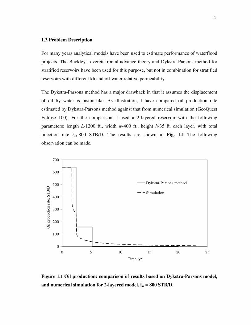
The Dykstra-Parsons method has a major drawback in that it assumes the displacement
of oil by water is piston-like. As illustration, I have compared oil production rate
estimated by Dykstra-Parsons method against that from numerical simulation (GeoQuest
Eclipse 100). For the comparison, I used a 2-layered reservoir with the following
parameters: length L-1200 ft., width w-400 ft., height h-35 ft. each layer, with total
injection rate iwt-800 STB/D. The results are shown in Fig. 1.1 The following
observation can be made.
0
100
200
300
400
500
600
700
0 5 10 15 20 25
Time, yr
Oil
prod
uctio
n ra
te, S
TB/D
Dykstra-Parsons method
Simulation
Figure 1.1 Oil production: comparison of results based on Dykstra-Parsons model,
and numerical simulation for 2-layered model, iw = 800 STB/D.
5 -
First, the water breakthrough time based on simulation is significantly earlier compared
to that from Dykstra-Parsons method. Second, cumulative oil produced at the moment of
breakthrough in layer 1, is more for the Dykstra-Parsons analytical model compared to
simulation. This is because Dykstra-Parsons model assumes that at breakthrough, all
moveable oil has been swept from layer 1, whereas in the simulation model at
breakthrough, there is still moveable oil behind the front.
1.4 Objectives
The goal of this research is to modify the Dykstra-Parsons method for 1-D oil
displacement by water in such a manner that it would be possible to incorporate the
Buckley-Leverett frontal advance theory. This would require modeling fractional flow
behind the waterflood front instead of assuming piston-like displacement. By
incorporating Buckley-Leverett displacement, a more accurate analytical model of oil
displacement by water is expected. Permeability-thickness and oil-water relative
permeability will be different for each layer, with no crossflow between the layers. The
analytical model results (injection rate, water and oil production rate) will be compared
against simulation results to ensure the validity of the analytical model.
6 -
CHAPTER II
2. LITERATURE REVIEW
2.1 Buckley-Leverett Frontal Advance Theory
Since the original paper of Dykstra-Parsons, a great number of papers have suggested
some modifications to the basic approach. The literature review gives the reader an
overview of these modifications.
Buckley and Leverett (1946): The Buckley-Leverett frontal advance theory considers the
mechanism of oil displacement by water in a linear 1-D system. An equation was
developed for calculating the frontal advance rate. In the Buckley-Leverett approach oil
displacement occurred under so-called diffuse flow condition, which means that fluid
saturations at any point in the linear displacement path are uniformly distributed with
respect to thickness.
The fractional flow of water, at any point in the reservoir, is defined as
wo
ww qq
qf
+= ,...……………………………………………....(2.1)
where wq is water flow rate, and oq is oil flow rate.
Using Darcy’s law for linear one dimensional flow of oil and water, considering the
displacement in a horizontal reservoir, and neglecting the capillary pressure gradient we
get the following expression:
7 -
o
ro
rw
ww k
k
f
µµ
+=
1
1. …………..……………………………….(2.2)
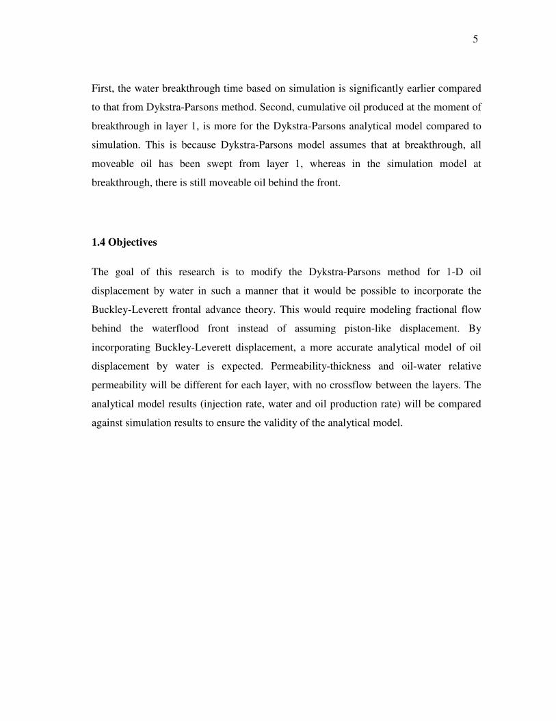
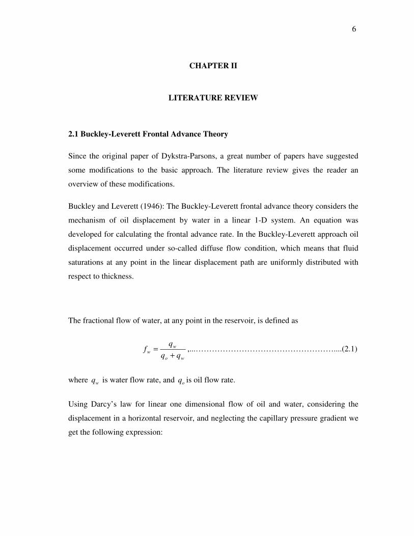
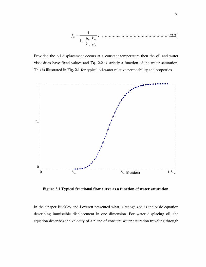
Provided the oil displacement occurs at a constant temperature then the oil and water
viscosities have fixed values and Eq. 2.2 is strictly a function of the water saturation.
This is illustrated in Fig. 2.1 for typical oil-water relative permeability and properties.
Figure 2.1 Typical fractional flow curve as a function of water saturation.
In their paper Buckley and Leverett presented what is recognized as the basic equation
describing immiscible displacement in one dimension. For water displacing oil, the
equation describes the velocity of a plane of constant water saturation traveling through
1-S orwc Sw S
fw
1
0 0 (fraction)
8 -
the linear system. Assuming the diffuse flow conditions and conservation of mass of
water flowing through volume element Adx :
ww S
w
wiS dS
dfAW
xφ
= ,...………………………………………….(2.3)
where iW is the cumulative water injected and it is assumed, as an initial condition, that
iW = 0 when t = 0.
There is a mathematical difficulty encountered in applying this technique, which exists
due to the nature of the fractional flow curve creating a saturation discontinuity or a
shock front.
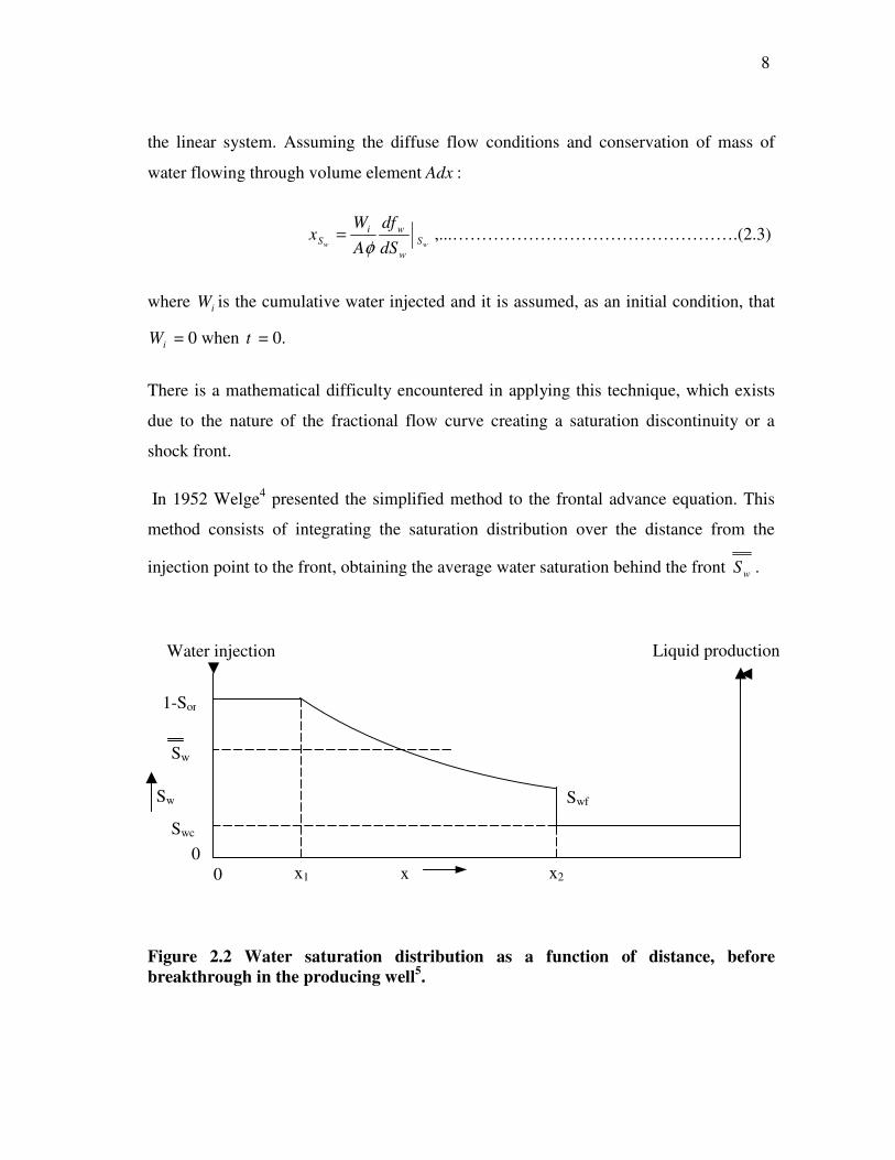
In 1952 Welge4 presented the simplified method to the frontal advance equation. This
method consists of integrating the saturation distribution over the distance from the
injection point to the front, obtaining the average water saturation behind the front wS .
Figure 2.2 Water saturation distribution as a function of distance, before breakthrough in the producing well5.
1-Sor
x1 x2x
Swc
Swf
Sw
Water injection Liquid production
00
Sw
9 -
Fig. 2.2 presents water saturation profile as a function of distance.
Applying the simple material balance:
)(2 wcwi SSAxW −= φ ,...……………………………………...(2.4)
where wS is average water saturation behind the front, 1x is distance in the reservoir
totally flooded by water, 2x is distance of waterflood front location.
Eqs. 2.3 and 2.4 yield the following solution to wS :
wfw
w
iwcw
SdSdfAx
WSS
1
2
==−φ
. …..………………………….(2.5)
The expression for the average water saturation behind the front can also be obtained by
direct integration of the saturation profile as
2
1
2
1
)1(
x
dxSxS
S
x
xwor
w
�+−
= . …………………………………(2.6)
And since wSx α
wSwdS
df the Eq. 2.6 can be expressed as
wf
or
Sw
w
x
x w
wwS
w
wor
w
dSdf
dSdf
dSdSdf
S
S� ��
�
����
�+−
=−
2
1
1)1(
. ……………………(2.7)
After rearranging Eq. 2.7,
10 -
( )wfwf S
w
wSwwfw dS
dffSS −+= 1 . …………………………...(2.8)
Note that for 0=wf , Eq. 2.8 reduces to Eq. 2.5.
Cumulative oil production at the breakthrough can be expressed by following equation:
( )wbt
w
wwcwbtiDiDbtpDbt
SdSdf
SStqWN1=−=== ,..................……………………...(2.9)
where pDbtN is dimensionless cumulative oil produced at the moment of breakthrough,
iDbtW is dimensionless cumulative water injected at the moment of breakthrough.
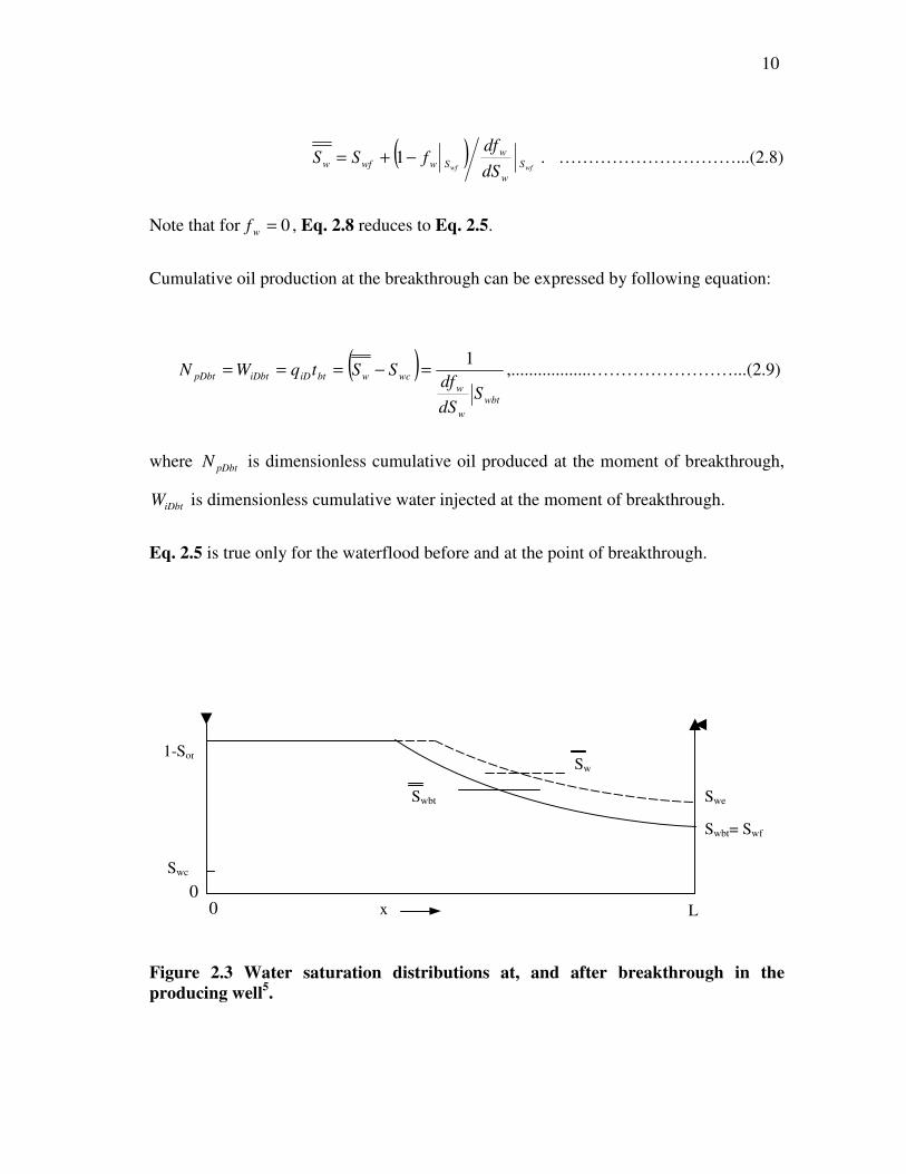
Eq. 2.5 is true only for the waterflood before and at the point of breakthrough.
Figure 2.3 Water saturation distributions at, and after breakthrough in the producing well5.
1-Sor
L x
Swc
Swbt= Swf
Swe Swbt
Sw
00
11 -
From the Fig. 2.3, Swe is the current value of the water saturation at the producing well
after water breakthrough. Water saturation by the Welge technique gives:
( )weS
w
wwewew
dSdf
fSS1
1−+= . ……………………………..(2.10)
Following Eq. 2.9 oil recovery after water breakthrough can be expressed as:
( ) ( ) iDwewcwewcwpD WfSSSSN −+−=−= 1 . ……………...(2.11)
2.2 Stiles Method
Stiles6 (1949): This method for predicting the performance of waterflood operations
basically involves accounting for permeability variations, vertical distribution of flow
capacity kh. Most important assumption was that within the reservoir of various
permeabilities injected water sweeps first the zones of higher permeability and that first
breakthrough occurs in these layers. The different flood-front positions in liquid-filled,
linear layers having different permeabilities, each layer insulated from the others. Stiles
assumes that the rate of water injected into each layer depends only upon the kh of that
layer. This is equivalent to assuming a mobility ratio of unity. Also it is assumed that
fluid flow is linear and the distance of penetration of the flood front is proportional to
permeability-thickness product.
The Stiles method assumes that there is piston-like displacement of oil, so that after
water breakthrough in a layer, only water is produced from that layer. After water
breakthrough, the producing WOR is found as follows:
oro
o
w
rw Bk
kWOR
µµκ
κ−
=1
,…...………………………………..(2.12)
12 -
where κ is the fraction of the total flow capacity represented by layers having water
breakthrough. In addition, the Stiles method assumes a unit mobility ratio. In his work
Stiles rearranged the layers depending on their permeability in descending manner.
Later Johnson7 developed a graphical approach that simplified the consideration of layer
permeability and porosity variations. Layer properties were chosen such that each had
equal flow capacities so that the volumetric injection rate into each layer was the same.
2.3 Dykstra-Parsons Approach
Dykstra and Parsons (1950): An early paper presented a correlation between waterflood
recovery and both mobility ratio and permeability distribution. This correlation was
based on calculations applied to a layered linear model with no crossflow.
More than 200 flood pot tests were made on more than 40 California core samples in
which initial fluid saturations, mobility ratios, producing WOR’s, and fractional oil
recoveries were measured. The permeability distribution was measured by the
coefficient of permeability variation.
The correlations presented by Dykstra-Parsons related oil recovery at producing WOR’s
of 1, 5, 25, and 100 as a fraction of the oil initially in place to the permeability variation,
mobility ratio, and the connate-water and flood-water saturations. The values obtained
assume a linear flood since they are based upon linear flow tests.
The Dykstra-Parsons method considers the effect of vertical variations of horizontal
permeabilities for the waterflood performance calculation. Similar to the Stiles method,
permeabilities are arranged in descending order. Following is a full list of assumptions
for Dykstra-Parsons approach.
(1) Linear flow
13 -
(2) Incompressible displacement
(3) Piston-like displacement
(4) Each layer is a homogenous layer
(5) No crossflow between layers
(6) Pressure drop for all layers is the same
(7) Constant water injection rate
(8) Velocity of the front is proportional to absolute permeability and end point
mobility ratio of the layer
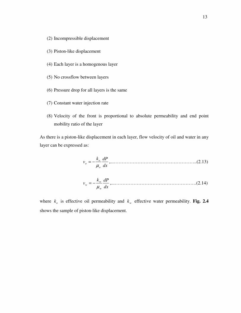
As there is a piston-like displacement in each layer, flow velocity of oil and water in any
layer can be expressed as:
dxdPk
vo
oo µ
−= ,...……………………………………………..(2.13)
dxdPk
vw
ww µ
−= ,...…………………………………………….(2.14)
where ok is effective oil permeability and wk effective water permeability. Fig. 2.4
shows the sample of piston-like displacement.
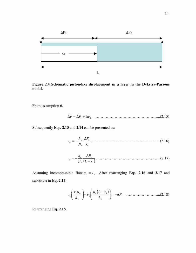
14 -
Figure 2.4 Schematic piston-like displacement in a layer in the Dykstra-Parsons model.
From assumption 6,
21 PPP ∆+∆=∆ . …………………………………………...(2.15)
Subsequently Eqs. 2.13 and 2.14 can be presented as:
1
1
xPk
vw
ww
∆−=
µ ,...…………………………………………...(2.16)
( )1
2
xLPk
vo
oo −
∆−=
µ. ………………………………………...(2.17)
Assuming incompressible flow, wo vv = . After rearranging Eqs. 2.16 and 2.17 and
substitute in Eq. 2.15:
( )
Pk
xLv
kx
vo
oo
w
ww ∆−=��
�
����
� −+���
����
� 11 µµ. ……………………...(2.18)
Rearranging Eq. 2.18,
L
∆P1 ∆P2
x1
15 -
( )11 xL
kx
k
Pv
o
o
w
wo
−+
∆−= µµ . …………………………………(2.19)
Effective permeability for oil and water can be expressed as roo kkk = , rww kkk = , which
on substituting into Eq. 2.19 yields:
( )11
1
xLk
xk
Pkv
ro
o
rw
wo
−+
∆−= µµ . …………………………………(2.20)
Using assumption that rwk and rok are the same for all layers:
( )
( )���
����
�−+
���
����
�−+
=
iro
oi
rw
w
ro
o
rw
w
i
o
oi
xLk
xk
xLk
xk
kk
vv
µµ
µµ11
1
. …………………………..(2.21)
The end point mobility ratio is defined as:
roe
o
w
rweep k
kM
µµ
= . …………………………………………...(2.22)
Eq. 2.21 may be rearranged and integrated with respect to x to give the following
expression:
( ) ( ) 01211
2
=+−��
���
�+��
���
�− epii
epi
ep Mkk
Lx
MLx
M . …………...(2.23)
Eq. 2.23 is a quadratic equation, therefore solving forLxi :
16 -
( )( )1
15.0
2
1
2
−
���
����
�−+±
=ep
epi
epepi
M
Mkk
MM
Lx
. …….………………(2.24)
Generalizing Dykstra-Parsons Eq. 2.24 for any two layers with jn kk > , and n is the
layer, in which water just broke through:
( )( )1
15.0
22
−
���
����
�−+−
=ep
epn
jepep
n
j
M
Mk
kMM
x
x. ……………………(2.25)
Finally expression for the coverage can be obtained:
( )( )�
�
+
+
�����
�����
�
−
���
����
�−+−
+=+
=N
n ep
epn
jepep
N
n n
j
n MN
Mk
kMM
nN
x
xn
C1
5.022
1
1
1
. …......(2.26)
And after rearrangement:
( ) ( )N
Mk
kMM
MM
MnNn
C
N
nep
n
jepep
epep
ep
n
�+
���
����
�−+−
−−
−−
+= 1
5.022 1
11
1,…….....(2.27)
where N is the total number of layers.
Kufus and Lynch8 (1959): Kufus and Lynch in their paper presented work which can
incorporate Buckley-Leverett theory in the Dykstra-Parsons calculations. Important
assumptions Kufus and Lynch have made were that all layers have same relative
permeability curves to oil and water and water injection rate in each layer is constant
value and dependent only on the absolute permeability and on fraction of average water
relative permeability to average fractional flow in the current layer, which is made
17 -
similar to Dykstra-Parsons model.. The data presented in the paper were valid only for
viscosity ratio of unity. And as in Dykstra-Parsons it was assumed that relative
permeabilities to oil and water were same for all layers.
Mobility ratio was represented by following equation:
avw
rw
row
o
fk
kM ��
�
����
�=
'µµ
,...………………………………………(2.28)
where rok' is the oil relative permeability ahead of the waterflood front. Using
computation procedure the major parameters can be calculated.
Hiatt9 (1958): Hiatt presented a detailed prediction method concerned with the vertical
coverage or vertical sweep efficiency attained by a waterflood in a stratified reservoir.
Using a Buckley-Leverett type of displacement, he considered, for the first time,
crossflow between layers. The method is applicable to any mobility ratio, but is difficult
to apply.12
Warren and Cosgrove10 (1964): presented an extension of Hiatt’s original work. They
considered both mobility ratio and crossflow effects in a reservoir whose permeabilities
were log-normally distributed. No initial gas saturation was allowed, and piston-like
displacement of oil by water was assumed. The displacement process in each layer is
represented by a sharp “pseudointerface” as in the Dykstra-Parsons model.
Reznik11 et al. (1984): In this work the original Dykstra-Parsons discrete solution has
been extended to continuous, real time basis. Work has been made considering two
injection constraints: pressure and rate. This analytical model assumes piston-like
displacement. The purpose of the paper was to extend the analytical, but discrete,
stratification model of Dykstra-Parsons to analytically continuous space-time solutions.
The Reznik et al. work retained the piston-like displacement assumption.
18 -
CHAPTER III
3. NEW ANALYTICAL METHOD
The main drawbacks of the Dykstra-Parsons method are that (1) oil displacement by
water is piston-like, and (2) relative permeability end-point values are the same for all
layers. Applying Buckley-Leverett theory to each layer is also not correct because it
would mean that water injection rate is (1) constant for each layer, and (2) proportional
to the kh of each layer.
Thus a new analytical model has been developed with the following simplifying main
assumptions:
(1) Pressure drop for all layers is the same.
(2) Total water injection rate is constant.
(3) Oil-water relative permeabilities may vary for each layer.
(4) Water injection rate in each layer may vary.
3.1 Calculation procedure
The equations and steps used in the new analytical method are as follows. For simplicity,
the method has been applied to a 2-layered system with no cross-flow.
Step 1-Calculate oil-water relative permeabilities
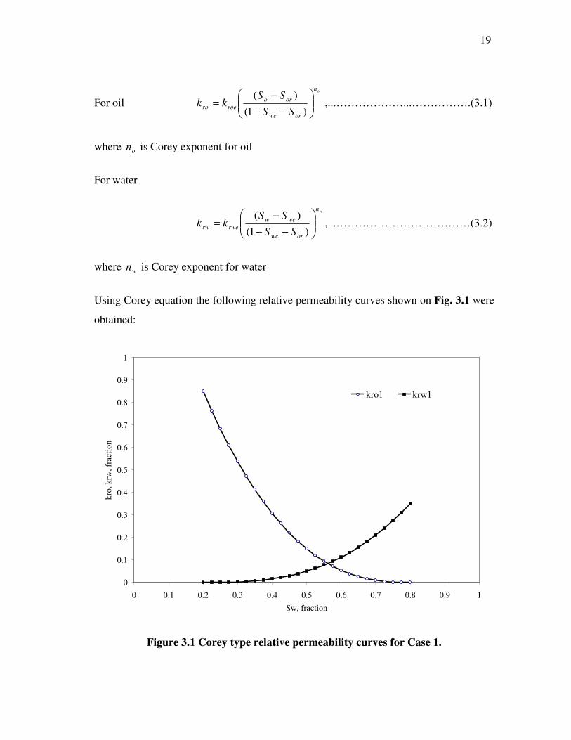
For relative permeability calculation Corey13 type relative permeability curves for oil
and water have been used.
19 -
For oil on
orwc
ororoero SS
SSkk ��
�
����
�
−−−
=)1(
)( ,...………………...…………….(3.1)
where on is Corey exponent for oil
For water
wn
orwc
wcwrwerw SS
SSkk ��
�
����
�
−−−
=)1(
)(,...………………………………(3.2)
where wn is Corey exponent for water
Using Corey equation the following relative permeability curves shown on Fig. 3.1 were
obtained:
0
0.1
0.2
0.3
0.4
0.5
0.6
0.7
0.8
0.9
1
0 0.1 0.2 0.3 0.4 0.5 0.6 0.7 0.8 0.9 1
Sw, fraction
kro,
krw
, fra
ctio
n
kro1 krw1
Figure 3.1 Corey type relative permeability curves for Case 1.
20 -
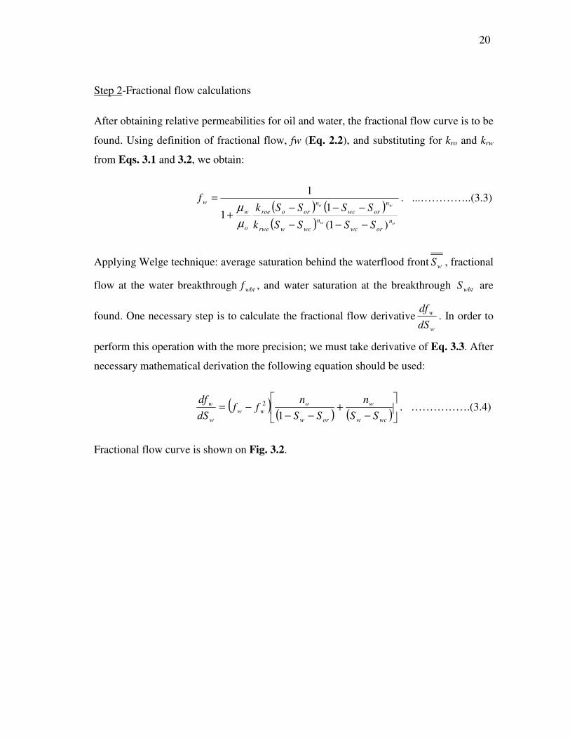
Step 2-Fractional flow calculations
After obtaining relative permeabilities for oil and water, the fractional flow curve is to be
found. Using definition of fractional flow, fw (Eq. 2.2), and substituting for kro and krw
from Eqs. 3.1 and 3.2, we obtain:
( ) ( )( ) ow
wo
norwc
nwcwrwe
norwc
nororoe
o
ww
SSSSk
SSSSkf
)1(
11
1
−−−−−−
+=
µµ
. ...…………..(3.3)
Applying Welge technique: average saturation behind the waterflood front wS , fractional
flow at the water breakthrough wbtf , and water saturation at the breakthrough wbtS are
found. One necessary step is to calculate the fractional flow derivativew
w
dSdf
. In order to
perform this operation with the more precision; we must take derivative of Eq. 3.3. After
necessary mathematical derivation the following equation should be used:
( ) ( ) ( )�
��
−+
−−−=
wcw
w
orw
oww
w
w
SSn
SSn
ffdSdf
12 . …………….(3.4)
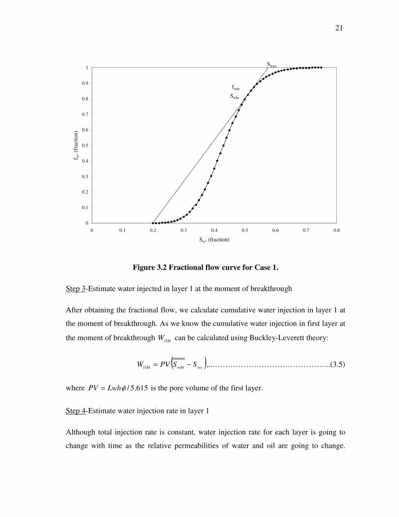
Fractional flow curve is shown on Fig. 3.2.
21 -
0
0.1
0.2
0.3
0.4
0.5
0.6
0.7
0.8
0.9
1
0 0.1 0.2 0.3 0.4 0.5 0.6 0.7 0.8
Sw, (fraction)
f w, (
frac
tion)
Swbt
fwbt
Swav
Figure 3.2 Fractional flow curve for Case 1.
Step 3-Estimate water injected in layer 1 at the moment of breakthrough
After obtaining the fractional flow, we calculate cumulative water injection in layer 1 at
the moment of breakthrough. As we know the cumulative water injection in first layer at
the moment of breakthrough btiW 1 can be calculated using Buckley-Leverett theory:
( )wcwbtbti SSPVW −=1 ,...……………………………………...(3.5)
where 615.5/φLwhPV = is the pore volume of the first layer.
Step 4-Estimate water injection rate in layer 1
Although total injection rate is constant, water injection rate for each layer is going to
change with time as the relative permeabilities of water and oil are going to change.
22 -
Because of that we can not use the following approach in calculating the water injection
rate for layer 1:
wtw ikhhk
i�
= 11 . …….………………………………………...(3.6)
But Eq. 3.6 can be used as an initial estimate or guess in the iterative procedure.
Step 5-Calculation of the time of breakthrough
After obtaining value of water injection rate in layer 1 using Eq. 3.6, the following steps
should be taken: Using Eq. 3.5 estimate water injection rate in layer 1, after which
calculate time of breakthrough
1
1
w
btibt i
Wt = . ..…………………………………………………(3.7)
Step 6-Calculation of total cumulative water injected
In this step total cumulative water injected at the time of breakthrough is calculated,
btwtitbt tiW = . ..……………………………………………….(3.8)
Step 7-Calculation of water injected in layer 2
Since the total cumulative water injection and cumulative water injection in layer 1 are
available, from material balance the cumulative water injection in layer 2 can be
obtained.
btiitbti WWW 12 −= . …..………………………………………(3.9)
Step 8-Calculation of average water saturation in layer 2, pore volume displaced by
water in layer 2 and location of waterflood in layer 2
23 -
Described process occurs at Buckley-Leverett frontal displacement, so the average
water saturation of second layer behind the front before breakthrough is constant and
equal to first layer average water saturation behind the front at the moment of
breakthrough.
22
22
2 '1
wcw
wcx
iw S
fS
PVW
S +=+= ,...…………………………(3.10)
where 2'wf is constant and equal to btwf 1' , xPV is pore volume of layer 2 displaced by
water. From Eq. 3.10 we can obtain xPV :
22 'wix fWPV = . ……………………………………………(3.11)
Main point of this calculation is to find x – the location of waterflood front in layer 2. It
can be done using following expression
615.5/φxwhPVx = . ………………………………………(3.12)
The importance of x – value is crucial for the calculations after the layer 1 broke
through as it is only controlling parameter specifying at which step after layer 1 broke
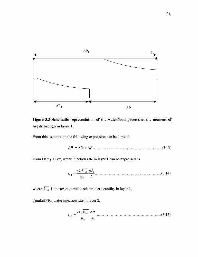
through layer 2 is going to break through. Fig. 3.3 shows waterflood process at the
moment of water breakthrough in layer 1.
Step 9-Recalculation of water injection rate in layer 1
We need to develop different approach for calculating 1wi ; as it has been assumed the
pressure gradient across all layers is the same
24 -
Figure 3.3 Schematic representation of the waterflood process at the moment of
breakthrough in layer 1.
From this assumption the following expression can be derived:
'21 PPP ∆+∆=∆ . …..………………………………………(3.13)
From Darcy’s law, water injection rate in layer 1 can be expressed as
LPkck
iw
rww
1111
∆=µ
,.…………………………………………..(3.14)
where 1rwk is the average water relative permeability in layer 1.
Similarly for water injection rate in layer 2,
2
2222 x
Pkcki
w
rww
∆=µ
,.………………………………………....(3.15)
L ∆P1
∆P2 ∆P’
25 -
where xP2∆
is pressure gradient of the region in layer 2, which has been displaced by
water.
Using Darcy’s law again for oil flow in layer 2
( )2
222
'xL
Pkckq
o
roo −
∆=µ
. …..…………………..……………(3.16)
For incompressible flow ooww BqBi 22 = ; applying Eq. 3.13 to Eqs. 3.14-3.16 we obtain
the following expression:
22
22
22
22
11
1 )(
ro
ow
rw
ww
rw
ww
kkxLi
kk
xi
kk
Li µµµ −+= . ……………………...(3.17)
Knowing that total water injection rate is constant, simple material balance expression
follows:
12 wwtw iii −= . ……………………………………………..(3.18)
Substituting Eq. 3.18 in Eq. 3.17 gives the following:
( ) ���
����
� −+−=
22
2
22
21
11
1 )(
ro
o
rw
wwwt
rw
ww
kkxL
kk
xii
kk
Li µµµ. ……………….(3.19)
And solving for 1wi :
�
��
−++
�
��
−+
=
22
2
22
2
11
22
2
22
2
1)(
)(
ro
o
rw
w
rw
w
ro
o
rw
wwt
w
kkxL
kk
x
kk
L
kkxL
kk
xi
iµµµ
µµ
. ……………..……..(3.20)
26 -
Eq. 3.20 may be rearranged to give:
))((1
2222
2
11
221
rworow
rw
rw
wro
wtw
kxLkx
k
kk
kLk
ii
µµµ
−++
= . ………. (3.21)
Step 10-Repeat Steps 5-9 until iterated water injection rate in layer 1 is obtained.
At this point of calculation we use the estimated value of water injection rate in layer 1.
Using Eq. 3.21, where relative permeabilities calculated using the Corey type curves, we
can obtain a value of water injection rate in layer 1, and compare it to the estimated
value. In case of inconsistency, iterate until the true value of 1wi is reached.
Step 11-Calculation of cumulative oil produced
The pN value at the time of breakthrough can be calculated using Buckley-Leverett
approach
o
itbtp B
WN = . ……………………………………………......(3.22)
Also there is slightly different method to calculate pN value, using Dykstra-Parsons
method using the vertical sweep efficiency or so-called coverage factor nC
nwcoio
p CSSB
LwhN )( −= φ
. ………………………………..(3.23)
Substituting Eq. 3.23 in Eq. 3.22 the following expression for nC could be obtained
)1(
)(
orwc
wcwn SS
SSPVPV
C−−
−= ,...………………………………….(3.24)
27 -
where Eq. 3.24 is a general expression for coverage factor after breakthrough. However
in current case second layer haven’t reached the producer yet, in which case coverage
factor must be divided in two parts 1C and 2C , where
)1(
)(
11
1111
orwc
wcw
t SSSS
PVPV
C−−
−= ,...………………………………...(3.25)
and
)1(
)(
22
222
orwc
wcw
t
x
SSSS
PVPV
C−−
−= . ……………………………….(3.26)
And finally pN calculation:
)( 21 CCB
MOVN
o
tp += ,...……………………………………(3.27)
where tMOV is total moveable oil in the reservoir.
Step 12-Calculation after the breakthrough in layer 1 and subsequently in layer 2
Second part of procedure starts after the 1st layer breakthrough but before the 2nd layer
breakthrough. It is necessary to specify the saturation change step in the first layer, for
which the following expression can be used:
( )
NSS
S wbtorw
−−=∆
1, ………………………………………(3.28)
where N is the number of steps to be defined.
During the course of the calculation procedure wS is going to be calculated using Eq.
2.10 where wwwe SSS ∆+= . Basically all calculation steps will remain unchanged except
28 -
the several equations such as: calculation of cumulative water injected in layer 1, after
breakthrough
weSw
wi
dSdf
W1
1 = . ……………………………………………..(3.29)
Another difference between the 1st stage of procedure and the 2nd stage is pN
calculation, as the equation has to account for produced water from layer 1. In order to
calculate produced water at each saturation change, the cumulative oil production from
the first layer 1pN has to be calculated:
( )( )
o
woip B
SSPVN
−−=
11 . ………………………………….(3.30)
After 1pN and 1iW are calculated, water produced can be calculated as follows:
opwip BNBWW 111 −= . ……………………………………..(3.31)
In the procedure the 1pN∆ , 1iW∆ and 1pW∆ are used to calculate their corresponding
cumulative amounts.
Finally last part of the calculation procedure interprets behavior of the reservoir when
the second layer breaks through and beyond. Because of change in process, calculation
steps must contain the 2pN∆ calculation, which is analogical to 1pN∆ and mass balance
must account for the produced water from 2nd layer 2pW∆ .
The method presented here differs from Buckley-Leverett original solution by
calculating water injection rate in specific layer on each saturation change, whereas for
Buckley-Leverett method applied by Craig14, water injection rate in each layer is
constant and depends only on the kh of each layer.
29 -
In order to plot changing water injection rates in layer 1 and layer 2 before breakthrough,
cumulative water injected in layer 1 at the moment of breakthrough btiW 1 must be
calculated using Eq. 3.5. Then divide btiW 1 by the number of steps needed. As the upper
limit is known there are no further complications: considering Eqs. 3.7-3.12 waterflood
performance can be obtained. Only change will include deriving the water injection rate
in layer 1 before the breakthrough 1wi , and it can be found by following expression:
( )( ) 2222
1111
111
2221
1rworoew
rworoew
roerw
wrwroe
wtw
kxLkx
kxLkx
kkk
kkLk
ii
µµµµµ
−+−+
+= ,………............(3.32)
where 1x is the distance of the front in layer 1.
All programming work has been done in Microsoft VBA and Excel and can be found in
APPENDIX B.
Nine cases have been studied in which injection rate and reservoir parameters are varied.
Results based on the new analytical model are compared against simulation results to
verify the validity of the new model. Brief descriptions of each of the nine cases follow.
3.2 Case 1
Current research based on the implementing Buckley-Leverett theory to the two phase
homogeneous, horizontal reservoir consisting of the two non-communicating layers with
the different absolute permeabilities. Major assumptions are the constant total injection
rate wti , constant pressure gradient across all layersLP∆
, incompressible and immiscible
displacement and no capillary or gravity forces. Parameters for case 1 are shown in
Table 3.1.
30 -
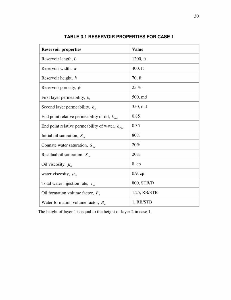
TABLE 3.1 RESERVOIR PROPERTIES FOR CASE 1
Reservoir properties Value
Reservoir length, L 1200, ft
Reservoir width, w 400, ft
Reservoir height, h 70, ft
Reservoir porosity, φ 25 %
First layer permeability, 1k 500, md
Second layer permeability, 2k 350, md
End point relative permeability of oil, roek 0.85
End point relative permeability of water, rwek 0.35
Initial oil saturation, oiS 80%
Connate water saturation, wcS 20%
Residual oil saturation, orS 20%
Oil viscosity, oµ 8, cp
water viscosity, wµ 0.9, cp
Total water injection rate, wti 800, STB/D
Oil formation volume factor, oB 1.25, RB/STB
Water formation volume factor, wB 1, RB/STB
The height of layer 1 is equal to the height of layer 2 in case 1.
31 -
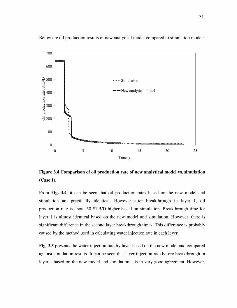
Below are oil production results of new analytical model compared to simulation model:
0
100
200
300
400
500
600
700
0 5 10 15 20 25
Time, yr
Oil
prod
uctio
n ra
te, S
TB
/D Simulation
New analytical model
Figure 3.4 Comparison of oil production rate of new analytical model vs. simulation
(Case 1).
From Fig. 3.4, it can be seen that oil production rates based on the new model and
simulation are practically identical. However after breakthrough in layer 1, oil
production rate is about 50 STB/D higher based on simulation. Breakthrough time for
layer 1 is almost identical based on the new model and simulation. However, there is
significant difference in the second layer breakthrough times. This difference is probably
caused by the method used in calculating water injection rate in each layer.
Fig. 3.5 presents the water injection rate by layer based on the new model and compared
against simulation results. It can be seen that layer injection rate before breakthrough in
layer – based on the new model and simulation – is in very good agreement. However,
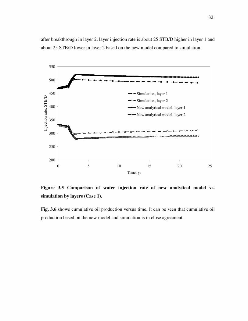
32 -
after breakthrough in layer 2, layer injection rate is about 25 STB/D higher in layer 1 and
about 25 STB/D lower in layer 2 based on the new model compared to simulation.
200
250
300
350
400
450
500
550
0 5 10 15 20 25
Time, yr
Inje
ctio
n ra
te, S
TB
/D
Simulation, layer 1
Simulation, layer 2
New analytical model, layer 1
New analytical model, layer 2
Figure 3.5 Comparison of water injection rate of new analytical model vs.
simulation by layers (Case 1).
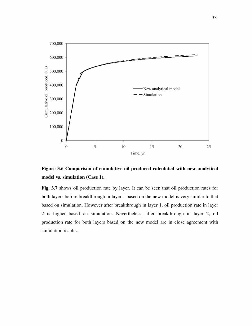
Fig. 3.6 shows cumulative oil production versus time. It can be seen that cumulative oil
production based on the new model and simulation is in close agreement.
33 -
0
100,000
200,000
300,000
400,000
500,000
600,000
700,000
0 5 10 15 20 25
Time, yr
Cum
ulat
ive
oil p
rodu
ced,
ST
B
New analytical modelSimulation
Figure 3.6 Comparison of cumulative oil produced calculated with new analytical
model vs. simulation (Case 1).
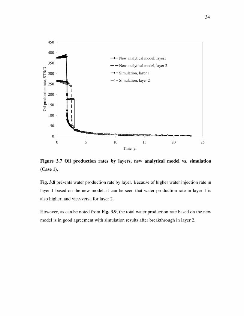
Fig. 3.7 shows oil production rate by layer. It can be seen that oil production rates for
both layers before breakthrough in layer 1 based on the new model is very similar to that
based on simulation. However after breakthrough in layer 1, oil production rate in layer
2 is higher based on simulation. Nevertheless, after breakthrough in layer 2, oil
production rate for both layers based on the new model are in close agreement with
simulation results.
34 -
0
50
100
150
200
250
300
350
400
450
0 5 10 15 20 25
Time, yr
Oil
prod
uctio
n ra
te, S
TB
/D
New analytical model, layer1
New analytical model, layer 2
Simulation, layer 1
Simulation, layer 2
Figure 3.7 Oil production rates by layers, new analytical model vs. simulation
(Case 1).
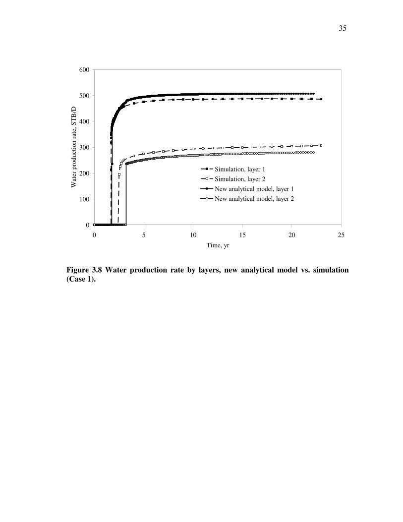
Fig. 3.8 presents water production rate by layer. Because of higher water injection rate in
layer 1 based on the new model, it can be seen that water production rate in layer 1 is
also higher, and vice-versa for layer 2.
However, as can be noted from Fig. 3.9, the total water production rate based on the new
model is in good agreement with simulation results after breakthrough in layer 2.
35 -
0
100
200
300
400
500
600
0 5 10 15 20 25
Time, yr
Wat
er p
rodu
ctio
n ra
te, S
TB
/D
Simulation, layer 1Simulation, layer 2New analytical model, layer 1New analytical model, layer 2
Figure 3.8 Water production rate by layers, new analytical model vs. simulation (Case 1).
36 -
0
100
200
300
400
500
600
700
800
900
0 5 10 15 20 25
Time, yr
Wat
er p
rodu
ctio
n ra
te, S
TB
/D
New analytical modelSimulation
Figure 3.9 Total water production rate comparison of new analytical model vs. simulation (Case 1).
3.3 Case 2
One of the goals of this study was to apply different sets of relative permeability to
different layers and compare calculated results to that of simulation. Case 2 is identical
to Case 1 except the oil-water relative permeability set for layer 2 has been changed as
follows: 2roek is 0.9 and 2rwek is 0.5 fraction, residual oil saturation 2orS is 35 %,
and 2wcS is 20 %. Parameters for Case 2 are shown in Tables 3.2-3.3.
37 -
TABLE 3.2 RESERVOIR PROPERTIES OF LAYER 1 FOR CASE 2.
Layer 1 Characteristics Value
Layer 1 length, L 1200, ft
Layer 1 width, w 400, ft
Layer 1 height, h 35, ft
Layer 1 porosity, φ 25 %
Layer 1 permeability, 1k 500, md
End point relative permeability of oil, roek 0.85
End point relative permeability of water, rwek 0.35
Initial oil saturation, oiS 80%
Connate water saturation, wcS 20%
Residual oil saturation, orS 20%
Oil viscosity, oµ 8, cp
water viscosity, wµ 0.9, cp
water injection rate in layer 1, 1wi variable, STB/D
Oil formation volume factor, oB 1.25, RB/STB
Water formation volume factor, wB 1, RB/STB
38 -
TABLE 3.3 RESERVOIR PROPERTIES OF LAYER 2 FOR CASE 2.
Layer 2 Characteristics Value
Layer 2 length, L 1200, ft
Layer 2 width, w 400, ft
Layer 2 height, h 35, ft
Layer 2 porosity, φ 25 %
Layer 2 permeability, 2k 350, md
End point relative permeability of oil, roek 0.9
End point relative permeability of water, rwek 0.5
Initial oil saturation, oiS 70%
Connate water saturation, wcS 30%
Residual oil saturation, orS 35%
Oil viscosity, oµ 8, cp
water viscosity, wµ 0.9, cp
water injection rate in layer 2, 2wi variable, STB/D
Oil formation volume factor, oB 1.25, RB/STB
Water formation volume factor, wB 1, RB/STB
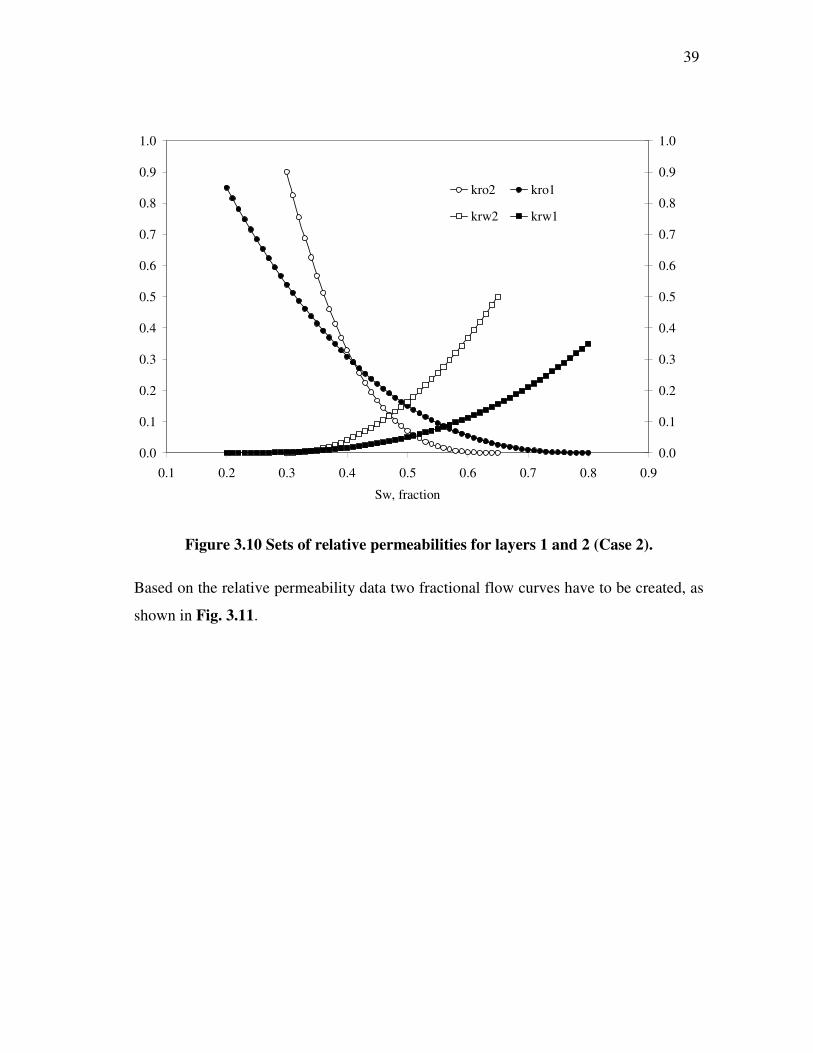
Two sets of oil-water relative permeability are shown in Fig. 3.10.
39 -
0.0
0.1
0.2
0.3
0.4
0.5
0.6
0.7
0.8
0.9
1.0
0.1 0.2 0.3 0.4 0.5 0.6 0.7 0.8 0.9
Sw, fraction
0.0
0.1
0.2
0.3
0.4
0.5
0.6
0.7
0.8
0.9
1.0
kro2 kro1
krw2 krw1
Figure 3.10 Sets of relative permeabilities for layers 1 and 2 (Case 2).
Based on the relative permeability data two fractional flow curves have to be created, as
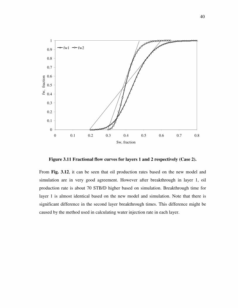
shown in Fig. 3.11.
40 -
0
0.1
0.2
0.3
0.4
0.5
0.6
0.7
0.8
0.9
1
0 0.1 0.2 0.3 0.4 0.5 0.6 0.7 0.8
Sw, fraction
fw,
frac
tion
fw1 fw2
Figure 3.11 Fractional flow curves for layers 1 and 2 respectively (Case 2).
From Fig. 3.12, it can be seen that oil production rates based on the new model and
simulation are in very good agreement. However after breakthrough in layer 1, oil
production rate is about 70 STB/D higher based on simulation. Breakthrough time for
layer 1 is almost identical based on the new model and simulation. Note that there is
significant difference in the second layer breakthrough times. This difference might be
caused by the method used in calculating water injection rate in each layer.

41 -
0
100
200
300
400
500
600
700
0 5 10 15 20 25 30
Time, yr
Oil
prod
uctio
n ra
te, S
TB
/D Simulation
New analytical model
Figure 3.12 Oil production rate of new analytical model vs. simulation, different
sets of relative permeabilities are applied (Case 2).
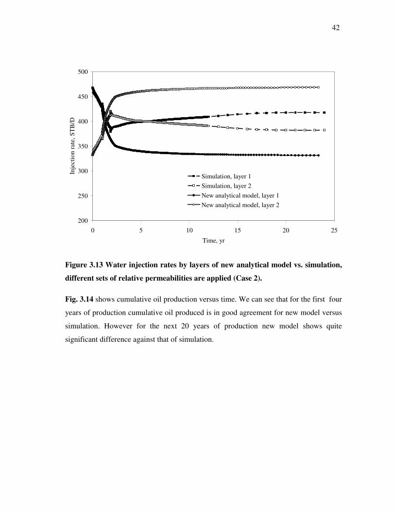
Fig. 3.13 presents the water injection rate by layer based on the new model and
simulation results. It can be noted, that layer injection rate before breakthrough is in very
good agreement. Nevertheless, after breakthrough in layer 2, layer injection rate is about
60 STB/D higher in layer 1, and about 60 STB/D lower in layer 2 according to the new
model compared against simulation.
42 -
200
250
300
350
400
450
500
0 5 10 15 20 25
Time, yr
Inje
ctio
n ra
te, S
TB
/D
Simulation, layer 1Simulation, layer 2New analytical model, layer 1New analytical model, layer 2
Figure 3.13 Water injection rates by layers of new analytical model vs. simulation,
different sets of relative permeabilities are applied (Case 2).
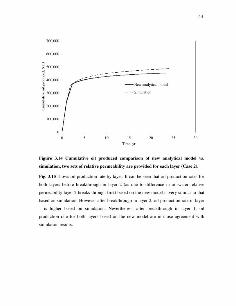
Fig. 3.14 shows cumulative oil production versus time. We can see that for the first four
years of production cumulative oil produced is in good agreement for new model versus
simulation. However for the next 20 years of production new model shows quite
significant difference against that of simulation.
43 -
0
100,000
200,000
300,000
400,000
500,000
600,000
700,000
0 5 10 15 20 25 30
Time, yr
Cum
ulat
ive
oil p
rodu
ced,
ST
B
New analytical model
Simulation
Figure 3.14 Cumulative oil produced comparison of new analytical model vs.
simulation, two sets of relative permeability are provided for each layer (Case 2).
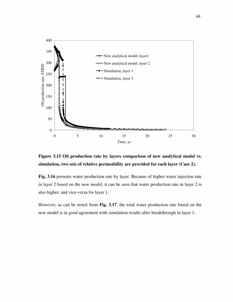
Fig. 3.15 shows oil production rate by layer. It can be seen that oil production rates for
both layers before breakthrough in layer 2 (as due to difference in oil-water relative
permeability layer 2 breaks through first) based on the new model is very similar to that
based on simulation. However after breakthrough in layer 2, oil production rate in layer
1 is higher based on simulation. Nevertheless, after breakthrough in layer 1, oil
production rate for both layers based on the new model are in close agreement with
simulation results.
44 -
0
50
100
150
200
250
300
350
400
0 5 10 15 20 25 30
Time, yr
Oil
prod
uctio
n ra
te, S
TB
/D
New analytical model, layer1
New analytical model, layer 2
Simulation, layer 1
Simulation, layer 2
Figure 3.15 Oil production rate by layers comparison of new analytical model vs.
simulation, two sets of relative permeability are provided for each layer (Case 2).
Fig. 3.16 presents water production rate by layer. Because of higher water injection rate
in layer 2 based on the new model, it can be seen that water production rate in layer 2 is
also higher, and vice-versa for layer 1.
However, as can be noted from Fig. 3.17, the total water production rate based on the
new model is in good agreement with simulation results after breakthrough in layer 1.
45 -
0
50
100
150
200
250
300
350
400
450
500
0 5 10 15 20 25 30Time, yr
Wat
er p
rodu
ctio
n ra
te, S
TB
/D
Simulation, layer 1
Simulation, layer 2
New analytical model, layer 1
New analytical model, layer 2
Figure 3.16 Water production rate by layers, comparison of new analytical model
vs. simulation, two sets of relative permeability are provided for each layer (Case2).
46 -
0
100
200
300
400
500
600
700
800
900
0 5 10 15 20 25 30
Time, yr
Wat
er p
rodu
ctio
n ra
te, S
TB
/D
New analytical modelSimulation
Figure 3.17 Total water production rate, comparison of new analytical model vs.
simulation, two sets of relative permeability are provided for each layer (Case 2).
3.4 Case 3
Next case represents the variation of the case 1 with different set of kh . Table 3.4
contains the changes made to the model:
47 -
TABLE 3.4 HEIGHT AND PERMEABILITY VARIATION IN LAYERS 1 AND 2.
Characteristics Value
Absolute permeability of layer 1, 1k 500, md
Height of layer 1, 1h 50, ft
Absolute permeability of layer 2, 2k 100, md
Height of layer 2, 2h 25, ft
From Fig. 3.18, it can be seen that oil production rates based on the new model and
simulation are in good agreement. However after breakthrough in layer 1, oil production
rate is about 30 STB/D lower based on simulation. Breakthrough time for layer 1 is very
close based on the new model and simulation. Note that there is significant difference of
2.5 years in the second layer breakthrough times. This difference is probably caused by
the method used in calculating water injection rate in each layer.
48 -
0
100
200
300
400
500
600
700
0 5 10 15 20 25
Time, yr
Oil
prod
uctio
n ra
te, S
TB
/D Simulation
New analytical model
Figure 3.18 Oil production comparison of new analytical model to the simulation,
variable kh is applied (Case 3).
Fig. 3.19 presents the water injection rate by layer based on the new model and
simulation results. It can be noted, that there is constant difference of 30 STB/D in layer
injection rate before and after breakthrough.
49 -
0
100
200
300
400
500
600
700
800
0 5 10 15 20 25
Time, yr
Inje
ctio
n ra
te, S
TB
/D
Simulation, layer 1
Simulation, layer 2
New analytical model, layer 1
New analytical model, layer 2
Figure 3.19 Water injection rate comparison of new analytical model versus
simulation, variable kh is applied (Case 3).
Fig. 3.20 shows cumulative oil production versus time. We can see that overall
cumulative oil production is in good agreement for new model versus simulation.
However for period of time from 2nd year of production to 10th year there is significant
difference of new model against that of simulation.

50 -
0
100,000
200,000
300,000
400,000
500,000
600,000
700,000
0 5 10 15 20 25
Time, yr
Cum
ulat
ive
oil p
rodu
ced,
ST
B
New analytical modelSimulation
Figure 3.20 Cumulative oil produced comparison of new analytical model to the
simulation, variable kh is applied (Case 3).
Fig. 3.21 shows oil production rate by layer. It can be seen that oil production rate for
both layers before breakthrough in layer 1 based on the new model gives a difference of
30 STB/D to that based on simulation, where simulation production rate is higher.
However after breakthrough in layer 2, oil production rate in layer 2 is higher based on
new model. Nevertheless, after breakthrough in layer 1, oil production rate for both
layers based on the new model are in close agreement with simulation results.
51 -
0
100
200
300
400
500
600
700
0 5 10 15 20 25
Time, yr
Oil
prod
uctio
n ra
te, S
TB
/D
New analytical model, layer1
New analytical model, layer 2
Simulation, layer 1
Simulation, layer 2
Figure 3.21 Oil production layer by layer comparison of new analytical model to
the simulation, variable kh is applied (Case 3).
Fig. 3.22 presents water production rate by layer. Because of higher water injection rate
in layer 1 based on the simulation, it can be seen that water production rate in layer 1 is
also higher, and vice-versa for layer 2.
However, as can be noted from Fig. 3.23, the total water production rate based on the
new model is in close agreement with simulation results after breakthrough in layer 2
based on the simulation.
52 -
0
100
200
300
400
500
600
700
800
0 5 10 15 20 25
Time, yr
Wat
er p
rodu
ctio
n ra
te, S
TB
/D
1-D Simulation layer 1
1-D Simulation layer 2
New analytical model, layer 1
New analytical model, layer 2
Figure 3.22 Water production layer by layer comparison of new analytical model to
the simulation, variable kh is applied (Case 3).
53 -
0
100
200
300
400
500
600
700
800
900
0 5 10 15 20 25
Time, yr
Wat
er p
rodu
ctio
n ra
te, S
TB
/D
New analytical modelSimulation
Figure 3.23 Total water production comparison of new analytical model to the
simulation, variable kh is applied.
3.5 Case 4
Case 4 is obtained by using kh parameters of Case 3 applied to the different oil-water
relative permeability set of Case 2.
From Fig. 3.24, it can be noted that oil production rates based on the new model and
simulation are in good agreement. However after breakthrough in layer 1, oil production
rate is about 50 STB/D higher based on simulation. Breakthrough time for layer 1 is very
close based on the new model and simulation. Note that there is significant difference in
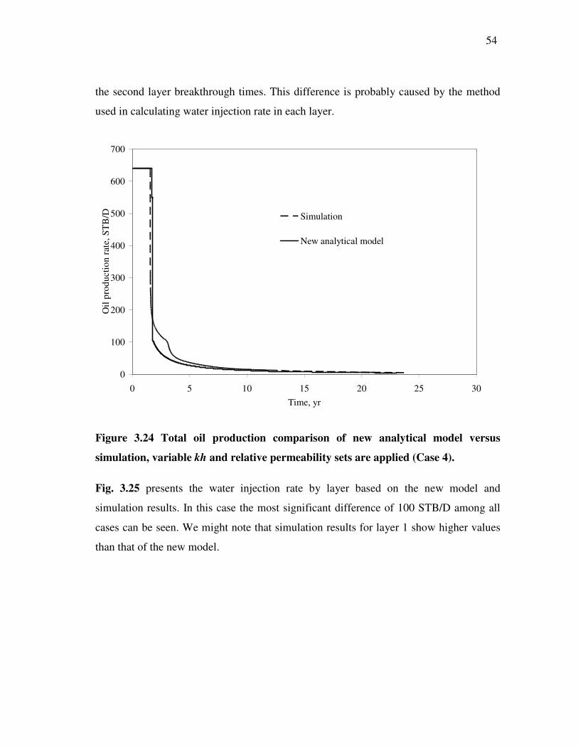
54 -
the second layer breakthrough times. This difference is probably caused by the method
used in calculating water injection rate in each layer.
0
100
200
300
400
500
600
700
0 5 10 15 20 25 30Time, yr
Oil
prod
uctio
n ra
te, S
TB
/D Simulation
New analytical model
Figure 3.24 Total oil production comparison of new analytical model versus
simulation, variable kh and relative permeability sets are applied (Case 4).
Fig. 3.25 presents the water injection rate by layer based on the new model and
simulation results. In this case the most significant difference of 100 STB/D among all
cases can be seen. We might note that simulation results for layer 1 show higher values
than that of the new model.
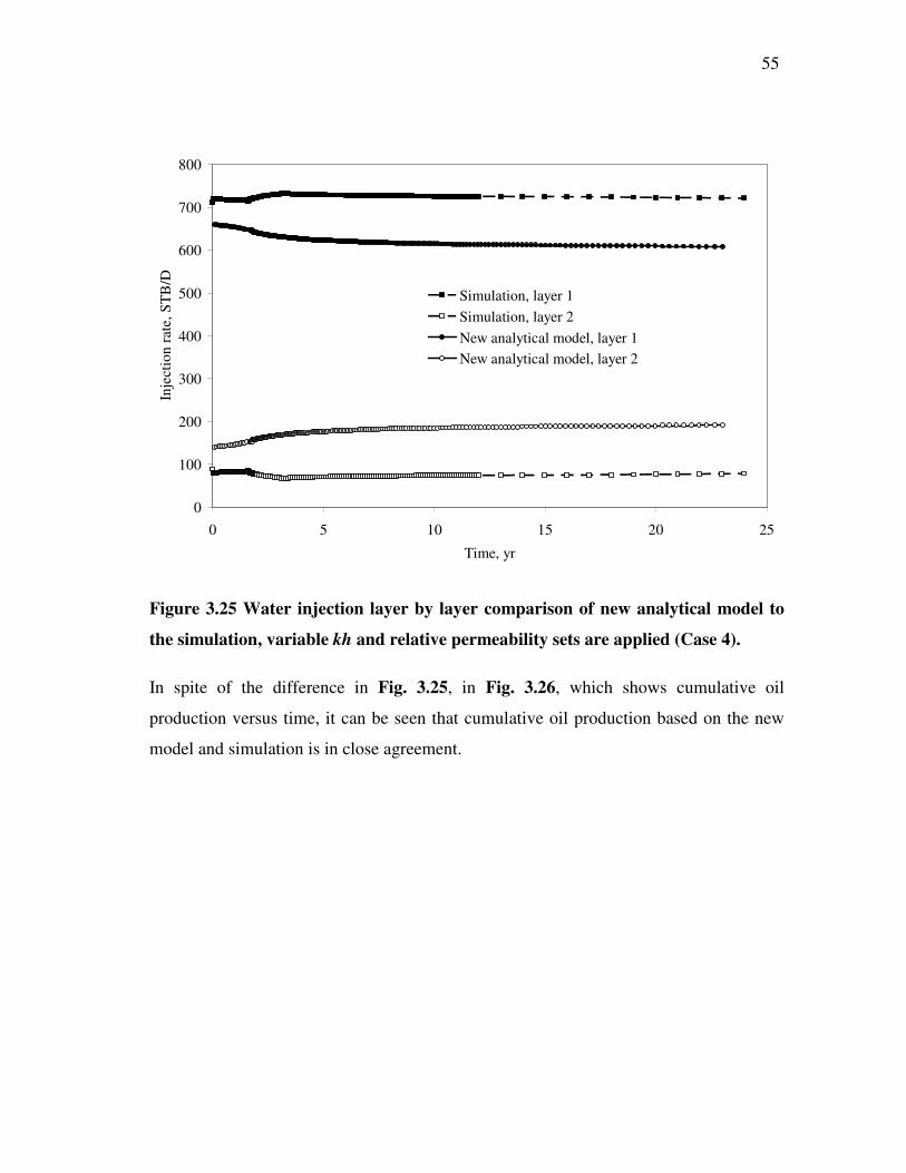
55 -
0
100
200
300
400
500
600
700
800
0 5 10 15 20 25
Time, yr
Inje
ctio
n ra
te, S
TB
/D
Simulation, layer 1Simulation, layer 2New analytical model, layer 1New analytical model, layer 2
Figure 3.25 Water injection layer by layer comparison of new analytical model to
the simulation, variable kh and relative permeability sets are applied (Case 4).
In spite of the difference in Fig. 3.25, in Fig. 3.26, which shows cumulative oil
production versus time, it can be seen that cumulative oil production based on the new
model and simulation is in close agreement.

56 -
0
100,000
200,000
300,000
400,000
500,000
600,000
700,000
0 5 10 15 20 25 30Time, yr
Cum
ulat
ive
oil p
rodu
ced,
ST
B
New analytical model
Simulation
Figure 3.26 Cumulative oil produced, comparison of new analytical model to
simulation, variable kh and relative permeability sets are applied (Case 4).
Fig. 3.27 shows oil production rate by layer. It can be seen that oil production rate for
both layers before breakthrough in layer 1 based on the new model gives a significant
difference of 70 STB/D to that based on simulation, where simulation production rate is
higher for layer 1. However after breakthrough in layer 2, oil production rate in layer 2 is
higher based on new model. However, after breakthrough in layer 1, oil production rate
for both layers based on the new model are in close agreement with simulation results.
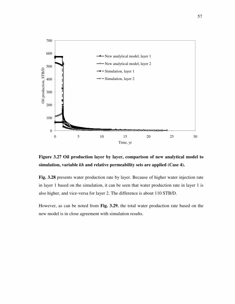
57 -
0
100
200
300
400
500
600
700
0 5 10 15 20 25 30
Time, yr
Oil
prod
uctio
n, S
TB
/D
New analytical model, layer 1
New analytical model, layer 2
Simulation, layer 1
Simulation, layer 2
Figure 3.27 Oil production layer by layer, comparison of new analytical model to
simulation, variable kh and relative permeability sets are applied (Case 4).
Fig. 3.28 presents water production rate by layer. Because of higher water injection rate
in layer 1 based on the simulation, it can be seen that water production rate in layer 1 is
also higher, and vice-versa for layer 2. The difference is about 110 STB/D.
However, as can be noted from Fig. 3.29, the total water production rate based on the
new model is in close agreement with simulation results.
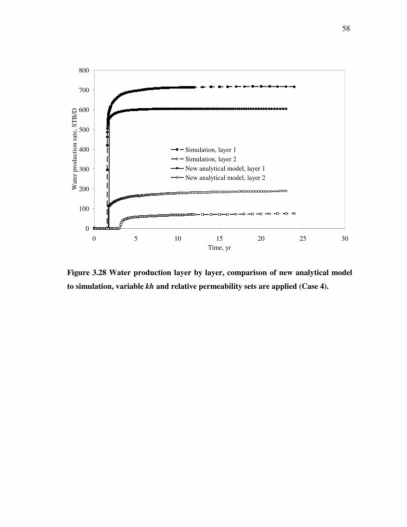
58 -
0
100
200
300
400
500
600
700
800
0 5 10 15 20 25 30Time, yr
Wat
er p
rodu
ctio
n ra
te, S
TB
/D
Simulation, layer 1Simulation, layer 2New analytical model, layer 1New analytical model, layer 2
Figure 3.28 Water production layer by layer, comparison of new analytical model
to simulation, variable kh and relative permeability sets are applied (Case 4).
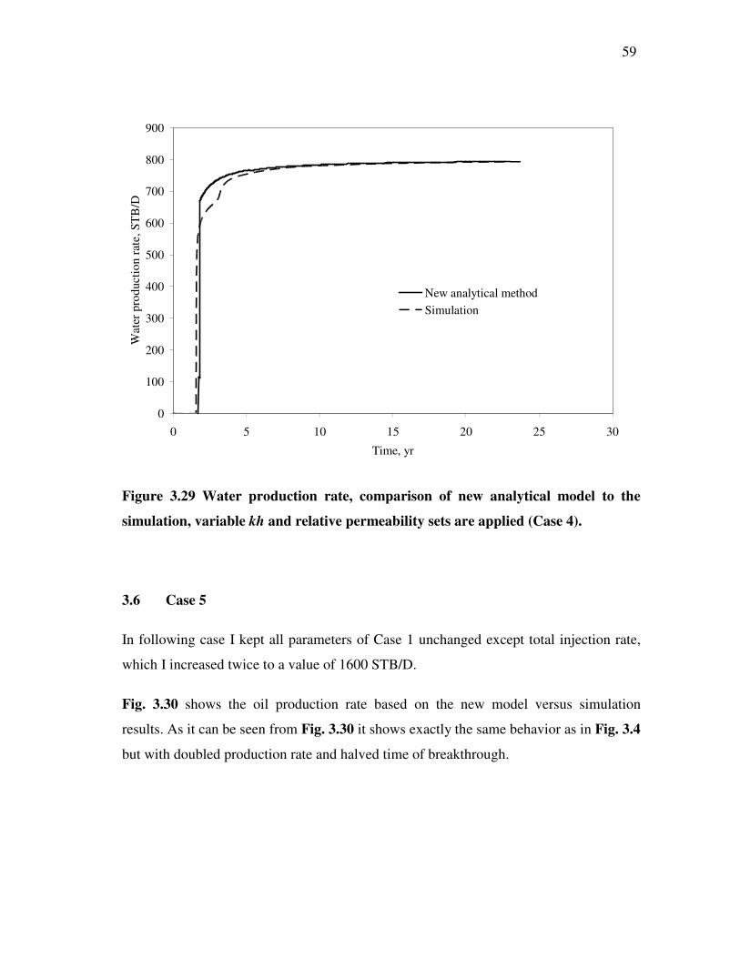
59 -
0
100
200
300
400
500
600
700
800
900
0 5 10 15 20 25 30
Time, yr
Wat
er p
rodu
ctio
n ra
te, S
TB
/D
New analytical methodSimulation
Figure 3.29 Water production rate, comparison of new analytical model to the
simulation, variable kh and relative permeability sets are applied (Case 4).
3.6 Case 5
In following case I kept all parameters of Case 1 unchanged except total injection rate,
which I increased twice to a value of 1600 STB/D.
Fig. 3.30 shows the oil production rate based on the new model versus simulation
results. As it can be seen from Fig. 3.30 it shows exactly the same behavior as in Fig. 3.4
but with doubled production rate and halved time of breakthrough.
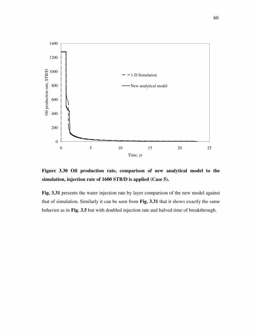
60 -
0
200
400
600
800
1000
1200
1400
0 5 10 15 20 25
Time, yr
Oil
prod
uctio
n ra
te, S
TB
/D
1-D Simulation
New analytical model
Figure 3.30 Oil production rate, comparison of new analytical model to the
simulation, injection rate of 1600 STB/D is applied (Case 5).
Fig. 3.31 presents the water injection rate by layer comparison of the new model against
that of simulation. Similarly it can be seen from Fig. 3.31 that it shows exactly the same
behavior as in Fig. 3.5 but with doubled injection rate and halved time of breakthrough.
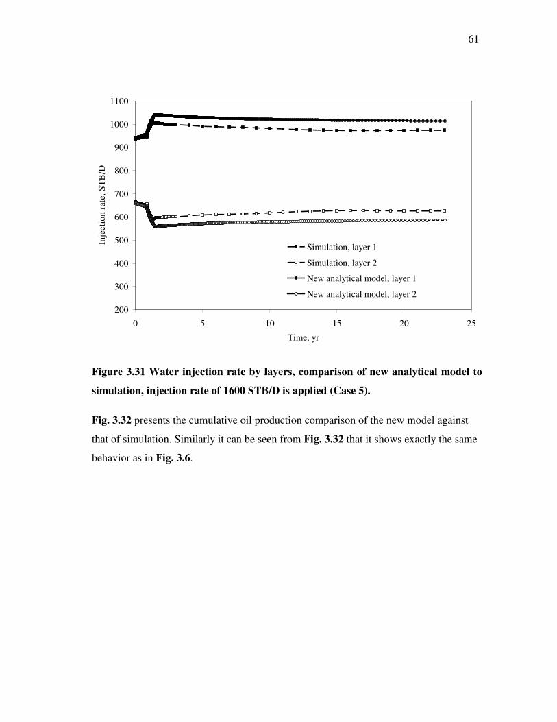
61 -
200
300
400
500
600
700
800
900
1000
1100
0 5 10 15 20 25
Time, yr
Inje
ctio
n ra
te, S
TB
/D
Simulation, layer 1
Simulation, layer 2
New analytical model, layer 1
New analytical model, layer 2
Figure 3.31 Water injection rate by layers, comparison of new analytical model to
simulation, injection rate of 1600 STB/D is applied (Case 5).
Fig. 3.32 presents the cumulative oil production comparison of the new model against
that of simulation. Similarly it can be seen from Fig. 3.32 that it shows exactly the same
behavior as in Fig. 3.6.

62 -
0
100,000
200,000
300,000
400,000
500,000
600,000
700,000
0 5 10 15 20 25
Time, yr
Cum
ulat
ive
oil p
rodu
ced,
ST
B
New analytical modelSimulation
Figure 3.32 Cumulative oil production, comparison of new analytical model to
simulation, injection rate of 1600 STB/D is applied (Case 5).
Fig. 3.33 shows oil production rate by layer. It can be seen that oil production rates for
both layers before breakthrough in layer 1 based on the new model is very similar to that
based on simulation. However after breakthrough in layer 1, oil production rate in layer
2 is higher based on simulation. Nevertheless, after breakthrough in layer 2, oil
production rate for both layers based on the new model are in close agreement with
simulation results. Fig. 3.33 is similar to Fig. 3.7.
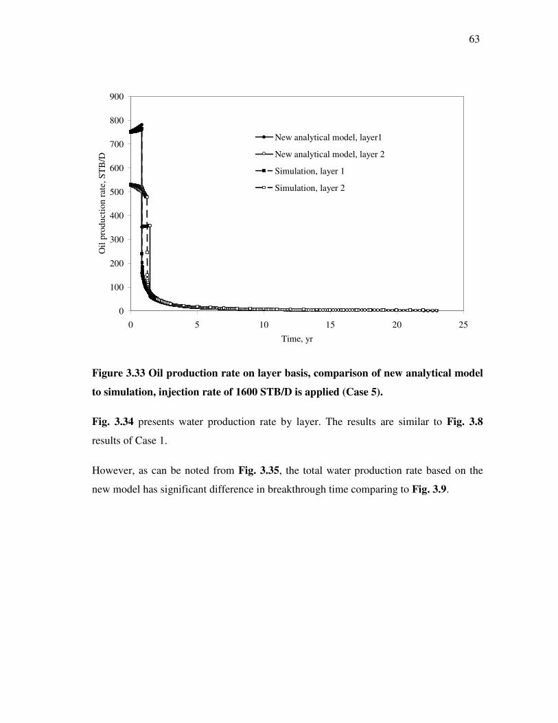
63 -
0
100
200
300
400
500
600
700
800
900
0 5 10 15 20 25
Time, yr
Oil
prod
uctio
n ra
te, S
TB
/D
New analytical model, layer1
New analytical model, layer 2
Simulation, layer 1
Simulation, layer 2
Figure 3.33 Oil production rate on layer basis, comparison of new analytical model
to simulation, injection rate of 1600 STB/D is applied (Case 5).
Fig. 3.34 presents water production rate by layer. The results are similar to Fig. 3.8
results of Case 1.
However, as can be noted from Fig. 3.35, the total water production rate based on the
new model has significant difference in breakthrough time comparing to Fig. 3.9.
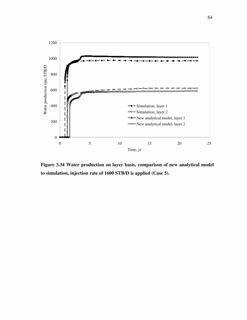
64 -
0
200
400
600
800
1000
1200
0 5 10 15 20 25
Time, yr
Wat
er p
rodu
ctio
n ra
te, S
TB
/D
Simulation, layer 1Simulation, layer 2New analytical model, layer 1New analytical model, layer 2
Figure 3.34 Water production on layer basis, comparison of new analytical model
to simulation, injection rate of 1600 STB/D is applied (Case 5).
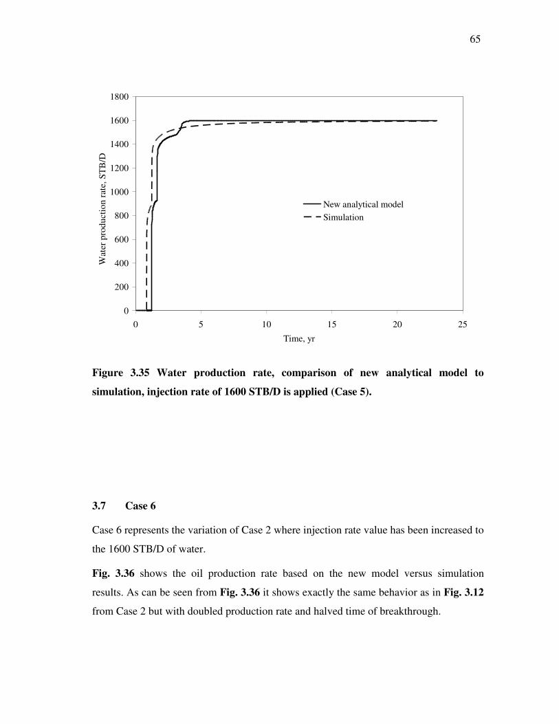
65 -
0
200
400
600
800
1000
1200
1400
1600
1800
0 5 10 15 20 25
Time, yr
Wat
er p
rodu
ctio
n ra
te, S
TB
/D
New analytical modelSimulation
Figure 3.35 Water production rate, comparison of new analytical model to
simulation, injection rate of 1600 STB/D is applied (Case 5).
3.7 Case 6
Case 6 represents the variation of Case 2 where injection rate value has been increased to
the 1600 STB/D of water.
Fig. 3.36 shows the oil production rate based on the new model versus simulation
results. As can be seen from Fig. 3.36 it shows exactly the same behavior as in Fig. 3.12
from Case 2 but with doubled production rate and halved time of breakthrough.
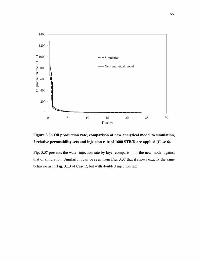
66 -
0
200
400
600
800
1000
1200
1400
0 5 10 15 20 25 30Time, yr
Oil
prod
uctio
n ra
te, S
TB
/D Simulation
New analytical model
Figure 3.36 Oil production rate, comparison of new analytical model to simulation,
2 relative permeability sets and injection rate of 1600 STB/D are applied (Case 6).
Fig. 3.37 presents the water injection rate by layer comparison of the new model against
that of simulation. Similarly it can be seen from Fig. 3.37 that it shows exactly the same
behavior as in Fig. 3.13 of Case 2, but with doubled injection rate.
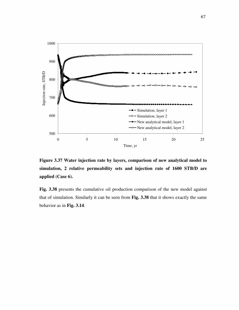
67 -
500
600
700
800
900
1000
0 5 10 15 20 25
Time, yr
Inje
ctio
n ra
te, S
TB
/D
Simulation, layer 1Simulation, layer 2New analytical model, layer 1New analytical model, layer 2
Figure 3.37 Water injection rate by layers, comparison of new analytical model to
simulation, 2 relative permeability sets and injection rate of 1600 STB/D are
applied (Case 6).
Fig. 3.38 presents the cumulative oil production comparison of the new model against
that of simulation. Similarly it can be seen from Fig. 3.38 that it shows exactly the same
behavior as in Fig. 3.14.
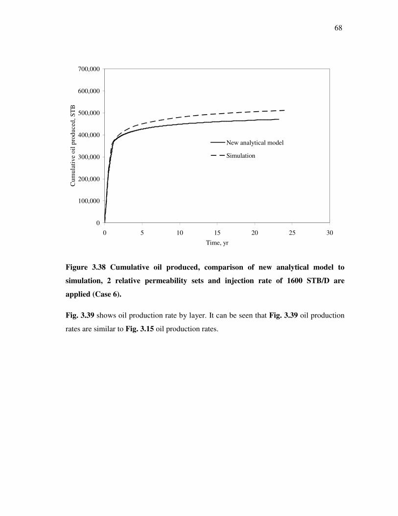
68 -
0
100,000
200,000
300,000
400,000
500,000
600,000
700,000
0 5 10 15 20 25 30Time, yr
Cum
ulat
ive
oil p
rodu
ced,
ST
B
New analytical model
Simulation
Figure 3.38 Cumulative oil produced, comparison of new analytical model to
simulation, 2 relative permeability sets and injection rate of 1600 STB/D are
applied (Case 6).
Fig. 3.39 shows oil production rate by layer. It can be seen that Fig. 3.39 oil production
rates are similar to Fig. 3.15 oil production rates.
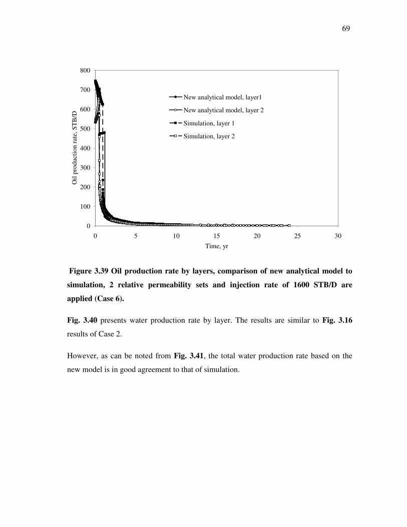
69 -
0
100
200
300
400
500
600
700
800
0 5 10 15 20 25 30
Time, yr
Oil
prod
uctio
n ra
te, S
TB
/D
New analytical model, layer1
New analytical model, layer 2
Simulation, layer 1
Simulation, layer 2
Figure 3.39 Oil production rate by layers, comparison of new analytical model to
simulation, 2 relative permeability sets and injection rate of 1600 STB/D are
applied (Case 6).
Fig. 3.40 presents water production rate by layer. The results are similar to Fig. 3.16
results of Case 2.
However, as can be noted from Fig. 3.41, the total water production rate based on the
new model is in good agreement to that of simulation.

70 -
0
100
200
300
400
500
600
700
800
900
1000
0 5 10 15 20 25 30Time, yr
Wat
er p
rodu
ctio
n ra
te, S
TB
/D
Simulation, layer 1
Simulation, layer 2
New analytical model, layer 1
New analytical model, layer 2
Figure 3.40 Water production rate by layers, comparison of new analytical model
to simulation, 2 relative permeability sets and injection rate of 1600 STB/D are
applied (Case 6).
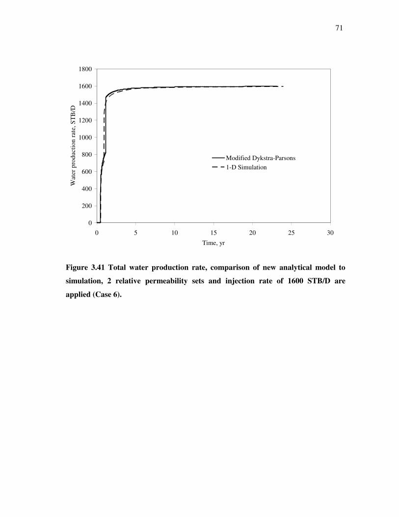
71 -
0
200
400
600
800
1000
1200
1400
1600
1800
0 5 10 15 20 25 30
Time, yr
Wat
er p
rodu
ctio
n ra
te, S
TB
/D
Modified Dykstra-Parsons1-D Simulation
Figure 3.41 Total water production rate, comparison of new analytical model to
simulation, 2 relative permeability sets and injection rate of 1600 STB/D are
applied (Case 6).
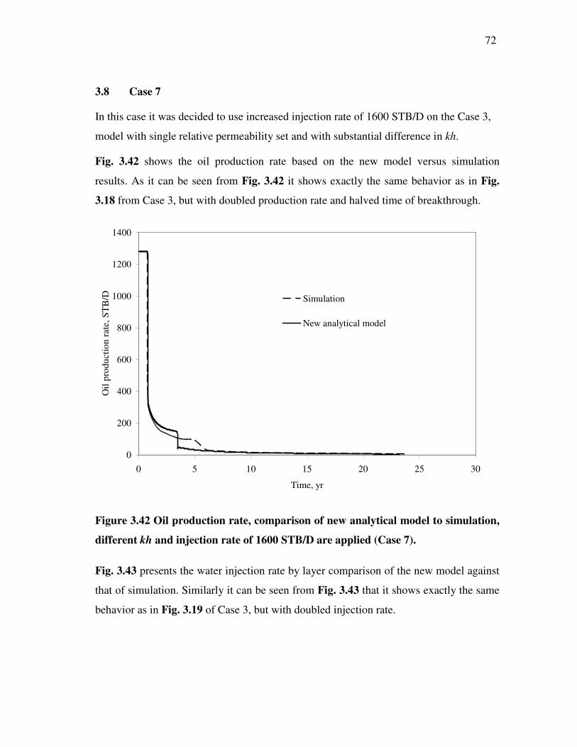
72 -
3.8 Case 7
In this case it was decided to use increased injection rate of 1600 STB/D on the Case 3,
model with single relative permeability set and with substantial difference in kh.
Fig. 3.42 shows the oil production rate based on the new model versus simulation
results. As it can be seen from Fig. 3.42 it shows exactly the same behavior as in Fig.
3.18 from Case 3, but with doubled production rate and halved time of breakthrough.
0
200
400
600
800
1000
1200
1400
0 5 10 15 20 25 30
Time, yr
Oil
prod
uctio
n ra
te, S
TB
/D Simulation
New analytical model
Figure 3.42 Oil production rate, comparison of new analytical model to simulation,
different kh and injection rate of 1600 STB/D are applied (Case 7).
Fig. 3.43 presents the water injection rate by layer comparison of the new model against
that of simulation. Similarly it can be seen from Fig. 3.43 that it shows exactly the same
behavior as in Fig. 3.19 of Case 3, but with doubled injection rate.
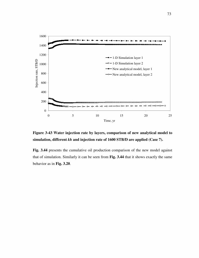
73 -
0
200
400
600
800
1000
1200
1400
1600
0 5 10 15 20 25
Time, yr
Inje
ctio
n ra
te, S
TB/D
1-D Simulation layer 1
1-D Simulation layer 2
New analytical model, layer 1
New analytical model, layer 2
Figure 3-43 Water injection rate by layers, comparison of new analytical model to
simulation, different kh and injection rate of 1600 STB/D are applied (Case 7).
Fig. 3.44 presents the cumulative oil production comparison of the new model against
that of simulation. Similarly it can be seen from Fig. 3.44 that it shows exactly the same
behavior as in Fig. 3.20.
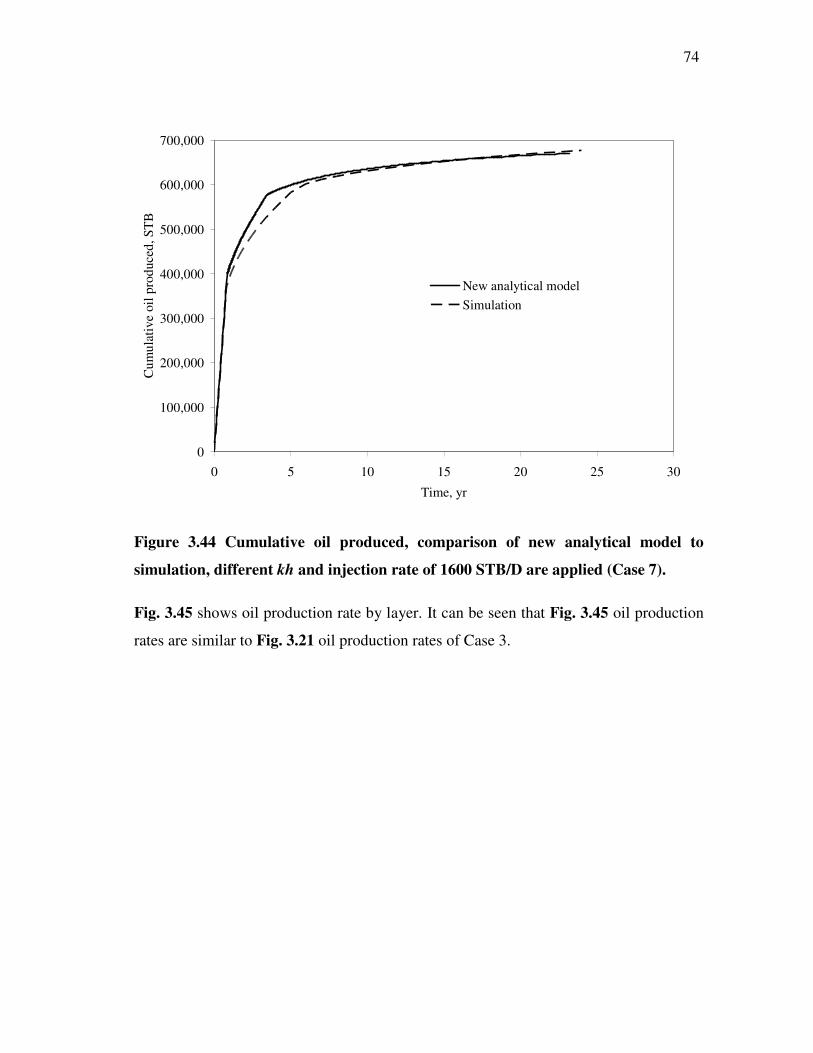
74 -
0
100,000
200,000
300,000
400,000
500,000
600,000
700,000
0 5 10 15 20 25 30
Time, yr
Cum
ulat
ive
oil p
rodu
ced,
ST
B
New analytical modelSimulation
Figure 3.44 Cumulative oil produced, comparison of new analytical model to
simulation, different kh and injection rate of 1600 STB/D are applied (Case 7).
Fig. 3.45 shows oil production rate by layer. It can be seen that Fig. 3.45 oil production
rates are similar to Fig. 3.21 oil production rates of Case 3.
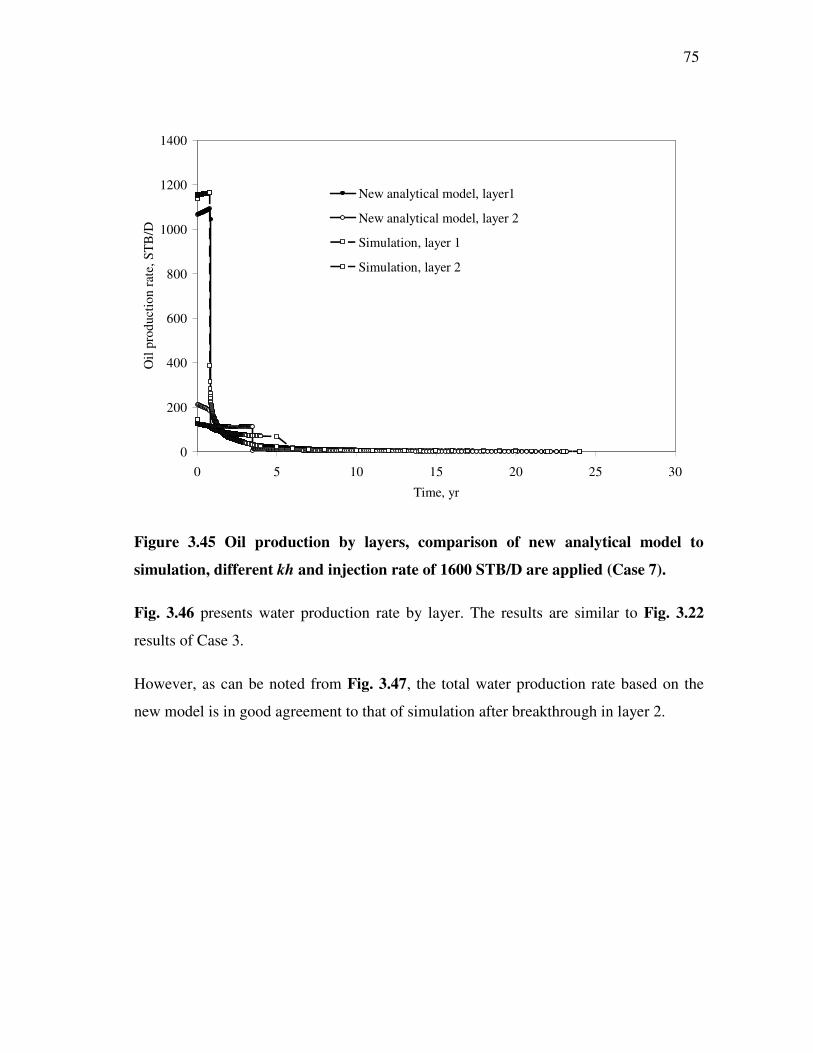
75 -
0
200
400
600
800
1000
1200
1400
0 5 10 15 20 25 30
Time, yr
Oil
prod
uctio
n ra
te, S
TB
/D
New analytical model, layer1
New analytical model, layer 2
Simulation, layer 1
Simulation, layer 2
Figure 3.45 Oil production by layers, comparison of new analytical model to
simulation, different kh and injection rate of 1600 STB/D are applied (Case 7).
Fig. 3.46 presents water production rate by layer. The results are similar to Fig. 3.22
results of Case 3.
However, as can be noted from Fig. 3.47, the total water production rate based on the
new model is in good agreement to that of simulation after breakthrough in layer 2.
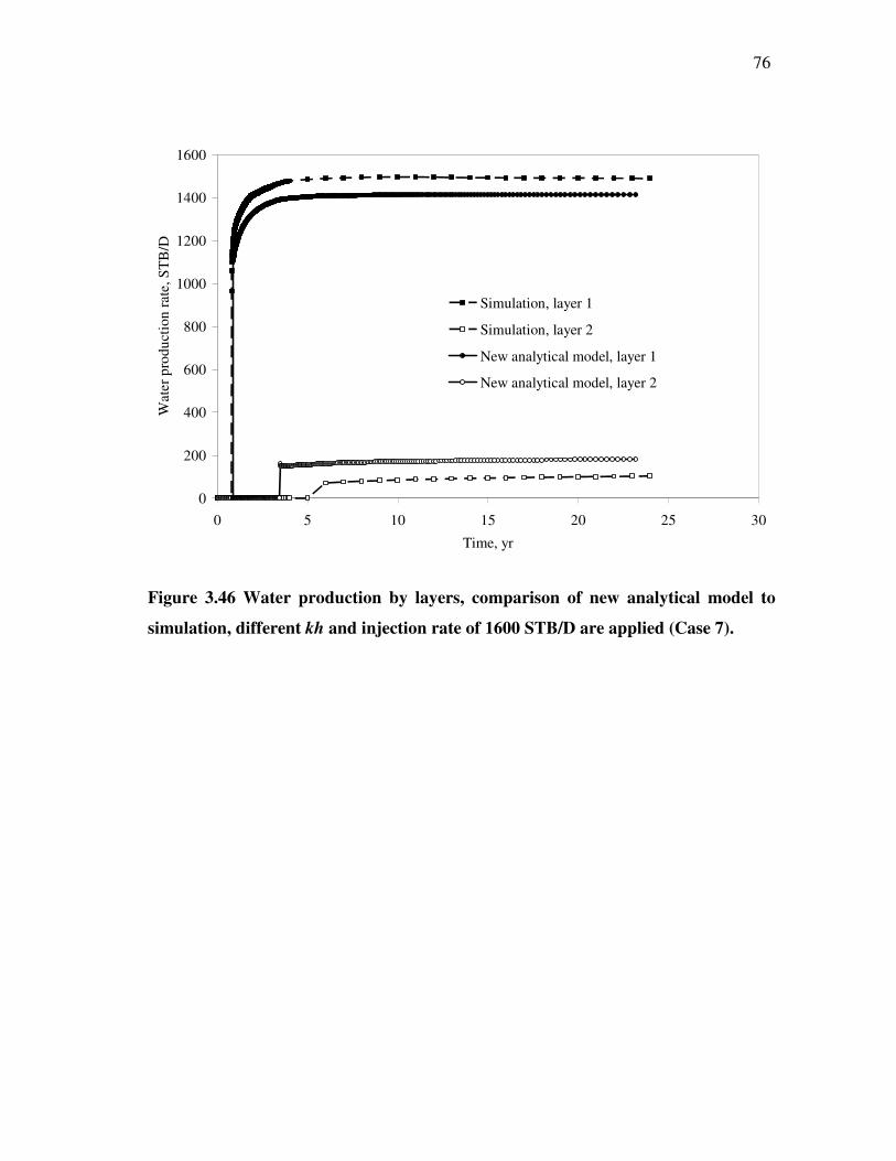
76 -
0
200
400
600
800
1000
1200
1400
1600
0 5 10 15 20 25 30
Time, yr
Wat
er p
rodu
ctio
n ra
te, S
TB
/D
Simulation, layer 1
Simulation, layer 2
New analytical model, layer 1
New analytical model, layer 2
Figure 3.46 Water production by layers, comparison of new analytical model to
simulation, different kh and injection rate of 1600 STB/D are applied (Case 7).
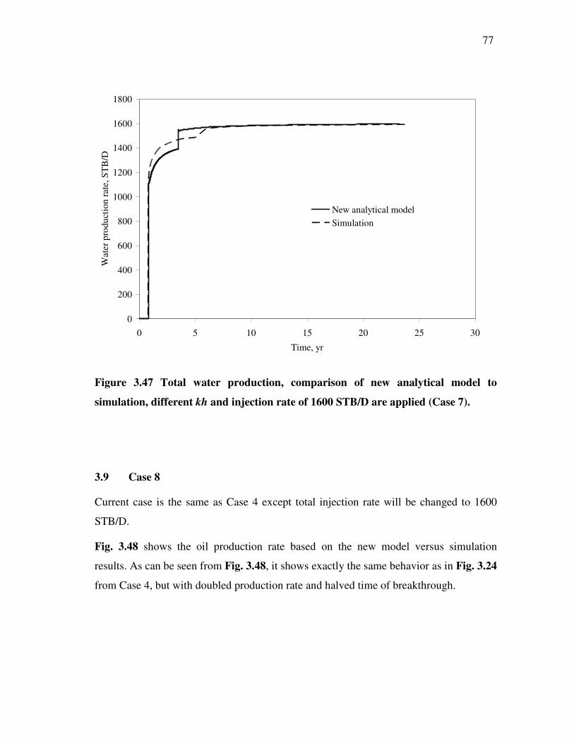
77 -
0
200
400
600
800
1000
1200
1400
1600
1800
0 5 10 15 20 25 30
Time, yr
Wat
er p
rodu
ctio
n ra
te, S
TB
/D
New analytical modelSimulation
Figure 3.47 Total water production, comparison of new analytical model to
simulation, different kh and injection rate of 1600 STB/D are applied (Case 7).
3.9 Case 8
Current case is the same as Case 4 except total injection rate will be changed to 1600
STB/D.
Fig. 3.48 shows the oil production rate based on the new model versus simulation
results. As can be seen from Fig. 3.48, it shows exactly the same behavior as in Fig. 3.24
from Case 4, but with doubled production rate and halved time of breakthrough.
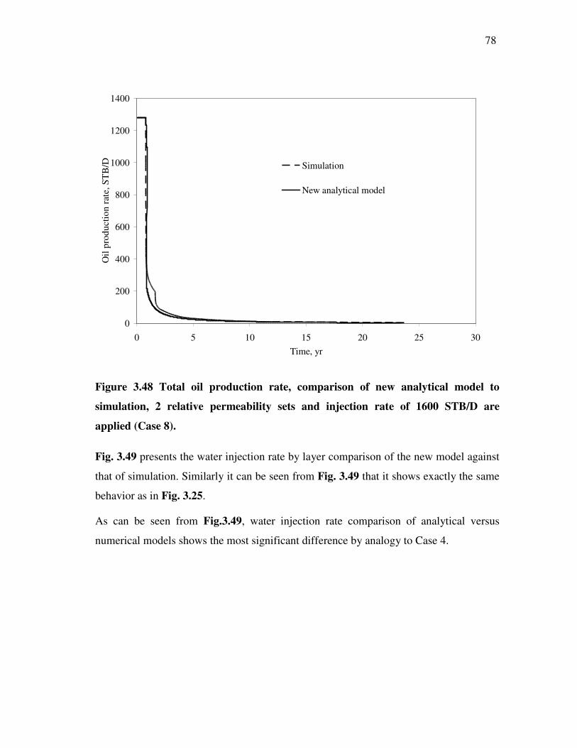
78 -
0
200
400
600
800
1000
1200
1400
0 5 10 15 20 25 30Time, yr
Oil
prod
uctio
n ra
te, S
TB
/D Simulation
New analytical model
Figure 3.48 Total oil production rate, comparison of new analytical model to
simulation, 2 relative permeability sets and injection rate of 1600 STB/D are
applied (Case 8).
Fig. 3.49 presents the water injection rate by layer comparison of the new model against
that of simulation. Similarly it can be seen from Fig. 3.49 that it shows exactly the same
behavior as in Fig. 3.25.
As can be seen from Fig.3.49, water injection rate comparison of analytical versus
numerical models shows the most significant difference by analogy to Case 4.
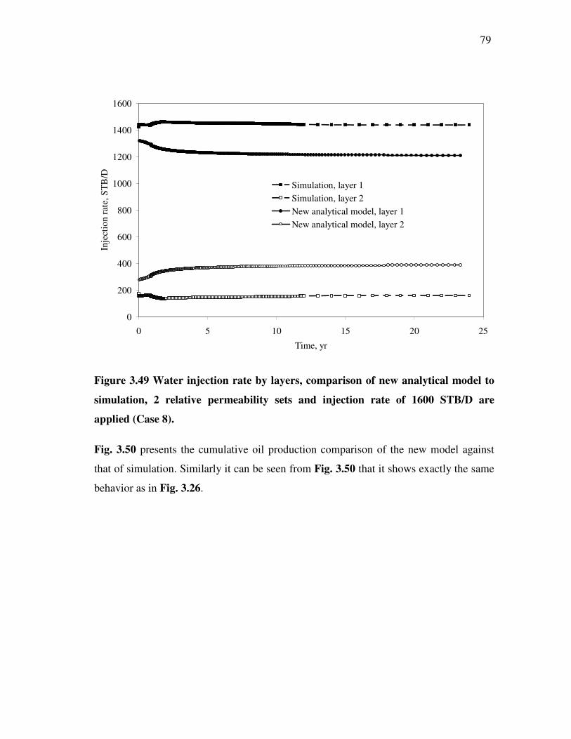
79 -
0
200
400
600
800
1000
1200
1400
1600
0 5 10 15 20 25
Time, yr
Inje
ctio
n ra
te, S
TB
/D
Simulation, layer 1Simulation, layer 2New analytical model, layer 1New analytical model, layer 2
Figure 3.49 Water injection rate by layers, comparison of new analytical model to
simulation, 2 relative permeability sets and injection rate of 1600 STB/D are
applied (Case 8).
Fig. 3.50 presents the cumulative oil production comparison of the new model against
that of simulation. Similarly it can be seen from Fig. 3.50 that it shows exactly the same
behavior as in Fig. 3.26.
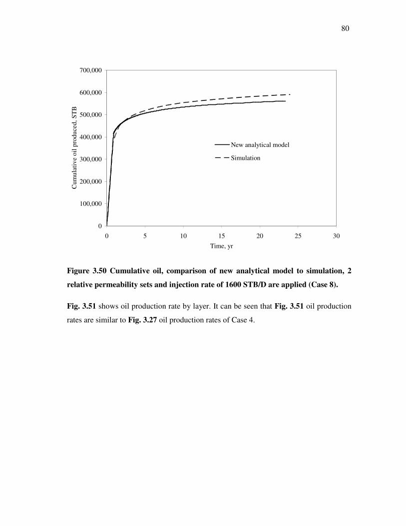
80 -
0
100,000
200,000
300,000
400,000
500,000
600,000
700,000
0 5 10 15 20 25 30Time, yr
Cum
ulat
ive
oil p
rodu
ced,
ST
B
New analytical model
Simulation
Figure 3.50 Cumulative oil, comparison of new analytical model to simulation, 2
relative permeability sets and injection rate of 1600 STB/D are applied (Case 8).
Fig. 3.51 shows oil production rate by layer. It can be seen that Fig. 3.51 oil production
rates are similar to Fig. 3.27 oil production rates of Case 4.
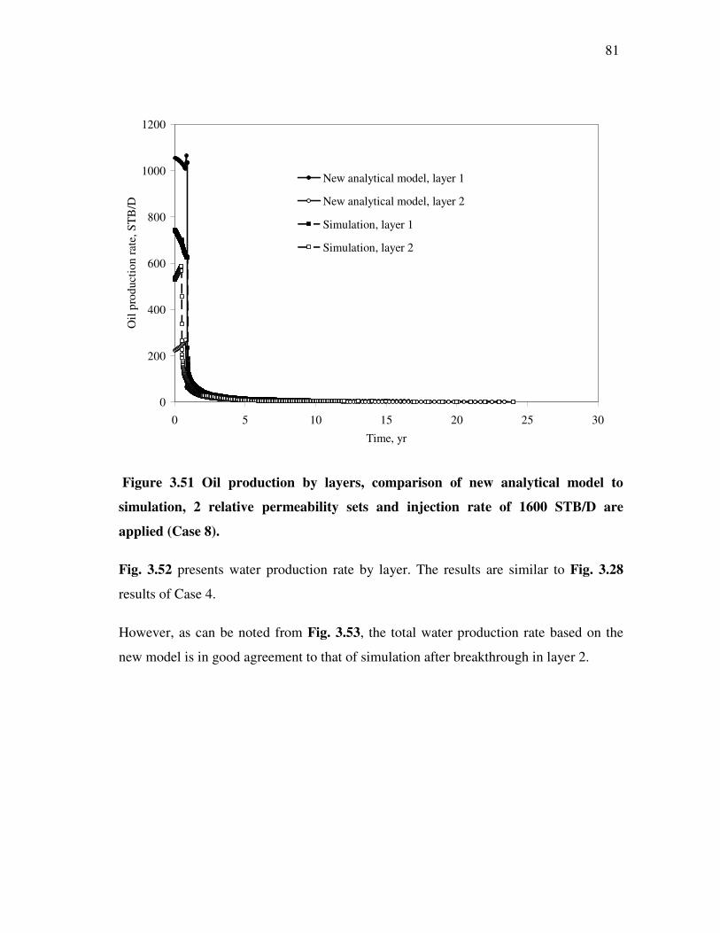
81 -
0
200
400
600
800
1000
1200
0 5 10 15 20 25 30
Time, yr
Oil
prod
uctio
n ra
te, S
TB
/D
New analytical model, layer 1
New analytical model, layer 2
Simulation, layer 1
Simulation, layer 2
Figure 3.51 Oil production by layers, comparison of new analytical model to
simulation, 2 relative permeability sets and injection rate of 1600 STB/D are
applied (Case 8).
Fig. 3.52 presents water production rate by layer. The results are similar to Fig. 3.28
results of Case 4.
However, as can be noted from Fig. 3.53, the total water production rate based on the
new model is in good agreement to that of simulation after breakthrough in layer 2.
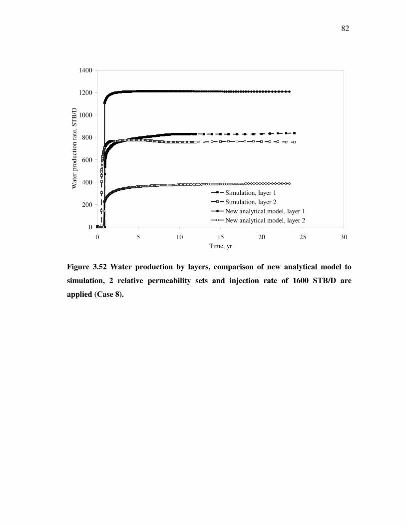
82 -
0
200
400
600
800
1000
1200
1400
0 5 10 15 20 25 30Time, yr
Wat
er p
rodu
ctio
n ra
te, S
TB
/D
Simulation, layer 1Simulation, layer 2New analytical model, layer 1New analytical model, layer 2
Figure 3.52 Water production by layers, comparison of new analytical model to
simulation, 2 relative permeability sets and injection rate of 1600 STB/D are
applied (Case 8).
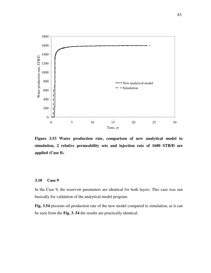
83 -
0
200
400
600
800
1000
1200
1400
1600
1800
0 5 10 15 20 25 30
Time, yr
Wat
er p
rodu
ctio
n ra
te, S
TB
/D
New analytical modelSimulation
Figure 3.53 Water production rate, comparison of new analytical model to
simulation, 2 relative permeability sets and injection rate of 1600 STB/D are
applied (Case 8).
3.10 Case 9
In the Case 9, the reservoir parameters are identical for both layers. This case was run
basically for validation of the analytical model program.
Fig. 3.54 presents oil production rate of the new model compared to simulation, as it can
be seen from the Fig. 3. 54 the results are practically identical.
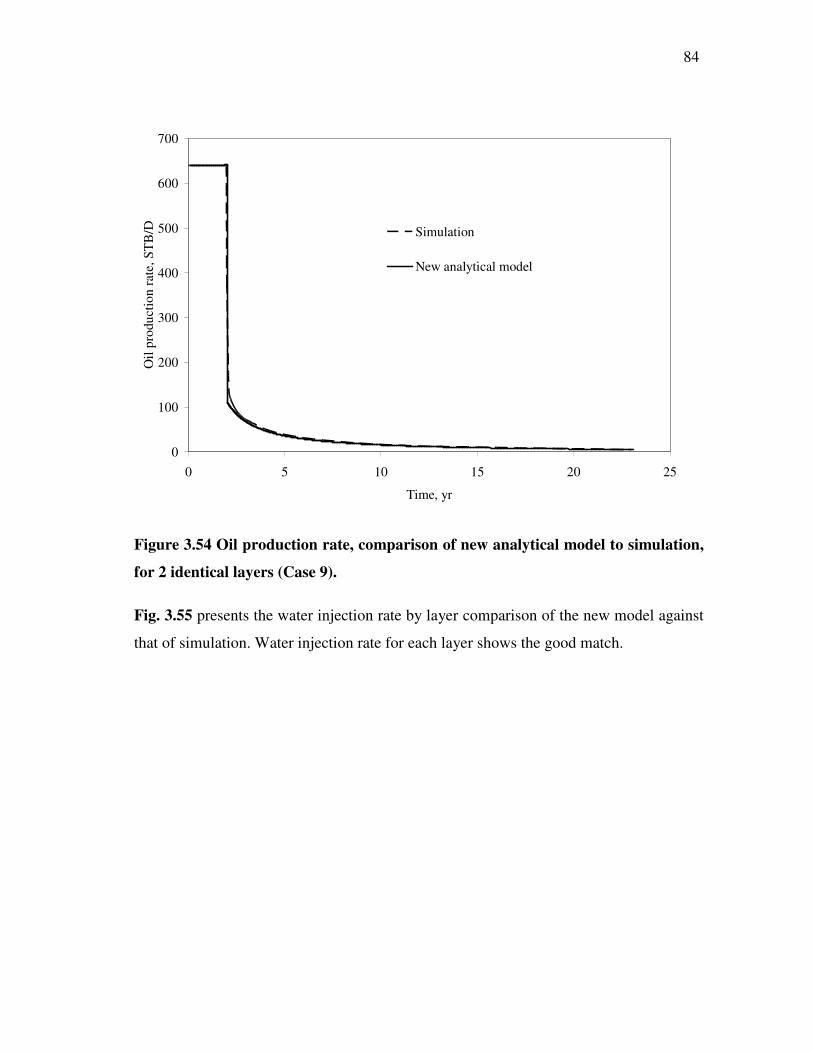
84 -
0
100
200
300
400
500
600
700
0 5 10 15 20 25
Time, yr
Oil
prod
uctio
n ra
te, S
TB
/D Simulation
New analytical model
Figure 3.54 Oil production rate, comparison of new analytical model to simulation,
for 2 identical layers (Case 9).
Fig. 3.55 presents the water injection rate by layer comparison of the new model against
that of simulation. Water injection rate for each layer shows the good match.

85 -
200
250
300
350
400
450
0 5 10 15 20 25
Time, yr
Inje
ctio
n ra
te, S
TB
/D
Simulation, layer 1
Simulation, layer 2
New analytical model, layer 1
New analytical model, layer 2
Figure 3.55 Water injection rate by layers, comparison of new analytical model to
simulation, for 2 identical layers (Case 9).
Fig. 3.56 presents the cumulative oil production comparison of the new model against
that of simulation, showing a very good agreement.
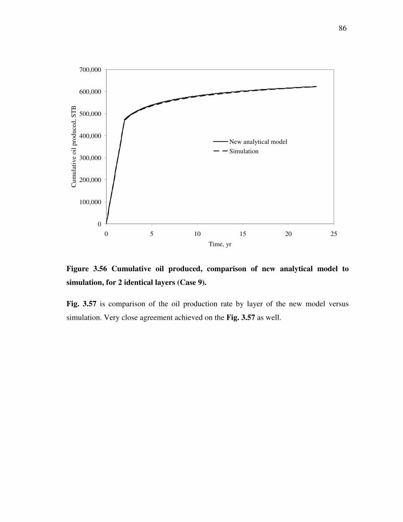
86 -
0
100,000
200,000
300,000
400,000
500,000
600,000
700,000
0 5 10 15 20 25
Time, yr
Cum
ulat
ive
oil p
rodu
ced,
ST
B
New analytical modelSimulation
Figure 3.56 Cumulative oil produced, comparison of new analytical model to
simulation, for 2 identical layers (Case 9).
Fig. 3.57 is comparison of the oil production rate by layer of the new model versus
simulation. Very close agreement achieved on the Fig. 3.57 as well.
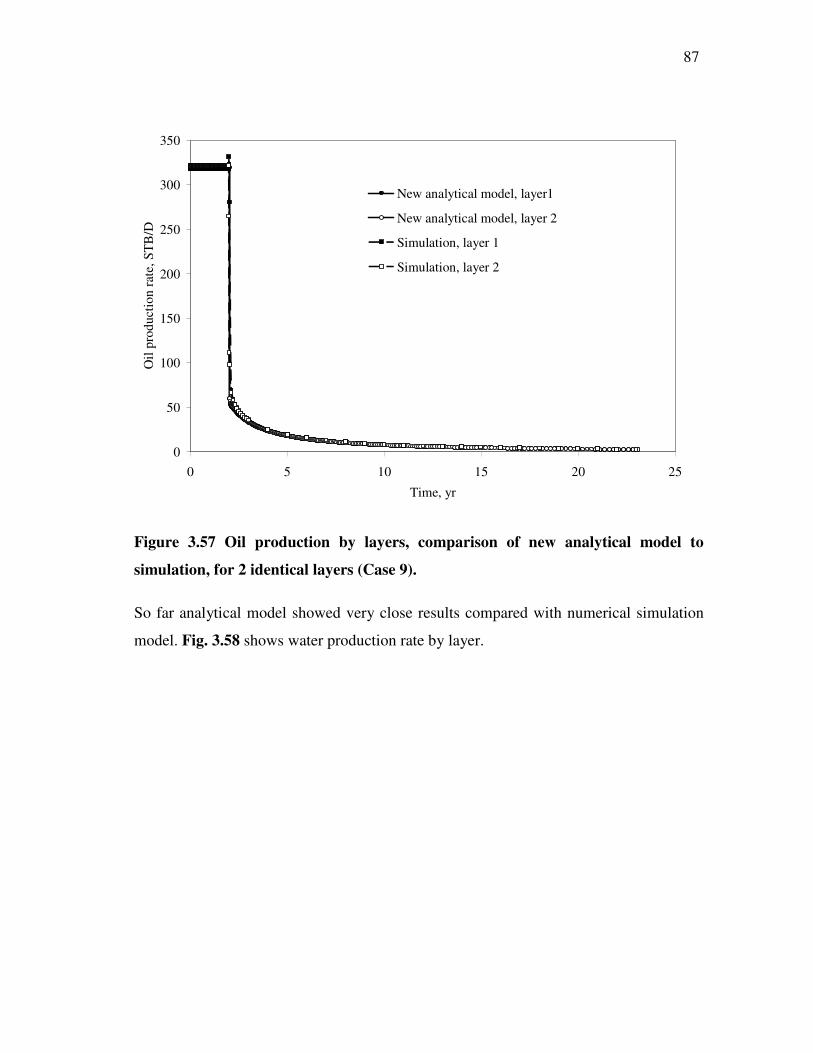
87 -
0
50
100
150
200
250
300
350
0 5 10 15 20 25
Time, yr
Oil
prod
uctio
n ra
te, S
TB
/D
New analytical model, layer1
New analytical model, layer 2
Simulation, layer 1
Simulation, layer 2
Figure 3.57 Oil production by layers, comparison of new analytical model to
simulation, for 2 identical layers (Case 9).
So far analytical model showed very close results compared with numerical simulation
model. Fig. 3.58 shows water production rate by layer.
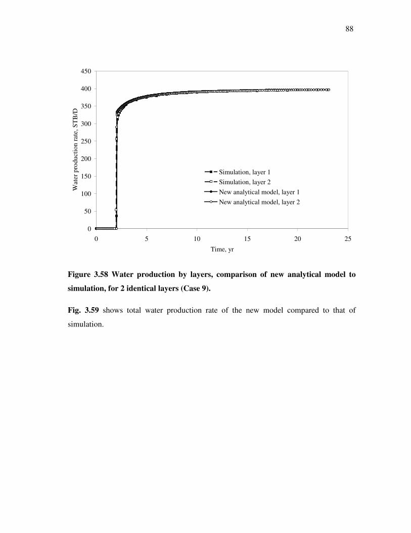
88 -
0
50
100
150
200
250
300
350
400
450
0 5 10 15 20 25
Time, yr
Wat
er p
rodu
ctio
n ra
te, S
TB
/D
Simulation, layer 1Simulation, layer 2New analytical model, layer 1New analytical model, layer 2
Figure 3.58 Water production by layers, comparison of new analytical model to
simulation, for 2 identical layers (Case 9).
Fig. 3.59 shows total water production rate of the new model compared to that of
simulation.
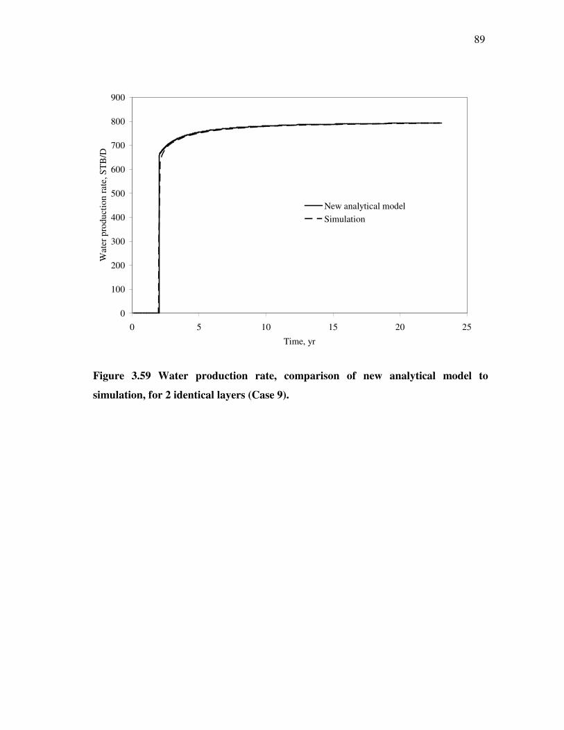
89 -
0
100
200
300
400
500
600
700
800
900
0 5 10 15 20 25
Time, yr
Wat
er p
rodu
ctio
n ra
te, S
TB
/D
New analytical modelSimulation
Figure 3.59 Water production rate, comparison of new analytical model to
simulation, for 2 identical layers (Case 9).
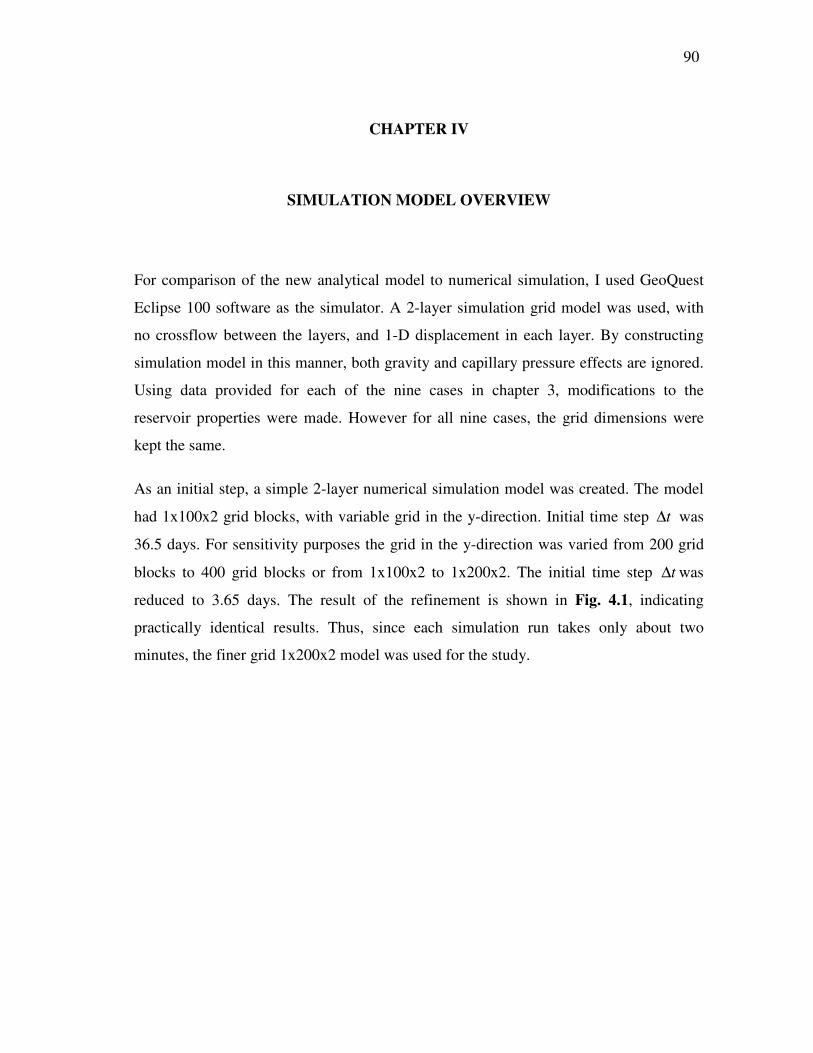
90 -
CHAPTER IV
3. SIMULATION MODEL OVERVIEW
For comparison of the new analytical model to numerical simulation, I used GeoQuest
Eclipse 100 software as the simulator. A 2-layer simulation grid model was used, with
no crossflow between the layers, and 1-D displacement in each layer. By constructing
simulation model in this manner, both gravity and capillary pressure effects are ignored.
Using data provided for each of the nine cases in chapter 3, modifications to the
reservoir properties were made. However for all nine cases, the grid dimensions were
kept the same.
As an initial step, a simple 2-layer numerical simulation model was created. The model
had 1x100x2 grid blocks, with variable grid in the y-direction. Initial time step t∆ was
36.5 days. For sensitivity purposes the grid in the y-direction was varied from 200 grid
blocks to 400 grid blocks or from 1x100x2 to 1x200x2. The initial time step t∆ was
reduced to 3.65 days. The result of the refinement is shown in Fig. 4.1, indicating
practically identical results. Thus, since each simulation run takes only about two
minutes, the finer grid 1x200x2 model was used for the study.
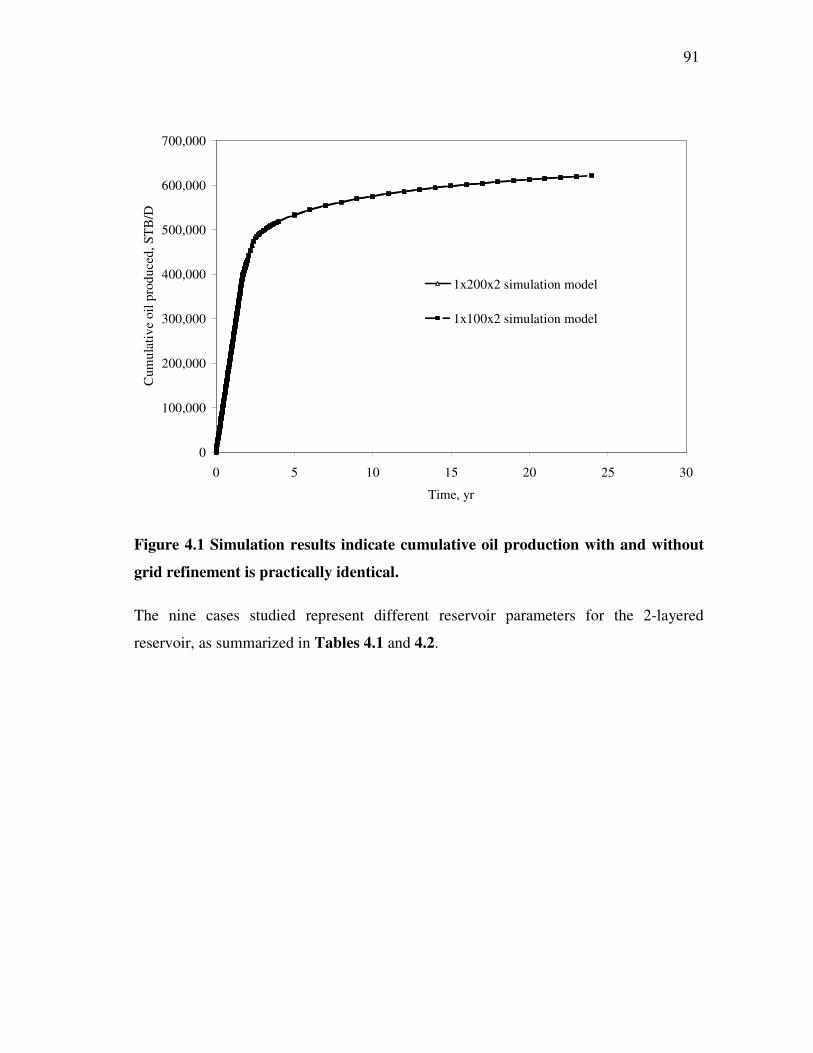
91 -
0
100,000
200,000
300,000
400,000
500,000
600,000
700,000
0 5 10 15 20 25 30
Time, yr
Cum
ulat
ive
oil p
rodu
ced,
ST
B/D
1x200x2 simulation model
1x100x2 simulation model
Figure 4.1 Simulation results indicate cumulative oil production with and without
grid refinement is practically identical.
The nine cases studied represent different reservoir parameters for the 2-layered
reservoir, as summarized in Tables 4.1 and 4.2.
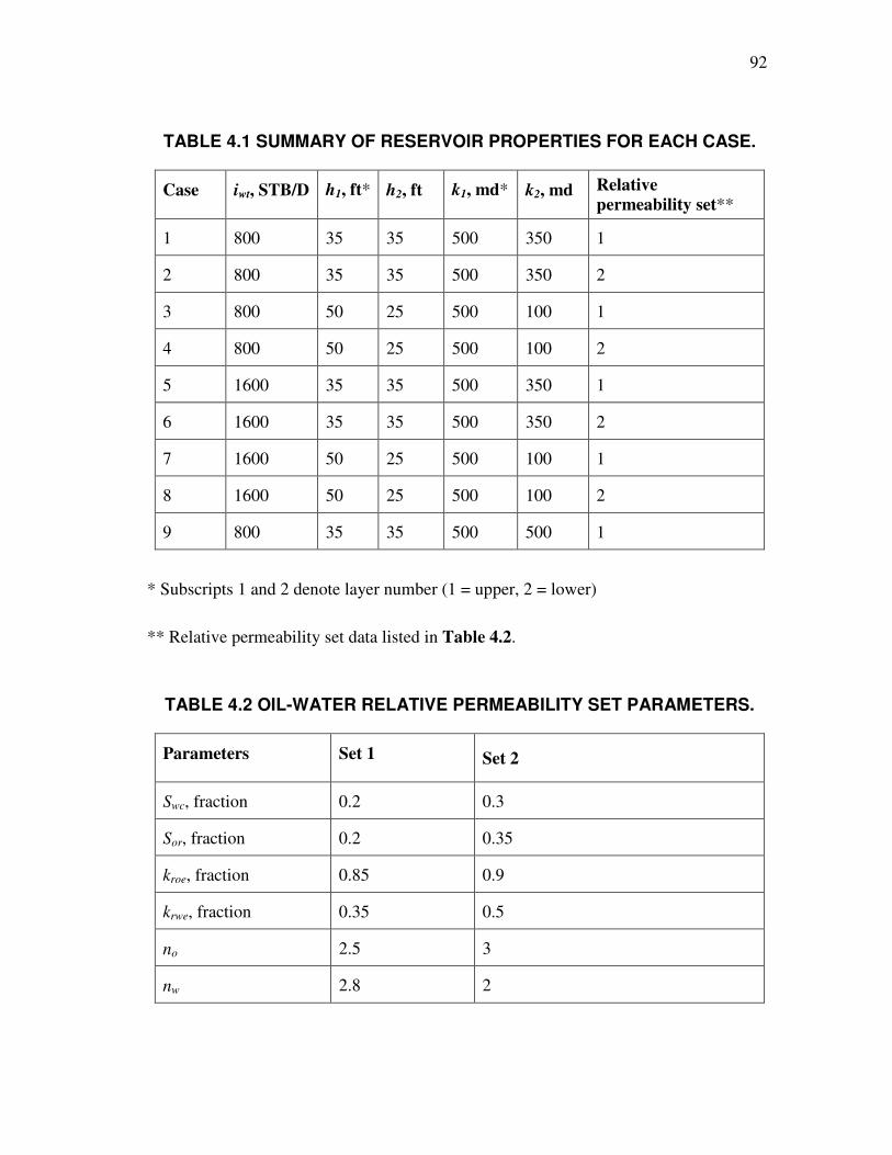
92 -
TABLE 4.1 SUMMARY OF RESERVOIR PROPERTIES FOR EACH CASE.
Case iwt, STB/D h1, ft* h2, ft k1, md* k2, md Relative permeability set**
1 800 35 35 500 350 1
2 800 35 35 500 350 2
3 800 50 25 500 100 1
4 800 50 25 500 100 2
5 1600 35 35 500 350 1
6 1600 35 35 500 350 2
7 1600 50 25 500 100 1
8 1600 50 25 500 100 2
9 800 35 35 500 500 1
* Subscripts 1 and 2 denote layer number (1 = upper, 2 = lower)
** Relative permeability set data listed in Table 4.2.
TABLE 4.2 OIL-WATER RELATIVE PERMEABILITY SET PARAMETERS.
Parameters Set 1 Set 2
Swc, fraction 0.2 0.3
Sor, fraction 0.2 0.35
kroe, fraction 0.85 0.9
krwe, fraction 0.35 0.5
no 2.5 3
nw 2.8 2

93 -
The effect of varying the parameters for each of the nine cases is significant, as shown in
Figs. 4.2 – 4.10. These figures show the oil saturation profile in each layer at 274 days
since injection, from which we can see the different waterflood advancement. The fact
that these advancements differ significantly for each case is desired to fully test the
validity of the new analytical model.
Figure 4.2 Simulation results for Case 1 at 274 days, showing earlier water
breakthrough in layer that has a higher kh.
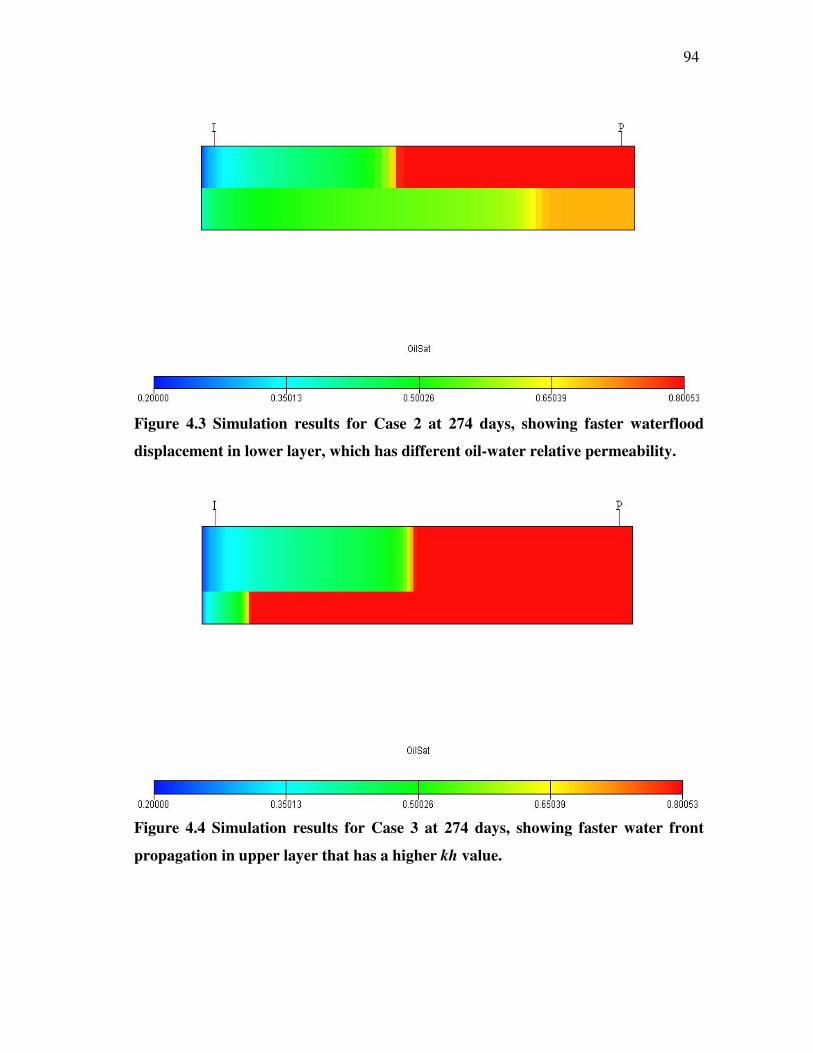
94 -
Figure 4.3 Simulation results for Case 2 at 274 days, showing faster waterflood
displacement in lower layer, which has different oil-water relative permeability.
Figure 4.4 Simulation results for Case 3 at 274 days, showing faster water front
propagation in upper layer that has a higher kh value.
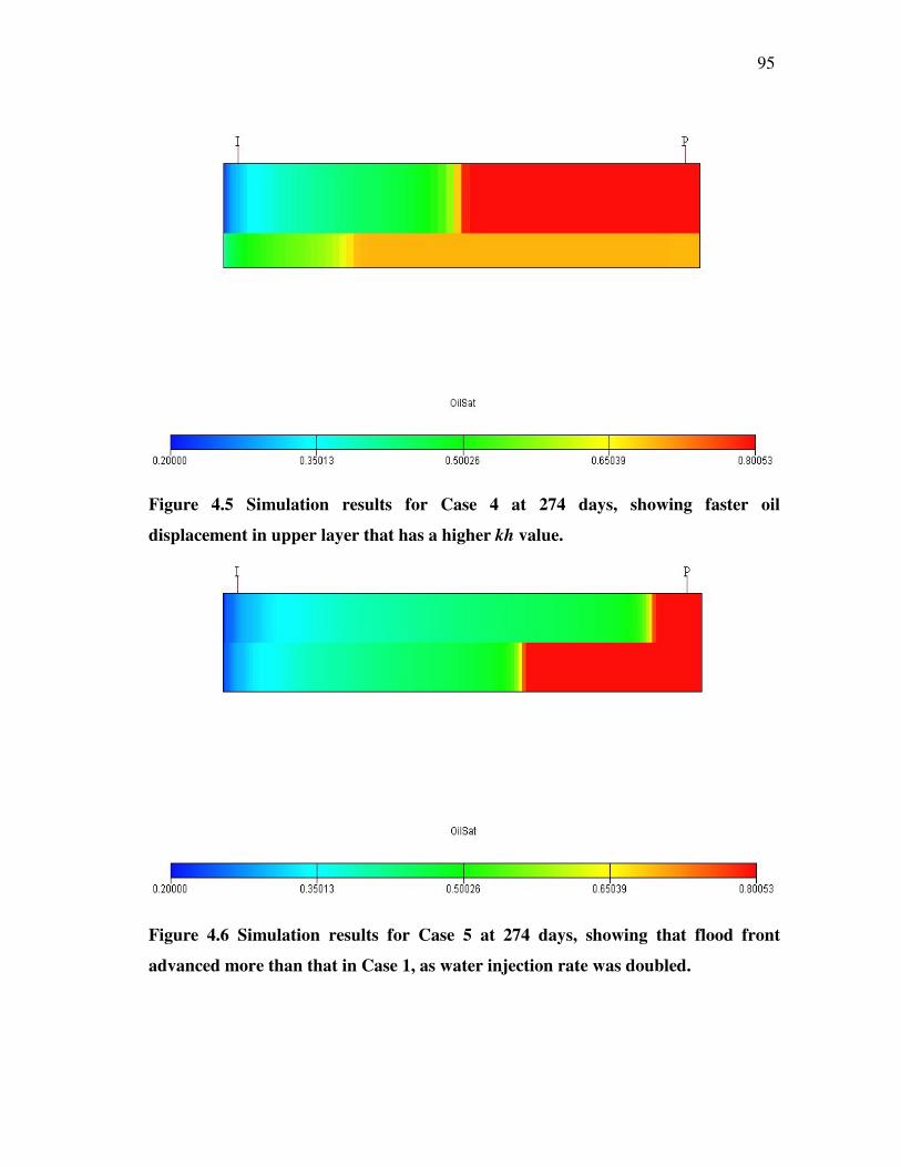
95 -
Figure 4.5 Simulation results for Case 4 at 274 days, showing faster oil
displacement in upper layer that has a higher kh value.
Figure 4.6 Simulation results for Case 5 at 274 days, showing that flood front
advanced more than that in Case 1, as water injection rate was doubled.
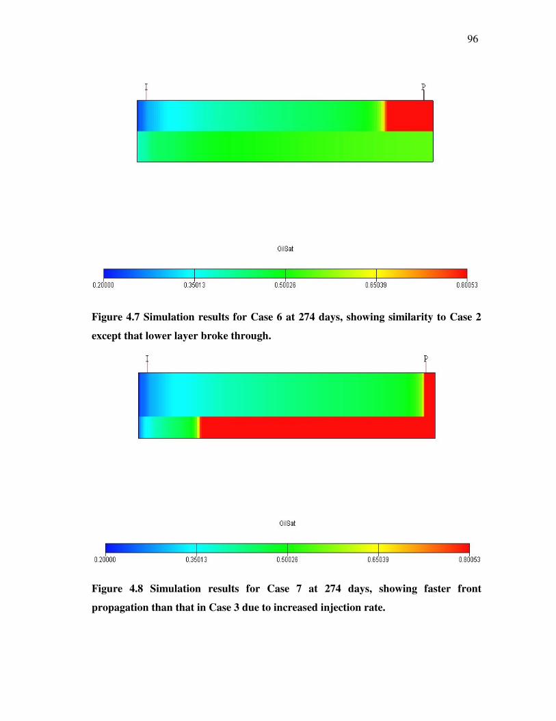
96 -
Figure 4.7 Simulation results for Case 6 at 274 days, showing similarity to Case 2
except that lower layer broke through.
Figure 4.8 Simulation results for Case 7 at 274 days, showing faster front
propagation than that in Case 3 due to increased injection rate.
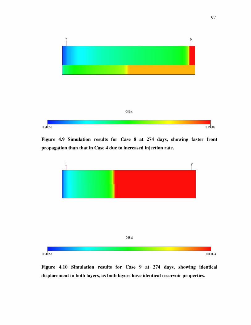
97 -
Figure 4.9 Simulation results for Case 8 at 274 days, showing faster front
propagation than that in Case 4 due to increased injection rate.
Figure 4.10 Simulation results for Case 9 at 274 days, showing identical
displacement in both layers, as both layers have identical reservoir properties.
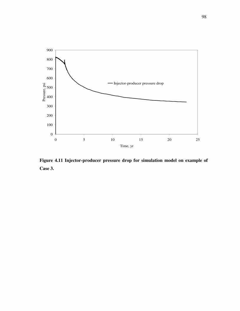
98 -
0
100
200
300
400
500
600
700
800
900
0 5 10 15 20 25
Time, yr
Pres
sure
, psi Injector-producer pressure drop
Figure 4.11 Injector-producer pressure drop for simulation model on example of
Case 3.
99 -
CHAPTER V
SUMMARY, CONCLUSIONS AND RECOMMENDATIONS
5.1 Summary
The Dykstra-Parsons model has been modified to incorporate Buckley-Leverett
displacement and the possibility of applying different oil-water relative permeability for
each layer of a multi-layered reservoir. To verify the new model, calculated results have
been compared against that of numerical simulation for a two-layered reservoir. A
computer program in Microsoft Visual Basic was written to enable solving the extensive
iterative procedure used in the new analytical method. The simulation model used was a
1x200x2 Cartesian model with no cross flow between the layers and with the constraint
of total water injection rate and total liquid production rate (in RB/D) being equal.
GeoQuest’s Eclipse 100 simulation was used in the study.
Nine cases were studied in which the following parameters were varied: total water
injection rate (800 and 1600 STB/D), layer thickness (25’, 35’, and 50’), permeability
(100, 350, and 500 md), and oil-water relative permeability (two sets of Corey type
curves).
5.2 Conclusions
Main conclusions based on the cases studied are as follows:
(1) Based on the new model, cumulative oil production (Np) up to 20 years are in good
agreement with simulation results. In the worst case studied, Np based on the new
model is 468 MSTB compared to 507 MSTB from simulation, that is a difference of
39 MSTB or 8 %.
100 -
(2) Water breakthrough times for the layer with the highest permeability-thickness
product (kh) based on the new model are in good agreement with numerical
simulation results. For the worst case studied, in which the kh product difference is
maximum between the layers and each layer has a different oil-water relative
permeability, breakthrough time based on the new model is 625 days compared to
573 days based on simulation. This is a difference of 52 days or 9 %.
(3) However, breakthrough times for the layer with the lower kh product based on the
new model are generally shorter than that based on simulation. In the worst case
studied – in which the layers have the maximum kh product contrast and the same
oil-water relative permeability set – the breakthrough time based on the new model is
1273 days compared to 2188 days based on simulation. This is an error of 915 days
or 42 %. This difference in breakthrough is due to the inaccuracy in layer injection
rate based on the new model, probably resulting from the assumption that pressure
gradient is uniform behind the front, ahead of the front and throughout a layer after
breakthrough in that layer, Nevertheless, the layer injection rate does not appear to
affect the accuracy of the total cumulative oil production after breakthrough
compared to simulation results.
(4) The initial objective of my research was to improve the vertical sweep efficiency
value in the Dykstra-Parsons model. However, a completely different approach was
subsequently developed. The main attractive capability of the new model is that it
can handle different oil-water relative permeability for each layer.
5.3 Recommendations
For future research, it is recommended to avoid the assumption of a uniform pressure
gradient behind the front, ahead of the front and throughout a layer after breakthrough in
that layer. Instead find a method to more accurately estimate pressure gradients (and thus
injector-producer pressure drop) as a function of time for each layer. By doing so, it

101 -
would be possible to arrive at a more accurate estimate of layer water injection and oil
production rates, and layer water breakthrough time.
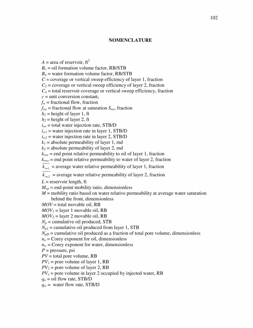
102 -
4. NOMENCLATURE
A = area of reservoir, ft2 Bo = oil formation volume factor, RB/STB Bw = water formation volume factor, RB/STB C = coverage or vertical sweep efficiency of layer 1, fraction C2 = coverage or vertical sweep efficiency of layer 2, fraction Cn = total reservoir coverage or vertical sweep efficiency, fraction c = unit conversion constant, fw = fractional flow, fraction fwe = fractional flow at saturation Swe, fraction h1 = height of layer 1, ft h2 = height of layer 2, ft iwt = total water injection rate, STB/D iw1 = water injection rate in layer 1, STB/D iw2 = water injection rate in layer 2, STB/D k1 = absolute permeability of layer 1, md k2 = absolute permeability of layer 2, md kroe = end point relative permeability to oil of layer 1, fraction krwe = end point relative permeability to water of layer 2, fraction
1rwk = average water relative permeability of layer 1, fraction
2rwk = average water relative permeability of layer 2, fraction L = reservoir length, ft Mep = end-point mobility ratio, dimensionless M = mobility ratio based on water relative permeability at average water saturation
behind the front, dimensionless MOV = total movable oil, RB MOV1 = layer 1 movable oil, RB MOV2 = layer 2 movable oil, RB Np = cumulative oil produced, STB Np1 = cumulative oil produced from layer 1, STB NpD = cumulative oil produced as a fraction of total pore volume, dimensionless no = Corey exponent for oil, dimensionless nw = Corey exponent for water, dimensionless P = pressure, psi PV = total pore volume, RB PV1 = pore volume of layer 1, RB PV2 = pore volume of layer 2, RB PVx = pore volume in layer 2 occupied by injected water, RB qo = oil flow rate, STB/D qw = water flow rate, STB/D
103 -
Swbt = water saturation at the breakthrough, fraction
wS = average water saturation behind the waterflood front, fraction Soi= initial oil saturation, fraction Swc = connate water saturation, fraction Sor = residual oil saturation t = time, days Wit = total cumulative water injected, STB Wi1 = cumulative water injected in layer 1, STB Wp = cumulative water produced, STB x1 = water distance of flood front from injector in layer 1, ft x2 = water distance of flood front from injector in layer 2 , ft µo = oil viscosity, cp µw = water viscosity, cp φ = porosity, fraction Subscripts 1 = as for layer 1 2 = as for layer 2 bt = at breakthrough D = dimensionless i = initial
104 -
5. REFERENCES
1. Leverett, M. C.: “Capillary Behavior in Porous Solids,” Trans., AIME (1941) 142,
152.
2. Buckley, S.E. and Leverett, M. C.: “Mechanism of Fluid Displacement in Sands,”
Trans., AIME, (1946) 146, 107.
3. Dykstra, H. and Parsons, R.L.: “The Prediction of Oil Recovery by Waterflooding,”
Secondary Recovery of Oil in the United States, Smith, J., Second edition, API, New
York, (1950), 160.
4. Welge, H. J.: “A Simplified Method for Computing Oil Recovery by Gas or Water
Drive,” Trans., AIME, (1952) 195, 91.
5. Dake, L.P.: Fundamentals of Reservoir Engineering, Elsevier Scientific Publishing
Co., New York City (1978) 365.
6. Stiles, W.E.: “Use of Permeability Distribution in Waterflood Calculations,” Trans.,
AIME (1949) 186, 9.
7. Johnson, J. P.: “Predicting Waterflood Performance by the Graphical Representation
of Porosity and Permeability Distribution,” JPT (November 1965) 1285.
8. Kufus, H.B., and Lynch, E.J.: “Linear Frontal Displacement in Multi-Layer Sands,”
Prod. Monthly (December, 1959) 24, No. 12, 32.
9. Hiatt, W. N.: “Injected-Fluid Coverage of Multi-Well Reservoirs with Permeability
Stratification,” Drilling and Production Practices, Johnston, K., API, San Antonio,
(1958), 165.
105 -
10. Warren, J.E., and Cosgrove, J.J.: “Prediction of Waterflood Behavior in a Stratified
System,” SPE Journal, (June, 1964), 149.
11. Reznik, A. A., Enick, R. M., Panvelker, S. B.: “An Analytical Extension of the
Dykstra-Parsons Vertical Stratification Discrete Solution to a Continuous, Real-Time
Basis,” SPE Journal, (December, 1984), 643.
12. Craig, F. F., Jr.: The Reservoir Engineering Aspects of Waterflooding, Monograph
Series, Richardson, Texas, SPE, (1993), 3.
13. Corey, A. T.: “The Interrelation between Gas and Oil Relative Permeabilities,” Prod.
Monthly, (November 1954), 19, 1, 38.
14. Craig, F. F., Jr.: Discussion of “Combination Method for Predicting Waterflood
Performance for Five-Spot Patterns in Stratified Reservoirs,” JPT (February 1964)
233.
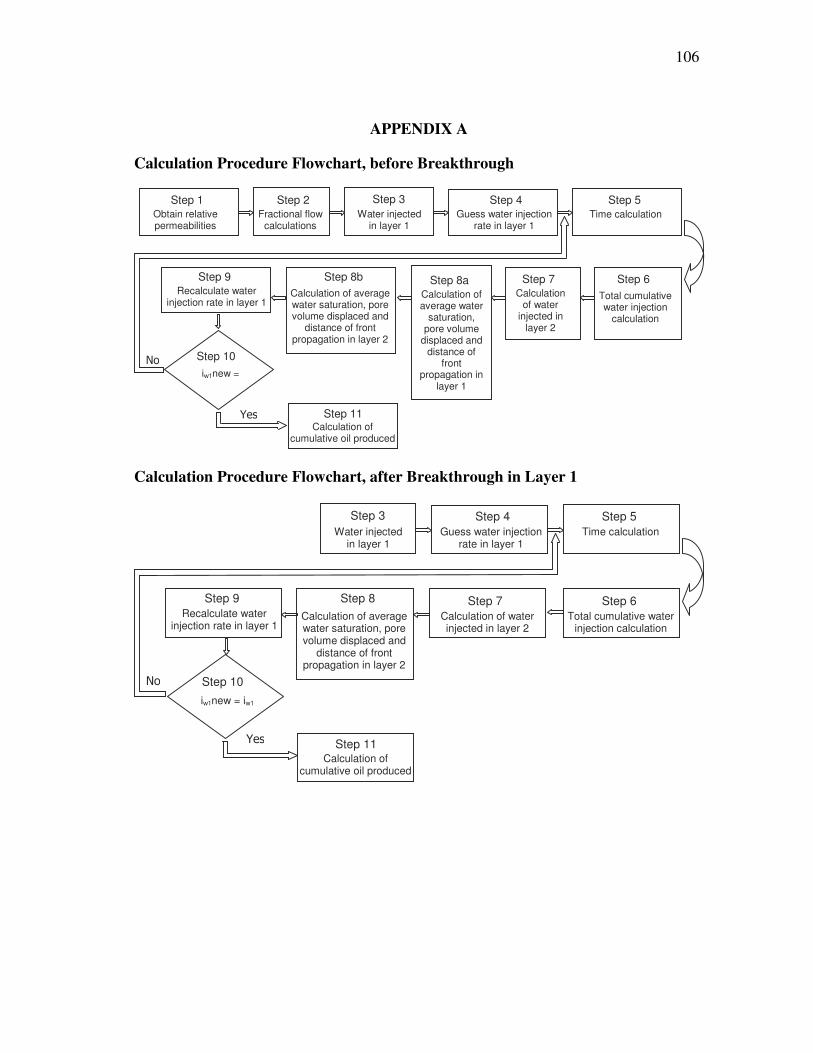
106 -
6. APPENDIX A
7. Calculation Procedure Flowchart, before Breakthrough
Calculation Procedure Flowchart, after Breakthrough in Layer 1
Step 2
Step 8b Step 7 Step 6
Step 1 Obtain relative permeabilities
Time calculation Fractional flow calculations
Water injected in layer 1
Step 3 Step 4 Guess water injection
rate in layer 1
Step 5
Total cumulative water injection
calculation
Step 9 Calculation
of water injected in
layer 2
Calculation of average water saturation, pore volume displaced and
distance of front propagation in layer 2
Recalculate water injection rate in layer 1
iw1new = i
��� Step 10
Calculation of cumulative oil produced
���� Step 11
Step 8a Calculation of average water
saturation, pore volume
displaced and distance of
front propagation in
layer 1
Step 8 Step 7 Step 6
Time calculation Water injected in layer 1
Step 3 Step 4 Guess water injection
rate in layer 1
Step 5
Total cumulative water injection calculation
Step 9 Calculation of water injected in layer 2
Calculation of average water saturation, pore volume displaced and
distance of front propagation in layer 2
Recalculate water injection rate in layer 1
iw1new = iw1
��� Step 10
Calculation of cumulative oil produced
���� Step 11
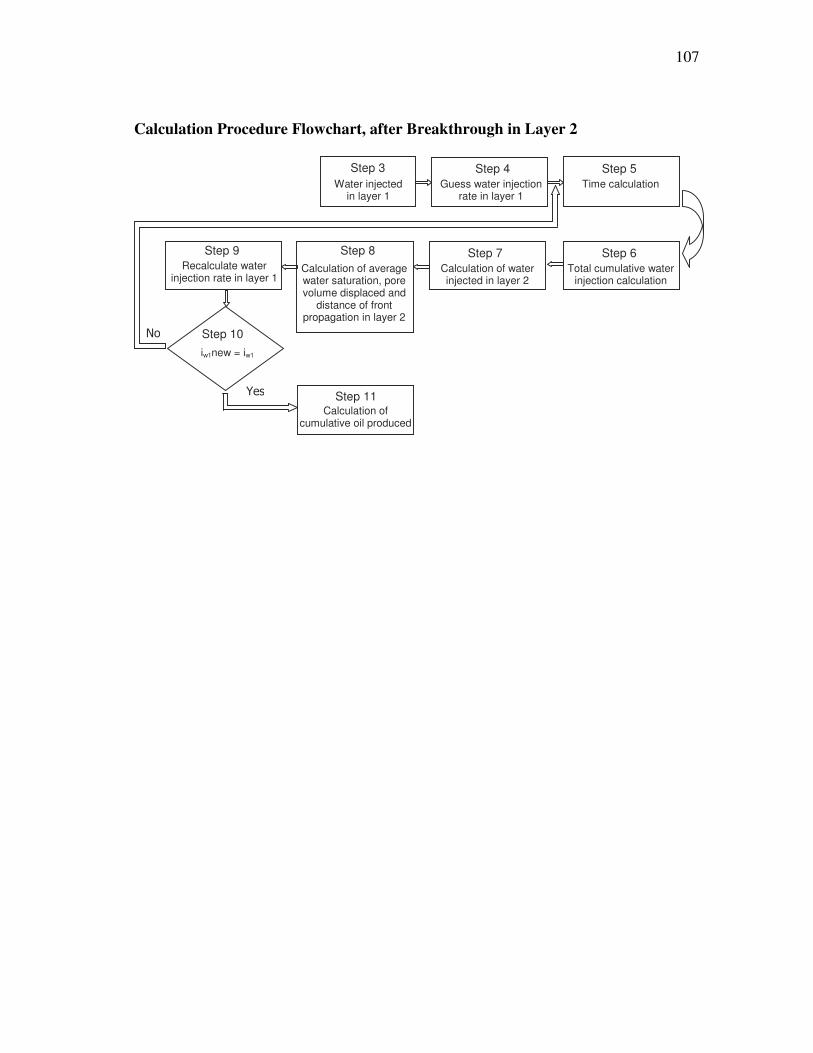
107 -
Calculation Procedure Flowchart, after Breakthrough in Layer 2
Step 8 Step 7 Step 6
Time calculation Water injected in layer 1
Step 3 Step 4 Guess water injection
rate in layer 1
Step 5
Total cumulative water injection calculation
Step 9 Calculation of water injected in layer 2
Calculation of average water saturation, pore volume displaced and
distance of front propagation in layer 2
Recalculate water injection rate in layer 1
iw1new = iw1
��� Step 10
Calculation of cumulative oil produced
���� Step 11
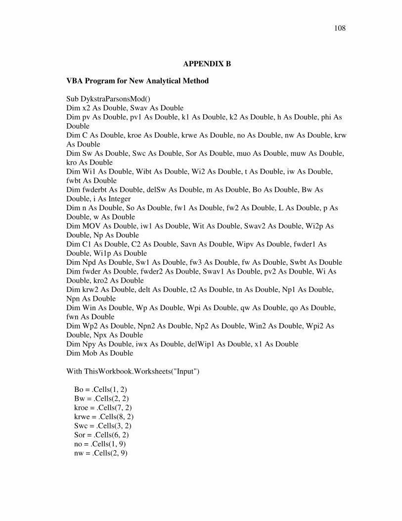
108 -
8. APPENDIX B
VBA Program for New Analytical Method Sub DykstraParsonsMod() Dim x2 As Double, Swav As Double Dim pv As Double, pv1 As Double, k1 As Double, k2 As Double, h As Double, phi As Double Dim C As Double, kroe As Double, krwe As Double, no As Double, nw As Double, krw As Double Dim Sw As Double, Swc As Double, Sor As Double, muo As Double, muw As Double, kro As Double Dim Wi1 As Double, Wibt As Double, Wi2 As Double, t As Double, iw As Double, fwbt As Double Dim fwderbt As Double, delSw As Double, m As Double, Bo As Double, Bw As Double, i As Integer Dim n As Double, So As Double, fw1 As Double, fw2 As Double, L As Double, p As Double, w As Double Dim MOV As Double, iw1 As Double, Wit As Double, Swav2 As Double, Wi2p As Double, Np As Double Dim C1 As Double, C2 As Double, Savn As Double, Wipv As Double, fwder1 As Double, Wi1p As Double Dim Npd As Double, Sw1 As Double, fw3 As Double, fw As Double, Swbt As Double Dim fwder As Double, fwder2 As Double, Swav1 As Double, pv2 As Double, Wi As Double, kro2 As Double Dim krw2 As Double, delt As Double, t2 As Double, tn As Double, Np1 As Double, Npn As Double Dim Win As Double, Wp As Double, Wpi As Double, qw As Double, qo As Double, fwn As Double Dim Wp2 As Double, Npn2 As Double, Np2 As Double, Win2 As Double, Wpi2 As Double, Npx As Double Dim Npy As Double, iwx As Double, delWip1 As Double, x1 As Double Dim Mob As Double With ThisWorkbook.Worksheets("Input") Bo = .Cells(1, 2) Bw = .Cells(2, 2) kroe = .Cells(7, 2) krwe = .Cells(8, 2) Swc = .Cells(3, 2) Sor = .Cells(6, 2) no = .Cells(1, 9) nw = .Cells(2, 9)
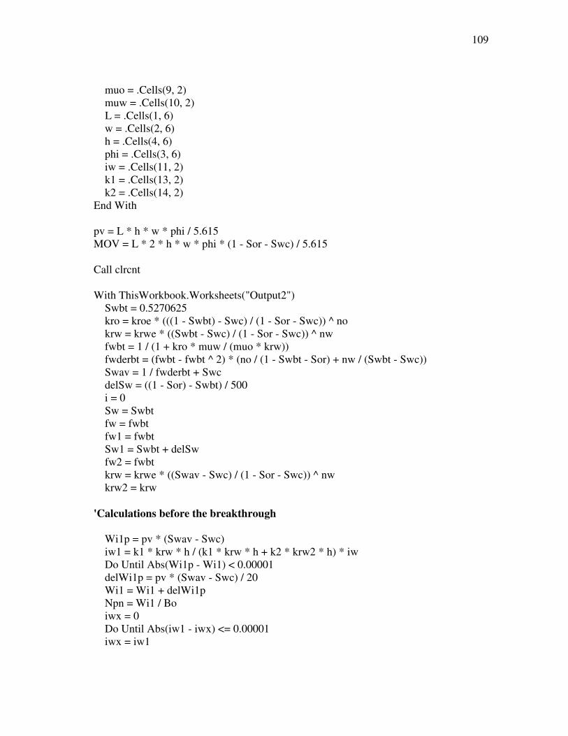
109 -
muo = .Cells(9, 2) muw = .Cells(10, 2) L = .Cells(1, 6) w = .Cells(2, 6) h = .Cells(4, 6) phi = .Cells(3, 6) iw = .Cells(11, 2) k1 = .Cells(13, 2) k2 = .Cells(14, 2) End With pv = L * h * w * phi / 5.615 MOV = L * 2 * h * w * phi * (1 - Sor - Swc) / 5.615 Call clrcnt With ThisWorkbook.Worksheets("Output2") Swbt = 0.5270625 kro = kroe * (((1 - Swbt) - Swc) / (1 - Sor - Swc)) ^ no krw = krwe * ((Swbt - Swc) / (1 - Sor - Swc)) ^ nw fwbt = 1 / (1 + kro * muw / (muo * krw)) fwderbt = (fwbt - fwbt ^ 2) * (no / (1 - Swbt - Sor) + nw / (Swbt - Swc)) Swav = 1 / fwderbt + Swc delSw = ((1 - Sor) - Swbt) / 500 i = 0 Sw = Swbt fw = fwbt fw1 = fwbt Sw1 = Swbt + delSw fw2 = fwbt krw = krwe * ((Swav - Swc) / (1 - Sor - Swc)) ^ nw krw2 = krw 'Calculations before the breakthrough Wi1p = pv * (Swav - Swc) iw1 = k1 * krw * h / (k1 * krw * h + k2 * krw2 * h) * iw Do Until Abs(Wi1p - Wi1) < 0.00001 delWi1p = pv * (Swav - Swc) / 20 Wi1 = Wi1 + delWi1p Npn = Wi1 / Bo iwx = 0 Do Until Abs(iw1 - iwx) <= 0.00001 iwx = iw1
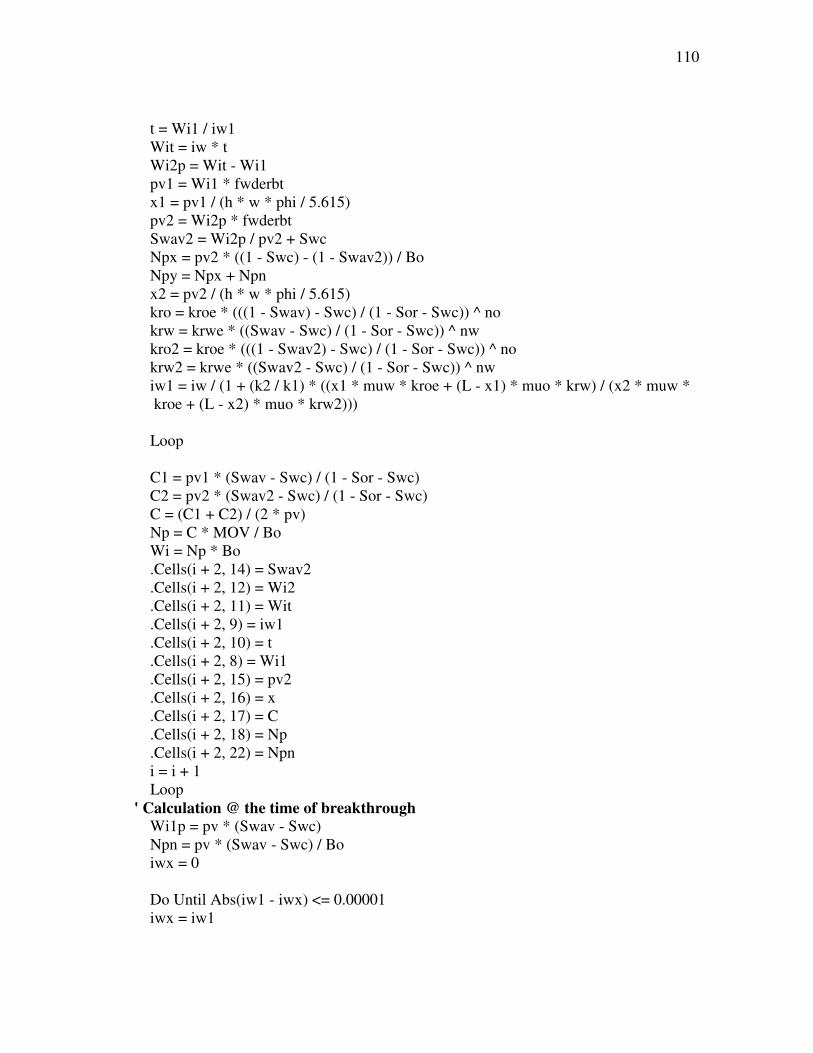
110 -
t = Wi1 / iw1 Wit = iw * t Wi2p = Wit - Wi1 pv1 = Wi1 * fwderbt x1 = pv1 / (h * w * phi / 5.615) pv2 = Wi2p * fwderbt Swav2 = Wi2p / pv2 + Swc Npx = pv2 * ((1 - Swc) - (1 - Swav2)) / Bo Npy = Npx + Npn x2 = pv2 / (h * w * phi / 5.615) kro = kroe * (((1 - Swav) - Swc) / (1 - Sor - Swc)) ^ no krw = krwe * ((Swav - Swc) / (1 - Sor - Swc)) ^ nw kro2 = kroe * (((1 - Swav2) - Swc) / (1 - Sor - Swc)) ^ no krw2 = krwe * ((Swav2 - Swc) / (1 - Sor - Swc)) ^ nw iw1 = iw / (1 + (k2 / k1) * ((x1 * muw * kroe + (L - x1) * muo * krw) / (x2 * muw *
kroe + (L - x2) * muo * krw2))) Loop C1 = pv1 * (Swav - Swc) / (1 - Sor - Swc) C2 = pv2 * (Swav2 - Swc) / (1 - Sor - Swc) C = (C1 + C2) / (2 * pv) Np = C * MOV / Bo Wi = Np * Bo .Cells(i + 2, 14) = Swav2 .Cells(i + 2, 12) = Wi2 .Cells(i + 2, 11) = Wit .Cells(i + 2, 9) = iw1 .Cells(i + 2, 10) = t .Cells(i + 2, 8) = Wi1 .Cells(i + 2, 15) = pv2 .Cells(i + 2, 16) = x .Cells(i + 2, 17) = C .Cells(i + 2, 18) = Np .Cells(i + 2, 22) = Npn i = i + 1 Loop ' Calculation @ the time of breakthrough Wi1p = pv * (Swav - Swc) Npn = pv * (Swav - Swc) / Bo iwx = 0 Do Until Abs(iw1 - iwx) <= 0.00001 iwx = iw1
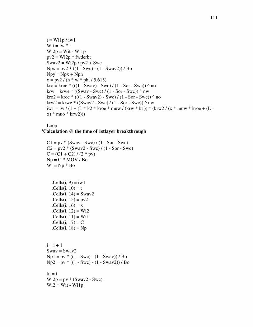
111 -
t = Wi1p / iw1 Wit = iw * t Wi2p = Wit - Wi1p pv2 = Wi2p * fwderbt Swav2 = Wi2p / pv2 + Swc Npx = pv2 * ((1 - Swc) - (1 - Swav2)) / Bo Npy = Npx + Npn x = pv2 / (h * w * phi / 5.615) kro = kroe * (((1 - Swav) - Swc) / (1 - Sor - Swc)) ^ no krw = krwe * ((Swav - Swc) / (1 - Sor - Swc)) ^ nw kro2 = kroe * (((1 - Swav2) - Swc) / (1 - Sor - Swc)) ^ no krw2 = krwe * ((Swav2 - Swc) / (1 - Sor - Swc)) ^ nw iw1 = iw / (1 + (L * k2 * kroe * muw / (krw * k1)) * (krw2 / (x * muw * kroe + (L -
x) * muo * krw2))) Loop 'Calculation @ the time of 1stlayer breakthrough C1 = pv * (Swav - Swc) / (1 - Sor - Swc) C2 = pv2 * (Swav2 - Swc) / (1 - Sor - Swc) C = (C1 + C2) / (2 * pv) Np = C * MOV / Bo Wi = Np * Bo .Cells(i, 9) = iw1 .Cells(i, 10) = t .Cells(i, 14) = Swav2 .Cells(i, 15) = pv2 .Cells(i, 16) = x .Cells(i, 12) = Wi2 .Cells(i, 11) = Wit .Cells(i, 17) = C .Cells(i, 18) = Np i = i + 1 Swav = Swav2 Np1 = pv * ((1 - Swc) - (1 - Swav)) / Bo Np2 = pv * ((1 - Swc) - (1 - Swav2)) / Bo tn = t Wi2p = pv * (Swav2 - Swc) Wi2 = Wit - Wi1p
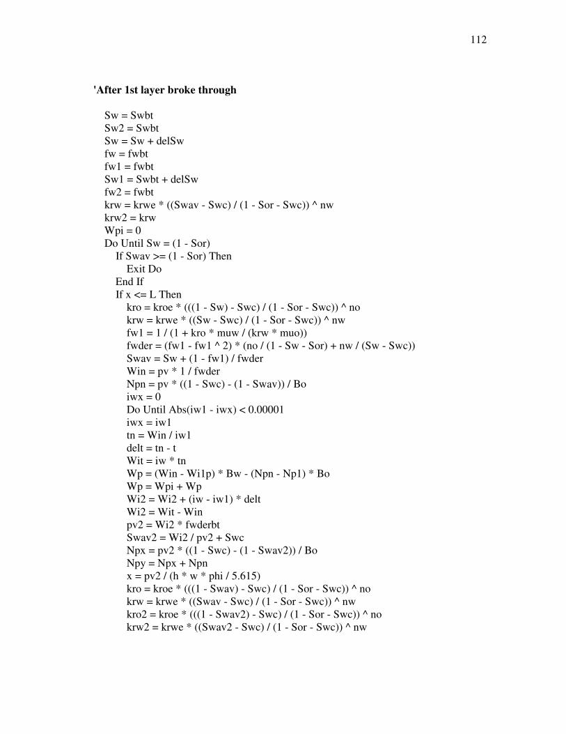
112 -
'After 1st layer broke through Sw = Swbt Sw2 = Swbt Sw = Sw + delSw fw = fwbt fw1 = fwbt Sw1 = Swbt + delSw fw2 = fwbt krw = krwe * ((Swav - Swc) / (1 - Sor - Swc)) ^ nw krw2 = krw Wpi = 0 Do Until Sw = (1 - Sor) If Swav >= (1 - Sor) Then Exit Do End If If x <= L Then kro = kroe * (((1 - Sw) - Swc) / (1 - Sor - Swc)) ^ no krw = krwe * ((Sw - Swc) / (1 - Sor - Swc)) ^ nw fw1 = 1 / (1 + kro * muw / (krw * muo)) fwder = (fw1 - fw1 ^ 2) * (no / (1 - Sw - Sor) + nw / (Sw - Swc)) Swav = Sw + (1 - fw1) / fwder Win = pv * 1 / fwder Npn = pv * ((1 - Swc) - (1 - Swav)) / Bo iwx = 0 Do Until Abs(iw1 - iwx) < 0.00001 iwx = iw1 tn = Win / iw1 delt = tn - t Wit = iw * tn Wp = (Win - Wi1p) * Bw - (Npn - Np1) * Bo Wp = Wpi + Wp Wi2 = Wi2 + (iw - iw1) * delt Wi2 = Wit - Win pv2 = Wi2 * fwderbt Swav2 = Wi2 / pv2 + Swc Npx = pv2 * ((1 - Swc) - (1 - Swav2)) / Bo Npy = Npx + Npn x = pv2 / (h * w * phi / 5.615) kro = kroe * (((1 - Swav) - Swc) / (1 - Sor - Swc)) ^ no krw = krwe * ((Swav - Swc) / (1 - Sor - Swc)) ^ nw kro2 = kroe * (((1 - Swav2) - Swc) / (1 - Sor - Swc)) ^ no krw2 = krwe * ((Swav2 - Swc) / (1 - Sor - Swc)) ^ nw
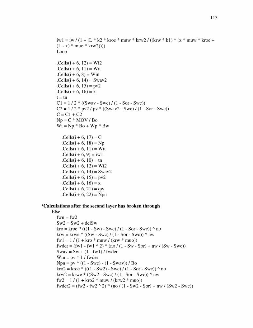
113 -
iw1 = iw / (1 + (L * k2 * kroe * muw * krw2 / ((krw * k1) * (x * muw * kroe + (L - x) * muo * krw2))))
Loop .Cells(i + 6, 12) = Wi2 .Cells(i + 6, 11) = Wit .Cells(i + 6, 8) = Win .Cells(i + 6, 14) = Swav2 .Cells(i + 6, 15) = pv2 .Cells(i + 6, 16) = x t = tn C1 = 1 / 2 * ((Swav - Swc) / (1 - Sor - Swc)) C2 = 1 / 2 * pv2 / pv * ((Swav2 - Swc) / (1 - Sor - Swc)) C = C1 + C2 Np = C * MOV / Bo Wi = Np * Bo + Wp * Bw .Cells(i + 6, 17) = C .Cells(i + 6, 18) = Np .Cells(i + 6, 11) = Wit .Cells(i + 6, 9) = iw1 .Cells(i + 6, 10) = tn .Cells(i + 6, 12) = Wi2 .Cells(i + 6, 14) = Swav2 .Cells(i + 6, 15) = pv2 .Cells(i + 6, 16) = x .Cells(i + 6, 21) = qw .Cells(i + 6, 22) = Npn ‘Calculations after the second layer has broken through Else fwn = fw2 Sw2 = Sw2 + delSw kro = kroe * (((1 - Sw) - Swc) / (1 - Sor - Swc)) ^ no krw = krwe * ((Sw - Swc) / (1 - Sor - Swc)) ^ nw fw1 = 1 / (1 + kro * muw / (krw * muo)) fwder = (fw1 - fw1 ^ 2) * (no / (1 - Sw - Sor) + nw / (Sw - Swc)) Swav = Sw + (1 - fw1) / fwder Win = pv * 1 / fwder Npn = pv * ((1 - Swc) - (1 - Swav)) / Bo kro2 = kroe * (((1 - Sw2) - Swc) / (1 - Sor - Swc)) ^ no krw2 = krwe * ((Sw2 - Swc) / (1 - Sor - Swc)) ^ nw fw2 = 1 / (1 + kro2 * muw / (krw2 * muo)) fwder2 = (fw2 - fw2 ^ 2) * (no / (1 - Sw2 - Sor) + nw / (Sw2 - Swc))
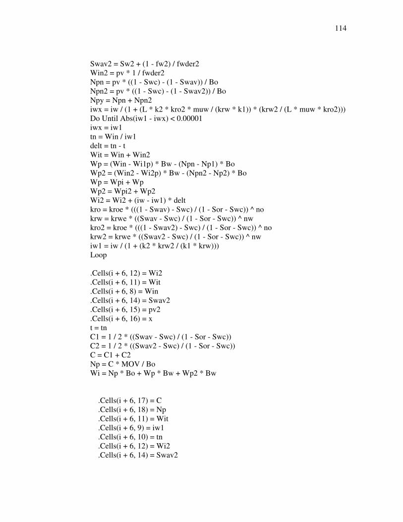
114 -
Swav2 = Sw2 + (1 - fw2) / fwder2 Win2 = pv * 1 / fwder2 Npn = pv * ((1 - Swc) - (1 - Swav)) / Bo Npn2 = pv * ((1 - Swc) - (1 - Swav2)) / Bo Npy = Npn + Npn2 iwx = iw / (1 + (L * k2 * kro2 * muw / (krw * k1)) * (krw2 / (L * muw * kro2))) Do Until Abs(iw1 - iwx) < 0.00001 iwx = iw1 tn = Win / iw1 delt = tn - t Wit = Win + Win2 Wp = (Win - Wi1p) * Bw - (Npn - Np1) * Bo Wp2 = (Win2 - Wi2p) * Bw - (Npn2 - Np2) * Bo Wp = Wpi + Wp Wp2 = Wpi2 + Wp2 Wi2 = Wi2 + (iw - iw1) * delt kro = kroe * (((1 - Swav) - Swc) / (1 - Sor - Swc)) ^ no krw = krwe * ((Swav - Swc) / (1 - Sor - Swc)) ^ nw kro2 = kroe * (((1 - Swav2) - Swc) / (1 - Sor - Swc)) ^ no krw2 = krwe * ((Swav2 - Swc) / (1 - Sor - Swc)) ^ nw iw1 = iw / (1 + (k2 * krw2 / (k1 * krw))) Loop .Cells(i + 6, 12) = Wi2 .Cells(i + 6, 11) = Wit .Cells(i + 6, 8) = Win .Cells(i + 6, 14) = Swav2 .Cells(i + 6, 15) = pv2 .Cells(i + 6, 16) = x t = tn C1 = 1 / 2 * ((Swav - Swc) / (1 - Sor - Swc)) C2 = 1 / 2 * ((Swav2 - Swc) / (1 - Sor - Swc)) C = C1 + C2 Np = C * MOV / Bo Wi = Np * Bo + Wp * Bw + Wp2 * Bw .Cells(i + 6, 17) = C .Cells(i + 6, 18) = Np .Cells(i + 6, 11) = Wit .Cells(i + 6, 9) = iw1 .Cells(i + 6, 10) = tn .Cells(i + 6, 12) = Wi2 .Cells(i + 6, 14) = Swav2

115 -
.Cells(i + 6, 15) = pv2 .Cells(i + 6, 16) = x .Cells(i + 6, 21) = qw .Cells(i + 6, 22) = Npn .Cells(i + 6, 223) = Npn2 Wpi2 = Wp2 Np2 = Npn2 Wi2p = Win2 End If Wpi = Wp i = i + 1 Np1 = Npn Wi1p = Win Sw = Sw + delSw Loop End With End Sub
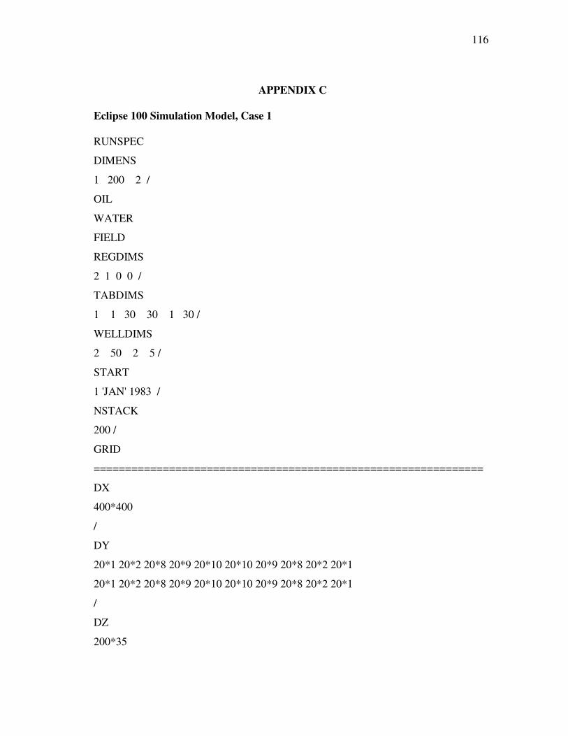
116 -
APPENDIX C Eclipse 100 Simulation Model, Case 1 RUNSPEC
DIMENS
1 200 2 /
OIL
WATER
FIELD
REGDIMS
2 1 0 0 /
TABDIMS
1 1 30 30 1 30 /
WELLDIMS
2 50 2 5 /
START
1 'JAN' 1983 /
NSTACK
200 /
GRID
==============================================================
DX
400*400
/
DY
20*1 20*2 20*8 20*9 20*10 20*10 20*9 20*8 20*2 20*1
20*1 20*2 20*8 20*9 20*10 20*10 20*9 20*8 20*2 20*1
/
DZ
200*35

117 -
200*35
/
PERMX
200*500
200*350
/
PERMY
200*500
200*350
/
PERMZ
200*50
200*35
/
BOX
1 1 1 200 1 1 /
MULTZ
200*0/
ENDBOX
TOPS
200*8000.0 /
BOX
1 1 1 200 1 1 /
PORO
200*.25
/
BOX
1 1 1 200 2 2 /
PORO
118 -
200*.25
/
ENDBOX
RPTGRID
1 1 1 1 1 0 0 0 /
GRIDFILE
2 1 /
INIT
PROPS
==============================================================
SWOF
-- Sw krw kro Pcow
0.2 0 0.85 0
0.25 0.000332936 0.683829014 0
0.3 0.0023187 0.538847423 0
0.35 0.007216059 0.414068396 0
0.4 0.016148364 0.308454264 0
0.45 0.030163141 0.220907729 0
0.5 0.050255553 0.150260191 0
0.55 0.07738113 0.095255667 0
0.6 0.112463739 0.054527525 0
0.65 0.15640102 0.0265625 0
0.7 0.210068317 0.009639196 0
0.75 0.274321643 0.001703985 0
0.8 0.35 0 0
/
PVTW
3480 1.00 3.00E-06 .9 0.0 /
PVCDO
119 -
3460 1.250 0 8 /
GRAVITY
34.2 1.07
/
ROCK
3460.0 5.0E-06 /
REGIONS
=============================================================
SATNUM
400*1 /
FIPNUM
200*1 200*2 /
SOLUTION
=============================================================
EQUIL
8087 3460 15000 0 0 0 1 0 0 /
RPTSOL
PRESSURE SWAT SGAS SOIL FIP /
RPTRST
BASIC=2 /
SUMMARY
===========================================================
RUNSUM
SEPARATE
RPTONLY
FOPR
FWPR
FWIR
FWCT
120 -
ROPR
/
RWIR
/
RWPR
/
WBHP
/
FPR
FOPT
FWPT
FWIT
FOE
FOEW
WPI
/
WPI1
/
FLPR
FLPT
FVPR
FVPT
SCHEDULE
===========================================================
RPTSCHED FIELD 16:55 18 APR 86
1 0 1 0 0 0 2 2 0 0 0 2 0 0 0 0 0
0 0 0 0 0 0 0 0 0 0 0 0 0 0 0 0 0
0 0 0 0 0 0 0 0 0 0 0 0 0 0 0 0 /
WELSPECS
121 -
'P' 'G' 1 1 8035 'OIL' /
'I' 'G' 1 200 8035 'WAT' /
/
COMPDAT
'P ' 1 1 1 2 'OPEN' 1 0 .27 3* X /
'I ' 1 200 1 2 'OPEN' 1 0 .27 3* X /
/
WCONPROD
'P' 'OPEN' 'RESV' 4* 800 /
/
WCONINJ
'I' 'WAT' 'OPEN' 'RESV' 1* 800 /
/
WECON
P 0 0 .8 /
/
TSTEP
200*3.65/
TSTEP
10*36.5/
TSTEP
10*365/
TSTEP
10*365/
END
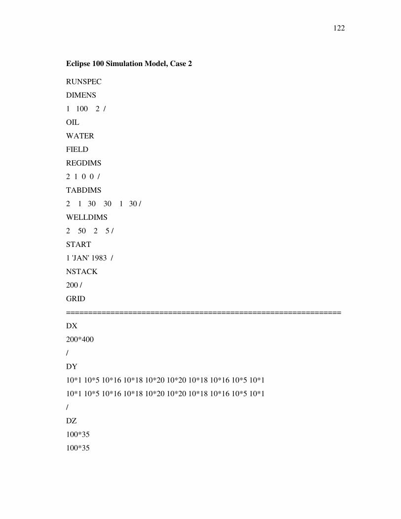
122 -
Eclipse 100 Simulation Model, Case 2 RUNSPEC
9. DIMENS
10. 1 100 2 /
11. OIL
12. WATER
13. FIELD
14. REGDIMS
15. 2 1 0 0 /
16. TABDIMS
17. 2 1 30 30 1 30 /
18. WELLDIMS
19. 2 50 2 5 /
20. START
21. 1 'JAN' 1983 /
22. NSTACK
23. 200 /
24. GRID
==============================================================
25. DX
26. 200*400
27. /
28. DY
29. 10*1 10*5 10*16 10*18 10*20 10*20 10*18 10*16 10*5 10*1
30. 10*1 10*5 10*16 10*18 10*20 10*20 10*18 10*16 10*5 10*1
31. /
32. DZ
33. 100*35
34. 100*35

123 -
35. /
36. PERMX
37. 100*500
38. 100*350
39. /
40. PERMY
41. 100*500
42. 100*350
43. /
44. PERMZ
45. 100*50
46. 100*35
47. /
48. BOX
49. 1 1 1 100 1 1 /
50. MULTZ
51. 100*0/
52. ENDBOX
53. TOPS
54. 100*8000.0 /
55. BOX
56. 1 1 1 100 1 1 /
57. PORO
58. 100*.25
59. /
60. BOX
61. 1 1 1 100 2 2 /
62. PORO
63. 100*.25
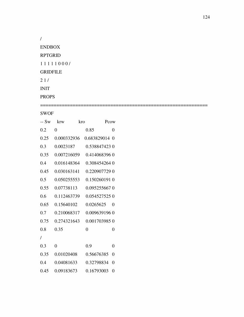
124 -
64. /
65. ENDBOX
66. RPTGRID
67. 1 1 1 1 1 0 0 0 /
68. GRIDFILE
69. 2 1 /
70. INIT
71. PROPS
==============================================================
72. SWOF
73. -- Sw krw kro Pcow
74. 0.2 0 0.85 0
75. 0.25 0.000332936 0.683829014 0
76. 0.3 0.0023187 0.538847423 0
77. 0.35 0.007216059 0.414068396 0
78. 0.4 0.016148364 0.308454264 0
79. 0.45 0.030163141 0.220907729 0
80. 0.5 0.050255553 0.150260191 0
81. 0.55 0.07738113 0.095255667 0
82. 0.6 0.112463739 0.054527525 0
83. 0.65 0.15640102 0.0265625 0
84. 0.7 0.210068317 0.009639196 0
85. 0.75 0.274321643 0.001703985 0
86. 0.8 0.35 0 0
87. /
88. 0.3 0 0.9 0
89. 0.35 0.01020408 0.56676385 0
90. 0.4 0.04081633 0.32798834 0
91. 0.45 0.09183673 0.16793003 0
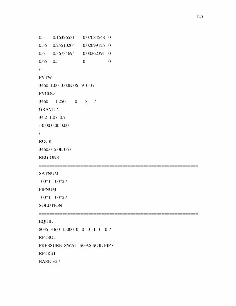
125 -
92. 0.5 0.16326531 0.07084548 0
93. 0.55 0.25510204 0.02099125 0
94. 0.6 0.36734694 0.00262391 0
95. 0.65 0.5 0 0
96. /
97. PVTW
98. 3460 1.00 3.00E-06 .9 0.0 /
99. PVCDO
100. 3460 1.250 0 8 /
101. GRAVITY
102. 34.2 1.07 0.7
103. --0.00 0.00 0.00
104. /
105. ROCK
106. 3460.0 5.0E-06 /
107. REGIONS
=============================================================
108. SATNUM
109. 100*1 100*2 /
110. FIPNUM
111. 100*1 100*2 /
112. SOLUTION
=============================================================
113. EQUIL
114. 8035 3460 15000 0 0 0 1 0 0 /
115. RPTSOL
116. PRESSURE SWAT SGAS SOIL FIP /
117. RPTRST
118. BASIC=2 /

126 -
119. SUMMARY
===========================================================
120. RUNSUM
121. SEPARATE
122. RPTONLY
123. FOPR
124. FWPR
125. FWIR
126. FWCT
127. ROPR
128. /
129. RWIR
130. /
131. RWPR
132. /
133. WBHP
134. /
135. FPR
136. FOPT
137. FWPT
138. FWIT
139. FOE
140. FOEW
141. WPI
142. /
143. WPI1
144. /
145. FLPR
146. FLPT

127 -
147. FVPR
148. FVPT
149. SCHEDULE
===========================================================
150. RPTSCHED FIELD 16:55 18 APR 86
151. 1 0 1 0 0 0 2 2 0 0 0 2 0 0 0 0 0
152. 0 0 0 0 0 0 0 0 0 0 0 0 0 0 0 0 0
153. 0 0 0 0 0 0 0 0 0 0 0 0 0 0 0 0 /
154. WELSPECS
155. 'P' 'G' 1 1 8035 'OIL' /
156. 'I' 'G' 1 100 8035 'WAT' /
157. /
158. COMPDAT
159. 'P ' 1 1 1 2 'OPEN' 1 0 .27 3* X /
160. 'I ' 1 100 1 2 'OPEN' 1 0 .27 3* X /
161. /
162. WCONPROD
163. 'P' 'OPEN' 'RESV' 4* 800 /
164. /
165. WCONINJ
166. 'I' 'WAT' 'OPEN' 'RESV' 1* 800 /
167. /
168. WECON
169. P 0 0 .8 /
170. /
171. TSTEP
172. 200*3.65
173. /
174. TSTEP
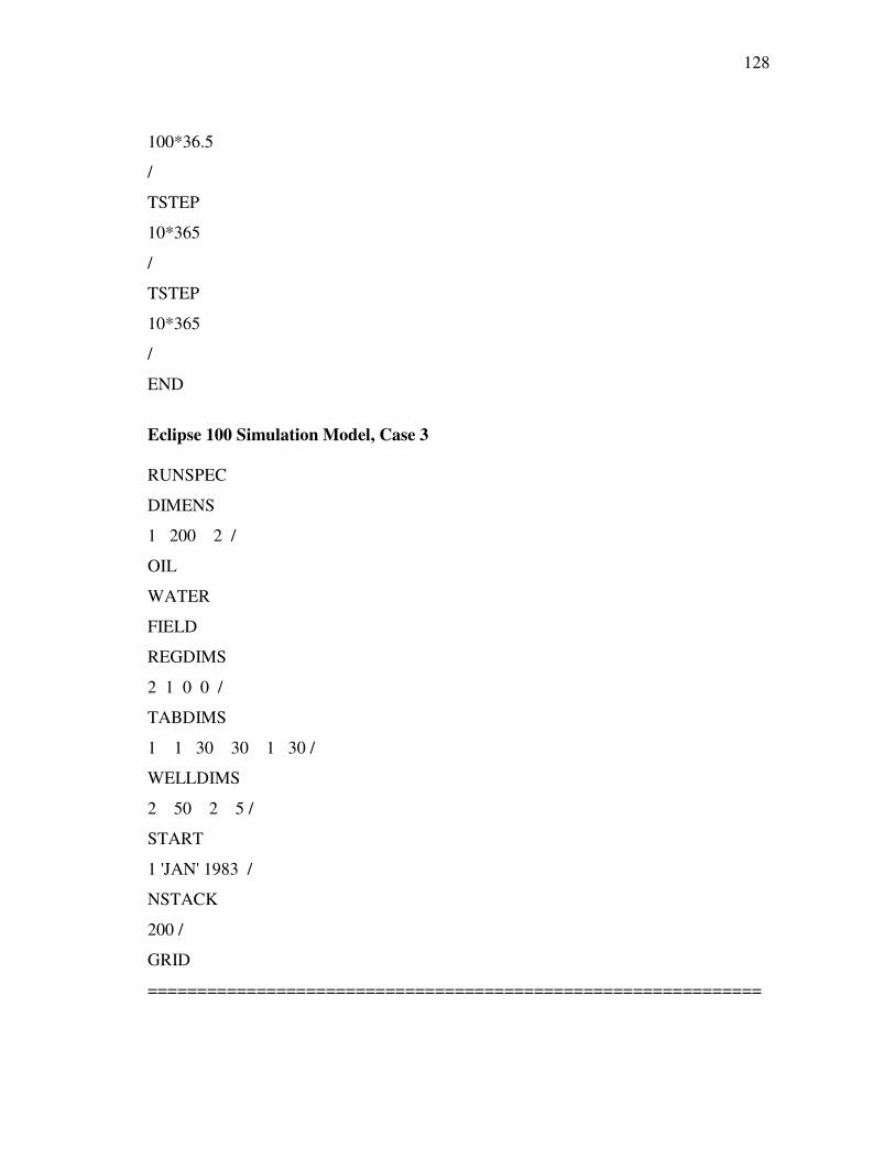
128 -
175. 100*36.5
176. /
177. TSTEP
178. 10*365
179. /
180. TSTEP
181. 10*365
182. /
END
Eclipse 100 Simulation Model, Case 3 RUNSPEC
DIMENS
1 200 2 /
OIL
WATER
FIELD
REGDIMS
2 1 0 0 /
TABDIMS
1 1 30 30 1 30 /
WELLDIMS
2 50 2 5 /
START
1 'JAN' 1983 /
NSTACK
200 /
GRID
==============================================================
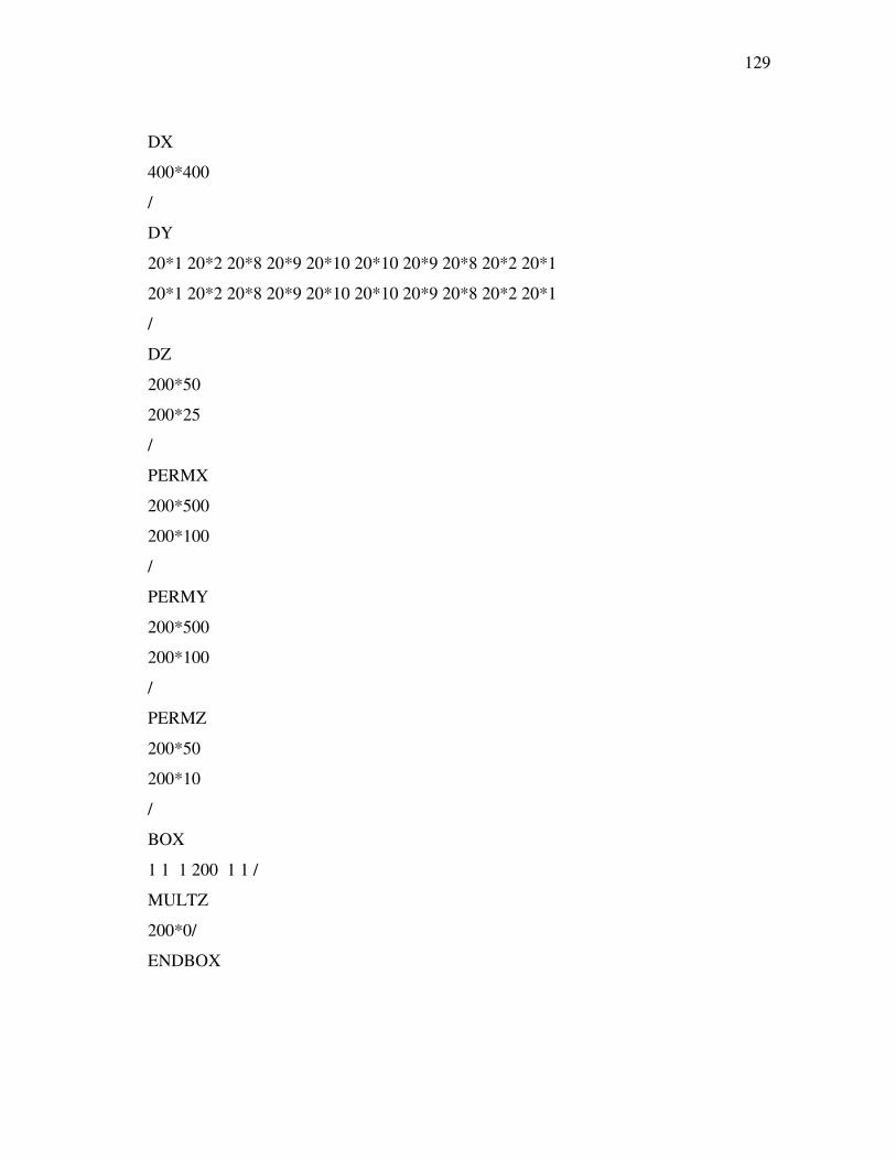
129 -
DX
400*400
/
DY
20*1 20*2 20*8 20*9 20*10 20*10 20*9 20*8 20*2 20*1
20*1 20*2 20*8 20*9 20*10 20*10 20*9 20*8 20*2 20*1
/
DZ
200*50
200*25
/
PERMX
200*500
200*100
/
PERMY
200*500
200*100
/
PERMZ
200*50
200*10
/
BOX
1 1 1 200 1 1 /
MULTZ
200*0/
ENDBOX
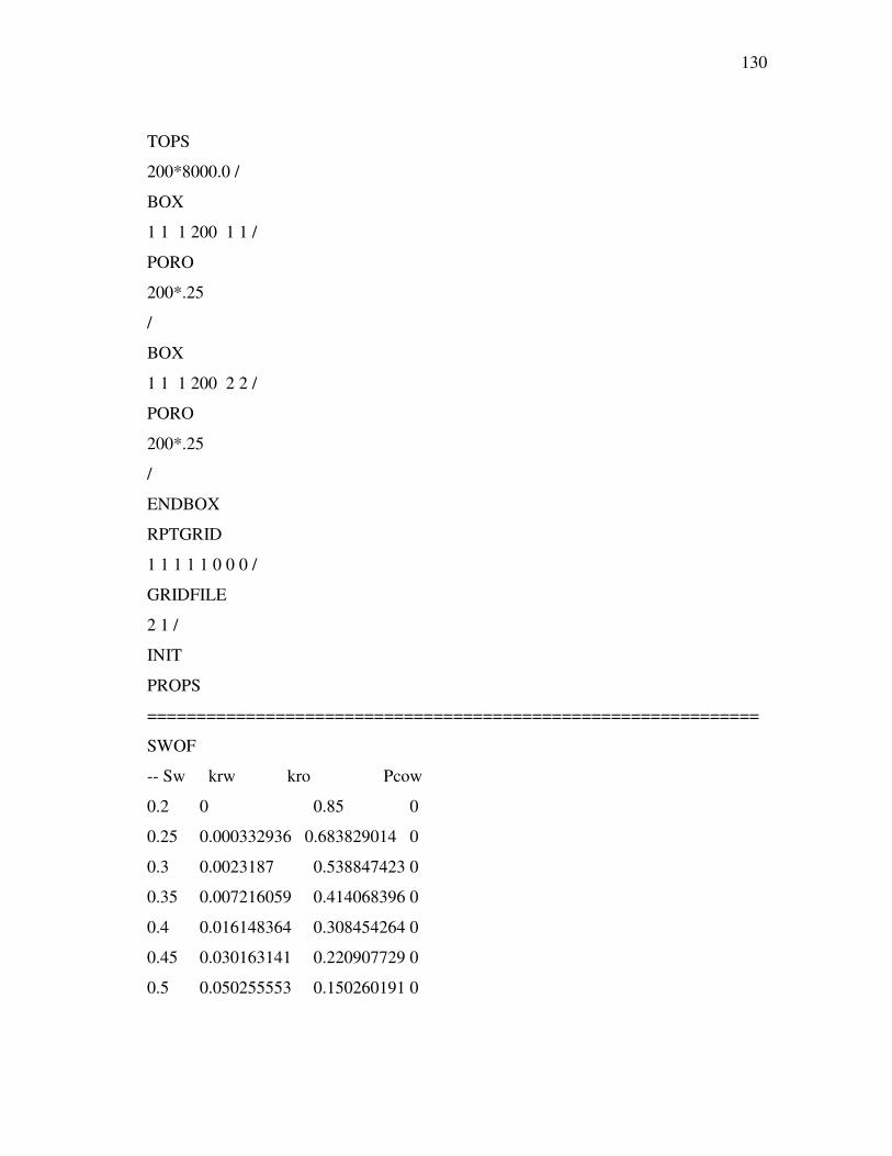
130 -
TOPS
200*8000.0 /
BOX
1 1 1 200 1 1 /
PORO
200*.25
/
BOX
1 1 1 200 2 2 /
PORO
200*.25
/
ENDBOX
RPTGRID
1 1 1 1 1 0 0 0 /
GRIDFILE
2 1 /
INIT
PROPS
==============================================================
SWOF
-- Sw krw kro Pcow
0.2 0 0.85 0
0.25 0.000332936 0.683829014 0
0.3 0.0023187 0.538847423 0
0.35 0.007216059 0.414068396 0
0.4 0.016148364 0.308454264 0
0.45 0.030163141 0.220907729 0
0.5 0.050255553 0.150260191 0
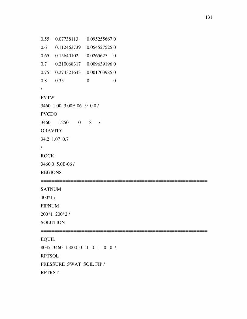
131 -
0.55 0.07738113 0.095255667 0
0.6 0.112463739 0.054527525 0
0.65 0.15640102 0.0265625 0
0.7 0.210068317 0.009639196 0
0.75 0.274321643 0.001703985 0
0.8 0.35 0 0
/
PVTW
3460 1.00 3.00E-06 .9 0.0 /
PVCDO
3460 1.250 0 8 /
GRAVITY
34.2 1.07 0.7
/
ROCK
3460.0 5.0E-06 /
REGIONS
=============================================================
SATNUM
400*1 /
FIPNUM
200*1 200*2 /
SOLUTION
=============================================================
EQUIL
8035 3460 15000 0 0 0 1 0 0 /
RPTSOL
PRESSURE SWAT SOIL FIP /
RPTRST

132 -
BASIC=2 /
SUMMARY
===========================================================
RUNSUM
SEPARATE
RPTONLY
FOPR
FWPR
FWIR
FWCT
ROPR
/
RWIR
/
RWPR
/
WBHP
/
FPR
FOPT
FWPT
FWIT
FOE
FOEW
WPI
/
WPI1
/
FLPR
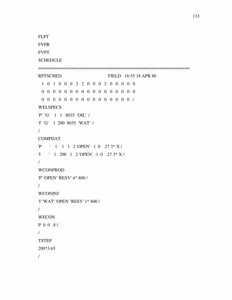
133 -
FLPT
FVPR
FVPT
SCHEDULE
===========================================================
RPTSCHED FIELD 16:55 18 APR 86
1 0 1 0 0 0 2 2 0 0 0 2 0 0 0 0 0
0 0 0 0 0 0 0 0 0 0 0 0 0 0 0 0 0
0 0 0 0 0 0 0 0 0 0 0 0 0 0 0 0 /
WELSPECS
'P' 'G' 1 1 8035 'OIL' /
'I' 'G' 1 200 8035 'WAT' /
/
COMPDAT
'P ' 1 1 1 2 'OPEN' 1 0 .27 3* X /
'I ' 1 200 1 2 'OPEN' 1 0 .27 3* X /
/
WCONPROD
'P' 'OPEN' 'RESV' 4* 800 /
/
WCONINJ
'I' 'WAT' 'OPEN' 'RESV' 1* 800 /
/
WECON
P 0 0 .8 /
/
TSTEP
200*3.65
/
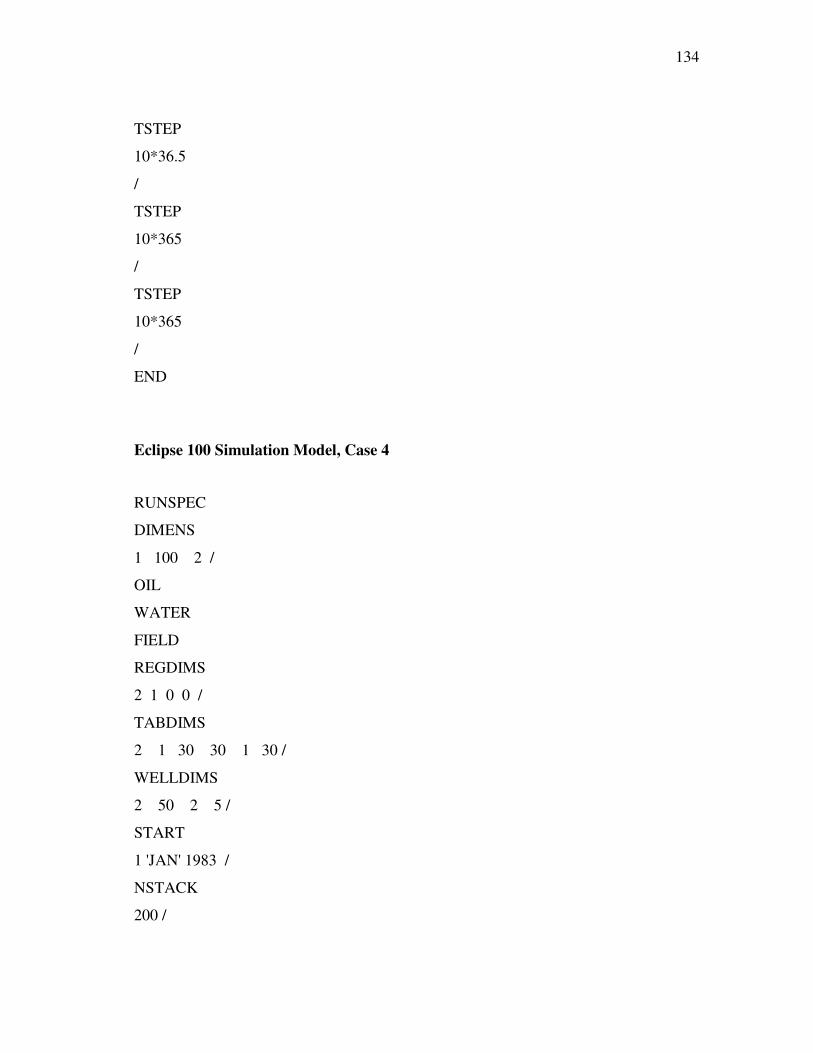
134 -
TSTEP
10*36.5
/
TSTEP
10*365
/
TSTEP
10*365
/
END
183.
Eclipse 100 Simulation Model, Case 4
184.
185. RUNSPEC
186. DIMENS
187. 1 100 2 /
188. OIL
189. WATER
190. FIELD
191. REGDIMS
192. 2 1 0 0 /
193. TABDIMS
194. 2 1 30 30 1 30 /
195. WELLDIMS
196. 2 50 2 5 /
197. START
198. 1 'JAN' 1983 /
199. NSTACK
200. 200 /
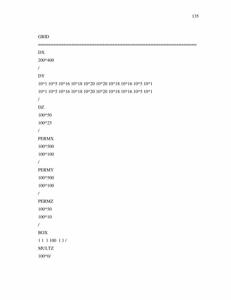
135 -
201. GRID
==============================================================
202. DX
203. 200*400
204. /
205. DY
206. 10*1 10*5 10*16 10*18 10*20 10*20 10*18 10*16 10*5 10*1
207. 10*1 10*5 10*16 10*18 10*20 10*20 10*18 10*16 10*5 10*1
208. /
209. DZ
210. 100*50
211. 100*25
212. /
213. PERMX
214. 100*500
215. 100*100
216. /
217. PERMY
218. 100*500
219. 100*100
220. /
221. PERMZ
222. 100*50
223. 100*10
224. /
225. BOX
226. 1 1 1 100 1 1 /
227. MULTZ
228. 100*0/
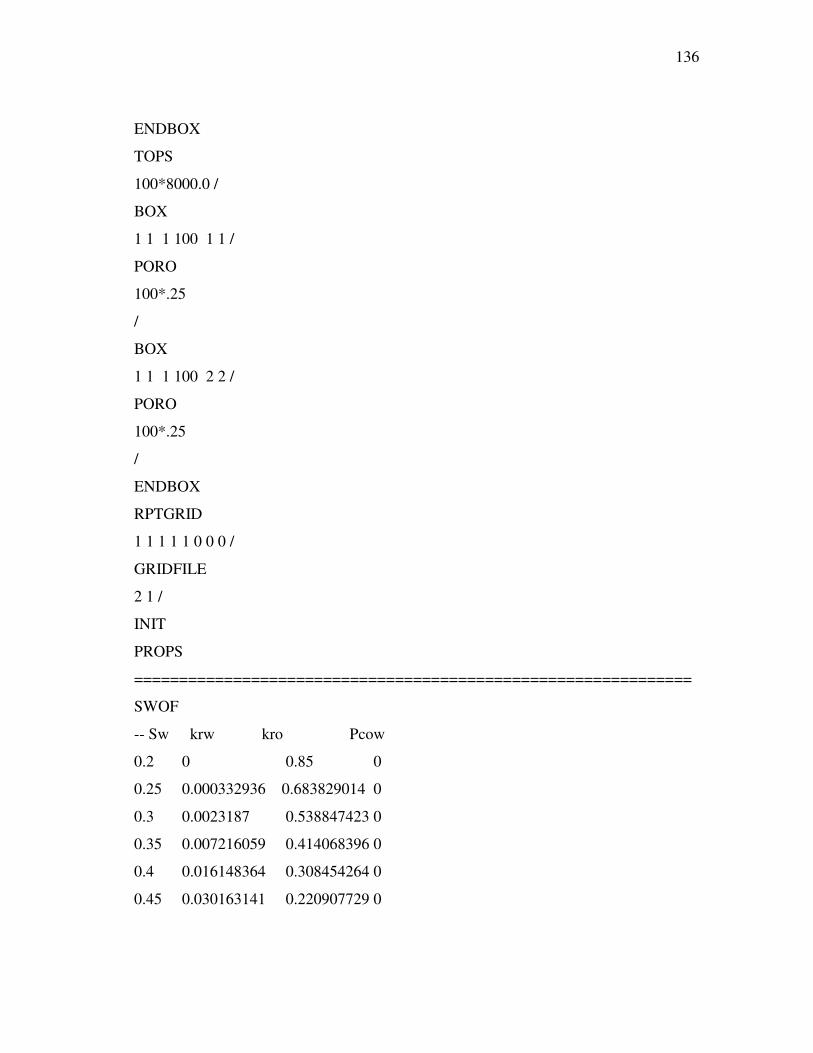
136 -
229. ENDBOX
230. TOPS
231. 100*8000.0 /
232. BOX
233. 1 1 1 100 1 1 /
234. PORO
235. 100*.25
236. /
237. BOX
238. 1 1 1 100 2 2 /
239. PORO
240. 100*.25
241. /
242. ENDBOX
243. RPTGRID
244. 1 1 1 1 1 0 0 0 /
245. GRIDFILE
246. 2 1 /
247. INIT
248. PROPS
==============================================================
249. SWOF
250. -- Sw krw kro Pcow
251. 0.2 0 0.85 0
252. 0.25 0.000332936 0.683829014 0
253. 0.3 0.0023187 0.538847423 0
254. 0.35 0.007216059 0.414068396 0
255. 0.4 0.016148364 0.308454264 0
256. 0.45 0.030163141 0.220907729 0
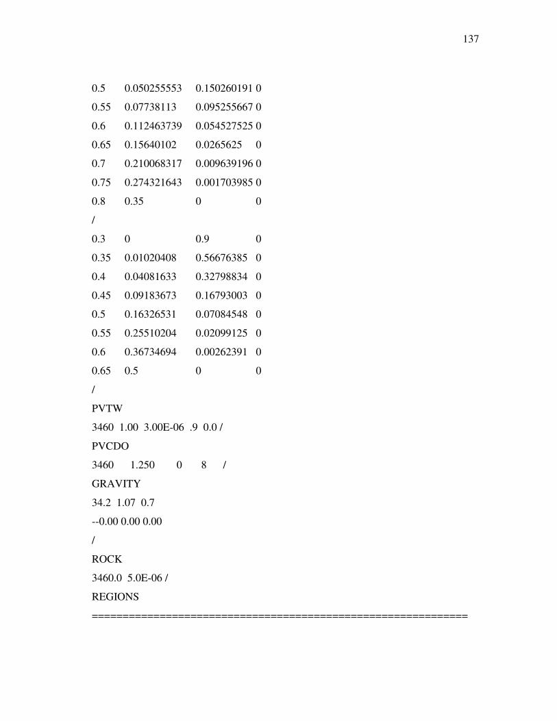
137 -
257. 0.5 0.050255553 0.150260191 0
258. 0.55 0.07738113 0.095255667 0
259. 0.6 0.112463739 0.054527525 0
260. 0.65 0.15640102 0.0265625 0
261. 0.7 0.210068317 0.009639196 0
262. 0.75 0.274321643 0.001703985 0
263. 0.8 0.35 0 0
264. /
265. 0.3 0 0.9 0
266. 0.35 0.01020408 0.56676385 0
267. 0.4 0.04081633 0.32798834 0
268. 0.45 0.09183673 0.16793003 0
269. 0.5 0.16326531 0.07084548 0
270. 0.55 0.25510204 0.02099125 0
271. 0.6 0.36734694 0.00262391 0
272. 0.65 0.5 0 0
273. /
274. PVTW
275. 3460 1.00 3.00E-06 .9 0.0 /
276. PVCDO
277. 3460 1.250 0 8 /
278. GRAVITY
279. 34.2 1.07 0.7
280. --0.00 0.00 0.00
281. /
282. ROCK
283. 3460.0 5.0E-06 /
284. REGIONS
=============================================================
138 -
285. SATNUM
286. 100*1 100*2 /
287. FIPNUM
288. 100*1 100*2 /
289. SOLUTION
=============================================================
290. EQUIL
291. 8035 3460 15000 0 0 0 1 0 0 /
292. RPTSOL
293. PRESSURE SWAT SOIL FIP /
294. RPTRST
295. BASIC=2 /
296. SUMMARY
===========================================================
297. RUNSUM
298. SEPARATE
299. RPTONLY
300. FOPR
301. FWPR
302. FWIR
303. FWCT
304. ROPR
305. /
306. RWIR
307. /
308. RWPR
309. /
310. WBHP
311. /
139 -
312. FPR
313. FOPT
314. FWPT
315. FWIT
316. FOE
317. FOEW
318. WPI
319. /
320. WPI1
321. /
322. FLPR
323. FLPT
324. FVPR
325. FVPT
326. SCHEDULE
===========================================================
327. RPTSCHED FIELD 16:55 18 APR 86
328. 1 0 1 0 0 0 2 2 0 0 0 2 0 0 0 0 0
329. 0 0 0 0 0 0 0 0 0 0 0 0 0 0 0 0 0
330. 0 0 0 0 0 0 0 0 0 0 0 0 0 0 0 0 /
331.
332. WELSPECS
333. 'P' 'G' 1 1 8035 'OIL' /
334. 'I' 'G' 1 100 8035 'WAT' /
335. /
336. COMPDAT
337. 'P ' 1 1 1 2 'OPEN' 1 0 .27 3* X /
338. 'I ' 1 100 1 2 'OPEN' 1 0 .27 3* X /
339. /
140 -
340. WCONPROD
341. 'P' 'OPEN' 'RESV' 4* 800 /
342. /
343. WCONINJ
344. 'I' 'WAT' 'OPEN' 'RESV' 1* 800 /
345. /
346. WECON
347. P 0 0 .8 /
348. /
349. TSTEP
350. 200*3.65
351. /
352. TSTEP
353. 100*36.5
354. /
355. TSTEP
356. 10*365
357. /
358. TSTEP
359. 10*365
360. /
361. END
362.
Eclipse 100 Simulation Model, Case 5
363. RUNSPEC
364. DIMENS
365. 1 200 2 /
366. OIL
141 -
367. WATER
368. FIELD
369. REGDIMS
370. 2 1 0 0 /
371. TABDIMS
372. 1 1 30 30 1 30 /
373. WELLDIMS
374. 2 50 2 5 /
375. START
376. 1 'JAN' 1983 /
377. NSTACK
378. 200 /
379. GRID
==============================================================
380. DX
381. 400*400
382. /
383. DY
384. 20*1 20*2 20*8 20*9 20*10 20*10 20*9 20*8 20*2 20*1
385. 20*1 20*2 20*8 20*9 20*10 20*10 20*9 20*8 20*2 20*1
386. /
387. DZ
388. 200*35
389. 200*35
390. /
391. PERMX
392. 200*500
393. 200*350
394. /

142 -
395. PERMY
396. 200*500
397. 200*350
398. /
PERMZ
399. 200*50
400. 200*35
401. /
402. BOX
403. 1 1 1 200 1 1 /
404. MULTZ
405. 200*0/
406. ENDBOX
407. TOPS
408. 200*8000.0 /
409. BOX
410. 1 1 1 200 1 1 /
411. PORO
412. 200*.25
413. /
414. BOX
415. 1 1 1 200 2 2 /
416. PORO
417. 200*.25
418. /
419. ENDBOX
420. RPTGRID
421. 1 1 1 1 1 0 0 0 /
422. GRIDFILE
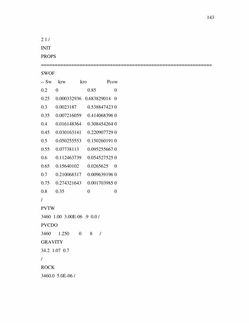
143 -
423. 2 1 /
424. INIT
425. PROPS
==============================================================
426. SWOF
427. -- Sw krw kro Pcow
428. 0.2 0 0.85 0
429. 0.25 0.000332936 0.683829014 0
430. 0.3 0.0023187 0.538847423 0
431. 0.35 0.007216059 0.414068396 0
432. 0.4 0.016148364 0.308454264 0
433. 0.45 0.030163141 0.220907729 0
434. 0.5 0.050255553 0.150260191 0
435. 0.55 0.07738113 0.095255667 0
436. 0.6 0.112463739 0.054527525 0
437. 0.65 0.15640102 0.0265625 0
438. 0.7 0.210068317 0.009639196 0
439. 0.75 0.274321643 0.001703985 0
440. 0.8 0.35 0 0
441. /
442. PVTW
443. 3460 1.00 3.00E-06 .9 0.0 /
444. PVCDO
445. 3460 1.250 0 8 /
446. GRAVITY
447. 34.2 1.07 0.7
448. /
449. ROCK
450. 3460.0 5.0E-06 /
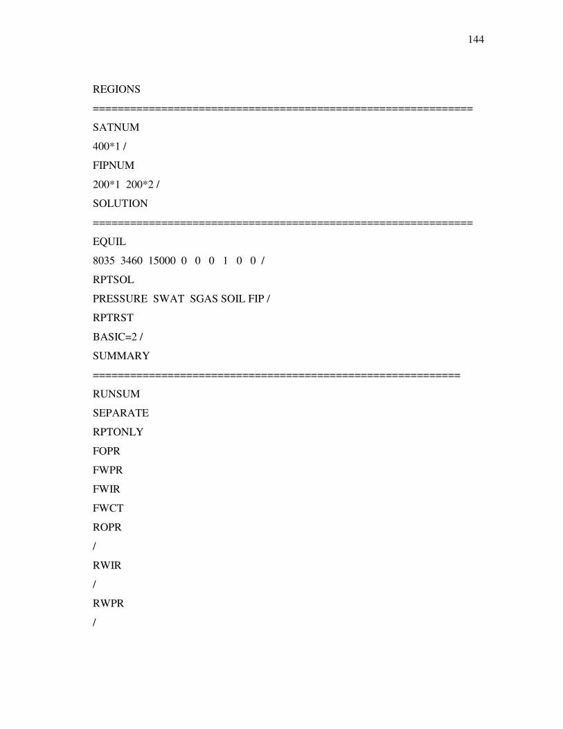
144 -
451. REGIONS
=============================================================
452. SATNUM
453. 400*1 /
454. FIPNUM
455. 200*1 200*2 /
456. SOLUTION
=============================================================
457. EQUIL
458. 8035 3460 15000 0 0 0 1 0 0 /
459. RPTSOL
460. PRESSURE SWAT SGAS SOIL FIP /
461. RPTRST
462. BASIC=2 /
463. SUMMARY
===========================================================
464. RUNSUM
465. SEPARATE
466. RPTONLY
467. FOPR
468. FWPR
469. FWIR
470. FWCT
471. ROPR
472. /
473. RWIR
474. /
475. RWPR
476. /
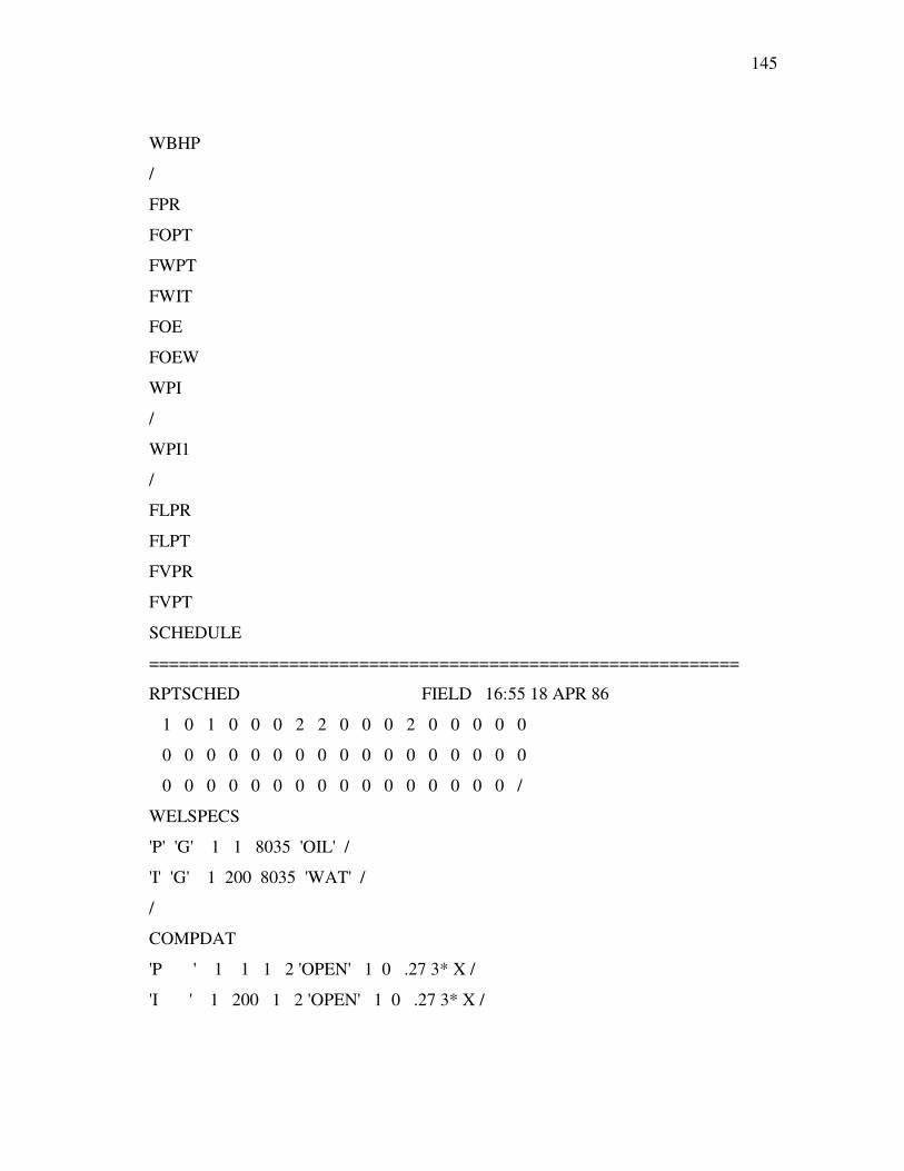
145 -
477. WBHP
478. /
479. FPR
480. FOPT
481. FWPT
482. FWIT
483. FOE
484. FOEW
485. WPI
486. /
487. WPI1
488. /
489. FLPR
490. FLPT
491. FVPR
492. FVPT
493. SCHEDULE
===========================================================
494. RPTSCHED FIELD 16:55 18 APR 86
495. 1 0 1 0 0 0 2 2 0 0 0 2 0 0 0 0 0
496. 0 0 0 0 0 0 0 0 0 0 0 0 0 0 0 0 0
497. 0 0 0 0 0 0 0 0 0 0 0 0 0 0 0 0 /
498. WELSPECS
499. 'P' 'G' 1 1 8035 'OIL' /
500. 'I' 'G' 1 200 8035 'WAT' /
501. /
502. COMPDAT
503. 'P ' 1 1 1 2 'OPEN' 1 0 .27 3* X /
504. 'I ' 1 200 1 2 'OPEN' 1 0 .27 3* X /

146 -
505. /
506. WCONPROD
507. 'P' 'OPEN' 'RESV' 4* 1600 /
508. /
509. WCONINJ
510. 'I' 'WAT' 'OPEN' 'RESV' 1* 1600 /
511. /
512. WECON
513. P 0 0 .8 /
514. /
515. TSTEP
516. 200*3.65
517. /
518. TSTEP
519. 10*36.5
520. /
521. TSTEP
522. 10*365
523. /
524. TSTEP
525. 10*365
526. /
527. END

147 -
Eclipse 100 Simulation Model, Case 6
528. RUNSPEC
529. DIMENS
530. 1 200 2 /
531. OIL
532. WATER
533. FIELD
534. REGDIMS
535. 2 1 0 0 /
536. TABDIMS
537. 2 1 30 30 1 30 /
538. WELLDIMS
539. 2 50 2 5 /
540. START
541. 1 'JAN' 1983 /
542. NSTACK
543. 200 /
544. GRID
==============================================================
545. DX
546. 400*400
547. /
548. DY
549. 20*1 20*2 20*8 20*9 20*10 20*10 20*9 20*8 20*2 20*1
550. 20*1 20*2 20*8 20*9 20*10 20*10 20*9 20*8 20*2 20*1
551. /
552. DZ
553. 200*35
554. 200*35

148 -
555. /
556. PERMX
557. 200*500
558. 200*350
559. /
560. PERMY
561. 200*500
562. 200*350
563. /
564. PERMZ
565. 200*50
566. 200*35
567. /
568. BOX
569. 1 1 1 200 1 1 /
570. MULTZ
571. 200*0/
572. ENDBOX
573. TOPS
574. 200*8000.0 /
575. BOX
576. 1 1 1 200 1 1 /
577. PORO
578. 200*.25
579. /
580. BOX
581. 1 1 1 200 2 2 /
582. PORO
583. 200*.25
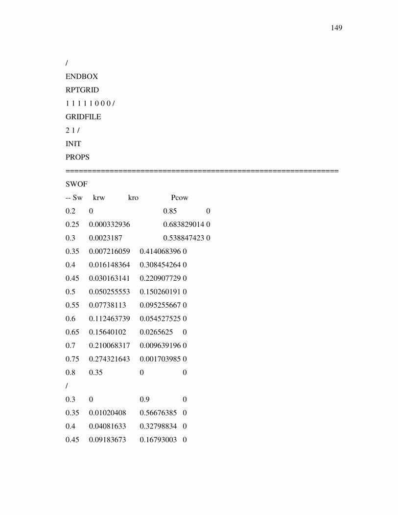
149 -
584. /
585. ENDBOX
586. RPTGRID
587. 1 1 1 1 1 0 0 0 /
588. GRIDFILE
589. 2 1 /
590. INIT
591. PROPS
==============================================================
592. SWOF
593. -- Sw krw kro Pcow
594. 0.2 0 0.85 0
595. 0.25 0.000332936 0.683829014 0
596. 0.3 0.0023187 0.538847423 0
597. 0.35 0.007216059 0.414068396 0
598. 0.4 0.016148364 0.308454264 0
599. 0.45 0.030163141 0.220907729 0
600. 0.5 0.050255553 0.150260191 0
601. 0.55 0.07738113 0.095255667 0
602. 0.6 0.112463739 0.054527525 0
603. 0.65 0.15640102 0.0265625 0
604. 0.7 0.210068317 0.009639196 0
605. 0.75 0.274321643 0.001703985 0
606. 0.8 0.35 0 0
607. /
608. 0.3 0 0.9 0
609. 0.35 0.01020408 0.56676385 0
610. 0.4 0.04081633 0.32798834 0
611. 0.45 0.09183673 0.16793003 0
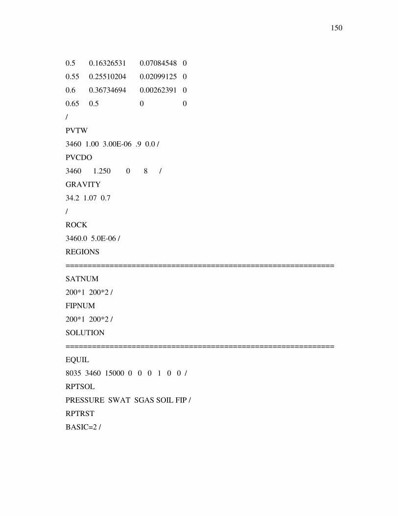
150 -
612. 0.5 0.16326531 0.07084548 0
613. 0.55 0.25510204 0.02099125 0
614. 0.6 0.36734694 0.00262391 0
615. 0.65 0.5 0 0
616. /
617. PVTW
618. 3460 1.00 3.00E-06 .9 0.0 /
619. PVCDO
620. 3460 1.250 0 8 /
621. GRAVITY
622. 34.2 1.07 0.7
623. /
624. ROCK
625. 3460.0 5.0E-06 /
626. REGIONS
=============================================================
627. SATNUM
628. 200*1 200*2 /
629. FIPNUM
630. 200*1 200*2 /
631. SOLUTION
=============================================================
632. EQUIL
633. 8035 3460 15000 0 0 0 1 0 0 /
634. RPTSOL
635. PRESSURE SWAT SGAS SOIL FIP /
636. RPTRST
637. BASIC=2 /

151 -
638. SUMMARY
===========================================================
639. RUNSUM
640. SEPARATE
641. RPTONLY
642. FOPR
643. FWPR
644. FWIR
645. FWCT
646. ROPR
647. /
648. RWIR
649. /
650. RWPR
651. /
652. WBHP
653. /
654. FPR
655. FOPT
656. FWPT
657. FWIT
658. FOE
659. FOEW
660. WPI
661. /
662. WPI1
663. /
664. FLPR
665. FLPT
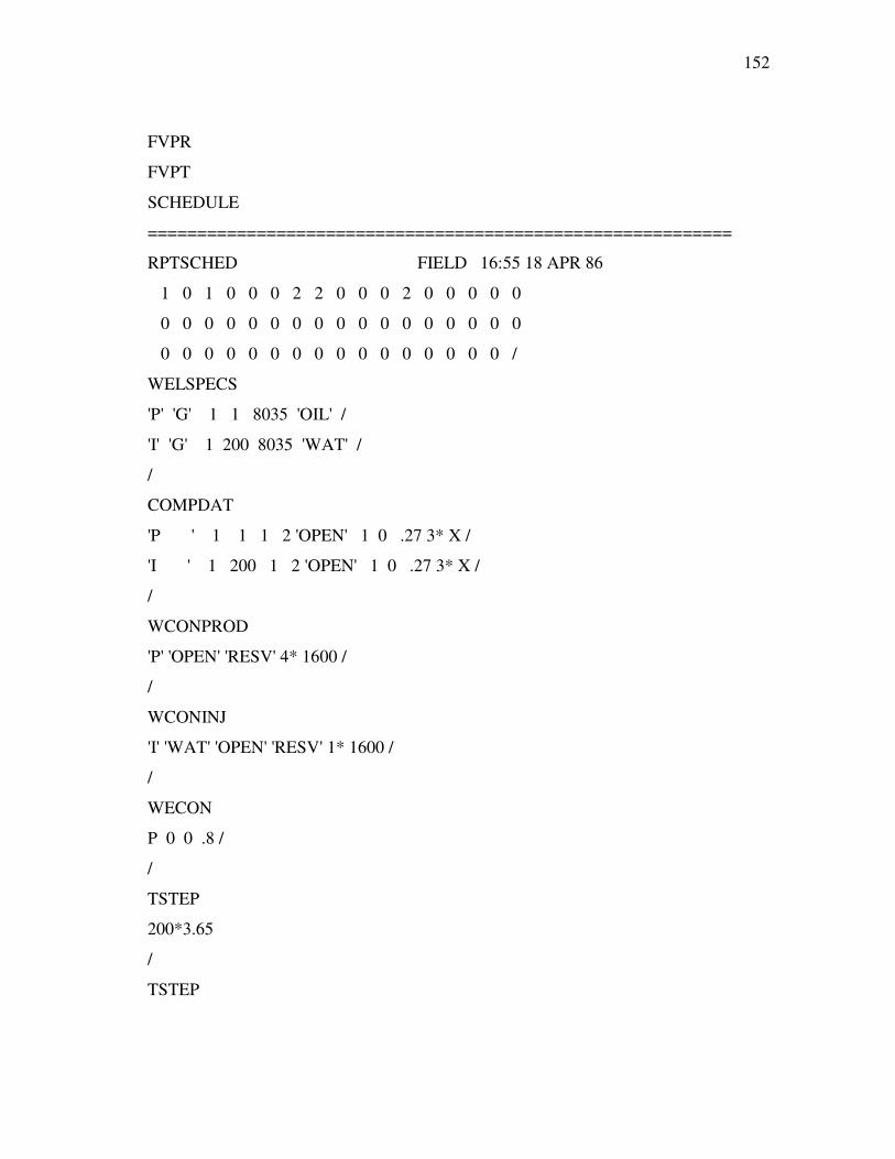
152 -
666. FVPR
667. FVPT
668. SCHEDULE
===========================================================
669. RPTSCHED FIELD 16:55 18 APR 86
670. 1 0 1 0 0 0 2 2 0 0 0 2 0 0 0 0 0
671. 0 0 0 0 0 0 0 0 0 0 0 0 0 0 0 0 0
672. 0 0 0 0 0 0 0 0 0 0 0 0 0 0 0 0 /
673. WELSPECS
674. 'P' 'G' 1 1 8035 'OIL' /
675. 'I' 'G' 1 200 8035 'WAT' /
676. /
677. COMPDAT
678. 'P ' 1 1 1 2 'OPEN' 1 0 .27 3* X /
679. 'I ' 1 200 1 2 'OPEN' 1 0 .27 3* X /
680. /
681. WCONPROD
682. 'P' 'OPEN' 'RESV' 4* 1600 /
683. /
684. WCONINJ
685. 'I' 'WAT' 'OPEN' 'RESV' 1* 1600 /
686. /
687. WECON
688. P 0 0 .8 /
689. /
690. TSTEP
691. 200*3.65
692. /
693. TSTEP
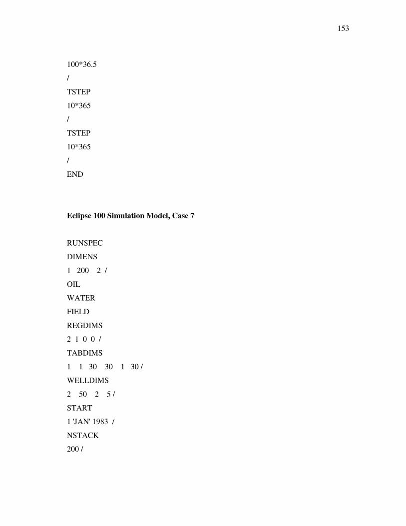
153 -
694. 100*36.5
695. /
696. TSTEP
697. 10*365
698. /
699. TSTEP
700. 10*365
701. /
702. END
703.
Eclipse 100 Simulation Model, Case 7
RUNSPEC
704. DIMENS
705. 1 200 2 /
706. OIL
707. WATER
708. FIELD
709. REGDIMS
710. 2 1 0 0 /
711. TABDIMS
712. 1 1 30 30 1 30 /
713. WELLDIMS
714. 2 50 2 5 /
715. START
716. 1 'JAN' 1983 /
717. NSTACK
718. 200 /
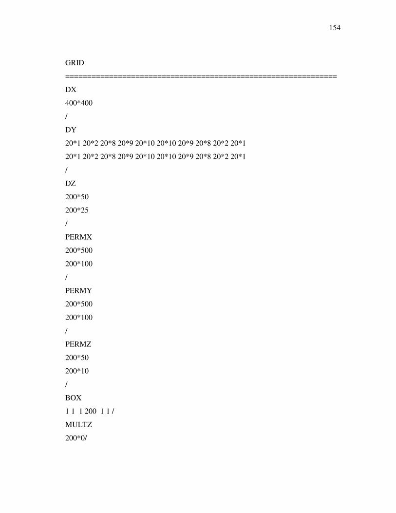
154 -
719. GRID
==============================================================
720. DX
721. 400*400
722. /
723. DY
724. 20*1 20*2 20*8 20*9 20*10 20*10 20*9 20*8 20*2 20*1
725. 20*1 20*2 20*8 20*9 20*10 20*10 20*9 20*8 20*2 20*1
726. /
727. DZ
728. 200*50
729. 200*25
730. /
731. PERMX
732. 200*500
733. 200*100
734. /
735. PERMY
736. 200*500
737. 200*100
738. /
739. PERMZ
740. 200*50
741. 200*10
742. /
743. BOX
744. 1 1 1 200 1 1 /
745. MULTZ
746. 200*0/

155 -
747. ENDBOX
748. TOPS
749. 200*8000.0 /
750. BOX
751. 1 1 1 200 1 1 /
752. PORO
753. 200*.25
754. /
755. BOX
756. 1 1 1 200 2 2 /
757. PORO
758. 200*.25
759. /
760. ENDBOX
761. RPTGRID
762. 1 1 1 1 1 0 0 0 /
763. GRIDFILE
764. 2 1 /
765. INIT
766. PROPS
==============================================================
767. SWOF
768. -- Sw krw kro Pcow
769. 0.2 0 0.85 0
770. 0.25 0.000332936 0.683829014 0
771. 0.3 0.0023187 0.538847423 0
772. 0.35 0.007216059 0.414068396 0
773. 0.4 0.016148364 0.308454264 0
774. 0.45 0.030163141 0.220907729 0
156 -
775. 0.5 0.050255553 0.150260191 0
776. 0.55 0.07738113 0.095255667 0
777. 0.6 0.112463739 0.054527525 0
778. 0.65 0.15640102 0.0265625 0
779. 0.7 0.210068317 0.009639196 0
780. 0.75 0.274321643 0.001703985 0
781. 0.8 0.35 0 0
782. /
783. PVTW
784. 3460 1.00 3.00E-06 .9 0.0 /
785. PVCDO
786. 3460 1.250 0 8 /
787. GRAVITY
788. 34.2 1.07 0.7
789. /
790. ROCK
791. 3460.0 5.0E-06 /
792. REGIONS
=============================================================
793. SATNUM
794. 400*1 /
795. FIPNUM
796. 200*1 200*2 /
797. SOLUTION
=============================================================
798. EQUIL
799. 8035 3460 15000 0 0 0 1 0 0 /
800. RPTSOL
801. PRESSURE SWAT SGAS SOIL FIP /
157 -
802. RPTRST
803. BASIC=2 /
804. SUMMARY
===========================================================
805. RUNSUM
806. SEPARATE
807. RPTONLY
808. FOPR
809. FWPR
810. FWIR
811. FWCT
812. ROPR
813. /
814. RWIR
815. /
816. RWPR
817. /
818. WBHP
819. /
820. FPR
821. FOPT
822. FWPT
823. FWIT
824. FOE
825. FOEW
826. WPI
827. /
828. WPI1
829. /
158 -
830. FLPR
831. FLPT
832. FVPR
833. FVPT
834. SCHEDULE
===========================================================
835. RPTSCHED FIELD 16:55 18 APR 86
836. 1 0 1 0 0 0 2 2 0 0 0 2 0 0 0 0 0
837. 0 0 0 0 0 0 0 0 0 0 0 0 0 0 0 0 0
838. 0 0 0 0 0 0 0 0 0 0 0 0 0 0 0 0 /
839. WELSPECS
840. 'P' 'G' 1 1 8035 'OIL' /
841. 'I' 'G' 1 200 8035 'WAT' /
842. /
843. COMPDAT
844. 'P ' 1 1 1 2 'OPEN' 1 0 .27 3* X /
845. 'I ' 1 200 1 2 'OPEN' 1 0 .27 3* X /
846. /
847. WCONPROD
848. 'P' 'OPEN' 'RESV' 4* 1600 /
849. /
850. WCONINJ
851. 'I' 'WAT' 'OPEN' 'RESV' 1* 1600 /
852. /
853. WECON
854. P 0 0 .8 /
855. /
856. TSTEP
857. 200*3.65
159 -
858. /
859. TSTEP
860. 100*3.65
861. /
862. TSTEP
863. 10*36.5
864. /
865. TSTEP
866. 10*365
867. /
868. TSTEP
869. 10*365
870. /
871. END
872.
Eclipse 100 Simulation Model, Case 8 RUNSPEC
DIMENS
1 200 2 /
OIL
WATER
FIELD
REGDIMS
2 1 0 0 /
TABDIMS
2 1 30 30 1 30 /
WELLDIMS
2 50 2 5 /

160 -
START
1 'JAN' 1983 /
NSTACK
200 /
GRID
==============================================================
DX
400*400
/
DY
20*1 20*2 20*8 20*9 20*10 20*10 20*9 20*8 20*2 20*1
20*1 20*2 20*8 20*9 20*10 20*10 20*9 20*8 20*2 20*1
/
DZ
200*50
200*25
/
PERMX
200*500
200*100
/
PERMY
200*500
200*100
/
PERMZ
200*50
200*10
/
161 -
BOX
1 1 1 200 1 1 /
MULTZ
200*0/
ENDBOX
TOPS
200*8000.0 /
BOX
1 1 1 200 1 1 /
PORO
200*.25
/
BOX
1 1 1 200 2 2 /
PORO
200*.25
/
ENDBOX
RPTGRID
1 1 1 1 1 0 0 0 /
GRIDFILE
2 1 /
INIT
PROPS
==============================================================
SWOF
-- Sw krw kro Pcow
0.2 0 0.85 0
0.25 0.000332936 0.683829014 0
162 -
0.3 0.0023187 0.538847423 0
0.35 0.007216059 0.414068396 0
0.4 0.016148364 0.308454264 0
0.45 0.030163141 0.220907729 0
0.5 0.050255553 0.150260191 0
0.55 0.07738113 0.095255667 0
0.6 0.112463739 0.054527525 0
0.65 0.15640102 0.0265625 0
0.7 0.210068317 0.009639196 0
0.75 0.274321643 0.001703985 0
0.8 0.35 0 0
/
0.3 0 0.9 0
0.35 0.01020408 0.56676385 0
0.4 0.04081633 0.32798834 0
0.45 0.09183673 0.16793003 0
0.5 0.16326531 0.07084548 0
0.55 0.25510204 0.02099125 0
0.6 0.36734694 0.00262391 0
0.65 0.5 0 0
/
PVTW
3460 1.00 3.00E-06 .9 0.0 /
PVCDO
3460 1.250 0 8 /
GRAVITY
34.2 1.07 0.7
/
163 -
ROCK
3460.0 5.0E-06 /
REGIONS
=============================================================
-- Specifies the number of saturation regions (only one for this case)
SATNUM
200*1 200*2 /
FIPNUM
200*1 200*2 /
SOLUTION
=============================================================
EQUIL
8035 3460 15000 0 0 0 1 0 0 /
RPTSOL
PRESSURE SWAT SGAS SOIL FIP /
RPTRST
BASIC=2 /
SUMMARY
===========================================================
RUNSUM
SEPARATE
RPTONLY
FOPR
FWPR
FWIR
FWCT
ROPR
/
RWIR
164 -
/
RWPR
/
WBHP
/
FPR
FOPT
FWPT
FWIT
FOE
FOEW
WPI
/
WPI1
/
FLPR
FLPT
FVPR
FVPT
SCHEDULE
===========================================================
RPTSCHED FIELD 16:55 18 APR 86
1 0 1 0 0 0 2 2 0 0 0 2 0 0 0 0 0
0 0 0 0 0 0 0 0 0 0 0 0 0 0 0 0 0
0 0 0 0 0 0 0 0 0 0 0 0 0 0 0 0 /
WELSPECS
'P' 'G' 1 1 8035 'OIL' /
'I' 'G' 1 200 8035 'WAT' /
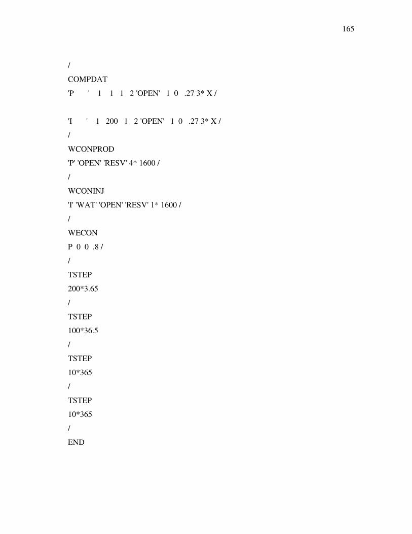
165 -
/
COMPDAT
'P ' 1 1 1 2 'OPEN' 1 0 .27 3* X /
'I ' 1 200 1 2 'OPEN' 1 0 .27 3* X /
/
WCONPROD
'P' 'OPEN' 'RESV' 4* 1600 /
/
WCONINJ
'I' 'WAT' 'OPEN' 'RESV' 1* 1600 /
/
WECON
P 0 0 .8 /
/
TSTEP
200*3.65
/
TSTEP
100*36.5
/
TSTEP
10*365
/
TSTEP
10*365
/
END
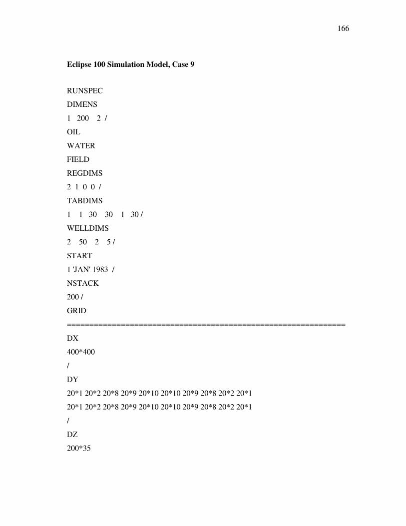
166 -
Eclipse 100 Simulation Model, Case 9 873.
874. RUNSPEC
875. DIMENS
876. 1 200 2 /
877. OIL
878. WATER
879. FIELD
880. REGDIMS
881. 2 1 0 0 /
882. TABDIMS
883. 1 1 30 30 1 30 /
884. WELLDIMS
885. 2 50 2 5 /
886. START
887. 1 'JAN' 1983 /
888. NSTACK
889. 200 /
890. GRID
==============================================================
891. DX
892. 400*400
893. /
894. DY
895. 20*1 20*2 20*8 20*9 20*10 20*10 20*9 20*8 20*2 20*1
896. 20*1 20*2 20*8 20*9 20*10 20*10 20*9 20*8 20*2 20*1
897. /
898. DZ
899. 200*35
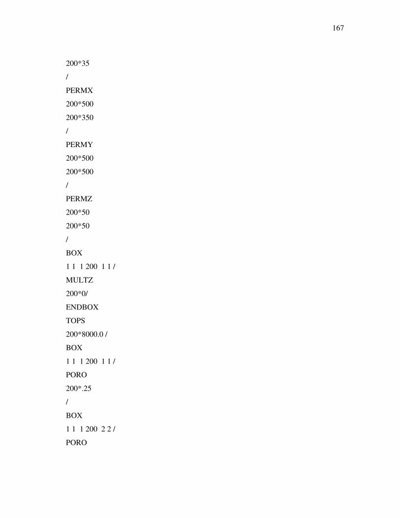
167 -
900. 200*35
901. /
902. PERMX
903. 200*500
904. 200*350
905. /
906. PERMY
907. 200*500
908. 200*500
909. /
910. PERMZ
911. 200*50
912. 200*50
913. /
914. BOX
915. 1 1 1 200 1 1 /
916. MULTZ
917. 200*0/
918. ENDBOX
919. TOPS
920. 200*8000.0 /
921. BOX
922. 1 1 1 200 1 1 /
923. PORO
924. 200*.25
925. /
926. BOX
927. 1 1 1 200 2 2 /
928. PORO
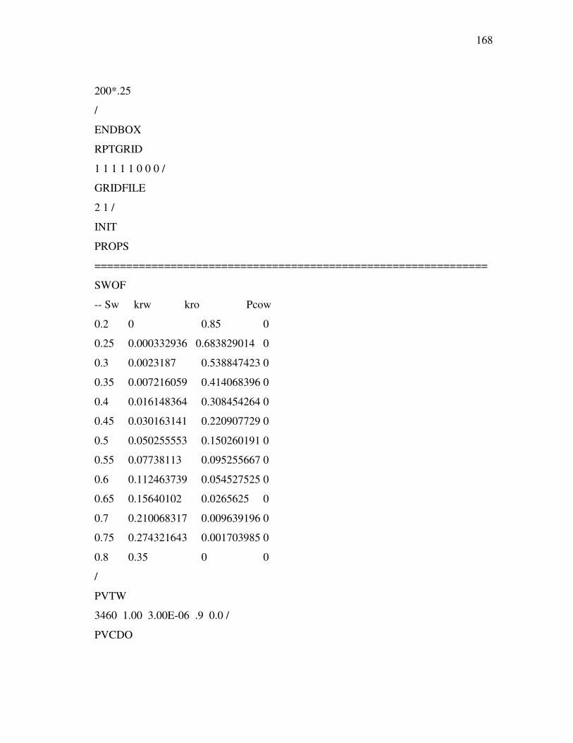
168 -
929. 200*.25
930. /
931. ENDBOX
932. RPTGRID
933. 1 1 1 1 1 0 0 0 /
934. GRIDFILE
935. 2 1 /
936. INIT
937. PROPS
==============================================================
938. SWOF
939. -- Sw krw kro Pcow
940. 0.2 0 0.85 0
941. 0.25 0.000332936 0.683829014 0
942. 0.3 0.0023187 0.538847423 0
943. 0.35 0.007216059 0.414068396 0
944. 0.4 0.016148364 0.308454264 0
945. 0.45 0.030163141 0.220907729 0
946. 0.5 0.050255553 0.150260191 0
947. 0.55 0.07738113 0.095255667 0
948. 0.6 0.112463739 0.054527525 0
949. 0.65 0.15640102 0.0265625 0
950. 0.7 0.210068317 0.009639196 0
951. 0.75 0.274321643 0.001703985 0
952. 0.8 0.35 0 0
953. /
954. PVTW
955. 3460 1.00 3.00E-06 .9 0.0 /
956. PVCDO
169 -
957. 3460 1.250 0 8 /
958. GRAVITY
959. 34.2 1.07 0.7
960. /
961. ROCK
962. 3460.0 5.0E-06 /
963. REGIONS
=============================================================
964. SATNUM
965. 400*1 /
966. FIPNUM
967. 200*1 200*2 /
968. SOLUTION
=============================================================
969. EQUIL
970. 8035 3460 15000 0 0 0 1 0 0 /
971. RPTSOL
972. PRESSURE SWAT SGAS SOIL FIP /
973. RPTRST
974. BASIC=2 /
975. SUMMARY
===========================================================
976. RUNSUM
977. SEPARATE
978. RPTONLY
979. FOPR
980. FWPR
981. FWIR
982. FWCT
170 -
983. ROPR
984. /
985. RWIR
986. /
987. RWPR
988. /
989. WBHP
990. /
991. FPR
992. FOPT
993. FWPT
994. FWIT
995. FOE
996. FOEW
997. WPI
998. /
999. WPI1
1000. /
1001. FLPR
1002. FLPT
1003. FVPR
1004. FVPT
1005. SCHEDULE
===========================================================
1006.
1007. -- Specifies what is to written to the SCHEDULE file
1008. RPTSCHED FIELD 16:55 18 APR 86
1009. 1 0 1 0 0 0 2 2 0 0 0 2 0 0 0 0 0
1010. 0 0 0 0 0 0 0 0 0 0 0 0 0 0 0 0 0
171 -
1011. 0 0 0 0 0 0 0 0 0 0 0 0 0 0 0 0 /
1012. WELSPECS
1013. 'P' 'G' 1 1 8035 'OIL' /
1014. 'I' 'G' 1 200 8035 'WAT' /
1015. /
1016. COMPDAT
1017. 'P ' 1 1 1 2 'OPEN' 1 0 .27 3* X /
1018. 'I ' 1 200 1 2 'OPEN' 1 0 .27 3* X /
1019. /
1020. WCONPROD
1021. 'P' 'OPEN' 'RESV' 4* 800 /
1022. /
1023. WCONINJ
1024. 'I' 'WAT' 'OPEN' 'RESV' 1* 800 /
1025. /
1026. WECON
1027. P 0 0 .8 /
1028. /
1029. TSTEP
1030. 200*3.65
1031. /
1032. TSTEP
1033. 10*36.5
1034. /
1035. TSTEP
1036. 10*365/
1037. TSTEP
1038. 10*365/
1039. END
172
VITA
Name: Rustam Rauf Gasimov Address: Nasimi 22, apt.32, Baku, Azerbaijan
Email: [email protected]
Education: B. S., Petroleum Engineering, Azerbaijan State Oil Academy, Baku, Azerbaijan (July 2001)
M.S., Petroleum Engineering, Texas A&M University, College Station, TX 77843-3116, U.S.A. (August 2005)