dynalearn curriculum for environmental science - uva · among a number of definitions of...

2011/11/30

2012/06/03

University of Brasilia (FUB)

Version: �nal

PU (public)

Paulo Salles, Adriano Souza, Richard Noble, Andreas Zitek, Petya Borisova, Moshe Leiba, Bert Bredeweg

Delivery date:

Submission date:

Leading bene�ciary:

Status:

Dissemination level:

Authors:

D6.5

DynaLearn curriculum for environmental science

Deliverable number:

Deliverable title:!

Project number:

Project acronym:

Project title:

Starting date:

Duration:

Call identi�er:

Funding scheme:

231526

DynaLearn

DynaLearn - Engaging and

informed tools for learning

conceptual system knowledge

February 1st, 2009

36 Months

FP7-ICT-2007-3

Collaborative project (STREP)

Project No. 231526

/ 120

DynaLearn D6.5

Abstract

This Deliverable presents DynaLearn curriculum for environmental science, based on the work developed in WP6 and on evaluation activities in WP7. Contents for the curriculum is provided by the work done in Tasks 6.1, 6.2 and 6.4 and includes 65 representative topics in seven main themes selected from the environmental science curricula of pre-college schools and undergraduate courses in the partners’ countries. These topics were explored by 210 models produced in the six DynaLearn Learning Spaces. One of the most important educational goals to be achieved is the development of learners’ systems thinking. Accordingly, means to represent causality in different Learning Spaces of DynaLearn are discussed, and the (mathematical) bases for a qualitative system dynamics were clearly defined. The pedagogical approach is learning by modelling, exploring a set of model patterns – generic and transferable pieces of model structures that frequently appear in environmental science models produced in Tasks 6.2 and 6.4 – to get a handle on how to represent domain knowledge. Based on cognitive, reasoning and systems thinking skills, key points for building qualitative system dynamics models and the possibility of combine model patterns, the basis for learning by modelling were settled. Good modelling practices suggest a framework for developing models so that semantic – based DynaLearn functionalities may facilitate learners’ development of self-directed and autonomous learning capabilities. This way, it is expected that DynaLearn curriculum will contribute for motivating learners to take science subjects and for improving science education.

Acknowledgements

We thank our colleagues from the DynaLearn project for their support and insightful discussions. Thanks as well teachers that and students who gave us important feedback on the models and the modelling process and contributed to build the DynaLearn curriculum proposal presented in this document.

Internal reviewer

Michael Wißner, (UAU)

Project No. 231526

/ 120

DynaLearn D6.5

Document History

Version Modification(s) Date Author(s)

01 First draft 2011-11-30 Paulo Salles, Zitek, Noble, Uzunov and Borisova

02 Version 02 + Patterns 2011-12-20 Salles

03 Version 03 + revised patterns + didactic materials

2012-01-30 Salles

04 Version 04 + new discussion on patterns 2012-03-22 WP6 partners, Bredeweg 05 Version 05 reviewed by Noble and Salles 2012-04-24 Salles and Noble 06 Revision of the structure discussed 2012-04-26 Salles, Noble and Zitek 07 Version 07 2012-05-09 Salles, Noble, Bredeweg 08 New version (vs09) 2012-05-13 Salles, Souza & WP6 partners 09 Version sent for internal reviewers 2012-05-18 Salles and Souza 10 Revised version vs10 2012-06-03 Salles, Souza & WP6 partners

Project No. 231526

/ 120

DynaLearn D6.5

Contents

Abstract_________________________________________________________________________________ 2

Acknowledgements _______________________________________________________________________ 2

Internal reviewer _________________________________________________________________________ 2

Document History ________________________________________________________________________ 3

Contents ________________________________________________________________________________ 4

1. Introduction ___________________________________________________________________________ 9

2. Revisiting Environmental Science models and curriculum ______________________________________ 11

2.1. Advanced models and topics: products of Task 6.4 ______________________________________ 11

2.2. Topics in Environmental Science curriculum ___________________________________________ 13

2.3. Discussion ______________________________________________________________________ 14

3. Causality in DynaLearn __________________________________________________________________ 15

3.1. Causality _______________________________________________________________________ 15

3.1.1. Association versus causation __________________________________________________ 15

3.1.2. Structured equations and Counterfactual reasoning ______________________________ 15

3.1.3. Expressing causation with Qualitative Reasoning _________________________________ 16

3.1.4. Learning spaces in DynaLearn ________________________________________________ 19

3.2. Revisiting direct influences and proportionalities _______________________________________ 20

3.2.1. Representing processes _____________________________________________________ 21

3.2.2. Integration________________________________________________________________ 21

3.2.3. Propagating the effects of processes ___________________________________________ 23

3.3. Discussion ______________________________________________________________________ 25

4. Model patterns ________________________________________________________________________ 26

4.1. Basic modelling patterns___________________________________________________________ 27

4.1.1. A single rate and process _____________________________________________________ 27

4.1.1.1. A single rate representing a single process _________________________________ 27

4.1.1.2. A single rate representing an aggregate of processes ________________________ 28

4.1.1.3. A process with multiple influences _______________________________________ 29

Project No. 231526

/ 120

DynaLearn D6.5

4.1.2. Two or more processes affecting a single state variable ____________________________ 29

4.1.3. Network of causal influences __________________________________________________ 30

4.1.3.1. Network of influences – short chain ______________________________________ 30

4.1.3.2. Network of influences with branching ____________________________________ 31

4.1.4. Direct or simple feedback loops _______________________________________________ 31

4.1.4.1. Direct positive or reinforcing feedback loops _______________________________ 31

4.1.4.2. Direct negative feedback loops __________________________________________ 32

4.1.5. Indirect or delayed feedback __________________________________________________ 33

4.1.5.1. Network of causal relations balancing feedback loops ________________________ 34

4.1.6. Inequality reasoning in unbalanced situations ____________________________________ 35

4.1.6.1. Calculating flows in unbalanced situations with feedback _____________________ 35

4.2. Combined patterns _______________________________________________________________ 37

4.2.1. Two connected single aggregated processes ____________________________________ 37

4.2.2. Double two processes patterns connected by network branching ____________________ 37

4.2.3. Pattern involving double inequality reasoning patterns ____________________________ 38

4.3. Refining behaviour patterns ________________________________________________________ 39

4.3.1. Exogenous quantity patterns _________________________________________________ 39

4.3.2. Modelling with correspondences and conditional knowledge _______________________ 40

4.4. Discussion on patterns ____________________________________________________________ 43

5. Towards a qualitative system dynamics based curriculum for DynaLearn _________________________ 44

5.1. Systems thinking _________________________________________________________________ 44

5.1.1. System thinking skills _______________________________________________________ 45

5.2. Natural and formal languages in the curriculum ________________________________________ 45

5.3. Key points for learning by modelling Qualitative System Dynamics ________________________ 46

5.3.1. (A) State variables define the state of the system __________________________________ 46

5.3.2. (B) Coherence in units of measurement may assure model integrity __________________ 47

5.3.3. (C ) Time should be uniform for all the phenomena represented in the model __________ 48

5.3.4. (D) Feedback loops create all the complex systems behaviour ______________________ 48

5.3.5. (E) Systems structure and behaviour ____________________________________________ 48

Project No. 231526

/ 120

DynaLearn D6.5

5.4. Model patterns and Learning by Modelling ____________________________________________ 49

5.4.1. An overview of basic model patterns ___________________________________________ 49

5.5. Combining model patterns _________________________________________________________ 50

5.5.1. A single process / rate _______________________________________________________ 51

5.5.1.1. A single rate/ aggregate process ________________________________________ 51

5.5.1.2. A Single rate/ multiple effects of a process _________________________________ 52

5.5.1.3. Single rate/ process patterns and the curriculum ____________________________ 53

5.5.2. Two or more processes acting on a single state variable ____________________________ 53

5.5.2.1. Inflow, state variable, outflow ___________________________________________ 53

5.5.2.2. Two or more processes affecting a single state variable and the curriculum ______ 54

5.5.3. Network of causal influences _________________________________________________ 54

5.5.3.1. Network of causal influences - short chain _________________________________ 54

5.5.3.2. Network of causal influences - long chain and branching _____________________ 55

5.5.3.3. Network of causal influences and the curriculum ___________________________ 55

5.5.4. Direct feedback ____________________________________________________________ 56

5.5.4.1. Direct positive feedback________________________________________________ 56

5.5.4.2. Direct negative feedback _______________________________________________ 56

5.5.4.3. Double direct feedback ________________________________________________ 57

5.5.5. Indirect feedback __________________________________________________________ 57

5.5.5.1. Feedback loops and the curriculum ______________________________________ 58

5.5.6. Inequality reasoning ________________________________________________________ 58

5.5.6.1. Inequality reasoning and the curriculum __________________________________ 58

5.6. Examples of using model patterns to build complex models ______________________________ 59

5.6.1. Combining single rate/ process + network + direct feedback _______________________ 59

5.6.2. Combining inequality reasoning + network + indirect feedback _____________________ 60

5.6.3. Combining single rate/ multiple process + inequality reasoning etc. _________________ 61

5.7. Discussion ______________________________________________________________________ 62

6. Good modelling practices _______________________________________________________________ 63

6.1. Background ____________________________________________________________________ 63

Project No. 231526

/ 120

DynaLearn D6.5

6.2. Good modelling practice as a learning activity _________________________________________ 63

6.2.1. Learning by modelling approaches ____________________________________________ 63

6.2.2. Framework for model building ________________________________________________ 64

6.3. Good modelling practice in reference models _________________________________________ 66

6.3.1. Aspects of good modelling practice identified in D6.3 _____________________________ 66

6.3.2. Advanced models and expert modelling practices ________________________________ 67

6.3.3. Advancement of representations - good modelling practice ________________________ 68

6.3.4. Good modelling practice – links to grounding and recommendation _________________ 69

6.4. Integration of good modelling practice and learning spaces ______________________________ 70

6.4.1. Modelling in Learning Space 4 ________________________________________________ 70

6.4.1.1. From text to model ____________________________________________________ 70

6.4.1.2. Hydrological Erosion model In Learning Space 4 ____________________________ 70



6.5. Discussion ______________________________________________________________________ 72

7. Conclusions ___________________________________________________________________________ 74

References _____________________________________________________________________________ 75

Appendix A: Criteria for evaluating advanced models ___________________________________________ 79

Appendix B _____________________________________________________________________________ 81

Appendix C: More patterns ________________________________________________________________ 84

Basic modelling patterns ______________________________________________________________ 84

A single rate and process _________________________________________________________ 84

Two or more processes affecting a single state variable _________________________________ 84

Network of causal influences ______________________________________________________ 85

Network of influences – long chain _____________________________________________ 85

Indirect or delayed feedback ______________________________________________________ 86

Network of causal relations reinforcing feedback loops _____________________________ 86

Inequality reasoning in unbalanced situations ________________________________________ 87

Calculating flows in unbalanced situations with no feedback ________________________ 87

Project No. 231526

/ 120

DynaLearn D6.5

Double two processes patterns connected by network short chain ________________________ 88

Double processes with multiple influences with indirect feedback ________________________ 88

Double processes with multiple influences combined and direct feedback _________________ 89

Appendix D: How to create quantity spaces? __________________________________________________ 90

Appendix E: Exercise on how to create models from texts ________________________________________ 93

Appendix F: A qualitative model of the logistic curve __________________________________________ 113

Appendix G: Glossary of System Dynamics Terminology ________________________________________ 119

Project No. 231526

/ 120

DynaLearn D6.5

1. Introduction

Task 6.5 (DoW), establishes that “based on the results of the WP6 (taking into account the evaluation studies in WP7) a final version of the DynaLearn curriculum on Environmental sciences is prepared. It will combine and capture the diversity of all the contributions provided by the beneficiaries.”

Accordingly, DynaLearn a curriculum for environmental science explores themes and topics relevant for the present and the educational goal to be achieved is the development of learners’ systems thinking. The pedagogical approach is learning by modelling, exploring a set of model patterns to get a handle on how to represent domain knowledge in qualitative system dynamics models.

Among a number of definitions of ‘curriculum’ and the broad range of features involved in these definitions, Stenhouse (1975) argues that “a curriculum is the means by which the experience of attempting to put an educational proposal into practice is made publicly available” (Stenhouse, 1975, p.5).

The curriculum, continues this author, should offer for planning principles on how to select the content that has to be learned; how to develop a teaching strategy; how to make decisions about the sequence of the contents; and how to diagnose the strengths and weaknesses of individual learners. Besides that, the curriculum should also provide the basis for evaluating the progress of learners and teachers, and to support empirical studies. Pointers for information about the variability of its effects in differing contexts and on different learners must be available, and guidance for assessing the feasibility of implementing the curriculum in different school and learner contexts is essential for the curriculum applicability (Stenhouse, 1975).

These are the guidelines for building the DynaLearn curriculum on environmental science, which foundations are described in the present work. Along the project, particularly in WP6 and WP7, domain knowledge was distributed in seven themes in environmental science curriculum – Earth Systems and Resources, The Living World, Energy resources, Human Population, Land and Water Use, Pollution, and Global Changes –, and 210 models were built to support the development a repository to support semantic technology functionalities. Domain knowledge, along with cognitive and reasoning skills and models were used to evaluate DynaLearn functionalities.

A learning by modelling approach (for ex., Borkulo, 2009) is the pedagogical strategy adopted by the project, aiming to give the students autonomy, for them to carry on with self-directed learning strategies (Gibbons, 2002). From the educational point of view, DynaLearn has received a positive evaluation from students and teachers (see D7.4, Mioduser et al. 2012). All these contributions are relevant input for the DynaLearn curriculum proposed in this deliverable.

From the modelling point of view, one of the most relevant insights for DynaLearn curriculum came with the notion of model patterns, pieces of generic model structures repeated in different models. Sometimes one of these patterns can be a standalone model. Often, these pieces are combined to produce more complex model structures. Associated to these model patterns, a specific system behaviour were also found. These building blocks are relevant to organize the learning by modelling approach, as knowing patterns, learners are better off to create their own models.

But how to capture the essence of environmental science knowledge represented in these models? Results of evaluation activities (see, for a summary, D7.2.6, Mioduser et al., 2011; and D7.4, Mioduser et al. 2012) have shown that besides the development of cognitive competences and skills related to conceptual modelling, DynaLearn has contributed to the development of systems thinking, a way of thinking that “focusses on the

Project No. 231526

/ 120

DynaLearn D6.5

relationships between the parts forming a purposeful whole” (Caulfield and Maj, 2001). It was not a surprise, given the similarities between system dynamics, the modelling approach developed by Jay Forrester in the early 60’s, and qualitative reasoning approaches, both with their roots planted on differential equation mathematical modelling (Forbus, 1984; de Kleer and Brown, 1984).

Systems thinking has received a number of definitions, often stating that it is a scientific analysis technique that provides support for understanding the behaviour of complex behavior over time (Mandinach and Cline, 1990). There is no doubt that system dynamics is the most appropriate to develop systems thinking (Caulfield and Maj, 2001; Ossimitz, 1997; Mandinach and Cline, 1990).

Forrester (2010) summarized the central question: “Understanding systems is crucial to improving the organization of schools and to modernizing material that students learn. But how is one to think about systems?” A number of initiatives to bring systems thinking into schools, changing the focus of from a teacher – centred to a learner centred approach (Forrester, 1997), curriculum organization (Forrester, 1997; Mandinach and Cline, 1990) and the tripod, as put by Mandinach and Cline (1990): system dynamics, as the theoretical perspective; a simulation modeling software and a digital computer.

One of the most important works in this line is the MIT System Dynamics in Education Project1, under the supervision of Prof. Jay W. Forrester. The work done by the MIT group for introducing system dynamics into pre-college education is also an important reference for the discussion presented in this deliverable.

Drawing on a wide view as the definition of curriculum provided by Stenhouse (1975), environmental science contents selected in Task 6.1, models produced by WP6, the evaluation results obtained in WP6, and concepts and educational experiences relating system dynamics and systems thinking, this Deliverable D6.5 presents principles and suggestions for the implementation DynaLearn curriculum.

In section 2, environmental science curriculum topics and models produced by the project are revisited. Fundamentals of causality and of the qualitative system dynamics implemented in DynaLearn are discussed in section 3 and in section 4 a set of model patterns is presented and explained, and examples are discussed. Systems thinkin skills, key points for the implementation of a qualitative system dynamics and model progression based on the combination of basic model patterns all applied to a learning by modelling – based curriculum are addressed in Section 5. Good modelling practices to select contents for the models, to use facilities provided by DynaLearn and applications of model progression to LS 4, 5 and 6 are discussed in Section 6. Finally, final remarks and conclusions are presented in Section 7.

1 Material produced by the Education Project was used in the course “System Dynamics Self Study”, taught in Fall 1998 - Spring 1999, and significant part of it is available at http://ocw.mit.edu/courses/sloan-school-of-management/15-988-system-dynamics-self-study-fall-1998-spring-1999/readings/.

Project No. 231526

/ 120

DynaLearn D6.5

2. Revisiting Environmental Science models and curriculum

Following Task 6.2, in the first round of the modelling effort, 61 topics selected in D6.1 (Salles et al. 2009) were further divided into subtopics and, as a result, 173 models were produced and described in Deliverables 6.2.1/2/3/4/5. Deliverable D6.3 (Noble et al., 2011) presents a meta-analysis of these models, along with a discussion on the best model building practices in the different Learning Spaces; this deliverable also sets goals and plans for structuring domain knowledge and producing advanced models in Task 6.4. The results of this Task are briefly discussed in the following section.

2.1. Advanced models and topics: products of Task 6.4

The advanced models presented in D6.4.1-5 all stem from clearly defined topics, set within existing curricula and are derived from stimuli related to curricula goals and textbooks. The topics and models chosen for development into advanced models were clearly differentiated from those developed in Task 6.2 in both the level of complexity and the approaches used for defining the system to be modelled. The advanced models included in D6.4.1-5 handle fundamental domain knowledge, describe mechanisms that explain how things work and integrate concepts from environmental science and other domains. This approach adds more complexity to the models, both from the contents and from the modelling point of view, and provides formal explanations for the system behaviour. D6.4.1 FUB advanced topics and models. FUB selected topics already presented in the D6.2.1 to build models in greater detail searching for theoretical foundations and basic mechanisms that provide causal explanations to relevant environmental phenomena. This approach provided a stronger basis for educational uses of the qualitative models produced in DynaLearn. For the sake of illustration, models about pollination, farming and the introduction of non-native species describe the basic mechanisms found in these topics. A suite of three models on metapopulation theory brought an interesting overview of knowledge that is scattered in the literature and a comparison between differences and similarities among the three most important fundamental lines of research and theoretical development. Dealing with metapopulations the scale problem is critical. Some features, such as natality and mortality dynamics occurs in local populations and in species specific time scales. Extinction and colonization in turn occurs at the regional level, in a bigger time scale. An interesting solution implemented in D6.4.1 allows the co-existence of models addressing issues in both scales. The results obtained for integrating the knowledge can contribute for an advance in metapopulation theory and for using this theoretical support to develop conservation measures.

D6.4.2 UH advanced topics and models. The advanced models presented in D6.4.2 highlight the potential modelling applications offered by the compositional modelling approach and entity hierarchy available in LS6 of DynaLearn. The two models presented by UH for the diffusion & osmosis and the photosynthesis & respiration topics make use of the entity hierarchy and the inheritance mechanisms. This approach means that the advanced models can easily be re-used and applied to different specific scenarios. The advanced models presented by UH show two approaches to defining the behaviour of the system in terms of the magnitude and derivative behaviour of quantities under different conditions in the model. For example, the lake oxygen fluctuation model utilises condition value assignments for both magnitude and derivatives. The advanced models presented by UH provide good representations of the characteristics of the stimuli behaviour they were intended to reproduce and explain, even if the behavioural pattern is not immediately observable in the value history.

Project No. 231526

/ 120

DynaLearn D6.5

D6.4.3 CLGE advanced topics and models. The focus in D6.4.3 was on the use of LS5 models to represent the environmental consequences and social aspects of the human population growth. The models developed by IBER explored important factors that may contribute to sustainability (Urban water cycle, Fish mortality due to algae blooms). The level of sustainability of an urban area should be measured by means of interactions between the environment, the economy and society.

D6.4.4 TAU advanced topics and models. The topics selected in D6.4.4 were presented in accordance to their relevance to environmental science curricula focusing on marine systems. The topics selected by TAU for modelling are of a major educational significance in the field of environmental sciences. They are engaged with subjects that are routinely taught in marine biology courses at the university level as well as in the high schools. Indeed, whilst models deal with specific cases, they represent core topics in marine environmental sciences. For example, Nutrient upwelling is a case study, which is typical to inter-specific interactions occurring in the marine environment. As competition is one of the major factors that shapes marine communities and as such modelling the outcome of such case has revealed intrigued scenarios.

D6.4.5 BOKU advanced topics and models. BOKU developed an advanced model building strategy as inherent content of any advanced model. The focus in D6.4.5 is on the introduction of basic unifying principles of ecosystems like thermodynamics and hierarchy theory. The advanced models try to close the gap between disciplines using a conceptual approach, which allows for the seamless integration of different disciplines within dynamic causal models and simulations. The advanced models are mainly characterized by e.g. an intentional use of different Learning Spaces, consideration of hierarchy (entity definition and interaction), focusing on insightful re-applicable modelling patterns (initial cause propagates via different state variable through the system and creates an imbalance between two state variables, which creates a rate of change of the target variable).

D6.5 DynaLearn curriculum for environmental science. This Deliverable presents the basis of DynaLearn curriculum for environmental science, also applicable to other domains, based on the results of the work developed in WP6 and of evaluation activities in WP7. Lessons learned during the modelling effort allow for a discussion on good modelling practices focussing on the use of DynaLearn functionalities. Particularly, model patterns and respective variations were identified and described.

The models produced in Task 6.4 were revised by WP6 partners following a open evaluation form (see Appendix A) and the Deliverables D6.4. 1-5 (D6.4.1 – Salles et al. 2011; D6.4.2 – Noble and Cowx 2011; D6.4.1 – Borisova and Uzunov 2011; D6.4.4 – Leiba et al. 2011; and D6.4.5 – Zitek et al. 2011) were reviewed by two project partners. The form used to assess model quality in Task 6.4 is presented in Appendix A.

In total, 37 advanced models were produced by WP6 partners. As expected, most of these models were built in LS6, making use of the full set of DynaLearn functionalities (Table 1).

Table 1. Number of advanced models by Learning Space and Theme built by WP6 partners during the Task 6.4.

Theme LS4 LS5 LS6 ESR 1 3 5 TLW 3 2 9 HP – 2 2

LWU – – 4 ERC 1 – 2

P – – 3 GC – – –

Total 5 7 25

Project No. 231526

/ 120

DynaLearn D6.5

2.2. Topics in Environmental Science curriculum

DynaLearn Deliverable D6.1 (Salles et al. 2009) defined the list of seven themes and 70 topics to be addressed by WP6 partners to work out simple models as defined in DynaLearn Description of Work (DoW). The topics were selected to fulfil the following requirements: relevance for Environmental science curricula; adequacy to the local context where the models, educational goals, learning materials and curricula will be developed and tested; potential for learning enhancement with the tools developed in the DynaLearn software. During the modelling effort in Task 6.2 and Task 6.4, WP6 partners have built 210 models, addressing 65 topics disaggregated into 112 subtopics in Environmental Science. The following table (Table 2) summarizes the modelling effort developed by the WP6 partners.

Table 2. Summary of topics and subtopics addressed in Tasks 6.2 and 6.4, and all models developed in different Learning Spaces models within the themes of DynaLearn curriculum of environmental science.

THEME TOPICS SUBTOPICS LS1 LS2 LS3 LS4 LS5 LS6 Total

ESR 11 20 4 5 3 8 4 12 36

TLW 10 25 7 13 6 11 3 15 55

HP 11 17 9 3 2 5 3 7 29

LWU 13 22 4 6 4 6 2 8 30

ERC 4 7 2 4 3 4 0 2 15

P 7

10 4 7 5 4 0 6 26

GC 9 11 2 6 2 6 0 3 19

TOTAL 65 112 32 44 25 44 12 53 210

Earth Systems and Resources (ESR), The Living World (TLW), Energy resources and consumption (ERC), Human Population (HP), Land and Water Use (LWU), Pollution (P), and Global Changes (GC)

This table shows that more than 90% of the topics were addressed in the WP6 modelling effort, and all the seven main themes were covered. In fact, some of the themes and topics were more explored than others, according to each partner’s expertise and local convenience.

Project No. 231526

/ 120

DynaLearn D6.5

2.3. Discussion

In general, themes and topics were well selected for the Project, resulting in a broad coverage of the Environmental Science curriculum and a good set of simple models, but still able to capture essential features of domain knowledge. However some of the topics, mostly related to social-oriented domains, could not be easily addressed with a systems view. Based on WP6 experience, the following topics (described in D6.1) illustrate difficulties for the modeller to express ideas in DynaLearn workbench:

• Reproductive strategies, exploring both sexual and asexual reproduction behaviour: it was difficult to represent system behaviours because it is largely a domain for descriptive knowledge;

• Evolution, which poses a series of temporal scale patterns that should be integrated in a model;

• General principles of environmental education, which includes mostly descriptive knowledge

making it harder to find out phenomena that support a system dynamics view. In fact, Forrester (1971) points out that system dynamics has much to offer in social sciences such as economics, urban planning, and politics. However, the nature of domain knowledge and the level of complexity of the problems addressed in these areas seems to be counterintuitive, so and often policy makers intuitions often point to the wrong solutions. Having explored DynaLearn Learning Spaces using different approaches to build models, implemented advanced models and discussed modelling issues, as described in previous Deliverables, it became clear for WP6 partners that modelling in DynaLearn is close to system dynamics – a traditional modelling approach based on differential equations that is very popular among ecologists. This way, a systems view on the domain knowledge in Environmental Science would be the most appropriated approach to DynaLearn curriculum. Accordingly and summarizing, the development of a DynaLearn curriculum shall address the following points:

(a) topics on environmental science that are suited to a qualitative systems dynamics treatment; (b) an inquiry learning approach, taking a systems view on environmental science using DynaLearn; (c) systems thinking and related skills and competences based on a learning by modelling approach.

Project No. 231526

/ 120

DynaLearn D6.5

3. Causality in DynaLearn

Causality is an enormous cluster of opinions, ideas and theories. Even a reasonable coverage is far beyond the scope of this deliverable. Instead, this section focusses on what is essential in the context of the DynaLearn project and its approach.

3.1. Causality

3.1.1. Association versus causation

The beginning of modern thinking on the subject of causality is often attributed to Hume (1711–1776), emphasising the empirical basis for causal claims (Pearl, 2009). However, contemporary theory on cognition points out that causal interpretation does not merely emerge from associations between successive events, but involves a deliberate mental activity in which humans construct a cause-effect account using the physical world as a causal texture (Pinker, 2007). Fortunately, science has developed many such causal-effect explanations over the past centuries, allowing humans to effectively control and manipulate many aspects of their surrounding world. And, instead of each individual having to re-discovering this knowledge in interaction with the physical world, humans try to accelerate this process by teaching and coaching each other in what we commonly believe to be true, our so-called “socially defined platonic knowledge2” (Elsom, 2001). This is where the DynaLearn approach comes in, as an interactive learning environment that supports individuals in acquiring this established knowledge. Notice that this shifts our focus regarding the notion of causality, as it emphasises the vocabulary needed to communicate cause-effect explanations of how and why systems behave as they do. Or more specifically, it shifts towards an interactive formalism (an intertwined representation and reasoning medium) that can act as a ‘cognitive gymnasium’ (Self, 1990) for learners to construct their understanding of cause-effect arguments on system behaviour.

3.1.2. Structured equations and Counterfactual reasoning

There are other reasons why the importance of the term causality as such should not be overestimated. Particularly, when the term is used to mean something rather different from the cause-effect explanations discussed above. An interesting example in this respect is the work on Bayesian networks that is often referred to as causal reasoning, or cause and effect reasoning. For instance, Pearl (2009) argues that causality

2 The set of shared believes which is mutually established among the members of a community of expert practitioners (in this case the scientists).

Project No. 231526

/ 120

DynaLearn D6.5

unfolds from three principles (causation, interventions and mechanisms), for which he coins the term ‘counterfactual reasoning’. Counterfactual reasoning can be an effective instructional method for learners to reason through alternative scenarios and their simulation results exploring causal dependencies (or the lack thereof). It closely relates to the idea of ‘What if’ questions. However, for use in education there is a problem with the way mechanisms are represented as equations and mapped onto Bayesian networks. These are typically mathematical equations, a set of stable functional relationships, also referred to as structural equations that represent invariant elements regarding systems and phenomena. Instead of ‘traditional’ equation solving, given some value assignments, the idea is to develop a new algebra (using counterfactual reasoning) dedicated to computing the probability of some event happening under the assumption of the likelihood of other events happening.

Although this is a powerful tool for automated reason, it has much less value as a cognitive gymnasium for learners to construct their understanding of cause-effect arguments, exactly because it focuses on structural equations, and not on the underlying causal mechanisms. These equations are abstract representations of those mechanisms. In contrast, in DynaLearn the focus is exactly on describing the causal mechanisms, and on acquiring the knowledge explaining their working. Illustrations of counterfactual reasoning are often drawn from crime. For instance, how to automatically compute the likelihood of “If Oswald didn’t kill Kennedy, someone else did” (indicative), versus the unlikelihood of “If Oswald hadn’t killed Kennedy, someone else would have” (subjunctive) (Ernest, 1975).

From this the difference becomes clear: counterfactual reasoning using Bayesian networks develops an argument of the likelihood of something occurring, but it does not explain the mechanism itself. In the case of the example, it does not provide a cause-effect explanation of the processes involved in killing someone. DynaLearn on the other hand does focus on the mechanisms of how systems behave and why. When heating a contained liquid, DynaLearn will enable the acquisition of knowledge on what happens to the system, how it changes behaviour, what landmarks it may reach, etc. And, by design, it will not focus on the likelihood of which person actually lit the heater to initiate the process, as this does not add information to understanding the mechanisms underlying the system’s behaviour such as energy transfer, heating, boiling, etc. In fact, the ignition would typically be represented as an agent exogenous to the actual system in focus (Bredeweg et al., 2007). As such, research on Qualitative Reasoning deals with deterministic causality, and not with chancy events (Spohn, 2001).

Causal graphs, or more specifically Directed Acyclic Graphs (DAG), are often used as visual representations of Bayesian networks. Being mere visuals, the issue of non-determinism as discussed above applies. However, it should be noted that these graphs, and thus the underlying representations, are built from a limited vocabulary (in fact close to what is available for Learning Space 2 in DynaLearn, Section 1.4). And hence, its power to act as a workbench for learners to construct their cause-effect arguments is also limited, and of a very particular kind.

Below, we further discuss expressivity as it has been established by research on Qualitative Reasoning, as well as how that is employed and further developed in DynaLearn.

3.1.3. Expressing causation with Qualitative Reasoning

A good way to understand how causation is captured in a qualitative model is to focus on how explanations regarding changes in system behaviour can be derived from such models. Such an explanation should provide the argument of why some event caused some other event to occur. To answer this question, let us

Project No. 231526

/ 120

DynaLearn D6.5

start with the overall output of a qualitative problem solver, namely the state-graph3, a set of States connected via Transitions (or State changes). States represent unique sets of constrains on quantity values (pairs of <magnitude, derivative>) such as: magnitude X=0, magnitude in/equality X=Y, derivative !X=0, and derivative in/equality !X=!Y. Transitions from a state to its successor(s) re"ect changes in such sets, e.g. X=0 o X>0, X=Y o X>Y, !X=0 o !X>0, and !X=!Y o !X>!Y (and also for 2nd and 3rd order derivatives). We typically refer to these constraints as inequality statements, and events are thus changes in the elements of such sets. Not surprisingly, the most common events are:

Change in derivative:

!SA=0 o !SA>0

Example: The size of population A starts increasing.

Change in magnitude:

SA>0 o SA=0

Example: The size of population A became zero.

Change in derivative in/equality:

!SA=!SB o !SA>SB

Example: The size of population A starts increasing faster, compared to the size of population B.

Change in magnitude in/equality

SA>SB o SA=SB

Example: The size of population A and B became equal.

An explanation should provide an argument of why these changes occur. Or more specifically, it should be able to determine the occurrence of that event on the basis of a preceding event (that is, be able to predict it). Let us first focus on this preceding event. There are in principle two ways in which an initial event can come about in a qualitative simulation. It can either be set as a statement in the initial state at the start of the reasoning, e.g. a value assignment in the scenario (e.g. (Forbus, 1984)), or it can be generated automatically assuming certain mechanisms influencing the system (Bredeweg et al., 2007) (or both). In both cases the idea is that this initial setting is imposed upon the system and is not emergent from its behaviour. In a way, the system reacts to it. There is no need to further explain their origin, rather the opposite: the goal is to discover how the system will behave under these initial conditions.

Predicting future events from a starting state is of course at the heart of Qualitative Reasoning, although the emphasis of most of the work is on ‘reasoning with incomplete information’ addressing engineering challenges (Weld and de Kleer, 1990; Bredeweg and Struss, 2003), rather than on producing causal explanations, which is particularly relevant for education. Concerning the latter, the key ideas are summarized below.

Using the component ontology each component that is part of the system introduces confluences constraining its potential behaviour (Kleer and Brown, 1984). From this the overall state-graph is calculated, basically as an equation-solving problem. From the state-graph, the system’s behaviour can be explained using two notions. The between-state events (inter-state) are accounted for by rules that determine allowed 3 In the context of QSIM (Kuipers, 1994), it is a behaviour tree.

Project No. 231526

/ 120

DynaLearn D6.5

continuous changes between states. For events within a state (intra-state) the notion of mythical causality was developed. That is, causal order among quantities is determined according to the physical organisation of the components, particularly how they are connected via their input and output ports.

It may happen that intra-state computation ends up undetermined, due to lack of information (e.g. C remains unknown in the context of X<0 & Y>0 & X+Y=C). Reductio Ad Absurdum (RAA) (proof by contradiction or indirect proof) is proposed as a solution. Simply put, try all alternatives and those that lead to a consistent interpretation must be true, and those that lead to contradiction must be false. Since in qualitative reasoning the set of possible alternatives is relatively small, RAA can be a very effective instrument for generating behaviours in the context of incomplete information, although one may argue that it does violate the notion of deterministic causality (because the results do not necessarily follow from what is known, instead they are merely consistent with it).

Causal ordering has been proposed as an alternative for the dependence on the component structure during intra-state reasoning (Iwasaki and Simon, 1986). The idea is to use the equation solving sequence for generating the causal account. Although potentially useful and insightful as a tool for tracing computation, there is no inherent guarantee that equations represent autonomous causation units. Moreover, depending on the scenario (initial assignments) the equation solving may take a different root, potentially leading to different causal accounts for the same system. As such, the idea of causal ordering does not fit well with the requirements for education.

With the process ontology, behaviour constraints are introduced that have inherent limitations regarding the way they can be computed from which the causal account then necessarily follows (Forbus, 1984). Directionality is the key notion in this respect, that is, B can be inferred from A, but A cannot be inferred from B. Next, two specific further refining dependencies are defined, known as ‘influence’ and ‘proportionality’. Again, with computation limitations to ensure specific causal accounts. Influences represent initial cause of change. Specifically, the magnitude of the source quantity determines the derivative of the target quantity. Proportionalities represent indirect causal relationships and propagate the effects of initial changes, i.e. they set the derivative of the target quantity depending on the derivative of the source quantity.

In both cases computation is directed. The target can only be determined on behalf of the source, and not the other way around. As with the component ontology, partial models are used to automatically assemble the set of constraints that apply to a certain system. Next, the state-graph is derived using specific algorithms for the intra-state (e.g. influence resolution) and inter-state (e.g. limit-analysis) reasoning, taking both the computational limitations of the primitives into account. Ultimately, the causal account is available as the set of declarative statements that constitute the state-graph.

Computations may get stuck when quantities affecting other quantities have unknown information. For instance, if A is directly influencing B and A’s magnitude is unknown then the resulting impact on B cannot be computed. This is addressed by applying a kind of closed-world assumption for all such cases. It effectively states that unknown information is assumed to be zero, and as such has no impact on the behaviour of the system. It is argued that this does not violate the notion of deterministic causality.

In Garp3 the key notions discussed above are available (Bredeweg et al., 2009), and as such potentially accessible for the DynaLearn workbench. Using Garp3 models can be created using a component or a process ontological perspective, or a mixture. In addition, it provides means to express exogenous quantity behaviour. It also refines the notion of correspondence by defining the quantity and the directed correspondence dependencies, providing an augmented vocabulary for expressing causal dependency between quantity magnitudes. In practice however, it turns out that ecologists particularly favour the process ontology, and hence most models created in Garp3 have that flavour (Bredeweg and Salles, 2009). The Learning Spaces in the DynaLearn workbench have been design to be inline with this observation

Project No. 231526

/ 120

(Bredeweg et al., 2010). The interactive vocabulary that each LS supports for developing causal accounts are enumerated below.

3.1.4. Learning spaces in DynaLearn

This section focuses on the vocabulary for creating deterministic causal accounts as available in the DynaLearn Learning Spaces (LS) (Figure1) (consult: Liem et al., 2010a; Bredeweg et al., 2010; Liem et al., 2010b for general descriptions of the workbench and the learning spaces).

O v a p a D a b

LS1 provides nodes and arcs for expression knowledge. A very elementary representation, which does not provide for any automated reasoning. It also is the only space in DynaLearn that has no explicit handles for capturing causal information. Users are free to express knowledge that they believe to be causal information, but that insight remains in the eye of the beholder, and is not explicitly captured, nor available for automated processing.

LS2 but does provide handles for causal information. Particularly it allows learners to express dependencies between quantities that carry causal information regarding how changes in the source quantity determine changes in the target quantity. Two such causal dependencies are available: + (positive: the source causes the target quantity to change in the same direction as the source), and – (negative: the source causes the target quantity to change in the opposite direction as the source). A user can also express initial values (one of {–, 0, +}) for any of the available quantities (representing direction of change: decrease, steady and increase, respectively). When running the simulation the tendencies (directions of change) of the yet unknown quantities are calculated based on the known information and the available dependencies. The conceptual model as a whole concerns a single state of system behaviour. As such, the reasoning can be thought of as an intra-state analysis. The results may include ambiguity and inconsistency, following standard Qualitative Reasoning calculus.

LS3 augments LS2 by allowing quantities to have quantity spaces and thus multiple magnitudes. This introduces three re�nements on the causation vocabulary compared to LS2. First, initial magnitude assignments can be provided. Certain quantities can now start with a certain magnitude, hence in a speci�c initial state. Second, inter-state reasoning is introduced, because the quantities with a quantity space may

Project No. 231526

/ 120

DynaLearn D6.5

change (increase or decrease) and may therefore change magnitudes and cause the system as a whole to enter into a new qualitative distinct state of behaviour. Third, (directed) value and quantity correspondences can be added between quantities. Particularly, the directed correspondences allow for the representation of what can be called ‘magnitude causation’. That is, the existence of some quantity value causes some other quantity value to also exist. Consider the following example. When the magnitude of the size of a population is 0 (there are no individuals), then the magnitude of the death rate will also be 0 (without individuals, nobody can dye).

LS4 refines the notion of causality, compared to LS2 and LS3, regarding the idea of how changes may come about and propagate. Strictly speaking, the notion of causation of changes as used in LS2 and LS3 remains in place, but this is now referred to as a dependency of the type proportionality. Derivative value assignments are also still possible (although not preferred). Newly added is an additional way in which the initial change may come about, namely using the notion of direct influence. The direct influence allows for specifying that the existence of some quantity (e.g. a flow of water) causes some other quantity to change (to decrease or increase, e.g. the amount of water in a bathtub). Also added is the idea of exogenous as opposed to endogenous, and the notion of agent is used as placeholder for the former. Multiple opposing direct influences addressing the same target quantity may result in ambiguity, or in a unique change when the relative size of each flow can be determined. Hence, in/equality reasoning is relevant at this level, and may become part of a causal account.

LS5 includes all the vocabulary as available for LS4. Newly added is the idea of condition. In LS1 to LS4 all the knowledge specified is always true. That is, all the facts always hold in all possible behavioural states of the system subject of the reasoning. At LS5, this idea is refined, recognising that it may be the case that some knowledge is only true under some condition. A condition is an event as discussed in section 1.4, and typically a value assignment or an in/equality statement. When the condition is satisfied, additional knowledge becomes true and needs to be taken into account. Any model ingredient can in principle be specified as additional knowledge. Most important regarding their impact on the causal account are value assignments and in/equality statements, direct and indirect influences, and (directed) correspondences.

LS6 again takes all the vocabulary and reasoning from its preceding level (LS5). It adds the distinction between system specific instance knowledge and generic domain theories. To address that, entities (and agents) are organised in subtype hierarchies, and system specific knowledge is generalised and captured in units (model fragments) that can be instantiated again and composed into aggregates representing a specific system. These units also organised in a subtype hierarchy. Because of all this additional machinery, the generation of a causal account gets augmented with an inference step that determines which partial fragments are applicable and because of that which set of dependencies determines the system’s behaviour.

3.2. Revisiting direct influences and proportionalities

According to Forbus (1984), direct influences and qualitative proportionalities have both a causal reading and a mathematical reading. As the approach taken in the DynaLearn curriculum is the one of learning by modelling qualitative system dynamics models, this section elaborates on the mechanisms that explain causality flow and how qualitative values of quantities are calculated in DynaLearn models.

Initially, basic concepts about quantity values are presented. Next, it is shown how magnitude and derivative of rates and state variables are combined to express direct influences (Is). The functioning of qualitative proportionalities (Ps) is then explained and finally it is shown how the combination of Is and Ps creates a representation for a causal chain. The concept of auxiliary variable is introduced.

Project No. 231526

/ 120

DynaLearn D6.5

3.2.1. Representing processes

Any quantity (Q), in any state of simulations in DynaLearn LS4, 5 or 6, has a qualitative value with two components: magnitude and derivative, or simply < m_Q, d_Q >.

A process can be defined as a mechanism that cause changes along time in the system. Any process involves at least two quantities: the rate (R1) and the state variable (SV). The rate represents the amount of change during a certain period of time (for example, the mass of sewage emitted per day into the lake; the number of individuals born per year in a specific population). The state variable is the stock of the quantity which is directly influenced by the process (for example, the mass of sewage contained in the lake, the number of individuals in the population at a certain time).

In order to understand how this mechanism works, it is important to think about a sequence of events that take some time to become complete. In fact, it is a two steps mechanism:

• firstly, calculate the derivative of the state variable (based on the rate of the process and the size of the time interval);

• next use the calculated value of the derivative to update the value of the state variable (an operation called integration).

This mechanism is analogous to the calculations involved in System Dynamics, a modelling approach based on differential equations. The rate puts a direct influence on the state variable, represented in DynaLearn as I+(SV, R). This way, this relation set by I+ can be defined mathematically as follows:

I+ (SV, R) ļ d SV / dt = ... + R ...

This expression reads as being R the rate of a process, or the rate of change of SV per time unit, the value of the rate it will be added to the derivative of SV after a certain time interval. Similarly, if the direct influence is negative (I-) the mathematical representation would be the same, except of the negative sign in front of rate (…– R…), indicating that the value of the derivative of SV, after a certain time interval, will be subtracted from the magnitude of SV.

3.2.2. Integration

Having calculated the value of the derivative of the state variable after a period of time (d_SV), the mathematical operation ‘integration’ will add the derivative value to the (old) magnitude value of the state variable (m_SV), in order to calculate the new magnitude value, that is, to update the value of the state variable (SV) after that period of time.

After integration, m_SV may increase, decrease or remain stable. The outcome will depend on two factors: the sign of the direct influence (I) and the sign of the rate´s (R) magnitude. In the example above, SV will increase if the direct influence is positive (I+) and the value of the rate is also positive (R>0).

The whole operation is summarized in the diagram below (Figure 2):

Project No. 231526

/ 120

DynaLearn D6.5

Figure 2. Diagram showing how direct influences affect state variables.

In some situations, more than one direct influence may apply at the same time on the state variable. For example, I+(SV, R1) and I–(SV, R2) are simultaneously active, and consider that SV is stable (d_SV = 0), and that both R1 and R2 have positive values. This pair of direct influences are represented as

d_SV = (m_R1) – (m_R2)

(a) If (m_R1) > (m_R2), then the resultant will be positive and this amount is added to d_SV (which in turn will increase and eventually, by integration, it will be added to m_SV);

(b) If (m_R1) = (m_R2), then the resultant will be zero and nothing will be added to d_SV (and m_SV remains constant);

(c) If (m_R1) < (m_R2), then the resultant will be subtracted from d_SV and this will become negative (and by integration it will be subtracted from m_SV);

In summary, in the conditions described above, the magnitude of SV will increase when d_SV > 0; decrease when d_SV < 0; and keep the same value when d_SV = 0.

Note that the direct influence involves only the magnitude of the rate and the derivative of the state variable. Therefore, the derivative of the rate it does not matter for the calculation that is, the amount of the rate will be added to the SV irrespective of the rate is stable, increasing or decreasing).

All in all, the effects on the process on the SV behaviour can be determined as follows:

the magnitude of SV will increase when m_R > 0 and the direct influence is positive (I+); m_R < 0 and the direct influence is negative (I–); the magnitude of SV will decrease when m_R < 0 and the direct influence is positive (I+);

m_R > 0 and the direct influence is negative (I–); the magnitude of SV will remain stable when m_R = 0 and the direct influence is either positive (I+) or negative (I–).

(I+) or (I–)

integration

SV

d_SV m_SV

has has

R

d_R m_R

has has

Project No. 231526

/ 120

DynaLearn D6.5

3.2.3. Propagating the effects of processes

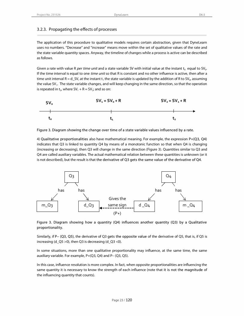
The application of this procedure to qualitative models requires certain abstraction, given that DyneLearn uses no numbers. “Decrease” and “increase” means move within the set of qualitative values of the rate and the state variable quantity spaces. Anyway, the timeline of changes while a process is active can be described as follows. Given a rate with value R per time unit and a state variable SV with initial value at the instant t0 equal to SV0. If the time interval is equal to one time unit so that R is constant and no other influence is active, then after a time unit interval R = d_SV, at the instant t1 the state variable is updated by the addition of R to SV0, assuming the value SV1. The state variable changes, and will keep changing in the same direction, so that the operation is repeated in t2, where SV1 + R = SV2; and so on:

Figure 3. Diagram showing the change over time of a state variable values influenced by a rate.

4) Qualitative proportionalities also have mathematical meaning. For example, the expression P+(Q3, Q4) indicates that Q3 is linked to quantity Q4 by means of a monotonic function so that when Q4 is changing (increasing or decreasing), then Q3 will change in the same direction (Figure 3). Quantities similar to Q3 and Q4 are called auxiliary variables. The actual mathematical relation between these quantities is unknown (or it is not described), but the result is that the derivative of Q3 gets the same value of the derivative of Q4.

Figure 3. Diagram showing how a quantity (Q4) influences another quantity (Q3) by a Qualitative proportionality.

Similarly, if P– (Q3, Q5), the derivative of Q3 gets the opposite value of the derivative of Q5, that is, if Q5 is increasing (d_Q5 >0), then Q3 is decreasing (d_Q3 <0).

In some situations, more than one qualitative proportionality may influence, at the same time, the same auxiliary variable. For example, P+(Q3, Q4) and P– (Q3, Q5).

In this case, influence resolution is more complex. In fact, when opposite proportionalities are influencing the same quantity it is necessary to know the strength of each influence (note that it is not the magnitude of the influencing quantity that counts).

t0 t1 t2

SV1 = SV0 + R SV0 SV2 = SV1 + R

Gives the same sign

Q3

d_Q3 m_Q3

has has

Q4

m _Q4 d _Q4

has has

(P+)

Project No. 231526

/ 120

DynaLearn D6.5

In DynaLearn models this information is not immediately available, so this situation in general leads to ambiguity. The ambiguity leads to three new states in a simulation: the positive proportionality is stronger and causes the influenced quantity to follow it; the two proportionalities have the same strength and the balance is zero; finally, the negative proportionality is the strongest one, so that the derivative of the influenced quantity gets the opposite value of the derivative of the influencing quantity. However it is possible to disambiguate the situation using a correspondence between the derivatives of one of the influencing quantities (e.g. Q5) and of the influenced quantity (Q3). In doing so, the derivative of the influenced quantity (d_Q3) will get the value of the derivative of the influencing quantity (d_Q5) irrespective the value of d_Q4.

The magnitude value of the influenced quantity (Q3) eventually has to change. In this case, the operation is not ‘integration’ (as it may be a monotonic function as multiplication or exponential, for example) but the assignment of a derivative value due to the proportionality. As a rule, with the new derivative value, the quantity magnitude moves within the quantity space upwards or downwards, or stabilizes.

Summarizing,

the quantity Q3 gets a positive derivative (d_Q3 >0) and increases when d_Q2 > 0 and the proportionality is positive (P+); d_Q2 < 0 and the proportionality is negative (P–); the quantity Q3 gets a negative derivative (d_Q3 <0) and decreases when d_Q2 > 0 and the proportionality is negative (P–); d_Q2 < 0 and the proportionality is positive (P+); the quantity Q3 gets a derivative zero (d_Q3 =0) and stabilizes when d_Q2 = 0 and the proportionality is either positive (P+) or negative (P–). When the quantity Q3 is simultaneously influenced by two competing proportionalities (P+ and P–) or by proportionalities with the same sign (either P+ or P–) but with opposite values (one is negative and the other is positive), the outcome of these influences is unknown (that is, the derivative of Q3 can be d_Q3 >0, d_Q3 <0 or d_Q3 =0). Note that, contrary to direct influences, the implementation of proportionalities has nothing to do with the magnitude of the influencing quantities, but only with their derivatives. If the influencing quantity is stable (its derivative is zero), the influenced quantity will not change. Comparing the two mechanisms, it is easy to see that direct influences carry much more information than proportionalities.

The causality flow starts with a process and then may propagate to other parts of the system via proportionalities. An example is given by a situation in which both relations I+ (SV, R) and P– (AV, SV) hold. Given the explanations above, it can be inferred that the flow of causality would move as follows: R ĺ SV ĺ AV. The diagrams above make it clear that, in fact, it is a three steps mechanism: first the derivative of the state variable is influenced by the magnitude of the rate; then integration updates the magnitude value of the state variable (and also creates a new derivative value for the SV, because it starts to increase, decrease or remains stable), and finally the new derivative value of the state variable is propagated to the auxiliary variable via the proportionality.

Finally it is important to note that the mechanisms described in this section are similar to the traditional implementations of System Dynamics (Forrester, 2009). However, as numbers are not used at all in DynaLearn, some relevant aspects are different from the numerical-based simulators (for instance, there is no need to add constants to calibrate the model in DynaLearn). Besides that, qualitative representation of quantities (rates, state variables and auxiliary variables) provide much less variation during the simulations. However, as it will be shown in section 4, qualitative models may express complex system behaviours such as cycles, oscillation and delays, and call the learner’s attention to ‘qualitatively significant states of the system’.

Project No. 231526

/ 120

DynaLearn D6.5

The option for this approach to provide mathematical and causal meaning to qualitative dependencies puts some constrains on how the three different types of quantities (rates, state variables and auxiliary variables) can be used, shown in the table below (Table 3).

Table 3. Constrains on how the three types of quantities can be used in qualitative reasoning modelling.

Quantity type Function Can be influenced by…

Can put influence on… Examples

Rate Represents a process

State variables or Auxiliary variables,

exceptionally by Rates

Only on State variables

Birth rate, Emission rate, Growth rate,

Inflow, Outflow

State variable

Accumulation of the ‘substance’, represents the

state of the system

Rates only Rates or Auxiliary

variables, but not on State variables

Number of, Biomass,

Amount of, Area

Auxiliary variable

Used to represent the effects of the propagation of

processes

State variables or Auxiliary variables,

but not by Rates

Rates or Auxiliary variables but not on

State variables

Density, Pressure,

Volume, Shade

It is also important to note that any quantity, in principle, can be modelled as a state variable or an auxiliary variable. It is a modelling decision. Of course, choosing to represent it as a state variable immediately requires the representation of a rate that would directly influence it, and assume that any change in this variable should be provoked by changes in the rate (and not by changes in the quantity itself).

3.3. Discussion

Causality is a central theme in DynaLearn. This section showed that explicit representation of causality is useful to support learners in acquiring established knowledge about the world. This is done by means of adequate vocabulary to communicate causal relations within systems of interest. Many of the modelling elements available in DyanLearn contribute to implement causal relations in different Learning Spaces.

However, direct influences and proportionalities refine the representation of causality from LS4 onwards. Compared to previous LS, these dependencies bring a new element to the simulations, the mathematical meaning of processes. Measurement of variation and integration after a certain period of time definitely put DynaLearn into the system dynamics arena, by implementing a qualitative system dynamics.

The following section dissects the LS4, 5 and 6 models produced in Tasks 6.2 and 6.4 and characterizes model patterns, pieces of reusable and transferrable model structures that regularly reappear in the models, and that can be further used as the basis for the learning by modelling pedagogical approach of DynaLearn curriculum.

Project No. 231526

/ 120

DynaLearn D6.5

4. Model patterns

Finding patterns in nature is one of the most productive approaches to understanding natural processes and systems. However, defining patterns is not an easy task. According to Pickett et al. (2007), patterns are “repeated events, recurring entities, replicated relationships, or smooth or erratic trajectories observed in time or space” (p.49). Note that in this definition, both the structure and the behaviour of ecological systems are mentioned. When patterns are recognized, they become important elements to anchor theoretical concepts in ecology.

Essential for understanding the behaviour of ecological systems is to understand controlling mechanisms known as feedback loops. This concept refers to the answer of the system’s components to changes in its own size (Odum, 1985). Direct or simple feedback loops involve at least a rate that influences a state variable and is influenced back by this quantity. In contrast, indirect or complex loops involve at least an auxiliary variable that puts the influence into the rate that starts the causal flow. Both types of feedback loops may be, in turn, classified as either positive or negative feedback. By definition, positive feedback tends to reinforce the effect of the process, and negative feedback, also known as a self-correcting or balancing loop, tends to reduce the input that has caused it.

Given that models are abstract representations of natural systems, it is arguably that identifying model patterns, characterized in terms of model structures involving processes and propagation of their effects, may become a powerful tool to transform observations of real systems into models. When it comes to systems behaviour, specific model patterns may also be associated to specific behaviour patterns.

Relevant behaviour patterns in ecological systems include: exponential growth (positive and negative or decay), cyclical behaviours (oscillation, overshoot and collapse), S-shaped behaviour, steady state. Definitions of these behaviours are presented in Appendix F.

The model patterns presented in this section result from the analysis of 94 models produced by WP6 partners in Tasks 6.2 and 6.4, exploring DynaLearn Learning Spaces 4, 5 and 6. Three classes of model patterns are characterized. These patterns intend to represent both the structure and the above described behaviours of ecological systems. Three classes of model patterns are characterized: basic models (six classes), patterns resulting of the combination of basic patterns, and patterns related to the refinement of systems behaviours.

Firstly, basic patterns and relevant variations are organized in six groups and discussed. Among them, patterns that do not include feedback loops, often found in the middle of the system structure, patterns that include feedback loops and patterns that rely on calculations (arithmetic operations) to define the size of a rate.

Secondly, some basic patterns are combined to produce more complex model structures, also associated to more complex behaviours. Finally, the third class of patterns refers to representing specific systems behaviour by means of the addition of constraints (correspondences) to other patterns or the use of exogenous quantities, a facility provided by DynaLearn in which quantities influence the system by exhibiting specific behaviours, but are not influenced by the system (Bredeweg et al. 2007).

These three classes of patterns are discussed in the following sections.

Project No. 231526

/ 120

DynaLearn D6.5

4.1. Basic modelling patterns

4.1.1. A single rate and process

In DynaLearn, any process is associated to a rate, a measure of the variation of the state variable per time unit. However, in some cases two competing processes are aggregated as if they were a single process. In these cases the aggregated process is also represented by a single rate, being the effects of the aggregation captured by the rate’s quantity space.

This section presents the basic pattern of a process, represented by a rate and a state variable. Among the variations of this pattern, positive and negative direct influences, a process that represents the aggregation of competing processes and a single rate that affects two or more state variables.

4.1.1.1. A single rate representing a single process

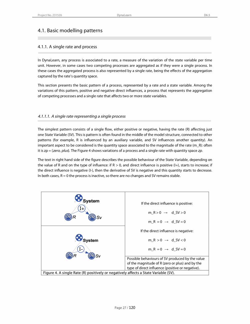
The simplest pattern consists of a single flow, either positive or negative, having the rate (R) affecting just one State Variable (SV). This is pattern is often found in the middle of the model structure, connected to other patterns (for example, R is influenced by an auxiliary variable, and SV influences another quantity). An important aspect to be considered is the quantity space associated to the magnitude of the rate (m_R): often it is zp = {zero, plus}. The Figure 4 shows variations of a process and a single rate with quantity space zp.

The text in right hand side of the figure describes the possible behaviour of the State Variable, depending on the value of R and on the type of influence: if R > 0, and direct influence is positive (I+), starts to increase; if the direct influence is negative (I-), then the derivative of SV is negative and this quantity starts to decrease. In both cases, R = 0 the process is inactive, so there are no changes and SV remains stable.

If the direct influence is positive:

m_R > 0 ĺ d_SV > 0

m_R = 0 ĺ d_SV = 0

If the direct influence is negative:

m_R > 0 ĺ d_SV < 0

m_R = 0 ĺ d_SV = 0

Possible behaviours of SV produced by the value of the magnitude of R (zero or plus) and by the type of direct influence (positive or negative).

Figure 4. A single Rate (R) positively or negatively affects a State Variable (SV).

Project No. 231526

/ 120

DynaLearn D6.5

Examples of uses of this basic pattern includes the ‘water delivery from surface and subsurface runoff’ rate positively influencing the amount of water in a river segment (D6.2.5, Zitek et al. 2010, model ‘Flood protection LS5’), and the deforestation rate, a negative influence removing the vegetation cover.

4.1.1.2. A single rate representing an aggregate of processes

Often competing processes are ‘aggregated’ into a single process, and modelled with a single rate. In these cases, rates of two basic patterns (with positive and negative influences, assumed to be respectively R1 and R2) are aggregated into single rate (R ) with quantity space mzp, representing values {minus, zero, plus}. Accordingly, the values of the rate R express the relationship between R1 and R2, as shown in the following Figure 5.

m_R < 0 ĺ d_SV<0 ( ĺ m_R1 < m_R2)

m_R = 0 ĺ d_SV=0 ( ĺ m_R1 = m_R2)

m_R > 0 ĺ d_SV>0 ( ĺ m_R1 > m_R2)

Rate (R) values both determine the derivative of SV and Possible behaviours of SV and the equivalence with two rates in the correspondent case of single competing processes pattern are shown.

Figure 5. A single Rate (R), with aggregated quantity space (mzp), positively affects a State Variable (SV). R expresses the relationship between two opposite influences, with rates R1 and R2.

As mentioned in the figure, if R = zero, the derivative of SV is also zero and the quantity remains stable. Note that this behaviour can be explained in two ways: either both processes active (R1 = R2 > 0 and the resultant is zero) or inactive (R1 = R2 = 0). This way, some information about the actual behaviour of the system is lost as a consequence of aggregating processes, and additional information is required in order to solve this uncertainty. Note also that the positive and negative values of the rate R can be arbitrarily associated respectively to a flow from the LHS to the RHS (inflow) and to a flow from the RHS to the LHS (outflow) and vice-versa (see below).

Among the models produced by DynaLearn project, the aggregated rate was used to represent the occupation rate of a local metapopulation, as a combination of colonization and local extinction processes (D6.4.1, Salles et al. 2011).

Project No. 231526

/ 120

DynaLearn D6.5

4.1.1.3. A process with multiple influences

Another variation of the single process pattern involves one rate (R) influencing two or more state variables (SV1, SV2). Assuming that R has quantity space with values {minus, zero, plus}, the possible behaviours of SV1 and SV2 are described in the Figure 6.

m_R > 0 ĺ d_SV1 > 0 AND d_SV2 < 0

m_R = 0 ĺ d_SV1 = 0 AND d_SV2 = 0

m_R < 0 ĺ d_SV1 < 0 AND d_SV2 > 0

Possible behaviours of SV1 and SV2 produced by the basic pattern shown in the figure aside

Figure 6. Basic pattern in which a single Rate (R) affects two State Variables (SV1, SV2).

The pattern presented in the figure above can be used to represent the transfer of a substance from one place (via I-) to another (via I+). If the R quantity space is {zero, plus}, then the active process creates a unidirectional flow of the substance. However, if R quantity space is {minus, zero, plus}, the model pattern can represent a flow in both directions, as if something is removed from one place and taken to another one and then, with R < 0, moving the thing back to the initial position.

For example, consider the migratory movement of coral reefs between northern locations and the Equator. The aggregated single rate (Dispersal rate) with quantity space {toward equator, zero, from equator}, represents the competing processes emigration and immigration between different locations (D6.4.4, Leiba et al. 2011, model ‘Coral reef distribution’).

4.1.2. Two or more processes affecting a single state variable

This basic pattern consists of a state variable influenced by two competing processes (with rates R1 and R2), as shown in the Figure 7. In this case, it does not matter if the quantity space of R1 and R2 is zp or mzp, the resultant system behaviour depends only on the relative size of the rates’ magnitudes. Note that this pattern does not include a feedback loop.

m_R1 > m_R2 ĺ d_SV > 0

m_R1 = m_R2 ĺ d_SV = 0

m_R1 < m_R2 ĺ d_SV < 0

Resultant SV derivative (d_SV) according to relative size of the rates magnitude of

competing processes Figure 7. Two competing rates (R1, R2) influencing one State variable (SV).

Project No. 231526

/ 120

DynaLearn D6.5

An example of this pattern can be found in D6 2.5 (Zitek et al. 2010, model ‘Sediment transport LS4’) to represent the effects of the sediment input rate and sediment output rate in a river segment.

4.1.3. Network of causal influences

Often a linear chain of causality propagates the effects of processes to other parts of the system. As mentioned in section 3, propagation of causality is implemented by means of qualitative proportionalities linking a state variable to one or more auxiliary variables or rates.

In this section, branching, a variation of network of causal influences pattern, is discussed. IN this case, two or more lines of causality are created from a state variable or an auxiliary variable. Note that feedback loops are not considered in these patterns.

Other interesting variations - the short chain, consisting of a single auxiliary variable or a rate following the state variable; and the long chain, with two or more auxiliary variables – are discussed in the Appendix C.

4.1.3.1. Network of influences – short chain

The Figure 8 shows the simplest network for propagating the effects of processes to auxiliary quantities: an auxiliary variable influenced by the state variable. The influencing processes are not shown in the Figure 8

d_SV > 0 ĺ d_AV > 0

d_SV = 0 ĺ d_AV = 0

d_SV < 0 ĺ d_AV < 0 Possible behaviours of AV produced by the propagation of SV behaviour.

Figure 8. Propagation of the effects of process affecting a state variable (SV) to an auxiliary variable (AV)

Some possible variations in this short chain include alternative sign (negative) in the proportionality and a rate replacing the AV, so that another process would be influenced by the SV. An example can be found in model ‘Sediment transport LS4’ (D6.2.5, Zitek et al. 2010), in which the amount of sediment in the river segment influences (P+) the height of river bottom.

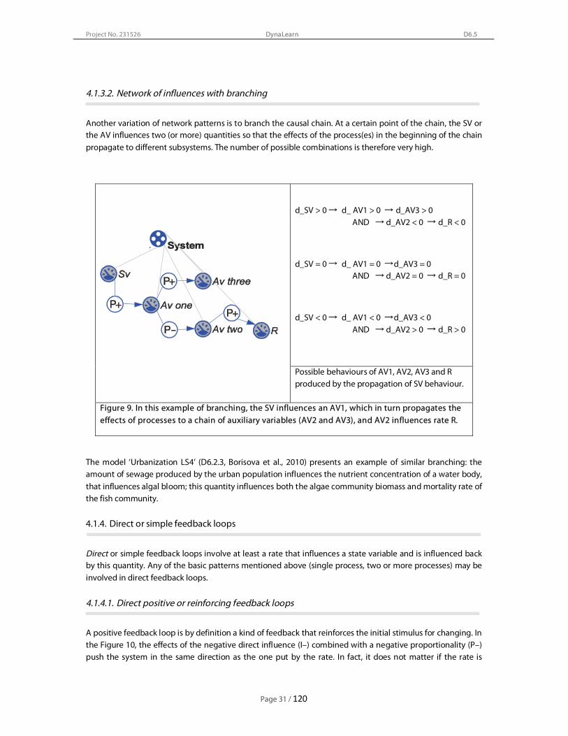
Project No. 231526

/ 120

DynaLearn D6.5

4.1.3.2. Network of influences with branching

Another variation of network patterns is to branch the causal chain. At a certain point of the chain, the SV or the AV influences two (or more) quantities so that the effects of the process(es) in the beginning of the chain propagate to different subsystems. The number of possible combinations is therefore very high.

d_SV > 0 d_ AV1 > 0 d_AV3 > 0 AND d_AV2 < 0 d_R < 0

d_SV = 0 d_ AV1 = 0 d_AV3 = 0 AND d_AV2 = 0 d_R = 0

d_SV < 0 d_ AV1 < 0 d_AV3 < 0 AND d_AV2 > 0 d_R > 0

Possible behaviours of AV1, AV2, AV3 and R produced by the propagation of SV behaviour.

Figure 9. In this example of branching, the SV influences an AV1, which in turn propagates the effects of processes to a chain of auxiliary variables (AV2 and AV3), and AV2 influences rate R.

The model ‘Urbanization LS4’ (D6.2.3, Borisova et al., 2010) presents an example of similar branching: the amount of sewage produced by the urban population influences the nutrient concentration of a water body, that influences algal bloom; this quantity influences both the algae community biomass and mortality rate of the fish community.

4.1.4. Direct or simple feedback loops

Direct or simple feedback loops involve at least a rate that influences a state variable and is influenced back by this quantity. Any of the basic patterns mentioned above (single process, two or more processes) may be involved in direct feedback loops.

4.1.4.1. Direct positive or reinforcing feedback loops

A positive feedback loop is by definition a kind of feedback that reinforces the initial stimulus for changing. In the Figure 10, the effects of the negative direct influence (I–) combined with a negative proportionality (P–) push the system in the same direction as the one put by the rate. In fact, it does not matter if the rate is

Project No. 231526

/ 120

DynaLearn D6.5

associated to quantity space zp or mzp. The effect is the same – a reinforcement on the initial stimulus. The figure below shows an example of a rate with quantity space mzp.

m_R > 0 ĺ d_SV < 0 ĺ d_R > 0 ĺ m_R > 0

m_R = 0 ĺ d_SV = 0 ĺ d_R = 0 ĺ m_R = 0

m_R < 0 ĺ d_SV > 0 ĺ d_R < 0 ĺ m_R < 0

Possible behaviours of SV according to the possible values of R; the propagation of the derivative of SV, to the derivative of R causes the rate to change in the same direction as SV, increasing the initial stimulus on SV. When R is zero, the whole chain becomes stable.

Figure 10. A positive direct feedback loop involving a negative direct influence and a negative proportionality.

Model ‘Increase of flood risk due to deforestation’ (D6.2.5, Zitek et al. 2010) includes a direct feedback as shown in the figure above: Deforestation rate (mzp) puts a direct negative influence on the amount of forest, and is influenced via a positive proportionality by the state variable.

A variation of this pattern is obtained if direct influence and proportionality have positive signs. However, if the influences have opposite signs, a negative feedback loop is created. Examples are given in the following section.

4.1.4.2. Direct negative feedback loops

The Figure 11 shows a pattern involving two processes that put influences in the same SV, and this quantity in turn puts influences on both rates. For the sake of simplicity, suppose the two rates R1 and R2 are associated to quantity spaces zp.

Project No. 231526

/ 120

DynaLearn D6.5

m_R1 > m_R2 ĺ d_SV > 0 ĺ d_R1 < 0 AND ĺ d_R2 > 0

m_R1 = m_R2 ĺ d_SV = 0 ĺ d_R1 = 0 AND ĺ d_R2 = 0

m_R1 < m_R2 ĺ d_SV < 0 ĺ d_R1 > 0 AND ĺ d_R2 < 0

Possible behaviours of SV according to the comparison of R1 and R2 values; the propagation of d_SV to the derivatives of the two rates causes d_R1 to change the opposite direction due to the negative proportionality, and d_R2 to change in the same direction due to the positive proportionality. As a result both rates change so that the smaller one increases, and the bigger one decreases. The resultant is a decreasing in the initial stimulus on SV bringing this quantity to a balance. When R is zero, the whole chain becomes stable.

Figure 11. A double negative direct feedback loops involving pairs of direct influence and proportionality with opposite signs.

A number of variations in the double feedback pattern are possible, including an alternative combination of negative loops; a positive and a negative loop; both positive loops. Another source of variation may involve the number of active processes influencing SV, creating multiple feedback loops, and a number combination of positive and negative loops.

An example of double feedback loop, with a positive and a negative loops, is presented in D6.2.2 (Noble, 2010) in which the model ‘Climate change LS4’ includes a fish population with birth and death rates influencing population size respectively with positive and negative direct influences, and size puts proportionalities back to the rates, creating a positive loop with birth rate, and a negative loop with death rate.

All in all, these relations bring great complexity to the system. Probably this is the most common situation found in the environment, where typically “everything is connected to everything”.

4.1.5. Indirect or delayed feedback

In some cases, a causal chain propagates the effects of the process into a network of causal relations, before the feedback mechanism starts to operate. These are named indirect or delayed loops, that may be short, when the state variable influences an auxiliary variable which in turn influences the rate, or long, when two or more auxiliary variables propagate the effects of a process until an auxiliary variable puts the feedback loop on the rate. As in previous cases, balancing or reinforcing results may be achieved by this type of loops.

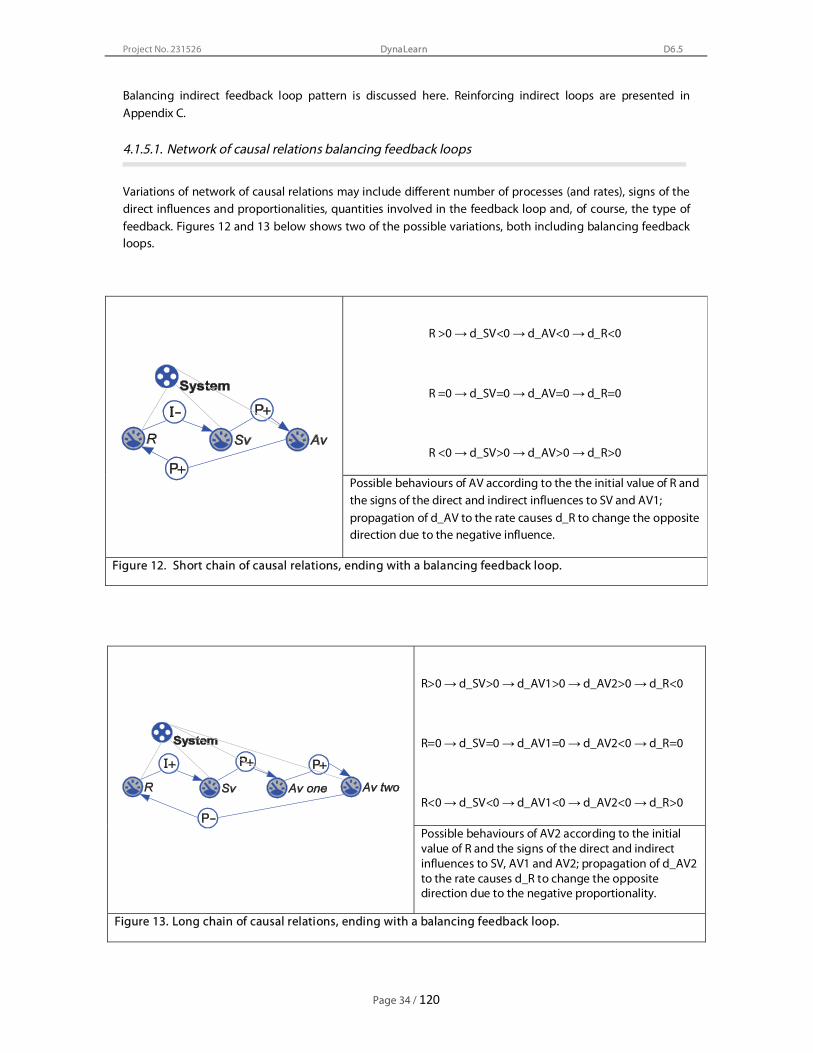
Project No. 231526

/ 120

DynaLearn D6.5

Balancing indirect feedback loop pattern is discussed here. Reinforcing indirect loops are presented in Appendix C.

4.1.5.1. Network of causal relations balancing feedback loops

Variations of network of causal relations may include different number of processes (and rates), signs of the direct influences and proportionalities, quantities involved in the feedback loop and, of course, the type of feedback. Figures 12 and 13 below shows two of the possible variations, both including balancing feedback loops.

R >0 ĺ d_SV<0 ĺ d_AV<0 ĺ d_R<0

R =0 ĺ d_SV=0 ĺ d_AV=0 ĺ d_R=0

R <0 ĺ d_SV>0 ĺ d_AV>0 ĺ d_R>0

Possible behaviours of AV according to the the initial value of R and the signs of the direct and indirect influences to SV and AV1; propagation of d_AV to the rate causes d_R to change the opposite direction due to the negative influence.

Figure 12. Short chain of causal relations, ending with a balancing feedback loop.

R>0 ĺ d_SV>0 ĺ d_AV1>0 ĺ d_AV2>0 ĺ d_R<0

R=0 ĺ d_SV=0 ĺ d_AV1=0 ĺ d_AV2<0 ĺ d_R=0

R<0 ĺ d_SV<0 ĺ d_AV1<0 ĺ d_AV2<0 ĺ d_R>0

Possible behaviours of AV2 according to the initial value of R and the signs of the direct and indirect influences to SV, AV1 and AV2; propagation of d_AV2 to the rate causes d_R to change the opposite direction due to the negative proportionality.

Figure 13. Long chain of causal relations, ending with a balancing feedback loop.

Project No. 231526

/ 120

DynaLearn D6.5

As discussed previously, network patterns appear when propagation of the effects of processes and create connections with other subsystems (patterns) and distant feedback loops, which adds great complexity to the models.

The model ‘Pollination’ (D6.4.1, Salles et al. 2011) illustrates the use of this pattern: the amount of seeds produced by the trees influences (P+) the farmers’ revenue, that influences investment (P+), which influences (P+) the agricultural production. Here the chain branches into deforestation rate (P+) and pesticide use (P+). These quantities influence respectively seed mortality rate (via number of trees) and pollination rate (via number of bees). Altogether, both processes have a balacing effect on the total feedback loops.

4.1.6. Inequality reasoning in unbalanced situations

DynaLearn provides a functionality that allows for qualitative arithmetic operations of addition and subtraction, and is useful to support inequality reasoning. Combined to qualitative proportionalities, the magnitude value of a third quantity (often a rate) can be calculated based on comparisons between magnitudes of auxiliary variables. This mechanism serves also to start changes in the system (when the situation is unbalanced) and stop such changes (when the system reaches the equilibrium).

This basic pattern accepts a number of variations, being the most useful for the models produced in DynaLearn Tasks 6.2 and 6.4 the use of subtraction of unbalanced pairs of influences. This section presents an example of the use of subtraction for calculating rates, with feedback loops.

Another example of the use of subtraction for calculating rates without feedback loops is presented in the Appendix C.

4.1.6.1. Calculating flows in unbalanced situations with feedback

Arithmetic calculations associated to feedback patterns create a powerful pattern that represents how an unbalanced situation leads to the dynamic equilibrium (Figure 14). As above, it is assumed that the subtraction operation is (m_AV1 – m_AV2 = R], and the quantity space associated to the rate is mzp.

Project No. 231526

/ 120

DynaLearn D6.5

m_AV1 > m_AV2 ĺ m_R > 0 ĺ d_SV1 < 0 ĺ d_AV1 < 0 AND ĺ d_SV2 > 0 ĺ d_AV2 > 0

m_AV1 = m_AV2 ĺ m_R = 0 ĺ d_SV1 = 0 ĺ d_AV1 = 0 AND ĺ d_SV2 = 0 ĺ d_AV2 = 0

m_AV1 < m_AV2 ĺ m_R < 0 ĺ d_SV1 > 0 ĺ d_AV1 > 0 AND ĺ d_SV2 < 0 ĺ d_AV2 < 0

Behaviour is triggered by the comparison between two auxiliary variables (AV1 and AV2); inequality leads to an unbalanced situation that initiates the mechanism that leads to the equilibrium. If m_AV1 = m_AV2, the system is in equilibrium.

Figure 14. Two competing proportionalities coming from auxiliary variables (AV1 and AV2) affect a rate (R), being its value calculated by a qualitative subtraction: (m_AV1 – m_AV2 = R]. The rate influences two state variables (SV1 and SV2) and then the changes propagate to AV1 and AV2, via feedback loops, and may change again the value of the rate.

The analysis above shows that if in the initial situation m_AV1 > m_AV2 holds, then the causal chain leads to d_AV1 < 0, which makes m_AV1 to decrease, and d_AV2 > 0, which makes m_AV2 to increase. This way, the situation changes to a balance, when m_AV1 = m_AV2 and rate R=0, stopping the whole mechanism. Note that the value zero does not mean that the two processes are inactive (see the pattern described in section 1.1.1.3 ‘A process with multiple influences’). In fact, they must be active, but in balance: output cancels input. Similar mechanism operates when m_AV1 < m_AV2 holds.

An example of this pattern is found in model ‘Metapopulation – Levins model’ (D6.4.1, Salles et al. 2011). The subtraction (colonization – extinction = occupation rate], and the rate influences negatively available patches, which influences (P+) colonization. The rate also positively influences occupied patches, which in turn influences (P+) extinction. As the rate has quantity space mzp, when colonization > extinction, occupation rate is positive and the propagation of the process to other quantities result in an equilibrium so that colonization and extinction stabilizes in low, and occupied patches stabilizes in high. If the colonization < extinction, the rate is negative, and the system tends to collapse, with occupied patches decreasing in low, and available patches to increase in high.

Variations of this pattern may include more auxiliary variables between the state variables and the AVs that calculate the value of R; the possible qualitative values of the rates; increasing the number of processes (Rs and SVs), the type of feedback loops and others. All these changes give an idea of the magnitude of variation in this pattern.

Project No. 231526

/ 120

DynaLearn D6.5

4.2. Combined patterns

The following patterns are complex representations created by the combination of the previous basic patterns or variations of these patterns.

In fact, complex behaviour observed in natural phenomena, such as oscillations and cycles, cannot be produced by basic patterns discussed above. The possibility of combining patterns is an answer to this limitation. In this section some of these combinations are presented.

4.2.1. Two connected single aggregated processes

Often population models are organized around an aggregated process (growth process, in which birth and death rates are replaced by a growth rate with quantity space mzp). When two of these aggregated processes are combined, models of interactions between two populations can be successfully implemented (Figure 15). For example, this combined pattern was used by Correa (2011) to represent competition between two populations of algae, the Cyanophyceae and a functional group that represent other algae species found in the same lake, and to represent the predator-prey system, involving algae and herbivores populations.

Figure 15. Left: Two single rate for process aggregated processes connected by a short chain network; and right: Typical behaviour produced by the combined pattern presented aside.

4.2.2. Double two processes patterns connected by network branching

Interactions between two populations can be implemented with explicit representations of natality and mortality. IN this case, following the famous Lotka-Volterra models (for ex., Gotelli, 1995) auxiliary variables are included between the two populations to represent the effects of one population on the other one, and vice-versa. Figure 16 presents a combined pattern resulting of two basic patterns, each with two processes influencing a single state variable connected by a branching network chain. This combined pattern set up was used by Salles et al. (2003) to model interactions between populations of two species.

Project No. 231526

/ 120

DynaLearn D6.5

Figure 16: A complex model connected resulting of two subsystems, each with two processes influencing a single state variable, connected via network branching, adapted from Salles et al. (2003). Left: Typical behaviour exhibited by the model pattern presented aside

4.2.3. Pattern involving double inequality reasoning patterns

Inequality reasoning provides a very productive modelling pattern that brings together processes affecting two state variables that interact each other via network chain patterns. In this case, an interesting behaviour emerges, namely the oscillation of the two state variables that cycle with a time lag separating them (Figure 17). An example also exploring the Lotka-Volterra predator – prey population model is presented in deliverable D6.4.5 (Zitek et al. 2011).

Figure 17. Left: Combined pattern resulting of two inequality reasoning basic patterns connected via short network chain; and right: Typical behaviour exhibited by the model pattern presented aside.

Project No. 231526

/ 120

DynaLearn D6.5

4.3. Refining behaviour patterns

Some specific model patterns create system behaviour patterns of interest, and as such are included in this section. However, in order to obtain the desired behaviour, different DynaLearn modelling elements may be used: exogenous quantities (Bredeweg et al. 2007), correspondences and conditional knowledge. Exogenous behaviour quantities may exhibit specific behaviours, that may be used to isolate (keeping quantity magnitude values constant and/or their derivative values steady) during a simulation or to produce complex behaviours (such as sinusoidal oscillation). Correspondences and conditional knowledge are also useful to remove certain undesired behaviours.

4.3.1. Exogenous quantity patterns

While complex system behaviour poses important requirements to be obtained with the patterns describe so far, DynaLearn offers the possibility of starting a simulation with quantities that exhibit built in specific behaviours, defined outside the system, the so called exogenous behaviours (Bredeweg et al., 2007). In DynaLearn LS6 exogenous behaviours of selected quantities may affect their magnitude and / or their derivatives. The following two exogenous behaviours may affect the magnitude of a quantity: generate all values and constant. And the following seven exogenous behaviours may affect the derivative of a quantity: increase, steady, decrease, parabola (positive), parabola (negative), sinusoidal and random. Exogenous behaviour can only be applied in the initial scenario to quantities that are not affected by any other quantity. These exogenous quantities may transfer the behaviour to other quantities (state variables, rates or auxiliary variables) and in doing so, they influence the system behaviour. The Appendix F presents a detailed description of the simulations starting with the exogenous behaviours.

Effects of exogenous quantities on the simulations are remarkable. In DynaLearn LS2 and LS3, simulations are driven by assigning the derivative of selected quantities one of the (exogenous) behaviours increase, steady or decrease. In LS4 and LS5, simulations may start with active processes (m_R>0) but the same types of exogenous behaviour are available (increase, steady or decrease). In LS6 DynaLearn all the nine exogenous behaviour patterns are available.

Figure 18 shows an example of exogenous behaviour (parabola negative).

Figure 18. Initial scenario of a simple model, in which the “Exogenous quantity” has assigned the negative parabola behaviour, shown on the RHS.

Project No. 231526

/ 120

DynaLearn D6.5

Some of the exogenous behaviour are of great value for model development, others produce complex behaviour that can produce simulations representing important ecological and environmental science phenomena. Included in the first group are exogenous increase and decrease that can be used to test the behaviour of long chains of causality, before introducing processes. The possibility of using the exogenous steady is quite important to isolate part of the system and in doing simplify simulations with high degree of complexity.

Exogenous parabola (positive and negative), sinusoidal and random behaviours in turn add great complexity to the simulation, and easily the number of states produced goes far beyond manageable limits. These are still powerful instruments to capture complex behaviour, at the cost of ignoring the initial cause of change in the system.

A number of complex models developed in Task 6.4 depend on exogenous quantities to start the simulations. Among others, ‘Metapopulation Hanski Integrated approach’ model (cf. D6.4.1, Salles et al., 2011) and ‘Intraspecific population regulation LS6’ model (cf. D6.4 2, Noble and Cowx, 2011).

4.3.2. Modelling with correspondences and conditional knowledge

Correspondences are directly associated to the behaviour of the system, as the quantities show the same state in all possible values (Q-correspondence) or in some of the possible values (V-correspondence). As such, they are not understood in this work as being ‘modelling patterns’, but certainly are important elements to restrict the behaviour generated by the model and, this way, reduce ambiguity and get the exact behaviour wanted in a simulation.

To start with a single example, the simplest model on population dynamics is based on the pattern ‘double direct feedback loop’ presented in section 4.1.4. If the quantities birth rate and death rate have not the value zero when number of individuals is zero, the simulation would produce a biologically impossible situation: the existence of natality or mortality when the population does not exist. In this case, the use of V-correspondences between these three values is compulsory. In other words, to capture the correct behaviour of a single population, correspondences have to be included in one of the model patterns.

A more interesting example is given in models aiming to produce the famous (for biologists) ‘S-shaped behaviour’. In ecology, the logistic equation has played an important role in implementing the interaction between two laws (exponential growth and limits to growth) to produce a strong sigmoidal pattern showing population trends determined by the influence of resource availability on the abundance of organisms, the ‘density dependence’ condition (cf. Dodds, 2009; Gotelli, 1995, among others).

In this context, the variable representing population size has two limit points, where the system behaviour change: K, the carrying capacity, in which the state variable stabilizes, and K/2, the inflection point.

The model is implemented in DynaLearn LS64, and consists of eight model fragments. Two model fragments (MF01 and MF02e) are shown in the Figure 9: ‘MF01 Population configuration’ and ‘MF02e Number of individuals equal to carrying capacity (K)’.

4 A preliminary version of this model was produced by Floris Linnebank, to whom we would like to thank for the fruitful discussions that resulted in the present model (and in many other topics) and it can be found with more details in the Appendix F!

Project No. 231526

/ 120

DynaLearn D6.5

Figure 19. Left: Model Fragment “MF01 Population configuration”; and right: model fragment “MF02e Number of individuals equal to carrying capacity”.

MF01 shows clearly the importance of value correspondences (Table 4):

Table 4. Value correspondences between quantity spaces of Number of (individuals) and Net (Growth) rate.

Number of (individuals) Net (growth) rate

zero zero

below inflection point plus

inflection point plus

above inflection point plus

K zero

above K minus

In this model, the use of conditional knowledge is essential to assure the simulation produces the expected behaviour, which heavily depends on combinations of magnitudes and derivatives of all the quantities. The Table 5 below shows how the conditional knowledge was applied:

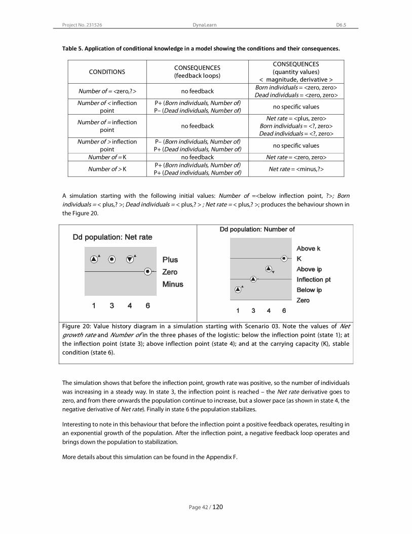
Project No. 231526

/ 120

DynaLearn D6.5

Table 5. Application of conditional knowledge in a model showing the conditions and their consequences.

CONDITIONS CONSEQUENCES (feedback loops)

CONSEQUENCES (quantity values)

< magnitude, derivative >

Number of = <zero,?> no feedback Born individuals = <zero, zero> Dead individuals = <zero, zero>

Number of < inflection point

P+ (Born individuals, Number of) P– (Dead individuals, Number of) no specific values

Number of = inflection point no feedback

Net rate = <plus, zero> Born individuals = <?, zero> Dead individuals = <?, zero>

Number of > inflection point

P– (Born individuals, Number of) P+ (Dead individuals, Number of) no specific values

Number of = K no feedback Net rate = <zero, zero>

Number of > K P+ (Born individuals, Number of) P+ (Dead individuals, Number of) Net rate = <minus,?>

A simulation starting with the following initial values: Number of =<below inflection point, ?>; Born individuals = < plus,? >; Dead individuals = < plus,? > ; Net rate = < plus,? >; produces the behaviour shown in the Figure 20.

Figure 20: Value history diagram in a simulation starting with Scenario 03. Note the values of Net growth rate and Number of in the three phases of the logistic: below the inflection point (state 1); at the inflection point (state 3); above inflection point (state 4); and at the carrying capacity (K), stable condition (state 6).

The simulation shows that before the inflection point, growth rate was positive, so the number of individuals was increasing in a steady way. In state 3, the inflection point is reached – the Net rate derivative goes to zero, and from there onwards the population continue to increase, but a slower pace (as shown in state 4, the negative derivative of Net rate). Finally in state 6 the population stabilizes.

Interesting to note in this behaviour that before the inflection point a positive feedback operates, resulting in an exponential growth of the population. After the inflection point, a negative feedback loop operates and brings down the population to stabilization.

More details about this simulation can be found in the Appendix F.

Project No. 231526

/ 120

DynaLearn D6.5

4.4. Discussion on patterns

The idea of generic and transferable model structures for introducing system dynamics and systems thinking in education has been discussed by system dynamics community (Forrester, 1997; Richmond, 2001). Forrester (1997) argues that some generic structures can be found repeatedly in different situations, even in entirely different domains of knowledge. For this author, if a particular structure is understood in one setting, it is understood in all settings. This way, these generic structures “provide the student with power to move between subjects with the learning on one subject being applied to other subjects. After understanding a collection of basic dynamic structures, a student can quickly draw on one to understand a new situation if its structure has been encountered previously” (Forrester, 1997, p. 24).

A similar concept has been independently developed by WP6 partners to characterize and identify qualitative model patterns while analyzing the results of Task 6.2 and 6.4 and preparing Task 6.5. Both approaches share the notion of a piece of model that can be reused, and are valuable tools for learning. Among the differences, the idea that generic structures are actually small system dynamics models, used as stand-alone models or as subsystems of bigger models (Richmond 2001). Qualitative model patterns in turn include micro and partial patterns, as in network chains, that are bridging structures for linking different patterns. Besides that, qualitative model patterns use only qualitative representations of differential equations and monotonic functions, and use correspondences and conditional knowledge for overcoming some of these restrictions in order to obtain some behaviors of interest. Of course, numerical generic structures may easily create behaviours such as exponential growth, damping and precise notions as half-life. Qualitative representations in turn present explicit accounts of causality, may be used with incomplete knowledge and provide a rich vocabulary for using an appropriate language in the educational environment.

This section presented three categories of model patterns: basic patterns, combination of basic patterns and refinements of behaviour patterns. These model patterns are associated to specific systems behaviour, as they are in general found among ecological systems. Examples of occurrences of these patterns in Task 6.2 and 6.4 models were referred.

Simple patterns based in single processes and one rate (section 4.1.1), or two processes acting on a state variable (section 4.1.2) generate the following behaviours: increase, decrease and stable that may propagate to other parts of the system (section 4.1.3). Direct and indirect feedback loops involving just one state variable result in more complex and realistic models. Reinforcement (positive) loops increase the tendency of growth, and balancing (negative) loops bring the system to dynamic equilibrium point. However, these patterns also produce the same system behaviours - increase, decrease and stable (sections 4.14 and 4.1.5).

Combinations of basic model patterns result in more complex patterns, and in more complex behaviours. Three of these patterns were presented, all of them including two state variables that interact, and both controlled by negative feedback loops. The result is the oscillation pattern, due to their similar structure, control mechanism and interaction (Chung, 1994). Experiments with the same pattern but positive feedback loops resulted in increase and decrease patterns only, an expected behaviour according to Chung (1994).

Complex system behaviours can be induced into the system of interest by using exogenous quantities (section 4.3.1), and the use of correspondences allow for complex behaviour, such as a qualitative version of the S-shaped curve, that results from a shift between positive feedback into a negative feedback loop (section 4.3.2).

Having prepared a toolbox of model patterns, next section discusses how these building blocks can be used in learning by modelling activities in DynaLearn.

Project No. 231526

/ 120

DynaLearn D6.5

5. Towards a qualitative system dynamics based curriculum for DynaLearn

An important aspect of the DynaLearn curriculum is to answer the following question: taking a systems view on environmental science, how to develop skills and competences that are actually useful for a learning by modelling approach?

Previous work in Tasks 6.2 and 6.4 discussed and WP7 evaluated, from the conceptual view, how DynaLearn could support the development of competences and skills established in national educational systems from Brazil and Great Britain (D6.1, Salles et al, 2009), Israel (D7.1, Mioduser et al., 2010) and Austria (D6.4.5, Zitek et al., 2011).

Four sets of competences and skills were brought for discussions as possible guidelines for the LbM approach: (a) the Brazilian approach adopted by FUB for selecting students at the end of secondary school; (b) the United Kingdom competences for A-levels (both in D6.1, Salles et al. 2009); (c) the scientific reasoning skills brought up by TAU (D7.1, Mioduser et al., 2010); and (d) Austrian competence matrix for environmental education (D6.4 5, Zitek et al., 2011).

However, these competences and skills mentioned above are more related to the learner’s cognitive development and acquisition of conceptual domain knowledge. The question to be answered in Task 6.5 and presented in this Deliverable is – how to abstract the essence of the work done in WP6 and WP7 and transfer it into a curriculum proposal that explores the potential of DynaLearn and is generic enough to be applied in other domains beyond environmental science?

Overall results of evaluation activities carried on by WP7 and summarized in D7.2.6 (Mioduser et al. 2011) and D7.4 (Mioduser et al. 2012), showed that exploring and building qualitative models in DynaLearn support the development of concepts in environmental science and motivate the learners to develop their own models with autonomy. Moreover, these studies show that DynaLearn promotes the acquisition of systems thinking skills. It is an important result, as it opens new opportunities for exploring features in DynaLearn environmental science curriculum that may be applicable to different domains. Maybe such opportunities can be explored to reduce the gap between qualitative reasoning and numerical system dynamics modelling while focussing in a common goal: the development of systems thinking skills.

5.1. Systems thinking

According to Caulfield and Maj (2001), “systems thinking is a way of thinking that focuses on the relationships between the parts forming a purposeful whole”. Although a simple definition, the authors argue that system thinking extended its bases on a number of fields and has been practiced in accordance to a number of methodologies. However, a special case has to be made in favour of System Dynamics. This approach, continue Caulfield and Maj (2001), “is concerned with building computer models of complex problem situations and then experimenting with and studying the behaviour of these models over time”.

In this project we defend the idea that DynaLearn offers a modelling workbench for a qualitative system dynamics (QSD), and that learners who used the software improved their abilities in systems thinking. In fact, “students' system thinking and ability to represent a system's structural and behavioural features were contributed by the work with DynaLearn. Along the learning processes, growth of skills and abilities was observed.” (Mioduser et al., 2012, Deliverable D7.4)

Project No. 231526

/ 120

DynaLearn D6.5

And which skills may be related to systems thinking?

5.1.1. System thinking skills

Barry Richmond (1993) presents what are, in his view, seven systems thinking skills: that are commented below:

• Dynamic thinking, that means the ability to see and deduce behaviour patterns rather than focusing on, and seeking to predict, events. A good exercise for developing this skill is to find in texts (books, newspapers and magazines, scientific articles) the modelling elements used to build models and recognize model patterns to associate structure to behaviour.

• Closed-loop thinking: when exercising closed-loop thinking, people will look to the loops themselves (i.e., the circular cause-effect relations) as being responsible for generating the behaviour patterns exhibited by a system. This task is facilitated by the use of model patterns.

• Generic thinking: applies to apprehending the similarities in the underlying feedback-loop relations that generate specific occurrences in different domains. To develop generic thinking skills, people can work with a series of generic structures (model patterns) that progress from simple exponential growth and decay, through S-shaped growth, to overshoot/collapse and oscillation.

• Structural thinking is one of the most rigorous tracks of systems thinking. People need to think carefully about units of measure and adherence to physical conservation laws in the domain being studied. This type of thinking emphasizes the distinction between a state variable and rates.

• Operational thinking means thinking about how things really work; this skill can benefit from causal models as simplified implementation and simulation of complex mechanisms in DynaLearn.

• Continuum thinking means finding ways between the "black and white" extremes. The development of continuum thinking emphasizes the ability to recognize familiar in what appears diverse or distinct. The qualitative reasoning approach, focussing on aspects that distinguish specific qualitative states of the system contributes to refine the learners’ perception of distinct features of the system.

• Scientific thinking has more to do with quantification than measurement”, particularly quantification of things that are not measurable. This is typically the situation in which qualitative models can make a difference. “Thinking scientifically also means being rigorous about testing hypotheses”. Given the facilities provided by DynaLearn and the toolbox consisting of model patterns, create representations for alternative hypotheses can be significant part of the learning by modelling approach taken by DynaLearn curriculum.

5.2. Natural and formal languages in the curriculum

Forrester (2009) points out that a major benefit from building models is the ability of translating concepts from natural language into formal statements required for building computer models. This process can be surprisingly demanding. However, this promotes learning precision in thinking. Also fruitful is what is called

Project No. 231526

/ 120

DynaLearn D6.5

‘reverse translation’, in which translation from formal simulation models language into natural language yields clear statements that embody the precision required to build and use the model (Forrester, 2009).

Exploring texts in natural language to identify entities, quantities and processes was described in evaluation activities run in DynaLearn (for, ex., D7.2.1 by Salles et al. 2010). For the curriculum development, it is important to associate natural language elements to modelling primitives. This way, processes are associated to verbs, actions; entities, to nouns; properties of the entities are associated to nouns describing collections (as population), amounts and scales (volume, mass, amount, height); quantity values, to grade adjectives (as small, large, high); and so on. An example is presented in the following text: ‘Evaporation (process) of water contained in the container (entities) has caused the volume (noun describing amount) of liquid water to decrease up to small (grade adjective).’

During evaluation activities, it was also noted an improvement on the natural language usage with respect to domain knowledge, after learners explored models built in DynaLearn (for example, deaf students in a systems thinking exercise described in D7.3.1, by Salles et al. 2012).

First, from our experience, confirmed during the evaluation activities developed in WP7, it is important for the learner to master the software functionalities and the modelling language. The qualitative system dynamics language is based on few elements but requires a lot of abstraction. However while it is clear that DL curriculum cannot be developed if the modelling language is not fully understood, it is also clear that the language may be presented and discussed in steps.

Learning the modelling language should be referenced to natural language, so that the learner could identify in textbooks, lessons and other sources such as newspapers and the media, systems, processes, rates, feedback loops, see Appendix E.

5.3. Key points for learning by modelling Qualitative System Dynamics

A set of key points for organizing learning activities centred on the learners (and not on the teachers) following a learning by modelling approach is discussed in this section. These point address some rules for handling processes, rates, state variables, direct influences, proportionalities in a way that preserves the conceptual integrity of models and simulations produced by using modelling patterns.

5.3.1. (A) State variables define the state of the system

State variables completely describe the system conditions: as they are directly influenced by processes, state variables are the most important quantities to define the dynamics of the system. When processes are inactive, their values remain stable, and the rates have value zero. In general, auxiliary variables and rates have their values calculated from the state variables. It is also possible that auxiliary variables or even rates become the focal point of the model. For ex. the effects of different influences on growth rate are the most important result obtained in a metapopulation model (D6.4.1, Salles et al. 2011). Anyway, state variables are the quantities that effectively define the state of the system.

State variables are accumulations: State variables (or stocks or levels) are quantities that accumulate over time, or better saying it, they accumulate the effects of the process (via the integration, see section 3.2.2).

Project No. 231526

/ 120

DynaLearn D6.5

Therefore they are more intuitive and easily understood by learners than rates. As put by Forrester, “nowhere in nature does nature take a derivative. Nature only integrates, that is, accumulates.” (Forrester, 1997, p. 27).

State variables are changed only by rates: in QSD, state variables cannot be changed by any auxiliary variable or state variable. By definition, the state variable quantity value is computed by only its previous value and changes due to processes active during a certain time interval (inflows and outflows during the intervening time period) (Forrester, 1997).

Rates depend always on state variables: rates are not calculated from other rates. Ultimately, the value of a rate is determined by a state variable – either the same state variable influenced by the rate (direct feedback), or by a causal chain that propagates the effects of other processes via qualitative proportionalities (Forrester, 1997).

‘Substances’ represented as state variables in the model cannot be created or destroyed: conservation of mass and energy is important in almost all biological systems. The idea is that material or energy may flow from place (or biological compartment) to another, but the total that is lost in one place should be gained in another place. In qualitative models there is no such a precision, as no numbers are included in the model. However, this principle should be an assumption in qualitative approaches, and all sources and sinks of matter or energy have to be accounted for (Haefner, 2005).

5.3.2. (B) Coherence in units of measurement may assure model integrity

While in numerical modelling the units of measurement should be carefully taken into account, model builders using qualitative variables tend to be less strict on this aspect. However it is recommendable to pay attention to measurement units to avoid conceptual mistakes or confusion. Some issues to be considered by a learning by qualitative modelling approach are the following:

State variables and rates are not distinguished by units of measure: Units of measure do not determine whether a variable is a rate or a state variable (see section 3.2.1). The only difference is that rates are related with time5 (for ex., state variable measured in L and the rate in L/s) (Richmond, 1993).

To differentiate Rate and State Variable, the heuristics is to think about the process as an action: imagine the system is frozen, and the action is halted. In this case the state variable (stock) persists with the magnitude value it had at that moment, while the rate (flow) ceases, becomes zero – it can only exist while the process is active (Richmond, 2001).

Follow from this principle that if a rate influences two (or more) state variables, they should be measured with the same units. For ex. in model ‘Cellular osmosis and diffusion LS6’ (D6.4.2, Noble and Cowx, 2011) Osmosis out rate influences positively the Volume of external solvent and negatively the Volume of internal solvent, both measured in the same units. However, auxiliary variables can be measured in different units. In the same model given as example above, the quantity Volume of external solvent influences (P–) the Concentration of the external solution.

5 A good example is provided by the concept of velocity: it is a rate, when used to express the increase of the distance travelled during a certain period of time by a person running; and it is a state variable that increases when a car is running and accelerating. In both cases, velocity is measured by distance per time; in the second one, it is directly influenced by the acceleration (rate), which has velocity per time as unit of measure.

Project No. 231526

/ 120

DynaLearn D6.5

5.3.3. (C ) Time should be uniform for all the phenomena represented in the model

Although time is not precisely measured in DynaLearn it is important to keep the same time scale for the processes and situations that are being considered in the system. It is not possible create conceptually correct connections between factors that operate in different time scales. For ex., in ‘Metapopulation’ models (D6.4.1, Salles et al. 2011) local events and regional events coexist in the same model (local and regional spatial scales and shorter and larger time scales). This is possible because, in different scenarios for simulations, things that happen at a slower pace are considered constant while faster things happen, and when slower things happen faster things are considered to be instantaneous.

Rates are not instantaneously measurable: no rate of flow can be measured instantaneously. A rate is a change over a certain period of time. Without an observation over a time interval, a rate cannot be measured. The rate is determined from the accumulation of the state variable over a period of time. All the information about rates comes through state variable values (Stanley, 1996).

5.3.4. (D) Feedback loops create all the complex systems behaviour

Feedback loops are the basic structure for systems. Martin (1997) summarized the importance of feedback loops stating that “two types of feedback, positive and negative, combine to create all of the behaviour observed in complex systems.” Accordingly, the simplest system is composed by a positive and negative feedback loops. The loops are the building blocks from which more complex systems can be built (Forrester, 1997 K-12).

State variables and rates are the fundamental elements to create loop substructures: there is no feedback loop in qualitative system dynamics without at least a state variable (SV) and a rate (R). These two quantities are necessary and sufficient to represent the model structure of a feedback loop (Forrester, 1997 K-12). Follows from that that if a chain of causal influences through any loop starts from a rate variable, the next variable cannot be another rate, it has to be a state variable. This could be the same state variable, or it could be a new one; and if it starts in a state variable, then the next quantity has to be a rate, no matter how many auxiliary variables exist in the loop.

5.3.5. (E) Systems structure and behaviour

Feedback loops involving only one state variable exhibit exponential behaviour: all positive or negative feedback loops that involve only one state variable produce exponential6 growth or decay (Ashford, 1995).

Positive-feedback loops involving two or more state variables usually show exponential behaviour: Exponential growth is the only stable behaviour of positive loops. All other behaviours are unstable — even a small perturbation of the initial values of the variables will destabilize the exponential growth behaviour (Ashford, 1995).

6 When it comes to qualitative representations – as for ex. in DynaLearn, in which no numbers are included, exponential positive and negative growth (decay) behaviours are captured by the direction of change values, it means increase, decrease or stable.

Project No. 231526

/ 120

DynaLearn D6.5

Simple negative feedback loops involving two state variables exhibit sinusoidal oscillation: Any negative feedback involving two state variables – with no minor loops – oscillates in a sustained sinusoid; the oscillation is independent of the values of the quantities; it is due to having the same qualitative structure (Chung, 1994).

Cause and effect may not be closely related in time or space: in simple systems, often the cause of an effect lies nearby and must have occurred shortly before the symptom. In complex systems, indirect feedback loops, involving a large number of intermediate quantities and/or interacting feedback loops may result in long time delays and the symptom may come from a very different part of the system. For a learner it may be very difficult to identify the actual causal chain that fully explains the system behaviour and distinguishes it from other possible causes that may be closely associated in time and location (Forrester, 1997).

Decisions are always made within feedback loops: no matter what the nature of the decision making process (ecological, physiological, social, economics), it is embedded within at least one feedback loop. This principle says that when a decision is made, it triggers an action, and the effects of this action will, in turn affect our decision (Forrester, 1997).

5.4. Model patterns and Learning by Modelling

Creating models requires, besides the capacity of abstract from the real world, a minimum set of model elements to represent a system and its behaviour in order to meet specific goals set for the model. For a learner, such transposition from understanding the real system into a formal representation of its structure, properties, functioning and behaviour may bring paramount barriers. Practical experience with learners using DynaLearn has shown that the teacher has to present gradually models that spam from simple to complex, and from concrete observations to abstract concepts.

This is where model patterns may be useful. Mastering a set of simple model structures (patterns) and support for model progression towards more complex representations has great potential for developing modelling and reasoning skills. To achieve this goal, DynaLearn benefits from the compositional modelling approach (Falkenhainer and Forbus, 1991). From this perspective, qualitative reasoning models are well placed among available modelling paradigms, because of compositionality, that is, the possibility of combining model fragments to produce simulation models. Qualitative model patterns fit very well to compositional modelling, as discussed in this section.

5.4.1. An overview of basic model patterns

The sample of model patterns consists of 385 patterns found in 60 ‘simple’ models produced in Task 6.2 (containing 243 patterns), and 34 ‘advanced’ models produced in Task 6.4 (containing 142 patterns). Criteria for selecting the models to be investigated are the models (a) should be implemented in LS4-6; (b) should be ‘complete’ and ‘correct’ models, from the structure point of view.

The results are shown in the following table (Table 6).

Project No. 231526

/ 120

DynaLearn D6.5

Table 6. Number and percentage of each type of model pattern by Task.

PATTERNS T6.2 (n=243)

T6.2 (%)

T6.4 (n=142)

T6.4 (%)

TOTAL

T6.2 + T6.4 (n=385)

%

Single process 54 22,2% 23 16,2% 77 20,0% Two or more processes

affecting a single SV 13 5,3% 7 4,9% 20 5,2%

Network causal chain (short)

37 15,2% 30 21,1% 67 17,4%

Network causal chain (long + branching)

64

26,3% 32

22,5% 96 24,9%

Direct feedback 50

20,6% 17

12,0% 67 17,4%

Indirect feedback 9 (2 short +

7 long)

3,7% 12 (3 short +

9 long)

8,4% 21 (5 short + 16 long)

5,4%

Inequality reasoning 16 6,6% 21 14,8% 37 9,6% TOTALS 243 100,0% 142 100,0% 385 100,0%

The analysis shows differences in the use of model patterns: comparing simple models (Task 6.2) and advanced models (Task 6.4), it was observed a decrease in less complex model patterns (‘single process’ (22,2% to 16,2%), ‘two or more processes affecting single state variables’ (5,3% to 4,9%), and ‘direct feedback loops’ (20,6% to 12,0%)], and an increase in more complex model patterns (‘indirect feedback loops’ (3,7% to 8,4%) and ‘inequality reasoning’ (6,6% to 14,8%)].

These results are in accordance to what is expected after experience is gained and a more difficult challenges are presented to modellers: experienced model builders would move towards more complex model representations.

5.5. Combining model patterns

Having described the modelling patterns found in models produced in Tasks 6.2 and 6.4, this section presents a discussion on how such pieces of models can be combined to support learners in learning by modelling activities. In many cases, it will be important to go for details such as the quantity spaces associated to the quantities, the use of exogenous quantity behaviours and of correspondences and other modelling elements.

In each of the patterns discussed here, a paragraph (How to play with Pattern X?) introduces activities that are necessary for a learner to get acquainted with that particular piece of model. Also a table with suggestions on how to expand the representation provided by the model pattern. Some examples are presented also, based on material produced in WP6. Please, note that the real models presented here are not to be fully explored, they serve only as reference for the discussion about using a specific model pattern in a learning by modelling activity.

This section has the following objectives:

• To introduce notions of model patterns as pieces of more complex models, via exploring the quantity or system behaviour produced by such a piece of model;

• To discuss some of the possible variations on each model pattern and combinations among patterns that allow for fruitful sequences in model development;

Project No. 231526

/ 120

DynaLearn D6.5

• Give some examples of how combination of patterns produces models in specific topics of environmental science.

Comments and suggestions are presented in the following subsections. At the end of this chapter (Section 6.5) the ideas presented here about how to combine model patterns can be implemented are illustrated by three examples from Task 6.4 models.

5.5.1. A single process / rate

A process, represented by only one rate ( R) with quantity space zp, either positively or negatively affects a state variable (SV). No feedback loop is represented in this basic pattern, but can be added to it. This basic structure presents two variations: a single rate representing aggregated processes, and a process with multiple influences. The three possibilities of this pattern were found in 20,0% of the analysed patterns, being less common among the advanced models (Task 6.4).

How to play with this pattern? The ‘single rate/process’ model structure is normally found within a more complex model structure, linked to auxiliary (AV) in the beginning, in the middle or at the end of the causal chain.

Possible extensions are shown in Table 7 below:

Table 7. Combinations of the single process model pattern with other model patterns and the respective conditions.

Conditions Combination with other patterns

no feedback

Add a competing or concordant R influencing the SV

Add one or more than one AV to the model after the SV and create a network of causal links (short or long, respectively)

with feedback

Direct feedback, the SV puts a feedback on R

Add one or more AV after the SV (short or long network of causal links) and the last of these AV puts a feedback on R

5.5.1.1. A single rate/ aggregate process

Two competing processes (and two rates with quantity space zp) are aggregated and the resultant rate has quantity space mzp. Although this variation was not a common pattern within the models analyzed (3,1%), interesting applications include a single aggregated growth rate instead of natality and mortality rates in population dynamics; the aggregated migratory rate instead of immigration and emigration rates in metapopulation dynamics; and the values of the aggregated rate associated to the direction of the wind: {plus = from LHS to RHS; zero = steady; minus = RHS to LHS}.

Project No. 231526

/ 120

DynaLearn D6.5

How to play with Pattern? As in pattern ‘single rate/process’, the aggregated also appears associated to a causal chain. Interesting is to run simulations with P4 starting with different values and see the behaviour of SV, comparing to a similar model with two competing rates (QS = zp) affecting the same SV.


Table 8. Combinations of the single rate/ aggregate process model pattern with other model patterns and the respective conditions.

Conditions Combination with other processes

no feedback

Add a competing or concordant R influencing the SV


with feedback



5.5.1.2. A Single rate/ multiple effects of a process

A pattern in which a process that has two different effects, found in 6% of the patterns used in Tasks 6.2 and 6.4 In this case, a rate puts direct influences on two state variables.

How to play with Pattern 4? Different quantity spaces (zp and mzp) for the rate and similar or different signs for the direct influences can be applied to represent, for example, situations in which something is accumulated in two places, or removed from one stock and accumulated in another stock.


Table 9. Combinations of the single rate/ multiple effects of a process model pattern with other model patterns and the respective conditions.


no feedback

Add a competing or concordant R influencing one or both SV


with feedback

Direct feedback, any or both SV puts a feedback on R


Project No. 231526

/ 120

DynaLearn D6.5

5.5.1.3. Single rate/ process patterns and the curriculum

Single rate/ processes can be used in introductory lessons of the curriculum to build simple models. They are important to consolidate translation from textual references to processes into modelling language and this way to give an overview of how processes are part of everyday life. This basic pattern and its variations are useful to explore basic knowledge and vocabulary about state variables, rates and quantity spaces, direct influences and propagation of processes.

The system behaviour produced by such models is easy to understand (increase, decrease, stable), although the distinction between linear and exponential growth or decay is not clear in qualitative representations. Introducing the notion of (direct and indirect) feedback loops in the curriculum soon after this basic pattern, may be an interesting solution. Reinforcement caused by positive feedback clarify the aspect of reinforcement of the behaviour. The effects of negative feedback loops are more interesting, as they bring the system to possible points of equilibrium, but does not change the main system behaviour pattern.

However, an important aspect is still missing – the notion that all the systems receive inputs and produce outputs and the system behaviour depends on the balance of competing processes. If only a process is considered, the teacher should warn the learners about the importance of recognizing antagonist effects from other process(es). For this reason, it may be interesting to leave the variation pattern ‘single rate/ aggregate processes’ for later when the combined effects of two competing processes are worked out. See below, in the following section a discussion about the pattern involving two or more processes.

5.5.2. Two or more processes acting on a single state variable

5.5.2.1. Inflow, state variable, outflow

This pattern represents one of the most basic set up for systems thinking: an inflow, a state variable (SV) and an outflow. This model structure can be found as two competing processes (eg. natality and mortality in a population) or two concordant processes (eg. natality and immigration in a population), and was observed in 5,2% of the patterns sample. No feedback loop is represented in this basic pattern.

The quantity space recommended for the two rates is zp = {zero, plus}, values that can be respectively translated into inactive and active states of the processes. The behaviour of the state variable can be increasing, stable and decreasing.

How to play with Pattern 1? This pattern is found in the beginning of the causal chain if associated to exogenous variables (otherwise the rates have no derivative value). Often the pattern appears in the middle or at the end of the causal chain. Alternative implementations include different quantity spaces and, less often, more than two rates affecting the same state variable.


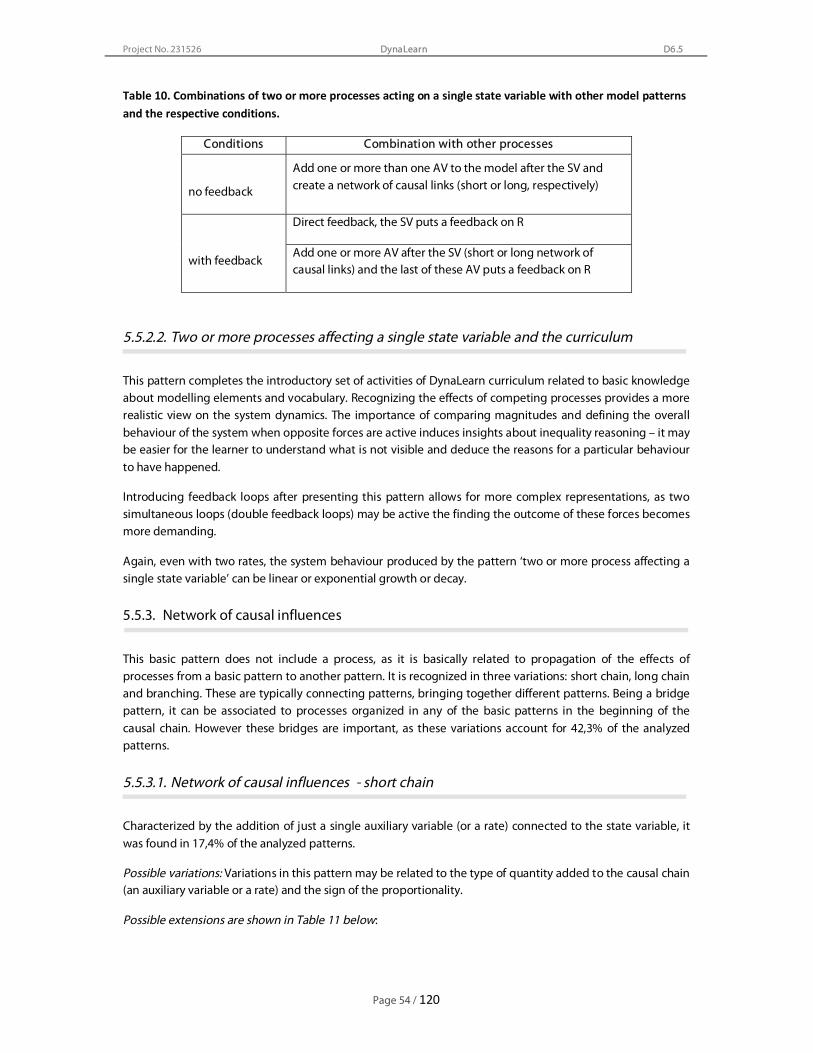
Project No. 231526

/ 120

DynaLearn D6.5

Table 10. Combinations of two or more processes acting on a single state variable with other model patterns and the respective conditions.


no feedback


with feedback



5.5.2.2. Two or more processes affecting a single state variable and the curriculum

This pattern completes the introductory set of activities of DynaLearn curriculum related to basic knowledge about modelling elements and vocabulary. Recognizing the effects of competing processes provides a more realistic view on the system dynamics. The importance of comparing magnitudes and defining the overall behaviour of the system when opposite forces are active induces insights about inequality reasoning – it may be easier for the learner to understand what is not visible and deduce the reasons for a particular behaviour to have happened.

Introducing feedback loops after presenting this pattern allows for more complex representations, as two simultaneous loops (double feedback loops) may be active the finding the outcome of these forces becomes more demanding.

Again, even with two rates, the system behaviour produced by the pattern ‘two or more process affecting a single state variable’ can be linear or exponential growth or decay.

5.5.3. Network of causal influences

This basic pattern does not include a process, as it is basically related to propagation of the effects of processes from a basic pattern to another pattern. It is recognized in three variations: short chain, long chain and branching. These are typically connecting patterns, bringing together different patterns. Being a bridge pattern, it can be associated to processes organized in any of the basic patterns in the beginning of the causal chain. However these bridges are important, as these variations account for 42,3% of the analyzed patterns.

5.5.3.1. Network of causal influences - short chain

Characterized by the addition of just a single auxiliary variable (or a rate) connected to the state variable, it was found in 17,4% of the analyzed patterns.

Possible variations: Variations in this pattern may be related to the type of quantity added to the causal chain (an auxiliary variable or a rate) and the sign of the proportionality.


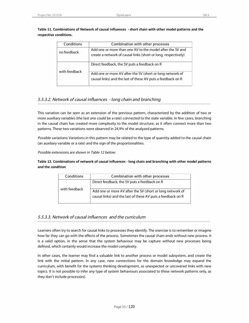
Project No. 231526

/ 120

DynaLearn D6.5

Table 11. Combinations of Network of causal influences - short chain with other model patterns and the respective conditions.


no feedback Add one or more than one AV to the model after the SV and create a network of causal links (short or long, respectively)

with feedback



5.5.3.2. Network of causal influences - long chain and branching

This variation can be seen as an extension of the previous pattern, characterized by the addition of two or more auxiliary variables (the last one could be a rate) connected to the state variable. In few cases, branching in the causal chain has created more complexity to the model structure, as it often connect more than two patterns. These two variations were observed in 24,9% of the analyzed patterns.

Possible variations: Variations in this pattern may be related to the type of quantity added to the causal chain (an auxiliary variable or a rate) and the sign of the proportionalities.


Table 12. Combinations of network of causal influences - long chain and branching with other model patterns and the condition


with feedback



5.5.3.3. Network of causal influences and the curriculum

Learners often try to search for causal links to processes they identify. The exercise is to remember or imagine how far they can go with the effects of the process. Sometimes the causal chain ends without new process. It is a valid option, in the sense that the system behaviour may be capture without new processes being defined, which certainly would increase the model complexity.

In other cases, the learner may find a valuable link to another process or model subsystem, and create the link with the initial pattern. In any case, new connections for the domain knowledge may expand the curriculum, with benefit for the systems thinking development, as unexpected or uncovered links with new topics. It is not possible to infer any type of system behaviours associated to these network patterns only, as they don’t include process(es).

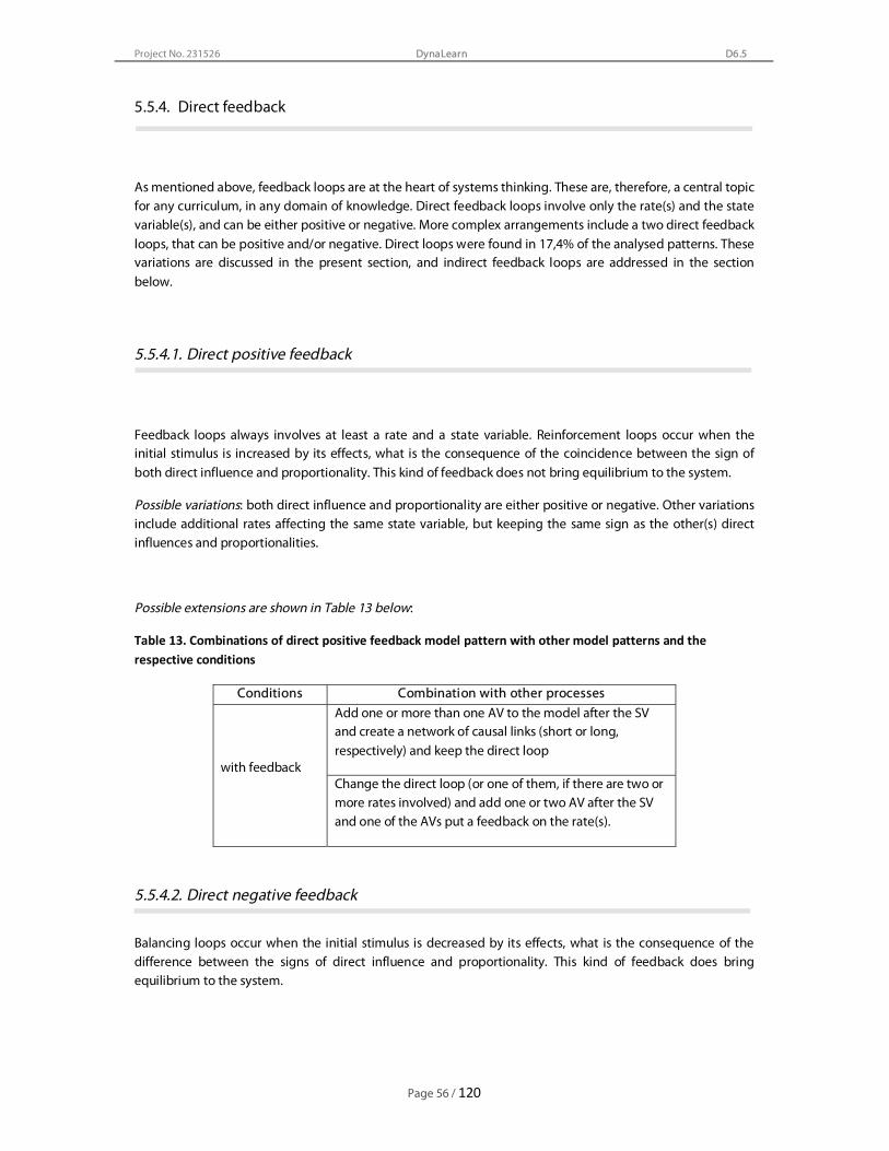
Project No. 231526

/ 120

DynaLearn D6.5

5.5.4. Direct feedback

As mentioned above, feedback loops are at the heart of systems thinking. These are, therefore, a central topic for any curriculum, in any domain of knowledge. Direct feedback loops involve only the rate(s) and the state variable(s), and can be either positive or negative. More complex arrangements include a two direct feedback loops, that can be positive and/or negative. Direct loops were found in 17,4% of the analysed patterns. These variations are discussed in the present section, and indirect feedback loops are addressed in the section below.

5.5.4.1. Direct positive feedback

Feedback loops always involves at least a rate and a state variable. Reinforcement loops occur when the initial stimulus is increased by its effects, what is the consequence of the coincidence between the sign of both direct influence and proportionality. This kind of feedback does not bring equilibrium to the system.

Possible variations: both direct influence and proportionality are either positive or negative. Other variations include additional rates affecting the same state variable, but keeping the same sign as the other(s) direct influences and proportionalities.


Table 13. Combinations of direct positive feedback model pattern with other model patterns and the respective conditions


with feedback

Add one or more than one AV to the model after the SV and create a network of causal links (short or long, respectively) and keep the direct loop

Change the direct loop (or one of them, if there are two or more rates involved) and add one or two AV after the SV and one of the AVs put a feedback on the rate(s).

5.5.4.2. Direct negative feedback

Balancing loops occur when the initial stimulus is decreased by its effects, what is the consequence of the difference between the signs of direct influence and proportionality. This kind of feedback does bring equilibrium to the system.

Project No. 231526

/ 120

DynaLearn D6.5

Possible variations: direct influence can be positive or negative, since the proportionality is negative or positive, respectively. Other variations include additional rates affecting the same state variable, but keeping at least one opposite sign on direct influences and proportionalities.


Table 14. Combinations of direct negative feedback model pattern with other model patterns and the respective conditions.


with feedback

Add one or more than one AV to the model after the SV and create a network of causal links (short or long, respectively) and keep the direct loop

Change the direct loop (or one of them, if there are two or more rates involved) and add one or two AV after the SV and one of the AVs put a feedback on the rate(s).

5.5.4.3. Double direct feedback

Considering that competing (and concordant) processes affecting a single state variable are quite common in natural systems a regular pattern found in DynaLearn models is the one of a double feedback loop. They can be of different types, and it is the reason for different final behaviour of the system. A positive double direct feedback involves two positive single direct loops or two negative single direct loops. The final behaviour is the same, reinforcing the initial stimulus.

A negative double feedback includes one positive and one negative loop. The final behaviour is the result of the negative loop, controlling the initial stimulus. If there are more rates affecting a single state variable, the presence of a negative loop cause to balance to become negative.

5.5.5. Indirect feedback

In ecological and environmental systems, feedback loops may become very complex, and their effects may appear long after the initial stimulus, due to the huge amount of connections between variables. This section deals with indirect feedback loops, model structures that have one or more additional auxiliary variables and one or more of these variables put the influence back on the rate(s).

Variations of this pattern may be classified according the number of additional auxiliary variables in short (one AV) or long chain (two or more AV), and according to the type of feedback (positive or negative). In fact, due to a project decision on limiting the size of the models, only 5,4% of the analysed patterns represent indirect feedback loops, being those with long chains almost 70% of the total in this pattern.

Possible variations: a number of variations are possible when considering short and long chains. Besides the type of dependencies between state variable and auxiliary variable(s),that may be implemented as positive or negative proportionalities, creating many combinations of positive and negative feedback loops, according to the sign of direct influences; and the use of different quantity spaces for the rates, several are the possible variations in the model structure.

Project No. 231526

/ 120

DynaLearn D6.5

Some of them include: feedback loop involving only one of the rates or both; possibility of more than two rates affecting the same SV; possibility of more than one AV being influenced by the SV; possibility of one or more AV influenced by the already existing AV, the first one, which still is the one putting the feedback loop on the rates, expanding the causal chain.

5.5.5.1. Feedback loops and the curriculum

Reasoning about feedback loops is a very relevant topic for learners in the learning by modelling context, as feedback mechanisms are responsible for controlling the system behaviours, and may lead to equilibrium (negative feedback) or complete disequilibrium (positive feedback). It is also possible that, in some models, the feedback loop affects just one of the two rates, or part of the set of influences on the state variable.

Interesting for the curriculum is the opportunity for creating topics or activities in which decisions have to be made. In these cases, the existence of feedback loops may be the chance for the learners to predict the consequences of their actions, and understand how their acts affect their own decisions. Topics for these activities should be polemic, in the sense of having the potential for divide the ‘public’ affected by the decision in two groups – pros and cons.

The system behaviours pattern submitted to these feedback loops, although much more rich and complex, particularly due to negative loops, is still restrict to linear or exponential growth or decay, with the state variables increasing, decreasing and stabilizing.

5.5.6. Inequality reasoning

This is a very productive pattern, as it approaches a quite common situation found in studies about dynamic systems – an unbalanced situation that develops into an equilibrium state. Variations of this pattern may be classified according the number of state variables influenced by the rate, and the number of additional auxiliary variables in in the pattern.

Possible variations: a number of possibilities arise by combining this with other patterns. Initially, the flow, obtained from the calculation between the two auxiliary variables, may have different quantity spaces (zp, mzp); pattern 4 is also a good variation, as may represent multiple influences processes, and movement in opposite directions. For example, the famous (in the QR community) example of the connecting vessels (U-tube) starts with the flow in and flow out set up, and a unique rate (mzp) does the job. Patterns 5 and 6 are also possibilities for propagating the effects on unbalanced situations. Inspiration comes from Patterns 7, 8 and 9.

5.5.6.1. Inequality reasoning and the curriculum

Inequality reasoning feedback loops provide the possibility of expanding the effects of processes to distant parts of the systems, far from where the mechanism of change operates. As a consequence, this kind of feedback may add delays and extra complexity, in which the effects of the loop appear far from the causal origin. These features have potential for including in the curriculum different aspects than those addressed by previous patterns, in which the effects of the processes and feedback loops were direct and the systems represented were relatively simple.

Project No. 231526

/ 120

DynaLearn D6.5

5.6. Examples of using model patterns to build complex models

This section presents three examples of how patterns were combined to produce complex models in DynaLearn.

5.6.1. Combining single rate/ process + network + direct feedback

The model “Urbanization affects fish community”, by IBER (D6.4.3, Borisova et al. 2011) exhibits a low level of complexty, and combines the following basic patterns: ‘single process/ single rate’, network of causal relations – short chain’ and ‘direct feedback’, as shown in the Figure 21:

Figure 21. Part of the model “Urbanization affects fish community”, showing a sequence of patterns: single processes affect short chains of causality, ending in a single positive direct feedback.

The analysis of the model shows how the basic patterns can be repeated to produce a longer causal chain that ends in a direct feedback:

- Basic pattern ‘single process/ single rate’ involving the quantities Entity Urban population Urbanization (rate) and Size;

- Basic process ‘network of causal relations – short chain’ involving the quantities Entity Urban population Size and Sewage production;

- Basic pattern ‘single process/ single rate’ involving the quantities Entity Urban population Sewage production (rate) and Entity Wetlands Nutrients;

- Basic process ‘network of causal relations – short chain’ involving the quantities Entity Wetlands Nutrients and Entity Algae community Growth;

- Basic process ‘direct feedback’ involving the quantities Entity Algae community Growth (rate) and Biomass.

Project No. 231526

/ 120

DynaLearn D6.5

5.6.2. Combining inequality reasoning + network + indirect feedback

This section presents the Model ‘Lotka Volterra advanced A’ by BOKU ( D6.4.5, Zitek et al. 2011) which causal model is shown in Figure 22. The model results from the combination of two instances of ‘inequality reasoning’ via two instances of ‘network of causal relations – short chain’, creating an ‘indirect feedback loop’. Being a negative loop involving two state variables, the model produces the delayed oscillation behaviour typically expected for the predation-prey system (see Principle 5 in section 6.2.5; and section 5.2.1 for the combination of patterns).

Figure 22. Model ‘Lotka Volterra advanced’, based in two representations of the basic patterns ‘inequality reasoning’ and ‘network – short chain’.

- Basic ´pattern ‘inequality reasoning pattern’, applied twice, with the Entities Rabbit and Fox; the Entity population has four quantities and the value of the rate Population growth rate is calculated using the arithmetic operation of subtraction as follows:

Population growth rate = Number of births ( – ] Number of deaths

and the rate further influences the state variable Population size.

- Basic process ‘network of causal relations – short chain’ also repeated twice, involving the quantities Entity Rabbit population Population size.and Entity Fox population Number of births; and Entity Fox population Population size.and Entity Rabbit population Number of deaths.

Project No. 231526

/ 120

DynaLearn D6.5

5.6.3. Combining single rate/ multiple process + inequality reasoning etc.

The Model ‘Cellular osmosis and diffusion’ by UH (D6.4.2, Noble and Cowx, 2011) presents a high level of complexity and involves exogenous variables and ‘single process/ multiple influences’, ‘inequality reasoning’, ‘network of causality – long chain’ and ‘indirect feedback – long chain’ patterns, as shown in the Figure 23.

Figure 23. Model ‘Cellular osmosis and diffusion’ by UH (Noble and Cowx, 2011) showing a combination of Patterns ‘single process/ multiple influences’, ‘inequality reasoning’, ‘network of causality – long chain’ and ‘indirect feedback – long chain’ .

The patterns identified in this model causal are the following:

- Simulation starts with two exogenous quantities: Entity internal solute, Amount; Entity external solute, Amount;

- Basic pattern ‘single process/ multiple influences’, involving Entity Membrane, rates Osmosis in and Osmosis out;

- Variation of ‘inequality reasoning pattern’, in which Entity Membrane has two quantities Concentration gradient and Water potential gradient both calculated using the arithmetic operation of subtraction but they do not put influences on other quantities as follows:

Concentration gradient = Entity Internal solution Concentration ( – ] Entity external solution Concentration

Water potential gradient = Entity External solution Water potential ( – ] Entity Internal solution Water potential

Project No. 231526

/ 120

DynaLearn D6.5

- Basic pattern ‘network of causality – long chain’ involving, for example, the quantities Entity External solvent Volume Æ Entity External solution Concentration Æ Entity Membrane Concentration gradient;

- Basic pattern ‘indirect feedback – long chain’, involving, for example, the following quantities: Entity Membrane Osmosis out Æ Entity Internal solvent Volume Æ Entity Internal solution Concentration Æ Entity Internal solution Water potential Æ Entity Membrane Osmosis out.

5.7. Discussion

Basic skills related to systems thinking and the key points to have in mind while building qualitative system dynamics models were discussed in this section. Based on these elements, ideas about what are the ultimate goals of DynaLearn curriculum and learning activities (the development of cognitive, reasoning and systems thinking skills) and the toolbox represented by generic model structures form the basis for model progression.

Model progression in qualitative system dynamics could go through the following guidelines:

• Always associate the selected model pattern to the behaviour it produces; • Try to find out examples of real systems to which the patterns are applicable; • Start simple and scale up to complexity by combining patterns; • Create the model step by step, following a compositional modelling approach.

The following section discuss good modelling practices in DynaLearn, taking into account the facilities provided by semantic technology, virtual characters and the whole set of Learning Spaces, particularly LS4, 5 and 6.

Project No. 231526

/ 120

DynaLearn D6.5

6. Good modelling practices

6.1. Background

Learning by modelling has been put forward as a rich and effective means of learning which fosters both development of domain knowledge and the cognitive reasoning skills of the learner. As such, modelling becomes a powerful tool for students for both expressing ideas and for evaluating and integrating new information. Modelling also develops a constructivist approach to learning where learners can construct and test their own knowledge about the world around them. This approach is fundamental in science education for developing students understanding of scientific method and scientific reasoning skills. Within this, good practice needs to be developed, both in terms of building models for educational purposes and for the modelling process itself, to facilitate the implementation of learning by modelling with DynaLearn within education curricula.

Learning by modelling can be viewed as a process through which students develop a new or deeper understanding of a domain system they are studying. So whilst a goal of a learning exercise might be for the student to create a model that represent current expert theories and understanding the process of building the model itself can be viewed as important. The DynaLearn modelling approach explores the idea of mental models ((Gentner and Stevens, 1983; see also Appendix G). By facilitating the externalisation of mental models into conceptual models using a formal representation that can be tested through simulation and comparison with expert representations and model patterns, DynaLearn develops structured modelling and reasoning skills for the student that enables them to build better models and internal representations of the domain.

Following this approach it can be recognised that good modelling practice in an educational context has two key domains: (1) Good modelling practice in terms of the modelling process; and (2) Good modelling practice in terms of the qualities of expert/teacher models used as references or targets for learning. This section explores good modelling practice in the context of the potential requirements of expert/teacher reference models, the learning by modelling process (student model perspectives) and the influence of the technological aspects of the DynaLearn system on modelling practice.

6.2. Good modelling practice as a learning activity

6.2.1. Learning by modelling approaches

The modelling process can be seen to have five main stages in relation to model development and learning. These stages are: (1) creation of a mental model of the system based on the learners existing knowledge, new stimulus didactic materials and some sort of problem or question for the model to answer; (2) the externalisation and formalisation of the internal view of the system into a conceptual model that can be communicated; (3) testing of the efficacy of the conceptual model through simulation and/or comparison with reference models (both components of the DynaLearn system); (4) re-evaluation and development of the conceptual model; and (5) internalisation of knew knowledge into the students’ mental model of the system. Learning by modelling approaches therefore needs to support all five of these stages.

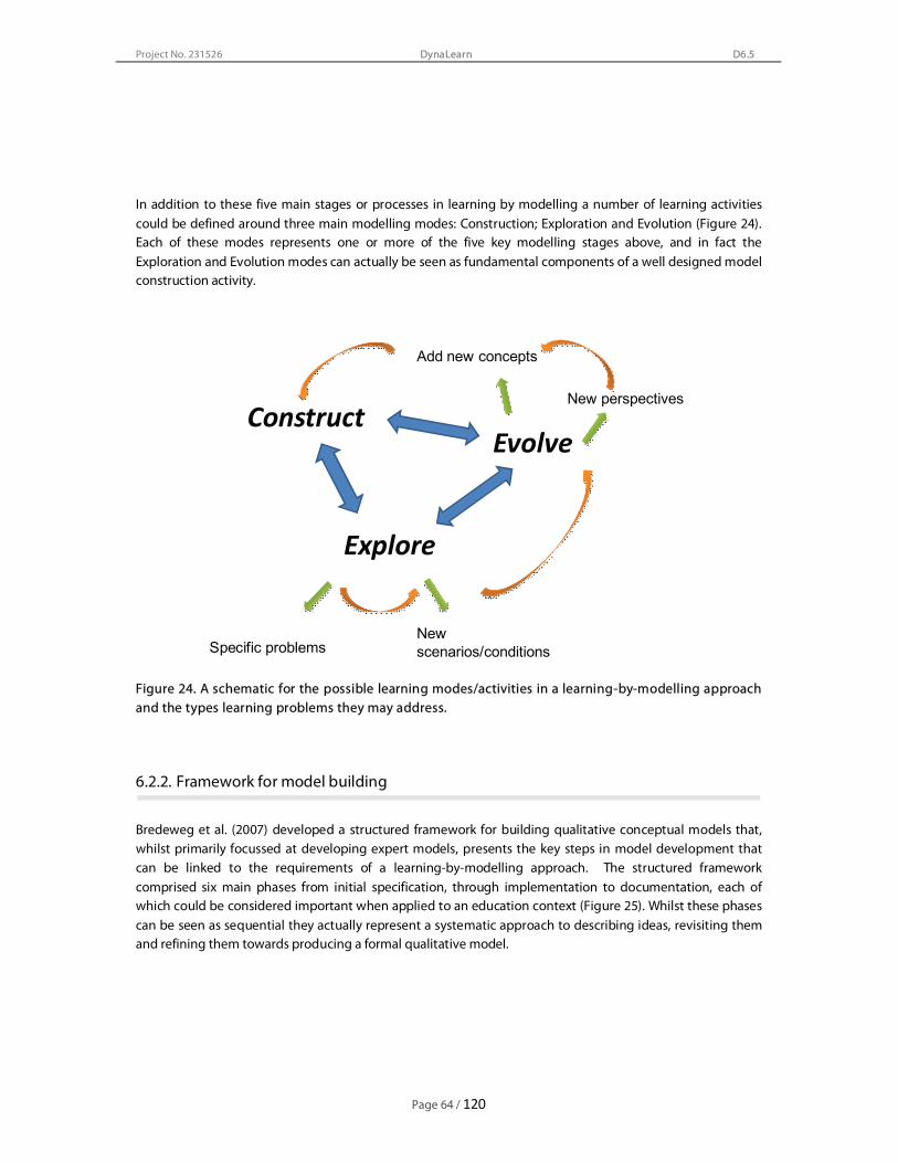
Project No. 231526

/ 120

DynaLearn D6.5

In addition to these five main stages or processes in learning by modelling a number of learning activities could be defined around three main modelling modes: Construction; Exploration and Evolution (Figure 24). Each of these modes represents one or more of the five key modelling stages above, and in fact the Exploration and Evolution modes can actually be seen as fundamental components of a well designed model construction activity.

Construct

Explore

Evolve

Add new concepts

New perspectives

New scenarios/conditionsSpecific problems

Figure 24. A schematic for the possible learning modes/activities in a learning-by-modelling approach and the types learning problems they may address.

6.2.2. Framework for model building

Bredeweg et al. (2007) developed a structured framework for building qualitative conceptual models that, whilst primarily focussed at developing expert models, presents the key steps in model development that can be linked to the requirements of a learning-by-modelling approach. The structured framework comprised six main phases from initial specification, through implementation to documentation, each of which could be considered important when applied to an education context (Figure 25). Whilst these phases can be seen as sequential they actually represent a systematic approach to describing ideas, revisiting them and refining them towards producing a formal qualitative model.

Project No. 231526

/ 120

DynaLearn D6.5

Figure 25. The model building framework and sequence of modelling activities/intermediate model products proposed by Bredeweg et al. (2007).

Of the six stages proposed by Bredeweg et al. (2007) four of them can be seen as the basis for learning by modelling: (1) Orientation and initial specification of the model; (2) System selection and global behaviour; (3) Detailed system structure and behaviour; and (4) Implementation (including simulation and testing). These four stages can be viewed alongside the five stages of learning by modelling described above. Essentially these relate to: (1) the stimulus for modelling (either teacher of learner specified) and the situated perspective of the modelling exercise; (2) the externalisation of the students mental model of the problem/system using their current understanding and vocabulary; (3) the formalisation of the students mental model from their own vocabulary into a structured modelling approach or vocabulary; and (4) the implementation, testing and adjustment of a structured conceptual model in a formal modelling tool. Bredeweg et al. (2007) proposed that the first three of these stages could be done outside of the specific modelling software and they would produce important explicit representations of intermediate results. However, for an optimal learning-by-modelling approach it would be beneficial for the key stage in modelling, the transition from the mental model to the formalised conceptual model, to occur within a single modelling environment that facilitated this modelling transition and provided individualised feedback and support during this process. Therefore, any learning-by-modelling activity undertaken within DynaLearn needs to be designed taking into account the requirements to facilitate the transition from mental model to formalised model and this also needs to consider the difference between naive modellers (those with no experience of the QR vocabulary or systems viewpoint) and experienced modellers.

Therefore, the design of self-directed learning activities (Gibbons 2002; Carneiro et al. 2011) within DynaLearn and the definition of a curriculum for learning by modelling needs to consider the following elements:

• long-term modelling curricula

o the needs and abilities of student modellers

o the support needed to learn the representation vocabulary and approach

Project No. 231526

/ 120

DynaLearn D6.5

• Activity/Topic specific curricula

o the likely properties of naive student models;

o the required properties of expert models used as references (representing both accurate domain material and potential good practice in QR representations)

o The mode of working and how this is facilitated by the software.

In general this translates into a new framework for learning by modelling, particularly with reference to a curricula perspective and supporting learning activities. This can be represented on two axes (1) learning by modelling processes and (2) learning goals and skills.

1. Learning by modelling processes

a. Stimulus & Goal setting

b. Externalisation of a mental model (in the case formalisation in DL)

c. Refinement of a model by comparison with other models (Recommendation)

d. Refinement of a model by testing it with simulation (Simulation, Why? And Diagnosis)

e. Reflection and internalisation of new knowledge (resulting from b-d)

2. Learning goals and skills

a. Domain knowledge

b. Learning QR vocabulary and representations

c. Development of a systems viewpoint (systems thinking)

d. Developing scientific reasoning skills

6.3. Good modelling practice in reference models

6.3.1. Aspects of good modelling practice identified in D6.3

The review of the basic topics and models delivered in D6.2.(1-5) undertaken within D6.3 identified two main areas in QR representation where good modelling practice needed to be evaluation. These were (1) representation of system structure and the definition or entities and quantities (plus use of configurations); and (2) the use and definition of quantity spaces within a model. These two areas of modelling practice were linked to both fundamental approaches in QR representation and to the technological and pedagogical aspects of their utility in the DynaLearn software. This generally represented the aspects of (1) complexity in models and simulations resulting from QS definitions; and (2) nomenclature of ingredients and the role that played in the implementation of grounding and recommendation, and the vocalisations of the virtual characters. This section revisits and refines these ideas in the light of the results of the advanced modelling activities from D6.4.(1-5), model patterns and the advances in the DynaLearn software.

Project No. 231526

/ 120

DynaLearn D6.5

6.3.2. Advanced models and expert modelling practices

Following the internal review of basic topics and models, Deliverable D6.3 (Noble et al. 2011) identified that advanced models should be focussed around the most important patterns and processes within curricula topics. Furthermore, the advanced models should be insightful and situated at an appropriate level of complexity to capture insightful explanations of phenomena, taking best advantage of the available features of each Learning Space in DynaLearn.

The features identified for “advanced models” in D6.3 included a number of features that can be linked to good modelling practice for expert/reference models:

• Models representing more complex phenomena by integration of basic laws and first principles to address a more complex problem;

• describe mechanisms that explain how things work and integrate;

• develop formal explanations for the system behaviour of advanced topics;

• advanced models should be optimised to exploit the software capabilities.

The models delivered as part of D6.4.(1-5) therefore focussed on:

• being clearly and suitable framed within a domain topic and having an appropriate curricula context.

• making appropriate use of different Learning Spaces to convey explanations for conceptual ideas.

• optimising their use by the technological components of DynaLearn.

• having consistency in their design and the approach to nomenclature from an expert, technological and educational perspective.

• Showcasing the opportunities and technologies created by the DynaLearn environment.

Despite having more clearly focussed goals and a more consistent approach this formalising of modelling practices still enabled modellers to produce diverse models in terms of content and style. This flexibility, even within a structured approach, is a strength when considering the diversity of topics and concepts that can be handled in an environmental science curriculum. Fundamentally, the single most important aspect of good modelling practice for the process of building reference models was to clearly and suitably frame the model within a domain topic, clearly specifying from a stimulus text or diagram the fundamental system behaviour/phenomenon they should represent. Having a clearly specified behaviour (for example density-dependent population growth and the sigmoid growth curve, or the Lotka-Volterra model) focussed model building and tended to result in models that presented formal explanations for complex phenomena that integrated information from basic laws and first principles. Furthermore, work in T6.4 on advanced models lead to a further refinement of approaches with QR representations. Of great relevance for this discussion is the possibility of using model patterns to express subsystems’ behaviour and to find some hints on how to progress in the model building implementing modelling solutions provided by the combination of model patterns (see Section 5.5).

Project No. 231526

/ 120

DynaLearn D6.5

6.3.3. Advancement of representations - good modelling practice

In terms of representations in QR development of good modelling practices relate to the nomenclature and approach used for defining system structure and the use and definition of quantity spaces in models to control or represent behaviours. The result of advanced modelling in D6.4. (1-5) highlighted some approaches to this.

A) Model system structure

Essentially this aspect of good practice relates to the definition and use of entities and quantities in models to define the system structure. This is important as this is one step in modelling that is found to be initially difficult by novice learners. As a result of this it is important that the use of entities and quantities follow a consistent approach such that their definitions and use can be easily learnt. There were two main views on how this could be handled consistently.

Hierarchically Entities Objects in the system at the scale considered

Quantities Aspects of those entities that could be measured/change

Physically Entities All physical aspects of the system regardless of scale

Quantities Dimensions such as weight, height, amount etc.

These two approaches differ primarily on the use of scale and granularity in models, the strict physical option has set definitions of an entity and quantity whereas the hierarchical option enables models to be potentially more concise in representations. For example, a model focussing on a scale where a Forest could be an important entity could be represented in two different ways:

Hierarchically Entities Forest

Quantities Number of trees

Physically Entities Forest AND Trees

Quantities Number of

In reality both systems are valid and probably interchangeable as both present a consistent approach to nomenclature. The hierarchical approach is preferred from a conceptual viewpoint as it promotes concepts of system hierarchy and also handles complexity and scale issues. The physical viewpoint has benefits in terms of relative simplicity (all physical objects are entities and quantities are merely dimensions) however it would have a tendency to result in complex and cluttered model expressions with lots of entities many of which would not have associated quantities (and as such would have no influence on the system behaviour). However, it should be noted that the choice of approach, at least initially as the software and repository of models are developed, has significant implications for grounding and recommendation technologies.

B) Quantity spaces and qualitative states

Noble et al. (2011) identified that a parsimonious approach should be applied to the definition of quantity spaces, where the spaces are only expanded where there is a need to show explicitly distinct qualitative states or there is a clear need to visualise behaviour within a simulation value history. This approach was used for many models delivered in D6.4 and played a fundamental role in the ability to create clear and simple representations of key behaviours.

Project No. 231526

/ 120

DynaLearn D6.5

For a more complete discussion about the creation of quantity spaces and key questions to be answered while deciding for inclusion of points and intervals, see Appendix D.

6.3.4. Good modelling practice – links to grounding and recommendation

Noble et al. (2011) identified that good modelling practice for expert representations had close links to the technological requirements of the DynaLearn system from the point of view of the verbalisation of model components by the virtual characters and the handling and automated matching of model ingredients by the semantic technology. Whilst it is possible to define what should be done for expert models and by the technological components themselves to optimise this expert model-technology interaction it is impossible to define how this relates to the naive model-technology interaction. Although, verbalisation of models by characters is important for high quality virtual character mediated model interactions these interactions tend to be focused on expert models (e.g. TA mode, Quiz) and as such can be addressed in the model development and the scripting technology. Therefore, the grounding-recommendation technology/student mode interaction is of greatest importance here. The grounding process and ontology matching technology is the fundamental tool to allow students to improve their model in terms of nomenclature, complexity and causal representation. However, this requires that the tool can identify the content of a student model and match it to an appropriate reference model or suite of reference models. This relies fundamentally on identifying models with elements with similar groundings. Given this, the choice of approach to entity/quantity definition will have large implications for the performance of model matching.

Hierarchical Compound terms such as “Number of trees” are not be present in DBpedia and require creation of anchor terms. This could result in a large number of different anchor terms being created for similar concepts – or potentially each individual student creating an anchor term to match their own initial nomenclature. This could result in the semantic technology not being able to find any overlapping reference models to provide recommendations to the student. It is unlikely in this system that matches based purely on grounding overlaps could link models which had “Trees” as entities to this student model.

Physical/Strict In this approach the strict definition of entities and quantities would mean that once groundings were available for “Forest”, “Trees” and for the dimension “Number of” then all new modellers would be much more likely to use pre-existing definitions from the repository. Such an approach would make it much more likely for students to obtain relevant feedback on models matched through common groundings alone. This system would also allow for the system to match other models where “Trees” were the main focus as an entity.

Given this, whilst hierarchical approach to entity and quantity definition from a modelling point of view, it should be noted that the hierarchical approach would undoubtedly have implications for the early performance and capability of the ontology-based feedback and recommendation system. In fact it is probable that the interaction between nomenclature and grounding will have the single biggest influence on the performance of the DynaLearn system and its support of self-directed modelling. However, given the current formulation of how learners interact with the reference models this aspect is actually beyond the control of the reference models and needs to be address by the wider learning by modelling curricula and the implementation of the technology.

Project No. 231526

/ 120

DynaLearn D6.5

6.4. Integration of good modelling practice and learning spaces

Integration of the good modelling practices discussed above and the actual activities of building models in DynaLearn can be facilitated with the support of the set of model patterns. In this section the development of a model exploring an environmental issue is discussed. Initially, a LS4 is created. Next, conditional knowledge is implemented in LS5, and finally guidelines for the implementation of a LS6 version of the model.

6.4.1. Modelling in Learning Space 4

6.4.1.1. From text to model

During the modelling process reference texts are good instruments to support the modeller, especially in the phase when the objects of the system and the nature of relationships between them need to be determined. Reading a text it’s possible to identify entities, quantities and processes and express them in the model, more details were approached in section 5.2.1 and the complete exercise can be found in the Appendix E.

6.4.1.2. Hydrological Erosion model In Learning Space 4

Figure 26 show a model built in LS4 about hydrological erosion.

Figure 26. Hydrological Erosion LS4 model.

Pattern: single rate/process

Two rates/processes affecting a single state variable

Project No. 231526

/ 120

DynaLearn D6.5


Conditional knowledge is an important information to represent correctly the behaviour of many systems. The Figure 27 demonstrates a conditional knowledge represented in a model using the Learning Space 5 of the DynaLearn.

Figure 27. Algae Bloom LS5 conditional fragment. This Conditional Expression Fragment can be represented in one fragment in Learning Space 6. Top: Expression conditional fragment 2a: if Toxins has value equal or greater than critical, then there is a negative proportionality from Toxins to Number of (Fishes). Bottom: expression conditional fragment 2b is the opposit situation, that is, if Toxins has value lower than critical, then the Number of (Fishes) is constant it must be represented in another conditional expression fragment.

Project No. 231526

/ 120

DynaLearn D6.5


There is an important consideration: the way patterns are represented depends on the definitions and the modelling choices made by the modeller to consider basic patterns instead of combined ones when it is the case. Here the modeller can chose to consider erosion and formation rates as a single patterns and place them in the same model fragment or can place them in different model fragments Figure 28. The complete exercise can be found in the Appendix E.

Figure 28. Water Erosion LS4, demonstrating how to recognize patterns in the model as a important step for represent it in the Learning Space 6.

6.5. Discussion

Having explored possible routes for model progression in section 5, time has come to introduce the elements that support modelling decisions. Considering what has been identified as good modelling practices meta-level analyses of the topic of interest should be considered to drive the selection of model patterns and refinements of the knowledge to be captured by the model. Adaptations in a framework for building qualitative models are proposed, so that well designed model building activities integrate construction, exploration and evolution in a learning by modelling context. Facilities provided by DynaLearn, such as grounding and recommendation, support the implantation of good modelling practices.

1 – It is possible to represent each process in separate model fragments

2 – It is possible to represent the effects of processes in other model fragments 3 – It is possible to represent other

effects and their propagations in separate model fragments

Project No. 231526

/ 120

DynaLearn D6.5

Taking the ‘Hydrological erosion’ model as example, the main steps of a learning by modelling approach dedicated to the development of systems thinking are presented (Appendix E). Firstly, the learner is stimulated to abstract from a text key modelling elements necessary to create a LS4 model. It is time to identify processes, entities, quantities and quantity spaces, propagation of changes in the system, conditional knowledge needed to assess the effects of processes. In doing so, the learner shall develop systems thinking skills (section 5.1) as dynamic thinking (deduce behaviour patterns), generic thinking (generate specific occurrences in different domains – vegetation, soil, energy production, economy), structural thinking (distinguish between rates and state variables) and operational thinking (to capture how things interact in a complex mechanism).

Following the stages proposed in section 6.2.2 for the framework for model building and model patterns available in the toolbox, the learner produces a LS 4 model (section 6.4.1). Adding conditional knowledge, creates a LS 5 model. And having the set of model patterns as first choice, move to a more compact, hierarchical and reusable version of the ‘Hydrological erosion” LS 6 model.

Very important is to take into account additional material to contextualize the modelling effort, a set of cognitive and reasoning skills, exercises to use DynaLearn functionalities, evaluation materials. These aspects were not mentioned in the space available for this deliverable, but cannot be underestimated.

This way, a complete cycle of DynaLearn curriculum has been accomplished.

Project No. 231526

/ 120

DynaLearn D6.5

7. Conclusions

The tentative of putting into practice an educational proposal compiled in this document as DynaLearn curriculum for environmental science is based on the results of WP6 and takes into account the evaluation studies in WP7.

Following the main aspects related to curricula, as put by Stenhouse (1975), the conclusions of the present work can be summarized as follows.

DynaLearn curriculum offers as planning principles to select the contents to be learned the notion of priority to fundamental knowledge, laws, principles in environmental science and mechanisms able to explain how ecological systems operate and relate to current trends and environmental phenomena. Most of the themes and topics selected in Task 6.1 have proven to be adequate, and the advanced models produced by the project shed some light on how to address these topics.

Applications to different domains are for sure possible. The basis of DynaLearn curriculum (learning by modelling, based in model patterns and focussing on systems thinking and cognitive skills) fits well to topics in almost all disciplines.

Decisions about the sequence of contents to be addressed are left for those responsible for the educational activities based in this curriculum. In fact, DynaLearn curriculum contents are seem as a web of topics, to be explored in accordance to local needs and interests.

The pedagogical strategy is based on learning by modelling approaches. It is assumed that learners that master the modelling language and the software are able to self-direct their own learning processes, at least with respect to the disciplines that can be addressed by modelling. However, there is a lateral issue to be explored in DynaLearn curriculum, the one that refers to learning how to model. Key points on qualitative system dynamics, model patterns and good modelling practices provide the handles for the learners to get autonomy in modelling issues.

Model patterns are a relevant part of DynaLearn curriculum. Both for the learners and for the teachers, these generic pieces of model structures have the potential for making the learning process less demanding. A curriculum based on which sequence to follow while presenting the patterns is part of ongoing work. Investigations and empirical studies about the tendency observed in this work, about a positive correlation between modelling experience and preference for more complex patterns are still to be confirmed.

Mechanisms to measure progress of learners and teachers in using a qualitative system dynamics approach and DynaLearn software exist, as products of this project. However there is room for their improvement. This is part of ongoing work.

Feasibility of implementing DynaLearn curriculum in pre-college schools is high, but at university is higher. Provide there is time available for using the modelling workbench in the classroom, and the adherence of the teachers to the proposal of adopting systems thinking as a goal to be achieved. However, much has to be changed in current school organization, curricula, and the way teaching is done.

Project No. 231526

/ 120

DynaLearn D6.5

References

Stanley, L. (1996). Graphical Integration Exercises Part 4: Reverse Graphical Integration (D-4603), System Dynamics in Education Project, System Dynamics Group, Sloan School of Management, Massachusetts Institute of Technology, August 20, 24 pp.

Ashford, A.C. (1995) Unexpected Behaviours in Higher-Order Positive Feedback Loops. Paper available for download at <http://ocw.mit.edu/courses/sloan-school-of-management/15-988-system-dynamics-self-study-fall-1998-spring-1999/readings/unexpected.pdf>. Access in May, 2012.

Borisova, P. and Uzunov, Y. (2011). CLGE advanced topics and models. DynaLearn, EC FP7 STREP project 231526, Deliverable D6.4.3.

Borisova, P., Nakova, E., & Uzunov Y. (2010). Central Laboratory of General Ecology – Basic topics and models DynaLearn, EC FP7 STREP project 231526, Deliverable D6.2.3.

Bredeweg, B. and Salles, P. (2009). Qualitative models of ecological systems – editorial introduction. Ecological Informatics, 4(5-6), 261–262.

Bredeweg, B. and Struss, P. (2003). Current Topics in Qualitative Reasoning. AI Magazine, 24(4), 13-16.

Bredeweg, B., Liem, J., Beek, W., Salles, P. and Linnebank, F. (2010). Learning Spaces as Representational Scaffolds for Learning Conceptual Knowledge of System Behaviour. In Wolpers, M., Kirschner, P.A., Scheffel, M., Lindstaedt, S. and Dimitrova, V. (eds.), Sustaining TEL: From Innovation to Learning and Practice (EC-TEL 2010), p47-61, LNCS 6383, Barcelona, Spain.

Bredeweg, B., Linnebank, F., Bouwer, A. and Liem, J. (2009). Garp3 – Workbench for Qualitative Modelling and Simulation. Ecological Informatics 4(5-6), 263-281.

Bredeweg, B., Salles, P., Nuttle, T. (2007). Using exogenous quantities in qualitative models about environmental sustainability. AI Communications, 20(1), 49-58.

Carneiro, R.; Lefrere, P.; Steffens, K.; and Underwood, J. (eds.) (2011) Self-Regulated Learning in Technology Enhanced Learning Environments: A European Perspective. Roterdam, Sense Publishers.

Caulfield, C. W., and Maj, S. P. (2001). "A Case for Systems Thinking and System Dynamics." Proceedings of the IEEE International Conference on Systems, Man and Cybernetics, Tucson, AZ, 2793 - 2798.

Chung, C. 1994. Generic Structures in Oscillating Systems I (D-4426-1), System Dynamics in Education Project, System Dynamics Group, Sloan School of Management, Massachusetts Institute of Technology, June 17, 24 pp. Paper available at <http://clexchange.org/ftp/documents/Roadmaps/RM6/D-4426-3.pdf>. Access in May, 2012.

Correa, A.C. (2011) Modelos Qualitativos de Simulação sobre a Dinâmica do Plâncton em Diferentes Estados de Trofia no Lago Paranoá, DF. MSc dissertation, Graduate Program in Ecology, University of Brasília, Brazil (in Portuguese).

De Kleer, J. and Brown, J.S. (1981) Mental models of physical mechanisms and their acquisition, in: J.R. Anderson (Ed.), Cognitive Skills and their Acquistion. Erlbaum, Hillsdale, NJ, 1981, 285-309

Project No. 231526

/ 120

DynaLearn D6.5

Dodds, W.K. (2009) Laws, theories and patterns in Ecology. Berkeley-Los Angeles, University of California Press.

Elsom-Cook, M. (2001). Principles of interactive multimedia, 350 pages, McGraw-Hill.

Ernest, A.W. (1975). Subjunctive and indicative conditionals. Foundations of Language, 6(1), 89–94.

Eurydice (2006). Science Teaching in Schools in Europe Policies and Research. Eurydice, the information network on education in Europe (http://www.eurydice.org).

Falkenhainer, B. and Forbus, K. (1991). Compositional Modelling: Finding the Right Model for the Job. Artificial Intelligence, 51(1 3): 95 143.

Forbus, K.D. (1984). Qualitative process theory. Artificial Intelligence, 24, pp. 85-168.

Forrester (2009) Learning through System Dynamics as Preparation for the 21st Century. paper, revised version (2009) available at <http://clexchange.org/ftp/documents/whyk12sd/Y_2009-02LearningThroughSD.pdf>. Access in May, 2012.

Forrester, J. (1997) System Dynamics and K-12 Teachers. A lecture at the University of Virginia School of Education, USA, May 30, 1996. Paper available for download at <http://ocw.mit.edu/courses/sloan-school-of-management/15-988-system-dynamics-self-study-fall-1998-spring-1999/readings/teachers.pdf>. Access in April, 2012.

Forrester, J.W. (1971) Counterintuitive Behaviour of Social Systems. Available at <http://ocw.mit.edu/courses/sloan-school-of-management/15-988-system-dynamics-self-study-fall-1998-spring-1999/readings/behaviour.pdf> Accessed in April 2011.

Gibbons, M. (2002). The self-directed learning handbook. San Francisco, CA: Jossey-Bass

Gotelli, N.J. (1995) A Primer of Ecology. Sunderland, MA, Sinauer Associates.

Gentner, D. and Stevens, A.L. (1983). Mental models. Hillsdale, NJ, Lawrence Erlbaum Ass. Inc.

Haefner, J.W. (2005) Modelling Biological Systems: Principles and Applications. 2nd. ed. New York, NY: Springer Science+Business Media, Inc.

Iwasaki, Y. and Simon, H.A. (1986). Causality in device behaviour. Artificial Intelligence, 29(1), 3–32.

Kleer, de J. and Brown, J.S. (1984). A qualitative physics based on confluences. Artificial Intelligence, 24, 7–83.

Kuipers, B. (1994). Qualitative Reasoning: Modelling and Simulation with Incomplete Knowledge, 452 pages, MIT Press.

Leiba, M., Zurel, D., Mioduser, D., and Benayahu, Y. (2011). TAU Advanced models and topics. EC FP7 STREP project 231526, Deliverable D6.4.4.

Liem, J., Beek, W. and Bredeweg, B. (2010a). Multi use level workbench. DynaLearn, EC FP7 STREP project 231526, Deliverable D3.1.

Liem, J., Beek, W. and Bredeweg, B. (2010b). Differentiating Qualitative Representations into Learning Spaces. 24th International Workshop on Qualitative Reasoning (QR’10). de Kleer, J. and Forbus, K.D. (eds.), pages 37-46, Portland, Oregon, USA, 8-10 August 2010.

Project No. 231526

/ 120

DynaLearn D6.5

Martin, L. A. (1997). An introduction to feedback. paper available at http://ocw.mit.edu/courses/sloan-school-of-management/15-988-system-dynamics-self-study-fall-1998-spring-1999/readings/feedback.pdf. Access in April, 2012

Mioduser, D., Zuzovsky, R. (eds.), Salles, P., Souza, A., Portella, A., Braga, E., Wilhelms, L., Pereira Resende, M., Morison, G., Assumpção da Costa e Silva, P., Gontijo de Sá, I., Pires, L., Simões, A., Noble, R., Borisova, P., Uzunov, Y., Zurel, D., Leiba, M., Benayahu, H., Nachmias, R., Ram, J., Zitek, A., Poppe, M., & Stelzhammer, M. (2011). Evaluation of DynaLearn – first phase insights. DynaLearn, EC FP7 STREP project 231526, Deliverable D7.2.6.

Mioduser, D., Zuzovsky, R., Salles, P., Souza, A., Portella, A., Braga, E., Wilhelms, L., Pereira Resende, M., Morison, G., Assumpção da Costa e Silva, P., Gontijo de Sá, I., Pires, L., Simões, A., Noble, R., Cowx, I., Borisova, P., Liem, J., Uzunov, Y., Zurel, D., Leiba, M., Benayahu, H., Nachmias, R., Ram J., Zitek, A., Poppe, M. & Stelzhammer, M. (2012). Final report on DynaLearn evaluation studies. DynaLearn, EC FP7 STREP project 231526, Deliverable D7.4.

Mioduser, D., Zuzovsky, R., Zurel, D., Leiba, M., Benayahu, Y., Nachmias, R., & Ram, J. (2010). TAU evaluation of DynaLearn prototype. DynaLearn, EC FP7 STREP project 231526, Deliverable D7.2.4.

Noble, R. (2010). University of Hull – Basic Topics and Models. DynaLearn, EC FP7 STREP project 231526, Deliverable D6.2.2.

Noble, R. and Cowx, I. (2011). UH – Advanced topics and models. DynaLearn, EC FP7 STREP project 231526, Deliverable D6.4.2.

Noble, R., Salles, P., Zitek, A., Mioduser, D., Zuzovsky, R. and Borisova, P. (2011). DynaLearn curriculum reflection and advancement. DynaLearn, EC FP7 STREP project 231526, Deliverable D6.3.

Odum, E.P. (1985). Ecologia. Rio de Janeiro: Discos CBS. (Translation into Portuguese of Basic Ecology)

Pearl, J. (2009). Causality: Models, Reasoning and Inference, 484 pages, Cambridge University Press.

Pickett, S.T.A.; Kolasa, J.; Jones, C.G.( 2007). Ecological understanding: the nature of theory and the theory of nature. 2nd edition. Academic Press, London, 2007.

Pinker, S. (2007). The Stuff of Thought: Language as a Window into Human Nature, 512 pages, Viking Penguin.

Richmond, B. (2001). An introduction to systems thinking, STELLA. Hanover, NH, High Performance Systems Inc.

Richmond, B. (1993). Systems thinking: critical thinking skills for the 1990s and beyond. System Dynamics Review, 9(2), 113-133.

Road Maps Glossary, (2005). Road Maps Glossary. Available at <http://clexchange.org/ftp/documents/Roadmaps/D-4498.pdf> Access in April, 2012.

Salles, P. & Bredeweg, B. (1997). Building qualitative models in ecology. In: Irone, L. (ed). Proceedings of the 11th International workshop on Qualitative Reasoning (QR97), Italy. p. 155-164.

Salles, P. & Bredeweg, B.; Araújo, S. & Neto, W. (2003). Qualitative models of interactions between two populations. AI Communications 16(4): 291– 308.

Salles, P., Silva, P., Sa, I., Noble, R., Zitek, A., Uzunov, Y. & Mioduser, D. (2009). DynaLearn environmental science curriculum requirements. DynaLearn, EC FP7 STREP project 231526, Deliverable D6.1.

Project No. 231526

/ 120

DynaLearn D6.5

Salles, P., Souza, A., Gontijo de Sá, I., Pereira Resende, M., Morison Feltrini, G., Assumpção da Costa e Silva, P., Leite, G., Wilhelms, L.H., Pires, L., Portella, A., Braga, E., Simões, A. and Lima-Salles, H. (2010). FUB evaluation of DynaLearn prototype. DynaLearn, EC FP7 STREP project 231526, Deliverable D7.2.1.

Salles, P., Souza, A., Sá, I.G. de, Leite, G.M.F., Tunholi, V., Costa e Silva, P A. (2011). FUB – Advanced topics and models. DynaLearn, EC FP7 STREP project 231526, Deliverable D6.4.1.

Salles, P.; Souza, A.; Feltrini, G. M.; Sá, I.G.; Marinelli, C. E.; Costa e Silva, P. A.; Braga, E.; Tunholi, V.; Pianca, C.; Uchoa, P. P. (2012).FUB evaluation of DynaLearn final software. DynaLearn, EC FP7 STREP project 231526, Deliverable D7.3.1.

Self, J.A. (1990). Theoretical Foundations for Intelligent Tutoring Systems. Journal of Artificial Intelligence in Education, 1(4), 3-14.

Spohn, W. (2001). Deterministic Causation. In: Spohn, W., Ledwig, M. and Esfeld, M. (eds.), Current Issues in Causation, pages 21-46, Mentis, Paderborn.

Stenhouse, L. 1975. An introduction to curriculum research and development. London, Heinemann Educational Books Ltd.

Weld, D. & de Kleer, J. (Eds.) (1990). Readings in qualitative reasoning about physical systems, 600 pages, Morgan Kaufmann.

Zitek, A., Poppe, M., Stelzhammer, M., Jung A., Zacharias M. & Muhar, S. (2010). BOKU – Basic topics and models. DynaLearn, EC FP7 STREP project 231526, Deliverable D6.2.5.

Zitek, A., Stelzhammer, M., Poppe, M. (2011). BOKU – Advanced Topics and Models. DynaLearn, EC FP7 STREP project 231526, Deliverable D6.4.5.

Project No. 231526

/ 120

DynaLearn D6.5

Appendix A: Criteria for evaluating advanced models

EVALUATING ADVANCED MODELS IN WP6

MODEL NAME:

WP6 PARTNER:

REVIEWER:

DATE:

Are the advanced models in DynaLearn…

Scientifically valid representations of environmental issues?

Representations of fundamental ecological knowledge?

Able to demonstrate fundamental mechanisms able to show fundamental knowledge?

Able to explicate basic questions about fundamental ecological mechanisms?

Able to address relevant processes involved in fundamental ecological phenomena?

Making use of meaningful quantity spaces?

Insightful and clear causal representations of relevant issues following a qualitative systems paradigm?

Clearly show why a systems perspective is so valuable?

Able to adequately express complexity using different features of each LS?

Able to support what is available in DL from a technical and functional point of view?

Project No. 231526

/ 120

DynaLearn D6.5

Considering also that in D6.4.x we have to link the curriculum topics to the models, we can answer if the advanced models...

Have clear pedagogical targets?

Can be used within local educational frameworks for environmental education

Linked to local curricula?

Or at least available in a form, to be used along local curricula (e-learning platforms, defining time needed, proposed activity & educational targets)?

Linked to the defined educational goals of environmental education frameworks (EU, local)?

Project No. 231526

/ 120

DynaLearn D6.5

Appendix B

The results of the modelling effort done in Task 6.4 are summarized in the following Table. Similar table with topics and models prepared in Task 6.3 is presented in Deliverable D6.3 (Noble et al., 2011)

Distribution of topics and models presented in D6.4.1/2/3/4/5 deliverables.

Partner Theme Topic Subtopic Learning Space

N of models Reviewers

ESR Ecological services Pollination LS6 1

UPM and BOKU

D6.4.1 TWL Conservation biology Farming Cerrado LS6 1

FUB TWL Conservation biology

Introduction of non-native species LS4 2

Salles et al., 2011 TWL

Conservation biology

Introduction of non-native species LS6 1

TWL Conservation biology Metapopulation LS6 3

ERC

Sustainable sources and use of energy (wind) Wind Power LS6 1

P Pollution mitigation Phytoremediation LS6 1

ESR

Adaptation to environmental stress Homeostasis LS6 1

UAU and CLGE

D6.4.2 LWU Fishery Fishery LS6 1

UH LWU Fishery Intra-specific population regulation LS6 1

Noble and Cowx, 2011 LWU Photosynthesis Photosynthesis LS6 1

LWU Aerobic Respiration Cellular Respiration LS6 1

P Diffusion and osmosis Diffusion and osmosis LS6 1

ESR Fossil fuels Fossil fuels LS5 1 UVA and

Project No. 231526

/ 120

DynaLearn D6.5

TAU

ESR Fossil fuels Biofuels usage LS5 1

D6.4.3 TWL Biodiversity Srebarna Lake LS6 1

IBER TWL Biodiversity Loss of producers in the food web LS6 1

Borisova and Uzunov, 2011 TWL

Reproductive strategies

Asexual reproduction (Parthenogenesis) LS5 1

TWL Reproductive strategies Sexual reproduction LS5 1

HP Urbanization Influence on urban water cycle LS6 1

HP Urbanization Influence on biodiversity LS5 1

HP Legislation

Water Framework Directive, ecological status LS5 1

ESR Climate factors Warming and nutrient cycle LS6 1

UPM and UH

D6.4.4 TLW Habitat dynamics Carbon capture and toxic blooms LS6 1

TAU ERC Primary production

Coral reef global distribution LS6 1

Leiba et al. 2011 ERC

Primary production Nutrient upwelling LS4 1

P

The chemistry and physics of marine environments

Oil spill affecting a marine ecosystem LS6 1

HP

Biotechnological exploitation of marine organisms

Control zebra mussels using bacteria LS6 1

D6.5.5 LS4 1 UAU and CLGE

BOKU LS6 1

Project No. 231526

/ 120

DynaLearn D6.5

Earth Systems and Resources (ESR), The Living World (TLW), Energy resources and consumption (ERC), Human Population (HP), Land and Water Use (LWU), Pollution (P) No models addressed topics in Global changes theme (GC).

Zitek et al., 2011 TLW Populations

Exponential growth, linear growth, and logistic growth of populations LS4 1

TLW Populations Lotka-Volterra model LS6 1

ESR

Natural processes forming riverine landscapes and habitats Sun development cycle LS5 1

LS6 1

Project No. 231526

/ 120

DynaLearn D6.5

Appendix C: More patterns

Basic modelling patterns

A single rate and process

This pattern of one rate affecting more than one state variable admits a number of variations, either adopting different quantity spaces for the Rate, as mentioned above, or including influences of the same sign or influences of opposite signs affecting the state variables, as shown in the figures below.

Two of the possible variations in Pattern 4, with a single rate influencing SV1 and SV2 with influences of the same sign and a single rate influencing more than two state variables (SV1, SV2 and SV3).

An example of a rate affecting three state variables is given in D6.2.1 (Salles et al. 2010, model ‘Mining LS4’): mining rate affects positively the mineral production and the mineral waste, and negatively the mineral deposit.

Two or more processes affecting a single state variable

Among the possible variations on this basic modelling pattern, it is possible to find models with two concordant influences of the same type (either both I+ or I-), or more than two influences, with all possible combinations of I+ and I- affecting the same state variable, as shown in the Figure below.

Two of the possible variations in the basic pattern, with influencing rates of the same sign and more than two influencing rates affecting a single state variable.

Project No. 231526

/ 120

DynaLearn D6.5

If a combination of multiple processes and isolated rates affects a state variable, the use of inequalities can solve ambiguities and produce one of the three possible behaviours in the SV (increase, stable or decrease).

Taking as example the behaviour of a river segment represented in a model without any control on the inflow (water flowing in the segment, springs, precipitation) and the outflow of water (water flowing out the segment, evaporation, infiltration), exactly as in this pattern, it is difficult to predict the output.

Of course, this is not a stable situation, and solutions for this problem are discussed below. However, it may happen that this model pattern is linked to other model patterns and the whole system presents some sort of stabilization mechanism. This pattern or one of its possible variations can be found in many models delivered in Tasks 6.2 and 6.4.

Network of causal influences

Network of influences – long chain

This pattern initiates with a state variable linked via qualitative proportionalities to at least two auxiliary variables, creating longer chains of causality, as shown below.

d_SV > 0 ĺ d_AV1 > 0 ĺ d_AV2 < 0 ĺ d_AV3 < 0

d_SV = 0 ĺ d_AV1 = 0 ĺ d_AV2 = 0 ĺ d_AV3 = 0

d_SV < 0 ĺ d_AV1 < 0 ĺ d_AV2 < 0 ĺ d_AV3 = 0

Influenced by process(es), the State variable (SV) propagates its changes to a chain with three Auxiliary variables (AV1, AV2 and AV3).

Possible behaviours of SV, and how these propagates to auxiliary variables AV1 (same direction), AV2 (opposite direction) and AV3 (the same as AV2). When SV is stable, the whole chain becomes stable as well.

Similarly to the previous pattern, the short chain, at the end of the network long chain either there is an AV or a rate, which in turn affects another process.

The model ‘Main drivers of biodiversity loss LS4’ (D6.4 2, Salles et al. 2010) presents an example of such a long chain without feedback loop: the size of human population influences (P+) the overexploitation of resources, that influences (P–) the habitat quality, which in turn influences (P–) extinction rate of a species.

Project No. 231526

/ 120

DynaLearn D6.5

Indirect or delayed feedback

Network of causal relations reinforcing feedback loops

R >0 ĺ d_SV >0 ĺ d_AV >0 ĺ d_R >0

R = 0 ĺ d_SV=0 ĺ d_AV =0 ĺ d_R =0

R <0 ĺ d_SV< 0 ĺ d_AV< 0 ĺ d_R <0

R>0 ĺ d_SV<0 ĺ d_AV1<0 ĺ d_AV2<0 ĺ d_R>0

R =0 ĺ d_SV=0 ĺ d_AV1=0 ĺ d_AV2<0 ĺ d_R =0

R <0 ĺ d_SV> 0 ĺ d_AV1>0 ĺ d_AV2>0 ĺ d_R<0

Above: Short chain of causal relations, ending with a reinforcing feedback loop.

Below: Possible behaviours of AV according to the initial value of R and the signs of the direct and indirect influences on SV and AV1; propagation of d_AV to the rate causes d_R to change the same direction due to the positive influence.

Above: Long chain of causal relations, ending with a reinforcing feedback loop.

Below: Possible behaviours of AV2 according to the the initial value of R and the signs of the direct and indirect influences on SV, AV1 and AV2; propagation of d_AV2 to the rate causes d_R to change the same direction due to the negative proportionality.

The model ‘Carbon market LS4’ (D6.2.1, Salles et al. 2010) presents an example of indirect positive feedback: a decreasing forested area causes a decrease in the vegetation biomass. The effect is a reduction on carbon assimilation and an increase in carbon release, and their combined effects drive a mechanism that results in increasing emissions of carbon to the atmosphere. Increasing carbon concentration reduces the offer of carbon credits, which in turn contributes to increase deforestation rate and decrease revegetation rate. These rates cause the reduction in the forested area, reiforcing the negative effect on the ecosystem.

Project No. 231526

/ 120

DynaLearn D6.5

Inequality reasoning in unbalanced situations

Calculating flows in unbalanced situations with no feedback

In the figure below, two auxiliary variables are compared and depending on their magnitude values, a specific value is assigned to the rate, which in turn poses a direct influence on the state variable. For a more clear view of the possibilities of this pattern, it is assumed that the subtraction operation is (m_AV1 – m_AV2 = R], and the quantity space associated to the rate is mzp.

m_AV1 > m_AV2 ĺ m_R > 0 ĺ d_SV > 0

m_AV1 = m_AV2 ĺ m_R = 0 ĺ d_SV = 0

m_AV1 < m_AV2 ĺ m_R < 0 ĺ d_SV < 0

Pattern based on the subtraction of AV2 from AV1 to calculate the value of rate R.

Possible behaviours of SV according to the result of the qualitative subtraction (m_AV1 – m_AV2 = R]. Being mzp the quantity space associated to the rate, depending on the value of this quantity, SV may increase, remain stable or decrease.

Variations of this pattern may include addition, instead of subtraction; different signs for the proportionalities, different quantity spaces. However, note that this pattern never gets to the balanced situation. This result requires some sort of feedback, as shown below.

Deliverable D6.4.1 (Salles et al. 2011) presents examples of inequality reasoning in unbalanced situations with no feedback. In the model ‘Wind power’ changes in local atmospheric pressures above the sea and the land create a pressure difference that determines the direction of the air flow. At dawn when the land surface is cooler than the sea, the atmospheric pressure is higher above the land and the wind flows from land to the sea; late afternoon, the situation is the opposite: sea surface is cooler than the land, air pressure is higher above the sea, and the air flow goes from the sea to the land. In the model, no feedback mechanisms operate in this system. In this case, the Sunlight intensity is driven by exogenous behaviour (Bredeweg et al. 2007).

Project No. 231526

/ 120

DynaLearn D6.5

COMBINED PATTERNS

Double two processes patterns connected by network short chain

Pattern 14 – Model expression VHD

Double processes with multiple influences with indirect feedback

Pattern 15 – Model expression Pattern 15 – Value history diagrams

Project No. 231526

/ 120

DynaLearn D6.5

Double processes with multiple influences combined and direct feedback

Pattern 16 – Model expression Scenario

Project No. 231526

/ 120

DynaLearn D6.5

Appendix D: How to create quantity spaces?

This section describes ideas and observations about the meaning of qualitative values and quantity spaces (QS) in QR models. Often, quantity spaces such as {small, medium, large} have no special meaning. However, meaningful quantity spaces such as those applied to physical states of the substances, {solid, melting point, liquid, evaporation point, gas} are rarely clearly and easily defined in ecology or environmental sciences. The objective of this section is to present guidelines for selecting values and building QS that are really meaningful. A number of questions about quantity values and QS are enumerated in this section. Answering them certainly will help modellers to create better representations for the qualitative states of the system being modelled.

The basis for the discussion is called the minimum required variation principle: build the quantity spaces such that they facilitate the generation of all the qualitative states that are important for the system at hand (Salles & Bredeweg, 1997).

Questions about qualitative values and quantity spaces

To create the QS for any quantity, the modeller should answer the following questions:

1 – Does the entity exist in different qualitative states? Values in the QS are representations of “qualitative states” of the quantity (and therefore, of the entity). The QS is a set of points (p) and intervals (i) and these can be combined in many ways: for example: pipip, pipi, pip, ipi, ip, pi, i, etc. The most basic of these is an undifferentiated interval.

2 – What are the points in which interesting things happen? (that is, processes start, stop, trigger other things (thresholds) …) – for example, when the number of individuals in the population reaches the point zero, birth and death rate values have to be zero; when the pollutant concentration is above the legal limit, the industry start receiving fines and punishment;

3 – What are the (quantitative) values between points that can be represented as an interval in which the quantity may change but the qualitative nature of the quantity does not? (that is, the corresponding numerical values may increase or decrease, and the quantity keeps the same qualitative way it is).

While building a quantity space, for each value the following questions should be asked: is this qualitative state a point? (that is, is it associated with specific numerical values or events?) – for example, the carrying capacity is the population size equals to point K; is this qualitative value an interval? (that is, is it associated with a specific set of numerical values within a range of values?) - for example, the dissolved oxygen concentration is below the legal limit (value = somewhere in the interval below the point defined by the legislation).

4 – Is there a value zero? (that is, is there a qualitative state that corresponds to absence? no population, no mass, no energy? or a process that is inactive?

At this point, two quantity spaces deserve some thinking: {plus} and {zero, plus}. The first one has no points, just an interval during which there are no limit points in terms of changing the quantity behaviour. Basically, QS={plus} applies to quantities that are just increasing and decreasing in the interval, during the simulation. Typically it would be used by quantities that are influenced by qualitative proportionalities, and just propagate changes to other quantities but they, themselves, don’t deserve more attention than just that. In LS3 and LS4 models, quantities with the QS = {plus} are widely used. Additional benefit comes from the fact that differenting the QS leads to more complex beahviour in the simulation.

Project No. 231526

/ 120

DynaLearn D6.5

The QS = {zero, plus} is useful for quantities whose behaviour fits the binomial {non exist, exist} or {active, inactive} pattern. The latter QS is widely used to define process’ rates (that mean active/inactive). In this case, the point is very important as it describes a very different behaviour: the process was active, the rate was (decreasing) progressively smaller, until the process stops (rate = zero); or, under specific stimulus, the process move from inactive to a state of activity (rate = plus).

5 – Is there a maximum value for the quantity? (that is, is there a qualitative state that corresponds to a top value, above which there is nothing happens or another thing may happen? ) – for example, the container is full (the maximum height) above which the liquid starts overflowing.

6 – Are there negative values? Is it possible to assign negative values to the quantity? (that is, is there something happening below zero?) – for example, the number of individuals in a population can never be negative. Temperature, however, may have negative values.

The QS = {negative, zero} can be used in situations such as temperature changes. For example, a frozen lake that becomes liquid, and then the system behaviour changes.

7 – Is differentiating the QS essential to model the system behaviour? If the quantities have similar effects on the system, QS = {zero, plus} or {negative, zero} could be used. This is the case, for example, to aggregate quantities such as natality and immigration rates, or mortality and emigration rates, respectively.

However, in order to combine into a single quantity (rate) processes that eventually define the value of a single quantity – we have to identify the following conditions: (a) there are elements that have positive effects on the quantity (the state variable, the number of individuals); (b) there are elements that have negative effects on the state variable; and (c) there is a equilibrium condition in which the positive and the negative factors compensate each other. If these three conditions are met, then the four quantities can be aggregated into one quantity – in the case of a population, natality, immigration, mortality and emigration can be combined into a single quantity, growth rate, with QS = {negative, zero, positive} (or, as it has been represented in Garp3 and DynaLearn, {minus, zero, plus} (or mzp).

Other examples:

Erosion (soil loss, a negative influence on the quantity of soil) and Pedogenesis (soil formation, a positive influence on the quantity of soil) can be combined into only one quantity – rate (“Soil change rate”, QS=mzp);

Deforestation (forest removal, a negative influence on vegetation cover) and Afforestation (forest planting, a positive influence on vegetation cover) can be combined into a quantity (Vegetation growth rate, QS=mzp);

Species disappearance (extinction, a negative influence on the number of species) and species creation (speciation, a positive influence on the number of species) can be combined into a single rate (“Extinction – speciation rate”, QS = mzp);

Organic matter production (Photosynthesis, a positive influence on the amount of produced organic matter) and organic matter reduction (Respiration, a negative influence on the amount of produced organic matter) can be combined into a single rate (Production rate, QS = mzp);

Similarly, Photosynthesis and Respiration can be combined into a single rate that expresses storage and release of biological energy (Production rate, QS = mzp);

Biomass production (a positive influence on the amount of produced biomass) and biomass consumption or loss (a negative influence on the amount of biomass) can be combined into a single rate (Biomass production rate, QS = mzp);

Project No. 231526

/ 120

DynaLearn D6.5

8 – Can we assign “positive, zero and negative” values to quantities that are not actually defined by such numerical values? A special case appears when the range of values of a quantity, although possible not related to positive and negative values, still keep up with the 3 conditions set before (two alternative behaviours and an equilibrium point in the middle). Again, the QS = mzp can be of great use. For example, the pH is a quantity that has three clearly defined states – (interval) basic or alkaline / (point zero) neutral / (interval) acid. Therefore, pH can be represented by the QS = mzp;

9 –In a specific model, what is the variation needed for this quantity? This is a very important question which is in the realm of the modelling activity.

For example, it may happen that the quantity in ideal conditions may have a zero, but is it really needed to include the zero in the QS? (that is, is it adequate for this model to not use the value zero? – for example, the population size may be zero (no population); however in a particular model I can assume that there is always a population, so it is not necessary to include the zero in this QS because, while this qualitative state occurs, the population will never be zero within the boundary of the model and scenario. In this case, the zero in the QS should not be included. Similarly, is a maximum value required?

In extreme cases, the QS of a quantity can be only “plus” (an interval that captures all the positive values), and for a rate, {zero, plus}, meaning active / inactive.

10 – How to handle values and QS for quantities that are calculated as ratios or relations between two or more quantities? Quantities such as density, concentration, and percentages have to be handled with care, as the modeller can be mislead by the real causes of change. For example, the concentration of a substance is a relation between mass (solute) and volume (solvent). Changes in the concentration may be the result of changes in the solute, in the solvent or simultaneously in both, solute and solvent. In a qualitative model concentration and similar quantities could be better represented if the modeller separates the two components (using two proportionalities or direct influences, one for the solute and another for the solvent), or make it explicit that one of them is constant, and handling only the other one. Percentages can also be misleading, particularly if magnitudes have to be compared (that is, A% can be greater than B%, but the actual values of A can be smaller than B’s).

Concluding, the QS assigned to the quantities are very important components of a qualitative model and deserve a great deal of the modeller’s attention.

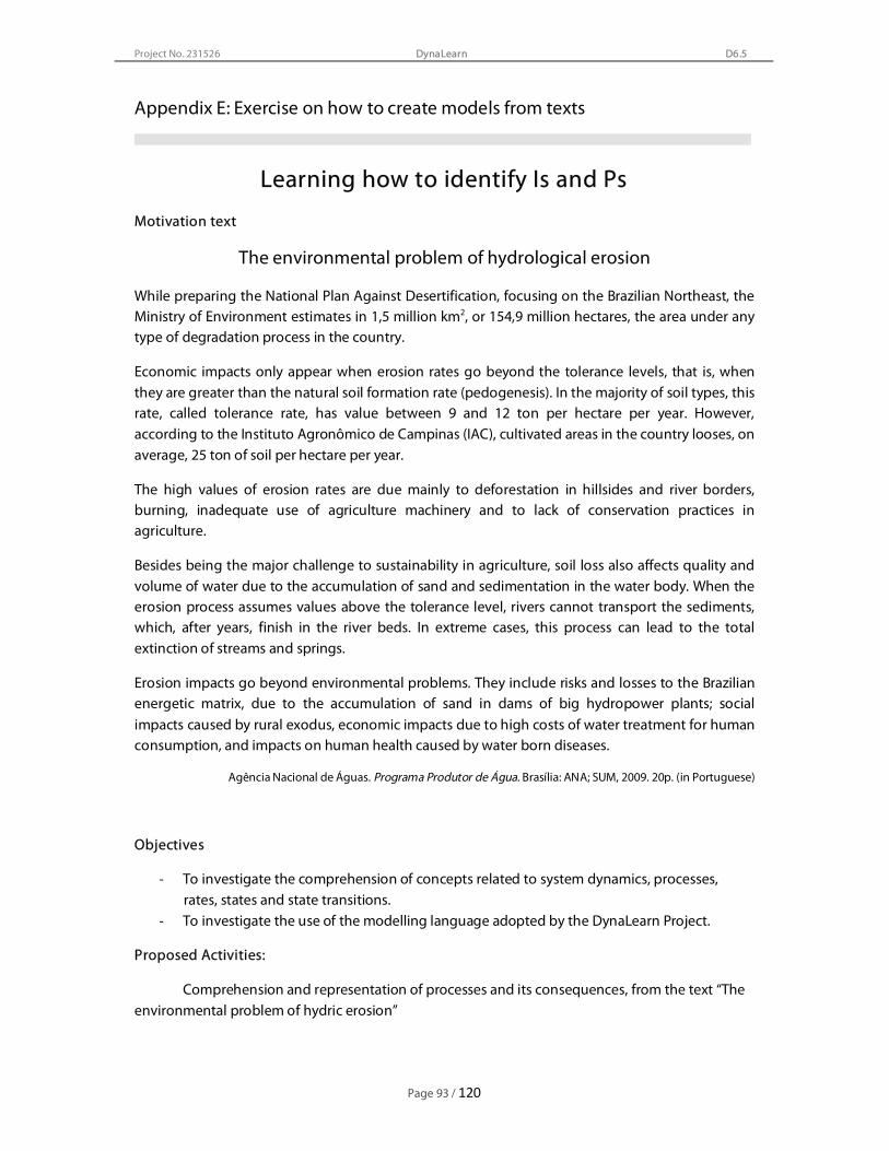
Project No. 231526

/ 120

DynaLearn D6.5

Appendix E: Exercise on how to create models from texts

Learning how to identify Is and Ps

Motivation text

The environmental problem of hydrological erosion

While preparing the National Plan Against Desertification, focusing on the Brazilian Northeast, the Ministry of Environment estimates in 1,5 million km2, or 154,9 million hectares, the area under any type of degradation process in the country.

Economic impacts only appear when erosion rates go beyond the tolerance levels, that is, when they are greater than the natural soil formation rate (pedogenesis). In the majority of soil types, this rate, called tolerance rate, has value between 9 and 12 ton per hectare per year. However, according to the Instituto Agronômico de Campinas (IAC), cultivated areas in the country looses, on average, 25 ton of soil per hectare per year.

The high values of erosion rates are due mainly to deforestation in hillsides and river borders, burning, inadequate use of agriculture machinery and to lack of conservation practices in agriculture.

Besides being the major challenge to sustainability in agriculture, soil loss also affects quality and volume of water due to the accumulation of sand and sedimentation in the water body. When the erosion process assumes values above the tolerance level, rivers cannot transport the sediments, which, after years, finish in the river beds. In extreme cases, this process can lead to the total extinction of streams and springs.

Erosion impacts go beyond environmental problems. They include risks and losses to the Brazilian energetic matrix, due to the accumulation of sand in dams of big hydropower plants; social impacts caused by rural exodus, economic impacts due to high costs of water treatment for human consumption, and impacts on human health caused by water born diseases.

Agência Nacional de Águas. Programa Produtor de Água. Brasília: ANA; SUM, 2009. 20p. (in Portuguese)

Objectives

- To investigate the comprehension of concepts related to system dynamics, processes, rates, states and state transitions.

- To investigate the use of the modelling language adopted by the DynaLearn Project.

Proposed Activities:

Comprehension and representation of processes and its consequences, from the text “The environmental problem of hydric erosion”

Project No. 231526

/ 120

DynaLearn D6.5

Guided study about the text “The environmental problem of hydric erosion”

1. First paragraph

“In the elaboration of the National Plan of Fight against Desertification, which main focus is the Brazilian Northeast, the Environment Ministry estimated in 1,5 millions of km2, or 154,9 million of hectares, the country’s area that present some degradation process.” Objective: Identify Entity, Quantity, and Process. Entity = object that identifies the system of interest [remember that system an unit that consists of objects and relation between them] Quantity = variable property of an object [remember that certain properties are invariable (ex. Name), and others can change according to time (ex. Number of inhabitants)]

Erosão Hid LS4 vs1 increasing vs01.eps Erosão Hid LS4 vs1 decreasing.eps

Process = mechanism capable of causing change in the system, capable of transforming a state of the system in another one [ remember that changes in the system can always be explained by some mechanism, for example, natural area can be degraded]

Exercises:

(a) Indentify the central issues in the text of this paragraph.

Answer: Desertification, environmental degradation in Brazil.

Project No. 231526

/ 120

DynaLearn D6.5

(b) In the hypothesis of building a qualitative model about the subject addressed in the text, identify, among the selected elements of the cited paragraph, what could be considered as Entity or Quantity, using the letters E and Q, respectively. ( ) National Plan ( ) area ( ) Northeast ( ) Environment Ministry ( ) country Answers: E, Q, E, E, E

2. Second paragraph

“Economic impacts only appear when erosion rates go beyond the tolerance levels, that is, when they are greater than the natural soil formation rate (pedogenesis). In the majority of soil types, this rate, called tolerance rate, has value between 9 and 12 ton per hectare per year. However, according to the Instituto Agronômico de Campinas (IAC), cultivated areas in the country looses, on average, 25 ton of soil per hectare per year.”

(a) Defining RATE

- measure of the quantity of variation of a variable, by time unit; the unity that measure the a rate must always have a reference regarding time (ex., space covered per hour, number of children dead per year, soil lost per hectare per year, etc.) [see additional text] A process can present itself in two states: active or inactive. The form of capturing those two situations is to create, respectively, the qualitative values zero and positive (or plus).

(b) Implementing processes

- Processes are represented by the combination of rates with state variables [see additional text]

- The relation between these two quantities is represented by I+ or I- [see additional text]

Project No. 231526

/ 120

DynaLearn D6.5

“EH model vs04 only erosion rate” showing the and the state variable.eps

“EH model vs04 only erosion rate” with a direct influence.eps

(c ) Simulations

Various simulations can be run using this minimal model.

Exploring the initial values:

- Initial values: Amount of soil = <critic,?>; Erosion rate = <zero, ?>, Formation rate = <plus, ?>. - Initial values: Amount of soil = < critic, ?>; Erosion rate = <plus, ?>; Formation rate = <zero, ?> - Initial values: : Amount of soil = < critic, ?>; Erosion rate = <plus, ?>; Formation rate = <plus, ?>

(d) Exploring inequalties

- Initial values: Amount of soil = < critic, ?>; Erosion rate = <plus, ?>; Formation rate = <plus, ?> - Erosion rate > Formation rate - Erosion rate = Formation rate - Erosion rate < Formation rate

3. Third paragraph:

“The high values of erosion rates are due mainly to deforestation in hillsides and river borders, burning, inadequate use of agriculture machinery and to lack of conservation practices in agriculture.”

(a) .Discuss the processes found in this paragraph:

- Is deforestation a process? - Burning? (Combustion?) - Use? Utilization?

(b) Convenience in including all the processes

Project No. 231526

/ 120

DynaLearn D6.5

I+ (deforested area, deforestation rate)

I+ (burned area, combustion rate)

I+ (utilized area, use rate)

[Observe that if the option is of process, we have to introduce one more quantity – the rate – what raises the complexity of the model]

(c) Determine the way of representing the factors cited in the text

Two options: place processes and/or just variables that will be linked by proportionalities (and make the exogenous variable). [However, as we didn’t introduce the proportionalities, let’s select only the deforestation process].

(d) Make the students build a simple model about deforestation:

-demonstrate that the entity Soil would not be appropriate to host deforestation process; suggest the creation of the entity Vegetation and the configuration ‘on’, in order to establish the structural relation between these two entities: ‘Vegetation on Soil’;

- Define Deforestation rate (quantitative space zp) and, as state variable, Deforested area (quantitative space {zero, small, critic, big} = zscb)

[Note that the critic value included in the quantitative space can be productive, in the sense that there is a critical point from which the resilience stops working and so the soil could enter in an irreversible degradation state. Another model could explore this concept…]

[Note, as well, that instead of ‘Deforested area’, the quantity ‘Area covered by vegetation’ could be used, receiving a negative influence (I-) from the rate; a third option could also represent both state variables, with a I+ and a I- to each of them]

(e) Create a link between the two representations (deforestation and erosion/pedogenesis)

- Add the process pedogenesis, or soil formation, mentioned in the 2nd paragraph, in order to get a complete picture of the opposite processes.

- Define what qualitative proportionality is [see additional text]

- Show why in this case it wouldn’t be appropriate use the direct influence (I), but the proportionality (P) to make the link between deforested area and erosion rate.

- Implement the model P+(Erosion rate, Deforested area).

You should obtain the following Figure:

Project No. 231526

/ 120

DynaLearn D6.5

Erosão Híd vs06 deforestation erosion and formation.eps

(f) Simulations with this model:

- Consider the following qualitative values:

Deforestation rate = <plus, ?>; Deforested area = < zero, ?>; Erosion rate = <zero, Formation rate = <plus, ?>; Amount of soil = <critic, ?>

Erosão Híd vs06 desm eros e form vhd 1.eps Erosão Híd vs06 desm eros e form vhd 2.eps

Project No. 231526

/ 120

DynaLearn D6.5

Run other simulations:

- Deforestation rate = <zero, ?>; Deforested area = < zero, ?>; Erosion rate = <zero, ?>; Formation rate = <plus, ?>; Amount of soil = <critic, ?>

- Deforestation rate = <plus, ?>; Deforested area = < zero, ?>; Erosion rate = <zero, ?>; Formation rate = <zero, ?>; Amount of soil = < critic,?>

Outcomes of this model:

Is there any relation (that is, any feedback) between Deforested area and Formation rate? Does it make any ecological sense? How it should be, positive or negative?

Implement the feedback loop(s) and run simulations, exploring the new model.

4. Fifith paragraph:

[Note that will jump the fourth paragraph, as the model would require LS5 or LS6 – see below]

“The impacts of the erosion without control go beyond the environmental area. It includes risks and prejudice to the Brazilian energetic matrix, due to the siltation of the reservoirs of big hydroelectric plants; social impacts due to the rural exodus, economic impacts due to high costs of water treatment for human consumption, and impacts on human health caused by water born diseases.”

(a) Again, discuss the mentioned proceedings: siltation, electric energy production, rural exodus (migration), water treatment, diseases (of hydric) vehiculation.

To simplify the model, let’s consider only one variable capable of representing each of these parts, of the text:

TEXT

MODEL ENTITY QUANTITY

Siltation River Siltated area Rural exodus (migration) Population Migrantes number Water treatment River Water treatment costs Diseases (hydric) vehiculation River Pathological agents

(b) Build a model that completes the previous one, in a way that includes the entities and respective quantities. Also include the question that involves the hydroelectric power plants.

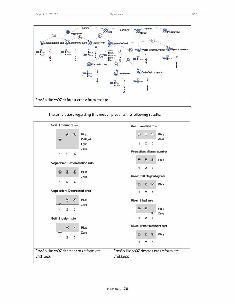
Project No. 231526

/ 120

DynaLearn D6.5

Erosão Híd vs07 deforest eros e form etc.eps

The simulation, regarding this model, presents the following results:

Erosão Híd vs07 desmat eros e form etc vhd1.eps

Erosão Híd vs07 desmat eros e form etc vhd2.eps

Project No. 231526

/ 120

DynaLearn D6.5

5. Fourth paragraph: “Beyond being the greatest challenge regarding agriculture sustainability, the loss of soil also affects considerably the water quality and volume, due to the sedimentation and siltation processes. When the erosive process assumes values above the tolerance rate, the water courses can no longer carry those sediments that, as years go by, end up being deposited in its beds. In extreme cases, these process can culminate in the total extinction of small water streams and springs.”

This text contains a part that shows a conditional knowledge, a phenomenon that depends of certain conditions to happen. “When the erosive process assumes values above the tolerance rate, the water courses can no longer carry those sediments that, as years go by, end up being deposited in its beds.”

To model this phenomenon (“can no longer carry those sediments that, as years go by, end up being deposited in its beds”), its necessary that two alternate situation are represented:

IF Erosion rate < or = the Formation rate (or tolerance), THEN Transport rate > Sedimentation rate (making the sediments be carried);

IF Erosion rate > or = the Formation rate (or tolerance), THEN Transport rate < Sedimentation rate (making the sediments be carried).

To implement this idea, its necessary to use LS5 or LS6. This is subject for another exercise.

ooooooooooooooooooooooooooooooooooooooooooooooooooooooooooooooo

OPTIONAL ACTIVITES EXPLORING THE TEXT

(A) give examples of how the degradation process works, cited in the first paragraph:

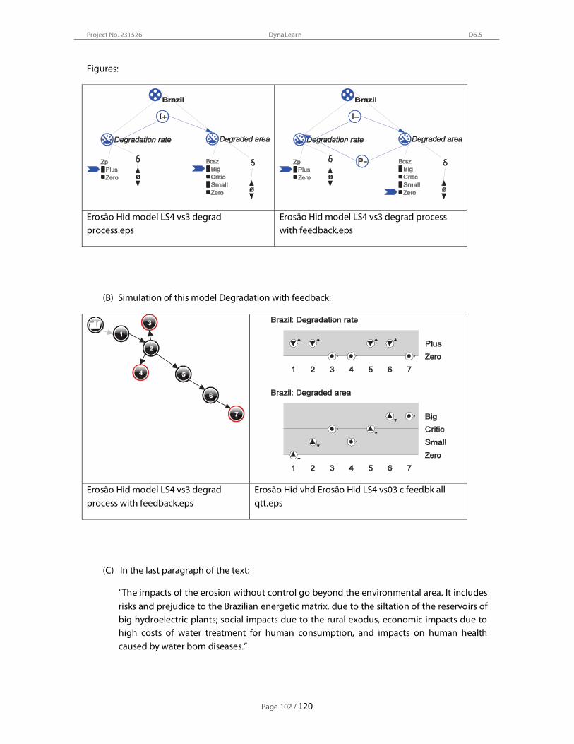
Project No. 231526

/ 120

DynaLearn D6.5

Figures:

Erosão Hid model LS4 vs3 degrad process.eps

Erosão Hid model LS4 vs3 degrad process with feedback.eps

(B) Simulation of this model Degradation with feedback:

Erosão Hid model LS4 vs3 degrad process with feedback.eps

Erosão Hid vhd Erosão Hid LS4 vs03 c feedbk all qtt.eps

(C) In the last paragraph of the text:

“The impacts of the erosion without control go beyond the environmental area. It includes risks and prejudice to the Brazilian energetic matrix, due to the siltation of the reservoirs of big hydroelectric plants; social impacts due to the rural exodus, economic impacts due to high costs of water treatment for human consumption, and impacts on human health caused by water born diseases.”

Project No. 231526

/ 120

DynaLearn D6.5

In the hypothesis of building a qualitative model about the issue presented in that text, identify, among the elements selected in the cited paragraph, what could be treated as Entity or Process, using, respectively, the letters E and P:

( ) Energetic matrix ( ) Treatment (water)

( ) Reservoirs ( ) Vehiculation (water)

( ) Erosion ( ) Hydroeletric power plants

( ) Water ( ) Distrubution (water)

( ) Siltation ( ) Population

Answer: first column: E, E, P, E, P; second column: P, P, P, E, P, E

(D ) OPTIONAL.

The quantity rate can also have quantitative space {minus, zero, plus}, to represent the combination of two rates, one with positive influence and other with negative [see below].

(E) OPTIONAL.

After reading the text and identifying the causality relations, write, in the appropriate column in the box below, causes and its immediate effects, following the given examples.

# CAUSES EFFECTS

1 Hills deforestation High erosion rates

2 Riverbanks deforestation High erosion rates

(...)

(etc.) (etc.)

Project No. 231526

/ 120

DynaLearn D6.5

GOING FROM LS4 TO LS6

Objective:

Demonstrate how to represent in LS6, models developed in LS4

Materials:

Water Erosion LS4.hgp

Procedure:

1. To study the LS4 model;

2. Search for model patterns in the LS4 model;

3. To build LS6 model:

a. Put model patterns found in LS4 model in different model fragments, you can start with processes;

b. Create static model fragments to link the different patterns;

c. Create scenarios, you can start with simple scenarios and go to scenarios more complex with more variables.

Implementation of water erosion LS4 model in LS6

Following the proposal commented above, the objective is to split the model presented in LS4 and build a library of model fragments, where each fragment contains a part of the knowledge about Water Erosion. Different scenarios can be elaborated from what it is possible to run simulations exploring different combinations of the parts or the totality of model fragments present in the library.

Planning the LS6 model

STEP 1: To move a model from LS4 to LS6 is to identify all the basic model patterns in the LS4 model

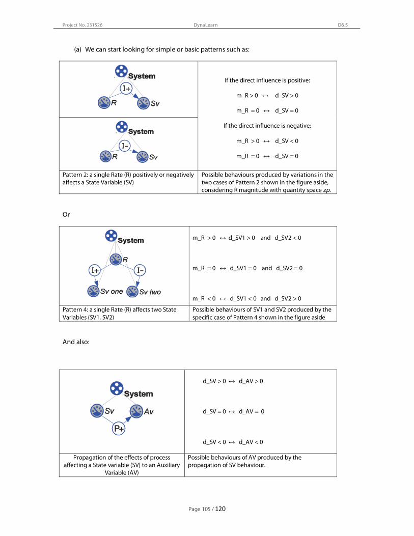
Project No. 231526

/ 120

DynaLearn D6.5

(a) We can start looking for simple or basic patterns such as:

If the direct influence is positive:

m_R > 0 ļ d_SV > 0

m_R = 0 ļ d_SV = 0

If the direct influence is negative:

m_R > 0 ļ d_SV < 0

m_R = 0 ļ d_SV = 0

Pattern 2: a single Rate (R) positively or negatively affects a State Variable (SV)

Possible behaviours produced by variations in the two cases of Pattern 2 shown in the figure aside, considering R magnitude with quantity space zp.

Or

m_R > 0 ļ d_SV1 > 0 and d_SV2 < 0

m_R = 0 ļ d_SV1 = 0 and d_SV2 = 0

m_R < 0 ļ d_SV1 < 0 and d_SV2 > 0

Pattern 4: a single Rate (R) affects two State Variables (SV1, SV2)

Possible behaviours of SV1 and SV2 produced by the specific case of Pattern 4 shown in the figure aside

And also:

d_SV > 0 ļ d_AV > 0

d_SV = 0 ļ d_AV = 0

d_SV < 0 ļ d_AV < 0

Propagation of the effects of process affecting a State variable (SV) to an Auxiliary

Variable (AV)

Possible behaviours of AV produced by the propagation of SV behaviour.

Project No. 231526

/ 120

DynaLearn D6.5

Figure Water Erosion LS4

Here it is important to notice that sometimes the considerations of which pattern is represented deponds on the definitions and the modelling choices made by the modeller

STEP 2: create the entity tree with the objects of the system to be modelled:

Entity tree

1 – It is possible to represent each process in separate model fragments

2 – It is possible to

represent the effects of processes in other model fragments

3 – It is possible to represent other effects and their propagations in separate model fragments

Project No. 231526

/ 120

DynaLearn D6.5

STEP 3: create a static model fragment “Fm01 vegetation contains deforested area”

Fm01 vegetation contains deforested area

Step 4: create the Process model fragment “Fm02 vegetation has deforestation rate

Fm02 vegetation has deforestation rate

Step 5: create a scenario “Scen01 deforestation”

Scen01 deforestation

Step 6: simulate the scenario and answer the following questions:

a) How much initial states? ___________

b) How much final states? ________________

c) What is the total amount of states? _____________

d) Choose one path to describe the behaviour of the variable “ Deforested area”

Project No. 231526

/ 120

DynaLearn D6.5

Step 7: create the static model fragment “Fm03 deforested area affect erosion rate”

Fm03 deforested area affect erosion rate

Step 8: create a scenario “Scen02 deforestation affects erosion”

Scen02 deforestation affects erosion


a) How much initial states? ___________

b) How much final states? ________________


d) Choose one path to describe the behaviour of the variable “Erosion rate”

Project No. 231526

/ 120

DynaLearn D6.5

Step 10: create the static model fragment “Fm04 deforestation affects soil formation”

Fm04 deforestation affects soil formation

Step 11: create the process model fragment “Fm05 erosion rate affects amount of soil”

Fm05 erosion rate affects amount of soil

Step 12: create the model fragment “Fm06 soil formation affects amount of soil”

Fm06 soil formation affects amount of soil

Step 13: create the scenario “Scen03 amount of soil”

Project No. 231526

/ 120

DynaLearn D6.5

Scen03 amount of soil


a) How many initial states? ___________

b) How many final states? ________________



Step 15: various simulations can be run using this minimal Scenario and it is possible to create similar scenarios just changing the initial values

Exploring the initial values: - Initial values: Amount of soil = <critic,?>; Erosion rate = <zero, ?>, Formation rate = <plus, ?>. - Initial values: Amount of soil = < critic, ?>; Erosion rate = <plus, ?>; Formation rate = <zero, ?> - Initial values: Amount of soil = < critic, ?>; Erosion rate = <plus, ?>; Formation rate = <plus, ?>

Exploring inequalties

- Initial values: Amount of soil = < critic, ?>; Erosion rate = <plus, ?>; Formation rate = <plus, ?> - Erosion rate > Formation rate - Erosion rate = Formation rate - Erosion rate < Formation rate

Step 16: now it is up to you to create a scenario using all variables created until now, name it as “Scen04 deforestation affects soil”

Scen04 deforestation affects soil

Project No. 231526

/ 120

DynaLearn D6.5


a) How many initial states? ___________

b) How many final states? ________________



Step 18: create new model fragments and create a scenario using all variables created until now, name it as “Scen05 soil affects river and population”

Scen05 soil affects population and river

Didactic material prepared by Paulo Salles and FUB’s team for DynaLearn WP6 and WP7 May, 2010

Project No. 231526

/ 120

DynaLearn D6.5

Project No. 231526

/ 120

DynaLearn D6.5

Appendix F: A qualitative model of the logistic curve

A qualitative model of the logistic curve

Objectives

• To present a qualitative model of the logistic curve; • To illustrate how to explore correspondences and conditional knowledge in order

to implement a complex model.

AN IMPORTANT PATTERN FOR ECOLOGY: THE LOGISTICS

The system behaviour captured by the logistic curve is shown in the following figure:

The logistic curve (from Wikipedia: http://en.wikipedia.org/wiki/File:Logistic-curve.svg)

The behaviour can be divided in three main sections: initially the variable grows exponentially (from -6 to zero); in zero, where the variable reaches a value that is half of the stabilization value, there is a inflection point, and from thereon, the variable keeps increasing, but a slower rate (from zero to 6); the third section

Project No. 231526

/ 120

DynaLearn D6.5

corresponds to stabilization. In fact, a fourth section can be considered, when the variable is above the stabilization point, when the variable tends to return to the stabilization value.

In ecology, the logistic curve has a great importance, both from the historical point of view, and for theoretical basis for population dynamics, expressing particularly density-dependent populations (cf. Gotelli, 1995, among others). In this context, the variable representing population size has two limit points, where the system behaviour change: K, the carrying capacity, in which the state variable stabilizes, and K/2, the inflection point.

A simple logistic function is described by the equation

N(t) = 1/ 1 + ert

where r is the intrinsic growth rate or the per capita growth rate.

The usual formulae including density dependence was introduced in ecology by Verhulst in 1838 to describe population growth in a resource-limited environment:

dN/dt = rN( 1- N/K)

where K is the carrying capacity, representing the maximum population size that can be supported with the resources available (Gotelli, 1995).

The Model

The model follows the basic system pattern, with an aggregate rate (Net rate) affecting a state variable (Number_of) and an unbalanced situation involving two Auxiliary Variables (Born and Dead). Critical for knowledge representation in the model are the use of correspondences between specific values, and the use of conditional knowledge.

The model consists of one entity, representing a density-dependent population (‘DD Population’), four quantities and eight model fragments:

Logistic Model, all the model fragments

Project No. 231526

/ 120

DynaLearn D6.5

The most relevant model fragments are shown below.

MF01 Population configuration MF02 Population growth process

Correspondences in ‘MF02 Population growth process’ establish the co-occurrence of the values [Number_of = zero; Net rate = zero]; [Number_of = K; Net rate = zero]; [Number_of = above K; Net rate = minus] and all the possible values of Number_of with Net rate = plus.

The use of conditional knowledge is important to set the behaviour of Number of, in each of the stages of the logistic curve , as shown in the model fragments below.

MF02b Number of individuals smaller than the inflection point

MF02c Number of individuals equal to the inflection point

Project No. 231526

/ 120

DynaLearn D6.5

During the first phase, Number_of must be smaller than the value K, and Net rate, <positive, increasing>. For that, Born > Dead is obtained if the former is influenced by a positive proportionality and the latter by a negative one (MF 02b, above). When Number_of equals K, both the Rate is steady and the State variable is increasing (MF 02c, above).

After the inflection point, the proportionalities imposed by Number_of on Born and Dead individuals shall create the conditions for the Net rate to decrease (MF02d, below), and stabilize when the carrying capacity is reached. The last model fragment (MF02f, below) shows that when the state variable is above carrying capacity, the Net rate descreases and stabilizes at K.

MF02d Number of individuals greater than the inflection point

MF02f Number of individuals greater than the carrying capacity

The model fragment MF02a that shows the situation in which Number_of = zero is condition for Born individuals, Dead individuals and Net rate assume the values < zero, zero >. The final equilibrium, when Number_of = K is condition for Net rate assume the values < zero, zero >, is shown in ‘MF02e Number_of equals K’.

Project No. 231526

/ 120

DynaLearn D6.5

A simulation with this model shows the typical logistic behaviour described in the set of model fragments.

Scenario 03 starts the simulation with Number_of below the inflection point

State graph obtained in a simulation starting with Scenario 03, showing one initial state (1) e one end state (6)

Causal model in State 1, in a simulation starting with Scenario 03.

Causal model in state 3, same simulation. .

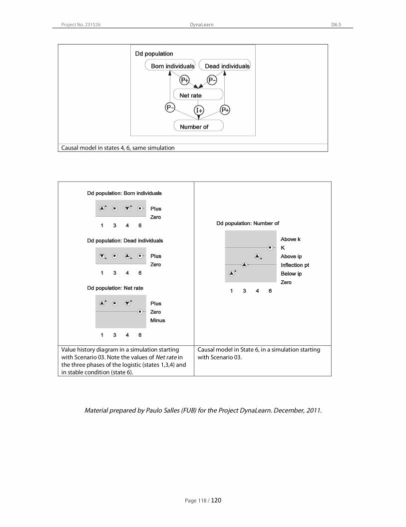
Project No. 231526

/ 120

DynaLearn D6.5

Causal model in states 4, 6, same simulation

Value history diagram in a simulation starting with Scenario 03. Note the values of Net rate in the three phases of the logistic (states 1,3,4) and in stable condition (state 6).

Causal model in State 6, in a simulation starting with Scenario 03.

Material prepared by Paulo Salles (FUB) for the Project DynaLearn. December, 2011.

Project No. 231526

/ 120

DynaLearn D6.5

Appendix G: Glossary of System Dynamics Terminology

systems thinking: Thought process that involves 1) seeing interrelationships (feedback loops) instead of linear cause-effect chains, and 2)seeking processes of change over time rather than snapshots. Systems thinking involves understanding many concepts of system dynamics, most notably, feedback. It helps thinkers see things on three levels: events, patterns of behaviour, and system structure. systems archetypes: A system dynamics structure that is common to many systems. See also generic structures. generic structure: A structure that can be applied across different settings due to fundamentally same underlying structures and relationships. mental model: A model representing the relationships and assumptions about a system held in a person’s mind. Mental models are often correct in system structure, but frequently draw wrong conclusions about system behaviour. exponential growth/decay: Behaviour that occurs when the rate of growth depends on the size of the stock at that point in time. As the stock gets larger, its growth gets progressively faster. Or, for decay, as the stock gets smaller, the decay gets progressively slower. Exponential growth/decay has a doubling time. Associated with positive feedback, or a half-life associated with decay. asymptotic growth/decay: Goal-seeking behaviour produced by negative feedback. The stock of the system moves towards the goal, slowing down as it approaches the goal. delay: A phenomenon where the effect of one variable on another does not occur immediately. Delays result from decisions often require a long period of time to be effective. Delays can result in overshoot or oscillation. cyclical behaviour: See oscillation, overshoot and collapse oscillation: Behaviour exhibited by a second-order or higher-order system in which the stock value moves sinusoidally over time. Three types of oscillation include sustained, where the amplitude is always constant; expanding, where the amplitude increases over time; and dampened, where the amplitude decreases over time. overshoot and collapse: A system that grows beyond a sustainable condition (overshoot), reduces the basis for sustained existence, then collapses below the level that might have been sustained. Example: fishing rates that exceed the replenishment rate resulting in a collapse of the fishing population. S-shaped growth: Growth that exhibits behaviour in the shape of the letter “S.” It expands rapidly at first, then slows down as stock approaches its maximum value. S-shaped growth is caused by a shift in loop dominance from positive to negative feedback. stability: Behaviour exhibited by a system that returns to its initial condition after being disturbed. In an unstable system, a disturbance is amplified, leading increased growth or oscillation. A stable oscillation is one at a constant amplitude, as in a clock pendulum. steady-state: A behaviour pattern that is repetitive with time and in which the behaviour in one time period is of the same nature as any other period.

dynalearn curriculum for environmental science - uva · among a number of definitions of...

Documents