dynamic analysis and design of mooring linesdynamic analysis and design of mooring lines michael...

Dynamic Analysis and Design of Mooring Lines

Michael Olivier Chrolenko

Marine Technology

Supervisor: Carl Martin Larsen, IMT

Department of Marine Technology

Submission date: June 2013

Norwegian University of Science and Technology

Dynamic Analysis and Design of Mooring Lines

Master Thesis

Michael Chrolenko

Marine Structures and Hydrodynamics

Spring 2013


Department of Marine Technology

Supervisor MTS: Professor Carl M. LarsenSupervisor DNV: Erling Lone

Preface

This master thesis concludes the Master Degree program of Marin Technology at the NorwegianUniversity of Science and Technology (NTNU). This thesis has been carried out from Januaryto June 2013 in cooperation with DNV.

First of all I would like to thank DNV, and especially my supervisor Erling Lone for guiding methrough this semester. He has given me continues help, and pointed me in the right directionwhen getting of track. The help, time spent, and the lectures given are most appreciated. Thee�ort and patience towards me has been outstanding, especially when repeating problems whichwere not fully understood.

Would also like to thank my supervisor here on MTS, Carl Marin Larsen. Apart from thescheduled appointments, his door has always been open for consultation on my master thesis.He has also taken initiative and signed me up for di�erent program courses given by MARINTEK,as well as providing me with relevant articles. His help regarding RIFLEX problems are greatlyappreciated.

A warm thank is also given to MARINTEK, especially Karl Erik Kaasen. He has been most help-ful in discussing di�erent topics related to MIMOSA by email and scheduled meetings throughoutthis semester. Elizabeth Passano and Knut Mo at MARINTEK are acknowledged for includingme in the SIMA course, and for meeting me in person when help was needed. Would also liketo thank MARINTEK for providing me with the programs and licenses used for this masterthesis.

This master thesis has been quite interesting and very educational. Leaning about all the dif-ferent computation programs has been challenging, but very useful in preparing me for real lifework. Overall I'm quite satis�ed and pleased for choosing this task given by DNV.

MTS, Trondheim, 3rd June 2013

i

NTNU Trondheim


Faculty of Engineering Science and Technology

Department of MarineTechnology

M.Sc. thesis 2013

for

Stud.tech. Michael Chrolenko

DYNAMIC ANALYSIS AND DESIGN OF MOORING LINES

Mooring line response may be calculated in frequency domain (FD) or in time domain (TD),

and the choice of method is normally a compromise between accuracy and computational

effort. FD methods are faster than the use of TD simulations, and in many cases provide

satisfactory results. Due to the non-linear and dynamic behaviour of mooring lines, TD

simulations provide the most accurate results, but are considerably more time-consuming and

introduce statistical uncertainty to the calculations due to the stochastic nature of the response.

For fatigue calculations, a large number of sea states must be considered, and FD is therefore

the preferred choice given that the response properties are satisfactory modelled.

At shallow water depths (≤ 100 m), catenary moorings without buoyancy elements or clump

weights are considered to have a quasi-static behaviour. This implies that the tension may be

calculated from a static representation of the mooring line, and calculation methods as e.g.

MIMOSA QS (FD) or SIMO (TD) are expected to yield satisfactory results. Whereas this is

often the case for the windward lines (i.e. pointing towards the incoming waves), the response

properties of the leeward lines (i.e. pointing away from the incoming waves) of turret moored

FPSOs are different and not necessarily well captured by a quasi-static model.

In most cases, the windward lines are the critical lines with respect to extreme response for

moored structures, due to both a high mean tension and a large dynamic contribution. For

estimation of fatigue damage, on the other hand, only the dynamic contributions are

considered. For turret moored structures the largest dynamic response is often seen in the

leeward lines, and this effect increases with the longitudinal distance from COG to the turret.

Thus, a study addressing the goodness for such units of the frequency domain methods (both

QS and FEM) compared to fully dynamic time domain analyses would be of high value to the

industry.

The main scope of the thesis will be to perform a comparison of results for mooring line

analyses in frequency domain (FD) and time domain (TD), for a turret moored FPSO with

catenary moorings at 100m water depth. The following software (all developed by

MARINTEK) and analysis methods should be compared:

MIMOSA QS method - Frequency domain, quasi-static

MIMOSA FEM method - Frequency domain, dynamic (linearized)

SIMO Time domain, quasi-static

RIFLEX /3/ Time domain, dynamic and fully non-linear

SIMA Program to take care of communication between programs

The main concern of the comparison will be to investigate differences in response calculations

for leeward lines, for the purpose of estimating fatigue damage in a given short-term sea state.

NTNU Faculty of Marine Technology

Norwegian University of Science and Technology Department of Marine Structures

The work may show to be more extensive than anticipated. Some topics may therefore be left

out after discussion with the supervisor without any negative influence on the grading.

The candidate should in her/his report give a personal contribution to the solution of the

problem formulated in this text. All assumptions and conclusions must be supported by

mathematical models and/or references to physical effects in a logical manner.

The candidate should apply all available sources to find relevant literature and information on

the actual problem.

The report should be well organised and give a clear presentation of the work and all

conclusions. It is important that the text is well written and that tables and figures are used to

support the verbal presentation. The report should be complete, but still as short as possible.

The final report must contain this text, an acknowledgement, summary, main body,

conclusions and suggestions for further work, symbol list, references and appendices. All

figures, tables and equations must be identified by numbers. References should be given by

author name and year in the text, and presented alphabetically by name in the reference list.

The report must be submitted in two copies unless otherwise has been agreed with the

supervisor.

The supervisor may require that the candidate should give a written plan that describes the

progress of the work after having received this text. The plan may contain a table of content

for the report and also assumed use of computer resources.

From the report it should be possible to identify the work carried out by the candidate and

what has been found in the available literature. It is important to give references to the

original source for theories and experimental results.

The report must be signed by the candidate, include this text, appear as a paperback, and - if

needed - have a separate enclosure (binder, DVD/ CD) with additional material.

The work will be carried out in cooperation with Det Norske Veritas, Trondheim

Contact person at DNV is Erling Neerland Lone

Supervisor at NTNU is Professor Carl M. Larsen

Carl M. Larsen

Submitted: January 2013

Deadline: 10 June 2013

Abstract

This master thesis presents a comparison study, where the main focus has been to assess ifsimpli�ed methods can be used for analysing mooring lines for a turret moored FPSO in shallowwaters. The MIMOSA program applies frequency domain (FD) methods, which is categorizedas a simpli�ed method but with short computation time. Fully non-linear time domain (TD)analysis in RIFLEX, which is a time consuming process, accounts for all non-linear e�ects, andwas assumed throughout this master thesis to yield the best results. It was also necessary toperform mooring line analysis in SIMO to be able to isolate di�erent e�ects between the threecomputation programs. The results were then used to explain the di�erences between the �niteelement method in MIMOSA (MIM-FEM) and RIFLEX (RIF-FEM). The main focus throughoutthis master thesis has been on the leeward line because this line will experience large dynamics,and it will also be the critical line for fatigue damage. The windward line has mainly been usedto compare with the leeward line. For fatigue damage the most important parameters are thestandard deviation (STD) of low- and wave-frequency tension (LF and WF).

When performing a comparison study it is important to assure that the model in MIMOSA,SIMO, and RIFLEX are equivalent. This means that line characteristics, restoring force char-acteristics, environmental forces, motions, equilibrium positions, and pretensions are the samefor all programs. In MIMOSA and SIMO all the 12 mooring lines were modelled, while only thewindward and leeward lines were modelled in RIFLEX. Because RIFLEX needs to get prescribedmotions from SIMO, most of the comparisons in verifying the model were made based on resultsfrom MIMOSA and SIMO.

Comparing the mean equilibrium position between MIMOSA and SIMO exceeded the acceptablerange of 5% di�erence in the model veri�cation process. This di�erence arises because theiteration process in SIMO did not �nd the exact equilibrium position. This resulted in a residualtension force. By performing simple hand calculations, this di�erence equaled the di�erence inmean equilibrium position between MIMOSA and SIMO and was therefore acceptable. In theend one could conclude that all the models were equivalent, and could thus be used for furtheranalysis.

The programming part for this master thesis was quite time consuming. For every program(MIM,SIM,RIF) a batch script was made, which then was combined together with one main batchscript. The various analyses could then be carried out from this main batch �le automatically,and Matlab was then used to post process the results.

The results showed that a quasi-static representation is acceptable when calculating the STD ofLF tension. The di�erence between MIM-FEM and RIF-FEM for STD of LF tension was 0,13%for the leeward line, and -3,58% for the windward line, meaning that MIM-FEM slightly underpredicts the STD of LF tension for the windward line.

vii

For the turret moored FPSO analysed in this master thesis, a quasi-static representation of themooring lines is not recommended for the leeward and windward line because the STD of WFtension will be too conservative. The di�erence between the simpli�ed FEM in MIMOSA andthe fully non-linear TD analysis in RIFLEX was -22,48% for the leeward line, and -16,66% forthe windward line. The di�erence here is mainly caused by the linearisation methods used inMIMOSA to account for geometrical sti�ness and dynamic e�ects (drag and inertia forces actingon the mooring line). Using the simpli�ed FEM in MIMOSA one will under predict the STDof WF tension for the windward and leeward line, and therefore under predict the results in theestimation of fatigue life in the mooring lines.

viii

Sammendrag

Denne master oppgaven presenterer en sammenlignings studie, hvor hoved fokuset er å esti-mere om forenklede metoder kan brukes til fortøynings analyse av turret forankret FPSO pågrunt vann. MIMOSA programmet bruker frekvensplan (FD) metoder, som er kategorisert forå være forenklede metoder som bruker kort beregningstid. Full ikke-lineær tidsplan (TD) analy-se i RIFLEX er tidkrevende fordi RIFLEX betrakter alle ikke-lineære e�ekter. Gjennom dennemaster oppgaven så antas det at RIFLEX gir de beste resultatene. Det var også nødvendig ågjennomføre fortøynings analysen i SIMO for å kunne skille mellom ulike e�ekter for disse trenevnte programmene. Resultatene fra SIMO analysen ble brukt til å forklare forskjeller mellomelement metoden i MIMOSA (MIM-FEM) og element metoden i RIFLEX (RIF-FEM). Hoved-fokuset gjennom denne master oppgaven har vært å se på le-linen fordi denne fortøyningslinenvil oppleve stor dynamikk samt også være den kritiske linen for utmattingsskade. Lo-linen harhovedsakelig blitt brukt til sammenligninger med le-linen. De viktigste parameterne når man serpå utmattingsskade er standard avvik (STD) for lav- og bølgefrekvent strekk (LF og WF).

Når en sammenlignings studie skal utføres er det viktig å forsikre seg om at alle modellene i de treprogrammene; MIMOSA, SIMO og RIFLEX er ekvivalente. Dette innebærer at line karakteris-tikk, fjæringskraft karakteristikk, miljø krefter, bevegelser, likevekts posisjoner, og forspenningerer like for alle programmene. I MIMOSA og SIMO så er alle de 12 fortøyningslinene modellert,mens i RIFLEX er kun lo- og le-linen modellert. Fordi RIFLEX for bevegelsen sin fra SIMO såvil mye av sammenligningen i veri�serings prosessen være basert på resultatene fra MIMOSA ogSIMO.

Når likevekts posisjonen mellom MIMOSA og SIMO ble sammenlignet i veri�serings prosessen såovergikk denne sammenligningen den akseptable grensen, hvor akseptabel grense er på mindre en5% forskjell. Forskjellen oppstår fordi SIMO ikke klarte å �nne den eksakte likevekts posisjonen.Dette resulterte i en restkraft. Ved å utføre en enkel håndberegning ble det vist at denne restkraftforskjellen er lik forskjellen i likevekts posisjonen mellom MIMOSA og SIMO. Konklusjonen iveri�serings prosessen ble at alle modellene er ekvivalente og kan brukes videre i prosjektet.

Programmerings delen i denne master oppgaven var meget tidkrevende. For hvert program (MIM,SIM, RIF) ble det laget et batch-skript, som videre ble koblet sammen med et hoved batch-skript. De forskjellige analysene kunne nå bli kjørt fra dette hoved skriptet automatisk. Når alleanalysene er ferdige ble Matlab brukt for prosessering av resultatene.

Resultatene viste at en kvasi-statisk representasjon er akseptabel for beregningen av STD avLF strekk. Forskjellen mellom MIM-FEM og RIF-FEM for STD av LF strekk var på 0,13% forlo-linen, og -3,58% for le-linen. Dette betyr at MIM-FEM så vidt under estimerer STD av LFstrekk for le-linen.

I denne master oppgaven ble en turret forankret FPSO analysert, og en kvasi-statisk representa-sjon av fortøyningslinene er ikke anbefalt. Dette er fordi en slik representasjon av lo- og le-linen vilgi for konservative resultater. Forskjellen mellom den forenklede element metoden i MIMOSA ogfull ikke-lineær TD analyse i RIFLEX var på -22,48% for lo-linen, og -16,66% for le-linen. Hovedforskjellen kommer av lineariserings prosessen som foregår i MIMOSA som skal betrakte geome-trisk stivhet og dynamiske e�ekter (drag og masse krefter som virker på fortøyningslinen). Vedå bruke den forenklede element metoden i MIMOSA vil man under estimere STD av WF strekkfor lo- og le-linen, som igjen vil under estimere utmattings levetiden til fortøyningslinene.

ix

Contents

Preface . . . . . . . . . . . . . . . . . . . . . . . . . . . . . . . . . . . . . . . . . . . . i

Abstract . . . . . . . . . . . . . . . . . . . . . . . . . . . . . . . . . . . . . . . . . . . . vii

Sammendrag . . . . . . . . . . . . . . . . . . . . . . . . . . . . . . . . . . . . . . . . . ix

Nomenclature . . . . . . . . . . . . . . . . . . . . . . . . . . . . . . . . . . . . . . . . . xvii

1 Introduction 1

1.1 Background for master thesis . . . . . . . . . . . . . . . . . . . . . . . . . . . . . 2

2 Mooring System - General Theory 3

2.1 Mooring/Anchor Lines . . . . . . . . . . . . . . . . . . . . . . . . . . . . . . . . . 3

2.1.1 Drag Forces and Damping . . . . . . . . . . . . . . . . . . . . . . . . . . . 5

2.1.2 Sti�ness . . . . . . . . . . . . . . . . . . . . . . . . . . . . . . . . . . . . . 6

2.2 Separate and Coupled Analysis . . . . . . . . . . . . . . . . . . . . . . . . . . . . 7

2.3 Fatigue Damage . . . . . . . . . . . . . . . . . . . . . . . . . . . . . . . . . . . . . 8

3 Modelling Procedure 12

3.1 Model Implementation . . . . . . . . . . . . . . . . . . . . . . . . . . . . . . . . . 12

3.2 Case Parameter Study . . . . . . . . . . . . . . . . . . . . . . . . . . . . . . . . . 14

3.3 Model Veri�cation . . . . . . . . . . . . . . . . . . . . . . . . . . . . . . . . . . . 15

3.3.1 Mean Environmental Forces . . . . . . . . . . . . . . . . . . . . . . . . . . 16

3.3.2 Anchor Coordinates and Pretension . . . . . . . . . . . . . . . . . . . . . 17

3.3.3 "Mean" Position (equilibrium) . . . . . . . . . . . . . . . . . . . . . . . . 18

3.3.4 "Mean" tension . . . . . . . . . . . . . . . . . . . . . . . . . . . . . . . . . 19

3.3.5 Line Characteristics . . . . . . . . . . . . . . . . . . . . . . . . . . . . . . 19

3.3.6 Restoring Force Characteristics . . . . . . . . . . . . . . . . . . . . . . . . 20

3.3.7 Conclusion - Model veri�cation . . . . . . . . . . . . . . . . . . . . . . . . 21

4 Program Structure 23

4.1 MIMOSA, SIMO, RIFLEX (MSR) Script - Main batch script . . . . . . . . . . . 23

4.2 MIMOSA . . . . . . . . . . . . . . . . . . . . . . . . . . . . . . . . . . . . . . . . 24

4.3 SIMO . . . . . . . . . . . . . . . . . . . . . . . . . . . . . . . . . . . . . . . . . . 25

4.4 RIFLEX . . . . . . . . . . . . . . . . . . . . . . . . . . . . . . . . . . . . . . . . . 27

4.5 Post Processing - Matlab . . . . . . . . . . . . . . . . . . . . . . . . . . . . . . . . 28

5 Program Theory 29

5.1 MIMOSA . . . . . . . . . . . . . . . . . . . . . . . . . . . . . . . . . . . . . . . . 30

5.1.1 LF tension - Only Quasi-Statically . . . . . . . . . . . . . . . . . . . . . . 30

5.1.2 WF tension - General . . . . . . . . . . . . . . . . . . . . . . . . . . . . . 31

xi

5.1.3 WF tension - QS . . . . . . . . . . . . . . . . . . . . . . . . . . . . . . . . 325.1.4 WF tension - FEM . . . . . . . . . . . . . . . . . . . . . . . . . . . . . . . 325.1.5 Non-linear WF tension - FEM . . . . . . . . . . . . . . . . . . . . . . . . . 33

5.2 SIMO . . . . . . . . . . . . . . . . . . . . . . . . . . . . . . . . . . . . . . . . . . 345.2.1 Mooring line tension . . . . . . . . . . . . . . . . . . . . . . . . . . . . . . 34

5.3 RIFLEX . . . . . . . . . . . . . . . . . . . . . . . . . . . . . . . . . . . . . . . . . 345.3.1 Fully non-linear analysis . . . . . . . . . . . . . . . . . . . . . . . . . . . . 355.3.2 Linearised FEM analysis . . . . . . . . . . . . . . . . . . . . . . . . . . . . 35

5.4 Summary of program theory . . . . . . . . . . . . . . . . . . . . . . . . . . . . . . 36

6 Case Study 376.1 System Description . . . . . . . . . . . . . . . . . . . . . . . . . . . . . . . . . . . 376.2 Environmental Condition . . . . . . . . . . . . . . . . . . . . . . . . . . . . . . . 396.3 Calculation Methods . . . . . . . . . . . . . . . . . . . . . . . . . . . . . . . . . . 39

6.3.1 General . . . . . . . . . . . . . . . . . . . . . . . . . . . . . . . . . . . . . 396.3.2 Time Domain . . . . . . . . . . . . . . . . . . . . . . . . . . . . . . . . . . 40

6.4 Filter Design . . . . . . . . . . . . . . . . . . . . . . . . . . . . . . . . . . . . . . 406.5 Fatigue Analysis . . . . . . . . . . . . . . . . . . . . . . . . . . . . . . . . . . . . 44

7 Results and Discussions 467.1 Results . . . . . . . . . . . . . . . . . . . . . . . . . . . . . . . . . . . . . . . . . . 467.2 Windward vs. Leeward line . . . . . . . . . . . . . . . . . . . . . . . . . . . . . . 497.3 Comparison di�erences between methods: STD of WF tension . . . . . . . . . . . 51

7.3.1 Importance of updated line characteristics . . . . . . . . . . . . . . . . . . 517.3.2 Importance of dynamic e�ects . . . . . . . . . . . . . . . . . . . . . . . . . 527.3.3 STD of WF tension: MIM-QS vs MIM-FEM . . . . . . . . . . . . . . . . 537.3.4 STD of WF tension: MIM-FEM vs RIF-FEM . . . . . . . . . . . . . . . . 54

8 Conclusion 558.1 Conclusion from discussions and results . . . . . . . . . . . . . . . . . . . . . . . 558.2 Suggestions for further work . . . . . . . . . . . . . . . . . . . . . . . . . . . . . . 568.3 Practical improvement . . . . . . . . . . . . . . . . . . . . . . . . . . . . . . . . . 56

A Information Retrieval I

B Programlist II

C Case Parameter Study in MIMOSA - Results III

D Plots of Main Results XI

E Matlab Script for Post Processing XIII

F Marginal Distribution for Hs Based on Joint Probability Distribution of Hs

and TP (from article) XL

G Attached CD: Description of content XLI

xii

List of Figures

1.1 Two main types of turret moored systems . . . . . . . . . . . . . . . . . . . . . . 1

2.1 Example of a typical line segment composition . . . . . . . . . . . . . . . . . . . 3

2.2 Shows the 2D forces acting on an mooring line element [Faltinsen, 1990] . . . . . 4

2.3 Mooring line pro�le from farilead to touch-down point showing drag forces onthe line (red arrows). Y-axis is depth [m], x-axis is the distance from fairlead totouch-down point [m] . . . . . . . . . . . . . . . . . . . . . . . . . . . . . . . . . . 5

2.4 Motion-to-tension transfer function calculated by MIMOSA . . . . . . . . . . . . 7

2.5 Illustration of the separated and coupled analysis . . . . . . . . . . . . . . . . . . 8

2.6 Example of an S-N curve with two fatigue damage components, d1 and d2 . . . . 10

3.1 Turret mooring system modelled in SIMA, 3D view . . . . . . . . . . . . . . . . . 12

3.2 Turret mooring system modelled in SIMA, 3D view from the side . . . . . . . . . 13

3.3 Horizontal and vertical projection of mooring system from MIMOSA . . . . . . . 13

3.4 Comparing mean forces for surge component . . . . . . . . . . . . . . . . . . . . . 17

3.5 Line characteristics for MIMOSA, SIMO, and RIFLEX (line 1). Negative x-value:moving towards the anchor. Positive x-value: moving from the anchor. . . . . . . 19

3.6 Restoring Force Characteristics for MIMOSA and SIMO plotted from 0 to 2,50 m 20

4.1 Float diagram with description for MIMOSA, SIMO, RIFLEX (MSR) Script . . . 24

4.2 MIMOSA script description . . . . . . . . . . . . . . . . . . . . . . . . . . . . . . 24

4.3 MIMOSA �oat diagram - script procedure . . . . . . . . . . . . . . . . . . . . . . 25

4.4 SIMO script description . . . . . . . . . . . . . . . . . . . . . . . . . . . . . . . . 26

4.5 SIMO �oat diagram - script procedure . . . . . . . . . . . . . . . . . . . . . . . . 26

4.6 RIFLEX script description . . . . . . . . . . . . . . . . . . . . . . . . . . . . . . . 27

4.7 RIFLEX �oat diagram - script procedure . . . . . . . . . . . . . . . . . . . . . . . 27

4.8 Matlab script description . . . . . . . . . . . . . . . . . . . . . . . . . . . . . . . 28

4.9 Matlab �oat diagram - script procedure . . . . . . . . . . . . . . . . . . . . . . . 28

5.1 Calculating the STD of LF tension using mooring line characteristics, where T-STD is STD of tension . . . . . . . . . . . . . . . . . . . . . . . . . . . . . . . . . 31

6.1 Original mooring line composition . . . . . . . . . . . . . . . . . . . . . . . . . . 38

6.2 FFT on the time series for SIMO (upper) and RIFLEX (lower) - line 1 (left) andline 7 (right) . . . . . . . . . . . . . . . . . . . . . . . . . . . . . . . . . . . . . . 41

6.3 Designed �lter. 4th order Butterworth bandpass �lter . . . . . . . . . . . . . . . 42

6.4 Original (WF&LF) and �ltered WF and LF tension forces for line 1 (upper) andline 7 (lower) for SIMO . . . . . . . . . . . . . . . . . . . . . . . . . . . . . . . . . 43

xiii

6.5 Original (WF&LF) and �ltered WF and LF tension forces for line 1 (upper) andline 7 (lower) for RIFLEX . . . . . . . . . . . . . . . . . . . . . . . . . . . . . . . 43

6.6 Fatigue damage graphs. Maximum stress line 1 (upper left), fatigue damage resultsusing CS approach (upper right). Maximum stress line 7 (lower left), fatiguedamage results using CS approach (lower right) . . . . . . . . . . . . . . . . . . . 45

7.1 Comparing the main results from MIMOSA, SIMO and RIFLEX in a barplot . . 477.2 Illustration of a elliptical motion for a turret moored FPSO, and the resulting

forces due to this motion (red arrows) . . . . . . . . . . . . . . . . . . . . . . . . 497.3 Comparing �ltered WF and LF tension forces for windward (line 1) and leeward

line (line 7) from RFIELX time series. Plot: 300 s - 1300 s. . . . . . . . . . . . . 507.4 Comparing WF tension between SIMO and RIFLEX for leeward line (upper

graph). Lower plot is the surge motion for the same time series. Plot: 300 s- 500 s . . . . . . . . . . . . . . . . . . . . . . . . . . . . . . . . . . . . . . . . . . 52

C.1 Bar-plot of the ratio for all cases . . . . . . . . . . . . . . . . . . . . . . . . . . . IVC.2 Matlab results Base Case . . . . . . . . . . . . . . . . . . . . . . . . . . . . . . . VC.3 Matlab results Case 1 . . . . . . . . . . . . . . . . . . . . . . . . . . . . . . . . . VC.4 Matlab results Case 2 . . . . . . . . . . . . . . . . . . . . . . . . . . . . . . . . . VIC.5 Matlab results Case 3 . . . . . . . . . . . . . . . . . . . . . . . . . . . . . . . . . VIC.6 Matlab results Case 4a . . . . . . . . . . . . . . . . . . . . . . . . . . . . . . . . . VIIC.7 Matlab results Case 4b . . . . . . . . . . . . . . . . . . . . . . . . . . . . . . . . . VIIC.8 Matlab results Case 5 . . . . . . . . . . . . . . . . . . . . . . . . . . . . . . . . . VIIIC.9 Matlab results Case 6 . . . . . . . . . . . . . . . . . . . . . . . . . . . . . . . . . VIII

D.1 Comparing WF and LF tension for RIFLEX and SIMO, 300 s - 5000 s. In both�gures the upper graph compares LF tension, while the lower graph (around y = 0)compares WF tension. . . . . . . . . . . . . . . . . . . . . . . . . . . . . . . . . . XI

D.2 Line 1: Compares LF tension for SIMO and RIFLEX, 9 hour simulation . . . . . XIID.3 Line 7: Compares LF tension for SIMO and RIFLEX, 9 hour simulation . . . . . XII

xiv

List of Tables

2.1 Fatigue curve parameters proposed by the DNV rules . . . . . . . . . . . . . . . . 9

3.1 Case Description . . . . . . . . . . . . . . . . . . . . . . . . . . . . . . . . . . . . 143.2 Case parameter study . . . . . . . . . . . . . . . . . . . . . . . . . . . . . . . . . 143.3 Summary of the STD WF tension ratio between MIM-FEM and MIM-QS for

windward and leeward line . . . . . . . . . . . . . . . . . . . . . . . . . . . . . . . 153.4 Program Comparison - Model Veri�cation . . . . . . . . . . . . . . . . . . . . . . 163.5 Mean environmental force comparison in initial position (MIMOSA and SIMO) . 163.6 Comparing calculated anchor coordinates . . . . . . . . . . . . . . . . . . . . . . 173.7 Anchor coordinates and Pretension . . . . . . . . . . . . . . . . . . . . . . . . . . 183.8 "Mean" Position (equilibrium) comparison . . . . . . . . . . . . . . . . . . . . . . 183.9 "Mean" Tension comparison . . . . . . . . . . . . . . . . . . . . . . . . . . . . . . 193.10 Restoring force comparison between MIMOSA and SIMO . . . . . . . . . . . . . 203.11 Conclusion table - Model Veri�cation . . . . . . . . . . . . . . . . . . . . . . . . . 21

5.1 Advantages and disadvantages regarding the use of FD or TD methods . . . . . . 295.2 Compares di�erent e�ects that are included or not included in the calculation

methods for all the three computation programs used. '√' - accounted for in the

analysis method. 's' - accounted for in a simpli�ed manner. . . . . . . . . . . . . 36

6.1 FPSO data given by Erling Lone, DNV . . . . . . . . . . . . . . . . . . . . . . . 376.2 Original and modi�ed mooring system data . . . . . . . . . . . . . . . . . . . . . 386.3 Line segment properties given by Erling Lone, DNV . . . . . . . . . . . . . . . . 386.4 Environment description. Used for all models . . . . . . . . . . . . . . . . . . . . 396.5 Comparing calculated STD tension with the original STD tension force . . . . . . 42

7.1 Description of calculation methods, explanation of abbreviations used in tablesand graphs. For a more detailed description of computation methods see chapter 5 47

7.2 Main comparison results for line 1 and 7. All the values in the table are STD, andthe table is sorted in the order of importance . . . . . . . . . . . . . . . . . . . . 48

7.3 STD of WF tension di�erence for leeward line (line 7) . . . . . . . . . . . . . . . 54

C.1 Case parameter study . . . . . . . . . . . . . . . . . . . . . . . . . . . . . . . . . IIIC.2 STD tension ratio for Windward line . . . . . . . . . . . . . . . . . . . . . . . . . IVC.3 STD tension ratio for Leeward line . . . . . . . . . . . . . . . . . . . . . . . . . . IV

F.1 Marginal distribution for Hs based on joint probability distribution of Hs and TP ,retrieved from [Larsen, 1987] . . . . . . . . . . . . . . . . . . . . . . . . . . . . . XL

xv

Nomenclature

General rules:

� Parameters used in equations are explained after the equation has been used.

� Abbreviations are given after the �rst use of the term

Roman Letters

Tp Peak periodHs Signi�cant wave highttz Mean up-crossing perioddc Summarized load cycle for fatigue damagedCS Fatigue damage for combined spectrumA Cross section areaXGlobal Global x-coordinateYGlobal Global y-coordinatek Mooring line sti�nesskMIM Mooring line sti�ness for MIMOSAkSIM Mooring line sti�ness for SIMOr Projection of the horizontal distancewd Water depthxt Turret x positionm Meters

Greek Letters

β Weigh parameter used in the Newmark-β methodγ Weigh parameter used in the Newmark-β methodσ Standard DeviationνLi LF component for mean-up-crossing rateνWi WF component for mean-up-crossing rate∆F Force di�erence between two points∆x Displacement di�erence between two points∆t Time step

Matrices

M Mass matrixC Damping matrixK Restoring matrixF Force vectorr 3 (surge,sway, yaw) or 6 DOF position vector

xvii

Abbreviations

FPSO Floating, Production, Storage and O�oading vesselTD Time domainFD Frequency domainWF Wave frequencyLF Low-frequencyWF&LF Combined wave- and low-frequencyDOF Degree(s) of FreedomFEM Finit Element MethodQS Quasi-static MethodSAM Simpli�ed Analytic model (also referred to as Simpli�ed Analysis Method)COG Center of gravityLCG Longitudinal center of gravityRAO Response Amplitude OperatorCS Combined Spectrum ApproachDNB Dual Narrow-band ApproachRFC Rain-Flow CountingFEM-WF WF analysis by using FEMQS-WF WF analysis by using QS-methodQS-LF LF analysis by using QS-methodFFT Fast Fourier TransformTLP Tension-leg Platform

MIM MIMOSA computation program developed by MARINTEK, FD analysisSIM SIMO computation program developed by MARINTEK, TD analysisRIF RIFLEX computation program developed by MARINTEK, TD analysisMSR MIMOSA,SIMO,RIFLEX programEnv.dir. Environmental propagating direction (180 degrees; propagates towards south)T-STD1 Standard deviation of tension 1T-STD2 Standard deviation of tension 2Fs Sampling Frequency

MIM-FEM MIMOSA Finite Element Method calculationMIM-QS MIMOSA Quasi-Static Method calculationSIMO-QS SIMO Quasi-Static Method calculationSIMO-SAM SIMO Simpli�ed Analytic Model calculationRIF-FEM RIFLEX Finite Element Method calculation

Line 1 Windward lineLine 7 Leeward line

xviii

Chapter 1

Introduction

In marine operations it is important to keep a precise position. For instance, when conductinga drilling operation one wishes to minimize the movements of the drilling riser, because to muchmovement can cause the riser to fail. Thruster and mooring systems are used to withstandenvironmental loads which arise from waves, wind, and current.

A mooring system is composed of a number of cables which are connected to the �oater. They areoriented in a radial fashion around the mooring point. The lower end of the cables are attachedto the seabed with anchors. There are several mooring systems that exist, and the one that willbe dealt with in this master thesis is a turret moored system [Faltinsen, 1990].

There are two main types of a turret moored system:

� Internal moored system

� External moored system

The internal moored system is integrated into the forward end of a vessel, where there is a largeroller bearing which is either located within a moonpool or at deck level. An external mooredsystem is situated outside the vessels hull, and can be located close to the bow or close to thestern of the vessel. Figure 1.1a shows a picture of a FPSO which has a internal turret mooringsystem, while �gure 1.1b shows a oil tanker with an external turret mooring system.

(a) Internal turret moored system (b) External turret moored system

Figure 1.1: Two main types of turret moored systems

1

CHAPTER 1. INTRODUCTION

What makes a turret moored system special is that the vessel can rotate around the �xed turret.The vessel can then position itself in such a way that it minimizes the forces acting on the vesselfrom the environment. It is also easier to keep the desired position with such systems. Fewerchains and smaller anchors can then be used compared to a traditionally spread mooring system.This is one of the main advantages with a turret moored system. One of the advantages by usinga internal turret moored system instead if a external one is that it can accommodate more risers.On the other hand, an external turret moored system can be used to moor in deeper waters.The mooring forces acting on the turret need to be transferred to the ships hull, which giverise to large mechanical challenges compared to a spread mooring system [SMB-O�shore, 2013],[Miedema, 2013].

1.1 Background for master thesis

The main goal in this master thesis is to assess if simpli�ed computations methods can be usedfor an internal turret moored FPSO in shallow waters. The main focus will be on parametersthat are important and governing for fatigue damage. The MIMOSA program is assumed to bethe simpli�ed computation method which used frequency domain (FD) methods. The RIFLEXprogram, which uses time domain (TD) methods, will be used to compare with the MIMOSAprogram.

MIMOSA, SIMO, and RIFLEX will be compared about each other in an attempt to isolatedi�erent e�ects. When performing a comparison study it is important that all the models inthe di�erent programs are equivalent, and in this master thesis a chapter deals with how allthe models were veri�ed for further use. It is also important to have knowledge about how thedi�erent programs calculate the parameters which are of interest for fatigue damage. This willbe covered in the chapter dealing with program theory.

A lot of time will be spent on creating batch-scripts and sub-routines within all the three pro-grams. Float diagrams for the di�erent batch-scripts will therefore be presented in the mainreport.

In the end of the master thesis the case which was used will be presented followed by results anddiscussions.

Michael Chrolenko 2 Master Thesis NTNU 2013

Chapter 2

Mooring System - General Theory

2.1 Mooring/Anchor Lines

Mooring lines are usually composed of several segments which normally are a combination ofchain (heavy cable at the mid section) and wire rope (lighter cable at the sea surface). Thistypical combination will increases the sti�ness in the mooring system, meanwhile getting a muchmore lighter cable system [Faltinsen, 1990]. Figure 2.1 illustrates how a mooring line can becomposed of several segments.

Figure 2.1: Example of a typical line segment composition

Mooring lines have to withstand forces that arise from the vessels static movements, and also theenvironmental loads that act on the mooring line itself. Current forces will induce drag forces onthe line and could give dynamic ampli�cation. This will give various tension forces in the anchorline [Fylling and Larsen, 1982] [Faltinsen, 1990]. The next �gure shows a mooring line elementand the force components that act on the element.

3

CHAPTER 2. MOORING SYSTEM - GENERAL THEORY

Figure 2.2: Shows the 2D forces acting on an mooring line element [Faltinsen, 1990]

T - Axial tension [N],

w - submerged weight of the unit length [N/m],

AE - axial elastic sti�ness [N], where A is the cross section [m2], and E is the Young's modulus[MPa],

x,z - horizontal and vertical coordinates [m],

s - arc length variable [m],

ϕ - angel between tangential tension force and horizontal plane [rad],

F - hydrodynamic force in tangential direction [N],

D - hydrodynamic force in transverse direction [N].

When a �oater is exposed to di�erent sea states, the mooring lines will experiences three processesthat occur simultaneously:

� Mean o�set due to environmental forces (waves, wind, and current),

� Low-Frequency (LF) o�set which arise from slow-drift motions (large amplitude),

� Wave-Frequency (WF) motions of the vessel (moderate amplitude).

These three points can cause rapid motions of the vessel, and give rise to instantaneous tensionsin the anchor lines, especially in surge and sway for a moored system. FPSO vessels usually havea turret moored system which helps to weather vane. This means that the vessel positions itselfso that the weather propagates towards the bow. This will minimize the forces acting on thevessel, which means that the tension in the mooring lines will also be minimized. The horizontalmotion (surge) is therefore the most interesting motion when it comes to �nding the mooring linetension. This is because of the turrets weather vane abilities will always result in a horizontal(surge) motion, which will give rise to the largest displacements.



2.1.1 Drag Forces and Damping

When a mooring line experiences rapid motions through the water, large �ow velocities throughthe line, the mooring line will induce non-linear drag forces. The vessel will then feel this dragforce as a damping force. From the drag term in Morrison's equation (eq. 2.1) the velocitywill be squared, and this means that drag forces are highly dependent on the �ow velocity. Anillustration of how drag forces are induced on a mooring line due to rapid motions is given in�gure 2.3.

dF = ρπD2

4CMa1 +

ρ

2CDD|u|u (2.1)

D - Line diameter [m],

ρ - water density [kg

m3],

CM - mass coe�cient [-],

CD - drag coe�cient [-],

u - �ow velocity through the line [m

s],

a1 - horizontal acceleration (x-direction) [m

s2].

Figure 2.3: Mooring line pro�le from farilead to touch-down point showing drag forces on theline (red arrows). Y-axis is depth [m], x-axis is the distance from fairlead to touch-down point[m]

Master Thesis NTNU 2013 5 Michael Chrolenko


William C. Webster [Webster, 1995] carried out a study showing how mooring lines induce damp-ing for moored skip-like platform. In Webster's paper he focused on roll and surge motions, andthe damping of the mooring lines in the fairlead position. Roll motions was studied becausethe magnitude of roll motions at resonance is governed by damping, and at severe seas surgemotions is the most important motion which can lead to quite taut mooring lines. By looking atthe energy absorbed by the moor, Webster performed a parameter study that showed the e�ectof scope (mooring line length and depth ratio), drag coe�cient, excitation period, sti�ness, andcurrent. Two mechanisms were modelled, cross-�ow drag and internal damping of the mooringlines. From Webster's study the following was concluded:

� Mooring-induced damping is complex, and that the transverse and longitudinal motionscompete with each other. There is a balance between them for each response.

� Damping decreases when drag coe�cients increase for high pretensions

� When increasing the mooring line sti�ness there is a drastic increase in damping for hori-zontal and vertical motions.

� For low pretensions the damping increases with higher frequency excitations (horizontalmotion). For higher pretensions the damping decreases for higher frequency excitations(horizontal motion).

� Increasing the current give small changes in damping. The di�erence between includingand not including current forces acting on the mooring lines will give small changes in thehorizontal motion. The di�erence in the vertical motion can for all practical purposes beneglected.

In a research article written by H. Ormberg and K. Larsen [Ormberg and Larsen, 1998], theyinvestigate the coupled analysis of a turret-moored ship. In this article they illustrated how thecurrent a�ects the static o�set of the mooring lines. In practise, the current has often beenneglected when running a mooring line analysis. The mean o�set will be incorrect by neglectingthe current forces completely, while the mean horizontal restoring force will be correct. On theother hand, if the current forces are included as a �xed forces on the vessel the mean horizontalrestoring force will be overestimated, while the static o�set will be correct. The inaccuracy willincrease with increasing water depth, increasing current velocity, or increasing number of mooringlines. Meanwhile the line tension calculated with or without current is basically unchanged. Theunchanged line tension force is due to the fact that current will only change the top end angle ofthe line, and the tension experience will be the same. The LF damping from mooring lines andrisers are established by performing a linear damping procedure.

2.1.2 Sti�ness

Mooring line sti�ness is governed by geometrical and elastic sti�ness. The elastic sti�ness arisefrom the cables elastic properties, while the geometrical sti�ness is due to the change in mooringline geometry [Faltinsen, 1990]. When simply summarizing these �exibilities we get an e�ectivesti�ness as shown in the following equation:

1

kEffective= (

1

kGeometric+

1

kElastic) (2.2)



From equation 2.2 we see that, when kG →∞ the total sti�ness is governed by elastic elongation.Physically this mean that the mooring line is totally stretched out, and material propertieswill govern the total sti�ness. If kE → ∞ then we see that the total sti�ness is governed bygeometrical properties, which is non-linear geometry sti�ness and is dependent on the mooringline characteristics. Non-linear geometrical sti�ness is one of the most important non-lineare�ects regarding mooring lines, and need to be properly accounted for when performing a mooringline analysis.

Figure 2.4 shows the motion-to-tension transfer function calculated by MIMOSA. This transferfunction illustrates what sti�ness contributions are governing for the line tension for variousfrequencies. For low frequencies, when drag forces are almost negligible due to slow drift motions,the line tension is governed by the e�ective sti�ness or quasi-static sti�ness. For high frequencies,were drag forces contribute signi�cantly due to rapid motions, the line tension is governed byelastic sti�ness.

Figure 2.4: Motion-to-tension transfer function calculated by MIMOSA

2.2 Separate and Coupled Analysis

Separate analysis is usually referred to as a vessel motion analysis. This is because of techniqueused in obtaining the dynamic response of the mooring lines and risers. Articles and conferencepapers are published that compare separate and coupled analysis with each other. In somearticles these two methods are also compared with model tests. The next �gure gives a goodillustration of the di�erences between performing a separate and coupled analysis. The next�gure and the content of this section is taken from the conference paper, [Ormberg et al., 1997],and article, [Ormberg and Larsen, 1998].



(a) Separated Analysis (b) Coupled Analysis

Figure 2.5: Illustration of the separated and coupled analysis

In a separated analysis vessel motion analysis is carried out �rst. Mean current, LF dampingand mass are applied as vessel coe�cients in the vessel motion analysis. In the dynamic mooringline and riser analysis the motion carried out in step 1 is applied. Due to this simpli�cation,there are some shortcomings:

� Mean loads on risers and mooring lines are not su�ciently accounted for,

� for weakly damped systems, such as moored ships, LF response is important. The dampinge�ect from the mooring and riser systems need to be included in a simpli�ed way.

For a coupled analysis these e�ects listed above are accounted for, and is the main reasonfor performing a coupled analysis. All interaction between mooring lines/risers and vessel aremodelled directly. In other words, to su�ciently account for mean o�set and LF motions acoupled analysis is preferable, especially for increased water depths, when the mean o�set andLF motions govern the total motion.

One of the main conclusions made in the research article written by Ormberg and Larsen werethat the coupled analysis give quite good results compared with experiment tests. For a separatedanalysis without LF damping and mean current forces, the total surge motion will be overpredicted. Including the LF damping and mean current forces in the separated analysis willunder predict the total surge motion. The case study (in the article) for a turret moored ship at2000 m water depth gave some interesting results. At this water depth 62 % of the surge dampingis due to the mooring lines and risers. Due to this high percentage, the LF damping coe�cientsthat are implemented in the �oater coe�cients need to be dealt with care if the separated analysisis to be the chosen method. In deep waters it is therefore preferable to perform a coupled analysiseven thought it might be more time consuming.

2.3 Fatigue Damage

The content of this section is based on DNVs o�shore standard [DNV, 2010].

The characteristic fatigue damage summarizes the cycle loading on the mooring line:



dc =

i=n∑i=1

di, (2.3)

where di is the fatigue damage in the component arising from sea state i. If the LF stresscomponents from the analysis are small, and can therefore be neglected, then a narrow-bandassumption may be used. Because of this assumption, the following equation may be used:

dNBi =υ0iTiaD

(2√

2σSi)mΓ(

m

2+ 1) (2.4)

υ0i - Mean-up crossing rate of the tension process [Hz],

Ti - duration of the environment state Ti = Pi ∗ TD [s],

Pi - probability of occurrence for state i [-],

TD - design lifetime of the mooring line component in seconds [s],

σSi - standard deviation of the stress process [MPa],

aD - intercept parameter of the S-N curve [-],

m - S-N curve slope parameter [-],

Γ(.) - gamma function [-].

aD and m are parameters that can be found from the S-N curves which are proposed by theDNV rules for sea water. The two parameters are given in table 2.1 and depend on what kindof cable is used.

Fatigue Curve Parameters

aD m

Stud chain 1.2 ∗ 1011 3.0

Studless chain (open link) 6.0 ∗ 1010 3.0

Stranded rope 3.4 ∗ 1014 4.0

Spiral rope 1.7 ∗ 1017 4.8

Table 2.1: Fatigue curve parameters proposed by the DNV rules

If however, the wave-frequency (WF) and low-frequency (LF) stress components give signi�cantcontributions to the tension process, a narrow-band process assumption can no longer be used.The recommended practice is then to use one of there approaches:

� Combined Spectrum approach (CS), which can be used in the FD and TD. Considered asa conservative approach.

� Dual Narrow-Band approach (DNB), which can be used in the FD and TD.

� Rain-Flow Counting (RFC) (provides more accurate results), only used for TD.

The combined spectrum approach is an conservative approach, and the fatigue damage for i seastates is denoted dCSi:



dCSi =υyiTiaD

(2√

2σY i)mΓ(

m

2+ 1) (2.5)

The main di�erence compared to the narrow-band approach discussed earlier is that mean-up-crossing rate, υyi, and standard deviation of the stress process, σyi, now include both WF (σWi)and LF (σLi) stress components.

σyi =√σ2Li + σ2Wi (2.6)

υyi =√λLiυ2Li + λWiυ2Wi (2.7)

The dual narrow-band approach uses the results from the combined spectrum approach andmultiplies it by a correction factor ρi.

dDNBi = ρi ∗ dCSi (2.8)

Normalised variance of the stress component, λLi and λWi are found by:

λLi =σ2Li

σ2Li + σ2Wi

, λWi =σ2Li

σ2Li + σ2Wi

, (2.9)

and the correction factor, ρi, is shown how to obtain in the DNV rules.

This master thesis is a comparison study of di�erent computation programs, and to be aware ofwhat we want to compare is important. The S-N curve used in the DNV rules are independentof the di�erent computation programs. If there are any di�erences between the programs whichwill be used in this thesis, we will then get two points on the S-N curve, which represent twodi�erent fatigue damage components, d1 and d2. A example is shown in �gure 2.6:

Figure 2.6: Example of an S-N curve with two fatigue damage components, d1 and d2



If we now, as an example, look at the di�erence in fatigue damage for the narrow band approach,the following equation can be derived if aD and m have the same values, meaning that they usethe same S-N curve independently for the two fatigue damage results:

dNB2

dNB1=

υ02T2aD

(2√

2σS2)mΓ(

m

2+ 1)

υ01T1aD

(2√

2σS1)mΓ(m

2+ 1)

, (2.10a)

=υ02T2(σS2)

m

υ01T1(σS1)m. (2.10b)

The standard deviation of the stress process, and the mean-up crossing rate of a sea state i canbe written as:

σSi =σT i

A, (2.11a)

υ0i =1

tzi, (2.11b)

where σT i is the standard deviation of the tension process, and tzi is the mean-up crossing periodof the tension process.

By inserting eq. 2.11a and 2.11b into eq. 2.10b and introducing sea states i=1 and 2, respectfullywe get:

dNB2

dNB1=

1

tz2T2(

σT2

A)m

1

tz1T1(

σT1

A)m. (2.12)

The models which give rise to two di�erent fatigue damages (d1 and d2) are equivalent, meaningthat the cross-sectional area (A), environment durations (T1,2) are the same for the two fatiguedamage cases. The slope parameter (m) will also be the same for the two cases since they bothuse the same S-N curve. Eq. 2.12 can now be reduced to:

dNB2

dNB1=tz1tz2

(σT2

σT1)m (2.13)

So, the point of all this is to show what parameters are of interest when comparing the resultsfrom di�erent programs. Eq. 2.13 shows that the mean-up crossing period and the standarddeviation of the tension process are the two interesting parameters. It can also be seen thata small di�erence in the ratio of the standard deviation will give rise to large di�erence in thefatigue damage ratio, since the standard deviation ratio is multiplied to the power of m. It istherefore important that the models which are going to be used in the comparison study areequivalent for all the programs, so that the di�erence only is due to computation methods withinthe programs.


Chapter 3

Modelling Procedure

When performing an comparison analysis of di�erent computation programs it is importantthat the models are the same in each program. Likewise is it important to ensure that theenvironmental loads are equal, and that they act on the system in the same manner for all theprograms used in this master thesis. When the comparison analysis is conducted we want to besure that the di�erences only arise from the computational di�erences within the programs, andnot caused by modelling errors. This chapter deals with how the models are veri�ed for furtheruse for MIMOSA, SIMO, and RIFLEX.

3.1 Model Implementation

Figure 3.1: Turret mooring system modelled in SIMA, 3D view

12

CHAPTER 3. MODELLING PROCEDURE

Figure 3.2: Turret mooring system modelled in SIMA, 3D view from the side

(a) Horizontal projection (b) Vertical projection

Figure 3.3: Horizontal and vertical projection of mooring system from MIMOSA

The input �les for the model that was going to be used throughout this master thesis were givenby Erling Lone. Input �le description can be found in appendix G. These input �les were directlyimplemented into MIMOSA, while some manipulation had to be done when using these input�les in SIMO. RIFLEX and SIMO can be used through SIMA which is a new program developedby MARINTEK. SIMA is a more user friendly program, and this program makes it easier toperform a RIFLEX and SIMO analysis. Other programs can also be used in SIMA, but for thisstudy only RIFLEX and SIMO were used. MIMOSA is not implemented in SIMA, so it had tobe handled in batch mode.

Even though SIMA is a more user friendly program, it was manly used to check (graphically)that the modelling was done correctly. Batch scripts were made for all the program; MIMOSA,SIMO, RIFLEX separately to achieve maximum learning, and to have full control over all thedi�erent procedures.



3.2 Case Parameter Study

A base case was initially supposed to be used throughout this whole master thesis. The para-meters used in the base case were the following:

CasePretension Wd xt Env.dir.

[kN] [m] [m] [deg]

Base Case 1200 100 48,32 180

Table 3.1: Case Description

wd - water depth

xt - turret x position

Env.dir. - environmental propagating direction (180 degrees: propagates towards south)

After conduction the analysis in MIMOSA the results showed that the leeward line in the basecase was highly dominated by LF motion, which means that slow-drift motions dominate thetotal motion for the leeward line. By also looking at the ratio between the standard deviation(STD) of WF tension calculated by the �nite element method (FEM) and the quasi-static (QS)method in MIMOSA (MIM-FEM and MIM-QS respectfully), we get an idea of the di�erencesbetween these methods. Since the ratio between these methods for the leeward line are almostequal to one for the base case, meaning that they are almost equal, the desired e�ects may notbe seen when later conducting the main comparison study.

For this reason we want to �nd a idealized model to better suite this study. Idealized model inthis case only mean that the model is slightly changed to emphasize the desired e�ects. Sincethe base case did not give satisfactory results, ratio between MIM-FEM and MIM-QS almostequal to one, a parameter study was conducted. This was done to make this master thesis moreinteresting, and later on see if the linearisation methods in the MIM-FEM analysis is a problem

for certain systems. It is therefore desired to increase the MIM-FEM and MIM-QS STD of WFtension ratio, and in the meantime not changing the model to much compared to the base case.The next table shows all the cases which were analysed:

Case Description

CasePretension Wd xt Env.dir.

[kN] [m] [m] [deg]

Base Case 1200 100 48,32 180

1 1000 100 48,32 180

2 800 100 48,32 180

3 1000 120 48,32 180

4a 1000 100 60,00 180

4b 1000 100 60,00 170

5 1000 100 70,00 180

6 1000 120 70,00 180

Table 3.2: Case parameter study



The case parameter study results can be found in appendix C. A summary table of the STDtension ratio results is presented in the next table:

CaseWindward Leeward

[-] [-]

Base Case 0,84 1,06

1 0,88 1,08

2 0,90 0,92

3 1,10 1,23

4a 0,98 1,17

4b 0,96 1,18

5 1,05 1,20

6 1,48 1,42

Table 3.3: Summary of the STDWF tension ratio between MIM-FEM and MIM-QS for windwardand leeward line

From table 3.3 we see that case 3, 5, and 6 give the largest ratio for both the windward andleeward line. Even thought these three cases are good candidates, case 4a was selected for furtheranalysis. The reason for this is because we do not want to change the model to much comparedto the base case. Increased water depth will increase drag forces, which will increase the ratio.Since we want to investigate the importance of line dynamics at a 100 m, the water depth needsto be kept constant. Changes made in case 4a compared to the base case is the turret positionand pretension. We also see that case 4a is less dominated by LF motions then the base case(see appendix C). It is therefore case 4a that is going to be used throughout this master thesis,and compared with the other computation methods in SIMO and RIFLEX.

Explaining why FEM and QS give di�erent results within MIMOSA is actually one of the mainpurposes of the thesis, and will be dealt with later on. The content of this section emerged fromdiscussions with Erling Lone, [Lone, 2013].

3.3 Model Veri�cation

As mentioned, it is important that the models are equivalent for each program. It is thereforewise to compare models to each other and check that the models react equally when exposed tothe same environmental conditions. A rule of thumb is that if the comparison results deviatemore then 5% it needs to be investigated more thoroughly [Lone, 2013], otherwise it is acceptablefor further use. The comparison between the three programs was done early in the modellingprocess, and static results are manly used for this particular comparison. Table 3.4 shows whatcan be compared directly between the di�erent programs.



Program Comparison - Model Veri�cation

MIMOSA SIMO RIXLEX

Mean current forcea x xMean wind force x xMean wave drift force x x

Anchor coordinates x x xPretension x x xMean position (equilibrium)b x xMean tension x x xLine characteristics x x xRestoring force characteristics x x

Table 3.4: Program Comparison - Model Veri�cation

aall the mean environmental forces are found in initial positionb”mean” = static

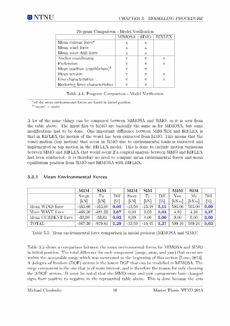
A lot of the same things can be compared between MIMOSA and SIMO, as it is seen fromthe table above. The input �les to SIMO are basically the same as for MIMOSA, but somemodi�cations had to be done. One important di�erence between MIM/SIM and RIFLEX isthat in RIFLEX the motion of the vessel has been extracted from SIMO. This means that thevessel motion (top motion) that occur in SIMO due to environmental loads is extracted andimplemented as top motion in the RIFLEX model. This is done to exclude motion variationsbetween SIMO and RIFLEX that would occur if a coupled analysis between SIMO and RIFLEXhad been conducted. It is therefore no need to compare mean environmental forces and meanequilibrium position from SIMO and MIMOSA with RIFLEX.

3.3.1 Mean Environmental Forces

MIM SIM MIM SIM MIM SIM

Surge Fx Di� Sway Fy Di� Yaw Mz Di�[kN] [kN] [%] [kN] [kN] [%] [kNm] [kNm] [%]

Mean WIND force -465,80 -465,80 0,00 -13,50 -13,48 0,15 505,00 505,00 0,00

Mean WAVE force -468,50 -481,00 2,67 0,00 0,03 0,03 4,10 4,24 3,37

Mean CURRENT force -33,00 -33,01 0,03 0,00 0,00 0,00 0,00 0,00 0,00

TOTAL -967,30 -979,81 1,29 -13,50 -16,45 0,37 509,10 509,24 0,03

Table 3.5: Mean environmental force comparison in initial position (MIMOSA and SIMO)

Table 3.5 shows a comparison between the mean environmental forces for MIMOSA and SIMOin initial position. The total di�erence for each component (surge, sway, and yaw) that occur arewithin the acceptable range which was mentioned in the beginning of this section [Lone, 2013].A 3-degree of freedom (DOF) system is the lowest DOF that can be modelled in MIMOSA. Thesurge component is the one that is of main interest, and is therefore the reason for only choosingthe 3-DOF system. It must be noted that the SIMO sway and yaw components have changedsigns from positive to negative in the represented table above. This is done because the axis



system are de�ned di�erently in MIMOSA and SIMO, and it is simpler to compare results whenthey have the same sign.

The surge components from the table above are now illustrated in a bar plot. It can now be seenmore clearly that the mean wave force is slightly larger in SIMO then in MIMOSA.

Figure 3.4: Comparing mean forces for surge component

3.3.2 Anchor Coordinates and Pretension

MIMOSA SIMO

Xglobal Yglobal Xglobal YglobalLine no. [m] [m] [m] [m]

1 1279,31 0,00 1279,31 0,00

2 1107,92 639,66 1107,92 -639,66

3 639,66 1107,92 639,66 -1107,92

4 0,00 1279,31 0,00 -1279,92

5 -639,66 1107,92 -639,66 -1107,92

6 -1107,92 639,66 -1107,92 -639,66

7 -1279,31 0,00 -1279,31 0,00

8 -1107,92 -639,66 -1107,92 639,66

9 -639,66 -1107,92 -639,66 1107,92

10 0,00 -1279,31 0,00 1279,31

11 639,66 -1107,92 639,66 1107,92

12 1107,92 -639,66 1107,92 639,66

Table 3.6: Comparing calculated anchor coordinates

Because the axis systems are de�ned di�erently in MIMOSA and SIMO it is seen from table3.6 that the Yglobal in SIMO have di�erent sign then for MIMOSA. Other than that, there is



no di�erence in the calculated anchor coordinates. MIMOSA and SIMO calculate the anchorcoordinates given the pretension, meanwhile RIFLEX calculates the pretension given the anchorcoordinates. So, to get the same pretension in RIFLEX the anchor coordinates have to be slightlychanged, see table 3.7. As mentioned previously, the main focus is on the windward and leewardlines (line 1 and 7) and in RIFLEX only these two lines have been modelled.

Anchor coor. PretsnionProgram [m] [kN]

MIM 1279,31 1000

SIM 1279,31 1000

RIF-1 1279,31 984,8

RIF-2 1279,52 1000

Table 3.7: Anchor coordinates and Pretension

To get the same pretension in RIFLEX the anchor coordinates in x-direction have to be change by±0,21m depending on if it is the leeward or windward line. The di�erence in anchor coordinatesis only 0,016%, which is relatively small and within acceptable range.

3.3.3 "Mean" Position (equilibrium)

Mooring position in global x-axis: 60,00m

MIMOSA SIMO Di�

X [m] Y [m] Yaw [deg] X [m] Y [m] Yaw [deg] [%] [%] [%]

Eq. position -62,20 -0,06 0,04 -62,03 0,03 -0,02 - - -

Changein turret pos. -2,20 -0,03 0,04 -2,03 0,03 -0,02 7,73 0,00 50,00

Table 3.8: "Mean" Position (equilibrium) comparison

Table 3.8 shows that there are di�erences in the calculated equilibrium position, notably inthe surge (x-direction). The di�erence in yaw is negligible since the values are small. In theconclusion at the end of this section the di�erence in the surge component will be investigatedmore thoroughly since the deviation is larger then 5%.



3.3.4 "Mean" tension

MIMOSA SIMO Di� Di�Line no. [kN] [kN] [kN] [%]

1 1180,10 1180,00 0,10 0,01

2 1153,70 1150,00 3,70 0,32

3 1084,90 1080,00 4,90 0,45

4 999,90 1000,00 -0,10 0,01

5 925,10 930,00 -4,90 0,53

6 876,80 877,00 -0,20 0,02

7 859,00 860,00 -1,00 0,12

8 875,20 875,00 0,20 0,02

9 922,30 928,00 -5,70 0,62

10 996,10 999,00 -2,90 0,29

11 1081,30 1080,00 1,30 0,12

12 1151,30 1150,00 1,30 0,11

Table 3.9: "Mean" Tension comparison

From table 3.9 we see that all the static ("mean") tension forces deviate less then 1%, which isquite good and acceptable.

3.3.5 Line Characteristics

(a) Original (b) Enlarged

Figure 3.5: Line characteristics for MIMOSA, SIMO, and RIFLEX (line 1). Negative x-value:moving towards the anchor. Positive x-value: moving from the anchor.



The two graphs above show that the line characteristics for the three programs; MIMOSA, SIMO,and RIFLEX follow each other quite well. The line characteristics in MIMOSA and SIMO areidentical, but deviate slightly from RIFLEX. These small di�erences are acceptable due to therule of thumb criteria mentioned in the beginning of this section. We can also see that thepretension (in X = 0, 00) is equal for all the programs due to the modi�cation made to theanchor coordinates in RIFLEX. Since all the mooring lines are identical, and we only need tolook at the line characteristics for one mooring line, see �gure 3.5.

3.3.6 Restoring Force Characteristics

Forcing the vessel in surge direction and stepwise �nding the resistance in mooring line 1, wecan obtain the restoring force characteristics for the line. The di�erences between MIMOSA andSIMO are within 5% as it can be seen from the �gure and table below.

Figure 3.6: Restoring Force Characteristics for MIMOSA and SIMO plotted from 0 to 2,50 m

O�set MIMOSA SIMO Di�[m] [kN] [kN] [%]

0,00 0,00 0,00 0,00 %1,50 -655,80 -651,10 0,72 %3,00 -1332,20 -1328,60 0,27 %4,50 -2047,00 -2050,20 0,16 %6,00 -2826,10 -2824,10 0,07 %7,50 -3693,80 -3685,70 0,22 %9,00 -4671,30 -4668,20 0,07 %10,50 -5791,80 -5793,00 0,02 %12,00 -7086,90 -7088,60 0,02 %13,50 -8574,20 -8566,20 0,09 %15,00 -10280,70 -10285,20 0,04 %

Table 3.10: Restoring force comparison between MIMOSA and SIMO



3.3.7 Conclusion - Model veri�cation

Comparing the static results for all models was done early in the modelling procedure, and it isimportant for further analysis. A conclusion table is made to illustrate, and to summarize thedi�erent comparisons that have been done in the process of verifying the di�erent models.

MIMOSA SIMO RIXLEX

Mean current force x x√

Mean wind force x x√

Mean wave drift force x x√

Anchor coordinates x x x√

Pretension x x x√

"Mean" position (equilibrium) x x√

"Mean" tension x x x√

Line characteristics x x x√

Restoring force characteristics x x√

Table 3.11: Conclusion table - Model Veri�cation

√- within acceptable range√- some modi�cations had to be made (mainly in RIFLEX). May a�ect the �nal result√- exceeds the acceptable range, need to be clari�ed

The mean equilibrium position exceeds the acceptable range when comparing MIMOSA andSIMO, and needs to be investigated. The di�erence in mean equilibrium position is becauseSIMO does not obtain static equilibrium throughout the iteration process. This can be seenfrom the SIMO result �le for static analysis, which is found on the attached CD (see appendixG). SIMO stops looking for the mean equilibrium position when a satisfactory error limit isreached. The residual force in surge for SIMO is -74.08 kN, while in MIMOSA the equilibriumposition is found. By simple hand calculations we can check what the actual di�erence in meanequilibrium position is suppose to be. We know that mooring line sti�ness can be found by:

k =∆F

∆x. (3.1)

By using the restoring force table (table 3.10) and �nding the mooring line sti�ness around themean equilibrium position (between 1,50 - 3,00 meters) the sti�ness for MIMOSA and SIMOthen becomes,

kMIM =1332, 20kN − 655, 80kN

3, 00m− 1, 50m= 450, 93

kN

m, (3.2)

kSIM =1328, 60kN − 651, 10kN

3, 00m− 1, 50m= 451, 67

kN

m. (3.3)

The di�erence in sti�ness is only 0.16 % and they are considered to be relatively equal. Bydividing the static residual force with the calculated sti�ness for SIMO, the residual static o�setbecomes:



xresidual =Fresidual

kSIM=

74, 08kN

451, 67kNm

= 0, 164m. (3.4)

The residual static o�set (xresidual) is almost the same as the di�erence in mean equilibriumposition (0,17m) between MIMOSA and SIMO (see table 3.8). This means that the di�erencearises because of the residual static force from SIMO, which occurs because SIMO does notobtain the exact mean equilibrium position.


Chapter 4

Program Structure

MIMOSA, SIMO, and RIFLEX are the programs used in this master thesis. As mentioned inthe previous chapter, SIMO and RIFLEX can be used in SIMA. The graphical interface in SIMAmakes it easy to use and it is much simpler to visualize the model. A choice was made quiteearly in the master thesis to also run all the programs in batch mode. This was done because allthe input �les had to be created and read, and one then gets full control over the whole analysisprocess. It was also simpler to interpret the error messages when using the programs in batchmode. Another reason for creating individual scripts for each program and then combining themwith one batch script was to make everything automatic. Typing in all the necessary �les for eachprogram, for every analysis is quite time consuming. So, by spending some time on creating onebatch �le that combines every single batch �le for all the individual programs was time savingin the long term.

Appendix G gives a description of structure and content of the attached CD. On that CD allthe �les used and created can be found. In appendix G there is also a table explaining all thedi�erent �le types that were created and used.

4.1 MIMOSA, SIMO, RIFLEX (MSR) Script - Main batch script

By creating a small batch script that was the called MSR program, was quite time saving in thelong run. All the individual programs; MIMOSA, SIMO, and RIFLEX could then be executedat the same time, or individually depending on the users choice. This combined script was usefulwhen the turret position was changed in the parameter study (section 3.2), and all the programsneeded to be executed once again. The �oat diagram below illustrates how the MSR scriptworks. Note that in the �oat diagram the MSR script is called MSR Program.

23

CHAPTER 4. PROGRAM STRUCTURE

Figure 4.1: Float diagram with description for MIMOSA, SIMO, RIFLEX (MSR) Script

Figure 4.1 shows how all the batch scripts are combined together, and the continuity of everysub-batch script will be shown later on with �oat diagrams of there own.

4.2 MIMOSA

The �oat diagram below shows how di�erent scripts within MIMOSA are coupled together forrunning multiple analysis, i.e. FEM-WF, QS-WF, and QS-LF. Figure 4.2 describes the di�erentcolors and arrows, and all the self made scripts can be found on the attached CD (see appendixG). The MIMOSA user's manual has been used as help for creating the MIMOSA scripts androutines [MIM, 2012].

Figure 4.2: MIMOSA script description



Figure 4.3: MIMOSA �oat diagram - script procedure

4.3 SIMO

The SIMO user's manual has been used as help for creating the scripts and routines in SIMO,[SIM, 2012b].

SIMO was used in SIMA and in batch mode. This following section will only go through theSIMO script in batch mode. SIMO is similar to MIMOSA in many ways, and here one couldalso create routines within the program and coupling them together with a batch script. Thescripts structure and coupling is visually explained in the �oat diagram below.



Figure 4.4: SIMO script description

Figure 4.5: SIMO �oat diagram - script procedure



4.4 RIFLEX

RIFLEX has a totally di�erent interface then SIMO and MIMOSA, and needs to be dealt withdi�erently. A batch script was made to run the di�erent modules automatically as it can be seenfrom the �oat diagram below. The RIFLEX user's manual was frequently used when creatingthe input �les for all the modules used in RIFLEX, [RIF, 2012b].

Figure 4.6: RIFLEX script description

Figure 4.7: RIFLEX �oat diagram - script procedure



4.5 Post Processing - Matlab

This Matlab script was made for processing the results given from MIM, SIM, and RIF. Thecoding can be found in appendix E, and on the attached CD (see appendix G).

Figure 4.8: Matlab script description

Figure 4.9: Matlab �oat diagram - script procedure

Note that every �le and every script can be found on the attached CD, and it is recommended toread through appendix G before accessing the CD. The post-processing scripts will be referredto a lot throughout this master thesis and is therefore included in appendix E.


Chapter 5

Program Theory

Several programs exist that can perform mooring line analysis. MIMOSA, SIMO and RIFLEXare all developed by MARINTEK and are the main programs that will be used for this masterthesis. Ariane and DeepC are examples of other programs that also can be used for analysingmoored systems. When using a computation program one must be aware of how the programworks. Every program has some advantages and disadvantages, and to have knowledge aboutthis will provide good reliable results and discussions. This chapter will cover a small amountof general theory for each program being used in this master thesis, and the main focus will beon how the di�erent programs calculate the standard deviation of tension forces in the mooringlines. The reasoning for mainly looking at STD of tension forces is discussed in section 2.3.

Mooring line response can be calculated in the frequency domain (MIMOSA) or in the timedomain (SIMO and RIFLEX). The following table summarizes the advantages, and disadvantagesbetween performing a frequency and time domain analysis. [Lone, 2009]

Frequency domain (FD) Time Domain (TD)

Advantages

Calculations are fast. Non-linearities are accounted for.No loss of statistical properties

Disadvantages

Non-linear systems are linearised For strong non-linear system many simulation are required.Only steady-state response Time-demanding

Program

MIMOSA SIMO and RIFLEX

Table 5.1: Advantages and disadvantages regarding the use of FD or TD methods

The three programs that are used can all model a 6-DOF system. Note that for this masterthesis only a 3-DOF system is modelled in MIMOSA, mainly because the surge motion is ofinterest and because the e�ects we are after appear for this motion.

29

CHAPTER 5. PROGRAM THEORY

5.1 MIMOSA

The content for this section is based on the MIMOSA course given by MARINTEK [Kaasen, 2012]and the MIMOSA User's manual [MIM, 2012]. Karl E. Kaasen has also been helpful withclarifying unclear subjects within the MIMOSA theory section [Kaasen, 2013].

Throughout this section we denote r as the projection of the horizontal distance from anchor totop end (farilead) of the line.

5.1.1 LF tension - Only Quasi-Statically

Two options are available for computing the LF tension:

1. A linearised model, which is non-Rayleigh based method developed by Carl Trygve Stans-berg,

2. Rayleigh based method.

The procedure for calculating LF tension is only done quasi-statically. It can be seen from theequation below, that the STD of LF tension is computed by using the LF vessel motion. LFmotions are computed with linearised models if option 1 is chosen from the list above. If we nowdenote rs as the static position of the mooring line, the STD of LF tension is in MIMOSA foundby:

σLFT = T (rs + σLFr )− T (rs). (5.1)

σLFT - STD of LF tension,

rs - static position, or mean o�set,

σLFr - STD of LF o�set (computed from response spectrum).

The interpretation of equation 5.1 is that MIMOSA uses the static position and the STD ofLF o�set directly in the line characteristics to �nd the STD of LF tension. If the mooring linecharacteristics is non-linear, MIMOSA will choose the value which obtains the largest STD ofLF tension. The next �gure illustrates this by showing that T-STD 1 is smaller then T-STD 2for the the same STD of LF o�set.



Figure 5.1: Calculating the STD of LF tension using mooring line characteristics, where T-STDis STD of tension

It is written in the MIMOSA user's manual that the STD of WF and LF tension calculationsare not true standard deviations, unless the displacement-tension characteristics are linear. Thismeans that if the mooring line characteristics curve in �gure 5.1 was linear, T-STD 1 and T-STD 2 would be equal and therefore would represent the true STD of LF tension. This indicatesthat for non-linear line characteristics there is a certain inaccuracy in the computed STD of LFtension.

5.1.2 WF tension - General

In MIMOSA there are three options for calculating the WF tension.

1. Quasi-static (QS) method

2. Simpli�ed Analytic Method (SAM)

3. Finite Element Method (FEM)

The SAM method will not be handled in this master thesis and the theory behind this calculationmethod is therefore not included. QS and FEM both use the base o�set, rb, when computing theSTD of WF tension for combined WF and LF motions. The base o�set is computed individuallyfor every line as a projection of the fairlead motion in the line plane (xz-plane). STD of WFand LF tensions are for this master thesis computed separately, and the use of base o�set isincluded here to show that there are di�erences in performing a separate and combined analysisfor obtaining the STD of WF tension.



rb =

{rs + rLFextr + (2σWF

r − rWFextr), r1 < r2

rs + 2σLFr , r1 ≥ r2(5.2)

where r1 and r2 are found by:

r1 =(2σLFr + rWFextr), (5.3a)

r2 =(rLFextr + 2σWFr ). (5.3b)

rLFextr - Extreme LF response (based on Rayleigh assumptions),

σWFr - STD of WF response (response spectrum),

rWFextr - Extreme WF response (based on Rayleigh assumptions),

σLFr - STD of LF response (response spectrum).

5.1.3 WF tension - QS

Inertia and damping forces are neglected when using the QS-method. As previously described,there is a di�erence between a separate (WF only) and coupled (WF&LF) analysis. This sectiondescribes the procedure for WF only.

This method uses the mean o�set (not the base o�set) and adding the STD of WF positiondirectly in the mooring line characteristics in obtaining the STD of WF tension. Drag forcesand other non-linearities acting on the line are not accounted for, but current forces acting onthe cable can be included in a simpli�ed manner. The STD of WF tension for the QS-method isfound similarly as for the STD of LF tension:

σWFT = T (rs + σWF

r )− T (rs). (5.4)

5.1.4 WF tension - FEM

The FEM accounts for inertia and drag forces. Current forces can be included in the samemanner as for the QS-method. In this computation method there is a procedure that accountsfor non-linearities. The aim is to �nd a estimate of dynamic WF tension. The mooring cable isnow modelled as multi-degree-of-freedom dynamical system and solved in the FD:

M∆�r+C∆r+K∆r = K0rWF + F (5.5)

∆r - Contains nodal displacement in (x,y,z) from the mean o�set, rs,

K - builds up a sti�ness matrix based on the line con�guration dependent on rs,

K0rWF - a given force from the WF motion at fairlead, where the motion (rWF ) is found fromthe response spectrum,

M - mass and added mass matrix are constant,



C - average linear damping coe�cient. Stochastic linearisation of the displacements at everynode. Creates coe�cients for every node. Iteration process in �nding the drag forces actingon every node is included in the damping coe�cient,

F - wave force vector that acts on the mooring line.

This method can also perform a separate and coupled analysis as for the QS-method, but here weonly have considered a separate analysis meaning that WF only has been used. The di�erencewould be that for the separate analysis, in our case WF only, the mean o�set is used. While forthe combined analysis the base o�set is used.

∆r will now be used in computing the STD of WF tension, σWFT , using the FEM. The FEM

model can only be used for long-crested waves because short-crested waves are not implementedin the MIMOSA program.

5.1.5 Non-linear WF tension - FEM

MIMOSA has a procedure that attempts to capture the e�ect of the non-linear nature of thedynamic cable model. This method is based on the assumption that the response spectrum isnarrow banded. The procedure for including the non-linear e�ects are as following:

1. σWFT will be found by the procedure described in the previous section.

2. MIMOSA �nds the max tension (Tmax) form Rayleigh calculations, and assumes that closeto the max tension top the amplitudes around this top are of equal magnitude.

3. Finds R =Tmax

σWFT

, which is a constant relationship between max tension and STD of WF

tension.

4. From point 2 MIMOSA then assumes a stationary sinusoidal response curve around theextreme top (Tmax). Because of this stationary sinusoidal assumption, the relationship

between σWFr and Tmax becomes; σWF

r =Tmax√

2.

5. The wave spectrum will now be scaled up by 0, 5R2 so that the amplitude between thestationary sinusoidal response curve and the calculated Rayleigh max value (Tmax) are ofequal magnitude. A new response including the non-linear e�ects will now be calculated

once again; σ̂WFr =

1√2∗R ∗ σWF

r .

6. This new calculated σ̂WFr will be multiplied by

√2 because of the sinusoidal response curve

assumption. The iteration process for solving eq.5.5 will be repeated, but now the σWFr

is replaced by σ̂WFr . σ̂WF

T will now be the new STD of WF tension including non-lineare�ects.

In the new iteration process (point 6) MIMOSA will �nd a new damping coe�cient to account forthe new drag forces, while the mass and sti�ness matrix will remain unchanged. The linearisedsti�ness matrix is kept constant and the touch down point is �xed at the sea-�oor. Retainingthe touch-down point is done so by �tting a hinge pin at this node [Leira, 2013].

There was some confusions around the usage of non-Rayleigh and Rayleigh based method, and ifthis would a�ect the STD of WF tension calculations. This issue was clari�ed by conversations



with Karl Kaasen [Kaasen, 2013]. The STD is an average measurement and will not be a�ectedby the choice of non-Rayleigh or Rayleigh method. On the other hand, the max tension valuewill depend on the choice of method.

5.2 SIMO

The content of this section is taken from SIMO theory and user's manual [SIM, 2012a], [SIM, 2012b].

SIMO uses a similar calculation procedure as MIMOSA for analysing mooring lines, and in SIMOthere are two methods which can be used:

1. Quasi static (QS) analysis

2. Simpli�ed dynamic analysis (SAM)

5.2.1 Mooring line tension

SIMO performs the analysis in the TD, and every mooring line is handled separately. Friction atthe bottom is neglected and the line can rotate freely about the anchor. For the QS method thetransverse drag on the lines are neglected. The procedure for calculating the total line tensionis similar as for MIMOSA, and the top tension is determined by the location of the upper endrelative to the anchor. This is done in a two dimensional plane (vertical plane/xz-plane).

The QS method uses the mooring line characteristics to �nd the line tension at the top end.In doing so SIMO uses a quadratic interpolation function to obtain the tension through thetime simulation [Mo, 2013]. This interpolation method will now be denoted as updated line

characteristics. The updated line characteristics means that geometrical sti�ness will be properlyaccounted for. The geometrical sti�ness is linearised in MIMOSA.

The SAM method that is available in SIMO accounts for dynamic e�ects in a simpli�ed way. Amethod that considers these e�ect has been developed by Larsen and Sandvik [Larsen and Sandvik, 1990].This simpli�ed method does not account for mass forces on the line, and is therefore a methodwhich only includes transverse drag forces.

Current forces acting on the mooring lines are not included in the QS and SAM in the SIMOprogram.

5.3 RIFLEX

The content for this section is taken from the RIFLEX theory and user's manual [RIF, 2012a],[RIF, 2012b].

RIFLEX was originally created for analysing �exible risers and other slender structures. RIFLEXis fully capable of conducting analysis of mooring lines in the TD. The general dynamic equilib-rium equation that RILFEX solves for dynamic TD analysis is:

RI(r,�r, t) +RD(r, r, t) +RS(r, t) = RE(r, r, t) (5.6)



RI - inertia force vector,

RD - damping force vector,

RS - internal structural reaction force vector,

RE - external force vector,

r, r,�r - structural displacement, velocity and acceleration vectors.

Eq. 5.6 is solved by step-by-step numerical time integration with equilibrium iteration at eachtime step. Available analysis methods in RIFLEX are:

1. Fully non-linear analysis,

2. Linearised FEM analysis.

The most important non-linear e�ects that have to be considered in a dynamic analysis are: (i)geometrical sti�ness of mooring line, and (ii) contact problems. Other types of non-linear e�ectscan be found in T. Moan's booklet given in the advanced �nite element course [Moan, 2003].Since this master thesis handles mooring lines the two listed e�ects above are the most importantnon-linear e�ects.

Contact problems are modelled as springs at the seabed. Geometrical sti�ness depends on themooring line con�guration. For slack mooring lines the non-linear geometry need to be properlyaccounted for. For both these computation methods, current forces acting on the mooring linescan be included.

5.3.1 Fully non-linear analysis

A fully non-linear analysis handles all non linearities properly and is rather time consumingcompared to MIM-FEM and SIM-QS method. This is because a fully non-linear analysis inRIFLEX establishes system matrices (mass, damping and sti�ness) repeatedly. Drag, currentand inertia forces acting on the mooring lines are accounted for. This method account for allthe desired e�ects with we are after, and this method is therefore considered to give the mostaccurate results.

5.3.2 Linearised FEM analysis

Linearised TD analysis is much less time consuming then a fully non-linear TD analysis. The step-by-step time integration now linearises the mass, damping and sti�ness matrix. These matricesare kept constant throughout the analysis. Keeping the sti�ness matrix constant means that thismethod linearises the geometrical sti�ness, and will not have a updated line characteristics whichis the case for the fully non-linear analysis. Non-linear hydrodynamics are accounted for whichmakes this linear analysis appealing when non-linear hydrodynamic e�ects are governing.



5.4 Summary of program theory

Table 5.2 summarizes what kind of non-linear dynamic e�ects are accounted for in the di�erentcomputations methods within MIMOSA, SIMO, and RIFLEX.

Method Updated . Current Drag andline char loads inertia loads

MIMOSA-QS - s -MIMOSA-FEM - s s

SIMO-QS√

- -SIMO-SAM

√- s

RIFLEX-linear -√ √

RIFLEX-Nonlinear√ √ √

Table 5.2: Compares di�erent e�ects that are included or not included in the calculation methodsfor all the three computation programs used. '

√' - accounted for in the analysis method. 's' -

accounted for in a simpli�ed manner.


Chapter 6

Case Study

System description, environmental loads that have been used throughout this master thesis willin this chapter be dealt with properly. The main goal is to �nd the di�erences between the threeprograms; MIMOSA, SIMO and RIFLEX that are of importance for fatigue damage analysis.These results are presented and discussed in chapter 7. The procedure in �nding these resultshave somewhat been covered in earlier chapters, meanwhile here some speci�c details are reviewedin how the results were found such as �lter design and calculation methods used within the threeprograms.

6.1 System Description

The case is a turret moored FPSO vessel at 100 m water depth. Table 6.1 presents the data forthe Aasgard FPSO T900s which was used throughout this master thesis.

FPSO DATA

Variable Value Unit Comment

T (draught) 16,50 m "medium" loading conditionLpp 258,00 m Distance from Ap to FpLpp/2 129,00 mLCG 113,58 m In front of ApRAO reference point 117,12 mRAO ref. - LCG 3,54 m Distance from LCG to RAO ref. point

Table 6.1: FPSO data given by Erling Lone, DNV

In chapter 3.2 we discussed the reason for modifying the original model to enhance the �nalresults. Reducing the pretension in the mooring lines and positioning the turret further awayfrom the COG (positive x-direction), were the only two changes made to the original model. Thetable below shows a column with the original data and one column with the modi�cations madeto the original model.

37

CHAPTER 6. CASE STUDY

Mooring System

Description Original Value Modi�ed Value Unit

Distance from COG to turret center 48,32 60,00 mVertical position of fairlead 15,97 15,97 mNumber of lines 12 12 [-]Segments per line 3 3 [-]Pretension (all lines) 1200 1000 kN

Table 6.2: Original and modi�ed mooring system data

The model consists of 12 identical mooring lines (for MIMOSA and SIMO) numbered in aclockwise direction, beginning with the one pointing towards north (see �gure 3.3). In RIFLEXonly the windward and leeward line have been modelled. Each mooring line consist of 3 segments,which were originally divided like shown in �gure 6.1.

Figure 6.1: Original mooring line composition

In the modelling process we found that the mooring system was to heavy and gave to muchsti�ness to the system [Lone, 2013], so the chain segment was changed to steel wire rope. Onesegment could just as well be modelled for the whole line, but since the modelling processwas well under way the three segment were kept, even though all the segments have the sameproperties.

Line Segment Properties

Segment no a Diameter Length No. of elements CD CL Type[m] [m] [m] [-] [-]

1 0,13 1050 70 2,40 1,15 Wire2 0,13 200 20 2,40 1,15 Wire3 0,13 50 10 2,40 1,15 Wire

Table 6.3: Line segment properties given by Erling Lone, DNV

aNumberd from anchor

Compared to general mooring systems, the system used here is still a sti� system even thoughmeasures have been made to make this particular mooring system less sti� [Lone, 2013].



The models for all the computation programs are restricted against rotations in yaw. This isdone because the surge motion will give rise to the largest tension forces in the mooring lines[Faltinsen, 1990]. This restricting is obtained by introducing an arti�cial sti�ness in the yawmotion.

6.2 Environmental Condition

As mentioned throughout this whole master thesis, it is important that every model is exposedto the same environment. Wind, waves and current are propagating towards south (from north),and the windward line is line 1 and leeward line is line 7.

Environmental Condition for MIMOSA, SIMO, RIFLEXa

Waves: HS = 8, 0m, TP = 12, 5s. Double Peaked Spectrum.Wind velocity: 20 m/s, 1 hour average 10m above surface. ISO 19901-1 (NPD) spectrum.Current velocity: 0,60 m/s at the surface.

Table 6.4: Environment description. Used for all models

aPrescribed motion from SIMO

In the RIFLEX model there is no actual environment that act on the model since RIFLEX hasa prescribed vessel motion from SIMO. This is for instance the reason for not checking the meanenvironmental forces from MIMOSA and SIMO with RIFLEX in section 3.3.

6.3 Calculation Methods

The MIMOSA, SIMO and RIFLEX theory manuals are used for this section [MIM, 2012],[SIM, 2012a], [RIF, 2012a].

6.3.1 General

The FD calculations for obtaining the STD of WF tension are performed in MIMOSA by theQS and FEM. A simpli�ed method (SAM) is also available but is not used in this master thesis.The FEM divides the cable in to elements, and the accuracy increases with increased number ofelements.

Current forces that act on the mooring lines can be included in the calculations in the MIMOSAprogram, but is disregard for all models. This is because SIMO is a program for motion sim-ulations and station keeping, and for a quasi-static analysis in SIMO the transverse drag forcecomponent is neglected and current is mainly included for calculating mean current forces andstatic o�set of the vessel. By neglecting the current forces acting on the mooring line we minim-ize the di�erences between the di�erent models, and this is acceptable since we are interested inother e�ects. Regarding or disregarding the current e�ects on the mooring lines will not in�uencethe line tension signi�cantly as it was described in section 2.1.1.



Body type 2 is chosen in SIMO, which means that the WF motions are pre-calculated in theFD, and LF motions are calculated in the TD throughout the whole simulation. By choosingthis body type in SIMO, the WF calculations will be more equal to the calculations done inMIMOSA because they use the same RAO's.

6.3.2 Time Domain

TD simulations are �rst performed in SIMO and prescribed vessel motions are then implementedin RIFLEX. RIFLEX then runs a TD analysis with the same simulation length as in SIMO. Thesimulation time was 9 hours and 300 seconds. The �rst 300 seconds of the simulation is removedbecause it takes some time before the simulation stabilizes, and 300 seconds were chosen justto be on the safe side. Usually, TD analysis are simulated for 3 hours. By running a 9 hoursimulation, statistical uncertainties are reduced.

For wave generation, Fast Fourier Transform (FFT) method was chosen. Cooley-Tukey Four-ier transform algorithm is used to pre-generate waves in SIMO. The FFT method is less timeconsuming then performing a simulation by summations of harmonic components for each timestep.

For TD analysis in SIMO and RIFLEX the Newmark− β procedure is used for numerical timeintegration, see [Langen and Sigbjôrnsson, 1999] for more detailed description of this method.The chosen parameters used for this procedure were:

γ = 0, 50 weighting parameter which gives no numerical dampingβ = 0, 25 weighting parameter which gives constant acceleration

(the trapezoidal method) that is unconditionally stable

SIMO: ∆t = 0, 5sRIFLEX: ∆t = 0, 5s Vessel motion (Irregular time series)

∆t = 0, 1s Line elements (Irregular response analysis)

6.4 Filter Design

When conducting a TD analysis in SIMO and RIFLEX the total tension force is calculatedfor the total duration of 9 hours. For analysing the WF and LF tension forces separately,�ltering the total tension result is necessary. Digital signal processing is a huge subject andsome basic knowledge is required for designing a good �lter. There is a lot of literature thatcan be found on digital signal processing, and the book written by Steven Smith [Smith, 1999]was particularly useful in this master thesis. Signal processing tools in Matlab include a lot ofdi�erent �lter models, and these �lters need to be tailored for �ltering WF and LF tension forces.The mathematics behind these �lters can be quite complex and will not be dealt with here. Onlythe terminology and the speci�c parameters are handled for creating a �lter that performs wellfor the desired purpose.

Filtering out the WF and LF tension forces requires a good �lter. A optimal �lter has:

� Good stop band attenuation

� Flat passband with small or none attenuation



� Fast roll-o�

In the process of designing a low and highpass �lter a FFT was performed on the total tensionforce time series for line 1 and 7. This was done to transform the tension forces from the TD tothe FD [Myrhaug, 2005], [Newland, 1993]. The following �gure shows the result of the FFT forthe time series in SIMO and RIFLEX. Built in Matlab function was used for performing an FFT,and the FFT procedure can be found in the Matlab code, appendix E (�lter_process.m).

Figure 6.2: FFT on the time series for SIMO (upper) and RIFLEX (lower) - line 1 (left) andline 7 (right)

From �gure 6.2 we see the tendency of a double peak spectrum. For line 7 (right) in both SIMOand RIFLEX the WF and LF peaks can clearly be seen. For the lowpass �lter we want to dampout all the high frequency contributions. So a cut-o� frequency was set to 0.03 Hz, which is aperiod of 33.33 s. The cut-o� point is the point between the LF and WF peaks, and this willnow became the basis for the designed �lter.

For minimum passband attenuation a Butterworth �lter was chosen. This �lter is based onChebyshev polynomials and the �lter order. After some attempts the optimal �lter order wasfound to be 4. As it will be shown later on, this order gave good �ltering performance and avoidedover�ow. As most �lter, also this �lter introduces a phase shift of the output signal relative tothe input signal. This was not corrected for because this will not have any in�uence on the �nalresult since the goal is to �nd the STD of WF and LF tension forces. The sampling frequency(Fs) was set to 2 Hz for SIMO and 10 Hz for RIFLEX, and this Fs must be equal the time stepgiven in the SIMO and RIFLEX analysis. Figure 6.3 shows the constructed Butterworth �lter



used for �ltering LF and WF tension forces from the total tension force time series.

Figure 6.3: Designed �lter. 4th order Butterworth bandpass �lter

After the �ltering process was done a simple test was performed to check if the designed �lterwas accurate enough. Since we have a double peaked spectrum and the fact that WF and LFtension forces are separable as seen from �gure 6.2, the total STD of tension forces for line 1 and7 can simply be calculated by using the �ltered STD of WF and LF tension forces:

σTOTFilter =√σ2LFFilter + σ2WFFilter (6.1)

The next table shows a comparison between the calculated total STD tension force (σTOTFilter)and the original un�ltered STD tension force (σTOTOriginal):

σTOTFilter σTOTOriginal Di�[kN] [kN] [%]

SIMO - ∆t = 0,5s = 2Hz

Line 1 187.38 188.27 0.47

Line 7 117.86 117.92 0.05

RIFLEX - ∆t = 0,1s = 10Hz

Line 1 192,69 193,61 0.47

Line 7 136.68 132,72 0.03

Table 6.5: Comparing calculated STD tension with the original STD tension force

The data for this table can be found in appendix E under section RESULTS.txt. From theseresults we see that the di�erence between the calculated total STD tension force (σTOTFilter)and the original un�ltered STD tension force (σTOTOriginal) deviate less then 0,50 % for bothlines. This basically means that the designed �lter is quite good, and can be used to �lter outthe LF and WF tension forces from the total tension force time series.

The next two �gures will show how the �ltered WF and LF tension forces corresponds to theoriginal tension forces, which include both WF and LF tensions (WF&LF). From these �guresit is seen that the �ltered tension forces are phase shifted. As mentioned previously this will nota�ect the results since we are interested in STD of WF and LF tension forces.



Figure 6.4: Original (WF&LF) and �ltered WF and LF tension forces for line 1 (upper) and line7 (lower) for SIMO

Figure 6.5: Original (WF&LF) and �ltered WF and LF tension forces for line 1 (upper) and line7 (lower) for RIFLEX



For illustrative purposes the time series is plotted from 300 s - 1300 s. From �gure 6.4 and 6.5 wesee that the �ltered WF and LF tension forces follow the original (WF&LF) tension series quitewell. For our case we have a pretension of 1000 kN, and it can be seen that the original tensionforces for line 1 (windward line) �uctuates between a mean tension above the set pretension. Theoriginal tension forces for line 7 (leeward line) does the same except that the mean tension valueis beneath the set pretension. This con�rms that the mooring lines behave as expected, meaningthat it is expected that line 1 is experiencing larger and line 7 is experiencing less tension forcesthen the set pretension.

6.5 Fatigue Analysis

A small fatigue analysis was carried out in this master thesis. This is done because it is interestingto show how the fatigue damage is a�ected for di�erent sea-states. Simpli�ed methods have beenused and will be explained in this section.

In an article written by C.M. Larsen [Larsen, 1987], he performed a long-term fatigue analysisof risers on a tension-leg platform (TLP). The conclusion from this article was that for extremesea-states, Hs larger then 10 m, can be neglected when it comes to fatigue damage because theprobability for this sea-state to occur is small. Inspired by this, a similar fatigue analysis wasperformed on the mooring lines to see what sea-states contribute to fatigue damage.

For calculating the fatigue damage, the same sea-states has been used as in the article, andthe combined spectrum (CS) approach was used for these calculations. The sea-states used canbe found in appendix F. The equations used can be found in section 2.3 or in the DNV rules,[DNV, 2010]. This small fatigue damage analysis is done just to illustrate how the STD WF andLF tensions can be used directly in the fatigue analysis.

Even though the calculation performed here are simpli�ed compared to the calculations donein the article, the same conclusion can be drawn here. Hs larger then 10 m will contributeminimally for the fatigue damage on line 1 and 7. Even though the maximum stresses are largefor Hs larger then 10 m the probability for this sea-state to occur is small. When conductingthe fatigue analysis only MIM-FEM was used. MIMOSA computes in the FD and is less timeconsuming then for instance conducting this analysis in SIMO or RIFLEX.



Figure 6.6: Fatigue damage graphs. Maximum stress line 1 (upper left), fatigue damage resultsusing CS approach (upper right). Maximum stress line 7 (lower left), fatigue damage resultsusing CS approach (lower right)

Note that by looking at the maximum stress curve for both cases, we see that the windwardline is dominated by LF motion, while leeward line is dominated by WF motion. This will bediscussed more thoroughly later on.


Chapter 7

Results and Discussions

It is important to keep in mind that the system which was described in the previous chapter andthen analysed, is a modi�ed system. These modi�cations are made to enlarge and isolate di�erente�ects that occur when analysing a turret moored FPSO. Even though it is not a completelyreal system these e�ect will be present for cases which are similar to the case used in this masterthesis, which was a turret moored FPSO in shallow waters.

7.1 Results

In the process of computing the results the following must be kept in mind:

� Separate analysis was carried out for all computation methods in MIMOSA (see section2.2), which means that WF only and LF only options have been used,

� wind, waves and current propagate in the same direction for MIMOSA and SIMO (towardssouth) hitting the vessels bow,

� current forces acting on the mooring lines are not included in the analysis,

� contact forces (friction) between the mooring lines and sea-�oor is also not included becauseall the programs; MIMOSA, SIMO, and RIFLEX model this di�erently,

� the vessel has restricted rotations in yaw (see section 6.1),

� static o�set is due to mean environmental loads acting on the �oating vessel for MIMOSAand SIMO while RILFEX has a prescribed motion from SIMO with the same static o�set(see section 3.3),

� in MIMOSA and SIMO all the mooring lines were modelled, while in RIFLEX only thewindward (line 1) and leeward line (line 7) were modelled (see chapter 3),

� �ltering was necessary to separate WF and LF tension forces for the time series simulationsperformed by SIMO and RIFLEX (see section 6.4),

� due to combined response spectrum the total STD tension in MIMOSA was calculated byusing STD of WF and LF tension. In section 6.4 we verify that this approach is acceptableto use,

46

CHAPTER 7. RESULTS AND DISCUSSIONS

� STD of WF and LF tension was calculated by using Matlab for SIMO and RIFLEX basedon �ltered TD tension series, while these were given results from the MIMOSA analysisoutput �le due to calculations made in the FD.

Abbreviation Description (*)= WF or LF

MIM_FEM_(*) MIMOSA: Computes STD of WF or LF tension using FEM.MIM_QS_(*) MIMOSA: Computes STD of WF or LF tension using the QS

method.

SIM_QS_(*) SIMO: Filtered and calculated STD of WF or LF tensionusing body type 2, QS method.

RIF_FEM_(*) RIFLEX: Filtered and calculated STD of WF or LF tensionfor a fully non-linear FEM analysis.

DIFF Percent di�erence between value 1 og value 2.A negative DIFF means that value 1 is smaller then value 2,while a positive DIFF means that value 2 is larger then value 1.

Ratio Ratio between value 1 and value 2.

Table 7.1: Description of calculation methods, explanation of abbreviations used in tables andgraphs. For a more detailed description of computation methods see chapter 5

Figure 7.1: Comparing the main results from MIMOSA, SIMO and RIFLEX in a barplot



LINE 7 - Leeward

Value 1 [kN] Value 2 [kN] DIFF Ratio

1 MIM_QS_WF 56,64 SIM_QS_WF 59,33 -4,75 % 0,952 SIM_QS_WF 59,33 RIF_FEM_WF 81,44 -37,27 % 0,733 MIM_QS_WF 56,64 RIF_FEM_WF 81,44 -43,79 % 0,704 MIM_QS_WF 56,64 MIM_FEM_WF 66,49 -17,39 % 0,855 MIM_FEM_WF 66,49 RIF_FEM_WF 81,44 -22,48 % 0,82

6 MIM_QS_LF 104,94 SIM_QS_LF 101,90 2,90 % 1,037 SIM_QS_LF 101,90 RIF_FEM_LF 104,80 -2,85 % 0,978 MIM_QS_LF 104,94 RIF_FEM_LF 104,80 0,13 % 1,009 MIM_QS_LF 104,94 MIM_FEM_LF 104,94 0,00 % 1,0010 MIM_FEM_LF 104,94 RIF_FEM_LF 104,80 0,13 % 1,00

LINE 1 - Windward

Value 1 [kN] Value 2 [kN] DIFF Ratio

1 MIM_QS_WF 35,61 SIM_QS_WF 37,87 -6,35 % 0,942 SIM_QS_WF 37,87 RIF_FEM_WF 40,61 -7,24 % 0,933 MIM_QS_WF 35,61 RIF_FEM_WF 40,61 -14,04 % 0,884 MIM_QS_WF 35,61 MIM_FEM_WF 34,81 2,25 % 1,025 MIM_FEM_WF 34,81 RIF_FEM_WF 40,61 -16,66 % 0,86

6 MIM_QS_LF 182,76 SIM_QS_LF 184,43 -0,91 % 0,997 SIM_QS_LF 184,43 RIF_FEM_LF 189,31 -2,65 % 0,978 MIM_QS_LF 182,76 RIF_FEM_LF 189,31 -3,58 % 0,979 MIM_QS_LF 182,76 MIM_FEM_LF 182,76 0,00 % 1,0010 MIM_FEM_LF 182,76 RIF_FEM_LF 189,31 -3,58 % 0,97

Table 7.2: Main comparison results for line 1 and 7. All the values in the table are STD, andthe table is sorted in the order of importance

In the table above the leeward line is presented �rst because this will be the main focus throughoutthe discussions. The windward line will be used to compare with the leeward line.

The �rst observation made is the di�erence in magnitude between LF tension for the windwardand leeward line. The LF tension for line 1 is almost twice as large as for line 7. This di�erencewill be discussed in the following section.

From table 7.2 and �gure 7.1 we see that the di�erence between the STD of LF tension deviateless then -4% for all values that are compared for both windward and leeward line. We also havea veri�cation that MIMOSA computes the STD of LF tension equally regardless of using QS orFEM (comparison 9 for both line 1 and 7), as was described in section 5.1.

For the windward line the largest observed di�erence for STD of WF tension is for comparison5, which is -16,66%.

For the STD of WF tension for the leeward line there are signi�cant di�erences observed forcomparison 2 to 5, and the largest di�erence is found for comparison 3 which is -43,79%.



7.2 Windward vs. Leeward line

For the windward line (line 1) we see that the total STD tension is dominated by STD ofLF tension, while the total STD tension for the leeward line (line 7) is dominated by STD ofWF tension. To explain these di�erences we need to look at the motion for a turret mooredFPSO.

Since the incoming environment propagate in the same direction, the motion of a turret mooredFPSO will be elliptical in the xz-plane [Lone, 2009]. This means that the resulting force actingon the windward line will be larger then for the leeward line, which can be seen from the results.A illustration is made to show the elliptical motion for the turret moored FPSO and the resultingforces due to this motion. Note that �gure 7.2 is a illustration so, resulting forces, depth and soon are not up to scale.

Figure 7.2: Illustration of a elliptical motion for a turret moored FPSO, and the resulting forcesdue to this motion (red arrows)



Figure 7.3: Comparing �ltered WF and LF tension forces for windward (line 1) and leeward line(line 7) from RFIELX time series. Plot: 300 s - 1300 s.

Figure 7.3 shows a plot from 300 s - 1300 s, and we can clearly see that the amplitudes for LFtension are larger for line 1 then for line 7. The opposite can be said for WF tension forceswhere the leeward line has larger WF tension contributions then the windward line. This trendcontinues throughout the whole 9 hour simulation. This was �rst observed in �gure 6.6 in section6.5.

Due to the elliptical motions for a turret moored FPSO, line 1 will be more tightened up, whileline 7 will have a more non-linear slack con�guration. Because line 1 is more taut, WF motionswill not in�uence the total motion as much as they will for line 7. The combined WF and LFmotions will therefore a�ect the total tension forces di�erently for the two mooring lines. Thiscan be seen from the main results and on �gure 7.3.



7.3 Comparison di�erences between methods: STD of WF ten-sion

Table 7.2 is the basis for the discussions throughout this section. The main focus will be on theSTD of WF tension for the leeward line since these comparison values deviate the most in themain results, and also because the leeward line is the critical line for fatigue damage.

The di�erence between MIM_FEM_WF and RIF_FEM_WF (comparison 5) for the leewardline is the main result which we are after. To be able to explain what causes the variation betweenthem we need to rule out di�erent e�ects with help from di�erent computation methods. This isthe reason for also performing the analysis in SIMO, and using these results to isolate di�erente�ects.

7.3.1 Importance of updated line characteristics

For comparison 1 (QS-method for MIM and SIM), the only di�erence between the computationmethods is that SIMO updates the line characteristics, as described in section 5.2. This meansthat the geometrical sti�ness is properly accounted for in SIMO. A di�erence of -4,75 % showsthat for a non-linear mooring line characteristic, this e�ect needs to be considered, and by usingthe QS-method in MIMOSA will not su�ciently handle this e�ect.

Comparing the comparison 1 di�erences between the leeward and windward line we see thatwindward line has a higher di�erence (-6,35%) in percent then for the leeward line (-4,75%).

The explanation of this di�erence for comparison 1 has to do with the non-linear mooring linecharacteristics. Let us now introduce a local axis system at the top end (fairled) of the mooringlines 1 and 7, respectfully. The x-axis for the two mooring lines will have opposite directions inthe global axis system which has a positive x-axis towards north. The system is in initial positionfor x = 0, 00m. When static equilibrium is found, about x = −2, 00m in global axis system,the local x-coordinate for the windward line will be the same (orientated towards north). Forthe leeward line, which has the x-axis in the other direction (towards south) in the global axissystem, the local x-coordinate will be x = 2, 00m.

This means that we will move further down for the windward line, and further up for the leewardline in the line characteristics. Since MIMOSA and SIMO has the same line characteristics, thewindward line will move to a area where the line characteristic is non-linear. The leeward linewill then move to a location where the line characteristic is less non-linear. Since MIMOSAuses a linearised interpolation method for �nding the STD of WF tension for the QS-method,the di�erence between MIMOSA and SIMO will be larger in a area where the line character-istics are more non-linear, and therefore the di�erence when comparing MIM_QS_WF withSIM_QS_WF for line 1 and 7.

If WF and LF combined (WF&LF) calculations had been carried out, then the STD of LFmotions would be included in the calculation of the STD of WF tension. The di�erence betweenthe methods used in comparison 1 would most likely be smaller. A suggestion for further workcan be to verify if this is true.



7.3.2 Importance of dynamic e�ects

When dynamic e�ects are mentioned it means that drag and inertia forces on the mooringlines are included and accounted for in the computation method. We now want to assess theimportance of dynamic e�ects on the windward and leeward lines.

The only di�erence between SIM-QS and RIF-FEM (comparison 2) is that the fully non-linearanalysis in RIFLEX accounts for dynamic e�ects. By comparing these to methods we un-doubtedly see that dynamic e�ects are of high importance for the leeward line. -37,27% dif-ference for the leeward line indicates that dynamic e�ects must be included in the analysis toget accurate results when calculating the STD of WF tension. When drag forces are included,we know that the WF tension response will be phase shifted [Faltinsen, 1990]. This can clearlybe seen from �gure 7.4 where RIF-WF is phase shifted compared to SIM-WF because RIFLEXaccounts for drag and inertia forces.

Figure 7.4: Comparing WF tension between SIMO and RIFLEX for leeward line (upper graph).Lower plot is the surge motion for the same time series. Plot: 300 s - 500 s

The windward line will on the other hand have less dynamic e�ects then the leeward line becausethis line is more taut. A di�erence of -7,24% is considerably less then for the leeward line. Thisis again a con�rmation that the leeward line experiences large dynamics, and is the critical linefor fatigue damage.



Comparison 3 is the di�erence between the MIM-QS and RIF-FEM. As previously discussedthe fully non-linear analysis in RIFLEX accounts for geometrical sti�ness and dynamic e�ects,see conclusion of program theory section 5.4. For MIM-QS non of these e�ects are accountedfor. One would then expect that the di�erence for this comparison would increase for both theleeward and windward line. From the results we see that this is also the case, because twoessential e�ects are not accounted for in MIM-QS: (i) updated line characteristics, (ii) dynamice�ects.

7.3.3 STD of WF tension: MIM-QS vs MIM-FEM

MIM-QS and MIM-FEM are both computation methods that calculated in the FD. MIM-FEM isthe method which uses a simpli�ed method to account for dynamic e�ects, see section 5.1. Thismeans that the di�erence of -17,39% for the leeward line in comparison 4 is mainly due to thesimpli�ed method for accounting dynamic e�ects in the MIM-FEM. Neither of these computationmethods account for updated line characteristics, so this will be the same for both as well as thestatic o�set.

The di�erence between comparison 3 and 4 is that RIF-FEM properly accounts for dynamice�ects and updated line characteristic. Since the di�erence between comparison 3 and 4 should,theoretically, be the updated line characteristics, one would expect a small percent di�erencebetween comparison 3 and 4. The actual di�erence between comparison 3 (-43,79%) and 4 (-17,39%) for the leeward line is over 50%, which is larger then one would expect. This meansthat there are other e�ects which cause this di�erence.

From the MIMOSA theory section, section 5.1, we found that MIM-FEM linearises the touch-down point, or in other words, keeps the bottom node �xed. We also know that MIM-FEMuses a simpli�ed method that accounts for dynamic e�ects. These two mentioned properties forMIM-FEM is what causes the di�erence in comparison 4. MIMOSA linearises all the non-lineare�ects. So for strongly non-linear e�ects, the linearisation of these e�ect may not be su�cientenough.

For the windward line the comparison di�erence is 2,25% (comparison 4), which is interesting. Itis not quite clear what causes the MIM-QS to over predict the STD of WF tension. One possibleexplanation for the di�erence could be the vertical line characteristics. Because of the vesselselliptical motion, the reality would be that one also needs to account for line characteristics whichvaries in vertical direction (z-direction). The line characteristics that have been used throughoutthis master thesis is only considered for horizontal displacements (x-direction), because our mainfocus has been on the surge motion which is the critical motion for fatigue damage.



7.3.4 STD of WF tension: MIM-FEM vs RIF-FEM

Comparison 5 is the main goal of this master thesis. The di�erence found here is the di�erencebetween a simpli�ed computation method in the FD, which computes quickly, and a fully non-linear TD analysis that uses signi�cantly more computation time.

Lets now recapitulate what we know for these two methods:

MIM-FEM - dynamic e�ects are found by a simpli�ed method

RIF-FEM - dynamic e�ects and updated line characteristic are properly accounted for

The main di�erence between these various methods should be the updated line characteristics.Because the di�erence is -22,47% there is a suspicion that the simpli�ed method for accountingdynamic e�ects in MIM-FEM is not su�cient enough. This suspicion arises because the di�erencein comparison 1, where the di�erence only is updated line characteristics, is much less then thedi�erence in comparison 5. This means that the simpli�ed method used to account for dynamice�ects in MIM-FEM contribute signi�cantly to the di�erence between MIM-FEM and RIF-FEM.

On the other hand, if we look at comparison 4 (MIM-QS and MIM-FEM) we see that dynamice�ects in MIMOSA give rise to a di�erence of -17,39%. When adding the updated line char-acteristics, which we get in comparison 5 (MIM-FEM and RIF-FEM), the percent di�erenceincrease to -22,47%. This increase is somewhat similar to the percent di�erence in comparison 1(MIM-QS and SIM-QS).

It is hard to point out exactly what causes the di�erence in comparison 5, but we can nowsay that it most de�nitely has something to do with the linearisation process used in the linecharacteristics and in the simpli�ed method used in accounting for dynamic e�ects in MIM-FEM.For mooring lines which are dominated by WF motion and has a non-linear con�guration, thedi�erences between MIM-FEM and RIF-FEM can be relatively large for turret moored FPSOin shallow waters. A table is made to summarize the di�erent e�ects which are included inthe di�erent computation methods. This table gives an overview of what has been discussedthroughout this chapter.

Method 1 vs. Method 2Di�erences between Di�.computation methods leeward

line

1 MIM_QS_WF SIM_QS_WF Updated line characteristic (SIM) -4,75 %

2 SIM_QS_WF RIF_FEM-WF Dynamic e�ects (RIF) -37,27 %

3 MIM_QS_WF RIF_FEM-WFUpdated line characteristic (RIF)

-43,79 %Dynamic e�ects (RIF)

4 MIM_QS_WF MIM_FEM_WF Dynamic e�ects simpli�ed (MIM_FEM) -17,39 %

5 MIM_FEM_WF RIF_FEM_WFDynamic e�ects (RIF)

-22,47 %Dynamic e�ects simpli�ed (MIM_FEM)Updated line characteristic (RIF)

Table 7.3: STD of WF tension di�erence for leeward line (line 7)


Chapter 8

Conclusion

8.1 Conclusion from discussions and results

A quote from guidance note on page 40 in the o�shore standard DNV-OS-E301, [DNV, 2010];

"Catenary moorings without buoyancy elements or clump weights will have a quasi static beha-

viour in shallow waters (water depths < 100m)"

It is seen from the results and discussions that simpli�ed methods computed in the FD givesatisfactory results for calculation the STD of LF tension. All the comparisons deviate lessthen -4% for both the windward and leeward line when comparing the calculations for STD LFtension. It is noted that some dynamic e�ects (drag and inertia forces) are present for both lines,and that the windward line deviate the most when MIM-FEM and RIF-FEM are compared. Aquasi-static representation for computing the STD of LF tension is acceptable for both mooinglines.

The leeward line has been the main focus throughout this master thesis mainly because thisline is dominated by WF motion and will therefore be the line which experience the largest linedynamics. The windward line was also modelled, and has been used to compare with the leewardline.

From the results and discussions one thing is quite clear, that dynamic e�ects and geometricalsti�ness needs to be properly accounted for, especially for the leeward line. When comparing theSTD of WF tension for SIMO QS method with RIFLEX fully non-linear analysis, both in timedomain, the di�erence was -37,27%. The di�erence here gives an indication of how important itis to account for dynamic e�ects. The comparison between MIMOSA and SIMOs QS methodshowed that to account for geometrical sti�ness, updated line characteristic is necessary.

For the turret moored FPSO analysed in this master thesis, a QS representation of the mooringlines is not recommended for the leeward and windward line because the STD of WF tensionwill be too conservative. The di�erence between the simpli�ed FEM in MIMOSA and thefully non-linear TD analysis in RIFLEX was -22,48% for the leeward line, and -16,66% forthe windward line. The di�erence here is mainly caused by the linearisation methods used inMIMOSA to account for geometrical sti�ness and dynamic e�ects (drag and inertia forces actingon the mooring line). Using the simpli�ed FEM in MIMOSA one will under predict the STD

55

CHAPTER 8. CONCLUSION

of WF tension for the windward and leeward line, and therefore under predict the results in theestimation of fatigue life in the mooring lines.

8.2 Suggestions for further work

It would be interesting to perform a study that varies the environmental conditions for this turretmoored FPSO, and to see what the di�erences in comparing the di�erent computation methodswould then be. It is obvious that for more calm sea-states the dynamic e�ect will decrease andperhaps not be of the same importance as shown in this study. Since our modi�ed system isrelatively sti�, it would also be interesting to see what would happen for a less sti� mooringsystem. By varying the mooring system properties for the same turret moored FPSO, and thencomparing these results with the once found for this master thesis would also be interesting.

Performing a parameter study where pretension and turret horizontal position is varied wouldalso be interesting. The interesting part here would be to see if the di�erences are of the samemagnitude as shown for this master thesis.

Current forces acting on the mooring lines and bottom friction is disregarded for all the analysisperformed in this master thesis. This was done because all the programs (MIM,SIM,RIF) modelthis di�erently, and to account for this would introduce more uncertainties in isolating the dif-ferent e�ects between computation methods. It would therefore be interesting to see, if currentforces and friction were included, how this would a�ect the comparison between MIM-FEM andRIF-FEM. A suggestion for including current forces on the mooring lines could be to includea linearly decreasing current pro�le. MIMOSA and RIFLEX can include current forces on themooring lines, while in SIMO this possibility is not included.

Even though a small fatigue analysis was carried out, a more thorough fatigue analysis based onthe results would be interesting. One could retrieve environmental data form a real location at a100 m water depth, and then use these data in a similar analysis as conducted in section 6.5. Itwould also be very interesting to perform a comparison study between fatigue damage methods,e.g. comparing Rain-Flow counting (RFC) with the Combined Spectrum (CS) approach.

Another suggestion for further work would be to conduct a study where the main focus is on thedi�erences in extreme value statistics for MIMOSA. This is because MIMOSA computes in theFD and uses extreme statistics to �nd max tension in the mooring lines. Conducting a studywhere the main focus is to see if there are any di�erences by running a Rayleigh or non-Rayleighbased analysis.

8.3 Practical improvement

Self made scripts can always be improved to reduce computation time. Even though the post-processing script made in Matlab only used 2 minutes, improvements can be done.

One practical improvement which could be done is to program everything in Matlab. Matlab canexecute batch commands, and one of the advantages in coding everything in Matlab would bethat the post-processing scripts and batch scripts would run simultaneously. In Matlab one couldalso create better de�ned directories for saving the analysis results for all programs. Because this


CHAPTER 8. CONCLUSION

knowledge of Matlabs capabilities of execution batch commands came at the end of this masterthesis, all the batch scripts created were kept.

Running di�erent environmental conditions would on the other hand cause some problems whenprogramming everything in Matlab. Matlab would have to create a new sys.dat �le for SIMOevery time the environmental conditions were changed, and to make a script that creates a newsys �le for every environment would be quite time consuming.

All in all, the script which were made and used served there purposes, and did so quite well.A small drawback would be that if some changes were made to the model, for instance turretposition, these changes needed to be done manually in the input �les. This could be donedi�erently by creating a script which creates input �les as mentioned earlier.


Bibliography

[DNV, 2010] (2010). DNV O�shore Standard, DNV-OS-E301 Position Mooring.

[MIM, 2012] (2012). MIMOSA User's Documentation, Program version 6.3-06. MARINTEK,Trondheim, Norway.

[RIF, 2012a] (2012a). RIFLEX Theory Manual Vertion 4.0 rev.0. MARINTEK, Trondheim,Norway.

[RIF, 2012b] (2012b). RIFLEX User's Manual Vertion 4.0 rev.3. MARINTEK, Trondheim,Norway.

[SIM, 2012a] (2012a). SIMO Theory Manual Version 4.0 rev.0. MARINTEK, Trondheim, Nor-way.

[SIM, 2012b] (2012b). SIMO User's Manual Version 4.0 rev.0. MARINTEK, Trondheim, Nor-way.

[Faltinsen, 1990] Faltinsen, O. (1990). Sea Loads on Ships and o�shore structures. CambridgeUniversity Press.

[Fylling and Larsen, 1982] Fylling, I. and Larsen, C. (1982). Dynamic behaviour of anchor lines.Norwegian Maritime Research, 3:18�32.

[Kaasen, 2012] Kaasen, K. E. (2012). Mimosa: Interactive static and dynamic mooring systemanalysis. MIMOSA Course, 17.09.2012, MARINTEK.

[Kaasen, 2013] Kaasen, K. E. (2013). 19.04.2013, Private communication.

[Langen and Sigbjôrnsson, 1999] Langen, I. and Sigbjôrnsson, R. (1999). Dynamic response ofmarine structures (tmr4305).

[Larsen, 1987] Larsen, C. (1987). Fatigue life analysis of production risers. In OTC 5468 O�shore

Thechnology Conference.

[Larsen and Sandvik, 1990] Larsen, K. and Sandvik, P. (1990). E�cient methods for the cal-culation of dynamic mooring line tension. Proceedings of the First (1990) European O�shore

Mechanics Symposium, ISOPE:482�489.

[Leira, 2013] Leira, B. (2013). 19.04.2013, Private communication.

[Lone, 2009] Lone, E. N. (2009). Stochastic analysis of anchor line forces for �oating productionunits. Master's thesis, Department of Marine Technology, NTNU.

[Lone, 2013] Lone, E. N. (2013). Private communication.

58

BIBLIOGRAPHY

[Miedema, 2013] Miedema, S. (2013). Turret mooring. http://www.offshoremoorings.org/

moorings/2006/Groep6/Real%20page/Turret_main.htm.

[Mo, 2013] Mo, K. (2013). 25.04.2013, Private communication.

[Moan, 2003] Moan, T. (2003). TMR4190 Finite Element Modelling and Analysis of Marine

Structures. Department of Marine Technology.

[Myrhaug, 2005] Myrhaug, D. (2005). TMR4235 Stochastic Theory Of Sealoads. Department ofMarine Technology.

[Newland, 1993] Newland, D. (1993). An introduction to random vibrations spectral and waveanalysis. Lecture Notes from TMR4235 Stochastic Theory of Sealoads by Dag Myrhaug.

[NTNU-Library, 2013] NTNU-Library (2013). http://www.ntnu.edu/ub.

[Ormberg et al., 1997] Ormberg, H., Fylling, I., Larsen, K., and Sødahl, N. (1997). Coupledanalysis of vessel motions and mooring and riser system dynamics. In Proceedings of the

International Conference on O�shore Mechanics and Arctic Engineering - OMAE, pp. 91-100.

[Ormberg and Larsen, 1998] Ormberg, H. and Larsen, K. (1998). Coupled analysis of �oatermotions and mooring dynamics for a turret-morred ship. Applied Ocean Research, 20:55�67.

[SMB-O�shore, 2013] SMB-O�shore (2013). Turret mooring systems. http://www.

sbmoffshore.com/what-we-do/our-products/turret-mooring-systems/.

[Smith, 1999] Smith, S. W. (1999). The Scientist and Engineer's Guide to Digital Signal Pro-

cessing. California Technical Publishing.

[Storller, 2012] Storller, R. (2012). 27.09.2012, Course in Information Retrieval.

[Webster, 1995] Webster, W. C. (1995). Mooring-induced damping. Ocean Engineering, 22:571�591.


http://www.offshoremoorings.org/moorings/2006/Groep6/Real%20page/Turret_main.htm

http://www.offshoremoorings.org/moorings/2006/Groep6/Real%20page/Turret_main.htm

http://www.ntnu.edu/ub

http://www.sbmoffshore.com/what-we-do/our-products/turret-mooring-systems/

http://www.sbmoffshore.com/what-we-do/our-products/turret-mooring-systems/

BIBLIOGRAPHY


Appendix A

Information Retrieval

When writing a scienti�c article, or a master thesis it is important to use information with goodquality and that has been approved by scientists within the �eld of your study. What kind ofdatabases that have been used is important to ensure that the quality of your product is good.In this small chapter it will be discussed how the information retrieval is carried out for thisparticular master thesis. The detail of the di�erent search engines and what their advantagesand disadvantages are, is not discussed here. It is just mentioned to show that this is taken intoaccount when performing a literature search.

When performing a literature search di�erent possibilities are given by the NTNU library. Toensure good quality of the articles found, the NTNU library website has only been used in thisstudy [NTNU-Library, 2013]. NTNU library include a lot of di�erent databases. Databases thatwere used for this master thesis were SCOPUS and COMPENDIX. Books that were being usedare mainly purchased, and have been used in previous courses lectured at MTS.

Throughout this master thesis a lot of courses have been given, and the lecture notes from thesecourses have been used. Personal conversations and private lectures given by Erling Lone havealso been used, but to ensure reliability of the content lectured, the theory given in these courseshas been found in di�erent books and articles.

The course in information retrieval was given by Roar Storller, [Storller, 2012].

I

Appendix B

Programlist

Program Edition Function

MIMOSA 6.3 MARINTEK program: Frequency DomainSIMO 4.0 rev 0 MARINTEK program: Time DomainRIFLEX 4.0.2 MARINTEK program: Time DomainSIMA 0.10.0.43 MARINTEK program: Communication between programsMatlab R2012a (7.14.0.739) Used for post processing data and calculations

Texmaker 3.5.2 LATEX editorJabRef 2.9.2 Helps with creating a reference list in LATEXTextPad 6.2.2 Editor used for scripts and batch codesConTEXT 0.98.6 Used for reading .res �les from RIFLEX

II

Appendix C

Case Parameter Study in MIMOSA -Results

Case Description

CasePretension (Wd) xt Env.dir.

[kN] [m] [m] [deg]

Base Case 1200 100 48,32 180

1 1000 100 48,32 180

2 800 100 48,32 180

3 1000 120 48,32 180

4a 1000 100 60,00 180

4b 1000 100 60,00 170

5 1000 100 70,00 180

6 1000 120 70,00 180

Table C.1: Case parameter study

wd - water depth

xt - turret x position

Env.dir. - environmental propagating direction (180 degrees; propagates towards south)

The ratio multiplied the power of 3 (next two tables) is only included to show how the di�erencewill increase when used in fatigue damage, the slop parameter (m = 3) from the S-N curve. Seesection 2.3.

III

APPENDIX C. CASE PARAMETER STUDY IN MIMOSA - RESULTS

Windward Line (line1)

CaseSTD FEM-WF STD QS-WF Ratio Ratio3

[kN] [kN] [-] [-]

Base Case 41,55 49,45 0,84 0,59

1 33,88 38,30 0,88 0,69

2 25,37 28,09 0,90 0,74

3 28,46 25,89 1,10 1,33

4a 34,81 35,61 0,98 0,93

4b 34,84 36,26 0,96 0,89

5 36,94 35,23 1,05 1,15

6 36,04 24,38 1,48 3,23

Table C.2: STD tension ratio for Windward line

Leeward Line (line7)

CaseSTD FEM-WF STD QS-WF Ratio Ratio3

[kN] [kN] [-] [-]

Base Case 74,43 70,51 1,06 1,18

1 57,43 52,96 1,08 1,28

2 32,91 35,79 0,92 0,78

3 47,14 38,20 1,23 1,88

4a 66,49 56,64 1,17 1,62

4b 68,13 57,71 1,18 1,65

5 70,34 58,64 1,20 1,73

6 60,21 42,33 1,42 2,88

Table C.3: STD tension ratio for Leeward line

(a) Windward Line (b) Leeward Line

Figure C.1: Bar-plot of the ratio for all cases

Each case was executed in MIMOSA and the results were automatically plotted in Matlab. TheseMatlab results were then extracted manually in tables for comparison. The Matlab bar plots areshown in following �gures.

Michael Chrolenko IV Master Thesis NTNU 2013



Figure C.2: Matlab results Base Case


Figure C.3: Matlab results Case 1

Master Thesis NTNU 2013 V Michael Chrolenko






Michael Chrolenko VI Master Thesis NTNU 2013



Figure C.6: Matlab results Case 4a


Figure C.7: Matlab results Case 4b

Master Thesis NTNU 2013 VII Michael Chrolenko






Michael Chrolenko VIII Master Thesis NTNU 2013


Matlab script: Case Parameter Sudy - read_mimosa_case4a

clear allclose allclc

% MIMOSA case4a%==========================================================================% Read Datafem_wf_mim = (load('RES_FEM_WF.dat'))';QS_wf_mim = (load('RES_QS_WF.dat'))';LF_mim = (load('RES_QS_LF.dat'))';%==========================================================================std_line1(1) = fem_wf_mim(4,1);std_line1(2) = QS_wf_mim(4,1);std_line1(3) = LF_mim(3);

tz_line1(1) = fem_wf_mim(7,1);tz_line1(2) = QS_wf_mim(7,1);tz_line1(3) = LF_mim(6,1);

std_line7(1) = fem_wf_mim(12,1);std_line7(2) = QS_wf_mim(12,1);std_line7(3) = LF_mim(10);

tz_line7(1) = fem_wf_mim(15,1);tz_line7(2) = QS_wf_mim(15,1);tz_line7(3) = LF_mim(13,1);

max_line1(1) = fem_wf_mim(6,1);max_line1(2) = QS_wf_mim(6,1);max_line1(3) = LF_mim(5,1);

max_line7(1) = fem_wf_mim(14,1);max_line7(2) = QS_wf_mim(14,1);max_line7(3) = LF_mim(12,1);%==========================================================================% Figure Plotsscrsz = get(0,'ScreenSize');figure('Position',[10 scrsz(4)/4 scrsz(3)/2 scrsz(4)/1.5])x=1:3;

subplot(2,2,1);bar(std_line1, 0.4, 'r');text(x,std_line1',strcat(num2str(std_line1')),...

'horiz','center','vert','bottom')title('MIMOSA Standard Deviation, Windward line − LINE 1')set(gca,'XTickLabel',{'FEM−WF', 'QS−WF', 'LF'});ylabel('Tension [kN]');axis([0 4 0 300]);grid on

subplot(2,2,2);bar(tz_line1, 0.4, 'b');text(x,tz_line1',strcat(num2str(tz_line1')),...

'horiz','center','vert','bottom')title('MIMOSA Mean−up−crossing period, Windward line − LINE 1')

Master Thesis NTNU 2013 IX Michael Chrolenko


set(gca,'XTickLabel',{'FEM−WF', 'QS−WF', 'LF'});ylabel('Tz [s]');axis([0 4 0 150]);grid on

subplot(2,2,3);bar(std_line7, 0.4, 'r');text(x,std_line7',strcat(num2str(std_line7')),...

'horiz','center','vert','bottom')title('MIMOSA Standard Deviation, Leeward line − LINE 7')set(gca,'XTickLabel',{'FEM−WF', 'QS−WF', 'LF'});ylabel('Tension [kN]');axis([0 4 0 300]);grid on

subplot(2,2,4);bar(tz_line7, 0.4, 'b');text(x,tz_line7',strcat(num2str(tz_line7')),...

'horiz','center','vert','bottom')title('MIMOSA Mean−up−crossing period, Leeward line − LINE 7')set(gca,'XTickLabel',{'FEM−WF', 'QS−WF', 'LF'});ylabel('Tz [s]');axis([0 4 0 150]);grid onsaveas(gcf,...'C:\Users\Michael\Skole\Master−Var2013\MIMOSA−Var2013'...'\ResultsMatlab\case4aa.1000.pdf')%==========================================================================

scrsz = get(0,'ScreenSize');figure('Position',[980 scrsz(4)/4 scrsz(3)/3 scrsz(4)/1.5])x=1:3;

subplot(2,1,1);bar(max_line1, 0.4, 'r');text(x,max_line1',strcat(num2str(max_line1')),...

'horiz','center','vert','bottom')title('MIMOSA Max Tension, Windward line − LINE 1')set(gca,'XTickLabel',{'FEM−WF', 'QS−WF', 'LF'});ylabel('Tension [kN]');axis([0 4 0 1000]);grid on

subplot(2,1,2);bar(max_line7, 0.4, 'b');text(x,max_line7',strcat(num2str(max_line7')),...

'horiz','center','vert','bottom')title('MIMOSA Max Tension, Leeward line − LINE 7')set(gca,'XTickLabel',{'FEM−WF', 'QS−WF', 'LF'});ylabel('Tension [kN]');axis([0 4 0 1000]);grid on

Michael Chrolenko X Master Thesis NTNU 2013

Appendix D

Plots of Main Results

Comparing SIMO and RIFLEX

Figure D.1 compares SIMO and RIFLEX simulations for WF and LF tension.

Figure D.1: Comparing WF and LF tension for RIFLEX and SIMO, 300 s - 5000 s. In both�gures the upper graph compares LF tension, while the lower graph (around y = 0) comparesWF tension.

XI

APPENDIX D. PLOTS OF MAIN RESULTS

Figure D.2 and D.3 compares the LF tension for the whole 9 hour simulation.

Figure D.2: Line 1: Compares LF tension for SIMO and RIFLEX, 9 hour simulation

Figure D.3: Line 7: Compares LF tension for SIMO and RIFLEX, 9 hour simulation

Michael Chrolenko XII Master Thesis NTNU 2013

Appendix E

Matlab Script for Post Processing

Post_processing.m

clcclear allclose allformat short

%==========================================================================% Post processing script of the Results from% MIMOSA, SIMO, RIFLEX% by% Michael Chrolenko%% Script: Post_processing.m% Functionality: Main matlab script for processing data%==========================================================================

% Function that times the duration of the script,% tic = start% toc = endtic

%############################# INPUT ######################################turret_pos = 60; % [m] Turret position (positve in x−direction)% −−−−−−−−−−−−−−−−−−−−−−−−−−−−−− FFT −−−−−−−−−−−−−−−−−−−−−−−−−−−−−−−−−−−−−−fft_xs = 0.0; % Fast Fourier Transform x startfft_xe = 0.2; % Fast Fourier Transform x end

% −−−−−−−−−−−−−−−−−−−−−−−−−−−−− SIMO −−−−−−−−−−−−−−−−−−−−−−−−−−−−−−−−−−−−−−timestep_sim = 0.5; % [s] timestep used in SIMOred_SIMO = 600; % Reduction of timeseries 1 = 0,5s, 600 = 300s% Can chose the range of plot x−direction:% Max: 64800 = 32400s (due to step in SIMO is 0,5) and removed 300s% Min: 1 = 0,5sx_start = 1 ;x_end = 2000;% X_start and X_end for comparing WF/LF for line1 and line7x_s_comp = 1;x_e_comp = 2000; % Rule: (Seconds you what)*2 − 600

XIII

APPENDIX E. MATLAB SCRIPT FOR POST PROCESSING

% −−−−−−−−−−−−−−−−−−−−−−−−−−−− RIFLEX −−−−−−−−−−−−−−−−−−−−−−−−−−−−−−−−−−−−−timestep_rif = 0.1; % [s] timestep used in RIFLEXred_RIF = 3000; % Reduction of timeseries 1 = 0,1s, 3000 = 300s% Can chose the range of plot x−direction:% Max: 324000 = 32400s (due to step in RIFLEX is 0,1) and removed 300s% Min: 1 = 0,1sXSR = 1; % xsr − x Start RiflexXER = 10000; % xer − x End Riflex% X_start and X_end for comparing WF/LF for line1 and line7XSRC = 1;XERC = 10000; % Rule: (Seconds you what)*10 − 3000

% −−−−−−−−−−−−−−−−−−−−−−−− Comparing/Diff −−−−−−−−−−−−−−−−−−−−−−−−−−−−−−−−−% Using SIMO timestep for comparing. So the rule above for SIMO is usable.xscompdiff = 51700;xecompdiff = 51800; % Rule: (Seconds you what)*2 − 600RIFxs = 258500;RIFxe = 259000; % Rule: (Seconds you what)*10 − 3000%##########################################################################

% Deleting previous saved files% delete('Timeseries_simo_filter.png', 'RESULTS.txt');% Creating a Result file which saves the resultsfileID = fopen('RESULTS.txt','w');

%−−−−−−−−−−−−−−−−−−−−−−−−−− read_dat.m −−−−−−−−−−−−−−−−−−−−−−−−−−−−−−−−−−−−%==========================================================================% Reads in tension forces from all the programs; MIM,SIM,RIF% Line1 and 7 only, (windward and leewards line)disp('... running read_dat.m')[SIM1,SIM7,MSL1,MSL7,RIF,hs,tp,fem_wf_mim,LF_mim,TMOT] = read_data(...

fileID,turret_pos);%==========================================================================

%−−−−−−−−−−−−−−−−−−−−−−−− filter_process.m −−−−−−−−−−−−−−−−−−−−−−−−−−−−−−−−%==========================================================================% Preforming and Tests the designed filter for% SIM, RIF to check if it's good.% For SIM and RIF one can insert how many seconds will be% removed in the time series for statistical purposes.disp('... running filter_process.m')[RSIM1,RSIM7,RSHFL1,RSHFL7,RSLFL1,RSLFL7,RRIF,RRHFL1,...

RRHFL7,RRLFL1,RRLFL7,RHFTMOT,RLFTMOT,RTMOT]=filter_process...(fileID,fft_xs,fft_xe,red_SIMO,red_RIF,SIM1,SIM7,RIF,TMOT);

%==========================================================================

%−−−−−−−−−−−−−−−−−−−−−−−− plot_process.m −−−−−−−−−−−−−−−−−−−−−−−−−−−−−−−−−−%==========================================================================

Michael Chrolenko XIV Master Thesis NTNU 2013


% Uses design filter to extract WF and LF tension forces from original% WF&LF tension forces. This is only done for SIM and RIF because of% the time series.% Then the script plots WF&LF, WF, LF for comparison.

disp('... running plot_process.m')plot_process(fileID,x_start,x_end,x_s_comp,x_e_comp,RSIM1,RSIM7,RSHFL1,...

RSHFL7,RSLFL1,RSLFL7,RRIF,RRHFL1,RRHFL7,RRLFL1,RRLFL7,...XSR,XER,XSRC,XERC,RHFTMOT,RLFTMOT,RTMOT);

%==========================================================================

%−−−−−−−−−−−−−−−−−−−−−−−−−− comparison.m −−−−−−−−−−−−−−−−−−−−−−−−−−−−−−−−−−%==========================================================================% Compares results from MIM,SIM,RIF.disp('... running comparison.m')[RES,compLF_1]=comparison(fileID,RSHFL1,RSHFL7,RSLFL1,RSLFL7,MSL1,MSL7,...

RRHFL1,RRHFL7,RRLFL1,RRLFL7,RSIM1,RSIM7,RRIF,hs,tp,xscompdiff,...xecompdiff,timestep_sim,timestep_rif,RHFTMOT,RLFTMOT,RTMOT,RIFxs,...RIFxe);

%==========================================================================

%−−−−−−−−−−−−−−−−−−−−−−−− fatigue_damage.m −−−−−−−−−−−−−−−−−−−−−−−−−−−−−−−−%==========================================================================% Preformes fatigue damage calculation using the Combined Spectrum (CS)% approach, which is considered as an conservative approach.disp('... running fatigue_damage.m')fatigue_damage(fileID,fem_wf_mim,LF_mim);%==========================================================================fclose(fileID);toc

read_data.m

function[SIM1,SIM7,MSL1,MSL7,RIF,hs,tp,fem_wf_mim,LF_mim,TMOT] = ...read_data(fileID,turret_pos)

%==========================================================================% Function: read_data.m% Functionality: Reads in tension forces from all the% programs; MIM,SIM,RIF.% Line1 and 7 only, (windward and leewards line)%==========================================================================

fprintf(fileID,'\nINPUT FILES\n');fprintf(fileID,'−−−−−−−−−−−−−−−−−−−−−−−−−−−−−−−−−−−−−−−−−−−−−−−−−−−−−\n');% −−−−−−−−−−−−−−−−−−−−−−−−−−−− MIMOSA −−−−−−−−−−−−−−−−−−−−−−−−−−−−−−−−−−−−−%==========================================================================fprintf(fileID,'MIMOSA:\n');fprintf(fileID,'−−> RES_FEM_WF.dat\n');fprintf(fileID,'−−> RES_QS_WF.dat\n');fprintf(fileID,'−−> RES_QS_LF.dat\n\n');% Read Data

Master Thesis NTNU 2013 XV Michael Chrolenko


fem_wf_mim = (load('RES_FEM_WF.dat'))';QS_wf_mim = (load('RES_QS_WF.dat'))';LF_mim = (load('RES_QS_LF.dat'))';

% MSL − MIMOSA STD Line% MTZL − MIMOSA tz LineMSL1(1) = fem_wf_mim(6,1);MSL1(2) = QS_wf_mim(6,1);MSL1(3) = LF_mim(5,1);

MTZL1(1) = fem_wf_mim(9,1);MTZL1(2) = QS_wf_mim(9,1);MTZL1(3) = LF_mim(8,1);

MSL7(1) = fem_wf_mim(14,1);MSL7(2) = QS_wf_mim(14,1);MSL7(3) = LF_mim(12,1);

MTZL7(1) = fem_wf_mim(17,1);MTZL7(2) = QS_wf_mim(17,1);MTZL7(3) = LF_mim(15,1);

hs = fem_wf_mim(2,1);tp = fem_wf_mim(3,1);

%==========================================================================

% −−−−−−−−−−−−−−−−−−−−−−−−−−−−− SIMO −−−−−−−−−−−−−−−−−−−−−−−−−−−−−−−−−−−−−−%==========================================================================fprintf(fileID,'SIMO:\n');fprintf(fileID,'−−> B01r20c001\n');fprintf(fileID,'−−> B01r20c007\n\n');fprintf(fileID,'−−> B01r33c001\n\n');

% Channel name : TotalforceElement1tot1 = load('B01r20c001');% Channel name : TotalforceElement7tot7 = load('B01r20c007');% Channel name : XGtranslationTotalmotiontmot = load('B01r33c001');% Because the time step is 0,5 in SIMO the matrix needs to be modefiedfor i = 1:1:length(tot1)

SIM1(i,1) = tot1(i,1);SIM1(i,2) = i*0.5;SIM7(i,1) = tot7(i,1);SIM7(i,2) = i*0.5;TMOT(i,1) = turret_pos+tmot(i,1);TMOT(i,2) = i*0.5;

end%==========================================================================

% −−−−−−−−−−−−−−−−−−−−−−−−−−−− RIFLEX −−−−−−−−−−−−−−−−−−−−−−−−−−−−−−−−−−−−−%==========================================================================fprintf(fileID,'RIFLEX:\n');

Michael Chrolenko XVI Master Thesis NTNU 2013


fprintf(fileID,'−−> moor_elmfor.asc\n\n');

RIF = load('moor_elmfor.asc');%=========================================================================

end

�lter_process.m

function[RSIM1,RSIM7,RSHFL1,RSHFL7,RSLFL1,RSLFL7,RRIF,RRHFL1,...RRHFL7,RRLFL1,RRLFL7,RHFTMOT,RLFTMOT,RTMOT] = filter_process(fileID,...fft_xs,fft_xe,red_SIMO,red_RIF,SIM1,SIM7,RIF,TMOT)

%==========================================================================% Function: filter_process.m% Functionality: Preforming and Tests the designed filter for% SIM, RIF to check if it's good.% For SIM and RIF one can insert how many% seconds will be removed in the time series% for statistical purposes.%==========================================================================

fprintf(fileID,'\nFILTER PROCESS\n');fprintf(fileID,'−−−−−−−−−−−−−−−−−−−−−−−−−−−−−−−−−−−−−−−−−−−−−−−−−−−−−\n');

%−−−−−−−−−−−−−−−−−−−−−−−−−−−− SIMO −−−−−−−−−−−−−−−−−−−−−−−−−−−−−−−−−−−−−−−−%−−−−−−−−−−−−−−−−−−−−−−−− Highpass FILTER −−−−−−−−−−−−−−−−−−−−−−−−−−−−−−−−−% All frequency values are in Hz.Fs = 2; % Sampling FrequencyN = 4; % OrderFc = 0.03; % Cutoff Frequency% Construct an FDESIGN object and call its BUTTER method.h = fdesign.highpass('N,F3dB', N, Fc, Fs);Hd = design(h, 'butter');% SHFL1 − Simo Highpass Filter Line1SHFL1 = filter(Hd,SIM1(:,1));% SHFL7 − Simo Highpass Filter Line7SHFL7 = filter(Hd,SIM7(:,1));% HFTMOT − Highpass Filtered Total MotionHFTMOT = filter(Hd,TMOT(:,1));

% −−−−−−−−−−−−−−−−−−−−−−−− Lowpass FILTER −−−−−−−−−−−−−−−−−−−−−−−−−−−−−−−−−% Construct an FDESIGN object and call its BUTTER method.h = fdesign.lowpass('N,F3dB', N, Fc, Fs);Hd = design(h, 'butter');% SLFL1 − Simo Lowpass Filter Line1SLFL1 = filter(Hd,SIM1(:,1));% SLFL7 − Simo Lowpass Filter Line7SLFL7 = filter(Hd,SIM7(:,1));% LFTMOT − Lowpass Filtered Total MotionLFTMOT = filter(Hd,TMOT(:,1));%−−−−−−−−−−−−−−−−−−−−−−−−−−−−−−−−−−−−−−−−−−−−−−−−−−−−−−−−−−−−−−−−−−−−−−−−−−

%−−−−−−−−−−−−−−−−−−−−−−−−−−− RIFLEX −−−−−−−−−−−−−−−−−−−−−−−−−−−−−−−−−−−−−−−%−−−−−−−−−−−−−−−−−−−−−−−− Highpass FILTER −−−−−−−−−−−−−−−−−−−−−−−−−−−−−−−−−

Master Thesis NTNU 2013 XVII Michael Chrolenko


% All frequency values are in Hz.Fs = 10; % Sampling FrequencyN = 4; % OrderFc = 0.03; % Cutoff Frequency% Construct an FDESIGN object and call its BUTTER method.h = fdesign.highpass('N,F3dB', N, Fc, Fs);Hd = design(h, 'butter');% RHFL1 − Riflex HIGHpass Filter Line 1RHFL1 = filter(Hd,RIF(:,2));% RHFL1 − Riflex HIGHpass Filter Line 7RHFL7 = filter(Hd,RIF(:,3));

% −−−−−−−−−−−−−−−−−−−−−−−− Lowpass FILTER −−−−−−−−−−−−−−−−−−−−−−−−−−−−−−−−−% Construct an FDESIGN object and call its BUTTER method.h = fdesign.lowpass('N,F3dB', N, Fc, Fs);Hd = design(h, 'butter');% RLFL1 − Riflex LOWpass Filter Line 1RLFL1 = filter(Hd,RIF(:,2));% RLFL1 − Riflex LOWpass Filter Line 7RLFL7 = filter(Hd,RIF(:,3));%−−−−−−−−−−−−−−−−−−−−−−−−−−−−−−−−−−−−−−−−−−−−−−−−−−−−−−−−−−−−−−−−−−−−−−−−−−

%−−−−−−−−−−−−−−−−−−−−−− Fast Fourier Transform −−−−−−−−−−−−−−−−−−−−−−−−−−−−%−−−−−−−−−−−−−−−−−−−−−−−−−−−−−− SIMO −−−−−−−−−−−−−−−−−−−−−−−−−−−−−−−−−−−−−−% Sampling perioddtS1 = 1/2;dtS7 = 1/2;% Sampling FrequencyFs = 10;% Largest possible registred frequencynyquist = 1/2;% Fast Fourier Transform FFTfft_SIM1=fft(SIM1(:,1));amp_spec_SIM1=abs(fft_SIM1(1:floor(length(fft_SIM1)/2)));freqS1 = (0:length(fft_SIM1)/2−1)/(length(fft_SIM1)/2*dtS1)*nyquist;

fft_SIM7=fft(SIM7(:,1));amp_spec_SIM7=abs(fft_SIM7(1:floor(length(fft_SIM7)/2)));freqS7 = (0:length(fft_SIM7)/2−1)/(length(fft_SIM7)/2*dtS7)*nyquist;

scrsz = get(0,'ScreenSize');figure('Name','Fast Fourier Transform for SIMO, RIFLEX − Line1 and Line7',...'NumberTitle','off','Position',[100 scrsz(4)/12 scrsz(3)/2 scrsz(4)/1.2])

% Plotting Line1subplot(2,2,1)plot(freqS1(2:end),amp_spec_SIM1(2:end),'b')title('FFT for LINE1 − SIMO')%hleg1 = legend('WF−line1','WF−line7');%set(hleg1,'Location','NorthEast')ylabel('');xlabel('Frequency [hz]');axis([fft_xs fft_xe 0 max(amp_spec_SIM1(2:end))]);grid on

% Plotting Line7

Michael Chrolenko XVIII Master Thesis NTNU 2013


subplot(2,2,2)plot(freqS7(2:end),amp_spec_SIM7(2:end),'b')title('FFT for LINE7 − SIMO')%hleg1 = legend('WF−line1','WF−line7');%set(hleg1,'Location','NorthEast')ylabel('');xlabel('Frequency [hz]');axis([fft_xs fft_xe 0 max(amp_spec_SIM7(2:end))]);grid on

%−−−−−−−−−−−−−−−−−−−−−−−−−−−−− RIFLEX −−−−−−−−−−−−−−−−−−−−−−−−−−−−−−−−−−−−−% Sampling perioddtR1 = 1/10;dtR7 = 1/10;% Sampling FrequencyFs = 10;% Largest possible registred frequencynyquist = 1/2;% Fast Fourier Transform FFTfft_RIF1=fft(RIF(:,2));amp_spec_RIF1=abs(fft_RIF1(1:floor(length(fft_RIF1)/2)));freqR1 = (0:length(fft_RIF1)/2−1)/(length(fft_RIF1)/2*dtR1)*nyquist;

fft_RIF7=fft(RIF(:,3));amp_spec_RIF7=abs(fft_RIF7(1:floor(length(fft_RIF7)/2)));freqR7 = (0:length(fft_RIF7)/2−1)/(length(fft_RIF7)/2*dtR7)*nyquist;

% Plotting Line1subplot(2,2,3)plot(freqR1(2:end),amp_spec_RIF1(2:end),'b')title('FFT for LINE1 − RIFLEX')%hleg1 = legend('WF−line1','WF−line7');%set(hleg1,'Location','NorthEast')ylabel('');xlabel('Frequency [hz]');axis([fft_xs fft_xe 0 max(amp_spec_RIF1(2:end))]);grid on

% Plotting Line7subplot(2,2,4)plot(freqR7(2:end),amp_spec_RIF7(2:end),'b')title('FFT for LINE7 − RIFLEX')%hleg1 = legend('WF−line1','WF−line7');%set(hleg1,'Location','NorthEast')ylabel('');xlabel('Frequency [hz]');axis([fft_xs fft_xe 0 max(amp_spec_RIF7(2:end))]);grid on

saveas(gcf,'FFT_SR_LINE17.png')saveas(gcf,...'C:\Users\Michael\Skole\Master−Var2013\LaTeX−Master\Figures\FFT_SR_LINE17.png')fprintf(fileID,'PLOT: −−> FFT_SR_LINE17.png\n');%−−−−−−−−−−−−−−−−−−−−−−−−−−−−−−−−−−−−−−−−−−−−−−−−−−−−−−−−−−−−−−−−−−−−−−−−−−

Master Thesis NTNU 2013 XIX Michael Chrolenko


% −−−−−−−−−−−−−−−−−−−−−−−−−−−−− SIMO −−−−−−−−−−−−−−−−−−−−−−−−−−−−−−−−−−−−−−fprintf(fileID,'======================= SIMO ========================\n');%==========================================================================

%−−−−−−−−−−−−−−−−−−−−−−−−−− Reducing DATA −−−−−−−−−−−−−−−−−−−−−−−−−−−−−−−−−% Original line1 % Original line7SIM1(1:red_SIMO,:) = [] ; SIM7(1:red_SIMO,:) = [];RSIM1 = SIM1 ; RSIM7 = SIM7;

% Filter line1 % Filter line7SHFL1(1:red_SIMO,:) = [] ; SHFL7(1:red_SIMO,:) = [];RSHFL1 = SHFL1 ; RSHFL7 = SHFL7;

SLFL1(1:red_SIMO,:) = [] ; SLFL7(1:red_SIMO,:) = [];RSLFL1 = SLFL1 ; RSLFL7 = SLFL7;

% Original MotionTMOT(1:red_SIMO,:) = [];RTMOT = TMOT;

% Filtered MotionHFTMOT(1:red_SIMO,:) = [];RHFTMOT = HFTMOT;

LFTMOT(1:red_SIMO,:) = [];RLFTMOT = LFTMOT;%−−−−−−−−−−−−−−−−−−−−−−−−−−−−−−−−−−−−−−−−−−−−−−−−−−−−−−−−−−−−−−−−−−−−−−−−−−

%−−−−−−−−−−−−−−−−−−−−−−−−− CHECKING FILTER −−−−−−−−−−−−−−−−−−−−−−−−−−−−−−−−fprintf(fileID,'CHECKING FILTER \n\n');% Line 1 − Windwards line

% SIMO STD Original Line1 (SSTDO) (WF&LF)SSTDO1 = std(RSIM1(:,1));% SIMO STD WF (SSTDWF) from filterSSTDWF1 = std(RSHFL1);% SIMO STD LF (SSTDLF) from filterSSTDLF1 = std(RSLFL1);% Calculated TOTAL STD from WF and LF, used for comparing with SSTDOSSTD_comp1 = sqrt(SSTDWF1^2 + SSTDLF1^2);% Calculates the difference for SSTD_comp and SSTDOS_diff1 = abs(100−((SSTDO1/SSTD_comp1)*100));

fprintf(fileID,'Testing Designed Filter for LINE 1 (windward line):\n');fprintf(fileID,'−−−−−−−−−−−−−−−−−−−−−−−−−−−−−−−−−−−−−−−−−−−−−−−−−−−−−\n');fprintf(fileID,['SIMO STD for WF&LF: ' num2str(SSTDO1) ' [kN]\n']);fprintf(fileID,['SIMO STD for sqrt(WF^2+LF^2): ' num2str(SSTD_comp1) ' [kN]\n']);fprintf(fileID,['Difference: ' num2str(S_diff1) ' [percent]\n\n']);fprintf(fileID,['SIMO STD WF (filtered): ' num2str(SSTDWF1) ' [kN]\n']);fprintf(fileID,['SIMO STD LF (filtered): ' num2str(SSTDLF1) ' [kN]\n']);fprintf(fileID,'−−−−−−−−−−−−−−−−−−−−−−−−−−−−−−−−−−−−−−−−−−−−−−−−−−−−−\n\n');

% Line 7 − Leewards line

% SIMO STD Original Line7 (SSTDO7) (WF&LF)SSTDO7 = std(RSIM7(:,1));% SIMO STD WF Line7 (SSTDWF7) from filter

Michael Chrolenko XX Master Thesis NTNU 2013


SSTDWF7 = std(RSHFL7);% SIMO STD LF Line7 (SSTDLF7) from filterSSTDLF7 = std(RSLFL7);% Calculated TOTAL STD from WF and LF, used for comparing with SSTDOSSTD_comp7 = sqrt(SSTDWF7^2 + SSTDLF7^2);% Calculates the difference for SSTD_comp and SSTDOS_diff7 = abs(100−((SSTDO7/SSTD_comp7)*100));

fprintf(fileID,'Testing Designed Filter for LINE 7 (leeward line):\n');fprintf(fileID,'−−−−−−−−−−−−−−−−−−−−−−−−−−−−−−−−−−−−−−−−−−−−−−−−−−−−−\n');fprintf(fileID,['SIMO STD for WF&LF: ' num2str(SSTDO7) ' [kN]\n']);fprintf(fileID,['SIMO STD for sqrt(WF^2+LF^2): ' num2str(SSTD_comp7) ' [kN]\n']);fprintf(fileID,['Difference: ' num2str(S_diff7) ' [percent]\n\n']);fprintf(fileID,['SIMO STD WF (filtered): ' num2str(SSTDWF7) ' [kN]\n']);fprintf(fileID,['SIMO STD LF (filtered): ' num2str(SSTDLF7) ' [kN]\n']);fprintf(fileID,'−−−−−−−−−−−−−−−−−−−−−−−−−−−−−−−−−−−−−−−−−−−−−−−−−−−−−\n');

% Finding the Ratio between STD−WF−Line1 and −7, STD−LF−Line1 and −7fprintf(fileID,'\nRatio between:\n');STD_WF_RATIO_SIM = SSTDWF7/SSTDWF1;STD_LF_RATIO_SIM = SSTDLF1/SSTDLF7;fprintf(fileID,['STD−WF−Line1 and −7: ' num2str(STD_WF_RATIO_SIM) ' [−]\n']);fprintf(fileID,['STD−LF−Line1 and −7: ' num2str(STD_LF_RATIO_SIM) ' [−]\n']);%−−−−−−−−−−−−−−−−−−−−−−−−−−−−−−−−−−−−−−−−−−−−−−−−−−−−−−−−−−−−−−−−−−−−−−−−−−%==========================================================================

% −−−−−−−−−−−−−−−−−−−−−−−−−−−− RIFLEX −−−−−−−−−−−−−−−−−−−−−−−−−−−−−−−−−−−−−fprintf(fileID,'\n\n====================== RIFLEX =======================\n');%==========================================================================

%−−−−−−−−−−−−−−−−−−−−−−−−−− Reducing DATA −−−−−−−−−−−−−−−−−−−−−−−−−−−−−−−−−% OriginalRIF(1:red_RIF,:) = [];RRIF = RIF;

% Filter Line1 % Filter Line7RHFL1(1:red_RIF,:) = [] ; RHFL7(1:red_RIF,:) = [];RRHFL1 = RHFL1 ; RRHFL7 = RHFL7;

RLFL1(1:red_RIF,:) = [] ; RLFL7(1:red_RIF,:) = [];RRLFL1 = RLFL1 ; RRLFL7 = RLFL7;%−−−−−−−−−−−−−−−−−−−−−−−−−−−−−−−−−−−−−−−−−−−−−−−−−−−−−−−−−−−−−−−−−−−−−−−−−−

%−−−−−−−−−−−−−−−−−−−−−−−−− CHECKING FILTER −−−−−−−−−−−−−−−−−−−−−−−−−−−−−−−−fprintf(fileID,'CHECKING FILTER \n\n');% Line 1 − Windwards line

% RIFLEX STD Original Line1 (RSTDO) (WF&LF)RSTDO1 = std(RRIF(:,2));% RIFLEX STD WF (RSTDWF) from filter

Master Thesis NTNU 2013 XXI Michael Chrolenko


RSTDWF1 = std(RRHFL1);% RIFLEX STD LF (RSTDLF) from filterRSTDLF1 = std(RRLFL1);% Calculated TOTAL STD from WF and LF, used for comparing with RSTDORSTD_comp1 = sqrt(RSTDWF1^2 + RSTDLF1^2);% Calculates the difference for RSTD_comp and RSTDOR_diff1 = abs(100−((RSTDO1/RSTD_comp1)*100));

fprintf(fileID,'Testing Designed Filter for LINE 1 (windward line):\n');fprintf(fileID,'−−−−−−−−−−−−−−−−−−−−−−−−−−−−−−−−−−−−−−−−−−−−−−−−−−−−−\n');fprintf(fileID,['RIFLEX STD for WF&LF: ' num2str(RSTDO1) ' [kN]\n']);fprintf(fileID,['RIFLEX STD for sqrt(WF^2+LF^2): ' num2str(RSTD_comp1) ' [kN]\n']);fprintf(fileID,['Difference: ' num2str(R_diff1) ' [percent]\n\n']);fprintf(fileID,['RIFLEX STD WF (filtered): ' num2str(RSTDWF1) ' [kN]\n']);fprintf(fileID,['RIFLEX STD LF (filtered): ' num2str(RSTDLF1) ' [kN]\n']);fprintf(fileID,'−−−−−−−−−−−−−−−−−−−−−−−−−−−−−−−−−−−−−−−−−−−−−−−−−−−−−\n\n');

% Line 7 − Leewards line

% RIFLEX STD Original Line7 (RSTDO7) (WF&LF)RSTDO7 = std(RRIF(:,3));% RIFLEX STD WF Line7 (RSTDWF7) from filterRSTDWF7 = std(RRHFL7);% RIFLEX STD LF Line7 (RSTDLF7) from filterRSTDLF7 = std(RRLFL7);% Calculated TOTAL STD from WF and LF, used for comparing with RSTDORSTD_comp7 = sqrt(RSTDWF7^2 + RSTDLF7^2);% Calculates the difference for RSTD_comp and RSTDOR_diff7 = abs(100−((RSTDO7/RSTD_comp7)*100));

fprintf(fileID,'Testing Designed Filter for LINE 7 (leeward line):\n');fprintf(fileID,'−−−−−−−−−−−−−−−−−−−−−−−−−−−−−−−−−−−−−−−−−−−−−−−−−−−−−\n');fprintf(fileID,['RIFLEX STD for WF&LF: ' num2str(RSTDO7) ' [kN]\n']);fprintf(fileID,['RIFLEX STD for sqrt(WF^2+LF^2): ' num2str(RSTD_comp7) ' [kN]\n']);fprintf(fileID,['Difference: ' num2str(R_diff7) ' [percent]\n\n']);fprintf(fileID,['RIFLEX STD WF (filtered): ' num2str(RSTDWF7) ' [kN]\n']);fprintf(fileID,['RIFLEX STD LF (filtered): ' num2str(RSTDLF7) ' [kN]\n']);fprintf(fileID,'−−−−−−−−−−−−−−−−−−−−−−−−−−−−−−−−−−−−−−−−−−−−−−−−−−−−−\n');

% Finding the Ratio between STD−WF−Line1 and −7, STD−LF−Line1 and −7fprintf(fileID,'\nRatio between:\n');STD_WF_RATIO_RIF = RSTDWF7/RSTDWF1;STD_LF_RATIO_RIF = RSTDLF1/RSTDLF7;fprintf(fileID,['STD−WF−Line1 and −7: ' num2str(STD_WF_RATIO_RIF) ' [−]\n']);fprintf(fileID,['STD−LF−Line1 and −7: ' num2str(STD_LF_RATIO_RIF) ' [−]\n']);%−−−−−−−−−−−−−−−−−−−−−−−−−−−−−−−−−−−−−−−−−−−−−−−−−−−−−−−−−−−−−−−−−−−−−−−−−−fprintf(fileID,'\n=====================================================\n\n');%==========================================================================

end

plot_process.m

function[] = plot_process(fileID,x_start,x_end,x_s_comp,x_e_comp,RSIM1,RSIM7,...RSHFL1,RSHFL7,RSLFL1,RSLFL7,RRIF,RRHFL1,RRHFL7,RRLFL1,RRLFL7,...XSR,XER,XSRC,XERC,RHFTMOT,RLFTMOT,RTMOT)

%==========================================================================

Michael Chrolenko XXII Master Thesis NTNU 2013


% Function: plot_process.m% Functionality: Uses design filter to extract WF and LF tension% forces from original WF&LF tension forces.% This is only done for SIM and RIF because of% the time series. Then the script plots WF&LF,% WF, LF for comparison.%==========================================================================

% −−−−−−−−−−−−−−−−−−−−−−−−−−−−− SIMO −−−−−−−−−−−−−−−−−−−−−−−−−−−−−−−−−−−−−−%==========================================================================% −−−−−−−−−−−−−−−−−−−−−−−− Plotting Line 1 −−−−−−−−−−−−−−−−−−−−−−−−−−−−−−−−mean1 = mean(RSIM1(:,1));RSHFML1 = RSHFL1 + mean1;pos1 = 900;

scrsz = get(0,'ScreenSize');figure('Name','Plotting time series for SIMO, tension forces',...

'NumberTitle','off','Position',[100 scrsz(4)/12 scrsz(3)/2 scrsz(4)/1.2])

% Plotting WF&LF, WF and LFsubplot(2,1,1)plot(RSIM1(x_start:x_end,2),RSIM1(x_start:x_end,1),'g',...

RSIM1(x_start:x_end,2),RSLFL1(x_start:x_end,1),'b',...RSIM1(x_start:x_end,2),RSHFL1(x_start:x_end),'r');

title('SIMO time series WF&LF, WF, LF − LINE1 (windward)')hleg1 = legend('SIM−WF&LF','SIM−LF','SIM−WF');set(hleg1,'Location','NorthEast')ylabel('Tension [kN]');xlabel('Seconds [s]');grid on

% −−−−−−−−−−−−−−−−−−−−−−−− Plotting Line 7 −−−−−−−−−−−−−−−−−−−−−−−−−−−−−−−−% Plotting WF&LF, WF and LFsubplot(2,1,2)plot(RSIM7(x_start:x_end,2),RSIM7(x_start:x_end,1),'g',...

RSIM7(x_start:x_end,2),RSLFL7(x_start:x_end,1),'b',...RSIM7(x_start:x_end,2),RSHFL7(x_start:x_end),'r');

title('SIMO time series WF&LF, WF, LF − LINE7 (leeward)')hleg1 = legend('SIM−WF&LF','SIM−LF','SIM−WF');set(hleg1,'Location','NorthEast')ylabel('Tension [kN]');xlabel('Seconds [s]');grid on

saveas(gcf,'Timeseries_SIMO_filter.png')saveas(gcf,...'C:\Users\Michael\Skole\Master−Var2013\LaTeX−Master\Figures\Timeseries_SIMO_filter.png')fprintf(fileID,'PLOT: −−> Timeseries_SIMO_filter.png\n');

% −−−−−−−−−−−−−−−−−−−−−− Comparing line 1 and line7 −−−−−−−−−−−−−−−−−−−−−−−% Comparing WF line 1 and line 7

scrsz = get(0,'ScreenSize');figure('Name','Plotting time series for SIMO, WF−line1 vs. WF−line7',...'NumberTitle','off','Position',[100 scrsz(4)/12 scrsz(3)/2 scrsz(4)/1.2])

Master Thesis NTNU 2013 XXIII Michael Chrolenko


% Plotting WF−line1 vs WF−line7subplot(2,1,1)plot(RSIM1(x_s_comp:x_e_comp,2),RSHFL1(x_s_comp:x_e_comp),'b',...

RSIM7(x_s_comp:x_e_comp,2),RSHFL7(x_s_comp:x_e_comp),'r');title('SIMO time series: WF−line1 vs. WF−line7')hleg1 = legend('WF−line1','WF−line7');set(hleg1,'Location','NorthEast')ylabel('Tension [kN]');xlabel('Seconds [s]');grid on

% Plotting LF−line1 vs. LF−line7subplot(2,1,2)plot(RSIM1(x_s_comp:x_e_comp,2),RSLFL1(x_s_comp:x_e_comp,1),'b',...

RSIM7(x_s_comp:x_e_comp,2),RSLFL7(x_s_comp:x_e_comp,1),'r');title('SIMO time series: LF−line1 vs. LF−line7')hleg1 = legend('LF−line1','LF−line7');set(hleg1,'Location','NorthEast')ylabel('Tension [kN]');xlabel('Seconds [s]');grid on

saveas(gcf,'Comparing_WF_LF_line1_7_SIMO.png')saveas(gcf,...'C:\Users\Michael\Skole\Master−Var2013\LaTeX−Master\Figures\Comparing_WF_LF_line1_7_SIMO.png')fprintf(fileID,'PLOT: −−> Comparing_WF_LF_line1_7_SIMO.png\n');%−−−−−−−−−−−−−−−−−−−−−−−−−−−−−−−−−−−−−−−−−−−−−−−−−−−−−−−−−−−−−−−−−−−−−−−−−−%==========================================================================

% −−−−−−−−−−−−−−−−−−−−−−−−−−−− RIFLEX −−−−−−−−−−−−−−−−−−−−−−−−−−−−−−−−−−−−−%==========================================================================% −−−−−−−−−−−−−−−−−−−−−−−− Plotting Line 1 −−−−−−−−−−−−−−−−−−−−−−−−−−−−−−−−mean1 = mean(RSIM1(:,1));RSHFML1 = RSHFL1 + mean1;pos1 = 900;

scrsz = get(0,'ScreenSize');figure('Name','Plotting time series for RIFLEX, tension forces',...


% Plotting WF&LF, WF and LFsubplot(2,1,1)plot(RRIF(XSR:XER,1),RRIF(XSR:XER,2),'g',...

RRIF(XSR:XER,1),RRLFL1(XSR:XER,1),'b',...RRIF(XSR:XER,1),RRHFL1(XSR:XER,1),'r');

title('RIFLEX time series WF&LF, WF, LF − LINE1 (windward)')hleg1 = legend('RIF−WF&LF','RIF−LF','RIF−WF');set(hleg1,'Location','NorthEast')ylabel('Tension [kN]');xlabel('Seconds [s]');grid on

mean7 = mean(RSIM7(:,1));RSHFML7 = RSHFL7 + mean7;pos7 = 900;

Michael Chrolenko XXIV Master Thesis NTNU 2013


% −−−−−−−−−−−−−−−−−−−−−−−− Plotting Line 7 −−−−−−−−−−−−−−−−−−−−−−−−−−−−−−−−% Plotting WF&LF, WF and LFsubplot(2,1,2)plot(RRIF(XSR:XER,1),RRIF(XSR:XER,3),'g',...

RRIF(XSR:XER,1),RRLFL7(XSR:XER,1),'b',...RRIF(XSR:XER,1),RRHFL7(XSR:XER,1),'r');

title('RIFLEX time series WF&LF, WF, LF − LINE7 (leeward)')hleg1 = legend('RIF−WF&LF','RIF−LF','RIF−WF');set(hleg1,'Location','NorthEast')ylabel('Tension [kN]');xlabel('Seconds [s]');grid on

saveas(gcf,'Timeseries_RIFLEX_filter.png')saveas(gcf,...'C:\Users\Michael\Skole\Master−Var2013\LaTeX−Master\Figures\Timeseries_RIFLEX_filter.png')fprintf(fileID,'PLOT: −−> Timeseries_RIFLEX_filter.png\n');

% −−−−−−−−−−−−−−−−−−−−−− Comparing line 1 and line7 −−−−−−−−−−−−−−−−−−−−−−−% Comparing WF line 1 and line 7

scrsz = get(0,'ScreenSize');figure('Name','Plotting time series for RIFLEX, WF−line1 vs. WF−line7',...'NumberTitle','off','Position',[100 scrsz(4)/12 scrsz(3)/2 scrsz(4)/1.2])

% Plotting WF−line1 vs WF−line7subplot(2,1,1)plot(RRIF(XSRC:XERC,1),RRHFL1(XSRC:XERC,1),'b',...

RRIF(XSRC:XERC,1),RRHFL7(XSRC:XERC,1),'r');title('RIFLEX time series: WF−line1 vs. WF−line7')hleg1 = legend('WF−line1','WF−line7');set(hleg1,'Location','NorthEast')ylabel('Tension [kN]');xlabel('Seconds [s]');grid on

% Plotting LF−line1 vs. LF−line7subplot(2,1,2)plot(RRIF(XSRC:XERC,1),RRLFL1(XSRC:XERC,1),'b',...

RRIF(XSRC:XERC,1),RRLFL7(XSRC:XERC,1),'r');title('RIFLEX time series: LF−line1 vs. LF−line7')hleg1 = legend('LF−line1','LF−line7');set(hleg1,'Location','NorthEast')ylabel('Tension [kN]');xlabel('Seconds [s]');grid on

saveas(gcf,'Comparing_WF_LF_line1_7_RIFLEX.png')saveas(gcf,...'C:\Users\Michael\Skole\Master−Var2013\LaTeX−Master\Figures\Comparing_WF_LF_line1_7_RIFLEX.png')fprintf(fileID,'PLOT: −−> Comparing_WF_LF_line1_7_RIFLEX.png\n');%−−−−−−−−−−−−−−−−−−−−−−−−−−−−−−−−−−−−−−−−−−−−−−−−−−−−−−−−−−−−−−−−−−−−−−−−−−%==========================================================================

% −−−−−−−−−−−−−−−−−−−− COMPARING SIMO & RIFLEX −−−−−−−−−−−−−−−−−−−−−−−−−−−−

Master Thesis NTNU 2013 XXV Michael Chrolenko


%==========================================================================scrsz = get(0,'ScreenSize');figure('Name','Comparing SIMO and RIFLEX − WF,LF',...'NumberTitle','off','Position',[100 scrsz(4)/12 scrsz(3)/2 scrsz(4)/1.2])

% Plotting SIMO/RIFLEX WF AND LF − LINE1subplot(2,1,1)plot(RSIM1(x_start:x_end,2),RSLFL1(x_start:x_end,1),'b',...

RSIM1(x_start:x_end,2),RSHFL1(x_start:x_end),'b',...RRIF(XSR:XER,1),RRLFL1(XSR:XER,1),'r',...RRIF(XSR:XER,1),RRHFL1(XSR:XER,1),'r');

title('Comparing SIMO and RIFLEX for windward line (line 1)')hleg1 = legend('SIM−LF','SIM−WF','RIF−LF','RIF−WF');set(hleg1,'Location','NorthEast')ylabel('Tension [kN]');xlabel('Seconds [s]');grid on

% Plotting SIMO/RIFLEX WF AND LF − LINE7subplot(2,1,2)plot(RSIM7(x_start:x_end,2),RSLFL7(x_start:x_end,1),'b',...

RSIM7(x_start:x_end,2),RSHFL7(x_start:x_end),'b',...RRIF(XSR:XER,1),RRLFL7(XSR:XER,1),'r',...RRIF(XSR:XER,1),RRHFL7(XSR:XER,1),'r');

title('Comparing SIMO and RIFLEX for Leeward line (line 7)')hleg1 = legend('SIM−LF','SIM−WF','RIF−LF','RIF−WF');set(hleg1,'Location','NorthEast')ylabel('Tension [kN]');xlabel('Seconds [s]');grid on

saveas(gcf,'Comparing_SIMO_RIFLEX.png')saveas(gcf,...'C:\Users\Michael\Skole\Master−Var2013\LaTeX−Master\Figures\Comparing_SIMO_RIFLEX.png')fprintf(fileID,'PLOT: −−> Comparing_SIMO_RIFLEX.png\n');%−−−−−−−−−−−−−−−−−−−−−−−−−−−−−−−−−−−−−−−−−−−−−−−−−−−−−−−−−−−−−−−−−−−−−−−−−−

% LINE 1: Plotting SIM−LF, RIF−LF and x−LF, x−tot%−−−−−−−−−−−−−−−−−−−−−−−−−−−−−−−−−−−−−−−−−−−−−−−−−−−−−−−−−−−−−−−−−−−−−−−−−−figure('Name','Comparing SIMO and RIFLEX − LINE 1 − LF',...


% Comparing SIMO and RIFLEX LF tension for LINE1subplot(2,1,1)plot(RSIM1(x_s_comp:x_e_comp,2),RSLFL1(x_s_comp:x_e_comp,1),'b',...

RRIF(XSRC:XERC,1),RRLFL1(XSRC:XERC,1),'r')title('Comparing SIMO and RIFLEX LF tension for LINE 1')hleg1 = legend('SIM−LF','RIF−LF');set(hleg1,'Location','NorthEast')ylabel('Tension [kN]');xlabel('Seconds [s]');grid on

% Comparing x−LF and x−TOT (from SIMO)subplot(2,1,2)plot(RTMOT(x_s_comp:x_e_comp,2),RLFTMOT(x_s_comp:x_e_comp,1),'b',...

Michael Chrolenko XXVI Master Thesis NTNU 2013


RTMOT(x_s_comp:x_e_comp,2),RTMOT(x_s_comp:x_e_comp,1),'r')title('Comparing x−LF and x−TOT (from SIMO)')hleg1 = legend('x−LF','x−TOT');set(hleg1,'Location','NorthEast')ylabel('Motion in x−direction [m]');xlabel('Seconds [s]');grid on

saveas(gcf,'Comparing_LF_LINE1_SIMO_RIFLEX.png')saveas(gcf,...'C:\Users\Michael\Skole\Master−Var2013\LaTeX−Master\Figures\Comparing_LF_LINE1_SIMO_RIFLEX.png')fprintf(fileID,'PLOT: −−> Comparing_LF_LINE1_SIMO_RIFLEX.png\n');%−−−−−−−−−−−−−−−−−−−−−−−−−−−−−−−−−−−−−−−−−−−−−−−−−−−−−−−−−−−−−−−−−−−−−−−−−−

% LINE 7: Plotting SIM−LF, RIF−LF and x−LF, x−tot%−−−−−−−−−−−−−−−−−−−−−−−−−−−−−−−−−−−−−−−−−−−−−−−−−−−−−−−−−−−−−−−−−−−−−−−−−−figure('Name','Comparing SIMO and RIFLEX − LINE 7 − LF',...


% Comparing SIMO and RIFLEX LF tension for LINE 7subplot(2,1,1)plot(RSIM7(x_s_comp:x_e_comp,2),RSLFL7(x_s_comp:x_e_comp,1),'b',...

RRIF(XSRC:XERC,1),RRLFL7(XSRC:XERC,1),'r')title('Comparing SIMO and RIFLEX LF tension for LINE 7')hleg1 = legend('SIM−LF','RIF−LF');set(hleg1,'Location','NorthEast')ylabel('Tension [kN]');xlabel('Seconds [s]');grid on

% Comparing x−LF and x−TOT (from SIMO)subplot(2,1,2)plot(RTMOT(x_s_comp:x_e_comp,2),RLFTMOT(x_s_comp:x_e_comp,1),'b',...

RTMOT(x_s_comp:x_e_comp,2),RTMOT(x_s_comp:x_e_comp,1),'r')title('Comparing x−LF and x−TOT (from SIMO)')hleg1 = legend('x−LF','x−TOT');set(hleg1,'Location','NorthEast')ylabel('Motion in x−direction [m]');xlabel('Seconds [s]');grid on

saveas(gcf,'Comparing_LF_LINE7_SIMO_RIFLEX.png')saveas(gcf,...'C:\Users\Michael\Skole\Master−Var2013\LaTeX−Master\Figures\Comparing_LF_LINE7_SIMO_RIFLEX.png')fprintf(fileID,'PLOT: −−> Comparing_LF_LINE7_SIMO_RIFLEX.png\n');%−−−−−−−−−−−−−−−−−−−−−−−−−−−−−−−−−−−−−−−−−−−−−−−−−−−−−−−−−−−−−−−−−−−−−−−−−−

% LINE 1: Plotting SIM−WF, RIF−WF and x−WF, x−tot%−−−−−−−−−−−−−−−−−−−−−−−−−−−−−−−−−−−−−−−−−−−−−−−−−−−−−−−−−−−−−−−−−−−−−−−−−−figure('Name','Comparing SIMO and RIFLEX − LINE 1 − WF',...


% Comparing SIMO and RIFLEX WF tension for LINE 1subplot(2,1,1)plot(RSIM1(x_s_comp:x_e_comp,2),RSHFL1(x_s_comp:x_e_comp,1),'b',...

Master Thesis NTNU 2013 XXVII Michael Chrolenko


RRIF(XSRC:XERC,1),RRHFL1(XSRC:XERC,1),'r')title('Comparing SIMO and RIFLEX WF tension for LINE 1')hleg1 = legend('SIM−WF','RIF−WF');set(hleg1,'Location','NorthEast')ylabel('Tension [kN]');xlabel('Seconds [s]');grid on

% Comparing x−WF and x−TOT (from SIMO)subplot(2,1,2)plot(RTMOT(x_s_comp:x_e_comp,2),RHFTMOT(x_s_comp:x_e_comp,1),'b',...

RTMOT(x_s_comp:x_e_comp,2),RTMOT(x_s_comp:x_e_comp,1),'r')title('Comparing x−LF and x−TOT (from SIMO)')hleg1 = legend('x−WF','x−TOT');set(hleg1,'Location','NorthEast')ylabel('Motion in x−direction [m]');xlabel('Seconds [s]');grid on

saveas(gcf,'Comparing_WF_LINE1_SIMO_RIFLEX.png')saveas(gcf,...'C:\Users\Michael\Skole\Master−Var2013\LaTeX−Master\Figures\Comparing_WF_LINE1_SIMO_RIFLEX.png')fprintf(fileID,'PLOT: −−> Comparing_WF_LINE1_SIMO_RIFLEX.png\n');%−−−−−−−−−−−−−−−−−−−−−−−−−−−−−−−−−−−−−−−−−−−−−−−−−−−−−−−−−−−−−−−−−−−−−−−−−−

% LINE 7: Plotting SIM−WF, RIF−WF and x−WF, x−tot%−−−−−−−−−−−−−−−−−−−−−−−−−−−−−−−−−−−−−−−−−−−−−−−−−−−−−−−−−−−−−−−−−−−−−−−−−−figure('Name','Comparing SIMO and RIFLEX − LINE 7 − WF',...


% Comparing SIMO and RIFLEX WF tension for LINE 7subplot(2,1,1)plot(RSIM7(x_s_comp:x_e_comp,2),RSHFL7(x_s_comp:x_e_comp,1),'b',...

RRIF(XSRC:XERC,1),RRHFL7(XSRC:XERC,1),'r')title('Comparing SIMO and RIFLEX WF tension for LINE 7')hleg1 = legend('SIM−WF','RIF−WF');set(hleg1,'Location','NorthEast')ylabel('Tension [kN]');xlabel('Seconds [s]');grid on

% Comparing x−WF and x−TOT (from SIMO)subplot(2,1,2)plot(RTMOT(x_s_comp:x_e_comp,2),RHFTMOT(x_s_comp:x_e_comp,1),'b',...

RTMOT(x_s_comp:x_e_comp,2),RTMOT(x_s_comp:x_e_comp,1),'r')title('Comparing x−LF and x−TOT (from SIMO)')hleg1 = legend('x−WF','x−TOT');set(hleg1,'Location','NorthEast')ylabel('Motion in x−direction [m]');xlabel('Seconds [s]');grid on

saveas(gcf,'Comparing_WF_LINE7_SIMO_RIFLEX.png')saveas(gcf,...'C:\Users\Michael\Skole\Master−Var2013\LaTeX−Master\Figures\Comparing_WF_LINE7_SIMO_RIFLEX.png')fprintf(fileID,'PLOT: −−> Comparing_WF_LINE7_SIMO_RIFLEX.png\n');%−−−−−−−−−−−−−−−−−−−−−−−−−−−−−−−−−−−−−−−−−−−−−−−−−−−−−−−−−−−−−−−−−−−−−−−−−−%==========================================================================

Michael Chrolenko XXVIII Master Thesis NTNU 2013


end

comparison.m

function[RES,compLF_1] = comparison(fileID,RSHFL1,RSHFL7,RSLFL1,RSLFL7,MSL1,MSL7,...RRHFL1,RRHFL7,RRLFL1,RRLFL7,RSIM1,RSIM7,RRIF,hs,tp,xscompdiff,...xecompdiff,timestep_sim,timestep_rif,RHFTMOT,RLFTMOT,RTMOT,RIFxs,...RIFxe)

%==========================================================================% Function: comparison.m% Functionality: Compares different values for MIM,SIM,RIF%==========================================================================

fprintf(fileID,'\nCOMPARING\n');fprintf(fileID,'−−−−−−−−−−−−−−−−−−−−−−−−−−−−−−−−−−−−−−−−−−−−−−−−−−−−−\n');% Compering Tension STD for line 7; MIM,SIM,RIF%−−−−−−−−−−−−−−−−−−−−−−−−−−−− MIMOSA −−−−−−−−−−−−−−−−−−−−−−−−−−−−−−−−−−−−−−MIM_FEM_WF_STD_1 = MSL1(1);MIM_FEM_WF_STD_7 = MSL7(1);

MIM_QS_WF_STD_1 = MSL1(2);MIM_QS_WF_STD_7 = MSL7(2);

MIM_LF_STD_1 = MSL1(3);MIM_LF_STD_7 = MSL7(3);

MIM_TOT_FEM_1 = sqrt((MIM_FEM_WF_STD_1)^2+(MIM_LF_STD_1)^2);MIM_TOT_FEM_7 = sqrt((MIM_FEM_WF_STD_7)^2+(MIM_LF_STD_7)^2);

MIM_TOT_QS_1 = sqrt((MIM_QS_WF_STD_1)^2+(MIM_LF_STD_1)^2);MIM_TOT_QS_7 = sqrt((MIM_QS_WF_STD_7)^2+(MIM_LF_STD_7)^2);

%−−−−−−−−−−−−−−−−−−−−−−−−−−−−− SIMO −−−−−−−−−−−−−−−−−−−−−−−−−−−−−−−−−−−−−−−SIM_WF_STD_1 = std(RSHFL1(:,1));SIM_WF_STD_7 = std(RSHFL7(:,1));

SIM_LF_STD_1 = std(RSLFL1(:,1));SIM_LF_STD_7 = std(RSLFL7(:,1));

SIM_TOT_STD_1 = std(RSIM1(:,1));SIM_TOT_STD_7 = std(RSIM7(:,1));

%−−−−−−−−−−−−−−−−−−−−−−−−−−−− RIFLEX −−−−−−−−−−−−−−−−−−−−−−−−−−−−−−−−−−−−−−RIF_WF_STD_1 = std(RRHFL1(:,1));RIF_WF_STD_7 = std(RRHFL7(:,1));

RIF_LF_STD_1 = std(RRLFL1(:,1));RIF_LF_STD_7 = std(RRLFL7(:,1));

RIF_TOT_STD_1 = std(RRIF(:,2));RIF_TOT_STD_7 = std(RRIF(:,3));

DIFF_WF_SR1 = 100−(SIM_WF_STD_1/RIF_WF_STD_1)*100;DIFF_WF_SR7 = 100−(SIM_WF_STD_7/RIF_WF_STD_7)*100;

DIFF_LF_SR1 = 100−(SIM_LF_STD_1/RIF_LF_STD_1)*100;DIFF_LF_SR7 = 100−(SIM_LF_STD_7/RIF_LF_STD_7)*100;

Master Thesis NTNU 2013 XXIX Michael Chrolenko


%−−−−−−−−−−− Creating a RES matrix with all the results −−−−−−−−−−−−−−−−−−−RES = zeros(6,4);

RES(1,1)=MIM_QS_WF_STD_1; RES(1,2)=MIM_FEM_WF_STD_1;RES(2,1)=MIM_LF_STD_1; RES(2,2)=MIM_LF_STD_1;RES(3,1)=MIM_TOT_QS_1; RES(3,2)=MIM_TOT_FEM_1;RES(4,1)=MIM_QS_WF_STD_7; RES(4,2)=MIM_FEM_WF_STD_7;RES(5,1)=MIM_LF_STD_7; RES(5,2)=MIM_LF_STD_7;RES(6,1)=MIM_TOT_QS_7; RES(6,2)=MIM_TOT_FEM_7;

RES(1,3)=SIM_WF_STD_1; RES(1,4)=RIF_WF_STD_1;RES(2,3)=SIM_LF_STD_1; RES(2,4)=RIF_LF_STD_1;RES(3,3)=SIM_TOT_STD_1; RES(3,4)=RIF_TOT_STD_1;RES(4,3)=SIM_WF_STD_7; RES(4,4)=RIF_WF_STD_7;RES(5,3)=SIM_LF_STD_7; RES(5,4)=RIF_LF_STD_7;RES(6,3)=SIM_TOT_STD_7; RES(6,4)=RIF_TOT_STD_7;

%−−−−−−−−−−−−−−−−− Creating a Table for comparison −−−−−−−−−−−−−−−−−−−−−−−−fprintf(fileID,'Comparing WF tension STD for SIMO and RIFLEX:\n');fprintf(fileID,'−−−−−−−−−−−−−−−−−−−−−−−−−−−−−−−−−−−−−−−−−−−−−−−−−−−−−\n');fprintf(fileID,' | RIF−STD−WF | SIM−STD−WF | Diff |\n');fprintf(fileID,' | [kN] | [kN] | [percent] |\n');fprintf(fileID,'−−−−−−−−−−−−−−−−−−−−−−−−−−−−−−−−−−−−−−−−−−−−−−−−−−−−−\n');fprintf(fileID,['LINE1 | ' num2str(RIF_WF_STD_1) ' | ' ...

num2str(SIM_WF_STD_1) ' | ' num2str(DIFF_WF_SR1) ' |\n']);fprintf(fileID,['LINE7 | ' num2str(RIF_WF_STD_7) ' | ' ...

num2str(SIM_WF_STD_7) ' | ' num2str(DIFF_WF_SR7) ' |\n']);fprintf(fileID,'−−−−−−−−−−−−−−−−−−−−−−−−−−−−−−−−−−−−−−−−−−−−−−−−−−−−−\n\n');

fprintf(fileID,'Comparing LF tension STD for SIMO and RIFLEX:\n');fprintf(fileID,'−−−−−−−−−−−−−−−−−−−−−−−−−−−−−−−−−−−−−−−−−−−−−−−−−−−−−\n');fprintf(fileID,' | RIF−STD−LF | SIM−STD−LF | Diff |\n');fprintf(fileID,' | [kN] | [kN] | [percent] |\n');fprintf(fileID,'−−−−−−−−−−−−−−−−−−−−−−−−−−−−−−−−−−−−−−−−−−−−−−−−−−−−−\n');fprintf(fileID,['LINE1 | ' num2str(RIF_LF_STD_1) ' | ' ...

num2str(SIM_LF_STD_1) ' | ' num2str(DIFF_LF_SR1) ' |\n']);fprintf(fileID,['LINE7 | ' num2str(RIF_WF_STD_7) ' | ' ...

num2str(SIM_LF_STD_7) ' | ' num2str(DIFF_LF_SR7) ' |\n']);fprintf(fileID,'−−−−−−−−−−−−−−−−−−−−−−−−−−−−−−−−−−−−−−−−−−−−−−−−−−−−−\n\n');

fprintf(fileID,'\n\n======================= TENSION STD RESULTS =======================\n\n');fprintf(fileID,' MIM−QS MIM−FEM SIM−QS RIF−FEM\n');fprintf(fileID,'−−−−−−−−−−−−−−−−−−−−−−−−−−−−−−−−−−−−−−−−−−−−−−−−−−−−−−−−−−−−−−\n');fprintf(fileID,' LINE1−WF %3.2f %3.2f %3.2f %3.2f\n',RES(1,:));fprintf(fileID,' LINE1−LF %3.2f %3.2f %3.2f %3.2f\n',RES(2,:));fprintf(fileID,' LINE1−TOT %3.2f %3.2f %3.2f %3.2f\n',RES(3,:));fprintf(fileID,'−−−−−−−−−−−−−−−−−−−−−−−−−−−−−−−−−−−−−−−−−−−−−−−−−−−−−−−−−−−−−−\n');fprintf(fileID,' LINE7−WF %3.2f %3.2f %3.2f %3.2f\n',RES(4,:));fprintf(fileID,' LINE7−LF %3.2f %3.2f %3.2f %3.2f\n',RES(5,:));fprintf(fileID,' LINE7−TOT %3.2f %3.2f %3.2f %3.2f\n',RES(6,:));fprintf(fileID,'\n\n===================================================================\n\n');

%−−−−−−−−−−−−−−−−−−−− Bar plot for TENSION STD; MIM,SIM,RID −−−−−−−−−−−−−−−scrsz = get(0,'ScreenSize');figure('Name','BAR plot of TENSION STD for MIM,SIM,RIF',...

Michael Chrolenko XXX Master Thesis NTNU 2013



subplot(2,1,1);bar(RES(1:3,:));title(['Tension: Standard Deviation − Line1 (windward). H_s=' num2str(hs) 'm, T_p=' num2str(tp) 'm'])set(gca,'XTickLabel',{'WF','LF','TOT'});hleg1 = legend('MIM−QS','MIM−FEM','SIM−QS','RIF−FEM');set(hleg1,'Location','NorthWest')ylabel('STD Tension [kN]');axis([0 4 0 220]);grid on

subplot(2,1,2);bar(RES(4:6,:));title(['Tension: Standard Deviation − Line7 (leeward). H_s=' num2str(hs) 'm, T_p=' num2str(tp) 'm'])set(gca,'XTickLabel',{'WF','LF','TOT'});hleg1 = legend('MIM−QS','MIM−FEM','SIM−QS','RIF−FEM');set(hleg1,'Location','NorthWest')ylabel('STD Tension [kN]');axis([0 4 0 220]);grid on

saveas(gcf,['BarPlot_MSR_results_' num2str(hs) '_' num2str(tp) '.png'])saveas(gcf,...['C:\Users\Michael\Skole\Master−Var2013\LaTeX−Master\Figures\BarPlot_MSR_results_' num2str(hs) '.png'])fprintf(fileID,'PLOT: −−> BarPlot_MSR_results.png\n');%−−−−−−−−−−−−−−−−−−−−−−−−−−−−−−−−−−−−−−−−−−−−−−−−−−−−−−−−−−−−−−−−−−−−−−−−−−

%−−−−−−−−−−−−−−−−−Comparing the difference SIM−LF & RIF−LF−−−−−−−−−−−−−−−−−step = timestep_sim/timestep_rif;compLF_1(1,1)= (((RRLFL1(1,1))−(RSLFL1(1,1)))/(RRLFL1(1,1)))*100;compWF_1(1,1)= (((RRHFL1(1,1))−(RSHFL1(1,1)))/(RRHFL1(1,1)))*100;compLF_7(1,1)= (((RRLFL7(1,1))−(RSLFL7(1,1)))/(RRLFL7(1,1)))*100;compWF_7(1,1)= (((RRHFL7(1,1))−(RSHFL7(1,1)))/(RRHFL7(1,1)))*100;for i=1:length(RSIM1)−1

compLF_1(i+1,1)= (((RRLFL1(i*step,1))−(RSLFL1(i+1,1)))/(RRLFL1(i*step,1)))*100;compWF_1(i+1,1)= (((RRHFL1(i*step,1))−(RSHFL1(i+1,1)))/(RRHFL1(i*step,1)))*100;compLF_7(i+1,1)= (((RRLFL7(i*step,1))−(RSLFL7(i+1,1)))/(RRLFL7(i*step,1)))*100;compWF_7(i+1,1)= (((RRHFL7(i*step,1))−(RSHFL7(i+1,1)))/(RRHFL7(i*step,1)))*100;

end

% Difference between SIM & RIF − LF%−−−−−−−−−−−−−−−−−−−−−−−−−−−−−−−−−−−−−−−−−−−−−−−−−−−−−−−−−−−−−−−−−−−−−−−−−−

% −−−−−−−−−−−−−− LINE 1 −−−−−−−−−−−−−−−scrsz = get(0,'ScreenSize');figure('Name','Difference between SIM & RIF − LF− LINE 1',...


%Comparing SIMO and RIFLEX LF tension for LINE 1subplot(3,1,1)plot(RSIM1(xscompdiff:xecompdiff,2),RSLFL1(xscompdiff:xecompdiff,1),'b',...

RRIF(RIFxs:RIFxe,1),RRLFL1(RIFxs:RIFxe,1),'r')title('Comparing SIMO and RIFLEX LF tension for LINE 1')hleg1 = legend('SIM−LF','RIF−LF');set(hleg1,'Location','NorthEast')ylabel('Tension [kN]');xlabel('Seconds [s]');grid on

Master Thesis NTNU 2013 XXXI Michael Chrolenko


% LF motion in surge (from SIMO)subplot(3,1,2)plot(RTMOT(xscompdiff:xecompdiff,2),RLFTMOT(xscompdiff:xecompdiff,1),'b')title('LF motion in surge')hleg1 = legend('x−LF');set(hleg1,'Location','NorthEast')ylabel('Motion in x−direction [m]');xlabel('Seconds [s]');grid on

% Difference: SIM−LF & RIF−LF Line 1subplot(3,1,3)plot(RSIM1(xscompdiff:xecompdiff,2),compLF_1(xscompdiff:xecompdiff,1),'b')title('Difference: SIM−LF & RIF−LF Line 1')hleg1 = legend('Diff SIM−LF & RIF−LF');set(hleg1,'Location','NorthEast')ylabel('Diff [%]');xlabel('Seconds [s]');axis([RSIM1(xscompdiff,2) RSIM1(xecompdiff,2) −3 3])grid on

saveas(gcf,['Diff_LF_SIM_RIF_Line1_' num2str(RSIM1(xscompdiff,2)) '_ ' ...num2str(RSIM1(xecompdiff,2)) '.png'])

saveas(gcf,...['C:\Users\Michael\Skole\Master−Var2013\LaTeX−Master\Figures\Diff_LF_SIM_RIF_Line1_' ...num2str(RSIM1(xscompdiff,2)) '_ ' num2str(RSIM1(xecompdiff,2)) '.png'])fprintf(fileID,['PLOT: −−> Diff_LF_SIM_RIF_Line1_' num2str(RSIM1(xscompdiff,2)) '_ ' ...

num2str(RSIM1(xecompdiff,2)) '.png\n']);

% −−−−−−−−−−−− Line 7 −−−−−−−−−−−−scrsz = get(0,'ScreenSize');figure('Name','Difference between SIM & RIF − LF− LINE 7',...'NumberTitle','off','Position',[100 scrsz(4)/12 scrsz(3)/2 scrsz(4)/1.2])

% Comparing SIMO and RIFLEX LF tension for LINE 7subplot(3,1,1)plot(RSIM7(xscompdiff:xecompdiff,2),RSLFL7(xscompdiff:xecompdiff,1),'b',...

RRIF(RIFxs:RIFxe,1),RRLFL7(RIFxs:RIFxe,1),'r')title('Comparing SIMO and RIFLEX LF tension for LINE 7')hleg1 = legend('SIM−LF','RIF−LF');set(hleg1,'Location','NorthEast')ylabel('Tension [kN]');xlabel('Seconds [s]');grid on

% LF motion in surge (from SIMO)subplot(3,1,2)plot(RTMOT(xscompdiff:xecompdiff,2),RLFTMOT(xscompdiff:xecompdiff,1),'b')title('LF motion in surge')hleg1 = legend('x−LF');set(hleg1,'Location','NorthEast')ylabel('Motion in x−direction [m]');xlabel('Seconds [s]');grid on

% Difference: SIM−LF & RIF−LF Line 7

Michael Chrolenko XXXII Master Thesis NTNU 2013


subplot(3,1,3)plot(RSIM7(xscompdiff:xecompdiff,2),compLF_7(xscompdiff:xecompdiff,1),'b')title('Difference: SIM−LF & RIF−LF Line 7')hleg1 = legend('Diff SIM−LF & RIF−LF');set(hleg1,'Location','NorthEast')ylabel('Diff [%]');xlabel('Seconds [s]');grid on

saveas(gcf,['Diff_LF_SIM_RIF_Line7_' num2str(RSIM1(xscompdiff,2)) '_ ' num2str(RSIM1(xecompdiff,2)) '.png'])saveas(gcf,...['C:\Users\Michael\Skole\Master−Var2013\LaTeX−Master\Figures\Diff_LF_SIM_RIF_Line7_' ...num2str(RSIM1(xscompdiff,2)) '_ ' num2str(RSIM1(xecompdiff,2)) '.png'])fprintf(fileID,['PLOT: −−> Diff_LF_SIM_RIF_Line7_' num2str(RSIM1(xscompdiff,2)) '_ ' ...num2str(RSIM1(xecompdiff,2)) '.png\n']);%−−−−−−−−−−−−−−−−−−−−−−−−−−−−−−−−−−−−−−−−−−−−−−−−−−−−−−−−−−−−−−−−−−−−−−−−−−end

fatigue_damage.m

function[] = fatigue_damage(fileID,fem_wf_mim,LF_mim)%==========================================================================% Function: fatigue_damage.m% Functionality: Preformes fatigue damage calculation using% the Combined Spectrum (CS) approach, which is% considered as an conservative approach.%==========================================================================

[n1 n_wf] = size(fem_wf_mim);[n2 n_lf] = size(LF_mim);

%−−−−−−−−−−−−−−−−−−−−−−−−−−−−−− Input −−−−−−−−−−−−−−−−−−−−−−−−−−−−−−−−−−−−−mim_env = 1; % Since SIM and RIF are compared with MIM,

% the first line in the env.dat is the% seastate wich is compared. Therefore one% wishes to no include this line in the% fatigue damage analysis. See env.dat for% MIMOSA. This means that you give in the% line which you like to skip.

d = 0.130; % [mm] Mooring line diameterA = (pi/4)*(d^2); % [mm^2] Area of mooring line

ad = 6.0*10^(10); % [−] the intercept parameter of S−N curvem = 3; % [−] the slope pf the S−N curvegamma = 1.3293; % Gamma function for m = 3Lyear = 20; % [years] Designed Life TimeTd = Lyear*365*24*60*60; % [seconds]Designed Life Time in secondsduration = 20*365*24; % [hours] Duration of data. 20 years.%−−−−−−−−−−−−−−−−−−−−−−−−−−−−−−−−−−−−−−−−−−−−−−−−−−−−−−−−−−−−−−−−−−−−−−−−−−

% Creating SEASTATE matrix from Larsen's article. See reference list.%−−−−−−−−−−−−−−−−−−−−−−−−−−−−−−−−−−−−−−−−−−−−−−−−−−−−−−−−−−−−−−−−−−−−−−−−−−seastate = zeros(17+mim_env,4);teller = 0;peakperiod(:,1) = [6.60 8.42 9.54 10.40 11.14 11.79 12.38 12.93 13.45 ...

Master Thesis NTNU 2013 XXXIII Michael Chrolenko


13.94 14.40 14.85 15.28 15.69 16.09 16.47 16.85];

dur_hour(:,1) = [31828 45969 39119 26881 15968 8452 4055 1783 712 ...274 97 32 10 3 0.8 0.2 0.05];

format longfor i = 1+mim_env:length(seastate)

seastate(i,1) = i−1;seastate(i,2) = 0.5 + teller;seastate(i,3) = peakperiod(i−mim_env,1);seastate(i,4) = dur_hour(i−mim_env,1);teller = teller + 1;

end%−−−−−−−−−−−−−−−−−−−−−−−−−−−−−−−−−−−−−−−−−−−−−−−−−−−−−−−−−−−−−−−−−−−−−−−−−−

% Calculating fatigue damage for Line 1 and 7%−−−−−−−−−−−−−−−−−−−−−−−−−−−−−−−−−−−−−−−−−−−−−−−−−−−−−−−−−−−−−−−−−−−−−−−−−−d_CS = zeros(n_wf,3); % Column 1: Fatigue damage for Line 1

% Column 2: Fatigue damage for Line 7for j = 1+mim_env:n_wf

d_CS(j,1) = fem_wf_mim(2,j);

% Fatigue Damage for Line 1sigmay1 = sqrt((fem_wf_mim(6,j)^2) + (LF_mim(5,j)^2));lamda_LF1 = (LF_mim(5,j)^2)/((LF_mim(5,j)^2) + (fem_wf_mim(6,j)^2));lamda_WF1 = (fem_wf_mim(6,j)^2)/((LF_mim(5,j)^2) + (fem_wf_mim(6,j)^2));vLF1 = 1/LF_mim(8,j);vWF1 = 1/fem_wf_mim(9,j);v1 = sqrt((lamda_LF1*vLF1^2) + lamda_WF1*vWF1^2);Ti1 = (seastate(j,4)/duration) * Td;d_CS(j,2) = ((v1*Ti1)/ad)*((2*sqrt(2*sigmay1))^m)*gamma;

% Fatigue Damage for Line 7sigmay7 = sqrt((fem_wf_mim(14,j)^2) + (LF_mim(12,j)^2));lamda_LF7 = (LF_mim(12,j)^2)/((LF_mim(12,j)^2) + (fem_wf_mim(14,j)^2));lamda_WF7 = (fem_wf_mim(14,j)^2)/((LF_mim(12,j)^2) + (fem_wf_mim(14,j)^2));vLF7 = 1/LF_mim(15,j);vWF7 = 1/fem_wf_mim(17,j);v7 = sqrt(lamda_LF7*(vLF7^2) + lamda_WF7*(vWF7^2));Ti7 = (seastate(j,4)/duration) * Td;d_CS(j,3) = ((v7*Ti7)/ad)*((2*sqrt(2*sigmay7))^m)*gamma;

max_wf_line1(j−mim_env,1) = (fem_wf_mim(8,j))/(1000*A);max_lf_line1(j−mim_env,1) = (LF_mim(7,j))/(1000*A);max_wf_line7(j−mim_env,1) = (fem_wf_mim(16,j))/(1000*A);max_lf_line7(j−mim_env,1) = (LF_mim(14,j))/(1000*A);

end%Removes the row which is skiped due to inputd_CS(1:mim_env,:) = [ ];%−−−−−−−−−−−−−−−−−−−−−−−−−−−−−−−−−−−−−−−−−−−−−−−−−−−−−−−−−−−−−−−−−−−−−−−−−−

Michael Chrolenko XXXIV Master Thesis NTNU 2013


% Plotting maximum stress and fatigue damage%−−−−−−−−−−−−−−−−−−−−−−−−−−−−−−−−−−−−−−−−−−−−−−−−−−−−−−−−−−−−−−−−−−−−−−−−−−scrsz = get(0,'ScreenSize');figure('Name','Fatigue Damage',...


x_start = 0;x_end = 20;

y_s_FD = 0;y_e_FD = 0.6;y_s_max = 0;y_e_max = 250;

% Plotting Max stress Line 1 (Wf and LF)subplot(2,2,1)plot(d_CS(:,1),max_wf_line1(:,1),'r',...

d_CS(:,1),max_lf_line1(:,1),'b')title('Maximum Stress − Line 1 (windward)')hleg1 = legend('WF−line1','LF−line1');set(hleg1,'Location','NorthWest')ylabel('Maximum Stress [MPa]');xlabel('H_s [m]');axis([x_start x_end y_s_max y_e_max]);grid on

% Plotting Fatigure Damage Line 1subplot(2,2,2)plot(d_CS(:,1),d_CS(:,2),'black')title('Fatigue Damage − Line 1 (windward)')%hleg1 = legend('WF−line1','WF−line7');%set(hleg1,'Location','NorthEast')ylabel('Damage during 20 years');xlabel('H_s [m]');axis([x_start x_end y_s_FD y_e_FD]);grid on

% Plotting Max stress Line 7 (Wf and LF)subplot(2,2,3)plot(d_CS(:,1),max_wf_line7(:,1),'r',...

d_CS(:,1),max_lf_line7(:,1),'b')title('Maximum Stress − Line 7 (leeward)')hleg1 = legend('WF−line7','LF−line7');set(hleg1,'Location','NorthWest')ylabel('Maximum Stress [MPa]');xlabel('H_s [m]');axis([x_start x_end y_s_max y_e_max]);grid on

% Plotting Fatigure Damage Line 7subplot(2,2,4)plot(d_CS(:,1),d_CS(:,3),'black')title('Fatigue Damage − Line 7 (leeward)')%hleg1 = legend('WF−line1','WF−line7');%set(hleg1,'Location','NorthEast')ylabel('Damage during 20 years');xlabel('H_s [m]');axis([x_start x_end y_s_FD y_e_FD]);grid on

Master Thesis NTNU 2013 XXXV Michael Chrolenko


saveas(gcf,'Fatigue_damage_LINE17.png')saveas(gcf,...'C:\Users\Michael\Skole\Master−Var2013\LaTeX−Master\Figures\Fatigue_damage_LINE17.png')fprintf(fileID,'PLOT: −−> Fatigue_damage_LINE17.png\n');%−−−−−−−−−−−−−−−−−−−−−−−−−−−−−−−−−−−−−−−−−−−−−−−−−−−−−−−−−−−−−−−−−−−−−−−−−−end

Michael Chrolenko XXXVI Master Thesis NTNU 2013


RESULTS.txt

INPUT FILES-----------------------------------------------------MIMOSA:--> RES_FEM_WF.dat--> RES_QS_WF.dat--> RES_QS_LF.dat

SIMO:--> B01r20c001--> B01r20c007

RIFLEX:--> moor_elmfor.asc

FILTER PROCESS-----------------------------------------------------PLOT: --> FFT_SR_LINE17.png======================= SIMO ========================CHECKING FILTER

Testing Designed Filter for LINE 1 (windward line):-----------------------------------------------------SIMO STD for WF&LF: 187.3805 [kN]SIMO STD for sqrt(WF^2+LF^2): 188.2722 [kN]Difference: 0.47359 [percent]

SIMO STD WF (filtered): 37.8812 [kN]SIMO STD LF (filtered): 184.4219 [kN]-----------------------------------------------------

Testing Designed Filter for LINE 7 (leeward line):-----------------------------------------------------SIMO STD for WF&LF: 117.8497 [kN]SIMO STD for sqrt(WF^2+LF^2): 117.9077 [kN]Difference: 0.049214 [percent]

SIMO STD WF (filtered): 59.3249 [kN]SIMO STD LF (filtered): 101.896 [kN]-----------------------------------------------------

Ratio between:STD-WF-Line1 and -7: 1.5661 [-]STD-LF-Line1 and -7: 1.8099 [-]

Master Thesis NTNU 2013 XXXVII Michael Chrolenko


====================== RIFLEX =======================CHECKING FILTER

Testing Designed Filter for LINE 1 (windward line):-----------------------------------------------------RIFLEX STD for WF&LF: 201.2811 [kN]RIFLEX STD for sqrt(WF^2+LF^2): 202.2744 [kN]Difference: 0.49103 [percent]

RIFLEX STD WF (filtered): 41.9024 [kN]RIFLEX STD LF (filtered): 197.8866 [kN]-----------------------------------------------------

Testing Designed Filter for LINE 7 (leeward line):-----------------------------------------------------RIFLEX STD for WF&LF: 135.418 [kN]RIFLEX STD for sqrt(WF^2+LF^2): 135.4585 [kN]Difference: 0.029895 [percent]

RIFLEX STD WF (filtered): 83.138 [kN]RIFLEX STD LF (filtered): 106.9442 [kN]-----------------------------------------------------

Ratio between:STD-WF-Line1 and -7: 1.9841 [-]STD-LF-Line1 and -7: 1.8504 [-]

=====================================================

PLOT: --> Timeseries_SIMO_filter.pngPLOT: --> Comparing_WF_LF_line1_7_SIMO.pngPLOT: --> Timeseries_RIFLEX_filter.pngPLOT: --> Comparing_WF_LF_line1_7_RIFLEX.pngPLOT: --> Comparing_SIMO_RIFLEX.png

COMPARING-----------------------------------------------------Comparing WF tension STD for SIMO and RIFLEX:----------------------------------------------------- | RIF-STD-WF | SIM-STD-WF | Diff | | [kN] | [kN] | [percent] |-----------------------------------------------------LINE1 | 41.9024 | 37.8812 | 9.5964 |LINE7 | 83.138 | 59.3249 | 28.6429 |-----------------------------------------------------

Michael Chrolenko XXXVIII Master Thesis NTNU 2013


Comparing LF tension STD for SIMO and RIFLEX:----------------------------------------------------- | RIF-STD-LF | SIM-STD-LF | Diff | | [kN] | [kN] | [percent] |-----------------------------------------------------LINE1 | 197.8866 | 184.4219 | 6.8043 |LINE7 | 83.138 | 101.896 | 4.7204 |-----------------------------------------------------

======================= TENSION STD RESULTS =======================

MIM-QS MIM-FEM SIM-QS RIF-FEM-------------------------------------------------------------- LINE1-WF 35.61 34.81 37.88 41.90 LINE1-LF 182.76 182.76 184.42 197.89 LINE1-TOT 186.19 186.04 187.38 201.28-------------------------------------------------------------- LINE7-WF 56.64 66.49 59.32 83.14 LINE7-LF 104.94 104.94 101.90 106.94 LINE7-TOT 119.25 124.23 117.85 135.42

===================================================================

PLOT: --> BarPlot_MSR_results.png

Master Thesis NTNU 2013 XXXIX Michael Chrolenko

Appendix F

Marginal Distribution for Hs Based onJoint Probability Distribution of Hs

and TP (from article)

This table is taken from the article written by C.M. Larsen [Larsen, 1987] and used for fatigueanalysis in section 6.5.

Sea State Hs Tp Duration, 20 years

no [m] [s] [hours]

1 0,5 6,60 318282 1,5 8,42 459693 2,5 9,54 391194 3,5 10,40 268815 4,5 11,14 159686 5,5 11,79 84527 6,5 12,38 40558 7,5 12,93 17839 8,5 13,45 71210 9,5 13,94 27411 10,5 14,40 9712 11,5 14,85 3213 12,5 15,28 1014 13,5 15,69 315 14,5 16,09 0,816 15,5 16,47 0,217 16,5 16,85 0,05

Table F.1: Marginal distribution for Hs based on joint probability distribution of Hs and TP ,retrieved from [Larsen, 1987]

XL

Appendix G

Attached CD: Description of content

Including all the �les in the appendix would occupy a lot of space, and is unnecessary. It istherefore more useful to give a good description of the content found on the attached CD, andalso a description of the �les used. A folder overview and a detailed �le description is thereforegiven in this appendix.

In the ('READ ME.txt') �le there is a recommendation of what programs could be used forreading the di�erent �les. File descriptions and what kind of purpose they serve is tabulated andexplained in the table at the end of this appendix. This table is also included in the attachedCD, ('File and Folder Description.pdf').

If the di�erent batch scripts want to be executed it is necessary to create a environmentalvariables that links to the MIMOSA, SIMO, and RIFLEX programs. A detailed description ofhow this was done in this master thesis is given in the ('Environmental variable.txt') �le.

FOLDER: Analysis

An overview of what can be found in the analysis folder is listed below.

NOTE: Do not change the names of the folders if you want to run the analysis yourself.

1. FOLDER: MATLAB

2. FOLDER: MIMOSA_analysis

3. FOLDER: RESULTS (is created after all the analysis and the ('Create_RESULTS.bat')�le has been executed)

4. FOLDER: RIFLEX_analysis

5. FOLDER: SIMO_analysis

If you want to run the analysis batch script ('MSR-Program.bat') environmental variables mustbe set for MIMOSA, SIMO and RIFLEX. Otherwise it will not work. On the other hand ifenvironmental variables have been set one can simply copy the ANALYSIS folder from the CDto a arbitrary location on you computer. Then the MSR batch script should work. It is notrecommended to run the analysis from the CD. Try to avoid spacing in the directory path whenyou copy the ANALYSIS folder to your computer.

XLI

APPENDIX G. ATTACHED CD: DESCRIPTION OF CONTENT

NOTE: It is time consuming to run all the analysis for every program. So all the analysis havebeen executed beforehand.

Main Batch �les

('MSR Program.bat') - When clicking on this �le a command (cmd) window will appear and aset of choices are available.

('Create_RESULTS.bat') - After ALL the analysis are executed this batch �le can be clicked.This will only copy the result �les from MATLAB to a RESULT folder.

FOLDER: Created Scipts and Files

In the analysis folder it can be di�cult to �nd all the self made �les. This folder includes allthe self made �les, and they are sorted in folders for where they were used. Here you also �nda folder for the; MSR batch script and the post processing scripts. List of sub-folder which arefound in this folder are:

1. FOLDER: MIMOSA

2. FOLDER: MSR Program

3. FOLDER: Post Processing

4. FOLDER: RIFLEX

5. FOLDER: SIMO

FOLDER: Input-�les

Here you will �nd the input �les for MIMOSA, SIMO and RIFLEX in corresponding sub-folders.

FOLDER: Report

In this folder you �nd the master thesis in PDF-format with PDF-bookmarks. Since this masterthesis was written in Latex, no Microsoft word document is available. Some pages are blankbecause of the book format it was written in. It is recommended to print out the report in color,because it will then be easier to see the di�erences in the di�erent plots.

Michael Chrolenko XLII Master Thesis NTNU 2013


FOLDER: Result-Files

As mentioned before it can be hard to �nd the �les which you are looking for in the analysisfolder. So here I have sorted the analysis and post processing results in the corresponding sub-folders.

1. FOLDER: MIMOSA

2. FOLDER: MIMOSA Parameter Case Study

3. FOLDER: Post Processing

4. FOLDER: RIFLEX

5. FOLDER: SIMO

Master Thesis NTNU 2013 XLIII Michael Chrolenko


MIM

OSA

Fi

les

use

d in

MIM

OSA

File

nam

e

Des

crip

tio

n

G1

_me

diu

m.s

if

Incl

ud

es t

he

mas

s m

atri

x, m

oti

on

RA

Os,

Wav

e d

rift

co

effi

cien

ts.

mo

ssi.

dat

C

urr

ent

and

win

d –

qu

adra

tic

coef

fici

ents

, an

d li

nea

r d

amp

ing

(rep

rese

nts

dam

pin

g o

f m

oo

rin

g lin

es).

dp

.dat

Th

rust

er

syst

em: O

nly

use

d t

o c

on

tro

l fix

ed

hea

din

g.

en

v.d

at

Envi

ron

men

tal d

ata;

wav

es, w

ind

, cu

rren

t .

mo

ors

ys-(

CA

SE).

dat

M

oo

rin

g sy

stem

dat

a (s

ee M

IMO

SA u

ser’

s m

anu

al).

(C

ASE

) =

dif

fere

nt

mo

ori

ng

case

s.

RES

_(C

ALC

)_(*

).d

at

Res

ult

file

of

the

anal

ysis

ru

n. (

CA

LC)

= ca

lcu

lati

on

met

ho

d (

QS

or

FEM

). (

*)

= L

F o

r W

F.

(nam

e).

MA

C

MA

C s

crip

ts t

hat

are

use

d in

MIM

OSA

. (n

ame)

= n

amed

MA

C f

ile. A

ll M

AC

file

s h

ave

dif

fere

nt

nam

e.

run

_mim

osa

_all.

bat

Th

e m

ain

bat

ch-f

ile t

o e

xecu

te a

ll th

e su

b-b

atch

file

s.

run

_mim

osa

_(C

ALC

)_(*

).b

at

Sub

-bat

ch s

crip

ts f

or

run

nin

g d

iffe

ren

t ca

lcu

lati

on

met

ho

d.

(CA

LC)

= ca

lcu

lati

on

met

ho

d (

QS

or

FEM

). (

*)

= LF

or

WF.

SIM

O

File

s u

sed

in S

IMO

File

nam

e

Des

crip

tio

n

sys.

dat

In

pu

t fi

les

for

SIM

O S

TAM

OD

wh

ich

incl

ud

es s

yste

m d

escr

ipti

on

s (S

ee S

IMO

use

r’s

Man

ual

).

(nam

e).

MA

C

Dif

fere

nt

MA

C f

iles.

(n

ame)

= S

TA (

STA

MO

D),

DYN

(D

YNM

OD

), O

UT

(OU

TMO

D),

S2

X (

S2X

MO

D).

(n

ame)

can

al

so h

ave

a d

iffe

ren

t n

ame

dep

end

ing

on

th

e u

se o

f th

is M

AC

file

. (x

x)-Q

S-(s

s).l

is

Rep

ort

an

d R

esu

lt f

iles

(xx)

= p

rd, p

rs, p

sc, p

ro. (

ss)

= ST

A (

STA

MO

D),

DYN

(D

YNM

OD

), O

UT

(OU

TMO

D).

Fold

er: R

esu

lts

Incl

ud

e al

l th

e lin

e te

nsi

on

fo

rce

dat

a fi

les

for

the

SIM

O a

nal

ysis

. Als

o a

Mat

lab

-scr

ipt

(cre

ated

in S

2X

mo

de)

, w

hic

h e

xpla

ins

wh

at t

he

dif

fere

nt

resu

lts

file

s ar

e an

d w

hat

th

ey in

clu

de.

B

01r2

0c0

01

: Fi

le c

on

tain

ing

ten

sio

n f

orc

e re

sult

s fo

r ti

me

seri

es (

9 h

ou

r si

mu

lati

on

) fo

r lin

e 1

(w

ind

war

d).

B

01r2

0c0

07

: Fi

le c

on

tain

ing

ten

sio

n f

orc

e re

sult

s fo

r ti

me

seri

es (

9 h

ou

r si

mu

lati

on

) fo

r lin

e 7

(le

ewar

d).

B

01r0

2c0

01

: Fi

le c

on

tain

ing

tran

slat

ion

to

tal m

oti

on

in s

urg

e (x

-dir

ecti

on

) ru

n_s

imo

_an

alys

is.b

at

Bat

ch f

ile f

or

exec

uti

ng

the

SIM

O a

nal

ysis

RIF

LEX

Fi

les

use

d in

RIF

LEX

File

nam

e

Des

crip

tio

n

mo

or_

(zz)

mo

d.i

np

m

oo

r =

mo

ori

ng

line.

(zz

) =

inp

(IN

PM

OD

), s

ta (

STA

MO

D),

dyn

(D

YNM

OD

). In

pu

t fi

les

for

RIF

LEX

(S

ee R

IFLE

X u

ser’

s m

anu

al).

m

oo

r_(z

z)m

od

.res

R

epo

rt a

nd

Re

sult

file

s fr

om

th

e an

alys

is.

du

mm

y.tr

a R

AO

s fo

r su

pp

ort

ves

sel.

Nee

d t

o b

e in

clu

ded

in R

IFLE

X e

ven

th

ou

gh it

is n

ot

use

d.

mo

or_

elm

for.

asc

Res

ult

file

; Te

nsi

on

fo

rce

dat

a re

sult

s fo

r ti

me

seri

es (

9 h

ou

r si

mu

lati

on

), li

ne

1 (

win

dw

ard

) an

d li

ne

7

(lee

war

d).

ru

n_r

ifle

x_an

alys

is.b

at

Bat

ch f

ile t

hat

exe

cute

s th

e R

IFLE

X a

nal

ysis

.

Michael Chrolenko XLIV Master Thesis NTNU 2013


MA

TLA

B

Scri

pts

an

d f

un

ctio

ns

mad

e fo

r p

ost

pro

cess

ing

the

res

ult

s in

Mat

lab

File

nam

e

Des

crip

tio

n

Po

st_p

roce

ssin

g.m

(M

atla

b S

crip

t): M

ain

Mat

lab

file

. Exe

cute

s al

l Mat

lab

fu

nct

ion

).

read

_dat

a.m

(M

atla

b F

un

ctio

n):

Rea

ds

in a

ll th

e re

sult

file

s fr

om

MIM

, SIM

, an

d R

IF.

filt

er_

pro

cess

.m

(Mat

lab

Fu

nct

ion

): P

refo

rms

a FF

T an

d u

ses

des

ign

file

r to

filt

er o

ut

LF a

nd

WF

ten

sio

n f

orc

es f

orm

tim

e se

ries

. Th

is f

un

ctio

n a

lso

tes

ts t

he

des

ign

ed f

ilte

r.

plo

t_p

roce

ss.m

(M

atla

b F

un

ctio

n):

Plo

ts d

iffe

ren

t gr

aph

s.

com

par

iso

n.m

(M

atla

b F

un

ctio

n):

Co

mp

ares

MIM

, SIM

, an

d R

IF S

TD t

ensi

on

fo

rces

fo

r lin

e 1

an

d li

ne

7, c

reat

es

a b

ar p

lot

and

gr

aph

s fo

r co

mp

aris

on

. fa

tigu

e_d

amag

e.m

(M

atla

b F

un

ctio

n):

Co

nd

uct

s a

smal

l fat

igu

e d

amag

e an

alys

is b

ased

on

an

art

icle

wri

tten

by

C.M

. Lar

sen

.

RES

ULT

.txt

R

esu

lts

give

n in

a t

ext

file

.

Master Thesis NTNU 2013 XLV Michael Chrolenko

dynamic analysis and design of mooring linesdynamic analysis and design of mooring lines michael...

Documents

BIBLIOGRAPHY

Michael Chrolenko 60 Master Thesis NTNU 2013