dynamic analysis of structures under high speed …

Dynamics of High-Speed Railway Bridges 143

DYNAMIC ANALYSIS OF STRUCTURES UNDER HIGH SPEED TRAIN LOADS: CASE STUDIES IN SPAIN

FELIPE GABALDÓN

Associated Professor Universidad Politécnica de Madrid

Madrid. Spain F. RIQUELME, J.M. GOICOLEA, J.J. ARRIBAS

ABSTRACT A relevant aspect in the design of structures under high speed train loads is the dynamical effects associated to the moving loads of the train. In this paper some calculation methods that are usual in the design of high speed train structures are considered. These methods are based on the integration of the motion equations, with or without considering the vehicle–structure interaction. Some applications of the vehicle–structure interaction models are shown in order to analyse the dynamical response of short span bridges, with emphasis in the possible reduction of the dynamical effects associated to these models. To this end the results obtained using both interaction models and point moving loads are compared. Finally some dynamic analyses of singular bridges in the Spanish high speed lines are presented, showing results of interest for the design of these viaducts. The methodology followed in these calculations corresponds to the Spanish IAPF 2003 code and the Eurocode 1 (EN1991–2). 1. INTRODUCTION Nowadays in Spain the main part of the investment in transport infrastructure is dedicated to funding the construction of new railway lines for high speed trains, being this item the most important too in other countries as France. These new railway lines are a very competitive

144 Dynamics of High-Speed Railway Bridges

alternative to other transport modes for medium distances. At this moment in Spain there are two high speed railways in operation: Madrid–Sevilla and Madrid–Lérida, pertaining the last one to the railway line Madrid–Barcelona–France. The ADIF authority have in project or construction several railway lines as Córdoba–Málaga, Madrid–Valencia–Murcia, Madrid–Segovia–Valladolid, Valladolid–Santiago–Oporto, Madrid–Badajoz–Lisboa, Sevilla–Huelva–Faro, etc. being the three later considered in the frame of the international high speed railway system Portugal–Spain–Rest of Europe. These activities have remarked out an important engineering aspect joined specifically to the design of high speed railway structures: the dynamical effects associated to the train moving loads, for which basic solutions have been described by Timoshenko and Young [13] and discussed fully by Fryba [6, 7]. Most engineering design codes for railway bridges have followed the approach of the dynamic factor proposed by UIC [14], which takes into account the dynamic effect of a single moving load and yields a maximum dynamic increment of ϕ'=32% for an ideal track without irregularities. The irregularities are taking into account with another parameter ϕ'', leading to the dynamic factor Φ = 1 + ϕ' + ϕ''. This approach cover the dynamic effects associated to a single moving load but does not include the possibility of resonant effects due to the periodicity of the moving loads, as this phenomenon does not appear for train speeds below 200 km/h. For velocities upper than 200 or 220 km/h and distances of axles between 13 m. and 20 m. resonant effects may appear. An illustrative example showing experimental resonant measurements and the corresponding computational results is shown in [2] for the Spanish AVE train crossing at 219 km/h, the Tagus bridge. New European codes include the need for dynamic calculations covering resonant behaviour [5, 4, 9]. Generally the calculation procedures are based in the direct integration of the structural response for moving loads modelling the axles of the train. These methods can be applied following several methodologies: the structural model may be analysed either by the complete discrete system with N degrees of freedom and a time integrator like the Newmark method, or by a prior modal analysis and a posteriori time integration of the n significant eigenmodes. Besides, these models can take into account the vehicle–bridge interaction. If vehicle–bridge interaction is considered the complexity of the model is increased and a major computational effort is required. Although these kind of simulation are very interesting from a research point of view they are not useful for standard design calculations except for unusual situations. 2. MODELS BASED ON DIRECT INTEGRATION WITH POINT MOVING LOADS These class of methods are based on the direct time integration of the dynamic equations of the structure, under the actions corresponding to a train of moving loads of fixed values which values are representative of each axle of the train. The structural model may be analysed through the integration of the complete discrete system with N degrees of freedom, or through a reduction of the number of degrees of freedom via a previous modal analysis which reduces substantially the number of equations. This modal analysis can be performed through an approximate numerical procedure in order to obtain de eigenfrequencies and eigenmodes of


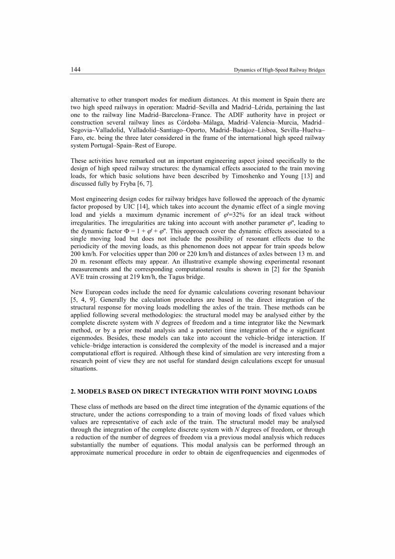
vibration. This kind of procedures are available in the majority of finite element codes, and for certain cases of simple structures the spectral analysis can be achieved by analytical methods. Finite element methods are applicable to arbitrary structures, even when non linear effects must be considered. A spatial semidiscretisation of the structure is performed into subdomains called “finite elements” leading a discrete N-d.o.f. system of equations: ( )tfddd =++ KCM &&& (1) where M is the mass matrix, C is the damping matrix, K is the stiffness matrix, f(t) is the vector of external loads, and d is the unknown vector of nodal displacements. In order to integrate in time this system of equations, a direct integration of the model solves the complete system (1) for each time step, and because the equations are generally coupled they must be solved simultaneously. This procedure is valid even when nonlinear effects must be taken into account. In such case the elastic internal forces and viscous damping should be replaced by a general nonlinear term ( )ddf &,int . If as usual the structural behaviour is linear, a modal analysis can be performed resulting in another system with a remarkable reduction of degrees of freedom. In a first stage, the eigenvalue problem corresponding to the undamped system is performed solving the generalised eigenproblem corresponding to the structural discrete system: ( ) 0KM2 =+− aω (2) obtaining the more significant n eigenfrequencies nii 1...=ω , and the corresponding normal vibration modes an, being generally n << N. In a second stage, the vibration modes ai oscillating with their respective frequencies ωi are integrated in time. With this procedure the equations are decouple, and the modal response of each mode is obtained from the dynamic equation of a system with a single degree of freedom. The simplest procedure to define the train loads is applying load histories in each node. For time step ti and an axle load F, a nodal load FJ is assigned to the node J if the axle is above an element that contains node J. The magnitude of FJ depends linearly on the distance from the axle to the node. This procedure is outlined in Figure 1 for a single load. This scheme has been implemented in the finite element program FEAP [12] both for the ten HSLM–A (High Speed Load Model) trains defined in the Eurocode [4, 9] and for the seven real trains defined in the Spanish code IAPF [9]. All the results for point moving loads described in this paper have been obtained with the methodology described in this section, using a direct time integration of the significant eigenmodes.


Figure 1: Nodal force time history definition for an axle load F moving at velocity v

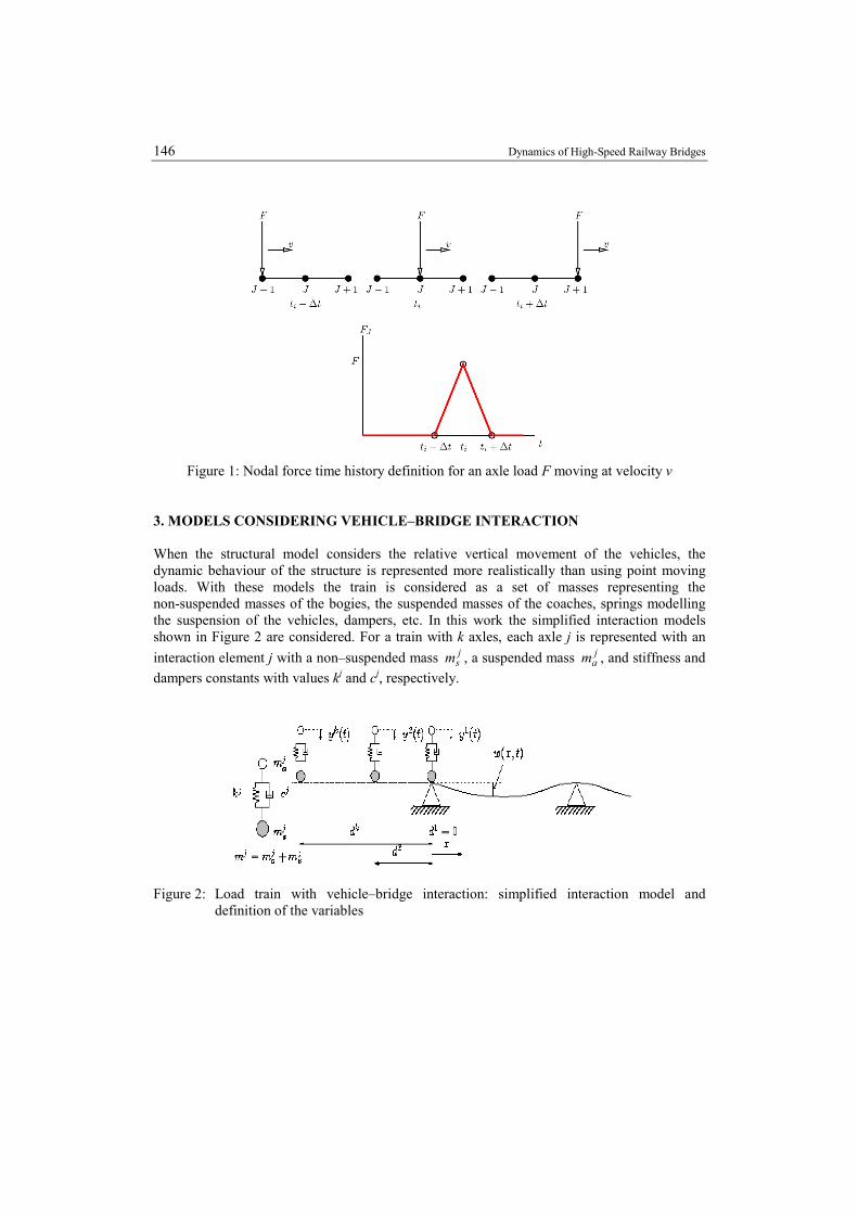
3. MODELS CONSIDERING VEHICLE–BRIDGE INTERACTION When the structural model considers the relative vertical movement of the vehicles, the dynamic behaviour of the structure is represented more realistically than using point moving loads. With these models the train is considered as a set of masses representing the non-suspended masses of the bogies, the suspended masses of the coaches, springs modelling the suspension of the vehicles, dampers, etc. In this work the simplified interaction models shown in Figure 2 are considered. For a train with k axles, each axle j is represented with an interaction element j with a non–suspended mass j

sm , a suspended mass jam , and stiffness and

dampers constants with values kj and cj, respectively.

Figure 2: Load train with vehicle–bridge interaction: simplified interaction model and

definition of the variables


The equations obtained for the structure and the vehicle are (3) and (4), respectively:

⎭⎬⎫

⎩⎨⎧

+

=⎪⎭

⎪⎬⎫

⎪⎩

⎪⎨⎧

⎟⎟

⎠

⎞

⎜⎜

⎝

⎛+

⎪⎭

⎪⎬⎫

⎪⎩

⎪⎨⎧

⎟⎟

⎠

⎞

⎜⎜

⎝

⎛+

⎪⎭

⎪⎬⎫

⎪⎩

⎪⎨⎧

⎟⎟

⎠

⎞

⎜⎜

⎝

⎛

extw,B

arw,B

wBBBW

WBWW

wBBBW

WBWW

wBBBW

WBWW

W

ff

b

w

b

w

b

w

f

KK

KK

CC

CC

MM

MM

&

&

&&

&&

(3)

⎭⎬⎫

⎩⎨⎧ +

=⎪⎭

⎪⎬⎫

⎪⎩

⎪⎨⎧

⎟⎟

⎠

⎞

⎜⎜

⎝

⎛+

⎪⎭

⎪⎬⎫

⎪⎩

⎪⎨⎧

⎟⎟

⎠

⎞

⎜⎜

⎝

⎛+

⎪⎭

⎪⎬⎫

⎪⎩

⎪⎨⎧

⎟⎟

⎠

⎞

⎜⎜

⎝

⎛

exty,B

ary,B

YYYB

BYyBB

YYYB

BYyBB

YYYB

BYyBB

Y

ff

y

b

y

b

y

b

f

KK

KK

CC

CC

MM

MM

&

&

&&

&&

(4)

In these equations the degrees of freedom have been got into three groups corresponding to the nodes modelling the contact of the train with the deck (b), the rest of the nodes of the deck (w), and those corresponding to the suspended masses of the vehicle (y). In the load vector modelling the wheel–deck forces, the contribution of the action–reaction term (f .,ar) and the external loads have been distinguished (f .,ext). 3.1 Time integration based on the modal decomposition The solution of the equation (3) can be expressed:

( )( ) ( )( )( )( )( )⎪⎭

⎪⎬⎫

⎪⎩

⎪⎨⎧

=⎪⎭

⎪⎬⎫

⎪⎩

⎪⎨⎧

∑= tx

txtqttx

kB

kWN

iik

i

i

φ

φ

1,

b

w (5)

being qi = qi(t) the modal amplitude, N the number of modes used in the analysis,

iWφ and iBφ

the components of the eigenvector i corresponding to the degrees of freedom w and b respectively, and xk(t) the parameter of position of the axle k. Normalising the eigenvectors with the mass matrix, the modal equations are:

Niqqq,,

T

iiiiiii

i ..., 12extW

BarW

B

W

B

W2 =⎪⎭

⎪⎬⎫

⎪⎩

⎪⎨⎧

+⎪⎭

⎪⎬⎫

⎪⎩

⎪⎨⎧

=++ff

f

φ

φωωξ &&& (6)

Solving for ary,

Bf in (4) and substituting ary,B

arWB ff −=, , results:

bybybyff y

BBBYyBBBY

yBBBY

exty,B

arwB KKCCMM −−−−−−= &&&&&&, (7)


The equation (6) is re-written via the substitution of the modal expression of b detailed in (5), in equation (7):

{ }

{ }

{ }∑

∑

∑

=

=

=

−

′+−

′′+′+−

−−−+=++

N

jj

N

jjj

N

jjjj

iiii

ji

jji

jjji

iiiii

q

vqq

qvqvq

Kffqqxq

1B

yBBB

1BB

yBBB

1B

2BB

yBBB

BYBBYBBYBext

BBWW2

2

2

φφ

φφφ

φφφφ

φφφφφωω

K

C

M

CM

&

&&&

&&&&&& yyy

(8)

being: tvxy k =+= exty,

Bextx,

Bext

B fff (with the hypothesis of constant velocity of the train). In order to integrate the movement of the suspended masses the modal expression of b is substituted in (4), resulting the system of differential equations:

{ }

{ }

{ }∑

∑

∑

=

=

=

−

′+−

′′+′+−=++

N

jj

N

jjj

N

jjj

j

jj

jjj

q

vqq

qvqvq

1BYB

1BBYB

1B

2BBYBYYYYYYY 2

φ

φφ

φφφ

K

C

´MfKCM

&

&&&&&& yyy

(9)

The equations (8) and (9) must be integrated in order to obtain the modal amplitudes qj(t) and the degrees of freedom of the suspended masses y(t). After this, the degrees of freedom corresponding to the movement of the deck (w and b) are computed from equation (5). 3.2 Direct time integration In order to carry out the time integration of the whole structure, taking into account all its degrees of freedom, a model based on the Euler–Bernoulli beam with an additional degree of freedom corresponding to the axle of the train was developed (see Figure 3). Let w1, θ1, w2, θ2 denote the degrees of freedom of the beam (displacement and rotation of the nodes), and y and b the degrees of freedom of the suspended mass (mv) and the non–suspended one (mw) respectively. The dynamical equilibrium equations of the element are:

⎪⎭

⎪⎬⎫

⎪⎩

⎪⎨⎧

=⎪⎭

⎪⎬⎫

⎪⎩

⎪⎨⎧

+⎪⎭

⎪⎬⎫

⎪⎩

⎪⎨⎧

+⎪⎭

⎪⎬⎫

⎪⎩

⎪⎨⎧

b

y

F

F

b

y

b

y

b

yinteracinteracinterac KCM

&

&

&&

&& (10)


being:

⎟⎟

⎠

⎞

⎜⎜

⎝

⎛

−

−=

⎟⎟

⎠

⎞

⎜⎜

⎝

⎛

−

−=

⎟⎟

⎠

⎞

⎜⎜

⎝

⎛=

vv

vv

vv

vv

w

v

kk

kk

cc

cc

m

minteracinteracinterac

0

0K,C,M (11)

Figure 3: Bernoulli beam element with simplified vehicle–bridge interaction model

The displacement of the non–suspended mass b is interpolated from the nodal displacements of the beam in a standard way via the hermitic shape functions [15]:

[ ]

⎪⎪⎪

⎭

⎪⎪⎪

⎬

⎫

⎪⎪⎪

⎩

⎪⎪⎪

⎨

⎧

=

2

2

1

1

4321

θ

θ

w

w

NNNNb (12)

Using the transformation matrix T:

⎟⎟

⎠

⎞

⎜⎜

⎝

⎛=

4321 0

00100

NNNNT (13)

The motion equations of the element result [8]:

⎪⎪⎪⎪

⎭

⎪⎪⎪⎪

⎬

⎫

⎪⎪⎪⎪

⎩

⎪⎪⎪⎪

⎨

⎧

+

⎪⎪⎪⎪

⎭

⎪⎪⎪⎪

⎬

⎫

⎪⎪⎪⎪

⎩

⎪⎪⎪⎪

⎨

⎧

+

⎪⎪⎪⎪

⎭

⎪⎪⎪⎪

⎬

⎫

⎪⎪⎪⎪

⎩

⎪⎪⎪⎪

⎨

⎧

=

⎪⎪⎪⎪

⎭

⎪⎪⎪⎪

⎬

⎫

⎪⎪⎪⎪

⎩

⎪⎪⎪⎪

⎨

⎧

2

2

1

1

2

2

1

1

2

2

1

1

2

2

1

1

θ

θ

θ

θ

θ

θ

w

y

w

w

y

w

w

y

w

M

F

F

M

F

y KCM

&

&

&

&

&

&&

&&

&&

&&

&&

(14)

being: TKTKT,CTCT,MTM interacinteracinterac

TTT === (15)


The matrix (15) must be assembled with the standard matrix of the Bernoulli beam element in order to obtain the stiffness matrix of the interaction element. The element matrix must be re-computed in each time step. 4. APPLICATION: DYNAMIC ANALYSES OF SHORT SPAN BRIDGES In these analyses four short span bridges defined in the ERRI 214 catalogue of isostatic bridges have been considered. The definition of the bridges is summarised in Table 1. The loads considered was the corresponding to the ICE 350 E high speed train, that will run in Spain with the name AVE 103, in the range of velocities from 120 km/h. to 420 km/h. The same damping ratio ξ = 2% has been adopted for all the calculations.

Table 1: Definition of short span bridges from ERRI D214 catalogue. Length (m) Mass (kg ×103/m) Frequency (Hz) EI (kNm2)

5.0 7 16 453919 7.5 9 12 1661921

10.0 10 8 2593823 20.0 20 4 50660592

The curves in Figures 4 and 5 correspond to the envelopes of accelerations and displacements in the mid point of the 7.5 m. span. It can be observed a left translation of the peaks computed with the interaction model relative to the point load results. This effect appears because the interaction models include the mass of the vehicle leading to the reduction of the frequencies of the viaduct (if both masses have similar values). Besides, a reduction in the highest values of accelerations and displacement is obtained when using interaction models.

Figure 4: Acceleration and displacement in the mid span of the 7.5 m. beam

With the standard finite element formulation of the Euler–Bernoulli beam element [15] the expression of the terms in the mass matrix is:


∫∫ +=L jiL xjxiij dxNNAdxNNIM ρρ ,, (16)

The first term in the right hand side of equation (16) corresponds to the rotational part of the mass matrix (Mrot), and the second term contributes to the translational part (Mtras), being M = Mrot + Mtras. The contribution of Mrot to M is very small for long span bridges. Nevertheless, although this term is neglected by several computational codes, it is important in short span bridges. This fact is shown in Table 2 where the values of the first frequency of an isostatic beam are reported for several lengths.

Figure 5: Acceleration and displacement in the mid span of the 7.5 m. beam

Table 2: First frequency of an isostatic beam considering/not considering the rotational mass

matrix Frequency (Hz)

Length (m) with R.M. without R.M. 5.0 13.5478 16.0000 7.5 11.0682 12.0000

10.0 7.6322 8.0000 20.0 3.9515 4.0000

Figure 6 shows the comparison between the envelopes of displacements for the spans of L = 5.0 m. and L = 20.0 m. It has been considered models with rotational mass and without it, using both point loads as vehicle–bridge interaction elements. For the 5 m. span bridge, comparing the results obtained with rotational mass (black and blue curves) with those obtained without it (red and yellow curves) an important translation to the left side is observed for the models with rotational mass. The reason is the remarkable increment of the structural mass associated to the rotational terms. Comparing, for the same formulation of the mass matrix, the results obtained using point moving loads with those obtained with interaction models (the black curve versus the blue one, and the red curve versus


the yellow one) another translation of the resonant peaks is observed, although less relevant than in the former comparison. Finally, for the 20 m. span can be concluded that the contribution of the rotational is negligible from a practical point of view.

Figure 6: Vertical displacement in the midspan: L = 5 and L = 20 m.

5. DYNAMIC ANALYSIS OF AN ARCH BRIDGE 5.1 Description of the structure and modelling In this section the results obtained from the dynamic analysis of an arch bridge, in design stage for the Ourense–Santiago high speed line, are shown. This viaduct is formed by a concrete arch


with a span of 170 m. and a deck with length 630 m. The deck and the arch are connected with five piles. The material used for the arch and deck is concrete H40 (characteristic resistance fck = 40 kN/mm2) and for the piles concrete H30 (fck = 30 kN/mm2). The area and moment of inertia of the arch are 7.76 m2 and 14.87 m4, respectively. For the deck these values are A = 11.25 m2 and I = 25.91 m4. The dynamic analysis was carried out with a 2D finite element model. The model have 1639 beam elements, leading to a system with 4872 degrees of freedom. All the computations have been carried out with the finite element code iris [11]. The mesh of the model is showed in Figure 7. The joins of the piles with the deck are encastred, having the pile in this point the same rotation that the deck. In the left end support the horizontal displacement and bending rotation are allowed, and the right end support is a fixed point.

Figure 7: Arch bridge. Finite element model

For the time integration the first 114 eigenmodes have been considered in order to take into account all the frequencies lower than 30 Hz., and a modal damping ξ = 2% has been assigned to all the modes. Figure 8 shows the four lower eigenmodes computed.

f1 = 0.954 Hz f2 = 1.396 Hz

f3 = 1.477 Hz f4 = 1.577 Hz

Figure 8: Arch bridge. First to fourth eigenmodes


5.2 Results The calculations ere performed for a range of velocities of 120-420 km/h every ∆v=5 km/h, considering the following high speed trains:

1. The ten trains corresponding to the HSLM-A (High Speed Load Model) IAPF 2003 [9] and Eurocode [4].

2. The seven European high speed trains defined in the Spanish IAPF code [9]: AVE, EUROSTAR 373/1, ETR-Y, ICE-2, TALGO-AV, THALYS and VIRGIN, modelled with moving point loads.

3. The AVE 103 Spanish high speed train modelled both with moving point loads as with simplified interaction elements, in order to compare the results obtained with these methodologies.

Figures 9 and 10 show the displacements and acceleration in the centre of the 3rd span obtained with the AVE-103 train (with and without interaction). Figures 9 and 10 show these variables in the keystone of the arch.

Figure 9: Arch bridge. Displacements in the 3rd midspan

Figure 10: Arch bridge. Accelerations in the 3rd midspan


Figure 11: Arch bridge. Displacements in the keystone of the arch

Figure 12: Arch bridge. Accelerations in the keystone of the arch

It can be observed from these figures that the dynamical effects are more relevant in the keystone of the arch. Besides there isn’t reduction of the dynamical effects with the interaction models because the spans of the structure have moderately long lengths. Figures 13 and 14 show the bending moments in the left support and in the keystone of the arch respectively, computed both for the seven real trains defined in the Spanish code IAPF [9] and for the ten HSLM-A (High Speed Load Model) trains defined in the Eurocode [4, 9]. By a direct comparison of the highest dynamical values with the static envelopes in each point the dynamic amplification factor obtained is ≈2.5.


Figure 13: Arch bridge. Bending moments in the left support of the arch

5.3. Conclusions The two principals eigenmodes mainly contain the deformation of the arch. Their frequencies are lower than those usual in standard bridges with shorter lengths. The first mode (f1 = 0.954 Hz) leads to non symmetric movements and the second mode (f2 = 1.396 Hz) is symmetric. The following modes correspond to the movement of the deck and the piles, and in consequence is convenient to take into account the dynamical effects in these elements. Resonant effects could appear for low velocities due to the low values of the main frequencies. Nevertheless, because the wave length of the first modes (≈170 m.) is one order of magnitude higher than the length of the train coaches (between 13 and 27 m.) there are simultaneously several axle loads in the bridge and therefore their effects are mutually cancelled. Finally, in this structure the consideration of interaction model is not relevant because the results obtained are very similar with those computed with point moving loads.


Figure 14: Arch bridge. Bending moments in the keystone of the arch

6. DYNAMIC ANALYSIS OF A PERGOLA BRIDGE 6.1 Description of the structure and modelling This viaduct will be in the Madrid–Valencia high speed line. It is a pergola bridge composed of 64 attached longitudinal beams with box section typology. The length of the precasted beams varies from 35.35 m. of the shortest one to 40.62 m. The separation between the axles of the beams is 4.5 or 6 m., leading to 326.75 m. of total width. In order to verify the requirements in the Spanish IAPF code [9] and Eurocode 1 [4], the dynamic analysis comprises the following points:

1. Determination of the impact coefficient for velocities lower than 220 km/h, via simplified methods.

2. Determination of the impact coefficient for velocities higher than 220 km/h, via dynamic calculations. These computations consider the following aspects:


• Time integration of all the eigenmodes with frequencies lower than 30 Hz. • The actions applied are the corresponding to the ten trains of the HSLM-A

model (High Speed Load Model A) defined in [4, 9], which are dynamic envelopes of the effects of the possible real trains.

• The calculations are performed for a range of velocities of 120-300 km/h every ∆v=5 km/h. The highest velocity is 20% higher than the design velocity vdesign = 250 km/h.

3. Verification of the ELS (Usage Limit State) requirements for the maximum values of acceleration, vertical displacements and rotations

Taking into account the dimensions and typology of the viaduct, and because the tracks are mainly in transversal direction (see Figure 15), it has been considered convenient to perform a three dimensional finite element model.

Figure 15: Pergola bridge. General plant view

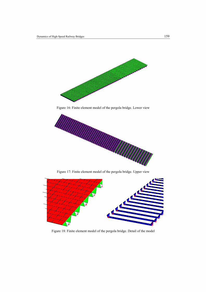
This bridge has been modelled with 7220 four nodes shell elements and 6342 nodes leading to a model with 37730 degrees of freedom. Figures 16 and 17 show a general view of the mesh. The boundary conditions adopted correspond to a point support of the ends of each beam as is showed in the detail of Figure 18. For the evaluation of the vibrating mass of the viaduct it has been considered the mass of concrete and the added masses corresponding to other non-structural members (ballast, sleepers, rails, etc). The values adopted for the mechanical properties of concrete are Young modulus E = 3.5 GPa and Poison ratio ν = 0.2.


Figure 16: Finite element model of the pergola bridge. Lower view

Figure 17: Finite element model of the pergola bridge. Upper view

Figure 18: Finite element model of the pergola bridge. Detail of the model


6.2 Dynamic analysis of the structure The dynamic analysis of the structure has been performed in accord to the requirements in the appendix B of IAPF 2003 code [9], via the time integration of the modes of oscillation of the structure. In order to take into account all the modes with associated eigenfrequencies lower than 30 Hz, it is necessary to consider 552 eigenmodes in the dynamic computations. The deformed shapes corresponding to the fourth lower modes of oscillation are showed in figure 19. The damping is defined as Rayleigh damping [1] considering a fraction of critical damping rate ξ equal to 2% (for concrete structures). The applied loads correspond to the 10 trains defined in the HSLM-A model for a range of velocities from 120 km/h to 300 km/h every 5 km/h, leading to 370 analyses with 552 eigenmodes each one. To perform this computations in a reasonable lapse of time they have been used 24 PENTIUM machines, with 2.6 GHz and 512 Mb RAM, running in parallel processes. The results obtained from each one of the 370 analyses have been post-processed in order to obtain the maximum values of vertical displacement, vertical acceleration and “in plane” rotations. These maximum values have been considered for reporting the results obtained in the following sections. 6.3 Simplified calculation of the impact coefficient The simplified methodology for the evaluation of the impact coefficient Φ2 described in the IAPF 2003 code [9] is only valid for velocities lower than 220 km/h, and has the following requirements:

1. The typology of the viaduct must be conventional. 2. The first eigenfrequency must be valued between the two bounds defined in the

expression (2.5) of the IAPF 2003 code [9]. For the particular case of this viaduct the lower bound is fmin = 2.73 Hz and the upper one fmax = 6.23 Hz. Therefore the first frequency of the viaduct (f1 = 4.31 Hz) verifies this requirement. For structures with good maintenance the expression of the simplified impact coefficient is:

06182020

4412 ..

..

=+−

=ΦΦL

(17)

being LΦ defined in the IAPF 2003 [9] as the "characteristic length” of the viaduct (for this bridge LΦ = 38 m). 6.4 Calculation of the impact coefficient from dynamic analysis The Spanish IAPF 2003 code requires a complete and specific dynamic analysis of structures in high speed lines with design velocity upper than 220 km/h. From the results of this analysis


using the high speed trains, an impact coefficient Φ must be obtained. This impact coefficient Φ will be compared with the impact coefficient Φ2 from expression (17), and the coefficient with the highest value will be considered for the design of the structure. From the dynamic analysis results, the real impact coefficient of the train i in some point of the structures is:

( )tipoest,

reldin,501δδ

ϕi

i ′′+=Φ . (18)

being i

reldin,δ the maximum movement obtained for the train i, tipoest,δ the movement obtained statically using the train defined in the IAPF 2003 (“tren tipo”) from the UIC train, and ϕ'' a coefficient related to the tracking irregularities [3] (in this bridge ϕ''=0.0141). Figure 20 shows the impact coefficient Φ obtained applying the expression (18) for each velocity and each train. The impact coefficient is the highest value obtained considering all the trains, and in this structure is the one obtained with the HSLM-A9 train running with a velocity v = 290 km/h: 5170max .=Φ=Φ i

i (19)

Comparing this value of Φ with the one obtained in (17) using the simplified methodology results the impact coefficient to consider in the design of the viaduct: 061.=Φ (20) 6.5 Verification of the usage limit state The deformations, displacements and accelerations in the deck of railway bridges are related to the Usage Limit States for the structure, and to the Ultimate Limit State of the track and vehicles [10]. For this reason in the IAPF 2003 and Eurocode [9, 4] are included the Usage Limit States that must be considered in order to avoid security problems. Accelerations In accord to the section 4.2.1.1.1 of IAPF 2003 and section A.2.4.4.2.1 of Eurocode 1, the maximum vertical acceleration of the deck must verify: ga 350max .≤ (21) for bridges with ballast. In accord to [3], the values obtained from the dynamic computations (for an ideal track) must be incremented by a factor (1+0.5ϕ'') in order to take into account the


track irregularities. The maximum values of the acceleration are showed in Table 3. From these results can be concluded that the structure verifies the requirement (21).

Table 3: Pergola bridge. Maximum values of the vertical acceleration Train a (m/s2) a (m/s2)

HSLM A01 1.89 (v=250 km/h) 2.01 (v=260 km/h) HSLM A02 2.41 (v=265 km/h) 3.00 (v=285 km/h) HSLM A03 1.89 (v=290 km/h) 2.19 (v=300 km/h) HSLM A04 2.97 (v=295 km/h) 2.98 (v=300 km/h) HSLM A05 1.92 (v=290 km/h) 1.79 (v=295 km/h) HSLM A06 1.95 (v=285 km/h) 1.79 (v=290 km/h) HSLM A07 2.16 (v=290 km/h) 1.87 (v=295 km/h) HSLM A08 1.52 (v=265 km/h) 2.57 (v=295 km/h) HSLM A09 1.95 (v=290 km/h) 1.98 (v=295 km/h) HSLM A10 2.06 (v=285 km/h) 2.22 (v=295 km/h)

Rotations of the deck For bridges with double track and ballast the values of the rotation in the transition tie bar–deck are bounded with the value [9, 4]: rad1053 3−⋅≤ .θ (22) Figure 21 shows the envelopes of the rotations both in the incoming as the out-coming tie bars of the bridge. It can be verified that the computed values are two orders of magnitude lower than the required one. Comfort In section 4.2.1.2 of the IAPF 2003 code [9] the values of the vertical displacements are limited in order to ensure the comfort of the passengers. Besides the comfort level is classified in accord to the maximum values obtained for the vertical acceleration. In this bridge the maximum acceleration has a value upper than 2.0 m/s2, and therefore the comfort level is considered as “allowable”. The requirements for comfort are established in terms of the ratio L/δ, being L the length and δ the maximum vertical displacement. The value of this ratio must be corrected with a factor that depends on the maximum acceleration value and the number of spans. For the Pergola bridge described in this paper the comfort requirements are satisfied.


f1 = 4.31 Hz f2 = 4.43 Hz

f3 = 4.51 Hz f4 = 4.52 Hz

f5 = 4.57 Hz f6 = 4.63 Hz

Figure 19: Pergola bridge. First to fourth eigenmodes


Figure 20: Pergola bridge. Impact coefficient Φ in the midpoint of the track

Figure 21: Pergola bridge. Envelopes of rotation in the tie bar–deck transition


ACKNOWLEDGEMENTS The authors acknowledge the financial support of Ministerio de Fomento of Spain to the project “Análisis dinámico de estructuras sometidas a acciones de trenes de alta velocidad” through the research program “Acciones Estratégicas del Área Sectorial de Construcción Civil y Conservación del Patrimonio Histórico Cultural” of the “Plan Nacional de Investigación Científica, Desarrollo e Innovación Tecnológica 2002-2003” 7. REFERENCES

[1] Clough, R.W. and Penzien, J. Dynamics of Structures. Second Edition, McGraw- Hill, 1994.

[2] Domínguez Barbero, J. Dinámica de puentes de ferrocarril para alta velocidad: métodos de cálculo y estudio de la resonancia. Ph. D. thesis (in Spanish). E.T.S. Ingenieros de Caminos, Universidad Politécnica de Madrid. 2001.

[3] ERRI D214 committee. Ponts-rails pour vitesses >200 km/h; Etude Numérique de l’influence des irrégularités de voie dans les cas de résonance des ponts. Rapport technique RP 5. European Rail Research Institute (ERRI). March, 1999.

[4] Eurocode 1. Actions on structures - Part 2: Traffic loads on bridges. CEN, 2003. [5] Ferrovie dello Stato, Italy. Sovraccarichi per il calcolo dei ponti ferroviari.

Istruzioni per la progettazione, l’esecuzione e il collaudo. Code I/SC/PS-OM/2298. 1997.

[6] Fryba, L. Vibration of solids and structures under moving loads. Academia, Noordhoff. 1972.

[7] Fryba, L. Dynamics of railway bridges. Thomas Telford. 1996. [8] Ju, S. and Lin, H. Numerical Investigation of a steel arch bridge and interaction

with high-speed trains. Engineering Structures. Vol 25. pp. 241-250, (2003). [9] Ministerio de Fomento, Spain. Instrucción de acciones a considerar en el proyecto

de puentes de ferrocarril. Draft J.. 2003. [10] Nasarre y de Goicochea, J. Estados límites de servicio en relación con la vía en

puentes de ferrocarril. Puentes de Ferrocarril. Proyecto, Construcción y Mantenimiento. Congreso del Grupo Español de IABSE. Vol 2. Madrid, Junio de 2002.

[11] Romero, I. iris: User Manual. Universidad Politécnica de Madrid. http://w3.mecanica.upm.es/~ignacio/iris.html.

[12] Taylor, R.L. FEAP. A Finite Element Analysis Program. University of California, Berkeley. http://www.ce.berkeley.edu/~rlt/feap.

[13] Timoshenko, S. and Young, D. Vibration problems in engineering. Van Nostrand, 3rd ed. 1995.

[14] Union Internationale des Chemins de Fer. Charges a prendre en considerations dans le calcul des ponts-rail. Code UIC 776-1R. 1979.

[15] O.C. Zienkiewicz and R.L. Taylor, The finite element method, Butterworth-Heinemann, (2000).

dynamic analysis of structures under high speed …

Documents