Dynamic Asset Allocation Strategies Using

a Stochastic Dynamic Programming Approach∗

Gerd Infanger†

Department of Management Science and EngineeringStanford University

Stanford, CA 94305-4026and

Infanger Investment Technology, LLC2680 Bayshore Parkway, Suite 206

Mountain View, CA 94043

AbstractA major investment decision for individual and institutional investors alike is to

choose between different asset classes, i.e., equity investments and interest-bearing in-vestments. The asset allocation decision determines the ultimate risk and return of aportfolio. The asset allocation problem is frequently addressed either through a staticanalysis, based on Markowitz’ mean-variance model, or dynamically but often myopi-cally through the application of analytical results for special classes of utility functions,e.g., Samuelson’s fixed-mix result for constant relative risk aversion. Only recently, thefull dynamic and multi-dimensional nature of the asset allocation problem could becaptured through applications of stochastic dynamic programming and stochastic pro-gramming techniques, the latter being discussed in various chapters of this book. Thepaper reviews the different approaches to asset allocation and presents a novel approachbased on stochastic dynamic programming and Monte Carlo sampling that permits oneto consider many rebalancing periods, many asset classes, dynamic cash flows, and ageneral representation of investor risk preference. The paper further presents a novel ap-proach of representing utility by directly modeling risk aversion as a function of wealth,and thus provides a general framework for representing investor preference. The papershows how the optimal asset allocation depends on the investment horizon, wealth, andthe investor’s risk preference and how it therefore changes over time depending on cashflow and the returns achieved. The paper demonstrates how dynamic asset allocationleads to superior results compared to static or myopic techniques. Examples of dynamicstrategies for various typical risk preferences and multiple asset classes are presented.

Keywords: portfolio theory and applications, dynamic asset allocation, stochastic dynamic pro-gramming, stochastic programming.JEL Classifications: C61, D81, G1.

∗ to appear in Handbook of Asset and Liability Management, S. Zenios and W.T. Ziemba (Eds.), Elsevier,Amsterdam, 2006.

† Dr. Gerd Infanger is a Consulting Professor of Management Science and Engineering at StanfordUniversity and Founder and CEO of Infanger Investment Technology, LLC.

1

1 Introduction

The major decision of an investor regarding his/her portfolio is to choose the allocationbetween different asset classes, especially between equity investments and interest-bearinginvestments. Strategic asset allocation determines the ultimate expected rate of return andrisk of an investor’s portfolio, see, e.g., Blake et al. (1999). For individuals and institutionalinvestors alike, it is usually a long-term decision and its analysis should include all financialaspects, e.g., wealth, current and future cash flows, and financial goals. Inflation, as well asliquidity considerations (to plan for the unexpected), should be part of the analysis.

In the long run, equity investments have grown at a faster rate than other assets suchas bonds, T-bills, and inflation, see, e.g., Siegel (2002), Constantinides (2002), and Dimson,Marsh and Staunton (2002). However, in the short run, the risk is significant and may leadto negative returns. Even in the long run, equity investments can be quite risky, and aswe have painfully observed during the recent downturn from 2000 till 2003 as well as inbear markets before, equity investments can quickly lose a significant portion of their value.interest-bearing investments have exhibited lower returns in the long run, barely exceedinginflation, but with less risk, making them possibly a better vehicle for the short-term. Itis clear that one needs to determine the right balance between the asset classes, and thisbalance depends on how much risk an investor is willing to assume and may change overtime due to changes in wealth, needs, goals and market conditions. It is well known thatstrategic asset allocation has a far greater impact on the overall performance of an investor’sportfolio than, for example, the selection of individual securities.

The question of how the length of the investment horizon impacts the optimal assetallocation is an important theoretical and practical question, which has been discussed in theacademic literature for more than 30 years. The answers to this question vary significantlydepending on the assumptions made. For example, Levy (1972) and Gunthorpe and Levy(1994) discussed portfolio performance and composition versus investment horizon in amean-variance framework. Practitioners tend to recommend a larger allocation towardsstocks as the investment horizon increases. This is often argued under the name of “timediversification”, and is based on the argument that if stocks are distributed independentlyand identically in each time period according to a log normal distribution, the distributionover many periods as the product of log normals is also log normal and the mean and thevariance of the logarithm of the return distribution grows proportionally with the lengthof the investment period. Since the standard deviation of the log returns then grows withthe square root of the horizon, the probability of capital loss decreases as time increases,and stocks become more favorable as the time horizon increases. Using this argument witha reasonable assumption of a 10% mean and 15% volatility, annually, one may verify thatafter an investment horizon of about seven years, the return on stocks exceeded with 95%probability is positive. It would takes 13 years to arrive at a positive return exceeded with99% probability.

Time diversification often includes a broader view of human capital, suggesting thatthe capital represented by an individual’s ability to work and generate wages should alsoenter the equation. Consequently, at the beginning of one’s professional life, most of one’scapital is the potential of generating future income through labor, which is consideredto be not risky, while at the end of one’s professional career, most capital lies in one’s

2

financial assets (in the retirement account, but also real estate, stocks, etc.), and the abilityto work and to generate income becomes a lesser part of the total capital. Thus, it isargued that at the beginning of one’s career, the small amount in financial assets shouldbe invested in a more risky allocation and gradually reduced to a less risky allocation atretirement, when all assets are the financial assets generated during the lifetime. Based ontime diversification arguments, a common rule of thumb used by practitioners is to investin stocks the percentage resulting from 100 - age, thus a 30 year old should invest about70% of his portfolio into stocks, and a 60 year old about 40%. These arguments only usetime as the explaining factor and the corresponding strategies do not react to investmentperformance.

Treynor (2003) on time diversification puts forward the question of how each year’sinvestment choices influence the wealth accumulated at the end of one’s career. This per-spective concludes that the impact of each year’s dollar gains and losses on terminal wealthdepend on the riskless rate, and one should time diversify in such a way that the risk evalu-ated in terminal dollars should be constant over the investment horizon. Therefore, unlessinvestors can predict different returns for each year, the money amount exposed to the stockmarket should be approximately constant over the life-time.

Samuelson (1969) in his landmark work addressed how much of his/her wealth an indi-vidual should either consume or invest at any period in time, assuming no bequest is to beleft behind. He proves using a backward dynamic programming recursion that, given thechoice of one risky asset and one risk free asset, for the returns of the risky asset distributedidentically and independently (iid) over time, for all income generated through investment,and for individuals valuing their consumption in time according to a power utility functionwith respect to consumption and maximizing discounted expected utility over the lifetime,it is optimal to invest the same proportion of wealth into stocks in every period, indepen-dently of wealth. The same was proved by Merton (1969) in continuous time and later,see Merton (1990), extended to multiple risky assets and various bequest situations. Thislife-time portfolio and consumption selection prompted an apparent conflict between theo-reticians and practitioners, since the advice from Samuelson and Merton is quite differentfrom what financial practitioners tell their clients. The remarkable aspect of Samuelson’sand Merton’s result is that, under their assumptions about the market and under constantrelative risk aversion, the consumption decisions and the investment decisions are indepen-dent of each other, and therefore the optimal investment decision is not only invariant withrespect to investment horizon but also with respect to wealth. Thus, the result translatesdirectly to the investment problem only, where one wants to maximize the utility of finalwealth at the end of the investment horizon, by allocating and re-allocating at each periodalong the way. The result follows directly from the utility function used, stipulating thatthe (relative) risk aversion of the individual is invariant with respect to wealth.

Optimal multi-period investment strategies based on maximizing expected utility havebeen analyzed by Mossin (1968). Mossin’s research attempted to isolate the class of utilityfunctions of terminal wealth which result in myopic utility (value) functions for intermediatewealth positions. For a discussion of utility functions, see Section 4 below. Myopic meansthat these functions are independent of returns beyond the current period. Thus, it wouldbe sufficient to analyze only the current optimization problem to arrive at an optimalmulti-period investment strategy. Mossin concluded that logarithmic functions (for general

3

asset distributions) and power functions (for serially independent asset distributions) arecompletely myopic. He also contended that, if there is a riskless asset (whose return isknown for the entire investment horizon), and a risky one, all utility functions for whichthe risk tolerance is linear in wealth (HARA) would lead to partial myopia as one wouldoptimally invest in any period as if in all further periods the investment were to be madein the riskless asset, and complete myopia would exist if the risk-free rate were to be zero.However, Hakansson (1971) demonstrated that, for the HARA case, even when asset returnsare serially independent, no myopic strategies are optimal, except for the highly restrictedcase of a complete absence of any restrictions on short sales and borrowing. A percentagemargin requirement, an absolute limit on borrowing, or a reasonable lending constraint suchthat the borrowed money would have to be repaid would not lead to a myopic strategy. Thus,in the presence of such restrictions only the power and logarithmic utility functions wouldlead to myopia. Furthermore, if asset returns are serially correlated, only the logarithmicutility function would result in a myopic policy. Later, Cox and Huang (1989) presentedan analytical solution based on diffusion processes for the consumption-investment problemwith HARA utility function and wealth and consumption constrained to be nonnegative.Later, an approach using approximate analytical solutions has been developed by Campbelland Viciera (2002), based on perturbations of known exact solutions. See also the chapterby Chacko and Neumar (2006) in this book.

Thus we can summarize, a logarithmic utility function results in a myopic portfoliostrategy, both for serially dependent and independent assset return distributions; a powerutility function results in a myopic strategy only in the case of serially independent assetreturns distributions; and a HARA utility function results in a myopic strategy only forserially independent asset return distributions and only in a non-realistic setting of completeabsence of borrowing and short-selling constraints. All other utility functions do not resultin myopic investment strategies for any return distributions.

More recently, numerical dynamic portfolio optimization methods have been developedthat permit one to determine the asset allocation strategy that maximizes an investor’sexpected utility. These new approaches are based on stochastic dynamic programming andstochastic programming and promise to accurately solve for various types of utility functionsand asset return processes.

2 Approaches for Dynamic Asset Allocation

The two major approaches successful in solving practical dynamic asset allocation problemsare stochastic dynamic programming (stochastic control) and stochastic programming. Aswe have discussed above, asset allocation problems under restrictive assumptions can besolved analytically. In practice, fixed-mix strategies are commonly implemented and oftenlead to very good results.

2.1 Multi-Stage Stochastic Programming

The stochastic programming approach can efficiently solve the most general models, wheretransaction costs need to be considered, and the returns distributions have general serialdependency. The stochastic programming approach also lends itself well to the more general

4

asset liability management problem (ALM). Here, liabilities in addition to assets need to beconsidered. This problem is faced by pension funds and insurance companies. Besides assets,pension plans need to consider retirement obligations, which may depend on uncertaineconomic and institutional variables, and insurance companies need to consider uncertainpay-out obligations due to unforseen and often catastrophic events. Asset liability modelsare most useful when both asset returns and liability pay-outs are driven by common, e.g.,economic, factors. In this case ALM represents the only approach that can take into accountdirectly the joint distribution of asset returns and liability cash flows. Lenders operatingin the secondary mortgage market also face a certain kind of ALM problem, when decidingon re-financing their (pools of) mortgages by issuing a portfolio of bonds, callable or non-callable with various maturities. Here the assets are the mortgages bought from banks andthe liabilities are the bonds issued, see e.g., Infanger (1999).

Traditional stochastic programming uses scenario trees to represent possible futureevents. The trees may be constructed by a variety of scenario generation techniques, withthe emphasis on keeping the resulting tree thin but representative of the event distribu-tion in order to arrive at a computationally tractable problem. Often, in later decisionstages of the model, only a very small number of scenarios is used as a representation ofthe distribution leading to very thin sub-trees. Thus, the emphasis is on obtaining a goodfirst-stage solution rather than obtaining an entire accurate policy. Early applications ofstochastic programming for asset allocation are discussed in Mulvey and Vladimirou (1992),formulating financial networks, and Golub et al. (1995). Early applications of stochasticprogramming for dynamic fixed-income strategies are discussed in Zenios (1993), discussingthe management of mortgage-backed securities, Hillier and Eckstein (1993), and Nielsenand Zenios (1996). Early practical applications of stochastic programming for asset lia-bility management are reported in Kusy and Ziemba (1986) for a bank and in Carino etal. (1994) for an insurance company. Ziemba (2003) gives a summary of the stochasticprogramming approach for asset liability management. An approach based on partitioningthe probability space and calculating deterministic bounds was developed by Frauendorfer(1996), and used for bond management and asset liability management. The book edited byWallace and Ziemba (2005) gives publicly available stochastic programming code. Stochas-tic programming software can be best used from within a modeling system, for example,GAMS (Brooke et al. (1988)) provides DECIS (Infanger (1997)) as an integrated stochasticprogramming solver.

Monte Carlo sampling is an efficient way to go when representing multi-dimensionaldistributions. An approach, referred to as decomposition and Monte Carlo sampling, usesMonte Carlo (importance) sampling within a decomposition for estimating Benders cut co-efficients and right-hand sides. This approach has been developed by Dantzig and Glynn(1990) and Infanger (1992). Dantzig and Infanger (1993) show how the approach of decom-position and importance sampling could be used for solving multi-period asset allocationproblems. The success of the sampling within the decomposition approach depends on thetype of serial dependency of the stochastic parameter processes, determining whether ornot cuts can be shared or adjusted between different scenarios of a stage. Infanger (1994)and Infanger and Morton (1996) show that for serial correlation (in form of autoregressiveprocesses) of stochastic parameters, unless in the right hand side of the (linear) program,cut sharing is difficult for more than three decision stage problems. However, for serially

5

independent stochastic parameters, the approach is very efficient for solving problems withmany decision stages.

Monte Carlo pre-sampling uses Monte Carlo sampling to generate a tree, much like thescenario generation methods referred to above, and then employs a suitable method for solv-ing the sampled (and thus approximate) problem. Infanger (1999) used the pre-samplingapproach for representing the mortgage funding problem. This approach combines opti-mization and simulation techniques to represent a 360 month problem by four decisionstages (initial, after a year, after 5 years, and at the end of the horizon) that are subjectto optimization and by pre-defined decision rules representing intermediate decisions. Thepaper also provides an efficient way to independently evaluate the solution strategy as aresult from solving the multi-stage stochastic program to obtain a valid upper bound on theobjective. The pre-sampling approach is general in terms of modeling and solving stochasticprocesses with serial dependency; however, it is limited in the number of decision stages,since problems with many decision stages become computationally difficult. Assuming areasonable sample size for representing the decision tree, problems with up to four decisionstages are meaningfully tractable. Thus, if one were to represent asset allocation problemswith many time (rebalancing) periods, one needed to represent more than one time periodin one decision stage and define rules as to how to manage the assets and liabilities betweendecision stages. For example, one could assume buy and hold between decision stages andallow for rebalancing at the decision stages. In many situations this is considered a suffi-ciently accurate approximation of all future recourse decisions. A stochastic programmingapproach using pre-sampling has been employed by Collomb and Infanger (2005) to ana-lyze the impact of serial dependency on the solution of dynamic asset allocation problems.Instead of pre-defining rebalancing periods up-front, the rebalancing decision may be mod-eled as depending on certain conditions occuring. For example, Mc Lean, Yao and Ziemba(2005) model portfolio rebalancing as conditioned on prices exceeding or going below certainlevels, and Mc Lean, Ziemba and Li (2005) model portfolio rebalancing when certain wealthgoals are met.

In this book, addressing dynamic strategies using stochastic programming for largeinstitutions, Kouwenberg and Zenios (2006) introduce stochastic programming models asthey apply to financial decision making, Mulvey et al. (2006) and Ziemba (2006) discuss theapplication of stochastic programming for multinational insurance companies, Consiglio etal. (2006) discuss the application of stochastic programming for insurance products withguarantees, Edirisinghe (2006) discusses dynamic strategies for money management, andConsigli (2006) discusses the development of stochastic programming models for individualinvestors.

2.2 Stochastic Dynamic Programming

When the focus is on obtaining optimal policies and transaction costs are not the primaryissue, stochastic dynamic programming prooves to be a very effective approach. Stochasticdynamic programming based on Bellman’s (1957) dynamic programming principle has beenused for the derivation of the theoretical results obtained for the HARA class of utilityfunctions discussed above. For general monotone increasing and concave utility functions,no analytical solutions are available. However, stochastic dynamic programming can be

6

used as an efficient numerical algorithm when the state space is small, say, up to threeor four state variables. This limitation in the number of state variables is well known asthe “curse of dimensionality” in dynamic programming. Recently, new methods of valuefunction approximations, see, e.g., De Farias and Van Roy (2003) show promise for problemswith larger state spaces; however, it is unclear at this point in time how accurately thesemethods will approximate the solution of the asset allocation problem. Stochastic dynamicprogramming as a numerical algorithm has been used by Musumeci and Musumeci (1999),representing results with two asset classes, one stock index and a risk free asset, where inthe dynamic programming procedure they condition on the amount of wealth invested inthe risky asset. Earlier, Jeff Adaci (1996) (in a Ph.D. thesis supervised by George Dantzigand the author) conditioned on wealth and thus set the stage for multiple asset classes, butreported results also only for two asset classes and a few periods. Brennam, Schwartz andLagnado (1998) and (1998) proposed a dynamic model using discrete state approximationsincluding four state variables.

In this paper we develop an efficient approach for solving the asset allocation problemunder general utility functions, many time periods (decision stages), and many asset classes.We next review single-period portfolio choice and draw the connections between Markovitz’mean-variance analysis and utility maximization. We then discuss the properties of variousutility functions and present a general framework for modeling utility. Then we discussmulti-period portfolio choice and present a novel approach based on stochastic dynamicprogramming and Monte Carlo sampling.

3 Single-Period Portfolio Choice

Harry Markowitz (1952), in his seminal work, see also Markowitz and van Dijk (2006) inthis book, pointed out that the returns of a portfolio are random parameters and that forthe evaluation of a portfolio, one should consider both its expected returns and its risk,where for representing risk he used the portfolio’s variance. His mean-variance analysis laidthe foundations for modern finance and our understanding as to how markets work. Mean-variance analysis is referred to as modern portfolio theory, whereas post-modern portfoliotheory considers extensions including skewed distributions and asymmetric risk measures.

Let x = (x1, . . . , xn) be the holdings of n asset classes under consideration for a portfolioin a certain time period, and let R = (R1, . . . , Rn) denote the random rates of return of theasset classes, with mean returns r = (r1, . . . , rn), and covariance matrix Σ = [σi,j ], whereσi,j = E(Ri − ri)(Rj − rj) for i, j = 1, . . . , n. Markowitz’s mean-variance model is usuallystated as

min var(RT x) = xT ΣxeT x = 1rTx ≥ ρ

x ≥ 0,

where one chooses the holdings that minimize the variance of the portfolio returns for agiven level of expected return ρ. All portfolios selected by the mean-variance model lieon the mean-variance efficient frontier, i.e., increasing the expected return by moving fromone efficient portfolio to another means risk (measured through variance) also increases, orsmaller risk can only be accomplished by sacrificing expected return.

7

If a risk-free return is present, and for a single-period analysis this is usually assumed tobe the case, then the efficient frontier is represented by the line that intersects the ordinateat the level of the risk-less rate of return and is tangent to the efficient frontier establishedwithout the risk-less asset. The portfolio at the point at which the so called market lineintersects with the original efficient frontier is the market portfolio. The striking result ofTobin’s two fund separation theorem (see Tobin (1958)) is that, if a riskless asset is present,all investors would choose the same portfolio of risky assets, namely the market portfolio,in combination with various amounts of the risk free asset. An investor who wishes toassume the market risk would choose the market portfolio. An investor who is more riskaverse than the market would chose a positive fraction of the riskless asset and invest theremainder into the market portfolio. An aggressive investor bearing more risk than themarket would borrow at the risk-free rate in addition to his funds at hand and invest theentire amount in the market portfolio, thereby leveraging his wealth. There would be noneed for any portfolio other than the market portfolio. For a computation of Tobin’s marketline and which point on this line to choose, see, Ziemba, Parkan and Brooks-Hill (1974).Usually in a single-period analysis, cash (or money market) represented by the 30-day rateor the three-month rate is considered as risk-free. There may still be inflation risk, andwhen considering a single-period horizon of one year, which is a typical investment horizon,the riskless rate may change. However, for a single-period analysis these risks are oftenconsidered small enough to be neglected.

Utility theory according to Bernoulli (1738) and Von Neumann and Morgenstern (1944),as a means of dealing with uncertainty, is a generally accepted concept in finance. Aninvestor values different outcomes of a uncertain quantity according to his (Von Neumann–Morgenstern) utility function and maximizes expected utility. The Von Neumann–Morgensternutility function of a risk-averse investor is a concave function of wealth.

The single-period Markowitz investment problem may also be stated as

max rTx − λ2 xT Σx

eT x = 1x ≥ 0,

trading off expected return and variance in the objective function, where the parameter λrepresents the risk aversion of the investor. In this case the investor trades off linearly theexpected return and variance of the portfolio, and λ determines how many units of expectedreturn the investor is willing to give up for a decrease of variance by one unit. In terms ofmaximization of expected utility, the optimization is stated as

max Eu(RT x)eT x = 1

x ≥ 0,

where u(W ) is a concave utility function. We maximize the expected utility of wealthat the end of the period, where the initial wealth is normalized to one and the distrib-ution of wealth at the end of the period is W = RT x. Choosing u(W ) = −exp(−λW )(an exponential utility function with risk aversion λ), and assuming the asset returns aredistributed as multivariate normal (i.e., R = N(r,Σ), with r as the vector of mean re-turns and Σ the covariance matrix), we can integrate using the exponential transform and

8

obtain E(−exp(−λW )) = −exp(λEW − λ2

2 var(W )). The certainty equivalent wealth isdefined as the fixed amount of wealth that has the same utility as the expected utility ofthe wealth distribution. Denoting the certainty equivalent wealth as Wc, we can evaluate−exp(−λWc) = −exp(λEW − λ2

2 var(W )) and obtain Wc = EW − λ2var(W ). In the case of

multivariate normally distributed asset returns and exponential utility, the mean-variancemodel maximizes certainty equivalent wealth and therefore indirectly expected utility ofwealth. For exponential utility and multivariate normally distributed asset returns, maxi-mizing expected utility of wealth and trading off mean versus variance are therefore equiv-alent.

For normally distributed returns the scope is even broader. For multivariate normallydistributed returns and for any monotonically increasing concave utility function u(W ),u′(W ) > 0, u′′(W ) < 0, the obtained optimal solution is mean-variance efficient, andtherefore lies on the efficient frontier; see, e.g., Hanoch and Levy (1969). If asset returnsare not multi-variate normally distributed, at least one choice of utility function wouldlead to the equivalent result with respect to mean-variance analysis: u(W ) = W − λ(W −EW )2, namely a quadratic utility function explicitly specifying utility as wealth minus riskaversion times the square of the deviation around the mean. Summarizing, if the assetreturn distribution is defined by its first two cumulants only, and all higher cumulantsare zero (normal distribution), any monotonically increasing concave utility function willresult in a mean-variance efficient solution. If the asset return distribution is characterizedby higher (than the first two) non-zero cumulants also, only a quadratic utility functiongives a mean-variance efficient solution by explicitly considering only the first and secondcumulant of the distribution. Thus, when asset returns are not normally distributed, theoptimal solution of an expected utility maximizing problem, except for the quadratic utilitycase, does not necessarily lie on the mean-variance efficient frontier. Assuming asset returnsto be normally distributed, therefore, is very convenient. Also, any linear combination ofnormally distributed random variables is a normally distributed random variable as well.A theory for choosing portfolios when asset returns have stable distributions is given byZiemba (1974).

4 Utility functions

A Von Neumann–Morgenstern utility function u(W ) represents an investor’s attitude to-wards risk. According to Arrow (1971) and Pratt (1964), the absolute and relative riskaversion coefficients, defined as

ARA(W ) = −u′′(W )u′(W )

, RRA(W ) = −Wu′′(W )u′(W )

determine investor behavior. Thus, it is not the absolute value of the function but howstrongly it bends that determines differences in investor choice. A linear utility functionrepresenting risk-neutral behavior would exhibit an absolute risk aversion coefficient ofzero. Concave utility functions, representing risk-averse behavior, exhibit positive absoluterisk aversion. When modeling investor choice, we are interested in how the risk aversionchanges with wealth. The inverse of the risk aversion is referred to as the risk tolerance,i.e., ART(W ) = 1/ARA(W ) and RRT(W ) = 1/RRA(W ). The following Table 1 presents

9

the absolute and relative risk aversion and risk tolerance for some commonly used utilityfunctions.

Table 1: Commonly used utility functions (HARA)

Type Function ARA RRA ART RRTExponential u(W ) = −exp(−λW ) λ λW 1

λ1

λW

Power u(W ) = W 1−γ−11−γ , γ > 1 γ

W γ Wγ

1γ

Generalized Log u(W ) = log(α + W ) 1α+W

Wα+W α + W α+W

W

The power utility function and the logarithmic utility function with α = 0 have relativerisk aversion that is constant with respect to wealth. They are therefore also referred to asCRRA (constant relative risk aversion) utility functions. The exponential utility functionexhibits constant absolute risk aversion with respect to wealth, and is therefore said to be oftype CARA (constant absolute risk aversion). These utility functions are part of and exhaustthe HARA (hyperbolical absolute risk aversion) class, defined by the differential equation−u′(W )/u′′(W ) = a + bW , where a and b are constants; see e.g., Rubinstein (1976).

In a single-period investment problem of one risky asset and one risk-free asset, theamount invested in the risky asset is proportional to the absolute risk tolerance ART(W ),and the fraction of wealth invested in the risky asset is proportional to the relative risktolerance RRT(W ). Thus CARA implies that the amount of wealth invested in the riskyasset is constant with respect to wealth, and therefore the fraction of the wealth investedin the risky asset declines with increasing wealth proportional to 1/W . In contrast, CRRAimplies that the fraction of wealth invested in the risky asset is constant, and the amount ofwealth invested into the risky asset increases proportional to W . Different utility functionsexhibit different risk aversion as functions of wealth. Kallberg and Ziemba (1983) discuss theimplications of various utility functions in a single-period setting, showing that for concaveutility functions and normally distributed asset returns, when the average risk aversion isthe same for two utility functions, then the portfolios are also very similar, irrespective ofthe specific utility functional form. They further argue that under these assumptions anyconcave increasing utility function could be locally approximated by a quadratic function.In a multi-period investment problem, the relationship between relative and absolute riskaversion and portfolio choice is not as straightforward, and complex investment strategiesarise.

Since the risk aversion as a function of wealth reflects investor behavior, the choice ofutility function is an important aspect of the modeling. In many situations the HARA classappears too restrictive, and other utility functions have been explored. Bell (1988) defined aclass of utility functions satisfying a “one switch” rule. Comparing the preference betweentwo gambles (say, portfolios) at different wealth levels, a switch occurs in that below acertain wealth level the first gamble is preferred and above that wealth level the other.The class of one-switch utility functions when maximizing utility thus would not lead tosolutions where for even larger wealth levels, the first gamble would be preferred again, orgambles could switch in and out of preference. His one-switch utility functions include andexhaust the following types: the quadratic (u(W ) = aW 2 +bW +c), the double exponential

10

(sumex) functions (U(W ) = aebW +cedW ), the linear plus exponential (u(W ) = aW +becW ),and the linear times exponential (u(W ) = (aW + b)ecW ). Musumeci and Musumeci (1999)found a linear combination of a potential and an exponential function attractive, suggestingu(W ) = −W 1 −aeW , and give two sets of numerical values for the parameters representingtypical more or less risk-averse investors: a = 2.9556e − 5, b = 8.0e − 8 would represent theless, and a = 1.4778e − 5, b = 4.0e − 8 the more risk-averse investor class.

A variant of the quadratic utility function, where investors are concerned with thedownside risk of wealth falling below a certain target Wd, is u(W ) = W −λq/2 (max(0,Wd−W ))2, reflecting a lower partial moment, where risk is not the total variance but the varianceof that part conditioned on the wealth falling below the target. We also refer to this utilityfunction as a quadratic downside risk utility function. The linear downside risk utilityfunction, u(W ) = W − λl max(0,Wd − W ), reflects the first lower partial moment, andrisk is the expected wealth conditioned on the wealth falling below the target Wd. Theefficient frontier with risk as the first lower partial moment is also referred to as the “put–call efficient frontier”; see, e.g., Dembo and Mausser (2000). More generally, the additivefunction of linear and quadratic downside risk, i.e., u(W ) = W − λl (max(0,Wd − W )) −λq/2 (max(0,Wd − W ))2, penalizes downside risk, where for λl > 0 the function is non-differentiable at Wd, leading to a jump in risk aversion right at the downside of the target.

It has been generally believed that individual investor utility should be of decreasing ab-solute risk aversion and increasing relative risk aversion, spanning the range between CARAseen as possibly too conservative for large levels of wealth and CRRA seen as possiblytoo agressive for large wealth levels. A classical empirical study about investor prefer-ence, Friend and Blume (1975), concludes that for representing average investor preferenceconstant relative risk aversion (CRRA) reflects a first approximation, but there are manydeviations in that investors could be exhibiting either increasing or decreasing relative riskaversion. Markowitz (1994) argues, based on empirical data from a small survey, why theexponential utility function may be too conservative. Bodie and Crane (1997) found by con-ducting a survey that the proportion of total assets held in equities declined with age andincreased with wealth of the respondents. A more recent study by Faig (2002) conductedin Europe confirms a wide variety of investor behavior and that decreasing relative riskaversion can be shown as empirically valid. A different approach of modeling investor pref-erence, called prospect theory, has been put forward by Kahnemann and Tversky (1979),postulating that investors are less concerned about their wealth as an absolute numberthan they are concerned about changes in wealth. They construct a utility function froma number of linear segments, each representing the utility of positive and negative changesin wealth.

5 A General Approach to Modeling Utility

Following the empirical evidence about possible investor preference, we propose to modeldirectly in the space of risk aversion rather than first defining a certain type of utilityfunction (which may or may not fit well) and then estimating its parameters. We have foundan efficient way of representing the utility function as a piecewise exponential function withK pieces, where each piece represents a certain absolute risk aversion αi, where i = 1, . . . ,K.

Let Wi, i = 1, . . . ,K, be discrete wealth levels representing the borders of each piece i,

11

such that below each Wi the risk aversion is αi and above Wi (till Wi+1) the risk aversionis αi+1, for all i = 1, . . . ,K. For each piece i we represent utility using the exponentialfunction. Thus, for Wi ≤ W ≤ Wi+1, ui(Wi) = ai − biexp(−αiWi) and the first derivativewith respect to wealth is u′

i(Wi) = biαiexp(−αiWi). The absolute risk aversions αi arecomputed in such a way that they represent the desired function of risk aversion versuswealth. We determine the coefficients of the exponential functions of each piece i by match-ing function values and first derivatives at the intersections Wi. Thus, at each wealth levelWi, representing the border between risk aversion αi and αi+1, we obtain the following twoequations

ai − bie−αiWi = ai+1 − bi+1e

−αi+1Wi

biαie−αiWi = bi+1αi+1e

−αi+1Wi ,

from which we calculate the coefficients ai+1 and bi+1 as

bi+1 = biαi

αi+1e(αi+1−α1)Wi

ai+1 = ai − bi(1 − αi

αi+1)e−αiWi ,

where we set arbitrarily a1 = 0 and b1 = 1.The piecewise exponential function may span the whole range of attainable wealth levels.

Starting from parameters a1 = 0 and b1 = 1 and given risk versions αi, we compute allparameters ai+1 and bi+1 for each i = 1, . . . K.

To test the piecewise approximation, we could set the risk aversion αi to representtypical utility functions, for example, setting each αi = α would result in constant absoluterisk aversion (CARA) or setting αi = γ/Wi would represent constant relative risk aversion(CRRA).

We are now in a position to set the piecewise absolute risk aversions to fit the riskaversion of the investor. Typically, we would model investors as having decreasing absoluterisk aversion but either increasing or decreasing relative risk aversion. For example, therelative risk aversion may be increasing or decreasing from γ0 at W0, to γK at WK . For aconstant rate of change ∆ in relative risk aversion, this could be modeled by setting

γi+1 = γi + ∆

where∆ =

(γK − γ0)(WK − W0)

andαi = γi/Wi.

In addition we may wish to represent constant relative risk aversion below W0 and aboveWK . In order to do so we append to the piecewise exponential representation on each sidea CRRA piece represented by the power function u(W ) = cW 1−γ−1

1−γ + d, γ > 1, with its firstderivative u′(W ) = cW−γ . We then calculate the parameters of the power function as

c = αeαW W γ

12

d = −eαW − cW 1−γ − 1

1 − γ,

where in the formula for obtaining the parameters c0 and d0 for the lower CRRA piece weuse α = α1 and W = W0 and for obtaining cK and dK for the upper CRRA piece we useα = αK and W = WK . The formulas arise from setting at the intersections at W0 and WK

the function value and first derivative of the power piece equal to the function value andfirst derivative of the adjacent exponential piece, respectively.

As result we obtain a smooth, monotonically increasing and concave utility function thatapproximates arbitrarily closely (depending on the number of pieces used) the function ofrelative risk aversion representing the investor. Figure 1 displays the function of absoluterisk tolerance versus wealth, for CARA and CRRA as well as two examples of representationsof increasing and decreasing relative risk aversion.

CARA

CRRA

W

ART

Increasing RRA

Decreasing RRA

Figure 1: Modeling risk aversion

The piecewise exponential modeling represents a novel approach to representing aninvestor’s risk aversion. We have found it easier to determine directly the risk aversion ofan investor, e.g., by a questionnaire, as compared to determining the utility function by thecertainty equivalent method or gain and loss equivalence method of comparing lotteries; seee.g., Keeney and Raiffa (1976). Details of how to determine the risk aversion of an investorin this framework will be presented in a separate paper.

6 Dynamic Portfolio Choice

We now extend the single-period utility maximization model to a multi-period setting.Let t = 0, . . . , T be discrete time periods, with T the investment horizon. Let Rt be the

13

random vector of asset returns in time periods t. Let yt = (y1, . . . , yn)t be the amountof money invested in the different asset classes i = 1, . . . , n at time t. Scalars W0 andst, t = 0, . . . , T − 1, represent the initial wealth and possible cash flows (deposits positiveand withdrawals negative) over time, respectively. The following problem states the multi-period investment problem 1:

maxEu(eT yT )eT y0 = W0 + s0

−RTt−1yt−1 + eT yt = st, t = 1, . . . , T

yt ≥ 0, W0, s0, . . . , sT−1given, sT = 0.

At the beginning, the initial wealth plus the cash flow (W0 + s0) are invested among then asset classes. The returns of the investment plus the next cash flow are available forinvestment at the beginning of the next period. At the beginning of each period duringthe investment horizon, the investor can freely rearrange the portfolio. At the end of theinvestment horizon, the final wealth in the portfolio, WT , is evaluated using the utilityfunction u(WT ). Short-selling and borrowing is ruled out, but could be easily introducedinto the problem. Asset n could be a risk-free asset, but is treated like any other asset,since no distinction is necessary.

Instead of maximizing the utility of terminal wealth, we could maximize the discountedutilities of wealth in each period,

maxT∑

t=1

δ−tut(eT yt),

where δ represents the discount factor. This concept of an additive discounted utility rep-resents a straightforward extension and proved very useful in controlling, say, downside riskin every period. As an extension, the Kahnemenn and Tversky utility could be representedin such a way.

Defining xt, t = 0, T − 1 as the vector of fractions invested in each asset class in eachperiod, we can write xt = yt/(Wt + st), where we define the wealth available in each period(before adding cash flow) as Wt, Wt = Rt−1xt−1(Wt−1+st−1). We can then write the modelas

maxEu(WT )eT xt = 1, t = 0, T − 1Wt+1 = Rtxt(Wt + st), t = 0, . . . , T − 1

yt ≥ 0, W0, s0, . . . , sT−1given, sT = 0.

Here one can see that for serially independent asset returns wealth is a single state con-necting one period with the next. Now we write the problem as the dynamic programmingrecursion

ut(Wt) = maxE ut+1((Wt + st)Rtxt)eT xt = 1Axt = b, l ≤ xt ≤ u,

where uT (WT ) = u(W ), Wt+1 = (Wt + st)Rtxt, W0 given.1T as a superscript always means transpose, while as a subscript T always denotes the last period of the

investment horizon.

14

One can now see that the multi-period problem is composed of a series of single-periodutility maximization problems, where for the last period the actual utility function is usedand for all other periods the implied (through the dynamic programming algorithm) “utility-to-go” utility function is employed. Referring to the Samuelson and Merton result discussedabove, for the CRRA utility function, all implied utility-to-go functions are also of the typeCRRA, with the same risk aversion coefficient γ. This results in the aforementioned fixed-mix strategies.

6.1 Dynamic Stochastic Programming and Monte Carlo Sampling

In practice, we need to resort to Monte Carlo sampling to estimate the expected utility of thesingle-period utility maximizing problem of each period. Let Rω

t , ω ∈ Sit, and Rω

t , ω ∈ Sot ,

t = 1, . . . , T − 1 be independent samples of the return distributions for each period t.The sample Si

t includes the in-sample returns used for generating the single-period utilitymaximization problems and the sample So

t represents the out-of-sample return used forevaluating the obtained solution. Using two different samples, one for optimizing and theother for evaluating, prevents optimization bias. We represent the problem as

ˆut(Wt) = max 1|Si

t|∑

ω∈Situt+1((Wt + st)Rω

t xt)eT xt = 1Axt = b, l ≤ xt ≤ u

and we define ut(Wt) = 1|St|

∑ω∈So

tut+1((Wt + st)Rω

t xt), where uT (WT ) = U(W ), W0

given. We parameterize in Wt to carry out the dynamic programming recursion. Noteˆu(.) refers to the in-sample estimate, whereas u(.) represents the out-of-sample estimate ofthe utility-to-go function. Depending on the sample size used, the in-sample estimate ˆu(.)would include a significant amount of optimization bias that consequently would be carriedforward between stages, whereas the out-of-sample estimate u(.) of the portfolio decisionrepresents an independent evaluation without any optimization bias.

The dynamic optimization problem can now be solved using a backward dynamic pro-gramming recursion, conditioning on wealth. Starting at period T − 1 we parameterizethe wealth into K discrete wealth levels, W k

T−1, k = 1, . . . ,K, and solve the period T − 1problem K times using sample Si

T−1, and obtain solutions xkT−1. We evaluate the obtained

solutions by computing ukT−1 = 1

SoT−1

∑ω∈So

T−1uT ((W k

T−1 + sT−1)Rωt xt) and obtain for each

parameterized value W kT−1 a corresponding value of uk

T−1, which pairs represent K pointsof the Monte Carlo estimate of the value function (uT−1(WT−1)). We interpolate betweenthose points, using an appropriate accurate interpolation technique, to obtain a smoothfunctional form. The value function uT−1(WT−1) in period T − 1 is the induced utilityfunction for the period T − 2 single-period optimization, and we repeat the process until alloptimizations in period 1 are done. Finally, in period 0, the initial wealth is known and weconduct the final optimization using the period 1 value function as implied utility functionu1(W1). In each period in the backward recursion, we use a different independent sampleof large size for the evaluation: thus, the sampling error is small and cancels out over thedifferent rebalancing periods. The sampling-resampling procedure is a crucial part of thesolution algorithm, because it prevents the dynamic recursion from carrying forward andaccumulating sampling bias when solving for a large number of periods.

15

6.2 Serially Dependent Asset Returns

In the case of serial dependency of asset returns, we can extend the model and considerthe return Rt|Rt−1 conditioned on the previous period return vector. For example, a vectorautoregressive process (VAR(1)) of lag one would fit such a description. In this case wedefine

Rt = C + ARt−1 + ε,

where C is an intercept vector and A is an n × n matrix of coefficients obtained from nleast-squares regressions. The problem is stated as

ut(Wt, Rt−1) = max E ut+1((Wt + st)Rt|Rt−1xt)

eT xt = 1Axt = b, l ≤ xt ≤ u,

whereuT (WT ) = u(W ), Wt+1 = (Wt + st)Rt|Rt−1xt, W0, R−1 given.A general lag one vector autoregressive process with n asset classes reqires n + 1 state

variables and may exceed the limits of the stochastic dynamic programming approach.However, a restricted autoregressive process of lag one with a limited number of predictingvariables may well be compuationally tractable and statistically valid. Thus using, say,three predicting variables will lead to four state variables. The resulting dynamic programcan still be solved accurately in reasonable time.

6.3 A Fast Method for Normally Distributed Asset Returns

For multivariate normally distributed asset returns, we can algorithmically take advantage ofthe fact that, for monotonically increasing concave utility functions, the optimal solution ismean-variance efficient. Instead of solving the recursive non-linear optimization problem, wecan search a pre-computed set of mean-variance efficient solutions for the one maximizing theutility or value-to-go function. To maintain optimality in each stage, we need to ensure thatthe utility function, ut(Wt), induced from maxE ut+1((Wt + st)Rtxt) given the constraints,is also a monotonically increasing concave function, as is the utility function u(W) at theend of the investment horizon. The dynamic programming based proof of this theorem isomitted. Defining ηk,t as the return distribution of the kth allocation point (µk,t, σk,t) onthe mean-variance efficient frontier in period t, i.e., ηk,t = N(µk,t, σk,t), we can write thedynamic programming recursion as

ut(Wt) = maxk E ut+1((Wt + st)ηk,t)

where uT (WT ) = u(W ), Wt+1,k = (Wt + st)ηk,t, W0 given.An effective search is used to speed-up the optimization by avoiding having to evaluate

all distributions ηk,t. The work required for this recursion is independent of the number ofassets and, like the general recursion above, linear in the number of stages.

This fast approach is very well suited for solving the problem with a restricted autore-gressive return process, where the error terms of the restricted vector autoregression areassumed distributed as multivariate normal. Details of this approach will be discussed in aseparate paper.

16

7 Numerical Results

7.1 Data Assumptions

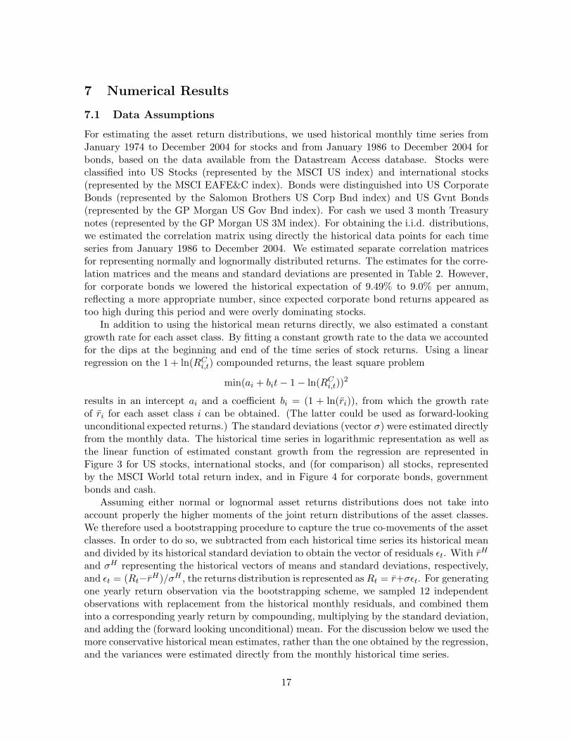
For estimating the asset return distributions, we used historical monthly time series fromJanuary 1974 to December 2004 for stocks and from January 1986 to December 2004 forbonds, based on the data available from the Datastream Access database. Stocks wereclassified into US Stocks (represented by the MSCI US index) and international stocks(represented by the MSCI EAFE&C index). Bonds were distinguished into US CorporateBonds (represented by the Salomon Brothers US Corp Bnd index) and US Gvnt Bonds(represented by the GP Morgan US Gov Bnd index). For cash we used 3 month Treasurynotes (represented by the GP Morgan US 3M index). For obtaining the i.i.d. distributions,we estimated the correlation matrix using directly the historical data points for each timeseries from January 1986 to December 2004. We estimated separate correlation matricesfor representing normally and lognormally distributed returns. The estimates for the corre-lation matrices and the means and standard deviations are presented in Table 2. However,for corporate bonds we lowered the historical expectation of 9.49% to 9.0% per annum,reflecting a more appropriate number, since expected corporate bond returns appeared astoo high during this period and were overly dominating stocks.

In addition to using the historical mean returns directly, we also estimated a constantgrowth rate for each asset class. By fitting a constant growth rate to the data we accountedfor the dips at the beginning and end of the time series of stock returns. Using a linearregression on the 1 + ln(RC

i,t) compounded returns, the least square problem

min(ai + bit − 1 − ln(RCi,t))

2

results in an intercept ai and a coefficient bi = (1 + ln(ri)), from which the growth rateof ri for each asset class i can be obtained. (The latter could be used as forward-lookingunconditional expected returns.) The standard deviations (vector σ) were estimated directlyfrom the monthly data. The historical time series in logarithmic representation as well asthe linear function of estimated constant growth from the regression are represented inFigure 3 for US stocks, international stocks, and (for comparison) all stocks, representedby the MSCI World total return index, and in Figure 4 for corporate bonds, governmentbonds and cash.

Assuming either normal or lognormal asset returns distributions does not take intoaccount properly the higher moments of the joint return distributions of the asset classes.We therefore used a bootstrapping procedure to capture the true co-movements of the assetclasses. In order to do so, we subtracted from each historical time series its historical meanand divided by its historical standard deviation to obtain the vector of residuals εt. With rH

and σH representing the historical vectors of means and standard deviations, respectively,and εt = (Rt−rH)/σH , the returns distribution is represented as Rt = r+σεt. For generatingone yearly return observation via the bootstrapping scheme, we sampled 12 independentobservations with replacement from the historical monthly residuals, and combined theminto a corresponding yearly return by compounding, multiplying by the standard deviation,and adding the (forward looking unconditional) mean. For the discussion below we used themore conservative historical mean estimates, rather than the one obtained by the regression,and the variances were estimated directly from the monthly historical time series.

17

We remark that estimating the means of stock returns, given the data at hand, may notbe very accurate. For example, our estimates for the annual means based on 374 monthlyhistorical data have an estimated standard deviation of about 2.8%. Estimates of standarddeviations and correlations are more accurate. The regression procedure provides a goodway to estimate means. The regression results for stocks, while larger than the historicalestimates, are within the confidence interval obtained for the historical mean estimates.

For the effect of estimation errors on optimal portfolio choice see, e.g., Chopra andZiemba (1993) and on turnover Chopra (1993), showing that estimation errors in the meanshave a significantly larger effect than estimation errors in the variances and covariances.Simulating estimation error by adding zero mean i.i.d normal distributions to the data, andcomparing certainty equivalent cash (wealth) in a single-period mean-variance optimizationof 10 randomly selected stocks of the Dow Jones industrial average, for a risk tolerance of50, errors in the mean estimate resulted in a 11 times larger loss of certainty equivalentcash as errors in the variances, and errors in the variances resulted in 2 times larger lossthan errors in the covariances. The effects were shown to increase with increasing risktolerance and with increasing magnitude of errors. Already earlier, Kallberg and Ziemba(1981) and (1984) concluded that errors in the mean estimate matter most. The effect oferrors in the estimates of means relative to variances and covariances on certainty equivalentwealth obviously must increase with larger risk tolerance, since at a risk tolerance of zero,where only variances and covariances enter the optimization problem, exclusively errors invariances and covariances matter, and at an infinite risk tolerance, where only means enterthe optimization problem, exclusively errors in mean estimates have an influence. Michaud(1989) showed that noisy forecasts in mean-variance optimization may lead to suboptimalportfolios, where assets with positive estimation error in the mean forecasts are significantlyover-weighted and assets with negative estimation error are significantly under-weighted inthe “optimal” portfolio, and proposed an approach based on re-sampling (bootstrapping) tocounteract this effect. As a practical approach to counter estimation error, Connor (1997)proposed for linear regression based forecasting models to use Bayesian adjusted priors toshrink mean estimates with large observed estimation errors.

A different approach for obtaining unconditional means is to use an assumed mean-variance efficient portfolio, e.g., a broad index, and to infer the unconditional means fromthe standard deviations of returns, by viewing the portfolio as the optimal solution of acorresponding mean-variance problem with an appropriate risk aversion coefficient. Thisprocedure of Grinold (1999) is called “grapes from wine”, and represents an efficient wayto calibrate mean returns. Besides estimating standard deviations based on historical timeseries, also implied volatilities based on observed option prices could be used.

7.2 An Investment Example

In order to demonstrate dynamic investment policies obtained from our dynamic portfoliochoice model, we discuss as an illustrative example a very typical investment situation. Aninvestor has a current wealth of $100k and plans to contribute $15k per year for the next20 years. What is the distribution of wealth at the end of the investment horizon, reflectingvarious reasonable assumptions about the investor’s risk aversion profile? We discuss fourcases: (A) using the CARA utility function, (B) using increasing relative risk aversion but

18

Table 2: Data Estimates for normal and log normal distributions

Historical means and standard deviations

US Stocks Int Stocks Corp Bnd Gvnt Bnd Cash

Mean 10.80 10.37 9.49 7.90 5.61STD 15.72 16.75 6.57 4.89 0.70

Regression-based means and standard deviations

US Stocks Int Stocks Corp Bnd Gvnt Bnd Cash

Mean 14.1 12.5 9.24 7.92 5.77STD 15.72 16.75 6.57 4.89 0.70

Correlation matrix for normal model

US Stocks Int Stocks Corp Bnd Gvnt Bnd Cash

US Stocks 1.00 0.601 0.247 0.062 0.094Int Stocks 0.601 1.00 0.125 0.027 0.006Corp Bnd 0.247 0.125 1.00 0.883 0.194Gvnt Bnd 0.062 0.027 0.883 1.00 0.27

Cash 0.094 0.006 0.194 0.27 1.00

Correlation matrix for log-normal model

US Stocks Int Stocks Corp Bnd Gvnt Bnd Cash

US Stocks 1.00 0.609 0.236 0.05 0.083Int Stocks 0.609 1.00 0.124 0.02 -0.002Corp Bnd 0.236 0.124 1.00 0.884 0.195Gvnt Bnd 0.05 0.02 0.884 1.00 0.271

Cash 0.083 -0.002 0.195 0.271 1.00

decreasing absolute risk aversion, (C) using decreasing relative risk aversion and decreasingabsolute risk aversion, and (D) using a quadratic penalty of under-performing a target.

For the exponential utility function (case A), we assumed an absolute risk aversioncoefficient of λ = 2. Figure 5 presents the optimal asset allocation (as a function of wealth)at various times, e.g, for one year (top), 10 years (middle) and 19 years (bottom) to go.The optimal asset allocation is not constant but varies significantly with the investmenthorizon and the wealth already accumulated. The case of one year to go is special becauseit shows the results for different wealth levels of a single-period optimization with theinvestor’s original utility function. All other period allocations represent the result forusing the implied utility function from the dynamic programming algorithm. In the lastrebalancing period, the more money that is in the investor’s account the less risk he/shetakes, and accordingly the fraction of stocks decrease with increasing account value. Whenthe account is under-performing a certain wealth level the optimal strategy prescribes toinvest entirely in stocks, where the amount to be put internationally versus domesticallyvaries with account value. This may be a significant strain on the investor, but the problemcould be corrected by using a constraint restricting the maximum exposure to stocks. If therewas no borrowing constraint, we know from analytical solutions for HARA policies that theoptimal investment would prescribe for low wealth levels to borrow funds and use this moneyto buy more than 100% stocks, thus attempting to leverage the funds available. However,this would not be practical in a low-wealth situation, since such a strategy would quicklyexceed margin requirements and thus would not be implementable. This demonstrates theimportance of considering a borrowing constraint as part of the investment problem.

19

The dependence of the optimal asset allocation on wealth changes every year, as onecan see by comparing the optimal asset allocation for only one year to go with the onesfor 10 years to go and for 19 years to go. For very high wealth levels and long remaininghorizons (e.g., 19 years to go) a small amount of cash enters the optimal portfolio. Figure 5for the optimal asset allocation strategy also displays the attainable wealth range, obtainedby simulation. The attainable range is defined by the wealth that is exceeded (left) or notexceeded (right) with 99.9% probability, respectively. For example, in year 19 the attainablerange is between $0.55 and $3.21 million, in year 10 between $0.25 and $0.89 million, andin year 1 (after the first year of investment) between $0.09 and $0.17 million, including thecash flow at the beginnning of the period.

Figure 6 (top) represents the expected value strategy, i.e., the optimal investment strat-egy implemented over time, assuming every year that the expected returns would be real-ized. At (the current) period zero, the optimal portfolio is 54% US stocks, 17% internationalstocks, and 29% corporate bonds. Cash and government bonds are not part of the initialportfolio. One can observe that from the optimal allocation at the outset of approximately71% stocks and 29% bonds, the allocation changes gradually to approximately 37% stocksand 63% bonds at year 19, when the last portfolio decision is to be made. This path issimilar to strategies that investment firms tend to prescribe their clients and recently havebeen implemented as life-cycle funds. The reasoning behind such strategies is to reducestock allocation as the investment horizon shortens to prevent a possible significant losswithout a good prospect of recovery before the end of the investment horizon. However, thestrategies of practitioners and life-cycle funds are different to our dynamic strategy in thatthey do not react to prior performance. We can also view the dynamic strategy by startingfrom the expected value path, where stock allocation and risk is reduced as the remaininginvestment horizon shortens. In each period the stock allocation and the risk is reduced ifthe performance was better than expected (and thus the available wealth is larger), and thestock allocation and the risk is increased if the performance was worse than expected (andthus the wealth is smaller).

Figure 6 depicts (in the middle) the out-of-sample simulations of wealth over time and(at the bottom) the resulting marginal distribution of wealth at the end of the investmenthorizon. Table 3 summarizes the statistics of wealth obtained at the end of the investmenthorizon. The mean wealth is $1.564 million, with a standard deviation of $0.424 million.With 99% probability a wealth of $770,000 is exceeded and with 95% probability a wealthof $943,000. The certainty equivalent wealth is $1.412 million.

Alleged shortcomings of the exponential utility function (constant absolute risk aversion)include that very high stock allocations at very low wealth levels may lead to a too-high riskburden on the investor, and a too-small relative risk aversion at very high wealth levels maylead to overly conservative asset allocations. While both shortcomings can be compensatedfor with lower and upper bounds on the stock allocation, another way is to model the properrisk aversion of the investor directly.

For the increasing relative risk aversion utility function (case B), we assumed that at awealth below WL = 0.25, the relative risk aversion is γ = 2, increasing linearly with wealthto γ = 3.5 at a wealth of WU = 3.5 and then remaining at that level for larger wealth levels.This profile of relative risk aversion was modeled using the piecewise exponential utilityrepresentation discussed above, using 200 exponential (CARA) pieces between WL and WU ,

20

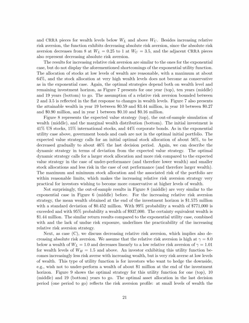
and CRRA pieces for wealth levels below WL and above WU . Besides increasing relativerisk aversion, the function exhibits decreasing absolute risk aversion, since the absolute riskaversion decreases from 8 at WL = 0.25 to 1 at WU = 3.5, and the adjacent CRRA piecesalso represent decreasing absolute risk aversion.

The results for increasing relative risk aversion are similar to the ones for the exponentialcase, but do not display the aforementioned shortcomings of the exponential utility function.The allocation of stocks at low levels of wealth are reasonable, with a maximum at about64%, and the stock allocation at very high wealth levels does not become as conservativeas in the exponential case. Again, the optimal strategies depend both on wealth level andremaining investment horizon, as Figure 7 presents for one year (top), ten years (middle)and 19 years (bottom) to go. The assumption of a relative risk aversion bounded between2 and 3.5 is reflected in the flat response to changes in wealth levels. Figure 7 also presentsthe attainable wealth in year 19 between $0.59 and $3.44 million, in year 10 between $0.27and $0.90 million, and in year 1 between $0.10 and $0.16 million.

Figure 8 represents the expected value strategy (top), the out-of-sample simulation ofwealth (middle), and the marginal wealth distribution (bottom). The initial investment is41% US stocks, 15% international stocks, and 44% corporate bonds. As in the exponentialutility case above, government bonds and cash are not in the optimal initial portfolio. Theexpected value strategy calls for an initial optimal stock allocation of about 56%, to bedecreased gradually to about 46% the last decision period. Again, we can describe thedynamic strategy in terms of deviation from the expected value strategy. The optimaldynamic strategy calls for a larger stock allocation and more risk compared to the expectedvalue strategy in the case of under-performance (and therefore lower wealth) and smallerstock allocations and less risk in the case of out performance (and therefore larger wealth).The maximum and minimum stock allocation and the associated risk of the portfolio arewithin reasonable limits, which makes the increasing relative risk aversion strategy verypractical for investors wishing to become more conservative at higher levels of wealth.

Not surprisingly, the out-of-sample results in Figure 8 (middle) are very similar to theexponential case in Figure 6 (middle) before. For the increasing relative risk aversionstrategy, the mean wealth obtained at the end of the investment horizon is $1.575 millionwith a standard deviation of $0.452 million. With 99% probability a wealth of $771,000 isexceeded and with 95% probability a wealth of $937,000. The certainty equivalent wealth is$1.44 million. The similar return results compared to the exponential utility case, combinedwith and the lack of undue risk exposure, underlines the practicability of the increasingrelative risk aversion strategy.

Next, as case (C), we discuss decreasing relative risk aversion, which implies also de-creasing absolute risk aversion. We assume that the relative risk aversion is high at γ = 8.0below a wealth of WL = 1.0 and decreases linearly to a low relative risk aversion of γ = 1.01for wealth levels of WH = 1.5 and above. An investor exhibiting this utility function be-comes increasingly less risk averse with increasing wealth, but is very risk averse at low levelsof wealth. This type of utility function is for investors who want to hedge the downside,e.g., wish not to under-perform a wealth of about $1 million at the end of the investmenthorizon. Figure 9 shows the optimal strategy for this utility function for one (top), 10(middle) and 19 (bottom) years to go. The optimal asset allocation in the last decisionperiod (one period to go) reflects the risk aversion profile: at small levels of wealth the

21

stock allocation is small at about 21% and increases to about 87% stocks at higher levelsof wealth. Again, the asset allocation changes with the remaining investment horizon andwealth, where the point of low stock allocations shifts towards higher wealth levels as theremaining investment horizon decreases and the change of allocation becomes less gradual.We also observe very conservative investments at very low wealth levels, but these are outof the range of wealth that can be reasonably obtained. The initial portfolio is 11% USstocks, 10% international stocks, 60% corporate bonds, and 19% government bonds. Cashis not part of the initial portfolio. The expected value strategy in Figure 10 (top) showsthat the stock allocation and thus the risk increases with time starting from about 21%stocks at the initial investment up to 50% stocks at the last decision period in year 19.This reflects the investor’s profile as a time path, where he/she is careful at low levels ofwealth, but becomes increasingly less risk averse as wealth grows over time. Relative to theexpected value path, the strategy prescribes in each period to increase the stock allocationand the risk if the performance was better than expected (and more wealth than expectedis available) and to reduce the stock allocation and risk if under-performance occurred (andless wealth than expected is available). Figure 9 presents the attainable wealth in year 19between $0.71 and $3.75 million, in year 10 between $ 0.29 and $0.80 million, and in year1 between $0.11 and $0.15 million.

Figure 10 (in the middle) gives the out-of-sample simulation results, and (at the bottom)the marginal distribution of terminal wealth. In both views, one can observe that thedownside is more protected than in the previous cases. The mean wealth obtained at theend of the investment horizon is $1.498 million with a standard deviation of $0.436 million.With 99% probability a wealth of $866,000 is exceeded and with 95% probability a wealthof $998,000. These are reasonable out-of-sample results for an investor wishing to protecthis/her downside below $1 million. The certainty equivalent wealth is $1.339 million (Table3).

The optimal dynamic strategies for increasing and decreasing relative risk aversion be-have in a mirrored way. Assuming a crash in the stock market occurred, we can deducethat an investor with increasing relative risk aversion would react by increasing the stockallocation in order to make up for the loss, while the investor with decreasing relative riskaversion would reduce his/her stock allocation in order to further protect the downside. Andwe know that an investor with constant relative risk aversion (CRRA) would re-balance afterthe crash back to his/her original asset allocation. We may use this theoretical behavior tohelp infer the type of utility function that is most appropriate for an investor.

Case (D) reflects risk as a quadratic penalty of under-performing a target wealth. Weassumed a target wealth of $1M and traded off risk and expected return using a risk aversionof λq/2 = 1000. This is an extreme case reflecting an investor wishing to obtain a wealthof $1 million very badly and therefore being prepared to forsake a significant part of theupside. Figure 11 presents the dynamic investment strategy for one (top), ten (middle)and 19 (bottom) years to go. Looking at the last rebalancing period, the optimal strategyreflects an increasing stock allocation for higher levels of wealth, starting slightly belowthe target wealth. This “critical” wealth level is where the target can still be reachedwith very high probability. Reducing wealth from large values, the closer we are to thiscritical wealth level, the more conservative the investment becomes, up to putting almostthe entire portfolio into cash. For wealth levels above the target, stock allocations increase

22

with increasing wealth up to 100%. For wealth levels below the critical level, the strategybecomes more risky with decreasing wealth, with stock allocations also rising up to 100%.This behavior reflects exactly the risk aversion represented by the quadratic downside utilityfunction. For wealth levels above the target, the linear term (representing zero risk aversion)is dominant and leads to increased stock allocations up to 100 percent. For wealth levelsbelow the critical point, the quadratic part of the utility function is dominant. Penalizingunder-performance quadratically leads to a relative risk aversion that decreases with largerunder-performance and thus increases with larger wealth. Therefore, the quadratic utilityfunction reflects increasing relative risk aversion below the critical wealth and decreasingrelative risk aversion above. With longer remaining investment horizons the critical pointof reaching the target shifts to the left, and the allocation at that point becomes lessconservative. With ten years to go, the critical wealth level is at about $0.58 million andthe allocation is at about 65% cash. Interestingly, with 19 years to go, the reachable wealthlevels are all below the critical point and the strategy is entirely one of decreasing relativerisk aversion, calling for stock allocations from about 60% at low levels of wealth following abad first year to 30% after an out-performing first year. Figure 11 represents the attainablewealth in year 19 between $0.72 and $3.40 million, in year 10 between $0.29 and $0.71million, and in year 1 between $0.10 and $0.16 million.

The initial portfolio is 36% US stocks, 14% international stocks, and 50% corporatebonds. Government bonds and cash are not part of the initial optimal portfolio. Theexpected return strategy in Figure 12 (top) confirms this result. Starting at an initialstock allocation of 50%, the stock allocation is reduced gradually through year 13 and thenincreased from year 14 on. Given the savings rate and the results from the investments,the investor first starts in an under-performing state, then achieves the critical wealth levelduring year 14, and ends above the critical wealth.

The out-of-sample simulation results in Figure 12 (middle) show good downside pro-tection and the marginal probability chart (bottom) is very steep on the left reflecting thedownside protection the quadratic downside risk function is said to provide. However, eventhe assumption of a very large risk aversion coefficient does not lead to a zero probability ofwealth below $1 million. The mean wealth obtained at the end of the investment horizon is$1.339 million with a standard deviation of $0.347 million. With 99% probability a wealthof $911,000 is exceeded and with 95% probability a wealth of $1.006 million. Thus, thetarget wealth of $1 million is exceeded with larger than 95% probability. The statistics inTable 3 give a certainty equivalent wealth of $998.000 as the lowest of all four utility func-tions, reflecting again the low emphasis on the upside displayed by the quadratic downsideutility function.

7.3 The Performance of Dynamic Strategies

Next we compare dynamic strategies obtained from using the different utility functions witha number of fixed-mix strategies, i.e., (1) US stocks only, (2) cash only, (3) all asset classesequally weighted, (4) risk averse, (5) medium, and (6) risk prone. Except for case (3), allfixed-mix strategies are mean-variance efficient and obtained from solving the single-periodMarkowitz problem. Figure 2 presents the efficient frontier and the efficient fixed-mixportfolios. We intentionally use the five representative mean-variance optimal fixed-mix

23

Table 3: Out-of-sample simulation results

CEW Mean Std 99% 95%

Exponential RA=2 1.412 1.564 0.424 0.770 0.943

Increasing RRA 1.440 1.575 0.452 0.771 0.937

Decreasing RRA 1.339 1.498 0.436 0.865 0.998

Quadratic 0.982 1.339 0.347 0.911 1.006

downside 1.349 1.481 0.352 0.865 0.997

strategies for comparison, because such portfolios are commonly held in practice. Manyaggressive investors hold stocks-only portfolios, and many very conservative investors keeptheir funds entirely in money market accounts. Investment firms usually offer fund-of-fundsportfolios, such as averse (often called conservative), medium (often referred to as dynamic),and prone (often referred to as aggressive), which are sold to investors allegedly accordingto their risk profile. The equally weighted strategy represents a non-efficient portfolio forcomparison.

Efficient Frontier

US Stocks

ProneMedium

Averse

Cash only

0

2

4

6

8

10

12

0 2 4 6 8 10 12 14 16 18

Risk (Std) (% p.a.)

Ecpe

cted

Ret

urn

(% p

.a.)

Figure 2: Efficient frontier and efficient portfolios for fixed-mix strategies

Table 4 represents the out-of-sample simulation results for the various fixed-mix strate-gies. Obviously, the largest expected wealth of $1.825 million is obtained by the US Stocksportfolio, and the smallest expected wealth of $0.868 million by the cash-only portfolio.More interestingly, the cash-only portfolio exceeds a wealth of $822,000 with 99% proba-bility, and the medium portfolio exceeds a wealth of $825,000 with 99% probability. Theexpected wealth of the cash-only portfolio is a mere $868,000 compared to the expectedwealth of the medium portfolio of $1.538 million.

24

The risk-averse strategy exhibits the largest wealth of $869,000 exceeded with 99%probability, with an expected wealth of $ 1.098 million at the end of the investment horizon.In comparison, the dynamic strategy of decreasing relative risk aversion exhibits a verysimilar wealth of $865,000 exceeded with 99% probability, but a significantly larger expectedwealth of $1.339 million. This represents an increase of 21.95% expected wealth at thesame level of (downside) risk. The medium strategy exhibits the largest wealth of $975,000exceeded with 95% probability among all fixed-mix strategies. The best dynamic strategyon this measure is the quadratic downside risk strategy, which exceeds $1.006 million with95% probability. However, the quadratic strategy returns a significantly lower expectedwealth of $1.339 million, compared with 1.538 million for the medium fixed-mix strategy.The extra downside protection is expensive on the upside. There is no dynamic strategymatching the 95% exceeded wealth of the medium fixed-mix strategy, and therefore wecannot make a statement of out-performance at the same level of 95% exceeded wealthgiven the strategies at hand.

Table 4: Out-of-sample simulation results for various fixed-mix strategies

Mean Std 99% 95%

US Stocks 1.825 1.065 0.469 0.660

Cash 0.868 0.019 0.822 0.834

Equally weighted 1.349 0.301 0.799 0.920

Averse 1.098 0.110 0.869 0.930

Medium 1.538 0.407 0.825 0.975

Prone 1.663 0.639 0.677 0.852

In order to further evaluate the dynamic strategies, we compared the certainty equiva-lent wealth (CEW) of the dynamic strategies with the corresponding certainty equivalentwealth of each fixed-mix strategy. Table 5 presents the results in terms of certainty equiva-lent wealth and in the percentage improvement obtained when using the optimal dynamicstrategy for each utility function compared to each of the fixed-mix strategies.

A certainty equivalent wealth (CEW) of $1.41193 million is the maximum obtained froma dynamic strategy in the case of the exponential utility function with risk aversion of λ = 2.This utility represents a fairly aggressive investor. The medium strategy would be the bestfixed-mix strategy with an CEW of $1.40415 million. The improvement of the dynamicstrategy versus the best fixed-mix strategy is 0.55%. The prone strategy would also fitreasonably well this investor, and results in a CEW of $1.38933 million. The improvementof the dynamic strategy versus the prone strategy is 1.63%. The improvements in CEWof the dynamic strategy versus US stocks, cash and averse are 9.61%, 62.79% and 29.93%,respectively.

Not surprisingly, the situation is very similar for the increasing relative risk aversionutility function. The dynamic strategy results in a certainty equivalent wealth of $1.44004million. The prone strategy is the best fixed-mix strategy with a CEW of $1.43378 million,resulting in an improvement of the dynamic strategy versus prone of 0.44%. The mediumstrategy is surpassed by the dynamic strategy by 0.76%. US stocks, cash only and riskaverse are surpassed by the dynamic strategy by 7.17%, 66.04% and 32.42%, respectively.

25

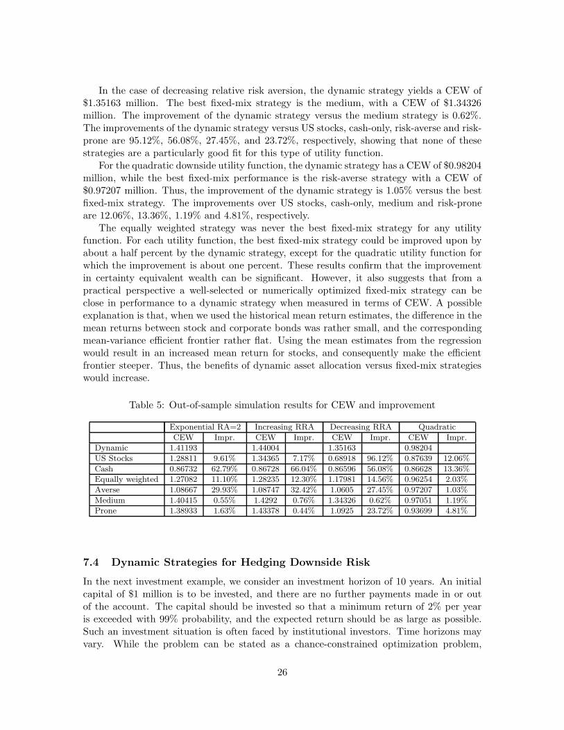
In the case of decreasing relative risk aversion, the dynamic strategy yields a CEW of$1.35163 million. The best fixed-mix strategy is the medium, with a CEW of $1.34326million. The improvement of the dynamic strategy versus the medium strategy is 0.62%.The improvements of the dynamic strategy versus US stocks, cash-only, risk-averse and risk-prone are 95.12%, 56.08%, 27.45%, and 23.72%, respectively, showing that none of thesestrategies are a particularly good fit for this type of utility function.

For the quadratic downside utility function, the dynamic strategy has a CEW of $0.98204million, while the best fixed-mix performance is the risk-averse strategy with a CEW of$0.97207 million. Thus, the improvement of the dynamic strategy is 1.05% versus the bestfixed-mix strategy. The improvements over US stocks, cash-only, medium and risk-proneare 12.06%, 13.36%, 1.19% and 4.81%, respectively.

The equally weighted strategy was never the best fixed-mix strategy for any utilityfunction. For each utility function, the best fixed-mix strategy could be improved upon byabout a half percent by the dynamic strategy, except for the quadratic utility function forwhich the improvement is about one percent. These results confirm that the improvementin certainty equivalent wealth can be significant. However, it also suggests that from apractical perspective a well-selected or numerically optimized fixed-mix strategy can beclose in performance to a dynamic strategy when measured in terms of CEW. A possibleexplanation is that, when we used the historical mean return estimates, the difference in themean returns between stock and corporate bonds was rather small, and the correspondingmean-variance efficient frontier rather flat. Using the mean estimates from the regressionwould result in an increased mean return for stocks, and consequently make the efficientfrontier steeper. Thus, the benefits of dynamic asset allocation versus fixed-mix strategieswould increase.

Table 5: Out-of-sample simulation results for CEW and improvement

Exponential RA=2 Increasing RRA Decreasing RRA Quadratic

CEW Impr. CEW Impr. CEW Impr. CEW Impr.

Dynamic 1.41193 1.44004 1.35163 0.98204

US Stocks 1.28811 9.61% 1.34365 7.17% 0.68918 96.12% 0.87639 12.06%

Cash 0.86732 62.79% 0.86728 66.04% 0.86596 56.08% 0.86628 13.36%

Equally weighted 1.27082 11.10% 1.28235 12.30% 1.17981 14.56% 0.96254 2.03%

Averse 1.08667 29.93% 1.08747 32.42% 1.0605 27.45% 0.97207 1.03%

Medium 1.40415 0.55% 1.4292 0.76% 1.34326 0.62% 0.97051 1.19%

Prone 1.38933 1.63% 1.43378 0.44% 1.0925 23.72% 0.93699 4.81%

7.4 Dynamic Strategies for Hedging Downside Risk

In the next investment example, we consider an investment horizon of 10 years. An initialcapital of $1 million is to be invested, and there are no further payments made in or outof the account. The capital should be invested so that a minimum return of 2% per yearis exceeded with 99% probability, and the expected return should be as large as possible.Such an investment situation is often faced by institutional investors. Time horizons mayvary. While the problem can be stated as a chance-constrained optimization problem,

26

we will explore empirically whether downside risk protection can be achieved by utilitymaximization using the quadratic downside risk or the decreasing relative risk aversionutility function.

For the quadratic function we set the target wealth at $1.22 milion reflecting the 2% peryear minimum return to be exceeded with 99% probability. As in the investment exampleabove, we set the risk aversion at λq/2 = 1000, in order to heavily penalize any under-performance with respect to the target. For the decreasing relative risk aversion function,we set a high relative risk aversion of γ = 8 below the level WL = $1.22 million (the targetwealth) and a low relative risk aversion of γ = 1.01 above the wealth level WH = $1.5million, and assume the relative risk aversion increases linearly in between. For both utilityfunctions, we solved the 10-year horizon problem assuming yearly, quarterly and monthlyrebalancing. For quarterly rebalancing a 40-stage problem needed to be solved, and for themonthly rebalancing a 120-stage problem.

Table 6 gives the results for expected wealth, wealth exceeded with 99% probability, andminimum wealth (defined as the level exceeded with 99.9% probability), as well as expectedreturn, return exceeded with 99% probability and minimum return (exceeded with 99.9%probability). Using yearly rebalancing, both utility functions lead to larger returns than2% per annum with at least 99% probability. The quadratic downside utility function re-sulted in a very conservative strategy, and even the minimum returns (exceeded with 99.9%probability) met the 2% per year requirement. The expected returns from both strategiesare 10.35% per year for the quadratic downside and 10.42% for the decreasing RRA util-ity function, indicating that the downside-risk-protected strategies are not overly costly onthe upside. The results were rather similar for yearly, quarterly and monthly rebalancingfor both utility functions; however, more frequent rebalancing allowed for somewhat betterdownside protection and larger expected returns.

Table 6: Out-of-sample simulation results for downside risk protection

Rebal. Periods Exp Wealth 99% Wealth Min Wealth Exp Ret. 99% Ret. Min Ret.

Quadratic downside risk

yearly 10 2.67628 1.31957 1.22778 10.35% 2.81% 2.07%quarterly 40 2.79864 1.28774 1.22500 10.84% 2.56% 2.05%monthly 120 2.71229 1.36413 1.26250 10.49% 3.15% 2.36%

Decreasing RRA

yearly 10 2.69504 1.25000 1.10000 10.42% 2.26% 0.96%quarterly 40 2.78378 1.26714 1.05000 10.78% 2.40% 0.49%monthly 120 2.76007 1.32083 1.10000 10.69% 2.82% 0.96%

For the quadratic downside risk strategy, Figure 13 represents the optimal asset allo-cation for yearly rebalancing with respect to wealth for one (top), five (middle) and nineyears to go. For all attainable wealth levels (achieved with 99.9% probability), the optimalasset allocation is entirely on the right side of the critical wealth (with the most conserv-ative asset allocation) and thus exhibits decreasing relative risk aversion. The better theperformance (and the larger the wealth in the account), the more risk should be assumedand the larger should be the stock allocation. The attainable wealth in year 9 lies between$1.16 and $7.35 million, in year 5 between $0.96 and $3.54 million, and in year 1 between

27

$0.80 and $1.41 million. Figure 14 (top) represents the expected value strategy (assumingexpected returns are realized in every period), (middle) the simulations of wealth over time,and (bottom) the marginal distribution of wealth at the end of the investment horizon foryearly rebalancing. The expected value strategy prescribes to start with an initial assetallocation of 60% stocks and 40% corporate bonds, and then to gradually increase the stockallocation to almost 100% in the last rebalancing period. The marginal distribution is steepon the left side, representing a limited downside, and the minimum wealth (exceeded with99.9%) of $1.22778 million translates into a minimal annual return of 2.07%.

How well this strategy protects the downside along the way is presented in Table 7, whichexhibits the expected wealth, the wealth exceeded with 99% probability, and the minimumwealth (that is exceeded with 99.9% probability), along with corresponding measures for thereturns in each year of the investment horizon. The downside protection during the initialperiods is rather weak, with the returns exceeded with 99% probability in year one resultingas -11.86% and the minimum return resulting as -20.00%. Only in year five is nominal capitalpreserved with greater than 99% probability and only in year six with 99.9% probability.In year eight the target return of 2% per year is exceeded with 99% probability, and in year10 with 99.9% probability. The expected returns increase monotonically as time passes, butonly marginally from 10.01% per year in year one to 10.35% in year ten.

Table 7: Out-of-sample simulation results for downside risk protection

Quadratic dynamic downside risk

Period Exp Wealth 99% Wealth Min Wealth Exp Ret. 99% Ret. Min Ret.

1 1.10008 0.8814 0.8 10.01% -11.86% -20.00%2 1.21161 0.89267 0.825 10.07% -5.52% -9.17%3 1.33354 0.92828 0.86 10.07% -2.45% -4.90%4 1.47004 0.97231 0.9 10.11% -0.70% -2.60%5 1.62245 1.01714 0.9616 10.16% 0.34% -0.78%6 1.79528 1.07636 1 10.24% 1.23% 0.00%7 1.98402 1.1296 1.05333 10.28% 1.76% 0.74%8 2.19368 1.18286 1.12 10.32% 2.12% 1.43%9 2.42128 1.25091 1.16071 10.32% 2.52% 1.67%10 2.67628 1.31957 1.22778 10.35% 2.81% 2.07%

We next compare these results to the results of a strategy where the downside is con-trolled dynamically in every period.

7.5 Downside Risk Protection at Every Period

Especially institutional investors are evaluated with regard to their portfolio’s performanceon a yearly basis. Given the ongoing evaluations, institutional managers may considerimplementing a dynamic strategy with limited downside risk not only at the end of theinvestment horizon but also at every year along the way. Again, using a 10-year investmenthorizon, we compute a strategy using a discounted additive quadratic downside utilityfunction at every year. For the dynamic quadratic downside risk utility function, the dis-count factor was chosen as 1% per year and the target wealth in each period was set asWd,t = 1.02t, t = 1, 10 reflecting the desired minimum return of 2% per year. We set the

28

risk aversion coefficient at every period as λl = 1000 and λq/2 = 1000, in order to heavilypenalize (linearly and quadratically) any under-performance with respect to the targets inaddition to the quadratic downside utility function at the end of the investment horizon.

Figure 15 represents the strategies for one (top), five (middle) and nine (bottom) yearsto go. The optimal strategy at the last rebalancing period must be identical to that, whereonly terminal wealth is evaluated. This follows directly from the dynamic programmingrecursion. At all other years the dynamically controlled downside risk strategy is moreconservative, e.g., at five years to go risk and stock allocation increases slower with wealthcompared to the uncontrolled case (with downside risk protection only at the end of theinvestment horizon), and the most conservative allocation at the critical point is moreconservative than in the uncontrolled case. For example, in the uncontrolled case at nineyears to go, the cash position at the critical point is about 70%, whereas in the controlledcase it is about 90%. With downside controls, the attainable wealth in year 9 lies between$1.26 and $5.36 million, in year 5 between $1.13 and $2.30 million, and in year 1 between$1.01 and $1.12 million. This is more narrow range than for the uncontrolled case, reflectingthe loss on the upside induced by the protection on the downside.

Figure 16 (top) represents the expected value strategy, (middle) the simulations ofwealth, and (bottom) the marginal probability distribution of terminal wealth. The ex-pected value strategy under downside control prescribes to start with a stock allocation of5% and to increase it up to about 85% in year nine. This is significantly more conservativethan in the uncontrolled case. Comparing the wealth simulations, one can readily observethat the downside is more protected along the way than in the uncontrolled case.

Table 8: Out-of-sample simulation results for dynamic downside risk protection at everyperiod

Quadratic dynamic downside risk

Period Exp Wealth 99% Wealth Min Wealth Exp Ret. 99% Ret. Min Ret.

1 1.06575 1.02225 1.00533 6.58% 2.23% 0.53%2 1.14561 1.06108 1.032 7.03% 3.01% 1.59%3 1.24271 1.09137 1.06222 7.51% 2.96% 2.03%4 1.35621 1.13641 1.095 7.91% 3.25% 2.29%5 1.48549 1.176 1.12667 8.24% 3.30% 2.41%6 1.63401 1.22638 1.152 8.53% 3.46% 2.39%7 1.79975 1.27385 1.2 8.76% 3.52% 2.64%8 1.9845 1.32121 1.23 8.94% 3.54% 2.62%9 2.18661 1.37778 1.26 9.08% 3.62% 2.60%10 2.41527 1.43966 1.3125 9.22% 3.71% 2.76%

Table 8 presents the statistics for each year of the investment horizon. (The last lineof year 10 represents the terminal statistics.) The marginal distribution of final wealthdisplays a minimum wealth (exceeded with 99.9% probability) of $1.3125 million, whichtranslates into a 2.76% annual return. Compared to the uncontrolled case above, thedownside is much better protected along the way, e.g., in every period the return exceededwith 99% probability is greater than 2%, and the minimum return (exceeded with 99.9%probability) exceeds 2% from year three on. The expected return is smaller compared to

29

the unconstrained case and increases monotonically from 6.58% to 9.22%, which confirmsthat the dynamically downside-controlled strategy is overall more conservative than whenonly the terminal distribution is considered in the optimization.

These are very encouraging results. All out-of-sample simulations were performed usingbootstrapping from the historical monthly observations and thus represent possible fat tailsin the asset returns distribution.

7.6 Computation Times

For the optimization we used a sample size of |Sit| = 2000 of annual returns for each period.

The sample is based on bootstrapping from the monthly returns, thus we used 24,000sampled monthly observations to compute the annual returns sample. In each period forthe out-of-sample evaluation, we used a sample size of |So

t | = 5000 of annual returns, alsoobtained by bootstrapping monthly returns. The computations were carried out usingthe fast method, pre-calculating the efficient frontier parameterized at 2000 points. Aftercomputing the optimal strategy, we simulated 5000 paths based on bootstrapping monthlyreturns. The following Table 9 presents the optimization time in CPU seconds (on a Pentium4 3.4 MHz and 2GB of RAM) for the different time horizons and utility functions used. Ittakes about 11 seconds to optimize a 20-period problem with yearly rebalancing, thus solvinga 20-stage stochastic dynamic program. The computation time was about 8 seconds for a10-year horizon with yearly rebalancing, about 17 seconds for quarterly rebalancing and 41seconds for monthly rebalancing. In the latter, a 120 stage stochastic dynamic program wassolved in 41 seconds.

The fast computations for yearly rebalancing permit us to carry out the calculationson-line. We have developed a commercial system, called WealthiOR, to help investmentadvisors find the best asset allocation strategies for their clients, individual and institutional.The system is web-based and the optimizations and simulations are carried out on-line inreal time. The system is user friendly, easy to use, and also facilitates graphical outputand downloadable tables for spreadsheets, providing all necessary statistical information. Itpermits an adviser to quickly devise customized (regarding risk preference and time horizon)optimized forward-looking dynamic strategies.

Table 9: Computation times in elapsed CPU seconds

Rebalancing Horizon Periods Utility

Exponential Increasing RRA

yearly 20 20 10.53 10.92

Quadratic Decreasing RRA

yearly 20 20 10.48 11.81

Quadratic Decreasing RRA

yearly 10 10 6.58 7.79quarterly 10 40 15.85 17.06monthly 10 120 41.35 41.35

30

8 Comparison to Multi-Stage Stochastic Programming

Our results demonstrate that, using the stochastic dynamic programming approach, assetallocation problems with many asset classes and many time periods can be solved efficientlyand accurately, allowing for a detailed discussion of the resulting investment strategies. Theapproach can also handle options and serial dependency of asset returns modeled by re-stricted autoregressive processes using a small number of predictors. Also, stochastic cashflows to represent uncertain liabilities can be handled by the approach to the extent thatthe serial correlation of the joint probability distribution of asset returns and cash flowscan be modeled with a small number of state variables. This makes the approach alsoapplicable to classes of the more general asset-liability problem. From a statistical perspec-tive (considering the historical data available for estimating the processes and the numberof parameters that need to be estimated), predictions based on too many autoregressivefactors may lead to over-fitting, resulting in weak out-of-sample performance. Thus, froma practical perspective, predictions based on a limited number of factors (state variables)seem adequate, and thus the stochastic dynamic programming approach can be efficientlyemployed for solving a wide class of practical problems.

For general returns processes with many predictive variables, and when transaction costsmust be considered, multi-stage stochastic programming can be employed successfully. Forexample, Collomb and Infanger (2005) explored the impact of serial correlation in assetreturns on the optimal asset allocation strategy. The focus of the study was on activeportfolio management on the asset class level in a multi-period look-ahead setting. Forrepresenting serial correlation, we estimated a lag-one vector autoregressive process forstocks, bonds and cash, and formulated a four-stage stochastic linear program representingthe dynamic asset allocation problem for three annual periods of look-ahead. Modelingthe stochastic program, a typical scenario tree was represented by (50 × 50 × 40) scenariosleading to 100,000 scenarios, and the corresponding deterministic equivalent formulation ofthe stochastic program had several hundred thousand rows and columns. Such problemswere typically solved in about 2 hours CPU time as deterministic equivalent linear programsand in about 20 minutes when solved using decomposition as implemented in Infanger’s(1997) DECIS code. In comparison, the stochastic dynamic programming recursion with2000 scenarios per period and 10 periods look ahead took only about 10 seconds.

Acknowledgements

The author wishes to thank Peter Glynn, John Stone, and the editors, William Ziemba andStavros Zenios, for their editorial suggestions on previous versions of this paper.

31

Historical Performance Nominal

0

0.5

1

1.5

2

2.5

3

3.5

4

4.5

5

0 60 120 180 240 300 360 420

Month (1 = Jan 1974, 384 = DEC 2004)

1 +

Log

Val

ue o

f Ass

et

US_Stocks Regression

Historical Performance Nominal

0

0.5

1

1.5

2

2.5

3

3.5

4

4.5

5

0 60 120 180 240 300 360 420

Month (1 = Jan 1974, 384 = DEC 2004)

1 +

Log

Val

ue o

f Ass

et

Int_Stocks Regression

Historical Performance Nominal

0

0.5

1

1.5

2

2.5

3

3.5

4

4.5

5

0 60 120 180 240 300 360 420

Month (1 = Jan 1974, 384 = DEC 2004)

1 +

Log

Val

ue o

f Ass

et

All_Stocks Regression

Figure 3: Monthly stock performance, January 1974 — December 2004 (US stocks, inter-national stocks, whole world)

32

Historical Performance Nominal

0

0.5

1

1.5

2

2.5

3

0 60 120 180 240

Month (1 = Jan1986, 228 = Dec 2004)

1 +

Log

Val

ue o

f Ass

et

Gvnt_Bnd Regression

Historical Performance Nominal

0

0.5

1

1.5

2

2.5

3

0 60 120 180 240

Month (1 = Jan1986, 228 = Dec 2004)

1 +

Log

Val

ue o

f Ass

et

Corp_Bnd Regression

Historical Performance Nominal

0

0.5

1

1.5

2

2.5

0 60 120 180 240

Month (1 = Jan1986, 228 = Dec 2004)

1 +

Log

Val

ue o

f Ass

et

Cash Regression

Figure 4: Monthly bond performance, January 1986 — December 2004 (corporate bonds,government bonds, cash)

33

Optimal Asset Allocation

0.00

0.10

0.20

0.30

0.40

0.50

0.60

0.70

0.80

0.90

1.00

0.02

0.08

0.14

0.20

0.26

0.32

0.38

0.44

0.50

0.56

0.62

0.68

0.74

0.80

0.86

0.92

0.98

1.04

1.10

1.16

1.22

1.28

1.34

1.40

1.46

1.52

1.58

1.64

1.70

1.76

1.82

1.88

1.94

2.00

Wealth

Frac

tion

of A

sset

s

USStox IntStox CorpBnd GvmtBnd Cash

Year 19 1 years to go

Attainable Range: 0.55 - 3.21

Optimal Asset Allocation

0.00

0.10

0.20

0.30

0.40

0.50

0.60

0.70

0.80

0.90

1.00

0.01

0.04

0.07

0.10

0.13

0.16

0.19

0.22

0.25

0.28

0.31

0.34

0.37

0.40

0.43

0.46

0.49

0.52

0.55

0.58

0.61

0.64

0.67

0.70

0.73

0.76

0.79

0.82

0.85

0.88

0.91

0.94

0.97

1.00

Wealth

Frac

tion

of A

sset

s

USStox IntStox CorpBnd GvmtBnd Cash

Year 10 10 years to go

Attainable Range: 0.25 - 0.89

Optimal Asset Allocation

0.00

0.10

0.20

0.30

0.40

0.50

0.60

0.70

0.80

0.90

1.00

0.00

0.01

0.01

0.02

0.03

0.03

0.04

0.04

0.05

0.06

0.06

0.07

0.07

0.08

0.09

0.09

0.10

0.10

0.11

0.12

0.12

0.13

0.13

0.14

0.15

0.15

0.16

0.16

0.17

0.18

0.18

0.19

0.19

0.20

Wealth

Frac

tion

of A

sset

s

USStox IntStox CorpBnd GvmtBnd Cash

Year 1 19 years to go

Attainable Range: 0.09 - 0.17

Figure 5: Investment example: initial $100k plus $15k per year, 20-year horizon: exponentialutility, investment strategy

34

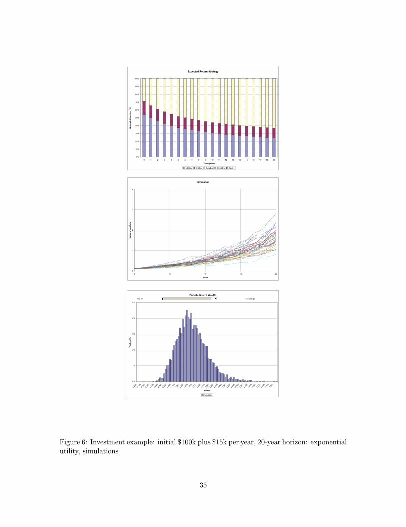
Expected Return Strategy

0%

10%

20%

30%

40%

50%

60%

70%

80%

90%

100%

0 1 2 3 4 5 6 7 8 9 10 11 12 13 14 15 16 17 18 19

Time (years)

Opt

imal

Allo

catio

n (%

)

USStox IntStox CorpBnd GvmtBnd Cash

Simulation

0

1

2

3

4

0 5 10 15 20

Years

Val

ue o

f por

tfol

io

Distribution of Wealth

0%

1%

2%

3%

4%

5%

0.040

0.160

0.280

0.400

0.520

0.640

0.760

0.880

1.000

1.120

1.240

1.360

1.480

1.600

1.720

1.840

1.960

2.080

2.200

2.320

2.440

2.560

2.680

2.800

2.920

3.040

3.160

3.280

3.400

3.520

3.640

3.760

3.880

Wealth

Pro

babi

lity

Probability

Year 20 0 years to go

Figure 6: Investment example: initial $100k plus $15k per year, 20-year horizon: exponentialutility, simulations

35

Optimal Asset Allocation

0.00

0.10

0.20

0.30

0.40

0.50

0.60

0.70

0.80

0.90

1.00

0.02

0.08

0.14

0.20

0.26

0.32

0.38

0.44

0.50

0.56

0.62

0.68

0.74

0.80

0.86

0.92

0.98

1.04

1.10

1.16

1.22

1.28

1.34

1.40

1.46

1.52

1.58

1.64

1.70

1.76

1.82

1.88

1.94

2.00

Wealth

Frac

tion

of A

sset

s

USStox IntStox CorpBnd GvmtBnd Cash

Year 19 1 years to go

Attainable Range: 0.59 - 3.44

Optimal Asset Allocation

0.00

0.10

0.20

0.30

0.40

0.50

0.60

0.70

0.80

0.90

1.00

0.01

0.04

0.07

0.10

0.13

0.16

0.19

0.22

0.25

0.28

0.31

0.34

0.37

0.40

0.43

0.46

0.49

0.52

0.55

0.58

0.61

0.64

0.67

0.70

0.73

0.76

0.79

0.82

0.85

0.88

0.91

0.94

0.97

1.00

Wealth

Frac

tion

of A

sset

s

USStox IntStox CorpBnd GvmtBnd Cash

Year 10 10 years to go

Attainable Range: 0.27 - 0.90

Optimal Asset Allocation

0.00

0.10

0.20

0.30

0.40

0.50

0.60

0.70

0.80

0.90

1.00

0.00

0.01

0.01

0.02

0.03

0.03

0.04

0.04

0.05

0.06

0.06

0.07

0.07

0.08

0.09

0.09

0.10

0.10

0.11

0.12

0.12

0.13

0.13

0.14

0.15

0.15

0.16

0.16

0.17

0.18

0.18

0.19

0.19

0.20

Wealth

Frac

tion

of A

sset

s

USStox IntStox CorpBnd GvmtBnd Cash

Year 1 19 years to go

Attainable Range: 0.10 - 0.16

Figure 7: Investment example: initial $100k plus $15k per year, 20-year horizon: increasingrelative risk aversion, investment strategy

36

Expected Return Strategy

0%

10%

20%

30%

40%

50%

60%

70%

80%

90%

100%

0 1 2 3 4 5 6 7 8 9 10 11 12 13 14 15 16 17 18 19

Time (years)

Opt

imal

Allo

catio

n (%

)

USStox IntStox CorpBnd GvmtBnd Cash

Simulation

0

1

2

3

4

0 5 10 15 20

Years

Val

ue o

f por

tfol

io

Distribution of Wealth

0%

1%

2%

3%

4%

5%

0.040

0.160

0.280

0.400

0.520

0.640

0.760

0.880

1.000

1.120

1.240

1.360

1.480

1.600

1.720

1.840

1.960

2.080

2.200

2.320

2.440

2.560

2.680

2.800

2.920

3.040

3.160

3.280

3.400

3.520

3.640

3.760

3.880

Wealth

Pro

babi

lity

Probability

Year 20 0 years to go

Figure 8: Investment example: initial $100k plus $15k per year, 20-year horizon: increasingrelative risk aversion, simulations

37

Optimal Asset Allocation

0.00

0.10

0.20

0.30

0.40

0.50

0.60

0.70

0.80

0.90

1.00

0.02

0.08

0.14

0.20

0.26

0.32

0.38

0.44

0.50

0.56

0.62

0.68

0.74

0.80

0.86

0.92

0.98

1.04

1.10

1.16

1.22

1.28

1.34

1.40

1.46

1.52

1.58

1.64

1.70

1.76

1.82

1.88

1.94

2.00

Wealth

Frac

tion

of A

sset

s

USStox IntStox CorpBnd GvmtBnd Cash

Year 19 1 years to go

Attainable Range: 0.71 - 3.75

Optimal Asset Allocation

0.00

0.10

0.20

0.30

0.40

0.50

0.60

0.70

0.80

0.90

1.00

0.01

0.04

0.07

0.10

0.13

0.16

0.19

0.22

0.25

0.28

0.31

0.34

0.37

0.40

0.43

0.46

0.49

0.52

0.55

0.58

0.61

0.64

0.67

0.70

0.73

0.76

0.79

0.82

0.85

0.88

0.91

0.94

0.97

1.00

Wealth

Frac

tion

of A

sset

s

USStox IntStox CorpBnd GvmtBnd Cash

Year 10 10 years to go

Attainable Range: 0.29 - 0.80

Optimal Asset Allocation

0.00

0.10

0.20

0.30

0.40

0.50

0.60

0.70

0.80

0.90

1.00

0.00

0.01

0.01

0.02

0.03

0.03

0.04

0.04

0.05

0.06

0.06

0.07

0.07

0.08

0.09

0.09

0.10

0.10

0.11

0.12

0.12

0.13

0.13

0.14

0.15

0.15

0.16

0.16

0.17

0.18

0.18

0.19

0.19

0.20

Wealth

Frac

tion

of A

sset

s

USStox IntStox CorpBnd GvmtBnd Cash

Year 1 19 years to go

Attainable Range: 0.11 - 0.15

Figure 9: Investment example: initial $100k plus $15k per year, 20-year horizon: decreasingrelative risk aversion, investment strategy

38

Expected Return Strategy

0%

10%

20%

30%

40%

50%

60%

70%

80%

90%

100%

0 1 2 3 4 5 6 7 8 9 10 11 12 13 14 15 16 17 18 19

Time (years)

Opt

imal

Allo

catio

n (%

)

USStox IntStox CorpBnd GvmtBnd Cash

Simulation

0

1

2

3

4

0 5 10 15 20

Years

Val

ue o

f por

tfol

io

Distribution of Wealth

0%

1%

2%

3%

4%

5%

6%

7%

0.040

0.160

0.280

0.400

0.520

0.640

0.760

0.880

1.000

1.120

1.240

1.360

1.480

1.600

1.720

1.840

1.960

2.080

2.200

2.320

2.440

2.560

2.680

2.800

2.920

3.040

3.160

3.280

3.400

3.520

3.640

3.760

3.880

Wealth

Pro

babi

lity

Probability

Year 20 0 years to go

Figure 10: Investment example: initial $100k plus $15k per year, 20-year horizon: decreasingrelative risk aversion, simulations

39

Optimal Asset Allocation

0.00

0.10

0.20

0.30

0.40

0.50

0.60

0.70

0.80

0.90

1.00

0.02

0.08

0.14

0.20

0.26

0.32

0.38

0.44

0.50

0.56

0.62

0.68

0.74

0.80

0.86

0.92

0.98

1.04

1.10

1.16

1.22

1.28

1.34

1.40

1.46

1.52

1.58

1.64

1.70

1.76

1.82

1.88

1.94

2.00

Wealth

Frac

tion

of A

sset

s

USStox IntStox CorpBnd GvmtBnd Cash

Year 19 1 years to go

Attainable Range: 0.72 - 3.40

Optimal Asset Allocation

0.00

0.10

0.20

0.30

0.40

0.50

0.60

0.70

0.80

0.90

1.00

0.01

0.04

0.07

0.10

0.13

0.16

0.19

0.22

0.25

0.28

0.31

0.34

0.37

0.40

0.43

0.46

0.49

0.52

0.55

0.58

0.61

0.64

0.67

0.70

0.73

0.76

0.79

0.82

0.85

0.88

0.91

0.94

0.97

1.00

Wealth

Frac

tion

of A

sset

s

USStox IntStox CorpBnd GvmtBnd Cash

Year 10 10 years to go

Attainable Range: 0.29 - 0.71

Optimal Asset Allocation

0.00

0.10

0.20

0.30

0.40

0.50

0.60

0.70

0.80

0.90

1.00

0.00

0.01

0.01

0.02

0.03

0.03

0.04

0.04

0.05

0.06

0.06

0.07

0.07

0.08

0.09

0.09

0.10

0.10

0.11

0.12

0.12

0.13

0.13

0.14

0.15

0.15

0.16

0.16

0.17

0.18

0.18

0.19

0.19

0.20

Wealth

Frac

tion

of A

sset

s

USStox IntStox CorpBnd GvmtBnd Cash

Year 1 19 years to go

Attainable Range: 0.10 - 0.16

Figure 11: Investment example: initial $100k plus $15k per year, 20-year horizon: quadraticutility, investment strategy

40

Expected Return Strategy

0%

10%

20%

30%

40%

50%

60%

70%

80%

90%

100%

0 1 2 3 4 5 6 7 8 9 10 11 12 13 14 15 16 17 18 19

Time (years)

Opt

imal

Allo

catio

n (%

)

USStox IntStox CorpBnd GvmtBnd Cash

Simulation

0

1

2

3

4

0 5 10 15 20

Years

Val

ue o

f por

tfol

io

Distribution of Wealth

0%

1%

2%

3%

4%

5%

6%

7%

8%

9%

0.040

0.160

0.280

0.400

0.520

0.640

0.760

0.880

1.000

1.120

1.240

1.360

1.480

1.600

1.720

1.840

1.960

2.080

2.200

2.320

2.440

2.560

2.680

2.800

2.920

3.040

3.160

3.280

3.400

3.520

3.640

3.760

3.880

Wealth

Pro

babi

lity

Probability

Year 20 0 years to go

Figure 12: Investment example: initial $100k plus $15k per year, 20-year horizon: quadraticutility, simulations

41

Optimal Asset Allocation

0.00

0.10

0.20

0.30

0.40

0.50

0.60

0.70

0.80

0.90

1.00

0.05

0.20

0.35

0.50

0.65

0.80

0.95

1.10

1.25

1.40

1.55

1.70

1.85

2.00

2.15

2.30

2.45

2.60

2.75

2.90

3.05

3.20

3.35

3.50

3.65

3.80

3.95

4.10

4.25

4.40

4.55

4.70

4.85

5.00

Wealth

Frac

tion

of A

sset

s

USStox IntStox CorpBnd GvmtBnd Cash

Year 9 1 years to go

Attainable Range: 1.16 - 7.35

Optimal Asset Allocation

0.00

0.10

0.20

0.30

0.40

0.50

0.60

0.70

0.80

0.90

1.00

0.04

0.16

0.28

0.40

0.52

0.64

0.76

0.88

1.00

1.12

1.24

1.36

1.48

1.60

1.72

1.84

1.96

2.08

2.20

2.32

2.44

2.56

2.68

2.80

2.92

3.04

3.16

3.28

3.40

3.52

3.64

3.76

3.88

4.00

Wealth

Frac

tion

of A

sset

s

USStox IntStox CorpBnd GvmtBnd Cash

Year 5 5 years to go

Attainable Range: 0.96 - 3.54

Optimal Asset Allocation

0.00

0.10

0.20

0.30

0.40

0.50

0.60

0.70

0.80

0.90

1.00

0.02

0.08

0.14

0.20

0.26

0.32

0.38

0.44

0.50

0.56

0.62

0.68

0.74

0.80

0.86

0.92

0.98

1.04

1.10

1.16

1.22

1.28

1.34

1.40

1.46

1.52

1.58

1.64

1.70

1.76

1.82

1.88

1.94

2.00

Wealth

Frac

tion

of A

sset

s

USStox IntStox CorpBnd GvmtBnd Cash

Year 1 9 years to go

Attainable Range: 0.80 - 1.41

Figure 13: Investment example: 10-year horizon: downside risk, quadratic, investmentstrategy

42

Expected Return Strategy

0%

10%

20%

30%

40%

50%

60%

70%

80%

90%

100%

0 1 2 3 4 5 6 7 8 9Time (years)

Opt

imal

Allo

catio

n (%

)

USStox IntStox CorpBnd GvmtBnd Cash

Simulation

0

1

2

3

4

5

0 1 2 3 4 5 6 7 8 9 10Years

Valu

e of

por

tfolio

Distribution of Wealth

0%

1%

2%

3%

4%

0.050

0.200

0.350

0.500

0.650

0.800

0.950

1.100

1.250

1.400

1.550

1.700

1.850

2.000

2.150

2.300

2.450

2.600

2.750

2.900

3.050

3.200

3.350

3.500

3.650

3.800

3.950

4.100

4.250

4.400

4.550

4.700

4.850

Wealth

Prob

abili

ty

Probability

Year 10 0 years to go

Figure 14: Investment example: 10-year horizon: downside risk, quadratic, simulations

43

Optimal Asset Allocation

0.00

0.10

0.20

0.30

0.40

0.50

0.60

0.70

0.80

0.90

1.00

0.05

0.20

0.35

0.50

0.65

0.80

0.95

1.10

1.25

1.40

1.55

1.70

1.85

2.00

2.15

2.30

2.45

2.60

2.75

2.90

3.05

3.20

3.35

3.50

3.65

3.80

3.95

4.10

4.25

4.40

4.55

4.70

4.85

5.00

Wealth

Frac

tion

of A

sset

s

USStox IntStox CorpBnd GvmtBnd Cash

Year 9 1 years to go

Attainable Range: 1.26 - 5.36

Optimal Asset Allocation

0.00

0.10

0.20

0.30

0.40

0.50

0.60

0.70

0.80

0.90

1.00

0.04

0.16

0.28

0.40

0.52

0.64

0.76

0.88

1.00

1.12

1.24

1.36

1.48

1.60

1.72

1.84

1.96

2.08

2.20

2.32

2.44

2.56

2.68

2.80

2.92

3.04

3.16

3.28

3.40

3.52

3.64

3.76

3.88

4.00

Wealth

Frac

tion

of A

sset

s

USStox IntStox CorpBnd GvmtBnd Cash

Year 5 5 years to go

Attainable Range: 1.13 - 2.30

Optimal Asset Allocation

0.00

0.10

0.20

0.30

0.40

0.50

0.60

0.70

0.80

0.90

1.00

0.02

0.08

0.14

0.20

0.26

0.32

0.38

0.44

0.50

0.56

0.62

0.68

0.74

0.80

0.86

0.92

0.98

1.04

1.10

1.16

1.22

1.28

1.34

1.40

1.46

1.52

1.58

1.64

1.70

1.76

1.82

1.88

1.94

2.00

Wealth

Frac

tion

of A

sset

s

USStox IntStox CorpBnd GvmtBnd Cash

Year 1 9 years to go

Attainable Range: 1.01 - 1.12

Figure 15: Investment example: 10-year horizon: downside risk at each period, quadratic,investment strategy

44

Expected Return Strategy

0%

10%

20%

30%

40%

50%

60%

70%

80%

90%

100%

0 1 2 3 4 5 6 7 8 9Time (years)

Opt

imal

Allo

catio

n (%

)

USStox IntStox CorpBnd GvmtBnd Cash

Simulation

0

1

2

3

4

5

0 1 2 3 4 5 6 7 8 9 10Years

Valu

e of

por

tfolio

Distribution of Wealth

0%

1%

2%

3%

4%

5%

0.050

0.200

0.350

0.500

0.650

0.800

0.950

1.100

1.250

1.400

1.550

1.700

1.850

2.000

2.150

2.300

2.450

2.600

2.750

2.900

3.050

3.200

3.350

3.500

3.650

3.800

3.950

4.100

4.250

4.400

4.550

4.700

4.850

Wealth

Prob

abili

ty

Probability

Year 10 0 years to go

Figure 16: Investment example: 10-year horizon: downside risk at each period, quadratic,simulations

45

References

[1] Brooke, A., Kendrik, D. and Meeraus, A. (1988): GAMS, A Users Guide, The Scientific Press, SouthSan Francisco, California.

[2] Adaci, J. (1996): Combining Stochastic Linear Programming and Dynamic Programming to SolveMultiperiod Portfolio Problems, Dissertation, Department of Operations Research, Stanford University.

[3] Arrow, K.J. (1971): Essays on the Theory of Risk Bearing, Markham, Chicago.

[4] Bell, D. (1988): One Switch Utility Functions and a Measure of Risk, Management Science, 24, no.12, pp. 14126–1424.

[5] Bellman, R. (1957): Dynamic Programming, Princeton University Press, Princeton, N.J.

[6] Bernoulli, D. (1738) Specimen Theoriae Novae de Mensura Sortis, em Commentarii Academiae Scien-tiarum Imperiales Petropolitanae 5, pp. 175–192. Translated by L. Sommer (1954): Exposition of aNew Theory on the Measurement of Risk, Econometrica 22, pp. 22–36.

[7] Blake, D., Lehman, B.N. and A. Timmermann (1999): Asset Allocation Dynamics and Pension FundPerformance, Journal of Business, vol. 72, no. 4, pp. 429–461.

[8] Bodie, Z. and D.B. Crane (1997) Personal Investing: Advice, Theory, and Evidence, Financial AnalystJournal, vol. 53, no. 6, pp. 13–23.

[9] Brennan, M., S. Schwartz, and R. Lagnado (1998): Strategic Asset Allocation, Journal of EconomicDynamics and Control, 21, pp. 1377–1403.

[10] Brennan, M., S. Schwartz, and R. Lagnado (1998): The Use of Treasury Bill Futures in Strategic AssetAllocation Programs, in W.T.Ziemba and J. Mulvey (Eds.), World Wide Asset and Liability Modeling,Cambridge University Press, Cambridge, pp. 205–228.

[11] Campbell, J.Y., and L.M. Viceira (2002): Strategic Asset Allocation, Oxford University Press, Oxford,NY.

[12] Carino, D.R., T. Kent, D.H. Myers, C. Stacy, M.Sylvanus, A.L. Turner, K. Watanabe, and W.T.Ziemba (1994): The Russel-Yasuda Kasai Model: An Asset-Liability Model for a Japanese InsuranceCompany Using Multistage Stochastic Programming, Interfaces, vol 24, no. 1, pp. 29–49.

[13] Chacko, G. and K. Neumar (2006): Perturbation Methods for Dynamic Portfolio Allocation Prob-lems, in S. Zenios and W.T. Ziemba (Eds.) Handbook of Asset and Liability Management, Elsevier,Amsterdam.

[14] Chopra, V.K., and W.T. Ziemba (1993): The Effect of Errors in Mean, Variances and Covariances onOptimal Portfolio Choice, Journal of Portfolio Management, Winter, pp. 6–11.

[15] Chopra, V.K. (1993): Improving Optimization, Journal of Investing, vol. 2, no 3, pp. 51–59.

[16] Collomb, A. and G. Infanger (2005): The Impact of Serial Correlation of Asset Returns on Dynamicasset Allocation Strategies, SOL Technical Report, 2005.

[17] Connor, G. (1997): Sensible Return Forecasting for Portfolio Management, Financial Analysts Journal,September/October, pp. 44–51.

[18] Consigli, G. (2006): Asset Liability Management for Individual Investors, in S. Zenios and W.T. Ziemba(Eds.) Handbook of Asset and Liability Management, Elsevier, Amsterdam.

[19] Consiglio, A., Cocco, F. and S. Zenios (2006): The Prometaia Calcolo Model for Endowments withGuarantees, in S. Zenios and W.T. Ziemba (Eds.) Handbook of Asset and Liability Management, Else-vier, Amsterdam.

46

[20] Constantinides, G.M. (2002) Rational Asset Prices, The Journal of Finance, vol. 57, no. 4, pp. 1567–1591.

[21] Cox, J.C., and C. Huang (1999): Optimal Consumption and Portfolio Policies When Asset Pricesfollow a diffusion Process, Journal of Economic Theory, 49 (October), pp.33–83.

[22] Dantzig, G.B. and P.W. Glynn (1990): Parallel Processors for Planning Under Uncertainty, Annals ofOperations Research 22, 1–21.

[23] Dantzig, G.B. and G. Infanger (1992): Large-Scale Stochastic Linear Programs: Importance Samplingand Benders Decomposition, in: C. Brezinski, U. Kulisch (Eds.): Computational and Applied Mathe-matics I—Algorithms and Theory, Proceedings of the 13th IMACS World Congress, Dublin, Ireland,July 1991, North Holland, pp. 111–120.

[24] Dantzig, G.B. and G. Infanger (1993): Multi-Stage Stochastic Linear Programs for Portfolio Optimiza-tion, Annals of Operations Research, vol. 45, pp. 59–76.

[25] Dembo, R. and Mausser, H. (2000): The Put/Call Efficient Frontier, Algo Research Quarterly, vol. 3,no. 1, pp. 13–25.

[26] De Farias, and D.P. and B. Van Roy, The Linear Programming Approach to Approximate DynamicProgramming,Operations Research, vol. 51, no. 6, pp. 850–865.

[27] Dimson E., P. Marsh and M. Staunton (2002): Triumph of the Optimists: 101 Years of Global Invest-ment Returns, Princeton University Press, Princeton, NJ.

[28] Edirisinghe, N.C.P. (2006): Integrated Risk Control Using Stochastic Programming, in S. Zenios andW.T. Ziemba (Eds.) Handbook of Asset and Liability Management, Elsevier, Amsterdam.

[29] Faig, M. (2002): How do Households Invest Their Wealth, Report, Centre de Recerca en EconomiaInteractional, Generalitat de Catalunya, Universitat Pompeu Fabra.

[30] Frauendorfer, K. (1996): Barycentric Scenario Trees in Convex Multistage Stochastic Programming,Mathematical Programming, vol. 75, pp. 277–293.

[31] Friend, I. and M. Blume (1975): The Demand for Risky Assets, American Economic Review 65, no 5,pp. 900–922.

[32] Golub, B., M. Holmer, R. McKendal, L. Pohlman and S.A. Zenios (1995): A stochastic programmingmodel for money management, European Journal of Operational Research, vol. 85, pp. 282–296. 1995.

[33] Grinold, R. (1999): Mean Variance and Scenario Based Approaches to Portfolio Selection, Journal ofPortfolio Management, Winter, pp. 10–22.

[34] Gunthorpe, D. and Levy, H. (1994) Portfolio Composition and the Investment Horizon, FinancialAnalyst Journal, January-February, pp. 51–56.

[35] Hakansson, N.H. (1971): On Myopic Portfolio Policies, With and Without Serial Correlation of Yields,Journal of Business, vol. 44, no. 3, pp. 324–334.

[36] Hanoch, G. and H. Levy (1969): The Efficiency Analysis of Choices Involving Risk, Review of EconomicStudies, vol. 36, no. 107, pp. 335–346.

[37] Hiller, R.S. and J. Eckstein (1993): Stochastic Dedication: Designing Fixed Income Portfolios usingMassively Parallel Benders Decomposition, Management Science, vol. 39, no. 11, pp. 1422–1438.

[38] Infanger, G. (1994): Planning Under Uncertainty – Solving Large-Scale Stochastic Linear Programs,The Scientific Press Series, Boyd and Fraser.

47

[39] Infanger, G. (1997): DECIS User’s Guide, Dr. Gerd Infanger, 814 Loma Verde Ave, Palo Alto, CA94303.

[40] Infanger, G. (1999): Managing Risk using Multi-Stage Stochastic Optimization, Report SOL 99-2,Dept of Operations Research, Stanford University, CA, and The Institute for Quantitative Researchin Finance (“the Q-Group”), INQUIRE–United Kingdom, and INQUIRE–Europe, Proceedings of theAutumn 2000 Joint Conference.

[41] Infanger, G. (1992): Monte Carlo (Importance) Sampling within a Benders Decomposition Algorithmfor Stochastic Linear Programs, Annals of Operations Research, vol. 39, pp. 41–67.

[42] Infanger, G. and D. Morton (1996): Cut Sharing for Multistage Stochastic Linear Programs withInterstage Dependency , Mathematical Programming, 75, pp. 241–256.

[43] Kahnemann, D. and A. Tversky (1979): Prospect Theory: An Analysis of Decisions Under Risk,Econometrica, no. 47, vol. 2, pp. 263–291.

[44] Kallberg, J.G. and W T Ziemba (1981): Remarks on Optimal Portfolio Selection, in Methods ofOperations Research, 44, G. Bamberg and 0. Opitz, Eds., Oelgeschlager, Gunn and Hain, pp. 507-520.

[45] Kallberg, K.G. and W.T. Ziemba (1983): Comparison of Alternative Utility Functions in PortfolioSelection Problems, Management Science, 29, pp.1257–1276.

[46] Kallberg, J.G. and W T Ziemba (1984): Mis-specification in Portfolio Selection Problems in Risk andCapital, G. Bamberg and K. Spreemann, Eds., Springer-Verlag, pp. 74-87.

[47] Kusy, M.I. and W.T. Ziemba (1986): A Bank Asset and Liability Management Model, OperationsResearch, vol. 35, pp. 356–376.

[48] Keeney, R. and H. Raiffa (1976): Decisions with Multiple Objectives, John Wiley and Sons.

[49] Kouwenberg, R. and Zenios, S. (2006): Stochastic Programming Models, in S. Zenios and W.T. Ziemba(Eds.) Handbook of Asset and Liability Management, Elsevier, Amsterdam.

[50] Levy H. (1972): Portfolio Performance and the Investment Horizon, Management Science, vol. 18, no.12, pp.B-645–B-653.

[51] Markowitz, H. (1952): Portfolio Selection, The Journal of Finance, 7, 77–91.

[52] Markowitz, H. (1994): The Value of a Blank Check, Journal of Portfolio Management, Summer, pp.82–91.

[53] Markowitz, H. and E. van Dijk (2006) Risk-Return Analysis, in S. Zenios and W.T. Ziemba (Eds.)Handbook of Asset and Liability Management, Elsevier, Amsterdam.

[54] McLean, L., Y. Zhao, and W. Ziemba (2005): Dynamic Portfolio Selection with Process Control,Journal of Banking and Finance, special issue edited by P. Krokhmal, R.T. Rockafellar, and S. Uryasev,forthcoming.

[55] McLean, L., W. Ziemba and Y. Li (2005): Time to Wealth Goals in Capital Accumulation, QuantitativeFinance, to appear.

[56] Merton, R. C. (1969) Lifetime Portfolio Selection under Uncertainty: the Continuous-Time Case,review of Economics and Statistics, Vol. 51, No. 3, pp. 247–259.

[57] Merton, R. C. (1990) Continuous-Time Finance, Blackwell Publishing, 350 Main Street, Malden, MA02148-5020, USA.

[58] Michaud, R.O. (1989): The Markowitz Optimization Enigma: Is “Optimized” Optimal?, FinancialAnalysts Journal, January/February, pp. 31–42.

48

[59] Mossin, J. (1968): Optimal Multiperiod Portfolio Policies, Journal of Business pp. 215–229.

[60] Mulvey, J.M. and H. Vladimirou (1992): Stochastic Network Programming for Financial PlanningProblems, Management Science, vol. 38, pp. 1642–1664.

[61] Mulvey, J.M., B. Pauling, S. Britt and F. Morin (2006): Dynamic Financial Analysis for Multina-tional Insurance Companies, in S. Zenios and W.T. Ziemba (Eds.) Handbook of Asset and LiabilityManagement, Elsevier, Amsterdam.

[62] Musumeci, J. and J. Musumeci (1999): A Dynamic Programming Approach to Multiperiod AssetAllocation, Journal of Financial Services Research 15, no. 1, pp. 5–21.

[63] Nielsen, S. and S.A. Zenios (1996): A Stochastic Programming Model for Funding Single-PremiumDeferred Annuities”, Mathematical Programming, vol. 75, pp. 177–200.

[64] Pratt, J.W., (1964): Risk Aversion in the Small and in the Large, Econometrica, vol. 32, pp. 122–136.

[65] Rubinstein, M. (1976): A Strong Case for Generalized Logarithmic Utility Model as the Premier Modelof Financial Markets, The Journal of Finance, vol 31, no. 2, pp. 551–571.

[66] Samuelson, P. (1969): Lifetime Portfolio Selection by Dynamic Stochastic Programming, Review ofEconomics and Statistics, 51, pp. 239–246.

[67] Siegel, J. (2002): Stocks for the Long Run: The Definitive Guide to Financial Market Returns andLong-Term Investment Strategies, New York, McGraw-Hill Trade.

[68] Tobin, J. (1958): Liquidity Preference as Behavior Towards Risk, Review of Economic Studies, vol.25,no. 2, pp. 65–86.

[69] Treynor, Jack L. (2003) Time Diversification, Journal of Investment Management, vol. 2, no. 3, pp.36–47.

[70] Von Neumann, J. and O. Morgenstern (1944): Theory of Games and Economic Behavior, PrincetonUniversity Press, Princeton, N.J.

[71] Wallace, S.W. and W.T. Ziemba (eds.) (2005): Applications of Stochastic Programming, SIAM –Mathematical Programming Society, Philadelphia, PA.

[72] Zenios, S.A. (1993): A Model for Portfolio Management with Mortgage-Backed Securities, Annals ofOperations Research, vol. 43, pp. 337–356.

[73] Ziemba, W.T. (1974): Choosing Investment Portfolios When the Returns have Stable Distributions,in P.L. Hammer and G. Zoutendijk, (Eds.) Mathematical Programming in Theory and Praxis, NorthHolland, Amsterdam, pp. 443–482.

[74] Ziemba, W.T., C. Parkan and R. Brooks-Hill (1974): Calculation of Investment Portfolios with RiskFree Borrowing and Lending, Management Science, vol. 21, no. 2, pp. 209–222.

[75] Ziemba, W.T. (2003): The Stochastic Programming Approach to Asset, Liability, and Wealth Manage-ment, The Research Foundation of AIMR, Charlottesville, VA 22903.

[76] Ziemba, W.T. (2006): The Russell Yasuda, InnoALM, and Related Models for Pensions, InsuranceCompanies and High Net Worth Individuals, in S. Zenios and W.T. Ziemba (Eds.) Handbook of Assetand Liability Management, Elsevier, Amsterdam.

49