dynamic behaviour of dowel-type connections under in-service vibration · pdf...
TRANSCRIPT
Dynamic Behaviour of
Dowel-type Connections Under
In-service Vibrationsubmitted by
Thomas Peter Shillito Reynolds
for the degree of Doctor of Philosophy
of the
University of Bath
Department of Architecture and Civil Engineering
September 2013
COPYRIGHT
Attention is drawn to the fact that copyright of this thesis rests with the author. A copy
of this thesis has been supplied on condition that anyone who consults it is understood
to recognise that its copyright rests with the author and that they must not copy it or
use material from it except as permitted by law or with the consent of the author.
This thesis may be made available for consultation within the University Library and
may be photocopied or lent to other libraries for the purposes of consultation.
Signature of Author . . . . . . . . . . . . . . . . . . . . . . . . . . . . . . . . . . . . . . . . . . . . . . . . . . . . . . . . . . . . . . . . .
Thomas Peter Shillito Reynolds


Acknowledgements
This research was made possible by funding from the University of Bath and Ate-
lier One structural engineers. The Worshipful Company of Armourers and Braziers,
the Institution of Civil Engineers and European Cooperation in Science and Technol-
ogy contributed funding for the academic missions and conference presentations which
shaped this study by allowing me to share my ideas with the leading researchers in
timber engineering.
Thanks to my supervisors Richard Harris and Wen-Shao Chang. Richard’s positiv-
ity and huge knowledge of timber construction complemented Wen-Shao’s experimental
expertise and inventiveness, and they made sure I never had to wait long to get the bit
of guidance which got me back on the right path.
In the laboratory, Will Bazeley helped make my ideas into viable test methods and
Neil Price got the machines working. In the wood workshop, Walter Guy and Glen
Stewart gave me the benefit of their skill and experience to help me put together some
realistic timber structures.
At home, my wonderful wife Abi kept me on course with love, supportive words
and regular meals, as well as grammatical expertise. My parents have given me un-
conditional support, love and gentle guidance which has made me feel free to explore
whatever opportunities life has presented me, and that exploration has led me here.
i

ii

Abstract
This study investigated the vibration serviceability of timber structures with dowel-
type connections. It addressed the use of such connections in cutting-edge timber struc-
tures such as multi-storey buildings and long-span bridges, in which the light weight and
flexibility of the structure make it possible that vibration induced by dynamic forces
such as wind or footfall may cause discomfort to occupants or users of the structure,
or otherwise impair its intended use.
The nature of the oscillating force imposed on connections by this form of vibration
was defined based on literature review and the use of established mathematical mod-
els. This allowed the appropriate cyclic load to be applied in experimental work on
the most basic component of a dowel-type connection: a steel dowel embedding into a
block of timber. A model for the stiffness of the timber in embedment under this cyclic
load was developed based on an elastic stress function, which could then be used as the
basis of a model for a complete connector. Nonlinear and time-dependent behaviour
was also observed in embedment, and a simple rheological model incorporating elastic,
viscoelastic and plastic elements was fitted to the measured response to cyclic load.
Observations of the embedment response of the timber were then used to explain fea-
tures of the behaviour of complete single- and multiple-dowel connections under cyclic
load representative of in-service vibration.
Complete portal frames and cantilever beams were tested under cyclic load, and
a design method was derived for predicting the stiffness of such structures, using an-
alytical equations based on the model for embedment behaviour. In each cyclic load
test the energy dissipation in the specimen, which contributes to the damping in a
complete structure, was measured. The analytical model was used to predict frictional
energy dissipation in embedment, which was shown to make a significant contribution
to damping in single-dowel connections.
Based on the experimental results and analysis, several defining aspects of the
dynamic response of the complete structures, such as a reduction of natural frequency
with increased amplitude of applied load, were related to the observed and modelled
embedment behaviour of the connections.
iii

iv

Contents
Acknowledgements i
Abstract iii
List of Tables ix
List of Figures xiii
List of Symbols xxi
1 Introduction 1
1.1 Timber as a structural material . . . . . . . . . . . . . . . . . . . . . . . 2
1.2 Dowel-type connections . . . . . . . . . . . . . . . . . . . . . . . . . . . 5
1.3 Summary . . . . . . . . . . . . . . . . . . . . . . . . . . . . . . . . . . . 5
2 Literature review 7
2.1 Rheology of timber . . . . . . . . . . . . . . . . . . . . . . . . . . . . . . 7
2.1.1 Orthotropy . . . . . . . . . . . . . . . . . . . . . . . . . . . . . . 8
2.1.2 Viscoelasticity and creep . . . . . . . . . . . . . . . . . . . . . . . 10
2.1.3 Dissipative behaviour . . . . . . . . . . . . . . . . . . . . . . . . 14
2.2 Dowel-timber interaction . . . . . . . . . . . . . . . . . . . . . . . . . . . 15
2.2.1 Embedment . . . . . . . . . . . . . . . . . . . . . . . . . . . . . . 15
2.2.2 Whole dowels . . . . . . . . . . . . . . . . . . . . . . . . . . . . . 18
2.2.3 Groups of dowels . . . . . . . . . . . . . . . . . . . . . . . . . . . 24
2.2.4 Prediction of strength . . . . . . . . . . . . . . . . . . . . . . . . 26
2.2.5 Effect of angle to grain . . . . . . . . . . . . . . . . . . . . . . . . 27
2.3 Structural dynamics . . . . . . . . . . . . . . . . . . . . . . . . . . . . . 28
2.3.1 In-service vibration . . . . . . . . . . . . . . . . . . . . . . . . . . 28
2.3.2 Wind-induced vibration . . . . . . . . . . . . . . . . . . . . . . . 29
2.3.3 Footfall-induced vibration . . . . . . . . . . . . . . . . . . . . . . 31
v

2.3.4 Seismic vibration . . . . . . . . . . . . . . . . . . . . . . . . . . . 35
2.3.5 Acceptability of vibration . . . . . . . . . . . . . . . . . . . . . . 36
2.3.6 Modal analysis . . . . . . . . . . . . . . . . . . . . . . . . . . . . 36
2.3.7 Damping models . . . . . . . . . . . . . . . . . . . . . . . . . . . 37
3 Methodology 45
3.1 Background . . . . . . . . . . . . . . . . . . . . . . . . . . . . . . . . . . 45
3.2 Objectives . . . . . . . . . . . . . . . . . . . . . . . . . . . . . . . . . . . 45
3.3 Outline of research . . . . . . . . . . . . . . . . . . . . . . . . . . . . . . 46
4 In-service vibration 49
4.1 Wind-induced vibration . . . . . . . . . . . . . . . . . . . . . . . . . . . 49
4.1.1 Along-wind vibration . . . . . . . . . . . . . . . . . . . . . . . . 51
4.1.2 Across-wind vibration . . . . . . . . . . . . . . . . . . . . . . . . 54
4.1.3 Tall timber building example . . . . . . . . . . . . . . . . . . . . 55
4.2 Footfall-induced vibration . . . . . . . . . . . . . . . . . . . . . . . . . . 62
4.3 Equivalent dynamic loads . . . . . . . . . . . . . . . . . . . . . . . . . . 63
4.4 Summary . . . . . . . . . . . . . . . . . . . . . . . . . . . . . . . . . . . 64
5 Dynamic Embedment and Connection Tests 65
5.1 Schedule of tests . . . . . . . . . . . . . . . . . . . . . . . . . . . . . . . 65
5.2 Materials and Methods . . . . . . . . . . . . . . . . . . . . . . . . . . . . 66
5.2.1 Embedment test . . . . . . . . . . . . . . . . . . . . . . . . . . . 66
5.2.2 Single-dowel connection test . . . . . . . . . . . . . . . . . . . . . 79
5.2.3 Analysis . . . . . . . . . . . . . . . . . . . . . . . . . . . . . . . . 81
5.2.4 Statistical hypothesis testing . . . . . . . . . . . . . . . . . . . . 85
5.3 Results and discussion . . . . . . . . . . . . . . . . . . . . . . . . . . . . 87
5.3.1 Static embedment tests on Douglas fir . . . . . . . . . . . . . . . 87
5.3.2 Cyclic embedment tests . . . . . . . . . . . . . . . . . . . . . . . 89
5.3.3 Single-dowel connection tests . . . . . . . . . . . . . . . . . . . . 99
5.4 Material characterization . . . . . . . . . . . . . . . . . . . . . . . . . . 103
5.4.1 Elastic moduli . . . . . . . . . . . . . . . . . . . . . . . . . . . . 103
5.4.2 Estimation of the shear modulus . . . . . . . . . . . . . . . . . . 106
5.4.3 Friction coefficient . . . . . . . . . . . . . . . . . . . . . . . . . . 107
5.5 Microscopy . . . . . . . . . . . . . . . . . . . . . . . . . . . . . . . . . . 111
5.6 Summary . . . . . . . . . . . . . . . . . . . . . . . . . . . . . . . . . . . 113
vi

6 Models for Embedment 115
6.1 Elastic foundation models . . . . . . . . . . . . . . . . . . . . . . . . . . 116
6.1.1 A half hole in a semi-infinite plate . . . . . . . . . . . . . . . . . 116
6.1.2 A complete hole in an infinite plate . . . . . . . . . . . . . . . . . 124
6.2 Beam on foundation . . . . . . . . . . . . . . . . . . . . . . . . . . . . . 133
6.3 Design method for cyclic stiffness . . . . . . . . . . . . . . . . . . . . . . 133
6.4 Comparison with experimental results . . . . . . . . . . . . . . . . . . . 137
6.4.1 Statistical hypothesis testing . . . . . . . . . . . . . . . . . . . . 138
6.4.2 Embedment . . . . . . . . . . . . . . . . . . . . . . . . . . . . . . 139
6.4.3 Single-dowel connections . . . . . . . . . . . . . . . . . . . . . . . 143
6.5 Energy dissipation . . . . . . . . . . . . . . . . . . . . . . . . . . . . . . 146
6.5.1 Embedment . . . . . . . . . . . . . . . . . . . . . . . . . . . . . . 146
6.5.2 Single-dowel connections . . . . . . . . . . . . . . . . . . . . . . . 152
6.6 Rheological model . . . . . . . . . . . . . . . . . . . . . . . . . . . . . . 154
6.6.1 Model parameters . . . . . . . . . . . . . . . . . . . . . . . . . . 155
6.6.2 Comparison of specimens . . . . . . . . . . . . . . . . . . . . . . 162
6.6.3 Initial plastic deformation . . . . . . . . . . . . . . . . . . . . . . 166
6.7 Summary . . . . . . . . . . . . . . . . . . . . . . . . . . . . . . . . . . . 166
7 Connection and Frame Testing and Analysis 169
7.1 Materials and methods . . . . . . . . . . . . . . . . . . . . . . . . . . . . 169
7.1.1 Frames . . . . . . . . . . . . . . . . . . . . . . . . . . . . . . . . 170
7.1.2 Cantilever beams . . . . . . . . . . . . . . . . . . . . . . . . . . . 171
7.1.3 Excitation of structures . . . . . . . . . . . . . . . . . . . . . . . 173
7.2 Analysis . . . . . . . . . . . . . . . . . . . . . . . . . . . . . . . . . . . . 176
7.2.1 Modal analysis . . . . . . . . . . . . . . . . . . . . . . . . . . . . 176
7.2.2 Nonlinear vibration . . . . . . . . . . . . . . . . . . . . . . . . . 181
7.3 Theoretical prediction . . . . . . . . . . . . . . . . . . . . . . . . . . . . 184
7.3.1 Dowel groups and angle to grain . . . . . . . . . . . . . . . . . . 185
7.3.2 Stiffness matrix models . . . . . . . . . . . . . . . . . . . . . . . 186
7.4 Results and discussion . . . . . . . . . . . . . . . . . . . . . . . . . . . . 189
7.4.1 Cantilever beams . . . . . . . . . . . . . . . . . . . . . . . . . . . 189
7.4.2 Frames . . . . . . . . . . . . . . . . . . . . . . . . . . . . . . . . 199
7.5 Comparison with theoretical predictions . . . . . . . . . . . . . . . . . . 205
7.5.1 Energy dissipation . . . . . . . . . . . . . . . . . . . . . . . . . . 208
7.6 Summary . . . . . . . . . . . . . . . . . . . . . . . . . . . . . . . . . . . 209
vii

8 Application to Example Structure 213
8.1 Summary of design method . . . . . . . . . . . . . . . . . . . . . . . . . 213
8.2 Calculations . . . . . . . . . . . . . . . . . . . . . . . . . . . . . . . . . . 214
8.2.1 Energy dissipation . . . . . . . . . . . . . . . . . . . . . . . . . . 219
8.3 Summary . . . . . . . . . . . . . . . . . . . . . . . . . . . . . . . . . . . 219
9 Conclusion 221
9.1 Potential further work . . . . . . . . . . . . . . . . . . . . . . . . . . . . 224
Bibliography 227
List of Publications 239
viii

List of Tables
2.1 Case studies of footfall-induced vibration (Bachmann; 1992; Ingolfsson
et al.; 2012) . . . . . . . . . . . . . . . . . . . . . . . . . . . . . . . . . . 34
4.1 Static deflections under mean wind load for the 20-storey glued-laminated
timber structure . . . . . . . . . . . . . . . . . . . . . . . . . . . . . . . 57
4.2 Weights of cladding and finishes for calculation of the mass of the exam-
ple structure . . . . . . . . . . . . . . . . . . . . . . . . . . . . . . . . . 59
4.3 Natural frequency of the first mode of vibration for the 20-storey glued-
laminated timber structure . . . . . . . . . . . . . . . . . . . . . . . . . 59
4.4 Critical wind velocity for vortex shedding for the 20-storey glued-laminated
timber structure . . . . . . . . . . . . . . . . . . . . . . . . . . . . . . . 62
4.5 Examples of R-ratio calculation, compressive forces are positive . . . . . 63
5.1 Schedule of physical tests . . . . . . . . . . . . . . . . . . . . . . . . . . 67
5.2 Cyclic embedment tests . . . . . . . . . . . . . . . . . . . . . . . . . . . 69
5.3 Specimen dimensions for embedment tests . . . . . . . . . . . . . . . . . 73
5.4 Noise measurements for servo-hydraulic loading machines . . . . . . . . 74
5.5 Static embedment strength of specimens . . . . . . . . . . . . . . . . . . 88
5.6 Student’s t-test applied to the measured stiffness in the Douglas fir em-
bedment tests with R=1.2 to investigate the effect of peak load on secant
stiffness . . . . . . . . . . . . . . . . . . . . . . . . . . . . . . . . . . . . 98
5.7 Paired-variable Student’s t-test applied to the measured stiffness in the
Norway spruce embedment tests to investigate the effect of peak load on
secant stiffness . . . . . . . . . . . . . . . . . . . . . . . . . . . . . . . . 98
5.8 Student’s t-test applied to investigate the effect of variation in peak load
on the secant stiffness measured in single-dowel connection tests . . . . 103
5.9 Douglas fir dynamic test specimens from which elastic modulus speci-
mens were extracted . . . . . . . . . . . . . . . . . . . . . . . . . . . . . 104
5.10 Mean measured elastic moduli and coefficients of variation (COV) . . . 104
ix

5.11 Mechanical properties for Douglas fir and spruce - all units are N/mm2,
with the exception of the dimensionless Poisson’s ratios . . . . . . . . . 106
5.12 Friction test results . . . . . . . . . . . . . . . . . . . . . . . . . . . . . . 110
6.1 Effect of friction coefficient on modelled stiffness . . . . . . . . . . . . . 139
6.2 Paired two-sample t-test comparing modelled and measured results of
Douglas fir embedment tests . . . . . . . . . . . . . . . . . . . . . . . . . 140
6.3 One-sample t-test comparing the modelled stiffness based on the mean
elastic properties of the timber with the secant stiffness measured in the
Norway spruce embedment tests . . . . . . . . . . . . . . . . . . . . . . 142
6.4 Summation of damping in single-dowel connection specimens . . . . . . 152
6.5 Mean stiffness and foundation modulus from rheological model . . . . . 165
7.1 Cantilever connection test specimens - see Figure 7-3 for dowel locations 172
7.2 Properties of nodes and members in the stiffness-matrix model for the
frame structure . . . . . . . . . . . . . . . . . . . . . . . . . . . . . . . . 187
7.3 Modal mass of the fundamental mode of vibration of the cantilever beam,
calculated using the circle-fit method on the pseudo-random vibration
response of cantilever B6 . . . . . . . . . . . . . . . . . . . . . . . . . . . 192
7.4 Modal properties of two-dowel connections by pseudo-random (P-R) and
slow sine sweep excitation, RMS stands for root mean square . . . . . . 198
7.5 Modal properties of frames by impulse, pseudo-random (P-R) and slow-
sine-sweep excitation, RMS stands for root mean square . . . . . . . . . 204
7.6 Comparison of predicted natural frequency with the range of natural
frequencies measured in tests on each cantilever and frame structure . . 207
7.7 Predicted damping by around-the-dowel friction for two-dowel connection209
8.1 Hole-shape stiffnesses for the GL28h class given in EN 1194 (BSI; 1999) 214
8.2 Translational rigid-insert stiffness for each dowel in the braced frame of
the example structure . . . . . . . . . . . . . . . . . . . . . . . . . . . . 215
8.3 Geometry for the example connection: cx is the horizontal distance of
the dowel from the centroid in mm, cy the vertical distance in mm and
the table shows the radial distance in mm . . . . . . . . . . . . . . . . . 215
8.4 Foundation moduli, corrected for angle to grain, for each dowel in N/mm/mm216
8.5 Stiffness for movement of each dowel relative to the centroid of the con-
nection . . . . . . . . . . . . . . . . . . . . . . . . . . . . . . . . . . . . . 216
8.6 Semi-rigid connection stiffness for use in the stiffness-matrix model . . . 217
x

8.7 Natural frequency of the first mode of vibration for the 20-storey glued-
laminated timber structure . . . . . . . . . . . . . . . . . . . . . . . . . 218
xi

xii

List of Figures
1-1 Comparison of ranges of compressive strength, elastic modulus and spe-
cific gravity of structural materials, using data from Cobb (2009) . . . . 3
2-1 Models for viscoelastic behaviour of materials . . . . . . . . . . . . . . . 11
2-2 Comparison of the step response of the Maxwell, Kelvin-Voigt and Burg-
ers models . . . . . . . . . . . . . . . . . . . . . . . . . . . . . . . . . . . 12
2-3 Components of creep deformation in timber c©BRE (Dinwoodie; 2000) . 13
2-4 Effect of circumferential traction on failure mode of timber around a
single dowel (Rodd and Leijten; 2003) . . . . . . . . . . . . . . . . . . . 17
2-5 Development of hysteresis loops for dowel embedment (Chui and Ni; 1997) 18
2-6 Comparison of density and stiffness data, for a range of timber species,
taken from the Wood Handbook (Forest Products Laboratory; 2010) . . 20
2-7 Force-displacement response from finite element model of a single dowel-
type connection with empirically-derived contact behaviour, replotted
from a figure by Dorn (2012) . . . . . . . . . . . . . . . . . . . . . . . . 24
2-8 Effect of initial slip on overall connection stiffness (Jorissen; 1999) . . . 25
2-9 Predicted capacity of a connector using the European Yield Model ac-
cording to (2.16) to (2.18) . . . . . . . . . . . . . . . . . . . . . . . . . . 27
2-10 Power spectral density function for footfall force, after (Eriksson; 1994) 32
2-11 The Lardal footbridge, photograph by Anders Ronnquist . . . . . . . . . 33
2-12 Receptance plots for Duffing oscillators with a linear natural frequency
of 10Hz, mass of 1kg and a viscous damping ratio of 2%, under an
oscillating load with magnitude 1N . . . . . . . . . . . . . . . . . . . . . 38
2-13 Force-displacement diagrams for a viscous damper under sinusoidal load 39
2-14 Force-displacement diagrams for a spring and viscous damper in parallel
under sinusoidal load . . . . . . . . . . . . . . . . . . . . . . . . . . . . . 39
2-15 Force-displacement diagrams for a hysteretic damper under sinusoidal load 41
2-16 Force-displacement diagrams for a Bouc-Wen hysteretic model under
sinusoidal load . . . . . . . . . . . . . . . . . . . . . . . . . . . . . . . . 42
xiii

2-17 Force-displacement diagrams for the parallel combination of a Coulomb
friction element and an elastic spring under sinusoidal load . . . . . . . 43
4-1 Secant stiffness for two possible cycles of force against displacement . . 50
4-2 Strouhal number for buildings rectangular in plan, taken from Eurocode
1 (BSI; 2005) . . . . . . . . . . . . . . . . . . . . . . . . . . . . . . . . . 54
4-3 Structure of the Barentshus building c©by Reiulf Ramstad Architects
(Reid; 2009) . . . . . . . . . . . . . . . . . . . . . . . . . . . . . . . . . . 55
4-4 Connection detail based on multiple-steel-plate dowel-type connection
used for the Rena river bridge (Abrahamsen; 2008) . . . . . . . . . . . . 56
4-5 Geometry and member dimensions for the stiffness-matrix model of the
Barentshus building, and the deformed shape, exaggerated by a factor
of 10 . . . . . . . . . . . . . . . . . . . . . . . . . . . . . . . . . . . . . . 58
4-6 Suggested acceptable limits for lateral acceleration in wind-induced vi-
bration with a one-year return period, adapted from ISO 10137 (ISO;
2007) . . . . . . . . . . . . . . . . . . . . . . . . . . . . . . . . . . . . . . 60
4-7 Sensitivity analysis for vibration of example structure for frequency and
damping, δ - the left hand graph shows the peak acceleration, and the
right hand graph the magnification of the static mean force . . . . . . . 61
5-1 Variation in moisture content of Douglas fir stored at 18-22◦C, and 60-
65% relative humidity . . . . . . . . . . . . . . . . . . . . . . . . . . . . 68
5-2 Parallel-to-grain screw embedment specimen . . . . . . . . . . . . . . . . 70
5-3 EN383 embedment test method used in pilot tests (BSI; 2007) . . . . . 71
5-4 Comparison of force-displacement diagrams for a single cycle of applied
force at 1Hz for the EN embedment test (left), and a test in which the
dowel bears on a steel piece (right) . . . . . . . . . . . . . . . . . . . . . 72
5-5 Test setup and specimen dimensions for the ASTM embedment test
method (ASTM; 1997) . . . . . . . . . . . . . . . . . . . . . . . . . . . . 73
5-6 Linear variable differential transformer with the rod connected to the
loading head by a magnet . . . . . . . . . . . . . . . . . . . . . . . . . . 75
5-7 Flow diagram for the relationship between the 1-year return period wind
load, or action, and the expected resistance of a timber connection . . . 77
5-8 Test setup and specimen dimensions for single-dowel connection tests . . 80
5-9 Single-dowel connection tests parallel and perpendicular to grain . . . . 80
xiv

5-10 Filtering force and displacement measurements: the first row of figures
shows the effect of applying a low-pass digital filter to the force mea-
surements, the second row shows the effect on the displacement mea-
surements, and the third the force-displacement loop for the indicated
cycle . . . . . . . . . . . . . . . . . . . . . . . . . . . . . . . . . . . . . . 82
5-11 Secant stiffness for one-sided vibration with different amplitudes . . . . 83
5-12 Force-displacement plots for static embedment tests on Douglas fir per-
pendicular (left) and parallel to grain (right) . . . . . . . . . . . . . . . 88
5-13 Force-displacement plots for two cycles of load on a Douglas fir embed-
ment specimen loaded parallel-to-grain to 40% of its predicted yield load
- the cycles, indicated in the top graph, have nominal R-ratios of 1.2 and
10, and γ, the equivalent viscous damping ratio, is shown for each in the
bottom graph, which plots the two force-displacement loops on the same
scale . . . . . . . . . . . . . . . . . . . . . . . . . . . . . . . . . . . . . . 90
5-14 Stiffness and energy dissipation in each cycle of load through the test, for
a Norway spruce embedment specimen loaded parallel-to-grain to 40%
of its predicted yield load, with a nominal R-ratio of 1.2 . . . . . . . . . 92
5-15 Stiffness and energy dissipation in each cycle of load through the test,
for a Douglas fir embedment specimen loaded perpendicular-to-grain to
40% of its predicted yield load, with a nominal R-ratio of 1.2 at a range
of frequencies . . . . . . . . . . . . . . . . . . . . . . . . . . . . . . . . . 93
5-16 Steady-state stiffness and energy dissipation for every dowel embedment
test specimen . . . . . . . . . . . . . . . . . . . . . . . . . . . . . . . . . 95
5-17 Steady-state stiffness and energy dissipation for screw embedment tests 96
5-18 Force-displacement plots for single-dowel connection tests with R=1.2,
left, R=10, centre, and R=-1, right . . . . . . . . . . . . . . . . . . . . . 99
5-19 Stiffness and energy dissipation for single-dowel connection tests parallel-
to-grain . . . . . . . . . . . . . . . . . . . . . . . . . . . . . . . . . . . . 101
5-20 Stiffness and energy dissipation for single-dowel connection tests perpen-
dicular to grain . . . . . . . . . . . . . . . . . . . . . . . . . . . . . . . . 102
5-21 Cutting pattern to extract elastic modulus specimens in each grain di-
rection from the Douglas fir embedment specimens, all dimensions are
in millimetres . . . . . . . . . . . . . . . . . . . . . . . . . . . . . . . . . 105
5-22 Elastic modulus testing according to EN 408 (BSI; 2011) for a parallel-
to-grain Norway-spruce specimen . . . . . . . . . . . . . . . . . . . . . . 105
5-23 Variation of apparent shear modulus with angle from the principal di-
rection for Douglas fir . . . . . . . . . . . . . . . . . . . . . . . . . . . . 107
xv

5-24 Friction test on dynamic test specimens . . . . . . . . . . . . . . . . . . 108
5-25 Horizontal force-displacement plot for a Douglas fir specimen loaded
perpendicular to the grain at 40% of the predicted yield force . . . . . . 109
5-26 Measured normal and horizontal forces for initial slip, labelled as static,
and constant movement, labelled as kinetic . . . . . . . . . . . . . . . . 111
5-27 Cutting planes for microscopy . . . . . . . . . . . . . . . . . . . . . . . . 112
5-28 Microscope images showing: a parallel-to-grain specimen which has not
been loaded by a dowel; b parallel-to-grain specimen loaded to a peak
load of 40% of its predicted yield load; c perpendicular-to-grain specimen
which has not been loaded; d perpendicular-to-grain specimen loaded to
a peak load of 40% of its predicted yield load . . . . . . . . . . . . . . . 112
6-1 Models for embedment, dowel, connection and frame behaviour, showing
their relationships to one another . . . . . . . . . . . . . . . . . . . . . . 117
6-2 Geometry and notation for stress function model for embedment . . . . 118
6-3 Shear on the free surface in the approximate solution for a semi-infinite
plate (Zhang and Ueng; 1984) . . . . . . . . . . . . . . . . . . . . . . . . 122
6-4 Superposition of two infinite-plate solutions to model a supported edge . 123
6-5 The stick, slip and no-contact regions for the boundary conditions around
the hole edge . . . . . . . . . . . . . . . . . . . . . . . . . . . . . . . . . 125
6-6 Superposition of two infinite-plate solutions to represent two dowels
forming a couple . . . . . . . . . . . . . . . . . . . . . . . . . . . . . . . 128
6-7 Stresses in the timber due to the 1/ζn1,2 terms, in which the stress has
been normalized by the dowel force P divided by the diameter d, x is the
coordinate in the loading direction and y is the coordinate perpendicular
to the load . . . . . . . . . . . . . . . . . . . . . . . . . . . . . . . . . . 130
6-8 Field of deformation in the x direction for single dowel specimens in
tension and compression . . . . . . . . . . . . . . . . . . . . . . . . . . . 131
6-9 Deformed shape of a 12mm steel dowel using a beam-on-elastic-foundation
model with 140N/mm2/mm foundation modulus, with and without shear
deformation . . . . . . . . . . . . . . . . . . . . . . . . . . . . . . . . . . 133
6-10 Vertical displacements in mm in the timber for a typical Douglas fir
specimen in parallel-to-grain loading (1kN applied force) . . . . . . . . . 138
6-11 Collated parallel- and perpendicular-to-grain results for Douglas fir em-
bedment and predicted values using the analytical model . . . . . . . . 140
xvi

6-12 Comparison of experimentally measured secant stiffness in embedment
with that predicted using the stress function models by Zhang and Ueng
(1984) and Hyer and Klang (1985) . . . . . . . . . . . . . . . . . . . . . 141
6-13 Comparison of predicted stiffness using the stress function and beam-on-
elastic-foundation method with experimental results for parallel-to-grain
single-dowel connection specimens . . . . . . . . . . . . . . . . . . . . . 144
6-14 Finite element model for single-dowel connection specimens . . . . . . . 145
6-15 Comparison of normal and tangential stresses at the hole edge for a 3-
term and a 200-term stress function, using the material properties for
Norway spruce from Section 5.4, loaded parallel-to-grain . . . . . . . . . 147
6-16 Relative slip between dowel and timber at their interface . . . . . . . . . 148
6-17 Comparison of predicted energy dissipation by interface friction with
embedment test results . . . . . . . . . . . . . . . . . . . . . . . . . . . . 149
6-18 Variation of energy dissipation with friction coefficient µ, normalized by
the energy dissipation at µ = 0.15 . . . . . . . . . . . . . . . . . . . . . 150
6-19 A schematic representation of the components of dowel deformation as
a series of three springs . . . . . . . . . . . . . . . . . . . . . . . . . . . 150
6-20 Comparison of predicted damping ratio due to around-the-dowel friction
alone with experimental results for single-dowel connection tests . . . . 153
6-21 Observed displacement under oscillating load . . . . . . . . . . . . . . . 156
6-22 Comparison of displacement time-history between measured response
and preliminary 5-element rheological model . . . . . . . . . . . . . . . . 157
6-23 Rheological model . . . . . . . . . . . . . . . . . . . . . . . . . . . . . . 158
6-24 Comparison of displacement time-history between measured response
and final 7-element rheological model . . . . . . . . . . . . . . . . . . . . 160
6-25 The 15th, 500th and 1000th force-displacement cycles - Ed represents
the energy dissipated in each cycle . . . . . . . . . . . . . . . . . . . . . 161
6-26 The three equivalent stiffnesses used to describe the response of each
specimen - the 1000 cycles at 1Hz have been omitted for clarity . . . . . 163
6-27 Equivalent stiffness calculated using fitted rheological model parameters 163
7-1 Schematic test setup for modal analysis of cantilever and frame structures170
7-2 Frame specimens during testing . . . . . . . . . . . . . . . . . . . . . . . 171
7-3 Geometry of connections for cantilever beam test and numbering of holes 172
7-4 Support for cantilever beam tests showing the six-dowel connection . . . 173
7-5 Detail of frame test, showing the shaker mounted on the structure, the
mass imposed by steel blocks and one of the accelerometers . . . . . . . 174
xvii

7-6 Evaluation of the constant of proportionality between the acceleration
of the shaker armature, and the inertia force applied to the supporting
structure . . . . . . . . . . . . . . . . . . . . . . . . . . . . . . . . . . . . 175
7-7 Estimates of damping γ and natural frequency fn using the circle-fit
method for connection A under pseudo-random excitation . . . . . . . . 180
7-8 Receptance plots for Duffing oscillators with a linear natural frequency
of 10Hz, mass of 1kg and a viscous damping ratio of 2%, under an
oscillating load with magnitude 1N . . . . . . . . . . . . . . . . . . . . . 183
7-9 The centreline of the force-displacement diagram for a Douglas fir em-
bedment specimen loaded parallel-to-grain to 40% of its predicted yield
load with R = 10 . . . . . . . . . . . . . . . . . . . . . . . . . . . . . . . 184
7-10 Geometry of the frame and node numbering for the stiffness matrix model186
7-11 Transducer and shaker locations on the cantilever joint structure . . . . 189
7-12 Deflection of cantilever beam A under its self weight and an imposed
load of 657N at its end over a 16-hour period . . . . . . . . . . . . . . . 190
7-13 The affect of misalignment of the hole in the steel flitch plate with the
dowel on force transfer . . . . . . . . . . . . . . . . . . . . . . . . . . . . 191
7-14 Curves fitted using the receptance function for cubic stiffness to recep-
tance data measured in a slow sine sweep test of a cantilever beam . . . 194
7-15 Variation of linear stiffness, cubic stiffness and damping with the mag-
nitude of the applied cyclic force . . . . . . . . . . . . . . . . . . . . . . 196
7-16 Both test frames showing transducer and shaker locations . . . . . . . . 200
7-17 Receptance spectra for each frame measured by the accelerometers at
points 9 and 10 in Figure 7-16 . . . . . . . . . . . . . . . . . . . . . . . . 201
7-18 Fourier transform of acceleration for each frame for slow sine sweep ex-
citation . . . . . . . . . . . . . . . . . . . . . . . . . . . . . . . . . . . . 201
7-19 Receptance spectra for frame B measured by the accelerometer at point
10 in Figure 7-16, showing the variation of receptance with amplitude of
applied force - the left hand graph is for pseudo-random excitation and
the right hand graph for slow sine sweep . . . . . . . . . . . . . . . . . . 202
7-20 Modal analysis of frame B, under pseudo-random excitation, by the
circle-fit method, using the input force calculated using the accelerom-
eter at point 11 and the acceleration measured at point 9: a shows the
receptance, b the circle-fit to that receptance data, c the variation of
angle around the circle with frequency and the resulting estimate of nat-
ural frequency and d the plot of damping estimates using that natural
frequency . . . . . . . . . . . . . . . . . . . . . . . . . . . . . . . . . . . 203
xviii

7-21 Mode shape of the fundamental mode of vibration for the frame, with
circles indicating the magnitude of the work done in each element of the
structure as it vibrates . . . . . . . . . . . . . . . . . . . . . . . . . . . . 206
8-1 Mode shape for the fundamental mode of vibration with the connection
stiffness determined according to the method developed in this study . . 218
xix

xx

List of Symbols
αm, βm Coefficients in the stress function for an orthotropic plate, page 120
α1,2, β1,2 Material properties defined for simplification of the stress function, page 135
δ Logarithmic decrement of damping δ = 2πγ, page 53
δ1,2, γ1,2 Coefficients in the derivation of the stress function for an orthotropic plate
with hole, page 126
η Viscous damping coefficient, page 10
η2 Coefficient of quadratic stiffness, page 183
Γ The gamma function, page 87
γ Equivalent viscous damping ratio, page 35
γM Material factor according to Eurocode 5 (BSI; 2009a), page 79
µ Friction coefficient, page 121
µ0 Mean of a sample for Student’s t-test, page 139
µ3 Cubic stiffness coefficient, page 181
µ1,2 Complex roots of the characteristic equation for an orthotropic plate, page 119
ν Degrees of freedom for Student’s t-test, page 87
ν12 Poisson’s ratio
ω Circular natural frequency
d Mean of the numerical difference between two test results for the same spec-
imen, page 87
xi Mean value of a sample for Student’s t-test, page 87
xxi

Φ1,2 Stress functions for orthotropic plates, page 118
σx Direct stress in the x direction
σy Direct stress in the y direction
τxy Shear stress in the y direction on the plane orthogonal to the x direction
ζ1,2 Transformed coordinates in the stress function for an orthotropic plate, page 119
Ak Coefficients of the Fourier series defining the force at the interface between
dowel and timber, page 126
c Viscous damping coefficient
cd Dynamic factor for wind forces, page 53
cf Force coefficient, page 52
cs Coefficient for dowel slip, page 121
d Dowel diameter
Eb Elastic modulus of the beam in a beam-on-foundation model, page 21
Ed Energy dissipated, page 147
E1,2 Principal elastic moduli
fn Natural frequency
fe,α Embedment strength at angle α to the grain, page 27
Fv,1,2,3 Failure loads for the different failure modes of the European Yield Model,
page 27
G Shear modulus
g Hysteretic damping coefficient, page 40
H System transfer function, page 30
i The imaginary unit
k Elastic stiffness
kd Dynamic embedment stiffness, page 162
xxii

Kr Rotational stiffness of a connection, page 186
kt Total embedment stiffness, page 162
kv Viscoelastic embedment stiffness, page 162
Kbf Stiffness of a beam on foundation subject to a point load, page 21
kf,r Foundation stiffness associated with the rigid-insert deformation, page 135
kf,s Foundation stiffness associated with the hole-shape deformation, page 136
kf Foundation modulus in a beam-on-foundation model, page 21
kmod Modification factor according to Eurocode 5 (BSI; 2009a), page 79
Kser Connection slip modulus according to Eurocode 5 (BSI; 2009a), page 19
N Normal force between dowel and timber, page 125
ni Number of tests in a sample for Student’s t-test, page 87
p1,2, q1,2 Complex constants based on the orthotropic elastic properties of an or-
thotropic plate, page 119
Pii Auto correlation of i, page 178
Pij Cross correlation between i and j, page 178
R (R-ratio) description of the amplitude and offset of an oscillating load, page 65
r Dowel radius
R2 Coefficient of determination, page 19
Rd Design value of a resistance, page 79
Rh, Rb Aerodynamic admittance functions, page 51
S Power spectral density function, page 30
s Slip between dowel and timber, page 147
sij Elastic compliances, page 107
sx, sd Standard deviation of a sample for Student’s t-test, page 87
St Strouhal number, page 55
xxiii

T Tangential force between dowel and timber, page 125
u Displacements in the x direction, page 121
u′, v′ Displacements at the hole edge in an orthotropic plate with a hole, page 120
u0 Dowel displacement, page 121
uθ Tangential displacement, page 125
ur Radial displacement, page 125
v Displacement in the y direction, page 121
vm Mean wind velocity, page 52
vcrit Critical wind velocity for vortex shedding, page 55
Wi Elastic work done in a particular element or process, page 152
z1,2 Complex coordinates in the stress function for an orthotropic plate, page 119
xxiv

Chapter 1
Introduction
Timber is one of the most widely used construction materials in the world, and the
majority of timber structures rely on some dowel-type connections. The structures that
motivated this study are the ones that apply timber in more challenging situations than
the one- or two-storey houses and short-span footbridges which account for most of its
structural use. Based on its fundamental structural properties, and given the engineered
wood products which have been developed to take advantage of those properties, timber
has the potential to be far more widely used in the multi-storey buildings and bridges
which form the infrastructure of cities around the world. The use of timber in more
such structures would have the benefit of increasing the diversity of structural materials
in urban environments, so reducing the reliance of the construction industry on a
particular material and its means of supply.
Whatever material they work with, the task of structural engineers is to design
a structure capable of serving a particular purpose in the most efficient manner. The
measures of that efficiency include the cost of materials and of the construction process,
the volume and weight of material used, and the time taken in construction. As a
result of the continual progress of engineers in achieving greater efficiency, structures
have become more lightweight and slender, attributes which contribute to achieving
all these measures. In such structures, where the structural material is reduced to
a minimum, serviceability considerations such as deflection under load and vibration
become important design criteria.
As a result, there have been examples of structures which have produced unac-
ceptable vibration. Multi-storey buildings and bridges have had to be designed or
retrofitted with systems to increase mass, stiffness or damping for mitigation of vi-
bration. Examples include the Valladolid Science Museum Footbridge (Casado et al.;
2013), the London Millennium Bridge (Ingolfsson et al.; 2012), Park Tower in Chicago
1

and Taipei Financial Centre (Irwin and Breukelman; 2001). In order for structural
engineers to design such systems, however, they must have a thorough understanding
of the dynamic properties of the structure. This must come either from modal anal-
ysis of the completed structure, or from an understanding of how all the elements of
the structure combine to give the mass, stiffness and damping of the structure as a
whole. During the design of the structure, the latter is the only possible method, but
there has been little research into the stiffness and damping in connections in timber
structures under this small-amplitude vibration. This study therefore aimed to trace
and understand the development of stiffness and damping in timber structures, from
the interaction of a single connector with the timber that surrounds it to the modal
properties of a complete frame. As a result, its contribution to knowledge was to mea-
sure and interpret the influence of connections on stiffness and damping under loads
representative of in-service vibration.
1.1 Timber as a structural material
Timber is an ancient building material still used in cutting-edge construction. It has
gained an advantage over other structural materials as the environmental impact of con-
struction has become an increasingly important measure of efficiency. By this measure,
timber has the advantage of being a renewable natural material for which, compared
with other widely-used structural materials, a relatively small amount of energy is re-
quired to prepare the raw material for structural use. Timber also has the potential to
contribute to the management of atmospheric carbon dioxide produced by construc-
tion, since the carbon dioxide absorbed by the tree as it grows is stored in the timber
until it decays, is burnt or otherwise broken down.
The material properties of timber, especially when considered in proportion to its
self-weight, compare favourably with those of the most widely used structural materials:
steel and reinforced concrete. Using indicative ranges of density, strength and stiffness
presented by Cobb (2009), mechanical properties of two species of timber widely used
in construction, Douglas fir and spruce, are compared with those of mild steel and
concrete in Figure 1-1.
It can be seen that the two species of timber have a stiffness-to-weight ratio similar
to that of steel, and higher than concrete, while the strength-to-weight ratio of Douglas
fir is higher than both steel and concrete. The result of this relationship is that a timber
structure carrying the same load as an equivalent steel structure could be expected to
have a similar self-weight.
This comparison is a simplistic one, since the nature of the structural form, the
2

0
0.5
1
1.5
2
2.5
3
E/
((kN
/mm
)/(k
N/m
))γ
23
0
2
4
6
8
10
12
14
16
18
Com
p. str
eng
th/
((N
/mm
)/(k
N/m
))γ
23
0
10
20
30
40
50
60
70
80
90
Spruce Concrete
Specific
weig
ht
(kN
/m)
γ3
0
50
100
150
200
250
Modu
lus
of ela
sticity E
(kN
/mm
)2
Douglasfir
Mildsteel
Spruce ConcreteDouglasfir
Mildsteel
Spruce ConcreteDouglasfir
Mildsteel
Spruce ConcreteDouglasfir
Mildsteel
Figure 1-1: Comparison of ranges of compressive strength, elastic modulus and specificgravity of structural materials, using data from Cobb (2009)
3

material design factors and, of particular significance in timber structures, the con-
nection methods, will influence the volume of material required, and therefore the
self-weight, of structures in each material. It does indicate, however, that as, in the
future, timber and engineered timber products are used in more efficient structural
forms, their dynamic behaviour may become an important design consideration in the
same way as is the case for modern lightweight steel structures.
In multi-storey building construction, timber structures have the potential for lower
self-weight than conventional construction as a result of the higher strength- and
stiffness-to-weight ratio of structural timber compared with reinforced concrete. Even
steel-framed buildings generally use steel-concrete composite floors, while timber con-
struction systems can include floor structures constructed entirely of timber, or with a
concrete layer thinner than that used in steel-concrete composites. There are, however,
many elements in a building which are not part of its primary structure, but contribute
to its mass. A reduced mass in the structural material will not, therefore, reduce the
mass of the complete building proportionately. In tall buildings and long spans, how-
ever, the mass of the structural material represents a large proportion of the total mass.
The case study presented in Chapter 4, for example, is a 20-storey building with timber
floors, columns and bracing, and the mass of the timber structure represents 43% of
the total mass of the completed building which was assumed for dynamic effects.
The resulting lightweight multi-storey timber buildings or bridges have many advan-
tages, such as enabling reduced foundation sizes or even simpler foundation types, and
reduced crane loads during construction. A lower structural mass, however, gives lower
inertia forces in vibration, resulting in a larger amplitude of acceleration under a given
excitation. Higher accelerations are more readily perceived by building occupants, and
are more likely to affect any sensitive equipment housed in the building.
Additional mass is not the only way to reduce structural vibration, however, and
structural engineers should not be forced to sacrifice all the benefits of lightweight
construction to achieve acceptable vibration. Structural vibration is determined by
the mass, stiffness and damping of the system, and additional stiffness or damping
can also reduce the vibration of a structure, while maintaining a low weight. This
study contributes to a more thorough understanding of the mechanisms of stiffness and
damping in timber structures, with the aim of allowing more efficient design, whether
that is by allowing confidence in inherent damping and stiffness in the structure, or by
allowing accurate design of supplementary damping systems or improved connections.
4

1.2 Dowel-type connections
This study investigates the behaviour of dowel-type connections, in which connectors
act in shear across one or more planes between the structural members to be connected.
Dowel-type connections are widely used in construction, in timber as well as in steel
and fibre-reinforced composites, because of their ease of in-situ installation. In timber
construction, dowel-type connectors can take the form of nails, screws, bolts or plain
dowels. The connector is normally steel, and steel connectors are used in this study,
but non-metallic connectors have also been used successfully, using materials including
glass-fibre reinforced plastic, bamboo and hardwood.
The interaction between dowel and timber at their interface produces a stress dis-
tribution in the timber which varies with the orientation of the load to the grain and
the material properties of the timber in each direction. The nature of this interaction
is, therefore, a key area of study in understanding the behaviour of dowel-type con-
nections. Once the dowel-timber interaction in characterized, it can be used to model
the behaviour of a complete dowel, a group of dowels and then a complete structure.
Connections in timber structures have a strong influence on their strength and stiffness,
and since significant deformation occurs in the connections, the energy they dissipate
will be an important factor in determining the damping.
By investigating the mechanisms of stiffness and energy dissipation in conventional
dowel-type connections, this study contributes to identification of ways in which such
connections can be improved, and provides an analytical and experimental framework
by which future connection types can be assessed for their behaviour under in-service
vibration.
1.3 Summary
Timber structures, due to their low mass, can be expected to be sensitive to in-service
vibration in the same way as modern, lightweight steel structures. The benefits of
that low mass can be retained, whilst still achieving acceptable vibration, by designing
structures with appropriate stiffness and damping properties. A major obstacle to
doing so is the lack of knowledge of the stiffness and damping due to connections in
timber structures under such vibration.
Dowel-type connections are an important form of connection in timber structures
and where used, they make a significant contribution to the stiffness of the complete
structure. This study investigates the stiffness and damping due to this form of con-
nection by observing and modelling the response of connections, and the components
5

which form them, to dynamic loads representative of in-service vibration.
6

Chapter 2
Literature review
The dynamic response of a dowel-type connection is primarily determined by three
processes: the interaction of stress and strain in the timber itself, known as its rheology;
the interaction between the dowel and the timber; and the dynamic load applied to the
connection in a vibrating structure. This literature review therefore investigated those
three areas, with particular emphasis on previously published work which considered
dynamic, cyclic and pre-yield behaviour.
Many of the methods used in this project were developed for the study of either
creep or seismic response of solid timber and connections. Researchers in these fields
were interested in time-dependent effects, plasticity and hysteresis, all of which are
also crucial to the response of dowel-type connections to in-service loads. This work
is, however, set apart from those fields in that, where creep effects manifest themselves
gradually over periods of hours or days, in-service vibration is a much shorter-term
effect, and where connections under seismic loads exhibit global plastic deformation,
connections under in-service vibration are subject to loads well below their nominal
yield load. The extent to which methods used successfully in those other fields can be
applied to in-service vibration is, therefore, a focus of this literature review.
2.1 Rheology of timber
Timber can be described as an orthotropic viscoelastic material, which is to say that
deformation and strength characteristics vary depending on the orientation of the ap-
plied load to its grain and ring structure, and depending on the rate at which the load
is applied and removed. These engineering descriptions of timber serve as approxima-
tions to its true behaviour, which is affected by natural variations of the material, its
cellular structure, and the knots and splits which develop as the tree grows, is felled
7

and processed to become a structural timber product.
In this study, a range of methods is used to measure, analyse and model the or-
thotropic elastic and viscoelastic properties of timber in dowel-type connections, partic-
ularly under the oscillating load they would experience as part of a timber structure in
service. The background to contemporary approaches for assessment of these properties
is described in this section.
2.1.1 Orthotropy
The elastic response of a material to the applied loads is represented by Hooke’s law,
named after Robert Hooke, who asserted that the deformation of a spring was in pro-
portion to the load applied to it (Hooke; 1678). The general form of Hooke’s law can be
expressed as every stress component being directly proportional to every strain com-
ponent. The constants of proportionality are called elastic constants and, considering
direct and shear stresses and strains in three dimensions, there are 81 of them in total.
Compatibility of displacements, equilibrium and thermodynamic arguments (Hearmon;
1961) can be used to show that certain of the elastic constants are equal, leaving 21
independent elastic constants for the general, three-dimensional case.
To say a material is orthotropic is to say that it has different material properties in
two or three orthogonal directions. Timber has been classified for engineering design
using both two and three orthogonal directions: the European norm for mechanical
properties of structural timber EN 338 (BSI; 2009b) gives elastic properties parallel-
and perpendicular-to-grain, while the Wood Handbook (Forest Products Laboratory;
2010), a document by the Forest Products Laboratory in the USA bringing together the
results of studies on a wide range of wood species, gives the full set of elastic constants
for longitudinal, radial and tangential grain directions.
In structural design, it is not normally possible to identify the orientation of the
radial and tangential directions in a particular member prior to construction. As a
result, members must be designed using orthotropic material properties with two or-
thogonal directions and conservative perpendicular-to-grain properties. In this study,
structural-size specimens were tested, and they were delivered in the form of sawn or
glued-laminated timber as they would be to a construction site. The perpendicular-to-
grain direction therefore varied between radial and tangential and contributed to the
scatter in the measured mechanical properties of the timber and connections.
In the analysis described in Chapter 6, a state of plane stress is assumed, reducing
the embedment of the dowel into the timber to the problem of a pin-loaded orthotropic
plate. In plane stress, the direct and shear stresses on the faces of the plate are taken
to be zero, and the stress state in the plate is fully described by the two in-plane direct
8

stresses and the in-plane shear. As a result, the number of relevant independent elastic
constants is reduced from 21 for the general case to 4: the elastic moduli in each of the
two in-plane principal directions, the in-plane shear modulus and the Poisson’s ratio.
The assumption of plane stress is by no means an obvious simplification in this case,
and its implications are discussed in Chapter 6.
Lekhnitskii (1968) developed mathematical models for orthotropic materials, defin-
ing general solutions for the stress state in orthotropic plates with a range of geometries
and loading conditions, which have formed the basis of engineering models for a wide
range of real structures. Lekhnitskii’s two-dimensional stress functions are based on
that proposed by Airy (1863). The Airy stress function, here denoted by F , can be
differentiated with respect to the in-plane coordinates x and y to give the mean stresses
across the plate thickness, σx, σy and τxy, in the absence of body forces, according to
(2.1).
σx =∂2F
∂y2σy =
∂2F
∂x2τxy = − ∂2F
∂x∂y(2.1)
In order to satisfy compatibility of displacements in plane stress, for an orthotropic
material, the stress function should satisfy (2.2), where E1 and E2 are the elastic moduli
in the principal directions, ν12 is the Poisson’s ratio and G12 is the shear modulus
(Lekhnitskii; 1968). Principal direction 1 is aligned with the x direction and principal
direction 2 with the y direction.
1
E2
∂4F
∂x4+
(1
G12− 2ν12
E1
)∂4F
∂x2∂y2+
1
E1
∂4F
∂y4= 0 (2.2)
This can be simplified to (2.3), where the Dk represent the operation in (2.4), and
the µk are the four roots of the quadratic equation (2.5).
D1D2D3D4F = 0 (2.3)
Dk =∂
∂y− µk
∂
∂x(2.4)
µ4
E1+
(1
G12− 2ν12
E1
)µ2 +
1
E2= 0 (2.5)
Any stress function F , which satisfies (2.3) therefore satisfies compatibility of dis-
placements, and all the material properties of the orthotropic material are expressed
by the coefficients µ.
Lekhnitskii (1968) then went on to derive stress functions for a variety of geometries
9

and loading conditions of orthotropic plates, including the plate with a circular hole,
which is of particular interest in this study and so is discussed further in Section 2.2.1,
and used in Chapter 6.
2.1.2 Viscoelasticity and creep
Timber displays the time-dependency of a viscoelastic material, meaning that its be-
haviour can be represented by a combination of viscous flow, in which the relationship
between stress and strain in a substance depends on time, and elasticity, in which the
stress and strain are related by a constant. The concept of viscoelasticity developed
from investigations by Thomson (1865) and Maxwell (1868), two researchers who ap-
proached viscoelasticity from different backgrounds, one noting elastic properties of
substances previously described by viscosity, and one showing the viscous behaviour of
a substance previously described by elasticity.
Maxwell (1868) studied fluids, and developed a model to explain the viscous and
elastic components of the force exerted by a fluid as a result of a change in strain. He
noted that in fluids, a change in strain required a force which decayed with time until
the fluid reached a state of rest, and the force was zero. The time for this decay to
occur in fluids was very short, but for ‘viscous solids’, as Maxwell described them, the
time might be of the order of hours or days. Maxwell’s model can be expressed either
by the spring-damper system in Figure 2-1, or by the set of differential equations in
(2.6).
F = kx = ηdx
dt(2.6)
Thomson (1865), who was Baron Kelvin, approached viscoelasticity from the elastic
side, noting the dissipation of energy by vibrating aluminium wires and attributing it to
viscous behaviour in the metal. This dissipative behaviour was allowed for in a model
by Voigt (1892), cited in Bulıcek et al. (2012), which became known as the Kelvin-Voigt
model. The Kelvin-Voigt model can be expressed either by the spring-damper system
in Figure 2-1, or by the differential equation in (2.7).
F = kx+ ηdx
dt(2.7)
Burgers (1939) combined the Kelvin-Voigt and Maxwell models in series to create a
simple model capable of representing the combination of plastic flow, recoverable creep
and elasticity observed in a wide range of materials. Burgers’s model, shown in Figure
2-1, has since been applied to materials ranging from plastics to glaciers. The set of
differential equations governing the Burgers model is shown in (2.8) and (2.9).
10

Elasticspring
Viscousdamper
k2
k1
k η
η2
η3
η
k F
x
F
x
F
x
Kelvin-Voigt Element
Maxwell Element
Burgers Model
Figure 2-1: Models for viscoelastic behaviour of materials
F = k1x1 = k2x2 + η2dx2dt
= η3dx3dt
(2.8)
x = x1 + x2 + x3 (2.9)
The Maxwell, Kelvin-Voigt and Burgers models can be compared by considering
their response to a step in applied load, and its reversal, plotted in Figure 2-2. The
displacement response of the Burgers model to any applied load is the sum of the
responses of the Maxwell and Kelvin-Voigt components.
The unit step response of the Maxwell model can be written as in (2.10), that of
the Kelvin-Voigt model as in (2.11) and that of the Burger model as in (2.12).
x =1
k+t
η(2.10)
x =1
k
(1− e−
kηt)
(2.11)
x =1
k1+
1
k2
(1− e−
k2tη2
)+
t
η3(2.12)
The Maxwell model gives an instantaneous elastic response followed by a linear
increase in displacement with time. The instantaneous response is entirely recovered
upon removal of the load, while the time-dependent response is not recovered at all.
In the sense that its effect is irreversible, the time-dependent response in the Maxwell
model can be described as plastic.
The Kelvin-Voigt model gives no instantaneous deformation, but a gradually in-
creasing displacement which tends asymptotically towards a constant value. Upon re-
11

Time
Forc
e
Maxwell
Kelvin-Voigt
Burgers
Time
Dis
pla
cem
ent
Figure 2-2: Comparison of the step response of the Maxwell, Kelvin-Voigt and Burgersmodels
moval of the load, the displacement tends asymptotically towards the original position.
This behaviour can be described as delayed-elastic.
The Burgers model, therefore, exhibits elastic, plastic and delayed-elastic compo-
nents. The elastic component responds immediately to the step in applied load, and
the displacement then increases with time due to both the plastic and delayed-elastic
components. Upon removal of the load, the elastic displacement is immediately re-
covered, and the delayed elastic component diminishes with time, so the displacement
tends towards that of the plastic component. This behaviour has been observed in
many materials, which has led to the wide scope of application of the Burgers model.
In timber, viscoelastic models have been primarily used to represent creep, rather
than dissipative behaviour, and they therefore aim to model the observed creep or stress
relaxation over periods of time which range from a few hours to months and years. The
effect of creep in timber on stiffness and strength has long been apparent. Georges-
Louis Leclerc, comte de Buffon (Buffon; 1740), most well known as a naturalist, carried
out an experimental investigation of the behaviour of timber beams under load, and
reported that there were loads that a timber beam could sustain for a few minutes, but
which would cause failure after an hour.
...enfin le temps qu’on employe a charger les bois pour les faire rompre, doit
12

Elastic
Delayed-elastic
Plastic
De
form
atio
n
Load constant Load removed
Re
co
ve
rab
lecre
ep
Irre
co
ve
rab
lecre
ep
t1 t2
Figure 2-3: Components of creep deformation in timber c©BRE (Dinwoodie; 2000)
aussi entrer en consideration, parce qu’une piece qui soutiendra pendant
quelques minutes un certain poids, ne pourra pas soutenir ce meme poids
pendant une heure...
The observed creep deformation of timber under constant load is described by Din-
woodie (2000) using the graph shown in Figure 2-3. The Burgers model (Burgers;
1939), as shown in Figure 2-1, exhibits the main features of the observed creep be-
haviour of timber. An inaccuracy of the model, in its application to timber, is that
it predicts a constant rate of plastic creep under constant load, whereas the observed
behaviour, illustrated in Figure 2-3, shows a reduction in the rate of plastic deforma-
tion with time. In long-term tests, this can result in a significant difference between
measured and modelled behaviour.
It was observed that plotting creep against the logarithm of time resulted in a
straight line for many materials, including timber. This behaviour can be modelled
by a power law relationship between creep and time, and such a relationship was first
applied to timber by Clouser (1959). This relationship has yielded the most success
in relating the results of long-term and short-term creep tests (Gressel; 1984; Hunt;
2004), but it only represents the response of the material to a constant applied force,
whereas the Burgers model can, at least in theory, predict the response of the material
to any time-history of loading. It is reported by Hunt (2004) that the first few hours
13
of creep do not follow a straight line on a creep versus log time plot, so the power law
relationship may not be appropriate to model viscoelastic behaviour in that time scale.
Clouser (1959) took care to maintain his specimens at constant temperature and
humidity during the tests. The importance of this aspect of creep testing was high-
lighted with the publication of work by Armstrong and Kingston (1960), describing
what became known as the mechano-sorptive effect in timber, which means that while
the relative creep, the ratio of creep deflection to instantaneous deflection, is similar
in wood at high and low moisture content, the relative creep is significantly higher
if the wood changes from a high moisture content to a low moisture content, or vice
versa, during the course of the creep test. Later Hunt (1999) provided experimental
evidence to show, by investigating the relationship between strain and strain rate, that
the mechano-sorptive effect was an acceleration of the creep caused by time under load,
rather than being a separate process. This contribution showed that the strain due to
the two effects should not simply be added, therefore, because the mechano-sorptive
effect acts to reduce the potential for the timber to creep further under load.
The author is not aware of any published research into the creep deformation of
dowel-type connections. Eurocode 5 (BSI; 2009a) allows for creep in connections using
the same factor which is used for solid timber, and this assumption appears reasonable,
since the only significant creep in a connection will be that due to the timber. The
research on solid timber described in this section was therefore used as a basis for a
viscoelastic model for embedment, the development of which is described in Chapter
6.
2.1.3 Dissipative behaviour
Under dynamic loads, the plastic and time-dependent behaviour of timber results in
energy dissipation, which can be beneficial in a range of situations, not least in a
structure where undesirable vibration is to be mitigated. For that purpose, Labonnote
et al. (2012) investigated energy dissipation in timber beams under vibrations in the
serviceability range using impact tests. They found that timber was most dissipative in
shear deformation, so that vibration which included a greater contribution from shear
deformation, such as higher modes of vibration and deeper beams, exhibited greater
damping.
In a subsequent paper, Labonnote et al. (2013) use complex elastic and shear moduli
to represent the hysteretic damping in timber in direct and shear deformation. They
fitted this hysteretic damping model to a wide range of experimental results for timber
beams with different support conditions and geometry, modelling the energy dissipation
and showing the large contribution of damping through shear deformation in the beams
14

whose geometry means that shear deformation contributes significantly.
Other research into dissipative behaviour in timber has been motivated by its use for
shock-absorption in situations including transportation for nuclear waste and mooring
of ships (Adalian and Morlier; 2002; Vural and Ravichandran; 2003). The use of timber
specifically for its dissipative behaviour suggests that timber structures may have the
potential for significant inherent structural damping, but in these applications the
timber is normally loaded perpendicular to the grain, so that the crushing of the hollow
tracheids and the associated plastic behaviour in the cell walls is assumed to be the
primary source of energy dissipation.
2.2 Dowel-timber interaction
The non-linear and time-dependent rheology of timber was described in Section 2.1.
In dowel-type connections, the interaction of the dowel and timber leads to further
nonlinear behaviour, since the forces are transferred between the dowel and timber by
both normal and friction forces at the interface. Previous research into the interaction
of dowel and timber can be divided into studies of embedment of the dowel into the
timber around it, and whole dowel models, which also consider the bending deformation
of the dowel.
2.2.1 Embedment
As in all aspects of structural engineering, finite element modelling has been applied
to timber connections, and finite element models have been extensively used to model
the deformation in the timber around a dowel (Daudeville et al.; 1999; Kharouf et al.;
2003; Sjodin et al.; 2006; Dorn; 2012). Sjodin et al. (2006) used a full-field measurement
technique, digital image correlation, to observe the strain field around a multiple-
fastener connection, and compared the measured results with those obtained from a
finite-element model. The model treated the timber as orthotropic and elastic, and the
interaction between dowel and timber was modelled by frictional contact elements. The
results showed a good correlation between the modelled and measured strains, which
suggests that, if the interface conditions between the dowel and timber can be modelled
accurately, then an orthotropic elastic model of the timber itself may be suitable to
calculate deformations.
The stress distribution around the dowel is strongly influenced by the circumferen-
tial traction between the dowel and timber. The studies which have shown this influence
have focussed on the effect of the nature of the dowel surface on the failure mode of a
connection. Rodd and Leijten (2003) tested dowels with three different surfaces: one in
15

which PTFE tape was used to reduce the traction between the surfaces; one in which
the steel dowel was unaltered; and one in which the surface of the dowel was knurled
to increase traction. The effect of these variations on the embedment failure mode is
shown in Figure 2-4. The PTFE surface resulted in a deformed shape in which the
dowel moved through the timber, applying forces to the timber perpendicular to the
direction of applied load, whereas the knurled dowel caused compression failure of the
timber on the loaded side of the dowel, with little indication of force applied to the
timber in any direction other than that of the applied load. The behaviour of the
specimens with plain dowels indicated aspects of the behaviour of the other two.
Similarly, Sjodin et al. (2008) tested dowels with two different surface finishes, and
observed the effect of the change in surface using digital image correlation to visualize
the strain field around the dowels. The interaction of the rougher surface with the
timber was seen to reduce the tensile strain perpendicular to the direction of applied
force on the loaded side of the dowel. Since failure is caused by splitting due to tensile
stresses in this area, the dowel with a rougher surface failed at a higher load.
Dorn (2012) also studied the effect of dowel surface on the behaviour of dowel-
type connections. His work is especially relevant to this study, since it concerns the
serviceability limit state. Since he tested a complete single-dowel connection, in which
the dowel could deform, his work is discussed in Section 2.2.2.
Some of the researchers mentioned above modelled the change in the surface of the
dowel by an alteration of the friction coefficient between the steel and timber, showing
a Coulomb friction coefficient to be a convenient way to model the relative deflections
at the interface between steel and timber. The Coulomb friction model was used in
this study, and its application is described in Chapter 6.
Sjodin et al. (2008) stated that it was likely that plastic deformation occurs close to
the dowel at higher load levels, and pointed out that the slip between the dowel and the
main part of the timber, therefore, may be partly due to plastic shear in the timber.
The ‘friction coefficient’, therefore, represents both the true frictional slip and this
plastic shear. The appropriateness of the Coulomb friction approximation is therefore
tested as part of this study, as described in Chapter 6.
An alternative to finite element analysis for embedment is the derivation of a stress
function which represents the continuous variation of stress and strain throughout the
body. The problem of a piece of material with a hole loaded by a circular section is
common to various materials and structures, and is generally referred to as a pin-loaded
plate. The case in which the pin can be assumed to remain rigidly circular, and the
plate can be modelled as orthotropic and elastic is common to the study of timber and
fibre-reinforced composite materials.
16

Figure 2-4: Effect of circumferential traction on failure mode of timber around a singledowel (Rodd and Leijten; 2003)
A closed-form solution to this problem can be derived using a complex stress func-
tion, and was one of the range of geometries for which the general form of the stress
function was derived by Lekhnitskii (1968), as described in Section 2.1.1. This general
form of the function was adapted to the particular case in which the load on the edge of
the hole is applied by a rigid circular section by De Jong (1977). Different forms of the
function have been developed to investigate various phenomena, particularly motivated
by the use of composite materials in aircraft. Zhang and Ueng (1984) incorporated the
effect of friction at the interface between pin and plate and Hyer and Klang (1985)
allowed for deformation of the pin and clearance between the hole and the pin, as well
as friction.
There continues to be research interest in the stress function approach, such as the
development of a new form of solution by Aluko and Whitworth (2008). One reason
for the enduring interest in this approach is the speed of calculation given by a closed-
form solution. Derdas and Kostopoulos (2011) use the stress function to determine
the loading along the hole edge, and apply that loading to a finite element model, thus
reducing the finite element model to a linear elastic one and avoiding the computational
cost of carrying out a contact-element analysis.
The potential for application of this method to timber has been clear since Lekhnit-
skii (1968) used the material properties for plywood in the example calculations in his
book, but it was Echavarrıa et al. (2007) who first noted its potential for application
to dowel-type connections in timber structures, and developed a particular form of the
stress function for that purpose.
In this study, the stress function models by Zhang and Ueng (1984) and Hyer and
Klang (1985) have been investigated in detail, the former for its concise analytical
equations and the latter for the generality and accuracy of the solution. The details
17

Figure 2-5: Development of hysteresis loops for dowel embedment (Chui and Ni; 1997)
of both approaches and their merits and shortfalls in application to cyclic loading of
timber in embedment are discussed in Chapter 6.
The embedment response of timber to cyclic load has not been studied extensively
in isolation, most studies incorporating the behaviour of complete connections, as de-
scribed in Section 2.2.2. One example, however, is by Chui and Ni (1997), who carried
out cyclic tests on a connector, and observed the development of hysteresis loops of
the shape shown in Figure 2-5. A lower-stiffness region at low load, defined by the
stiffnesses K4 and K5 in Figure 2-5, was observed to occur as a result of local plastic
behaviour around the dowel. This behaviour had been widely noted, but not thor-
oughly investigated until the doctoral thesis by Dorn (2012), who attributed it to the
contact stiffness between the imperfect surface of the timber, and the relatively smooth
and hard surface of the steel. Dorn’s work also suggested that inelastic behaviour in
this contact surface was responsible for other features of the embedment behaviour of
a dowel, such as the different force-displacement response under loading and unload-
ing. This behaviour will be further discussed in Section 2.2.2, since Dorn tested and
modelled connections in which dowel deformation contributed to the response.
2.2.2 Whole dowels
A model of a complete dowel-type connector must take into account the deformation
of the dowel along its length, as well as the embedment described in Section 2.2.1. One
18
approach is for the embedment and dowel deformation to be represented in a empirical
model which allows for both. A simple example is the ‘slip modulus’ Kser or Kult in
Eurocode 5 (BSI; 2009a), which expresses an equivalent elastic stiffness for a connector
as a function of the density of the timber and the diameter of the dowel, and is intended
to calculate the deformation of a connection under in-service or ultimate limit state
static loads. The expression given for Kser for a plain dowel is given in (2.13).
Kser = ρ1.5m d/23 (2.13)
Empirically-derived equations such as this are used in design standards globally
for prediction of the stiffness of timber connections, however, not all use density as
the property with which to characterize the timber. Guidance by the Architectural
Institute of Japan, for example, cited by Hwang and Komatsu (2002), uses the elastic
modulus of the timber in the relevant direction.
The relationship in Eurocode 5 (BSI; 2009a) was derived by regression analysis of
empirical data (Ehlbeck and Larsen; 1993). The coefficient of determination, widely
used for evaluation of the accuracy of a model developed by regression analysis, is
defined using the standard deviation of the error between a fitted function and the
measured results σe and the standard deviation of the measured values from their
mean value σm, as in (2.14).
R2 = 1− σeσm
(2.14)
The Eurocode 5 expression in (2.13) uses an empirical relationship between embed-
ment stiffness and density. Embedment tests by Santos et al. (2009), however, suggest
that there is not necessarily a reliable correlation between embedment stiffness and
density: they stated that the coefficient of determination R2 for linear regression of
the data relating embedment stiffness and density ranged from 0.05 to 0.57 in the four
series of tests they carried out. The Wood Handbook (Forest Products Laboratory;
2010) gives mechanical properties for a wide range of wood species, including both
density and modulus of elasticity in bending. A comparison of those two properties is
shown in Figure 2-6, which shows that there is some correlation between this measure
of stiffness and density. A linear relationship was fitted to the collated data using least-
squares regression by the polyfit function in MATLAB. The resulting line showed that
the modulus of elasticity tended to increase with increasing density, with a coefficient
of determination R2 equal to 0.50. Raising density to the power of 1.5, as in (2.13),
resulted in the same value of R2.
Density is a simple property to measure in practice, and shows some correlation with
19

0 100 200 300 400 500 600 700 800 9000
2000
4000
6000
8000
10000
12000
14000
16000
Density (kg/m )3
Modulu
s o
f ela
sticity in b
endin
g (
N/m
m)
2
y = 12.70x + 4246
Collated data for various timber species
Least-squares linear regression
Figure 2-6: Comparison of density and stiffness data, for a range of timber species,taken from the Wood Handbook (Forest Products Laboratory; 2010)
stiffness properties. The orthotropic elastic properties of the timber, however, directly
contribute to the stiffness, and were therefore preferred in this study for definition of
the stiffness behaviour of connections.
More advanced empirical models have been developed to understand the behaviour
of dowel-type connections under earthquake loading. The Bouc Wen Baber Noori
(BWBN) model (Baber and Noori; 1986) is an analytical hysteresis model for a single
degree of freedom system under forced vibration, which allows for various features of
the hysteresis loop observed in force-displacement responses of structural components.
An advantage of this model is that its analytical form means that it can be used to
calculate the response to a general random loading function. It was modified to suit
timber connections by Foliente (1995). The parameters of the model do not relate to any
physical properties of the connection, so they must be determined from experimental
data for every connection type, such as by Zhang et al. (2002), but once that has been
done, the model can be used to efficiently evaluate the response to a range of dynamic
loads (Liang et al.; 2011).
Heiduschke (2006a) developed a model which bears a closer relationship to the
mechanical processes in the connection, in that it is defined by parameters representing
dowel bending, friction and wood embedment. A combination of spring, slider and gap
elements were used to build up a model for a bolted connection, and cyclic tests were
carried out to fit the model parameters to its hysteretic force-displacement behaviour.
20

The model does not have the mathematical convenience of the BWBN model, however,
so must be modelled in a non-linear time-history analysis (Heiduschke; 2006b), and
the model parameters for Heiduschke’s model still have to be defined by tests on each
connection to be modelled.
A widely-used model which is based on the mechanical properties of timber and
connector is the beam-on-foundation model, in which the beam represents the bending
behaviour of the dowel, and the foundation represents the resistance in embedment
of the surrounding timber. The solution to the problem of a beam on elastic founda-
tion was originally derived by Winkler (1867), as he studied the behaviour of railway
sleepers.
Having mentioned beam-on-foundation models, it is pertinent to briefly return to
the Eurocode 5 (BSI; 2009a) model for the stiffness of a dowel-type connection, de-
scribed by (2.13). That model makes no allowance for the length of the dowel or the
dimension of the timber along the dowel axis. This observation can perhaps be ex-
plained by the fact that, for a beam of circular section on an elastic foundation, the
stiffness seen by a central point load Kbf tends towards (2.15) as the length of the
beam increases, where d is the beam diameter, Eb the elastic modulus of the beam and
kf the foundation modulus.
Kbf = d 4
√πEbk
3f (2.15)
Therefore for a long dowel, the stiffness is proportional to the diameter of the dowel.
This corresponds to the Eurocode 5 model, given in 2.13 so, even if the derivation of
that model was entirely empirical, it does follow the same trend as beam-on-elastic-
foundation theory. The theory therefore suggests that the Eurocode model may be
inaccurate for shorter dowels, and this observation is discussed further in Chapter 7.
The beam-on-foundation model was first applied to timber connections by Kuenzi
(1955), and beam on foundation models were later used by Chui et al. (1998), Foschi
(2000) and Sawata and Yasumura (2003) to model nailed connections, using non-linear
embedment parameters for timber and connector. In this study, for its simplicity and its
direct relationship to the material properties of the connection, a beam-on-foundation
model is applied to represent the connection stiffness under vibration. The nature of
the model required to represent stiffness under vibration is described in Chapter 7.
The stress-strain behaviour of steel can be readily used to evaluate the behaviour of
the beam in its elastic and plastic ranges. The foundation modulus, on the other hand,
has conventionally been empirically defined. Chui and Ni (1997) and Sawata and
Yasumura (2002) used embedment tests in which dowel deformation was considered
negligible in order to determine the embedment parameters.
21

In contrast, Foschi et al. (2000) used tests on a relatively flexible nail to determine
foundation properties for the beam-on-foundation model. Since the nail deformed in
the test, an assumed deformed shape of the nail was used to calculate the foundation
stiffness. Foschi argued that this was the most accurate way to obtain this parameter,
since it is not possible to carry out an embedment test with the dowel fully enclosed in
the timber in which the dowel does not bend.
If the timber does not fully enclose the dowel, then the dowel can be held rigidly
straight as it is loaded. This is the basis of the method given by the American Society
for Testing and Methods (ASTM), described in D5764 (ASTM; 1997), in which the
dowel rests in a half-hole in the surface of the timber specimen, and is loaded by a
flat loading head. Conversely, the European Norm (EN) for dowel embedment, EN383
(BSI; 2007), tests a dowel passing through a complete hole in the timber specimen, and
recommends that the results be corrected to allow for deformation of the dowel. The
precise test setup to determine this correction is not clear, however, since the text of
the standard simply asks that a tight-fitting steel specimen be used.
These two methods were compared through experiment and finite-element mod-
elling by Santos et al. (2010). They tested 24 specimens according to each standard,
and found the mean stiffness according to the ASTM method 7.6% higher in the lon-
gitudinal grain direction and 1.2% lower in the radial direction, using no correction for
dowel deformation. Given the coefficient of variation of measured stiffness of 22% for
the ASTM tests and 18% for the EN383 tests, these variations are small in comparison
to the natural variation in the material.
The results of the finite-element model by Santos et al. (2010) allowed a more
detailed consideration of the nature of the difference between the tests. The finite
element model for the EN method required a sensitivity study into the nature of the
contact between the loading piece and the dowel: The contact between the two neither
provided complete moment restraint to the dowel nor simply supported it. Santos
et al. (2010) therefore simulated both conditions. When the timber was loaded in the
longitudinal grain direction, the results of the simulation showed an elastic stiffness
9.1% higher than the ASTM model for the clamped condition, and for the simply
supported condition the stiffnesses of the two models were within 0.3%. The results
therefore again suggested that the effect of the timber on the unloaded face of the dowel
on the foundation modulus is small in comparison to the coefficient of variation of the
stiffness.
Santos et al. (2010) noted that, in finite-element modelling, contact elements be-
tween dowel and timber had to be assigned a finite stiffness, which resulted in seemingly
unrealistic penetration of one surface into the other, called overclosure. Dorn (2012)
22

used that feature of the contact element models to represent an important aspect of the
force-displacement behaviour of the connection: the imperfection of the contact surface
between dowel and timber. As a result, he was able to model the gradual increase in
stiffness in a connection as the load is increased from zero, tending towards a maximum
stiffness in a linear section of the force-displacement curve.
Dorn (2012) investigated the conventional dowel-type connection, and studied the
force-displacement relationship for loading, unloading and reloading. He investigated
the contact behaviour between dowel and timber by testing timber blocks with flat
surfaces cut by different methods, resulting in different surface finishes, and loading
them with a flat steel plate. Qualitatively similar behaviour to the dowel tests under
loading, unloading and reloading was observed in these timber blocks, suggesting that
the contact behaviour between the face of the dowel and the timber may be responsible
for the nonlinear force-displacement relationship in dowel-type connections at low loads
and the difference between the first-loading curve and the unloading-reloading curve.
Dorn (2012) also carried out tests using dowels with different surfaces, described as
smooth, roughened and knurled. The influence of the dowel surface on the failure mode
of the connections was noted, along with the effect on the stress distribution around
the dowel. The purpose of Dorn’s work was to investigate serviceability behaviour,
however, and the effect of the dowel surface on displacement was found to be small.
His model predicted a 15% change in stiffness by increasing the friction coefficient in
the model from zero to 0.8. In his tests, the effect of changing dowel surface on stiffness
could not be clearly observed.
To the author’s knowledge, Dorn (2012) was the first researcher to use empirically-
derived contact behaviour to model the force-displacement response of a dowel-type
connection. As a result, his model provides a unique insight into the development of
stress and strain in the dowel and timber as the applied load increases. The annotated
force-displacement diagram produced by his model is shown in Figure 2-7. He modelled
both timber and steel as elastic-perfectly-plastic materials, and the figure shows that
the onset of first yielding in both steel and timber was predicted to occur before even the
development of the peak stiffness, and that yield occurs first in the steel. This suggests
that the different force-displacement paths for loading and unloading-reloading may be
due not only to the irreversible contact behaviour described in Section 2.2.1, but also
to irreversible material behaviour in the steel and the timber beyond the contact area.
Three-dimensional finite element models have been used to model various other
aspects of the materials and geometry in timber connections (Santos et al.; 2009; Resch
and Kaliske; 2010; Dorn; 2012). They can be particularly useful for detailed one-off
studies, such as investigating the behaviour of innovative connection types like the
23

0
5
10
15
20
25
0 0.5 1 1.5 20
20
40
60
80
100F
orc
e (
kN
)
Displacement (mm)
Fult
ε> γ5% or >10%
First wood elements with
Stiffness (
kN
/mm
)
Maximum
First yielding in wood
First yielding in dowel
stiffness
Figure 2-7: Force-displacement response from finite element model of a single dowel-type connection with empirically-derived contact behaviour, replotted from a figure byDorn (2012)
expanded tube connector by Leijten et al. (2006), or for a detailed investigation of an
experimental method, as by Santos et al. (2010). However, the use of finite element
models has been limited to academic studies of particular connections, rather than use
in practical design, since their construction and alteration is time-consuming, and real
structures may contain hundreds of connections, with many different geometries. Given
the inherent variation in material properties of timber, and the inaccuracies inevitable
in construction, it is considered that the accuracy achieved in finite element models
may be unnecessary for application to the engineering of timber structures in general.
2.2.3 Groups of dowels
Single-dowel connections in timber structures are rare, so once the behaviour of a
single dowel has been characterized, further analysis must be performed to predict the
behaviour of a complete connection.
A connection with n dowels does not, in general, exhibit n times the stiffness of a
connection with one dowel. This is because lack of fit of the dowels into the timber
and imperfection of the contact surface between dowel and timber means that each
connector must move a certain distance before its full stiffness is mobilised, called its
24

Figure 2-8: Effect of initial slip on overall connection stiffness (Jorissen; 1999)
‘initial slip’. This distance will, in general, be different for each connector in a group as a
result of tolerances in manufacture, and so the stiffness of the connection will gradually
increase as the connection deforms and the stiffness of each dowel is mobilized.
Jorissen (1999) noted this effect and devised a model for a 4-dowel connection loaded
axially. The force-displacement diagram for the connection, with randomly-generated
initial slip in its 4 dowels, is shown in Figure 2-8. The dowel is assumed to provide no
resistance until it reaches its initial slip value, immediately after which it exhibits its
maximum stiffness.
In moment connections, conventional design practice assumes that the deformation
of each connector is proportional to its distance from the centre of rotation of the con-
nection (Porteous and Kermani; 2007). Chui and Li (2005) used a beam-on-foundation
model to represent a moment connection with the same assumption, and noted that
the stiffness of the connection was generally over-predicted.
Noguchi and Komatsu (2004) investigated this deformation by considering the
transfer of forces across the shear plane in each connector to be equivalent to a plane
in torsion. They state that the conventional approach is analogous to Coulomb torsion
theory, in which the shear stress and strain in a body subject to torsion is proportional
to the distance from its centre of rotation. The assumption that the deformation at
each connector is proportional to its distance from the centre of rotation relies on the
behaviour closely approximating the conditions described by Goodier (1942), where the
deformation occurs in a thin elastic layer between two rigid plates. In reality, in a dowel-
type connection, there is deformation in the timber between the centre of rotation and
25
each connector, and the connectors themselves deform, both of which affect the distri-
bution of forces. Noguchi and Komatsu (2004) presented an alternative representation
of the stiffness and strength behaviour of a group of connectors using Saint-Venant tor-
sion theory, which is appropriate for a thick elastic layer between rigid plates. In their
experiments, they showed that the conventional approach over-predicted stiffness by
as much as two times for asymmetric arrangements of connectors, while Saint-Venant
torsion theory gave a more accurate prediction.
Saint-Venant torsion theory was derived to represent torsion in a continuous solid,
so its application to a set of discrete connectors requires care, but an analogy can be
drawn between the torsional warping in a thick plate and the bending deformation of
connectors in a moment connection in timber, and the experimental results presented
by Noguchi and Komatsu (2004) justify that analogy.
2.2.4 Prediction of strength
Although this study is concerned with the behaviour of connections in service, rather
than their failure, it will be necessary to evaluate the strength of connections to provide
a reference value with which to evaluate the likely in-service loads.
The calculations for connection strength in Eurocode 5 (BSI; 2009a) are based on
Johansen’s equations (Johansen; 1949). Johansen derived equations for connection
strength for ductile failure modes in nailed, dowelled and bolted connections based on
plasticity theory, and empirically-based methods for avoiding brittle failure modes. The
equations were modified for inclusion in Eurocode 5 to allow for the pull-out resistance
of the fastener, and to allow strength calculation for joints between timber members
with different structural properties. The resulting set of equations is known as the
European Yield Model, and is used in Chapters 5 and 7 for strength prediction. The
connections tested and analysed in this study all have a central steel plate inserted
into a slot at the end of the timber member and attached by steel dowels. The force is
therefore transferred between the plate and the timber member across two shear planes,
and so the strength of the member in the various failure modes is given by (2.16) to
(2.18), and the predicted strength will be the minimum of the values given by those
three equations. Fv is the strength of a single connector, fe is the embedment strength
of the timber, t is the width of the loaded part of the timber on each side of the plate
and M is the moment capacity of the dowel. Fv is expressed as the minimum of the
upper-bound strengths from the three possible failure modes: Fv,1, Fv,2 and Fv,3. The
failure modes are illustrated schematically in Figure 2-9, which shows the variation of
connection capacity for a 12mm steel dowel in glued-laminated timber of the GL28h
grade according to EN 1194 (BSI; 1999).
26

0 10 20 30 40 50 60 70 80 90 1000
10
20
30
40
50
60
70
80
Half-thickness of Timber Member (mm)
Connection C
apacity (
kN
)
Fv,1
Fv,2
Fv,3
Fv
Fv,1 Fv,2 Fv,3
Figure 2-9: Predicted capacity of a connector using the European Yield Model accord-ing to (2.16) to (2.18)
Fv,1 = 2fetd (2.16)
Fv,2 = 2fetd
(√2 +
4M
fedt2− 1
)(2.17)
Fv,3 = 4.6√Mfed (2.18)
2.2.5 Effect of angle to grain
The effect of angle to the grain on the strength of connections is then allowed for
in Eurocode 5 (BSI; 2009a) by (2.19), an empirical equation proposed by Hankinson
(1921). α is the angle of the load to the grain direction in degrees.
fe,α =fe,0
fe,0fe,90
sin2 α+ cos2 α(2.19)
Schniewind and Barrett (1972) later showed that this transformation equation could
be applied to the magnitude of creep at different angles to grain. This result is impor-
tant in the context of this study, since it suggests the transformation equation applies
to a deformation effect, as well as the original application to strength calculations.
Eurocode 5 (BSI; 2009a) makes no allowance for the angle of the load to the grain in
calculating the slip modulus Kser. Where it is necessary to interpolate the stiffness of a
27

single connector between the parallel- and perpendicular-to-grain directions in Chapter
7, therefore, the equation developed by Hankinson (1921) is used.
2.3 Structural dynamics
2.3.1 In-service vibration
Most structures are in a constant state of movement. While the majority of the design
process is normally concerned with transmitting forces which can be approximated as
static loads, such as the self-weight of a building, its cladding, furniture and occu-
pants, there is also a range of dynamic loads applied to a structure throughout its life.
This includes the footfall loading as occupants move around a building, the constantly
varying pressure applied by turbulent wind, the vibration of machinery housed in the
structure, deliberate or accidental impacts, waves in water and seismic actions.
Most vibration goes by unperceived and without detriment to the performance of
the structure. However, if the vibration is sufficient in magnitude, it can
• produce higher forces on structural components than the peak static load;
• cause failure of structural components due to fatigue;
• affect the operation of sensitive equipment supported by the structure; or
• lead to discomfort of building occupants and therefore complaints.
Such an occurrence can constitute a failure of the structure either in the ultimate
limit state, in the case of the first two items, or in the serviceability limit state, in the
case of the latter two. This study focusses on the serviceability limit state, so addresses
the potential for vibration to affect the ability of a structure to perform its function
under the actions applied to it during its normal service life. Previous research and
design methods for in-service vibration are described in this section and in Chapter 4
the methods and data are used to define the magnitude of the forces and displacements
under such vibration.
In this study, wind-induced and footfall-induced vibration are investigated to define
loads representative of in-service vibration. They were chosen because they are common
loads experienced by building and bridge structures. Both have also been extensively
researched, which made it possible to estimate the loads they impose on a structure
based on reliable methods and experimental results.
28

2.3.2 Wind-induced vibration
Modern design codes such as Eurocode 1 (BSI; 2005) give guidance on assessment of
wind-induced vibration in structures. Wind-induced vibration can be divided into
• processes in which a dynamic pressure is imposed on the structure by the nature
of the air flow, causing the structure to vibrate and
• a process in which the air flow and the movement of the structure interact, mod-
ifying the dynamic load on the structure and its vibration.
The former will be referred to as dynamic-pressure effects, and the latter aeroelastic
effects.
In Eurocode 1 (BSI; 2005), the dynamic effects due to wind load are: along-wind
vibration due to turbulence; across-wind vibration due to vortex shedding; wake buf-
feting; galloping; divergence; and flutter.
2.3.2.1 Along-wind vibration due to turbulence
Along-wind vibration due to turbulence is considered as a dynamic-pressure effect.
Wind is a turbulent flow, which means that the force imposed on a structure in the
flow varies with time as vortices move around the structure. This varying force has the
potential to cause a resonant response in the structure, which is known as along-wind
vibration.
The time-history of pressure exerted by the turbulent air flow on a structure cannot
be precisely predicted, so is instead represented as a stochastic variable, the magnitude
of the frequency components of which are defined. Modern analytical methods are
based on a method first proposed by Davenport (1961), in which the wind speed was
broken down into a mean and time-varying component. The time-varying component
of the wind speed was expressed as a stationary stochastic variable, whose properties
were defined by a power spectral density function. This approach was further developed
by Simiu and Scanlan (1986), who derived an analysis method based on the structure
as a slender, line-like vibrating object.
The power spectral density function (PSD) is central to the method proposed by
Davenport (1961). The PSD is the Fourier transform of the autocorrelation function
of a variable. It is, therefore, a function in the frequency domain. Here, frequency
will be represented by n, and the PSD by S(n). Where a variable in the time domain,
say x(t), is represented as its PSD, the variable will be indicated in the subscript, i.e.
Sx(n).
29

The reason that the PSD is used in wind loading analysis is that it has some useful
properties when dealing with the dynamics of linear systems. Say a linear system has
a transfer function in the frequency domain H(n), so that X(n) = H(n)F (n), where
X(n) is the Fourier transform of a displacement variable x(t) and F (n) is the Fourier
transform of a force variable f(t). H(n) is a transfer function known as the receptance,
and can be obtained based on the mechanical properties of the system. The same
transfer function can be used for the PSD, as in (2.20).
Sx(n) = H2(n)SF (n) (2.20)
Once the PSD for displacement is obtained, the mean square value of x, σ2x, can be
obtained from (2.21).
σ2x =
∫ ∞0
Sx(n)dn (2.21)
Therefore the PSD of the response can be calculated from the PSD function of the
applied force, and the mean square value, and therefore the standard deviation, of the
response can then be calculated, which can be compared to acceptability criteria, or
used to derive an equivalent static load for capacity calculation.
2.3.2.2 Across-wind vibration due to vortex shedding
When the speed of a fluid flow around a bluff body reaches a critical value, it causes
vortices to be shed alternately from one side of the body and the other. This effect
was originally described by von Karman and Rubach (1912), and the resulting trail of
vortices are known as the von Karman vortex street.
The periodicity of this phenomenon means that a periodic variation of force is
experienced by the bluff body in a direction perpendicular to the flow direction. In
building structural dynamics, the resulting vibration response is known as across-wind
vibration. Vibration due to vortex shedding can be primarily a dynamic-load effect
or primarily an aeroelastic effect, since the oscillation of the structure can affect the
rate of vortex shedding and the magnitude of the pressure exerted on the structure.
A particularly dramatic aeroelastic response can occur when the frequency of vortex
shedding is equal to the natural frequency of the structure.
2.3.2.3 Other aeroelastic effects
The other aeroelastic effects for which guidance is given in Eurocode 1 (BSI; 2005):
wake buffeting, galloping, divergence and flutter, all only have a significant influence on
30

extremely slender, flexible structures. They have, therefore, been excluded from this
study.
2.3.3 Footfall-induced vibration
Renowned Scottish civil engineer Robert Stevenson (1821) described the effect of footfall-
induced vibration on a timber bridge.
The greatest trial, for example, which the timber bridge at Montrose, about
500 feet in extent, has been considered to withstand, is the passing of a
regiment of foot, marching in regular time.
The vibration which can build up in a structure in resonance with a crowd per-
forming rhythmic activities remains an important design consideration for structural
engineers.
Since Stevenson’s time, structures have become ever more lightweight due to the
development of more efficient structural forms, improved connection methods and, even
within the field of timber construction, improved materials. The result is that footfall-
induced vibration in floors and bridges has been the cause of many serviceability failures
of structures in recent years, and has been a subject of extensive research interest.
Bachmann and Ammann (1987) characterized the force imposed by a person walk-
ing on a rigid surface by Fourier decomposition. They identified the coefficients of the
first five terms in a Fourier series to represent the force imposed by footfall, and repre-
sented them as dynamic load factors (DLFs), where the DLF is the ratio of the Fourier
coefficient to the weight of the person walking. Knowledge of these imposed forces was
then extended by Rainer et al. (1988), who experimentally derived DLFs for a single
person walking, running and jumping at a range of speeds and footfall frequencies.
This representation of the footfall force forms the basis of a method commonly used
in practice for assessment of footfall-induced resonant vibration (Willford and Young;
2006; Smith et al.; 2009), in which the maximum response of the structure is taken
to occur when one of the frequency components of the footfall force coincides with a
natural frequency of the structure. The peak or root mean square acceleration of the
floor is then calculated based on the natural frequency, modal mass, DLF and damping.
If none of the frequency components of the footfall force coincides with a natural
frequency of the structure, i.e. if the highest frequency component of the footfall force
is lower than the fundamental natural frequency of the structure, then the impulse
response of the floor is considered (Willford and Young; 2006; Smith et al.; 2009).
An alternative approach to modelling footfall loading was proposed by Eriksson
(1994), cited by Zivanovic et al. (2005), who defined the footfall force as a narrow-band
31

S(N
/Hz)
F
2
Frequency
fs 2fs 3fs
102
103
104
105
106
10
10
Figure 2-10: Power spectral density function for footfall force, after (Eriksson; 1994)
stochastic process. With this definition of the footfall force, an analysis method similar
to that used for along-wind vibration of structures, described in Section 2.3.2.1, can
be used to calculate the structural response. As shown in Figure 2-10, however, the
power spectral density function is dominated by the force at the step frequency and its
multiples, which suggests that the improvement in accuracy of the calculated response
may not be sufficient to make this method preferable to the more intuitive approach
based on considering each of the frequency components independently.
Bachmann (1992) and Ingolfsson et al. (2012) reported case studies of structures
where significant footfall-induced vibration has been noted by engineers, some of which
resulted in complaint by users of the structures. A summary of those case studies is
shown in Table 2.1. All of the measured and calculated vibrations are due to resonance
between one of the frequency components of the footfall force and a mode of vibration
of the structure either in the vertical or lateral direction. The lowest frequency of the
structure in the relevant direction is tabulated. With the exception of the pop concert,
all of the crowd loadings were produced in experiments in which a crowd of volunteers
was asked to walk or jump in a particular way, so the measured peak accelerations may
represent the worst case of vibration that could occur in service.
Table 2.1 shows that excessive vibrations have been observed in structures in all
major structural materials, and particularly in modern, lightweight structural forms.
In vertical vibrations, most of the cases addressed by Bachmann (1992) are in buildings
in which crowds move rhythmically in unison, and the vibrations which were observed
to result from such behaviour were considerable. The 8.6m/s2 recorded in Sports hall
No. 1 would result in at least part of the mass of the structure itself being subject to an
inertia force almost as large as the gravity force, i.e. a peak dynamic load nearly twice
the static load from the mass of the part of the structure moving with this acceleration.
32

Figure 2-11: The Lardal footbridge, photograph by Anders Ronnquist
The Lardal footbridge in Norway, shown in Figure 2-11, is worthy of particular
consideration, since it is the only structure in Table 2.1 which is made of timber. It
was caused to vibrate laterally by footfall excitation, which eventually meant that a
steward was employed to ensure that the bridge was not used by too many people at
one time. Ronnquist et al. (2006) created a dynamic model of the structure, and made
particular reference to the inaccuracy in the model due to the difficulty in estimating
the semi-rigid connection stiffness of the screwed dowel-type connections between the
steel and timber elements of the bridge. In their model, this stiffness was eventually
chosen to fit the model to the observed natural frequencies of the bridge. This shows
the challenge currently facing the designers of such structures, in that the behaviour
of connections under in-service dynamic load has not been properly researched.
33

Tab
le2.
1:
Cas
est
ud
ies
offo
otfa
ll-i
nd
uce
dvib
rati
on(B
ach
man
n;
1992;
Ingo
lfss
on
etal.
;201
2)
Cas
est
ud
yM
ain
stru
ctu
reS
tage
Tes
tm
eth
od
Low
est
freq
.(H
z)
Pea
kac
cel.
(m/s
2)
Su
bse
qu
ent
act
ion
Vert
ical
vib
rati
on
Footb
rid
geN
o.
1P
ost-
ten
sion
edco
ncr
ete
Pre
lim
inar
yC
alcu
late
d2
0.8
red
esig
n
Con
stru
cted
Cal
cula
ted
2.4
0.4
no
com
pla
int
Footb
rid
geN
o.
2S
teel
gird
erC
onst
ruct
edC
row
dw
alkin
g4
vert
ical
vib
rati
on
noti
ced
Gym
nasi
um
No.
1R
ein
forc
edco
ncr
ete
bea
ms
Con
stru
cted
Cro
wd
jum
pin
g4.
95.
2re
trofi
tad
dit
ion
al
stiff
nes
s
Gym
nas
ium
No.
2R
ibb
edco
ncr
ete
slab
Con
stru
cted
Cro
wd
jum
pin
g5.
151.
7re
trofi
tad
dit
ion
al
stiff
nes
s
Sp
orts
hall
No.
1P
rest
ress
edco
ncr
ete
Con
stru
cted
Cro
wd
jum
pin
g2.
48.
6d
esig
nm
od
ifica
tion
an
dre
trofi
tC
once
rth
all
Hol
low
con
cret
esl
abC
onst
ruct
edP
opco
nce
rt6.
22.7
chan
geof
use
Late
ral
vib
rati
on
Lon
don
Mil
len
niu
mb
rid
ge
Sh
all
owst
eel
susp
ensi
onC
onst
ruct
edC
row
dw
alkin
g0.
480.
8re
trofi
ttu
ned
vib
rati
on
ab
sorb
ers
Pari
sp
ont
de
Solf
erin
oS
teel
arc
hC
onst
ruct
edC
row
dw
alkin
g0.
810.
6re
trofi
ttu
ned
vib
rati
on
ab
sorb
ers
Ch
an
gi
Mez
zan
ine
Bri
dge
Ste
elarc
hB
efor
eop
enin
gC
row
dw
alkin
g0.
90.1
7tu
ned
vib
rati
on
abso
rber
sin
stall
edL
ard
alfo
otb
rid
geS
hall
owgl
ula
marc
hC
onst
ruct
edC
row
dw
alkin
g0.
811
lim
ited
nu
mb
erof
peo
ple
on
bri
dge
Wei
l-am
-Rh
ein
foot
bri
dge
Ste
elarc
hB
efor
eop
enin
gC
row
dw
alkin
g0.
911.
7nu
mb
erof
peo
ple
on
bri
dge
lim
ited
34

2.3.4 Seismic vibration
There has been a great deal of research into the dynamic performance of timber struc-
tures with dowel-type connections under the forces and displacements associated with
seismic loading (Polensek and Schimel; 1991; Folz and Filiatrault; 2001; Filiatrault
et al.; 2003; Heiduschke; 2006b; Ceccotti; 2008; Filiatrault et al.; 2010). Heiduschke
(2006b) tested a timber frame with bolted connections using a shaking table, and
sheathed stud walls were tested by Polensek and Schimel (1991). Both noted the vari-
ation of damping coefficient with amplitude of loading.
The variation of damping with amplitude can be understood as a variation in each
of the mechanisms contributing to damping. As amplitude increases, for example, the
normal force on friction surfaces changes, materials enter their plastic range and so on.
This highlights the importance of defining the energy dissipation properties for timber
structural systems under the appropriate range of load.
Filiatrault et al. (2003) investigated damping in a sheathed stud-and-rail timber
structure, and developed a method for assessing the variation of damping with peak
displacement, and the degradation of stiffness with repeated cycles of load. This was
done by defining a numerical computer model with hysteretic connections and compo-
nents, then verifying the model against shake-table tests on full-scale structures. The
behaviour of the panel elements was modelled with a non-linear hysteresis model ap-
propriate for the highly non-linear behaviour associated with the seismic response of
such a building. The numerical model was then used to predict damping for differ-
ent drift ratios, where the drift ratio is defined as the horizontal deflection divided by
the vertical height. This resulted in the empirical equation (2.22), in which γ is the
equivalent viscous damping ratio for the whole system and ∆b is the drift ratio.
γ = 50∆b for 0 6 ∆b < 0.36%
γ = 0.18 for 0.36% 6 ∆b
(2.22)
In serviceability considerations, the drift of a building is limited to prevent damage
to the non-structural elements connected to the structure. Investigations such as that
by Charney (1990) into the potential for damage to non-structural elements by lateral
deflection in buildings have resulted in design guidance such as that given in the UK
National Annexe to Eurocode 3, which gives guidance for the design of steel structures
(BSI; 2008b), and recommends a horizontal drift limit of height/300 or 0.33%. Applying
(2.22) at this drift level gives a damping ratio of 15%. Such a conclusion must be treated
with care, however, since the highly non-linear model used by Filiatrault may not be
35

appropriate for the smaller drifts associated with wind-induced vibration.
2.3.5 Acceptability of vibration
An overview of studies on assessment of human response to wind-induced vibrations was
given by Kwok et al. (2009). He noted that experimental studies on human perception
of movement fell into three categories:
• surveys and experimental measurements in wind-excited tall buildings;
• experimental measurements in artificially excited tall buildings; and
• shaking table and motion simulator tests in laboratory environments.
Irwin (1978) gathered the results of earlier tests on human perception of vibra-
tion from various sources, and used them to derive a set of acceptability criteria. He
noted that perception depended on the frequency of movement, on the nature of the
surroundings and activities being undertaken by the person and on the direction of
movement relative to the person. Irwin proposed using acceleration as the parameter
with which to define the acceptable level of vibration, on the basis that it is the accel-
eration of a vibrating structure which is most readily measured, and for compatibility
with previous guidance for human-induced vibration from other sources.
Acceleration remains the primary way of expressing the magnitude of vibration
in current design guidance, either in terms of its peak or root mean square value
(ISO; 1984; Willford and Young; 2006; ISO; 2007; Smith et al.; 2009). The likelihood
of complaint is also said to be effected by the regularity with which vibration of a
particular level occurs, and this is allowed for in BS EN 6742 (BSI; 2008a), in which
the vibration dose value, an integral of the magnitude of vibration over time, is defined
as a measure of the likelihood of complaint by building occupants. Vibration limits are
specified by ISO 10137 (ISO; 2007) for movement in vertical and lateral directions at
a range of frequencies.
2.3.6 Modal analysis
Modal analysis investigates modes of vibration, either of real systems through experi-
ment, or of theoretical systems through calculation. The modes of vibration of a linear
or near-linear system can be used to predict how it will behave under a general dynamic
load, since they form an orthogonal set which completely describes the distribution of
its mass, stiffness and damping, encoded in the natural frequencies, modal masses and
damping ratios of the modes.
36

Studies of the dynamic characteristics of multi-storey timber structures are rare,
but a dynamic analysis of a 6-storey brick-clad timber frame building was carried
out as part of the tests on the Building Research Establishment’s Timber Frame 2000
project (Ellis and Bougard; 2001). In that project, lasers were used to measure ambient
vibration during construction, to investigate the contribution of the structural elements
and cladding to the stiffness and damping of the building. Accelerometer measurements
of forced vibration were then used on the completed building. This work highlighted the
influence of secondary elements on the dynamic properties of this type of structure: the
addition of the brick cladding roughly doubled the natural frequency of the structure
in each direction. Similarly, Filiatrault et al. (2010) noted a strong influence of stucco
and gypsum boards on the dynamic response of a stud and rail timber structure.
This pronounced effect of non-structural elements is not confined to timber struc-
tures, however. Proen and Branco (2005) carried out modal analysis of buildings
ranging from 1 to 11 storeys forming the Santa Maria Hospital Complex in Lisbon, and
found that the stiffness of the buildings was generally two or three times that predicted
by elastic analysis for the bare reinforced concrete frame. They attributed this increase
in stiffness to the infill masonry walls, not included in the elastic analysis.
Modal analysis of structures typically approximates the structure as a linear sys-
tem, with linear-elastic stiffness and linear viscous damping throughout. Given the
nonlinearity exhibited by timber connections, the effect of nonlinearity on the modal
properties of a system is relevant. Duffing (1918) derived the mobility of a system
with stiffness made nonlinear by incorporating a cubic function of displacement into
the force-displacement relationship. A set of receptance plots are shown in Figure 2-12,
and show that the cubic stiffness causes the resonant peak response to move to the left
or right depending on its sign. The peak moves further with an increasing amplitude
of applied force, eventually producing a discontinuity.
This effect is considered important given the similarity between the force-displacement
behaviour of dowel-type connections at low loads, where stiffness gradually increases
with load, to the cubic stiffness model. The measured response of systems with dowel-
type connections is discussed in light of this effect in Chapter 7, and the mathematics
of Duffing’s derivation is examined and slightly extended.
2.3.7 Damping models
The dynamic behaviour of individual degrees of freedom in a structural system can
be modelled in a variety of ways, reflecting the shape of the response on a force-
displacement plot and the dependence of that response on time, frequency and ampli-
tude. In this section, a range of models for dynamic behaviour is presented.
37

-10 -5 0 5 10-50
0
50
Forc
e (
N)
9 9.5 10 10.5 111
2
3
4
5
6
7
Recepta
nce (
mm
/N)
Linear
Hardening
Softening
Displacement (mm) Frequency (Hz)
Figure 2-12: Receptance plots for Duffing oscillators with a linear natural frequency of10Hz, mass of 1kg and a viscous damping ratio of 2%, under an oscillating load withmagnitude 1N
A viscous damper applies a resistance force proportional to the rate of change of
its extension, and is by far the most commonly used dissipative element, since, when
used with an otherwise linear system, it allows a linear transfer function to be written.
It is referred to as viscous because viscous fluids are generally observed to exhibit
this dependence of resistance force on rate of change of displacement. In an oscillating
system, this rate dependence results in an increase in energy dissipation with frequency.
The use of the viscous damping model for structural damping was brought into
question when the energy dissipation in many structural materials, including Maple
wood and steel, was shown by Kimball and Lovell (1927) to be independent of frequency.
No other dissipative element has been found with the mathematical convenience of the
viscous damper, however, and so it continues to be used for most structural engineering
purposes.
Figure 2-13 shows the force-displacement diagrams for a viscous damper under
sinusoidal load at two frequencies. The area inside the hysteresis loop on the force-
displacement diagram is significant since it is proportional, as described in Section
5.2.3, to the energy dissipated, and therefore the damping in the system. It can be
seen that this area increases with frequency for the viscous damper.
Many engineering material exhibit viscoelastic behaviour, so their response to an
applied force consists of a combination of both viscous and elastic components. Var-
ious rheological models for viscoelasticity are discussed in Section 2.1.2, consisting of
combinations of elastic springs and viscous dampers. As described in that section,
those models have generally been used to represent the creep response of timber. Such
models also give a response to cyclic loading, and the response of the Kelvin-Voigt ele-
38

0 0.2 0.4 0.6 0.8 1-1
-0.5
0
0.5
1Applied Force
Time
Forc
e
-1 -0.5 0 0.5 1
-1
-0.5
0
0.5
1
Steady State System Response
Displacement
Forc
e
Figure 2-13: Force-displacement diagrams for a viscous damper under sinusoidal load
0 0.2 0.4 0.6 0.8 1-1
-0.5
0
0.5
1Applied Force
Time
Forc
e
-1 -0.5 0 0.5 1
-1
-0.5
0
0.5
1
Steady State System Response
Displacement
Forc
e
γ1 = 0.031
γ2 = 0.062
Figure 2-14: Force-displacement diagrams for a spring and viscous damper in parallelunder sinusoidal load
ment is shown in Figure 2-14. Again, it can be seen that the magnitude of the energy
dissipated varies with frequency.
A rheological model consisting of elastic springs and viscous dampers is used in
Section 6.6 to model the response of timber in embedments to a step load with a
superimposed oscillating component. Such a model can represent the response to both
creep and cyclic load, and so both the transient effects, which are considered to be creep
effects, and the steady-state stiffness and damping are captured in the same model.
A damping model in which energy dissipation does not change with frequency is
the hysteretic damping model. The term ‘hysteretic damping’ is slightly misleading,
since all damping is the result of hysteresis, but the term is widely accepted as meaning
damping for which the energy dissipated is independent of frequency. For this to be
39

the case, the force exerted must be independent of the rate of change of extension. For
the steady-state response to a purely sinusoidal input function, this behaviour can be
represented in the frequency domain using complex representation.
If the input force f is purely sinusoidal, it can be expressed as f = Re(Feiωt),
where F is the magnitude of the force, i is the imaginary unit, ω the circular natural
frequency and t time. Re() represents the real part of the complex number in the
brackets. The complex number F , therefore, encodes both the magnitude and phase
of the input force. The steady-state response can then be assumed to be in the form
x = Re(Xeiωt), where X encodes the magnitude and phase of the displacement x. The
equation of motion for a system with viscous damping c, (2.23), can then be simplified
by substitution to (2.24), which can be more easily solved for X.
mx+ cx+ kx = f (2.23)
(−ω2m+ iωc+ k)X = F (2.24)
The most common way of representing hysteretic damping is to use a complex
elastic modulus for the material, replacing the elastic modulus k with k + ig, so that
the equation of motion of the system is given by (2.25). The damping force is, therefore,
proportional to the displacement and independent of x, but since it is multiplied by i,
it represents a force in anti-phase with the displacement.
−ω2mX + (k + ig)X = F (2.25)
The force-displacement diagram for a hysteretic damper under sinusoidal loading at
two different frequencies is shown in Figure 2-15. The response is seen to be identical
whatever the frequency of applied force.
The main drawback of the hysteretic damping model is that it is only applicable
to the steady-state response of the system to a sinusoidal input force. Crandall (1991)
showed that the model gives a non-causal response for other, non-periodic, inputs,
which is to say that it gives a response in the time domain before any force has been
applied. A more widely applicable hysteretic damping model is proposed by Chen and
You (1997), but that model does not have the mathematical simplicity of the complex
elastic modulus approach.
Despite this drawback, the complex elastic modulus has been widely used in circum-
stances in which it is the steady-state dynamic response which is of interest. Dynamic
mechanical analysis is one, in which the complex modulus of a material is identified by
small-amplitude (of the order of 0.1mm) vibration testing of small specimens (of the
40

0 0.2 0.4 0.6 0.8 1-1
-0.5
0
0.5
1Applied Force
Time
Forc
e
-1 -0.5 0 0.5 1
-1
-0.5
0
0.5
1
Steady State System Response
Displacement
Forc
e
Figure 2-15: Force-displacement diagrams for a hysteretic damper under sinusoidalload
order of 50mm long), which represents the elastic and dissipative properties of the ma-
terial, typically measured over a range of temperatures or water contents (Birkinshaw
et al.; 1986; Sun et al.; 2007; Jiali and Jianxiong; 2009). Labonnote et al. (2013) showed
that by representing the elastic properties of timber using a complex elastic modulus
and a complex shear modulus, they could model the different energy dissipation in dif-
ferent forms of vibration in timber beams. Since they found that the energy dissipation
in shear was greater than that in bending, they could encode that information in the
imaginary components of the two moduli, so that modes of vibration in which more
work was done in shear exhibited higher energy dissipation than modes in which more
work was done in bending.
The damping models described so far all have a similar shape, given by the fact that
the energy dissipation is provided by a force in a dissipative element which is a sinusoid
in anti-phase with the displacement. Dissipative mechanisms such as plasticity, impact
and friction can all give distinctive shapes to the force-displacement diagram. One way
of reproducing some of the typical force-displacement behaviour found in structures is
the Bouc-Wen model, (Bouc; 1967; Wen; 1976) cited by (Song and Der Kiureghian;
2006). This is a phenomenological model of hysteresis loop, based on fitting experi-
mental data for a particular system. There is no physical derivation for the form of the
equations, but the Bouc-Wen model replicates the observed independence of damping
ratio from frequency in many structural systems, and has been used to closely define
the shape of the hysteresis loop for very non-linear hysteretic behaviour, particularly for
seismic loads. Figure 2-16 shows a the response of a very simple form of the Bouc-Wen
model to sinusoidal load.
Folz and Filiatrault (2001), for example, applied a Bouc-Wen model to the seismic
41

0 0.2 0.4 0.6 0.8 1-1
-0.5
0
0.5
1Applied Force
Time
Forc
e
-1 -0.5 0 0.5 1
-1
-0.5
0
0.5
1
Displacement
Forc
e
Steady State System Response
Figure 2-16: Force-displacement diagrams for a Bouc-Wen hysteretic model under si-nusoidal load
analysis of sheathed wood-frame walls. Various additions to the model have been made
to allow for different features of observed hysteretic behaviour in structural systems,
including timber structural systems for which Foliente (1995) added parameters to
allow for strength and stiffness degradation and ‘pinching’, a phenomenon in which
the hysteresis loop narrows at low loads and displacements. Models of this form have,
therefore, been successfully applied to dowel-type connections in timber and, under
seismic loads, they incorporate the extreme nonlinearity which is crucial to the response.
In this work, it has been found that the shape of the hysteresis loop under serviceability
loads can be adequately represented using other techniques.
A primary source of energy dissipation is friction, and a simple representation of
friction was developed by Coulomb (1821) after an extensive programme of testing.
Coulomb’s laws of friction state that the friction force is independent of the contact
area and sliding velocity, and proportional to the normal force.
On this basis, motion will not commence until a force equal to the friction force
is applied, and subsequently the frictional resistance force will be constant. It is not
possible, therefore, to illustrate the response to a sinusoidal force of a Coulomb frictional
damper in isolation, as has been done for the models above. This is due to the fact that,
with no other forces acting, the displacement would increase without bound when the
applied force exceeds the friction force. A parallel combination of a Coulomb frictional
damper and a linear spring is therefore considered, and its response to a sinusoidal
applied force is shown in Figure 2-17. In Section 6.5, the energy dissipation due to
friction around the dowel is predicted using the Coulomb law.
42

0 0.2 0.4 0.6 0.8 1-1
-0.5
0
0.5
1Applied Force
Time
Forc
e
-1 -0.5 0 0.5 1
-1
-0.5
0
0.5
1
Steady State System Response
Displacement
Forc
e
Figure 2-17: Force-displacement diagrams for the parallel combination of a Coulombfriction element and an elastic spring under sinusoidal load
43

44

Chapter 3
Methodology
3.1 Background
In dowel-type connections, the load transfer between structural members follows a path
which includes bending and shear in the connector and the phenomenon of embedment.
Embedment encompasses contact between the connector and timber and the stress
concentrations in the timber around the dowel which dissipate as the distance from the
dowel increases, until the effect of the stress concentration on the stresses in the member
is insignificant. The force-displacement response of the timber in embedment defines
a foundation on which the bending and shear, the beam behaviour, of the connector
takes place.
This study aimed to provide a basis for prediction of the stiffness and energy dissi-
pation in dowel-type conditions under in-service dynamic loads. Previous research on
dynamic behaviour of dowel-type connections under seismic loads has provided insuffi-
cient experimental data, and no appropriate predictive model, for stiffness and energy
dissipation in the range of dynamic loads which a structure would experience in-service.
This research therefore extends the field by considering this important form of loading,
and so the focus has been on developing an appropriate series of tests, identifying,
extracting and analysing the relevant properties of the behaviour of the specimens,
and generating as simple as possible a model to predict that behaviour with reasonable
accuracy.
3.2 Objectives
The objectives of the study were:
• to characterize the behaviour of timber under embedment by a relatively rigid
45

dowel under dynamic loads representative of in-service vibration, and to use that
information to interpret the response of complete connections and frames in those
conditions;
• to measure the energy dissipation in dowel-type connections and the components
which form them, to trace that energy dissipation from individual components
to complete frames, and to develop predictive models for one or more sources of
that energy dissipation;
• to develop and test a predictive model for stiffness in embedment, and to ex-
tend that model to predict the stiffness of connections and frames under loads
representative of in-service vibration.
3.3 Outline of research
It was not, in general, possible to study the variety of connections encompassed by the
term dowel-type connection. A single, simple structure was therefore chosen, and the
main thread of tests, analysis and modelling carried out all refer to that single form of
structure and connection. The structure was a portal frame of glued-laminated Norway
spruce (Picea abies) with dowel-type moment connections in which each member had a
central steel flitch plate with multiple 12mm-diameter steel dowels. In addition to that
main thread of experimental research, a study of embedment was carried out using
Douglas fir (Pseudotsuga menziesii) and 20mm dowels, and using screws in place of
dowels for embedment in Norway spruce, and these results serve to give an indication
of the effect of such changes, and inspiration for further study.
An aim of the research was to study the relationship between force and displacement
in dowel-type connections under loads representative of in-service vibration. Linear and
non-linear components of the response were to be identified to inform the development
of a model. Characteristics of the response were to be identified and traced through
the experimental work, from the tests on individual components to those on a complete
frame.
The stiffness was expected to be largely measurable and predictable, albeit derived
from behaviour which is, in part, highly nonlinear. Models were, therefore, developed
at each stage of the study from material to structural scale. An attempt was made to
generate simplified models which could yield design formulae suitable for use in design
guidance and codes. Closed form, analytical solutions were therefore preferred over
numerical models.
It was anticipated that energy dissipation could be measured in isolated compo-
46

nents, by analysis of the force-displacement relationship for that component. In struc-
tural systems with imposed mass, it was intended that modal analysis be used to
identify the modal damping ratio. It was intended to attempt to identify the primary
sources of energy dissipation, and to trace them through the structural system from the
embedment tests to the complete structure, to inform future research into connections
with high, reliable energy dissipation capacity.
Accurate prediction of energy dissipation and damping was anticipated to be dif-
ficult, since the mechanisms through which energy is dissipated are various and occur
over a range of scales, from breaking of bonds in the chemical structure of the timber
to friction between parts of the complete structure. It was therefore intended to de-
velop predictive models for energy dissipation where possible, to identify one or more
significant components of damping in a complete structure.
The main part of the study therefore followed the following path:
• a dynamic loading scheme was derived to be representative of a connection under
a typical form of in-service vibration (Chapters 4 and 5);
• the Douglas fir and Norway spruce were characterized by their elastic moduli
measured in two directions (Chapter 5);
• the embedment behaviour of the timber under a rigid dowel was measured (Chap-
ter 5);
• the behaviour of a complete single-dowel connection was measured (Chapter 5);
• orthotropic elastic and viscoelastic models were developed for stiffness and energy
dissipation in embedment (Chapter 6);
• the stiffness and energy dissipation models for embedment formed the foundation
for a beam-on-foundation model of the complete single-dowel connection (Chapter
6);
• the stiffness of the beam-on-foundation model was used, along with considera-
tion of dowel group effects, to predict the stiffness of a complete multiple-dowel
connection (Chapter 7);
• the behaviour of an individual multiple-dowel connection subjected to a bending
moment, and of a complete portal frame were measured, and modal analysis used
to identify their dynamic properties for comparison with predictions (Chapter 7);
and finally,
47

• the connection model was applied to an example building by stiffness matrix
analysis (Chapter 8).
48

Chapter 4
In-service vibration
The majority of the previous work which has studied dowel-timber interaction, de-
scribed in Section 2.2, was concerned with investigating and modelling either the static
failure of dowel-type connections, or their dynamic behaviour under extreme seismic or
wind events, in which gross plastic behaviour occurs in the structure, and especially in
the connections. What sets this study apart is that it is concerned with the stiffness
and energy dissipation exhibited by connections in service conditions, under everyday
loads in which the behaviour of an engineered structure must be predictable, reliable
and allow the use of a structure to continue unhindered.
The wide variety of dynamic loads which a structure might experience were dis-
cussed in Section 2.3.1. This chapter is concerned with identifying the time-history of
force that those loads are expected to apply to connections in modern timber structures.
It addresses the two major causes of serviceability failure of structures by vibration:
wind-induced and footfall-induced vibration. Wind-induced vibration was investigated
through a theoretical study of an example structure, while footfall-induced vibration
was investigated by reference to published measurements taken of real structures which
had been considered to exhibit unacceptable vibration. Based on the results of these
studies, an equivalent set of dynamic loads was defined to be used in the experimental
work in this study.
4.1 Wind-induced vibration
The dynamic loads applied to a structure should be considered in conjunction with
static loads. For the case of dowel-type connections, this point is especially important,
since their force-displacement behaviour deviates significantly from linear-elastic, and
so the principle of superposition does not necessarily apply.
49

Displacement (mm)
Forc
e (
kN
)
Single cycleSecant
0
0
k2
1
1k1
Figure 4-1: Secant stiffness for two possible cycles of force against displacement
It is useful to define here the secant stiffness referred to in this study. It is defined
as the slope on the force-displacement diagram between the points of maximum and
minimum displacement in a cycle. Figure 4-1 shows the secant stiffnesses k1 and k2 for
two possible cycles, illustrating that the secant line may pass outside the loop, and that
the secant line does not necessarily pass through the origin. It is the secant stiffness
which defines the natural frequency of a structure and its amplitude of vibration under
a given load.
The secant stiffness exhibited by a connection under oscillating load with zero mean
is different to that exhibited by the same connection under an oscillating load with the
same amplitude, but a high mean value, such that the load never passes through zero.
This is because the connection slips, undergoing some deformation at near-zero load,
due to a gap formed by construction tolerance and local irreversible behaviour in the
timber.
Every dynamic load must, therefore, be considered with the static mean load which
is expected to apply simultaneously. Turbulent wind load, for example, occurs in
conjunction with a mean steady wind load, while the oscillating load induced by vortex
shedding in the wind is symmetrical around a zero mean.
For the purpose of this study, a theoretical case study was carried out to identify
the form of loading expected to occur in vibration of timber structures. The case
study structure was a 20-storey building, in which the main vertical structure was
formed from glued-laminated timber elements, the floors from cross-laminated timber
and lateral loads were resisted by glued-laminated timber bracing. The structural
form was based on a structure proposed by structural engineers Sweco for the town of
Kirkenes in Norway, as reported by Reid (2009).
An established design method, Eurocode 1 Part 1-4 (BSI; 2005), was used to inves-
50
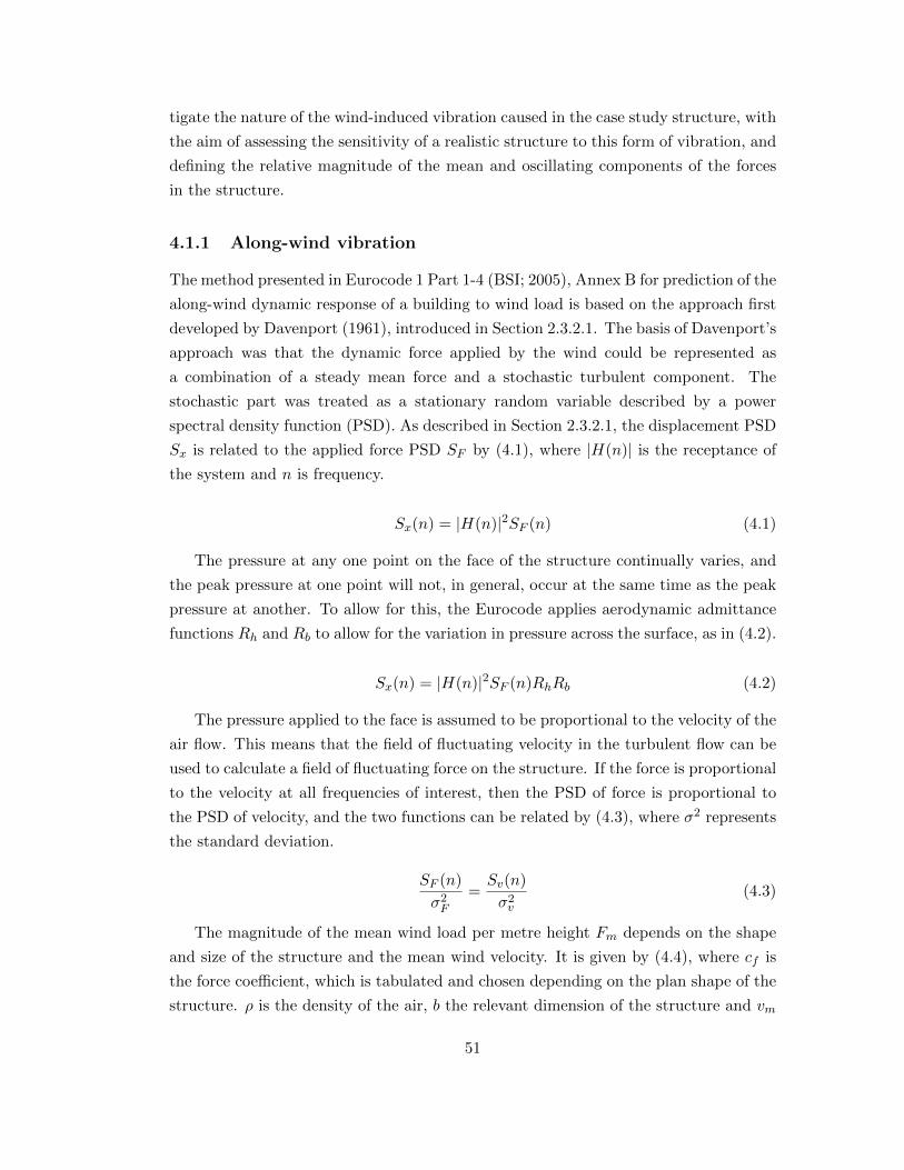
tigate the nature of the wind-induced vibration caused in the case study structure, with
the aim of assessing the sensitivity of a realistic structure to this form of vibration, and
defining the relative magnitude of the mean and oscillating components of the forces
in the structure.
4.1.1 Along-wind vibration
The method presented in Eurocode 1 Part 1-4 (BSI; 2005), Annex B for prediction of the
along-wind dynamic response of a building to wind load is based on the approach first
developed by Davenport (1961), introduced in Section 2.3.2.1. The basis of Davenport’s
approach was that the dynamic force applied by the wind could be represented as
a combination of a steady mean force and a stochastic turbulent component. The
stochastic part was treated as a stationary random variable described by a power
spectral density function (PSD). As described in Section 2.3.2.1, the displacement PSD
Sx is related to the applied force PSD SF by (4.1), where |H(n)| is the receptance of
the system and n is frequency.
Sx(n) = |H(n)|2SF (n) (4.1)
The pressure at any one point on the face of the structure continually varies, and
the peak pressure at one point will not, in general, occur at the same time as the peak
pressure at another. To allow for this, the Eurocode applies aerodynamic admittance
functions Rh and Rb to allow for the variation in pressure across the surface, as in (4.2).
Sx(n) = |H(n)|2SF (n)RhRb (4.2)
The pressure applied to the face is assumed to be proportional to the velocity of the
air flow. This means that the field of fluctuating velocity in the turbulent flow can be
used to calculate a field of fluctuating force on the structure. If the force is proportional
to the velocity at all frequencies of interest, then the PSD of force is proportional to
the PSD of velocity, and the two functions can be related by (4.3), where σ2 represents
the standard deviation.
SF (n)
σ2F=Sv(n)
σ2v(4.3)
The magnitude of the mean wind load per metre height Fm depends on the shape
and size of the structure and the mean wind velocity. It is given by (4.4), where cf is
the force coefficient, which is tabulated and chosen depending on the plan shape of the
structure. ρ is the density of the air, b the relevant dimension of the structure and vm
51

the mean wind velocity.
Fm = cfρbv2m (4.4)
The magnitude of the turbulent component of the force is represented by its root
mean square value σF , and the turbulence intensity lv is defined to relate σF and Fm,
by σF = l2vFm. This relationship can be combined with (4.3) and (4.4) to give (4.5).
SF (n) =(cfρbv
2ml
2v
)2 Sv(n)
σ2v(4.5)
(4.5) allows the PSD of the force applied to the structure to be calculated from the
PSD of the wind velocity. In the Eurocode, the PSD of the wind velocity is provided in
the form of a dimensionless PSD function which represents the distribution of frequency
components expected in a general wind load. This can then be scaled by the magnitude
of the turbulent component of the wind force, represented by σv, to be applied to a
specific site. The dimensionless PSD function SL(n) is defined by (4.6).
SL(n) =nSv(n)
σ2v(4.6)
Rearranging and substituting (4.6) allows (4.5) to be rewritten in terms of this
dimensionless PSD, as in (4.7).
SF (n) =(cfρbv
2ml
2v
)2 SL(n)
n(4.7)
(4.7) provides a way of calculating the properties of the dynamic force imposed on
a structure. In order to determine the response of the structure to this applied force,
(4.2) is used, so an expression is required for the receptance H(n) of the system. The
Eurocode uses the approach first proposed by Simiu and Scanlan (1986), of representing
a tall building structure as a slender, line-like vibrating object. The receptance function
for such an object for vibration at or near its first mode can be approximated by (4.8),
where fn is the natural frequency of the first mode, m is the equivalent uniform mass
per metre height and γ is the damping expressed as the proportion of critical damping.
i is the imaginary unit.
H(n) =1−
(nfn
)2− i(
2γ(nfn
))m (2πfn)2
((1−
(nfn
)2)2
+ 2γ(
2γ(nfn
))2) (4.8)
From (4.8), the magnitude of the receptance as a function of frequency can be
52

determined, and is shown in (4.9).
|H(n)| = 1
m (2πfn)2
√(1−
(nfn
)2)2
+
(2γ(nfn
)2) (4.9)
Using (4.2), (4.7) and (4.9), the along-wind vibration response of the structure can
be determined, and expressed as the PSD of displacement Sx. This function can then
be used to determine the PSD functions of velocity and acceleration Sx and Sx using
Sx = (2πn)2 Sx and Sx = (2πn)4 Sx. The PSD functions cannot be directly compared
with acceptability criteria, but most of the vibration limits described in Section 2.3.5
are expressed as the root mean square value of acceleration, which can be calculated
from the PSD of acceleration Sx according to (4.10).
σ2x =
∫ ∞0
S2xdn =
∫ ∞0|H(n)|2SF (n)RhRb (2πn)4 dn (4.10)
For small damping, the solution to the integral in (4.10) is dominated by the com-
ponent at resonance, and is approximately given by (4.11).
σ2x =πfn
4γm2SF (fn)RhRb (4.11)
This is the approximation used in the derivation of the Eurocode design method.
Adding a non-dimensional coefficient Kx, which accounts for the variation in wind force
through the height of the structure, a mode shape factor Φ(z), equal to 1 at the top of
the structure, to account for the variation of acceleration with height, and substituting
γ with δ = 2πγ, the logarithmic decrement of damping, gives (4.12), equivalent to
Equation B.11 in Eurocode 1 Part 1-4 (BSI; 2005).
σ2x =π2fn2δm2
SF (fn)RhRbKxΦ(z) (4.12)
The additional forces on the structure due to this vibration are then allowed for
using the coefficient cd, given by (4.13), where the resonance response factor R2 is
defined as in (4.14), B is a size effect factor which allows for non-correlation of pressures
over the face of the structure and kp is the ratio of the peak value of the turbulent
component of the wind velocity to the root mean square value which lv represents.
cd =1 + 2kplv
√B2 +R2
1 + 7lv√B2
(4.13)
R2 =π2
2δSLRhRb (4.14)
53

Figure 4-2: Strouhal number for buildings rectangular in plan, taken from Eurocode 1(BSI; 2005)
The Eurocode therefore provides a method for calculating the forces and accelera-
tions resulting from along-wind vibration due to turbulent wind load. The assumptions
inherent in the Eurocode design method are equally valid in their application to tim-
ber structures as they are to other structural materials, and it is considered that the
method can be used to investigate the effects of changing mass, frequency and damping
on the response of a case study structure.
In along-wind vibration, the forces in the structure have a mean value determined
by the mean wind velocity and the oscillation caused by turbulence moves around that
mean value. The magnitude of the oscillation in comparison to the magnitude of the
mean value will be investigated using the example structure in Section 4.1.3, and will
be important in determining the stiffness of the connections for that oscillation, given
the nonlinearity of the force-displacement behaviour of the connections.
4.1.2 Across-wind vibration
A method is also provided in Eurocode 1 Part 1-4 (BSI; 2005) for the assessment of the
across-wind vibration induced by vortex shedding, as described in Section 2.3.2.2. The
frequency of vortex shedding is calculated using the Strouhal number St. St = fL/V
where f is the frequency of vortex shedding, L is a characteristic dimension of the body,
and V is the velocity of the flow.
The Strouhal number for a particular structure depends on its shape in the plane
in which the vortices form. It is empirically derived, and for buildings rectangular in
plan it varies as shown in Figure 4-2.
For a particular structure, therefore, a critical velocity can be calculated at which
the frequency of vortex shedding is equal to the natural frequency of a structure, and
it is when this occurs that a severe vibration response can occur. Substituting fn,
the natural frequency of the structure in the relevant direction, for f and using b, the
54

Figure 4-3: Structure of the Barentshus building c©by Reiulf Ramstad Architects (Reid;2009)
across-wind breadth of the building, as the characteristic length, the relationship (4.15)
is obtained for the critical wind velocity vcrit,i.
vcrit,i =bfnSt
(4.15)
Across-wind vibration entails a full reversal of the forces in the structure with
each oscillation, and can be expected to be completely symmetrical about zero force.
Gap-formation in the connections in the lateral-load-resisting system can, therefore, be
expected to affect the stiffness of the connections and nonlinear connection behaviour
could lead to a variation of stiffness with amplitude of oscillation.
4.1.3 Tall timber building example
The structure which was chosen to illustrate the importance of this form of wind-
induced vibration is a conceptual tall timber building. It was based on the 20-storey
Barentsus building, proposed for the Norwegian town of Kirkenes. At the time of
writing, this project was on hold because of doubts about the demand for space in
a development of that size in that area. A preliminary design was carried out by the
engineers, Sweco, resulting in the geometry and member sizes described by Reid (2009).
The diagram in Figure 4-3, presented by Reid, illustrates the structural form.
55

Figure 4-4: Connection detail based on multiple-steel-plate dowel-type connection usedfor the Rena river bridge (Abrahamsen; 2008)
As well as investigating the global structural behaviour of this structure in response
to dynamic wind load, the influence of the connections on that behaviour was also of
interest. The information given by Reid (2009) did not address the connections, but
the multiple-steel-plate dowel-type connection used by Sweco in the Rena river bridge
(Abrahamsen; 2008) provided a realistic connection type for use in this example. That
connection was modified, and the form of connection modelled in this study is shown
in Figure 4-4.
The stiffness of the structure was assessed using a stiffness-matrix method, for a two-
dimensional elastic analysis of the frame structure, including a semi-rigid connection
stiffness, which allowed deformation of the connection in the two in-plane directions and
rotation. The structure was simplified into an 70m tall frame structure of twenty 3.5m-
high storeys, 24m × 24m in plan. Corner columns and bracing elements form trusses
in each face of the building and the floors are 180mm-thick cross-laminated timber
panels, which act as a diaphragm, distributing lateral loads to the vertical structure.
The lateral load was assumed to be resisted entirely by the trusses in each face of the
building, and so the lateral movement was assessed using a two-dimensional model of
one of these trusses loaded appropriately.
Two variations of the structure were modelled in order to assess the effect of con-
nection stiffness on its lateral deflection: truss connections fixed and semi-rigid truss
connections. The truss structure was broken up into elements 16m long or less, to
give approximately realistic member sizes for transportation, and the same connection
stiffness was applied between each element.
The flitch plates in the connection were modelled in each case as beam elements,
and at each connection between a timber member and the flitch plates, there was an
analysis node on the timber member and one on the flitch plates. In the undeformed
56

Table 4.1: Static deflections under mean wind load for the 20-storey glued-laminatedtimber structure
Truss connection Peak displacement Mean interstorey drift ratio(mm)
Fixed 119 height/670Semi-rigid 232 height/345
condition, these pairs of nodes had the same coordinates. In the case of the semi-rigid
connections, the connection between these nodes was assigned a rotational stiffness, and
a translational stiffness in each of the parallel- and perpendicular-to-grain directions. In
the fixed connections, the two nodes were constrained to translate and rotate together.
The connection stiffness was determined according to Eurocode 5 (BSI; 2009a),
for twenty-five 12mm diameter steel dowels arranged in a rectangular grid, and cross-
ing eight shear planes through the four steel plates slotted into each member. This
resulted in a rotational stiffness of 21025kNm/radian and a translational stiffness of
772963kN/m, and the same translational stiffness was applied both parallel and per-
pendicular to grain, since no effect of grain angle is allowed for in the Eurocode 5
method.
4.1.3.1 Static deflection under wind load
The force on the building due to the mean wind pressure was calculated according
to Eurocode 1 Part 1-4 (BSI; 2005), using a mean wind speed at sea level of 25m/s,
corrected for an altitude above sea level of 200m. This wind speed and altitude was
chosen to be sufficient to allow for all of the major cities in the United Kingdom,
and those conditions resulted in a total mean wind force on the building of 3662kN,
expected to occur, on average, once every 50 years. This force was distributed evenly
around the face of the building, and applied at each storey level.
The resulting deflections in each variation of the structure are shown in Table
4.1, including the interstorey drift ratio, calculated as δ/h, where δ is the horizontal
deflection and h the height. Figure 4-5 shows the model used for analysis and the
deformed shape.
The interstorey drift ratio is commonly used to assess the acceptability of static
deflections, in that it indicates the potential for deflections to cause damage to cladding
supported by the structure, and the potential for deflections to be visible to people
around the structure. The UK national annex to Eurocode 3 (BSI; 2008b) gives a
suggested acceptable interstorey drift ratio for steel structures of height/300. That
limit is considered to be a suitable guide for this example structure, since its primary
57
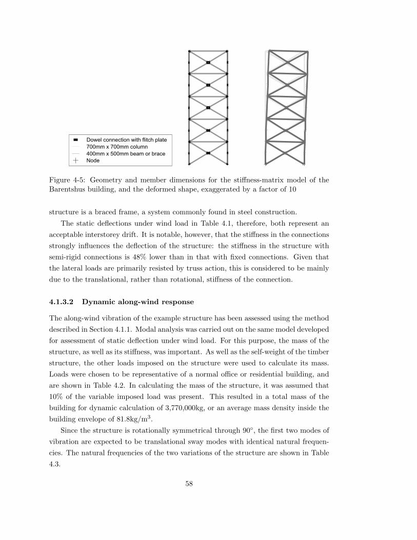
Dowel connection with flitch plate
700mm x 700mm column
400mm x 500mm beam or brace
Node
Figure 4-5: Geometry and member dimensions for the stiffness-matrix model of theBarentshus building, and the deformed shape, exaggerated by a factor of 10
structure is a braced frame, a system commonly found in steel construction.
The static deflections under wind load in Table 4.1, therefore, both represent an
acceptable interstorey drift. It is notable, however, that the stiffness in the connections
strongly influences the deflection of the structure: the stiffness in the structure with
semi-rigid connections is 48% lower than in that with fixed connections. Given that
the lateral loads are primarily resisted by truss action, this is considered to be mainly
due to the translational, rather than rotational, stiffness of the connection.
4.1.3.2 Dynamic along-wind response
The along-wind vibration of the example structure has been assessed using the method
described in Section 4.1.1. Modal analysis was carried out on the same model developed
for assessment of static deflection under wind load. For this purpose, the mass of the
structure, as well as its stiffness, was important. As well as the self-weight of the timber
structure, the other loads imposed on the structure were used to calculate its mass.
Loads were chosen to be representative of a normal office or residential building, and
are shown in Table 4.2. In calculating the mass of the structure, it was assumed that
10% of the variable imposed load was present. This resulted in a total mass of the
building for dynamic calculation of 3,770,000kg, or an average mass density inside the
building envelope of 81.8kg/m3.
Since the structure is rotationally symmetrical through 90◦, the first two modes of
vibration are expected to be translational sway modes with identical natural frequen-
cies. The natural frequencies of the two variations of the structure are shown in Table
4.3.
58

Table 4.2: Weights of cladding and finishes for calculation of the mass of the examplestructure
Element Imposed load Mass per unit area(kN/m2) (kg/m2)
Floor and ceiling services and finishes 1 9.81External cladding 1 9.81Variable load due to furniture and occupants 3 29.43
Table 4.3: Natural frequency of the first mode of vibration for the 20-storey glued-laminated timber structure
Truss connection 1st/2nd mode naturalfrequency(Hz)
Fixed 0.54Semi-rigid 0.39
Using the natural frequency, dimensions and mass of the structure, the design
method from Section 4.1.1 could be applied to determine the amplitude of acceleration
and the additional forces imposed on the structure by vibration. The method only
considers movement in the first mode of vibration.
There was some uncertainty in these calculated natural frequencies of the structure.
This was due to the fact that, as discussed in Section 2.2, the force-displacement
behaviour of dowel-type connections is not linear, so the secant stiffness they exhibit
depends on the mean and amplitude of the applied force. The stiffness calculated
according to Eurocode 5 (BSI; 2009a) is based on regression analysis of experimental
work by Ehlbeck and Larsen (1993). Details of the test results used for this regression
analysis were not published, but it is considered that they would have been carried out
according to the standard procedure at the time, EN 26891 (BSI; 1991), and so the
stiffness measured would have been the initial stiffness between the 10% and 40% load
levels. This initial stiffness was expected to be different from the secant stiffness under
the repeated cycles of load applied by wind-induced vibration, and it was that secant
stiffness which would determine the natural frequency.
Another important parameter in the vibration analysis which could not be accu-
rately determined was the modal damping. Eurocode 1 Part 1-4 (BSI; 2005) tabulates
damping estimates for various common structural forms, but gives no value for multi-
storey timber buildings. For timber bridges, the logarithmic decrement of structural
damping is suggested to be between 0.06 and 0.12, which equates to a range of equiv-
alent viscous damping ratio from 0.95% to 1.9%. Given that such damping estimates
59

0.1 10.01
0.1
1
Fundamental Natural Frequency (Hz)
Peak
Accele
ration (
m/s
)2
Offices
Residences
0.5
0.05
0.5
0.02
0.2 52
Figure 4-6: Suggested acceptable limits for lateral acceleration in wind-induced vibra-tion with a one-year return period, adapted from ISO 10137 (ISO; 2007)
are purely empirical, this is clearly an area which requires further research, and the de-
velopment of the energy dissipation which results in damping is considered throughout
the experimental and analytical work described in this thesis. For the analysis of this
example building, the damping estimates for timber bridges were used.
The uncertainty in natural frequency and damping was allowed for by performing a
sensitivity analysis on both. The natural frequency was varied between the values for
the semi-rigid and fixed connection conditions, and the damping was varied between
the lower and upper estimates given for timber bridges.
The acceptability of vibration was assessed against the ISO 10137 (ISO; 2007) stan-
dard, since it provides detailed acceptability criteria specifically for lateral vibration in
buildings. The proposed variation of acceptable acceleration with frequency for lateral
wind-induced movement from that standard is shown in Figure 4-6. That standard
states that, for a wind with a one-year return period, a peak acceleration of up to
55×10−3m/s2 at a frequency of 0.5Hz is suitable for residential buildings, and that up
to 80×10−3m/s2 is acceptable a general office building at the same frequency.
The parameters given for the wind load in Eurocode 1 Part 1-4 (BSI; 2005) represent
a 50-year return period wind event. In order to compare the results of the analysis with
the limits given in ISO 10137 (ISO; 2007), equation B.9 from the Eurocode was used
to calculate the one-year return period acceleration. With the symbols altered to use
the notation in this study, that equation is given in (4.16). σx,1 is the one-year return
period root mean square acceleration, and σx,50 is that for the 50-year return period.
Ng is the number of times the one-year value is expected to be exceeded in the 50-year
period, so was taken as 50. The one-year return period peak acceleration was then
60

0.07
0.09
0.11
0.45
0.5
0.2
0.25
0.3
0.35
Frequency (Hz)
Accele
ration (
m/s
)2
0.18
0.2
0.22
0.24
0.26
0.28
0.06
0.08
0.1
0.12
0.4
0.45
0.5
1
1.05
1.1
1.15
Frequency (Hz)
Dynam
ic F
acto
r c
d
1.02
1.03
1.04
1.05
1.06
1.07
1.08
1.09
1.1
1.11
δδ
Figure 4-7: Sensitivity analysis for vibration of example structure for frequency anddamping, δ - the left hand graph shows the peak acceleration, and the right hand graphthe magnification of the static mean force
calculated from the root mean square value using the peak factor given in Eurocode 1
Part 1-4 Annex B.
σ2x,1σ2x,50
= 0.007(logNg)2 − 0.174 logNg + 1 (4.16)
The variation of peak acceleration and peak force on the structure with natural fre-
quency and damping is shown in Figure 4-7. The additional force on the structure due
to vibration had a maximum value of approximately 12%, which can also be expressed
by saying the static force was increased by a ‘dynamic factor’ of 1.12.
Figure 4-7 shows that the acceptable limits of vibration for both residential and
office use were exceeded for the entire range of stiffness and damping considered in the
sensitivity study. The minimum peak acceleration was 0.168m/s2.
The results of the sensitivity study showed that for this example structure, which
achieved reasonable static deflections under wind load for serviceability, there was po-
tential for levels of wind-induced vibration which would affect its serviceability for
either office or residential use.
4.1.3.3 Dynamic across-wind response
The natural frequencies in Table 4.3 can be used to calculate the critical wind velocity,
the wind velocity at which vortices are shed at a frequency equal to one of its natural
frequencies, for the example structure using (4.15).
The building is 24m × 24m in plan, which gives a Strouhal number from Figure
4-2 of 0.12. The critical wind velocity for each variation of the connection conditions
is shown in Table 4.4. In each case, the critical wind velocity is higher than 78m/s,
which can be compared with a 1 in 50 year return-period wind speed of 25m/s. A severe
61

Table 4.4: Critical wind velocity for vortex shedding for the 20-storey glued-laminatedtimber structure
Truss connection 1st mode natural Critical windfrequency velocity(Hz) (m/s)
Fixed 0.54 108Semi-rigid 0.39 78
across-wind dynamic response therefore appears unlikely for this type of structure. The
low weight of the structure is an advantage in this context, since it leads to an increased
natural frequency, keeping the natural frequency above the expected frequency of vortex
shedding.
4.2 Footfall-induced vibration
The vibration induced by people walking, running, jumping or dancing on a structure,
individually or in unison, was discussed in Section 2.3.3. The nature of the oscillating
forces imposed by this form of vibration was studied using the case studies from the
literature summarized in Table 2.1.
It should be noted that there is some similarity in the distinction between vertical
and lateral vibrations due to footfall and the distinction between along-wind and across-
wind vibration due to wind load. Vertical vibration in floors or bridges produces an
oscillation of force around a mean force provided by the static loads on the structure,
while lateral footfall-induced vibration, on the other hand, can be expected to produce
an oscillating force around a zero mean force, as in the case of across-wind vibration.
For vertical vibration, the case studies in Table 2.1 show peak accelerations ranging
from 0.4m/s2 to 8.6m/s2. These accelerations give some indication of the variation of
force in the structure, since when the mass of the structure accelerates in the gravity
direction, the force in the structure is reduced. Once the mass has an acceleration
higher than the acceleration due to gravity, approximately 9.8m/s2, the force on it
reverses. A peak acceleration of 0.4m/s2, therefore, suggests that the lowest total force
on the mass would be 96% of the mean force on that mass, and 8.6m/s2 suggests a
lowest force of 12%. The accelerations at other parts of the structure would have been
lower, and so the oscillating forces correspondingly lower, but these values give an
indication of the magnitude of the oscillating force on the components in the structure,
and show that the force on the structure does not reverse under the vibrations in these
case studies.
62

Table 4.5: Examples of R-ratio calculation, compressive forces are positive
Example Highest Lowest R-ratioforce forceσmax (kN) σmin (kN) σmin/σmax
1 10 -10 -12 -10 -12 1.23 12 10 0.8333
Lateral vibration caused a serviceability failure of the Lardal timber and steel foot-
bridge and the dowel-type connections in that structure presented difficulties in accu-
rate prediction of its dynamic behaviour, as described in Section 2.3.3. In general, it is
considered reasonable to assume that no constant lateral load would be applied to the
structure to produce a mean value of the oscillating forces. Therefore, in the absence
of any prestress, the force on each element and connection in the structure resisting
the movement caused by lateral footfall-induced vibration would be expected to be
symmetrical about a zero mean.
4.3 Equivalent dynamic loads
The investigation of in-service vibration presented in this chapter was used to define
the dynamic loads applied in the experimental work in Chapter 5. Sections 4.1 and
4.2 show that in-service vibration can create oscillations of force in the structure which
range from a full reversal of load to a small oscillations around a non-zero mean.
To quantify this property of an oscillating load, a term is taken from the study of
fatigue: the R-ratio. The R-ratio relates the maximum and minimum values of the
oscillating load according to (4.17), where σmin is the numerical minimum stress and
σmax is the numerical maximum stress. In this study, the R-ratio is used to describe
the oscillating applied force, and a compressive applied force is represented as negative.
Table 4.5 has a few examples to clarify the calculation.
R =σminσmax
(4.17)
The highest dynamic force coefficient calculated for the example building in Section
4.1.3 was 1.12, which suggests an R-ratio for a component under compressive load of
1.27. The lowest dynamic force coefficient of 1.002 gives R=1.004. An R-ratio of 1.2
was chosen for the experimental work to be representative of the values calculated in
this sensitivity study. The fully-reversed oscillation due to across-wind vibration and
63

lateral footfall-induced vibration can be represented by an R-ratio of -1.
The problematic in-service vibration which has been described here is due to the
resonant response of a structure to a wide variety of dynamic applied forces. Regardless
of the nature of the applied force, if the response of the structure is resonant, then its
motion, and the forces induced, will be close to sinusoidal. In response to a stochas-
tic applied force such as turbulent wind load, the amplitude of that sinusoid will be
continuously varying. For the purpose of the experimental work in this study, it was
proposed to simplify the variable-amplitude near-sinusoidal vibration in real structures
to a pure sinusoid with constant amplitude.
4.4 Summary
In this chapter, the loads imposed on a structure due to in-service vibration have been
investigated. Representative ranges of the amplitude and frequency of these loads have
been presented by considering, by calculation and literature review, several forms of
wind- and footfall-induced vibration, and a simplified sinusoidal loading profile has
been proposed.
The next chapter will take this simplified loading and apply it in experimental work
to investigate the embedment of a connector into the timber that surrounds it under
dynamic load.
64

Chapter 5
Dynamic Embedment and
Connection Tests
In order to trace the processes responsible for connection stiffness and energy dissipa-
tion, and to develop models of those processes, a programme of dynamic testing was
developed which started with the basic part of a connection, and ended with a complete
frame with connections.
The basic part of the connection was taken to be the interaction between dowel and
timber as the circular section of the dowel is pressed into the hole cut in the timber.
This process is known as embedment. The experimental investigation of embedment
presented in this chapter formed the basis for two peer-reviewed journal papers. The
first addressed the elastic component of the embedment stiffness under cyclic load
(Reynolds et al.; 2013a), and the second the combination of elastic, viscoelastic and
plastic behaviour observed in the embedment tests (Reynolds et al.; 2013b).
In tests investigating the embedment behaviour in isolation, the dowel was held
rigidly straight, so that no deformation due to dowel bending occurred. Once the em-
bedment behaviour had been characterized, single-dowel connection specimens were
tested in which dowel bending contributed to the deformation, as in a complete con-
nection. The same analysis methods were applied to the results of both tests in order
to identify stiffness and energy dissipation, and the instrumentation was similar for
both, so they are presented together in this chapter.
5.1 Schedule of tests
Table 5.1 lists every physical test carried out as part of this study. The details of the
specimens and methods can be found in the relevant sections of this report. The tests
65

using servo loading machines are described in this chapter, and those using modal anal-
ysis and excitation by electrodynamic shaker or instrumented hammer are presented
in Chapter 7.
It can be seen that some specimens were tested only once, while others were used
for more than one test, using different load levels or forms of loading. This had conse-
quences for the statistical methods applied to each set of results, in that various tests
carried out on the same specimen could be considered as paired, while tests on different
specimens were independent.
5.2 Materials and Methods
5.2.1 Embedment test
Two species of timber were tested: Douglas fir and Norway spruce. The Douglas fir was
taken from solid timber grown in the south west of England, and the Norway spruce
from glulam graded GL28h according to BS EN 1194 (BSI; 1999), produced by Lillehe-
den in Denmark. The timber was stored after delivery in a controlled environment at
18-22◦C, and 60-65% relative humidity. The Norway spruce had been kiln dried before
being glue-laminated, and so was assumed to be near equilibrium moisture content on
delivery. This assumption was justified by the moisture content measured after testing,
given in Section 5.3.1. A piece of Douglas fir was tested for moisture content according
to the oven-dry method given by EN 13183 (BSI; 2002b) on delivery, and found to have
a moisture content higher than 25%. The timber was therefore stacked with spaces to
allow air drying in the controlled environment, and the change in moisture content
estimated by monitoring the weight of a 2m-long piece with cross section 60mm ×300mm. The change in moisture content from the delivery date to the start of testing
is shown in Figure 5-1. The moisture content estimated this way, at between 14 and
15%, corresponds closely to the moisture content measured by the oven dry method
and given in Section 5.3.1.
In the Douglas fir, a 20mm diameter steel dowel was placed in a half-hole in the
timber drilled using a 20mm auger drill bit, and in the Norway spruce, a 12mm diameter
dowel in a hole drilled using a 12mm auger drill bit. Embedment specimens were also
made for screws in Norway spruce, using screws provided by Spax with 7.5mm internal
diameter, 12mm external diameter and 6mm pitch. 6mm holes were predrilled for the
screws, which were installed between two pieces of timber held together in a vice, as
recommended in ASTM D5764 (ASTM; 1997), so that the two pieces could then be
separated to leave the screw installed in a half-hole in the timber, as shown in Figure
5-2. In each case, both parallel- and perpendicular-to-grain specimens were tested, and
66

Table 5.1: Schedule of physical tests
TestsGrain including
Test Materials direction Specimens repetitions
Load applied using a servo loading machine
Material Douglas fir Para. 26 26character- Perp. 26 26ization
Norway spruce Para. 18 18Perp. 18 18
Cyclic Douglas fir and 20mm plain Para. 19 19embedment steel dowel Perp. 18 18
Norway spruce and 12mm Para. 4 16plain steel dowel Perp. 3 12
Norway spruce and 12mm Para. 3 12steel screw Perp. 3 12
Single-dowel Norway spruce glulam and Para. 3 12connection 12mm plain steel dowel Perp. 3 12
Excitation by an electrodynamic shaker or instrumented hammer
Moment Norway spruce glulam, steel - 4 8connection connecting plates and six
12mm plain steel dowels
Norway spruce glulam, steel - 2 9connecting plates and two12mm plain steel dowels
Portal frame Norway spruce glulam, steel - 2 14connecting plates and 12mmplain steel dowels
67

0.00%
5.00%
10.00%
15.00%
20.00%
25.00%
30.00%
14/09 24/10 03/12 12/01 21/02
Day/Month
Estim
ate
d M
ois
ture
Conte
nt
Figure 5-1: Variation in moisture content of Douglas fir stored at 18-22◦C, and 60-65%relative humidity
were chosen to be free from knots or splits. The perpendicular-to-grain direction varied
between radial and tangential, according to how the plank or laminate had been cut
from the log, as would be the case in a real structure.
It was noted that this variation in grain orientation would introduce scatter into the
perpendicular-to-grain test results. One approach to reducing this scatter would have
been to divide the specimens into sets with different radial-tangential grain orientation,
or to classify them by an angle in the radial-tangential plane. Given that the relevant
objective of this study was to characterize the embedment behaviour for prediction
of the behaviour of complete connections and frames, it was considered that such a
study would not make the appropriate contribution. Since the orientation of loading
in the radial-tangential plane is not generally known in structural design, and since
in glued-laminated timber, a connector would embed into laminates with a variety of
such grain angles, it was considered more relevant to measure the perpendicular-to-
grain behaviour with a realistic variation of grain angles in the radial-tangential plane.
The full set of embedment test specimens is shown in Table 5.2. Where four rep-
etitions were used rather than three, this was due to an extra test being carried out
to replace tests in which an error in measurement or data logging was thought to have
occurred, but it was subsequently found that all the results could be used.
A separate Douglas fir specimen was used for every variation of peak force and
R-ratio, which resulted in a total of 37 specimens. For the Norway spruce tests, each
specimen was tested at the full range of loads and R-ratios, so only 6 specimens were
used.
68

Table 5.2: Cyclic embedment tests
Species Grain orientation Peak compressive R-ratio Number offorce repetitions
Douglas fir Parallel 20% 1.2 3and 20mm dowel 10 4
40% 1.2 310 3
80% 1.2 310 3
Perpendicular 20% 1.2 310 3
40% 1.2 310 3
80% 1.2 310 3
Norway spruce Parallel 20% 1.2 4and 12mm dowel 10 4
40% 1.2 410 4
Perpendicular 20% 1.2 310 3
40% 1.2 310 3
Norway spruce Parallel 20% 1.2 3and screw 10 3
40% 1.2 310 3
Perpendicular 20% 1.2 310 3
40% 1.2 310 3
69

Figure 5-2: Parallel-to-grain screw embedment specimen
As described in Section 2.2.1, embedment tests have been widely used to identify
both static and dynamic characteristics of the interaction between dowel and timber.
This study required experimental evidence of the stiffness and energy dissipation in
embedment under dynamic loads well below the yield load. This meant that the dis-
placement and energy dissipation to be measured were smaller than in the tests reviewed
in Section 2.2.1, where gross plastic behaviour generally occurred in the timber.
In defining a suitable test method to measure the small displacements expected
in the timber, the magnitude of the displacements to be measured had to be com-
pared both to the resolution of the measurement equipment, and the magnitude of the
deflections occurring in the test equipment rather than the specimen.
5.2.1.1 Geometry of specimen and loading apparatus
As has been discussed in Section 2.2.2, there are two widely-used methods for deter-
mining embedment properties of timber: the ASTM method (ASTM; 1997), which uses
a timber block with a half-hole in its surface, and the EN method (BSI; 2007), which
uses a timber block with a full hole through it. The EN method has the clear advantage
that it matches the situation in a real connection, and, on that basis, the first pilot
tests carried out for this study used the geometry according to the EN method. The
test setup is shown in Figure 5-3.
The EN test method requires the displacement readings to be calibrated to account
for dowel bending based on the displacement where the timber specimen is replaced by
a ‘tight-fitting steel piece’. The geometry of the steel piece is not specified.
70

Steel loading piececlamped into loadingmachine
Specimen supportedon bed of loadingmachine
Figure 5-3: EN383 embedment test method used in pilot tests (BSI; 2007)
It is assumed that the calibration method is based on the assumption that the de-
formation of a steel piece is insignificant in comparison to the deformation of the timber
specimen under the same load. There are some inaccuracies inherent in this calibra-
tion method, which are prominent particularly when applied to the high embedment
stiffness associated with small-amplitude cyclic loading.
As the dowel embeds into the timber during an embedment test, the dowel will
assume a deformed shape which depends on the stiffness of the dowel and the resistance
of the timber. In contrast, when bearing on the relatively stiff foundation formed
by the steel piece, the deformed shape of the dowel will be determined by the much
higher stiffness of the steel. A steel piece as wide as the loading fork would prevent
deformation of the dowel, and a thin steel piece would allow dowel deformation, but in
a very different deformed shape to that caused by the timber specimen. Calibration
with a steel piece cannot, therefore, be used to calculate the contribution of dowel
deformation to the measured deflection in the test.
In this study a test with a steel piece was used to give an indication of the order
of magnitude of the deflection due to deformation in the dowel. The same dynamic
load was applied to the steel piece as to the timber. The timber piece was 60mm thick,
and a steel piece 50mm thick was used, so as to allow some bending deformation of
the dowel. The resulting force-displacement diagrams for the timber specimen and
the steel piece are shown in Figure 5-4. While the test with the steel piece does not
replicate the deformed shape of the dowel in the EN embedment test, the results in
Figure 5-4 suggest that the contribution of the deformation of the loading apparatus
71

1.44 1.45 1.46 1.47 1.48
16
16.5
17
17.5
18
18.5
19
Displacement (mm)
Forc
e (
kN
)
0.27 0.28 0.29 0.3
16
16.5
17
17.5
18
18.5
19
Displacement (mm)
Forc
e (
kN
)
Figure 5-4: Comparison of force-displacement diagrams for a single cycle of appliedforce at 1Hz for the EN embedment test (left), and a test in which the dowel bears ona steel piece (right)
and dowel to both the secant stiffness and energy dissipation is of a similar magnitude
to the stiffness and energy dissipation in the timber itself.
The displacement in the test with the steel specimen is approximately the same
as in the test with the timber specimen under the same load, which suggests a sig-
nificant contribution of dowel deformation to the measured displacement. The energy
dissipation, represented by the area inside the force-displacement loop, is similar in the
two tests, which suggests a large contribution from dissipative processes in the loading
apparatus.
The validity of this part of the study relies on accurate measurement of stiffness and
energy dissipation caused solely by the timber and the interaction between dowel and
timber at their interface. The test method was therefore altered to eliminate, where
possible, the flexibility and energy dissipation in the loading apparatus.
By using the ASTM embedment test method, shown in Figure 5-5, the load could
be applied to the dowel by direct contact with the loading head of the test machine,
providing the minimum load path through the loading apparatus, and minimizing de-
formation and energy dissipation from that source. By applying the load this way, the
dowel was held rigidly straight by the loading head, ensuring no dowel deformation and
an evenly applied displacement over the width of the timber specimen. This method
was therefore considered preferable to the EN method for the purpose of these cyclic
embedment tests, and was used for all those embedment tests described in this section.
The drawback of the ASTM method is that the specimen does not have the same
geometry as the timber subject to embedment by a dowel in a connection, since the
timber on the unloaded face of the hole is not present. The effect of this difference is
discussed in detail in Section 2.2.2, with reference to the study by Santos et al. (2010).
The data from the numerical model presented in that paper suggested a variation in
stiffness of approximately 10% resulting from the difference in test method. For the
72

Connector
Applied Force
Timber Piece
Displacement measuredbetween loading headand test bed
Height
ThicknessWidth
Figure 5-5: Test setup and specimen dimensions for the ASTM embedment test method(ASTM; 1997)
purpose of this study, it is considered that the reliability of measurements of foundation
modulus and energy dissipation given by the ASTM method outweigh the benefit of
the more accurate geometry in the EN method, in which there would be significant
contributions to both measurements by the loading apparatus which could not be
readily measured.
The specimen dimensions were chosen to comply both with the requirements of the
ASTM method, which specifies minimum dimensions, and, for comparison, with those
of the EN method. The specimen dimensions are shown in Table 5.3.
Table 5.3: Specimen dimensions for embedment tests
Dowel/Screw Grain Width (mm) Height ThicknessDiameter (mm) Orientation (mm) (mm)
Norway spruce12 Parallel 72 84 40
Perpendicular 168 50 40Douglas fir20 Parallel 120 140 60
Perpendicular 280 80 60
5.2.1.2 Measurement of force and displacement
The load applied to the specimen was measured by the load cell integrated with the
servo-hydraulic loading machine. The resolution of this measurement was a key consid-
eration in the choice of loading machine for these experiments. In order to identify the
noise in readings taken from them, force readings were recorded from the load cells in
each of three potential loading machines for the tests, with no load applied. The out-
put force readings could then be inspected, and the noise represented by the standard
deviation of the readings, and the resolution by the minimum step between readings.
The data for each machine was logged on the same Vishay System 6000 data logger, so
73

Table 5.4: Noise measurements for servo-hydraulic loading machines
Loading machine Standard deviation of noise Resolution(kN) (kN)
Denison Mayes 20t 0.0002819 0.000343Dartec 10t 0.0024394 0.003052Instron 10t 0.0063568 <0.00007
the contribution of the data logger to both resolution and noise was the same in each
case.
The machines tested were a 20-tonne capacity Denison Mayes, a 10-tonne capacity
Dartec and a 10-tonne capacity Instron. The measurement range of the Denison Mayes
machine could be adjusted, and the lowest available range of ±20kN was used to provide
the minimum amplitude of noise in the force measurement. The resulting standard
deviation of force for each machine is shown in Table 5.4. The results show that,
although the resolution of the Instron was highest, it showed far more noise under zero
load than the Denison Mayes. The Instron and Denison Mayes machines were located in
different laboratories, and so it is possible that a difference in electromagnetic activity
in each location caused this difference in noise. Because of its lower noise, the Denison
Mayes machine was chosen for the tests in this study.
Displacement was measured in the pilot tests using strain-gauge-based displacement
transducers in which contact between the transducer and the part to be measured is
maintained by the force generated by a spring. The clamp-and-stand support for the
transducer, therefore, resisted the reaction from this spring force. Where the displace-
ments to be measured were of the order of tenths of millimetres, the deformation of the
clamp-and-stand, assembled with reasonable tightness, could be assumed to be small
in comparison to the displacements to be measured.
Given the small deformations to be measured in this study, of the order of microns,
it could not be assumed that the support for the transducer would not displace signifi-
cantly in comparison with the displacements to be measured as a result of the reaction
from the spring force. This deformation, and its effect on the measured displacement,
were thought to be partly responsible for the very high apparent energy dissipation,
shown by a large hysteretic loop, found in some pilot tests.
Further pilot tests were carried out with stiffer supports for the displacement trans-
ducers, which yielded a lower measured energy dissipation. Whether the deformation
of the support was significant compared with the deformation to be measured, how-
ever, remained uncertain. Given this fact, and the need for improved resolution of the
displacement measurements for calculation of energy dissipation, it was considered ap-
74

Rod screwed tomagnet
LVDT body unconnectedto rod
Moving head ofloading machine
Fixed base ofloading machine
Figure 5-6: Linear variable differential transformer with the rod connected to the load-ing head by a magnet
propriate to obtain another sensor for these measurements. A non-contact sensor was
used to ensure that no force was applied to the support at all, removing the uncertainty
in its displacement.
The non-contact sensor which was used was a Micro-Epsilon ±1mm linear variable
differential transformer (LVDT), which measures displacement by the differential volt-
age created by a metallic rod moving through an inductive coil. In the LVDT model
chosen, the rod was not connected to the body of the sensor, and so was connected only
to the part of the test apparatus to be measured, the head of the loading machine, by a
permanent magnet, as shown in Figure 5-6. The rod therefore moved freely relative to
the body of the sensor, ensuring no transfer of force between the two, and no variable
load to be resisted by the support for the sensor.
5.2.1.3 Definition of loading profiles
Amplitude of cyclic component The types of load which were of interest in this
study were discussed in Chapter 4, and the magnitude and form of oscillating load to
be applied in this experimental work in Section 4.3. The result was that a sinusoidal
variation of force should be applied, the mean and amplitude of which was defined by
the R-ratio. R-ratios of 1.2 and -1 were shown to be representative of different forms
of in-service vibration.
In the chosen embedment test method, however, only compressive loads could be
applied to the half-hole specimen. The R-ratio of 1.2 could therefore be tested, but the
R-ratio of -1 was not possible. Instead, an R-ratio of 10 was used, meaning that the
75

compressive applied load cycled between its maximum value and 10% of that maximum,
to investigate the effect of near-removal of the load on that face of the hole. It was
not considered safe to use a load of less than 10% of the maximum, in case a slight
overshoot led to load reversal and excessive movement of the loading head. It should
be noted that, as a result of an overshoot of the lower value of compressive load, the
minimum load was often less than 10% of the maximum, so the R-ratio of 10 should
be considered a nominal value corresponding to near-removal of the load.
The frequency of the oscillating load was 1Hz in the majority of tests, chosen to be
within the range of vertical and lateral structural vibration. Vertical footfall-induced
vibration generally occurs at frequencies higher than 1Hz, and the lateral mode natural
frequency of tall buildings can be lower, but 1Hz was considered to be a reasonable
frequency to investigate the general principles of vibration behaviour in this range.
Magnitude of peak load It was intended that the specimens be tested at loads
representative of those they would experience in normal service conditions, such as
a turbulent wind load which is expected to occur once per year. To illustrate the
relationship between the expected capacity of a structural element and the load on
that element expected to occur annually, the following example is given, for a timber
connection under wind load, designed according to the Eurocode method. It has been
assumed that the element is designed to work to its full efficiency, so that the ultimate
limit state load is equal to the ultimate limit state resistance. The relationship is
summarized in Figure 5-7.
First, the load carrying capacity, or resistance, was considered: the relationship
between the expected resistance of a connection and the design resistance is defined
by the statistical properties and partial factors applied by design codes. In design
according to Eurocode 5 (BSI; 2009a), either tests or an empirical calculation based
on density are used to determine a characteristic value of the embedment strength of
the timber, which is exceeded by 95% of specimens. The expected value, the mean
embedment strength, is higher than this characteristic value. In the tests by Santos
et al. (2010), a standard deviation of 13% for the parallel-to-grain specimens and 18%
for perpendicular to grain was recorded. Assuming a normal distribution, the 95th
percentile will be approximately 1.64 standard deviations below the mean. Taking the
average of the two grain orientations, the 95th percentile would be approximately 75%
of the mean value. The design value of a resistance Rd is then obtained from 5.1, in
which Rk is the characteristic value of the resistance. The material partial factor γM
is taken as 1.3 for solid timber, and kmod as 0.9 for a short-term action.
76
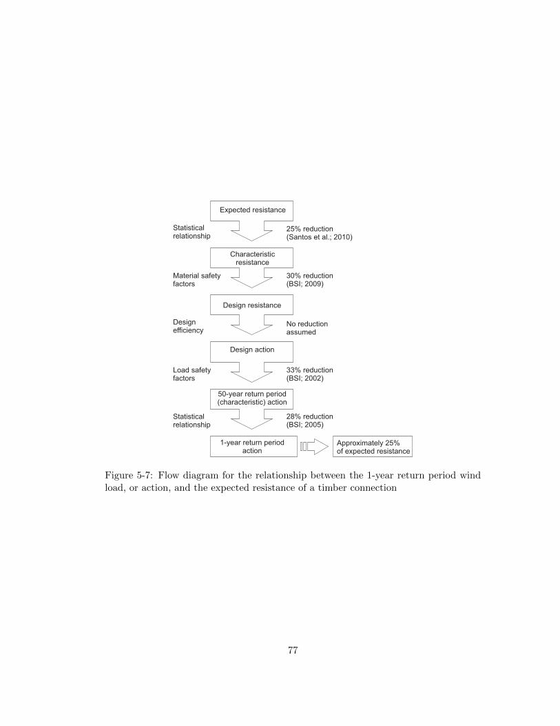
Expected resistance
25% reduction(Santos et al.; 2010)
Characteristicresistance
30% reduction(BSI; 2009)
Design resistance
1-year return periodaction
50-year return period(characteristic) action
Design action
28% reduction(BSI; 2005)
33% reduction(BSI; 2002)
Statisticalrelationship
Material safetyfactors
Designefficiency
Load safetyfactors
Statisticalrelationship
Approximately 25%of expected resistance
No reductionassumed
Figure 5-7: Flow diagram for the relationship between the 1-year return period windload, or action, and the expected resistance of a timber connection
77

Rd =RkkmodγM
(5.1)
The design value of the resistance is therefore 70% of the characteristic value, and
approximately 50% of the mean value.
Next, the applied loads were considered: Eurocode 1 Part 1-4 (BSI; 2005) uses
characteristic values of loads that are deemed to be exceeded once in 50 years. The
same code also gives an equation to determine the load for different return periods,
which is given as (4.16). Using this equation, the 1-year return period load is 72%
of the characteristic load. The design value of an applied load is then obtained using
factors in Eurocode 0 (BSI; 2002a), which are recommended as 1.35 for a permanent
action, and 1.5 for a variable action.
As a result of these statistical relationships and safety factors, for this scenario, the
1-year return period load is 25% of the expected value of the capacity of the connection,
or 34% of the characteristic capacity.
For the test programme, peak loads of 20% and 40% of the predicted characteristic
capacity were applied, in order to cover the range of loads imposed on a connection in
service. The characteristic capacity was predicted using the method given in Eurocode
5 (BSI; 2009a), which determines the embedment strength by an empirical equation
based on density at 12% moisture content. The density of each species of timber
was therefore measured and adjusted for the measured moisture content. For the
Douglas fir, since the specimens were not taken from graded structural timber, two
static embedment tests were carried out according to BS EN 383 (BSI; 2007) in each
grain direction to check that the predicted embedment strength was reasonable.
Number of cycles The duration of loading was chosen to ensure that any transient
effects could be observed and that a single value of either stiffness or energy dissipation
could be measured which was representative of the long-term steady-state behaviour.
The load was applied for 1000 cycles, which, during the pilot tests, proved sufficient for
the stiffness and energy dissipation to reach a representative steady state. There was
some evidence of a continued variation in stiffness and energy dissipation up to the end
of the 1000-cycle test, which was more prominent in some tests than others, but it was
considered that 1000 cycles represented a reasonable compromise between the need to
achieve a steady-state response and the available time for testing.
78

5.2.2 Single-dowel connection test
The single-dowel connection test was intended to investigate the processes which con-
tribute to stiffness and energy dissipation once the dowel is permitted to deform as in
a complete connection. As discussed in Chapter 3, the connection tests and analysis in
this study were restricted to one type of connection, in which the dowel transmits force
from the timber to a steel plate in a central slot. Tensile and compressive loads were
applied to each specimen to investigate the effect of the different stress distributions
in the timber on stiffness and energy dissipation. In order to keep energy dissipation
from sources other than the connection to a minimum, it was decided to avoid the
need to anchor the specimen by making it symmetrical, with an identical connection
at each end. Only the deformation of the loading head was measured, so the measured
deformation represented the sum of the deformations in the two identical connections.
The test specimens were cut from 185mm by 200mm glued laminated timber beams
made of Norway spruce, graded GL28h according to BS EN 1194 (BSI; 1999), and
supplied by Lilleheden. The beams were made up of five 40mm laminates, and as a
result, both the parallel-to-grain and perpendicular-to-grain specimens contained glue
lines. Specimens were rejected if they contained a substantial visible defect in the
surface of the timber within 25mm of the holes for the connectors. Otherwise, the
specimens were used as-delivered, incorporating the defects elsewhere in the timber.
BS EN 383 (BSI; 2007) gives recommended dimensions for a symmetrical tensile
test specimen parallel-to-grain, and so these dimensions were used to aid comparisons
with work by other researchers. No guidance is given in EN 383 (BSI; 2007) for tensile
tests perpendicular-to-grain, so the specimen dimensions were determined to match the
compressive tests in that standard. The specimens are shown schematically in Figure
5-8, and a photograph of the tests in each grain orientation is in Figure 5-9. The cyclic
loading applied to the single-dowel connection test specimens was the same as for the
embedment tests, with the addition of a fully-reversed test with an R-ratio of -1.
The specimens for perpendicular-to-grain loading did not have a sufficiently large
cross-section to ensure failure by dowel yield and embedment under tensile loading.
The failure mode under tensile loading would instead have been expected to be by
tensile failure of the timber between the dowels. The cross-section was, however, large
enough to ensure that loads of 20% and 40% of the yield load of the connection could
be applied without tensile failure of the timber. This meant that cyclic loading tests
could be carried out in both tension and compression on the perpendicular-to-grain
specimens up to 40% of the yield load of the connection, but static load tests to failure
were only carried out in compression, to avoid brittle failure by splitting.
The single-dowel connection tests were carried out in displacement control, since it
79
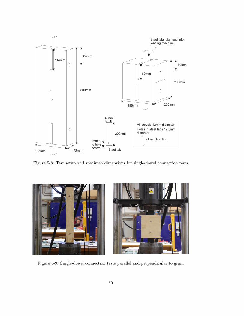
185mm 72mm
800mm
185mm 200mm
200mm
Steel tabs clamped intoloading machine
Grain direction
50mm
84mm
200mm
All dowels 12mm diameter
114mm
80mm
40mm
26mmto holecentre
Steel tab
Holes in steel tabs 12.5mmdiameter
Figure 5-8: Test setup and specimen dimensions for single-dowel connection tests
Figure 5-9: Single-dowel connection tests parallel and perpendicular to grain
80

was found in pilot tests that in load control, the servo-hydraulic loading machine did
not reliably achieve the target peak and trough forces, occasionally becoming unstable.
For the small-amplitude oscillating loads, particularly at 20% of the predicted yield
force and R=1.2, a noticeable oscillation at a frequency higher than the 1Hz test
frequency appeared to be superimposed on the sinusoidal oscillation of the loading
head. This was recognized to be a movement of the loading head, rather than a
measurement noise, since it was measured by the LVDT and produced a corresponding
force in the load cell. It is thought that this small-amplitude movement may be the
‘dither’ in the servo-hydraulic system: a continuous movement imposed to avoid static
friction in the components of the loading machine.
The movement resulted in brief reversals in the force-displacement plot, and so
small loops within the overall hysteretic loop. While it was not considered that this
behaviour significantly affected the shape of the overall force-displacement response, it
was noted that each loop would cause additional energy dissipation not representative
of the energy dissipation of the specimen under sinusoidal load. In order to remove
the effect of these loops, the energy dissipation was calculated based on the area of a
smoothed envelope curve around the measured force-displacement response.
The smoothing was achieved by applying a low-pass filter to both the force and
displacement measurements. A 1-pole digital filter was applied using the MATLAB
function filter. Figure 5-10 shows the effect of applying the filter with cutoff frequen-
cies of 3.2Hz and 6.4Hz. It can be seen that, as well as removing higher-frequency
components of the signal, the filter induces a phase lag. The cutoff frequency of 6.4Hz
was chosen to achieve adequate smoothing of the signal without excessive phase lag.
5.2.3 Analysis
The aim of this study was to identify the contribution of connections to natural fre-
quency and damping in structures. The natural frequency is determined by the combi-
nation of the stiffness of each component of the structure, and the damping by the com-
bination of their energy dissipation. For both the embedment tests and the single-dowel
connection tests, the stiffness and energy dissipation were therefore to be determined.
Since the force-displacement response was not perfectly linear-elastic, a range of
stiffnesses was exhibited under loading and unloading. The secant stiffness was chosen
as the representative stiffness for each cycle of applied load, and was measured for
each specimen and each cycle. The secant stiffness was taken as the average gradient
on the force-displacement plot between the two extreme values of displacement. For
behaviour under cyclic load which was close to linear, as in the left-hand graph in
Figure 5-11, the secant stiffness closely followed the lines of loading and unloading
81

Dis
pla
cem
ent (m
m)
5.15 5.16 5.17 5.182
2.5
3
Displacement (mm)
Original measured data
5.15 5.16 5.17 5.18
Displacement (mm)
175 176
1.5
2
2.5
3
3.5
Time (s)
Applie
d F
orc
e (
kN
)
175 176
Time (s)
Applie
d F
orc
e (
kN
)
Time (s)
175 176
Time (s)
175 1765.1
5.15
5.2
Filtered data
6.4Hz Cutoff Frequency 3.2Hz Cutoff Frequency
175.5 176.5174.5 175.5 176.5174.5
175.5 176.5174.5175.5 176.5174.5
Figure 5-10: Filtering force and displacement measurements: the first row of figuresshows the effect of applying a low-pass digital filter to the force measurements, thesecond row shows the effect on the displacement measurements, and the third theforce-displacement loop for the indicated cycle
82

0.16 0.2 0.240
2
4
6
8
10
12
14
Displacement (mm)
Forc
e (
kN
)
0.236 0.24 0.244 0.248
11.5
12
12.5
13
13.5
14
Displacement (mm)
Forc
e (
kN
)
Single cycleSecant
Single cycleSecant
Figure 5-11: Secant stiffness for one-sided vibration with different amplitudes
closely. For non-linear behaviour, as in the right-hand graph in Figure 5-11, the secant
line deviated from the lines of loading and unloading. Nonetheless, the secant stiffness
was considered to be the appropriate parameter by which to represent the stiffness of
each cycle. Whether this linear parameter is a sufficiently accurate representation of
the non-linear behaviour is investigated in Chapter 7.
The energy dissipation in each cycle is given by the integral of the work done by
the applied force around that cycle, which is equal to the area inside the hysteretic
loop on the force-displacement diagram. If the force is expressed in Newtons, and the
displacement in metres, then the work done calculated is in Joules. For structural
engineering purposes, it is useful, and common, to express energy dissipation in a
component as the damping it would generate if it was supporting a vibrating mass. In
this study, it is expressed in terms of the viscous damping ratio γ. The relationship
between γ and the energy dissipated is derived in various text books, such as by Thorby
(2008), but the force-displacement response in these tests differs from the form generally
derived, in that the oscillating load is not symmetrical around zero, and the locally
linear line of secant stiffness does not necessarily pass through the origin. It is therefore
considered useful to derive the relationship for this particular case.
If the stiffness supporting the mass is k, the viscous damping coefficient c and the
mass m, then the equation of motion of the system would be as given in (5.2), where x
is the displacement of the dowel or connection, and the overdot denotes differentiation
with respect to time, t. To allow for the possibility that the force-displacement rela-
tionship is only locally linear, the constant A is added, so that the displacement for
zero elastic force is not necessarily zero.
mx+ cx+ k(x+A) = F (5.2)
The natural frequency of the system is usually assessed by looking at the solution
83

to this equation under zero applied force. In this case, the solution for zero applied
force is not of interest, but the solution for oscillation around a non-zero mean force
is. In (5.2), for oscillation around a mean force F = kA, the equation simplifies to the
normal equation of motion for a single-degree-of-freedom system. The system therefore
has circular natural frequency ωn, unaffected by A, where ωn =√k/m.
In the experimental work in this study, the low mass of the specimen and dowel
compared with its stiffness means that the inertial force mx is small compared with
the forces due to stiffness and damping. The equation of motion can, therefore, be
simplified to cx+ k(x+A) = F .
The energy dissipated in each cycle E, equal to the area inside the hysteretic loop
on the force-displacement diagram is given by (5.3), where τ is an arbitrary start time
and T is the period of oscillation.
E =
∮Fdx =
∮F
dx
dtdt =
∫ τ+T
τFxdt (5.3)
Suppose the test is being carried out in displacement control, so that x = X sin(ωt)+
B and x = ωX cos(ωt), where X is the half-amplitude of the applied displacement, ω
is its circular frequency and B is an arbitrary offset of the displacement from zero.
The applied force can then be expressed as F = k(X sin(ωt) + A+B) + cωX cos(ωt),
T = 2π/ω and the energy dissipated is given by (5.4).
E =
∫ τ+2π/ω
τ(k(X sin(ωt) +A+B) + cωX cos(ωt))ωX cos(ωt)dt (5.4)
(5.4) can be expanded to give (5.5).
E =
∫ τ+2π/ω
τkωX2 sin(ωt) cos(ωt) + k(A+B)ωX cos(ωt) + cω2X2 cos2(ωt)dt (5.5)
The integrals of both cos(ωt) and sin(ωt) cos(ωt) over a complete period are zero,
so (5.5) can be simplified to (5.6).
E = cω2X2
∫ τ+2π/ω
τcos2(ωt)dt = πcX2ω (5.6)
The viscous damping ratio γ is given by γ = (cωn)/(2k). Substituting for c and
rearranging gives (5.7).
γ =E
2πkX2 ωωn
(5.7)
84

Hence the energy dissipated in a specimen with viscous damping, E, calculated
from tests, is related to the viscous damping ratio in an oscillating system with the
same stiffness and viscous damping coefficient, γ by (5.7). It can be seen that the offsets
in elastic force kA and displacement B have no effect on the calculation, as long as
the behaviour is linear between the two extreme values of displacement, so that it can
be described by (5.2). The ω/ωn term in (5.7) arises because, in the viscous damping
model, the energy dissipated varies with frequency, so it allows for the general case in
which the test frequency ω is not the same as the resonant frequency ωn.
The viscous damping model does not necessarily apply to dowel-type connections.
An alternative damping model, the hysteretic damping model, states that the damping
force is proportional to the amplitude of displacement, but in phase with the velocity.
This means that, in the hysteretic damping model, the damping force is independent
of the magnitude of the velocity, and so independent of the frequency. Thorby (2008)
presented the same relationship as (5.7) for the hysteretic damping model. For the same
applied displacement and velocity, the force is then given by (5.8), and the integral in
(5.3) yields (5.9). Again, applying the offsets A and B, as in (5.4), has no effect. The
hysteretic damping coefficient for a specimen can, therefore, be calculated from (5.10).
F = kX sin(ωt) + gX cos(ωt) (5.8)
E = πkX2g (5.9)
g =E
πkX2(5.10)
Whether the viscous or hysteretic damping model should be applied to dowel-type
timber connections depends on the measured variation of damping with frequency,
discussed in Sections 5.3.2 and 5.3.3.
5.2.4 Statistical hypothesis testing
The influence of the magnitude of the peak load on the steady-state secant stiffness
measured in the tests was investigated using Student’s t-test, attributed to William
Sealy Gosset (Student; 1908), who published under the pen name Student at the request
of his employers at the Guinness brewery, who did not generally allow their researchers
to publish their work. The first paragraph of Gosset’s paper introduces the terminology
(Student; 1908).
Any experiment may be regarded as forming an individual of a “population”
85

of experiments which might be performed under the same conditions. A
series of experiments is a sample drawn from this population.
Gosset’s work makes it possible to quantify the apparent relationship between two
such samples in terms of a probability that a null hypothesis is true. The null hypothesis
is that the two sets of test results are samples from populations with the same mean.
If the two samples are independent, then the t-ratio is calculated using their means
xi, their standard deviations sxi and ni, and the number of tests in each sample,
according to (5.11).
t =x1 − x2√s2x1n1
+s2x2n2
(5.11)
If the samples are two test series on the same specimens, then a paired t-test can
be carried out, which uses the mean of the differences between the results of each test
on the same specimen d and the standard deviation of those differences sd, according
to (5.12).
t =dsd√n
(5.12)
The probability is then calculated using Student’s t-distribution, which varies ac-
cording to the degrees of freedom ν in the test. For the paired samples, ν is equal to
n− 1. For the independent samples, it is calculated according to (5.13).
ν =
(s2x1n1
+s2x2n2
)2
(s2x1n1
)2
n1−1 +
(s2x2n2
)2
n2−1
(5.13)
The probability density function (PDF) for the t-distribution is given by (5.14),
where Γ(n) = (n − 1)!. This can be used to calculate the probability p that the null
hypothesis is true, using the calculated value of t.
PDF =Γ(ν+12
)√νπ Γ
(ν2
) (1 +t2
ν
)− ν+12
(5.14)
In the experimental work, the t-test was used to quantify the effect of variation of
independent variables, such as the peak value of the applied load in cyclic tests, on
dependent variables, such as the secant stiffness. In that context, the test returns a
probability that the sets of measured stiffness at each load are samples from the same
86

population of test results. If this null hypothesis were true, then that would imply that,
in the case of this example, the peak load has no influence on stiffness.
5.3 Results and discussion
5.3.1 Static embedment tests on Douglas fir
In order to characterize the forces applied to the dynamic test specimens, their em-
bedment strength was predicted according to Eurocode 5 (BSI; 2009a), based on their
density. For the Douglas fir, the average density of 27 specimens was measured as
485kg/m3, and the average moisture content of three preliminary specimens was ob-
tained by the oven dry method according to EN 13183 (BSI; 2002b), and found to be
14.9%. On this basis, the adjusted density for the reference value of 12% moisture
content, used in Eurocode 5, was calculated as 453kg/m3. For the Norway spruce, the
density was calculated for a single 0.185m by 0.2m by 2m piece, giving 458kg/m3.
After the dynamic tests had been carried out, eight of the Douglas fir dynamic test
specimens were used for moisture content evaluation. The average moisture content
was 14.6%, with a coefficient of variation of 0.065. The preliminary moisture content
measurement was, therefore, considered sufficiently accurate for estimation of load
capacity. Seven Norway spruce specimens were used for moisture content evaluation,
giving an average of 11.9% with a coefficient of variation of 0.050.
The calculated embedment strength is shown in Table 5.5. In the case of the Douglas
fir, since the timber had not been graded, four static tests were also carried out, two in
each grain orientation, to verify the calculated value. The force displacement plots for
those tests is shown in Figure 5-12, and the average of the resulting strengths is shown
in Table 5.5 along with the calculated values.
Since it would be the calculated value that would be used to design a connection in
practice, the calculated mean embedment strength was used as the reference value for
the forces applied in the dynamic tests for each species. It was noted that the mean
of the measured strength perpendicular to grain in the Douglas fir was approximately
18% lower than the calculated strength. As a result, the specimens loaded to 20%
of their predicted strength might be loaded to 24% of their actual strength. This was
considered to be an acceptable level of deviation, but was borne in mind in interpreting
the results.
87

Figure 5-12: Force-displacement plots for static embedment tests on Douglas fir per-pendicular (left) and parallel to grain (right)
0 1 2 3 4 5 60
5
10
15
20
Displacement (mm)
Forc
e (
kN
)
0 0.5 1 1.5 2 2.5 30
10
20
30
40
Displacement (mm)
Forc
e (
kN
)
Table 5.5: Static embedment strength of specimens
Grain Calculated Mean MeasuredOrientation Strength Strength
(kN) (kN)
Douglas firParallel 35.7 33.9Perpendicular 21.6 17.7Norway spruceParallel 33.1 -Perpendicular 21.6 -
88

5.3.2 Cyclic embedment tests
For each of the timber species tested, three parameters were varied: the R-ratio; the
peak value of the load; and the orientation of load to the grain. In this section, the
effect of each of those parameters on stiffness and energy dissipation is discussed.
The effect of the R-ratio is shown in Figure 5-13, which plots the results of a
test in which 200 cycles at R = 10 were applied after the 1000-cycle R = 1.2 test
was completed, so that the changes due to R-ratio could be observed on the same
specimen. The specimen was Douglas fir loaded parallel-to-grain by a 20mm dowel
with a peak load 40% of its yield force. It can be seen that with R = 1.2, the force-
displacement curve under loading and unloading is close to linear-elastic. With R = 10,
the force-displacement curve is non-linear under loading, the stiffness increasing with
displacement. The nonlinearity is more pronounced under unloading, resulting in a
higher area enclosed in the force-displacement curve for R = 10, and therefore a higher
energy dissipation. The energy dissipation is measured as the area inside the hysteretic
loop, and quantified by the equivalent viscous damping ratio γ.
When the two curves are plotted on the same graph, the force-displacement curve
for R = 1.2 appears to align more closely to the unloading part of the curve for R = 10
than the loading part, but appears to have a slightly higher gradient than both.
As discussed in more detail in Chapter 6, the nonlinearity at low load is thought to
be the result of the behaviour of the contact surface between the timber and the dowel.
Before loading, the surface of the timber would have been uneven in comparison to that
of the dowel; the drilling process would have cut and torn the fibres at this interface,
leaving peaks and troughs in the surface. These features are visible in the optical
microscope images presented in Section 5.5. As the load is applied, these features of
the contact surface are compressed, and this will involve both elastic deformation, and
irreversible processes such as buckling of the fibres, or crushing of the hollow trachieds.
The irreversible processes were observed in the microscope images in Section 5.5. The
movement at the contact surface between dowel and timber acts to reduce the stiffness
below that of the solid timber.
As the loading cycles are repeated, the irreversible processes in the contact surface
result in a movement of the dowel not recovered upon removal of the load, while the
elastic deformation in the contact surface is thought to be responsible for the lower
stiffness observed under low loads in each cycle, tending towards the rigid-contact
stiffness of the solid timber as the load increases.
Under its first loading, the gradual compression of the contact surface between
dowel and timber, as well as viscoelastic behaviour in the timber itself lead to tran-
sient variation in both stiffness and energy dissipation. These effects were observed
89

0.16 0.2 0.240
2
4
6
8
10
12
14
Displacement (mm)
Forc
e (
kN
)
0.236 0.24 0.244 0.248
11.5
12
12.5
13
13.5
14
Displacement (mm)
Forc
e (
kN
)
1010 10200
5
10
15
Time (s)
Applie
d F
orc
e (
kN
)
Force time-history
Cycles shown
0.23 0.235 0.24 0.245 0.25 0.255 0.2610
10.5
11
11.5
12
12.5
13
13.5
14
Displacement (mm)
Forc
e (
kN
)
γ = 0.36%γ = 3.3%
1005 1015
Figure 5-13: Force-displacement plots for two cycles of load on a Douglas fir embed-ment specimen loaded parallel-to-grain to 40% of its predicted yield load - the cycles,indicated in the top graph, have nominal R-ratios of 1.2 and 10, and γ, the equivalentviscous damping ratio, is shown for each in the bottom graph, which plots the twoforce-displacement loops on the same scale
90

by calculating these for every cycle of applied load during the test. The graphs in
Figure 5-14 show the variation of stiffness and energy dissipation through a 1000-cycle
test on a Norway spruce specimen loaded parallel-to-grain by a 12mm diameter dowel.
Both measurements tend towards an approximately constant value during the test, the
stiffness increasing and the energy dissipation decreasing. This is consistent with the
hypothesis that irreversible behaviour in the contact surface contributes to both: the
crushing and buckling of tracheids reducing the secant stiffness and dissipating energy
through plastic behaviour, but only for a certain number of cycles until they form a
more rigid contact surface.
There is an approximately constant amplitude of scatter in both stiffness and energy
dissipation throughout the test. It is considered that this scatter is primarily the effect
of measurement noise in the built-in load cell in the loading machine, and in the LVDT.
As a result, it is expected that the points are scattered evenly either side of the true
measurement.
Both stiffness and energy dissipation in Figure 5-14 reach an approximately constant
value after about the 300th cycle. In some of the tests, the stiffness continued to rise,
and the energy dissipation to fall, after the 300th cycle, but generally this transient
phase was complete by the 700th cycle.
The effect of frequency variation on the stiffness and energy dissipation is shown in
Figure 5-15. 200 cycles of load were applied at frequencies of 0.5Hz, 1Hz and 2Hz. The
frequencies were not applied in sequential order, to ensure that any gradual change in
stiffness or energy dissipation due to the number of cycles applied was not mistaken for
a change due to frequency. 200 cycles at 1Hz were applied at both the beginning and
end of the test, and showed that no significant change in damping or stiffness could
be attributed to the cumulative effect of the number of cycles applied. In general, it
was observed that an increase in frequency resulted in an increase in stiffness, and a
reduction in energy dissipation. The stiffness can be seen to gradually rise with each
rise in frequency, though the change between 0.5Hz and 2Hz is only about 2%. The
change in energy dissipation, however, is only noticeable at the frequency of 2Hz, the
other two frequencies appearing to give a similar energy dissipation.
This result aligns more closely with the hysteretic damping model, which predicts
no change in dissipated energy with frequency. The viscous damping model would
predict that the energy dissipated at 2Hz would be four times higher than that at
0.5Hz, whereas the results show a slight reduction in energy dissipation at the higher
frequency.
The stiffness and energy dissipation for the dowel embedment tests is plotted in
Figure 5-16, and for the screw embedment tests in Figure 5-17. Stiffness and energy
91

100 200 300 400 500 600 700 800 900 10000
2
4
6
Number of cycles
Ap
plie
d F
orc
e (
kN
)
100 200 300 400 500 600 700 800 900 100070
72
74
76
78
80
Number of cycles
Secant S
tiffness (
kN
/mm
)
100 200 300 400 500 600 700 800 900 10000
1
2
3
4
5
Number of cycles
Dam
pin
g r
atio (
%)
Figure 5-14: Stiffness and energy dissipation in each cycle of load through the test, fora Norway spruce embedment specimen loaded parallel-to-grain to 40% of its predictedyield load, with a nominal R-ratio of 1.2
92

0 200 400 600 800 10000
2
4
6
8
10
Number of cycles
Applie
d F
orc
e (
kN)
0 200 400 600 800 100030
32
34
36
38
Number of cycles
Seca
nt S
tiffn
ess
(kN
/mm
)
0 200 400 600 800 10000
1
2
3
4
5
Number of cycles
Dam
pin
g r
atio
(%
)
1Hz 0.5Hz 2Hz 1Hz
Figure 5-15: Stiffness and energy dissipation in each cycle of load through the test, for aDouglas fir embedment specimen loaded perpendicular-to-grain to 40% of its predictedyield load, with a nominal R-ratio of 1.2 at a range of frequencies
93

dissipation are expressed as the mean value over the final 300 cycles in the test. This
was taken to be a reasonable estimate of the steady-state values, though there were
tests in which the stiffness continued to rise, and the energy dissipation to fall, until the
end of the test. For those tests, therefore, the plotted stiffness would be expected to be
an underestimate of the steady-state value, and the energy dissipation an overestimate.
In each Norway spruce test, the secant stiffness at R = 10 was lower than that for
R = 1.2 for the same specimen. The reduction in stiffness was approximately 20% for
the parallel-to-grain dowel specimens at 40% of the predicted yield load and, at the
other extreme, approximately 60% for the Douglas fir perpendicular-to-grain at 80%.
For the range of peak loads of interest for serviceability conditions, 20% and 40% of the
predicted yield load, the reduction from R = 1.2 to R = 10 falls in the range 30±10%
for all the dowel tests.
A slight rise in stiffness between the peak load of 20% and 40% is apparent in both
Douglas fir and Norway spruce tests, on both screws and dowels, particularly for R=1.2.
This may be due to a stiffer contact surface between dowel and timber in the tests with
higher mean load, as imperfections in the timber surface are further crushed. Evidence
for this working hypothesis is given by the optical microscope images in Section 5.5,
which show micro-buckling, in the case of parallel-to-grain loading, or crushing, in the
case of perpendicular-to-grain loading, of the tracheids within approximately 1mm of
the hole edge.
The R=1.2 tests on both species, and at each load level, yielded similar results,
with a consistent damping ratio of approximately 2% for perpendicular-to-grain loading
and approximately 1% for parallel-to-grain loading. This pattern was apparent in both
dowel and screw tests. In the Norway spruce parallel-to-grain, some scatter of damping
was observed, up to 4.5% for the dowel tests and 7.5% for the screw tests. This higher
damping may be due to dissipative processes in the contact surface between timber
and dowel which may have had a greater influence in the Norway spruce tests because
of the smaller connector sizes, which would make imperfections in the contact surface
larger in comparison.
The damping in the R=10 tests is far more scattered than the R=1.2 tests, ranging
from approximately 2% to 9% in both parallel- and perpendicular-to-grain orientations
in all the tests. This suggests that different, more variable, processes are responsible
for the increased damping at higher amplitude. The nature of the processes responsible
for energy dissipation are discussed with reference to the analytical model in Chapter
6. No change in damping with peak applied load is apparent, except in the case of
the perpendicular-to-grain tests with Douglas fir and R=10. These tests show a higher
damping with a peak load of 80% of the predicted yield load than at other load levels,
94

0 2 4 6 8 10 12 14 16 18 200
5
10
15
20
25
30
35
40
Peak Applied Force (kN)
Secant S
tiffness (
kN
/mm
)
Perpendicular-to-Grain Loading
0 5 10 15 20 250
50
100
150
Peak Applied Force (kN)
Secant S
tiffness (
kN
/mm
)
Parallel-to-Grain Loading
0 5 10 15 200
2
4
6
8
10
Peak Applied Force (kN)
Dam
pin
g R
atio (
%)
0 5 10 15 20 250
2
4
6
8
10
Peak Applied Force (kN)
Dam
pin
g R
atio (
%)
Douglas fir 20mm dowel R=10
Douglas fir 20mm dowel R=1.2
Norway spruce 12mm dowel R=10
Norway spruce 12mm dowel R=1.2
0 1 2 3 4 50
5
10
15
Peak Applied Force (kN)
Secant S
tiffness (
kN
/mm
)
0 2 4 6 80
20
40
60
80
Peak Applied Force (kN)
Secant S
tiffness (
kN
/mm
)
Figure 5-16: Steady-state stiffness and energy dissipation for every dowel embedmenttest specimen
95

0 1 2 30
5
10
15
Peak Applied Force (kN)
Secant S
tiffness (
kN
/mm
)
Perpendicular-to-Grain Loading
0 1 2 3 4 50
20
40
60
Peak Applied Force (kN)
Secant S
tiffness (
kN
/mm
)
Parallel-to-Grain Loading
0 1 2 30
2
4
6
8
10
Peak Applied Force (kN)
Dam
pin
g R
atio (
%)
0 1 2 3 4 50
2
4
6
8
10
Peak Applied Force (kN)
Dam
pin
g R
atio (
%)
Norway spruce screw R=10
Norway spruce screw R=1.2
Figure 5-17: Steady-state stiffness and energy dissipation for screw embedment tests
96

and this is considered to be due to plastic behaviour in the timber at this higher load
level, which falls outside of the range of loads expected under in-service vibration.
5.3.2.1 Statistical hypothesis testing
The effect of the peak load on the secant stiffness was investigated by statistical hy-
pothesis testing using Student’s t-test. To compare the stiffnesses at a pair of load
levels, a two-tailed test was carried out to estimate the probability that the two sets
come from a population with the same mean, a rejection of the null hypothesis therefore
suggesting an influence of peak load on secant stiffness.
The different test methods applied to each species of timber meant that a different
form of the t-test was required for each. In the Douglas fir tests, since a different
specimen was used for each peak load, the sets of results for each load level were
independent, so an independent-variable t-test was used. For the Norway spruce tests,
each specimen was tested at each peak load, so a paired-variable t-test could be used,
comparing the results of each pair of tests on a single specimen.
The results of the t-test on the stiffnesses from the Douglas fir embedment tests are
shown in Table 5.6. The notation is as defined in Section 5.2.4.
The test was applied to four pairs of samples, comparing the peak loads of 20%
and 40% of the predicted yield load and then the 40% and 80% peak loads in each
orientation. The results suggest that there is an increase in mean stiffness due to the
change of peak load from 20% to 40%, with probabilities p of 0.09 and 0.12 suggesting
that there is a difference in the mean values of the populations from which the results
were taken. There is not such a clear indication of a change between the peak loads
of 40% and 80% of the predicted yield load, so this series of tests suggests that this
influence is only at the lower loads and the 40% and 80% tests come from populations
with similar mean values.
The results of the t-test for the Norway-spruce embedment stiffness in Table 5.7
suggest a similar trend for both the dowel and screw tests. In this case, only peak loads
of 20% and 40% of the predicted yield load were tested, but the fact that the same
specimens were tested at each load level meant that a paired-variable t-test could be
carried out.
The two-tailed probabilities of 0.09 and 0.01 for the dowel tests and 0.04 and less
than 0.005 for the screw tests suggest that the null hypothesis, that the measured
stiffnesses at 20% and 40% of the predicted yield load come from the same population,
is not likely to be true in either grain orientation. The results therefore suggest an
influence of peak load on stiffness.
97

Table 5.6: Student’s t-test applied to the measured stiffness in the Douglas fir embed-ment tests with R=1.2 to investigate the effect of peak load on secant stiffness
Orientation and load x sx n t ν p
Perpendicular 20% 19.8 2.2 32.79 2.4 0.09
Perpendicular 40% 32.1 7.3 30.49 3.9 0.65
Perpendicular 80% 28.9 8.8 3
Parallel 20% 101.7 18.9 32.02 3.8 0.12
Parallel 40% 137.8 24.5 30.43 2.2 0.71
Parallel 80% 144.0 5.3
Table 5.7: Paired-variable Student’s t-test applied to the measured stiffness in theNorway spruce embedment tests to investigate the effect of peak load on secant stiffness
d sx n ν t p
DowelR=1.2 Perpendicular 1.70 0.95 3 2 3.11 0.09R=1.2 Parallel 14.69 5.41 4 3 5.43 0.01ScrewR=1.2 Perpendicular 2.28 0.86 3 2 4.61 0.04R=1.2 Parallel 15.60 1.56 3 2 17.34 0.00
98

1.64 1.66 1.68 1.79.5
10
10.5
11
11.5
12
Displacement (mm)
Forc
e (
kN
)
1.3 1.4 1.5 1.6 1.7 1.80
2
4
6
8
10
12
14
Displacement (mm)-2 -1 0 1 2
-15
-10
-5
0
5
10
15
Displacement (mm)
Figure 5-18: Force-displacement plots for single-dowel connection tests with R=1.2,left, R=10, centre, and R=-1, right
5.3.3 Single-dowel connection tests
The single-dowel connection tests show qualitatively the same behaviour as the em-
bedment tests. Again, the tests with R=10 have a significantly non-linear force-
displacement response, and have a higher energy dissipation than those with R=1.2.
It is thought that the contact surface between dowel and timber in embedment is
responsible for the non-linear behaviour at low load which produces these effects.
In contrast to the embedment tests, the single-dowel connection test method allowed
a reversed load to be applied, so a test with R=-1 and a load 40% of the predicted
yield load was carried out for each specimen. Figure 5-18 shows the force-displacement
plots for a single cycle at each of the three R-ratios. These cycles are approximately
the 900th in each of the tests, chosen to be representative of the steady-state cyclic
behaviour which shows little variation between cycles. The relationship between the
embedment stiffness and the single-dowel connection stiffness is discussed further in
Chapter 7, with reference to the beam on foundation model to describe the behaviour
of the connection.
The slack section in the R=-1 plot, where the loading head moves with very little
force applied, is due both to the clearance between the dowel and the holes in the
steel plates that load the specimen and the gap formed by irreversible behaviour in
the surface of the timber. The dowels, nominally 12mm, were measured as having a
diameter of 11.8mm, and the holes in the steel plate were drilled to 12.5mm. The
total slack due to this clearance in each of the two dowels was therefore approximately
1.4mm, and so accounts for a large proportion of the displacement at near-zero force
shown in R=-1 plot in Figure 5-18.
Figures 5-19 and 5-20 show the stiffness and energy dissipation measured in the
single-dowel tests with R=10 and R=1.2. Far more scatter was observed in the
perpendicular-to-grain tests than in the parallel-to-grain tests, but both showed similar
trends. The magnitude of the energy dissipation, nondimensionalized as the equivalent
99

viscous damping ratio, was similar to in the equivalent embedment tests. This is con-
sidered to be due to the low contribution to energy dissipation from the deformation of
the steel dowel, so that most of the energy dissipation comes from the same processes
as in the embedment tests.
The most likely cause of any additional energy dissipation in the single-dowel con-
nection is considered to be that, while the connection as a whole is subject to a load
20 or 40% of its predicted yield load, a large proportion of the length of the dowel will
transmit a far lower load. In the parallel-to-grain tests illustrated in Figure 5-16, the
lower-loaded Norway spruce specimens exhibited higher energy dissipation than those
under higher peak loads. The timber under lower load in the single-dowel test may,
therefore be responsible for additional energy dissipation.
The additional energy dissipation in the single-dowel tests appeared to be unreli-
able, however, with some single-dowel tests showing equivalent viscous damping ap-
proximately equal to the lowest values in the embedment tests.
In the parallel-to-grain tests, the stiffness, plotted in Figure 5-19, was observed
to increase slightly with applied load. As in the case of the embedment tests, it was
considered that this effect was due to the higher applied force compressing the surface
of the timber and improving the stiffness of the contact between dowel and timber.
This suggests that as the contact between the dowel and timber increases in stiffness,
the stiffness of the connection tends towards a value which represents a rigid contact
surface. This concept is important in considering how the connection is modelled
in Chapter 6, since it suggests that, to predict the steady-state stiffness and energy
dissipation in the connector, a model with a rigid contact surface may be appropriate.
The perpendicular-to-grain tests in Figure 5-20 do not show the same tendency for
an increase in stiffness with the peak value of the applied load. A possible explanation
for this is in the plastic deformation in the contact surface observed in microscopy
in Section 5.5. The plastic deformation occurs through a different process in each of
the two grain directions. The plastic deformation due to crushing of the tracheids in
the perpendicular-to-grain direction could, therefore, occur at a different proportion
of the yield force of the connection than the equivalent process in the parallel-to-grain
direction. If the plastic deformation at the contact surface were largely complete at 20%
of the predicted yield force, then that might explain the fact that no further increase
in stiffness was observed as the peak load was increased to 40% of the predicted yield
force.
100

0 5 10 150
10
20
30
40
50
Peak Applied Force (kN)
Secant S
tiffness (
kN
/mm
)
Compressive Load
Parallel-to-Grain, R=10
Parallel-to-Grain, R=1.2
0 5 10 150
10
20
30
40
50
Peak Applied Force (kN)
Secant S
tiffness (
kN
/mm
)
Tensile Load
0 5 10 150
2
4
6
8
Peak Applied Force (kN)
Dam
pin
g R
atio (
%)
0 5 10 150
2
4
6
8
Peak Applied Force (kN)
Dam
pin
g R
atio (
%)
10 10
Figure 5-19: Stiffness and energy dissipation for single-dowel connection tests parallel-to-grain
101
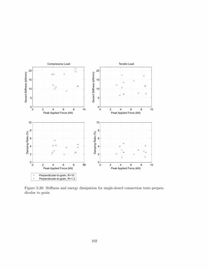
0 2 4 6 8 100
5
10
15
20
Peak Applied Force (kN)
Secant S
tiffness (
kN
/mm
)
Tensile Load
0 2 4 6 8 100
5
10
15
20
Peak Applied Force (kN)
Secant S
tiffness (
kN
/mm
)
Compressive Load
0 2 4 6 8 10
Peak Applied Force (kN)
Dam
pin
g R
atio (
%)
Perpendicular-to-grain, R=10
Perpendicular-to-grain, R=1.2
10
Peak Applied Force (kN)
Dam
pin
g R
atio (
%)
0 2 4 6 8 100
2
4
6
8
10
0
2
4
6
8
10
Figure 5-20: Stiffness and energy dissipation for single-dowel connection tests perpen-dicular to grain
102
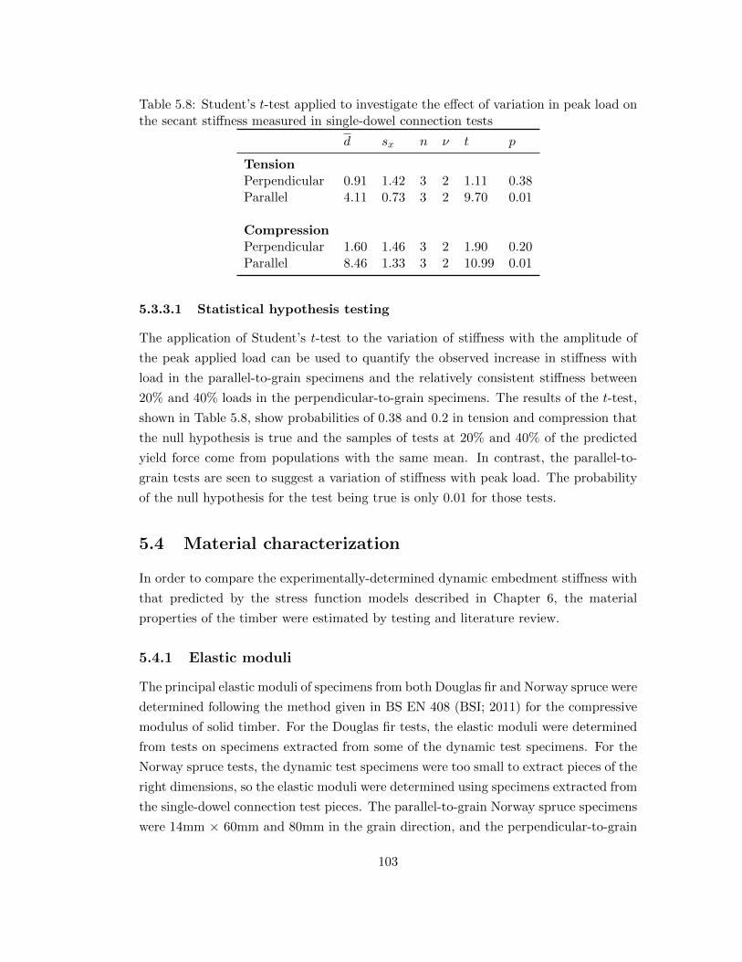
Table 5.8: Student’s t-test applied to investigate the effect of variation in peak load onthe secant stiffness measured in single-dowel connection tests
d sx n ν t p
TensionPerpendicular 0.91 1.42 3 2 1.11 0.38Parallel 4.11 0.73 3 2 9.70 0.01
CompressionPerpendicular 1.60 1.46 3 2 1.90 0.20Parallel 8.46 1.33 3 2 10.99 0.01
5.3.3.1 Statistical hypothesis testing
The application of Student’s t-test to the variation of stiffness with the amplitude of
the peak applied load can be used to quantify the observed increase in stiffness with
load in the parallel-to-grain specimens and the relatively consistent stiffness between
20% and 40% loads in the perpendicular-to-grain specimens. The results of the t-test,
shown in Table 5.8, show probabilities of 0.38 and 0.2 in tension and compression that
the null hypothesis is true and the samples of tests at 20% and 40% of the predicted
yield force come from populations with the same mean. In contrast, the parallel-to-
grain tests are seen to suggest a variation of stiffness with peak load. The probability
of the null hypothesis for the test being true is only 0.01 for those tests.
5.4 Material characterization
In order to compare the experimentally-determined dynamic embedment stiffness with
that predicted by the stress function models described in Chapter 6, the material
properties of the timber were estimated by testing and literature review.
5.4.1 Elastic moduli
The principal elastic moduli of specimens from both Douglas fir and Norway spruce were
determined following the method given in BS EN 408 (BSI; 2011) for the compressive
modulus of solid timber. For the Douglas fir tests, the elastic moduli were determined
from tests on specimens extracted from some of the dynamic test specimens. For the
Norway spruce tests, the dynamic test specimens were too small to extract pieces of the
right dimensions, so the elastic moduli were determined using specimens extracted from
the single-dowel connection test pieces. The parallel-to-grain Norway spruce specimens
were 14mm × 60mm and 80mm in the grain direction, and the perpendicular-to-grain
103

Table 5.9: Douglas fir dynamic test specimens from which elastic modulus specimenswere extracted
Test Grain Peak Force R-ratio No. of
Orientation FpeakFpeakFtrough
Specimens
(% of StaticFailure)
1 Parallel 20% 1.2 22 Parallel 20% 10 23 Parallel 40% 1.2 34 Parallel 40% 10 25 Parallel 80% 1.2 36 Parallel 80% 10 17 Perpendicular 20% 1.2 38 Perpendicular 20% 10 29 Perpendicular 40% 1.2 210 Perpendicular 40% 10 211 Perpendicular 80% 1.2 212 Perpendicular 80% 10 2
Table 5.10: Mean measured elastic moduli and coefficients of variation (COV)
Species Parallel-to-grain Perpendicular-to-grainElastic Modulus COV Elastic Modulus COV
Douglas fir 10569 0.21 322 0.38Norway spruce 12788 0.22 153 0.30
specimens 40mm deep × 70mm in the grain direction and 90mm in the direction in
which the modulus was to be measured.
The Douglas fir specimens for which elastic modulus data were obtained are sum-
marized in Table 5.9. Two specimens were taken from each embedment specimen, one
in each grain direction, so 26 elastic moduli were obtained in each grain direction, 52 in
total. The cutting pattern is shown in Figure 5-21. In the Norway spruce, 18 specimens
were made in each grain orientation, 36 in total.
The tests were carried out using an Instron 20-tonne capacity screw-driven servo
loading machine. A spherical bearing was used to ensure the specimens were loaded
evenly if the top and bottom surfaces were misaligned in manufacture. The deformation
was measured by a pair of extensometers, which ensured that deformation in the contact
surface between the loading head and the specimen and other local effects near the point
of loading were not included in the displacement measurement. The gauge length of the
extensometers was 50mm, and they were located centrally in the height of the specimen.
104

14
4080
8014
40 80
80
All specimens 60mm into page
Figure 5-21: Cutting pattern to extract elastic modulus specimens in each grain direc-tion from the Douglas fir embedment specimens, all dimensions are in millimetres
Extensometer
Lockable sphericalbearing
Figure 5-22: Elastic modulus testing according to EN 408 (BSI; 2011) for a parallel-to-grain Norway-spruce specimen
A parallel-to-grain Norway spruce specimen during testing is shown in Figure 5-22.
The elastic moduli for each species are given in Table 5.10. The coefficient of
variation is higher for the perpendicular-to-grain moduli in each case, due to the fact
that the perpendicular-to-grain specimens included a range of orientations between
radial and tangential. The tangential direction was dominant in the solid planks of
Douglas fir, while the Norway-spruce specimens, taken from glued-laminated timber
beams, contained more specimens with orientations closer to radial.
The measured values of the principal elastic moduli provided two of the four param-
eters required for two-dimensional analytical model. In addition, the Poisson’s ratio
and shear modulus are required. The Wood Handbook (Forest Products Laboratory;
2010) provides mechanical properties for various species of timber grown in the USA
and Canada, including Douglas fir, and Bodig and Jayne (1993) tabulates elastic prop-
105

Table 5.11: Mechanical properties for Douglas fir and spruce - all units are N/mm2,with the exception of the dimensionless Poisson’s ratios
EL ET ER GLR GLT GRT νLR νLT νRT
Douglas fir 14740 737 1002 943 1150 103 0.292 0.449 0.390Spruce 15373 798 503 706 654 36 0.422 0.545 0.470
erties for spruce from three different studies. The values for Douglas fir and Spruce are
summarized in Table 5.11.
In the descriptions of the orthotropic elastic properties by Bodig and Jayne (1993)
and the Wood Handbook (Forest Products Laboratory; 2010), there are nine indepen-
dent elastic constants: three elastic moduli corresponding to the longitudinal, radial
and tangential orientations with respect to the grain and ring structure; three shear
moduli and three Poisson’s ratios. In a single plane, only two elastic moduli, one shear
modulus and one Poisson’s ratio are required.
5.4.2 Estimation of the shear modulus
The mean elastic moduli from the tests on Douglas fir were 10, 569N/mm2 in the
longitudinal direction and 322N/mm2 in the perpendicular direction, which, for most
specimens, was close to tangential. For the Norway spruce, in which the perpendicular
direction was usually close to radial, the mean elastic moduli were 12, 788N/mm2 in
the longitudinal direction and 153N/mm2 in the perpendicular direction. The ratio of
the two moduli in each case was, therefore, quite different from that given in the liter-
ature, since the measured perpendicular moduli were far lower. It was not, therefore,
considered appropriate to obtain the shear modulus as a proportion of the longitudinal
elastic modulus, using a ratio from published results. Another rationale was therefore
sought to estimate the shear modulus.
Jones (1975) shows that if the elastic compliances of an orthotropic material in
plane strain are given by sij , as in (5.15), then the apparent shear compliance, s′66, for
axes at an angle θ to the principal axes, is given by (5.16).
s11 =1
E1s12 =
−ν12E1
s22 =1
G12(5.15)
s′66 =4 (s11 + s22 − 2s12) sin 2θ cos 2θ
+ s66 (sin 2θ − cos 2θ)2(5.16)
106

00
200
400
600
800
1000
Angle (Radians)
G(N
/mm
)1
2
2
π/2 π
Figure 5-23: Variation of apparent shear modulus with angle from the principal direc-tion for Douglas fir
For Douglas fir, as described in the Wood Handbook (Forest Products Laboratory;
2010), the variation of apparent shear modulus with angle in the longitudinal-tangential
plane can be plotted using (5.16). The result is shown in Figure 5-23.
At θ = π/2, s′66 is independent of s66, and so the apparent shear modulus is inde-
pendent of the principal shear modulus. Using the elastic moduli obtained from the
tests, it was therefore possible to calculate the apparent shear modulus at θ = π/2 for
each specimen. The ratio of the maximum and minimum shear modulus from Figure
5-23 was then assumed to apply to the Douglas fir used in the tests, and was used
to estimate the principal shear modulus for each specimen. The same approach was
applied to the Norway spruce.
5.4.3 Friction coefficient
Tests were carried out to estimate the coefficient of friction to use in the analytical
models presented in Chapter 6. Figure 5-24 shows the test setup, in which a vertical
force was applied to two specimens, with a long dowel between. The vertical load
was applied by a servo-hydraulic loading machine, which allowed the load to be held
constant despite any vertical settlement. The dowel was pushed horizontally using a
hydraulic hand jack, and the force required to do so was continuously recorded through
a load cell.
It should be noted that the friction force in this test setup is in a different orientation
to the friction force developed during embedment of the dowel into the timber. Tests by
McKenzie and Karpovich (1968) showed that the grain orientation had no significant
effect on the magnitude of either the static or steady sliding friction coefficients. It was
considered reasonable, therefore, to assume that the frictional behaviour will be similar
in both orientations, so that this test provides a suitable estimate of the coefficient of
107

Normal force appliedby loading machine
Horizontal forceapplied by hand jack
Dowel passesthrough hollowsection
Figure 5-24: Friction test on dynamic test specimens
friction for use in the analytical model. It was noted, however, that the tests on Norway
spruce showed some variation of friction coefficient with grain direction.
Six friction tests were carried out for each species: three with the load applied
parallel to the grain, and three with the load applied perpendicular to the grain. For
the Douglas fir specimens, in each orientation, two specimens were freshly cut, and one
was made from two specimens which had been used for a cyclic embedment test for
1000 cycles at 1Hz, in which the peak load was 40% of the predicted yield force. All the
Norway spruce tests were carried out on freshly-cut specimens. During each friction
test, the normal load was equivalent to 40% of the predicted yield force.
One of the freshly-cut specimens in each grain direction, and in each species, was
used for friction tests at three levels of normal force, to investigate the validity of
the Coulomb friction approximation, which would suggest that the horizontal force to
overcome friction would be proportional to the normal force.
Figure 5-25 shows the plot of applied lateral force against lateral displacement for
one of the friction tests. This highlights the influence of the rate of movement of the
dowel. In part A of Figure 5-25, the lever of the hand jack was pushed down slowly,
which meant that the applied force dropped away before the constant rate of displace-
ment, required for kinetic friction, could develop. The dowel therefore moved a short
distance each time and then stopped, a phenomenon known as stick-slip oscillation.
In part B of Figure 5-25, the lever of the hand jack was moved sufficiently quickly
that kinetic friction could develop, after overcoming the initial, higher force of static
friction. Since there is continuous movement in the dynamic tests, it is considered that
the coefficient of kinetic friction is appropriate as the input to the analytical model.
The coefficient of friction to be used in the model was therefore estimated based on the
kinetic friction in each case.
108
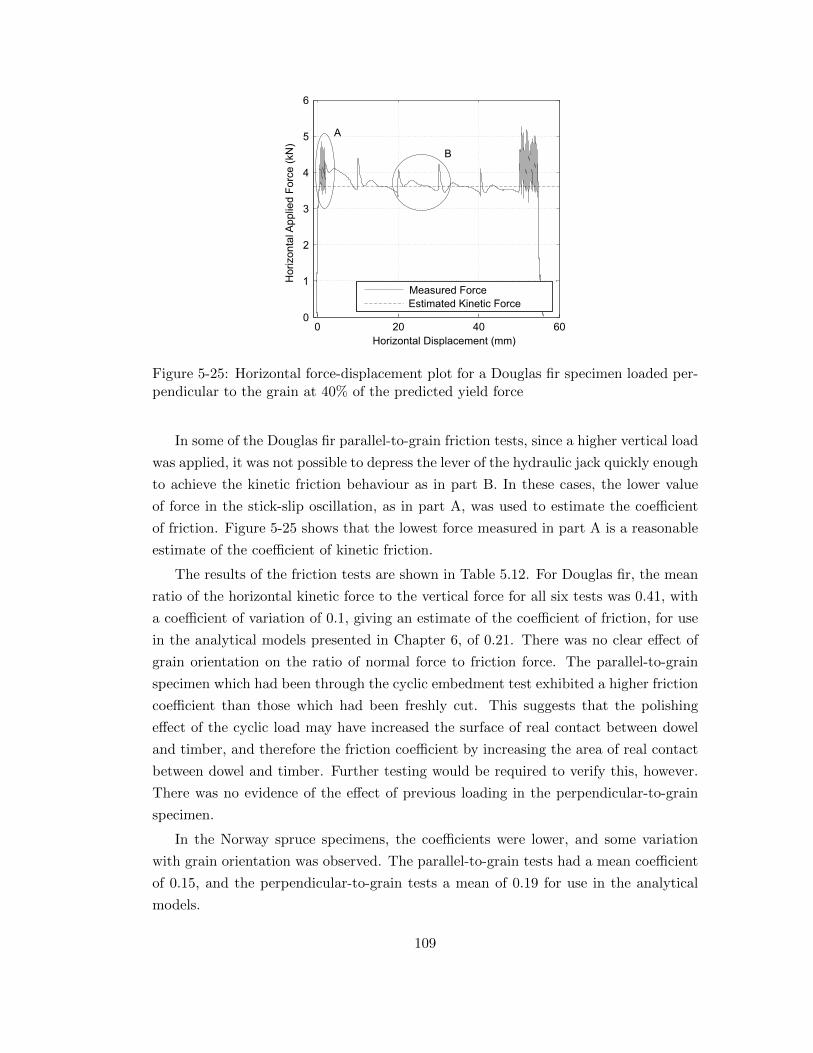
0 20 40 600
1
2
3
4
5
6
Horizontal Displacement (mm)
Horizonta
lApplie
d F
orc
e (
kN
)Measured Force
Estimated Kinetic Force
A
B
Figure 5-25: Horizontal force-displacement plot for a Douglas fir specimen loaded per-pendicular to the grain at 40% of the predicted yield force
In some of the Douglas fir parallel-to-grain friction tests, since a higher vertical load
was applied, it was not possible to depress the lever of the hydraulic jack quickly enough
to achieve the kinetic friction behaviour as in part B. In these cases, the lower value
of force in the stick-slip oscillation, as in part A, was used to estimate the coefficient
of friction. Figure 5-25 shows that the lowest force measured in part A is a reasonable
estimate of the coefficient of kinetic friction.
The results of the friction tests are shown in Table 5.12. For Douglas fir, the mean
ratio of the horizontal kinetic force to the vertical force for all six tests was 0.41, with
a coefficient of variation of 0.1, giving an estimate of the coefficient of friction, for use
in the analytical models presented in Chapter 6, of 0.21. There was no clear effect of
grain orientation on the ratio of normal force to friction force. The parallel-to-grain
specimen which had been through the cyclic embedment test exhibited a higher friction
coefficient than those which had been freshly cut. This suggests that the polishing
effect of the cyclic load may have increased the surface of real contact between dowel
and timber, and therefore the friction coefficient by increasing the area of real contact
between dowel and timber. Further testing would be required to verify this, however.
There was no evidence of the effect of previous loading in the perpendicular-to-grain
specimen.
In the Norway spruce specimens, the coefficients were lower, and some variation
with grain orientation was observed. The parallel-to-grain tests had a mean coefficient
of 0.15, and the perpendicular-to-grain tests a mean of 0.19 for use in the analytical
models.
109

Table 5.12: Friction test results
Normal Static Static Kinetic Kineticforce load coefficient load coefficient(kN) (kN) (kN)
Douglas fir
Para. Unloaded 1 13.8 6.5 0.24 5.4 0.20Para. Unloaded 2 13.8 6.6 0.24 5.2 0.19Para. Loaded 13.8 7 0.25 6.8 0.25
Perp. Unloaded 1 8.4 4.2 0.25 3.3 0.20Perp. Unloaded 2 8.4 4.2 0.25 3.6 0.21Perp. Loaded 8.4 4.2 0.25 3.3 0.20
Norway spruce
Para. Unloaded 1 6.3 2.2 0.17 2.0 0.16Para. Unloaded 2 6.3 2.3 0.18 1.8 0.14Para. Unloaded 3 6.3 2.0 0.15 1.8 0.14
Perp. Unloaded 1 4.1 1.8 0.22 1.7 0.21Perp. Unloaded 2 4.1 1.6 0.19 1.5 0.18Perp. Unloaded 3 4.1 1.6 0.19 1.5 0.18
110

0
1
2
3
4
5
6
7
0 2 4 6 8 10 12 14 16
Horizon
tal F
orc
e(k
N)
Normal Force (kN)
Douglas fir parallel to grain
0
1
2
3
4
0 2 4 6 8
Horizon
tal F
orc
e (
kN
)
Normal Force (kN)
Douglas fir perpendicular to grain
Static
Kinetic
0.0
0.5
1.0
1.5
2.0
2.5
0 1 2 3 4 5 6 7
Horizon
tal F
orc
e
Normal Force (kN)
Norway spruce perpendicular to grain
0.0
0.5
1.0
1.5
2.0
2.5
3.0
3.5
0 1 2 3 4 5 6 7 8 9 10
Horizon
tal F
orc
e
Normal Force (kN)
Norway spruce parallel to grain
Static
Kinetic
Static
Kinetic
Static
Kinetic
Figure 5-26: Measured normal and horizontal forces for initial slip, labelled as static,and constant movement, labelled as kinetic
The effect of variation in the normal force applied to the specimens is shown in
Figure 5-26. It can be seen that the relationship between normal force and horizontal
force is close to linear for both the static and kinetic results. In fact, the coefficient of
determination R2, defined as in Section 2.2.2, is above 0.99 for a linear least-squares
fit of each of the lines. These results help to justify the use of Coulomb friction theory
in the analytical models presented in Chapter 6.
5.5 Microscopy
Microscopy was used to observe the microstructural changes between specimens before
and after loading. The specimens for microscopy were therefore taken from the Douglas
fir embedment specimens, and the plane in which each specimen was cut is shown in
Figure 5-27. The surface of these planes was then viewed under an optical reflected-light
microscope, so the view is along the axis of the tracheids for the perpendicular-to-grain
specimen and along the dowel axis for the parallel-to-grain specimen.
The specimens for microscopy were prepared by cutting followed by sanding with
111

Figure 5-27: Cutting planes for microscopy
0.1mm0.2mm 0.2mm 0.1mm
a b c d
0.2mm
Figure 5-28: Microscope images showing: a parallel-to-grain specimen which has notbeen loaded by a dowel; b parallel-to-grain specimen loaded to a peak load of 40% ofits predicted yield load; c perpendicular-to-grain specimen which has not been loaded;d perpendicular-to-grain specimen loaded to a peak load of 40% of its predicted yieldload
P600 silicon carbide paper. The surface was then cleared of dust with an air jet. In the
case of the perpendicular-to-grain specimen, the air jet did not remove the particles
which had filled the pores, and so a plane surface was created by the cell walls and the
dust filling each pore.
a and c in Figure 5-28 show the microstructure in each orientation for specimens
which had remained unloaded. In the perpendicular-to-grain specimen, the cells appear
to have been undamaged in this plane by drilling and cutting. In the parallel-to-grain
specimens, the tracheids at the edge of the hole curve slightly. This is thought to be a
consequence of either drilling during manufacture, or cutting or sanding during prepa-
ration for microscopy. The fact that all tracheids were observed to curve tangentially
suggests that drilling is the most likely cause.
A similar image for a perpendicular-to-grain specimen which has seen an applied
force 40% of its predicted yield force is shown in d in Figure 5-28. In this specimen,
112

the tracheids near the edge of the hole can be seen to have been permanently crushed.
The process of these tracheids being crushed forms part of the irreversible deforma-
tion which occurs under initial loading. There are also some areas of intact tracheids
around the edge of the hole, which suggests that the crushing of the tracheids acts to
allow force to be distributed to these areas, which may initially have been recessed. It
is thought that the crushing process, therefore, spreads the applied force over a larger
contact area, increasing the stiffness of the connection. Atack and Tabor (1958) noted
this closing of the voids of the trachieds whilst investigating the rolling friction of steel
balls on timber. They also noted that the voids were observed to snap open very quickly
upon addition of a small drop of water. It is considered that it would generally be more
desirable in dowel type connections to increase the initial stiffness of the connection
by causing the crushing of the trachieds before installation of the dowel. It is possible,
however, perhaps for a use in a dedicated energy dissipation device, that it might be
desirable to return the crushed trachieds to their original state, in which case the effect
of the addition of water might be useful.
In the parallel-to-grain specimen, the force is not applied in the direction which
would cause crushing of the tracheids. A similar process of initial irreversible deforma-
tion followed by viscoelastic behaviour occurs, however, and the microscope image in
b in Figure 5-28 shows a possible cause of that initial deformation. In the specimen,
previously loaded to 40% of its predicted yield force, some buckling of the tracheid
walls can be seen, away from the edge of the hole. This buckling is distinct from the
curvature of the tracheids which was observed in the unloaded specimen, in that it
does not occur immediately at the edge of the hole. As with the perpendicular-to-grain
specimen, some undamaged areas were also visible, suggesting that the irreversible de-
formation acts to take up unevenness in the contact face between the dowel and the
timber.
5.6 Summary
The experimental results in this chapter have shown the prominent features of the
behaviour of timber in embedment by a steel dowel under loads representative of in-
service vibration. They have also shown that the non-linear features of the response in
embedment are also apparent in the response of a single-dowel connection.
It has been found that the stiffness and energy dissipation of a dowel-type connec-
tion tend towards a constant value after repeated cycles of load. In the early cycles,
a transient contribution to stiffness and energy dissipation was observed, which was
thought to be due to the deformation occurring in the contact surface between steel
113
and timber. The permanent deformation in that contact surface was observed by com-
paring microscope images from specimens before and after load testing.
In the tests with R=10, substantial non-linear force-displacement behaviour was
observed, while at R=1.2, there was little deviation from a linear-elastic response. This
was thought, again, to be due to deformation in the uneven contact surface and resulted
in a reduced stiffness and an increased energy dissipation at the higher amplitude.
The next chapter will investigate methods of modelling the embedment behaviour
which has been described in this chapter, and relate the embedment behaviour to that
of the single-dowel connections.
114

Chapter 6
Models for Embedment
The behaviour of a dowel-type connection can be understood by first considering the
embedment of the connector into the timber around it, then the deformation of a single
connector along its length, and finally the interaction of groups of connectors under
the applied force and moment. The derivation of a model for connection stiffness and
energy dissipation under in-service vibration therefore addresses each of those processes.
The results presented in Chapter 5 showed that the nonlinear, time dependent and
dissipative behaviour of the connection occurs primarily in embedment. The load-
deflection response of a circular dowel embedding into a piece of timber depends on
the orthotropic elastic behaviour of the timber, and also on the frictional interaction
between the dowel and the timber. An analytical method has been developed to model
the stiffness and energy dissipation of the embedding dowel, which takes into account
these processes, and that method is described in this chapter.
The method was developed on the assumption that, under small-amplitude vibra-
tion significantly below the embedment strength, the behaviour of the timber could
be treated as linear, and therefore modelled using an orthotropic linear elastic model.
The deformation of the cross-section of the steel dowel was assumed to be negligible,
but the friction between the steel and timber determines the distribution of the forces
around the face of the timber, so had to be modelled.
Some of the nonlinear and viscoelastic components of the measured embedment
behaviour were then represented by a rheological model. This model was used as an
inverse-modelling tool to quantify the relative magnitudes of the deformations due to:
the plastic behaviour considered to occur in the contact surface; the elastic deformation
in the timber and the viscoelastic flow in the timber over time. The viscoelastic model
did not form part of the linear elastic method for estimation of connection and frame
stiffness under small-amplitude one-sided cyclic loading, but provided some insight into
115

the field of application of such an elastic model.
Figure 6-1 shows the relationships between all the models developed in this chapter
and Chapter 7.
6.1 Elastic foundation models
Two elastic foundation models are presented, and in each the foundation modulus for
the timber is estimated using a stress function of the form first proposed by Lekhnitskii
(1968). The definition of the stress function then exactly follows the work of Zhang and
Ueng (1984) and Hyer and Klang (1985), and the formulae are collated and reproduced
here for convenience. The work of those researchers is then extended to assess the
deformations in a specimen by superposition of infinite or semi-infinite plate stress
functions.
These are linear-elastic models for the timber, but the interaction between dowel
and timber is nonlinear not just because of the friction between the two, but also
because the timber surface is initially uneven, and this unevenness is compressed under
load, improving the contact surface, as seen in microscopy in Section 5.5. This effect
is discussed by Dorn et al. (2013), who suggested that the low initial stiffness may
be due to the compression of the unevenness in the contact surface, and noted that
under unloading and reloading the embedment behaviour is closer to linear elastic,
as the surface of the timber remains compressed to its previous level. The effect of
unevenness of the contact surface was not taken into account in this elastic model,
meaning that it is appropriate only to the secant stiffness under cyclic loading, in
which the contact surface is assumed to have been compressed to provide a relatively
stiff transfer of load to the timber.
6.1.1 A half hole in a semi-infinite plate
The stress function by Zhang and Ueng (1984) represents the stresses in a semi-infinite
orthotropic plate in plane stress with a half-hole in the surface. The following derivation
of the model, and its comparison with the results of the Douglas fir embedment tests,
were presented in a peer-reviewed publication (Reynolds et al.; 2013a).
The forces applied by the dowel along the surface of the half-hole are defined on the
basis of the geometry and the coefficient of friction between the steel and the timber.
The geometry and notation are shown in Figure 6-2.
Lekhnitskii (1968) showed that the general form of the stress functions for an infinite
orthotropic plate with a hole is as given by (6.2) to (6.6). The solution of a particular
problem relies on finding the coefficients an and bn which correspond to the distribution
116

Elastic stress-functionmodel for dowel-timber
interaction
Beam on foundationmodel for dowel
deformation
Equations for loaddistribution between
dowels
Stiffness matrix withsemi-rigid connections
Foundationmodulus
Individualconnectorstiffness
Connectiontranslationaland rotationalstiffness
Natural frequency offrame
Distribution of elasticwork done in modes
Energydissipation
Damping estimatebased on energydissipation byfriction
Equations for loaddistribution between
dowels
Rheological modelfor embedment
Relative magnitudeof elastic, plastic and
viscoelasticmovement
Figure 6-1: Models for embedment, dowel, connection and frame behaviour, showingtheir relationships to one another
117

Steel
Timber
y
r
x
θ
Figure 6-2: Geometry and notation for stress function model for embedment
of the load on the edge of the hole. ζ1,2 are transformed coordinates describing the
point on the plate under consideration. The complex stress functions and Φ1 and Φ2
are defined so that the displacements u, in the x direction, and v, in the y direction,
are given by (6.7) and (6.8). i is the imaginary unit.
Φ1 and Φ2 are stress functions defined by their relationship to the direct and shear
stresses in the plate: the direct stress in the x direction, for example, is given by (6.1),
where Φ′1 is the derivative of Φ1 with respect to z1, and Φ′2 the derivative of Φ2 with
respect to z2. Re() denotes the real part of what is, in general, a complex number in
the brackets, and µ1 and µ2 are complex constants derived from the material properties
of the plate, as in (6.9) and (6.10).
σx = 2Re(µ1Φ′1 + µ2Φ
′2) (6.1)
This work is not concerned with the stresses in the plate, but rather the relative dis-
placements. The displacements in the plate are given by the integral of the strains, and
are therefore proportional to the integral of the stresses. The displacements are there-
fore calculated using the undifferentiated stress functions Φ1 and Φ2. A full derivation
of the general form of the stress functions and their relationship to stresses, strains and
displacements is given by Lekhnitskii (1968).
Φ1 = a0lnζ1 +
∞∑n=2
anζn1
(6.2)
Φ2 = b0lnζ2 +∞∑n=2
bnζn2
(6.3)
118

ζ1 =z1 +
√z21 −
(1 + µ21
)r2(1− iµ21
) (6.4)
ζ2 =z2 +
√z22 −
(1 + µ22
)r2(1− iµ22
) (6.5)
z1 = x+ µ1y z2 = x+ µ2y (6.6)
u = 2Re (p1Φ1 + p2Φ2) + U (6.7)
v = 2Re (q1Φ1 + q2Φ2) (6.8)
u is the displacement relative to a particular fixed point, and includes one non-zero
constant of integration, U . µ1, µ2, p1, p2, q1 and q2 are derived from the material
properties of the plate material, the timber, as in (6.9) to (6.14), where E1 is the
elastic modulus of the plate material in the x direction, E2 the elastic modulus in the
y direction, G is the shear modulus, and ν12 the Poisson’s ratio in the xy plane.
µ21 =2ν12 − E1
G +√(
2ν12 − E1G
)2 − 4E1E2
2(6.9)
µ22 =2ν12 − E1
G −√(
2ν12 − E1G
)2 − 4E1E2
2(6.10)
p1 =µ21E1− ν12E1
(6.11)
p2 =µ22E1− ν12E1
(6.12)
q1 =1
µ1E2− ν12µ1
E1(6.13)
q2 =1
µ2E2− ν12µ2
E1(6.14)
Lekhnitskii (1968) presented a method to allow the stress functions to be defined
on the basis of the trigonometric series defining the displacements u′ and v′ on the
119
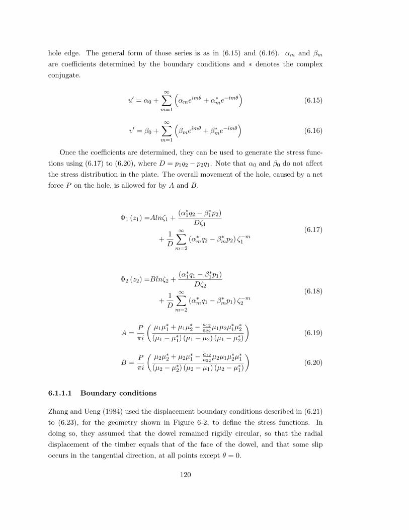
hole edge. The general form of those series is as in (6.15) and (6.16). αm and βm
are coefficients determined by the boundary conditions and ∗ denotes the complex
conjugate.
u′ = α0 +∞∑m=1
(αme
imθ + α∗me−imθ
)(6.15)
v′ = β0 +∞∑m=1
(βme
imθ + β∗me−imθ
)(6.16)
Once the coefficients are determined, they can be used to generate the stress func-
tions using (6.17) to (6.20), where D = p1q2 − p2q1. Note that α0 and β0 do not affect
the stress distribution in the plate. The overall movement of the hole, caused by a net
force P on the hole, is allowed for by A and B.
Φ1 (z1) =Alnζ1 +(α∗1q2 − β∗1p2)
Dζ1
+1
D
∞∑m=2
(α∗mq2 − β∗mp2) ζ−m1
(6.17)
Φ2 (z2) =Blnζ2 +(α∗1q1 − β∗1p1)
Dζ2
+1
D
∞∑m=2
(α∗mq1 − β∗mp1) ζ−m2
(6.18)
A =P
πi
(µ1µ
∗1 + µ1µ
∗2 − a12
a22µ1µ2µ
∗1µ∗2
(µ1 − µ∗1) (µ1 − µ2) (µ1 − µ∗2)
)(6.19)
B =P
πi
(µ2µ
∗2 + µ2µ
∗1 − a12
a22µ2µ1µ
∗2µ∗1
(µ2 − µ∗2) (µ2 − µ1) (µ2 − µ∗1)
)(6.20)
6.1.1.1 Boundary conditions
Zhang and Ueng (1984) used the displacement boundary conditions described in (6.21)
to (6.23), for the geometry shown in Figure 6-2, to define the stress functions. In
doing so, they assumed that the dowel remained rigidly circular, so that the radial
displacement of the timber equals that of the face of the dowel, and that some slip
occurs in the tangential direction, at all points except θ = 0.
120

u =u0cs
and v = 0 when θ = ±π2
(6.21)
u = u0 and v = 0 when θ = 0 (6.22)
(u0 − u) cos θ = v sin θ when−π2≤ θ ≤ π
2(6.23)
u0 is, therefore, the displacement of the dowel in the semi-infinite plate, and cs
represents the extent to which the dowel slips along the surface of the timber. Zhang
and Ueng (1984) proposed the trigonometric series in (6.24) to (6.32) to satisfy these
boundary conditions. Using these boundary conditions, the standard form of stress
function defined by (6.15) and (6.16), the stress functions for this particular case are
defined as in (6.33) and (6.34). It can be seen that the friction coefficient µ affects
the slip cs, since it appears in the equations for the constants A1 and B1, which also
depend on the material properties of the timber.
u′ =c− 1
2csu0 cos 2θ +
c+ 1
2csu0cos4θ (6.24)
v′ =
(cs − 1
2cs+cs + 1
cs
)u0 sin 2θ +
cs + 1
2csu0sin4θ (6.25)
cs =B1 −A1
A1(6.26)
u0 =gP
π
(B1 −A1)
2A1 (ν12 − k − nk)−B1 (ν12 − k − nk)(6.27)
A1 = (19n+ 11nk + 10k − 10ν12)
+ µ (11n− 6nk + 15k − 15ν12)(6.28)
B1 = 10n (1− k) + 10µ (3k − 3ν12 + 2nk + n) (6.29)
k =
√E1
E2(6.30)
n =
√2 (k − ν12) +
E1
G(6.31)
121

6040200-20-40-60
0.2
0.1
0
-0.1
-0.2
Shear
str
ess o
ver
peak d
irect str
ess
Distance from hole centre(mm)
μ=0.1
μ=0.2
μ=0.4
μ=0.8
Shear force plotted
Timber
Figure 6-3: Shear on the free surface in the approximate solution for a semi-infiniteplate (Zhang and Ueng; 1984)
g =1− ν212E2
E1
E2+k
G(6.32)
Φ1 = A ln ζ1 +
(cs − 1
2x
q2 − ip22D
− cs + 1
cs
ip22D
)u0ζ21
+cs + 1
2cs
q2 − ip22D
u0ζ41
(6.33)
Φ2 = B ln ζ2 +
(− (cs − 1)
2x
q1 − ip12D
+cs + 1
cs
ip12D
)u0ζ22− cs + 1
2cs
q1 − ip12D
u0ζ42
(6.34)
Although the general solution by Lekhnitskii (1968) is for a hole in an infinite
plate, the form of the stress functions proposed by Zhang and Ueng (1984) means that
the vertical component of the resultant force applied to the plate is zero on the y-
axis. These functions therefore approximate a semi-infinite plate with a half-hole. It is
convenient that this is appropriate for the geometry in the embedment tests described
in Section 5.
It should be noted that this is only an approximate solution for a semi-infinite plate
with a half-hole, because the shear stress on the y-axis is not zero. Zhang and Ueng
(1984) state that this approximation does not affect the stress field significantly for
low friction coefficient, and on that basis, it is assumed that it will not significantly
affect the vertical deformations. Figure 6-3 plots the shear stress on the free surface
for a range of friction coefficients for the mean material properties of the Douglas fir,
showing that it exceeds 10% of the peak compressive stress for a friction coefficient of
0.4 or greater.
122

h
Superposition createsa line along which thedisplacement is zero
Superimposedsecond solution
Geometry tobe modelled
y
x
Figure 6-4: Superposition of two infinite-plate solutions to model a supported edge
A further approximation is inherent in the number of terms used in the equations
to describe the boundary conditions. Further terms could give a more accurate repre-
sentation of the offset position of the dowel. The accuracy of the stress function in this
form will be considered in comparing analytical and experimental results in Section
6.4.
6.1.1.2 Superposition for displacements
The movement of the dowel for a particular applied load, and particular support con-
ditions, will, in general, be different from the deformation u0. The strain field is
integrated to give the deformations in the plate, resulting, for this case, in one non-
zero constant of integration, U in (6.24). For the case of the ASTM embedment test,
the constant was eliminated by superimposing the solutions for two holes loaded in
opposite directions. By placing the second 2h below the first, as shown in Figure 6-4,
a line of zero displacement is created at a vertical distance h from the hole. If the
holes are sufficiently well separated that there is no significant interaction between the
stresses on the edges of each hole, then this is a reasonable representation of a plate
supported rigidly along one edge.
In order to calculate the movement of the dowel, the displacement of the timber
in the semi-infinite plate is calculated in two positions, u0 at y = 0, x = r and u1 at
y = 0, x = 2h− r. u0 can be calculated directly using (6.27). For u1, the transformed
coordinates ζ1 and ζ2 are calculated using (6.4) and (6.5). Since the point is on the
x-axis, ζ1 and ζ2 are equal in both cases. Φ1 and Φ2 are then calculated using (6.33)
123

and (6.34), for a unit applied force P . u1 is then calculated using (6.7).
The displacement of the dowel relative to the fixed surface at x = h is then given
by u1−u02 , and the predicted stiffness of the specimen can be calculated as 2
u1−u0 .
6.1.2 A complete hole in an infinite plate
The complex stress function by Zhang and Ueng (1984) and its extension therefore
give a model suitable for the embedment test geometry. Furthermore, it was argued in
Section 2.2.1 that the effect of the presence of the timber on the unloaded side of the
hole on the foundation modulus measured in these standard embedment tests is small
in comparison to the natural variation of the material properties. In certain geometries,
however, the semi-infinite plate solution appears to be inappropriate: where a timber
member is subject to a tensile force applied by the dowel, for example, or where two
or more dowels exert a couple to resist a bending moment.
The Fourier series representing the force or displacement on the hole edge for a
complete hole needs to contain more terms than the two used by Zhang and Ueng
(1984) to model the half-hole. Hyer and Klang (1985) developed a general solution for
the infinite Fourier series to fully represent the distribution of normal and shear forces
on the hole edge.
6.1.2.1 Boundary conditions
In contrast to the semi-infinite plate model described in Section 6.1.1, which was defined
using only displacement boundary conditions, the calculation for a complete hole in
an infinite plate requires both displacement and force boundary conditions. This is
particularly due to the fact that on the unloaded face of the hole, the displacement
can take any value, while the normal and tangential force on the face of the timber is
known to be zero. The boundary conditions are, therefore, defined for three regions
around the face of the dowel, referred to as the stick, slip and no-contact regions and
shown in Figure 6-5.
In the stick region, the tangential force between timber and dowel is less than the
static friction force, so the two move together. A displacement boundary condition is,
therefore applied in this region, as in (6.35), where u and v are the deflections of the
timber in the x and y directions and u0 is the displacement of the dowel.
u = u0 v = 0 (6.35)
In the slip region, the faces remain in contact, but the tangential force has overcome
the static friction force, so that the two faces have moved relative to one another. As
124

Steel
Timber
y
xStick
Slip
No contact
Figure 6-5: The stick, slip and no-contact regions for the boundary conditions aroundthe hole edge
shown in (6.36), displacement and force boundary conditions are applied here, stating
that the radial displacement in the timber ur is equal to that of the dowel, and assuming
that the tangential force T is equal to the static limiting friction force, given as the
normal force N multiplied by the coefficient of friction µ. The displacement condition
here is a simplification which applies for small displacements, and was used by Zhang
and Ueng (1984) and Hyer and Klang (1985), though neither acknowledged that it was
a simplification. The true relationship between the radial displacement of the timber
and the dowel displacement can be derived based on the fact that the final position
each timber element must fall on the circle defined by the new position of the dowel,
and is given by (6.37).
(6.37), however, since it is not a linear function of ur and uθ, does not obey the
principle of linear superposition which is necessary for Hyer and Klang’s method for
determining the forces on the hole edge. Since the same method is used here, the same
simplification of the boundary condition, given by (6.36), is used.
ur = u0 cos θ N + µT = 0 (6.36)
−(1 + ur)cos(θ + uθ) +√
(2(1 + ur)cos(θ + uθ))2 − 4((1 + ur)2 − 1)
2= u0 (6.37)
In the final region, representing the rest of the face of the timber, it is assumed that
there is no contact between the steel and the timber. Two force boundary conditions
are therefore applied here, reflecting the fact that the normal and tangential forces on
the timber are zero, as in (6.38).
125

T = 0 N = 0 (6.38)
6.1.2.2 Generating the Fourier series for applied force
The general solution by Lekhnitskii (1968) is a stress function for an infinite orthotropic
plate in plane stress, with a hole loaded on its edge. Hyer and Klang (1985) applied
the general complex Fourier series (6.39) to the plate, and related the values of the
coefficients an and bn in (6.2) to (6.6) to the Fourier coefficients by equating the forces
at the hole edge, giving (6.40). δ1,2 and γ1,2 are material properties defined by (6.41).
µ1,2 in (6.41) are the two roots of the characteristic equation for the stress state in
the material (2.5), and so describe the material properties of the plate material. For
the elastic constants of timber, the real part of the complex material properties µ1,2 is
zero. The imaginary parts of δ1,2 and γ1,2 are therefore zero.
n=∞∑n=−∞
Aneinθ (6.39)
n=∞∑n=−∞
Aneinθ = δ1
(a0e−iθ −
∞∑k=1
kane−i(k+1)θ
)+ δ2
(b0e−iθ −
∞∑k=1
kbne−i(k+1)θ
)
− γ1
(a0e−iθ −
∞∑k=1
kanei(k−1)θ
)− γ2
(b0e−iθ −
∞∑k=1
kbnei(k−1)θ
)(6.40)
δ1 =1 + iµ1
2δ2 =
1 + iµ22
γ1 =1− iµ1
2γ2 =
1− iµ22
(6.41)
Hyer and Klang (1985) used the orthogonality of the sinusoidal functions on each
side of (6.40) to evaluate the relationship between the An coefficients and the an and bn.
This process can be carried out for all the coefficients in the complex stress function,
an and bn and, in general, the coefficients are as follows: for c ≤ −2, if Ac = 1 and all
other An = 0, the non-zero an and bn are given by (6.42). For c ≥ 0, if Ac = 1 and all
other An = 0, the non-zero an and bn are given by (6.43).
126
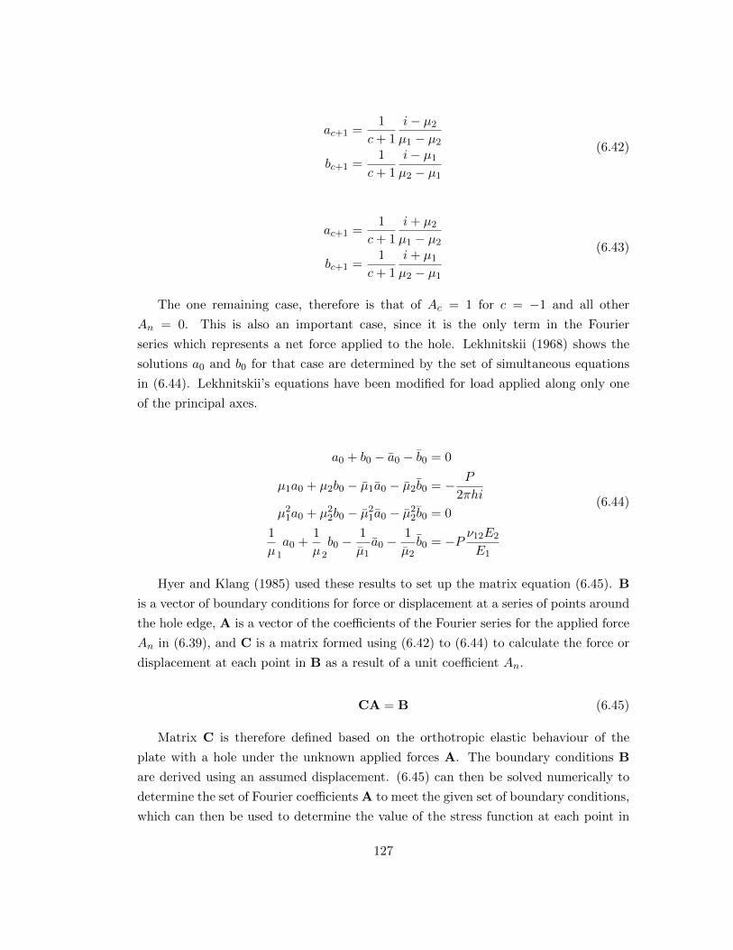
ac+1 =1
c+ 1
i− µ2µ1 − µ2
bc+1 =1
c+ 1
i− µ1µ2 − µ1
(6.42)
ac+1 =1
c+ 1
i+ µ2µ1 − µ2
bc+1 =1
c+ 1
i+ µ1µ2 − µ1
(6.43)
The one remaining case, therefore is that of Ac = 1 for c = −1 and all other
An = 0. This is also an important case, since it is the only term in the Fourier
series which represents a net force applied to the hole. Lekhnitskii (1968) shows the
solutions a0 and b0 for that case are determined by the set of simultaneous equations
in (6.44). Lekhnitskii’s equations have been modified for load applied along only one
of the principal axes.
a0 + b0 − a0 − b0 = 0
µ1a0 + µ2b0 − µ1a0 − µ2b0 = − P
2πhi
µ21a0 + µ22b0 − µ21a0 − µ22b0 = 0
1
µ1
a0 +1
µ2
b0 −1
µ1a0 −
1
µ2b0 = −P ν12E2
E1
(6.44)
Hyer and Klang (1985) used these results to set up the matrix equation (6.45). B
is a vector of boundary conditions for force or displacement at a series of points around
the hole edge, A is a vector of the coefficients of the Fourier series for the applied force
An in (6.39), and C is a matrix formed using (6.42) to (6.44) to calculate the force or
displacement at each point in B as a result of a unit coefficient An.
CA = B (6.45)
Matrix C is therefore defined based on the orthotropic elastic behaviour of the
plate with a hole under the unknown applied forces A. The boundary conditions B
are derived using an assumed displacement. (6.45) can then be solved numerically to
determine the set of Fourier coefficients A to meet the given set of boundary conditions,
which can then be used to determine the value of the stress function at each point in
127

Edge distancesufficient that strainfield is not significantlyaffected
Equal forces inopposite directionsresist a moment appliedsufficiently far away
Figure 6-6: Superposition of two infinite-plate solutions to represent two dowels forminga couple
the plate and so the distribution of stress, strain and displacement.
6.1.2.3 Superposition for displacements
The solution can then be translated and superimposed to calculate relative displace-
ments between dowels. This method is effective when, as in the case of the ASTM
D5764 (ASTM; 1997) or EN 383 (BSI; 2007) embedment tests, the free edges of the
timber do not significantly affect the distribution of stress. This could also be said to
be the case for calculation of the rotational stiffness of a moment connection, where
the timber subject to significant stress is between the dowels forming the couple. The
superposition for two dowels forming a couple is shown in Figure 6-6.
An example of a geometry in which the free edges of the timber affect the stress
distribution is the single-dowel connection test, described in Section 5.2.2. In the
infinite-plate solution, the stresses tend towards zero far from the dowel. In the single-
dowel connection test, the effect of the edges of the timber is to concentrate the stress,
so it tends towards a constant value across the section width w of P/tw, where P is
the force applied to the dowel, and t is the thickness of the timber.
One way to account for this effect is to superimpose the solution for a stretched
plate with a hole onto the pin-loaded plate solution. The infinite plate with a hole
loaded along its edge creates a stress field with compressive stresses on the loaded side
of the dowel and tensile stresses on the unloaded side, so that, by symmetry, half of the
dowel force is resisted in tension and half in compression. By imposing a far-field tensile
stress giving half the force on the dowel spread over the cross section, as presented by
Echavarrıa et al. (2007), the stresses on the loaded side of the dowel approximately
128

cancel out, and the stresses on the unloaded side add to give a tensile force equal to the
load on the dowel. Hence the arrangement approximates a dowel transmitting tensile
force to a timber beam, and the equivalent situation for a compressive force can be
achieved using a compressed, rather than a stretched plate superposition. Echavarrıa
et al. (2007) used the arrangement to investigate the stress around the dowel. The
stresses further along the beam will become inaccurate, however, since the integral of
the stress over the cross section tends towards only half of the applied load on the
dowel.
The general form of the stress function for a pin-loaded stretched plate, subject to
a uniform tensile stress of p, is given by (6.46).
φ1 = a0 ln ζ1 +p
2
((−i
µ1 − µ2
)1
ζ1+
z1µ21 − µ22
)+
∞∑n=1
anζn1
φ2 = b0 ln ζ2 +p
2
((−i
µ2 − µ1
)1
ζ2+
z2µ22 − µ21
)+∞∑n=1
bnζn2
(6.46)
In contrast to the work by Echavarrıa et al. (2007), this study is concerned with the
movement of the connector relative to other connectors or supports. For that purpose,
the stress function in (6.46) can be broken down into three parts:
• the terms in 1/ζn1,2 represent the change in shape of the hole itself, none of them
applying a net force to the hole boundary, so that their effect is confined to the
area immediately around the connector;
• the term in lnζ1,2 represents the net force applied to the hole edge, causing a
concentrated stress in the timber member and the movement of the hole through
the timber; and
• the term in p represents the constant value towards which the stress in the member
tends, far from the hole.
The edge distances required in timber connections to prevent splitting by Eurocode
5 (BSI; 2009a) ensure that edge effects do not significantly change the local stresses
and strains around the hole described by the 1/ζn1,2 terms, so they present a reasonable
model of the deformed shape of the hole. Figure 6-7 shows the direct stresses due to the
1/ζn1,2 terms, in the direction of the applied load, for a piece of timber loaded parallel
to grain with standard C24 material properties according to EN 338 (BSI; 2009b).
The extents of the plot are the minimum edge distances according to Eurocode 5 (BSI;
2009a), 7 times the diameter in the along-grain direction and four times the diameter in
129

-5
0
5 -5
0
5
-2
-1.5
-1
-0.5
0
0.5
x/dy/d
σx/(
P/d
)
2
1
0
-1
-2
Figure 6-7: Stresses in the timber due to the 1/ζn1,2 terms, in which the stress has beennormalized by the dowel force P divided by the diameter d, x is the coordinate in theloading direction and y is the coordinate perpendicular to the load
the across-grain direction, and it can be seen that the stresses diminish rapidly before
the edge of the timber. The highest residual stress at the edge is approximately 1.5%
of the peak.
The longitudinal stress in a long member in tension or compression will tend towards
being evenly distributed across the cross section, with magnitude P/(tw), where t and
w are the dimensions of the beam cross section, and P is the force applied to the
dowel. In the infinite plate solution, the force on the dowel is resisted by the stress in
the material on the loaded and unloaded sides of the dowel, and the integral of that
stress tends towards P/2 on each side. As noted by Echavarrıa et al. (2007), therefore,
a stress in the plate of P/2 is required to cancel out the stress on one side of the dowel,
and approximate a dowel supported on just one side. When two of these infinite plate
solutions are superimposed, therefore, the stress between the dowels tends towards
P/(tw). This is considered to be a suitable approximation of the stress state between
the dowels for calculation of their relative deformations.
The parallel-to-grain single-dowel connection test described in Section 5.2.2 was
used as an example. Two infinite-plate solutions, including the stretched-plate terms,
were superimposed to give the stress function for the geometry in the test. The resulting
deformation field is shown in Figure 6-8.
It should be noted that the calculation illustrated in Figure 6-8 gives a higher
stiffness between the two dowels in the case where they transmit a compressive load
than in the case where they transmit a tensile load. This is due to the longer load path
in the tensile case, in which the load is transmitted in concentrated tension and shear
130

Figure 6-8: Field of deformation in the x direction for single dowel specimens in tensionand compression
either side of the hole. The difference is approximately 5% of the total stiffness in this
case, but its magnitude will depend on the geometry of the particular connection. It
is considered unlikely that a normal structural engineering design process could take
this difference into account, but it is notable nonetheless, and reflects the results of the
single dowel connection tests reported in Section 5.2.2.
The stiffness between the two dowels calculated from the superposition of stress
functions was used as the foundation modulus in a beam-on-elastic-foundation model
for the complete dowel. It is pertinent at this point to discuss the assumption of plane
stress inherent in the stress function model. The plane stress assumption is appropri-
ate where the body being considered is subject to uniform applied force throughout its
thickness, is relatively thin and unconstrained on each face. This geometry meets the
requirement of being unconstrained on each face. Its thickness is, however, of the same
order of magnitude as the hole diameter, and the applied force is not constant through-
out the thickness. The conditions are more suited to the condition of plane stress than
plane strain, however, the latter representing a structure very long in the out-of-plane
direction, or rigidly restrained at its ends, and commonly applied to structures such as
retaining walls.
For the intermediate condition represented by the dowel-type connection, the plane-
stress assumption provides an underestimate, and plane strain an overestimate of the
true stiffness. The alternative to these simplifying assumptions is a three-dimensional
solution which, to the knowledge of the author, could only be carried out numerically,
sacrificing the computational simplicity that this analytical solution presents. It is
therefore considered that the underestimate, usually conservative in structural engi-
neering design, is the preferable choice.
131

6.1.2.4 Dimensional analysis
The foundation modulus for the dowel should be expressed in units of force divided
by length squared, since it represents a stiffness per unit length of the connector. The
solution by Hyer and Klang (1985) is for a hole of unit radius and unit plate thickness,
so must be scaled to reflect the real geometry.
To find the foundation modulus given a particular arrangement of dowels, the stress
functions for a unit radius are superimposed, and the relative displacements δ are
calculated for an applied force F . The displacement has units of length, and the
applied force has units of force divided by length, since it is applied to a unit plate
thickness. The model should have the correct relative dimensions, i.e. the distance
between holes as a multiple of the hole radius should match the full-scale geometry to
be modelled.
In order to scale the model to match the full-scale geometry, all the dimensions
would be multiplied by the full-scale radius of the hole. Since the plate has unit
thickness, the stress σ at each point in the plate is proportional to the force divided by
the radius, as in (6.47). As a result, as the radius increases, the stress decreases, and
so does the strain ε.
σ ∝ F
rε ∝ F
r(6.47)
The displacement, u, of any point relative to another is proportional to the strain
times the distance between them. The distance between any two points, since the model
matches the full-scale geometry, is proportional to r. This means that the displacement
between any two points is independent of r, and therefore does not change as the model
is scaled, as given in (6.48).
u ∝ ε× r ∴ u ∝ F (6.48)
Since the relative displacement between two points is independent of r, and depends
only on F , the displacement under a given force, and therefore the stiffness, can be
calculated using the stress function model with unit radius. Given that the model has
a unit plate thickness, this stiffness represents the foundation modulus required for a
beam-on-elastic-foundation model.
This result has the consequence that an embedment specimen, for example, 40mm
high with an 8mm dowel would be expected to have the same stiffness as one 100mm
high with a 20mm dowel, if they were to have the same thickness.
132

-5
0
5
10
15
Deflection (
m)
μ
With shear deformation
Without shear deformation
185mm
Maximum error 4.5%
1kN applied force
Figure 6-9: Deformed shape of a 12mm steel dowel using a beam-on-elastic-foundationmodel with 140N/mm2/mm foundation modulus, with and without shear deformation
6.2 Beam on foundation
All the foregoing discussion and analysis considers only the embedment behaviour of
the dowel in the timber, which corresponds to the embedment tests in which the dowel
was held rigidly straight as it was pressed into the timber. In any real connection,
there is some deformation of the dowel, and this will be represented by a beam-on-
foundation model, in which the resistance of the timber to embedment is represented
by a foundation modulus and the dowel by a beam to which the appropriate loads
are applied. Since the steady-state cyclic embedment behaviour under the smaller-
amplitude R=1.2 loads is shown, in Section 6.4.2, to be represented well by a linear
elastic model, the foundation provided by the timber will be considered as elastic.
For the connections with a central flitch plate used in this study, the deflection
which defines the connection stiffness is at the centre of the beam, where the load is
applied. Analytical solutions exist for this geometry, both including and excluding shear
deformation. The deformed shape of the dowel for the geometry of the parallel-to-grain
single-dowel connection described in Section 5.2.2 is shown in Figure 6-9, illustrating
the influence of shear deformation for this case.
6.3 Design method for cyclic stiffness
Both the stress function and the beam-on-elastic foundation calculations introduced in
the previous sections reasonably require a computer for their calculation. To be used in
structural engineering design, they could be combined into a simple piece of software,
but it is considered that they would be more useful and intuitive, and appropriate for
integration into design codes, if they were simplified so that they could be used for
133

hand calculation.
For that purpose, the division of the stress function solution into parts is conve-
nient. The part of the stress function which represents the change in the shape of the
hole was seen in Section 6.1.2 to dissipate quickly with distance from the hole. The
edge-distances and spacing required to prevent splitting therefore ensure that the fi-
nite extent of the timber member does not significantly affect this part of the stress
function in parallel-to-grain loading. As a result, this component of the stiffness can
be considered to be a property of the timber, in the same way as Kser is in Eurocode
5. The calculation process can therefore be greatly simplified by tabulating this value
for each timber grade. This component of deformation will hereafter be referred to as
the hole-shape component.
The part of the stress function which represents the far-field stress is only necessary
in cases where edge effects lead to the development of a constant stress in the distance
between the dowels, such as in the linear single-dowel connection considered in this
study. In that case, the effect of this constant stress is simply to produce a constant
strain in the member, and this is considered in a normal frame analysis, independently
of the connections. In calculating the semi-rigid connection stiffness for frame analysis,
therefore, this component of deformation can be omitted.
If the hole-shape component is tabulated, and the far-field stress omitted, then only
one term remains in the equation for the stress function. It represents the movement
of the circular hole relative to the timber around it, which will hereafter be referred to
as the rigid-insert component, since it represents the stress function for the movement
of the hole whilst held rigidly circular. The stress functions Φ1 and Φ2 for this term
are given in (6.49), and are then used to find the displacement in the x-direction by
(6.50). l is the distance between the connections as a multiple of the hole diameter.
The relative displacement between two dowels separated by a distance l is therefore
given by (6.51) to (6.53), which can be combined and simplified to give the approximate
solution (6.54).
Φ1 = a0lnζ1 Φ2 = b0lnζ2 (6.49)
u = 2Re (p1Φ1 + p2Φ2) (6.50)
u0 − ul = −2P
(p1a0ln
ζ1,0ζ1,l
+ p2b0lnζ2,0ζ2,l
)(6.51)
134

ζ1,0ζ1,l
=1 + iµ1
2µ1l +√
4µ1l2 − 1 + (iµ1)2
(6.52)
ζ2,0ζ2,l
=1 + iµ2
2µ2l +√
4µ2l2 − 1 + (iµ2)2
(6.53)
u0 − ul = −2P
(p1a0ln
1 + iµ14l
+ p2b0ln1 + iµ2
4l
)(6.54)
In developing a set of equations suitable for hand calculation, it is considered im-
portant to avoid the use of complex numbers. Since µ1 and µ2 are purely imaginary
quantities, p1a0, p2b0, iµ1 and iµ2 are four real-valued material properties which de-
scribe the orthotropic elastic behaviour of the timber, and can be calculated from its
four independent elastic properties: the two elastic moduli, the shear modulus and the
Poissons ratio. Relabeling p1a0 = β1, p2b0 = β2, iµ1 = α1 and iµ2 = α2, the four
properties are given by (6.55) to (6.58).
α1 =
√√√√ E1G − 2ν12 +
√(2ν12 − E1
G )2 − 4E1E2
2(6.55)
α2 =
√√√√ E1G − 2ν12 −
√(2ν12 − E1
G )2 − 4E1E2
2(6.56)
β1 =1
π
α1(1 + ν12E2E1
α22)
2(α21 − α2
2)
(α21
E1+ν12E1
)(6.57)
β2 =1
π
α2(1 + ν12E2E1
α21)
2(α22 − α2
1)
(α22
E1+ν12E1
)(6.58)
Using these properties, the stiffness associated with the rigid-insert displacement
can then be represented as kf,r in (6.59).
kf,r =1
2(β1ln
1+α14l + β2ln
1+α24l
) (6.59)
The same process can be used for a moment connection. In this case, the second
superimposed stress function is shifted in the direction perpendicular to the applied
load, and so the transformed coordinates ζ1,l and ζ2,l change to reflect that. l is now
the distance between the two connectors as a multiple of the hole diameter, and the
component kf,r of the rigid-insert foundation modulus is given by (6.60).
135

kf,r =1
2(β1ln
1+α14lα1
+ β2ln1+α24lα2
) (6.60)
The foundation modulus for use in a beam-on-elastic foundation model can then be
calculated by combining the stiffness associated with the hole-shape component kf,s,
which could be tabulated, with the rigid-insert stiffness kf,r, which depends on the
geometry of the structure and connection, as in (6.61).
kf =
(1
kf,r+
1
kf,s
)−1(6.61)
The complex stress function model gives an estimate of the stiffness of the timber in
embedment in each plane along the length of the dowel. This stiffness was then used as
the foundation modulus for a beam-on-elastic-foundation model of the complete dowel.
The geometry of the dowel in either a linear or moment connection with a central flitch
plate could be simplified to be represented as a beam on elastic foundation with a
central point load.
The beam-on-elastic-foundation model can be simplified by neglecting shear defor-
mation, which, for the parallel-to-grain single-dowel connection test, can be seen in
Figure 6-9 to represent approximately 5% of the total deflection. This can be con-
sidered to be a representative example in that the relative dimensions of the timber
member and the dowel have been chosen so that the dowel is just slender enough to
give a failure mode with three plastic hinges: failure mode F according to the Euro-
pean Yield Model (BSI; 2009a). Eurocode 5 states that this failure mode is necessary
to ensure plasticity of the connection, which suggests that a well-designed connection
is likely to have this failure mode, and that connections should not generally have a
significantly less slender dowel. It is therefore considered unlikely that the effect of
shear deformation will exceed 6 or 7% in practical timber connections.
Another simplification can be made based on the dowel being relatively long and
slender, since, for a long beam, the deformation at the centre tends towards u0 in
(6.62), which is a widely stated formula. Eb is the elastic modulus of the dowel, P is
the applied force and kf is the foundation modulus determined from the embedment
behaviour of the timber.
u0 =P
d(πEbk
3f
) 14
(6.62)
The design method for connection stiffness under one-sided in-service vibration
therefore consists of:
136
• calculating the transformed material properties from (6.55) to (6.58);
• calculating the rigid-insert stiffness kf,r according to (6.59) for a linear applied
force or (6.60) for a moment;
• reading a tabulated value of the hole-shape stiffness kf,s for a particular grade of
timber;
• combining these stiffnesses according to (6.61) to obtain the foundation modulus
for the beam on elastic foundation; and
• using (6.62) to calculate the stiffness of the individual connector.
Once the stiffness of the individual connector is known, conventional design methods
can be used to assess the semi-rigid connection stiffness for use in a frame analysis for
modal properties.
6.4 Comparison with experimental results
The predictions of this elastic model were compared with the experimental results of
the embedment and single-dowel connection tests presented in Chapter 5 using the
material properties given in Section 5.4.
The two elastic moduli were obtained from tests according to EN 408 (BSI; 2011),
the Poisson’s ratio for the longitudinal-tangential plane was taken from published re-
sults (Bodig and Jayne; 1993; Forest Products Laboratory; 2010), and the shear mod-
ulus was estimated based on the results of the modulus tests and published values, as
described in Section 5.4.2. These properties of the timber were used to create a set
of analytical models for the dynamic test specimens. Using these material properties
and applying a unit force, the value of the two stress functions could be calculated at
each point in the specimen. Using the stress functions, the displacement of every point
in the specimen can be calculated. Those displacements are plotted, for illustrative
purposes, in Figure 6-10.
No free edge effects are allowed for on the sides of the specimen. The edge distances
are considered to be sufficient that the other free edges will not significantly influence
the stress or deformation fields. This simplification will not always be appropriate in
modelling a connection in a structure, and this issue is addressed in Section 6.1.2.
The friction coefficient influences the unrealistic shear force on the free surface
predicted by the stress function, described in Section 6.1.1.1. Based on the measured
coefficient of friction of 0.21, the unrealistic shear stress on the free surface will be less
than 10% of the peak compressive stress for this model, and the effect of that shear
137

0.01
0.02
0.03
0.04
0.05
0.06
Figure 6-10: Vertical displacements in mm in the timber for a typical Douglas firspecimen in parallel-to-grain loading (1kN applied force)
stress on the vertical deformations in the timber beneath the dowel is expected to be
far lower.
The sensitivity of deformation to friction coefficient was assessed by varying the co-
efficient between the extremes of values published by McKenzie and Karpovich (1968),
from their study of friction between steel and timber. For comparison with their work,
the rate of movement between the surfaces in these tests corresponds to their classi-
fication ‘slow’, and the surface of the steel dowel falls between his classes of ‘rough’
and ‘smooth’. For all the species of timber tested, the friction coefficient in these
classifications ranged from 0.08 to 0.62. Using the material properties for one of the
parallel-to-grain Douglas-fir cyclic embedment test specimens, the sensitivity analysis
is summarized in Table 6.1, comparing these extreme values to the mean value obtained
from the friction tests and used in analysis, 0.21. The resulting variation in stiffness is
small in comparison to the variability in material properties in the timber. It is, there-
fore, considered that the sensitivity of stiffness to friction coefficient is not sufficient to
justify a more extensive investigation of friction than has already been carried out.
6.4.1 Statistical hypothesis testing
The modelled stiffness was compared numerically with the experimental results using
either a one-sample or two-sample Student’s t-test. As described in Section 5.2.4,
these tests estimate the probability that two series of tests are two samples taken from
the same population of possible test results. In the context of this chapter, the tests
138

Table 6.1: Effect of friction coefficient on modelled stiffness
Friction Stiffness % ChangeCoefficient from µ = 0.21µ (kN/mm)
0.08 106.2 3.9%0.21 110.5 -0.62 120.8 9.3%
represent a measure of the accuracy of the prediction by the theoretical model which
allows for both the difference in the mean values of experimental results and prediction
and the variance of the measurements.
In order to apply the test, the null hypothesis should first be stated. That is the
hypothesis that the mean stiffness predicted by the model is equal to the mean of the
population from which the experimental tests are taken. A high probability therefore
suggests that the model corresponds well to the experimental results.
For the two-sample t-test, the equations for the test statistic t for independent and
paired samples are as given in Section 5.2.4. In the one-sample t-test, the prediction
is represented just by its mean value, and not by a variance. The equation for the test
statistic t is then given by (6.63), where x is the mean of the test results, µ0 is the
predicted mean, sx is the standard deviation and n the number of tests. The number
of degrees of freedom ν, used to generate the probability density function as in Section
5.2.4, is n− 1.
t =x− µ0
sx√n
(6.63)
6.4.2 Embedment
For the Douglas fir embedment tests analytical results were compared with the experi-
mental results for each grain orientation, and for each R-value. The predicted values of
stiffness are independent of the magnitude of the force applied due to the assumption
of elastic behaviour. The results for the three values of peak force were, therefore,
combined for this comparison of predicted and measured stiffness. Figure 6-11 plots
the stiffness calculated from the experimental results and the analytical model, with
the results organized by grain orientation and R-value. Since the specimens for deter-
mination of the elastic moduli were taken from the embedment test specimens, a paired
two-sample t-test was used. Each experimentally measured stiffness was compared with
the analytical prediction based on the moduli measured for the same specimen. The
139

0
20
40
60
80
100
120
140
160
180
200
Secant S
tiffness
(kN
/mm
)
0
5
10
15
20
25
30
35
40
45
Secant S
tiffness
(kN
/mm
)
Measure
d
Pre
dic
ted
Measure
d
Pre
dic
ted
R=10 R=1.2
Perpendicular
Measure
d
Pre
dic
ted
Measure
d
Pre
dic
ted
R=10 R=1.2
Parallel
Figure 6-11: Collated parallel- and perpendicular-to-grain results for Douglas fir em-bedment and predicted values using the analytical model
results of the t-test are shown in Table 6.2.
Table 6.2: Paired two-sample t-test comparing modelled and measured results of Dou-glas fir embedment tests
x sx n ν t p
R=10 Perpendicular 6.02 2.84 6 5 5.19 0.00R=1.2 Perpendicular 1.16 3.75 7 6 0.82 0.44R=10 Parallel 68.01 33.17 5 4 4.59 0.01R=1.2 Parallel 17.73 40.64 7 6 1.15 0.29
Where the amplitude of vibration is smallest, in the tests with R = 1.2, the pre-
dicted stiffnesses are seen in Figure 6-11 to be similar to the experimental results. For
the perpendicular-to-grain tests, the mean predicted stiffness is within 5% of the mean
measured stiffness. For the parallel-to-grain tests with R = 1.2, the measured values
are lower than predicted. The mean measured stiffness is approximately 14% lower
than the mean predicted value in these tests. As noted in Section 5.3.2, for some of
these tests, a steady-state value of stiffness was not achieved. The measured stiffness
in each cycle continued to rise until the end of the test. It is, therefore, possible that,
if the test were continued, values of steady-state stiffness closer to the predicted values
might be reached.
140

0 2 4 60
5
10
15
Peak Applied Force (kN)
Secant S
tiffness (
kN
/mm
)
Perpendicular-to-Grain Loading
0 2 4 6 8 100
20
40
60
80
100
Peak Applied Force (kN)
Secant S
tiffness (
kN
/mm
)
Parallel-to-Grain Loading
R=10 R=1.2 Zhang and Ueng Hyer and Klang
Figure 6-12: Comparison of experimentally measured secant stiffness in embedmentwith that predicted using the stress function models by Zhang and Ueng (1984) andHyer and Klang (1985)
This results of the t-test reflect these observations. For the R=1.2 tests, the prob-
abilities of 0.44 and 0.29 in each grain direction suggest that the model is close to the
experimental results.
For the greatest amplitude of load, where R = 10, the predicted stiffness is sig-
nificantly higher than the measured stiffness in the dynamic tests both parallel- and
perpendicular-to-grain. This can be explained by the reduced secant stiffness in these
tests due to nonlinear behaviour at low force caused by the imperfect contact surface
between dowel and timber, as described in Section 5.3.2. The t-test results also suggest
a large overestimate of stiffness in these cases.
In the Norway spruce tests, the specimens for determination of the elastic moduli
were not taken from the dynamic tests specimens. As a result, a separate prediction
cannot be made for each specimen. For these tests, therefore, a single prediction of
stiffness was made based on the mean of the measured elastic moduli. Those predic-
tions, according to both the stress functions by Zhang and Ueng (1984) and Hyer and
Klang (1985) are plotted with the experimental results in Figure 6-12.
It can be seen that the simpler stress function by Zhang and Ueng (1984) results in
an overestimate of stiffness in the parallel-to-grain case. This is thought to be due to
the extreme variation of elastic moduli in the Norway spruce, so that the three-term
representation of the stress distribution cannot accurately represent the concentration
of stresses under the dowel. The 200-term representation following the method by Hyer
and Klang (1985), however, gives a more representative prediction of the stiffness. It
was the 200-term representation which was used in the t-test.
141

Table 6.3: One-sample t-test comparing the modelled stiffness based on the meanelastic properties of the timber with the secant stiffness measured in the Norway spruceembedment tests
x µ0 sx n t s p
R=10 Perpendicular 7.99 6.51 1.37 8.00 3.05 7.00 0.02R=1.2 Perpendicular 10.65 6.51 1.35 8.00 8.70 7.00 0.00R=10 Parallel 46.39 66.05 14.58 10.00 4.27 9.00 0.00R=1.2 Parallel 66.18 66.05 11.41 10.00 0.03 9.00 0.97
The paired two-sample t-test could not be applied as it was to the Douglas fir
embedment tests. Instead, a one-sample t-test was appropriate. The results of the
t-test are shown in Table 6.3. They show that the modelled stiffness is very close to the
measured values in the parallel-to-grain R=1.2 tests. It is, however, considered that the
probability of 0.97 suggests a greater degree of accuracy than is really present. There is
some variation in stiffness with the peak value of the applied load, as noted in Section
5.3.2, and the predicted stiffness falls between the mean stiffness of each peak load. The
stiffness at the higher peak load would be expected to be closer to the elastic stiffness
with a rigid contact surface, and so the model appears to underestimate the elastic
stiffness. This is in contrast to the Douglas fir embedment tests, in which the model
overestimated the stiffness, and it is considered that this is due to the still-imperfect
contact surface. The slight underestimate in the Norway spruce parallel-to-grain tests is
thought to be due to the same inaccuracy which results in a more severe underestimate
in the perpendicular-to-grain tests, the underestimate of the shear modulus, which will
be discussed next.
Perpendicular-to-grain, the stress concentration is not so dramatic and, as a result,
the two models predict very similar stiffness. Both stress functions underestimate the
embedment stiffness for the R=1.2 tests. The fact that the predictions are close to the
R=10 results is considered to be coincidental,since the models do not account in any
way for the nonlinear behaviour at low load which is the apparent cause of the reduced
stiffness at R=10. The t-test results in Table 6.3 show that the model is inaccurate for
the R=1.2 tests, with a probability less than 0.005. It is even an underestimate for the
R=10 tests.
These inaccuracies may be due to inaccuracy in the estimates of the shear modulus.
The predicted stiffness is sensitive to the shear modulus, which has only been estimated
in this study based on the other measured moduli. Based on the method described
in Section 5.4.2, the mean shear modulus for the Norway spruce was estimated as
207N/mm2. This is far lower than the 706N/mm2 tabulated by Bodig and Jayne
142

(1993), as a result of the perpendicular elastic modulus, at 153N/mm2, being lower
than the 503N/mm2 tabulated. A shear modulus of 500N/mm2, for example, with all
the other properties being kept constant, results in a perpendicular-to-grain stiffness
of 10.1kN/mm, which is much closer to the measured values. The same effect may
be responsible for the slight underestimate of the parallel-to-grain stiffness. Accurate
measurement of the true shear modulus would be required to verify the cause of these
discrepancies.
6.4.3 Single-dowel connections
Having compared the embedment test results with the predictions of the stress-function
models, it was possible to use the foundation modulus derived by the models in a
beam-on-elastic-foundation model for the single-dowel connections described in Section
5.2.2. The foundation modulus included the three components of the deformation in
embedment described in Section 6.1.2.3: the change in the shape of the hole, the
movement of the hole through the timber, and the deformation of the timber due to
the far-field stress. The relevant deformation was then the displacement of the centre
of the beam under a central point load.
The symmetry of the specimen meant that, if the deformation around each dowel
were identical, then there would be a plane of zero displacement half way between the
dowels. The foundation modulus was therefore based on the deformation of the timber
around the dowel relative to this plane. This deformation occurred in the dowel at each
end the single-dowel connection, so the overall stiffness of the specimen, between loading
head and test bed, was predicted to be half the stiffness of the beam on foundation.
The predicted stiffness is compared with the experimental results in Figure 6-13. For
the parallel-to-grain tests, it can be seen that the elastic model provides a reasonable
estimate of the dynamic stiffness of the specimens in tension and compression for the
cases where R=1.2. In the case of the perpendicular-to-grain compression tests, the
mean predicted stiffness is approximately 50% of the mean measured stiffness.
Part of the underestimate by the theoretical model in the perpendicular-to-grain
case was thought to be a result of the simplifications inherent in it, particularly the
Winkler foundation in the beam-on-foundation model. The Winkler foundation gives
no distribution of load in the direction along the beam axis; the displacement at a
point is simply proportional to the pressure applied by the beam at that point. Under
the loads described here, a large part of the load is concentrated near the centre of
the beam, i.e. near the flitch plate. In reality, and in contrast to the behaviour of the
Winkler foundation, this load will spread through the timber supporting the dowel in
the direction along the dowel axis, resulting in a stiffer foundation than predicted.
143

0 5 10 150
10
20
30
40
50
Peak Applied Force (kN)
Secant S
tiffness (
kN
/mm
)
Compression Parallel
R=10
R=1.2
0 5 10 150
10
20
30
40
50
Peak Applied Force (kN)
Secant S
tiffness (
kN
/mm
)
Tension Parallel
Full stress function and elastic foundation
0 5 100
5
10
15
20
Peak Applied Force (kN)
Secant S
tiffness (
kN
/mm
)
Tension Perpendicular
0 5 100
5
10
15
20
Peak Applied Force (kN)
Secant S
tiffness (
kN
/mm
)
Compression Perpendicular
Simplified method
Figure 6-13: Comparison of predicted stiffness using the stress function and beam-on-elastic-foundation method with experimental results for parallel-to-grain single-dowelconnection specimens
144

0
Maximumcompressivestress
Vertical direct stressParellel-to-grain
Perpendicular-to-grain
180mm
50mm
185mm 185mm
Deformed shape of dowel
Figure 6-14: Finite element model for single-dowel connection specimens
A two-dimensional finite-element analysis was carried out using the Robot struc-
tural analysis program to estimate the magnitude of this effect, by approximating a
fully elastic foundation. Symmetry was used to model half of each specimen as shown
in Figure 6-14. The dowel was modelled as a linear element supported on a shell, the
thickness of which was chosen to give the foundation modulus predicted by the stress
function model. This shell was then considered to give a reasonable representation
of the timber supporting the dowel, and the way in which the stress in the timber is
distributed along the direction of the dowel axis. The resulting prediction of stiffness,
plotted in Figure 6-13, shows that the foundation condition accounts for some of the
underestimate by the simplified model with the Winkler foundation.
The remainder of the underestimate by the simplified model is considered to be due
to the estimate of the shear modulus. The perpendicular-to-grain foundation modulus
was seen to be under-predicted in the results in the previous section, and this result was
thought to be due to inaccuracy in the estimate of the shear modulus. A combination of
the underestimate of the foundation modulus and the distribution of load in the timber
along the direction of the dowel axis is considered to be the cause of the underestimate
of stiffness by the theoretical model, both of which are influenced by the shear modulus.
It is noted that the stress function calculation gives a higher stiffness between the
two dowels in the case where they transmit a compressive load than in the case where
they transmit a tensile load. This is due to the longer load path in the tensile case,
in which the load is transmitted in concentrated tension and shear either side of the
hole. The reduction is approximately 2.5% of the total stiffness in this case, but its
magnitude will depend on the geometry of the particular connection.
145

A paired t-test was carried out to investigate the effect of load direction on stiffness,
with the null hypothesis that the mean of the populations for the tensile and compres-
sive tests is the same. This resulted in a probability of 0.01 that the null hypothesis is
true based on the experimental results.
For the oscillating loads with R=10, the reduction in stiffness due to nonlinear
behaviour at low loads is not allowed for in the purely elastic model, and this is reflected
in the overestimate of stiffness in this case in the parallel-to-grain tests. The fact that
the predicted stiffness falls close to the measured R=10 stiffnesses in the perpendicular-
to-grain tests is considered to be coincidental, since the model does not allow for any
nonlinearity in the contact surface.
6.5 Energy dissipation
It is considered that the stress function model for a complete hole gives a sufficiently
accurate representation of the stress distribution around the face of the hole to allow
calculation of the energy dissipation by friction at the interface between dowel and
timber. The calculation is based on the assumption of Coulomb friction around the
interface, that is to say, that a tangential friction force is produced in proportion to the
force normal to the surface. The constant of proportionality is assumed to be constant
around the face, which is consistent with the boundary conditions described in Section
6.1.2.1.
6.5.1 Embedment
The half-hole solution described in Section 6.1.1 is considered to be too simplified in
its definition of the distribution of forces around the hole edge to provide a suitable
estimate of energy dissipation by friction. Figure 6-15 shows that the full-hole solu-
tion, a 200-term Fourier series generated using the method by Hyer and Klang (1985),
described in Section 6.1.2, provides a significantly different stress distribution to the
3-term half-hole solution by Zhang and Ueng (1984), described in Section 6.1.1. While
the less accurate, but far more concise, 3-term solution has been found to be appro-
priate for stiffness estimation in certain conditions, the detailed analysis of the friction
around the interface required the more accurate solution.
Using the stress function, the final state of the system under a particular load can
be calculated, at which all points around the dowel-timber interface in the slip region,
as defined in Section 6.1.2, have a tangential stress in balance with the normal stress at
the limiting magnitude of the friction force. Furthermore, for the case of a tight-fitting
dowel, all the equations defining the stress distribution are linear, so all those stresses
146

0 π/2 π 3 /2π 2π-400
-300
-200
-100
0
100
200
300
400
Angle θ (radians)
Str
ess
σr(N
/mm
2)
Three-Term Stress Function
Normal Force
Tangential Force
0 π/2 π 3 /2π 2π-400
-300
-200
-100
0
100
200
300
400
Angle θ (radians)
200-Term Stress Function
Normal Force
Tangential Force
Stick/Slip Boundary
Non-Contact Boundary
Str
ess
σr(N
/mm
2)
Figure 6-15: Comparison of normal and tangential stresses at the hole edge for a 3-termand a 200-term stress function, using the material properties for Norway spruce fromSection 5.4, loaded parallel-to-grain
can be assumed to have grown linearly with displacement as the dowel was moved to
that final state.
The energy dissipated as the dowel moved from rest to that position can be found
by integration of the tangential stress τrθ multiplied by the relative slip s between the
dowel and the timber to give the frictional work done Ed. Since τrθ = µσr in that
region, where σr is the radial force per unit area, Ed is given by equation (6.64). t is
the thickness of the timber along the dowel axis, r is the radius of the dowel and θ the
angle measured from the origin and the x-axis. The multipliers of 2 and 0.5 have been
shown for clarity: the 2 allows for the work in the symmetrical other half of the dowel
and the 0.5 for the linear increase in slip from zero to s.
Ed = 2t
∫ β
α0.5µσrsrdθ (6.64)
The slip between the dowel and the timber at its final position can be calculated, for
small dowel displacements, according to (6.65), where uθ is the tangential displacement
of the timber and u0 the displacement of the dowel. The relative slip between dowel
and timber is illustrated in Figure 6-16.
s = u0 sin θ − uθ (6.65)
The energy dissipated can then be calculated using (6.64). A convenient non-
dimensional representation of the energy dissipation is the ratio of the energy dissipated
to the elastic work done by the applied force. This will be referred to as the work ratio
147

Steel
Timber
y
x
In the slip region, the dowelsurface moves relative to thetimber
The relative movementincreases towards thenon-contact region
Dowel tangentialmovement = δsinθ
Timber tangentialmovement = u
θ
θ
Figure 6-16: Relative slip between dowel and timber at their interface
W , and can be calculated using (6.66), in which P is the applied force. As described in
Section (5.2.3), the ratio of stored energy to dissipated energy in a cycle of applied force
is related to the contribution to damping made by the element. The energy dissipated
by friction during unloading is considered to be equal to that during loading, so the
total energy dissipated in a cycle E is equal to 2W . (5.7) can then be used to express
the energy dissipation as a damping ratio for a system oscillating in resonance as (6.67).
W =2EdPu0
(6.66)
γ =W
π(6.67)
The energy dissipated calculated this way is compared with the experimental results
for the embedment tests in Figure 6-17. The predicted damping ratio γ is 0.65% for the
mean elastic properties of the Norway spruce, and 1.30% for the mean elastic properties
of the Douglas fir parallel to grain. The perpendicular-to-grain values are 1.95% for
Norway spruce and 2.12% for Douglas fir. The difference between the two is due mainly
to their different friction coefficients, which have mean values of 0.15 parallel to grain
and 0.19 perpendicular for Norway spruce and 0.21 in both grain directions for Douglas
fir, as measured in Section 5.4.3. The results suggest that the energy dissipation by
this interface friction form a large part of the total energy dissipation.
The relationship between friction coefficient and energy dissipation for Norway
spruce parallel to grain is shown in Figure 6-18, which shows an almost linear rela-
tionship between the two over a range of friction coefficients.
This purely theoretical result is presented only tentatively, since the Coulomb fric-
tion coefficient is a convenient, but not necessarily accurate, way of representing the
148

0 5 10 15 200
2
4
6
8
10
Peak Applied Force (kN)
Dam
pin
g R
atio (
%)
0 5 10 15 20 250
2
4
6
8
10
Peak Applied Force (kN)
Dam
pin
g R
atio (
%)
Norway spruce 12mm dowel R=10
Norway spruce 12mm dowel R=1.2
Douglas fir 20mm dowel R=10
Douglas fir 20mm dowel R=1.2
Predicted damping for Douglas fir
Perpendicular-to-grain Parallel-to-grain
Predicted damping for Norway spruce
Figure 6-17: Comparison of predicted energy dissipation by interface friction withembedment test results
interaction between the steel and timber at their interface. It is shown in Section 5.5
that there is plastic deformation in the timber immediately around the dowel, and part
of the movement between the face of the dowel and the timber is due to this plasticity,
rather than frictional slip. This result does suggest, however, that it may be possible
to increase the energy dissipation, and therefore the damping, in timber structures by
the use of connectors with a higher friction coefficient.
The foregoing discussion shows that the energy dissipated in the connection is
most meaningful when considered in conjunction with the elastic work done, and the
subsequent stored energy in the structure, as a result of the applied force. The work
done by the applied force depends on the distance through which it moves, and so the
stiffness of the structure.
In Section 6.1.2.3, the movement of the dowel relative to a support is broken down
into: the change of shape of the hole (the hole-shape component); the movement of
the hole in the timber (the rigid-insert component); and the deformation of the timber
under the overall load. This division is also useful in terms of energy dissipation,
since the overall stiffness between the connector and the support can be thought of as
the series combination of those three stiffnesses, as illustrated in Figure 6-19, and the
overall energy dissipation as the combination of the three energy dissipations.
The total work done by the applied force is equal to the sum of the work done in
each of the three springs in the figure, or each of the three mechanisms of deformation.
Each mechanism will have an energy dissipation associated with it, represented by the
149

0 0.1 0.2 0.3 0.4 0.5 0.60
1
2
3
4
5
6
7
8
Friction Coefficient
Norm
aliz
ed E
nerg
y D
issip
ation
Figure 6-18: Variation of energy dissipation with friction coefficient µ, normalized bythe energy dissipation at µ = 0.15
LoadDisplacement
Change in holeshape
Movement of holethrough timber
Compression oftimber underoverall force
Figure 6-19: A schematic representation of the components of dowel deformation as aseries of three springs
150

damper in parallel with each spring: the frictional energy dissipation due to the change
in shape of the hole, as calculated in this section; the energy dissipation due to the
movement of the hole through the timber, due to the internal losses in the timber
in direct strain and shear; and the energy dissipation due to the deformation of the
timber under the overall load, due to the internal losses in the direct compression of
the timber. If the energy dissipation in each component can be represented by either
linear viscous or hysteretic damping, then the energy dissipated will be proportional
to the elastic work done in that component, since the equivalent viscous damping ratio
is proportional to the energy dissipated divided by the elastic work. As a result, the
combined damping ratio γ is given by (6.68), in which the γi are the damping ratios
for each element and the Wi are the elastic work done in each.
γ =
∑iγiWi∑iWi
(6.68)
In the Norway spruce parallel-to-grain embedment tests, for example, γi was calcu-
lated as 1.5%. 39% of the displacement was due to the change of hole shape, so 39% of
the work done by the applied force was in the hole-shape component, and the overall
contribution to damping by around-the-dowel friction was 0.39×1.5%=0.59%.
The experimental results showed that the energy dissipation in the embedment tests
was often higher than that predicted by the analysis of frictional slip around the face
of the dowel alone. It is proposed that the additional energy dissipation is provided
by other mechanisms, such as friction within the microstructure of the timber, plastic
deformation of small volumes of the timber near the contact surface, and perhaps small
volumes of the connector material. The experimental results suggest that these other
sources of energy dissipations may be unreliable: present in some connections and
reduced or absent in others, perhaps depending on the fine detail of the surface of the
hole or the fit of the connector into the hole.
It is therefore considered that the around-the-dowel friction between timber and
connector described in this section provides a reliable baseline energy dissipation, to
which other less reliable, and more difficult to predict, mechanisms add. The extent
to which any of these mechanisms are consistent over the life of the structure cannot
be assessed with certainty based on the testing and analysis presented here, primarily
because of the short-term nature of the tests. As discussed in Section 5.3.2, the energy
dissipation in the tests generally appeared to reach a steady state after 1000s of cyclic
load. Whether the behaviour after 1000s is a true representation of the longer-term
cyclic response is a subject for further work, but these results suggest that the stiffness
151

and energy dissipation after 1000s are the result of elastic and frictional behaviour
which could be expected to continue through the life of a structure.
6.5.2 Single-dowel connections
In the single-dowel connection tests, the work done by the applied force is distributed
between the components of embedment described above and the elastic deformation
of the dowel. Given the displacement w of the dowel at each point along its length l,
and the foundation modulus kf , the work W done in embedment can be calculated by
integrating the work along the length of the dowel according to (6.69).
W =
∫ l
0kfw
2dl (6.69)
For the parallel-to-grain single dowel connection tests, the work done in the founda-
tion, calculated using (6.69), is 74% of the total work done by the applied force. This
enables the damping in that connection to be calculated according to (6.68). Table 6.4
shows that calculation for the parallel- and perpendicular-to-grain single-dowel connec-
tion specimens. For the purpose of this calculation, it was assumed that the energy
dissipated in the deformation of the timber due to the rigid-insert deformation was
zero. In reality, there will be some energy dissipated in the timber itself, as shown in
research by Labonnote et al. (2013). The characterization of the timber for this energy
dissipation and the study of the direct and shear strain around the dowel required to
predict the contribution to damping by internal processes in the timber is beyond the
scope of this study, and is therefore neglected.
Table 6.4: Summation of damping in single-dowel connection specimens
Embedment Dowel deformation TotalHole shape Rigid insertWi γi Wi γi Wi γi γ
Para. 24.0% 1.5% 49.9% 0.0% 26.1% 0.0% 0.36%Perp. 11.2% 13.2% 65.4% 0.0% 23.4% 0.0% 1.5%
The damping predictions from Table 6.4 are compared with the experimentally
measured steady-state damping ratios in Figure 6-20. As in the embedment tests, it can
be seen that the predicted energy dissipation by around-the-dowel friction represents
a baseline value which is generally exceeded in the tests. The amount by which the
predicted value is exceeded is variable, however, and these results further support the
hypothesis that this frictional energy dissipation represents a reliable minimum energy
dissipation to which other dissipative mechanisms add.
152

R=10
R=1.2
0 5 10 150
2
4
6
8
Peak Applied Force (kN)
Dam
pin
g R
atio (
%)
0 5 10 150
2
4
6
8
Peak Applied Force (kN)
Dam
pin
g R
atio (
%)
0 2 4 6 8 100
1
2
3
4
5
6
Peak Applied Force (kN)
Dam
pin
g R
atio (
%)
100
2
4
6
Peak Applied Force (kN)
Dam
pin
g R
atio (
%)
0 2 4 6 8 10
1
3
5
Compressive Load Tensile Load
Perp
endic
ula
r to
Gra
inP
ara
llel to
Gra
in
Predicted Damping Ratio
Figure 6-20: Comparison of predicted damping ratio due to around-the-dowel frictionalone with experimental results for single-dowel connection tests
153

It might be suggested that a polishing effect, making the surface of the timber con-
tinually smoother, might continually reduce the friction coefficient. This suggestion is
at odds with the tribological theory of the interaction of the two surfaces. Atack and
Tabor (1958) described the friction between timber and steel as consisting of two main
components: the ‘ploughing’ of the softer timber surface by the harder steel surface,
and the adhesion of the two surfaces over areas of ‘real’ contact. The continual smooth-
ing of the timber surface would not reduce the adhesion term, though the ploughing
effect might be reduced as the two surfaces move back and forth along the same path
repeatedly. In order to eliminate the energy dissipation associated with deformation
of the timber, Atack and Tabor (1958) used tests in which blocks of timber were slid
along a steel surface. This resulted in coefficients of friction of 0.6 for wood below 30%
moisture content, and 0.5 above 30%. Atack and Tabor (1958) explained the coeffi-
cient of friction between steel and timber purely by the adhesion effect, neglecting the
small contribution of ploughing. They attribute the adhesion to ‘hydrogen bonding
between the oxide layer of the metal and the unbound hydroxyl groups in the cellulosic
constituents’. The work by Atack and Tabor (1958) therefore suggests that the energy
dissipation by friction could be consistent through the life of a dowel-type connection.
6.6 Rheological model
The models for embedment presented so far are elastic approximations of the connec-
tion behaviour. The embedment behaviour observed in the tests described in Chapter
5, however, was not linear-elastic. It was concluded that the timber itself behaved in
a viscoelastic way, giving time-dependent creep or stress relaxation, even in the time
scale considered in this work, relatively short in comparison to conventional creep tests.
The models described in Sections 6.1.1 and 6.1.2 have shown that friction between the
face of the dowel and the timber also contributes to the force transfer, and dissipates
energy under cycles of load. Furthermore, the imperfection of the contact face be-
tween dowel and timber means that some initial deformation of the joint is required
to achieve full contact, meaning that the joint does not exhibit its full stiffness under
small deformations. Finally, stress concentrations due to inaccuracies in construction
and unevenness in the contact surfaces can result in regions of plasticity in the timber,
even under loads well below the yield strength of the connection. All of these effects
take the behaviour away from the linear-elastic approximation.
If an elastic analysis is to be carried out for a timber structure with such connections
it must, therefore, use an approximation of the joint stiffness appropriate to a particular
applied force. As a result, the stiffness used to calculate the overall deflection due to
154

a long-term static load must be different to that used for the relative deflection under
a short-term, small-amplitude oscillating force, such as might be experienced by a
structure vibrating due to wind or footfall. In order to quantify the components of
the deflection of a dowel-type connector, a simple rheological model was fitted to the
response, which allowed for viscoelasticity and local plastic behaviour.
The analysis and experimental work described in this section produces a foundation
model for the timber in embedment. Using this model, the response could be divided
into viscoelastic and plastic components, which was then quantified and used to com-
pare the different timbers and connectors which have been tested. This work has been
published in a peer-reviewed journal (Reynolds et al.; 2013b).
Before presentation of the model which has been used to represent the embedment
behaviour, a qualitative discussion of the behaviour it represents is considered necessary.
The displacement of the dowel due to a cyclic applied force is shown in Figure 6-21.
First, there is a deformation that occurs simultaneously with the applied force. After
the initial deformation, and during the cyclic applied force, there is evidence of a
viscoelastic component which responds gradually to the step in applied force over the
1000s duration of the test. When the applied force returns to zero, there is a significant
unrecovered deformation.
At this time scale, there is no clear evidence of a tendency towards a constant rate
of creep. The viscoelastic creep appears to decay so that the mean displacement in
each cycle tends towards a constant value; the creep that would be expected to occur
under load applied for a period of hours or days is not evident in these tests.
6.6.1 Model parameters
A rheological model consisting of a combination of Kelvin-Voigt viscoelastic elements
introduced in Section 2.1.2 is used to help understand and quantify the time-dependent
components of the observed deformation. The basic mechanical model of a Kelvin-Voigt
viscoelastic material consists of a linear elastic spring and a linear viscous damper in
parallel.
In developing this model, the first step was to examine the near-elastic, or lightly-
damped, component of the response. One near-elastic response could be measured as
the secant stiffness of each cycle of oscillating load, and another as the initial response
to the step in applied load at the start of the test. It was found that the initial stiff-
ness was much lower than the secant stiffness. Since the secant stiffness was relatively
constant throughout the test, it was thought that the lower initial stiffness could be
explained by transient effects under first loading. This difference in stiffness was there-
fore represented by a gap element assumed to close under initial loading and remain
155

10 20 30 400
0.1
0.2
0.3
0.4
Dis
pla
cem
ent (m
m)
990 1000 1010 1020Time (s)
Viscoelasticdeformation
Unrecovereddeformation
10 20 30 400
2
4
6
8
10
Forc
e (
kN
)
990 1000 1010 1020Time (s)
Figure 6-21: Observed displacement under oscillating load
closed under the oscillating load. The nature of this transient effect is further discussed
in Section 6.6.3.
The next step was to address the viscoelastic deformation which was observed
during the time under oscillating load. A single Kelvin-Voigt element was added, and
fitted to match the displacements at the midpoint and the end of the test, at 500
and 1000s. The model with the gap element, near-elastic element and this viscoelastic
element reproduced the steady-state stiffness under oscillating load, and followed the
displacement response well in the second half of the test. In the first half of the test,
the modelled displacement was much lower than the measured displacement, with the
peak discrepancy at approximately 40s, as shown in Figure 6-22. A further viscoelastic
element was therefore added with a shorter time-constant than the previous one, to
match the faster component of the response of the real system. Since the maximum
discrepancy was at approximately 40s, the additional viscoelastic element was adjusted
to match the displacements at 20 and 40s.
The proposed model therefore consists of three Kelvin-Voigt elements. One Kelvin-
Voigt element, which will be referred to as the near-elastic element, has a time constant
of the order of 0.01s, stiffness k0 and damping c0. This element represents the stiffness
and energy dissipation under oscillating load. The second has a time constant of the
156

ModelMeasured
10 20 30 40
0.25
0.3
0.35
0.4
Time (s)
Dis
pla
cem
ent (m
m)
990 1000 1010 1020
Time (s)
500 510 520 530 540
Time (s)
k0 = 80.2348
k1 = 185.2744
c0 = 0.1804
c1 = 40452.927
d0= 0.25
Figure 6-22: Comparison of displacement time-history between measured response andpreliminary 5-element rheological model
order of approximately 20s, referred to as the balanced element with stiffness k1 and
damping c1, and the third has a time constant of approximately 500s, referred to as
the near-viscous element with stiffness k2 and damping c2. The latter two elements
represent the viscoelastic deformation in the duration of the tests.
Under an oscillating load at 1Hz, neither the balanced nor near-viscous elements
move significantly due to their relatively high damping, so the majority of the differen-
tial movement is in the near-elastic element. The near-elastic element does, however,
show hysteresis at this frequency, and so models the hysteretic energy dissipation in
the specimen at 1Hz.
A constant deformation of d0 is added to the deformation in the viscoelastic model,
represented by the gap element in the mechanical model. This allows for the displace-
ment associated with the unevenness of the interface between dowel and timber and
the imperfect fit of the dowel in the drilled hole. This phenomenon is discussed further
in Section 6.6.3.
Part of the deformation represented by d0 may be recovered upon removal of the
load. The scope of this model is, therefore, only to represent the response of the
connection to a step in applied load and an oscillating load. It is not intended to
differentiate between the reversible and irreversible components of the deformation.
Friction between dowel and timber has been shown by several researchers (Rodd and
Leijten; 2003; Sjodin et al.; 2008; Dorn; 2012), as well as the models in Sections 6.1.1
and 6.1.2, to affect the distribution of strain in the timber, and so it is reasonable to
assume that the slip between the dowel and the timber may give energy dissipation. The
model of the response of the connection, therefore, represents not just the viscoelastic
behaviour of the timber parent material, but the frictional interaction between the
157

d0
Load
Displacement
k0
k1
k2
c0
c1
c2
Figure 6-23: Rheological model
dowel and the timber. To preserve the simplicity and linearity of the model, Coulomb
friction elements are not included, and the frictional component of the response is
therefore allowed for in the stiffness and viscous damping in the viscoelastic elements.
A Coulomb friction model predicts no variation of energy dissipation with frequency
of loading, while a viscous damper dissipates energy in proportion to frequency. This
suggests that the Kelvin-Voigt model may not predict the frequency dependence of
damping accurately.
6.6.1.1 Curve fitting procedure
The parameters for the model were derived by considering the response of the specimen
to the step in applied load and to the oscillating load. The following process was
implemented using MATLAB.
The response of the system to a step in applied load is approximately given by
(6.70), the near-elastic element being assumed to respond immediately, contributing
to X0. X1,2 and τ1,2 are related to the parameters in the balanced and near-viscous
component by (6.71) and (6.72). X0 represents both d0 and the displacement due
to the near-elastic element, as shown in (6.73). Since neither the balanced nor near-
viscous elements move significantly under the oscillating load, the stiffness k0 can be
determined as the secant stiffness in each cycle.
x = X0 +X1
(1− e
−tτ1
)+X2
(1− e
−tτ2
)(6.70)
158
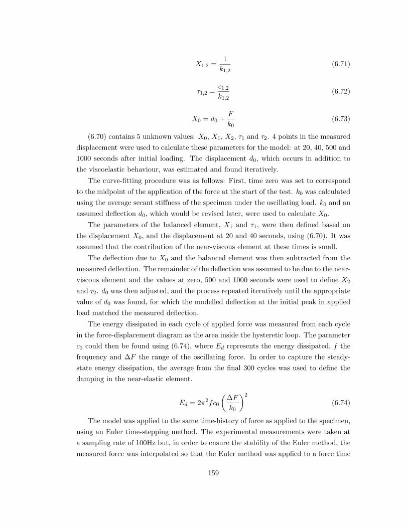
X1,2 =1
k1,2(6.71)
τ1,2 =c1,2k1,2
(6.72)
X0 = d0 +F
k0(6.73)
(6.70) contains 5 unknown values: X0, X1, X2, τ1 and τ2. 4 points in the measured
displacement were used to calculate these parameters for the model: at 20, 40, 500 and
1000 seconds after initial loading. The displacement d0, which occurs in addition to
the viscoelastic behaviour, was estimated and found iteratively.
The curve-fitting procedure was as follows: First, time zero was set to correspond
to the midpoint of the application of the force at the start of the test. k0 was calculated
using the average secant stiffness of the specimen under the oscillating load. k0 and an
assumed deflection d0, which would be revised later, were used to calculate X0.
The parameters of the balanced element, X1 and τ1, were then defined based on
the displacement X0, and the displacement at 20 and 40 seconds, using (6.70). It was
assumed that the contribution of the near-viscous element at these times is small.
The deflection due to X0 and the balanced element was then subtracted from the
measured deflection. The remainder of the deflection was assumed to be due to the near-
viscous element and the values at zero, 500 and 1000 seconds were used to define X2
and τ2. d0 was then adjusted, and the process repeated iteratively until the appropriate
value of d0 was found, for which the modelled deflection at the initial peak in applied
load matched the measured deflection.
The energy dissipated in each cycle of applied force was measured from each cycle
in the force-displacement diagram as the area inside the hysteretic loop. The parameter
c0 could then be found using (6.74), where Ed represents the energy dissipated, f the
frequency and ∆F the range of the oscillating force. In order to capture the steady-
state energy dissipation, the average from the final 300 cycles was used to define the
damping in the near-elastic element.
Ed = 2π2fc0
(∆F
k0
)2
(6.74)
The model was applied to the same time-history of force as applied to the specimen,
using an Euler time-stepping method. The experimental measurements were taken at
a sampling rate of 100Hz but, in order to ensure the stability of the Euler method, the
measured force was interpolated so that the Euler method was applied to a force time
159

10 20 30 40
Dis
pla
ce
me
nt(
mm
)
990 1000 1010 1020500 510 520 530 540Time (s)
ModelMeasured
c = 0.20350
k = 78.970
c = 34131
k = 316.01
c = 2051002
k = 447.32
d = 0.2500
0.25
0.3
0.35
0.4
Figure 6-24: Comparison of displacement time-history between measured response andfinal 7-element rheological model
history with 1000 samples per second.
6.6.1.2 Model accuracy
The measured and modelled values of displacement are plotted against time in Figure
6-24. It can be seen that the modelled response closely follows the response of the
specimen, the largest error being during the first 5 to 10 cycles of load. The near-
elastic element gives the correct amplitude of displacement due to the oscillating load
throughout the test, and the balanced and near-viscous elements follow the creep over
the 1000 second duration of the test. In a similar way that, as described in Section
6.6.1.1, the discrepancy between measured and modelled displacement in the first half
of the test was reduced by the addition of another viscoelastic element with shorter
time constant, the discrepancy in the first 5 to 10 cycles could be reduced by addition
of a further viscoelastic element with an even shorter time constant. It is considered,
however, that the current model, consisting of three Kelvin-Voigt elements, gives a
sufficiently accurate representation for the purpose of the comparisons made between
specimens in Section 6.6.2.
Figure 6-25 shows the 15th, 500th and 1000th cycles of applied force, plotted against
displacement. It is shown that the rheological model captures the creep between each
cycle, shown by the movement of the cycles from left to right. Also captured is the
transient contribution that creep makes to energy dissipation, shown by the higher
energy dissipation in the 15th cycle. The energy dissipation is given by the area inside
the hysteretic loops, and noted as Ed in Figure 6-25. The steady-state energy dissipa-
tion, represented by the damping in the near-elastic element of the rheological model,
is thought to result from both a consistent hysteresis in the timber, and the friction
between the dowel and the timber.
160

Loop 1 MeasuredE
d= 0.00081J
Loop 2 MeasuredE
d= 0.00047J
Loop 3 MeasuredE
d= 0.00040J
Loop 1 ModelledE
d= 0.00083J
Loop 2 ModelledE
d= 0.00046J
Loop 3 ModelledE
d= 0.00047J
Displacement (mm)F
orc
e (
kN
)
1 2 3
8
7.5
7
0.36 0.37 0.38 0.39
Figure 6-25: The 15th, 500th and 1000th force-displacement cycles - Ed represents theenergy dissipated in each cycle
One of the simplifications inherent in this model is that the procedure used to fit
the model to the experimental results considers only the time under the mean load,
and not the number of cycles of load applied. It is considered that this approach is
suitable because of the relatively small magnitude of the oscillating component of the
load compared with its mean. A good representation of the overall behaviour has been
achieved by considering the viscoelastic response to the mean load, and superimposing
upon that the response to the oscillating load as a separate lightly-damped element.
The small amplitude and high frequency of the oscillating component means that the
heavily-damped parts of the model, the balanced and near-viscous elements, do not have
a significant response at the frequency of the oscillating load, and can be considered as
responding to a constant load at the mean value.
The fact that the heavily-damped parts of the model are derived based only on the
mean of the oscillating load does not mean they do not affect the oscillating response,
however, and it is shown, in Figures 6-24 and 6-25, that the model reflects the measured
transient effects on displacement and damping. It is noted that this approach may not
be suitable for larger amplitudes of oscillating load, but it is considered that this model,
and the approach used to fit it to the experimental results, captures several important
features of the behaviour of timber in embedment due to the small-amplitude vibration
which is regularly experienced by structures in service.
161

6.6.2 Comparison of specimens
For each specimen, three equivalent stiffnesses are presented, based on the parameters
of the fitted rheological model. They are illustrated in Figure 6-26. The first, which
will be referred to as the dynamic stiffness kd, is equal to k0, the stiffness of the near-
elastic element. This is the stiffness which would determine the natural frequency of
a structure containing this type of connection, oscillating in the range used in these
tests. The second equivalent stiffness is the series combination of k0, k1 and k2, as
in (6.75), and represents the stiffness under a static load, once all the viscoelastic
elements have relaxed. This is called the viscoelastic stiffness kv. It only includes the
viscoelastic components which are apparent over the 1000 second duration of these
tests, so it represents the stiffness appropriate to calculate the relative displacement
due to a short-term static load, such as crowd, wind or vehicle loading on a structure.
kv =
(1
k0+
1
k1+
1
k2
)−1(6.75)
The third equivalent stiffness is called the total stiffness kt, and includes the vis-
coelastic stiffness combined with the effect of d0. This stiffness would be appropriate to
calculate the total deformation of the connection from initial loading due to, for exam-
ple, the self-weight and imposed loads on a structure. It does not allow for longer-term
creep effects which were not apparent in the 1000 second test. The total equivalent
stiffness is given by (6.76).
kt =
(1
kv+
d0Fav
)−1(6.76)
Figure 6-27 shows the equivalent stiffnesses plotted for each specimen tested. The
three equivalent stiffnesses are substantially different in each specimen. For example,
over the complete set of tests the dynamic stiffness is, on average, 3.8 times higher than
the total stiffness. This difference suggests that each type of behaviour would be best
represented in elastic analysis by a different value of stiffness, and shows the importance
of considering the nature of the loading in determining an equivalent stiffness for a
connection.
Table 6.5 shows the mean of the stiffness for each of the three repetitions of each
type of specimen and orientation. The stiffness is also expressed as the foundation
modulus K, given by (6.77), where w is the length of the specimen along the dowel
axis, and d is the dowel diameter.
K =k
wd(6.77)
162

0 0.1 0.2 0.3 0.40
2
4
6
8
Displacement (mm)
Forc
e (
kN
)
1
1
kv
kd
kt
1
Mean of oscillating force
k - dynamic stiffnessd
k - viscoelastic stiffnessv
k - total stiffnesst
Figure 6-26: The three equivalent stiffnesses used to describe the response of eachspecimen - the 1000 cycles at 1Hz have been omitted for clarity
Dynamic Viscoelastic Total0
20
40
60
Stiffness (
kN
/mm
)
Norway spruce screw parallel
Dynamic Viscoelastic Total0
2
4
6
8
10
12
Stif
fness (
kN
/mm
)
Norway spruce screw perpendicular
0
20
40
60
Stiffness (
kN
/mm
)
Norway spruce 12mm dowel parallel
2
4
6
8
10
12
Stiffn
ess (
kN
/mm
)
Norway spruce 12mm dowel perpendicular
Dynamic Viscoelastic Total Dynamic Viscoelastic Total
0
40
80
120
Stiffness (
kN
/mm
)
Douglas fir 20mm dowel parallel
5
10
15
20
25
Stiffness (
kN
/mm
)Douglas fir 20mm dowel perpendicular
Dynamic Viscoelastic Total Dynamic Viscoelastic Total0
0
Figure 6-27: Equivalent stiffness calculated using fitted rheological model parameters
163

The ratio of the viscoelastic stiffness to the dynamic stiffness is consistent between
the dowel specimens. This suggests that it may be possible to develop an empirical
relationship between these equivalent static stiffnesses, on the basis of further tests,
which could be used in design.
The total stiffness depends on the contribution from d0, which is thought to depend
on errors in construction such as oversize of the hole due to movement of the drill
bit, and on the quality of the interface between dowel or screw and timber. These
parameters are difficult to control, and can be expected to vary between individual
specimens. The variation in total stiffness was, therefore, expected.
164

Tab
le6.
5:M
ean
stiff
nes
san
dfo
un
dat
ion
mod
ulu
sfr
omrh
eolo
gica
lm
od
el
Mea
nd
yn
amic
Mea
nd
yn
amic
stiff
nes
sfo
un
dat
ion
mod
ulu
sV
isco
elas
tic
Tota
l
kd
Kd
kv
orKv
kt
orKt
Sp
ecim
enO
rien
tati
onkN
/mm
kN
/mm
2/m
m%
%
Dou
glas
fir
and
20m
md
owel
Par
alle
l10
0.30
83.5
875
%29%
Per
pen
dic
ula
r19
.48
16.2
372
%35%
Nor
way
spru
cean
d12
mm
dow
elP
aral
lel
53.1
311
0.68
74%
17%
Per
pen
dic
ula
r9.
5319
.85
74%
45%
Nor
way
spru
cean
dsc
rew
Par
alle
l43
.30
144.
3350
%12%
Per
pen
dic
ula
r10
.15
33.8
468
%22%
165

6.6.3 Initial plastic deformation
Some further discussion of the nature of the displacement d0 is considered appropriate,
since it represents a large proportion of the total deformation of the connection, and
appears to be far from linear-elastic.
If the dowel and the half-hole in the timber member do not have exactly the same
diameter, then the dowel will initially make contact with the timber along a single line
along its length. Any unevenness in the surface of the timber will mean that the line
is split into a series of shorter lines or points. As a force is applied to the dowel, the
pressure on this, initially very small, bearing area will be very high. It appears that this
initial high pressure is sufficient to cause deformation of the timber in small volumes
around the dowel, enough that the force is spread over a larger area and the pressure
reduced.
The result is that a significant part of the initial deformation of the dowel under first
loading is made up of the deformation which accommodates these stress concentrations,
which may be plastic in parts of the timber, and elastic in others. Under subsequent
dynamic loading, especially when the force remains above the level at which all these
imperfections are crushed, the imperfections have little effect on the stiffness of the
specimen. It is believed that this behaviour results in the deflection d0 in the model,
which was incorporated so that the viscoelastic model could be fitted to the rest of the
response.
On the basis of this explanation, the deformation d0 would be expected to depend
on the magnitude of the applied force, but would be expected to tend toward some
value, at which all of the imperfections in the contact surface were taken up.
The magnitude of the initial plastic deformation varies widely between the speci-
mens tested, which is consistent with the hypothesis that it is caused by unevenness in
the contact surface between the dowel and the timber and lack of fit between the dowel
and the hole. Both of these parameters depend on the accuracy of the manufacturing
process.
6.7 Summary
Models have been developed as part of this study to predict the elastic component of
the embedment of a dowel into the timber surrounding it, based on an elastic stress
function, and to use that information in predicting the stiffness exhibited by a single
connector. The mathematical model which takes into account the orthotropy of the
timber and the frictional interaction between dowel and timber has been simplified to
form a method suitable for hand calculation.
166

On the basis of this model, the energy dissipation by friction around the dowel
in embedment was calculated. It was shown that this energy dissipation could be
used to make a prediction of the damping ratio in both the embedment and single-
dowel connection tests. The predicted damping ratio appeared to represent a reliable
minimum damping, which was exceeded by most of the tests. The measured difference
in damping between parallel- and perpendicular-to-grain tests also appeared to be
reflected in the theoretical predictions.
It was recognized that the elastic model was only suitable for predicting the steady-
state secant stiffness under one-sided vibration where the cyclic load remains well above
zero. The discussion and analysis in Chapter 4 showed that this is a common form of
loading in in-service vibration, but a model was sought to quantify the relationship
between this elastic stiffness and the stiffness exhibited under other forms of loading.
For that purpose, a viscoelastic model was used, which enabled a comparison of the
stiffness under initial loading, that due to a change in static load, and the cyclic stiffness
which can be predicted by the stress-function model.
167

168

Chapter 7
Connection and Frame Testing
and Analysis
The experimental results in Chapter 5, and the results of the analysis in Chapter 6 have
provided information on the way the basic component of the dowel-type connection
behaves. Those results indicate various characteristics of the behaviour of individual
connectors, which can be expected to affect the behaviour of a complete connection or
structure. The testing and analysis described in this chapter was designed in order to
investigate how those characteristics influence the response of a complete structure to
in-service dynamic loading.
7.1 Materials and methods
Two structures were tested, designed to illustrate the behaviour of connections as part
of a complete structure. They were:
• a cantilever beam, supported by a moment connection to the laboratory strong
wall with mass imposed by steel blocks at its end; and
• a portal frame with moment connections at each node supported by moment
connections on the strong wall with mass imposed by steel blocks at one of the
nodes away from the wall.
The portal frame was thus rotated from its normal configuration in a structure,
which allowed the self-weight and additional mass to apply a load parallel to the line
of the wall. The setup for each test is shown schematically in Figure 7-1.
The purpose of the cantilever and frame tests was to observe the effect of the
behaviour of the elements of connections investigated experimentally in Chapter 5 and
169

Shaker - holding-down bracket omittedfor clarity
Steel blocks30kg each
Steel plates fixedto strong wall
Dowelled connections withcentral steel flitch plates
Horizontal beams 200 deepby 185 wide by 1650mm long
Vertical beam 200 deepby 185 wide by 1800mm long
Cantilever beam200 wide by 200 deepby 1800mm long
Figure 7-1: Schematic test setup for modal analysis of cantilever and frame structures
modelled in Chapter 6 on the behaviour of a complete connection or structure. The
following characteristics were noted in those embedment and single-dowel connection
tests, which were expected to influence the behaviour of the complete connection and
frame:
• a variation of stiffness with amplitude of applied force due to non-linear force-
displacement response at low load;
• a variation of energy dissipation with amplitude of applied force;
• a transient reduction in energy dissipation in the initial cycles of applied load,
with energy dissipation tending to become constant after sufficient time; and
• a transient increase in stiffness, for tests under load control, in the initial cycles
of applied load, with stiffness tending to become constant after many cycles of
load.
The amplitude of the applied load was varied to observe the effect on stiffness and
energy dissipation. The tests were designed to measure the steady-state stiffness and
damping at each amplitude of applied load, the transient effects being eliminated by
applying a static load for a period before the test, and restarting the tests if any signif-
icant change in the modal properties or displacement was noted during the application
of the oscillating load.
7.1.1 Frames
The size of the frame specimens meant that they could not be loaded by a servo-
hydraulic loading machine so, in contrast to the embedment and single-dowel connec-
tion tests described in Chapter 5, their dynamic properties were measured using modal
170

Shaker
Connectionto wall
Prop
Figure 7-2: Frame specimens during testing
analysis. The structures were excited using an electrodynamic shaker and an instru-
mented hammer. As a result, the frequency of the oscillating forces in the connections
was now determined by the natural frequency of the structure, and the amplitude by
the resonant response of the structure to the applied force. This meant that the oscil-
lating force on the connection was not directly controlled, but could be calculated after
the tests.
Each frame was constructed from Norway spruce glued-laminated timber beams
supplied by Lilleheden. The beams used in the frame tests were 185mm by 200mm,
made up of five 40mm laminates and graded GL28h according to BS EN 1194 (BSI;
1999). The beams were used as delivered, which meant that there were examples of
knots being present near the holes through which the dowels passed. In Figure 7-2,
both frames are shown side by side. The nearer one, Frame B, was being tested, so
the shaker and imposed mass can be seen fixed to that frame, while frame A was
temporarily propped.
7.1.2 Cantilever beams
Similarly, the complete moment connections were tested by modal analysis of forced
vibration. In this case, only the electrodynamic shaker was used to excite the structure.
For the cantilever tests, two geometries of moment connection were tested, each fixed
to a steel plate inserted into a slot at the end of the beam with 12mm steel dowels.
The steel plate was welded to a bracket fixed to the laboratory strong wall. Figure 7-3
shows the geometry of the connection, along with reference numbers for each hole and
171

Steel plate boltedto wall
Glued laminated timber beam
1 2
3 4
5 6
Figure 7-3: Geometry of connections for cantilever beam test and numbering of holes
Table 7.1: Cantilever connection test specimens - see Figure 7-3 for dowel locations
Label No. of dowels Dowel locations Applied mass
A6 6 1 to 6 67kgA2a 2 1 and 5 37kgA2b 2 2 and 6 37kgB6 6 1 to 6 67kgB2a 2 1 and 5 37kgB2b 2 2 and 6 37kg
Figure 7-4 shows the connection and the support from the strong wall.
Two-dowel and six-dowel connections were tested. The dowel arrangement is shown
in Table 7.1. The two-dowel connection was used since it represented the simplest form
of moment connection. The six-dowel connections were tested to represent a more
realistic structural connection, and to reflect the connections used in the frame test.
All the tests were carried out on the same glued-laminated timber beam, of 1.8m total
length. By making connections in either end of the beam, there could be two repetitions
of the tests with six-dowel connections, and four repetitions of the tests with two-dowel
connections. One end of the beam was labelled A and one end B so, for example,
specimen A2a was a test on a two-dowel connection at end A of the beam.
The applied mass was chosen to result in a static load in the connection of approxi-
mately 20% of the predicted yield load for the six-dowel connection, and approximately
40% for the two-dowel connection.
The beam used for the cantilever tests was made from glued-laminated timber
supplied by Lilleheden, graded GL28h according to BS EN 1194 (BSI; 1999). The cross-
section was 200mm by 200mm square, made up of six 33.3mm laminates of Norway
172

Steel platebolted to wall
Dowelledconnection toplate
Figure 7-4: Support for cantilever beam tests showing the six-dowel connection
spruce.
7.1.3 Excitation of structures
Three separate methods were used to dynamically excite each structure, each requiring
a different analysis method. All were forced vibration tests, exciting the structure at
a single point. To preserve the simplicity of analysis in both cases, the excitation was
applied at the same point as the imposed mass: at the end of the cantilever and at the
right angle of the frame. This also meant that the mass of the shaker, significant at
37kg, could form part of the imposed mass. The excitation methods were:
• a slow sine sweep, in which a sinusoidal force, gradually increasing in frequency,
was applied by the shaker and the rate of increase of frequency was sufficiently
slow that the steady-state response at each frequency had time to develop;
• a pseudo-random excitation, in which a signal containing a known range of fre-
quency components with random phase was generated and used to drive the
shaker; and
• an impulse, applied by an instrumented hammer, was applied at the same point
at which the shaker was placed.
Even though the shaker was not used in the impulse tests, it remained in place to
maintain the same distribution of mass in each test. The shaker is shown mounted on
a frame specimen in Figure 7-5.
173

Accelerometer
Shaker
Imposed mass
Movingarmature
Figure 7-5: Detail of frame test, showing the shaker mounted on the structure, themass imposed by steel blocks and one of the accelerometers
Before dynamic testing, the structure was assembled, instrumented and propped
at the point where the mass was to be placed. The prop was set at a height that
made the horizontal members level, as measured with a spirit level. The prop was then
removed, and the displacement monitored for a period of 16 hours to allow the transient
processes to occur: looseness in the connections to be taken up; surface irregularities
at the dowel-timber interface to crush as far as possible; and the initial creep in the
connections to occur. The dynamic tests were then carried out, the slow sine sweep
and pseudo-random excitation applied at a range of amplitudes.
7.1.3.1 Measurement of input force
The force applied by the instrumented hammer was measured by a high-frequency load
cell at its tip. The shaker applied a force to the structure through the inertia of an
armature which moved along a single axis as it was driven by an inductive coil. Since
the shaker was placed on the structure and otherwise unsupported, the variable force
applied to the structure was generated by the inertia of the moving armature, and so
was proportional to its acceleration. That acceleration was therefore measured and
used to calculate the variable applied force.
The relationship between the measured acceleration of the armature and the force
applied to the supporting structure was calibrated using a load cell. The shaker was
mounted on the load cell, and the armature caused to oscillate at a frequency of 8Hz,
representative of the natural frequency of the cantilever and frame structures. The
174

0 0.2 0.4 0.6 0.8 1-4
-2
0
2
4
Time (s)
Accele
ration (
g)
0 0.2 0.4 0.6 0.8 1-0.1
-0.05
0
0.05
0.1
Time (s)
Forc
e (
kN
)
0 0.2 0.4 0.6 0.8 10
0.01
0.02
0.03
0.04
0.05
Time (s)
Ratio
0 0.2 0.4 0.6 0.8 1-2
-1
0
1
2
Time (s)
Accele
ration (
g)
0 0.2 0.4 0.6 0.8 1-0.04
-0.02
0
0.02
0.04
Time (s)
Forc
e (
kN
)
0 0.2 0.4 0.6 0.8 10
0.01
0.02
0.03
0.04
0.05
Time (s)
Ratio
Figure 7-6: Evaluation of the constant of proportionality between the acceleration ofthe shaker armature, and the inertia force applied to the supporting structure
measured plots of force and acceleration were then compared and used to estimate the
constant of proportionality between the two.
The analogue to digital conversion for the load cell did not have sufficient discrete
points in the amplitude of the applied force for an accurate representation of the load
profile, but the representation was considered sufficiently accurate that, averaged over
200 cycles, a representative value of the ratio of acceleration to force could be estimated.
When the force and acceleration were close to zero, the result was sensitive to errors
in either, so the average was calculated using only values greater than 9.81m/s2, or
1g. To verify proportionality, the ratio between the two readings was evaluated at two
amplitudes of acceleration. The results are shown in Figure 7-6.
The structures were instrumented so that both displacement and acceleration of
various points of the structure could be measured. The location of sensors is shown in
175

Figures 7-11 and 7-16, later in this chapter. Given the time history of the force applied
to the structure, either from the acceleration of the shaker armature or the instrumented
hammer, and the time history of displacement and acceleration from these sensors, two
transfer functions could be directly calculated: the receptance and the accelerance. The
former is the relationship between displacement and applied force over the frequency
range, and the latter the relationship between acceleration and applied force. The
component of receptance Hx(ω) at each frequency can be transformed into accelerance
Ha(ω), and vice versa, by the relationship Ha(ω) = −ω2Hx(ω), so the two could be
compared to verify the accuracy of the measurements.
7.2 Analysis
7.2.1 Modal analysis
The input force spectrum could therefore be obtained from the measured acceleration
of the shaker armature, and the response from the accelerometers and displacement
transducers around the structure. The concentration of mass in each structure, and
the fact that the excitation was applied along a single axis, meant that the response of
each was dominated by a single mode of vibration. The purpose of the modal analysis
was to identify the natural frequency and modal damping, as well as the presence of
any nonlinearity, in that single mode.
For the pseudo-random tests, the precision of the measured transfer function de-
pended on the sampling rate and the length of the measured time-histories of dis-
placement and force. Pilot tests showed that a test of 100s duration sampled at 200Hz
provided a sufficiently well-defined transfer function, and these were used on the pseudo-
random vibration tests on the cantilever joints and frames.
In the slow sine sweep tests, a sampling rate of 200Hz was again used. The duration
of the test had to be chosen so that the rate of sweep was slow enough for the full
resonant response to develop at each frequency of applied force.
The amount of time for the full resonant response to develop depends on the natural
frequency and damping in the system, since it represents the time at which the energy
dissipated by the system in one cycle equals the energy put into the system by the
oscillating force in that cycle. In a system with high damping, this condition will be
more quickly met compared with a system with low damping, where the amplitude
must increase further before the energy balance is satisfied. For a system with a given
damping, the balance of input and dissipated energy is achieved over a given number
of cycles. For a higher-frequency mode, therefore, the balance of input and dissipated
energy is achieved in a shorter time than in a lower-frequency mode.
176

The natural frequency and damping of the mode in consideration therefore influence
the time taken for the system to reach its steady-state response at resonance, and so
influence the rate at which the frequency should be increased in a slow sine sweep
test. ISO 7626 (ISO; 1990) gives guidance on the appropriate rate of sweep for modal
analysis for a model with a given natural frequency and damping. The equation given
in that code, adjusted to use the notation used in this study, where f is frequency in
Hertz, fn is the natural frequency of the mode in question, γ is the equivalent viscous
damping ratio and t is time, is given in (7.1).(df
dt
)max
= 216f2nγ2 (7.1)
The natural frequency of the system was estimated based on pilot tests and a
conservatively low estimate of damping, 1.5%, was used to determine the sweep rate
for use in the tests.
Once the tests had been conducted, the transfer function, either accelerance or re-
ceptance, was plotted from the measured acceleration or displacement. For the slow
sine sweep excitation, the accelerance could be calculated by converting the time histo-
ries of force and acceleration to their frequency-domain spectra using a discrete Fourier
transform, MATLAB’s built-in fft function, resulting in a complex number at each fre-
quency representing magnitude and phase, and then dividing acceleration by force at
each frequency. Using the measured displacement, the receptance could be calculated
in a similar way.
For the pseudo-random excitation, even though the pseudo-random signal is gener-
ated to contain a range of frequencies, the Fourier transform of the input force is not
constant over that range of frequencies, but varies sharply. As a result, slight errors in
the measured magnitude and frequency of displacement or acceleration lead to large er-
rors in the transfer function if it is calculated simply by dividing the Fourier transform
of the output by that of the input. For the case of pseudo-random excitation, a more
accurate measurement of the accelerance Ha can be made by using the relationship be-
tween it, the autocorrelation of the input force Pff and the cross correlation between
force and acceleration Pfa (Ewins; 1986), as given by (7.2). A similar relationship
exists for receptance.
Ha =PfaPff
(7.2)
For both forms of excitation, the natural frequency and modal damping were ini-
tially investigated by the circle fit method. The brief investigation into the frequency
dependence of energy dissipation described in Section 5.3.2 concluded that the hys-
177

teretic damping model was the most appropriate for the observed embedment be-
haviour. The circle fit method used here therefore uses the fact that the receptance
of a single-degree-of-freedom system with hysteretic damping, plotted on the complex
plane, forms a circle, as shown in Figure 7-7. The value of the receptance moves around
the circle as the frequency is increased, and it can then be shown (Ewins; 1986) that
rate of sweep of the receptance function around the circle is a maximum at resonance.
The resonant frequency ωr can therefore be determined using a finite difference method
to locate its value between the measured points.
The finite difference method was applied by first calculating the rate of sweep dθ/dω
for each pair of measured points on the receptance plot. Call this rate of sweep θ′. The
maximum rate of sweep could then be seen to lie between two points, θ2 and θ3. The
location of the maximum rate between those two points could then be estimated using
(7.3) to (7.6), a finite difference method which can be derived from the Taylor series,
which uses the circular frequency and phase angle at four points, ω1,2,3,4.
Where θ′ has its maximum, θ′′ will be equal to zero. The second derivatives θ′′2and θ′′3 are therefore estimated using (7.3) to (7.5). The frequency at which the max-
imum rate of sweep occurs, ωr, equal to the natural frequency, is then estimated by
interpolation between ω2 and ω3, as in (7.6).
h = ω3 − ω2 (7.3)
θ′′2 ≈θ3 + θ1 − 2θ2
h2(7.4)
θ′′3 ≈θ4 + θ2 − 2θ3
h2(7.5)
ωr ≈ ω2 + hθ′′2
θ′′2 − θ′′3(7.6)
The circle fit can also be used to estimate damping, since the equivalent viscous
damping γ is given by (7.7), where ωa and ωb are arbitrary frequencies either side of ωr,
and θa and θb are their respective angles measured around the circle from ωr. Since any
pair of data can be used to estimate the damping, it is common to use every possible
pair of points in the vicinity of a resonant frequency to calculate the damping, and
so to construct a matrix of damping estimates. By plotting this matrix of damping
estimates, the accuracy of the measurements, the accuracy of the estimate of ωr and
the linearity of the system being measured can be inferred. This is discussed further
later in this section.
178

γ =ω2a − ω2
b
2ωr
(ωa tan θa
2 + ωb tan θb2
) (7.7)
Using the accelerance calculated from the test results,the circle-fit method was used
to estimate damping and natural frequency as follows:
• the accelerance spectrum was converted to the equivalent receptance spectrum
by multiplying by −ω2, equivalent to integration twice in the time domain;
• a set of receptance values in the vicinity of the resonant peak was selected and
plotted on the complex plane;
• a circle was fitted to the points on the complex plane (Bucher; 1991), and the point
on the circle corresponding to resonance was estimated using a finite difference
method;
• the damping was estimated using (7.7), with each frequency used to create the
circle paired with every other frequency used to create the circle; and
• the resulting matrix of damping estimates was plotted.
A flat surface in the plot of damping estimates, corresponding to equal estimates
of damping using each pair of frequencies, would indicate a system behaving linearly,
measured with sufficient accuracy and a correct estimate of the natural frequency. The
MATLAB script written to perform the circle fit method included the option to make
fine alterations to the natural frequency estimate to look for a more consistent set of
damping estimates.
Figure 7-7 shows the steps in the circle fit method for the response of connection
A to pseudo-random excitation. It can be seen that the set of damping estimates
forms an approximately flat surface, albeit with some systematic variation due to the
nonlinearity in the system, the imperfect fit of the circle and any inaccuracy in the
damping estimate. The average of the set of damping estimates is taken to be the
measured damping.
If the system behaves in a more nonlinear way, then it is not possible to achieve a
consistent set of damping estimates. This was the case for several of the tests carried
out as part of this study, and so, for those tests, another approach was developed to
estimate the natural frequency and damping, based on a theory of nonlinear vibration.
179

9
10
11
7.5
8
8.5
90
1
2
3
Frequencyabove f (Hz)r
Frequencybelow f (Hz)r
Dam
pin
g r
atio
(%)
γ
7.5 8 8.5 9 9.5 10 10.5 11-7
-6
-5
-4
-3
-2
-1
0
Frequency (Hz)
θ
θn= -3.19
-2 -1 0 1 2 3 x10⁻⁵
-3
-2
-1
0
x 10-5 Nyquist Plot with Circle Fit
Real(H (f))x
Imag(H
(f))
x
θ
6 7 8 9 10 11 12 130
2
4
6
8x10
-5Receptance Spectrum
Frequency (Hz)
|H(f
)|x
ReceptanceRange of pointsused in circle fit
f = 9.28Hzn
= 2.21γ
Figure 7-7: Estimates of damping γ and natural frequency fn using the circle-fit methodfor connection A under pseudo-random excitation
180

7.2.2 Nonlinear vibration
It has been seen in the experimental results in Chapter 5 that, for an oscillating force
with R=1.2, the force-displacement plot for embedment or for a single-dowel connection
appears close to linear. As the amplitude of oscillating force is increased so that R=10,
the force-displacement response is noticeably non-linear, and the nonlinearity led to a
reduction in the secant stiffness.
In the forced-vibration tests on connections and frames described in this chapter,
the applied force on the connection cannot be directly measured, so force-displacement
plots cannot be drawn. The reduction in stiffness can be observed as a reduction in
natural frequency, but the nonlinearity also has the effect of changing the measured
accelerance of the system under harmonic excitation.
The effect of the nonlinearity in the system can be described using a method devel-
oped by Duffing (1918). Duffing carried out an extensive study into the equation given
in (7.8), which describes the oscillation of a system with undamped natural frequency
ωn and viscous damping ratio γ, under a harmonic force f . The linear restoring force
in Duffing’s oscillator is generated by the natural frequency squared ω2n, equal to the
linear stiffness per unit mass k/m, multiplied by the displacement x. There is also a
component of the restoring force proportional to x3, with constant of proportionality
µ3. This will be referred to as the cubic stiffness. Duffing’s equation is therefore identi-
cal to the equation of motion for a single degree-of-freedom dynamic system, but with
an additional cubic component in the restoring force.
x+ 2γωnx+ ω2nx+ µ3x
3 = f (7.8)
The cubic stiffness term represents a system whose secant stiffness changes with
amplitude. A positive value of µ3 represents a ‘hardening’ system, whose stiffness
increases with amplitude, and a negative value represents a ‘softening’ system whose
stiffness decreases.
Duffing (1918) solved this equation using the method of successive approxima-
tion. Given harmonic excitation, it was assumed that the response would also be
harmonic, though not necessarily in the same phase. The forcing function is given by
f = F cos(ωt+ φ), and the response has the form x = X cos(ωt).
The first approximation for x was therefore taken as in (7.9), with f rewritten as
in (7.10). Substituting this into the equation of motion and rearranging gives (7.11).
x0 = X cos(ωt) (7.9)
181

f = F1 cos(ωt) + F2sin(ωt) (7.10)
x0 = 2γωnωX sin(ωt)− ω2nX cos(ωt)− µ3X3 cos3(ωt) + F1 cos(ωt) + F2 sin(ωt)
= 2γωnωX sin(ωt)− ω2nX cos(ωt)− µ3X3
(3
4cos(ωt) +
1
4cos(3ωt)
)+ F1 cos(ωt) + F2 sin(ωt)
(7.11)
In the method of successive approximation, (7.11) is integrated to give a second
approximation, x1, given in (7.12). Assume the steady state response to the forcing
function, so that the constants of integration are zero.
x1 =
∫∫ (F1 − ω2
nX − µ3X3 3
4
)cos(ωt)− µ3X3 1
4cos(3ωt)
+ (F2 + 2γωnωX) sin(ωt)dt
= −(F1 − ω2
nX − µ3X3 3
4
)1
ω2cos(ωt) + µ3X
3 1
36ω2cos(3ωt)
− F2 + 2γωnωX
ω2sin(ωt)
(7.12)
The cos(3ωt) term arises because of the cubic stiffness, and further iterations would
suggest components of the response at higher amplitudes with smaller magnitudes.
Based in this first approximation, though, (7.12) suggests a response dominated by the
cos(ωt) term, which justifies the assumed form of the response given in (7.9). Duffing
(1918) proposed that if both x0 and x1 are approximations of the true response of the
system, then the coefficients of cos(ωt) and sin(ωt) in each should be equal, so that
an approximate solution to the equation of motion is given by equating the two, as in
(7.13) and (7.14).
X =ω2n
ω2X +
3
4ω2µ3X
3 − F1
ω2(7.13)
0 = F2 + 2γωnωX (7.14)
The magnitude of the forcing function F is given by F 2 = F 21 + F 2
2 , so using
(7.13) and (7.14), (7.15) can be written. For a given magnitude of the forcing function,
damping and natural frequency, (7.15) becomes a cubic equation in X2, which can be
182

-10 -5 0 5 10-50
0
50
Forc
e (
N)
9 9.5 10 10.5 111
2
3
4
5
6
7
Recepta
nce (
mm
/N)
Linear
Hardening
Softening
Displacement (mm) Frequency (Hz)
Figure 7-8: Receptance plots for Duffing oscillators with a linear natural frequency of10Hz, mass of 1kg and a viscous damping ratio of 2%, under an oscillating load withmagnitude 1N
solved for a range of frequencies to plot the transfer function for the theoretical system.
F 2 =
(3
4µ3X
3 + (ω2n − ω2)X
)2
+ (2γωnωX)2 (7.15)
Figure 7-8 shows the receptance plots for linear, hardening and softening systems,
calculated using (7.15). In each case, all the parameters are kept constant except
µ3, which was 4 × 10⁶N/m3 for the hardening system and −4 × 10⁶N/m3 for the
softening system. The effect of the cubic stiffness component on the receptance can be
seen. In the softening system, the frequency for the peak response is lower than the
linear system, and the magnitude of that peak response higher. The hardening system
displays the opposite tendencies.
In the embedment and single-dowel connection tests, the stiffness was observed
to decrease with an increasing amplitude of oscillating load. This corresponds to a
negative value of µ3 in Duffing’s method.
As shown in Figure 7-9, the gradient of the centreline measured in the embedment
tests does not reduce in gradient symmetrically either side of the centre of the oscillating
force, as is modelled by the kx + µ3x3, with negative µ3, in Duffing’s equation. The
behaviour is, in fact, asymmetrical around the centre of oscillation, with the gradient
increasing throughout the upward stroke of the cycle, though at a reducing rate. This
asymmetry can be approximated by introducing an η2x2 term into Duffing’s equation
(7.16).
x+ 2γωnx+ ω2nx+ η2x
2 + µ3x3 = f (7.16)
183

0.16 0.2 0.240
4
8
12
Displacement (mm)
Forc
e (
kN
)
Single cycleCentreline
Figure 7-9: The centreline of the force-displacement diagram for a Douglas fir embed-ment specimen loaded parallel-to-grain to 40% of its predicted yield load with R = 10
The effect of the η2x2 term is to introduce a term in cos(2ωt) into the second
approximation of the displacement, x1, as in (7.17). Thus the response at the natural
frequency is unaffected, but a further harmonic is introduced by the quadratic stiffness
at double the natural frequency.
x1 = −(F1 − ω2
nX − µ3X3 3
4
)1
ω2cos(ωt) + η2X
2 1
8ω2cos(2ωt)
+ µ3X3 1
36ω2cos(3ωt)− F2 + 2γωnωX
ω2sin(ωt)
(7.17)
Ewins (1986) investigated the effect of cubic stiffness behaviour on the use of the
circle-fit method, described in Section 7.2.1, for estimation of natural frequency and
damping by using a signal generator to replicate the response of a system with cu-
bic stiffness. He showed that the linearisation inherent in the analysis technique for
pseudo-random excitation meant that, for that form of excitation, plotting the matrix
of damping estimates still resulted in a flat surface, allowing a damping estimate to
be made. In contrast, plotting the matrix of damping estimates resulting from the
circle fit of a slow sine sweep test showed a systematic variation of damping, so that a
reliable damping estimate could not be made. In this study, therefore, a curve-fitting
approach is used to extract modal properties from the measured accelerance, described
in Section 7.4.1.
7.3 Theoretical prediction
The stress function model for embedment, presented in Chapter 6, along with a beam-
on-elastic-foundation model to allow for the elasticity of the connector, was shown to
184

predict the stiffness of a single-dowel connection under small-amplitude oscillating load.
An increase in amplitude of load resulted in nonlinear behaviour not predicted by the
model.
In the structures tested in this chapter, each connection has multiple connectors,
loaded at varying angles to the grain and the connections form part of a larger struc-
ture. The method was therefore extended to allow for each of these features, by using
conventional approaches from timber engineering.
7.3.1 Dowel groups and angle to grain
The stress function approach developed in Chapter 6 was shown to be suitable for esti-
mation of the stiffness due to a single connector loaded either parallel or perpendicular
to grain. In this study, where the load is applied neither parallel nor perpendicular to
the grain, the calculated stiffness for each case is interpolated using the equation by
Hankinson (1921). As discussed in Section 2.2.5, this equation is considered to be a
sensible choice for an initial estimate of the effect of angle to grain on stiffness, since
it has been widely used to estimate the variation of strength, and has been shown by
Schniewind and Barrett (1972) to apply to creep. The true variation of stiffness with
angle to grain, however, should be a subject for further analytical and experimental
study.
The behaviour of a group of dowels in a moment connection was discussed in Sec-
tion 2.2.3, with particular reference to work by Noguchi and Komatsu (2004), which
suggested that, in order to correctly model an asymmetrical arrangement of dowels in
a moment connection, the force in each dowel cannot simply be assumed to be pro-
portional to its distance from the centre of rotation. Instead, Noguchi and Komatsu
(2004) presented a design method based on Saint-Venant torsion theory. The basis
of Noguchi and Komatsu’s calculation was different to that used in this study, in that
their calculation was based on a single foundation modulus, independent of the distance
of the connector in question from the centre of rotation.
In this study, it has been shown that the dependency of the foundation modulus on
the distance of the dowel from the centre of rotation can be modelled. By incorporating
that dependency according to the stress-function model from Chapter 6, and the effect
of grain orientation on the foundation modulus, the fundamental assertion of Noguchi
and Komatsu’s work, that the force in each dowel is not, in general, proportional to
its distance from the centre of rotation, is considered to be satisfied. The displacement
of each dowel relative to the centre of rotation is assumed to be proportional to its
distance from the centre of rotation, but the difference in foundation modulus, and
therefore in the stiffness of each dowel, ensures that the forces vary. For the purpose
185

0
0.5
1
1.5
2
0 0.5 1 1.5
31,2
4,5
6,7
8,9
10,1112,13
x coordinate (m)
y c
oord
inate
(m
)
Nodes 1 and 13fixed for translationand rotation
Distributed mass on allmembers, concentratedmass at node 3
Figure 7-10: Geometry of the frame and node numbering for the stiffness matrix model
of this study, therefore, the conventional equation for the stiffness Kr of a moment
connection with n connectors given, for example, by Porteous and Kermani (2007), is
modified to allow for the different stiffness in different connectors to give (7.18), where
Kbf is the stiffness for each connector and l the distance of each connector from the
centre of rotation.
Kr =n∑i=1
Kbf,il2i (7.18)
7.3.2 Stiffness matrix models
The dynamic response of the frame was modelled using the stiffness matrix method.
The analysis was therefore purely elastic, but could be used to incorporate the effect of
the rotational and translational movement in the connections. It was considered that
the cyclic stiffness, measured in Chapter 5, of individual dowels under load with R=1.2
could be adequately represented by a lightly-damped linear-elastic model. An elastic
frame with semi-rigid connections was therefore considered appropriate to predict the
stiffness properties of the frame, as long as the amplitude of vibration was sufficiently
small.
A stiffness matrix was generated for the frame using MATLAB. The geometry and
node numbering is shown in Figure 7-10, and the properties of the nodes and the
members or connections between them are given in Table 7.2.
186

Table 7.2: Properties of nodes and members in the stiffness-matrix model for the framestructure
Node Location Connection
1 Fixed to wall6-dowel connection
2 On beam200mm by 185mm timber beam
3 On beam200mm by 185mm timber beam
4 On beam4-dowel connection
5 On plate160mm by 6mm steel plate
6 On plate4-dowel connection
7 On beam200mm by 185mm timber beam
8 On beam4-dowel connection
9 On plate160mm by 6mm steel plate
10 On plate4-dowel connection
11 On beam200mm by 185mm timber beam
12 On beam6-dowel connection
13 Fixed to wall
187
The dowel-type connections are represented by placing two nodes at the same loca-
tion, corresponding to the centroid of the connection, and defining the stiffness between
them based on the linear and rotational stiffness of the connection. The stiffness of
each individual connector was estimated using the complex stress function approach
for a dowel through a complete hole described in Section 6.1.2, and the stiffness of each
complete connection estimated based on each connector resisting a force in proportion
to its distance from the centroid of the connection, thus following the method given by
Porteous and Kermani (2007).
In a complete structure with many connections, not all of them would be expected to
be highly loaded simultaneously under in-service conditions. In this frame, the applied
loads were chosen so that the most loaded connection, the 6-dowel lower connection to
the strong wall, would be subject to a peak load of 20% of its predicted failure load for
vibration with R=1.2. The upper connection to the strong wall is subject to a peak
load of 19% of its predicted failure load in the same condition. The 4-dowel connections
between the timber members, however are only loaded to 10% of their predicted failure
load in that case. This ratio of applied load to capacity is considered to be a reasonable
representation of the loads that a structure would be expected to experience in service.
One of the reasons that it was decided to carry out the stiffness matrix analysis in
MATLAB, rather than with proprietary software for the purpose, was to have control
over the semi-rigid connection stiffness, and to be able to apply translational as well
as rotational stiffness of connections. Another reason was that by using MATLAB, the
stiffness matrix could be accessed and manipulated to obtain more information about
the behaviour of the structure, such as the distribution of stored energy.
The distribution of stored energy can be used to estimate the damping ratio in the
structure. In a similar way that the stiffness in each element is combined to assess
the stiffness of the complete frame, the energy dissipation in the complete frame as it
vibrates consists of a combination of the energy dissipation in each element. The total
energy dissipation is taken to be the sum of the energy dissipation in each element.
The energy dissipation in each element is then related to the damping ratio, which
describes the proportion of the elastic stored energy that is dissipated in each cycle.
In this work, for consistency and to follow the convention most commonly used in
structural dynamics, the equivalent viscous damping ratio has been used throughout.
The equivalent viscous damping ratio γ is given by (7.19), where Ed is the dissipated
energy per cycle and W is the energy continually alternating between the kinetic form,
as the movement of the mass, and the potential form, as the elastic stored energy in
the frame.
188

3D
5A
1640mm
Centroid of dowels to
centreline of shaker
3DTransducer location
D: displacement; A: acceleration
Reference number
4A
Figure 7-11: Transducer and shaker locations on the cantilever joint structure
γ =Ed
2πW(7.19)
Given the damping ratio of an element, therefore, the energy dissipated can only be
calculated if the magnitude of the elastic stored energy, otherwise known as the work
done on the element, is known. Assuming linear-elastic behaviour, the work done on
each part of the system can be readily calculated from the matrices of stiffness, K, and
displacement, X, in the stiffness-matrix analysis of the frame.
W =1
2XTKX (7.20)
7.4 Results and discussion
7.4.1 Cantilever beams
The location of the transducers on the cantilever joint structure and their numbering
system are shown in Figure 7-11. The displacement transducer was used to measure
the deformation under the static load applied for 16 hours before testing, and as a
check for the readings from the accelerometer mounted at location 5 on the steel block.
The accelerometer at location 4 measured the movement of the armature of the shaker
to calculate the input force.
The capacity of the connection was calculated according to Eurocode 5 (BSI; 2009a),
using the density of the timber measured using the weight and volume of the beam. For
the six-dowel connections, the applied static loads resulted in a force per shear plane
of 2.34kN in the highest-loaded connector, which was found to be equivalent to 18% of
the capacity of the connection according to Eurocode 5. The static load applied to the
two-dowel connection was equivalent to 39% of the capacity.
189

0 10000 20000 30000 40000 500000
5
10
15
20
Time (s)
Dis
pla
cem
ent (m
m)
Figure 7-12: Deflection of cantilever beam A under its self weight and an imposed loadof 657N at its end over a 16-hour period
The first part of the test process was to apply a static load to the connection
for a period to eliminate part of the expected transient behaviour. For the six-dowel
connections, the load was applied for 16 hours, and for the two-dowel connections, since
the same dowels had already been subject to the 16-hour loading, 15 minutes. The
dynamic tests were then carried out over an extended period of time after preloading,
which included leaving the static load in place overnight between dynamic tests. The
displacement of connection A6 during 16 hours under the static load of its self-weight,
the weight of the shaker and that of the steel block is shown in Figure 7-12. The
deformation was measured at the tip of the cantilever at location 3 in Figure 7-11.
It can be seen in Figure 7-12 that the immediate deformation forms a large part
of the total deformation of the connection. The bending and shear deformation of the
timber cantilever beam was calculated to represent less than 1mm of deflection at the
tip, and so less than 5% of the total measured deflection. The remainder was due to
the rotation and vertical movement in the connection. The deformation can be seen
to follow a curve indicative of viscoelastic behaviour under constant load, with the
addition of several rapid steps in displacement, of the order of 0.1mm at the tip of
the beam. When one of these steps occurred, there was an audible creak, which was
thought to be a sign of frictional slip.
A possible explanation for these steps in displacement is that, due to the uninten-
tional misalignment of the holes in the timber and the steel plate, the contact force
between the dowel and the steel plate is asymmetrical, with the force transferred at a
point of contact which is not at the apex of the hole in the plate, as shown in Figure
190

Dowel
Timber
Resultant forcedirection on plate
Hole in steel plate
Misalignment ofholes in steel andtimber
Offset contact forcesbetween plateand dowel
Figure 7-13: The affect of misalignment of the hole in the steel flitch plate with thedowel on force transfer
7-13. This position is unstable, in that as the timber deforms, the dowel can move
closer to the apex of the hole, perhaps as a rapid slip as the stress relaxation in the
timber reduces friction forces supporting the asymmetrical load. This behaviour would
be extremely difficult to predict, since it results from inaccuracies in construction, but
with time under load, as creep occurs in the timber, each dowel would be expected to
slip towards the stable state in which the dowel was loaded at the apex of the hole.
After the time under static loading was complete, dynamic loads were applied using
the shaker, which had been attached to the beam forming part of the static load. The
displacement measured at location 3 in Figure 7-11 was observed during each test,
and a further step in displacement was occasionally observed under dynamic load. If
this occurred, it generally had a subsequent effect on the resonant frequency, due to
the change in stiffness, and so the series of dynamic tests was restarted. The results
presented here, therefore, are for a series of tests for which the final static displacement
was not significantly different from the initial resting displacement, and this set of
results is considered to be representative of the steady-state behaviour of the system.
7.4.1.1 Six-dowel connections
First, the analysis of the results of the six-dowel connection tests, on connections A6
and B6, will be presented and discussed, since they were carried out first, and it was
on the basis of these results that the procedures for analysis of nonlinear vibration
were developed. For the slow sine sweep tests, the modal properties were estimated by
curve fitting the receptance for the fundamental mode of vibration using the theoretical
receptance function, from Section 7.2.2, for a system with cubic nonlinearity. The curve
fitting was carried out using the MATLAB function fminsearch to minimize the sum
191

Table 7.3: Modal mass of the fundamental mode of vibration of the cantilever beam,calculated using the circle-fit method on the pseudo-random vibration response of can-tilever B6
Test Root Mean Square Amplitude Estimated Modal Mass(N) (kg)
BN0.5 8.9 78.3BN0.75 13.2 77.1BN1 17.6 82.3
of the square of the difference between the experimental and theoretical curves at each
point.
The curve-fitting procedure allows estimation of the natural frequency, the linear
stiffness component, the cubic stiffness component and the damping in the system.
For the pseudo-random excitation, the same parameters could be identified using the
circle-fit method, described in Section 7.2.1, with the exception of the cubic stiffness
component, since the linearlization inherent in the use of auto- and cross-correlation
functions used to generate the measured receptance function resulted in a symmetrical
receptance plot.
The known variable was the modal mass of the system, calculated by the application
of the circle-fit method to the pseudo-random vibration test results for connection
B6. Since the connections were at either end of the same beam, the modal mass was
expected to be very similar for connection A6. The modal mass calculated from each
of the three pseudo-random vibration tests is given in Table 7.3, and the mean value,
79kg, was used for curve fitting.
The three unknown variables, the damping and the linear and cubic components
of the stiffness, were then obtained by fitting a receptance function for a system with
cubic stiffness to the measured receptance.
The cubic nonlinearity was chosen because of its mathematical convenience, and
because the receptance function for cubic nonlinearity had been defined by Duffing
(1918). The extent to which the stiffness reduced with amplitude was not expected to
be precisely represented by a cubic function, since the use of the cubic function had
no basis in the behaviour of the connection. As a result, the cubic-stiffness receptance
function could not be expected to precisely fit the measured behaviour of the connection
at all amplitudes. It was therefore decided to fit the function to the measured response
in the near vicinity of resonance, since it is in that region that the majority of the
response occurs.
A range of measured points either side of the peak response were used for curve
192

fitting. For consistency across the tests, the range was expressed in terms of the mag-
nitude of the response: the curve fitting encompassed all the points with a magnitude
greater than a given proportion of the peak value. A brief sensitivity analysis was
carried out to investigate the influence of the chosen value of that proportion on the
fitted values of stiffness and damping.
Figure 7-14 shows curves fitted to the measured receptance of a slow sine sweep
test on connection A6 using different ranges of points. It can be seen that if too
wide a range of points is used for the curve fitting, the cubic function does not fit the
behaviour at high and low amplitudes closely enough, resulting in a poor representation
of the measured receptance, as in the lower plot in Figure 7-14, where all receptance
measurements higher than a quarter of the peak value were used to fit the curve.
The values of the parameters estimated by the curve-fitting process are noted in
Figure 7-14. The natural frequency of the linear system is the frequency towards which
the system would be expected to tend as the amplitude of vibration reduces, and the
contribution of the cubic component of stiffness becomes negligible. This corresponds,
according to the interpretation of the models and results in Section 6.4, to the linear
elastic stiffness of the connection in which the contact there is a rigid contact surface
between dowel and timber. The cubic stiffness represents the reduction in stiffness as
the amplitude of vibration increases. The damping ratio was observed to be relatively
insensitive to the change in the points used for curve fitting, which gave confidence
that a reasonable estimate of modal damping could be achieved this way.
The upper plot in Figure 7-14 shows a much closer fit of the measured receptance
over a smaller range of values. It was considered, however, that the middle plot in
Figure 7-14 provided a suitable balance between including sufficient measured data to
accurately represent the measured behaviour in the fitted model, and allowing for the
fact that cubic function could only be expected to represent the real behaviour over
a limited range of amplitudes. In fitting the receptance function for cubic stiffness to
the measured data from the slow sine sweep tests, therefore, a range of data was used
incorporating all the points with a receptance greater than half the peak value.
Figure 7-15 shows the variation of the underlying linear natural frequency, cubic
stiffness and damping as the amplitude of the applied cyclic force increased. The upper
plot in Figure 7-15 shows that the natural frequency of the elastic system is similar
for the two connections. Both show a slight reduction as the excitation amplitude
is increased. This reduction is more prominent in connection A6. In a system with
cubic stiffness, this frequency would be expected to remain constant as the excitation
increased, with the reduction in the frequency of the peak response accounted for by the
cubic component. The fact that the ‘softening’ in the system is not perfectly represented
193

7 7.5 8 8.5 9 9.5 10 10.5 11
1
1.5
2
2.5
3
3.5
4x 10
-5
Frequency (Hz)
Recepta
nce (
m/N
) Linear natural frequency = 8.91HzDamping ratio = 6.3%
Cubic stiffness = -1.1N/mm3
Measured receptanceModelled receptance
Cut off at peak response
divided by 2√
Cut off at peak response
divided by 2 for curve fitting√
7 7.5 8 8.5 9 9.5 10 10.5 11
1
1.5
2
2.5
3
3.5
4x 10
-5
Frequency (Hz)
Recepta
nce (
m/N
) Linear natural frequency = 8.99HzDamping ratio = 6.3%
Cubic stiffness = -1.38N/mm3
Measured receptanceModelled receptance
Cut off at peak responsedivided by 2 for curve fitting
7 7.5 8 8.5 9 9.5 10 10.5 11
1
1.5
2
2.5
3
3.5
4x 10
-5
Frequency (Hz)
Recepta
nce (
m/N
)
Linear natural frequency = 9.13HzDamping ratio = 6.3%
Cubic stiffness = -1.96N/mm3
Measured receptanceModelled receptance
Cut off at peak responsedivided by 4 for curve fitting
Figure 7-14: Curves fitted using the receptance function for cubic stiffness to receptancedata measured in a slow sine sweep test of a cantilever beam
194

by the cubic function is indicated by the different natural frequencies estimated using
the different amplitudes of vibration.
The shortcomings of the cubic stiffness model are further identified in the lower plot,
which shows that the cubic stiffness component calculated at each amplitude is different.
The plot does, however, give an impression of the magnitude of the nonlinearity in each
connection, and shows that the receptance of connection B6 is far closer to that for a
system with linear stiffness than the receptance of connection A6.
The middle plot in Figure 7-15 shows the damping calculated at each amplitude
using the cubic-stiffness curve fit. It can be seen that the damping in connection A6 is
approximately double that in connection B6. Figure 7-15 is suggestive, therefore, of a
pair of connections with similar linear components of stiffness, but of one connection
exhibiting a much more prevalent reduction in stiffness with amplitude of applied force,
and a much higher energy dissipation.
The receptance plots, and the calculations of natural frequency and damping calcu-
lated from them were, therefore, compared between each of the connections tested and
each of the amplitudes of excitation in each test. The magnitude of the vibration in
each test can be classified either by the magnitude of the input force from the shaker,
as above, or by the magnitude of the output displacement or acceleration. Since each
connection has, in general, a different receptance, these classifications will affect the
way tests on different connections are compared.
The force applied to each connector in the vibrating system depends both on the
input force from the shaker and the inertial force on the vibrating mass. At resonance,
the inertial force is far higher than the shaker force, as the shaker adds more energy to
the system with each cycle. It is therefore considered that the amplitude of the output
displacement or vibration gives an indication of the force applied to the connection.
The measured acceleration can be used for an additional comparison with the exper-
imental work described in Chapter 5, since a 1g vertical acceleration of the concentrated
mass on the end of the cantilever represents an inertial force equal to the static weight
of the mass. If the magnitude of the oscillating acceleration is 1g, therefore, the force
applied to the connection oscillates between twice the static value and zero. This is
equivalent to an R-ratio of ∞. The magnitude of the oscillating acceleration A can, in
general, be expressed as an R-ratio using (7.21).
R ≈ g +A
g −A(7.21)
It should be noted that, although the static force is approximately 20% of the yield
force in the connection, this is the mean value of the oscillating force, and so differs
195

0
2
4
6
8
Equ
ivale
nt
Vis
cou
s D
am
pin
gR
atio (
%)
Magnitude of Cyclic Force (N)
0
2
4
6
8
10
0 10 20 30 40
Lin
ear
Natu
ral F
req
uen
cy
(Hz)
Magnitude of Cyclic Force (N)
-2
-1.8
-1.6
-1.4
-1.2
-1
-0.8
-0.6
-0.4
-0.2
0
Cub
icS
tiffn
ess
Com
pon
en
t(N
/mm
)3
Magnitude of Cyclic Force (N)
0 10 20 30 40
0 10 20 30 40
Connection BConnection A
Figure 7-15: Variation of linear stiffness, cubic stiffness and damping with the magni-tude of the applied cyclic force
196

from the oscillating force applied in Chapter 5, which used a peak force of 20% of the
yield force.
The R-ratio of the loads experienced by the connections in the slow sine sweep tests
on the cantilever beams ranged from 1.2 to 1.8 for connection A6 and 1.8 to 3.8 for
connection B6. The primary reason the connections experienced cyclic load of different
R-values, despite the cantilever being subject to the same cyclic applied force, was the
higher damping in connection A6, which resulted in a far lower amplitude of vibration
at resonance. The embedment and single-dowel connection tests would suggest that a
higher R-ratio results in a greater reduction in stiffness and a higher energy dissipation.
This pattern is followed by each individual connection under increased loading, but does
not explain the difference between the response of the two connections.
The most likely cause of the additional energy dissipation in connection A6 is con-
sidered to be the tightness of fit of the steel plate into the slot. In connection B6, the
beam slid freely on and off the steel plate, with a clear gap between the timber and
steel. The connections at end A, in contrast, fitted snugly around the steel plate. The
force required to pull it off the steel plate was measured after the dynamic tests as
having a peak value of 0.16kN. This frictional resistance is thought to have contributed
significantly to the more nonlinear stiffness, and higher energy dissipation in connection
A6.
Other processes may also contribute to the additional energy dissipation. Imperfec-
tions in the contact surface between dowel and timber could produce additional energy
dissipation, and may be responsible for the nonlinear component of stiffness, as dis-
cussed in Section 6.6.3. Any misalignment of the dowel and the hole in the steel plate,
as shown in Figure 7-13, could lead to an increase in energy dissipation by frictional
slip, since the tangential component of the contact force between the dowel and the
steel plate, and the dowel and the timber, would be increased.
It was primarily the much higher damping in connection A6 which resulted in its
lower amplitude of vibration, and so it is important to note the profound effect of the
subtle difference in the structure, the snug fit of the steel plate into the slot in the
timber beam, on its response to vibration at this amplitude. This difference would
not be expected to have any significant effect on the strength of the connection, or
even its response under large-amplitude vibration, but under vibration representative
of in-service conditions, the forces and movements involved were sufficiently small that
the force and energy dissipation generated by this friction reduced the magnitude of
the receptance by approximately 50%.
197

Table 7.4: Modal properties of two-dowel connections by pseudo-random (P-R) andslow sine sweep excitation, RMS stands for root mean square
Connection Test Excitation RMS R-ratio at Natural Equivalentforce resonance frequency viscous
damping(N) Hz (% of
critical)
A2a A2aS0 25 Sweep 10.53 1.65 11.11 7.07A2aS0 5 Sweep 21.28 2.22 10.78 9.00
A2b A2b0 25 Sweep 10.65 1.67 10.66 7.08A2b0 5 Sweep 21.48 2.40 10.18 8.49
B2a B2aN0 25 P-R 4.48 - 8.55 6.39B2aS0 25 Sweep 10.73 2.14 8.38 5.11B2aS0 5 Sweep 22.12 3.53 8.00 6.07
B2b B2bN0 25 P-R 4.43 - 8.67 2.40B2bS0 25 Sweep 10.89 2.27 8.62 4.40
7.4.1.2 Two-dowel connections
The same analysis can be applied to the two-dowel connections. Since they have a lower
tip mass, the same applied force results in a higher R-ratio. As a result, the behaviour
of the two-dowel connections was more non-linear. Table 7.4 shows the results of the
pseudo-random and slow sine sweep tests carried out on the two-dowel connections.
There were several tests from which modal parameters were not successfully ex-
tracted. Pseudo-random excitation, for example, was applied at two amplitudes to
each connection, but for connection A2a and A2b, the damping matrix did not form a
level surface with superimposed noise, as in Figure 7-20. Instead, there was a systematic
variation of damping with the frequencies chosen for damping estimation. This meant
that no damping estimate could be made, and so the estimate of the natural frequency
could not be verified. This was thought to be a consequence of the increased nonlin-
earity in the structure at higher amplitudes, meaning that the linearisation inherent in
the modal analysis for pseudo-random vibration was no longer applicable.
The difference in the response of connections A and B is again noticeable in the
two-dowel connection tests. Connections A2a and A2b again have the higher stiffness
and damping ratio, which further suggests that the tightness of fit of the steel plate
into the slot at that end of the beam contributes significantly to stiffness and damping.
198

7.4.2 Frames
The location of the transducers on each frame structure and their numbering system
are shown in Figure 7-16. The results from the displacement transducers 3 and 4
could be compared with those of accelerometers 9 and 10 as a check, while the other
transducers measured movement in other parts of the structure. Since the imposed
mass was concentrated at one point on the structure, and was large compared with the
self-weight of the structure, it was expected that the response in the vertical direction
would be dominated by one mode of vibration. The data from the transducers around
the structure therefore served not to distinguish between different modes of vibration,
but to verify that the dominant mode did excite all parts of the structure as expected.
A receptance spectrum for each frame is shown in Figure 7-17, based on the accel-
eration measured by accelerometer 9 for frame A and accelerometer 10 for frame B.
Both are calculated from slow sine sweep excitation where the magnitude of the applied
force was approximately 28N across the frequency range.
Figure 7-18 shows the spectra of acceleration for the two frames, covering frequencies
up to 50Hz. The greatest response, by several orders of magnitude, is in the range of
excitation, between 6 and 12Hz. The logarithmic vertical scale, however, enables some
features of the response to be seen at higher frequencies: frame A shows a small response
at 20Hz, 28Hz and 35Hz and frame B has a small response at approximately 17Hz and
approximately 26Hz. These additional components of the spectrum correspond to the
responses at 2 and 3 times the natural frequency predicted by the nonlinear stiffness
model described in Section 7.2.2. The component at 3 times the natural frequency
corresponds to the cubic stiffness component, and the component at 2 times the natural
frequency to the quadratic stiffness component frame B. This observation supports the
hypothesis that the asymmetry of the receptance plot is due to softening behaviour,
i.e. a reduction in stiffness with amplitude of displacement.
Figure 7-19 shows four receptance spectra at increasing amplitudes of applied force,
measured using the slow sine sweep and pseudo-random excitation. The spectra mea-
sured using pseudo-random excitation were smoothed by 3-point averaging for clarity,
though it should be noted that the receptance was not smoothed for estimation of nat-
ural frequency and damping, since the smoothing would introduce a phase lag into the
spectrum, which would result in an artificial increase in damping.
Both graphs show the tendency for the frequency of the peak response to reduce
with amplitude. This suggests a reduction in the stiffness of the system with increasing
amplitude of applied force. The reduction in stiffness would also lead to an increase in
the magnitude of the receptance if the damping remained constant, but the increase in
damping with amplitude can be seen to outweigh the reduction in stiffness, reducing
199

Frame A
Frame B
Frame A
Frame B
3D
10A
9A
9A
10A
11A
11A
4D
3D
4D
1D
5D
2D
6D
300mm
300mm
Edge of beam
to
centrelin
e of shaker
3DTransducer location
D: displacement, A: acceleration
Reference number
1320mm
The displacement transducersat 5 and 6 measured the relativedeflection across the connectionbetween the horizontal andvertical members
Accelerometer mountedon shaker armature tomeasure input force
Figure 7-16: Both test frames showing transducer and shaker locations
200
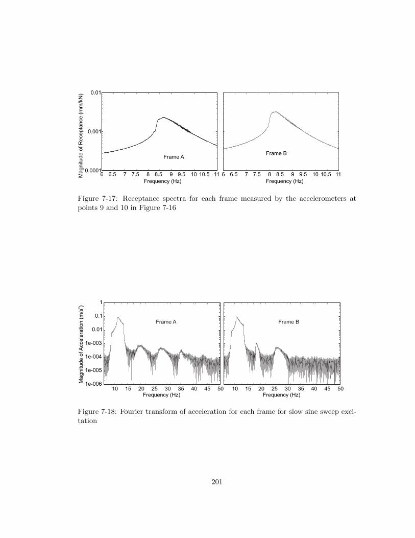
6 6.5 7 7.5 8 8.5 9 9.5 10 10.5 110.0001
0.001
0.01
Frequency (Hz)
Magnitude o
f R
ecepta
nce (
mm
/kN
)
6 6.5 7 7.5 8 8.5 9 9.5 10 10.5 11
Frequency (Hz)
Frame AFrame B
Figure 7-17: Receptance spectra for each frame measured by the accelerometers atpoints 9 and 10 in Figure 7-16
10 15 20 25 30 35 40 45 501e-006
1e-005
1e-004
1e-003
0.01
0.1
1
Frequency (Hz)
Magnitude o
fA
ccele
ration (
m/s
)2
10 15 20 25 30 35 40 45 50Frequency (Hz)
Frame A Frame B
Figure 7-18: Fourier transform of acceleration for each frame for slow sine sweep exci-tation
201

7 7.5 8 8.5 9 9.5 100
0.001
0.002
0.003
0.004
0.005
0.006
0.007
Frequency (Hz)
Magnitude o
f R
ecepta
nce (
m/N
)3.8N
7.6N
11.3N
15.1N
7 7.5 8 8.5 9 9.5 10Frequency (Hz)
F =rms
F =rms
F =rms
F =rms
8.9N
17.6N
26.4N
35.0N
F =rms
F =rms
F =rms
F =rms
Figure 7-19: Receptance spectra for frame B measured by the accelerometer at point10 in Figure 7-16, showing the variation of receptance with amplitude of applied force -the left hand graph is for pseudo-random excitation and the right hand graph for slowsine sweep
the magnitude of the receptance. It should be noted that the fact that the receptance
reduced with amplitude of applied force did not mean that the amplitude of vibration
reduced, merely that it did not increase in proportion with the applied force.
The results of modal analysis of the frame system therefore corresponded qualita-
tively to the single dowel connection tests, in that stiffness was observed to reduce with
increasing amplitude of applied force, with a simultaneous increase in damping.
In the same way as for the cantilever beam specimens, the circle-fit method could be
used to estimate the natural frequency and damping in each of the tests with pseudo-
random excitation. Figure 7-20 shows the process. The noise in the receptance, calcu-
lated according to the method in Section 7.2.1, is thought to be due to the nonlinearity
in the frame, rather than an inadequate averaging time. Since the pseudo-random
excitation continually causes the structure to vibrate at a range of amplitudes, the
receptance of the system will continually change, which may explain the unevenness of
the calculated receptance. Despite this noise, a reasonably consistent range of damping
estimates can be made, as shown in d in Figure 7-20, with the exception of the values
very close to the natural frequency, where the noise has a disproportionate effect on
the estimate. This suggests that the natural frequency estimate is accurate, and gives
a reliable estimate of the damping in the frame.
The slow sine sweep, pseudo-random and impulse excitation methods covered a
range of amplitudes of applied force, and therefore of acceleration in the structure.
Table 7.5 combines the results from the three forms of excitation, for the tests in which
it was possible to extract modal parameters.
Pseudo-random excitation was applied at four amplitudes for each frame, but, as
202

8.89
9.29.4
9.69.8
7.88
8.28.4
8.6
0
1
2
3
4
5
Frequency Abovef (Hz)n
Dam
pin
g R
atio (
%)
Frequency Belowf (Hz)n
8 8.5 9 9.5 10
2
4
6
8
10x 10
-5
Frequency (Hz)
Magnitude o
f R
ecepta
nce H
(f)
(m/N
)x
MagnitudeLimits for analysis
-2 -1 0 1 2 3 4x 10
-5
-5
-4
-3
-2
-1
0
x 10-5
Nyquist Plot with Circle Fit
Real(H (f))x
Imag(H
(f))
x
7.5 8 8.5 9 9.5 10-7
-6
-5
-4
-3
-2
-1
0
frequency (Hz)
Angle
radia
ns
θ
f =8.81Hz atn
=-3.62 radiansθr
a b
cd
Figure 7-20: Modal analysis of frame B, under pseudo-random excitation, by the circle-fit method, using the input force calculated using the accelerometer at point 11 andthe acceleration measured at point 9: a shows the receptance, b the circle-fit to thatreceptance data, c the variation of angle around the circle with frequency and theresulting estimate of natural frequency and d the plot of damping estimates using thatnatural frequency
203

Table 7.5: Modal properties of frames by impulse, pseudo-random (P-R) and slow-sine-sweep excitation, RMS stands for root mean square
Test Excitation RMS R-ratio at Natural Equivalentforce resonance frequency viscous
damping(N) (Hz) (% of
critical)
Frame A AI3 Impulse 2.2 - 10.0 0.5AN0 5a P-R 3.8 - 9.4 2.1AN1 P-R 7.6 - 9.2 2.4AS0 25a Sweep 10.8 1.38 9.5 3.0AS0 5 Sweep 21.6 1.65 9.3 3.7AS0 75 Sweep 32.7 1.90 9.2 4.3AS1 Sweep 43.2 2.23 9.1 4.5
Frame B BI5 Impulse 2.6 - 9.1 1.2BN0 5a P-R 3.8 - 8.8 2.1BN1 P-R 7.6 - 8.7 2.2BS0 25a Sweep 10.8 1.42 8.9 2.5BS0 5 Sweep 21.7 1.69 8.9 3.0BS0 75 Sweep 32.6 2.16 8.7 3.2BS1 Sweep 43.3 2.66 8.6 3.6
was the case for the two-dowel cantilever beams, it was not possible to extract modal
parameters from all of these tests. In the case of the frames, the higher two amplitudes
of applied force resulted in a systematic variation in the damping estimate across the
range of frequencies tested, so that neither a damping estimate nor an accurate estimate
of natural frequency could be made.
Similarly, in several of the impulse tests, a systematic variation was found in the
damping matrix. This was thought to be a result of the quality of the impulse applied,
rather than a high degree of nonlinearity, since it was possible to extract modal infor-
mation from one of the impulse tests on each frame, and they are presented in Table
7.5.
The common reference used to compare the three methods of excitation in Table
7.5 is the root-mean-square (RMS) of the time-series of force applied to the structure.
The excitation and response for each form of excitation is inherently different, so it is
not considered that a pseudo-random and a slow-sine-sweep test, for example, with the
same RMS amplitude of force should give exactly the same modal properties for the
non-linear system. It is, however, considered to be a suitable approximate measure of
the magnitude of each test. The three excitation modes cover a range of RMS force
204

from just over 2N to just over 43N.
For the slow-sine-sweep tests, since the full resonance is allowed time to develop, it is
possible to measure the peak acceleration at resonance and assign an R-ratio according
to (7.21). The natural frequency of the frame varies from 10.0Hz to 9.1Hz for frame A,
and from 9.1Hz to 8.6Hz for frame B, though it should be noted that the magnitude of
the excitation force has been increased by approximately twenty times for this change
to occur.
As in the cantilever beam tests, the frame with the higher stiffness also had the
higher damping, though the difference between the two frames was not as great as the
difference between the two cantilever beams. In the frames, all of the steel plates slid
freely into the slot during assembly; none of them required any force to insert as in the
case of connection A. The results do suggest, however, that a similar process of friction
between the steel plate and the timber may be responsible for the higher stiffness in
frame A, and it is certainly likely that the plates were forced to one side of the slot
during installation of the dowels, and this could generate the normal force required for
this friction to develop.
7.5 Comparison with theoretical predictions
The stress function approach for the stiffness of a moment connection, as presented
in Section 6.3, was used to assign a stiffness to each dowel in each connection. The
orientation of the load on each connector was assumed to be at right angles to the
radial line between the connector and the centroid of the connection. This meant
that dowels in the the two-dowel cantilever connections were assumed to be loaded
parallel to the grain, while in the four-dowel connections in the frames, the dowels
were all loaded at 30◦ to the grain direction, and the additional two dowels in the
six-dowel connection were loaded perpendicular to the grain. For those dowels loaded
at 30◦ to the grain, Hankinson’s formula (Hankinson; 1921) was applied to interpolate
between the calculated foundation moduli parallel and perpendicular to grain. The
appropriateness of this formula for the task was discussed in Section 2.2.5.
The material properties used were based on the material characterization tests for
Norway spruce described in Section 5.4. The specimens for determination of the elastic
modulus were therefore taken from the same batch of glued-laminated timber used
for construction of the cantilever and frame specimens, but were not taken from the
cantilever and frame specimens themselves. The density of the timber for self-weight
was determined by weighing the cantilever beam specimen.
The modal analysis was carried out using the stiffness-matrix model described in
205

joints = 0.87
beams = 0.13
Connections tostrong wall Location of
shaker andapplied mass
Circles represent themagnitude of the workdone in each element
Proportion of work in {
Structure
Node
Mode shape
Natural frequency = 10.6Hz
Modal mass = 170.1kg
Figure 7-21: Mode shape of the fundamental mode of vibration for the frame, withcircles indicating the magnitude of the work done in each element of the structure asit vibrates
Section 7.3.2, which calculated the mode shape, natural frequency, and the distribution
of elastic work done in the structure for each mode of vibration.
Figure 7-21 shows the mode shape for the fundamental mode for the frame, along
with the modal properties. Circles are drawn half way between each pair of nodes to
represent the magnitude of the work done in the element or connection between the
nodes. In total, for this frame, 87% of the total work done on the structure by the
vibrating mass was predicted to be transferred into strain energy in the connections. As
a result, the energy dissipation in the connections was expected to provide the majority
of the energy dissipation in the structure as a whole, and the damping ratio in the
structure as a whole was expected to be similar to that for an individual connection.
In the cantilever joint, 85% of the work was done in the connection, with the remainder
done in bending the beam, for the case of the six-dowel connections. This rises to 87%
for the two-dowel connections. The contribution of the connections to damping in each
structure was therefore expected to be similar, and this was reflected in the similar
range of damping ratios observed in all the cantilever beam and frame tests, with the
exception of the low damping in the impulse tests on the frames, though to be the result
of the extremely low amplitude of vibration, and the high damping in connections A2a,
A2b and A6, thought to be due to the higher friction between the steel plate and the
timber around it.
Having carried out the same theoretical modal analysis for each of the structures,
the predicted natural frequency could be compared with the range of natural frequencies
206

Table 7.6: Comparison of predicted natural frequency with the range of natural fre-quencies measured in tests on each cantilever and frame structure
Structure Predicted Label Measuredfrequency frequency
range(Hz) (Hz)
Cantilever beams 8.7 A2a 10.8-11.1A2b 10.2-10.7B2a 8.0-8.6B2b 8.6-8.7
7.7 A6 8.6-9.4B6 8.2-8.4
Frame 10.6 A 9.1-10B 8.6-9.1
measured during the tests. The results are shown in Table 7.6.
If the connectors were perfectly aligned with the centre of each hole and there was
no significant normal force, and therefore no significant friction between the steel plate
and the timber, then it would be expected that the predicted frequency would be at
the upper part of the range of measured frequencies. This is because the prediction is
based on an elastic analysis, and the results in previous chapters have shown that the
secant stiffness is predicted well by an elastic analysis for small-amplitude oscillation,
but reduces as the amplitude of oscillation increases. This is seen in the results for
the two-dowel moment connections B2a and B2b. The much higher frequencies in A2a
and A2b, as discussed in Section 7.4.1, are thought to be a result of the tightness
of fit between the steel plate and the slot in the timber and the resulting friction.
This unintentional outcome of the cantilever beam tests is of relevance to structural
engineering design, in that it suggests that systems, such as prestressed bolts, which
could provide reliable friction of this form, could be used to improve the performance
of dowel-type connections under in-service vibration.
The two-dowel connections with a loose fit between the steel plate and the slot
therefore perform approximately as predicted. The six-dowel connections do not behave
as predicted. Again, the frequency of connection A is higher than that of connection
B, but in this case even the frequency of connection B is significantly higher than
predicted. The result is sensitive to the angle to grain at which the outer connectors
are loaded or, in the same sense, to the interpolation between the known parallel- and
perpendicular-to-grain stiffnesses: using an angle of 20◦, for example, instead of 30◦,
results in a predicted frequency of 8.4Hz. It is acknowledged that a more rigorous
207

approach to predicting the variation of stiffness with angle to grain is required.
In the predicted stiffness of the six-dowel connection, the outer four dowels con-
tribute 95% of the stiffness of the connection. The fact that the measured stiffness
is higher than the predicted value therefore suggests that at least these outer four
dowels are contributing fully to the moment resistance of the connection. The pro-
cess of preloading, therefore, appears to have allowed any misalignment of the dowels,
which would result in some remaining unloaded or less loaded than the simple analysis
predicts, to be taken up, distributing the force evenly between the dowels.
Comparison of the predicted and measured stiffness of the frames given in Table 7.6
shows that the measured frequency of the frame is slightly lower than predicted in each
case. This may be a result of the lower initial loading as a proportion of the capacity of
the connection. The results in Chapter 5 show that the stiffness of connectors loaded
to 20% of their predicted yield strength fell below the elastic value. In the frame, as
described in Section 7.3.2, while the connections to the laboratory wall were loaded
to approximately 20% of their predicted yield force, the connections between members
were only loaded to approximately 10%. It is therefore considered reasonable that their
stiffness would be lower as a result.
As a simple comparison, the connection stiffness given by Eurocode 5 (BSI; 2009a)
in the form of the slip modulus Kser, when applied to generate the semi-rigid con-
nection stiffness for the frame, predicts a natural frequency of slightly over 6Hz. This
substantial underprediction is due to the fact that the slip modulus allows for all of
the components of deflection from initial loading, including the initial deflection due to
plastic behaviour in the contact surface between dowel and timber, which was shown
in Section 6.6.2 to lead to a stiffness 3.8 times lower than the stiffness under oscillating
load with R=1.2, as an average of the tests presented in that section.
7.5.1 Energy dissipation
It was shown in Section 6.5 that an insight into the equivalent viscous damping ratio for
the single-dowel connection test specimens could be gained by calculating the energy
dissipation due to friction around the face of the dowel. It was found that the energy
dissipation through that mechanism contributed a large proportion of the damping
measured in many of the tests, although there was also evidence of energy dissipation
due to other processes which were not modelled.
Using the same method presented in Section 6.5, it was possible to predict the
damping ratio expected to result from around-the-dowel friction, and this was done for
the two-dowel moment connections. The calculation, as shown in Table 7.7, resulted in
a predicted damping ratio of 0.6%. Table 7.4 shows that the measured damping ratios
208

Table 7.7: Predicted damping by around-the-dowel friction for two-dowel connection
Wi γi
Embedment Hole shape 18.9% 2.9%Rigid insert 49.0% 0.0%
Dowel deformation 22.1% 0.0%Beam deformation 10.0% 0.0%Total γ 0.6%
for the two-dowel connections ranged from 2.40% to 9.00%, which suggests that other
processes are responsible for the majority of the energy dissipation in those connections.
The difference in damping between the connections in which the steel plate fitted
tightly into the slot and those in which there was a looser fit suggests that friction
between the steel plate and the timber around it may be responsible for at least part
of the additional damping which was observed. In this study, there was insufficient
experimental evidence to test any prediction of energy dissipation by this mechanism,
since the force between the timber and the steel plate was not quantified. The analysis
of the energy dissipation in the connection and frame structures was therefore limited
to qualitative discussion.
The damping ratios measured in the frames and cantilever beams are higher than
those in the embedment and single-dowel connection tests. This is considered likely to
be due to friction between the steel plate and the timber. In the single-dowel connection
tests, the loading machine held the steel plate vertically and applied a purely vertical
load through the plate to the dowel. In the frame and cantilever-beam tests, the
structures were unrestrained in the horizontal direction, and so the restraint against
lateral movement was provided by contact between the steel plate and the timber,
consequently leading to the friction forces which were thought to contribute to the
additional measured energy dissipation. It is uncertain whether this friction would
develop in a complete, fully-braced structure.
7.6 Summary
Experimental modal analysis of simple structures with dowel-type connections has
shown that their stiffness and energy dissipation follows a similar pattern to that of the
embedment specimens and single-dowel connections considered in previous chapters.
An additional contribution to both stiffness and energy dissipation has been suggested,
which is the friction between the steel flitch plate and the sides of the timber slot into
which it is inserted. In a connection with a snug fit between the plate and the slot,
209

this effect has been seen to approximately double the energy dissipation, and increase
the stiffness by approximately a fifth.
This source of energy dissipation appeared to be far more substantial than the
around-the-dowel friction predicted according to the method described in the previous
chapter, and a predictive model for this additional form of energy dissipation was
considered to be beyond the scope of this study. The apparent influence of this interface
friction on energy dissipation is a potential topic for further research, however, and it
may be possible to produce highly dissipative connections for in-service conditions by
creating the appropriate conditions for friction between those two surfaces.
An established formulation by Duffing (1918) was used to develop a curve-fitting
approach to analyse the nonlinear response of the cantilever beams and frames to slow-
sine-sweep excitation. Duffing’s formulation was for a particular form of nonlinearity,
cubic stiffness, which was seen to describe parts of the receptance of the systems, but
could not be fitted to the response over its full range of excitation. Nonetheless, by
fitting the cubic stiffness response to the measured receptance, modal parameters such
as the underlying linear natural frequency and the damping could be estimated, where
approaches designed for linear systems failed to provide estimates.
The method used to predict the natural frequencies of the structures took the stiff-
ness calculated according to the stress-function and beam-on-elastic-foundation model
from Chapter 6 and applied the conventional approach to modelling the stiffness of
moment connections and frames. The predicted natural frequency matched the mea-
sured natural frequency well for the smallest amplitude of applied dynamic load, and
for the simplest form of connection, the two-dowel moment connection. Based on
the behaviour of the six-dowel moment connection, it appeared that either the simple
approach to determination of the embedment angle for each connector, or the inter-
polation between parallel- and perpendicular-to-grain stiffness, may be inappropriate.
A reliable calculation for the effect of angle to grain requires further analytical and
experimental study.
The same effect is assumed to be present in the frame specimens, but their measured
natural frequency is, in fact, slightly lower than the predicted value. This is thought to
be due to the low loads, as a proportion of their yield strength, on some of the connectors
in the frames. Despite these inaccuracies, the elastic model gives a reasonable prediction
of the natural frequency of both the cantilever and frame structures, based on the
elastic properties of the timber and the steel, the geometry of the structure and its
mass distribution.
The process of modelling and analysing these structures therefore shows that a
nonlinear variation of stiffness with amplitude of load in each connector appears to be
210

superimposed on an underlying elastic behaviour which can be predicted by the elas-
tic stress-function model for embedment in conjunction with conventional connection
design methods.
211

212

Chapter 8
Application to Example
Structure
In this study, the structural processes which determine the dynamic stiffness of dowel-
type connections have been observed and modelled, starting with the basic component
of a dowel type connection, the embedment of a circular dowel into a piece of timber,
and building up to a complete frame with moment connections formed of four and six
dowels. The analytical methods which have been found to give a good prediction of
the stiffness under certain conditions have been simplified to form a design method
suitable for the calculation, without specialist software, of the natural frequency, under
one-sided in-service vibration, of frames joined by steel dowels.
In this chapter, that design method will be documented and applied to the tall
timber building example used in Chapter 4. In that chapter, the method given in
Eurocode 5 (BSI; 2009a) was used to predict the connection stiffness for analysis of the
along-wind vibration response of the structure. It has been shown in this study that
the Eurocode 5 method greatly underestimates the stiffness of a connection under this
form of vibration.
8.1 Summary of design method
Separate parts of a design method to calculate this stiffness have been presented in
Chapters 6 and 7. They can be combined to give a method for calculating the stiffness
of a complete connection based on its geometry and the material properties of the steel
and timber, which is as follows.
• The local deformation due to the change in the hole shape under load, referred to
as the hole-shape deformation, is estimated. This is done using the stress function
213

Table 8.1: Hole-shape stiffnesses for the GL28h class given in EN 1194 (BSI; 1999)
Load orientation Stiffness for local deformation(N/mm)
Parallel to grain 6581Perpendicular to grain 2190
in Section 6.1.2 but, since it is independent from the geometry of the connection,
could be tabulated for standardized timber properties such as those in EN 338
(BSI; 2009b) for solid timber or EN 1194 (BSI; 1999) for glued-laminated timber.
• The deformation due to the movement of the dowel through the timber, referred
to as the rigid-insert deformation, can be calculated using the simplified method
given in Section 6.3, using (6.59) for a linear applied force and (6.60) for a moment.
• The total stiffness calculated from (6.61) is then used as the foundation modulus
for a beam-on-elastic-foundation calculation representing a single connector under
the given loads.
• The stiffness of a single connector is multiplied by the number of connectors for
a linear applied force, or combined according to (7.18) for a moment.
• The resulting linear and rotational stiffness is applied as a semi-rigid connection
stiffness in the appropriate degrees of freedom of a stiffness-matrix model for the
complete structure, which can be used for modal analysis.
8.2 Calculations
8.2.0.1 Hole shape deformation
It is assumed that the structure will be made from glued-laminated timber complying
with the GL28h classification in EN 1194 (BSI; 1999). The material properties can
therefore be taken to be those given in that standard. The deformation due to change
in hole shape can therefore be calculated for parallel- and perpendicular-to-grain em-
bedment, and the results are shown in Table 8.1.
8.2.0.2 Rigid-insert deformation
In contrast to the hole-shape stiffness, the rigid-insert deformation depends on the
geometry of the connection and the structure. For the translational stiffness of the
connection, the rigid-insert stiffness depends on the length of the member between
214

Table 8.2: Translational rigid-insert stiffness for each dowel in the braced frame of theexample structure
StiffnessParallel Perpendicular
Length N/mm N/mm
14m 62773 1736016m 62014 17154
Table 8.3: Geometry for the example connection: cx is the horizontal distance of thedowel from the centroid in mm, cy the vertical distance in mm and the table shows theradial distance in mm
cx120 60 0 60 120
cy 200 233 209 200 209 233100 156 117 100 117 156
0 120 60 0 60 120100 156 117 100 117 156200 233 209 200 209 233
connections. The length of the members in the braced frame of the example structure
is 16m for the vertical members and 14m for the diagonals. The calculated stiffness is
shown in Table 8.2, showing that the difference in length makes a negligible difference
to the translational stiffness of the connection.
While the lateral loads are resisted primarily by truss action in the frame, the
rotational stiffness of the connections is included for completeness, and to illustrate
the method for their calculation. For the rotational stiffness of the connection, the
rigid-insert stiffness of each dowel depends on its distance from the centroid of the
connection. The geometry of the connection is summarized in Table 8.3, in which each
of the 25 dowels is assigned cx and cy coordinates relative to the centroid, and the radial
distance from the centroid is tabulated for each. cx is the distance from the centroid
in the parallel-to-grain direction, and cy the distance in the perpendicular-to-grain
direction.
Using these radial distances, rigid-insert stiffness can be calculated according to the
simplified method in Section 6.3.
The foundation modulus for calculation of the stiffness of a single connector can
then be found. The stiffness associated with the rigid-insert deformation of each dowel
for this rotational movement can then be added to the stiffness associated with the
hole-shape deformation, and corrected for the angle to the grain given by tan−1(cx/cy).
215

Table 8.4: Foundation moduli, corrected for angle to grain, for each dowel inN/mm/mm
cx120 60 0 60 120
cy 200 746 1125 1446 1125 746100 513 857 1635 857 513
0 374 447 0 447 374100 513 857 1635 857 513200 746 1125 1446 1125 746
Table 8.5: Stiffness for movement of each dowel relative to the centroid of the connectioncx
120 60 0 60 120
cy 200 50664 67590 79219 67590 50664100 37720 56122 86869 56122 37720
0 28719 32821 0 32821 28719100 37720 56122 86869 56122 37720200 50664 67590 79219 67590 50664
The resulting matrix of foundation moduli is shown in Table 8.4, where the foundation
modulus for each dowel is appropriate to its distance from the centroid and the angle
to the grain at which it is loaded. The variation of the foundation modulus with grain
orientation and distance from the centroid can be seen.
The same process for the translational movement of each dowel results in a foun-
dation modulus of 1060N/mm2 in the parallel-to-grain direction and 191N/mm2 in the
perpendicular-to-grain direction. The stiffness is, therefore, dominated by the rigid-
insert deformation, as can be seen by comparing these values to those in Table 8.1.
8.2.0.3 Beam on elastic foundation
A beam-on-elastic-foundation calculation can then be carried out for each dowel based
on its foundation modulus, to calculate its overall stiffness. For translational movement,
this results in a stiffness of 62773N/mm2 parallel and 17360N/mm2 perpendicular to
grain. For rotational movement, the stiffness for each dowel is given in Table 8.5.
These stiffnesses have been calculated for a single flitch plate, using (6.62). The
connection in the example structure contains four flitch plates, and therefore exhibits
approximately four times this stiffness. This approximation corresponds to current
design guidance for the calculation of the slip modulus for a connection according to
Eurocode 5 (BSI; 2009a).
216

Table 8.6: Semi-rigid connection stiffness for use in the stiffness-matrix model
Stiffness
Translation along the grain 7846595 kN/mTranslation across the grain 2169994 kN/mRotation 136074 kNm/radian
8.2.0.4 Combination
For translational movement, all 25 connectors are assumed to exhibit the same stiffness,
which can be summed to give the total stiffness of the connection.
The combined rotational stiffness of the connectors can be calculated according to
(7.18) from Section 7.3.2, reproduced as (8.1). Thus, the translational and rotational
stiffness of the connections in the example structure has been estimated as shown in
Table 8.6.
Kr =n∑i=1
kc,ir2i (8.1)
8.2.0.5 Stiffness matrix
Using the semi-rigid connection stiffnesses in Table 8.6, the structural analysis could
be carried out in the same way in Section 4.1.3, resulting in a mode shape for the
fundamental mode of vibration as shown in Figure 8-1. The analysis in Section 4.1.3
investigated the wind-induced vibration of a 20-storey braced-frame timber structure,
and found that the effect of connection stiffness, modelled according to the Eurocode
5 method, reduced the natural frequency of the first mode of vibration from 0.52Hz to
0.37Hz, with a consequent effect on the amplitude of vibration in the structure due to
turbulent wind load. Table 4.3, from Section 4.1.3, can now be extended to include the
natural frequency calculated using the method developed in this study to give Table
8.7.
The underestimation of stiffness, and therefore natural frequency, by the Eurocode
5 method BSI (2009a) for this structure is less dramatic than in the case of the portal
frame described in Chapter 7. This is because the connections in this structure are
relatively stiff, even according to the Eurocode 5 method, in comparison to the members
themselves, due to their four steel plates and 25 fasteners per connection. Looking at
a typical 700mm by 700mm glulam corner column, the combined translational stiffness
of the connections at either end, as calculated in this section, is approximately 9 times
higher than the axial stiffness of the member itself.
217

joints = 0.13
beams = 0.87Proportion of work in {
Structure
Node
Mode shape
Natural frequency = 0.50Hz
Circles represent themagnitude of the workdone in each element
Figure 8-1: Mode shape for the fundamental mode of vibration with the connectionstiffness determined according to the method developed in this study
Table 8.7: Natural frequency of the first mode of vibration for the 20-storey glued-laminated timber structure
Truss connection 1st/2nd mode naturalfrequency(Hz)
Fixed 0.54Semi-rigid (Eurocode 5) 0.39Semi-rigid (This method) 0.50
218
The connection stiffness predicted by the method developed in this study is, in fact,
approximately 8 times higher than the stiffness according to the Eurocode 5 method
parallel to grain and 2 times higher perpendicular, but the effect on natural frequency
is far less pronounced, because of the relatively small contribution of the connections
to the overall stiffness.
8.2.1 Energy dissipation
The analysis shows that, for the connection stiffness calculated according to the method
presented in this study, the work done in the connections is 13% of the total work done
in the structure in the fundamental mode of vibration. As a result, the weighted
contribution of the connections to the damping ratio of the complete structure will be
small. If the connections have an independent damping ratio γi of 1.3%, as predicted in
Section 6.5 for single-dowel connections carrying a linear load, then their contribution
to the overall damping of the structure would be only 0.17%. On this basis, the
material damping in the timber and the contribution of non-structural elements would
be expected to form the majority of the damping in the structure. It is not therefore
possible to make a more informed estimation of damping than the range from 0.95%
to 1.9% used in the sensitivity analysis in Section 4.1.3.2. It can be stated that, if
the structure is to exhibit damping in this range, then the contribution of energy
dissipation in embedment to that damping would be expected to be small compared to
other sources of energy dissipation.
It is noted, however, that this structure represents only a single example, and there
may be many other structural forms in which the connections store a greater proportion
of the potential energy in the vibrating structure, and so may contribute more to
the overall damping. The experimental and theoretical work on energy dissipation in
this study has also given rise to tentative suggestions of methods of increasing energy
dissipation in connections for in-service vibration, by using high-friction dowels or by
inducing friction between the steel flitch plates and the timber. If methods such as
these could produce much higher energy dissipation in the connections, then they could
make a significant contribution to the overall damping, even in structures such as this
example, where only 13% of the elastic work is done in the connections.
8.3 Summary
The method developed in Chapters 6 and 7 for calculating stiffness in dowel-type con-
nections under in-service vibration has been applied to an example structure, a 20-
storey braced-frame. The structure, as described in Section 4.1.3, was the result of
219

a preliminary design by Norwegian engineers Sweco (Reid; 2009), who published the
member sizes for the main members. The form of the connections, though not their ge-
ometry, was taken from a bridge designed by the same engineers (Abrahamsen; 2008),
using dowel-type connectors with multiple steel flitch plates.
The results showed that the connections were relatively stiff in comparison to the
members they connected, but that the method developed in this study still resulted in
a substantial difference in the calculated natural frequency of the building, compared
with the only method currently open to an engineer designing according to Eurocode
5 (BSI; 2009a), the slip modulus Kser.
There remain some simplifications in this example calculation, which are not con-
sidered to affect these conclusions, but should be noted nonetheless. One is that the
four-plate connection will not, in general, exhibit four times the stiffness of the con-
nection with a single plate. The true stiffness will depend on the spacing of the plates
and the dimension of the member into which the connector is inserted. By representing
the connector as a beam on elastic foundation, the method presented here allows this
geometry to be taken into account.
In a multiple-dowel connection, all the dowels may not exhibit their full stiffness
according to the infinite-plate solution which underlies the stress function used here.
Interaction between the deformation fields around each dowel may result in a lower
stiffness for a group of dowels. This is considered to be an area for further study.
The analysis in this chapter has demonstrated that the results of this study can
have a significant influence on the design of cutting-edge timber structures which use
dowel-type connections, such as a 20-storey building with a glued-laminated timber
frame. The result is to show that, for in-service vibration, the connections exhibit far
higher stiffness than existing empirical design methods allow for.
220
Chapter 9
Conclusion
This study has addressed a shortfall in the understanding of the load-deformation
behaviour of dowel-type connections in timber structures under cyclic loads. It has
focussed on their response to loads representative of in-service vibration, which is taken
to mean vibration as a result of loads which a structure experiences regularly under
normal use. Under this type of dynamic load, the structure should behave in such a
way that ensures the comfort of the occupants, and allows all the systems housed in
the building to perform their function unhindered by any structural movement.
The published performance criteria defining acceptable levels of structural vibration
have been reviewed, and compared against published results of vibration tests on timber
structures and a theoretical analysis of a proposed multi-storey timber structure. These
results showed the sensitivity of timber structures to this form of vibration, highlighted
the lack of knowledge of the behaviour of their connections under such conditions, and
allowed the design of dynamic load tests to mimic the form of load applied to the
connections of structures vibrating in service.
Cyclic load tests and modal analysis were carried out on embedment specimens,
single-dowel connections, moment connections and complete frames. Most of the tests
applied one-sided loading, with no load reversal, in order to represent a common form
of in-service vibration. Their amplitude was represented by the ratio of the maximum
to the minimum load, the R-ratio.
The larger-amplitude R=10 tests generally exhibited lower secant stiffness and
higher energy dissipation than the R=1.2 tests. The reduced stiffness was observed
to be due to nonlinear load-deformation behaviour, in which the stiffness was lower at
lower applied loads, so as the amplitude increased and the minimum of the cyclic com-
ponent was closer to zero, the secant stiffness was reduced. This was considered to be a
result of the imperfect contact surface between dowel and timber, being responsible for
221

a component of deformation under low loads. The higher energy dissipation was also
considered to be due to this contact surface, and the dissipative crushing and buckling
of the microstructure of the timber inherent in its deformation.
It was shown that the stiffness of the timber in embedment by a dowel at R=1.2
could be predicted with reasonable accuracy using an elastic orthotropic stress-function
model, the results of which could then be used to predict the stiffness of single-dowel
connections, where the deformation of the connector was modelled as a beam on elastic
foundation.
Two forms of the stress function, developed by other researchers for investigation of
the stress distribution around pin-loaded holes in orthotropic plates, were reviewed with
the aim of using them to calculate deformations in the material around the hole. As part
of this study, it was shown that by translating and superimposing the stress function
on itself, the geometries of connections subject to linear forces and moments could be
represented. The relative displacements of connectors could then be calculated, which
could be used as the foundation modulus in the beam-on-elastic-foundation model for
the complete connector.
It was noted that such an analytical model would be most useful in the context
of timber engineering if it could be used to derive equations which could be used in
design. It was shown that, using certain simplifying assumptions about the physical
behaviour of the connection and some mathematical approximations, the equations
defining the stress function could be expressed as a concise set of formulae for the
relative deformation of connectors.
The analytical model for embedment was also used for investigation of the mecha-
nisms by which energy was dissipated under cyclic load. It was shown that a particular
dissipative process, that of friction around the dowel as it embeds into the timber,
could be predicted, and appeared to represent a significant part of the total energy
dissipation in the embedment specimens, and in the single-dowel connections. In the
multiple-dowel moment connections in the cantilever beams and frames, other dissipa-
tive mechanisms appeared to be more prevalent.
The contact surface between dowel and timber was seen to have a great influence
on the stiffness of the connection. In Chapter 6, by breaking down the deformation in
embedment into its elastic, viscoelastic and plastic components, it was shown that the
stiffness under initial loading was 38% of that for subsequent cyclic load, as an average
of 54 embedment tests for dowels and screws. The reduced stiffness was thought to be
due to the plastic behaviour of small volumes of timber at the interface between dowel
and timber, micro-buckling and crushing irreversibly under initial loading and then
forming a more rigid contact surface under subsequent cycles of load. This hypothesis
222
was justified by microscope images of the timber immediately around the edge of the
hole, which showed micro-buckling of fibres where the timber had been subject to load
parallel to the grain and crushing of trachieds as a result of perpendicular-to-grain load.
The quality of this contact surface would have depended on variables such as the type
of drill bit used and its speed of rotation, which would make it difficult to predict.
Under the small-amplitude movements associated with in-service vibration, the
contribution of viscoelastic and plastic behaviour in the timber to the stiffness of the
connection was observed to become small in comparison to the elastic component. In
those conditions, the method developed in this study, which predicts the magnitude of
the elastic component based on the material properties of the timber and connector,
can therefore be used to predict the stiffness of a single connector.
Having derived the stiffness of a single connector, it was shown that conventional
design methods could be used to express the behaviour of a group of connectors, albeit
with some modification to allow for the fact that the stiffness of each connector may vary
depending on their position in the geometry of the connection. It was therefore possible
to predict the stiffness of a multiple-dowel connection, and then, using a stiffness-matrix
method, a complete frame.
The nonlinear effect of the contact surface between dowel and timber was observed
throughout the experimental investigation, and was evident in the modal analysis of two
simple structural forms, a cantilever and a portal frame, with dowelled connections. The
nonlinear stiffness in the connections resulted in an amplitude-dependence of stiffness
in the cantilever and frame. A curve-fitting approach was developed, based on the
theory of an oscillator with cubic stiffness, which allowed assessment of the damping
in these structures. It was shown that the assumption of cubic stiffness did not fit
the response of the structures well over a range of amplitudes, but could be used on a
selected portion of the measured receptance for estimation of the modal properties.
This study has therefore traced the behaviour of dowel-type connections under
cyclic loads from the embedment of the dowel into the surrounding timber to the
behaviour of a complete frame. Methods have been developed to analyse and quantify
the experimental results at each scale, and a calculation process has been derived to
predict the linear part of the response of a connection based on the elastic properties
of the timber and connector.
This nonlinear response has consequences for design, in-situ testing and analysis of
timber structures for vibration, since it means that the natural frequency and damping
in a structure can be expected to vary with the amplitude of vibration. In the inves-
tigation into in-service vibration described in Chapter 4, it was shown that in-service
vibration in structures often consists of a resonant response resulting in oscillating loads
223

on connections with an R-ratio between 1 and 1.2. It was then shown that an elastic
model predicted the stiffness of the connections well for that range of R-ratios. The
elastic design would not be appropriate, however, for vibration at a higher amplitude,
or with load reversal, and it has been shown that the stiffness in dowel-type connections
under such conditions is much lower, and is accompanied by an increase in damping.
This is also a consideration for modal testing of structures, since it means tests carried
out at a certain amplitude of vibration would not necessarily be representative of the
response at other amplitudes.
A design procedure was developed to allow calculation of this elastic stiffness, and
the calculation was carried out for an example structure, a 20-storey building with a
frame of glued-laminated timber. This example highlighted the effect that connection
stiffness can have on the response of a full-scale building structure to in-service dynamic
loads such as wind, and showed that the design procedure could be used to predict that
amplitude of the additional forces imposed on structural components by vibration, and
the amplitude of acceleration which would be imposed on the building’s occupants.
9.1 Potential further work
Given a reliable theory for prediction of the elastic component of deformation in a
connection, there is also potential to predict the deformation including viscoelastic and
plastic components based on fundamental properties of the material rather than em-
pirical relationships. This is an area for further research, and is considered to be a
tractable problem, given that, under loads below the yield strength of the connection,
the majority of plastic deformation is thought to be in the compaction of the contact
surface between dowel and timber. Further study could include measurement of prop-
erties of the contact surface prepared by different drilling techniques and their effect
on that component of the deformation in the connection.
The viscoelastic component of deformation has been addressed in this study, pro-
ducing a rheological model applicable to a particular range of movement, but further
research could develop a more generally applicable model. If the three components of
the dowel deformation: elastic, plastic and viscoelastic, could be separately predicted,
this would lead to a method which could be applied at a range of serviceability limit
states in design, including vibration in-service, as in this study, but also differential
movement under variable loads and total deformation. This would result in more effi-
cient design of connections in timber structures, and therefore in more efficient design
of complete structures.
This study uses plain dowels and screws made of steel, but it is considered that
224

the experimental and theoretical methods developed could be applied, with further
research to determine appropriate parameters, to other materials. The materials and
forms of connector could be chosen to enhance energy dissipation or reduce initial slip.
The results presented in Section 6.6 broke down the deformation in embedment over
a 16-minute period into its elastic, viscoelastic and plastic components, and found that
a large part of the initial deformation was likely due to local plastic compression of the
contact surface between dowel and timber. This result suggests that there is potential
to greatly increase the stiffness of such connections by improving the surface of the
timber with which the dowel makes contact. The drilling process has been seen to
leave a rough surface which compresses irreversibly under initial loading. An improved
drilling method could therefore reduce this deformation. Another possibility would be
a process in which the hole was drilled to a smaller diameter, and the contact surface
pre-compressed to reduce the residual plastic deformation. On the structural scale,
pre-stressing could be used to ensure that load reversal does not occur, and the contact
surface remains compressed in the range of in-service forces and displacements.
The theoretical investigation of energy dissipation in Section 6.5 showed the poten-
tial for the friction around the dowel as it embeds into the timber to strongly influ-
ence the energy dissipation in embedment. This suggests that a high-friction interface
between dowel and timber could improve energy dissipation in the connection and
therefore damping in the structure as a whole. Experimental investigation would be
necessary to validate this theoretical prediction, and to find the dowel material or sur-
face preparation which could have a suitable interaction with the timber at the hole
edge.
Similarly, in the cantilever beams and frames tested, friction between the steel
connecting plate and the timber was considered to provide a substantial amount of
energy dissipation. It therefore seems reasonable that an appropriate compressive force
between the plate and the timber, perhaps applied by bolts tightened to a specified
level, could result in a highly dissipative connection.
225

226

Bibliography
Abrahamsen, R. (2008). Bridge across Rena River - “World’s strongest timber bridge”,
World Conference of Timber Engineering, Miyazaki, Japan.
Adalian, C. and Morlier, P. (2002). “Wood Model” for the dynamic behaviour of wood
in multiaxial compression, Holz als Roh- und Werkstoff 60(6): 433–439.
Airy, G. B. (1863). On the strains in the interior of beams, Philosophical Transactions
of the Royal Society 153: 49–80.
Aluko, O. and Whitworth, H. A. (2008). Analysis of stress distribution around pin
loaded holes in orthotropic plates, Composite Structures 86(4): 308–313.
Armstrong, L. D. and Kingston, R. S. T. (1960). Effect of moisture changes on creep
in wood, Nature 185(4716): 862–863.
ASTM (1997). Standard test method for evaluating dowel-bearing strength of wood
and wood-based products (reapproved 2002), Technical Report D5764-97a, ASTM.
Atack, D. and Tabor, D. (1958). The friction of wood, Proceedings of the Royal Society
of London. Series A, Mathematical and Physical Sciences 246(1247): 539–555.
Baber, T. T. and Noori, M. N. (1986). Modeling general hysteresis behavior and
random vibration application, Journal of Vibration Acoustics Stress and Reliability
in Design 108(4): 411–420.
Bachmann, H. (1992). Case studies of structures with man-induced vibrations, Journal
of Structural Engineering 118(3): 631–647.
Bachmann, H. and Ammann, W. (1987). Vibrations in structures: induced by man and
machines, International Association of Bridge and Structural Engineering, Zurich.
Birkinshaw, C., Buggy, M. and Henn, G. G. (1986). Dynamic mechanical analysis of
wood, Journal of Materials Science Letters 5(9): 898–900.
227

Bodig, J. and Jayne, B. (1993). Mechanics of wood and wood composites, Krieger
Publishing Company, Malabar, FL, USA.
Bouc, R. (1967). Forced vibration of mechanical systems with hysteresis, Preceedings of
the 4th International Conference on Nonlinear Oscillations, Prague, Czechoslovakia.
BSI (1991). Timber structures. joints made with mechanical fasteners. general prin-
ciples for the determination of strength and deformation characteristics, Technical
Report BS EN 26891:1991, BSI.
BSI (1999). Timber structures - glued laminated timber, Technical Report BS EN
1194:1999, BSI.
BSI (2002a). Eurocode 0 - basis of structural design, Technical Report BS EN
1990:2002, BSI.
BSI (2002b). Moisture content of a piece of sawn timber, Technical Report BS EN
13183:2002, BSI.
BSI (2005). Eurocode 1 actions on structures part 1-4: General actions - wind actions,
Technical Report BS EN 1991-1-4:2005, BSI.
BSI (2007). Timber structures. test methods. determination of embedment strength
and foundation values for dowel type fasteners, Technical Report BS EN 383:2007,
BSI.
BSI (2008a). Guide to evaluation of human exposure to vibration in buildings, Technical
Report BS 6472-1:2008, BSI.
BSI (2008b). UK National Annex to Eurocode 3: Design of steel structures Part 1-1:
General rules and rules for buildings, Technical Report NA to BS EN 1993-1-1:2005,
BSI.
BSI (2009a). Eurocode 5 design of timber structures part 1-1: General - common rules
and rules for buildings, Technical Report BS EN 1995-1-1:2004+A1:2008, BSI.
BSI (2009b). Structural timber. strength classes, Technical Report BS EN 338: 2009,
BSI.
BSI (2011). Timber structures. structural timber and glued laminated timber. de-
termination of some physical and mechanical properties, Technical Report BS EN
408:2010, BSI.
228
Bucher, I. (1991). circfit MATLAB function, http://www.mathworks.co.uk/
matlabcentral/fileexchange/5557-circle-fit/content/circfit.m.
Buffon, G. L. L. D. (1740). Experiences sur la force du bois, L’Academie Royale des
Sciences - Histoire et Memoires pp. 453–467.
Bulıcek, M., Malek, J. and Rajagopal, K. (2012). On kelvin-voigt model and its gen-
eralizations, Evolution Equations and Control Theory 1(1): 17–42.
Burgers, J. M. (1939). Mechanical considerations - model systems - phenomenological
theories of relaxation and of viscosity, First Report on Viscosity and Plasticity, 2nd
edn, N.V. Noord-Hollandsche Uitgevers Maatschappij, Amsterdam, pp. 27–30.
Casado, C. M., Dıaz, I. M., de Sebastian, J., Poncela, A. V. and Lorenzana, A. (2013).
Implementation of passive and active vibration control on an in-service footbridge,
Structural Control and Health Monitoring 20(1): 70–87.
Ceccotti, A. (2008). New technologies for construction of medium-rise buildings in
seismic regions: The XLAM case, Structural Engineering International 18(2): 156–
165.
Charney, F. A. (1990). Wind drift serviceability limit state design of multistory build-
ings, Journal of Wind Engineering and Industrial Aerodynamics 36, Part 1(0): 203–
212.
Chen, J. T. and You, D. W. (1997). Hysteretic damping revisited, Advances in Engi-
neering Software 28(3): 165–171.
Chui, Y. H. and Li, Y. (2005). Modeling timber moment connection under reversed
cyclic loading, Journal of Structural Engineering 131(11): 1757–1763.
Chui, Y. H., Ni, C. and Jiang, L. (1998). Finite-element model for nailed wood joints
under reversed cyclic load, Journal of Structural Engineering 124(1): 96–103.
Chui, Y. and Ni, C. (1997). Load-embedment response of timber to reversed cyclic
load, Wood and Fiber Science 29(2): 148–160.
Clouser, W. S. (1959). Creep of small wood beams under constant bending load,
Technical Report 2150, Department of Agriculture, Forest Service, Forest Products
Laboratory, Madison, WI.
Cobb, F. (2009). Structural Engineer’s Pocket Book, 2nd edn, Butterworth-Heinemann,
Oxford.
229
Coulomb, C. A. (1821). Theorie des machines simples, nouvelle edicion edn, Huzard
courcier, Paris.
Crandall, S. H. (1991). The hysteretic damping model in vibration theory, Journal of
Mechanical Engineering Science 205(13): 23–28.
Daudeville, L., Davenne, L. and Yasumura, M. (1999). Prediction of the load carrying
capacity of bolted timber joints, Wood Science and Technology 33(1): 15–29.
Davenport, A. G. (1961). The application of statistical concepts to the wind loading
of structures, Proceedings of the Institution of Civil Engineers 19(4): 449–472.
De Jong, T. (1977). Stresses around pin-loaded holes in elastically orthotropic or
isotropic plates, Journal of Composite Materials 11(3): 313.
Derdas, C. and Kostopoulos, V. (2011). On the bearing failure of laminated composite
pin-loaded joints: exploitation of semi-analytical solutions for the determination of
the stress state, Strain 47: 320–332.
Dinwoodie, J. M. (2000). Timber its nature and behaviour, 2nd edn, Spon, London.
Dorn, M. (2012). Investigations on the serviceability limit state of dowel-type timber
connections, PhD thesis, Faculty of Civil Engineering, Vienna University of Technol-
ogy.
Dorn, M., de Borst, K. and Eberhardsteiner, J. (2013). Experiments on dowel-type
timber connections, Engineering Structures 47(0): 67–80.
Duffing, G. (1918). Erzwungene schwingungen bei veranderlicher eigenfrequenz und
ihre technische bedeutung, F. Vieweg & Sohn, Braunschweig.
Echavarrıa, C., Haller, P. and Salenikovich, A. (2007). Analytical study of a pinloaded
hole in elastic orthotropic plates, Composite Structures 79(1): 107–112.
Ehlbeck, J. and Larsen, H. J. (1993). Eurocode 5 - design of timber structures: Joints,
International workshop on wood connectors, Forest Products Society, Madison, WI,
USA, pp. 9–23.
Ellis, B. R. and Bougard, A. J. (2001). Dynamic testing and stiffness evaluation
of a six-storey timber framed building during construction, Engineering Structures
23(10): 1232–1242.
230

Eriksson, P.-E. (1994). Vibration of low-frequency floors-dynamic forces and response
prediction, PhD thesis, Department of Civil Engineering, Chalmers University of
Technology.
Ewins, D. J. (1986). Modal testing: theory and practice, Research Studies Press Ltd.,
Baldock, Hertfordshire, England.
Filiatrault, A., Christovasilis, I. P., Wanitkorkul, A. and Lindt, J. W. v. d. (2010).
Experimental seismic response of a full-scale light-frame wood building, Journal of
Structural Engineering 136(3): 246–254.
Filiatrault, A., Isoda, H. and Folz, B. (2003). Hysteretic damping of wood framed
buildings, Engineering Structures 25(4): 461–471.
Foliente, G. C. (1995). Hysteresis modeling of wood joints and structural systems,
Journal of Structural Engineering 121(6): 1013–1022.
Folz, B. and Filiatrault, A. (2001). Cyclic analysis of wood shear walls, Journal of
Structural Engineering 127(4): 433–441.
Forest Products Laboratory (2010). The wood handbook, Technical Report
FPLGTR190, Department of Agriculture, Forest Service, Forest Products Labora-
tory, Madison, WI.
Foschi, R. (2000). Modeling the hysteretic response of mechanical connections for wood
structures, World Conference of Timber Engineering, Whistler, B.C., Canada.
Foschi, R., Yao, F. and Rogerson, D. (2000). Determining embedment response pa-
rameters from connector tests, World Conference on Timber engineering, Whistler,
B.C., Canada.
Goodier, J. N. (1942). An extension of Saint-Venant’s principle, with applications,
Journal of Applied Physics 13(3): 167–171.
Gressel, P. (1984). Zur vorhersage des langfristigen formnderungsverhaltens aus kurz-
kriechversuchen, Holz als Roh- und Werkstoff 42(8): 293–301.
Hankinson, R. (1921). Investigation of crushing strength of spruce at varying angles of
grain, 3(259).
Hearmon, R. F. S. (1961). An introduction to applied anisotropic elasticity, 1st edn,
Oxford University Press, London.
231

Heiduschke, A. (2006a). Analysis of wood-composite laminated frames under dynamic
loads - analytical models and model validation. part i: Connection model, Progress
in Structural Engineering and Materials 8(3): 103–110.
Heiduschke, A. (2006b). Analysis of wood-composite laminated frames under dynamic
loads - analytical models and model validation. part ii: Frame model, Progress in
Structural Engineering and Materials 8(3): 111–119.
Hooke, R. L. (1678). Lectures de potentia restitutiva.
Hunt, D. G. (1999). A unified approach to creep of wood, Proceedings: Mathematical,
Physical and Engineering Sciences 455(1991): 4077–4095.
Hunt, D. G. (2004). The prediction of long-time viscoelastic creep from short-time
data, Wood Science and Technology 38(7): 479–492.
Hwang, K. and Komatsu, K. (2002). Bearing properties of engineered wood products I:
effects of dowel diameter and loading direction, Journal of Wood Science 48(4): 295–
301.
Hyer, M. and Klang, E. (1985). Contact stresses in pin-loaded orthotropic plates,
International Journal of Solids and Structures 21(9): 957–975.
Ingolfsson, E. T., Georgakis, C. T. and Jonsson, J. (2012). Pedestrian-induced lateral
vibrations of footbridges: A literature review, Engineering Structures 45(0): 21–52.
Irwin, A. W. (1978). Human response to dynamic motion of structures, The Structural
Engineer 56(9): 237–244.
Irwin, P. A. and Breukelman, B. (2001). Recent applications of damping systems
for wind response, Proceedings of the Council on Tall Buildings and Urban Habitat,
World Congress, Melbourne, Australia.
ISO (1984). Guidelines for the evaluation of the response of occupants of fixed struc-
tures, especially buildings and offshore structures, to low-frequency horizontal motion
(0.063 to 1.0 hz), Technical Report ISO 6897: 1984, International Organization for
Standardization.
ISO (1990). Method for experimental determination of mechanical mobility - Part 2:
Measurements using single-point translation excitation with an attached vibration
exciter, Technical Report ISO 7626-2:1990, International Organization for Standard-
ization.
232

ISO (2007). Bases for design of structures - Serviceability of buildings and walkways
against vibrations, Technical Report ISO 10137:2007, International Organization for
Standardization.
Jiali, J. and Jianxiong, L. (2009). Anisotropic characteristics of wood dynamic vis-
coelastic properties, Forest Products Journal 59(7/8): 59–64.
Johansen, K. W. (1949). Theory of timber connections, International Association of
Bridge and Structural Engineering 9: 249–262.
Jones, R. M. (1975). Mechanics of Composite Materials, Scripta Book Company, Wash-
ington D. C.
Jorissen, A. (1999). Double shear timber connections with dowel type fasteners, Heron
44(3): 131–161.
Kharouf, N., McClure, G. and Smith, I. (2003). Elasto-plastic modeling of wood bolted
connections, Computers & Structures 81(811): 747–754.
Kimball, A. L. and Lovell, D. E. (1927). Internal friction in solids, Physical Review
30(6): 948–959.
Kuenzi, E. W. (1955). Theoretical design of a nailed or bolted joint under lateral
load, Technical Report D1951, US Department of Agriculture, Forest Service, Forest
Products Laboratory.
Kwok, K. C. S., Hitchcock, P. A. and Burton, M. D. (2009). Perception of vibration
and occupant comfort in wind-excited tall buildings, Journal of Wind Engineering
and Industrial Aerodynamics 97(7-8): 368–380.
Labonnote, N., Rønnquist, A. and Malo, K. A. (2012). Experimental study on material
damping in timber beams, World Conference of Timber Engineering, Auckland, New
Zealand.
Labonnote, N., Rønnquist, A. and Malo, K. A. (2013). Modified hysteretic damping
model applied to Timoshenko timber beams, Computers & Structures 121(0): 22–31.
Leijten, A. J. M., Ruxton, S., Prion, H. and Lam, F. (2006). Reversed-cyclic be-
havior of a novel heavy timber tube connection, Journal of Structural Engineering
132(8): 1314–1319.
Lekhnitskii, S. G. (1968). Anisotropic Plates, 2nd edn, Gordon and Breach, New York.
233

Liang, H., Wen, Y.-K. and Foliente, G. C. (2011). Damage modeling and damage
limit state criterion for wood-frame buildings subjected to seismic loads, Journal of
Structural Engineering 137(1): 41–48.
Maxwell, J. C. (1868). On the dynamical theory of gases, Philosophical Magazine
35: 134.
McKenzie, W. M. and Karpovich, H. (1968). The frictional behaviour of wood, Wood
Science and Technology 2(2): 139–152.
Noguchi, M. and Komatsu, K. (2004). A new method for estimating stiffness and
strength in bolted timber-to-timber joints and its verification by experiments (ii):
bolted cross-lapped beam to column joints, Journal of Wood Science 50(5): 391–
399.
Polensek, A. and Schimel, B. D. (1991). Dynamic properties of light-frame wood
subsystems, Journal of Structural Engineering 117(4): 1079–1095.
Porteous, J. and Kermani, A. (2007). Structural Timber Design to Eurocode 5, Black-
well, Oxford.
Proen ca, J. M. S. F. M. and Branco, F. A. B. (2005). Case studies of vibrations in
structures, Revue Europeenne de Genie Civil 9(1-2): 159–186.
Rainer, J., Pernica, G. and Allen, D. E. (1988). Dynamic loading and response of
footbridges, Canadian Journal of Civil Engineering 15(1): 66–71.
Reid, R. L. (2009). Norwegian team designs world’s tallest timber building, Civil
Engineering 80(8): 26–28.
Resch, E. and Kaliske, M. (2010). Three-dimensional numerical analyses of load-bearing
behavior and failure of multiple double-shear dowel-type connections in timber engi-
neering, Computers & Structures 88(34): 165–177.
Reynolds, T., Harris, R. and Chang, W.-S. (2013a). An analytical model for embedment
stiffness of a dowel in timber under cyclic load, European Journal of Wood and Wood
Products 71(5): 609–622.
Reynolds, T., Harris, R. and Chang, W.-S. (2013b). Viscoelastic embedment behaviour
of dowels and screws in timber under in-service vibration, European Journal of Wood
and Wood Products 71(5): 623–634.
234

Rodd, P. D. and Leijten, A. J. M. (2003). High-performance dowel-type joints for
timber structures, Progress in Structural Engineering and Materials 5(2): 77–89.
Ronnquist, A., Wollebæk, L. and Bell, K. (2006). Dynamic behavior and analysis of
a slender timber footbridge, World Conference on Timber Engineering, Portland,
Oregon.
Santos, C. L., De Jesus, A. M. P., Morais, J. J. L. and Lousada, J. L. P. C. (2009).
Quasi-static mechanical behaviour of a double-shear single dowel wood connection,
Construction and Building Materials 23(1): 171–182.
Santos, C. L., De Jesus, A. M. P., Morais, J. J. L. and Lousada, J. L. P. C. (2010). A
comparison between the EN 383 and ASTM D5764 test methods for dowel-bearing
strength assessment of wood: experimental and numerical investigations, Strain
46(2): 159–174.
Sawata, K. and Yasumura, M. (2002). Determination of embedding strength of wood
for dowel-type fasteners, Journal of Wood Science 48(2): 138–146.
Sawata, K. and Yasumura, M. (2003). Estimation of yield and ultimate strengths of
bolted timber joints by nonlinear analysis and yield theory, Journal of Wood Science
49(5): 383–391.
Schniewind, A. P. and Barrett, J. D. (1972). Wood as a linear orthotropic viscoelastic
material, Wood Science and Technology 6(1): 43–57.
Simiu, E. and Scanlan, R. H. (1986). Wind effects on structures: an introduction to
wind engineering, 2nd edn, Wiley, New York ; Chichester.
Sjodin, J., Enquist, B. and Serrano, E. (2006). Contact-free measurements and nu-
merical analyses of the strain distribution in the joint area of steel-to-timber dowel
joints, European Journal of Wood and Wood Products 64(6): 497–506.
Sjodin, J., Serrano, E. and Enquist, B. (2008). An experimental and numerical study
of the effect of friction in single dowel joints, European Journal of Wood and Wood
Products 66(5): 363–372.
Smith, A. L., Hicks, S. J. and Devine, P. J. (2009). Design of floors for vibration:
a new approach, Technical Report P354, The Steel Construction Institute, Ascot,
Berkshire, UK.
Song, J. and Der Kiureghian, A. (2006). Generalized Bouc-Wen model for highly
asymmetric hysteresis, Journal of Engineering Mechanics 132(6): 610–618.
235
Stevenson, R. (1821). Description of bridges of suspension, The Edinburgh Philosophical
Journal 5: 237–256.
Student (1908). The probable error of a mean, Biometrika 6(1): 1–25.
Sun, N., Das, S. and Frazier, C. E. (2007). Dynamic mechanical analysis of dry
wood: linear viscoelastic response region and effects of minor moisture changes,
Holzforschung 61(1): 28–33.
Thomson, W. (1865). On the elasticity and viscosity of metals, Proceedings of the Royal
Society of London 14: 289–297.
Thorby, D. (2008). Structural dynamics and vibration in practice, Materials & Mechan-
ical, Butterworth-Heinemann, Amsterdam.
Voigt, W. (1892). Ueber innere Reibung fester Korper, insbesondere der Metalle, An-
nalen der Physik 283(12): 671–693.
von Karman, T. and Rubach, H. (1912). On the mechanisms of fluid resistance,
Physikalische Zeitschrift 13: 49–59.
Vural, M. and Ravichandran, G. (2003). Dynamic response and energy dissipation
characteristics of balsa wood: experiment and analysis, International Journal of
Solids and Structures 40(9): 2147–2170.
Wen, Y.-K. (1976). Method for random vibration of hysteretic systems, Journal of the
Engineering Mechanics Division 102(2): 249–263.
Willford, M. R. and Young, P. (2006). A design guide for footfall induced vibration
of structures, Technical Report CCIP-016, The Concrete Centre, Camberley, Surrey,
UK.
Winkler, E. (1867). Die Lehre von der Elasticitaet und Festigkeit mit besonderer Rck-
sicht auf ihre Anwendung in der Technik, fur polytechnische Schulen, Bauakademien,
Ingenieure, Maschinenbauer, Architekten, etc., H Dominicus, Prague.
Zhang, H., Foliente, G. C., Yang, Y. and Ma, F. (2002). Parameter identification
of inelastic structures under dynamic loads, Earthquake Engineering & Structural
Dynamics 31(5): 1113–1130.
Zhang, K.-D. and Ueng, C. E. (1984). Stresses around a pin-loaded hole in orthotropic
plates, Journal of Composite Materials 18(5): 432–446.
236

Zivanovic, S., Pavic, A. and Reynolds, P. (2005). Vibration serviceability of footbridges
under human-induced excitation: a literature review, Journal of Sound and Vibration
279(12): 1–74.
237

238

List of Publications
Chapman, J., Reynolds, T. P. S. and Harris, R. (2012). A 30 level cross laminated
timber building system and anlaysis of the Eurocode dynamic wind loads, World
Conference on Timber Engineering, Auckland, New Zealand.
Reynolds, T., Harris, R. and Chang, W.-S. (2013a). An analytical model for embedment
stiffness of a dowel in timber under cyclic load, European Journal of Wood and Wood
Products 71(5): 609–622.
Reynolds, T., Harris, R. and Chang, W.-S. (2013b). Viscoelastic embedment behaviour
of dowels and screws in timber under in-service vibration, European Journal of Wood
and Wood Products 71(5): 623–634.
Reynolds, T. P. S. (2012). Vibration of timber structures with dowel-type connections,
Young Researchers’ Meeting of COST Action FP1004, Zagreb, Croatia.
Reynolds, T. P. S., Harris, R. and Chang, W.-S. (2011). Dynamic response of tall
timber buildings to wind load, IABSE-IASS Symposium, London, UK.
Reynolds, T. P. S., Harris, R. and Chang, W.-S. (2012). Dynamic stiffness and damp-
ing of dowel-type connections for timber structures under service conditions, World
Conference on Timber Engineering, Auckland, New Zealand.
Reynolds, T. P. S., Harris, R. and Chang, W.-S. (2013c). In-service dynamic stiffness
of dowel-type connections, Meeting of CIB-W18 on Timber Structures, Vancouver,
Canada.
239