dynamic braking industrial electrical engineering and ... document/5292_full... · division of...

Ind

ust

rial E

lectr

ical En

gin

eerin

g a

nd

A

uto

matio

n

CODEN:LUTEDX/(TEIE -5292)/1 -65/(2012)

Dynamic Braking

A new approach for testing Electrical Machines

Eloy Pedro Sánchez Caton

Division of Industrial Electrical Engineering and Automation Faculty of Engineering, Lund University

Fran Marquez

Sticky Note

MigrationConfirmed set by Fran Marquez

Fran Marquez

Sticky Note

MigrationNone set by Fran Marquez

Fran Marquez

Typewritten Text

Fran Marquez

Typewritten Text

Dynamic Braking: A new approach

for testing Electrical Machines

Eloy Pedro Sánchez Caton

February 2012

Supervisor:

Francisco Marquez

Examiner:

Professor Mats Alaküla

Master’s Thesis

Division of Industrial Electrical Engineering and Automation

I

Abstract

In this thesis, a novel method for characterizing Permanent Magnet Synchronous Machines

(PMSMs) based in the dynamic response of the analyzed motor is evaluated. The most

significant motor characteristics -torque, flux and efficiency maps- are computed from the

motor voltage, currents and rotor position data sampled during the experiment. This way of

obtaining the characteristics of the motor is possible thanks to the use of new data acquisition

equipment based on Field-Programmable Gate Arrays (FPGAs) with sampling frequencies up

to MHz, which make possible to calculate the transient state, and not only the steady state

data.

Among the advantages of the evaluated method is that there is no need to couple the test

motor to either a torque measurement device or a braking motor, which reduces both

the required size of the lab and the costs of the test. Moreover, the whole test sequence is

completely automated as well as the post-processing of the experimental results, and it is all

conducted within a few minutes, avoiding the drift in the results originated from the variation

of temperature and other external conditions.

First in this work, a simulation model of the complete test is developed in Simulink, in order

to validate the test protocol. Subsequently, the method is applied to a real Permanent Magnet

Synchronous Motor (PMSM) of known characteristics, in order to evaluate the performance

of the proposed method in relation to more traditional ways of testing electrical machines. .

When compared to the available motor characteristics, the torque and flux maps obtained with

the suggested test method exhibit smoother curves, due mostly to the higher sampling

frequency and accuracy of the new data acquisition process. In addition, the matching

between the newly obtained motor characteristics and those already available is remarkable,

and the slight differences that appear can be explained by the different evolution of the motor

temperature (particularly the rotor magnets’ temperature) throughout the test for the two

methods considered. In conclusion, the results presented in this thesis work prove that the

evaluated method is suitable for characterizing electrical machines.

III

Table of contents

Abstract ..................................................................................................................................... I

Table of contents .................................................................................................................... III

Table of figures ........................................................................................................................ V

Table of tables ......................................................................................................................... VI

Acknowledgments ............................................................................................................... VIII

1. - Introduction ........................................................................................................................ 1

2. - The electric motor .............................................................................................................. 3

2.1 - Background ................................................................................................................................3

2.2 - Classification of Electric Motors ..............................................................................................5

2.3 - Mathematical description ..........................................................................................................7

2.3.1- DC motor model ...............................................................................................................7

2.3.2- AC motor model ...............................................................................................................9

2.3.3- Mathematical description .............................................................................................. 10

2.4 - Mechanical design ................................................................................................................... 13

2.5 - Control of PMSM .................................................................................................................... 15

2.5.1- DCC method:................................................................................................................. 16

2.5.2- PI control method .......................................................................................................... 17

3. - Test method: Description ................................................................................................ 20

3.1 - Description ............................................................................................................................... 20

3.2 - Simulation model .................................................................................................................... 21

3.2.1 - Motor model .................................................................................................................. 21

3.2.2 - PI controller model ........................................................................................................ 22

3.2.3 - Currents reference subsystem ........................................................................................ 23

3.3 - Postprocessing ......................................................................................................................... 24

3.3.1 - Torque map ................................................................................................................... 24

3.3.2 - Flux map ........................................................................................................................ 24

3.3.3 - Losses ............................................................................................................................ 25

3.4 - Lab setup description: Hardware and Software .................................................................. 25

4. - Simulations results ........................................................................................................... 27

5. - Experimental results ........................................................................................................ 30

5.1 - Estimation of the rotating mass inertia ................................................................................. 30

IV

5.2 - Experimental results ............................................................................................................... 33

6. - Comparative study of the results .................................................................................... 36

6.1 - Experimental vs. FE simulations ........................................................................................... 36

6.2 - Experimental vs. verified motor characteristics .................................................................. 38

7. - Conclusions ....................................................................................................................... 41

7.1 - Simulations .............................................................................................................................. 41

7.2 - Simulations vs. experimental results ..................................................................................... 41

7.3 - Experimental vs. verified motor characteristics .................................................................. 41

7.4 - Note on the experimentally obtained motor characteristics ............................................... 42

7.5 - Final conclusion ....................................................................................................................... 42

8. - Further development of the method ............................................................................... 44

9. - References ......................................................................................................................... 45

10. - Appendix: Developed software ..................................................................................... 46

10.1- Torque maps simulation ........................................................................................................ 46

10.2- Flux maps simulation ............................................................................................................. 52

10.3- Postprocessing for torque and flux maps ............................................................................. 52

10.4- Validation script (Lsx, Lsy and Psim) .................................................................................. 54

V

Table of figures

Figure 1: The electric motor model ..........................................................................................................6

Figure 2: 1-pole model .............................................................................................................................8

Figure 3: One phase model.......................................................................................................................9

Figure 4: Three phase model ....................................................................................................................9

Figure 5: Rotating reference frame defined by the integral of the load emf vector. ............................. 11

Figure 6: The PMSM structure and reference frames. .......................................................................... 11

Figure 7: 2-pole rotor with outer magnets (left) and 2-pole rotor with inner magnets (right). ............. 14

Figure 8: The 3-phase converter voltage vectors and the (d,q) reference frame. .................................. 16

Figure 9: The tolerance bands used in the 3 phases DCC. .................................................................... 17

Figure 10: Simulink simulation model .................................................................................................. 21

Figure 11: Motor model ........................................................................................................................ 22

Figure 12: Currents reference subsystem model ................................................................................... 23

Figure 13: Torque obtained from simulation ........................................................................................ 27

Figure 14: Torque mesh obtained from simulation ............................................................................... 28

Figure 15: Flux obtained from simulation ............................................................................................. 28

Figure 16: Flux mesh obtained from simulation ................................................................................... 29

Figure 17: Rotor .................................................................................................................................... 31

Figure 18: Rotor shaft ........................................................................................................................... 31

Figure 19: Flywheel of 5.65 kg ............................................................................................................. 32

Figure 20: Experimental torque mesh ................................................................................................... 33

Figure 21: Experimental torque map ..................................................................................................... 33

Figure 22: Experimental stator flux linkage in the x-axis ..................................................................... 34

Figure 23: Experimental stator flux linkage in the y-axis ..................................................................... 34

Figure 24: Experimental stator flux linkage map .................................................................................. 35

Figure 25: Experimental stator flux linkage mesh ................................................................................ 35

Figure 26: Experimental vs. simulation torque ..................................................................................... 36

Figure 27: Experimental vs. simulation torque ..................................................................................... 37

Figure 28: Experimental vs. simulation flux ......................................................................................... 37

Figure 29: Experimental vs. simulation flux mesh ................................................................................ 38

Figure 30: Experimental vs. verified torque .......................................................................................... 38

Figure 31: Experimental vs. verified torque mesh ................................................................................ 39

Figure 32: Experimental vs. verified flux ............................................................................................. 39

Figure 33: Experimental vs. verified flux mesh .................................................................................... 40

VI

Table of tables

Table 1: Comparision of NdFeB and SmCo Magnets ........................................................................... 13

Table 2: Physical and Thermal properties of NdFeB and SmCo Magnets ............................................ 14

Table 3: Comparative values of Lsx, Lsy and Psim .............................................................................. 29

Table 4: Inertia values ........................................................................................................................... 32

VIII

Acknowledgments

First of all I would like to thank Getachew Darge for all his dedication and advices to improve

this Thesis, using even some time of his holidays to help us. Without his help and time this

Thesis could have never been finished.

Secondly and not less important, thanks to Yury Loayza for all the time spent in teaching me

about the control software of the motor and for sharing your knowledge about the use of

LabView and the different programs employed in the development of this Thesis. Thanks also

for helping us to solve the practical problems we encountered in the way.

I would like to thank Francisco Márquez for all his patience with me, the sharing of some of

his knowledge about electrical motors and control, the hours spent reviewing my report and

the tips he gave me about the Swedish culture and educational system.

My gratitude also goes to Henriette Weilbull for her concerning about my situation when I

arrived to Lund without a Thesis to carry out, and her help in the process of searching and

finally completing this Thesis. I would like as well to express my gratitude to the IEA

department for making me a member of the crew.

I am also grateful to all of you who have shared with me this wonderful year in Lund, in

special to all my friends that I take with me, you know who you are.

I am especially grateful to Noemí. Thanks for your support and for encouraging me to make

all this possible. Thank you also for being there in spite of the distance and for your trust in

me.

Finally, but not less important, to my parents who have encourage me to go abroad and not be

afraid to face life by myself and who have supported me in my decisions during this year, also

to my brothers for being there for me.

Murcia, 18/11/2011

1

1. - Introduction

Use of electric motors, EM, is highly extended, due to its advantages: quiet operation, low

maintenance requirements, low weight, compact size, clean installation, high efficiency (up to

98%, vs. the internal combustion engine up to 40%), zero emissions, wide range of operation

(fractions of watts up to hundreds of MW), high speed range (up to 100000 rpm), continuous

power density, continuous torque density, full torque availability even at low speeds, and

good control characteristics.

In our everyday live we use lots of EM even without noticing. CDs and DVDs drives, hard

drives, fans, air conditioning systems, vacuum cleaners, washing machines, refrigerators,

electric knives, vibration system on cell phones and electric windows in cars are some

examples of this. Smaller EM can be found in electric wristwatches, while bigger EM can be

found in power generation plants, wind turbines, industrial processes or different types of

transportation systems such a trams, trains, or electric cars.

Traditionally, EMs were design to work in industry, mostly on steady state, i.e., they would

always work in the same operation point. However, EMs designed for certain applications,

like the ones used for traction systems, need to change its behavior according the demand of

power and speed.

An EM cannot be operated at any speed-torque combination we want. The operation range is

limited mostly by thermal and mechanical aspects. Thermal aspects limit the maximum

current that can be set into the motor due to the heat generated in the motor wires by the

resistive (Joule) losses related to the motor cooling system (air or fluid cooling). On the other

hand, the maximum speed is limited by two main aspects, namely the DC-link voltage and

mechanical considerations.

The voltage induced in the stator windings is proportional to the time derivative of the flux

that links them, so the higher the rotor speed, the faster variation of the stator windings’ flux

linkage and therefore the higher the induced voltage. The maximum voltage (Us,max) that can

be modulated in the inverter is limited by the DC-link voltage so in order to control the motor,

it has to be ensured that Us < Us,max all the time, either limiting the maximum rotational speed

or using Field Weakening methods.

Bearing losses are proportional to the rotation speed so the higher the speed is the higher the

bearing losses are. Besides, at high rotational frequencies, mechanical resonances can occur,

which may lead to mechanical instabilities that can damage the machine.

In order to operate the machine safely, its operational limits must be known. The torque and

flux maps are necessary to determine the feasible operation region of the motor. Moreover,

the efficiency map is required if the motor should be run with minimum losses. Combining

these three maps, optimal working points of the motor can be identified.

Traditionally, these maps are obtained using experimental methods, by coupling a speed and

torque transducer and a braking motor to the test object. The braking motor is speed

2

controlled, keeping a constant speed as the test machine is operated at different current set

points. Scanning through different combinations of speed and loading currents it is possible to

obtain the desired torque, flux linkage and efficiency characteristics of the test motor.

The problem of this method resides in the large size of the braking motor and the price of the

whole setup, being necessary to find a torque measurement system that provides enough

accuracy within the torque range of the tested machine.

Currently, thanks to new data acquisitions devices, with sampling frequencies up to MHz, the

results can be obtained in the transient state and steady state. Using appropriate software,

torque, flux and efficiency maps can be obtained using these new data acquisitions devices,

not needing a lab with braking motor and torque measurement device.

This thesis presents the development of a novel test method, implemented with the help of

LabView using National Instruments Compact Rio acquisition system. Subsequently, the

method is applied to a Permanent Magnet Synchronous Motor whose characteristics are

known to verify the validity of the results obtained with the proposed method.

3

2. - The electric motor

2.1 - Background

Electromechanical energy converters link electrical energy to mechanical energy. If the

process turns electrical energy to mechanical energy, then the device is an electric motor

while if the process turns mechanical energy to electrical energy, the device is a generator.

A generic electromechanical converter operates based on phenomena related to electrical

charge transport, in this way using electric and magnetic fields. The most important

exploited physical phenomena are:

a) A current carrying conductor located in a magnetic field experiences force acting on it.

Forces are also experienced between two current carrying conductors due to the

interaction of their magnetic fields. The energy conversion process is reversible: an

electromotive force is induced in a conductor moving in a magnetic field.

b) A ferromagnetic material located in a magnetic field is experiencing mechanical

forces. If a coil generates the magnetic field the energy transformation process is

reversible: when moving the ferromagnetic material the flux linkage will vary and a

voltage is induced in the coil.

c) The plates of a charged capacitor and dielectric material within an electrical field

experience mechanical forces. As opposed to this phenomenon, a relative movement

of the capacitor plates or the dielectric material results in a variation of the electric

charge on the plates, or voltage between them, or both.

d) Several crystalline structures show small deformation if voltage gradients are applied

on certain directions. If in turn the crystalline material is stressed mechanically a

voltage can be measured along the crystal. This phenomenon is known as the

piezoelectric effect. Very strong mechanical forces can occur, even if the deformation

in the presence of an applied voltage is small.

e) Most of the ferromagnetic materials experience very small deformations under the

influence of magnetic fields and their magnetic properties change when they are

mechanically stressed. The phenomenon is known as magnetostriction and, similar to

the piezoelectric phenomenon; mechanical forces can become large, even if

deformations are very small.

The two firsts physical phenomena are involved in the operation of electric motors.

First theories on electromechanical conversion by electromagnetic means were

demonstrated by Michael Faraday in 1821. in 1828 Ányos Jedlik demonstrated the first

device to contain the three main components of practical direct current motors: the stator,

fixed part of the motor, rotor, spinning part of the motor and commutator. The device

http://en.wikipedia.org/wiki/%C3%81nyos_Jedlik

http://en.wikipedia.org/wiki/Direct_current

http://en.wikipedia.org/wiki/Stator

http://en.wikipedia.org/wiki/Armature_(electrical_engineering)

http://en.wikipedia.org/wiki/Commutator_(electric)

4

employed no permanent magnets, as the magnetic fields of both the stationary and

revolving components were produced solely by the currents flowing through their

windings.

The first commutator-type direct current electric motor capable of turning machinery was

invented by the British scientist William Sturgeon in 1832. Following Sturgeon's work, a

commutator-type direct-current electric motor made with the intention of commercial use

was built by Americans Emily and Thomas Davenport and patented in 1837. Their motors

ran at up to 600 revolutions per minute and powered machine tools and a printing press.

In 1855 Jedlik built a device using similar principles to those used in his electromagnetic

self-rotors that was capable of useful work. He built a model electric motor-propelled

vehicle that same year.

The modern DC motor was invented by accident in 1873, when Zénobe Gramme

connected the dynamo he had invented to a second similar unit, driving it as a motor. The

Gramme machine was the first electric motor that was successful in the industry.

In 1888 Nikola Tesla invented the first practicable AC motor and with it the polyphase

power transmission system. Tesla continued his work on the AC motor in the years to

follow at the Westinghouse Company.

Due to the existence of different electric motors, there were new cars appearances in

second half of 19th

century. But these weren’t the only cars, since there were gasoline and

steam engines cars in their first phases of evolution.

First electric car was made by Charles Jeantaud, with help from Camille Faure (inventor of

the pasted plate battery), in 1881 in France. In 1890, William Morrison built the first US

four wheeled electric vehicle, in Des Moines (IA), to demonstrate his lead battery. The

1893 "World's Colombian Exposition" opened in Chicago introducing the age of electricity

to millions. Morrison's car was there and impressed Albert Pope, and most of the other

people who made early cars, leading to the proliferation of electric cars in the late 1890's

and early 1900's.

In April 1896, Pope Manufacturing Co, the dominant maker of bicycles introduced the first

practical, commercially available, electric car, the Columbia Electric Buggy.

In 1899 Ferdinand Porsche designs his first car, an electric, with a hub-motor at each

driving wheel; the racing version was capable of reach 35 MPH.

They were quieter, cleaner and easier to use than gasoline cars, because they had less

vibration, and didn’t need a hand crank to start the engine. Also, they could be charged at

home. Its limited range, due to the primitive batteries, was the bigger disadvantage. In

1920’s, gasoline cars were cheaper than electric cars. Serial production of cars was

5

introduced, which meant a faster and cheaper way to manufacture motors, and internal

combustion engines, made of cast iron solved this problem conveniently. The starting of

the combustion engine was done with the help of a smaller electric motor, so no more hand

crank was needed. Besides, the low price of gasoline together with the higher mileage

provided made the gasoline car widely popular instead of the electric alternative.

In 21st century, with high prices of fuel and boosted environmental conscience, electric

solutions are being investigated for transportation, in order to achieve the highest

efficiency, making optimal use of the energy and reducing emissions and the overall

environmental impact of the vehicles.

Nowadays, most cars manufacturers are developing different configurations using electric

traction motors, either standing alone (pure electric vehicle) or combined with a

combustion engine (hybrid system).

The main problem of electric cars resides in its limited range, which depends on the

amount and type of batteries used in it. Batteries are not used only for the traction drive of

the vehicle, since there are electric motors working all around the car, like air conditioning

system, electric windows, seats position, etc.

To extend the range, large amount of batteries is needed, which implies a higher weight of

the car and therefore more rolling resistance. Nowadays, new materials and ways for

producing and storing electrical energy are being developed, which means new and better

batteries, smaller and more efficient, so higher battery capacity can be mounted in a car

without compromising neither the weight nor the available room for passengers and

luggage.

In order to obtain the maximum benefit from the battery capacity installed in the vehicle,

the efficiency of the traction unit should also be maximized, so the electric motor is

operated at the desired torque and speed with minimum losses. As mentioned in the

previous section, the optimal loading of the motor for each combination of torque and

speed can be computed from the motor’s torque, flux linkage and efficiency maps. This

thesis introduces a novel method to characterize the electric motor dynamically, instead of

the traditional test bench with a brake and a torque transducer.

2.2 - Classification of Electric Motors

Electric motors are divided in two big groups, depending in the type of the current used to

feed them, DC, direct current, or AC, alternating current. Each of them has its advantages

and disadvantages. DC motors’ working principle is simpler than that of the AC motors,

they are also easier to control and require less expensive electronics to operate. On the

other hand, they present a lower efficiency, they require maintenance of the brushes and

the commutator, and they are heavier and larger than AC motors. AC motors generally

6

exhibit a higher torque and power ratio, which means better performance in a smaller size,

they have higher efficiency and low maintenance requirements, but they have more

complex control and electronics and they are usually more expensive than DC motors.

DC motors run with direct current, and to get the rotation of the magnetic field, they need

something that changes the current direction through the coils. This is achieved thanks to

the use of the commutator, which is rotating together with the rotor, and is divided in two

sections (two-pole motor). Each part is permanently in contact with the brushes that drive

the current to the rotor, and due to the change of position in the commutator, the current

runs through the armature windings in different directions each time, producing a rotating

magnetic field.

Figure 1: The electric motor model

AC motors are driven by an alternating current. This current runs through the coils in the

stator in a symmetric 3-phase AC sine current system where each phase is shifted 120

degrees from the others, producing a rotating magnetic field. This avoids the use of a

commutator, which simplifies the maintenance of the AC motor. In synchronous AC

motors, armature windings are placed in the stator.

DC motors are divided in two types, brushed and brushless, which use internal or external

commutation respectively.

Among the different ways of classifying AC motors, one of them is according to the

relation between the rotor and the magnetic field rotational speed. Based on this criterion,

AC motors are divided in asynchronous (also called induction motors) and synchronous

7

motors. In induction motors, the rotor speed is smaller than the rotating magnetic field

speed. In this kind of motor, the difference between the speeds is needed to produce the

torque. If the rotor speed reaches the synchronous speed, there is no generated torque. In

synchronous motors, however, the rotor rotates at the same speed than the magnetic field

generated by the stator coils.

Rotation in induction motors is obtained thanks to the magnetic field produced by the

stator winding. This magnetic field induces currents in the rotor bars, which produce a

magnetic field in the rotor that interacts with the stator magnetic field causing a rotation,

out of sync, that follows the rotation of the magnetic field of the stator. If the rotor speed

reaches the synchronous speed, there will be no current induced in the rotor bars, and

therefore no torque will be produced.

On the other hand, rotation in synchronous motors is produced by the magnetization of the

rotor, which follows the rotation of the magnetic field in the stator. There are several ways

to magnetize the rotor; an outside DC current can be applied in the rotor coils (Electrically

Magnetized Synchronous Machine, EMSM), or in a simpler way, permanent magnets can

be placed in the rotor body (Permanent Magnetized Synchronous Machine, PMSM). The

rotation speed depends of the number of poles and the frequency of the three-phase current.

Usually, the stator and the rotor have the same number of poles, so they get the same

rotational speed.

An important application area for the synchronous machine is large scale power generation.

In the majority of power stations synchronous machines operate as generators and their

design depends on the rotational speed required. Multipole machines with salient poles are

used for relatively slow rotation speeds whereas for higher speeds (for example gas turbine

driven generators) the machines have lower pole numbers and cylindrical rotors - so-called

turbo rotors. The cylindrical rotor shape is due to the high stresses it has to handle at high

rotational speeds and because in that way, wind resistance is minimized. Such big

machines are also employed in electrical drives for traction, rolling mills, mining etc. A

special type is the permanent magnetized synchronous machine (PMSM), which is often

used for servo systems up to 100 kW.

2.3 - Mathematical description

In this section, the DC motor will be explained, due to its simplified model, and

subsequently the model will be extended to the AC motor.

2.3.1- DC motor model

The main objective in a motor is to produce a torque. In electric motors this torque is

produced due to the interaction among electromagnetic fields. The torque and the

electromagnetic field are related according to the Lorentz force:

8

(Eq 2.1)

”A positive charged particle will accelerate in the same linear direction as the electric field

E, but will curve perpendicularly to both the instantaneous velocity vector v and the

magnetic field B. ”

For a single turn:

(Eq 2.2)

(Eq 2.3)

(Eq 2.4)

(Eq 2.5)

For the complete motor:

(Eq 2.6)

With F the electromagnetic force, q the electric charge, l the length of the rotor, B the

magnetic field density, I the current that flows through one winding turn, ψ the magnetic

flux that links that turn, A the area enclosed by the turn, T the produced torque, W the

width of the winding, and α the angle between the direction of the current (along the side

of the winding turn) and the magnetic field. For the complete motor, Ia is the armature

current and the total magnetizing flux.

The induced voltage is a consequence of Faraday’s law:

For a single turn:

(Eq 2.7)

Figure 2: 1-pole model

9

(Eq 2.8)

(Eq 2.9)

For the complete motor:

(Eq 2.10)

Being B the magnetic field density, L the length of the rotor, W the width of the winding, α

the angle between the current and the magnetic field, Nr the number of turns in the rotor,

the total magnetization flux and ω the electrical rotational speed of the rotor.

The one phase model of the motor is:

Figure 3: One phase model

(Eq 2.11) with (Eq 2.12)

With u the voltage, R the winding resistance, L the winding inductance, i the current that

flows through the circuit, e the electromagnetic force (emf), the magnetization flux

linking the stator windings and ω the electrical rotational speed of the rotor.

2.3.2- AC motor model

In the AC motor, the motor is fed by a three phase current. The model is:

Figure 4: Three phase model

10

In this case we have three equations, one for each phase:

(Eq 2.13)

(Eq 2.14)

(Eq 2.15)

The three phases are 2π/3 radians offset in time. These three equations can be described in

a single vector equation, expressed in the three phases axis, as:

(Eq 2.16)

2.3.3- Mathematical description

With a symmetric load voltage (ea,eb,ec)

(Eq 2.17)

(Eq 2.18)

(Eq 2.19)

the load voltage vector can be written as

(Eq 2.20)

E is the rms value of the phase-to-phase voltage. The load voltage is thus a vector with

constant length E and constant rotating speed ω. It is useful to arrange a reference frame to

the integral of this voltage vector, denoted :

(Eq 2.21)

11

Figure 5: Rotating reference frame defined by the integral of the load emf vector.

The d axis in the d-q frame would be placed in the same direction as the flux . In the case

of synchronous motors, the d,q axes (traditionally aligned with the stator flux vector) rotate

with the same frequency as the x,y axes (coupled to the rotor flux vector). Sometimes, the

notation d,q and x,y are interchangeable in this context.

Figure 6 defines the stator (α,β) and rotor (x,y) reference frame used in the control of the

PMSM.

Figure 6: The PMSM structure and reference frames.

12

With reference to Figure 6, the electrical equations in the stator reference frame are:

(Eq 2.22)

being Rs the stator resistance, the stator leakage inductance, Ψs the total stator flux

linkage and Ψδ the air gap flux linking the stator windings.

The same vector equation expressed in the rotor reference frame is:

(Eq 2.23)

or, alternatively expressed in its components:

(Eq 2.24)

(Eq 2.25)

The flux relations are:

(Eq 2.26)

(Eq 2.27)

where Lmx,y is the main inductance in the x- and y directions respectively, and Lsλ is the

stator leakage inductance that can be considered equal in all directions since the stator is

symmetric, thus the saliency ratio is zero.

The torque equation can be expressed in the following ways:

(Eq 2.28)

The torque expression thus contains two components, the first being independent of the

rotor shape and the second being independent of the permanent magnetization. The latter

term is often called the reluctance torque, since it depends on difference in reluctance in

the x- and y-direction. Both these terms can be used in the torque control strategy in order

to find the most suitable operation point (isx, isy combination) for a certain torque demand.

13

In the following section, the mechanical design and control methods for PM synchronous

machines will be discussed.

2.4 - Mechanical design

Traditionally, the permanent magnetized synchronous machine is an inner rotor machine,

whose stator is usually cylindric with slots on the inner surface where the stator windings

are placed. In general the number of slots is large for distributed windings. The stator is

manufactured using laminated steel sheets to minimize the eddy currents induced by the

rotating flux.

The rotor of a permanently magnetized synchronous machine can have the magnets placed

either on the rotor surface (Surface Permanent Magnet Synchronous Motor, SPMSM) or

buried deep into the rotor (Interior Permanent Magnet Synchronous Motor, IPMSM).

The most common permanent magnet materials used in high performance electric motors

are Samarium-Cobalt (SmCo) and Neodymium-Boron Iron (NdFeB), which are both very

durable (resist to vibration and to relatively high temperatures) and allow high magnetic

flux densities. These are collectively known as Rare Earth magnets. NdFeB has very high

magnetic strength, lower cost than SmCo and it is relatively easy to machine, while SmCo

has high magnetic strength, but less than NdFeB, higher temperature performance (it may

be operated up to 300 ºC, while NdFeB reaches only up to 150 ºC) and does not need to be

protected against oxidation. Both materials are anisotropic, and can only be magnetized in

the orientation direction, except for NdFeB B10N which is isotropic and can be

magnetized in any direction, and with multiple poles, although special magnetizing fixtures

are required for this.

Table 1: Comparision of NdFeB and SmCo Magnets

14

Table 2: Physical and Thermal properties of NdFeB and SmCo Magnets

Permanent magnets have a relative permeability close to one . Since the rotor is

cylindrical the air gap of a surface mounted permanent magnet motor (SPMSM) will be

relatively large (approximately equal to the height of the magnets). As a consequence the

reluctance torque will be small, sometimes negligible. For interior mounted magnets, the

reluctance torque increases because the magnets are placed deeply inside the rotor creating

an easy and a difficult path for the magnetic flux. The maximum efficiency of IPMSM

reaches 95%. The efficiency at low speed is more than 80% which is about 20% and 10%

higher than that of IM and SPMSM, respectively.

Figure 7: 2-pole rotor with outer magnets (left) and 2-pole rotor with inner magnets (right).

15

2.5 - Control of PMSM

Depending on the application, the motor speed, position, torque or even several of them

have to be controlled with high accuracy. As in all control problems, disturbance signals

are present, which is the reason that closed loop control is needed for almost all

applications. The most common disturbances are load variations, but parameter variations

are also common, and a closed loop control is used to compensate for such variations.

Different control strategies can be applied such as adaptative, hierarchical, intelligent,

optimal, robust, and stochastic control.

The torque produced by the electrical machine, the electromechanical energy converter, is

denoted Tel whereas the load torque applied to it (either by a physical load connected to the

output shaft or as a result of friction, etc.) is denoted Tl. Under this torque, a rotating mass

(as the motor’s rotor and whatever other load coupled to it) with a total inertia J will

experience an acceleration that is determined by the following differential equation, where

ω is the rotational speed:

(Eq 2.29)

The control loops in an electrical drive are usually connected in cascade. This concept does

only work if the bandwidth increases from the outer to the inner loops. The innermost

loops (current/torque control) are thus the fastest and the outermost (speed and position)

the slowest. This means that the position control loop only can work well if the speed

control loop quickly responds to any change in the reference value. The setting of suitable

control parameters can thus be simplified if the inner loops are regarded as infinitely fast,

or can be modeled with a simple model.

According to equation (2.28), controlling the flux and/or the currents, the torque can be

controlled. Next, two different methods to achieve this goal are presented.

Direct Torque Control (flux control) uses no current controller and no motor parameters

other than the stator resistance, which yields a faster torque response and lower parameter

dependence than with field oriented control.

Possible implementations for PMSMs are:

1) Switching-table DTC:

- Basic Switching-table DTC

- Extended Number of Voltage Vectors

2) Constant Switching Frequency DTC

- Space Vector Modulation (SVM)-DTC with Closed Loop Torque Control

- Stator Flux Oriented Control

- Predictive Control

- Variable Structure Control

16

On the other hand, applying current control losses can be minimized by selecting the

optimal currents isx and isy for each operation point (torque and speed conditions)

In order to control the currents, two methods will be discussed: Direct Current Control

(DCC) and use of a PI controller.

2.5.1- DCC method:

The selection of voltage vectors as a function of the current errors must be related to the

actual position of the grid flux that defines the (d,q)-axes. The derivative of the current

vector in the (α, β) frame is given by equation

(Eq 2.30)

The choice of vector must be based on the goal to force the current vector to move in a

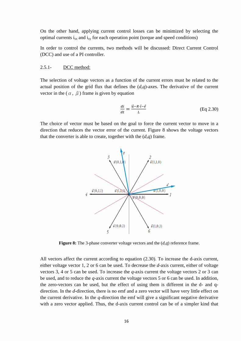
direction that reduces the vector error of the current. Figure 8 shows the voltage vectors

that the converter is able to create, together with the (d,q) frame.

Figure 8: The 3-phase converter voltage vectors and the (d,q) reference frame.

All vectors affect the current according to equation (2.30). To increase the d-axis current,

either voltage vector 1, 2 or 6 can be used. To decrease the d-axis current, either of voltage

vectors 3, 4 or 5 can be used. To increase the q-axis current the voltage vectors 2 or 3 can

be used, and to reduce the q-axis current the voltage vectors 5 or 6 can be used. In addition,

the zero-vectors can be used, but the effect of using them is different in the d- and q-

direction. In the d-direction, there is no emf and a zero vector will have very little effect on

the current derivative. In the q-direction the emf will give a significant negative derivative

with a zero vector applied. Thus, the d-axis current control can be of a simpler kind that

17

only uses active vectors in either direction to control the current, whereas the q-axis current

controller benefit from using zero vectors and thus must be more advanced.

The tolerance band used in the d-axis is the one presented on Figure 9 left. The tolerance

band used in the q-axis is the one presented on Figure 9 right.

Figure 9: The tolerance bands used in the 3 phases DCC.

Note that the entity “rest” in Figure 9 implies the use of a zero vector.

2.5.2- PI control method

A discrete-time, dead-beat PI-controller is designed for each current component based on

voltage expressions

(Eq 2.31)

(Eq 2.32)

The output from the controller is two voltage references, one in d- and one in q-direction.

The first step is to use backward Euler approximation for the current derivatives. This

gives

(Eq 2.33)

(Eq 2.34)

Furthermore, it is assumed that the currents can be approximated with their average values,

in the particular sampling interval

(Eq 2.35)

(Eq 2.36)

18

It is also assumed that the grid voltage does not change between two samples.

Consequently,

(Eq 2.37)

(Eq 2.38)

with the electromagnetic force in the d direction in the sample instant k and the

electromagnetic force in the q direction in the sample instant k.

This gives the following result

(Eq 2.39)

(Eq 2.40)

Since a dead-beat controller is considered, it is assumed that

(Eq 2.41)

(Eq 2.42)

giving

(Eq 2.43)

(Eq 2.44)

This gives a P-controller according to

(Eq 2.45)

(Eq 2.46)

The resistive voltage drop term can be interpreted as an integral part assuming that the

current equals the sum of all the previous current errors, i.e.

(Eq 2.47)

(Eq 2.48)

19

This gives a PI controller

(Eq 2.49)

(Eq 2.50)

where

(Eq 2.51)

(Eq 2.52)

with K the proportional constant and Ti the integral constant.

Using the assumptions

(Eq 2.53)

(Eq 2.54)

the equations will be

(Eq 2.55)

(Eq 2.56)

Where

with K the proportional constant, Ti the integral constant and Kc the feed forward constant.

20

3. - Test method: Description

3.1 - Description

The objective of this master thesis is to characterize a certain electrical machine (in this

case a PMSM), obtaining its torque, flux and efficiency maps for different operation points

of the machine (combinations of the isx and isy currents).

However, instead of coupling a speed and torque transducer to the test motor and run it

against a braking motor, the proposed method consists on accelerating the test motor back

and forth applying different current set-points. Assuming that the motor currents, voltages,

and speed can be measured accurately (with a sampling frequency high enough) and

provided that the inertia of the rotary part is known, the torque, flux and efficiency maps

can be determined.

The stator windings are fed by a three-phase current which are obtained from the DC

voltage source after passing through the inverter.

The operational path followed is described below:

1) A reference value of isx is fixed

2) Since the motor shaft spins freely, a speed controller (in this case a PI controller) is

needed, to guarantee that maximum speed is not exceeded. The output of the speed

controller is the reference value for isy.. The speed controller is implemented with a

high gain and the reference output isy is saturated at a set value, in order to have

constant values for isx and isy for a sufficient amount of time.

3) Then, when the difference between the reference speed and the measured speed is

large enough, the speed controller output will be saturated at the chosen isy value,

and isx and isy will be constant until the reference speed is met. Adding a flywheel

to the experiment will increase the time needed to reach the reference speed, hence

increasing the number of samples for a particular current set-point, easing the post

processing of the results and increasing the reliability of the results

4) Measuring the rotor acceleration, currents and voltages while isx and isy are

constant, torque, flux and estimative values of looses could be calculated for that

combination of currents.

5) This operation path would be repeated for different values of isx and different

values of the saturation for the speed controller (isy), scanning the whole operation

region of the motor.

The experiment is conducted for a certain set of isx and isy current combinations limited by

isx,max and isy,max. The x-axis current reference isx varies from 0 to -isx,max, while isy varies

from -isy,max to +isy,max. For each current set-point, the motor starts at standstill, it runs until

it reaches the reference speed and then brakes down to standstill again. This gives

acceleration and braking information for each operational point (this is one of the

contributions of this thesis, since previously only the acceleration was measured). As it

21

could be expected, for positives values of isy the rotor spins in one direction, and for

negatives values of isy it runs in the opposite direction. The value isy=0 is not considered,

because it gives no rotation.

3.2 - Simulation model

In order to demonstrate the validity of the method a simulation model is created. Using this

model it would be proven that the proposed method gives good results and the motor can

be characterized just measuring the currents, the voltages and the position/speed of the

rotor.

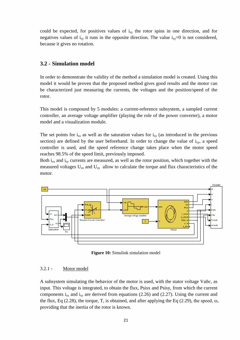
This model is compound by 5 modules: a current-reference subsystem, a sampled current

controller, an average voltage amplifier (playing the role of the power converter), a motor

model and a visualization module.

The set points for isx as well as the saturation values for isy (as introduced in the previous

section) are defined by the user beforehand. In order to change the value of isy, a speed

controller is used, and the speed reference change takes place when the motor speed

reaches 98.5% of the speed limit, previously imposed.

Both isx and isy currents are measured, as well as the rotor position, which together with the

measured voltages Usx and Usy allow to calculate the torque and flux characteristics of the

motor.

Figure 10: Simulink simulation model

3.2.1 - Motor model

A subsystem simulating the behavior of the motor is used, with the stator voltage Vabc, as

input. This voltage is integrated, to obtain the flux, Psisx and Psisy, from which the current

components isx and isy are derived from equations (2.26) and (2.27). Using the current and

the flux, Eq (2.28), the torque, T, is obtained, and after applying the Eq (2.29), the speed, ω,

providing that the inertia of the rotor is known.

22

Figure 11: Motor model

The parameters used to define the motor behavior are:

- Flux from rotor magnets linking the stator windings (Psim)

- Number of poles, p

- Stator resistance, Rs

- X-axis stator inductance, Lsx

- Y-axis stator inductance, Lsy

- Inertia, J

3.2.2 - PI controller model

According to the control strategy defined in the previous section, the voltages Vabc are the

output of the PI current controller, calculated from the current set point (isx and isy

references), the actual isx and isy currents and the rotor position given by the motor

simulation model.

The parameters used for this PI controller subsystem are:

- Controller gain, K

- Integral Time constant, Ti

- Sampling time, Ts

- Max output signal, Udc

23

According to the theory presented in section 2.5, the controller gain is calculated as

[(Lsx/Ts+Rs/2) (Lsy/Ts+Rs/2)]' for x and y axis respectively, and the integral time

constant is calculated as [(Lsx/Rs+Ts/2) (Lsy/Rs+Ts/2)]' for x and y axis respectively.

3.2.3 - Currents reference subsystem

A subsystem is created in order to generate the reference signals isx* and isy*.

Figure 12: Currents reference subsystem model

In this subsystem, the inputs are the electrical speed, ωel, and the measured currents isx and

isy. The speed signal together with the speed reference is fed to a PI controller, where the

torque is obtained. Then, from Eq (2.28), with Lsx = Lsy, T = Psim·isy, isy is easily obtained

(note that the value of Psim is included in the PI controller and therefore it is not visible in

Figure 12). As mentioned in the previous section, if this isy value is bigger than the user

defined saturation value corresponding to the current iteration of the method Isy, it will be

saturated to Isy.

Parameters used in this subsystem are:

- Speed controller gain, Kpw

- Speed controller integral time constant, Tiw

- Speed reference, W_ref

- Maximum current, Imax

24

3.3 - Postprocessing

All the data obtained from the simulations and/or the experimental tests is later processed

in Matlab, in order to obtain the most relevant characteristics of the motor such as the

torque and flux maps.

3.3.1 - Torque map

Once we have the results for speed, torque can be calculated, using.

(Eq 3.1)

The derivative of the speed is computed using the center difference method:

(Eq 3.2)

After computing the values of dw/dt for each sampling interval, the mean value is

calculated, and this mean value is used to calculate the average torque for each

combination of (isx , isy).

3.3.2 - Flux map

From the voltages usx and usy and knowing the ψm of the motor, the stator flux can be

calculated from:

(Eq 3.3)

(Eq 3.4)

Where:

(Eq 3.5)

(Eq 3.6)

It is worth noticing that the voltages usx and usy are not easy variables to measure,

especially if the motor is fed with a Pulse-Width Modulated voltage. New data acquisition

devices like the ones used in this thesis, make possible the accurate computation of usx and

usy through a high frequency sampling of the motor voltages. However, in those cases

where usx and usy may not be measurable, they can be estimated using the output of the

current PI controllers.

25

3.3.3 - Losses

Total motor losses are calculated as the difference between the input electrical power and

the output mechanical power.

Electrical power is obtained from:

(Eq 3.7)

And mechanical power is obtained applying:

(Eq 3.8)

with T the torque, f the electrical rotational frequency and np the number of poles.

Motor losses can be classified into mechanical, magnetic or electrical losses. Mechanical

losses are due to friction in different parts of the machine, and comprise bearing losses and

windage losses (friction with the air surrounding the rotor). Magnetic losses are due to

hysteresis and eddy currents and appear mostly in the lamination plates of the motor and

the permanent magnets. Electrical losses (also called copper losses), are mostly due to the

Joule effect in the current conductors and the time harmonics produced by the switching of

the power electronics applied in the control of the motor. Classification of different losses

is not discussed in this thesis.

3.4 - Lab setup description: Hardware and Software

The hardware used in this master thesis is:

- Inverter (transistors and drivers)

o Inverter SKIIP SEMIKRON 513GD172-3 DUL V3: 1700 V, 500 A

Semidrivers SKIC 6001

- Acquisition system (signal conditioning boards)

o National Instruments cRIO

Module NI9223: 4-Channel, 1 MS/s, 16-Bit Simultaneous Analog Input

Module NI9215: 4-Channel, 100 kS/s/ch, 16-bit, ±10 V Analog Input

Module NI9205: 32-Ch, ±200 mV to ±10 V, 16-Bit, 250 kS/s Analog Input

Module NI9263: 4-Channel, 100 kS/s, 16-bit, ±10 V, Analog Output

Module NI9401: 8 Ch, 5 V/TTL High-Speed Bidirectional Digital

Module NI9402: 4 Ch LVTTL High-Speed Digital I/O

- Power supplies 5 V and 15 V

26

- Sensors (current/voltage/resolver)

o Currents probes LEM LT100-S

o Voltages probes Tektronix P5200 1/50

o Resolver Variable reluctance resolver Singlsyn (Tamagawa)

- Computer.

In this master thesis, National Instruments LabVIEW and Compact Rio (cRIO) is used for

the control of the motor and the acquisition of the data. Measured signals of currents,

voltages and rotor position, acquired thanks to the different probes and sensors are

introduced in the corresponding CompactRio module. This data is used to calculate the

reference voltages for the next sampling time. Besides, the data is sent to the computer

where it is logged in order to be postprocessed offline, when the experiment finishes. The

cRIO hardware is as well responsible to generate the switching signal for the IGBT.

Matlab (Mathworks) software is used for the simulations and the post processing of the

sampled signals. Both the LabVIEW and Matlab routines used were developed at the

Industrial Electrical Engineering and Automation department at LTH and have been

adapted to meet the experiment’s needs.

27

4. - Simulations results

Next the results obtained from the simulation of the test method are presented. In the

simulation, the tested motor is characterized by the parameters Lsx = Lsy = 0.003 H and =

0.16.

The values of isx and isy that have been taken into consideration are:

- isx is limited from -40A to 0A, divided into 8 steps of 5A each one.

- isy is limited from -40A to 40A, with steps of 5A, creating 16 values. isy=0A is not used.

For each value of isx, all values of isy are used, starting with 5A, followed by -5A, and after

that 10A, and so on, with last values of 40A and -40A. Once the value of isy returns to 5A, isx

changes to the next value. The values change in decreasing direction.

To obtain the maps, Matlab scripts have been created using the results from Simulink. These

scripts can be found in the Appendix (Torque maps simulation and flux maps simulations).

In the following figures, the maps resulting from the simulation are presented.

Figure 13: Torque obtained from simulation

28

Figure 14: Torque mesh obtained from simulation

Figure 15: Flux obtained from simulation

29

Figure 16: Flux mesh obtained from simulation

From these maps, the most relevant motor parameters such as inductances Lsx and Lsy, and

the permanent magnet flux can be calculated using a Matlab script (see validation script

in appendix). Results obtained from this script are:

Lsx Lsy

Set values 0.003 0.003 0.16

Calculated values 0.003 0.003 0.16

Table 3: Comparative values of Lsx, Lsy and Psim

30

5. - Experimental results

In this section the experimental results obtained in the course of this thesis are presented. In

order to validate these results, they are compared to simulation results obtained from the

Finite Elements model of the motor and also to the motor characteristics obtained from

previous experiments using traditional methods.

The speed reference is set to different values depending on the isx reference, since the

maximum speed that can reach the motor for low values of isx is not the same as for higher

values due to the field weakening effect. The actual speed limits (in terms of electrical

frequency) are 150 Hz for 0 A, 170 Hz for -5 A, 180 Hz for -10 and -15 A, 190 Hz for -20 A

and 200 Hz for the rest of isx reference values.

In order to improve the results, a flywheel could be coupled to the rotor to increase the time

needed to reach the reference speed, hence increasing the number of samples for a particular

current set-point, easing the post processing of the results and increasing the reliability of the

results.

5.1 - Estimation of the rotating mass inertia

As shown in Eq. 3.1 in order to compute the torque values, we need to know the inertia of

the rotary mass and the time derivative of the rotational speed of the motor. The speed of

the motor is sampled with sufficient sampling rate, and therefore the derivative can be

easily calculated (Eq 3.2). The inertia of the rotating mass however has to be estimated

from the geometry and the material properties of the mass.

The rotating mass consists of the rotor laminations and magnets, the rotor shaft and an

extra flywheel attached to it in order to increase the total inertia thus obtaining more

accurate results.

The rotor laminations and magnets geometry is presented in figure 17, assuming a

homogenous density with a value of 7850 kg/m3.

The rotor inertia is calculated as the addition of three cylinders, the main one in the center

and a small one in each side of this, as it can be seen in the figure 17. The equation to

calculate the inertia moment is:

(Eq. 5.1)

being ro1 and ro2 the external radius of the main and secondary cylinders respectively and

ri the internal radius of both of them and l1 the length of the main cylinder and l2 the length

of each of the secondary cylinders.

31

Figure 17: Rotor

In figure 18 the rotor shaft is presented. A homogenous density with value of 7850 kg/m3 is

assumed. The inertia moment for the shaft is calculated as:

(Eq. 5.2)

with the radius of the j section of the shaft and the length of the j section of the shaft.

Figure 18: Rotor shaft

The flywheel used in the realization of this Thesis has a mass of 5.65 kg, with a cylindric-

conic-cylindrical shape as it is shown in figure 19.

Knowing the density and the dimensions of the flywheel, the inertia moment is calculated

as:

(Eq 5.3)

(Eq 5.4)

32

being ro the external radius of the cylinder and ro1 and ro2 the base and top respectively

radius of the conical frustum and ri the internal radius of both of them.

Figure 19: Flywheel of 5.65 kg

Final inertia moment is calculated as the addition of the inertia moment of the cylinders

plus the conical frustum.

The density was calculated assuming that it is homogeneous for the entire flywheel and it

has a value of 8004 kg/m3.

Inertia values (kg·m2)

Rotor laminations and magnets 0.02651600

Rotor shaft 0.00016217

Flywheel big cylinder 0.02610000

Flywheel cone 0.00085017

Flywheel small cylinder 0.00069714

Flywheel 0.02770000

Total inertia 0.05380400

Table 4: Inertia values

33

5.2 - Experimental results

The following figures present the results when the motor is coupled to a flywheel of 5.65

kg.

Figure 20: Experimental torque mesh

Figure 21: Experimental torque map

34

Figure 22: Experimental stator flux linkage in the x-axis

Figure 23: Experimental stator flux linkage in the y-axis

35

Figure 24: Experimental stator flux linkage map

Figure 25: Experimental stator flux linkage mesh

36

6. - Comparative study of the results

In this section experimental results are compared with the results of the Finite Element

simulations of the tested motor and with the verified motor characteristics, obtained from

previous experiments using traditional methods.

6.1 - Experimental vs. FE simulations

For the output torque, the comparative map is:

Red values are for simulation results and blue values are for experimental results.

Figure 26: Experimental vs. simulation torque

In the next figure, the simulation results correspond to the mesh and the experimental

values are represented by a surface, smaller than the simulation mesh.

37

Figure 27: Experimental vs. simulation torque

For the stator flux linkage, the comparative map is:

Red values are used for simulation results and blue values for experimental results.

Figure 28: Experimental vs. simulation flux

38

In the next figure, the simulations results are represented in a mesh and experimental

results are represented in a surface.

Figure 29: Experimental vs. simulation flux mesh

6.2 - Experimental vs. verified motor characteristics

For the output torque, the comparative map is:

Red values are used for verified motor characteristics and blue ones for the experimental

results obtained in this thesis.

Figure 30: Experimental vs. verified torque

39

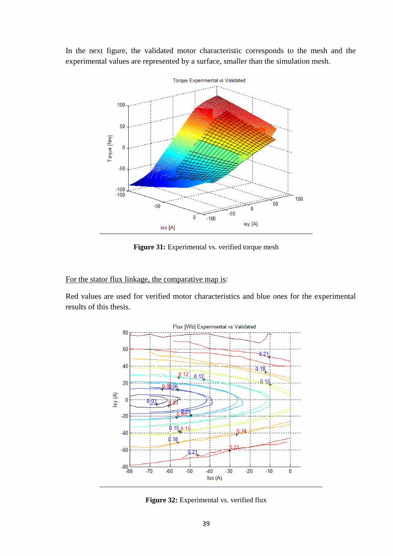
In the next figure, the validated motor characteristic corresponds to the mesh and the

experimental values are represented by a surface, smaller than the simulation mesh.

Figure 31: Experimental vs. verified torque mesh

For the stator flux linkage, the comparative map is:

Red values are used for verified motor characteristics and blue ones for the experimental

results of this thesis.

Figure 32: Experimental vs. verified flux

40

Figure 33: Experimental vs. verified flux mesh

41

7. - Conclusions

7.1 - Simulations

As a first step during the course of this thesis, simulations are conducted in order to verify

the first assumptions on how the experiments should be carried out and which variables

should be measured. A simulation model is developed in Simulink, and several simulations

are conducted, showing that the assumptions were correct: measuring currents, voltages

and position/speed of the motor fast enough and with enough accuracy, the torque and flux

linkage maps for the characterization of the motor can be obtained.

In these simulations, certain motor parameters are predefined, namely the stator resistance

and x and y inductances and the magnetization flux. After simulating the whole

experimental sequence, the logged data is processed, obtaining the torque and flux maps,

from which the values of the previous motor parameters are calculated.

The results presented in section 4 show that the calculated parameters match the predefined

ones, and therefore, the method is valid (at least in the “ideal” simulated world).

7.2 - Simulations vs. experimental results

It can be observed that the torque results obtained from the FE simulations and the

proposed method are really close for low values of isy. For high values of isy, iso-torque

lines from experimental results are located slightly below those from the simulations

results, meaning that a lower current is needed to achieve the same torque level. This can

be explained by the assumption of an elevated magnet temperature (80 deg C) made in the

FE simulation model. However, the error is not significant and both maps present similar

shape and slope.

In the stator flux linkage comparative, it can be observed that results are quite similar for

all values of isx and isy. For high values of isx, a small deviation occurs in the slope of

values of the flux linkage and according to the experimental results, more negative current

is needed in the x-axis to demagnetize the machine. This could also be a consequence of

the assumption made in the magnet temperature in the simulations. It is worth noticing that

flux values for isy=[-10,10] are obtained by interpolation of the experimental results.

7.3 - Experimental vs. verified motor characteristics

When comparing the torque obtained in the experiment to the existing motor

characteristics, the differences are minimal, and it can be observed that the new curves are

smoother than those obtained from previous works due to the high sampling speed and

42

improved accuracy of the new measurement system. The fact that the whole experiment

sequence is carried out within a few minutes time, avoids the raise in the motor

temperature that occurs with the much slower traditional methods, and therefore the results

are not affected by the changing conditions during the execution of the experiment.

In the stator flux linkage case, it can be seen that for higher values of the flux linkage, the

curves are slightly moved to upper values of isy. However, the difference is also

insignificant and both the new experimental map and the validated one highly match. Here,

the curves are also smoother than the previous ones. It is worth noticing that flux values for

isy= [-10,10] are obtained by interpolation of the experimental results.

7.4 - Note on the experimentally obtained motor characteristics

Besides the aforementioned difference between the motor characteristics obtained with the

presented novel method when compared to more traditional experiments, and which can be

explained by the difference in the duration of the tests and its implications mostly in the

temperature of the magnets and the windings, there is another difference which is worth

noticing.

When looking at Figure 30, it can be seen that while the effect of a lower temperature

development in the novel method is clearly seen for the positive isy half plane, this effect is

not present in the lowest half plane. The reason for this is that while in the curves obtained

with traditional testing methods (so called validated motor characteristics) a negative isy is

applied when the motor has a positive speed (i.e. trying to brake the motor, and therefore

operating as a generator), in the presented method, when a negative isy is applied, the rotor

starts spinning in the negative direction, and therefore, the machine is still acting as a

motor.

When operating as a generator (applying a torque of the opposite sign of the speed) the

losses in the motor contribute to this effect, and therefore, a lower value of the current is

needed to achieve the same absolute value of the torque than that one needed in motor

operation. This can be noticed in Figure 27, where for negative values of isy in the

validated motor characteristics, the difference due to the increased temperature is

compensated with the generation effect, and both methods show nearly identical results.

7.5 - Final conclusion

In this thesis, a novel method for characterizing electric motors is introduced. Compared to

the traditional test methods, the proposed method presents a number of advantages:

- There is no need for either a braking load or a torque transducer

- The whole test sequence is completely automated as well as the postprocessing of the

experimental results

43

- The machine is tested within a few minutes time, avoiding the drift in the results

originated from the variation of temperature and other conditions.

With the results presented in the previous sections, it has been proven that the method

presented and studied in this thesis is a valid method to characterize electric motors.

44

8. - Further development of the method

Due to the limited time available for the realization of the thesis, there are a few things that

could not be completed, and they are presented here as suggestions for the further

development of the method.

a) Loss separation: Although it was not graphically presented in the thesis, motor

efficiency is calculated as the ratio between output (mechanical) power and input

(electric) power. However, in order to improve the efficiency of the motor it is

interesting to know where the losses are generated in the machine. Thus, the presented

method will benefit from the implementation of a loss separation algorithm that helps

to evaluate the distribution of losses within the motor.

b) Current control: During the execution of the experiments, the current controllers

behaved in an unexpected way when operating the machine at high speeds (near the

maximum voltage limitation of the inverter). Therefore, all the experiments conducted

had a speed limitation of 3000 rpm (200 Hz for an 8-pole machine). A more advanced

current control strategy will allow for higher speeds, which could lead to more

accurate flux maps.

c) Accuracy assessment: In this thesis the validity of the method has been proven.

However, no quantitative evaluation of the accuracy of the method has been presented.

In order to determine the applicability of the method in different situations (f. ex. for

certification applications, where high accuracy motor maps are required) the method

should be applied to a well known reference machine, and the results properly

analyzed taking into account any possible deviations (the accuracy of the different

transducers, calibration errors, temperature drifts, etc.).

45

9. - References

Chapter 1:

- Power Electronics: Devices, Converters, Control and Applications by Mats Alaküla

and Per Karlsson.

- www.wikipedia.org

Chapter 2:


and Per Karlsson.

- www.wikipedia.org

- http://earlyelectric.com/

- http://www.ece.msstate.edu/~donohoe/ece3414synchronous_machines.pdf

- http://www.magnetsales.com

- http://www.intemag.com

- http://www.iieom.org/ieom2011/pdfs/IEOM193.pdf

Chapter 3:


and Per Karlsson.

- Energy efficiency in motor driven systems, by Francesco Parasiliti,Paolo Bertoldi

- http://www.engineeringtoolbox.com/electrical-motor-efficiency-d_655.html

http://www.wikipedia.org/

http://www.wikipedia.org/

http://earlyelectric.com/

http://www.ece.msstate.edu/~donohoe/ece3414synchronous_machines.pdf

http://www.magnetsales.com/Neo/Neo1.htm

http://www.intemag.com/

http://www.iieom.org/ieom2011/pdfs/IEOM193.pdf

http://www.engineeringtoolbox.com/electrical-motor-efficiency-d_655.html

46

10. - Appendix: Developed software

10.1- Torque maps simulation

%% Calculation of Torque using T=J·dw/dt

% Calculation of dw/dt and comparative methods of calculation for the

torque

time0 = cputime; % Initialization for calculating the time of

calculate dw/dt using stretches

for ii = 1:500 dw1(ii) = ((w_el(ii+150,2)-w_el(ii+149,2))/(w_el(ii+150,1)-

w_el(ii+149,1))); dw2(ii) = ((w_el(ii+651,2)-w_el(ii+650,2))/(w_el(ii+651,1)-






w_el(ii+3150,1))); end

w1_avg_1 = mean(dw1) % Part 1 w1_avg_2 = mean(dw2) % Part 2 w1_avg_3 = mean(dw3) % Part 3 w1_avg_4 = mean(dw4) % Part 4 w1_avg_5 = mean(dw5) % Part 5 w1_avg_6 = mean(dw6) % Part 6 w1_avg_7 = mean(dw7) % Part 7

w1_avg_parts =

(w1_avg_1+w1_avg_2+w1_avg_3+w1_avg_4+w1_avg_5+w1_avg_6+w1_avg_7)/7 %

Average parts 1 to 7

time1 = cputime-time0 % Calculation time for calculate dw/dt using

stretches

time2_1 = cputime; % Initialization for calculating the time of

calculate dw/dt using backward difference method

for iii = 1:3800 dw(iii) = ((w_el(iii+Pos_w1,2)-w_el(iii+Pos_w1-

1,2))/(w_el(iii+Pos_w1,1)-w_el(iii+Pos_w1-1,1))); end

w1_av = mean(dw) % Using all data, with backward difference

method for calculate the differential

47

time2 = cputime-time2_1; % Calculation time for calculate dw/dt using

backward difference method

time3_1 = cputime; % Initialization for calculating the time of

calculate dw/dt using central difference method

for jjj = 1:3799 dwc(jjj) = ((w_el(jjj+Pos_w1,2)-w_el(jjj+Pos_w1-

2,2))/(2*(w_el(jjj+Pos_w1,1)-w_el(jjj+Pos_w1-1,1)))); end

w1_avg_c = mean(dwc) % Using central difference method for calculate

the differential

time3 = cputime-time3_1; % Calculation time for calculate dw/dt using

central difference method

% Torque calculation

T1_1 = J*w1_avg_1 T1_2 = J*w1_avg_2 T1_3 = J*w1_avg_3 T1_4 = J*w1_avg_4 T1_5 = J*w1_avg_5 T1_6 = J*w1_avg_6 T1_7 = J*w1_avg_7

T1_avg = J*w1_avg_parts

T1 = J*w1_av T1_c = J*w1_avg_c

Results_1(3,1) = w1_avg_c; Results_1(4,1) = T1_c;

time1 time2 time3

figure (1) plot (dw,'r+'); hold on plot (dwc,'bx'); title('dw/dt using backwards and central difference '); xlabel('Position'); ylabel('dw/dt');

figure (2) plot (dw1,'r-') hold on plot (dw2,'b-') plot (dw3,'g-') plot (dw4,'k-') plot (dw5,'r.') plot (dw6,'b.') plot (dw7,'g.') title('dw/dt using stretches'); xlabel('Position'); ylabel('dw/dt');

48

% Calculation of dw/dt and T for all values, using central difference

method

clear dw1_c;

for jj=0:8 if jj==0

for ii = 1:3790 dw1_c(ii) = ((w_el(ii+(Pos_w1+jj*Gap),2)-

w_el(ii+(Pos_w1+jj*Gap-2),2))/(2*(w_el(ii+(Pos_w1+jj*Gap),1)-

w_el(ii+(Pos_w1+jj*Gap-1),1)))); end else for ii = 1:7400 dw1_c(ii) = ((w_el(ii+(Pos_w1+jj*Gap-3900),2)-

w_el(ii+(Pos_w1+jj*Gap-3900)-2,2))/(2*(w_el(ii+(Pos_w1+jj*Gap-3900),1)-

w_el(ii+(Pos_w1+jj*Gap-3900)-1,1)))); end end

w1_avg(jj+1) = mean(dw1_c); T1_avg(jj+1) = J*w1_avg(jj+1);

Results(3,1+16*jj) = w1_avg(jj+1); Results(4,1+16*jj) = T1_avg(jj+1);

clear dw2_c;

for ii = 1:7600 dw2_c(ii) = ((w_el(ii+Pos_w2+jj*Gap,2)-w_el(ii+Pos_w2+jj*Gap-

2,2))/(2*(w_el(ii+Pos_w2+jj*Gap,1)-w_el(ii+Pos_w2+jj*Gap-1,1)))); end



clear dw3_c;





clear dw4_c;

for ii = 1:3600

49

dw4_c(ii) = ((w_el(ii+Pos_w4+jj*Gap,2)-w_el(ii+Pos_w4+jj*Gap-




clear dw5_c;





clear dw6_c;





clear dw7_c;





clear dw8_c;




50


clear dw9_c;





clear dw10_c;





clear dw11_c;





clear dw12_c;





clear dw13_c;

51





clear dw14_c;





clear dw15_c;





clear dw16_c;




Results(3,16+16*jj) = w16_avg(jj+1); Results(4,16+16*jj) = T16_avg(jj+1); end

%% Torque values

for ii=0:8 for jj=1:16 T(ii+1,jj) = Results(4,16*ii+jj); end

52

end

10.2- Flux maps simulation

%% Obtention of Psis for Results matrix

% Index for speed, w, changes

inw_Psi = find((((Psis_wel(:,4))>=-240) & ((Psis_wel(:,4))<=240))); for ii=1:(length(inw_Psi)-1) if (inw_Psi(ii+1)-inw_Psi(ii))>1; inw_Psi_ch(ii)=inw_Psi(ii); end end

inw_Psi_val = find(inw_Psi_ch ~= 0);

for ii=0:(length(inw_Psi_val)) if ii==0 for jj=1:inw_Psi(inw_Psi_val(ii+1)); Psisx_rough(ii+1)=mean(Psis_wel(jj,2)); Psisy_rough(ii+1)=mean(Psis_wel(jj,3)); end elseif ii==length(inw_Psi_val) for jj=inw_Psi(inw_Psi_val(ii)+1):inw_Psi(length(inw_Psi)) Psisx_rough(ii+1)=mean(Psis_wel(jj,2)); Psisy_rough(ii+1)=mean(Psis_wel(jj,3)); end else for jj=inw_Psi(inw_Psi_val(ii)+1):inw_Psi(inw_Psi_val(ii+1)) Psisx_rough(ii+1)=mean(Psis_wel(jj,2)); Psisy_rough(ii+1)=mean(Psis_wel(jj,3)); end end end

Results(5,:) = Psisx_rough; Results(6,:) = Psisy_rough;

% Calculus of mesh of Psisx and Psisy

Psisx = Results(5,:); Psisy = Results(6,:);

Psi = sqrt(Psisx.^2+Psisy.^2);

for ii=0:8 for jj=1:16 Psi_mesh(ii+1,jj) = Psi(16*ii+jj); Psisx_mesh(ii+1,jj) = Psisx(16*ii+jj); Psisy_mesh(ii+1,jj) = Psisy(16*ii+jj); end end

10.3- Postprocessing for torque and flux maps

53

%% Postprocessing of the data for Simulations of a PMSM

% Isx and Isy

for ii=0:8 isx(ii+1) = Results(1,1+ii*16); for j=1:8 isy(2*j-1) = Results (2,ii*16+2*j-1); isy(2*j) = Results (2,ii*16+2*j); end end

% Torque

for ii=0:8 for jj=1:16 T(ii+1,jj) = Results(4,16*ii+jj); end end

% Flux


Psi = sqrt(Psisx.^2+Psisy.^2);

for ii=0:8 for jj=1:16 Psi_mesh(ii+1,jj) = Psi(16*ii+jj); end end

% Figures

[ixx,iyy] = meshgrid(-40:0,-40:40);

T_int = griddata(isx,isy,T',ixx,iyy,'cubic'); figure (3) [C,h] =contour(ixx,iyy,T_int); title('Torque'); xlabel('Isx (A)'); ylabel('Isy (A)'); clabel(C,'HorizontalAlignment','center');

figure (4) mesh(ixx,iyy,T_int) title('Torque'); xlabel('Isx (A)'); ylabel('Isy (A)');

Psi_int=griddata(isx,isy,Psi_mesh',ixx,iyy,'cubic'); figure (5) [C1,h1] = contour(ixx,iyy,Psi_int); title('Flux (Psi)'); xlabel('Isx (A)'); ylabel('Isy (A)'); clabel(C1,'HorizontalAlignment','center');

54

figure (6) mesh(ixx,iyy,Psi_int) title('Flux (Psi)'); xlabel('Isx (A)'); ylabel('Isy (A)');

10.4- Validation script (Lsx, Lsy and Psim)

% Validation: Obtention of Psim, Lsx and Lsy


IsxVal = 4; IsyVal = 15;

for ii=0:8 isx(ii+1) = Results(1,1+ii*16); PsisxVal(ii+1) = Psisx(IsyVal+16*ii);

for j=1:8 isy(2*j-1) = Results (2,ii*16+2*j-1); isy(2*j) = Results (2,ii*16+2*j); end end

PsisyVal = Psisy((IsxVal-1)*16+1:IsxVal*16);

plot(isx,PsisxVal) CoefValX = polyfit(isx,PsisxVal,1); CoefValY = polyfit(isy,PsisyVal,1);

PsimVal = CoefValX(2) LsxVal = CoefValX(1) LsyVal = CoefValY(1)

dynamic braking industrial electrical engineering and ... document/5292_full... · division of...

Documents