dynamic classification of escape time sierpinski curve julia sets dynamics of the family of complex...
Post on 19-Dec-2015
213 views
TRANSCRIPT

Dynamic Classification of Escape TimeSierpinski Curve Julia Sets
Dynamics of the family of complex maps
Paul BlanchardToni GarijoMatt HolzerU. HoomiforgotDan LookSebastian Marotta
with:
€
Fλ (z) = zn +λ
zn
Mark MorabitoMonica Moreno RochaKevin PilgrimElizabeth RussellYakov ShapiroDavid Uminsky
, n > 1

A Sierpinski curve is any planar set that is homeomorphic to the Sierpinski carpet fractal.
QuickTime™ and aTIFF (LZW) decompressor
are needed to see this picture.
The Sierpinski Carpet
Sierpinski Curve

QuickTime™ and aTIFF (LZW) decompressor
are needed to see this picture.
The Sierpinski Carpet
Topological Characterization
Any planar set that is:
1. compact2. connected3. locally connected4. nowhere dense5. any two complementary domains are bounded by simple closed curves that are pairwise disjoint
is a Sierpinski curve.

Any planar, one-dimensional, compact, connected set can be homeomorphically embedded in a Sierpinski curve.
More importantly....
A Sierpinski curve is a universal plane continuum:
For example....

QuickTime™ and aTIFF (LZW) decompressor
are needed to see this picture.
This set

QuickTime™ and aTIFF (LZW) decompressor
are needed to see this picture.
This set
QuickTime™ and aTIFF (LZW) decompressor
are needed to see this picture.
can be embedded inside

QuickTime™ and aTIFF (LZW) decompressor
are needed to see this picture.
This set
QuickTime™ and aTIFF (LZW) decompressor
are needed to see this picture.
can be embedded inside
Moreover, Sierpinski curves occur all the time as Julia sets.

Dynamics of
complex and
€
Fλ (z) = z n +λ
z n
€
λ,z
€
n ≥ 2
A rational map of degree 2n.
Also a “singular perturbation” of zn.

QuickTime™ and aTIFF (LZW) decompressor
are needed to see this picture.
€
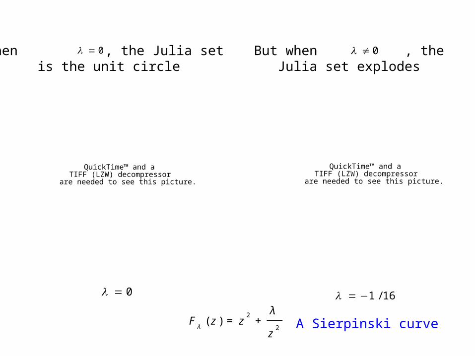
λ = 0
€
Fλ
( z ) = z2
+λ
z2
When , the Julia set is the unit circle
€
λ = 0

QuickTime™ and aTIFF (LZW) decompressor
are needed to see this picture.
€
λ = 0
€
Fλ
( z ) = z2
+λ
z2
€
λ ≠ 0
€
λ = −1 / 16
QuickTime™ and aTIFF (LZW) decompressor
are needed to see this picture.
But when , theJulia set explodes
When , the Julia set is the unit circle
€
λ = 0
QuickTime™ and aTIFF (LZW) decompressor
are needed to see this picture.
€
λ = 0
€
Fλ
( z ) = z2
+λ
z2
€
λ ≠ 0
€
λ = −1 / 16
QuickTime™ and aTIFF (LZW) decompressor
are needed to see this picture.
But when , theJulia set explodes
A Sierpinski curve
When , the Julia set is the unit circle
€
λ = 0

QuickTime™ and aTIFF (LZW) decompressor
are needed to see this picture.
€
λ = 0
€
Fλ
( z ) = z2
+λ
z2
€
λ ≠ 0But when , theJulia set explodes
€
λ = −0 . 01
Another Sierpinski curve
QuickTime™ and aTIFF (LZW) decompressor
are needed to see this picture.
When , the Julia set is the unit circle
€
λ = 0

QuickTime™ and aTIFF (LZW) decompressor
are needed to see this picture.
€
λ = 0
€
Fλ
( z ) = z2
+λ
z2
€
λ ≠ 0But when , theJulia set explodes
€
λ = −0 . 2
Also a Sierpinski curve
QuickTime™ and aTIFF (LZW) decompressor
are needed to see this picture.
When , the Julia set is the unit circle
€
λ = 0
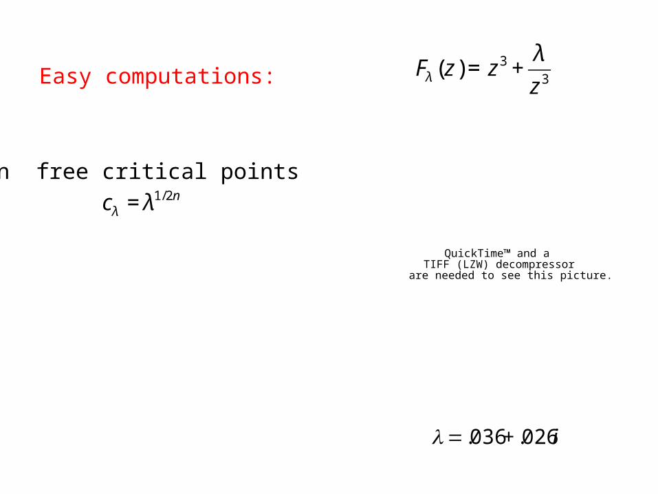
Easy computations:
QuickTime™ and aTIFF (LZW) decompressor
are needed to see this picture.
€
Fλ (z ) = z 3 +λ
z 3
€
λ=.036+.026i
2n free critical points
€
cλ = λ1/2n

Easy computations:
QuickTime™ and aTIFF (LZW) decompressor
are needed to see this picture.
€
λ=.036+.026i
2n free critical points
€
cλ = λ1/2n€
Fλ (z ) = z 3 +λ
z 3

Easy computations:
QuickTime™ and aTIFF (LZW) decompressor
are needed to see this picture.
€
λ=.036+.026i
2n free critical points
€
cλ = λ1/2n
Only 2 critical values
€
vλ = ±2 λ
€
Fλ (z ) = z 3 +λ
z 3

Easy computations:
QuickTime™ and aTIFF (LZW) decompressor
are needed to see this picture.
€
λ=.036+.026i
2n free critical points
€
cλ = λ1/2n
Only 2 critical values
€
vλ = ±2 λ
€
Fλ (z ) = z 3 +λ
z 3

Easy computations:
QuickTime™ and aTIFF (LZW) decompressor
are needed to see this picture.
€
λ=.036+.026i
2n free critical points
€
cλ = λ1/2n
Only 2 critical values
€
vλ = ±2 λ
€
Fλ (z ) = z 3 +λ
z 3

Easy computations:
€
λ=.036+.026i
2n free critical points
€
cλ = λ1/2n
Only 2 critical values
€
vλ = ±2 λ
But really only 1 freecritical orbit since
the map is symmetricunder
€
Fλ (z ) = z 3 +λ
z 3
QuickTime™ and aTIFF (LZW) decompressor
are needed to see this picture.
€
z → −z

Easy computations:
QuickTime™ and aTIFF (LZW) decompressor
are needed to see this picture.
€
λ=.036+.026i
is superattracting, so have immediate basin Bmapped n-to-1 to itself.
€
∞ B€
Fλ (z ) = z 3 +λ
z 3

Easy computations:
QuickTime™ and aTIFF (LZW) decompressor
are needed to see this picture.
€
λ=.036+.026i
is superattracting, so have immediate basin Bmapped n-to-1 to itself.
B
T
€
Fλ (z ) = z 3 +λ
z 3
€
∞
0 is a pole, so havetrap door T mapped
n-to-1 to B.

Easy computations:
QuickTime™ and aTIFF (LZW) decompressor
are needed to see this picture.
€
λ=.036+.026i
is superattracting, so have immediate basin Bmapped n-to-1 to itself.
B
T
€
Fλ (z ) = z 3 +λ
z 3
€
∞
So any orbit that eventuallyenters B must do so by
passing through T.
0 is a pole, so havetrap door T mapped
n-to-1 to B.

The Escape Trichotomy
There are three distinct ways the critical orbit can enter B:

The Escape Trichotomy
€
vλ∈
€
J ( Fλ
)
€
⇒B is a Cantor set
There are three distinct ways the critical orbit can enter B:

The Escape Trichotomy
€
vλ∈
€
J ( Fλ
)
€
⇒B is a Cantor set
T
€
vλ∈ is a Cantor set of
simple closed curves
€
J ( Fλ
)
There are three distinct ways the critical orbit can enter B:
(this case does not occur if n = 2)
€
⇒
(McMullen)

The Escape Trichotomy
€
vλ∈
€
J ( Fλ
)
€
⇒B is a Cantor set
T
€
vλ∈ is a Cantor set of
simple closed curves
€
J ( Fλ
)
€
Fλ
k(v
λ) ∈ T
€
J ( Fλ
) is a Sierpinski curve
There are three distinct ways the critical orbit can enter B:
(this case does not occur if n = 2)
€
⇒
€
⇒
(McMullen)

QuickTime™ and aTIFF (LZW) decompressor
are needed to see this picture.
€
vλ∈
€
J ( Fλ
)
€
⇒B is a Cantor set
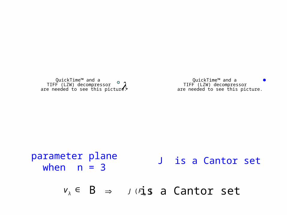
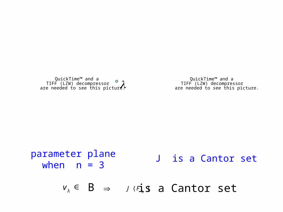
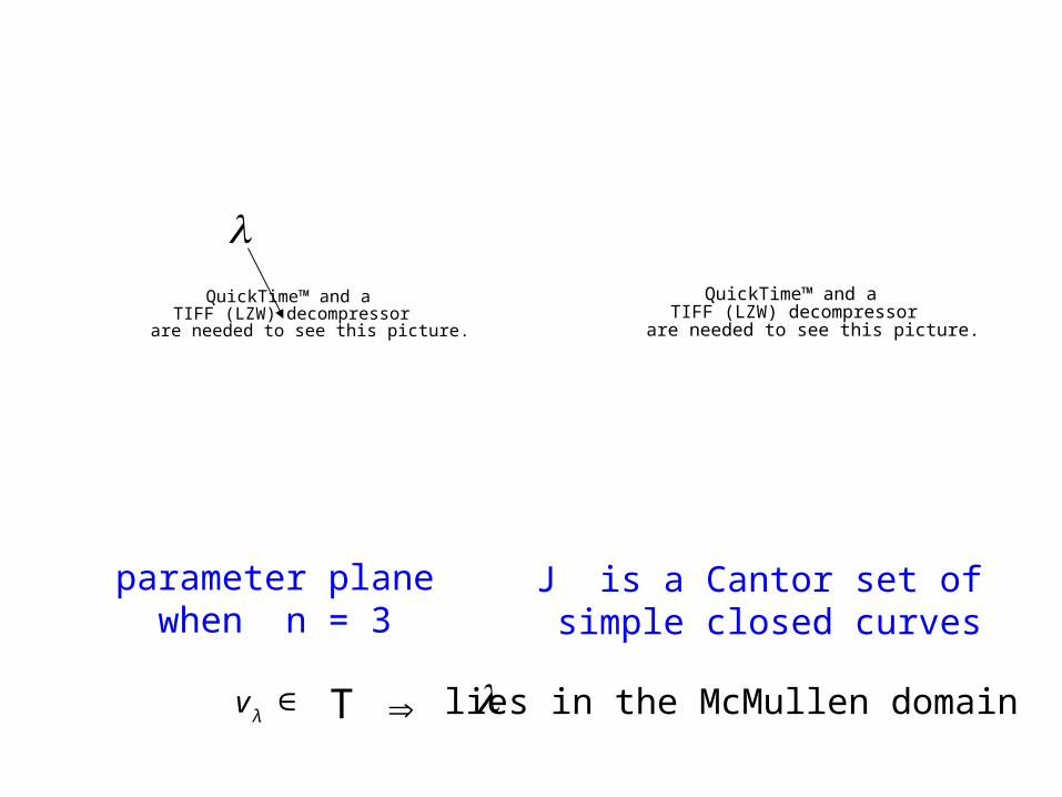
parameter planewhen n = 3
Case 1:

QuickTime™ and aTIFF (LZW) decompressor
are needed to see this picture.
QuickTime™ and aTIFF (LZW) decompressor
are needed to see this picture.
€
vλ∈
€
J ( Fλ
)
€
⇒B is a Cantor set
parameter planewhen n = 3
J is a Cantor set
€
λ

QuickTime™ and aTIFF (LZW) decompressor
are needed to see this picture.
QuickTime™ and aTIFF (LZW) decompressor
are needed to see this picture.
€
vλ∈
€
J ( Fλ
)
€
⇒B is a Cantor set
parameter planewhen n = 3
J is a Cantor set
€
λ

QuickTime™ and aTIFF (LZW) decompressor
are needed to see this picture.
€
vλ∈
€
J ( Fλ
)
€
⇒B is a Cantor set
parameter planewhen n = 3
J is a Cantor set
QuickTime™ and aTIFF (LZW) decompressor
are needed to see this picture.
€
λ

QuickTime™ and aTIFF (LZW) decompressor
are needed to see this picture.
QuickTime™ and aTIFF (LZW) decompressor
are needed to see this picture.
€
vλ∈
€
J ( Fλ
)
€
⇒B is a Cantor set
parameter planewhen n = 3
J is a Cantor set
€
λ

QuickTime™ and aTIFF (LZW) decompressor
are needed to see this picture.
QuickTime™ and aTIFF (LZW) decompressor
are needed to see this picture.
€
vλ∈
€
J ( Fλ
)
€
⇒B is a Cantor set
parameter planewhen n = 3
J is a Cantor set
€
λ

QuickTime™ and aTIFF (LZW) decompressor
are needed to see this picture.
QuickTime™ and aTIFF (LZW) decompressor
are needed to see this picture.
€
vλ∈
€
J ( Fλ
)
€
⇒B is a Cantor set
parameter planewhen n = 3
J is a Cantor set
€
λ

QuickTime™ and aTIFF (LZW) decompressor
are needed to see this picture.
QuickTime™ and aTIFF (LZW) decompressor
are needed to see this picture.
€
vλ∈
€
J ( Fλ
)
€
⇒B is a Cantor set
parameter planewhen n = 3
J is a Cantor set
€
λ

QuickTime™ and aTIFF (LZW) decompressor
are needed to see this picture.
QuickTime™ and aTIFF (LZW) decompressor
are needed to see this picture.
€
vλ∈
€
J ( Fλ
)
€
⇒B is a Cantor set
parameter planewhen n = 3
J is a Cantor set
€
λ
QuickTime™ and aTIFF (LZW) decompressor
are needed to see this picture.
QuickTime™ and aTIFF (LZW) decompressor
are needed to see this picture.
€
vλ∈
€
J ( Fλ
)
€
⇒B is a Cantor set
parameter planewhen n = 3
J is a Cantor set
€
λ

QuickTime™ and aTIFF (LZW) decompressor
are needed to see this picture.
QuickTime™ and aTIFF (LZW) decompressor
are needed to see this picture.
€
vλ∈
€
J ( Fλ
)
€
⇒B is a Cantor set
parameter planewhen n = 3
J is a Cantor set
€
λ

QuickTime™ and aTIFF (LZW) decompressor
are needed to see this picture.
QuickTime™ and aTIFF (LZW) decompressor
are needed to see this picture.
€
vλ∈
€
J ( Fλ
)
€
⇒B is a Cantor set
parameter planewhen n = 3
J is a Cantor set
€
λ
QuickTime™ and aTIFF (LZW) decompressor
are needed to see this picture.
QuickTime™ and aTIFF (LZW) decompressor
are needed to see this picture.
€
vλ∈
€
J ( Fλ
)
€
⇒B is a Cantor set
parameter planewhen n = 3
J is a Cantor set
€
λ

QuickTime™ and aTIFF (LZW) decompressor
are needed to see this picture.
parameter planewhen n = 3
Case 2: the critical values lie in T, not B

QuickTime™ and aTIFF (LZW) decompressor
are needed to see this picture.
€
vλ∈
€
⇒T
parameter planewhen n = 3
€
λ lies in the McMullen domain
€
λ

QuickTime™ and aTIFF (LZW) decompressor
are needed to see this picture.
€
vλ∈
€
⇒T
parameter planewhen n = 3
J is a Cantor set of simple closed curves
€
λ lies in the McMullen domain
€
λQuickTime™ and a
TIFF (LZW) decompressorare needed to see this picture.
Remark: There is no McMullen domain in the case n = 2.

QuickTime™ and aTIFF (LZW) decompressor
are needed to see this picture.
€
vλ∈
€
⇒T
parameter planewhen n = 3
J is a Cantor set of simple closed curves
€
λ lies in the McMullen domain
€
λQuickTime™ and a
TIFF (LZW) decompressorare needed to see this picture.

QuickTime™ and aTIFF (LZW) decompressor
are needed to see this picture.
€
vλ∈
€
⇒T
parameter planewhen n = 3
J is a Cantor set of simple closed curves
€
λ lies in the McMullen domain
€
λQuickTime™ and a
TIFF (LZW) decompressorare needed to see this picture.

QuickTime™ and aTIFF (LZW) decompressor
are needed to see this picture.
€
vλ∈
€
⇒T
parameter planewhen n = 3
J is a Cantor set of simple closed curves
€
λ lies in the McMullen domain
€
λQuickTime™ and a
TIFF (LZW) decompressorare needed to see this picture.

QuickTime™ and aTIFF (LZW) decompressor
are needed to see this picture.
€
vλ∈
€
⇒T
parameter planewhen n = 3
J is a Cantor set of simple closed curves
€
λ lies in the McMullen domain
€
λQuickTime™ and a
TIFF (LZW) decompressorare needed to see this picture.

QuickTime™ and aTIFF (LZW) decompressor
are needed to see this picture.
€
vλ∈
€
⇒T
parameter planewhen n = 3
J is a Cantor set of simple closed curves
€
λ lies in the McMullen domain
€
λQuickTime™ and a
TIFF (LZW) decompressorare needed to see this picture.
QuickTime™ and aTIFF (LZW) decompressor
are needed to see this picture.
€
vλ∈
€
⇒T
parameter planewhen n = 3
J is a Cantor set of simple closed curves
€
λ lies in the McMullen domain
€
λQuickTime™ and a
TIFF (LZW) decompressorare needed to see this picture.

QuickTime™ and aTIFF (LZW) decompressor
are needed to see this picture.
€
⇒T
parameter planewhen n = 3
€
λ lies in a Sierpinski hole
€
Fλ
k(v
λ) ∈
Case 3: the critical orbit eventually lands in the trap door.

QuickTime™ and aTIFF (LZW) decompressor
are needed to see this picture.
€
⇒T
parameter planewhen n = 3
J is an escape time Sierpinski curve
€
λ lies in a Sierpinski hole
€
λ
€
Fλ
k(v
λ) ∈
QuickTime™ and aTIFF (LZW) decompressor
are needed to see this picture.

QuickTime™ and aTIFF (LZW) decompressor
are needed to see this picture.
€
⇒T
parameter planewhen n = 3
€
λ lies in a Sierpinski hole
€
λ
€
Fλ
k(v
λ) ∈
QuickTime™ and aTIFF (LZW) decompressor
are needed to see this picture.
J is an escape time Sierpinski curve

QuickTime™ and aTIFF (LZW) decompressor
are needed to see this picture.
€
⇒T
parameter planewhen n = 3
€
λ lies in a Sierpinski hole
€
λ
€
Fλ
k(v
λ) ∈
QuickTime™ and aTIFF (LZW) decompressor
are needed to see this picture.
J is an escape time Sierpinski curve

QuickTime™ and aTIFF (LZW) decompressor
are needed to see this picture.
€
⇒T
parameter planewhen n = 3
€
λ lies in a Sierpinski hole
€
λ
€
Fλ
k(v
λ) ∈
QuickTime™ and aTIFF (LZW) decompressor
are needed to see this picture.
J is an escape time Sierpinski curve

QuickTime™ and aTIFF (LZW) decompressor
are needed to see this picture.
€
⇒T
parameter planewhen n = 3
€
λ lies in a Sierpinski hole
€
λ
€
Fλ
k(v
λ) ∈
QuickTime™ and aTIFF (LZW) decompressor
are needed to see this picture.
J is an escape time Sierpinski curve

QuickTime™ and aTIFF (LZW) decompressor
are needed to see this picture.
€
⇒T
parameter planewhen n = 3
€
λ lies in a Sierpinski hole
€
λ
€
Fλ
k(v
λ) ∈
QuickTime™ and aTIFF (LZW) decompressor
are needed to see this picture.
J is an escape time Sierpinski curve

QuickTime™ and aTIFF (LZW) decompressor
are needed to see this picture.
€
⇒T
parameter planewhen n = 3
€
λ lies in a Sierpinski hole
€
λ
€
Fλ
k(v
λ) ∈
QuickTime™ and aTIFF (LZW) decompressor
are needed to see this picture.
J is an escape time Sierpinski curve

QuickTime™ and aTIFF (LZW) decompressor
are needed to see this picture.
€
⇒T
parameter planewhen n = 3
€
λ lies in a Sierpinski hole
€
λ
€
Fλ
k(v
λ) ∈
QuickTime™ and aTIFF (LZW) decompressor
are needed to see this picture.
J is an escape time Sierpinski curve

QuickTime™ and aTIFF (LZW) decompressor
are needed to see this picture.
€
⇒T
parameter planewhen n = 3
€
λ lies in a Sierpinski hole
€
λ
€
Fλ
k(v
λ) ∈
QuickTime™ and aTIFF (LZW) decompressor
are needed to see this picture.
J is an escape time Sierpinski curve

QuickTime™ and aTIFF (LZW) decompressor
are needed to see this picture.
€
⇒T
parameter planewhen n = 3
€
λ lies in a Sierpinski hole
€
λ
€
Fλ
k(v
λ) ∈
QuickTime™ and aTIFF (LZW) decompressor
are needed to see this picture.
J is an escape time Sierpinski curve

QuickTime™ and aTIFF (LZW) decompressor
are needed to see this picture.
€
⇒T
parameter planewhen n = 3
€
λ lies in a Sierpinski hole
€
λ
€
Fλ
k(v
λ) ∈
QuickTime™ and aTIFF (LZW) decompressor
are needed to see this picture.
J is an escape time Sierpinski curve

QuickTime™ and aTIFF (LZW) decompressor
are needed to see this picture.
To show that is homeomorphic to
QuickTime™ and aTIFF (LZW) decompressor
are needed to see this picture.

QuickTime™ and aTIFF (LZW) decompressor
are needed to see this picture.
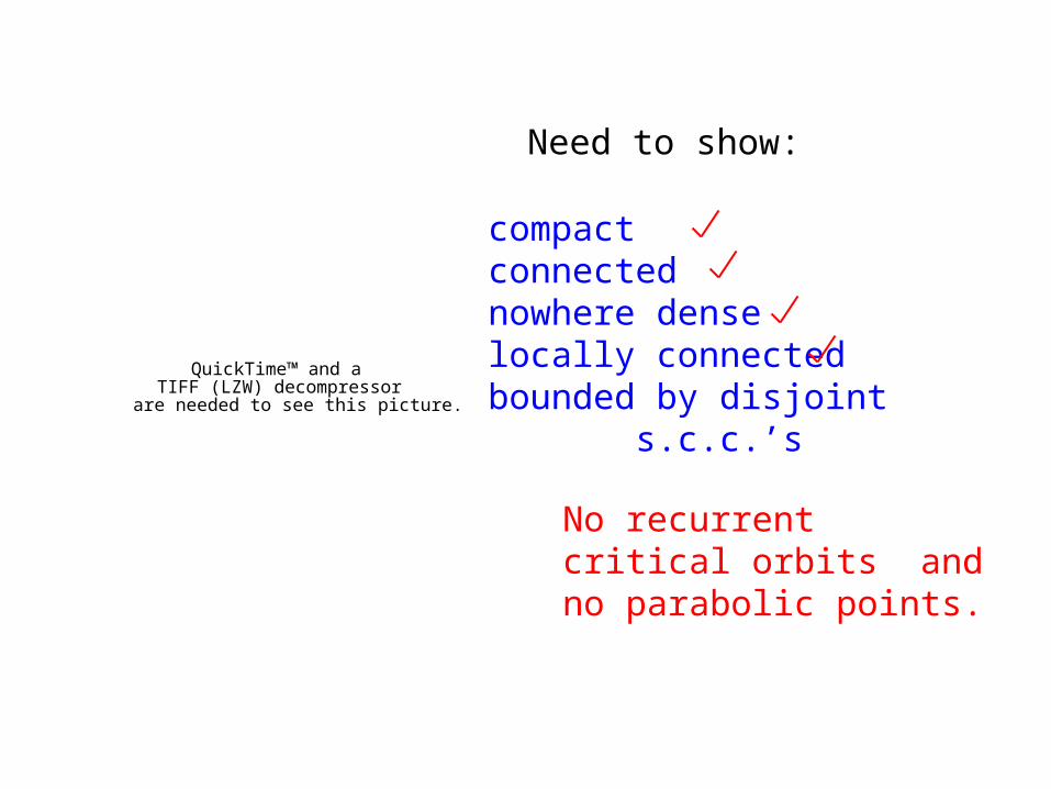
Need to show:
compactconnectednowhere denselocally connectedbounded by disjoint s.c.c.’s

QuickTime™ and aTIFF (LZW) decompressor
are needed to see this picture.
Need to show:
compactconnectednowhere denselocally connectedbounded by disjoint s.c.c.’s
Fatou set is the union of the preimages of B; all disjoint, open disks.

QuickTime™ and aTIFF (LZW) decompressor
are needed to see this picture.
Need to show:
compactconnectednowhere denselocally connectedbounded by disjoint s.c.c.’s
Fatou set is the union of the preimages of B; all disjoint, open disks.

QuickTime™ and aTIFF (LZW) decompressor
are needed to see this picture.
Need to show:
compactconnectednowhere denselocally connectedbounded by disjoint s.c.c.’s
If J contains an open set, then J = C.

QuickTime™ and aTIFF (LZW) decompressor
are needed to see this picture.
Need to show:
compactconnectednowhere denselocally connectedbounded by disjoint s.c.c.’s
If J contains an open set, then J = C.

QuickTime™ and aTIFF (LZW) decompressor
are needed to see this picture.
Need to show:
compactconnectednowhere denselocally connectedbounded by disjoint s.c.c.’s
No recurrent critical orbits and no parabolic points.
QuickTime™ and aTIFF (LZW) decompressor
are needed to see this picture.
Need to show:
compactconnectednowhere denselocally connectedbounded by disjoint s.c.c.’s
No recurrent critical orbits and no parabolic points.

QuickTime™ and aTIFF (LZW) decompressor
are needed to see this picture.
Need to show:
compactconnectednowhere denselocally connectedbounded by disjoint s.c.c.’s
J locally connected, so theboundaries are locally connected. Need to show they are s.c.c.’s. Can only meet at (preimages of) critical points, hence disjoint.

QuickTime™ and aTIFF (LZW) decompressor
are needed to see this picture.
Need to show:
compactconnectednowhere denselocally connectedbounded by disjoint s.c.c.’s
So J is a Sierpinski curve.

Have an exact count of the number of Sierpinski holes:
Theorem (Roesch): Given n, there are exactly (n-1)(2n) Sierpinski holes with escape time k. (k-3)

Have an exact count of the number of Sierpinski holes:
Reason: The equation reduces to a polynomial of degree (n-1)(2n)(k-3) ;we have a Bottcher coordinate on each Sierpinski hole;and so all the roots of this polynomial are distinct. So we have exactly that many “centers” of Sierpinski holes, i.e., parameters for which the critical points all land on 0 and then on .
€
Fλk−1(λ1/2n ) = 0
€
∞
Theorem (Roesch): Given n, there are exactly (n-1)(2n) Sierpinski holes with escape time k. (k-3)

Have an exact count of the number of Sierpinski holes:
QuickTime™ and aTIFF (LZW) decompressor
are needed to see this picture.
n = 3escape time 32 Sierpinski holes
parameter planen = 3
Theorem (Roesch): Given n, there are exactly (n-1)(2n) Sierpinski holes with escape time k. (k-3)

Have an exact count of the number of Sierpinski holes:
QuickTime™ and aTIFF (LZW) decompressor
are needed to see this picture.
n = 3escape time 32 Sierpinski holes
parameter planen = 3
Theorem (Roesch): Given n, there are exactly (n-1)(2n) Sierpinski holes with escape time k. (k-3)

Have an exact count of the number of Sierpinski holes:
QuickTime™ and aTIFF (LZW) decompressor
are needed to see this picture.
n = 3escape time 412 Sierpinski holes
parameter planen = 3
Theorem (Roesch): Given n, there are exactly (n-1)(2n) Sierpinski holes with escape time k. (k-3)

Have an exact count of the number of Sierpinski holes:
QuickTime™ and aTIFF (LZW) decompressor
are needed to see this picture.
n = 3escape time 412 Sierpinski holes
parameter planen = 3
Theorem (Roesch): Given n, there are exactly (n-1)(2n) Sierpinski holes with escape time k. (k-3)

Have an exact count of the number of Sierpinski holes:
n = 4escape time 33 Sierpinski holes
QuickTime™ and aTIFF (LZW) decompressor
are needed to see this picture.
parameter planen = 4
Theorem (Roesch): Given n, there are exactly (n-1)(2n) Sierpinski holes with escape time k. (k-3)

Have an exact count of the number of Sierpinski holes:
n = 4escape time 424 Sierpinski holes
QuickTime™ and aTIFF (LZW) decompressor
are needed to see this picture.
parameter planen = 4
Theorem (Roesch): Given n, there are exactly (n-1)(2n) Sierpinski holes with escape time k. (k-3)

Have an exact count of the number of Sierpinski holes:
n = 4escape time 12 402,653,184 Sierpinski holes
QuickTime™ and aTIFF (LZW) decompressor
are needed to see this picture.
Sorry. I forgot to indicate their locations. parameter plane
n = 4
Theorem (Roesch): Given n, there are exactly (n-1)(2n) Sierpinski holes with escape time k. (k-3)

Given two Sierpinski curve Julia sets, when do we know that the dynamics on them are the same, i.e., the maps are conjugate on the Julia sets?
Main Question:
QuickTime™ and aTIFF (LZW) decompressor
are needed to see this picture.
QuickTime™ and aTIFF (LZW) decompressor
are needed to see this picture.
These sets are homeomorphic, but are the dynamics on them the same?

#1: If and are drawn from the same Sierpinski hole, then the correspondingmaps have the same dynamics, i.e., they are topologically conjugate on their Julia sets.€
λ
€
μ
QuickTime™ and aTIFF (LZW) decompressor
are needed to see this picture.
parameter planen = 4

#1: If and are drawn from the same Sierpinski hole, then the correspondingmaps have the same dynamics, i.e., they are topologically conjugate on their Julia sets.
QuickTime™ and aTIFF (LZW) decompressor
are needed to see this picture.So all these parametershave the same dynamicson their Julia sets.
parameter planen = 4
€
λ
€
μ

#1: If and are drawn from the same Sierpinski hole, then the correspondingmaps have the same dynamics, i.e., they are topologically conjugate on their Julia sets.€
λ
€
μ
QuickTime™ and aTIFF (LZW) decompressor
are needed to see this picture.
parameter planen = 4
This uses quasiconformalsurgery techniques

#1: If and are drawn from the same Sierpinski hole, then the correspondingmaps have the same dynamics, i.e., they are topologically conjugate on their Julia sets.€
λ
€
μ
#2: If these parameters come from Sierpinski holes with different “escape times,” then the maps cannot be conjugate.

QuickTime™ and aTIFF (LZW) decompressor
are needed to see this picture.
QuickTime™ and aTIFF (LZW) decompressor
are needed to see this picture.
€
Fλ (z ) = z 3 +λ
z 3
Two Sierpinski curve Julia sets, so they are homeomorphic.
€
cλ
€
cμ
€
Fμ (z ) = z 3 +μ
z 3

QuickTime™ and aTIFF (LZW) decompressor
are needed to see this picture.
QuickTime™ and aTIFF (LZW) decompressor
are needed to see this picture.
escape time 3 escape time 4
So these maps cannot be topologically conjugate.
€
cλ
€
cμ
€
Fλ (z ) = z 3 +λ
z 3
€
Fμ (z ) = z 3 +μ
z 3
QuickTime™ and aTIFF (LZW) decompressor
are needed to see this picture.
QuickTime™ and aTIFF (LZW) decompressor
are needed to see this picture.
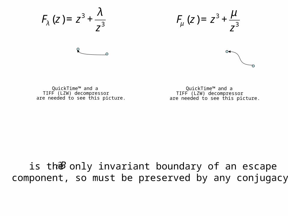
is the only invariant boundary of an escapecomponent, so must be preserved by any conjugacy.
€
∂B
€
Fλ (z ) = z 3 +λ
z 3
€
Fμ (z ) = z 3 +μ
z 3
QuickTime™ and aTIFF (LZW) decompressor
are needed to see this picture.
QuickTime™ and aTIFF (LZW) decompressor
are needed to see this picture.
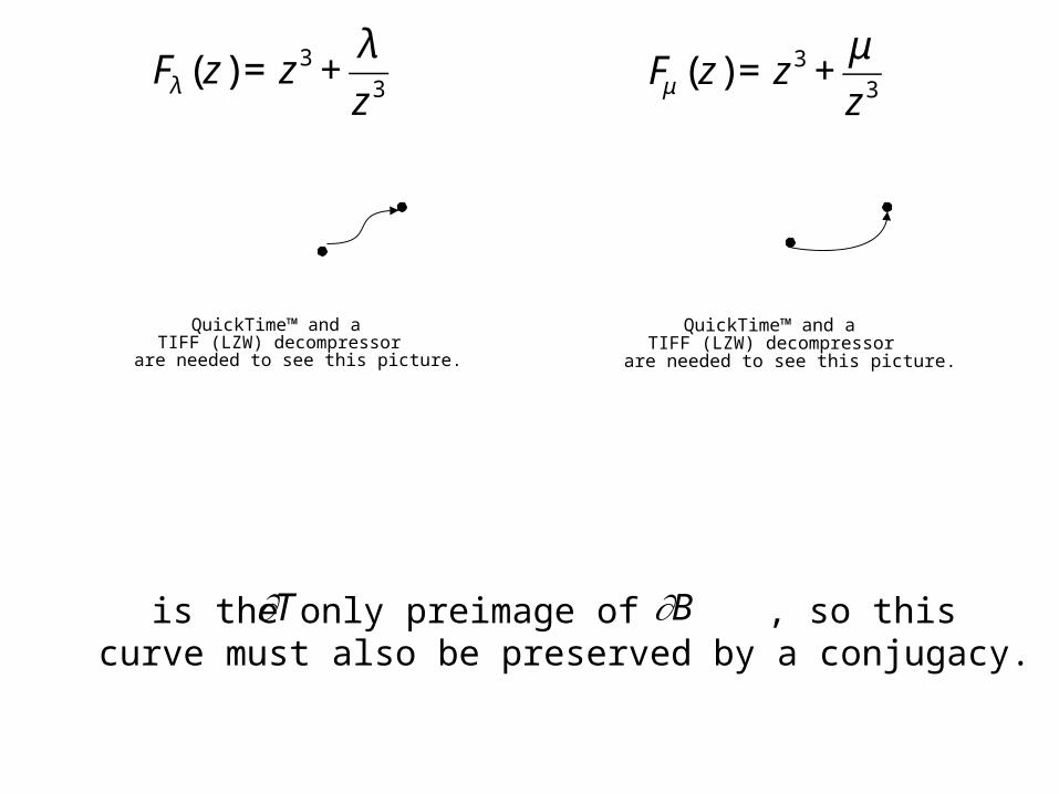
is the only preimage of , so this curve must also be preserved by a conjugacy.
€
∂B
€
∂T
€
Fλ (z ) = z 3 +λ
z 3
€
Fμ (z ) = z 3 +μ
z 3

QuickTime™ and aTIFF (LZW) decompressor
are needed to see this picture.
QuickTime™ and aTIFF (LZW) decompressor
are needed to see this picture.
If a boundary component is mapped toafter k iterations, its image under the conjugacy must also have this property,and so forth.....
€
∂T
€
Fλ (z ) = z 3 +λ
z 3
€
Fμ (z ) = z 3 +μ
z 3
QuickTime™ and aTIFF (LZW) decompressor
are needed to see this picture.
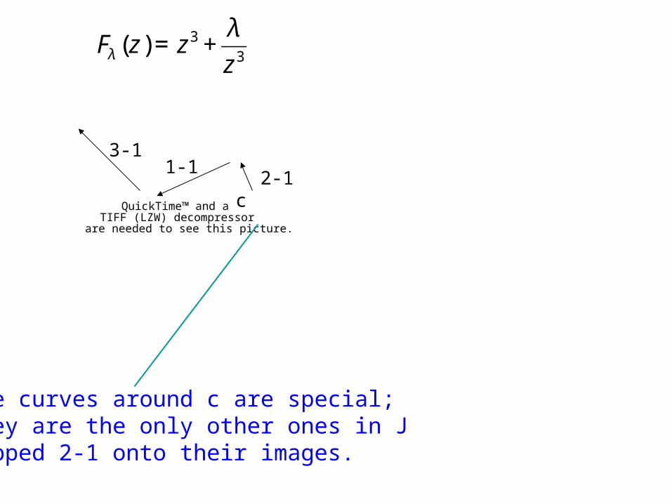
2-11-1
3-1
The curves around c are special; they are the only other ones in Jmapped 2-1 onto their images.
c
€
Fλ (z ) = z 3 +λ
z 3

QuickTime™ and aTIFF (LZW) decompressor
are needed to see this picture.
QuickTime™ and aTIFF (LZW) decompressor
are needed to see this picture.
2-11-1
3-1
2-1
3-11-11-1
This bounding region takes 3 iterates to land on the
boundary of B.
But this bounding region takes 4 iterates to land, so
these maps are not conjugate.
€
Fλ (z ) = z 3 +λ
z 3
€
Fμ (z ) = z 3 +μ
z 3

For this it suffices to consider the centers of the Sierpinski holes; i.e., parameter values
for which for some k 3.
€
Fλk(cλ ) = ∞
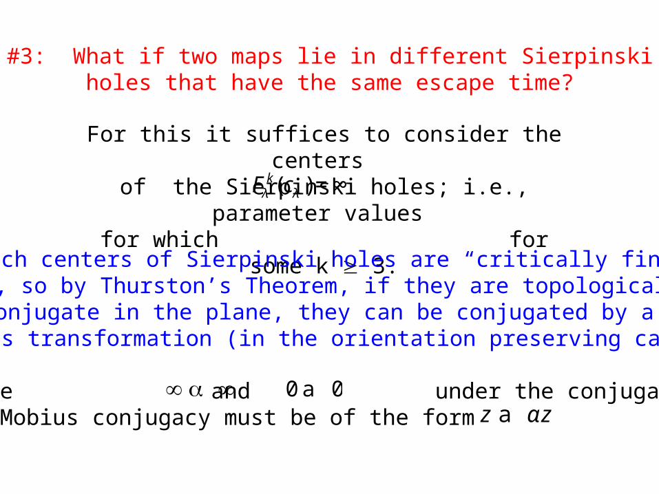
#3: What if two maps lie in different Sierpinski holes that have the same escape time?

#3: What if two maps lie in different Sierpinski holes that have the same escape time?
For this it suffices to consider the centers of the Sierpinski holes; i.e., parameter values
for which for some k 3.
Two such centers of Sierpinski holes are “critically finite” maps, so by Thurston’s Theorem, if they are topologically
conjugate in the plane, they can be conjugated by a Mobius transformation (in the orientation preserving case).
€
Fλk(cλ ) = ∞
#3: What if two maps lie in different Sierpinski holes that have the same escape time?
For this it suffices to consider the centers of the Sierpinski holes; i.e., parameter values
for which for some k 3.
Two such centers of Sierpinski holes are “critically finite” maps, so by Thurston’s Theorem, if they are topologically
conjugate in the plane, they can be conjugated by a Mobius transformation (in the orientation preserving case).
Since and under the conjugacy,the Mobius conjugacy must be of the form .
€
∞ a ∞
€
0 a 0
€
z a αz
€
Fλk(cλ ) = ∞

€
h(Fλ (z)) = Fμ (h(z))then:
€
α zn +λ
zn
⎛
⎝ ⎜
⎞
⎠ ⎟=αzn +
αλ
zn=α nzn +
μ
α nzn
If we have a conjugacy
€
h(z) =αz

If we have a conjugacy
€
h(Fλ (z)) = Fμ (h(z))
€
h(z) =αz
then:
€
α zn +λ
zn
⎛
⎝ ⎜
⎞
⎠ ⎟=αzn +
αλ
zn=α nzn +
μ
α nzn
Comparing coefficients:
€
αn−1 =1

€
h(Fλ (z)) = Fμ (h(z))then:
€
α zn +λ
zn
⎛
⎝ ⎜
⎞
⎠ ⎟=αzn +
αλ
zn=α nzn +
μ
α nzn
Comparing coefficients:
€
αn−1 =1
€
μ =α2λ
If we have a conjugacy
€
h(z) =αz

€
h(Fλ (z)) = Fμ (h(z))then:
€
α zn +λ
zn
⎛
⎝ ⎜
⎞
⎠ ⎟=αzn +
αλ
zn=α nzn +
μ
α nzn
Comparing coefficients:
€
αn−1 =1
€
μ =α2λ
Easy check --- for the orientation reversing case:
is conjugate to via
€
Fλ
€
Fλ
€
h(z) = z
If we have a conjugacy
€
h(z) =αz

Theorem. If and are centers of Sierpinski holes, then iff or whereis a primitive root of unity; then any twoparameters drawn from these holes have the samedynamics.
€
Fλ ≈ Fμ
€
α
€
(n −1)st
€
μ
€
λ
n = 3: Only and are conjugatecenters since
€
λ
€
λ
€
αλ
€
α2λ
€
λ
€
λ
€
αλ
€
α2λ, , , , ,n = 4: Only
are conjugate centers where .
€
α 3 =1
€
μ =α2 jλ
€
μ =α2 jλ
€
α =−1

QuickTime™ and aTIFF (LZW) decompressor
are needed to see this picture.
n = 3, escape time 4, 12 Sierpinski holes,but only six conjugacy classes
€
λ
€
λconjugate centers: ,

QuickTime™ and aTIFF (LZW) decompressor
are needed to see this picture.
n = 3, escape time 4, 12 Sierpinski holes,but only six conjugacy classes
€
λ
€
λconjugate centers: ,

QuickTime™ and aTIFF (LZW) decompressor
are needed to see this picture.
n = 3, escape time 4, 12 Sierpinski holes,but only six conjugacy classes
€
λ
€
λconjugate centers: ,

QuickTime™ and aTIFF (LZW) decompressor
are needed to see this picture.
n = 3, escape time 4, 12 Sierpinski holes,but only six conjugacy classes
€
λ
€
λconjugate centers: ,

QuickTime™ and aTIFF (LZW) decompressor
are needed to see this picture.
€
αλ
€
α2λ
€
λ
€
λ
€
αλ
€
α2λ, , , , , where
€
α 3 =1
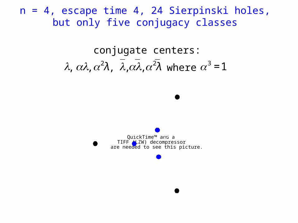
n = 4, escape time 4, 24 Sierpinski holes,but only five conjugacy classes
conjugate centers:

QuickTime™ and aTIFF (LZW) decompressor
are needed to see this picture.
€
αλ
€
α2λ
€
λ
€
λ
€
αλ
€
α2λ, , , , , where
€
α 3 =1
n = 4, escape time 4, 24 Sierpinski holes,but only five conjugacy classes
conjugate centers:

QuickTime™ and aTIFF (LZW) decompressor
are needed to see this picture.
€
αλ
€
α2λ
€
λ
€
λ
€
αλ
€
α2λ, , , , , where
€
α 3 =1
n = 4, escape time 4, 24 Sierpinski holes,but only five conjugacy classes
conjugate centers:
QuickTime™ and aTIFF (LZW) decompressor
are needed to see this picture.
€
αλ
€
α2λ
€
λ
€
λ
€
αλ
€
α2λ, , , , , where
€
α 3 =1
n = 4, escape time 4, 24 Sierpinski holes,but only five conjugacy classes
conjugate centers:

QuickTime™ and aTIFF (LZW) decompressor
are needed to see this picture.
€
αλ
€
α2λ
€
λ
€
λ
€
αλ
€
α2λ, , , , , where
€
α 3 =1
n = 4, escape time 4, 24 Sierpinski holes,but only five conjugacy classes
conjugate centers:

Theorem: For any n there are exactly (n-1) (2n) Sierpinski holes with escape time k. The number ofdistinct conjugacy classes is given by:
k-3
a. (2n) when n is odd;k-3
b. (2n) /2 + 2 when n is even.k-3 k-4

QuickTime™ and aTIFF (LZW) decompressor
are needed to see this picture.
QuickTime™ and aTIFF (LZW) decompressor
are needed to see this picture.
For n odd, there are no Sierpinski holes along the real axis,so there are exactly n - 1 conjugate Sierpinski holes.
n = 3 n = 5

For n even, there is a “Cantor necklace” along the negativeaxis, so there are some “real” Sierpinski holes,
n = 4
QuickTime™ and aTIFF (LZW) decompressor
are needed to see this picture.

For n even, there is a “Cantor necklace” along the negativeaxis, so there are some “real” Sierpinski holes,
n = 4
QuickTime™ and aTIFF (LZW) decompressor
are needed to see this picture.

For n even, there is a “Cantor necklace” along the negativeaxis, so there are some “real” Sierpinski holes,
n = 4 magnification
QuickTime™ and aTIFF (LZW) decompressor
are needed to see this picture.
QuickTime™ and aTIFF (LZW) decompressor
are needed to see this picture. M

For n even, there is a “Cantor necklace” along the negativeaxis, so there are some “real” Sierpinski holes,
n = 4 magnification
QuickTime™ and aTIFF (LZW) decompressor
are needed to see this picture.
QuickTime™ and aTIFF (LZW) decompressor
are needed to see this picture. M34 4
5 5

For n even, there is a “Cantor necklace” along the negativeaxis, so we can count the number of “real” Sierpinski holes,
and there are exactly n - 1 conjugate holes in this case:
n = 4 magnification
QuickTime™ and aTIFF (LZW) decompressor
are needed to see this picture.
QuickTime™ and aTIFF (LZW) decompressor
are needed to see this picture. M34 4
5 5

For n even, there are also 2(n - 1) “complex” Sierpinski holes that have conjugate dynamics:
n = 4 magnification
QuickTime™ and aTIFF (LZW) decompressor
are needed to see this picture.
QuickTime™ and aTIFF (LZW) decompressor
are needed to see this picture. M

QuickTime™ and aTIFF (LZW) decompressor
are needed to see this picture.
n = 4: 402,653,184 Sierpinski holes with escape time 12; 67,108,832 distinct conjugacy classes.
Sorry. I again forgot to indicate their locations.

QuickTime™ and aTIFF (LZW) decompressor
are needed to see this picture.
n = 4: 402,653,184 Sierpinski holes with escape time 12; 67,108,832 distinct conjugacy classes.
Problem: Describe the dynamics on these different conjugacy classes.

Other ways that Sierpinski curve Julia sets arise:
1. Buried points in Cantor necklaces;
2. Main cardioids in buried Mandelbrot sets;
3. Structure around the McMullen domain;
4. Other families of rational maps;
5. The difference between n = 2 and n >2 ;
6. Major applications

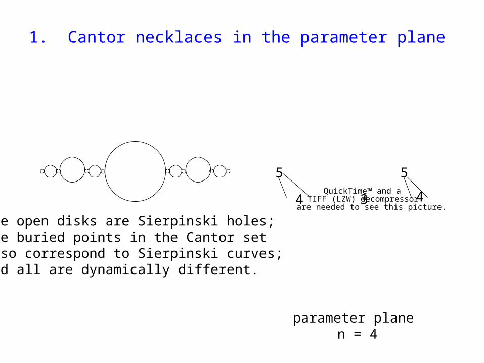
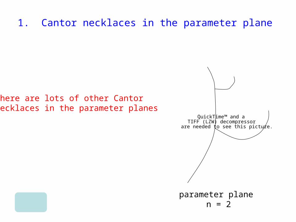
1. Cantor necklaces in the parameter plane
parameter plane n = 4
QuickTime™ and aTIFF (LZW) decompressor
are needed to see this picture.MThe necklace is the Cantor middle thirds set with disks replacing removed intervals.

1. Cantor necklaces in the parameter plane
parameter plane n = 4
QuickTime™ and aTIFF (LZW) decompressor
are needed to see this picture.MThere is a Cantor necklace along the negative real axis

parameter plane n = 4
QuickTime™ and aTIFF (LZW) decompressor
are needed to see this picture.
The open disks are Sierpinski holes
34 4
5 5
1. Cantor necklaces in the parameter plane

parameter plane n = 4
QuickTime™ and aTIFF (LZW) decompressor
are needed to see this picture.
The open disks are Sierpinski holes;the buried points in the Cantor setalso correspond to Sierpinski curves;
34 4
5 5
1. Cantor necklaces in the parameter plane
parameter plane n = 4
QuickTime™ and aTIFF (LZW) decompressor
are needed to see this picture.
The open disks are Sierpinski holes;the buried points in the Cantor setalso correspond to Sierpinski curves;and all are dynamically different.
34 4
5 5
1. Cantor necklaces in the parameter plane

The “endpoints” in the Cantor set (parameters on the boundaries ofthe Sierpinski holes) do not correspond to Sierpinski curves.
1. Cantor necklaces in the parameter plane
A “hybrid” Sierpinski curve;some boundary curves meet.
QuickTime™ and aTIFF (LZW) decompressor
are needed to see this picture.

parameter plane n = 2
There are lots of other Cantornecklaces in the parameter planes.
QuickTime™ and aTIFF (LZW) decompressor
are needed to see this picture.
1. Cantor necklaces in the parameter plane
parameter plane n = 2
There are lots of other Cantornecklaces in the parameter planes.
QuickTime™ and aTIFF (LZW) decompressor
are needed to see this picture.
1. Cantor necklaces in the parameter plane

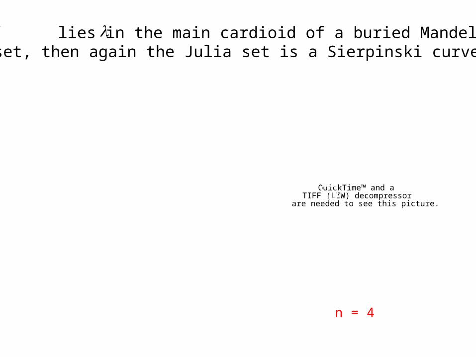
2. If lies in the main cardioid of a buried Mandelbrot set, then again the Julia set is a Sierpinski curve.
QuickTime™ and aTIFF (LZW) decompressor
are needed to see this picture.
n = 4
€
λ
QuickTime™ and aTIFF (LZW) decompressor
are needed to see this picture.
n = 4
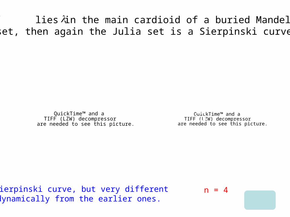
2. If lies in the main cardioid of a buried Mandelbrot set, then again the Julia set is a Sierpinski curve.
€
λ

QuickTime™ and aTIFF (LZW) decompressor
are needed to see this picture.
n = 4
QuickTime™ and aTIFF (LZW) decompressor
are needed to see this picture.
2. If lies in the main cardioid of a buried Mandelbrot set, then again the Julia set is a Sierpinski curve.
€
λ

QuickTime™ and aTIFF (LZW) decompressor
are needed to see this picture.
n = 4
QuickTime™ and aTIFF (LZW) decompressor
are needed to see this picture.
A Sierpinski curve, but very different dynamically from the earlier ones.
2. If lies in the main cardioid of a buried Mandelbrot set, then again the Julia set is a Sierpinski curve.
€
λ
QuickTime™ and aTIFF (LZW) decompressor
are needed to see this picture.
n = 4
QuickTime™ and aTIFF (LZW) decompressor
are needed to see this picture.
A Sierpinski curve, but very different dynamically from the earlier ones.
2. If lies in the main cardioid of a buried Mandelbrot set, then again the Julia set is a Sierpinski curve.
€
λ

QuickTime™ and aTIFF (LZW) decompressor
are needed to see this picture.
n = 4
QuickTime™ and aTIFF (LZW) decompressor
are needed to see this picture.
A Sierpinski curve, but very different dynamically from the earlier ones.
2. If lies in the main cardioid of a buried Mandelbrot set, then again the Julia set is a Sierpinski curve.
€
λ

n = 3
3. If n > 2, there are uncountably many simpleclosed curves surrounding the McMullen domain;
all these parameters are (non-escape) Sierpinski curves.
QuickTime™ and aTIFF (LZW) decompressor
are needed to see this picture.

n = 3
QuickTime™ and aTIFF (LZW) decompressor
are needed to see this picture.
QuickTime™ and aTIFF (LZW) decompressor
are needed to see this picture.
3. If n > 2, there are uncountably many simpleclosed curves surrounding the McMullen domain;
all these parameters are (non-escape) Sierpinski curves.

n = 3
QuickTime™ and aTIFF (LZW) decompressor
are needed to see this picture.
QuickTime™ and aTIFF (LZW) decompressor
are needed to see this picture.
All non-symmetric parameters on these curves have non-conjugate dynamics.
3. If n > 2, there are uncountably many simpleclosed curves surrounding the McMullen domain;
all these parameters are (non-escape) Sierpinski curves.

QuickTime™ and aTIFF (LZW) decompressor
are needed to see this picture.€
γ2
10 centers
n = 3
If n > 2, there are also countably many different simple closed curves accumulating on the McMullen domain. Each alternately passes through centers of Sierpinski holes and centers of baby Mandelbrot sets (j > 1).
€
γj
€
(n − 2)n j +1
€
γj

QuickTime™ and aTIFF (LZW) decompressor
are needed to see this picture.
€
γ3
28 centers
n = 3
If n > 2, there are also countably many different simple closed curves accumulating on the McMullen domain. Each alternately passes through centers of Sierpinski holes and centers of baby Mandelbrot sets (j > 1).
€
γj
€
(n − 2)n j +1
€
γj

QuickTime™ and aTIFF (LZW) decompressor
are needed to see this picture.
€
γ4
82 centers
n = 3
If n > 2, there are also countably many different simple closed curves accumulating on the McMullen domain. Each alternately passes through centers of Sierpinski holes and centers of baby Mandelbrot sets (j > 1).
€
γj
€
(n − 2)n j +1
€
γj

QuickTime™ and aTIFF (LZW) decompressor
are needed to see this picture.
n = 3
€
γ13 passes through1,594,324 centers.
€
γ13
If n > 2, there are also countably many different simple closed curves accumulating on the McMullen domain. Each alternately passes through centers of Sierpinski holes and centers of baby Mandelbrot sets (j > 1).
€
γj
€
(n − 2)n j +1
€
γj

QuickTime™ and aTIFF (LZW) decompressor
are needed to see this picture.
As before, all non-symmetrically locatedcenters havedifferent dynamics.
n = 3
If n > 2, there are also countably many different simple closed curves accumulating on the McMullen domain. Each alternately passes through centers of Sierpinski holes and centers of baby Mandelbrot sets (j > 1).
€
γj
€
(n − 2)n j +1
€
γj
€
γ13
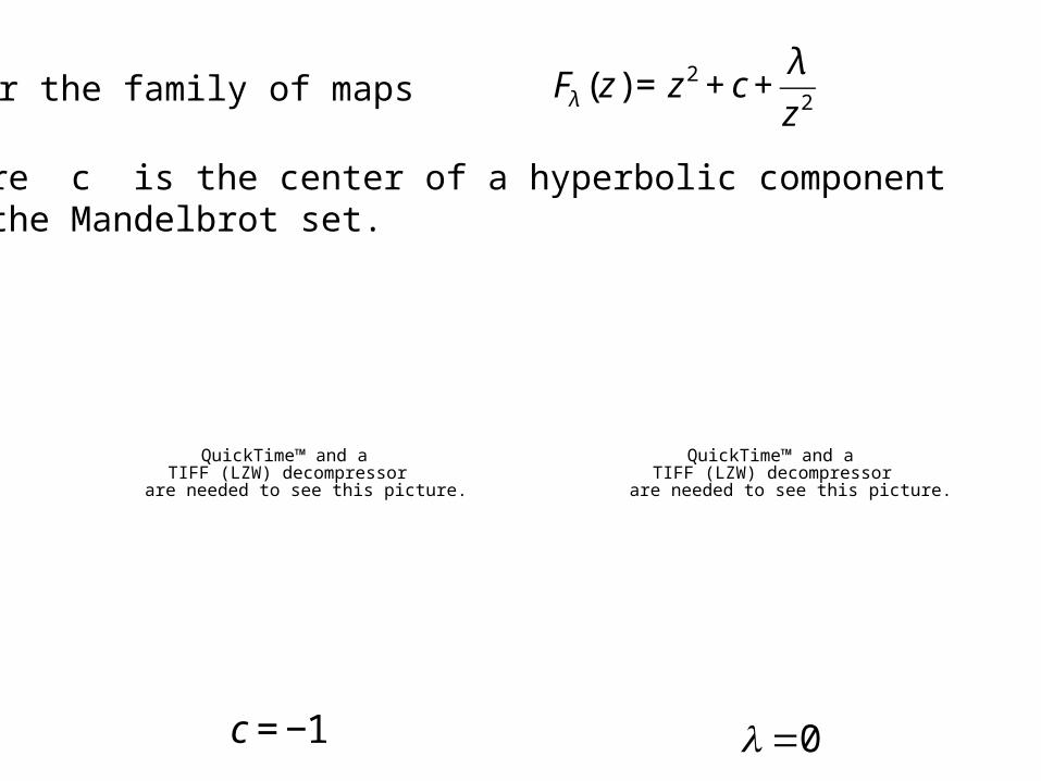
4. Consider the family of maps
where c is the center of a hyperbolic component of the Mandelbrot set.
€
Fλ (z ) = z 2 + c +λ
z 2
QuickTime™ and aTIFF (LZW) decompressor
are needed to see this picture.
€
λ =0
€
c = −1
QuickTime™ and aTIFF (LZW) decompressor
are needed to see this picture.

€
Fλ (z ) = z 2 + c +λ
z 2
€
c = −.12 +.75i
QuickTime™ and aTIFF (LZW) decompressor
are needed to see this picture.
4. Consider the family of maps
where c is the center of a hyperbolic component of the Mandelbrot set.
QuickTime™ and aTIFF (LZW) decompressor
are needed to see this picture.
€
λ =0

QuickTime™ and aTIFF (LZW) decompressor
are needed to see this picture.
QuickTime™ and aTIFF (LZW) decompressor
are needed to see this picture.
€
λ ≠0, the Julia set again expodes.When

QuickTime™ and aTIFF (LZW) decompressor
are needed to see this picture.
QuickTime™ and aTIFF (LZW) decompressor
are needed to see this picture.
€
λ ≠0, the Julia set again expodes.When

QuickTime™ and aTIFF (LZW) decompressor
are needed to see this picture.
€
λ ≠0, the Julia set again expodes.When
QuickTime™ and aTIFF (LZW) decompressor
are needed to see this picture.

QuickTime™ and aTIFF (LZW) decompressor
are needed to see this picture.
€
λ ≠0, the Julia set again expodes.When
QuickTime™ and aTIFF (LZW) decompressor
are needed to see this picture.

€
λ ≠0, the Julia set again expodes.When
QuickTime™ and aTIFF (LZW) decompressor
are needed to see this picture.
QuickTime™ and aTIFF (LZW) decompressor
are needed to see this picture.
A doubly-invertedDouady rabbit.

QuickTime™ and aTIFF (LZW) decompressor
are needed to see this picture.
QuickTime™ and aTIFF (LZW) decompressor
are needed to see this picture.
If you chop off the “ears” of each internal rabbit in each component of the original Fatou set, then what’s left is another Sierpinski curve (provided that both of the critical orbits eventually escape).


The case n = 2 is very different from (and much more difficult than) the case n > 2.
n = 3 n = 2
QuickTime™ and aTIFF (LZW) decompressor
are needed to see this picture.
QuickTime™ and aTIFF (LZW) decompressor
are needed to see this picture.

One difference: there is a McMullen domain whenn > 2, but no McMullen domain when n = 2
QuickTime™ and aTIFF (LZW) decompressor
are needed to see this picture.
QuickTime™ and aTIFF (LZW) decompressor
are needed to see this picture.
n = 3 n = 2

One difference: there is a McMullen domain whenn > 2, but no McMullen domain when n = 2
QuickTime™ and aTIFF (LZW) decompressor
are needed to see this picture.
QuickTime™ and aTIFF (LZW) decompressor
are needed to see this picture.
n = 3 n = 2

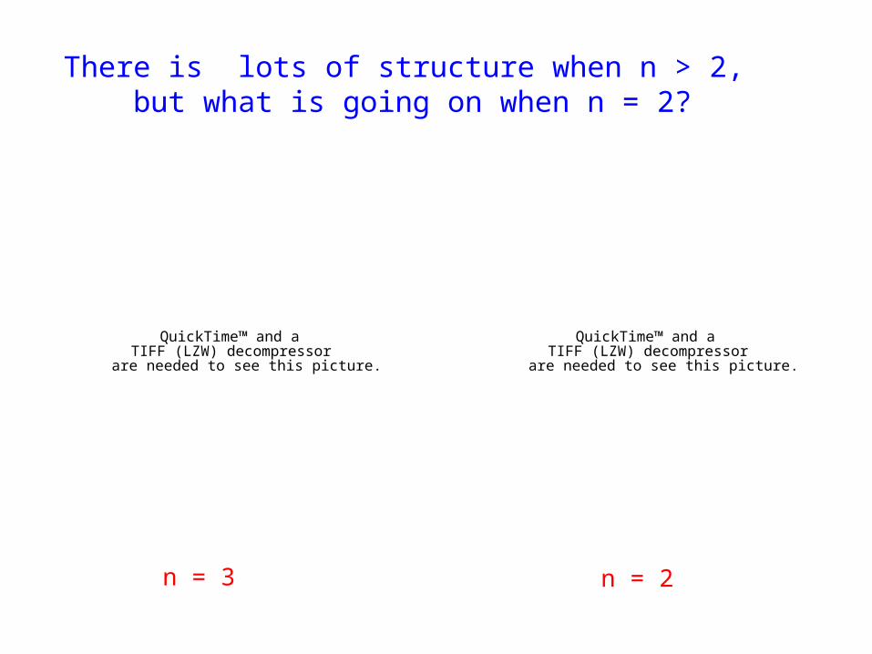
There is lots of structure when n > 2, but what is going on when n = 2?
n = 3 n = 2
QuickTime™ and aTIFF (LZW) decompressor
are needed to see this picture.
QuickTime™ and aTIFF (LZW) decompressor
are needed to see this picture.

There is lots of structure when n > 2, but what is going on when n = 2?
n = 3 n = 2
QuickTime™ and aTIFF (LZW) decompressor
are needed to see this picture.
QuickTime™ and aTIFF (LZW) decompressor
are needed to see this picture.
There is lots of structure when n > 2, but what is going on when n = 2?
n = 3 n = 2
QuickTime™ and aTIFF (LZW) decompressor
are needed to see this picture.
QuickTime™ and aTIFF (LZW) decompressor
are needed to see this picture.

Another difference: as
n = 3 n = 2
QuickTime™ and aTIFF (LZW) decompressor
are needed to see this picture.
QuickTime™ and aTIFF (LZW) decompressor
are needed to see this picture.
€
λ → 0,
€
Fλ2(cλ ) →∞
€
Fλ2(cλ ) →1/ 4
when n > 2when n = 2

Also, not much is happening for the Julia sets near when n > 2
n = 3
QuickTime™ and aTIFF (LZW) decompressor
are needed to see this picture.
€
λ =.01
QuickTime™ and aTIFF (LZW) decompressor
are needed to see this picture.
€
λ =0
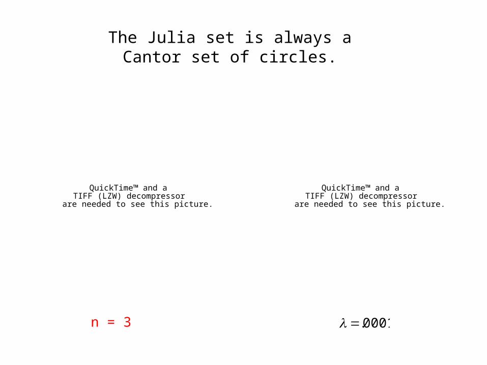
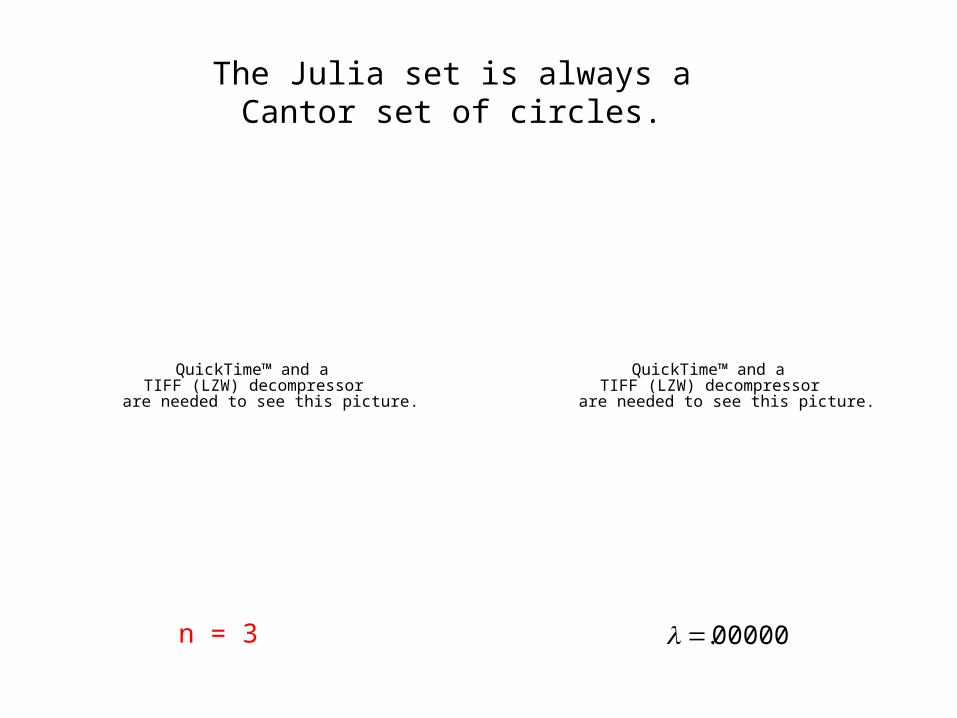
The Julia set is always aCantor set of circles.
n = 3
QuickTime™ and aTIFF (LZW) decompressor
are needed to see this picture.
QuickTime™ and aTIFF (LZW) decompressor
are needed to see this picture.
€
λ =.0001
n = 3
QuickTime™ and aTIFF (LZW) decompressor
are needed to see this picture.
The Julia set is always aCantor set of circles.
QuickTime™ and aTIFF (LZW) decompressor
are needed to see this picture.
€
λ =.000001

The Julia set is always aCantor set of circles.
QuickTime™ and aTIFF (LZW) decompressor
are needed to see this picture.
€
λ =.000001
There is always a round annulus of some fixed width in the Fatou set,
so the Fatou set is “large.”

n = 2
But when n = 2, lots of things happen near the origin;in fact, the Julia sets converge to the unit disk as
QuickTime™ and aTIFF (LZW) decompressor
are needed to see this picture.
€
λ → 0
disk-converge

Here’s the parameter plane when n = 2:
QuickTime™ and aTIFF (LZW) decompressor
are needed to see this picture.

Qu
ickTim
e™
an
d a
TIF
F (
LZ
W)
decom
pre
sso
rare
nee
de
d t
o s
ee t
his
pic
ture
.
Rotate it by 90 degrees:
and this object appears everywhere.....

QuickTime™ and aTIFF (LZW) decompressor
are needed to see this picture.