dynamic demand and mean-ﬁeld games

Dynamic demand and mean-field gamesDario Bauso

Abstract—Within the realm of smart buildings and smart cities,dynamic response management is playing an ever-increasingrole thus attracting the attention of scientists from differentdisciplines. Dynamic demand response management involves aset of operations aiming at decentralizing the control of loadsin large and complex power networks. Each single applianceis fully responsive and readjusts its energy demand to theoverall network load. A main issue is related to mains frequencyoscillations resulting from an unbalance between supply anddemand. In a nutshell, this paper contributes to the topic byequipping each signal consumer with strategic insight. In partic-ular, we highlight three main contributions and a few other minorcontributions. First, we design a mean-field game for a populationof thermostatically controlled loads (TCLs), study the mean-fieldequilibrium for the deterministic mean-field game and investigateon asymptotic stability for the microscopic dynamics. Second, weextend the analysis and design to uncertain models which involveboth stochastic or deterministic disturbances. This leads to robustmean-field equilibrium strategies guaranteeing stochastic andworst-case stability, respectively. Minor contributions involve theuse of stochastic control strategies rather than deterministic, andsome numerical studies illustrating the efficacy of the proposedstrategies.

Index Terms—mean-field games, stochastic stability, powernetworks

I. INTRODUCTION

Demand response involves a set of operations aiming atdecentralizing load control in power networks [1], [12], [13],[28]. In particular, it calls for the alteration of the timing orof the total electricity by end-use customers from their normalconsumption patterns in response to changes in the price ofelectricity. This is possible also through the design of incentivepayments to induce lower electricity use at off-peak times.

A communication protocol aggregates information on past,current and forecasted demand and transmits it to each loadcontroller, which will increase or decrease the proper load. Thenovelty of this paper is that fully responsive load control isobtained by enhancing the intelligence on the demand side ofthe grid. This leads to a less-prescriptive environment in whichthe loads, rather than being pre-programmed to adopt specificswitching behaviors, are designed as intelligent appliancesselecting their switching behaviors as best-responses to thepopulation behavior. The population behavior is sensed by theindividual appliances through the mains frequency state. In this

Research supported by the PRIN 20103S5RN3 “Robust decision making inmarkets and organization”. A short version of this paper including only thedeterministic case has appeared in a chapter of the book [7]. The Stochasticcase in Section 4.2 and the model mis-specification in Section 4.3 areadditional contributions.

Dario Bauso is with the Department of Automatic Control and SystemsEngineering, The University of Sheffield, Mappin Street Sheffield, S1 3JD,United Kingdom, and with the Dipartimento di Ingegneria Chimica, Ges-tionale, Informatica, Meccanica, Universita di Palermo, V.le delle Scienze,90128 Palermo, Italy. {[email protected]}

paper, fully responsive load control is reviewed in the contextof thermostatically controlled loads (TCLs), in smart buildingsor plug-in electric vehicles [2], [21], [22], [26].

A first idea is to use stochastic strategies rather thandeterministic as in [2], [4]. Each TCL selects a probabilitywith which to switch on and off. Thus a probability value of12 means that the TCL is 50% on and 50% off. It has beenshown in [2], [4] that stochastic response strategies outperformdeterministic ones, especially in terms of attenuating the mainsfrequency oscillations. These are due to the unbalance betweenenergy demand and supply (see e.g. [23]). The mains fre-quency usually needs to be stabilized around a nominal value(50 Hz in Europe). If electricity demand exceeds generationthen frequency will decline, and vice versa.

The model used in this paper is as follows. Each singleTCL is a player and is characterized by two state variables,the temperature and the functioning mode. The state dynamicsof a TCL — henceforth referred to as microscopic dynamics— describes the time evolution of its temperature and modein the form of a linear ordinary differential equation in thedeterministic case, and of a stochastic differential equationin the stochastic case. Such dynamics is different from thedynamics of the aggregate temperature and functioning modeof the whole population, which is henceforth referred to asmacroscopic dynamics. In addition to the state dynamics, eachTCL is programmed with a given finite-horizon cost functionalthat accounts for i) energy consumption, ii) deviation ofmains frequency from the nominal one, and iii) deviationof the TCL’s temperature from a reference value. Bringingtogether in the objective functional both individual costs (inthe form of energy consumption and deviation from a referencetemperature) and common costs (in the form of the individualcontribution to the deviation of the mains frequency from thenominal one) is original to the best of the author’s knowledge.More formally, the mains frequency involved in specifics ii)mentioned above is used in a cross-coupling mean-field termthat incentivizes the TCL to switch to off if the mainsfrequency is below the nominal value and to switch to onif the mains frequency is above the nominal value. In otherwords, the cross-coupling mean-field term models all kinds ofincentive payments, benefits, or smart pricing policies aimingat shifting demand from high-peak to off-peak periods.

A. Highlights of contributions

This paper provides three main results. First, in the spirit ofprescriptive game theory and mechanism design [3] we designa mean-field game for the TCLs application, study the mean-field equilibrium for the deterministic mean-field game and in-vestigate on asymptotic stability for the microscopic dynamics.Asymptotic stability means that both the temperature and the

mode functioning of each TCL converge to the reference value.A second result relates to the stochastic case, characterized bya stochastic disturbance in the form of a Brownian motionin the microscopic dynamics. After establishing a mean-fieldequilibrium, we provide some results on stochastic stability.In particular, we focus on two distinct scenarios. In onecase, we assume that the stochastic disturbance expires ina neighborhood of the origin. This reflects in having theBrownian motion coefficients linear in the state. The resultingdynamics is well-known in the literature as geometric Brow-nian motion. As for any geometric Brownian motion, we canstudy conditions for it to be stochastically stable. This meansthat the state trajectories are moment bounded. In a secondcase, the stochastic disturbance is independent on the state andthe Brownian motion coefficients are constant. This leads to adynamics which resembles the Langevin equation. Followingwell-known results on the Langevin equation, the dynamics isproven to be stochastically stable in the second-moment. Anexpository work on stochastic analysis and stability is [20].A third result deals with robustness for the microscopicdynamics. The dynamics is now influenced by an additionaladversarial disturbance, with bounded resource or energy.Even for this case, we study the mean-field equilibrium andinvestigate on conditions that guarantee worst-case stability.The stochastic stability analysis and the worst-case analysisunder adversarial disturbances add originality to the mean-field game approach.

B. Literature overview

We introduce next two streams of literature. One is relatedto dynamic response management, while the second one isabout the theory of differential games with a large number ofindistinguishable players, also known as mean-field games.

1) Related literature on demand response: Examples ofpapers developing the idea of dynamic demand managementare [10], [11], [21], [22]. In particular, [10] provides anoverview on the redistribution of the load away from peakhours and the design of decentralized strategies to producea predefined load trajectory. This idea is further developedin [11]. To understand the role of game theory in respect tothis specific context the reader is referred to [21]. There, theauthors present a large population game where the agents areplug-in electric vehicles and the Nash-equilibrium strategies(see [6]) correspond to distributed charging policies that redis-tribute the load away from peaks. The resulting strategies areknown with the name of valley-filling strategies. In this paperwe adopt the same perspective in that we show that networkfrequency stabilization can be achieved by giving incentivesto the agents to adjust their strategies in order to converge to amean-field equilibrium. To do this, in the spirit of prescriptivegame theory [3], a central planner or game designer has todesign the individual objective function so to penalize thoseagents that are in on state in peak hours, as well as thosewho are in off state in off-peak hours. Valley-filling andcoordination strategies have been shown particularly efficientin thermostatically controlled loads such as refrigerators, airconditioners and electric water heaters [22].

2) Related literature on mean-field games: A second streamof literature related to the problem at hand is on mean-fieldgames. Mean-field games were formulated by Lasry and Lionsin [19] and independently by M.Y. Huang, P. E. Caines andR. Malhame in [17], [18]. The mean-field theory of dynamicalgames is a modeling framework at the interface of differentialgame theory, mathematical physics, and H∞-optimal controlthat tries to capture the mutual influence between a crowdand its individuals. From a mathematical point of view themean-field approach leads to a system of two PDEs. Thefirst PDE is the Hamilton-Jacobi-Bellman (HJB) equation. Thesecond PDE is the Fokker-Planck-Kolmogorov (FPK) equationwhich describes the density of the players. Explicit solutions interms of mean-field equilibria are available for linear-quadraticmean-field games [5], and have been recently extended to moregeneral cases in [14].

The idea of extending the state space, which originates inoptimal control [24], [25], has been also used to approximatemean-field equilibria in [8].

More recently, robustness and risk-sensitivity have beenbrought into the picture of mean-field games [9], [27] wherethe first PDE is now the Hamilton-Jacobi-Isaacs (HJI) equa-tion. For a survey on mean-field games and applicationswe refer the reader to [15]. A first attempt to apply mean-field games to demand response is in [4]. Mean-field basedcontrol in power systems is studied also in [29] and [30] withfocus on energy storage devices and electric water heatingloads respectively. Regarding the computational investigationfor mean-field game theory, a similar algorithm to the onepresented in this paper is presented in [31].

The paper is organized as follows. In Section II we statethe problem and introduce the model. In Section III we reviewsome preliminary results. In Section IV we state and discussthe main results. In Section V we carry out some numericalstudies. In Section VI we provide some discussion. Finally, inSection VII we provide some conclusions.

C. Notation

The symbol E indicates the expectation operator. We use ∂xand ∂2

xx to denote the first and second partial derivatives withrespect to x, respectively. Given a vector x ∈ Rn and a matrixa ∈ Rn×n we denote by ‖x‖2a the weighted two-norm xTax.The symbol ai• means the ith row of a given matrix a. Wedenote by Diag(x) the diagonal matrix in Rn×n whose entriesin the main diagonal are the components of x. We denote bydist(X,X∗) the distance between two points X and X∗ inRn. We denote by ΠM(X) the projection of X onto set M.The symbol “:” denotes the Frobenius product. We denote by]ξ, ζ[ the open interval for any pair of real numbers ξ ≤ ζ.

II. POPULATION OF TCLS THROUGH MEAN-FIELD GAMES

In this section, in the spirit of prescriptive game theory [3],we design a mean-field game for the TCLs application, withthe aim of incentivizing cooperation among the TCLs throughan opportune design of cost functionals, one per each TCL.

Consider a population of hybrid controlled thermostat loads(TCLs) and a time horizon window [0, T ]. Each TCL is

characterized by a continuous state, namely the temperaturex(t), and a binary state πon(t) ∈ {0, 1}, which represents thecondition on or off at time t ∈ [0, T ]. When the TCL is set toon the temperature decreases exponentially up to a fixed lowertemperature xon whereas in the off position the temperatureincreases exponentially up to a higher temperature xoff . Then,the temperature of each appliance evolves according to thefollowing differential equations, for all t ∈ [0, T ):

x(t) =

{−α(x(t)− xon) if πon(t) = 1−β(x(t)− xoff ) if πon(t) = 0

, (1)

where the initial state is x(0) = x and where the rates α, βare given positive scalars.

In accordance with [2], [4] we set the problem in a stochas-tic framework where each TCL is in one of the two states onor off with given probabilities πon ∈ [0, 1] and πoff ∈ [0, 1].The control variable is the transitioning rate uon from off toon and the transitioning rate uoff from on to off . This isillustrated in the automata in Fig. 1.

πon πoff

uon

uoff 1− uon

1− uoff

Fig. 1: Automata describing transition rates from on to offand vice versa.

The corresponding dynamics is then given by πon(t) = uon(t)− uoff (t), t ∈ [0, T ),πoff (t) = uoff (t)− uon(t), t ∈ [0, T ),0 ≤ πon(t), πoff (t) ≤ 1, t ∈ [0, T ).

(2)

As πon(t) + πoff (t) = 0, we can simply consider only oneof the above dynamics. Then, let us denote y(t) = πon(t) andintroduce a stochastic disturbance in the form of a Brownianmotion, denote it B(t), and a deterministic disturbance w(t) =[w1(t) w2]T . For any x, y in the

“set of feasible states” S :=]xon, xoff [×]0, 1[,

the resulting dynamics in a very general form is given by

dx(t) =(y(t)

[− α(x(t)− xon)

]+(1− y(t))

[− β(x(t)− xoff )

]+d11w1(t) + d12w2(t)

)dt+ σ11(x)dB(t),

=:(f(x(t), y(t)) + d11w1(t) + d12w2(t)

)dt

+σ11(x)dB(t), t ∈ [0, T ),x(0) = x,

dy(t) =(uon(t)− uoff (t) + d21w1(t)

+d22w2(t))dt+ σ22(y)dB(t)

=:(g(u(t)) + d21w1(t)

+d22w2(t))dt+ σ2(y)dB(t), t ∈ [0, T ),

y(0) = y,

(3)

where σij and dij , i, j = 1, 2 are positive scalar coefficients.

For a mean-field game formulation, consider a prob-ability density function m : [xon, xoff ] × [0, 1] ×[t, T ] → [0,+∞[, (x, y, t) 7→ m(x, y, t), which satisfies∫ xoff

xon

∫[0,1]

m(x, y, t)dxdy = 1 for every t. Let us alsodefine as mon(t) :=

∫ xoff

xon

∫[0,1]

ym(x, y, t)dxdy. Likewise wedenote by moff (t) = 1−mon(t).

At every time t the mains frequency depends linearly on thediscrepancy between the percentage of TCLs in on positionand a nominal value. We call such a discrepancy as error anddenote it by e(t) = mon(t)−mon, where mon is the nominalvalue (the higher the percentage of TCLs in on position withrespect to the nominal value, the lower the network frequency).Note that the grid frequency is related to the power mismatchbetween supply and demand. Here we assume that the powersupply is equal to the nominal power consumption all the time.

We then consider the running cost below, which depends onthe distribution m(x, y, t) through the error e(t):

c(x(t), y(t), u(t),m(x, y, t)) =12

(qx(t)2 + ronuon(t)2 + roffuoff (t)2

)+y(t)(Se(t) +W ),

(4)

where q, ron, roff , and S are opportune positive scalars.Note that cost (4) includes four terms. The term 1

2qx(t)2

penalizes the deviation of the TCLs’ temperature from thenominal value, which we set to zero. Setting the nominal tem-perature to a nonzero value would simply imply a translationof the origin of the axes. The terms 1

2ronuon(t)2 introducesa cost for fast switching; i.e. this cost is zero when eitheruon(t) = 0 (no switching) and is maximal when uon(t) = 1(probability 1 of switching). A similar comment applies to12roffuoff (t)2. A positive error e(t) > 0, means that demandexceeds supply. Thus, the term y(t)Se(t) penalizes the appli-ances that are on when demand exceeds supply (e(t) > 0).When supply exceeds demand, we have a negative errore(t) > 0, and the term y(t)Se(t) penalizes the appliancesthat are off . Finally, the term y(t)W minimizes the powerconsumption, i.e., whenever the TCL is on the consumption isW . Also consider a terminal cost g : R→ [0,+∞[, x 7→ g(x)to be yet designed.

Problem statement. Given a finite horizon T > 0 and aninitial distribution m0 : [xon, xoff ]× [0, 1]→ [0,+∞[, mini-mize over U and maximize over W , subject to the controlledsystem (3), the cost functional

J(x, y, t, u(·), w(·)) = E∫ T

0

(c(x(t), y(t), u(t),m(x, y, t))

−1

2γ2‖w(t)‖2)dt+ g(X(T )),

where γ is a positive scalar, U and W are the sets of all mea-surable state feedback closed-loop policies u(·) : [0,+∞[→ Rrespectively, and w(·) : [0,+∞[→ R and m(·) is the time-dependent function describing the evolution of the mean ofthe distribution of the TCLs’ states.

III. PRELIMINARY RESULTS

This section reviews first- and second-order mean-fieldgames in preparation to apply the game to the problem at hand.

In the first case, the microscopic dynamics is deterministic andthe resulting mean-field game involves only the first derivativesof the value function and of the density function. In the secondcase, the microscopic dynamics is a stochastic differentialequation driven by a Brownian motion, which leads to theinvolvement of second derivatives of the value function anddensity function. In addition to this, this section specializes themodel to the application introduced in the previous section,involving a population of TCLs.

A. First- and second-order mean-field games

This section streamlines some preliminary results on mean-field games. Consider a generic cost and dynamics

J(X, 0, U(.)) = infU(.)

∫ Tt=0

c(X(t),m,U(.))dt+g(X(T )),

X(t) = F (X(t), U(.)) in Rn,(5)

where c(.) is the running cost, g(X) ∀ X ∈ in Rn is theterminal penalty, and where U(.) is any state-feedback closed-loop control policy. Let v(X, t) be the value function, i.e.,the optimal value of J(X, t, U(·)). Then from [19] it is well-known that the problem results in the following mean-fieldgame system

−∂tv(X, t)− F (X,U∗(X))∂Xv(X, t)−c(X,m,U∗(X)) = 0 in Rn×]0, T ], (a)v(X,T ) = g(X) ∀ X ∈ in Rn,

U∗(X, t) = argmaxU∈R{−F (X,U)·∂Xv(X, t)− c(X,m,U)}, (b)

(6)

∂tm(X, t) + div(F (X,U∗(X))m(X, t)) = 0in Rn×]0, T ],m(X, 0) = m0(X),∀ X ∈ in Rn.

(7)

The partial differential equation (PDE) 6 (a) is the Hamilton-Jacobi-Bellman equation which returns the value functionv(X, t) once we fix the distribution m(X, t); This PDE has tobe solved backwards with boundary conditions at final time T ,represented by the last line in 6 (a). In 6 (b) we have theoptimal closed-loop control U∗(X, t) as maximizer of theHamiltonian function in the RHS. The PDE (7) represents thetransport equation of the measure m immersed in a vector fieldF (X,U∗(X)); It returns the distribution m(X, t) once fixedthe optimal closed-loop control U∗(X, t) and consequentlythe vector field F (X,U∗(X)). Such a PDE has to be solvedforwards with boundary condition at the initial time (see thelast line of (7)).

In a second-order mean-field game, the dynamics is astochastic differential equation driven by a Brownian motion,and the cost function is considered through its expected value,namely,

J(X, 0, U(.))

= infU(.) E∫ Tt=0

c(X(t),m,U(X(t)))dt+ g(X(T ))

dX(t) = F (X(t), U(.))dt+ σ(X)dB(t) in Rn,

(8)

where B(t) ∈ Rn is the Brownian motion and σ(X) ∈ Rn×nis the coefficient matrix.

From [19] the second-order mean-field game system is thengiven by

−∂tv(X, t)− F (X,U∗(X))∂Xv(X, t)−c(X,m,U∗(X))− 1

2σ(X)σ(X)T : ∂XXv(X, t) = 0in Rn×]0, T ], (a)v(X,T ) = g(X) ∀ X ∈ in Rn,

U∗(X, t) = argmaxU∈R{−F (X,U)·∂Xv(X, t)− c(X,m,U)}, (b)

(9)

∂tm(X, t) + div(F (X,U∗(X))m(X, t))− 1

2

∑ni=1

∑nj=1 ∂

2XiXj

(σijm(X, t)) = 0

in Rn×]0, T ],m(X, 0) = m0(X),∀ X ∈ in Rn,

(10)

where the symbol “:” denotes the Frobenius product and σij =∑nk=1 σik(X)σjk(X).In a second-order mean-field game the Hamilton-Jacobi-

Bellman equation, as in 9 (a), involves the second-order deriva-tives of the value function in the additional term representedby the Frobenius product; Likewise, also the transport equationas in (10) involves the second-order derivatives of the densityfunction. The rest of the system is similar to the first-ordercase. Let us now specialize the above model to the TCLsapplication introduced in the previous section.

B. Mean-field game for the TCL application

Specializing to our TCLs application, let v(x, y,m, t) bethe value function, i.e., the optimal value of J(x, y, t, u(·)).Let us denote by

k(x(t)) = x(t)(β − α) + (αxon − βxoff ).

Then, the problem at hand can be rewritten in terms of thestate, control and disturbance vectors

X(t) =

[x(t)y(t)

], u(t) =

[uon(t)uoff (t)

], w(t) =

[w1(t)w2(t)

]and yields the linear quadratic problem:

infu(·)

supw(·)

E∫ T

0

[1

2

(‖X(t)‖2Q + ‖u(t)‖2R − γ2‖w(t)‖2

)+LTX(t)

]dt+ g(X(T )),

dX(t) = (AX(t) +Bu(t) + C +Dw(t))dt+ΣdB(t), in S

(11)where

Q =

[q 00 0

], R = r =

[ron 00 roff

],

L(e) =

[0

Se+W

], A(x) =

[−β k(x)0 0

],

B =

[0 01 −1

], C =

[βxoff

0

],

D =

[d11 d12

d21 d22

], Σ =

[σ11(x) 0

0 σ22(y)

].

(12)

The resulting mean-field game is given by

∂tVt(X) + infu supw

{∂XVt(X)T

·(AX +Bu+ C +Dw) + 12

(‖X‖2Q

+‖u‖2R − γ2‖w‖)

+ LTX}

+ 12 (σ11(x)2∂xxv(X, t) (a)

+σ22(y)2∂yyv(X, t)) = 0, in S × [0, T [,v(X,T ) = g(X), in S

u∗(x, t) = argminu∈R{∂XVt(X)T

·(AX +Bu+ C +Dw∗) + 12‖u(t)‖2R

}, (b)

w∗(x, t) = argmaxw∈R{∂XVt(X)T

·(AX +Bu∗ + C +Dw)− 12γ

2‖w(t)‖2}

(13)

and

∂tm(x, y, t) + div[(AX +Bu+C +Dw) m(x, y, t)]

− 12

∑2i=1

∑2j=1 ∂

2XiXj

(σijm(X, t)) = 0

in S×]0, T [,m(xon, y, t) = m(xoff , y, t) = 0∀ y ∈ [0, 1], t ∈ [0, T ],m(x, y, 0) = m0(x, y)∀ x ∈ [xon, xoff ], y ∈ [0, 1]∫ xoff

xon

∫[0,1]

m(x, y, t)dxdy = 1 ∀ t ∈ [0, T ],

(14)

where σij =∑nk=1 σik(X)σjk(X).

Essentially, the partial differential equation (PDE) (13) (a)is the Hamilton-Jacobi-Isaacs equation which returns the valuefunction v(x, y,m, t) once we fix the distribution m(x, y, t);This PDE has to be solved backwards with boundary condi-tions at final time T , represented by the last line in 13 (a).In 13 (b) we have the optimal closed-loop control u∗(x, t)and worst-case disturbance w∗(x, t) as minimaximizers of theHamiltonian function in the RHS. The PDE (14) represents thetransport equation of the measure m immersed in a vector fieldAX+Bu+C+Dw; It returns the distribution m(x, y, t) oncefixed both u∗(x, t) and w∗(x, t) and consequently the vectorfield AX + Bu∗ + C + Dw∗. Such a PDE has to be solvedforwards with boundary condition at the initial time (see thefourth line of (14)). Finally, once given m(x, y, t) from (c) andentered into the running cost c(x, y,m, u) in (a), we obtain theerror

mon(t) :=∫ xoff

xon

∫[0,1]

ym(x, y, t)dxdy

∀t ∈ [0, T ],e(t) = mon(t)−mon.

(15)

Note that

X(t) =

[x(t)y(t)

]=

[x(t)mon

]=

[ ∫ xoff

xon

∫[0,1]

xm(x, y, t)dxdy∫ xoff

xon

∫[0,1]

ym(x, y, t)dxdy

],

and therefore, henceforth we can refer to as mean-field equi-librium solutions any pair (v(X, t), X(t)) which is solution of(13)-(14).

IV. MAIN RESULTS

The contribution of this paper to the TCLs application intro-duced earlier is three-fold. First, we analyze and compute themean-field equilibrium for the deterministic mean-field gameand we prove that under certain conditions the microscopicdynamics is asymptotically stable. We repeat the analysis forthe stochastic case, assuming that the microscopic dynamicsis uncertain. Even for this case, a mean-field equilibrium iscomputed, and stochastic stability is studied. We distinguishtwo cases. In the first case, we consider a state dependentstochastic disturbance which vanishes around the origin. TheBrownian motion coefficients are linear in the state and theresulting dynamics is also known as geometric Brownianmotion. In the second case, we take the stochastic disturbancebeing independent on the state. The Brownian motion coef-ficients are constant and the resulting dynamics mirrors theLangevin equation. In both cases we prove stochastic stabilityof second-moment for the stochastic process at hand. Thissection ends with a detailed analysis of robustness properties.The microscopic dynamics is now subject to an additionalexogenous input, the disturbance, with bounded energy. Weconclude our study by obtaining the mean-field equilibriumand investigating conditions that guarantee stability even inthe presence of such a disturbance.

A. Mean-field equilibrium and stabilityIn this section we establish an explicit solution in terms

of mean-field equilibrium for the deterministic case and studystability of the microscopic dynamics. This case is obtained byfixing to zero the coefficients of both stochastic and adversarialdisturbance.

The linear quadratic problem we wish to solve is then:

infu(·)

∫ T

0

[1

2

(X(t)TQX(t) + u(t)TRu(t)T

)+LTX(t)

]dt+ g(X(T )),

X(t) = AX(t) +Bu(t) + C in S.

(16)

The next result shows that the problem reduces to solvingthree matrix equations.

Theorem 1: (Mean-field equilibrium) Let D,Σ = 0 inthe game (13)-(14). A mean-field equilibrium for (13)-(14)is given by

v(X, t) = 12X

TP (t)X + Ψ(t)TX + χ(t),˙X(t) = [A(x)−BR−1BTP ]X(t)−BR−1BT Ψ(t) + C,

(17)

where

P + PA(x) +A(x)TP − PBR−1BTP +Q = 0in [0, T [, P (T ) = φ,

Ψ +A(x)TΨ + PC − PBR−1BTΨ + L = 0in [0, T [, Ψ(T ) = 0,χ+ ΨTC − 1

2ΨTBR−1BTΨ = 0 in [0, T [,χ(T ) = 0,

(18)

and Ψ(t) =∫ xoff

xon

∫[0,1]

Ψ(t)m(x, y, t)dxdy and where theboundary conditions are obtained by imposing that

v(X,T ) =1

2XTP (T )X+Ψ(T )X+χ(T ) =

1

2XTφX =: g(X).

Furthermore, the mean-field equilibrium strategy is

u∗(X, t) = −R−1BT [PX + Ψ]. (19)

Proof. Given in the appendix. �Let us note that by substituting the mean-field equilibrium

strategies u∗ = −R−1BT [PX+Ψ] given in (19) in the open-loop microscopic dynamics X(t) = AX(t) + Bu(t) + C asdefined in (16), the closed-loop microscopic dynamics is

X(t) = [A(x)−BR−1BTP ]X(t)−BR−1BTΨ(x, e, t) + C.

(20)

In the above, and occasionally in the following, we highlightthe dependence of Ψ on x, e, and t. Such a dependence isshown in the proof of Theorem 1. Now, let X be the set ofequilibrium points for (20), namely, the set of X such that

X = {(X, e) ∈ R2 × R| [A(x)−BR−1BTP ]X(t)−BR−1BTΨ(x, e, t) + C = 0},

and let V (X, t) = dist(X,X ). The next result establishes acondition under which the above dynamics converges asymp-totically to the set of equilibrium points.

Corollary 1: (Asymptotic stability) If it holds

∂XV (X, t)T(

[A−BR−1BTP ]X(t)

−BR−1BTΨ + C)< −‖X(t)−ΠX (X(t))‖2

(21)

then dynamics (20) is asymptotically stable, namely,limt→∞ V (X(t)) = 0.

Proof. Given in the appendix. �

B. Stochastic case

In this section we study the case where the dynamicsis given by a stochastic differential equation driven by aBrownian motion. In other words, the model is uncertain andthe uncertainty is described by a stochastic disturbance.

The problem at hand is then:

infu(·)

E∫ T

0

[1

2


)+LTX(t)

]dt+ g(X(T )),

dX(t) = (AX(t) +Bu(t) + C)dt+ ΣdBt,

(22)

where all matrices are as in (12) and

Σ =

[σ11(x) 0

0 σ22(y)

].

This section investigates on the solution of the HJI equationunder the assumption that the time evolution of the commonstate is given. We show that the problem reduces to solvingthree matrix equations. To see this, by isolating the HJI partof (13) for fixed mt, for t ∈ [0, T ], we have

−∂tv(X, t)− supu

{− ∂Xv(X, t)T (AX +Bu+ C)

− 12

(XTQX − uTRu

)− LTX

}+ 1

2 (σ11(x)2∂xxv(X, t)

+σ22(y)2∂yyv(X, t)) = 0, in S × [0, T [,v(X,T ) = g(X) in S,

u∗(x, t) = −r−1BT∂yv(X, t).

Let us consider the following value function

v(X, t) =1

2XTP (t)X + Ψ(t)TX + χ(t),

andu∗ = −R−1BT [PX + Ψ],

so that (13) can be rewritten as

12X

T P (t)X + Ψ(t)X + χ(t)

+(P (t)X + Ψ(t))T[−BR−1BT

]·(P (t)X + Ψ(t))

+(P (t)X + Ψ(t))T (AX + C)

+ 12


)+LTX(t) + 1

2 (σ11(x)2P11(t)+σ22(y)2P22(t)) = 0 in S × [0, T [,

P (T ) = φ, Ψ(T ) = 0, χ(T ) = 0.

(23)

The boundary conditions are obtained by imposing that

v(X,T ) =1


1

2XTφX =: g(X).

1) Case I: state dependent variance: The first case weconsider involves coefficients for the Brownian motion whichare linear in the state, namely for given positive σ11 and σ22

Σ(X) =

[σ11x 0

0 σ22y

]. (24)

Theorem 2: (Stochastic mean-field equilibrium: case I)A mean-field equilibrium for the game (13)-(14) with Σ(X)as in (24) is given by

v(X, t) = 12X

TP (t)X + Ψ(t)TX + χ(t),˙X(t) = [A−BR−1BTP ]X(t)−BR−1BTΨ(X(t)) + C,

(25)

where

P (t) + P (t)A+ATP − PBR−1BTP

+Q+ P = 0 in [0, T [, P (T ) = φ,

Ψ(t) +ATΨ + PC − PBR−1BTΨ+L = 0 in [0, T [, Ψ(T ) = 0,χ(t) + Ψ(t)TC − 1

2ΨTBR−1BTΨ = 0in [0, T [, χ(T ) = 0,

(26)

and

P = Diag((σ2iiPii)i=1,2) =

[σ2

11P11 00 σ2

22P22

]. (27)

Furthermore, the mean-field equilibrium strategy is

u∗ = −R−1BT [PX + Ψ] (28)

Proof. Given in the appendix. �Based on the above result, let us now substitute the

expression of the mean-field equilibrium strategy u∗ =−R−1BT [PX + Ψ] as in (28) in the open-loop microscopicdynamics dX(t) = (AX(t) + Bu(t) + C)dt+ ΣdB(t) givenin (22) to obtain the closed-loop microscopic dynamics

dX(t) =[(A(x)−BR−1BTP )X(t)

−BR−1BTΨ + C]dt+ ΣdB(t).

(29)

Now, let X be the set of equilibrium points for (29), namely,the set of X such that

X = {(X, e) ∈ R2 × R| (A(x)−BR−1BTP )X(t)−BR−1BTΨ + C = 0}, (30)

and let V (X, t) = dist(X,X ). We are in a position tostate conditions under which the distance from the set ofequilibrium points has bounded variance.

Corollary 2: (2nd moment boudedness) Let a compact setM⊂ R2 be given. Suppose that for all X 6∈ M

∂XV (X, t)T(


−BR−1BTΨ + C)

< − 12 (σ2

11(x)∂xxV (X, t) + σ222(x)∂yyV (X, t))

(31)

then dynamics (29) is a stochastic process and the distanceV (X(t)) is 2nd moment bounded.Proof. Given in the appendix. �

2) Case II: state independent variance and Langevin equa-tion: The second case we consider involves coefficients forthe Brownian motion which are constant, namely

Σ =

[σ11 00 σ22

]. (32)

Theorem 3: (Stochastic mean-field equilibrium: case II)Let Σ be as in (32). A mean-field equilibrium for the game

(13)-(14) is given byv(X, t) = 1


˙X(t) = [A−BR−1BTP ]X(t)−BR−1BTΨ(X(t)) + C,

(33)

where

P (t) + P (t)A+ATP − PBR−1BTP+Q = 0 in [0, T [, P (T ) = φ,


2ΨTBR−1BTΨ

+P = 0 in [0, T [, χ(T ) = 0,

(34)

and

P =

[σ2

11 00 σ2

22

]. (35)

Furthermore, the mean-field equilibrium strategies are givenby

u∗(X, t) = −R−1BT [PX + Ψ]. (36)

Proof. Given in the appendix. �Based on the above result, let us now substitute the

expression of the mean-field equilibrium strategy u∗ =−R−1BT [PX + Ψ] as in (36) in the open-loop microscopicdynamics dX(t) = (AX(t) + Bu(t) + C)dt+ ΣdB(t) givenin (22) to obtain the closed-loop microscopic dynamics

dX(t) =[(A(x)−BR−1BTP )X(t)

−BR−1BTΨ + C]dt+ ΣdB(t).

(37)


X = {(X, e) ∈ R2 × R| (A(x)−BR−1BTP )X(t)−BR−1BTΨ + C = 0}, (38)

and let V (X, t) = dist(X,X ). The next result establishes acondition under which the distance from the set of equilibriumpoints is 2nd moment bounded.

Corollary 3: (2nd moment boundedness) Let a compactset M⊂ R2 be given. Suppose that for all X 6∈ M

∂XV (X, t)T(


−BR−1BTΨ + C)

< − 12 (σ2

11∂xxV (X, t) + σ222∂yyV (X, t))

(39)

then dynamics (37) is a stochastic process and V (X(t)) is 2ndmoment bounded.

Proof. Given in the appendix. �

C. Model misspecification

This section deals with model misspecification, which isrepresented by an additional exogenous and adversarial distur-bance. The disturbance is supposed to be of bounded energy.Thus, the linear quadratic problem we wish to solve is:

infu(·)

supw(·)

E∫ T

0

[1

2

(X(t)TQX(t) + u(t)TRu(t)

−γ2w(t)Tw(t))

+ LTX(t)]dt+ g(X(T )),

X(t) = AX(t) +Bu(t) + C +Dw(t) in S.

(40)

This section investigates the solution of the HJI equation underthe assumption that the time evolution of the common stateis given. We show that the problem reduces to solving threematrix equations. To see this, by isolating the HJI part of (13)for fixed mt, for t ∈ [0, T ], we have the following result.

Theorem 4: (Worst-case mean-field equilibrium)A mean-field equilibrium for (13)-(14) is given by

v(X, t) = 12X

TP (t)X + Ψ(t)TX + χ(t),˙X(t) = [A−BR−1BTP ]X(t)−BR−1BTΨ(X(t)) + C,

(41)

where

P (t) + P (t)A+ATP + P (−BR−1BT

+ 1γ2DD

T )P +Q = 0 in [0, T [, P (T ) = φ,

Ψ(t) +ATΨ + PC + (−BR−1BT

+ 1γ2DD

T )Ψ + L = 0 in [0, T [, Ψ(T ) = 0,

χ(t) + Ψ(t)TC + 12ΨT (−BR−1BT

+ 1γ2DD

T )Ψ = 0 in [0, T [, χ(T ) = 0.

(42)

Furthermore, the mean-field equilibrium control and distur-bance are

u∗ = −R−1BT [PX + Ψ],w∗ = 1

γ2DT [PX + Ψ].

(43)

Proof. Given in the appendix. �Note that by substituting the mean-field equilibrium strate-

gies u∗ = −R−1BT [PX + Ψ] and w∗ = 1γ2D

T [PX + Ψ]as given in (43) in the open-loop microscopic dynamics

α β xon xon ron, roff q std(m0) m0

1 1 −10 10 10 1 1 0

TABLE I: Simulation parameters

X(t) = AX(t) + Bu(t) + C + Dw as defined in (40), theclosed-loop microscopic dynamics is

X(t) = [A(x) + (−BR−1BT + 1γ2DD

T )P ]X(t)

+(−BR−1BT + 1γ2DD

T )Ψ + C.(44)


X = {(X, e)| [A(x) + (−BR−1BT + 1γ2DD

T )P ]

·X(t) + (−BR−1BT + 1γ2DD

T )Ψ + C = 0}, (45)

and let V (X, t) = dist(X,X ). The next result establishes acondition under which the above dynamics converges asymp-totically to the set of equilibrium points.

Corollary 4: (Worst-case stability) If it holds

∂XV (X, t)T(

[A+ (−BR−1BT + 1γ2DD

T )P ]X(t)


T )Ψ + C)

< −‖X(t)−ΠX (X(t))‖2(46)

then dynamics (44) is asymptotically stable, namely,limt→∞ dist(X(t),X ) = 0.Proof. Given in the appendix. �

V. NUMERICAL STUDIES

Consider a system consisting of n = 102 TCLs. The size ofthe population is large enough to highlight mass interaction.Simulations are carried out with MATLAB on an Intel(R)Core(TM)2 Duo, CPU P8400 at 2.27 GHz and a 3GB of RAM.The number of iterations is T = 30. Consider a discrete timeversion of (16)

X(t+ dt) = X(t) + (A(x(t))X(t) +Bu(t) + C)dt. (47)

The parameter are as shown in Table I and in particular thestep size dt = 0.1, the cooling and heating rates are α = β =1, the lowest and highest temperatures are xon = −10, andxoff = 10, respectively, the penalty coefficients are ron =roff = 1, and q = 1, and the initial distribution is normalwith zero mean and standard deviation std(m(0)) = 1.

The numerical results are obtained using the algorithm inTable II for a discretized set of states.

The optimal control is taken as

u∗ = −R−1BT [PX + Ψ],

where P is obtained from running the MATLAB command[P]=care(A,B,Q,R), which receives the matrices as inputand returns the solution P to the algebraic Riccati equation.Assuming BR−1BTΨ ≈ C we get the closed-loop dynamics

X(t+ dt) = X(t) + [A−BR−1BTP ]X(t)dt.

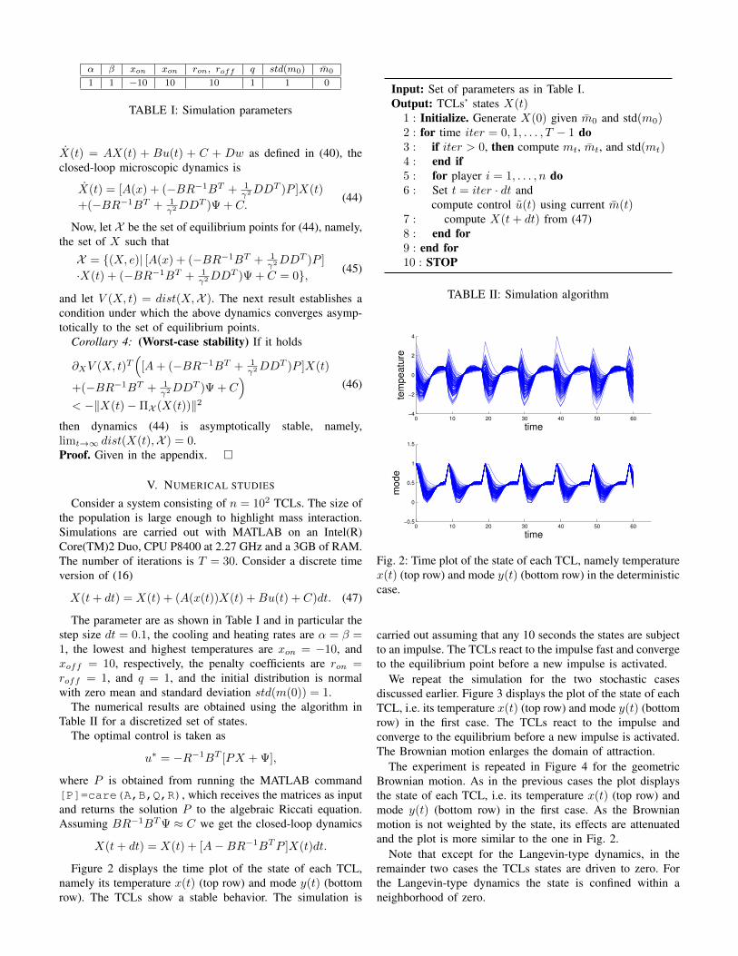
Figure 2 displays the time plot of the state of each TCL,namely its temperature x(t) (top row) and mode y(t) (bottomrow). The TCLs show a stable behavior. The simulation is

Input: Set of parameters as in Table I.Output: TCLs’ states X(t)

1 : Initialize. Generate X(0) given m0 and std(m0)2 : for time iter = 0, 1, . . . , T − 1 do3 : if iter > 0, then compute mt, mt, and std(mt)4 : end if5 : for player i = 1, . . . , n do6 : Set t = iter · dt and

compute control u(t) using current m(t)7 : compute X(t+ dt) from (47)8 : end for9 : end for10 : STOP

TABLE II: Simulation algorithm

0 10 20 30 40 50 60−4

−2

0

2

4

tem

peatu

re

time

0 10 20 30 40 50 60−0.5

0

0.5

1

1.5

mode

time

Fig. 2: Time plot of the state of each TCL, namely temperaturex(t) (top row) and mode y(t) (bottom row) in the deterministiccase.

carried out assuming that any 10 seconds the states are subjectto an impulse. The TCLs react to the impulse fast and convergeto the equilibrium point before a new impulse is activated.

We repeat the simulation for the two stochastic casesdiscussed earlier. Figure 3 displays the plot of the state of eachTCL, i.e. its temperature x(t) (top row) and mode y(t) (bottomrow) in the first case. The TCLs react to the impulse andconverge to the equilibrium before a new impulse is activated.The Brownian motion enlarges the domain of attraction.

The experiment is repeated in Figure 4 for the geometricBrownian motion. As in the previous cases the plot displaysthe state of each TCL, i.e. its temperature x(t) (top row) andmode y(t) (bottom row) in the first case. As the Brownianmotion is not weighted by the state, its effects are attenuatedand the plot is more similar to the one in Fig. 2.

Note that except for the Langevin-type dynamics, in theremainder two cases the TCLs states are driven to zero. Forthe Langevin-type dynamics the state is confined within aneighborhood of zero.

0 10 20 30 40 50 60−4

−2

0

2

4te

mpeatu

re

time

0 10 20 30 40 50 60−0.5

0

0.5

1

1.5

mode

time

Fig. 3: Time plot of temperature x(t) (top row) and modey(t) (bottom row) of each TCL in the stochastic case withstate dependent variance.

0 10 20 30 40 50 60−4

−2

0

2

4

tem

peatu

re

time

0 10 20 30 40 50 60−0.5

0

0.5

1

1.5

mode

time

Fig. 4: Time plot of temperature x(t) (top row) and modey(t) (bottom row) of each TCL in the stochastic case withstate independent variance.

VI. DISCUSSION

The topic of dynamic response has sparked attention fromdifferent disciplines. This is witnessed by the rapid growingof publications in different areas, from differential games [4],[11] to control and optimization [2], [10], [21], [22], [23], tocomputer science [26]. Actually, dynamic response intersectsresearch programs in smart buildings and smart cities. Theproblem is relevant due to an increasing size of the systemsand the consequent difficulties arising when centralizing themanagement.

The results of this paper are relevant for the followingreasons. First, the game-theoretic approach presented here is anatural way to deal with large scale, distributed systems whereno central planner can process all the information data. Oneway to deal with this issue, which is the main idea of dynamicdemand, aims at assigning part of the regulation burden to

the consumers by using frequency responsive appliances. Inother words, each appliance regulates automatically and in adecentralized fashion its power demand based on the mainsfrequency. In this respect, the provided model builds uponthe strategic interaction among the electrical appliances. Themodel suits the case where the appliances are numerous andindistinguishable. Indistinguishable means that any appliancein the same condition will react in the same way. Indistin-guishability is not a limitation, as in the case of heterogeneityof the electrical appliances, multi-population models may bederived based on the same approach used here.

The results provided in this paper shed light on the exis-tence of mean-field equilibrium solutions. By this we meanstrategies based on the forecasted demand, which attenuatemains frequency oscillations. Such strategies are stochastic,namely the TCL sets a probability with which to switch onor off . Stochastic linear strategies are designed as closed-loop strategies on the current state, temperature and switchingmode. Such strategies are computed over a finite horizon andtherefore are based on forecasted demand. The mean-fieldequilibrium strategies represent the asymptotic limit of Nashequilibrium strategies, and as such they are the best-responsestrategies of each player, for fixed behavior of the otherplayers. The proven stability of the microscopic dynamicsconfirms the asymptotic convergence of the TCLs’s states toan equilibrium, in terms of temperature and switching mode.The cases studied in the paper have shown that the strategiesare robust as convergence occurs also with imperfect models.In the case of imperfect modeling, model misspecifications areconsidered both in a stochastic and deterministic scenario.

VII. CONCLUDING REMARKS

We have developed a model based on mean-field gamesfor a population of thermostatically controlled loads. Themodel integrates both stochastic or deterministic disturbances.We have studied robust equilibria and designed stabilizingstochastic control strategies.

Within the realm of mean-field games, we can extend ourstudy in at least three directions. These include i) the analysisof the interplay between dynamic pricing and demand re-sponse, ii) the study of the benefits associated with coalitionalaggregation of a large number of power producers, and iii) thedesign of incentives to stabilize aggregation of producers.

APPENDIX

Proof of Theorem 1Let us start by isolating the HJI part of (13). For fixed mt

and for t ∈ [0, T ], we have

−∂tv(x, y, t)−{y[− α(x− xon)

]+(1− y)

[− β(x− xoff )

]}∂xv(x, y, t)

+ supu∈R

{−Bu∂yv(x, y, t)− 1

2qx2

+ 12u

T ru+ y(Se+W )}

= 0

in S×]0, T ],v(x, y, T ) = g(x) in S,

u∗(x, t) = −r−1BT∂yv(x, y, t),

(48)

which in a more compact form can be rewritten as

−∂tv(X, t)− supu

{∂Xv(X, t)T (AX +Bu+ C)

+ 12

(XTQX + uTRuT

)+ LTX

}= 0, in S × [0, T [,

v(X,T ) = g(X) in S,

u∗(x, t) = −r−1BT∂yv(X, t).


v(X, t) =1


and the corresponding optimal closed-loop state feedbackstrategy

u∗ = −R−1BT [PX + Ψ].

Then (48) can be rewritten as

12X

T P (t)X + Ψ(t)X + χ(t)

+(P (t)X + Ψ(t))T[−BR−1BT

]·(P (t)X + Ψ(t))

+(P (t)X + Ψ(t))T (AX + C)

+ 12


)+LTX(t) = 0 in S × [0, T [,

P (T ) = φ, Ψ(T ) = 0, χ(T ) = 0.

(49)


v(X,T ) =1


1

2XTφX =: g(X).

Since (49) is an identity in X , it reduces to three equations:

P + PA(x) +A(x)TP − PBR−1BTP+Q = 0 in [0, T [, P (T ) = φ,

Ψ +A(x)TΨ + PC − PBR−1BTΨ + L = 0in [0, T [, Ψ(T ) = 0,χ+ ΨTC − 1

2ΨTBR−1BTΨ = 0in [0, T [, χ(T ) = 0.

(50)

To understand the influence of the congestion term on thevalue function, let us develop the expression for Ψ and obtain

[Ψ1

Ψ2

]+

[−β 0

k(x(t)) 0

] [Ψ1

Ψ2

]+

[P11 P12

P21 P22

] [βxoff

0

]−[P12(r−1

on + r−1off )Ψ2

P22(r−1on + r−1

off )Ψ2

]+

[0

Se+W

].

(51)

The expression of Ψ then can be rewritten asΨ1 − βΨ1 + P11βxoff−P12(r−1

on + r−1off )Ψ2 = 0,

Ψ2 + k(x(t))Ψ1 − P22(r−1on + r−1

off )Ψ2

+(Se+W ) = 0,

(52)

which is of the form{Ψ1 + aΨ1 + bΨ2 + c = 0,

Ψ2 + a′Ψ1 + b′Ψ2 + c′ = 0.(53)

From the above set of inequalities, we obtain the solutionΨ(x(t), e(t), t). Note that the term a′ depends on x and c′

depends on e(t).Substituting the expression of the mean-field equilibrium

strategies u∗ = −R−1BT [PX+Ψ] as in (19) in the open-loopmicroscopic dynamics X(t) = AX(t)+Bu(t)+C introducedin (16), and averaging both LHS and RHS we obtain thefollowing closed-loop macroscopic dynamics

˙X(t) = [A(x)−BR−1BTP ]X(t)−BR−1BT Ψ(t) + C,

where Ψ(t) =∫ xoff

xon

∫[0,1]

Ψ(x, e, t)m(x, y, t)dxdy and thisconcludes our proof.

Proof of Corollary 1

Let X(t) be a solution of dynamics (20) with initial valueX(0) 6∈ X . Set t = {inf t > 0|X(t) ∈ X} ≤ ∞. For allt ∈ [0, t]

V (X(t+ dt))− V (X(t))= 1‖X(t)+dX(t)−ΠX (X(t))‖‖X(t) + dX(t)−ΠX (X(t))‖2

− 1‖X(t)−ΠX (X(t))‖‖X(t)−ΠX (X(t))‖2.

Taking the limit of the difference above we obtain

V (X(t)) = limdt→0V (X(t+dt))−V (X(t))

dt

= limdt→01dt

[1

‖X(t)+dX(t)−ΠX (X(t))‖‖X(t) + dX(t)

−ΠX (X(t))‖2

− 1‖X(t)−ΠX (X(t))‖‖X(t)−ΠX (X(t))‖2

]≤ 1‖X(t)−ΠX (X(t))‖

[∂XV (X, t)T

([A−BR−1BTP ]X(t)

−BR−1BTΨ + C)

+ ‖X(t)−ΠX (X(t))‖2]< 0,

which implies V (X(t)) < 0, for all X(t) 6∈ X and thisconcludes our proof.

Proof of Theorem 2

This proof follows the same reasoning as the proof ofTheorem 1. However, differently from there, here for thequadratic terms in (23) we have

σ11(x)2P11(t)+σ22(y)2P22(t) = σ211x

2P11(t)+σ222y

2P22(t).

Reviewing (23) as an identity in x, this leads to the followingthree equations to solve in the variable P (t), Ψ(t), and χ(t):

P (t) + P (t)A+ATP − PBR−1BTP +Q

+P = 0 in [0, T [, P (T ) = φ,


2ΨTBR−1BTΨ = 0in [0, T [, χ(T ) = 0,

(54)

where

P = Diag((σ2iiPii)i=1,2) =

[σ2

11P11 00 σ2

22P22

]. (55)


Let X(t) be a solution of dynamics (29) with initial valueX(0) 6∈ X . Set t = {inf t > 0|X(t) ∈ X} ≤ ∞ and letV (X(t)) = dist(X(t),X ). For all t ∈ [0, t]

V (X(t+ dt))− V (X(t)) = ‖X(t+ dt)−ΠX (X(t))‖−‖X(t)−ΠX (X(t))‖= 1‖X(t)+dX(t)−ΠX (X(t))‖‖X(t) + dX(t)−ΠX (X(t))‖2−

1‖X(t)−ΠX (X(t))‖‖X(t)−ΠX (X(t))‖2.

From the definition of infinitesimal generator

LV (X(t)) = limdt→0EV (X(t+dt))−V (X(t))

dt

≤ 1‖X(t)−ΠX (X(t))‖

[∂XV (X, t)T


−BR−1BTΨ + C)

+ 12 (σ2

11(x)∂xxV (X, t) + σ222(y)∂yyV (X, t))

].

From (31) the above implies that LV (X(t)) < 0, for allX(t) 6∈ M and this concludes our proof.

Proof of Theorem 3

From (32), in the HJB equation (23) we now have constantterms

1

2

2∑i=1

σii(.)2Pii(t) = σ2

11P11(t) + σ222P22(t).

Again, since the HJB equation (23) is an identity in x, itreduces to three equations:

P (t) + P (t)A+ATP − PBR−1BTP+Q = 0 in [0, T [, P (T ) = φ,


2ΨTBR−1BTΨ

+P = 0 in [0, T [, χ(T ) = 0,

(56)

whereP =

[σ2

11 00 σ2

22

]. (57)

Substituting the expression of the mean-field equilibriumstrategy u∗ = −R−1BT [PX+ Ψ] as in (36) in the open-loopmicroscopic dynamics dX(t) = (AX(t) + Bu(t) + C)dt +ΣdBt given in (22) and averaging both LHS and RHS weobtain the following closed-loop macroscopic dynamics

˙X(t) = [A−BR−1BTP ]X(t)−BR−1BTΨ(X(t)) + C,

and this concludes our proof.

A. Proof of Corollary 3

Let X(t) be a solution of dynamics (37) with initial valueX(0) 6∈ X . Set t = {inf t > 0|X(t) ∈ X} ≤ ∞ and letV (X(t)) = dist(X(t),X ). For all t ∈ [0, t]

V (X(t+ dt))− V (X(t)) = ‖X(t+ dt)−ΠX (X(t))‖−‖X(t)−ΠX (X(t))‖= 1‖X(t)+dX(t)−ΠX (X(t))‖‖X(t) + dX(t)−ΠX (X(t))‖2−

1‖X(t)−ΠX (X(t))‖‖X(t)−ΠX (X(t))‖2

From the definition of infinitesimal generator

LV (X(t)) = limdt→0EV (X(t+dt))−V (X(t))

dt

= limdt→01dt

[E(

1‖X(t)+dX(t)−ΠX (X(t))‖

‖X(t) + dX(t)−ΠX (X(t))‖2)

− 1‖X(t)−ΠX (X(t))‖‖X(t)−ΠX (X(t))‖2

]≤ 1‖X(t)−ΠX (X(t))‖

[∂XV (X, t)T


−BR−1BTΨ + C)

+ 12 (σ2

11∂xxV (X, t) + σ222∂yyV (X, t))

].

From (39) the above implies that LV (X(t)) < 0, for allX(t) 6∈ M and this concludes our proof.

Proof of Theorem 4

Isolating the HJI equation in (13), we have

−∂tVt(X)− supu infw

{∂XVt(X)T (AX +Bu

+C +Dw) + 12

(X(t)TQX(t)

+u(t)TRu(t)− γ2w(t)Tw(t))

+ LTX(t)}

= 0,

in S × [0, T [,

VT (X) = g(X) in S.

(58)


v(X, t) =1


and the corresponding mean-field equilibrium control andworst-case disturbance

u∗ = −R−1BT [PX + Ψ],w∗ = 1

γ2DT [PX + Ψ].

Then (58) can be rewritten as

12X

T P (t)X + Ψ(t)X + χ(t)

+(P (t)X + Ψ(t))T[−BR−1BT + 1

γ2DDT]

·(P (t)x+ Ψ(t)) + (P (t)x+ Ψ(t))T (AX + C)

+ 12

(X(t)TQX(t) + u(t)TRu(t)− γ2w(t)Tw(t)

)+LTX(t) + 1

2

∑2i=1 σii(.)

2Pii(t) = 0in R2 × [0, T [,

P (T ) = φ, Ψ(T ) = 0, χ(T ) = 0.


v(X,T ) =1


1

2XTφX =: g(X).

The above set of identities in x yields the following threeequations in the variable P (t), Ψ(t), and χ(t):

P (t) + P (t)A+ATP + P (−BR−1BT

+ 1γ2DD

T )P +Q = 0 in [0, T [, P (T ) = φ,

Ψ(t) +ATΨ + PC + (−BR−1BT

+ 1γ2DD

T )Ψ + L = 0 in [0, T [, Ψ(T ) = 0,

χ(t) + Ψ(t)TC + 12ΨT (−BR−1BT

+ 1γ2DD

T )Ψ = 0 in [0, T [, χ(T ) = 0.

(59)

Substituting the expressions of the mean-field equilibriumstrategies u∗ = −R−1BT [PX+Ψ] and w∗ = 1

γ2DT [PX+Ψ]

as in (43) in the open-loop microscopic dynamics X(t) =AX(t) + Bu(t) + C introduced in (40), and averaging bothLHS and RHS we obtain the following closed-loop macro-scopic dynamics

˙X(t) = [A+ (−BR−1BT + 1γ2DD

T )P ]X(t)


T )Ψ(X(t)) + C,(60)

and this concludes our proof.


Let X(t) be a solution of dynamics (44) with initial valueX(0) 6= X . Set t = {inf t > 0|X(t) ∈ X} ≤ ∞ and letV (X(t)) = dist(X(t),X ). For all t ∈ [0, t]

V (X(t+ dt))− V (X(t)) = ‖X(t+ dt)−ΠX (X(t))‖−‖X(t)−ΠX (X(t))‖= 1‖X(t)+dX(t)−ΠX (X(t))‖‖X(t) + dX(t)−ΠX (X(t))‖2

− 1‖X(t)−ΠX (X(t))‖‖X(t)−ΠX (X(t))‖2.

Using the asymptotic limit to differentiate the distance we have

V (X(t)) = limdt→0V (X(t+dt))−V (X(t))

dt

≤ 1‖X(t)−ΠX (X(t))‖

[∂XV (X, t)T

([A+ (−BR−1BT

+ 1γ2DD

T )P ]X(t)


T )Ψ + C)≤ 0

which implies V (X(t)) < 0, for all X(t) 6= X and thisconcludes our proof.

REFERENCES

[1] M. H. Albadi, E. F. El-Saadany, Demand Response in ElectricityMarkets: An Overview, IEEE, 2007.

[2] D. Angeli, P.-A. Kountouriotis, “A Stochastic Approach to Dynamic-Demand Refrigerator Control”, IEEE Transactions on Control SystemsTechnology, vol. 20, no. 3, pp. 581–592, 2012.

[3] F. Bagagiolo, D. Bauso, “Objective function design for robust optimal-ity of linear control under state-constraints and uncertainty”, ESAIM:Control, Optim. and Calculus of Variations, vol. 17, pp. 155–177, 2011.

[4] F. Bagagiolo, D. Bauso, “Mean-field games and dynamic demandmanagement in power grids”, Dynamic Games and Applications, vol.4, no. 2, pp. 155–176, 2014.

[5] M. Bardi, “Explicit solutions of some Linear-Quadratic Mean FieldGames”, Network and Heterogeneous Media, vol. 7, pp. 243–261, 2012.

[6] T. Basar, G. J. Olsder, Dynamic Noncooperative Game Theory, SIAMSeries in Classics in Applied Mathematics, Philadelphia, 1999.

[7] D. Bauso, Game Theory with Engineering Applications, SIAM’s Ad-vances in Design and Control series, Philadelphia, PA, USA, 2016.

[8] D. Bauso, T. Mylvaganam, A. Astolfi, “Crowd-averse robust mean-fieldgames: approximation via state space extension”, IEEE Transaction onAutomatic Control, vol. 61, no. 7, pp. 1882–1894, 2016.

[9] D. Bauso, H. Tembine, T. Basar, “Robust Mean Field Games”, Dyn.Games and Appl., vol. 6, no. 3, pp. 277–303, 2016.

[10] D. S. Callaway, I. A. Hiskens, “Achieving Controllability of ElectricLoads”, Proceedings of the IEEE, vol. 99, no. 1, pp. 184–199, 2011.

[11] R. Couillet, S.M. Perlaza, H. Tembine, M. Debbah, “Electrical Vehiclesin the Smart Grid: A Mean Field Game Analysis”, IEEE Journal onSelected Areas in Communications, vol. 30. no. 6, pp. 1086–1096, 2012.

[12] J. H. Eto, J. Nelson-Hoffman, C. Torres, S. Hirth, B. Yinger, J. Kueck,B. Kirby, C. Bernier, R.Wright, A. Barat, and D. S.Watson, “DemandResponse Spinning Reserve Demonstration,” Ernest Orlando LawrenceBerkeley Nat. Lab., Berkeley, CA, LBNL- 62761, 2007.

[13] C. Gellings, J. Chamberlin, Demand-Side Management: Concepts andMethods. Lilburn, GA: The Fairmont Press, 1988.

[14] D.A. Gomes, J. Saude, “Mean Field Games Models - A Brief Survey”,Dynamic Games and Applications, vol. 4, no, 2, pp. 110-154, 2014.

[15] O. Gueant, J. M. Lasry, P. L. Lions, “Mean-field games and applica-tions”, Paris-Princeton Lectures, Springer, pp. 1–66, 2010.

[16] M.Y. Huang, P.E. Caines, R.P. Malhame, “Individual and Mass Be-haviour in Large Population Stochastic Wireless Power Control Prob-lems: Centralized and Nash Equilibrium Solutions”, IEEE Conferenceon Decision and Control, HI, USA, December, pp. 98–103, 2003.

[17] M.Y. Huang, P.E. Caines, R.P. Malhame, “Large Population StochasticDynamic Games: Closed Loop Kean-Vlasov Systems and the NashCertainty Equivalence Principle”, Communications in Information andSystems, vol. 6, no. 3, pp. 221–252, 2006.

[18] M.Y. Huang, P.E. Caines, R.P. Malhame, “Large population cost-coupledLQG problems with non-uniform agents: individual-mass behaviourand decentralized ε-Nash equilibria”, IEEE Transactions on AutomaticControl, vol. 52. no. 9, pp. 1560–1571, 2007.

[19] J.-M. Lasry, P.-L. Lions, “Mean field games”, Japanese Journal ofMathematics, vol. 2, pp. 229–260, 2007.

[20] K. A. Loparo, X. Feng, “Stability of stochastic systems”. The ControlHandbook, CRC Press, pp. 1105-1126, 1996.

[21] Z. Ma, D. S. Callaway, I. A. Hiskens, “Decentralized Charging Controlof Large Populations of Plug-in Electric Vehicles”, IEEE Transactionson Control System Technology, vol. 21, no.1, pp. 67–78, 2013.

[22] J. L. Mathieu, S. Koch, D. S. Callaway, “State Estimation and Controlof Electric Loads to Manage Real-Time Energy Imbalance”, IEEETransactions on Power Systems, vol. 28, no.1, pp. 430–440, 2013.

[23] M. Roozbehani, M. A. Dahleh, S. K. Mitter, “Volatility of Power GridsUnder Real-Time Pricing”, IEEE Trans. on Power Syst., vol. 27, no. 4,2012.

[24] M. Sassano, A. Astolfi, “Dynamic Approximate Solutions of the HJInequality and of the HJB Equation for Input-Affine Nonlinear Systems”,IEEE Trans. on Automatic Control, vol. 57, no. 10, pp. 2490–2503, 2012.

[25] M. Sassano, A. Astolfi, “Approximate finite-horizon optimal controlwithout PDEs”, Systems & Control Letters, vol. 62 pp. 97–103, 2013.

[26] S. Esmaeil Zadeh Soudjani, S. Gerwinn, C. Ellen, M. Fraenzle, A. Abate,“Formal Synthesis and Validation of Inhomogeneous ThermostaticallyControlled Loads”, Quantitative Evaluation of Systems, Springer Verlag,pp.74–89, 2014.

[27] H. Tembine, Q. Zhu, and T. Basar, “Risk-sensitive mean-field games,”IEEE Trans. on Automatic Control, vol. 59, no. 4, pp. 835–850, 2014.

[28] US Department of Energy, Benefits of Demand Response in ElectricityMarkets and Recommendations for Achieving Them, Report to theUnited States Congress, February 2006. http://eetd.lbl.gov

[29] A. C. Kizilkale, R. P. Malhame, “Mean field based control of powersystem dispersed energy storage devices for peak load relief”, Proc. ofthe IEEE Conf. on Decision and Control (CDC), pp. 4971–4976, 2013.

[30] A. C. Kizilkale, R. P. Malhame, “Collective Target Tracking Mean FieldControl for Markovian Jump-Driven Models of Electric Water HeatingLoads”, Proc. of the 19th IFAC World Congress, Cape Town, SouthAfrica, pp. 1867–1872, 2014.

[31] M. Aziz, P. E. Caines, “A Mean Field Game Computational Methodol-ogy for Decentralized Cellular Network Optimization”, IEEE Trans. onControl Systems Technology, vol. 25, no. 2, pp. 563–576, 2017.

Dario Bauso received his Laurea degree in Aero-nautical Engineering in 2000 and his Ph.D. degreein Automatic Control and Systems Theory in 2004from the University of Palermo, Italy. Since 2015he has been with the Department of AutomaticControl and Systems Engineering, The Universityof Sheffield (UK), where he is currently Reader inControl and Systems Engineering. Since 2005 he hasalso been with the Dipartimento di Ingegneria Chim-ica, Gestionale, Informatica, Meccanica, Universityof Palermo (Italy), where he is currently Associate

Professor of Operations Research. From 2012 to 2014 he was also researchfellow at the Department of Mathematics, University of Trento (Italy).

His research interests are in the field of Optimization, Optimal andDistributed Control, and Game Theory. Since 2010 he is member of theConference Editorial Board of the IEEE Control Systems Society. He wasAssociate Editor of IEEE Transactions on Automatic Control from 2011 to2016. He is Associate Editor of Automatica, IEEE Control Systems Letters,and Dynamic Games and Applications.

dynamic demand and mean-ﬁeld games

Documents