dynamic factor models with infinite-dimensional factor space ... · with infinite-dimensional...
TRANSCRIPT

ECARES ULB - CP 114/04
50, F.D. Roosevelt Ave., B-1050 Brussels BELGIUM www.ecares.org
Dynamic Factor Models with Infinite-Dimensional Factor Space:
Asymptotic Analysis
Mario Forni
Università di Modena e Reggio Emilia, CEPR and RECent
Marc Hallin SBS-EM, ECARES, Université libre de Bruxelles
Marco Lippi
Einaudi Institute for Economics and Finance
Paolo Zaffaroni Imperial College and Università di Roma La Sapienza
June 2015
ECARES working paper 2015-23

Dynamic Factor Models with
Infinite-Dimensional Factor Space:
Asymptotic Analysis∗
Mario Forni†
Universita di Modena e Reggio Emilia, CEPR and RECent
Marc Hallin‡§
ECARES, Universite Libre de Bruxelles and ORFE, Princeton University
Marco Lippi¶
Einaudi Institute for Economics and Finance, Roma
Paolo Zaffaroni‖
Imperial College London and Universita di Roma La Sapienza
May 15, 2015
∗We are grateful to Michael Eichler and Giovanni Motta for suggestions and constructive criticism
on early versions of this research, and to Wei Biao Wu for helping us with crucial issues in multivariate
spectral estimation.†Research supported by the PRIN-MIUR Grant 2010J3LZEN.‡Research supported by an Interuniversity Attraction Pole (2012-2017) of the Belgian Science Policy
Office, a Credit aux Chercheurs of the Fonds de la Recherche Scientifique-FNRS of the Communautefrancaise de Belgique, and the Australian Research Council grant DP150100210.§Academie Royale de Belgique and CentER, Tilburg University.¶Research supported by the PRIN-MIUR Grant 2010J3LZEN.‖Research supported by the ESRC Grant RES-000-22-3219.
1

Abstract. Factor models, all particular cases of the Generalized Dynamic Factor Model
(GDFM) introduced in Forni, Hallin, Lippi and Reichlin (2000), have become extremely
popular in the theory and practice of large panels of time series data. The asymptotic prop-
erties (consistency and rates) of the corresponding estimators have been studied in Forni,
Hallin, Lippi and Reichlin (2004). Those estimators, however, rely on Brillinger’s dynamic
principal components, and thus involve two-sided filters, which leads to rather poor fore-
casting performances. No such problem arises with estimators based on standard (static)
principal components, which have been dominant in this literature. On the other hand, the
consistency of those static estimators requires the assumption that the space spanned by the
factors has finite dimension, which severely restricts the generality afforded by the GDFM.
This paper derives the asymptotic properties of a semiparametric estimator of the loadings
and common shocks based on one-sided filters recently proposed by Forni, Hallin, Lippi and
Zaffaroni (2015). Consistency and exact rates of convergence are obtained for this estimator,
under a general class of GDFMs that does not require a finite-dimensional factor space. A
Monte Carlo experiment corroborates those theoretical results and demonstrates the excellent
performance of those estimators in out-of-sample forecasting.
JEL subject classification : C0, C01, E0.
Key words and phrases: High -dimensional time series. Generalized dynamic factor models.
Vector processes with singular spectral density. One-sided representations of dynamic factor
models. Consistency and rates.
1 Introduction
In the present paper, we provide consistency results and consistency rates for the estimators
recently proposed by Forni, Hallin, Lippi and Zaffaroni (2015) (hereafter, FHLZ) for the
Generalized Dynamic Factor Model (GDFM).
Let
{xit, 1 ≤ i ≤ n0, 1 ≤ t ≤ T0} (1.1)
be an observed (n0 × T0)-dimensional panel, namely, a n0-tuple of time series observed over
a time period of length T0. The GDFM, as introduced in Forni et al. (2000) and Forni and
2

Lippi (2001) consists in modeling that panel as a finite realization of a stochastic process of
the form {xit, i ∈ N, t ∈ Z}, that is, a countable number of stochastic processes {xit, t ∈ Z}
admitting a decomposition of the form
xit = χit + ξit = bi1(L)u1t + bi2(L)u2t + · · ·+ biq(L)uqt + ξit, i ∈ N, t ∈ Z, (1.2)
where ut = (u1t u2t · · · uqt)′ is unobservable q-dimensional orthonormal white noise and
the filters bif (L), i ∈ N, f = 1, . . . , q, are square-summable (L, as usual, stands for the lag
operator); the unobservable processes χit and ξit are called the common and idiosyncratic
components, respectively. Detailed assumptions on (1.2) are given below. Let us only recall
here that the idiosyncratic components ξit and the common shocks uft are mutually orthogo-
nal at any lead and lag, and that the idiosyncratic components are “weakly” cross-correlated
(cross-sectional orthogonality being an extreme case).
Much of the literature on Dynamic Factor Models is based on (1.2) under the assumption
that the space spanned by the stochastic variables χit, for t given and i ∈ N, is finite-
dimensional.1 Under that assumption, model (1.2) can be rewritten in the so-called static
representation
xit = λi1F1t + λi2F2t + · · ·+ λirFrt + ξit
Ft = (F1t . . . Frt)′ = N(L)ut.
(1.3)
Criteria to determine r consistently have been given in Bai and Ng (2002) and, more recently,
in Alessi et al. (2010), Onatski (2010), and Ahn and Horenstein (2013). The vectors Ft and
the loadings λij can be estimated consistently using the first r standard principal components,
see Stock and Watson (2002a,b), Bai and Ng (2002). Moreover, the second equation in (1.3)
is usually specified as a possibly singular VAR, so that (1.3) becomes
xit = λi1F1t + λi2F2t + · · ·+ λirFrt + ξit
D(L)Ft = (I−D1L−D2L2 − . . .−DpL
p)Ft = Kut,(1.4)
where the matrices Dj are r× r while K is r× q, r ≥ q. Under (1.4), Bai and Ng (2007) and
Amengual and Watson (2007) provide consistent criteria to determine q.
The assumption of a finite-dimensional factor space, however, is far from being innocuous.
For instance, (1.3) is so restrictive that even the very elementary model
xit = ai(1− αiL)−1ut + ξit, (1.5)
1The definition of χit obviously implies that this dimension does not depend on t.
3

where q = 1, ut is scalar white noise, and the coefficients αi are drawn from a uniform
distribution over the stationary region, is ruled out. In this case, the space spanned, for
given t, by the common components χit, i ∈ N, is easily seen to be infinite-dimensional unless
the αi’s take only a finite number of values.
The problem is that, in the absence of the finite-dimensionality assumption, estimation
of model (1.2) cannot be based on a finite number r of standard principal components. That
situation is the one studied in Forni et al. (2000), who are using q principal components in the
frequency domain (Brillinger’s dynamic principal components; see Brillinger (1981)) to esti-
mate the common components χit.2 However, their estimators involve the application of two-
sided filters acting on the observations xit, and hence perform poorly at the end/beginning
of the observation period. As a consequence, they are of little help for prediction.
In FHLZ, we show how one-sided estimators without the finite-dimensionality assumption
can be obtained, under the additional condition that the common components have a rational
spectral density, that is, each filter bif (L) in (1.2) is a ratio of polynomials in L:
χit =ci1(L)
di1(L)u1t +
ci2(L)
di2(L)u2t + · · ·+ ciq(L)
diq(L)uqt, i ∈ N, f = 1, 2, . . . , q, (1.6)
where
cif (L) = cif,0 + cif,1L+ . . .+ cif,s1Ls1 and dif (L) = dif,0 + dif,1L+ . . .+ dif,s2L
s2
(the degrees s1 and s2 of the polynomials are assumed to be independent of i and f for the
sake of simplicity).
Denote by xt, χχχt, ξξξt the infinite-dimensional column vectors with components xit, χit,
and ξit, respectively. Elaborating upon recent results by Anderson and Deistler (2008a, b),
FHLZ prove that, for generic values of the parameters cif,k and dif,k (i.e. apart from a lower-
dimensional subset in the parameter space, see FHLZ for details), the infinite-dimensional
idiosyncratic vector χχχt = (χ1t χ2t · · · χnt · · · )′ admits a unique autoregressive representation
2Criteria to determine q without assuming (1.3) or (1.4) are obtained in Hallin and Liska, 2007
and Onatski, 2009.
4

with block structure of the form
A1(L) 0 · · · 0 · · ·
0 A2(L) · · · 0
. . .
0 0 · · · Ak(L)...
. . .
χχχt =
R1
R2
...
Rk
...
ut, (1.7)
where Ak(L) is a (q+ 1)× (q+ 1) polynomial matrix with finite degree and Rk is (q+ 1)× q.
Denoting by A(L) and R the (infinite) matrices on the left- and right-hand sides of (1.7),
respectively, and letting Zt = A(L)xt, it follows that
Zt = Rut + A(L)ξξξt. (1.8)
Under the assumptions of the present paper, the term A(L)ξξξt is still idiosyncratic, so
that (1.8) is a static representation of the form (1.4), with D(L) = I. That static rep-
resentation can be estimated via traditional principal components, which does not require
two-sided filters.
FHLZ thus obtain one-sided estimators for the common components without imposing the
standard finite-dimension restriction. Moreover, the high-dimensional VAR (1.7) is obtained
by piecing tothether the low-dimensional matrices Ak(L), each one depending only on the
covariances of q + 1 common components. Therefore, no curse of dimensionality occurs with
the procedure. Estimation of the common components χit, the shocks ut and the filters bif (L)
is based on the sample analogues of representations (1.7) and (1.8):
(i) We start with a lag-window estimator of the spectral density matrix of the observed
vector xnt = (x1t x2t · · · xnt), call it ΣΣΣxn(θ).
(ii) Using the first q frequency domain principal components of ΣΣΣxn(θ), we construct an
estimator of the spectral density of χχχnt = (χ1t χ2t · · · χnt), call it ΣΣΣχn(θ). Estimators
of the autocovariances of χχχnt are then obtained from ΣΣΣχn(θ); call ΓΓΓχn,h the estimator
of the covariance between χχχnt and χχχn,t−h. Those ΓΓΓχn,h’s are used, in a traditional,
low-dimensional way, to construct the autoregressive estimators Ak(L).
(iii) Blockwise estimators of the variables Zjt are obtained by applying the finite-degree
filters Ak(L) to the observed variables xit, while inverting the same Ak(L)’s provides
5

estimators for the filters bif (L). Estimators for the shocks uft and the matrix Rk are
obtained by using the first q traditional principal components of the variables Zit.
Our consistency results for the estimators described in (ii) and (iii) above are based
on recent results on lag-window spectral estimators in Shao and Wu (2007) and Liu and
Wu (2010), as extended to the multivariate case by Wu and Zaffaroni (2015). Starting with
the observable time series xit, denoting by T the number of observations for each series
and by σij(θ) a lag-window estimator of the cross-spectrum between xit and xjt, the (i, j)
entry of ΣΣΣ(θ), under quite general assumptions on the processes xit, xjt and the kernel,
these papers prove that σij(θ) is consistent, as T → ∞, uniformly with respect to θ, with
rate√BT logBT /T , where BT is the size of the lag window. As an important innovation with
respect to the previous literature on spectral estimation, these results are obtained without
assuming linearity or Gaussianity of the processes xit.
Using of those results here, however, requires some enhancement of the FHLZ assumptions
on the common shocks and the idiosyncratic components. In particular, the vector ut, which
is second-order white noise in FHLZ, is i.i.d. here. This, as well as some other changes
in the FHLZ assumptions, is discussed in detail in Section 2. Under this enhanced set of
assumptions, we prove that the estimators ΣΣΣχ(θ), ΓΓΓχ and Ak(L) are consistent with rate
ζnT = max(√
n−1,√T−1BT logBT
), (1.9)
where BT diverges as T δ, with 1/3 < δ < 1. Establishing those rates, raises some nontrivial
difficulties. Although model (1.8) is finite-dimensional, indeed, the series Zit are estimated,
not observed. As a consequence, the well-known results from static-factor literature (Stock
and Watson, 2002a and b, Bai and Ng, 2002) do not readily apply, and proving that consis-
tency holds with the same rates ζnT as if Zit were observed requires non negligible efforts.
As pointed out in FHLZ (end of Section 4.5) despite the fact that the dynamic model
studied in this paper is more general than model (1.4), when a dataset is given, with finite n
and T , the static approach might perform well even though the required finite-dimension
assumptions are not satisfied. A Monte Carlo study is provided in Section 4, in which the
static and dynamic methods have been applied to simulated data. A very short summary of
our results is that (i) when the data are generated by infinite-dimensional models which are
simple generalizations of (1.5), the estimation of impulse-response functions and predictions
6

via the dynamic method is by far better than those obtained via the static one; (ii) even
when the data are generated by (1.4), still the dynamic method performs slightly better.
Though not conclusive, our Monte Carlo results strongly suggest that the model proposed in
the present paper may be uniformly competitive.
The paper is organized as follows. In Sections 2, we present and comment the main as-
sumptions to be made throughout. Section 3 provides the main asymptotic results. Section 4
gives a detailed description of the Monte Carlo experiments, and their analysis, and Section 5
concludes. Short proofs are given in the body of the paper, the longer ones in the Appendix.
2 Main assumptions and some preliminary results
2.1 Common and idiosyncratic components
The Dynamic Factor Model studied in the present paper is a decomposition, of the form
xit = χit + ξit, i ∈ N, t ∈ Z
of an observed variable xit into a nonobserved common component χit and a nonobserved
idiosyncratic component ξit. Throughout, we are assuming that the family of stochastic
variables
{xit, χit, ξit, i ∈ N, t ∈ Z},
fulfills the assumptions listed below as Assumptions 1 through 10.
Assumption 1 There exist a natural number q > 0 and
(1) a q-dimensional stochastic zero-mean process ut = (u1t u2t · · · uqt)′, t ∈ Z, and an
infinite-dimensional stochastic process ηηηt = (η1t η2t · · · )′, t ∈ Z;
(2) square-summable filters bif (L), i ∈ N, f = 1, . . . , q;
(3) coefficients βij,k, for i, j ∈ N, k = 0, 1, . . . ,∞, where∑∞
j=1
∑∞k=0 β
2ij,k < ∞ for all i ∈
N;
such that
7

(i) the vectors St = (u′t ηηη′t)′, t ∈ Z, are i.i.d. and orthonormal, i.e. E(StS
′t) = I∞; in
particular, cov(uft, ηj,t−k) = 0, f = 1, . . . , q, j ∈ N, k = 0, 1, . . . ,∞;
(ii) χit = bi1(L)u1t + bi2(L)u2t + · · ·+ biq(L)uqt
ξit =∞∑j=1
∞∑k=0
βij,kηj,t−k.(2.1)
Clearly, neither ut nor the polynomials bif (L) are identified. Indeed, rewriting the first
equation in (2.1) as χit = bi(L)ut, for any orthogonal matrix Q, the common component χit
has the alternative representation χit =[bi(L)Q−1
][Qut] = b∗i (L)u∗t . Note that (i) and (2.1)
imply cov(uft, ξi,t−k) = 0 for all f, i, k.
Two differences with respect to FHLZ must be pointed out. Firstly, here ut is i.i.d.,
not just second-order white noise as in FHLZ. Secondly, unlike in FHLZ, the idiosyncratic
components are modeled as (infinite-order) moving averages of the infinite-dimensional i.i.d.
vector ηηηt.
Assumption 2 Conditions on the filters bif (L).
(i) The filters bif (L) are rational. More precisely, there exist natural numbers s1, s2 such
that bif (L) = cif (L)/dif (L), where
cif (L) = cif,0 + cif,1L+ · · ·+ cif,s1Ls1 and dif (L) = 1 + dif,1L+ · · ·+ dif,s2L
s2 , (2.2)
for i ∈ N, f = 1, . . . , q.
(ii) There exists φ > 1 such that none of the roots of dif (L) is less than φ in modulus,
for i ∈ N, f = 1, . . . , q.
(iii) There exists Bχ, 0 < Bχ <∞, such that |cif,j | ≤ Bχ, i ∈ N, f = 1, . . . , q, j = 0, . . . , s1.
Under Assumption 2, the vector χχχnt = (χ1t χ2t · · · χnt)′ has a rational spectral density
matrix ΣΣΣχn(θ); denote by λχnj(θ) its j-th eigenvalue (in decreasing order).
Assumption 3 Common component spectral density eigenvalues: divergence and separation.
There exist continuous functions
αχf (θ), f = 1, . . . , q and βχf (θ), f = 0, . . . , q − 1, θ ∈ [−π, π],
8

and a positive integer nχ such that, for n > nχ,
βχ0 (θ) ≥ λχn1(θ)
n≥ αχ1 (θ) > βχ1 (θ) ≥ λχn2(θ)
n≥ · · · ≥ αχq−1(θ) > βχq−1(θ) ≥
λχnq(θ)
n≥ αχq (θ) > 0,
for all θ ∈ [−π, π].
Assumption 3 is an enhancement of the standard assumption on the eigenvalues of com-
mon components. It will be used in our consistency proof: see, in particular, Lemma 3,
Appendix B.
Assumption 4 Serial dependence of idiosyncratic components.
There exists finite positive numbers B, Bis, i ∈ N, s ∈ N, and ρ, 0 ≤ ρ < 1, such that
∞∑s=1
Bis ≤ B, for all i ∈ N (2.3)
∞∑i=1
Bis ≤ B, for all s ∈ N (2.4)
|βis,k| ≤ Bisρk, for all i, s ∈ N and k = 0, 1, . . . (2.5)
An immediate consequence of (2.3) and (2.4) is that
∞∑i=1
∞∑s=1
BisBjs ≤ B2, for all j ∈ N. (2.6)
Conditions (2.3) and (2.4) are quite obviously satisfied in the “purely idiosyncratic”
case ξit = ηit, and for finite “cross-sectional moving averages” such as ξit = ηit + ηi+1,t. By
condition (2.5), the time dependence of the variables ξit declines geometrically, at common
rate ρ.
Under Assumption 4, setting βis(L) =∑∞
k=0 βis,kLk and ξit =
∑∞s=1 βis(L)ηst, and de-
noting by ı the imaginary unit,
|βis(e−ıθ)| =
∣∣∣∣∣∞∑k=0
βis,ke−ıkθ
∣∣∣∣∣ ≤∞∑k=0
|βis,k| ≤∞∑k=0
Bisρk ≤ Bis
1
1− ρ.
Therefore, letting σξij(θ) be the cross-spectral density of ξit and ξjt,
∞∑i=1
|σξij(θ)| ≤1
2π
∞∑i=1
∞∑s=1
|βis(e−ıθ)βjs(e−ıθ)| ≤ 1
2π(1− ρ)2
∞∑i=1
∞∑s=1
BisBjs
≤ B2 1
2π(1− ρ)2,
(2.7)
9

by (2.6). Assumption 4 thus implies that the cross-spectra σξij(θ) are bounded, in θ, uniformly
in i and j. On the other hand, Assumption 2, (ii) and (iii), implies that σχij(θ) is bounded,
in θ, uniformly in i and j. Therefore, σxij(θ) = σχij(θ) +σξij(θ) is bounded, in θ, uniformly in i
and j.
The spectral density matrices of the ξ’s and the x’s, and their eigenvalues, ordered in
decreasing order, are denoted by ΣΣΣξn(θ), ΣΣΣx
n(θ), λξnj(θ) and λxnj(θ), respectively; under the
above assumptions, they satisfy the following properties.
Proposition 1 Under Assumptions 1 through 4,
(i) there exists Bξ > 0 such that λξn1(θ) ≤ Bξ for all n ∈ N and θ ∈ [−π, π] (thus, the ξ’s
are idiosyncratic, see FHLZ, Section 2.2);
(ii) there exists nx ∈ N such that, for n > nx and all θ ∈ [−π, π],
λxn1(θ)
n> αχ1 (θ) >
λxn2(θ)
n> · · · > αχq−1(θ) >
λxnq(θ)
n> αχq (θ),
where the functions αχj (θ) are defined in Assumption 3;
(iii) there exists Bx > 0 such that λxn,q+1(θ) ≤ Bx for all n ∈ N and θ ∈ [−π, π].
Proof. The column and row norms of ΣΣΣξn(θ) are equal, and, by (2.7), satisfy
maxj=1,2,...,n
n∑i=1
|σξij(θ)| ≤ maxj=1,2,...,n
∞∑i=1
|σξij(θ)| ≤ B2 1
2π(1− ρ)2.
On the other hand, the product of the row and the column norms, the square of the column
norm in our case, is greater than or equal to the square of the spectral norm, see Lancaster and
Tismenetsky (1985), p. 366, Exercise 11. As a consequence, setting Bξ = B21/2π(1− ρ)2,
we have λξn1(θ) ≤ Bξ for all n and θ.
Regarding (ii), ΣΣΣxn(θ) = ΣΣΣχ
n(θ) + ΣΣΣξn(θ) implies that
λxnf (θ) ≥ λχnf (θ) + λξnn(θ) and λxnf (θ) ≤ λχnf (θ) + λξn1(θ)
(these are two of the Weyl inequalities, see Franklin (2000), p. 157, Theorem 1; see also
Appendix B). By Assumption 3,
λxnf (θ)
n≥λχnf (θ) + λξnn(θ)
n> αχf (θ),
10

for f = 1, . . . , q, and, for f = 2, . . . , q,
λxnf (θ)
n≤λχnf (θ) + λξn1(θ)
n≤λχnf (θ)
n+Bξ
n≤ βχf−1(θ) +
Bξ
n< αχf−1(θ),
for n > nχ, nχ being such that Bξ/nχ < minf=1,2,...,q
[minθ∈[−π, π](α
χf (θ)− βχf (θ))
].
As for (iii), λxn,q+1 ≤ λχn,q+1(θ) + λξn1(θ). On the other hand, λχn,q+1(θ) = 0 for all θ. The
result then follows from (i). �
Proposition 2 Under Assumptions 1 through 4, the cross-spectral densities σxij(θ) possess
derivatives of any order and are of bounded variation uniformly in i, j ∈ N; namely, there
exists Ax > 0 such thatν∑h=1
|σxij(θh)− σxij(θh−1)| ≤ Ax
for all i, j, ν ∈ N and all partitions
−π = θ0 < θ1 < · · · < θν−1 < θν = π
of the interval [−π, π].
Proof. Denoting by γξij,h, h ≥ 0, the covariance between ξit and ξj,t−h,
|γξij,h| =
∣∣∣∣∣∞∑k=0
∞∑s=1
βis,kβjs,k+h
∣∣∣∣∣ ≤∞∑k=0
∞∑s=1
BisBjsρkρk+h ≤ ρh
∞∑k=0
ρ2k∞∑s=1
BisBjs ≤ ρhB2
1− ρ2,
(2.8)
by (2.6). For h < 0, γξij,h = γξji,−h, so that |γξij,h| ≤ ρ|h|B2/(1− ρ2). This implies that
σξij(θ) =1
2π
∞∑h=−∞
γξij,he−ıhθ
has derivatives of all orders. Moreover,∣∣∣∣ ddθσξij(θ)∣∣∣∣ =
1
2π
∣∣∣∣∣∞∑
h=−∞(−ıh)γξij,he
−ıhθ
∣∣∣∣∣ ≤ B2
π(1− ρ2)
∞∑h=1
hρh =B2ρ
π(1− ρ2)(1− ρ)2,
which entails bounded variation of σξij(θ) uniformly in i and j. Bounded variation of σχij(θ),
uniformly in i and j, is an obvious consequence of Assumption 2. The conclusion follows
from the fact that σxij(θ) = σχij(θ) + σξij(θ). �
11

2.2 Autoregressive representation of the χ’s
In FHLZ we prove that, for generic values of the parameters cif,k and dif,k in (2.2), the space
spanned by uf,t−k, f = 1, 2, . . . , q, k ≥ 0, is equal to the space spanned by any (q + 1)-
dimensional subvector of χχχt and its lags. In other words, ut is fundamental for all the (q+1)-
dimensional subvectors of χχχt (but not for all q-dimensional ones). Moreover, we prove that,
generically, the (q+ 1)-dimensional subvectors of χχχt admit a finite and unique autoregressive
representation (see, in particular, Section 4.1, Lemma 3). Following FHLZ, we use these
genericity results as a motivation for assuming that each of the vectors(χ1t χ2t · · · χq+1,t
),(χq+2,t χq+3,t · · · χ2(q+1),t
), . . . ,
that is, each of the vectors
χχχkt =(χ(k−1)(q+1)+1,t · · · χk(q+1),t
), k ∈ N,
and its lags spans the space spanned by the u’s and has a unique finite autoregressive repre-
sentation.
Assumption 5 Each vector χχχkt , k ∈ N, has an autoregressive representation
Ak(L)χχχkt = Rkut, (2.9)
where
(i) Ak is (q + 1)× (q + 1), of degree not greater than S = qs1 + q2s2, and Ak(0) = Iq+1;
(ii) Rk is (q + 1)× q and has rank q;
(iii) the representation (2.9) is unique among the autoregressive representations of order
not greater than S, i.e. if B(L)χχχkt = Rut, where the degree of B(L) does not exceed S
and B(0) = Iq+1, then B(L) = Ak(L) and R = Rk.
Representation (2.9) is a specification of (1.7) (the degrees of the polynomial matri-
ces Ak(L) and their uniqueness).3 Writing A(L) for the (infinite) block-diagonal matrix
3Based on a genericity argument, FHLZ assume that (2.9) holds for any (q+ 1)-dimensional vector
(χi1,t χi2,t · · · χiq+1,t), see Assumption A.3. The weaker version in Assumption 5 above is sufficient
for our purposes.
12

with diagonal blocks A1(L),A2(L), . . ., and letting R = (R1′,R2′, · · · )′, we thus have
A(L)χχχt = Rut. (2.10)
The upper n × n submatrix of A(L) and the upper n × q submatrix of R are denoted
by An(L) and Rn respectively. If n = m(q + 1), so that the first m blocks of size q + 1 are
included,
An(L)χχχnt = Rnut. (2.11)
The following proposition is an immediate consequence of the fact that (2.10) is the
difference between χχχt and its orthogonal projection on its past values; details are left to the
reader.
Proposition 3 Let Assumptions 1 through 5 hold.
(i) Let A∗(L)χχχt = R∗vt, where the degree of A∗(L) is at most S: then, A∗(L) = A(L),
and there exists a q × q orthogonal matrix Q such that R∗ = RQ′ and vt = Qut.
(ii) Let r = (r1 · · · rq) be the row of R (the row of Rk) corresponding to χit: then,
rf = cif (0) = cif,0, f = 1, . . . , q, i ∈ N.
Letting ΨΨΨt = A(L)χχχt = Rut, denote by ΓΓΓψn the variance-covariance matrix of ΨΨΨnt, with
eigenvalues µψnj , j = 1, . . . , n, in decreasing order.
Assumption 6 There exist real numbers αψf , f = 1, . . . , q, βψf , f = 0, . . . , q − 1, and a
positive integer nψ such that, for n > nψ,
βψ0 ≥µψn1
n≥ αψ1 > βψ1 ≥
µψn2
n≥ αψ2 > βψ2 ≥ · · · ≥ α
ψq−1 > βψq−1 ≥
µψnqn≥ αψq > 0.
Note that the eigenvalues µψnf depend on the coefficients cif,0, see Proposition 3(ii), but
are invariant if R and ut are replaced by RQ′ and Qut respectively.
We now show how the matrices Ak(L) appearing in (2.9) can be constructed from the
spectral density of the χ’s. This construction, with the population quantities replaced by
their estimates, leads to our estimator as explained in Section 3. It proceeds in two steps:
(i) Denoting by ΣΣΣχjk(θ) the (q+ 1)× (q+ 1) cross-spectral density between χχχjt and χχχkt , and
by ΓΓΓχjk,s the covariance between χχχjt and χχχkt−s, we have
ΓΓΓχjk,s = E(χχχjtχχχ
kt−s′ )
=
∫ π
−πeısθΣΣΣχ
jk(θ)dθ. (2.12)
13

(ii) The minimum-lag matrix polynomial Ak(L) and the variance-covariance function of
the unobservable vectors
ΨΨΨ1t = A1(L)χχχ1
t , ΨΨΨ2t = A2(L)χχχ2
t . . . (2.13)
follow from that autocovariance function ΓΓΓχkk,s. Indeed, defining
Ak(L) = Iq+1 −Ak1L− · · · −Ak
SLS ,
A[k] =(Ak
1 Ak2 · · · Ak
S
), Bχ
k =(ΓΓΓχkk,1 ΓΓΓχkk,2 · · · ΓΓΓχkk,S
)(2.14)
and
Cχjk =
ΓΓΓχjk,0 ΓΓΓχjk,1 · · · ΓΓΓχjk,S−1
ΓΓΓχjk,−1 ΓΓΓχjk,0 · · · ΓΓΓχjk,S−2...
...
ΓΓΓχjk,−S+1 ΓΓΓχjk,−S+2 · · · ΓΓΓχjk,0
, (2.15)
we have
A[k] = Bχk
(Cχkk
)−1= Bχ
k
(Cχkk
)ad
det(Cχkk
)−1, (2.16)
where(Cχkk
)ad
stands for the adjoint of the square matrix Cχkk.
Non-singularity of Cχkk is necessary for the uniqueness of the A[k]’s, and it therefore is
implied by Assumption 5. However, we require a slightly stronger condition to ensure that
the A[k]’s are (uniformly) bounded, in norm, as n tends to infinity.
Assumption 7 There exists a real d > 0 such that∣∣det Cχ
kk
∣∣ > d for all k ∈ N.
For any fixed n and, in particular, for n = n0 (supposed to be a multiple of q + 1),
the existence of a constant dn > 0 such that∣∣det Cχ
kk
∣∣ > dn for 1 ≤ k ≤ n/(q + 1) is
a consequence of Assumption 5. Assumption 7, however, is more demanding, as it imposes∣∣det Cχkk
∣∣ > d for all k ∈ N and a d that does not depend on n. This is reasonable if we require
the (fictitious) “cross-sectional future” of the panel to resemble what has been observed, i.e.
the n0-dimensional panel (1.1)—a form of cross-sectional stationarity.
Letting Zt = A(L)xt, we have
Zt = ΨΨΨt + ΦΦΦt
with ΨΨΨt = Rut ΦΦΦt = A(L)ξξξt.(2.17)
14

Denote by ΓΓΓΦn the variance-covariance matrix of ΦΦΦnt = (Φ1t Φ2t · · · Φnt) and by µΦ
nj its j-th
eigenvalue: the following holds
Proposition 4 Under Assumptions 1 through 7, there exists BΦ > 0 such that µΦn1 ≤ BΦ
for all n ∈ N.
Proof. Let λΦnj(θ) be the j-th eigenvalue of the spectral density matrix of ΦΦΦnt. Let us show
that there exists a constant CΦ such that λΦn1(θ) ≤ CΦ for all n and θ. Because λΦ
n1(θ), for
all θ, is non-decreasing with n (see Forni and Lippi, 2001), we can assume without loss of
generality that n = m(q + 1). The spectral density of ΦΦΦnt is
An(e−ıθ)ΣΣΣξn(θ)A′n(eıθ),
where An(L) (see equation (2.11)) has the matrices Ak(L) on the diagonal. If a(θ) is an
n-dimensional complex column vector such that a(θ)′a(θ) = 1 for all θ, we have
a(θ)′An(e−ıθ)ΣΣΣξn(θ)A′n(eıθ)a(θ) ≤ λξn1(θ)
(a′(θ)An(e−ıθ)A′n(eıθ)a(θ)
)≤ λξn1(θ)λAn
1 (θ),
where λAn1 (θ) is the first eigenvalue of An(e−ıθ)A′n(eıθ), which is Hermitian, non-negative
definite. By Proposition 1 supn λξn1(θ) ≤ Bξ. Moreover, given the diagonal structure
of An(L), λAn1 (θ) = supk=1,2,...,m λ
Ak
1 (θ) ≤ supk∈N λAk
1 (θ), where λAk
1 (θ) is the first eigenvalue
of Ak(e−ıθ)Ak ′(eıθ). Assumptions 2 and 7 imply that supk∈N λAk
1 (θ) ≤ DΦ for some DΦ > 0
and all θ. On the other hand,
λΦn1(θ) = sup a(θ)′An(e−ıθ)ΣΣΣξ
n(θ)A′n(eıθ)a(θ) ≤ BξDΦ,
the sup being over all the vectors a(θ) such that a(θ)′a(θ) = 1. Lastly,
µΦn1 = sup b′ΓΓΓΦ
nb =
∫ π
−π
(b′ΣΣΣΦ
n (θ)b)dθ ≤
∫ π
−πλΦn1(θ)dθ ≤ 2πBξDΦ,
the sup being over all the n-dimensional column vectors b such that b′b = 1. �
Note that ΦΦΦt and ΨΨΨt are mutually orthogonal, a consequence of Assumption 1(i). In view
of Assumption 6 and Proposition 4, the model (2.17) is thus a static factor model—a special
case of (1.4), with r = q and N(L) = Iq.
15

3 Estimation: asymptotics
Our estimation procedure follows the same steps as the population construction in Section 2.2,
with the population spectral density of the x’s replaced with an estimator ΣΣΣxn(θ) fulfilling
Assumption 9 below. Based on Forni et al. (2000), we obtain the estimator ΣΣΣχn(θ) by means
of the first q frequency-domain principal components of the x’s (using the first q eigenvectors
of ΣΣΣxn(θ)). Then the matrices ΓΓΓχjk, Bχ
jk, Cχjk and An(L) are computed as natural counterparts
of their population versions in Section 2.2. Finally, estimators for Rn and ut are obtained
via a standard principal component analysis of Znt = A(L)xnt. Consistency with exact rate
of convergence ζnT , as defined in equation (1.9), for all the above estimators are provided in
Propositions 7 through 11.
Explicit dependence on the index n has been necessary in Section 2. From now on, it
will be convenient to introduce a minor change in notation, dropping n whenever possible.
In particular,
(i) ΣΣΣx(θ) =(σxij(θ)
)i,j=1,...,n
and λxf (θ) replace ΣΣΣxn(θ) and λxnf (θ), respectively.
(ii) ΛΛΛx(θ) denotes the q × q diagonal matrix with diagonal elements λxf (θ).
(iii) Px(θ) denotes the n×q matrix the q columns of which are the unit-modulus eigenvectors
corresponding to ΣΣΣx(θ)’s first q eigenvalues. The columns and entries of Px(θ) are
denoted by Pxf (θ) and pxif (θ), f = 1, . . . , q, i = 1, . . . , n, respectively.
(iv) ΣΣΣχ(θ) =(σχij(θ)
)i,j=1,...,n
, λχf (θ), ΛΛΛχ(θ), Pχ(θ), ΣΣΣξ(θ), etc. are defined as in (i).
(v) All the above matrices and scalars depend on n; the corresponding estimators,
ΣΣΣx(θ), λxf (θ), ΛΛΛx(θ), Px(θ) and ΣΣΣχ(θ), λχf (θ), ΛΛΛχ(θ), Pχ(θ)
(precise definitions are provided below) depend both on n and the observed values
xit, i = 1, . . . , n, t = 1, . . . , T . For simplicity, we say that they depend on n and T .
(vi) The same notational change applies to ΓΓΓψn and related eigenvalues and eigenvectors.
(vii) A(L) and R, denoting the upper left n × n and n × q submatrices of A(L) and R,
respectively, are used instead of An(L) and Rn; A(L) and R stand for their estimated
counterparts.
16

(viii) To avoid confusion, however, we keep explicit reference to n in xnt, χχχnt, Znt etc.,
with estimated counterparts of the form χχχnt, Znt, etc.; thus, we write, for instance,
Znt = A(L)xnt = Rut + ΦΦΦnt.
(ix) Lastly, if F is a matrix, we denote by F its conjugate transpose, and by ||F|| its spectral
norm (see Appendix B).
3.1 Estimation of ΣΣΣx(θ)
The following definition, coined by Wu (2005), generalizes the usual measures of time depen-
dence for stochastic processes.
Definition 1 Physical dependence. Let εεεt be an i.i.d. stochastic vector process, possibly
infinite-dimensional, and let zt = F (εεεt, εεεt−1, . . .), where F : [R×R×· · · ]→ R is a measurable
function; assume that zt has finite p moment for p > 0. Let εεε∗ be a stochastic vector with
the same dimension and distribution as the εεεt’s, such that εεε∗ and εεεt are independent for all t.
For k ≥ 0 the physical dependence δ[zt]kp is defined as
δ[zt]kp = (E (|F (εεεk, . . . , εεε0, εεε−1, . . .)− F (εεεk, . . . , εεε
∗, εεε−1, . . .)|p))1/p .
Assumption 8 There exist p, A, with p > 4, 0 < A <∞, such that
E (|uft|p) ≤ A, E (|ηit|p) ≤ A, (3.1)
for all i ∈ N and f = 1, . . . , q.
The main result of the section, that the estimate of the cross-spectral density between xit
and xjt converges uniformly with respect to the frequency and to i and j, see Proposition 6,
requires the following results on the p-th moments and the physical dependence of the x’s.
Proposition 5 Under Assumptions 1 through 8, there exist ρ1 ∈ (0, 1) and A1 ∈ (0,∞)
such that, for all i ∈ N,
E (|xit|p) ≤ A1 and δ[xit]kp ≤ A1ρ
k1. (3.2)
17

Proof. By the Minkovski inequality,
(E (|xit|p))1p = (E (|χit + ξit|p))
1p ≤ (E (|χit|p))
1p + (E (|ξit|p))
1p .
Using the Minkovski inequality again, condition (2.3) and Assumption 8, we obtain
(E (|ξit|p))1p =
(E
(∣∣∣∣∣∞∑s=1
∞∑k=0
βis,kηs,t−k
∣∣∣∣∣p)) 1
p
≤∞∑s=1
∞∑k=0
(E (|βis,kηs,t−k|)p)1p
≤∞∑s=1
∞∑k=0
|βis,k|E (|ηs,t−k|p)1p ≤ A
1p
∞∑s=1
∞∑k=0
Bisρk ≤ A
1pB
1
1− ρ.
An analogous inequality can be obtained for the common components, using Assumption 2
and the first of inequalities (3.1). The first inequality in (3.2) follows.
Turning to the second inequality, for k ≥ 0,
ξik − ξ∗ik =∞∑s=1
βis,k(ηsk − η∗s),
where ξ∗ik has the same definition as ξik, with ηs0 replaced by η∗s . The Minkovski inequality,
condition (2.3) and Assumption 8 imply
δ[ξit]k,p =
(E
(∣∣∣∣∣∞∑s=1
βis,k(ηsk − η∗s)
∣∣∣∣∣p)) 1
p
≤∞∑s=1
(E (|βis,k(ηsk − η∗s)|p))1p
≤ ρk∞∑s=1
Bis (E (|ηsk − η∗s)|p))1p ≤ ρk2BA
1p .
An analogous inequality can be ontained for the common components, using Assumption 2
and the first of inequalities (3.1), with ρ replaced by φ−1, φ being defined in Assumption 2.
Then,
δ[xit]kp = (E |xit − x∗it|p)
1p =
(E (|(χit − χ∗it) + (ξit − ξ∗it)|p)
1p
)≤ (E (|χit − χ∗it|)
p)1p + (E (|ξit − ξ∗it|)
p)1p = δ
[χit]kp + δ
[ξit]kp .
The conclusion follows. �
Consider now the lag-window estimator
ΣΣΣx(θ) =1
2π
T−1∑k=−T+1
K
(k
BT
)e−ıkθΓΓΓxk, (3.3)
of the spectral density ΣΣΣx(θ), where ΓΓΓxk = 1T∑T
t=|k|+1 xtxt−|k|.
18

Assumption 9 Lag-window estimation of ΣΣΣx(θ).
(i) The kernel function K is even, bounded, with support [−1, 1]; moreover,
(1) for some κ > 0, |K(u)− 1| = O(|u|κ) as u→ 0,
(2)∫∞−∞K
2(u)du <∞,
(3)∑
j∈Z sup|s−j|≤1 |K(jw)−K(sw)| = O(1) as w → 0;
(ii) For some c1, c2 > 0, δ and δ such that 0 < δ < δ < 1 < δ(2κ+ 1), c1Tδ ≤ BT ≤ c2T
δ.
Proposition 6 Under Assumptions 1 through 9, there exists C > 0 such that
E
(max|h|≤BT
∣∣σxij(θ∗h)− σxij(θ∗h)∣∣2) ≤ C (T−1BT logBT
), (3.4)
where θ∗h = πh/BT , for all T , i and j in N.
See Appendix A for the proof.
3.2 Estimation of σχij(θ) and γχij,k
Our estimator of the spectral density matrix of the common components χχχnt is the Forni
et al. (2000) estimator ΣΣΣχ(θ) = Px(θ)ΛΛΛx(θ) ˜Px(θh).
Proposition 7 Under Assumptions 1 through 7,
max|h|≤BT
|σχij(θ∗h)− σχij(θ
∗h)| = OP (ζnT ) ,
where θ∗h = πh/BT , as T → ∞ and n → ∞, uniformly in i and j. Precisely, for any ε > 0,
there exists η(ε), independent of i and j, such that, for all n and T ,
P
(maxh≤BT
|σχii(θ∗h)− σχii(θ∗h)|ζnT
≥ η(ε)
)< ε.
See Appendix B for the proof.
Our estimator of the covariance γχij,` of χit and χj,t−` is, as in Forni et al. (2005),
γχij,` =π
BT
∑|h|≤BT
eı`θ∗h σχij(θ∗h), (3.5)
where θ∗h = πh/BT . Recalling that γχij,` =∫ π−π e
ı`θσχij(θ)dθ, we have
19

|γχij,` − γχij,`| ≤
π
BT
∑|h|≤BT
|eı`θ∗h σχij(θ∗h)− eı`θ∗hσχij(θ
∗h)|
+
∣∣∣∣∣∣ πBT∑|h|≤BT
eı`θ∗hσχij(θ∗h)−
∫ π
−πeı`θσχij(θ)dθ
∣∣∣∣∣∣≤ π
BT
∑|h|≤BT
|σχij(θ∗h)− σχij(θ
∗h)|
+π
BT
∑|h|≤BT
maxθ∗h−1≤θ≤θ
∗h
|eı`θ∗hσχij(θ∗h)− eı`θσχij(θ)|
≤ π max|h|≤BT
|σχij(θ∗h)− σχij(θ
∗h)| +
πB
BT
∑|h|≤BT
maxθ∗h−1≤θ≤θ
∗h
|eı`θ∗h − eı`θ|
+π
BT
∑|h|≤BT
maxθ∗h−1≤θ≤θ
∗h
|σχij(θ∗h)− σχij(θ)|
≤ π max|h|≤BT
|σχij(θ∗h)− σχij(θ
∗h)| (3.6)
+πB
BT
∑|h|≤BT
(|eı`θ∗h−1 − eı`θ∗h−1 |+ |eı`θ∗h−1 − eı`θ∗h−1 |
)+π
BT
∑|h|≤BT
(|σχij(θ
∗h−1)− σχij(θ
∗h−1)|+ |σχij(θ
∗h−1)− σχij(θ
∗h)|),
whereB is the bound in Proposition 1(i), and θ∗h−1 and θ∗h−1 are points in the interval [θh−1, θh]
where the functions of θ, |ei`θ∗s − ei`θ| and |σij(θ∗s)− σij(θ)|, respectively, attain a maximum.
Of course, the function eı`θ is of bounded variation, while the functions σχij(θ) are of bounded
variation by Assumption 2, so that the second and third terms are O(1/BT ).
Using Proposition 7, we obtain that |γχij,` − γχij,`| is OP (ζnT ) + O(1/BT ). Since ζnT =
max(1/√n, 1/
√T/BT log T ), the latter term is absorbed in the former under Assumption 10
below. Proposition 8 follows.
Assumption 10 The lower bound δ in Assumption 9 satisfies δ > 1/3.
Proposition 8 Under Assumptions 1 through 10, for each ` ≥ 0,
|γχij,` − γχij,`| = OP (ζnT ) , (3.7)
as T →∞ and n→∞.
20

3.3 Estimation of Ak(L)
Under our assumptions, the common component admits the block-diagonal vector autore-
gressive representation (1.6) of finite order. If the χt’s were observed, estimation by OLS
would be appropriate. However, although we do not observe the χt’s, we do have (consistent)
estimates of their autocovariance function. This naturally leads to a Yule-Walker estimator
of the autoregressive coefficients and the innovation covariance matrix. The definition of A[k]
then is straightforward from (2.14), (2.15) and (2.16).
Proposition 9 Under Assumptions 1 through 10, ‖A[k] − A[k]‖ = OP (ζnT ) as T → ∞
and n→∞.
See Appendix C for the proof.
3.4 Estimation of R and ut
We start with Znt = ΨΨΨnt + ΦΦΦnt = Rut + ΦΦΦnt. The covariance matrix of ΨΨΨnt is
RR′ = PψΛΛΛψPψ′ = Pψ(ΛΛΛψ)1/2(ΛΛΛψ)1/2Pψ′,
where ΛΛΛψ is q×q with the non-zero eigenvalues of RR′ on the main diagonal, while Pψ is n×q
with the corresponding eigenvectors on the columns. Thus, we have the representation
Znt = Pψ(ΛΛΛψ)1/2vt + ΦΦΦnt = Rvt + ΦΦΦnt,
say, where vt = Hut, with H orthogonal. Note that, for given i and f , the (i, f) entry of R
depends on n, so that the matrices R are not nested; nor is vt independent of n. However,
the product of each row of R by vt yields the corresponding coordinate of ΨΨΨnt which does
not depend on n.
Our estimator of R = Pψ(ΛΛΛψ)1/2 is R = Pz(ΛΛΛz)1/2, where Pz and ΛΛΛz are the eigenvectors
and eigenvalues, respectively, of the empirical variance-covariance matrix of Znt = A(L)xnt,
that is, xnt filtered with the estimated matrices A(L). This, as already observed, is the
reason for the complications we have to deal with in Appendix D.
Proposition 10 Under Assumptions 1 through 10, ‖Ri − RiWq‖ = OP (ζnT ), as T → ∞
and n → ∞, where Ri is the i-th row of R, and Wq is a q × q diagonal matrix, depending
on n and T , whose diagonal entries are either 1 or −1.
21

See Appendix D for the proof.
Let us point out again that the i-th row ofR depends on n. Therefore, Proposition 10 only
states that the difference between the estimated entries of R and the entries of R converges
to zero (upon sign correction), not that the estimated entries converge. Now, suppose that
the common shocks can be identified by means of economically meaningful statements. For
example, suppose that we have good reasons to claim that the upper q × q matrix of the
“structural” representation is lower triangular with positive diagonal entries (an iterative
scheme for the first q common components). As is well known, such conditions determine a
unique representation, denote it by Zt = R∗u∗t + ΦΦΦt, or Znt = R∗u∗t + ΦΦΦt, where the n × q
matrices R∗ are nested. In particular, starting with Znt = Rvt+ΦΦΦnt, there exists exactly one
orthogonal matrix G(R) (actually G(R) only depends on the q × q upper submatrix of R)
such that R∗ = RG(R). Thus, while the entries of R depend on n, those of RG(R) do not.
Applying the same rule to R we obtain the matrices R∗ = RG(R). It is easily seen
that each entry of R∗ (depending on n and T ) converges to the corresponding entry of R∗
(independent of n and T ) at rate ζnT .
Lastly, define the population impulse-response functions as the entries of the n × q ma-
trix B∗(L) = A(L)−1R∗, and their estimators as those of B∗(L) = A(L)−1R∗. Denoting
by b∗if (L) = b∗if,0 + b∗if,1L + · · · and b∗if (L) = b∗if,0 + b∗if,1L + · · · , respectively, such entries,
Propositions 9 and 10 imply that |b∗if,k − b∗if,k| = OP (ζnT ) for all i, f and k.
An iterative identification scheme will be used in Section 4 to compare different estimates
of the impulse-response functions.4
Our estimator of vt is simply the projection of zt on Pz(Λz)−1/2, namely,
vt = ((Λz)1/2Pz′Pz(Λz)1/2)−1(Λz)1/2Pz′zt = (Λz)−1/2Pz′zt.
For that estimation vt we have the following consistency result.
Proposition 11 Under Assumptions 1 through 10, ‖vt − Wqvt‖ = OP (ζnT ), as T → ∞
and n → ∞, where Wq is a q × q diagonal matrix, depending on n and T , whose diagonal
entries equal either 1 or −1.
4All just-identifying rules considered in the SVAR literature can be dealt with along the same lines,
see Forni et al. (2009).
22

See Appendix E for the proof.
3.5 Estimation and cross-sectional ordering
Let us now focus on the observed (n0×T0)-dimensional panel (1.1) and assume for convenience
that n0 = m0(q + 1). Because the ordering of the n0 variables is arbitrary (macroeconomic
datasets are standard in this literature), sensible concepts and sensible inference methods, as
a rule, should be invariant under permutations. On the other hand, while the definitions of
common and idiosyncratic components, dynamic eigenvalues and principal components, etc.,
as well as the estimation method proposed in Forni et al. (2000), clearly are insensitive to the
order of the cross-sectional items, the one-sided estimation method introduced in the present
paper is not.
The ordering of the panel (1.1) indeed has a crucial impact on the selection of the (q+1)-
dimensional blocks in the autoregressive representation of Section 2.2. Thus, in principle, any
permutation of the cross-sectional items—more precisely, any of the permutations that lead
to distinct partitions of {1, 2, . . . , n0} into m0 subsets of size (q+1)—yields distinct estimators
(this is confirmed in the numerical illustration in Section 4). That order-dependence of course
is highly undesirable, and those estimators somehow should be aggregated into a unique one,
which should improve performances while providing permutational invariance. We propose
to achieve this, from a theoretical perspective, by averaging them; more precisely, we propose
to average the estimated impulse-response functions (or forecasts) over the n∗0 = n0![(q + 1)!]m0
possible orderings of the cross-sectional items of the (n0, T0)-dimensional panel.
Now, computing the estimators for n∗0 permutations, even for moderately large values
of n0, is, of course, numerically infeasible. The averaging solution just proposed is thus
inapplicable. Fortunately, it appears that, selecting a few permutations at random and
averaging the corresponding estimators leads to rapidly stabilizing results, so that going
through all n∗0 permutations is not required in order to attain the desired average, hence an
order-free final result. See Section 4 for an empirical justification, practical details, and a
numerical illustration.
To conclude, let us observe that the averaging procedure just described requires enhancing
Assumption 5 within the panel (1.1). Precisely, Assumption 5 should hold for all (q + 1)-
23

dimensional blocks of the panel
xi1,t, xi2,t, . . . , xin0 ,t,
for all the n∗0 permutations (i1, i2, . . . , in0). Now, if we consider the n∗0 infinite sequences
xi1,t, xi2,t, . . . , xin0 ,t; xn0+1,t, xn0+2,t, . . . ,
that is, the original infinite sequence with reordering of the first n0 items, all the asymptotic
consistency results hold for the corresponding n∗0 estimators, and therefore for their average.
4 A simulation exercise
In this section, we evaluate numerically the performance of the estimation methods studied in
the previous sections. We focus on (i) estimation of impulse response function, (ii) estimation
of structural shocks and (iii) one-step-ahead forecasts. Regarding (i) and (ii), we compare
FHLZ with the method proposed in Forni et al. (2009), referred to as FGLR. As regards
(iii), the results of FHLZ are compared to the method in Stock and Watson (2002a), referred
to as SW. Let us recall that both FGLR and SW assume the existence of the static factor
representation (1.4), and are based on ordinary principal components. We generate artificial
data according to two simple models: (I) a dynamic factor model with no static factor model
representation (so that neither FGLR nor SW are consistent) and (II) a model admitting a
static factor model representation (under which all methods are consistent).
In our exercises we generate panels with increasing numbers of variables and observa-
tions. As the panels are independent (and therefore non-nested), they must be considered
as unrelated examples of the observed panel (1.1). However, we use here the notation (n, T )
instead of the heavy (n0, T0) of Section 3.5.
4.1 Data-generating processes
We consider the following data-generating processes.
Model I (no static factor model representation)
xit = ai1(1− αi1L)−1u1t + ai1(1− αi2L)−1u2t + ξit.
24

We generate ujt, j = 1, 2 and ξit, i = 1, . . . , n, t = 1, . . . , T as i.i.d. standard Gaussian
variables; aji as independent variables, uniformly distributed on the interval [−1, 1]; αji as
independent variables, uniformly distributed on the interval [−0.8, 0.8].
Estimation of the shocks and the impulse-response functions requires an identification
rule. Our exercise is based on a Choleski identification scheme on the first q variables.
Precisely, denote by Bq(0) the matrix with bif (0), i = 1, 2, . . . , q, f = 1, 2, . . . , q, in the (i, f)
entry, and let H be the lower triangular matrix with positive diagonal entries such that
HH′ = Bq(0)Bq(0)′. Then, the “structural” shocks, denoted by u∗t , and the impulse-response
functions, denoted by b∗i (L), are b∗i (L) = bi(L)Bq(0)−1H and u∗t = H′Bq(0)′ut, respectively.
Model II (with static factor representation)
xit = λi1F1t + λi2F2t + · · ·+ λirFrt + ξit
Ft = DFt−1 + Kut.
Here Ft = (F1t . . . Frt)′ and ut = (u1t . . . uqt)
′, D is r × r and K is r × q. Again, ujt,
j = 1, . . . , q and ξit, i = 1, . . . , n, t = 1, . . . , T are i.i.d. standard Gaussian and mutually
independent white noises. Moreover, λhi, h = 1, . . . , r, i = 1, . . . , n and the entries of K
are independently, uniformly distributed on the interval [−1, 1]. Finally, the entries of D are
generated as follows: first we generated entries independently, uniformly distributed on the
interval [−1, 1]; second, we divided the resulting matrix by its spectral norm to obtain unit
norm; third, we multiplied the resulting matrix by a random variable uniformly distributed
on the interval [0.4, 0.9], to ensure stationarity while preserving sizable dynamic responses.
Precisely, bi(L) = λλλi(I−DL)−1K, λλλn being the 1×r matrix having λih as its (i, h) entry. To
identify the “structural” shocks u∗t and the corresponding impulse response functions b∗i (L)
we impose a Cholesky identification scheme on the first q variables as in Model I.
4.2 Estimation details and accuracy evaluation
Let b∗if (L) =∑∞
k=0 b∗if,kL
k be the f -th entry of b∗i (L). Our target is estimation of b∗if,k,
i = 1, . . . , n, f = 1, . . . , q, k = 0, . . . ,K and u∗ft, f = 1, . . . , q, t = 1, . . . , T , as well as
forecasting of xiT+1, i = 1, . . . , n.
The structural impulse response functions and the structural shocks are estimated by the
FHLZ and the FGLR method. For FHLZ, the number of lags for each (q + 1)-dimensional
25

VAR is determined by the BIC criterion. The contemporaneous and lagged covariances
of the common components needed to compute the VAR coefficients are estimated by the
FHLR (2000) dynamic principal component method, with a Bartlett lag window of size
BT =√T . As regards FGLR, we estimate a VAR for the principal components of the data.
The number of principal components is either assumed known or determined by Bai and
Ng’s ICp2 criterion, the number of lags is determined by the BIC criterion. The number of
structural shocks is assumed to be known: such condition is obviously needed when estimating
the structural shocks and impulse response functions. Identification is obtained by imposing
the Cholesky scheme above.
Regarding prediction, FHLZ forecasts are computed by filtering the estimated shocks
with the estimated impulse response functions:
xi,T+1 =
q∑f=1
(b∗if,1u
∗fT + b∗if,2u
∗f,T−1 + · · ·
).
The number of structural shocks is no longer assumed known. Rather, it is estimated by the
Hallin and Liska (2007) method.5 SW forecasts are obtained by regressing xi,T+1 onto either
the ordinary principal components at T and xiT , or the principal components at T alone.
The former method corresponds to the original Stock and Watson (2002a) method; the latter
is motivated by the fact that in both of the models above the idiosyncratic components are
serially uncorrelated. The number of principal components is determined with Bai and Ng’s
ICp2 criterion.
The estimation error for the impulse-response functions is defined as the normalized sum
of the squared deviations of the estimated from the “structural” impulse response coefficients.
Precisely, let b∗if,k be the estimated impulse-response coefficient of variable i, shock f , lag k:
the estimation error on the impulse response functions is measured by
∑ni=1
∑qf=1
∑Kk=0
(b∗if,h − b∗if,h
)2
∑ni=1
∑qf=1
∑Kk=0(b∗if,k)
2.
The truncation lag K is set to 60. Similarly, denoting by u∗ft the estimate of u∗ft, the estima-
5We used the log criterion ICT2;n with penalty function p1 and lag window equal to
√T . The
“second stability interval” was evaluated over the grid nj = b(3n/4 + jn/40)c, Tj = T , j = 1, . . . , 10.
26

tion error on the “structural” shocks is measured by∑qf=1
∑Tt=1
(u∗ft − u∗ft
)2
∑qf=1
∑Tt=1(u∗ft)
2.
Finally, the accuracy of the forecast is measured by the sum of the squared deviations of the
forecasts from the unfeasible forecasts obtained by filtering the true structural shocks with
the true structural impulse response functions, i.e. xPiT+1 =∑q
f=1
∑Tk=1 b
∗if,ku
∗fT+1−k. Again,
we normalize by dividing by the sum of the squared targets:∑ni=1
(xiT+1 − xPiT+1
)2∑ni=1(xPiT+1)2
.
Model I is evaluated for different sample size combinations, with n = 30, 60, 120, 240
and T = 60, 120, 240, 480. Model II is evaluated for a fixed sample size of n = 120 and T = 240,
but different configurations of q and r, i.e. r = 4, 6, 8, 12 and q = 2, 4, 6, r > q.6 For each
couple (n, T ), Model I, and (r, q), Model II, we generated 500 data sets and computed the
average MSE.
4.3 Cross-sectional permutations
As explained in Section 3.5, the estimators obtained via the FHLZ method should be averaged
over different permutations of cross-sectional items. In order to study the influence of such
permutations, we simulated 500 datasets from Model I and various values of n and T . For
each of the resulting panels, we computed (with the Choleski identification rule described in
Section 4.1) the estimated impulse response functions averaged over µ = 1, . . . ,M randomly
chosen permutations. For each value of µ, the MSEs (over the 500 replications) of the averaged
estimators were recorded, leading to the following conclusions:
(i) as expected, estimates corresponding to different random permutations do differ;
(ii) averaging those estimates yields a clear improvement in the MSE;
(iii) the rate of that improvement declines steadily as the number µ of permutations in-
creases, and rapidly stabilizes until additional permutations produce negligible effect;
6We impose r > q since for the case r = q, method FHLZ, the regressors of the q + 1-dimensional
VARs are asymptotically collinear.
27

Figure 1: Model I. Average MSE of estimated impulse response functions over 500 experiments, as
a function of the number of random reorderings of the variables used in estimation.
(iv) as n and T increase, the improvement decreases, both in absolute and relative terms,
and the number of permutations required for “stabilization” decreases: 10 for (n = 60,
T = 120), only 5 for (n = 240, T = 480).
Results are reported in Figure 1.
Summing up, averaging over random permutations until the resulting estimates stabi-
lize is essentially equivalent to averaging over all possible permutations, hence restores the
independence of the FHLZ method with respect to the panel ordering, while significantly
improving the small-sample performance of FHLZ. Such averaging moreover does not modify
the asymptotic results of Section 3.
4.4 Results
We now turn to a performance comparison between the FHLZ method and its competitors.
Table 1 reports the results for the estimation of impulse response functions and structural
28
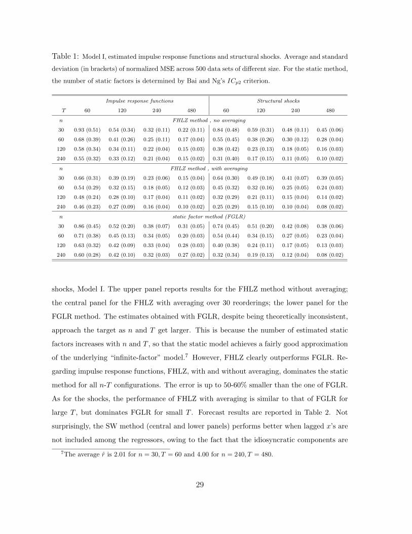
Table 1: Model I, estimated impulse response functions and structural shocks. Average and standard
deviation (in brackets) of normalized MSE across 500 data sets of different size. For the static method,
the number of static factors is determined by Bai and Ng’s ICp2 criterion.
Impulse response functions Structural shocks
T 60 120 240 480 60 120 240 480
n FHLZ method , no averaging
30 0.93 (0.51) 0.54 (0.34) 0.32 (0.11) 0.22 (0.11) 0.84 (0.48) 0.59 (0.31) 0.48 (0.11) 0.45 (0.06)
60 0.68 (0.39) 0.41 (0.26) 0.25 (0.11) 0.17 (0.04) 0.55 (0.45) 0.38 (0.26) 0.30 (0.12) 0.28 (0.04)
120 0.58 (0.34) 0.34 (0.11) 0.22 (0.04) 0.15 (0.03) 0.38 (0.42) 0.23 (0.13) 0.18 (0.05) 0.16 (0.03)
240 0.55 (0.32) 0.33 (0.12) 0.21 (0.04) 0.15 (0.02) 0.31 (0.40) 0.17 (0.15) 0.11 (0.05) 0.10 (0.02)
n FHLZ method , with averaging
30 0.66 (0.31) 0.39 (0.19) 0.23 (0.06) 0.15 (0.04) 0.64 (0.30) 0.49 (0.18) 0.41 (0.07) 0.39 (0.05)
60 0.54 (0.29) 0.32 (0.15) 0.18 (0.05) 0.12 (0.03) 0.45 (0.32) 0.32 (0.16) 0.25 (0.05) 0.24 (0.03)
120 0.48 (0.24) 0.28 (0.10) 0.17 (0.04) 0.11 (0.02) 0.32 (0.29) 0.21 (0.11) 0.15 (0.04) 0.14 (0.02)
240 0.46 (0.23) 0.27 (0.09) 0.16 (0.04) 0.10 (0.02) 0.25 (0.29) 0.15 (0.10) 0.10 (0.04) 0.08 (0.02)
n static factor method (FGLR)
30 0.86 (0.45) 0.52 (0.20) 0.38 (0.07) 0.31 (0.05) 0.74 (0.45) 0.51 (0.20) 0.42 (0.08) 0.38 (0.06)
60 0.71 (0.38) 0.45 (0.13) 0.34 (0.05) 0.20 (0.03) 0.54 (0.44) 0.34 (0.15) 0.27 (0.05) 0.23 (0.04)
120 0.63 (0.32) 0.42 (0.09) 0.33 (0.04) 0.28 (0.03) 0.40 (0.38) 0.24 (0.11) 0.17 (0.05) 0.13 (0.03)
240 0.60 (0.28) 0.42 (0.10) 0.32 (0.03) 0.27 (0.02) 0.32 (0.34) 0.19 (0.13) 0.12 (0.04) 0.08 (0.02)
shocks, Model I. The upper panel reports results for the FHLZ method without averaging;
the central panel for the FHLZ with averaging over 30 reorderings; the lower panel for the
FGLR method. The estimates obtained with FGLR, despite being theoretically inconsistent,
approach the target as n and T get larger. This is because the number of estimated static
factors increases with n and T , so that the static model achieves a fairly good approximation
of the underlying “infinite-factor” model.7 However, FHLZ clearly outperforms FGLR. Re-
garding impulse response functions, FHLZ, with and without averaging, dominates the static
method for all n-T configurations. The error is up to 50-60% smaller than the one of FGLR.
As for the shocks, the performance of FHLZ with averaging is similar to that of FGLR for
large T , but dominates FGLR for small T . Forecast results are reported in Table 2. Not
surprisingly, the SW method (central and lower panels) performs better when lagged x’s are
not included among the regressors, owing to the fact that the idiosyncratic components are
7The average r is 2.01 for n = 30, T = 60 and 4.00 for n = 240, T = 480.
29

serially uncorrelated. Indeed, we are comparing forecasts of the common components of the
x’s, i.e. the χ’s, rather than the x’s themselves. FHLZ forecasts (with averaging) outperforms
SW for all (n, T ) configurations, with an improvement ranging from 20 to 40%.8 Observe
that here we no longer impose the correct q, but estimate it with Hallin and Liska’s (2007)
criterion, so that both forecasts in the upper an central panels are feasible.
Table 2: Model I, one-step-ahead forecasts. Average and standard deviation (in brackets) of the
normalized mean square deviation from the population forecasts across 500 data sets of different size.
For the dynamic method, the number of dynamic factors is determined by Hallin and Liska’s log
criterion. For the static method, the number of static factors is determined by Bai and Ng’s ICp2
criterion.
T = 60 T = 120 T = 240 T = 480
FHLZ method, with averaging
n = 30 0.97 (0.65) 0.91 (1.06) 0.73 (0.61) 0.74 (0.67)
n = 60 0.82 (0.32) 0.68 (0.35) 0.59 (0.95) 0.50 (0.35)
n = 120 0.74 (0.21) 0.58 (0.16) 0.47 (0.27) 0.39 (0.22)
n = 240 0.70 (0.18) 0.53 (0.14) 0.41 (0.14) 0.33 (0.14)
static factor method (SW), with lagged x’s
n = 30 2.58 (3.46) 1.65 (2.99) 1.12 (1.81) 0.89 (0.88)
n = 60 2.17 (2.22) 1.28 (1.00) 0.99 (2.31) 0.73 (0.61)
n = 120 1.94 (1.53) 1.16 (0.72) 0.83 (0.90) 0.64 (0.43)
n = 240 1.87 (1.51) 1.08 (0.62) 0.75 (0.47) 0.60 (0.35)
static factor method (SW), no lagged x’s
n = 30 1.90 (2.62) 1.33 (2.05) 0.94 (0.95) 0.80 (0.74)
n = 60 1.52 (1.54) 1.02 (0.75) 0.86 (1.84) 0.68 (0.54)
n = 120 1.32 (0.89) 0.89 (0.48) 0.72 (0.66) 0.61 (0.39)
n = 240 1.24 (0.69) 0.82 (0.41) 0.64 (0.38) 0.56 (0.33)
Table 3 reports results for Model II, estimation of impulse response functions and struc-
tural shocks. Here both FHLZ and FGLR are consistent. Somewhat surprisingly, FHLZ (with
averaging, upper panel) over-performs FGLR for all (r, q) configurations. With this model,
Bai and Ng’s criterion tends to underestimate the number of factors.9 Hence, we computed
the (unfeasible) FGLR estimation obtained by imposing the correct r (lower panel), to see
8FHLZ without averaging, not reported here, performs better than SW but worse than FHLZ with
averaging, in line with the results in Table 1.9On average, r is smaller than r for all n and T configurations.
30

Table 3: Model II, estimated impulse response functions and structural shocks. Average and standard
deviation (in brackets) of the normalized MSE across 500 data sets with different configurations of
static and dynamic factors. For the static method, the number of static factors is determined by Bai
and Ng’s ICp2 criterion.
Impulse response functions Structural shocks
r 4 6 8 12 4 6 8 12
q FHLZ method, with averaging
2 0.13 (0.05) 0.11 (0.05) 0.10 (0.05) 0.09 (0.07) 0.17 (0.08) 0.12 (0.07) 0.10 (0.06) 0.08 (0.07)
4 0.15 (0.09) 0.15 (0.11) 0.14 (0.15) 0.27 (0.15) 0.22 (0.16) 0.17 (0.17)
6 0.17 (0.09) 0.15 (0.10) 0.34 (0.13) 0.24 (0.16)
FGLR method, r determined with ICp2
2 0.16 (0.14) 0.16 (0.13) 0.15 (0.13) 0.12 (0.14) 0.21 (0.25) 0.17 (0.26) 0.12 (0.19) 0.08 (0.13)
4 0.18 (0.15) 0.19 (0.16) 0.20 (0.23) 0.35 (0.26) 0.31 (0.28) 0.23 (0.28)
6 0.20 (0.13) 0.22 (0.15) 0.43 (0.22) 0.35 (0.25)
FGLR method , r assumed known
2 0.10 (0.07) 0.09 (0.07) 0.08 (0.07) 0.07 (0.06) 0.17 (0.14) 0.13 (0.13) 0.12 (0.10) 0.11 (0.06)
4 0.14 (0.12) 0.15 (0.14) 0.14 (0.19) 0.28 (0.22) 0.25 (0.23) 0.21 (0.23)
6 0.18 (0.13) 0.17 (0.14) 0.38 (0.21) 0.28 (0.21)
whether the above result can be ascribed to underestimation of r. In general, FGLR performs
better when imposing the correct number of factors; nonetheless, FHLZ still exhibits the best
performance in most cases.
Forecasts errors, reported in Table 4, confirm the result that FHLZ performs better than
SW for most (r, q) configurations.
5 Conclusions
An estimate of the common-component spectral density matrix ΣΣΣχ is obtained using the
frequency-domain principal components of the observations xit. The central idea of the
present paper is that, because ΣΣΣχ has large dimension but small rank q, a factorization of ΣΣΣχ
can be obtained piecewise. Precisely, the factorization of ΣΣΣχ only requires the factorization
of (q + 1)-dimensional subvectors of χχχt. Under our assumption of rational spectral density
for the common components, this implies that the number of parameters to estimate grows
31

as n, not n2.
The rational spectral density assumption also has the important consequences that χχχt has
a finite autoregressive representation and that the dynamic factor model can be transformed
into the static model zt = Rvt+φφφt, where zt = A(L)xt. We construct estimators for A(L), R
and vt starting with a standard non-parametric estimator of the spectral density of the x’s.
This implies a slower rate of convergence as compared to the usual T−1/2. However, in
Section 3, we prove that our estimators for A(L), R and vt do not undergo any further
reduction in their speed of convergence.
The main difference of the present paper with respect to previous literature on GDFM’s
is that although we make use of a parametric structure for the common components, we do
not make the standard, but quite restrictive assumption that our dynamic factor model has
a static representation of the form (1.4). Section 4 provides important empirical support to
the richer dynamic structure of unrestricted GDFM’s.
Table 4: Model II, one-step-ahead forecasts. Average and standard deviation (in brackets) of the
normalized mean square deviations from the population forecasts, across 500 data sets with different
configurations of static and dynamic factors. For the dynamic method, the number of dynamic factors
is determined by Hallin and Liska’s log criterion. For the static method, the number of static factors
is determined by Bai and Ng’s ICp2 criterion.
r = 4 r = 6 r = 8 r = 12
FHLZ method, with averaging
q = 2 0.79 (1.59) 0.68 (0.75) 0.59 (0.97) 0.56 (0.52)
q = 4 0.44 (0.36) 0.44 (0.28) 0.40 (0.20)
q = 6 0.40 (0.28) 0.38 (0.18)
static factor method (SW), no lagged x’s
q = 2 1.00 (2.10) 0.67 (1.04) 0.52 (64) 0.49 (0.66)
q = 4 0.61 (1.37) 0.53 (0.67) 0.43 (0.37)
q = 6 0.50 (0.58) 0.42 (0.34)
32

References
[1] Ahn, S.C., and A.R. Horenstein (2013) Eigenvalue ratio test for the number of factors,
Econometrica 81, 1203-1227.
[2] Alessi, L., M. Barigozzi and M. Capasso (2010) Improved penalization for determining
the number of factors in approximate factor models. Statistics & Probability Letters 80,
1806-1813.
[3] Amengual, D. and M. Watson, (2007) Consistent estimation of the number of dynamic
factors in a large N and T panel, Journal of Business and Economic Statistics, 25,
91-96.
[4] Anderson, B. and M. Deistler (2008a). Properties of zero-free transfer function matrices,
SICE Journal of Control, Measurement and System Integration 1, 1-9.
[5] Anderson, B. and M. Deistler (2008b). Generalized linear dynamic factor models—A
structure theory, 2008 IEEE Conference on Decision and Control.
[6] Bai, J. and S. Ng (2002). Determining the number of factors in approximate factor
models, Econometrica 70, 191-221.
[7] Bai, J. and S. Ng, (2007). Determining the number of primitive shocks in factor models,
Journal of Business and Economic Statistics, 25, 52-60.
[8] Brillinger, D. R. (1981). Time Series: Data Analysis and Theory, San Francisco: Holden-
Day.
[9] Forni, M., M. Hallin, M. Lippi and L. Reichlin (2000). The generalized dynamic factor
model: identification and estimation, The Review of Economics and Statistics 82, 540-
554.
[10] Forni, M., M. Hallin, M. Lippi and L. Reichlin (2004). The generalized dynamic factor
model : consistency and rates, Journal of Econometrics 119, 231-255.
[11] Forni, M., M. Hallin, M. Lippi and L. Reichlin (2005). The generalized factor model:
one-sided estimation and forecasting, Journal of the American Statistical Association
100, 830-40.
33

[12] Forni, M., M. Hallin, M. Lippi and P. Zaffaroni (2015). Dynamic factor models with
infinite-dimensional factor space: one-sided representations, Journal of Econometrics
185, 359-371.
[13] Forni, M., D. Giannone, M. Lippi and L. Reichlin (2009). Opening the black box: struc-
tural factor models with large cross-sections, Econometric Theory 25, 1319-1347.
[14] Forni, M. and M. Lippi (2001). The generalized dynamic factor model: representation
theory, Econometric Theory 17, 1113-1341.
[15] Franklin, J.N. (2000). Matrix Theory , New York: Dover Publications.
[16] Hallin M. and R. Liska (2007). Determining the number of factors in the general dynamic
factor model, Journal of the American Statistical Association 102, 603- 617.
[17] Hannan, E.J. (1970). Multiple Time Series, New York: Wiley.
[18] Lancaster, P. and M. Tismenetsky (1985). The Theory of Matrices, second edition, New
York: Academic Press.
[19] Liu, W.D. and W.B. Wu (2010). Asymptotics of spectral density estimates, Econometric
Theory, 26 , 1218-1245.
[20] Onatski, A. (2009). Testing hypotheses about the number of factors in large factor
models, Econometrica 77, 1447-1479.
[21] Onatski, A. (2010) Determining the number of factors from empirical distribution of
eigenvalues, The Review of Economics and Statistics 92, 1004-1016.
[22] Shao, W. and W.B. Wu (2007). Asymptotic spectral theory for nonlinear time series,
Annals of Statistics 35, 1773-1801.
[23] Stock, J.H. and M.W. Watson (2002a). Macroeconomic Forecasting Using Diffusion
Indexes, Journal of Business and Economic Statistics 20, 147-162.
[24] Stock, J.H. and M.W. Watson (2002b). Forecasting using principal components from a
large number of predictors, Journal of the American Statistical Association 97, 1167-
1179.
34

[25] Wu, W.B. (2005). Nonlinear system theory: Another look at dependence. Proceedings
of the National Academy of Sciences USA, 102, 14150-14154.
[26] Wu, W.B. and P. Zaffaroni (2015). On Uniform Moments Convergence of Spectral Den-
sity Estimates, arXiv 1505.03659, available at http://arxiv.org/abs/1505.03659.
35

Appendix
A Proof of Proposition 6
Adding and subtracting E(σxij(θ∗h)) within the absolute value in E
(max|h|≤BT
∣∣σxij(θ∗h)− σxij(θ∗h)∣∣2 )
and re-arranging gives
E(
max|h|≤BT
∣∣σxij(θ∗h)− σxij(θ∗h)∣∣2 ) ≤ E( max
|h|≤BT
∣∣σxij(θ∗h)− Eσxij(θ∗h)∣∣2 )+
(max|h|≤BT
∣∣Eσxij(θ∗h)− σxij(θ∗h)∣∣2 ).
The first term (variance) on the right hand side of the above inequality satisfies
E(
max|h|≤BT
∣∣σxij(θ∗h)− Eσxij(θ∗h)∣∣2 ) ≤ C∗(BT logBT /T ),
where C∗ depends only on p (see Assumption 8), ρ1 (see Proposition 5), δ (see Assumption 9).
This is proved in Wu and Zaffaroni (2015) Lemma 10, with ν = 2.
As for the second term (the squared bias), simple calculations give
Sij(θ) = 2π(Eσxij(θ)− σxij(θ)
)=
T−1∑l=−T+1
(1− |l|
T
)K
(l
BT
)γxij,l e
−ılθ −∞∑
l=−∞γxij,l e
−ılθ
≤
∣∣∣∣∣T−1∑
l=−T+1
(K
(l
BT
)− 1
)γxij,l e
−ılθ
∣∣∣∣∣+
∣∣∣∣∣T−1∑
l=−T+1
K
(l
BT
)|l|Tγxij,l e
−ılθ
∣∣∣∣∣+
∣∣∣∣∣∣∑|l|≥T
γxij,l e−ılθ
∣∣∣∣∣∣= ATij(θ) + BTij(θ) + CTij(θ).
Assumptions 2 and 4 imply that, for some φ ∈ (0, 1) and someD, |γxij,l| ≤ |γχij,l|+|γ
ξij,l| ≤ Dφ
|l|,
for all i and j (see equation 2.8)). This inequality and Assumption 9(i) ensure that, for some F
and all i, j and θ, ATij(θ) ≤ FD∑∞
l=−∞ φ|l|(|l|/BT )κ ≤ [2DFφ/(1 − φ)2]T−δκ = HT−δκ.
Moreover, BTij(θ) ≤ DT−1∑∞
l=−∞ φ|l||l| = [2Dφ/(1 − φ)2]T−1 = KT−1, for all i, j, and θ.
Finally, CTij(θ) ≤ D∑|l|≥T φ
|l||l|κ/T κ, since |l|κ/T κ ≥ 1 for |l| ≥ T . Hence, it follows that
CTij(θ) ≤MT−κ ≤MT−δκ for all i, j and θ. Thus Sij(θ)/2π ≤ KT−1+(H+M)T−δκ ≤ PT−µ,
where µ = min(δκ, 1), for all i, j and θ. Now, 2δκ > 1 − δ > 1 − δ, by Assumption 9(ii).
Hence, max|h|≤BT
∣∣∣Eσxij(θ∗h)− σxij(θ∗h)∣∣∣2 ≤ P 2T−2µ ≤ C∗∗(BT logBT /T ) for all i and j. �
B Proof of Proposition 7
The proof below closely follows Forni et al. (2009). Denote by µj(A), j = 1, 2, . . . , s, the (real)
eigenvalues, in decreasing order, of an s × s Hermitian matrix A, and by ‖B‖ =√µ1(BB)
36

the spectral norm of an s1× s2 matrix B. The norm ‖B‖ coincides with the Euclidean norm
of B when B is a column matrix and is equal to |µ1(B)| when B is square and Hermitian.
Recall that, if B1 is s1 × s2 and B2 is s2 × s3, then
‖B1B2‖ ≤ ‖B1‖‖B2‖. (B.1)
We will use the fact that, for any two s× s Hermitian matrices A1 and A2,
|µj(A1 + A2)− µj(A1)| ≤ ‖A2‖, j = 1, . . . , s. (B.2)
This fact is an obvious consequence of Weyl’s inequality µj(A1 + A2) ≤ µj(A1) + µ1(A2)
(Franklin, 2000, p. 157, Theorem 1).
The proof of Proposition 7 is divided into several intermediate propositions. Denote by Si
the n × 1 matrix with 1 in entries (i, 1) and 0 elsewhere, so that S ′1A is the i-th row of A,
and define ρT = T/BT logBT .
As most of the arguments below depend on equalities and inequalities that hold for
all θ ∈ [−π, π], the notation has been simplified by dropping θ. Properties holding for
max|h|≤BTF (θh), where F is some function of θ, are often phrased as holding for F uniformly
in θ. The meaning of uniformity in i, or i and j, has been clarified in the statement of
Proposition 7.
All lemmas in this Appendix hold and are proved under Assumptions 1 through 10.
Lemma 1 As T → ∞ and n→∞,
(i) max|h|≤BTn−1‖ΣΣΣx −ΣΣΣx‖ = OP (ρ
−1/2T );
(ii) max|h|≤BTn−1/2‖S ′i(ΣΣΣx −ΣΣΣx)‖ = OP (ρ
−1/2T ) uniformly in i;
(iii) max|h|≤BTn−1‖ΣΣΣx −ΣΣΣχ‖ = OP (max(n−1, ρ
−1/2T ));
(iv) max|h|≤BTn−1/2‖S ′i(ΣΣΣx −ΣΣΣχ)‖ = OP (max(n−1/2, ρ
−1/2T )) = OP (ζnT ) uniformly in i.
Proof. We have
µ1((ΣΣΣx −ΣΣΣx)(˜Σ˜ΣΣx − ΣΣΣx)) ≤ trace((ΣΣΣx −ΣΣΣx)(
˜Σ˜ΣΣx − ΣΣΣx)) =
n∑i=1
n∑j=1
|σxij − σxij |2.
Using (3.4) and the Markov inquality,
n−2 max|h|≤BT
n∑i=1
n∑j=1
|σxij − σxij |2 ≤ n−2n∑i=1
n∑j=1
max|h|≤BT
|σxij − σxij |2 ≤ Cρ−1T .
37

Statement (i) follows. In the same way,
n−1S ′i(ΣΣΣx −ΣΣΣx)(˜Σ˜ΣΣx − ΣΣΣx)Si = n−1
n∑j=1
|σxij − σxij |2 ≤ Cρ−1T ,
where C is independent of i. Statement (ii) follows. As regards (iii), ΣΣΣx = ΣΣΣχ + ΣΣΣξ implies
that ΣΣΣx −ΣΣΣχ = ΣΣΣx −ΣΣΣx + ΣΣΣξ, so that, by the triangle inequality for matrix norm,
‖ΣΣΣx −ΣΣΣχ‖ ≤ ‖ΣΣΣx −ΣΣΣx‖+ ‖ΣΣΣξ‖.
The statement follows from (i) and the fact that ‖ΣΣΣξ‖ = λξ1 is bounded. Statement (iv) is
obtained in a similar way, using (ii) instead of (i). �
Lemma 2 As T → ∞ and n→∞,
(i) max|h|≤BTn−1
∣∣∣λxf − λχf ∣∣∣ = OP (max(n−1, ρ−1/2T )) for f = 1, 2, . . . , q;
(ii) letting
Gχ =
Iq if λχq = 0,
n(ΛΛΛχ)−1 otherwise,and Gx =
Iq if λxq = 0,
n(ΛΛΛx)−1 otherwise,,
max|h|≤BTn−1‖ΛΛΛχ‖ and max|h|≤BT
‖Gχ‖ are O(1), max|h|≤BTn−1‖ΛΛΛx‖ and max|h|≤BT
‖Gx‖
are OP (1).
Proof. Setting A1 = ΣΣΣχ and A2 = ΣΣΣx −ΣΣΣχ, (B.2) yields |λxf − λχf | ≤ ‖ΣΣΣ
x −ΣΣΣχ‖; hence,
statement (i) follows from Lemma 1 (iii). Boundedness of n−1‖ΛΛΛχ‖ and ‖Gχ‖, uniformly
in θ, is a consequence of Assumption 3. Boundedness in probability of n−1‖ΛΛΛx‖ and ‖Gx‖,
uniformly in θ, follows from statement (i). �
Lemma 3 As T → ∞ and n→∞,
(i) max|h|≤BTn−1‖PχPxΛΛΛx −ΛΛΛχPχPx‖ = OP (max(n−1, ρ
−1/2T ));
(ii) max|h|≤BT‖ ˜PxPχPχPx − Iq‖ = OP (max(n−1, ρ
−1/2T ));
(iii) there exist diagonal complex orthogonal matrices Wq = diag(w1 w2 · · · wq), |wj |2 = 1,
j = 1, . . . , q depending on n and T , such that max|h|≤BT‖ ˜PxPχ−Wq‖ = OP (max(n−1, ρ
−1/2T )).
Proof. Using inequality (B.1) and the fact that ‖Pχ‖ = ‖Px‖ = 1, we have
‖PχPxΛΛΛx −ΛΛΛχPχPx‖ = ‖Pχ(ΣΣΣx −ΣΣΣχ)Px‖ ≤ ‖ΣΣΣx −ΣΣΣχ‖.
Statement (i) thus follows from Lemma 1 (iii). Turning to (ii), set
38

a = ˜PxPχPχPx, b =[˜PxPχPχPx
]n−1ΛΛΛxGx = ˜PxPχ
[PχPxn−1ΛΛΛx
]Gx,
c = ˜PxPχ[n−1ΛΛΛχPχPx
]Gx=
[n−1 ˜PxΣΣΣχPx
]Gx, d =
[n−1 ˜PxΣΣΣxPx
]Gx = n−1ΛΛΛxGx,
and f = Iq: we have∥∥∥ ˜PxPχPχPx − Iq
∥∥∥ ≤ ‖a− b‖+ ‖b− c‖+ ‖c− d‖+ ‖d− f‖. (B.3)
Using Lemma 2, statement (i), and the boundedness in probability, uniformly in θ, of ‖ ˜PxPχ‖,
‖Gx‖ and ‖ ˜PxPχPχPx‖, all terms on the right-hand side of inequality (B.3) can be shown
to be OP (max(n−1, ρ−1/2T )), uniformly in θ.
Turning to (iii), note that, from statement (i), n−1 ˜PxhPχ
k (λχk−λxh) = OP (max(n−1, ρT
−1/2)).
Assumption 3 (asymptotic separation of the eigenvalues λχf (θ)) implies that, for h 6= k,
˜PxhPχ
k = OP (max(n−1, ρT−1/2)). Moreover,
∑qf=1 |
˜PxhPχ
f |2 − 1 = OP (max(n−1, ρT
−1/2))
from statement (ii). Therefore,
| ˜PxhPχ
h|2 − 1 = (| ˜Px
hPχh| − 1)(|Pχ
hPxh|+ 1) = OP (max(n−1, ρT
−1/2)).
The conclusion follows. �
Note that Lemma 3 clearly also holds for n−1‖ ˜PxPχΛΛΛχ− ΛΛΛx ˜PxPχ‖, ‖PχPx ˜PxPχ − Iq‖
and ‖ ˜PχPx − ˜Wq‖.
Lemma 4 As T → ∞ and n→∞,
max|h|≤BT
‖S ′i(Pχ(ΛΛΛχ)1/2Wq − Px(ΛΛΛx)1/2
)‖ = OP (ζnT ), (B.4)
uniformly in i.
Proof. We have
‖S ′i(Pχ(ΛΛΛχ)1/2Wq − Px(ΛΛΛx)1/2)‖ ≤ ‖S ′i(n1/2PχWq − n1/2Px)(n−1ΛΛΛχ)1/2‖
+‖S ′iPx(n−1/2(ΛΛΛχ)1/2 − n−1/2(ΛΛΛx)1/2)‖.
By Lemma 2 (i), thus, we only need to prove that
‖n1/2S ′iPχWq − n1/2S ′iPx‖ = OP (max(n−1/2, ρT−1/2)).
Firstly, we show that
39

‖n1/2S ′iPχ‖ ≤ A, (B.5)
for some A and all θ and i. Assumption 2 implies that σχii =∑q
f=1 λχf |p
χif |
2 ≤ B, for some B
and all θ and i. As all the terms in the sum are positive, λχf |pχif |
2 = (λχf /n)n|pχif |2 ≤ B, for
all θ and i. By Assumption 3, λχf /n ≥ C > 0 for all θ and f , so that n|pχif |2 ≤ D for all θ
and i. Hence, n S ′iPχPχSi is bounded uniformly in θ and i; (B.5) follows. Next, define
g = n1/2S ′iPχ[Wq
], h = n1/2S ′iPχ
[PχPx
]= n1/2S ′iPχ[PχPxΛx/n](Λx/n)−1,
i = n1/2S ′iPχ[(Λχ/n)PχPx](Λx/n)−1 = [n−1/2S ′iΣΣΣχ]Px(Λx/n)−1,
andj = [n−1/2S ′iΣΣΣx]Px(Λx/n)−1 = n1/2S ′iPx.
Lemma 3(iii) and inequality (B.5) imply that ‖g−h‖ is OP (max(n−1, ρT−1/2)) uniformly in θ
and i. Inequality (B.5), Lemma 3(i) and Lemma 2(ii) imply that ‖h−i‖ isOP (max(n−1, ρT−1/2))
uniformly in θ and i. Moreover, ‖Px(Λx/n)−1‖ = OP (1), uniformly in θ, by Lemma 2(ii)
and the fact that ||Px|| = 1. Thus, using Lemma 1(iv), it is seen that, uniformly in θ and i,
‖i− j‖ is OP (max(n−1/2, ρT−1/2)). The result follows. �
Proposition 7 now follows from
ΣΣΣχ =
[Px(ΛΛΛx)1/2
] [(ΛΛΛx)1/2 ˜Px
]= PχΛΛΛχ ˆP
χ.
and
ΣΣΣχ =[Px (ΛΛΛx)1/2 Wq
] [ˆWq (ΛΛΛx)1/2 Px
]= PχΛΛΛχPχ.
�
Note that the eigenvectors Pχ are defined up to post-multiplication by a complex diagonal
matrix with unit modulus diagonal entries. In particular, using the eigenvectors ΠΠΠχ = PχWq,
(B.4) would hold for ΠΠΠχ(ΛΛΛχ)1/2− Px(ΛΛΛx)1/2 . For the sake of simplicity, we avoid introducing
a new symbol and henceforth refer to the result of Lemma 4 as
max|h|≤BT
‖S ′1(Pχ(ΛΛΛχ)1/2 − Px(ΛΛΛx)1/2)‖ = OP (max(n−1/2, ρT−1/2)) (B.6)
and the result of Lemma 3(iii) as
‖ ˜PxPχ − Iq‖ = OP (max(n−1, ρT−1/2)).
In the same way, we drop Wq in Lemmas 6, 7, 8, though not in the conclusion of Appendix D,
nor in Appendix E.
40

C Proof of Proposition 9
To start with, note that, as the extreme right-hand side in (3.6) contains the term
πB
BT
∑|h|≤BT
(|eı`θ∗h−1 − eı`θ∗h−1 |+ |eı`θ∗h−1 − eı`θ∗h−1 |
),
convergence in (3.7) is not uniform with respect to `. However, estimation of the matrices Bχk
and Cχjk only requires the covariances γχij,` with ` ≤ S, where S is finite. Therefore, Propo-
sition 8 implies that ‖Bχk −Bχ
k‖ and ‖Cχjk −Cχ
jk‖ are OP (max(n−1/2, ρ−1/2T )). From (2.16),
applying (B.1),
‖A[k] −A[k]‖ ≤ ‖Bχk‖‖(C
χkk)−1 −
(Cχkk
)−1 ‖+ ‖Bχk −Bχ
k‖‖(Cχkk
)−1 ‖.
By Assumption 2, ‖Bχk‖ ≤ W for some constant W > 0, so that ‖Bχ
k‖ is bounded in
probability. By Assumptions 2 and 7, ‖(Cχkk
)−1 ‖ ≤ W1 for some W1 > 0. Observing that
the entries of(Cχkk
)−1are rational functions of the entries of Cχ
kk, and that det(Cχkk
)> 0 by
Assumption 7, Proposition 8 implies that ‖(Cχkk)−1 −
(Cχkk
)−1 ‖ is OP (max(n−1/2, ρ−1/2T )).
The conclusion follows. �
D Proof of Proposition 10
Consider the static model Znt = Rvt + ΦΦΦnt. If Znt = A(L)xnt were observed, i.e. if the
matrices A(L) were known, then Proposition 10, with an estimator of R based on the em-
pirical covariance ΓΓΓz of the Znt, would be straightforward. However, we only have access
to Znt = A(L)xt and its empirical covariance matrix ΓΓΓz, which makes the estimation of R
significantly more difficult. The consistency properties of our estimator follow from the con-
vergence result (D.4) in Lemma 11, which establishes the asymptotic behavior of the diffe-
rence ΓΓΓz − ΓΓΓz; Lemmas 5 through 10 are but a preparation for that key result. All lemmas
in this Appendix hold, and are proved under Assumptions 1 through 10.
Lemma 5 For f = 1, . . . , q, as T → ∞ and n→∞,
(i) | pχif |= O(n−1/2) and | pxif |= OP (n−1/2), uniformly in θ and i;
(ii) for any positive integer d, n−1∑n
i=1 | pχif |
d and n−1∑n
i=1 | pxif |d are O(n−d/2)
and OP (n−d/2), respectively, uniformly in θ.
41

Proof. The first part of (i) follows from B.5. As regards the second part, let us first prove
that σxii is OP (1) uniformly in θ and i. We have
maxh
σxii(θh) ≤ maxh
σxii(θh) + maxh|σxii(θh)− σxii(θh)|.
By Assumptions 2 and 4, the first term on the right-hand side is bounded uniformly in i. By
the Markov inequality and (3.4),
P (maxh|σxii(θh)− σxii(θh)| ≥ η) ≤ η−2E
(max|h|≤BT
|σxii(θ∗h)− σxii(θ∗h)|2)
≤ η−2C(T−1BT logBT )
Thus, for any ε > 0, we can set
η(ε) ≥[
maxT C(T−1BT logBT )
ε
]1/2
,
irrespective of θh and i. Because σχii ≤ σxii, we have that σχii =∑q
f=1 λxf |pxif |2 = OP (1)
uniformly in θ and i. As all the terms in the sum are positive, λxf |pxif |2 = (λxf/n)n|pxif |2
is OP (1) as well, uniformly in θ and i. Lemma 2 (i) and Assumption 3 imply that λxf/n
is OP (1) and bounded away from zero in probability uniformly in θ. The conclusion follows.
Statement (ii) is proved by induction. Consider Pχf . It follows from statement (i)
that n−1∑n
i=1 |pχif | is O
(n−1/2
), uniformly in θ. Assume now that the result holds for d− 1,
with d ≥ 2. Using the first part of (i), uniformity in i in particular, we have
n−1n∑i=1
| pχif |d = n−1
n∑i=1
| pχif |d−1| pχif |
≤(maxi≤n|pχif |
)n−1
n∑i=1
| pχif |d−1= O(n−1/2 n−(d−1)/2) = O
(n−d/2
).
The same argument applies to Pxf . �
Lemma 6 As T → ∞ and n→∞,
max|h|≤BT
∥∥∥Pχ(ΛΛΛχ)1/2 − Px
(ΛΛΛx)1/2∥∥∥ = OP (n1/2 max(n−1, ρ
−1/2T )). (D.1)
Proof. The left-hand side of (D.1) equals the left-hand side of (B.4) when Si is replaced
by In. The proof goes along the same lines as that of Lemma 4. Firstly, ‖n1/2Pχ‖ is O(n1/2).
42

Both ‖g−h‖ and ‖h− i‖ are OP (n1/2 max(n−1, ρ−1/2T )). As for ‖i− j‖, the conclusion follows
from Lemma 1 (iii). �
Lemma 7 For f = 1, . . . , q, as T → ∞ and n→∞, |pχif−pxif | = OP (n−1/2 max(n−1/2, ρ
−1/2T )),
uniformly in θ and i.
Proof. By (B.6), pχif (λχf )1/2 − pxif (λxf )1/2 = OP (max(n−1/2, ρ−1/2T )), uniformly in θ and i.
Now,
pχif (λχf )1/2 − px(λxf )1/2 = pχif
((λχf )1/2 − (λxf )1/2
)+ (λxf )1/2
(pχif − p
xif
). (D.2)
The former term on the right-hand side can be written as
n1/2pχif(λχf − λ
xf )/n(
(λχf )1/2 + (λxf )1/2)/n1/2
,
which isOP (max(n−1, ρ−1/2T )), uniformly in θ and i, since the numerator isOP (max(n−1, ρ
−1/2T )),
uniformly in θ, by Lemma 2(i); the denominator is bounded away from zero, uniformly in θ,
by Assumption 3 and n1/2pχif is O(1), uniformly in θ and i, by Lemma 5(i). It follows that
the latter term in (D.2), (λxf )1/2(pχif − p
xif
), is OP (max(n−1/2, ρ
1/2T )), uniformly in θ and i.
By Lemma 2(ii), n−1/2(λxf )1/2 is bounded away from zero in probability, uniformly in θ. The
result follows. �
Lemma 8 For any integer d ∈ N, for f = 1, . . . , q, as T → ∞ and n→∞,
n−1n∑i=1
| pχif − pxif |d= OP ((n−1 max(n−1, ρ−1
T ))d/2), (D.3)
uniformly in θ.
Proof. Lemma 7 implies that(maxi≤n | pχif−p
xif |), and therefore n−1
∑ni=1 | pxif − p
χif |,
are OP ((n−1 max(n−1, ρ−1T ))1/2), uniformly in θ. By induction, assume now that the result
holds for d− 1, d ≥ 2. We have
n−1∑n
i=1 | pχif − p
xif |d = n−1
∑ni=1 | p
χif − p
xif |d−1| pχif − p
xif |
≤(maxi≤n | pχif−p
xif |)n−1
∑ni=1 | p
χif−p
xif |d−1
= OP ((n−1 max(n−1, ρ−1T ))1/2) OP
((n−1 max(n−1, ρ−1
T ))(d−1)/2),
uniformly in θ, as was to be shown. �
43

Lemma 9 For n→∞ and T →∞, uniformly in θ,
(i) n−2n∑i=1
n∑j=1
| σχij(θ)− σχij(θ)|
d = OP ((max(n−1, ρ−1T ))d/2);
(ii) n−1n∑i=1
| σχij(θ)− σχij(θ) |
d= OP ((max(n−1, ρ−1T ))d/2) for any 1 ≤ j ≤ n;
(iii) n−1n∑i=1
| σχii(θ)− σχii(θ) |
d= OP ((max(n−1, ρ−1T ))d/2).
Proof. We have
σχij − σχij = (λx1 − λ
χ1 )pxi1
¯pxj1 + · · ·+ (λxq − λχq )pxiq¯pxjq + λχ1 p
xi1(¯pxj1 − p
χj1)
+λχ1 pχj1(pxi1 − p
χi1) + . . .+ λχq p
xiq(
¯pxjq − pχjq) + λχq p
χjq(p
xiq − p
χiq).
Using the triangular and Cr inequalities, by Lemmas 2, 5 and 8,
n−2n∑i=1
n∑j=1
| σχij − σχij |
d
≤ (3q)d−1(| λχ1 − λ
x1 |d
(n−1
n∑i=1
| pxi1 |d)2
+ · · ·+ | λχq − λxq |d(n−1
n∑i=1
| pxiq |d)2)
+ (3q)d−1(λχ1 )d(n−2
n∑i=1
| pxi1 |dn∑j=1
| pχj1 − pxj1 |d +n−2
n∑j=1
| pχj1 |d
n∑i=1
| pχi1 − pxi1 |d
)+ · · ·
+ (3q)d−1(λχq )d(n−2
n∑i=1
| pxiq |dn∑j=1
| pχjq − pxjq |d +n−2
n∑j=1
| pχjq |d
n∑i=1
| pχiq − pxiq |d
)= OP ((max(n−1, ρ
−1/2T ))d) +OP ((max(n−1, ρ−1
T ))d/2) = OP ((max(n−1, ρ−1T ))d/2).
Statement (i) follows. For statement (ii),
n−1n∑i=1
| σχij − σχij |
d
≤ (3q)d−1(| λχ1 − λ
x1 |d|pxj1|d n−1
n∑i=1
|pxi1|d + · · ·+ | λχq − λxq |d |pxjq|d n−1n∑i=1
| pxiq |d)
+ (3q)d−1(λχ1 )d( ∣∣∣pχj1 − pxj1∣∣∣d n−1
n∑i=1
|pxi1|d +
∣∣∣pχj1∣∣∣d n−1n∑i=1
| pχi1 − pxi1 |d
)+ · · ·
+ (3q)d−1(λχq )d(∣∣∣pχjq − pxjq∣∣∣d n−1
n∑i=1
∣∣pxiq∣∣d +∣∣∣pχjq∣∣∣d n−1
n∑i=1
| pχiq − pxiq |d
)= OP ((max(n−1, ρ
−1/2T ))d) +OP ((max(n−1, ρ−1
T ))d/2) = OP ((max(n−1, ρ−1T ))d/2).
Statement (iii) follows along the same lines, by setting j = i. �
44

Lemma 10 For n → ∞ and T → ∞, n−2S∑`=0
n∑i=1
n∑j=1
| γχij,` − γχij,`|
d and, for any given j
in {1, . . . , n}, n−1S∑`=0
n∑i=1
| γχij,` − γχij,` |
d, are OP((max(n−1, ρ−1
T ))d/2).
Proof. We have |γχij,` − γχij,`| ≤ Uij + V` +Wij , where Uij , V` and Wij are the terms in the
extreme right-hand side of (3.6). Using the Cr inequality, we get
n−2n∑i=1
n∑j=1
|γχij,0 − γχij,0|
d ≤ n−23d−1n∑i=1
n∑j=1
Udij + n−23d−1n∑i=1
n∑j=1
Vd` + n−23d−1n∑i=1
n∑j=1
Wdij .
The first term on the right-hand side is bounded in view of Lemma 9. Since ` takes only a
finite number of values, the second term is O(B−dT ) (see the proof of Proposition 9). Because
the functions σxij are of bounded variation uniformly in i and j, see Proposition 2, the third
term is O(B−dT ). The same argument used to obtain Proposition 8 applies. The second
statement is proved in the same way. �
We are now able to state and prove the main lemma of this section. Assume, without
loss of generality, that n increases by blocks of size q + 1, so that n = m(q + 1).
Lemma 11 Denoting by Z the T ×n matrix with Zit in entry (t, i), let ΓΓΓz = Z′Z/T. Then,
as n→∞ and T →∞,
n−1‖ΓΓΓz −ΓΓΓz‖ = OP (ζnT ) and n−1/2‖S ′i(ΓΓΓz −ΓΓΓz)‖ = OP (ζnT ), (D.4)
where Γz is the population covariance matrix of Znt.
Proof. Denote by Γz = Z′Z/T the empirical covariance matrix we would compute from
the Znt’s, were the matrices A(L) known. We have
‖ΓΓΓz −ΓΓΓz‖ ≤ ‖ΓΓΓz − ΓΓΓz‖+ ‖ΓΓΓz −ΓΓΓz‖, (D.5)
so that the lemma can be proved by showing that (D.4) holds with ‖ΓΓΓz − ΓΓΓz‖ replaced by
any of the two terms on the right-hand side of (D.5).
First consider ‖ΓΓΓz −ΓΓΓz‖. Since A(L) = In −A1L− · · · −ASLS , where
As =
A1s 0 · · · 0
0 A2s · · · 0
.... . .
0 0 · · · Ams
, s = 1, . . . , S
45

and A0 = In, we obtain
‖ΓΓΓz−ΓΓΓz‖2≤S∑s=0
S∑r=0
‖AsΓΓΓxs−rA
′r−AsΓΓΓ
xs−rA
′r‖2 =
S∑s=0
S∑r=0
‖As
(ΓΓΓxs−r−ΓΓΓxs−r
)A′r‖2, (D.6)
which is a sum of (S + 1)2 terms, where we set ΓΓΓxs−r = T−1∑T
t=1 xt−rx′t−s. Inspection of
the right-hand side of (D.6) shows that (D.4) holds, with ‖ΓΓΓz −ΓΓΓz‖ replaced with ‖ΓΓΓz −ΓΓΓz‖,
under Assumptions 2 and 7, and in view of Propositions 2 and 6.
Turning to ‖ΓΓΓz − ΓΓΓz‖, since
‖ΓΓΓz − ΓΓΓz‖2 ≤S∑s=0
S∑r=0
‖AsΓΓΓxs−rA
′r −AsΓΓΓ
xs−rA
′r‖2,
it is sufficient to prove that (D.4) still holds with ‖ΓΓΓz − ΓΓΓz‖ replaced with any of the
‖AsΓΓΓxs−rA
′r − AsΓΓΓ
xs−rA
′r‖’s. Denoting by ajsα, 1 ≤ α ≤ q + 1, the α-th column of Aj
s′,
we have
‖AsΓΓΓxs−rAr′ −AsΓΓΓxs−rA
r ′‖2 ≤m∑j=1
m∑k=1
q+1∑α=1
q+1∑β=1
(aj′sαΓΓΓxjk,s−ra
krβ − aj′sαΓΓΓxjk,s−ra
krβ
)2
≤ 2m∑j=1
m∑k=1
q+1∑α=1
q+1∑β=1
((ajsα − aj′sα)ΓΓΓxjk,s−ra
krβ
)2
+ 2
m∑j=1
m∑k=1
q+1∑α=1
q+1∑β=1
(aj′sαΓxjk,s−r(a
krβ − akrβ)
)2,
(D.7)
where ΓΓΓxjk,s−r is the (j, k)-block of ΓΓΓxs−r, and the second inequality follows from applying
the Cr inequality to each term of the form
(aj′sαΓΓΓxjk,s−rakrβ − aj′sαΓΓΓxjk,s−ra
krβ)2 = ((ajsα − ajsα)′ΓΓΓxjk,s−ra
krβ − aj′sαΓΓΓxjk,s−r(a
krβ − akrβ))2.
The two terms on the right-hand side of (D.7) can be dealt with in the same way. Let us
focus on the first of them. Using twice the Cauchy-Schwartz inequality, then subsequently
the Cr and Jensen inequalities, we obtain
m∑j=1
m∑k=1
q+1∑α=1
q+1∑β=1
((ajsα − ajsα)′ΓΓΓxjk,s−rakrβ)2
≤m∑j=1
m∑k=1
q+1∑α=1
q+1∑β=1
((ajsα − ajsα)′(ajsα − ajsα)ak′rβΓΓΓx′jk,s−rΓΓΓ
xjk,s−ra
krβ
=m∑k=1
q+1∑β=1
m∑j=1
q+1∑α=1
(ajsα − ajsα)′(ajsα − ajsα)ak′rβΓΓΓx′jk,s−rΓΓΓxjk,s−ra
krβ
46

≤m∑k=1
q+1∑β=1
[ m∑j=1
[ q+1∑α=1
(ajsα − ajsα)′(ajsα − ajsα)]2]1/2[ m∑
j=1
(akrβ′ΓΓΓxjk,s−r
′ΓΓΓxjk,s−rakrβ
)2]1/2= m
[ m∑j=1
[ q+1∑α=1
(ajsα − aj′sα)(ajsα − ajsα)]2]1/2 1
m
m∑k=1
q+1∑β=1
[ m∑j=1
(ak′rβΓΓΓx′jk,s−rΓΓΓ
xjk,s−ra
krβ
)2]1/2≤ AB, say,
where
A = m(q + 1)1/2[ m∑j=1
q+1∑α=1
((ajsα − ajsα)′(ajsα − ajsα)
)2]1/2and
B =1
m
m∑k=1
q+1∑β=1
[ m∑j=1
(ak′rβΓΓΓx′jk,s−rΓΓΓ
xjk,s−ra
krβ
)2 ]1/2≤
[(q + 1)/m
m∑k=1
q+1∑β=1
m∑j=1
(ak′rβΓΓΓ
x′jk,s−rΓΓΓ
xjk,s−ra
krβ
)2 ]1/2= C, say.
First consider A. Letting aj′sα = (ajsα,1 ajsα,2 · · · ajsα,q+1), note that ajsα,δ = e′αA[j]gsδ,
where eα and gsδ stand for the α-th and (s − 1)(q + 1) + δ-th unit vectors in the (q + 1)-
and (q+1)S-dimensional canonical bases, respectively. Writing, for the sake of simplicity, Bj
and Cj instead of Bχj and Cχ
jj , as defined in (2.14) and (2.15), we obtain, from (B.1), and
applying subsequently the Cr, the triangular, the Cr again and then twice the Cauchy-
Schwartz inequalities,[m∑j=1
q+1∑α=1
((ajsα − ajsα)′(ajsα − ajsα)
)2 ]1/2
≤ (q + 1)1/2( m∑j=1
q+1∑α=1
q+1∑δ=1
(ajsα,δ − ajsα,δ)
4)1/2
= (q + 1)1/2( m∑j=1
q+1∑α=1
q+1∑δ=1
[eα
((Bj −Bj)C
−1j + BjC
−1j (Cj −Cj)C
−1j
)gsδ
]4 )1/2≤ 23/2(q + 1)3/2
( m∑j=1
‖(Bj −Bj)C−1j ‖
4 + ‖BjC−1j (Cj −Cj)C
−1j ‖
4)1/2
≤ 23/2(q + 1)3/2([ m∑
j=1
‖Bj −Bj‖8]1/2[ m∑
j=1
‖C−1j ‖
8]1/2
+[ m∑j=1
‖Cj −Cj‖8]1/2[ m∑
j=1
‖BjC−1j ‖
8‖C−1j ‖
8]1/2)1/2
47

≤ 23/2(q + 1)3/2([ m∑
j=1
‖Bj −Bj‖8]1/2[ m∑
j=1
‖C−1j ‖
8]1/2
+[ m∑j=1
‖Cj −Cj‖8]1/2[ m∑
j=1
‖Bj‖16] 14[ m∑j=1
‖C−1j ‖
16‖C−1j ‖
16] 14)1/2
.
Denoting by bjiδ the entries of Bj , i = 1, . . . , q + 1, δ = 1, . . . , S(q + 1), the Cr inequality and
Lemma 10 entailm∑j=1
‖Bj −Bj‖8 ≤m∑j=1
( q+1∑i=1
S(q+1)∑δ=1
(bjiδ − bjiδ)
2)4
≤ (q + 1)6S3m∑j=1
q+1∑i=1
S(q+1)∑δ=1
(bjiδ − bjiδ)
8 = OP (m(max(n−1, ρ−1T ))4).
In a similar way, one can prove that∑m
j=1 ‖Cj −Cj‖8 is OP (m(max(n−1, ρ−1T ))4). Moreover,
Assumptions 2 and 7 together with Lemma 10 imply that∑m
j=1 ‖Bj‖16 and∑m
j=1 ‖C−1j ‖16,
as well as∑m
j=1 ‖C−1j ‖8 and
∑mj=1 ‖C
−1j ‖16, are OP (m).
Collecting terms yields
A = m(q + 1)1/2[ m∑j=1
q+1∑α=1
((ajsα − ajsα)′(ajsα − ajsα)
)2]1/2≤ 23/2(q + 1)2m
( m∑i=1
‖Ais −Ai
s‖4)1/2
= OP(m3/2 max(n−1, ρ−1
T )). (D.8)
Turning to C, we obtain, by means of similar methods,
C ≤ ((q + 1)/m)1/2{[ m∑
k=1
( q+1∑β=1
(ak′rβakrβ)2
)2]1/2[ m∑j=1
( m∑k=1
(trace[ΓΓΓx′jk,s−rΓΓΓ
xjk,s−r]
)4)1/2]}1/2
≤ ((q + 1)/m)1/2{[
(q + 1)m∑k=1
q+1∑β=1
(ak′rβakrβ)4
]1/2[ m∑j=1
( m∑k=1
(trace[ΓΓΓx′jk,s−rΓΓΓ
xjk,s−r]
)4)1/2]}1/2
≤ (q + 1)1/2[(q + 1)4
m∑k=1
q+1∑α=1
q+1∑β=1
(akr,αβ)8]1/4[
m−1m∑j=1
m∑k=1
(trace[ΓΓΓx′jk,s−rΓΓΓ
xjk,s−r]
)4]1/4≤ (q + 1)3/2
[ m∑k=1
q+1∑α=1
q+1∑β=1
(akr,αβ)8]1/4[
((q + 1)6/m)m∑j=1
m∑k=1
q+1∑α=1
q+1∑β=1
(γxjk,αβ(s− r))8] 14
= OP (m1/2),
where γxjk,αβ(s− r) stands for the (α, β) entry of ΓΓΓxjk,s−r. Collecting terms again, we get
m−1‖AsΓxs−rA
′r −AsΓ
xs−rA
′r‖ ≤
(1
m2AC)1/2
= OP (ζnT ) , r, s = 0, ..., S.
48

Now consider the second statement in (D.4). Again, it is sufficient to prove that it holds
with ‖ΓΓΓz − ΓΓΓz‖ replaced with any of the ‖AsΓΓΓxs−rA
′r − AsΓΓΓ
xs−rA
′r‖’s. The two terms on
the right-hand side of (D.7) must be dealt with separately. In the first of those two terms,
dropping one of the summations for k = 1, . . . ,m and setting k = i,
m∑j=1
q+1∑α=1
q+1∑β=1
((ajsα − ajsα)′ΓΓΓxji,s−ra
irβ
)2= OP
(m(max(n−1, ρ−1
T ))).
Indeed, the left-hand side is bounded by a product DE , say, where
D = m1/2(q + 1)1/2[ m∑j=1
q+1∑α=1
((ajsα − ajsα)′(ajsα − ajsα)
)2 ]1/2and
E =
q+1∑β=1
( 1
m
m∑j=1
(ai′rβΓΓΓx′ji,s−rΓΓΓ
xjk,s−ra
irβ
)2)1/2
can be bounded along the same lines as A and B in the proof of the first statement.
As for the second term of (D.7), using arguments similar to those used in the first part
of the proof, we obtainm∑j=1
q+1∑α=1
q+1∑β=1
((aisα − aisα)′ΓΓΓx′jk,s−ra
jrβ
)2
≤ m[[ q+1∑α=1
(aisα − aisα)′(aisα − aisα)]2]1/2[ 1
m
m∑j=1
q+1∑β=1
(aj′rβΓΓΓxji,s−rΓΓΓ
x′ji,s−ra
jrβ)
= FG, say.
It easily follows from Proposition 9 that F = OP (mζ2nT ), while G = OP (1) can be obtained
from the arguments used to bound C in the proof of the first statement. Collecting terms,
we obtain, as desired,
m−1/2‖S ′i(AsΓxs−rA
′r −AsΓ
xs−rA
′r)‖ = Op (ζnT ) , r, s = 0, ..., S. �
Starting with Lemma 11, which plays here the same role as Proposition 6 does for the
proof of Proposition 7, we can easily prove statements that replicate in this context Lemmas 1,
2, 3 and 4, using the same arguments as in Section B, with x, χ and ξ replaced by Z, Ψ
and Φ, respectively. More precisely,
(I) In the results corresponding to Lemma 1 we obtain the rate ζnT for (i), (ii), (iii) and (iv).
Note that no reduction from 1/n to 1/√n occurs between (iii) and (iv), as in Lemma 1.
For, (iii) has OP (ζnT ) +O(1/n) = OP (ζnT ), while (iv) has OP (ζnT ) +O(1/√n), which
is OP (ζnT ).
49

(II) The same rate ζnT is obtained for the results of Lemma 2.
(III) The same holds for Lemma 3. The orthogonal matrix in point (iii), call it again Wq,
has either 1 or −1 on the diagonal; thus ˜Wq = Wq.
(IV) Lastly, Lemma 4 becomes∥∥∥S ′i (Pz(ΛΛΛz)1/2
−Pψ(ΛΛΛψ)1/2
Wq
)∥∥∥ =∥∥∥Ri −RiWq
∥∥∥ = OP (ζnT ) . (D.9)
Going over the proof of Lemma 4, we see that ‖i − j‖ has the worst rate, whereas
here ‖g − h‖, ‖h − i‖ and ‖i − j‖ all have rate OP (ζnT ). This completes the proof of
Proposition 10. �
Finallly, in the same way as the proof of Lemma 4 can be replicated to obtain (D.9), the
proof of Lemma 6 can be replicated to obtain
‖Pz(ΛΛΛz)1/2 −Pψ(Λψ)1/2Wq‖ = OP
(n1/2ζnT
). (D.10)
E Proof of Proposition 11
We have
vt =((Λz)1/2Pz′Pz(Λz)1/2
)−1(Λz)1/2Pz′Zt = (Λz)−1/2Pz′Zt
= (Λz)−1/2Pz′(A(L)−A(L))xt +
((Λz)−1/2Pz′ − Wq(Λ
ψ)−1/2Pψ′)A(L)xt
+Wq(Λψ)−1/2Pψ′A(L)ξt + Wq(Λ
ψ)−1/2Pψ′Pψ(Λψ)1/2vt. (E.11)
Considering the first term on the right-hand side of (E.11),
‖(Λz)−1/2Pz′(A(L)−A(L))xt‖ = ‖(Λz/n)−1/2Pz′n−1/2
(A(L)−A(L)
)xt‖
≤ ‖(Λz/n)−1/2‖‖Pz′‖‖n−1/2(A(L)−A(L)
)xt‖.
50

Since ‖(Λz/n)−1/2‖ = OP (1) and ‖Pz‖ = 1, by (D.8), we get
‖n−1/2(A(L)−A(L)
)xt‖ ≤ n−1/2
p∑r=0
( m∑i=1
xi′t−r(Air −Ai
r)′(Ai
r −Air)x
it−r
)1/2
≤p∑r=0
(n−1
m∑i=1
(xi′t−rxit−r)
2)1/4(
n−1m∑i=1
( q+1∑j=1
q+1∑h=1
(air,jh − air,jh)2)2)1/4
≤p∑r=0
(n−1
m∑i=1
(xi′t−rxit−r)
2)1/4(
(q + 1)3n−1m∑i=1
‖Air −Ai
r‖4)1/4
= OP (ζnT )
where xt = (x1′t ...x
i′t ...x
m′t )′ stands for sub-vectors xit of size (q + 1)× 1.
Next, considering the second term on the right-hand side of (E.11),
‖(
(Λz)−1/2Pz′ − Wq(Λψ)−1/2Pψ′
)A(L)xt‖
= ‖(Λz/n)−1(
(Λz)1/2Pz′ − WqΛz(Λψ)−1/2Pψ′
)A(L)xt/n‖
= ‖(Λz/n)−1(
(Λz)1/2Pz′ − Wq[Λz −Λψ + Λψ](Λψ)−1/2Pψ′
)A(L)xt/n‖
≤ ‖(Λz/n)−1‖‖(
(Λz)1/2Pz′ − Wq(Λψ)1/2Pψ′
)‖‖A(L)xt/n‖
+‖(Λz/n)−1‖‖Wq(Λz −Λψ)(Λψ)−1/2Pψ′‖‖A(L)xt/n‖ = OP (ζnT ) ,
since, by (D.10), ‖(Pz(Λz)1/2 −Pψ(Λψ)1/2Wq)‖ = OP(n1/2ζnT
), and
‖A(L)xt/n‖ = n−1/2(x′tA
′(L)A(L)xt/n)1/2
≤ n−1/2p∑r=0
(x′t−rA
′rArxt−r/n
)1/2
≤ n−1/2p∑r=0
(x′t−rxt−r/n)1/2(λ1(A′rAr))1/2 = OP (n−1/2),
boundedness of λ1(A′rAr) being a consequence of Assumptions 2 and 7. As for the third
term on the right-hand side of (E.11), (Λψ)−1/2Pψ′A(L)ξt is OP (n−1/2). To conclude, note
that the last term Wq(Λψ)−1/2Pψ′Pψ(Λψ)1/2vt is equal to Wqvt. The conclusion follows. �
51