dynamic load balancing in the sdn control plane“"סב the open university of israel...
TRANSCRIPT
בס"ד
The Open University of Israel
Department of Mathematics and Computer Science
Dynamic Load Balancing in the SDN Control Plane
Thesis submitted in partial fulfillment of the requirements
towards an M.Sc. degree in Computer Science
The Open University of Israel
Computer Science Division
By
Hadar Sufiev
This research was carried out under the supervision of
Dr. Yoram Haddad, Jerusalem College of Technology
and
Dr. Leonid Barenboim, The Open University of Israel
Computer Science Division
June 2017

בס"ד
Acknowledgment
First, I would like to thank the almighty, for giving me the opportunity to accomplish
this work. My thanks also go to all of his emissaries. This work would not have come
into existence if it would not have been for my supervisor, Dr. Haddad Yoram. His
skillful guidance, patience, and above all his immense dedication and kindness were all I
could hope for and even more. I am particularly thankful for his support throughout all
stages of the research and writing, and not the least, for motivating me in times of
uncertainty. I would like to thank Dr. Anat Lerner and Dr. Leonid Barenboim for the
fruitful discussions and valuable feedback. I would like to thank Mr. Dror Mugatz for
his encouragement, practical advice and insightful comments. Special thanks are due to
my entire family, whose concern for my studies has helped me advance. None of this
would be possible without my parents, who have instilled in me the importance of
education, and their unflagging belief in me. Daniel, my husband, is the man behind the
scenes. It is his unconditional support, love, small everyday sacrifices, and simply being
there that has allowed me to complete this work. I am also greatly indebted to my son,
David, for providing inspiration and perspective. Sincere apologies to anyone
inadvertently omitted.
בס"ד
stnotnoC
Acknowledgment ............................................................................................................... 2
Acronyms ........................................................................................................................... 5
Abstract .............................................................................................................................. 1
1. Introduction ............................................................................................................... 2
1.1 Background .................................................................................................................. 2
1.1.1 Software Defined Networking .............................................................................. 2
1.1.2 Load balancing ..................................................................................................... 6
1.2 Motivation and Goal ..................................................................................................... 9
1.3 Work Methods ............................................................................................................ 10
1.4 Results ........................................................................................................................ 10
2. Related Work ........................................................................................................... 12
3. Model ........................................................................................................................ 15
4. DCC Problem Formulation .................................................................................... 17
4.1 Notation ..................................................................................................................... 17
4.2 Clusters' Load Differences ........................................................................................ 18
4.3 Controllers' Distances ............................................................................................... 18
4.4 Dynamic Controllers' Clustering ............................................................................... 19
5. Dynamic Controller Clustering Algorithm ........................................................... 21
5.1 Phase 1: Initial Clustering .......................................................................................... 21
5.1.1 Initial clustering with the distance constraint ..................................................... 21
5.1.2 Initial clustering based on load only ................................................................... 24
5.2 Initial Clustering as Input to the Second Phase........................................................... 24
5.3 Phase 2: Decrease Load Differences using a Replacement Rule ................................ 25
5.4 Dynamic Controller Clustering Full Algorithm ......................................................... 28
5.5 Optimality Analysis ................................................................................................... 30
6. Results ...................................................................................................................... 32
6.1 Simulation Results ..................................................................................................... 32
6.2 Additional Results ...................................................................................................... 38
7. Discussion and Conclusions .................................................................................... 40
8. Summary and Suggestions for Further Research Directions .............................. 42
9. References ................................................................................................................ 44
בס"ד
List of Figures
Figure 1: Software defined network architecture ......................................................................... 3
Figure 2: OpenFlow protocol ....................................................................................................... 3
Figure 3: Flow table headers ........................................................................................................ 4
Figure 4: Multi controllers vs. one controller in the SDN ............................................................ 5
Figure 5: Multi controllers in a distributed network ..................................................................... 6
Figure 6: Load balancing levels in SDN systems ......................................................................... 7
Figure 7: Flow table with controllers for a switch ........................................................................ 8
Figure 8: Cycles in the timeline.................................................................................................... 8
Figure 9: Dependency between two load-balancing levels in Hybrid Flow ............................... 13
Figure 10: An example of dynamic clustering ............................................................................ 15
Figure 11: operations of the SC and the Masters when clusters are dynamic ............................. 16
Figure 12: Clusters loads after replacement on the same side with reference to the average ...... 27
Figure 13: Clusters' loads after replacement on different sides with reference to the average ... 27
Figure 14: The loads of each two clusters at the end of all replacements ................................... 30
Figure 15: results of load difference for three clustering options .............................................. 32
Figure 16: Best Solution Percentages ......................................................................................... 33
Figure 17: Difference bound and the final difference ................................................................. 34
Figure 18: Distance between the difference bound and the actual difference ............................. 34
Figure 19: Replacements bound and actual number of replacements ......................................... 35
Figure 20: relation between the number of replacements and the number of clusters ............... 35
Figure 21: Number of replacements with and without initialization of step 1 ........................... 36
Figure 22: Maximal distance between lower and upper bounds ................................................. 37
Figure 23: Dynamic clustering vs. fixed clustering differences ................................................. 37
List of Tables
Table 1: Load balancing time complexity in the existing methods ................................... 10
Table 2: Comparison of the runtime complexity by type of algorithm ............................ 10
Table 3: Fixed vs dynamic results ..................................................................................... 11
Table 4: Key notations ...................................................................................................... 17
Table 5: Distribution of work between network elements ................................................. 40

בס"ד
Acronyms
CV Cluster Vector
CVL Cluster Vector Load
DCC Dynamic Controllers Clustering
DCF Dynamic Cluster Flow
DCP Dynamic Controller Placement
MV Master Vector
NOS Network Operating System
RV Replacement Value
SC Super Controller
SDN software defined networking
SMT Switches Matching Transfer
TS time slots

בס"ד
1
Abstract
The software defined networking (SDN) paradigm separates the control plane from the data
plane, where an SDN controller receives requests from its connected switches.
Reassignments between switches and their controllers are performed dynamically, in order
to balance the requests between SDN controllers. Most dynamic assignment solutions use a
central element to gather information requests for reassignment of switches. Increasing the
number of controllers causes a scalability problem, when one super controller is used for all
controllers and gathers information from all switches. In a large network, the distances
between the controllers are sometimes a constraint for assigning those switches. In this
thesis, we present a new approach to solve the well-known load balancing problem in the
SDN control plane with less load on the central element while meeting the maximum
distance constraint allowed between controllers. We define an architecture with two levels
of load balancing. At the top level, the main component called Super Controller, arranges
the controllers in clusters, so that there is a balance between the loads of the clusters. At the
bottom level, in each cluster there is a dedicated controller called Master that performs
reassignment of the switches in order to balance the loads between the controllers. We
provide the Dynamic Controllers Clustering algorithm, which is a two-phase algorithm for
the top level load balancing operation. The load balancing operation takes place at regular
intervals. The length of the cycle in which the operation is performed can be shorter, since
the top-level can run independently of the bottom level. Shortening the cycle time enables
more accurate load balancing results. Theoretical analysis demonstrates that our algorithm
provides a near-optimal solution. The simulations of our algorithm show a five-times
improvement compared to previously-known algorithm.

בס"ד
2
1. Introduction
1.1 Background
1.1.1 Software Defined Networking
In recent years the volume of media in general has been increasing. There is a growing
demand for network expansion and flexibility which allow changes [26, 31,32]. To enable
this flexibility Software Defined Networking (SDN) has been developed. SDN replaces the
need of complex protocols and communication components that have specific functionality
and require direct configuration, with applications in high level language that run on the
network. Through these applications, network administrators and researchers can control
network components, configure them centrally, and develop various network management
algorithms. In SDN administrators and researchers try new services by using different
applications without having to change the hardware components, which do not have to be
coordinated with a particular manufacturer.
1.1.1.1 Structure
The general architecture of an SDN structure is depicted in Figure 1 [7]. As illustrated in the
figure, the Application Layer is separated from the Infrastructure Layer by the Control
Layer that provides abstraction and a general view of the resources on the network. The
Control Layer is used as a Network Operating System (NOS). The middle layer, called the
Control Plane, has a controller that is responsible for the logic of how the data will be
transmitted over the network, whereas the bottom layer, termed the Data Plane, comprises
the data transfer components (i.e. switches, routers) that receive instructions from the control
plane. The control layer provides an interface that facilitates the download of various
applications, which are translated into data transfer rules and transferred to the data layer
[27]. Application writing is done with high level language abstraction, which is easy to
implement and maintain [9].
1.1.1.2 Control plane and data plane communication
Each Network Device has a default controller address from which it receives data transfer
information. The data from the hosts is routed by the Network Device components
according to the rules stored in a Flow Table of each data element. These rules are set by the
controller to which the component is connected and provide the Network Devices the
knowledge of what to do with the data. The data comes in a sequence termed “flow” (for
example, a sequence of packets). When there is no appropriate rule for the requested
sequence, the Network Device sends a request to its Controller to which it is linked (usually

בס"ד
3
with the first packet from the sequence). The controller receives the request and calculates
the appropriate rules and sends its response. In order to maintain the most relevant and
minimal Flow Table, each rule has an expiration [7].
Figure 1: Software defined network architecture
Figure 2 [29] depicts an example of a communication protocol called OpenFlow, which is
one of the most common examples of communication between the control plane and the
data layer. The communication in this protocol is via a secure channel that allows access
through a remote controller to the Flow Table of the Network Device. This communication
adds overhead to control messages, and may delay the results of the communication
between the controller and the switch.
Figure 2: OpenFlow protocol
בס"ד
4
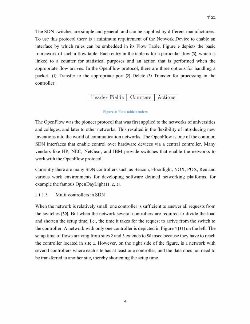
The SDN switches are simple and general, and can be supplied by different manufacturers.
To use this protocol there is a minimum requirement of the Network Device to enable an
interface by which rules can be embedded in its Flow Table. Figure 3 depicts the basic
framework of such a flow table. Each entry in the table is for a particular flow [3], which is
linked to a counter for statistical purposes and an action that is performed when the
appropriate flow arrives. In the OpenFlow protocol, there are three options for handling a
packet: (1) Transfer to the appropriate port (2) Delete (3) Transfer for processing in the
controller.
Figure 3: Flow table headers
The OpenFlow was the pioneer protocol that was first applied to the networks of universities
and colleges, and later to other networks. This resulted in the flexibility of introducing new
inventions into the world of communication networks. The OpenFlow is one of the common
SDN interfaces that enable control over hardware devices via a central controller. Many
vendors like HP, NEC, NetGear, and IBM provide switches that enable the networks to
work with the OpenFlow protocol.
Currently there are many SDN controllers such as Beacon, Floodlight, NOX, POX, Reu and
various work environments for developing software defined networking platforms, for
example the famous OpenDayLight [1, 2, 3].
1.1.1.3 Multi-controllers in SDN
When the network is relatively small, one controller is sufficient to answer all requests from
the switches [30]. But when the network several controllers are required to divide the load
and shorten the setup time, i.e., the time it takes for the request to arrive from the switch to
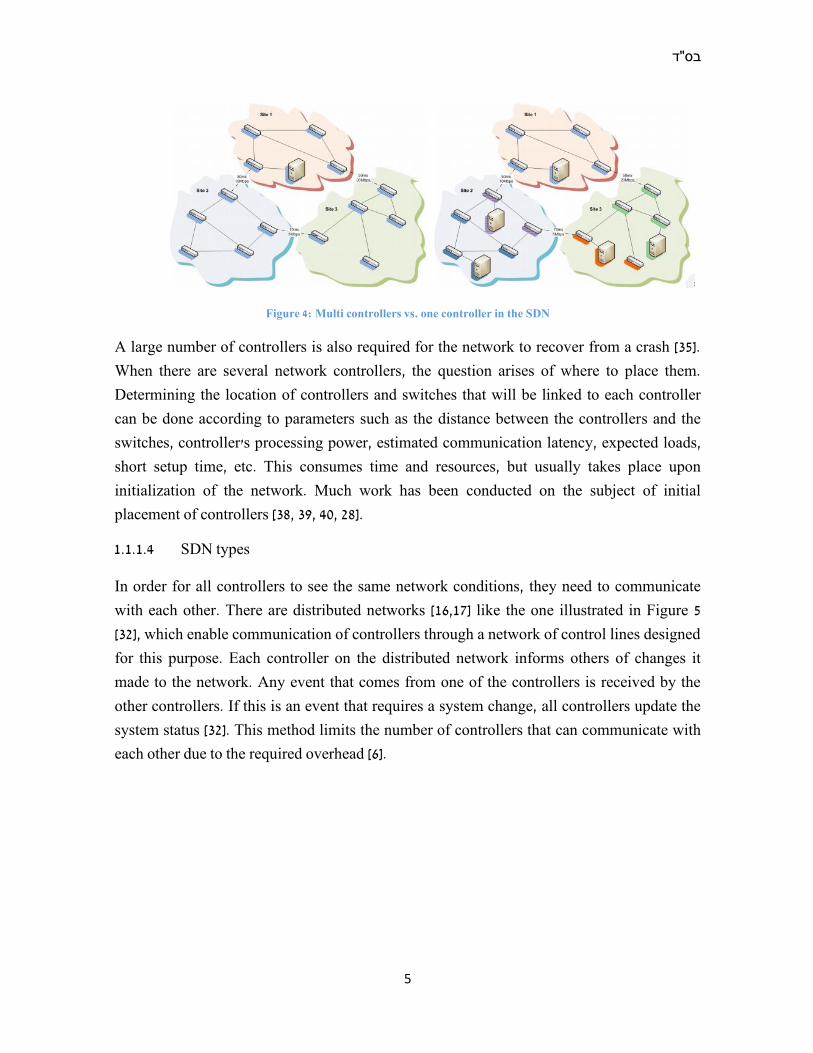
the controller. A network with only one controller is depicted in Figure 4 [32] on the left. The
setup time of flows arriving from sites 2 and 3 extends to 50 msec because they have to reach
the controller located in site 1. However, on the right side of the figure, is a network with
several controllers where each site has at least one controller, and the data does not need to
be transferred to another site, thereby shortening the setup time.
בס"ד
5
Figure 4: Multi controllers vs. one controller in the SDN
A large number of controllers is also required for the network to recover from a crash [35].
When there are several network controllers, the question arises of where to place them.
Determining the location of controllers and switches that will be linked to each controller
can be done according to parameters such as the distance between the controllers and the
switches, controller's processing power, estimated communication latency, expected loads,
short setup time, etc. This consumes time and resources, but usually takes place upon
initialization of the network. Much work has been conducted on the subject of initial
placement of controllers [38, 39, 40, 28].
1.1.1.4 SDN types
In order for all controllers to see the same network conditions, they need to communicate
with each other. There are distributed networks [16,17] like the one illustrated in Figure 5
[32], which enable communication of controllers through a network of control lines designed
for this purpose. Each controller on the distributed network informs others of changes it
made to the network. Any event that comes from one of the controllers is received by the
other controllers. If this is an event that requires a system change, all controllers update the
system status [32]. This method limits the number of controllers that can communicate with
each other due to the required overhead [6].

בס"ד
6
Figure 5: Multi controllers in a distributed network
Another option is to set two levels of controllers. At the top level there is one central
controller termed Super Controller (SC), which is connected to the second level SDN
controllers. The SC is responsible for communication between controllers by collecting and
disseminating information [33,34]. Recently, multi-level architectures have been proposed,
where the lowest level of controllers are linked to the data plane and the other levels are
connected so that one controller in each level is connected to several controllers in the level
below it. In this hierarchical method, a controller in a particular layer can answer a request
that is included in the field of switches that it manages. If the target switch of the request is
not included in the controllers' switches, it passes the request upward in the hierarchy
[37,36].
1.1.2 Load balancing
1.1.2.1 Levels
As networks expand they can contain more data, thus there is need to balance the loads
intelligently. Figure 6 shows two levels in the network where the load balancing operation
can take place. At the bottom level, the requests from hosts should be linked to the switches
in order to avoid overloading the switch. These assignments enable hosts to receive services
in reasonable quality time [19]. At the top level, there are requests that come from switches
to controllers. These requests are generated when the switch needs information from the
controller about the coming data. When the controller is overloaded, its response time for
each request is lengthened, and if the number of requests exceeds the controller's processing
power then requests may be lost. When balancing the requests between controllers, the
distance of each switch from the controller to which it is connected needs to be taken into

בס"ד
7
consideration, both for fast response time and also to reduce the overhead that results from
the control messages sent via the network.
Figure 6: Load balancing levels in SDN systems
Each switch has to be linked to a controller in order to receive the flow rules sent to it. The
more common approach is that each controller has a single default controller to which the
requests are sent. With this approach, the default controller of a switch can be changed, thus
causing all requests that reach the switch to be sent to the new controller. Another approach
is to allow each switch to be linked to several controllers. Thus each switch can transfer
some of the flows to one controller, and other flows to another controller. The distribution of
flows to different controllers enables better load regulation accuracy [9]. The disadvantage
of this method is that, "allocation rules", are required in addition to the standard rules in the
flow table, i.e., the “normal rules” that determine the operation for each flow, in order to
decide which controller will serve the switch if the appropriate flow rule does not exist.
Figure 7 [9] illustrates an example of a Flow Table operating according to this method. As
shown in the flow table, the allocation rules determine the switch, from which the controller
receives a response for a particular flow group. The column "forward to controller" provides
the controller for each flow group.

בס"ד
8
Figure 7: Flow table with controllers for a switch
Most of the existing switches do not support this approach, but perhaps advancements in its
development will transpire in the near future. Nonetheless, there are load balancing methods
that use this approach [9].
1.1.2.2 Periodic balancing
All load balancing approaches divide the timeline into cycles. At each start of the cycle, the
load balancing operation is performed according to the load state as observed in the previous
time cycle. This operation involves new assignments of switches to controllers to balance
the load as much as possible between the controllers, assuming that the load state during the
next cycle will be similar to the load state in the previous cycle. According to this
assumption, the shorter the cycles, the more precise the load balances. Figure 8 illustrates
the division of time into cycles. The run time of the load balancing algorithm, and the
overhead required determines the length of the time cycle.
Figure 8: Cycles in the timeline

בס"ד
9
1.2 Motivation and Goal
Load balancing is done via a central component. In order to ensure that the main component
is not a network bottleneck, algorithms and architecture must be developed that will allow
network scalability for adding controllers without overloading the central component. Our
goal is therefore to reduce the load on the main component without compromising the
efficiency of the load balancing operation.
When the network is large, it may be necessary to run different balancing algorithms on
different parts of the network. In addition, flexibility in replacing the applied algorithms
makes it possible to try different algorithms that have already been proposed in the literature
and those that will be developed in the future. Our goal is therefore to develop architecture
with this flexibility.
The run time of the central element algorithm defines the bound on the time cycle length.
Thus, the more the runtime in the central element increases (i.e., causing a larger time cycle),
the less balance accuracy achieved in the balance operation. This is crucial in dynamic
networks that need to react to frequent changes in loads [11]. Our goal is to reach a short run
time of the cyclic operation, which will enable shortening each cycle of time. Short cycles
enable accuracy in load balancing results. Precise results facilitate good response times by
the controllers. As shown in Table 1, the time complexity of the various methods depends on
the number of controllers and number of switches. When the number of controllers or
switches increases, the time required for the balancing operation increases as well. Our goal
was to find an algorithm with a short time complexity. The methods presented in the table
are discussed in the related work section. The table only specifies the run time of each
method. According to the first three methods the algorithm runs in one component and
depends on the number of controllers and the number of switches. In the Hybrid Flow
method, the algorithm runs in the super controller and other controllers but not
simultaneously, thus the run time of the whole operation also depends on both the number of
controllers and the number of switches. Our goal is to enable an architecture in which the
processing power of the super controller and the controllers that run the balancing
algorithm, are independent of one another, thereby enabling shorter run time and more
precise operation.
בס"ד
10
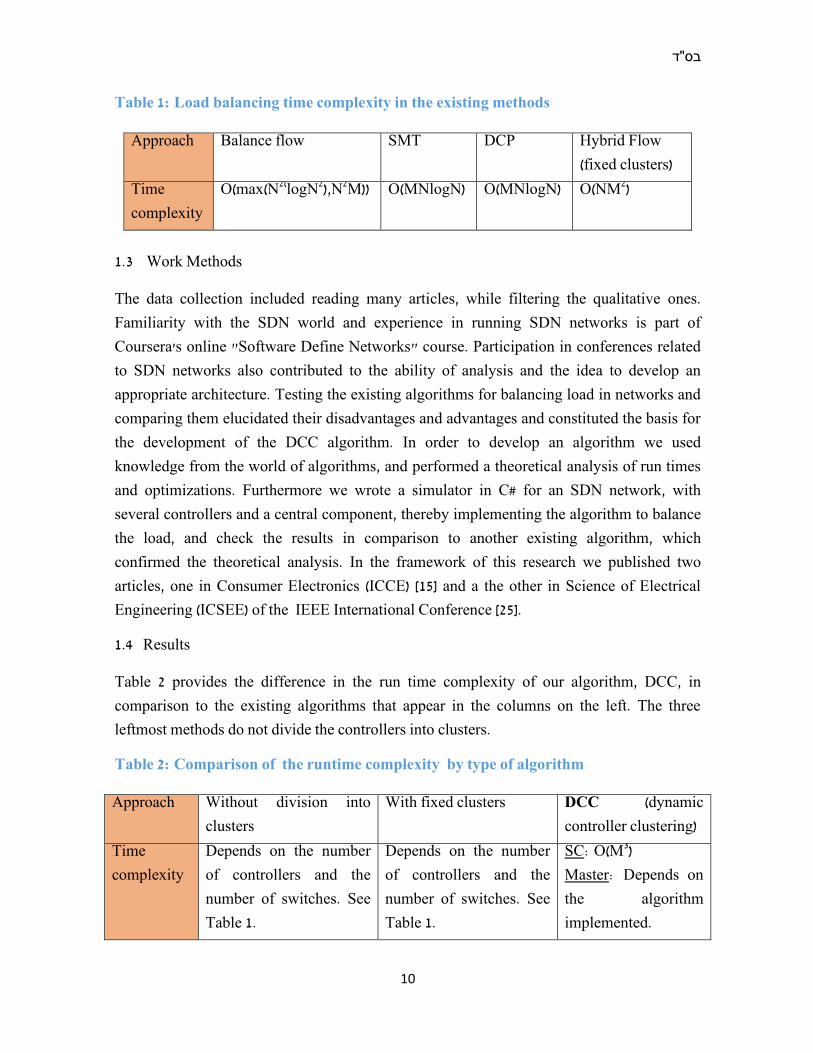
Table 1: Load balancing time complexity in the existing methods
Approach Balance flow SMT DCP Hybrid Flow
(fixed clusters)
Time
complexity
O(max(N2(logN2),N2M)) O(MNlogN) O(MNlogN) O(NM2)
1.3 Work Methods
The data collection included reading many articles, while filtering the qualitative ones.
Familiarity with the SDN world and experience in running SDN networks is part of
Coursera's online "Software Define Networks" course. Participation in conferences related
to SDN networks also contributed to the ability of analysis and the idea to develop an
appropriate architecture. Testing the existing algorithms for balancing load in networks and
comparing them elucidated their disadvantages and advantages and constituted the basis for
the development of the DCC algorithm. In order to develop an algorithm we used
knowledge from the world of algorithms, and performed a theoretical analysis of run times
and optimizations. Furthermore we wrote a simulator in C# for an SDN network, with
several controllers and a central component, thereby implementing the algorithm to balance
the load, and check the results in comparison to another existing algorithm, which
confirmed the theoretical analysis. In the framework of this research we published two
articles, one in Consumer Electronics (ICCE) [15] and a the other in Science of Electrical
Engineering (ICSEE) of the IEEE International Conference [25].
1.4 Results
Table 2 provides the difference in the run time complexity of our algorithm, DCC, in
comparison to the existing algorithms that appear in the columns on the left. The three
leftmost methods do not divide the controllers into clusters.
Table 2: Comparison of the runtime complexity by type of algorithm
Approach Without division into
clusters
With fixed clusters DCC (dynamic
controller clustering)
Time
complexity
Depends on the number
of controllers and the
number of switches. See
Table 1.
Depends on the number
of controllers and the
number of switches. See
Table 1.
SC: O(M3)
Master: Depends on
the algorithm
implemented.

בס"ד
11
In the method to the left of the DCC, called “hybrid flow” the clusters are fixed, while the
DCC algorithm allows dynamic clusters. In the DCC algorithm, the load balancing
operation runs on both the super controller and on one of the controllers within each cluster,
i.e., the Master. Nevertheless, the operations are independent of each other, such that their
run times are calculated separately. The run time of the super controller operation depends
on the number of controllers, while the run time of the operation running on the Masters
depends on the number of controllers and switches belonging to the cluster. All networks
uphold M << N [30], where M is the number of network controllers and N is the number of
switches in the network. The SC operation, performed in regular time cycles, facilitates the
distribution of each time cycle to allow small time periods in which the Master runs on the
cluster. This maximizes utilization of the processing power in the network components, and
shortens the cycle time in which the balancing is performed.
Table 3 presents a comparison of the load balancing results of our method compared to the
fixed clusters method. Each row in the table indicates a particular simulation where the
cycles are the number of time cycles, and times are the number of times the simulation runs
on the networks with different initial loads. Each row contains the results indicating the
differences between clusters' load according to the method of the fixed clusters and our
method of dynamic clusters.
The most right-hand column provides the improvement factor of the dynamic cluster results
compared to the fixed cluster results. On average, dynamic clustering outperforms fix
clustering by a multiplicative factor of 5.
Table 3: Fixed vs dynamic results
Simulation
no.
No. of
controllers
No. of
clusters
Cycles Times Hybrid
Flow - Fix
clustering
Dynamic
clustering
Improvement
Factor
1 16 4 20 961 319.81 61.64 5.2
2 44 11 29 226 999.09 185.33 5.3
3 70 14 18 865 1501.95 267.33 5.6
4 42 14 28 974 1044.48 209.15 4.9
5 30 6 22 203 610 109 5.6

בס"ד
12
2. Related Work
In general, load-balancing methods split the timeline into multiple time slots (TSs) in which
the load balancing algorithms are executed. At the beginning of each TS, a load balancing
algorithm is run based on the input gathered in the previous TS. Therefore, the input is also
assumed to be relevant for the current TS (see Figure 8 above). The load-balancing algorithm
is executed by a central element called the Super Controller (SC). Some of the methods
presented in the literature are adapted to dynamic traffic [14,8]. These methods suggest
changing the number of controllers and their locations, for instance by turning them on and
off in each cycle based on dynamic traffic. In addition to load balancing, other methods [4,8]
deal with additional objectives such as minimal setup time and maximal utilization, which
indirectly help balance loads between controllers. Changing the controllers' locations causes
reassignment of all its switches; consequently, such approaches are designed for networks
where time complexity is not a critical issue.
Other methods [8,9,10] presented in the literature that adapt to dynamic traffic, cause less
noise in the network, whereby the controllers remain fixed and the reassignment of switches
is performed only when necessary. According to these methods the SC runs the algorithm
that reassigns switches according to the dynamic information (e. g., switch requests per
second) it gathers each time cycle from all controllers, and changes the default controllers of
switches according to the loads observed. Note that each controller should publish its load
information periodically to allow SC to partition the loads properly.
In [9] a load balancing strategy called “Balance flow” focuses on controller load balancing
such that (1) the flow-requests are dynamically distributed among controllers to achieve
quick response, and (2) the load on an overloaded controller is automatically transferred to
appropriate low-loaded controllers to maximize controller utilization. This approach
requires each switch to receive service from certain controllers for different flows. The
accuracy of the algorithm is achieved by splitting the switch load between controllers
according to the source and destination of each flow (for example see figure 7).
DCP-GK and DCP-SA, are greedy algorithms for Dynamic Controller Placement (DCP)
introduced by [8]. These algorithms use the Greedy Knapsack (GK) and Simulated
Annealing (SA) for the reassignment phase, respectively, dynamically change the number of
controllers and their locations under different conditions and then reassign switches to
controllers. Contrary to the methods in [8,9], the algorithm suggested by [10] , called
Switches Matching Transfer (SMT) , takes into account the overhead derived from the

בס"ד
13
switch-to-controller and controller-to-switch messages. This algorithm achieves good
results as shown in [10].
In the approaches presented above in this section, all the balancing work is performed by the
SC. Consequently, the load on the SC can be too large causing a bottleneck in the network
and obviously constitute a scalability problem. The load mainly results from gathering
information from all controllers on all the switches on the network, and the balancing
operation being performed only by the central component. This motivated the “Hybrid
Flow” architecture defined and introduced in [18], in which controllers are grouped into
fixed clusters. In order to reduce the load on the SC, the reassignment process is performed
by the controllers in each cluster, where the SC is used only to gather load data and send it
to/from the controllers. “Hybrid Flow” suffers from long runtimes caused by the
dependency that exists between the SC's and other controllers' operations as depicted in
Figure 9. A controller that needs to reassign switches sends a request to the SC which
gathers the data from all controllers and sends it to the controller. After the controller
finishes its reassignments it has to update the SC that maintains the relevant data for other
controllers.
Figure 9: Dependency between two load-balancing levels in Hybrid Flow
Another disadvantage of this method is that each controller makes decisions about the
reassignments to the switches from a local view of the switches that are in its possession
only. This is due to the fact that the information each controller receives from the SC is
general information about the loads on the controllers and not the loads on the switches
associated with them. A decision based on local evidence helps a local problem and does not
always provide an optimal solution for the entire network.
Several works in the field of SDN [12,13,24], deal with hierarchical architectures for SDN
where some layers of controllers use the data plane level. These works, which concentrate
on two primary objectives of response time and overhead, inspired us to take into account
the overhead objective in addition to the response time. Liu et al. [12] discuss the optimal
number of hierarchical layers needed to reduce the response time for a request, but keep the

בס"ד
14
overhead stemming from the number of layers low. Orion's architecture [13] defines the area
controller and domain controller in able to add controllers with a minimum addition to the
control flow and a shorter path in the hierarchical network, which influence the overhead.
Bohle et al. [24] show an implementation of a hierarchical network that enables network
scalability and increases the throughput.

בס"ד
15
3. Model
In this section we introduce the architecture of the network we propose. In the network there
are M controllers, which are denoted C = {C1, C2, C3, ... CM}, and each controller has a set of
switches associated with it. The total number of switches in the network is N. The
controllers are divided into K clusters, such that there are M / K controllers in each cluster.
The processing power, which relates to the number of requests it can support per second, per
controller is P. In each cluster there is one controller called “Master”, which is responsible
for balancing the loads within the cluster. Each controller has the address of its Master, and
each Master controller has the list of controllers’ addresses connected to it, denoted
ClusterVector (CV). The master controller receives information from the controllers
belonging to its cluster, with respect to the loads they experience, and accordingly balances
the loads between them. The relationship between the clusters is done by a single controller,
SuperController (SC), linked to all the Master controllers by a list of Master controller
addresses stored in it called the MastersVector (MV). The SC collects the master controller's
information about the load experienced by all controllers, and then repartitions the
controllers into clusters. In addition to the redistribution of the clusters, SC can modify the
Master controllers, i.e. the MV. According to the new MV, the Masters are updated by
means of the SC in their updated CVs.
Figure 10 depicts two different examples of clustering. Figure 10.a. shows that SC
communicates with all the MCs, i.e. c3, c6 and c12. Controller c3 is the master of
},,,{ 93211 ccccG . Controller c6 is the master of
},,,{ 47652 ccccG and Controller c12 is the
master of},,,{ 12111083 ccccG
. In Figure 10.b. c4 moved from group G2 to group G1, c9
moved from group G1 to group G3 and c8 moved from group G3 to group G2. In group G1,
after all the replacements c2 became the master.
Figure 10: An example of dynamic clustering

בס"ד
16
The Masters' internal balancing operations in clusters and the SC's overall balancing are
independent of one another and can therefore be performed simultaneously in the various
network components. The super-level balancing operation, which is a division into dynamic
clustering by the SC, is denoted "clustering" while the internal operation performed by the
master controller, which actually reconnects switches to different controllers, is denoted
"reassignment". The two actions together create the dynamic load balancing and are adapted
to the network load state. On the one hand there is a cluster change so that the cluster level is
balanced, and on the other hand within each cluster there is a balance between the loads. As
a result, these operations are balanced in all controllers.
The architecture, therefore, defines three levels: the SC level, the Masters' level, and the
standard level of controllers. We call this architecture the Dynamic Cluster Flow (DCF) due
to the fact that its main idea is the dynamic distribution of the clusters according to the load,
which is measured by the average flow per controller.
As depicted in Figure 12, the timeline is divided into time units, where a “clustering”
balancing algorithm that updates the CVs is run at the beginning of each time unit. Each unit
in the timeline is divided into sub-units, where the “reassignment” balancing algorithm is
run at the beginning of each sub-unit. Nonetheless the “reassignment” algorithm is run
concurrently by several controllers, i.e., by the Masters, each in its own cluster, on a limited
number of controllers. Hence a short run time is achieved, which can significantly shorten
the cycle time and thus result in more accurate balancing results.
Figure 11: operations of the SC and the Masters when clusters are dynamic

בס"ד
17
4. DCC Problem Formulation
4.1 Notation
We consider a control plane with M controllers, denoted by },...,,{ 21 MCCCC where iC
is a single controller and its processing power is denoted P , which stands for the number of
requests per second that it can handle. We use dij to denote the distance (number of hops)
between iC and jC. We use iG to denote the ith cluster and
},...,,{ 21 kGGGG , the set of all
clusters. We assume that M / K is an integer and is actually the number of controllers per
cluster. Thus, the size of the CV is M/K. Y denotes a matrix, handled by SC, which consists
of the matching of each controller to a single cluster. Each column of Y represents a cluster
and each row a controller. Therefore, Y is a binary KM matrix as follows:
.)(,1)(,0
1{)(
1
1
1
1 ktYandtYthatsuchelse
GCtY
M
j
jiKi
K
i
jiMj
ij
ji
The load of controller j in time slot t is denoted 𝑙(𝑡)𝑗. This information arrives from the
controllers that calculate the average of requests per second from all their switches in time
slot t. CVLi denotes the Cluster Vector Load of Masteri. The super controller also contains
the addresses of the masters for each cycle in the Master Vector (MV). Table 2 summarizes
the key notations for ease of reference.
Table 4: Key notations
Symbol Semantics
jC jth controller
iG ith cluster
P the number of requests a controller can handle per second
𝑑𝑖𝑗 Minimal hop distance between Ci and Cj
jitY )( jitY )( =1 if jth controller is in cluster i in time slot t, else jitY )( =0
𝑙(𝑡)𝑗 Controller load - Average flow request of jth controller per second in
time slot t
SC Super Controller – collects controllers' loads from masters and re-
clustering

בס"ד
18
To define the problem of the “Clustering” for the high level of the load balancing
operation we defined two aspects; we sought the minimal differences between
clusters' loads and the minimal distances between controllers in each cluster. These
two aspects enabled us to decrease the response time and the overhead, respectively,
in the lowest level of the load balancing, i.e., “Reassignment”. The next two sections
define these two aspects.
4.2 Clusters' Load Differences
To achieve balanced clusters, the gaps between their loads must be narrowed. A
cluster load is the sum of the controllers' average loads in it, as follows:
M
j
jiji tYtlt1
)()()( (1)
Where i is the cluster number and M is the number of controllers.
To measure how much a cluster load is far from other clusters' loads, we used the
global cluster's load average:
k
tl
Avg
M
j
j
)(
(2)
Where, k is the number of clusters. We first defined the distance of a cluster from the
global average Avg as:
|)()( Avgtt ii (3)
Then, in a second step, we defined a metric that measures the total load difference
between clusters as follows:
K
t
t
K
i
i 1
)(
)(
(4)
Where if 0)( t all clusters' loads equal the global average, which means that the
sum of the load distances from the global average (i.e., the difference) is equal to
zero.
4.3 Controllers' Distances
The greater the distance between controllers belonging to the same cluster, the
greater the communication overhead between them. In order to prevent too much
overhead we wanted to form clusters such that the controllers within the same cluster
are not far from each other. For that purpose we defined a constraint on the maximal
distance allowed which we denote Cnt .

בס"ד
19
The maximal distance between controllers within the same cluster is defined as
follows:
jcicijMjikc
tYtYdt )()(maxmax)(,11
(5)
Where c is the cluster number, and i , j are the controllers in c cluster. To obtain a
constraint on the distance corresponding to the network data, we set the
"maxDistance" to the lower limit on the constraint value, i.e., the constraint could
not be smaller than it. To enable a relaxation of this constraint an "offset" could be
added, and the final maximal constraint, which is adjusted to the network's distance
data is:
Cnt maxDistance + offset (6)
4.4 Dynamic Controllers' Clustering
Our goal is to minimize )(t (Eq. 4) while finding the matrix Y(t) and fulfilling the distance
constraint (Eq. 6). Therefore, the problem formulation is as follows:
jiij
K
i
ji
M
j
ji
tY
Cntt
jtY
iK
MtY
ts
t
,1,0)(
)9()(
)8(,1)(
)7(,)(
..
)(min
Equation 7 ensures that each cluster has exactly M/K controllers at a given time. Equation 8
ensures that each controller is assigned to exactly one cluster at a time and Equation 9
concerns the controller-controller distance in a cluster.
In other words, the minimization problem defined above is: Given a connected graph G =
(V, E) with a weight function w: V → Z+ and K ≥ 2 is a positive integer. For X ⊆ V, let w(X)
denote the sum of the weights of the vertices in X. For the problem of G we need to find a q-
partition P = (V1, V2, . . . , Vk) of V such that G[Vi] is connected (1 ≤ i ≤ q) and P maximizes
min{w(Vi) : 1 ≤ i ≤ q} and | V1 | = |V|/K.
In this problem, we address two aspects of the network, namely, the distance between the
controllers within the same cluster and the load differences between the clusters, which
בס"ד
20
influence the overhead, and the response time, respectively. Regarding the distance aspect,
the problem is a variant of a k-Center problem [20], where we look for the center's nodes in
the network that are within distances which fulfil the distance constraint to build the clusters
around them, in order to obtain a value for maxDistance that would be relevant to the
network's distance data. When we consider the second aspect, i. e., the load differences
between clusters, in addition to the distance constraint, the problem is a variant of a
coalition-formation game problem [21], where the network structure and the cost of
cooperation play major roles. These two general problems are NP-Complete because finding
an optimal partition requires iterating over all the partitions of the player set, where the
number of these partitions grows exponentially with the number of players, and is given by a
value known as the Bell Number. Hence, finding an optimal partition in general is
computationally intractable and impractical (unless P = NP).
In this paper, we propose an approximation algorithm to solve this problem. We adapt the
K-Center problem solution for initial clustering, and use game theoretic techniques to satisfy
our objective function with the distance constraint.
בס"ד
21
5. Dynamic Controller Clustering Algorithm
In this section, we divide the DCC problem into two phases and present our solutions for
each of them. In the first phase, we define the initial clusters. We show some possibilities for
the initialization that refer to distances between controllers and load differences between
clusters. In the second phase, we improve the results. We further reduce the differences of
cluster loads without violating the distance constraint by means of our replacement
algorithm. We also discuss the connections between these two phases, and the advantages of
using this two-phase approach for optimizing the overall performance.
5.1 Phase 1: Initial Clustering
The aim of initial clustering is to enable the best start that provides the best result for the
second phase. Thus, we observe two options for initialization. The first option is where only
the overhead is important and requires that a minimum distance value be set for the clusters,
which determines the maximum distance between the controllers in the same cluster. The
second option is where only the clusters’ loads is important and requires that a minimum
difference value be set for the clusters ensure that the loads of the clusters are similar
5.1.1 Initial clustering with the distance constraint
Most of the control messages concerning the cluster load balancing operation are generated
because of the communication between the controllers and their MC. Thus, we use the K-
Center problem solution to find the MCs [20, 22, 23]. In this problem, 𝐶 = {𝐶1, … , 𝐶𝑘} is the
center's group and 𝑃 = {𝑝1, … , 𝑝𝑀} contains M controllers. We define
𝑃𝐶 = (𝑑(𝑝1, 𝐶) , 𝑑(𝑝2, 𝐶) , … , 𝑑(𝑝𝑀, 𝐶)), where the ith coordinate of 𝑃𝐶 is the distance of
𝑝𝑖 to its closest center in C. The K-Center input is: A set 𝑃 of M points and integer number
k, where M ∈ ℕ , 𝑘 < 𝑀. The goal is to find a set of k points 𝐶 ⊆ 𝑃 such that the maximum
distance between a point in P and its closest point in C is minimized. The network is a
complete graph, and the distance definition [see Table 4] satisfies the triangle inequality.
Thus, we can use an approximate solution to the K-Center problem to find MCs. Given a set
of centers, C, the k-center clustering price of P by C is ‖PC‖∞ = maxp∈P d(p, C). Algorithm
1 is an algorithm similar to the one used in [22]. This algorithm computes a set of k centers,
with a 2-approximation to the optimal k-center clustering of P, i.e., ‖𝑃𝐾‖∞ ≤ 2𝑜𝑝𝑡∞(𝑃, 𝑘)
with O(Mk) time and O(M) space complexity [22].

בס"ד
22
Algorithm 1 : Find masters by 2-approximation greedy k-center solution
In Line 1 the algorithm chooses a random controller as the first master. In Line 2 the
algorithm computes the distances of all other controllers from the master chosen in line 1.
Lines 3-4 are for the second master chosen, which is the farthest controller from the first
master. In the loop, in row 5, in each iteration, another master is added to the collection by
calculating the controller located in the farthest radius of all controllers already included in
the master group. After )K-2( iterations in line 6 the set of masters is ready. After Algorithm
1 finds K masters, we partition controllers between the masters by keeping the number of
controllers in each group under M/K as illustrated in Heuristic 1 below.
Input: set 𝑃 = {𝑝1, … , 𝑝𝑛} contains M controllers, controller-to-controller matrix distances Output: set of master 𝐶 = {𝐶1, … , 𝐶𝑘}, 𝐶𝑃
1. Pick an arbitrary point pi from P pi= 𝑐1̅, and set 𝐶1 = {𝑐1̅}. 2. For every point 𝑝 ∈ 𝑃 compute the distance 𝑑1[𝑝] ≔ 𝑑(𝑝, 𝑐1̅) from
𝑐1̅. 3. Consider the worst point served by 𝐶1 – which is the point that
realizes 𝑟1 = max𝑝∈𝑃 𝑑1[𝑝].
4. Let 𝑐2̅ denote this point and add it to 𝐶1 , resulting in the set 𝐶2.
5. In each iteration i = 1,2,…,k do: //Compute the quantity for each point 𝑝 ∈ 𝑃
a. 𝑑𝑖−1[𝑝] = 𝑑(𝑝, 𝐶𝑖−1) = min𝑐̅∈𝐶𝑖−1𝑑(𝑝, 𝑐̅)
//Compute the radius of the clustering
b. 𝑟𝑖−1 = ‖𝑃𝐶𝑖−1‖
∞= max𝑝∈𝑃 𝑑𝑖−1[𝑝] = max𝑝∈𝑃 𝑑(𝑝, 𝐶𝑖−1)
c. Let 𝑐�̅� denote the point realizing it. d. Add 𝑐�̅� to 𝐶𝑖−1 to form the new set 𝐶𝑖 ≔ 𝐶𝑖−1 ∪ {𝑐�̅�}.
Repeat this process k times.
6. Return the final set 𝐶𝑘of the masters
בס"ד
23
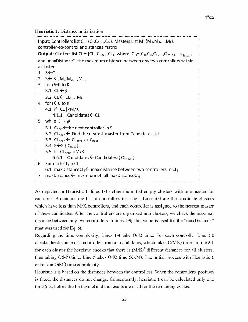
Heuristic 1: Distance initialization
As depicted in Heuristic 1, lines 1-3 define the initial empty clusters with one master for
each one. S contains the list of controllers to assign. Lines 4-5 are the candidate clusters
which have less than M/K controllers, and each controller is assigned to the nearest master
of these candidates. After the controllers are organized into clusters, we check the maximal
distance between any two controllers in lines 1-5; this value is used for the “maxDistance”
(that was used for Eq. 6).
Regarding the time complexity, Lines 1-4 take O(K) time. For each controller Line 5.2
checks the distance of a controller from all candidates, which takes O(MK) time. In line 6.1
for each cluster the heuristic checks that there is (M/K)2 different distances for all clusters,
thus taking O(M2) time. Line 7 takes O(K) time (K<M). The initial process with Heuristic 1
entails an O(M2) time complexity.
Heuristic 1 is based on the distances between the controllers. When the controllers' position
is fixed, the distances do not change. Consequently, heuristic 1 can be calculated only one
time (i.e., before the first cycle) and the results are used for the remaining cycles.
Input: Controllers list C = {C1,C2,…,CM}, Masters List M={M1,M2,…,Mk}, controller-to-controller distances matrix
Output: Clusters list CL = {CL1,CL2,..,CLk} where CLi={C1i,C2i,C3i,…,C(M/K)i} ki1 ,
and maxDistance”- the maximum distance between any two controllers within a cluster. 1. SC 2. S S-{ M1,M2,…,Mk } 3. for i0 to K
3.1. CLi
3.2. CLi CLi Mi 4. for i0 to K
4.1. if |CLi|<M/K 4.1.1. Candidates CLi
5. while S
5.1. Cnextthe next controller in S 5.2. CLnear Find the nearest master from Candidates list 5.3. CLnear CLnear Cnext 5.4. SS-{ Cnext } 5.5. If |CLnear|=M/K
5.5.1. Candidates Candidates-{ CLnear } 6. For each CLi in CL
6.1. maxDistanceCLi max distance between two controllers in CLi 7. maxDistance maximum of all maxDistanceCLi
בס"ד
24
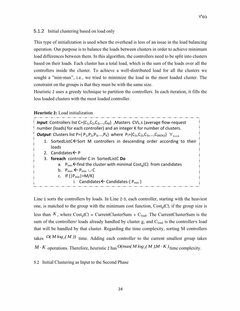
5.1.2 Initial clustering based on load only
This type of initialization is used when the overhead is less of an issue in the load balancing
operation. Our purpose is to balance the loads between clusters in order to achieve minimum
load differences between them. In this algorithm, the controllers need to be split into clusters
based on their loads. Each cluster has a total load, which is the sum of the loads over all the
controllers inside the cluster. To achieve a well-distributed load for all the clusters we
sought a ”min-max”, i.e., we tried to minimize the load in the most loaded cluster. The
constraint on the groups is that they must be with the same size.
Heuristic 2 uses a greedy technique to partition the controllers. In each iteration, it fills the
less loaded clusters with the most loaded controller.
Heuristic 2: Load initialization
Line 1 sorts the controllers by loads. In Line 2-3, each controller, starting with the heaviest
one, is matched to the group with the minimum cost function, Costg(C), if the group size is
less than K , where Costg(C) = CurrentClusterSum + Cload. The CurrentClusterSum is the
sum of the controllers' loads already handled by cluster g, and Cload is the controller's load
that will be handled by that cluster. Regarding the time complexity, sorting M controllers
takes ))M(logM(O 2 time. Adding each controller to the current smallest group takes
KM operations. Therefore, heuristic 2 has )KM),M(logM(max(O 2 time complexity.
5.2 Initial Clustering as Input to the Second Phase
Input: Controllers list C={C1,C2,C3,…,CM} ,Masters CVLi s (average flow-request number (loads) for each controller) and an integer K for number of clusters.
Output: Clusters list P={ P1,P2,P3,…,PK} where Pi={C1i,C2i,C3i,…,C(M/K)i} ki1
1. SortedListCSort M controllers in descending order according to their loads
2. Candidates P 3. foreach controller C in SortedListC Do
a. Pminfind the cluster with minimal Costg(C) from candidates b. Pmin Pmin C c. If (|Pmin|=M/K)
i. Candidates Candidates-{ Pmin }

בס"ד
25
The two types of initialization, namely “distance” and “load”, mentioned above are used as
an input for the second phase.
The distance initialization process (Heuristic 1) ensures that we start with clustering that will
meet a distance constraint. The output of this process is an initial clustering and
“maxDistance”, where the clustering meets the “maxDistance” constraint. An offset is
added to the “maxDistance” constraint to create the final Cnt (Eq. 6). This clustering needs
to be updated to improve the differences between the clusters' loads. Thus, this first phase is
mandatory to fulfill the distance constraint.
The load initialization process (Heuristic 2) is used when there is no distance constraint. In
such cases, this process is not essential to solve the problem, but it can accelerate the
convergence of the second phase.
In the second phase, we apply the coalition game theory [21]. In a coalition game, there are
participants in each coalition. We can define a rule to transfer participants from one
coalition to another. The outcome of the initial clustering process is a partition denoted
defined on a set C that divides C into K clusters with M/K controllers for each cluster. Each
controller is associated with one cluster. Hence, the controllers that are connected to the
same cluster can be considered participants in the coalition. Thus, the clustering obtained
from the first phase is suitable for use in the coalition game theory to further improve our
results.
5.3 Phase 2: Decrease Load Differences using a Replacement Rule
We now leverage the coalitional game theory to improve the performance of the controllers
clustering considering load differences between groups. A coalition structure is defined by a
sequence },...,,,{ 321 lBBBBB
where each iB is a coalition. In general, a coalition game is
defined by the triplet ),,( BvN , where v is a characteristic function, N are the elements that
need to be grouped and B is a coalition structure that partitions the N elements [21]. In our
problem the M controllers are the elements, G is the coalition structure, where each group
of controllers iG is a coalition. Therefore, in our problem we can defined the coalition game
by the triplet ),,( GvM where )(tv . The second phase can be considered a coalition
formation game. In a coalition formation game each element can change its coalition based
on the utility it can gain. Thus, a controller may be transferred to another cluster with a

בס"ד
26
lower global load than its current cluster. We use itsm )( to denote the safety margin of
cluster i, which specifies the load that can still be transferred to a particular cluster without
exceeding its capacity. This is derived as follows:
K
c
M
i
M
j
jjcici tltYtYPKtsm )()()()(
In order to keep the cluster size (i.e., the same number of controllers in each cluster), we
exchange controllers, such that each controller which is moved must have a substitute. To
determine whether, after the replacement, the )(t (Equation 4) was reduced or not, we
define the Replacement Value (RV) as follows:
elsetttt
AvgtAvgt
AvgtAvgt
Cntt
CntbaccRV
oldoldnewnew
oldold
oldold
baba
ba
ba
new
ji
))()(())()((
))((&))((0
)))((&))((0
)(0
{),,,,(
(10)
Each replacement involves two controllers ic and jc
with loads itl )( and jtl )(
,
respectively, and two clusters a and b with loads aL and bL
, respectively. We use the
notations ”old” and “new” to indicate a value before and after the replacement.
When Cntt new )(
(see equations 5 and 6), the controllers, after the replacement, are
organized into clusters such that the maximum distance between controllers within a
particular cluster exceeds the distance constraint Cnt . In this case, the value of the RV is set
to zero, because the replacement is not relevant at all.
When )))((&))(( AvgtAvgt oldold ba
or
))((&))(( AvgtAvgt oldold ba
(see
equation 2 and 3), there are two options as follows: One option is when the loads of the two
clusters remain above average or both below average, even after the replacement. In this
situation, oldt)( = newt)(
(i.e., )(t
before and after the replacement; see equation 4). The
second option is when one of the clusters moves to another side of the average. In such
cases, we have oldnew tt )()( . With both options, oldt)(
does not improve and therefore
the RV is set to zero.
Figure 12 and Figure 13 provide an illustration of these two options. The dotted line denotes
the average of all clusters.

בס"ד
27
Figure 12: Clusters loads after replacement on the same side with reference to the average
In Figure 12, the sum of the loads’ distances from the global average, before the replacement
is x+y. After the replacement the sum isyxtltlytltlx jiji ))()(())()(((
. In
the other symmetrical options, the result is the same.
Figure 13: Clusters' loads after replacement on different sides with reference to the average
In Figure 13 the sum of distances from the global average, before the replacement is x+y,
and this sum after the replacement isyxytltltltlx jiji ))()(())()((
. In the
other symmetrical options, the result is the same.
In equation 10, If none of the first three conditions are met, RV is calculated by
))()(())()(( oldoldnewnew babatttt
, a value that can be greater than or less than zero.
Using the RV, we define the following “Replacement Rule”:

בס"ד
28
Definition 1. Replacement Rule. In a partition , a controller ic has incentive to replace its
coalition a with controller jc from coalition b (forming the new coalitions
ji
oldnew ccaa )\( and ij
oldnew ccbb )\( ) if it satisfies both of the following:
(1) The two clusters newa and
newb that participate in the replacement do not exceed their
capacity K*P. (2) The RV satisfies: 0),,,( baccRV jidis (RV defined in Equation 10)
In order to minimize the load difference between the clusters we iteratively find a pair of
controllers with minimum RV, which then implement the corresponding replacement. This
is repeated until all RV’s are larger than or equal to zero: 0),,,( baccRV ji .
Algorithm 2 details the replacement procedure.
Algorithm 2: Replacement Procedure
Regarding the time complexity of lines 1-4, i.e., find the best replacement, takes:
))1((...)2()1( KKK
M
K
MK
K
M
K
MK
K
M
K
M)(
2
)1(
2
)1( 22
2
2
MOK
KMKK
K
M
time.
Line 6 invokes the replacement within O(1) time. Since in each iteration the algorithm
chooses the best solution, there will be a maximum of M/2 iterations in the loop of lines 1-5.
Thus, in the worst case Algorithm 2 takes an O(M3) time complexity. In practice, the number
of iterations is much smaller, as can be seen in the simulation section.
5.4 Dynamic Controller Clustering Full Algorithm
Input: Clusters list P={ P1,P2,P3,…,PK} where Pi={C1i,C2i,C3i,…,C(M/K)i} ki1 ,
distance constraint Cnt
Output: Clusters list P={ P1,P2,P3,…,PK} where Pi={C1i,C2i,C3i,…,C(M/K)i} ki1
1. bestVal0; 2. bestVal the minimal ),,,,( CntbaccRV ji for each two controllers
belongs to different clusters in P 3. ),,,( bacc ji bestVal replacement details (controllers and clusters
participants) 4. If ),,,,( CntbaccRV ji < 0
a. invoke the replacement ),,,( bacc ji
b. repeat to 1 5. else
a. return P

בס"ד
29
Now we present the algorithm that includes the two stages of initialization and replacement,
in order to obtain clusters in which the loads are balanced.
DCC Algorithm
The DCC Algorithm runs the appropriate initial clustering, according to a Boolean flag
called “constraintActive”, indicating whether the distance between the controllers should be
considered or not )Line 1(. If the flag is true, the “distance initialization” procedure
)Heuristic1( is called )line 1.b(. Using the “maxDistance” output from Heuristic 1, the DCC
calculates the Cnt = maxDistance + offset (Line 1.c). Using the partition and Cnt outputs, the
DCC runs the “replacement procedure” )Algorithm2( )Line 1.d(.
The DCC can run the second option without any distance constraint (Line 2). In Line 2.e it
chooses the best solution in such cases, (referring to the minimal load differences) from the
following three options:
(1) Partition by loads only (Line 2.b);
(2) Start partition by loads and improve with replacements (Line 2.c)
(3) Partition by replacements only (using the previous cycle partition) (Line 2 d).
Input: Network nt with a Controllers list C = {C1,C2,…,CM}, and distances between controllers. K and M for the number of clusters and controllers, respectively, constaintActive to indicate that it meets the controller-to-controller distance constraint, offset to calculate the distance constraint (optional).
Output: Clusters list P={ P1,P2P3,…,PK} where Pi={C1i,C2i,C3i,…,C(M/K)i} ki1
1. If (constaintActive = true) a. MastersAlgorithm1(nt) b. (initialDistanceClusters,maxDistance)Heuristic1(C,Masters) c. CntmaxDistance+offset d. finalPartitionAlgorithm2(initialDistanceClusters,true,Cnt)
2. else a. initialStructureCluster structure from the previous cycle b. initialLoadsOnly Heuristic2(c) c. initialWithReplacementAlgorithm2(initialLoadsOnly,false) d. ReplacementOnly Algorithm2(initialStructure,false) e. finalPartition best solution from(initialLoadsOnly,
initialWithReplacement, ReplacementOnly) 3. return finalPartition

בס"ד
30
Regarding the time complexity, DCC uses heuristic 1, heuristic 2, algorithm 1 and algorithm
2, thus it has a )( 3MO time complexity.
5.5 Optimality Analysis
In this section, our aim is to prove how close our algorithm is to the optimum. Because the
capacity of controllers is identical, the minimal difference between clusters is achieved
when the controllers' loads are equally distributed among the clusters, where the clusters'
loads are equal to the global average, namely 0)( t . Since in the second phase, i.e., in the
replacements, the DCC full algorithm is the one that sets the final partition and therefore
determines the optimality, it is enough to provide proof of this.
As mentioned before, the replacement process is finished when all RVs 0, at which time
any replacement of any two controllers will not improve the result. Figure 14 shows the
situation for each two clusters at the end of the algorithm.
Figure 14: The loads of each two clusters at the end of all replacements
For each two clusters, where the load of one cluster is above the general average and the
load of the second cluster is below the general average, the following formula holds:
bcactltlLLtt jijibaba ,),)()(()()(
. (11)
We begin by considering the most loaded cluster and the most under-loaded cluster. When
the cluster size is g, we define X1 to contain the lowest g / 2 controllers, and X2 to contain

בס"ד
31
the next lowest g / 2 controllers. In the same way, we define Y1 to contain the highest g / 2
controllers and Y2 to contain the next highest g / 2 controllers.
In the worst case, the upper cluster has the controllers from the Y1 group and the lower
cluster has the controllers from the X1 group. Since the loads of the clusters are balanced,
one half of the controllers in the upper cluster are from X2, and the other half of controllers
in the lower cluster are controllers from Y2.
According to Formula 11, we can take the lowest difference between a controller in the
upper cluster and a controller in the lower cluster to obtain a bound on the sum of the
distance of loads of these two clusters from the overall average. The sum of distances from
the overall average of these two clusters is equal to or smaller than the difference between
the two controllers, i.e., between the one with the lowest load of the g most loaded controller
and the one with the highest load of the g lowest controllers.
))()(()()( _______ smallertngbiggerthgloadedundermostloadedmost tltltt (12)
The bound we received (Eq. 12), for the two most distant clusters, can now be multiplied by
k / 2, in order to determine a bound for )(t . However, to obtain a more stringent bound, we
can consider bounds of other cluster pairs, and summarize all bounds as follows:
𝑑𝑖𝑓𝑓𝑒𝑟𝑒𝑛𝑐𝑒𝐵𝑜𝑢𝑛𝑑 ≤ ∑ (𝑠𝑜𝑟𝑡𝐿𝑖𝑠𝑡(𝑀−𝑖𝑔) − 𝑠𝑜𝑟𝑡𝐿𝑖𝑠𝑡𝑖𝑔)𝑀
2𝑔⁄
𝑖=1 (13)
The 𝑠𝑜𝑟𝑡𝐿𝑖𝑠𝑡 indicates the load list of the controllers sorted in ascending order, 𝑀 the
number of controllers, and 𝑔 the cluster size.
בס"ד
32
6. Results
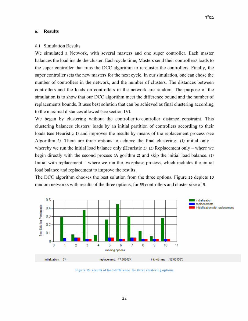
6.1 Simulation Results
We simulated a Network, with several masters and one super controller. Each master
balances the load inside the cluster. Each cycle time, Masters send their controllers' loads to
the super controller that runs the DCC algorithm to re-cluster the controllers. Finally, the
super controller sets the new masters for the next cycle. In our simulation, one can chose the
number of controllers in the network, and the number of clusters. The distances between
controllers and the loads on controllers in the network are random. The purpose of the
simulation is to show that our DCC algorithm meet the difference bound and the number of
replacements bounds. It uses best solution that can be achieved as final clustering according
to the maximal distances allowed (see section IV).
We began by clustering without the controller-to-controller distance constraint. This
clustering balances clusters' loads by an initial partition of controllers according to their
loads (see Heuristic 1) and improves the results by means of the replacement process (see
Algorithm 2). There are three options to achieve the final clustering: (1) initial only –
whereby we run the initial load balance only (Heuristic 2). (2) Replacement only – where we
begin directly with the second process (Algorithm 2) and skip the initial load balance. (3)
Initial with replacement – where we run the two-phase process, which includes the initial
load balance and replacement to improve the results.
The DCC algorithm chooses the best solution from the three options. Figure 16 depicts 10
random networks with results of the three options, for 55 controllers and cluster size of 5.
Figure 15: results of load difference for three clustering options
בס"ד
33
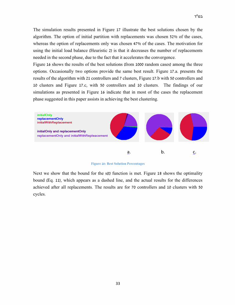
The simulation results presented in Figure 17 illustrate the best solutions chosen by the
algorithm. The option of initial partition with replacements was chosen 52% of the cases,
whereas the option of replacements only was chosen 47% of the cases. The motivation for
using the initial load balance (Heuristic 2) is that it decreases the number of replacements
needed in the second phase, due to the fact that it accelerates the convergence.
Figure 16 shows the results of the best solutions (from 1000 random cases) among the three
options. Occasionally two options provide the same best result. Figure 17.a. presents the
results of the algorithm with 21 controllers and 7 clusters, Figure 17.b with 50 controllers and
10 clusters and Figure 17.c, with 50 controllers and 10 clusters. The findings of our
simulations as presented in Figure 16 indicate that in most of the cases the replacement
phase suggested in this paper assists in achieving the best clustering.
Figure 16: Best Solution Percentages
Next we show that the bound for the s(t) function is met. Figure 18 shows the optimality
bound (Eq. 11), which appears as a dashed line, and the actual results for the differences
achieved after all replacements. The results are for 70 controllers and 10 clusters with 50
cycles.

בס"ד
34
Figure 17: Difference bound and the final difference
As the number of controllers increases, the distance between the difference bound and the
actual difference increases. This is because the bound is calculated according to the worst
case scenario. Figure 19 shows the increase in distance between the actual distance and the
distance bound when the number of controllers increases. The results are for 5 controllers in
a cluster with 50 cycles.
Figure 18: Distance between the difference bound and the actual difference
בס"ד
35
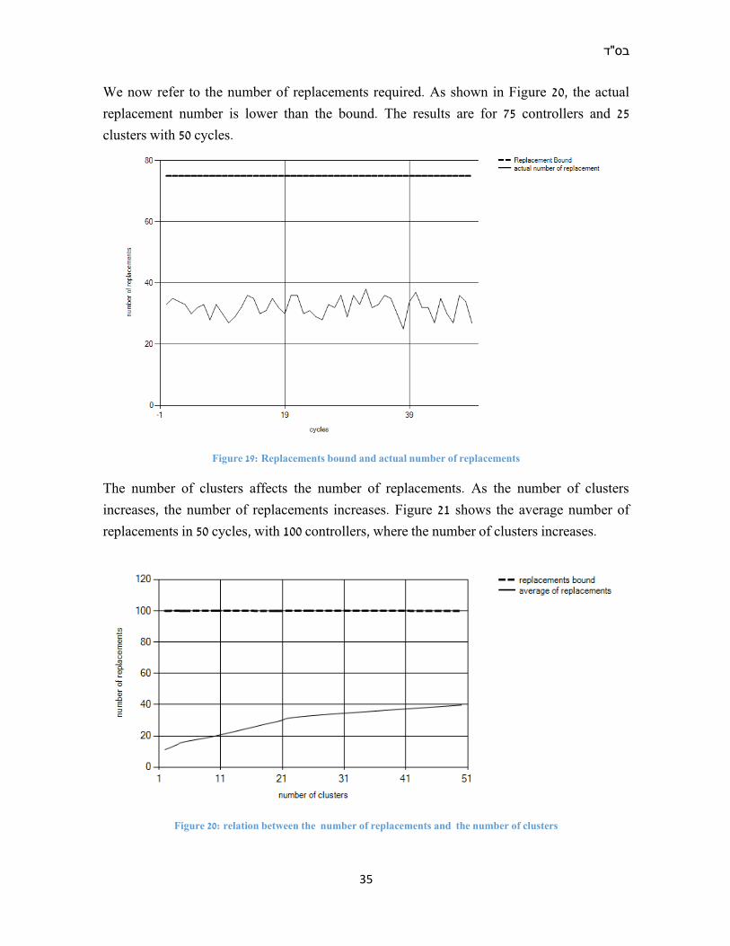
We now refer to the number of replacements required. As shown in Figure 20, the actual
replacement number is lower than the bound. The results are for 75 controllers and 25
clusters with 50 cycles.
Figure 19: Replacements bound and actual number of replacements
The number of clusters affects the number of replacements. As the number of clusters
increases, the number of replacements increases. Figure 21 shows the average number of
replacements in 50 cycles, with 100 controllers, where the number of clusters increases.
Figure 20: relation between the number of replacements and the number of clusters

בס"ד
36
As noted, the initialization of step 1 in the DCC algorithm reduces the number of
replacements required in step 2. Figure 22 depicts the number of replacements required, with
and without the initialization of step 1. The results are for 75 controllers and 15 clusters with
50 cycles.
Figure 21: Number of replacements with and without initialization of step 1
When a controller-to-controller maximal distance constraint is important, there is a lower
bound on the maximal distance. By adding this lower bound to the offset defined by the
user, an upper bound called "Cnt" is calculated (Eq. 6). Figure 23 shows the final maximal
distance that remains within the upper and lower bounds. The results are for 50 controllers
and 5 clusters with 30 cycles.

בס"ד
37
Figure 22: Maximal distance between lower and upper bounds
Finally, we compare our method of dynamic clusters with different method of fixed clusters.
As a starting point, the controllers are divided into clusters according to the distances
between them (Heuristic 1). In each time cycle, the clusters are rearranged according to the
controllers’ loads in the previous time cycle. The change in the load status from cycle to
cycle is defined by the following transition function:
f(n) = {max ((l(t)i + random(range), P) random(0,1) = 1
max ((l(t)i − random(range), 0) else
where P is the number of requests a controller can handle per second. The load in each
controller increases or decreases randomly. We set the range at 20, and P at 1000. Figure 24
depicts the results with 50 controllers partitioned into 10 clusters. The results show that the
differences between the clusters' loads are lower when the clusters are dynamic.
Figure 23: Dynamic clustering vs. fixed clustering differences
We simulated a comparison of random networks, with 3-10 clusters, 3-10 controllers in a
cluster, and a random number of cycles. The simulation results in the following table
indicate that the difference is improved fivefold by the dynamic clusters in comparison to
the fixed clusters.

בס"ד
38
6.2 Additional Results
Load balance accuracy: The short running time of the DCC algorithm, which runs at the
"clustering" level, enables reduced cycle times and thus more accurate regulation.
Scalability: Due to the three-tier architecture, the SC is only linked to Master controllers,
which transmit load messages to the cluster controllers. The messages are in the order of K )
the number of clusters(, and the volume, on the order of M ) the number of controllers(.
Because SC is not overloaded, the network can be extended by adding controllers or resizing
clusters.
Flexibility: As a result of the CV definition, in each cluster the master controller can run one
of the algorithms offered in the literature as described in the literature review, regardless of
the algorithm running on SC. This makes it possible to adjust the balancing algorithm for
each set of controllers. Flexibility is also achieved by using different algorithms for
clustering, without having to change the algorithms running in the masters. All of this is
possible due to a well-defined interface and a division between the layers. As a result of our
three levels DCF architecture, the load balancing runtime of both the SC and MC is very
short and enables a reduction in the TS accordingly. Thus the greater the reduction in the
timeline the greater the accuracy achieved.
Overhead: In addition to the load, when the SC groups the controllers into clusters it should
take into account the distance between them to ensure that it is not too far, thus the control
traffic over the links decreases. The additional overhead required to enable dynamic
distribution of the clusters is compensated by the overhead saved in the load balancing
function within the cluster. Thus no overhead was added for the dynamic clusters, namely
no more than the overhead required for the fixed clusters.
Simulation
no.
No. of
controllers
No. of
clusters
Cycles Times Hybrid
Flow - Fix
clustering
Dynamic
clustering
Improvement
Factor
1 16 4 20 961 319.81 61.64 5.2
2 44 11 29 226 999.09 185.33 5.3
3 70 14 18 865 1501.95 267.33 5.6
4 42 14 28 974 1044.48 209.15 4.9
5 30 6 22 203 610 109 5.6

בס"ד
39
Runtime: At the end of each time cycle, the SC may update the CV of each cluster to
balance the load of some overloaded clusters. The load balancing within a cluster can be
performed independently of the load balancing performed at the SC level where the
controllers are split into clusters according to their load. This non-dependency enables
parallel processing which reduces the runtime.

בס"ד
40
7. Discussion and Conclusions
Our DCF architecture with the re-clustering algorithm enables a flexible load balancing
operation due to the independence of the two-levels of balancing. The short runtime helps
achieve more accuracy in load balancing. The scalability problem is solved, because SC
maintains global data on the controllers' loads. The important objectives of the response
time and overhead are met. The two-phase DCC algorithm provides near optimal solutions.
Our simulations show that the two-phase algorithm works well even in large networks.
The division of labor between components in the network enables the efficiency of the load
balancing operation and its speed. Table 5 provides the distribution of the load balancing
operation between the network elements.
Table 5: Distribution of work between network elements
Classical methods Fixed clusters Dynamic clusters
SC V V V
MC V
Controllers V
While the entire load balancing operation is performed by the Super Controller in classical
methods thereby causing a bottleneck, in the fixed cluster method, the work is divided
between the super controller and the regular controllers. But this division is done so that
most of the work is done by the regular controllers with local vision, while the super
controller serves only as a source of information. This division does not allow flexibility and
increases the running time of the balancing operation. The method we propose, in which the
clusters are dynamic, intelligently divides the work between the components, with some of
the work being done by the super controller and some by the master controllers. This
exploitation of the processing power of the various elements on the network shortens the
runtime.
It is noteworthy that we first defined the target function )(t , as the sum of the difference in
the load of each two controllers. This definition was good for some situations. But after the
theoretical analysis it became clear that the number of iterations of the substitution phase
could not be blocked. Therefore, we updated )(t to be the average of the distances of the
clusters from the global average of the clusters' loads. For each two clusters, the index was
the sum of their distances from the general average. A measure that gives an indication of
בס"ד
41
the closeness of the two clusters where the indication is relative to the loads of the other
clusters.
The comparison between the fixed clusters and dynamic clusters clearly shows the
improvement in the load difference between the controllers. Re-arrangement of clusters
requires overhead, but using dynamic clusters decreases the overhead by eliminating the
necessity of collecting load information of the switches. In various simulations that we
conducted with multiple controllers and diversified sizes of clusters always showed better
results with the dynamic clusters.

בס"ד
42
8. Summary and Suggestions for Further Research Directions
Various methods and architectures for balancing the load of requests reaching controllers on
SDN networks were reviewed. The objectives of the architecture and the algorithms that I
developed for this purpose are scalability, flexibility and small cycle unit time as well as
optimization of load balancing to enable accuracy. In addition, a goal was defined to meet
the distance constraints between controllers in order to maintain overhead control. The
architecture we developed comprises three layers: Super Controller, Master Controller and
regular controllers. We defined two load balancing operations, one called "clustering"
performed by the Super Controller, which is designed to dynamically arrange clusters of
controllers, and the other called "reassignment" performed by the Master Controller, which
transfers switches from controller to controller for load balancing within the cluster. We
then developed a formula for clustering, proposed a two-stage algorithm to solve the
problem. At the bottom level, we proposed algorithms existing in the literature, which were
proven to work well in the architecture we developed. The results of the simulation of the
network and the algorithms proposed clearly indicate the advantage of using dynamic
clusters, and the advantage of the correct and intelligent distribution of the load balancing
function between network elements and the utilization of the processing power. This work
provides a direction and a way to implement a flexible network with simple operations on
two levels which jointly provide efficient and accurate load balancing.
One limitation of the work is that it still needs to be adapted to other existing architectures
for SDN hierarchical and flat networks. Another limitation is that currently the controls'
processing power might not be sufficient for load balancing operations in existing networks.
This issue still needs to be addressed.
Furthermore, in order to implement dynamic clusters, additional memory is required to
preserve the MV and CV, i.e., vectors that keep clusters' addresses of the masters and
controllers, respectively. Another issue is the constraint that we defined on the maximal
distance between two controllers. In some networks w the delay or other parameters
between the controllers are more critical than the distance.
For a future research, we suggest to explore the optimal cluster size. Reducing the size of the
cluster allows the algorithm running within the cluster to operate very quickly and to
accurately measure the load with minimal overhead. However, a small cluster size is
possible when there are more clusters, and as explained above, the more the clusters the
בס"ד
43
longer the algorithm runs. Therefore, in future work it is important to determine the optimal
size of the cluster.
Another direction of research could engage in clusters of different sizes, with controllers
with different processing powers, or broken down into clusters which can overlap with each
other (not foreign groups).
Another interesting direction of study would be to examine the ratio of the time required to
run the load balancing algorithm in each unit of time between the unit time length in order to
achieve accuracy in the load balancing operation while controlling the required overhead.

בס"ד
44
9. References
[1] Khondoker, R., Zaalouk, A., Marx, R., & Bayarou, K. (2014, January). Feature-based comparison and selection of Software Defined Networking (SDN) controllers. In Computer Applications and Information Systems (WCCAIS), 2014 World Congress on (pp. 1-7). IEEE. [2] Medved, J., Varga, R., Tkacik, A., & Gray, K. (2014, June). Opendaylight: Towards a model-driven sdn controller architecture. In A World of Wireless, Mobile and Multimedia Networks (WoWMoM), 2014 IEEE 15th International Symposium on (pp. 1-6). IEEE. [3] Scott-Hayward, Sandra, Gemma O'Callaghan, and Sakir Sezer. "SDN security: A survey." Future Networks and Services (SDN4FNS), 2013 IEEE SDN For. IEEE, 2013. [4] Hu, Yannan, et al. "Reliability-aware controller placement for software-defined networks." Integrated Network Management (IM 2013), 2013 IFIP/IEEE International Symposium on. IEEE, 2013. [5] Nunes, Bruno Astuto A., et al. "A survey of software-defined networking: Past, present, and future of programmable networks." IEEE Communications Surveys & Tutorials 16.3 (2014): 1617-1634. [6] Yeganeh, Soheil Hassas, Amin Tootoonchian, and Yashar Ganjali. "On scalability of software-defined networking." IEEE Communications Magazine51.2 (2013): 136-141. [7] Kreutz, Diego, et al. "Software-defined networking: A comprehensive survey." Proceedings of the IEEE 103.1 (2015): 14-76. [8] M. F. Bari, A. R. Roy, S. R. Chowdhury, Q. Zhang, M. F. Zhani, R. Ahmed, and R. Boutaba. Dynamic Controller Provisioning in Software Defined Networks. In Proc. IEEE CNSM, 2013.
[9] Hu, Yannan, et al. "Balanceflow: controller load balancing for openflow networks." Cloud Computing and Intelligent Systems (CCIS), 2012 IEEE 2nd International Conference on. Vol. 2. IEEE, 2012. [10] Wang, Tao, et al. "Dynamic SDN controller assignment in data center networks: stable matching with transfers." Computer Communications, IEEE INFOCOM 2016-The 35th Annual IEEE International Conference on. IEEE, 2016. [11] Kim, Hyojoon, and Nick Feamster. "Improving network management with software defined networking." IEEE Communications Magazine 51.2 (2013): 114-119. [12] Liu, Yalin, et al. "On optimal hierarchical sdn." Communications (ICC), 2015 IEEE International Conference on. IEEE, 2015. [13] Fu, Yonghong, et al. "A hybrid hierarchical control plane for flow-based large-scale software-defined networks." IEEE Transactions on Network and Service Management 12.2 (2015): 117-131. [14] Görkemli, Burak, et al. "Dynamic management of control plane performance in software-defined networks." NetSoft Conference and Workshops (NetSoft), 2016 IEEE. IEEE, 2016.

בס"ד
45
[15] Sufiev, Hadar, and Yoram Haddad. "DCF: Dynamic cluster flow architecture for SDN control plane." Consumer Electronics (ICCE), 2017 IEEE International Conference on. IEEE, 2017.
[16] A. Dixit, F. Hao, S. Mukherjee, T. Lakshman, and R. Kompella. Towards an elastic distributed SDN controller. In Proc. ACM HotSDN, 2013.
[17] A. Krishnamurthy, S. P. Chandrabose, and A. Gember-Jacobson. Pratyaastha: An Efficient Elastic Distributed SDN Control Plane. In Proc. ACM HotSDN, 2014.
[18] Yao, Haipeng, et al. "A multicontroller load balancing approach in software-defined wireless networks." International Journal of Distributed Sensor Networks (2015).
[19] Gudipati, Aditya, et al. "SoftRAN: Software defined radio access network." Proceedings of the second ACM SIGCOMM workshop on Hot topics in software defined networking. ACM, 2013.
[20] Lim, Andrew, et al. "k-Center problems with minimum coverage." Theoretical Computer Science 332.1-3 (2005): 1-17.
[21] Kahan, James P., and Amnon Rapoport. Theories of coalition formation. Psychology Press, 2014.
[22] Vazirani, Vijay V. Approximation algorithms. Springer Science & Business Media, 2013.
[23] Likas, Aristidis, Nikos Vlassis, and Jakob J. Verbeek. "The global k-means clustering algorithm." Pattern recognition 36.2 (2003): 451-461.
[24] Bhole, Prashant D., and Dinesh D. Puri. "Distributed Hierarchical Control Plane of Software Defined Networking." Computational Intelligence and Communication Networks (CICN), 2015 International Conference on. IEEE, 2015.
[25] Sufiev, Hadar, and Yoram Haddad. "A dynamic load balancing architecture for SDN." Science of Electrical Engineering (ICSEE), IEEE International Conference on the. IEEE, 2016. [26] Chaudet, Claude, and Yoram Haddad. "Wireless software defined networks: Challenges and opportunities." Microwaves, Communications, Antennas and Electronics Systems (COMCAS), 2013 IEEE International Conference on. IEEE, 2013. [27] Yang, Mao, et al. "Software-defined and virtualized future mobile and wireless networks: A survey." Mobile Networks and Applications 20.1 (2015): 4-18. [28] Jimenez, Yury, Cristina Cervello-Pastor, and Aurelio J. Garcia. "On the controller placement for designing a distributed SDN control layer." Networking Conference, 2014 IFIP. IEEE, 2014. Jimenez, Yury, Cristina Cervello-Pastor, and Aurelio J. Garcia. "On the controller placement for designing a distributed SDN control layer." Networking Conference, 2014 IFIP. IEEE, 2014. [29] McKeown, N., Anderson, T., Balakrishnan, H., Parulkar, G., Peterson, L., Rexford, J (2008). OpenFlow: enabling innovation in campus networks. ACM SIGCOMM Computer Communication Review, 38(2), 69-74.
[30] Heller, Brandon, Rob Sherwood, and Nick McKeown. "The controller placement problem." Proceedings of the first workshop on Hot topics in software defined networks. ACM, 2012.

בס"ד
46
[31] Hu, Jie, et al. "Scalability of control planes for software defined networks: Modeling and evaluation." Quality of Service (IWQoS), 2014 IEEE 22nd International Symposium of. IEEE, 2014.
[32] Tootoonchian, Amin, and Yashar Ganjali. "HyperFlow: A distributed control plane for OpenFlow." Proceedings of the 2010 internet network management
[33] Phemius, Kevin, Mathieu Bouet, and Jeremie Leguay. "Disco: Distributed multi-domain sdn controllers." Network Operations and Management Symposium (NOMS), 2014 IEEE. IEEE, 2014.
[34] Bari, Md Faizul, et al. "Dynamic controller provisioning in software defined networks." Network and Service Management (CNSM), 2013 9th International Conference on. IEEE, 2013.
[35] Botelho, Fábio, et al. "On the design of practical fault-tolerant SDN controllers." Software Defined Networks (EWSDN), 2014 Third European Workshop on. IEEE, 2014.
[36] Liu, Yalin, et al. "On optimal hierarchical sdn." Communications (ICC), 2015 IEEE International Conference on. IEEE, 2015. [37] Fu, Yonghong, et al. "A hybrid hierarchical control plane for flow-based large-scale software-defined networks." IEEE Transactions on Network and Service Management 12.2 (2015): 117-131. [38] Heller, Brandon, Rob Sherwood, and Nick McKeown. "The controller placement problem." Proceedings of the first workshop on Hot topics in software defined networks. ACM, 2012. [39] Lange, Stanislav, et al. "Heuristic approaches to the controller placement problem in large scale SDN networks." IEEE Transactions on Network and Service Management 12.1 (2015): 4-17. [40] Müller, Lucas F., et al. "Survivor: an enhanced controller placement strategy for improving SDN survivability." Global Communications Conference (GLOBECOM), 2014 IEEE. IEEE, 2014.