dynamic mesh deformation for adaptive grid resolution...

Dynamic Mesh Deformation for Adaptive Grid

Refinement with Staggered Spectral Difference and

Finite Volume Mesh

K. Ou∗ and A. Jameson †

Aeronautics and Astronautics Department, Stanford University, Stanford, CA 94305

Better computational efficiency and reduced computational cost for high order CFD

method are areas of active research. In this study, we investigate the potential of using

dynamic deforming mesh to locally refine a region of interest in the flow domain. With

given number of nodes or degree of freedoms, this has the advantage of achieving an

optimal distribution of mesh points, concentrating the computational resource on areas of

high gradients, and leaving areas of low gradient with less points. This can be very useful

for high order finite element methods that usually have difficulties capturing clean shocks

due to the large size of the mesh element, despite the large number of solution and flux

poitns within the element. With deforming mesh, the mesh elements can be deformed

and gathered near solution with steep gradient, hence leading to high resolution solution

of discontinuity. In low gradient regions, despite the diminishing cells, the high order

methods are very efficient at resolving the flow with small number of mesh cells.

I. Introduction

Traditional computational fluid dynamics (CFD) methods are very efficient, robust and reliable, provenby years of industrial applications, but in general limited to second order accuracy. High order finite elementmethods such as Discontinuous Galerkin and its other variants have somewhat the opposite characteristicsat the current stage of development, i.e. the order of accuracy can be arbitrarily high leading to mininumdissipassive methods, while on the other hand quests to improve their robustness, reliablility, stability, time-step restriction, and computational efficiency are still areas of ongoing research. In this paper, we propose toimprove the computational efficiency of the high order spectral difference (SD) method by formulating thedynamic mesh deformation problem as an optimization problem that optimally redistributes the mesh pointsaccording to flow solution. We also employ a staggered CFD solver structure that combines the traditionalfinite volume method and the high order method, allowing us to take advantages of the efficiency and theflexibility of the finite volume mesh, and the high order of accuracy of the high order method, leading toa flexible and accurate hybrid method. In short, the finite volume method will be augmented by higheraccuracy; the high order method will be augmented by greater flexibility and efficiency. This sets the themefor the paper.

II. Spectral Difference Method

The numerical experiments in this paper are mostly conducted in 1D, hence only the spectral differencemethod in 1D is outlined here. This is also the best way to illustrate the key ideas of the method. Tostart, in the SD scheme, the discrete solution is locally represented by Lagrange polynomial on the solutioncollocation points xj as

uh =

n∑

j=1

uj lj(x)

∗PhD Candidate, Aeronautics and Astronautics Department, Stanford University, AIAA Student Member.†Thomas V Jones Professor, Aeronautics and Astronautics Department, Stanford University, AIAA Fellow.

1 of 16

American Institute of Aeronautics and Astronautics

49th AIAA Aerospace Sciences Meeting including the New Horizons Forum and Aerospace Exposition4 - 7 January 2011, Orlando, Florida

AIAA 2011-196

Copyright © 2011 by Kui Ou and Antony Jameson. Published by the American Institute of Aeronautics and Astronautics, Inc., with permission.

where for polynomials of degree p, n = p + 1. uh is the discrete solution in a reference element spanning[-1,1]. The flux is represented by a separate Lagrange polynomial, lj(x), of degree p+1, defined by the n+1flux collocation points xj

fh =

n+1∑

j=1

fj lj(x)

(a) 3rd order SD in 1D element (b) 3rd order SD in 2D element

Figure 1. Position of solution (triangles) and flux (circles) points on the standard 1D (left) and 2D (right) element for3rd order SD

For this discrete flux, the interior values at the flux collocation points fj are set equal to f(uh(xj)) whereuh(xj) is interpolated from uh(x). At the element boundaries f(−1) and f(1) are defined to be the single

valued numerical flux f . Again follow the flux reconstruction procedure proposed by Huynh5 and rewritethe boundary flux in terms of boundary corrections fCL and fCR, the discrete flux can be expanded andrewritten as

fh(x) = fCLl1(x) +

n+1∑

j=1

fj lj(x) + fCR ln+1(x)

For linear advection f = au, and also since auh(x) is a polynomial of degree p, it is exactly represented bythe sum in the middle term. Hence

fh(x) = fCLl1(x) + auh(x) + fCRln+1(x)

Finally by differentiating the flux polynomial at the solution collocation we arrive at the SD scheme as

∂uh

∂t+

[

a∂uh(x)

∂x+ fCLl′1(x) + fCR l′n+1(x)

]

= 0

SD has been well tested in 2D and 3D with a lot of applications to complex problems including those requiringmoving deforming mesh.3, 4 For complete SD formulations in 2D and 3D, please refer to the reference6–8 formore details.

III. Advantage of High Order Method

With high order method such as SD, for solution polynomial of degree p, the number of solution pointsrequired is n = p + 1, and the method is expected to yield accuracy of order n. Hence for a fixed meshelement size, a SD method with n solution points will yield an nth order accurate method, while a traditionalfinite volume method with the same mesh size is second order accurate. However, the high order methodwith n solution points have n times more degree of freedoms than a finite volume method with the samemesh element size. A better comparison is for both methods to have the same number of degree of freedomfor a given mesh width. Hence, consider a nth order SD method with a mesh element size of h, and a finitevolume method with a mesh size of h

nfor the same convection problem. The advantage of the high order

method is considerable, as can be seen from the result.

2 of 16


−5 −4 −3 −2 −1 0 1 2 3 4 5−0.5

0

0.5

1

1.5

−5 −4 −3 −2 −1 0 1 2 3 4 5−0.5

0

0.5

1

1.5

(a) finite volume method with 100 Cells (b) 5th order SD with 20 elementsFigure 2. Comparison of Numerical Dissipation Between Finite Volume and SD Methods with the Same Number ofDOFs After 20s for a Convection Problem

IV. Dynamic Mesh Mapping for Moving Boundary Problem

For general dynamic mesh problems, the solution in the dynamic physical domain can be obtainedby first solving a transformed problem in a stationary computational domain and subsequently mappingthe computational result to the physical space. The time dependent mapping function that establishes thegeometric relationship between the fixed computational mesh and the dynamic moving mesh at any one timecan be differentiated to obtain the transformation metrics, which are needed to formulate the transformedproblem.

Physical Space Equation

Consider the general advection-diffusion equation in 1D in the true physical space defined by x,

∂u

∂t+

∂f i

∂x+

∂fv

∂x= 0

or more explicitly expressing the inviscid and viscous flux as the advection and diffusion term, we get

∂u

∂t+ a

∂u

∂x− µ

∂2u

∂x2= 0

Now assuming this is the governing equation for a dynamic mesh problem. The physical mesh points, whichare labelled as xi(t), are moving in time.

Mapping Function

In order to solve the physical problem in a computational space, the geometric relationship between the fixedcomputational mesh and the dynamical changing physical space mesh need to be established at any instantin time. Now consider a mapping function F exists that establishes the relationship between the physicalspace defined by xi and the computational space defined by ξi at any one time such that

xi = F (ξi, t)

then it can be differentiated with respect to ξ or t to obtain the transformation metric or Jacobian (in 1D)and the mesh velocities

J =∂x

∂ξ=

∂F

∂ξ

V =∂x

∂t=

∂F

∂t

3 of 16


Computational Space Equation

With the transformation metrics, the moving physical space equation in x can be transformed to the fixedcomputational space in ξ. Starting with the physical space equation and using chain rule of differentiationfor every term to arrive at, firstly

∂u(ξ, t)

∂t=

∂u

∂ξ

∂ξ

∂t+

∂u

∂t

∂t

∂t=

∂u

∂ξ

∂ξ

∂x

∂x

∂t+

∂u

∂t= −

∂u

∂ξ

1

JV +

∂u

∂t

secondly,

a∂u

∂x= a

∂u

∂ξ

∂ξ

∂x= a

∂u

∂ξ

1

J

and lastly,

µ∂2u

∂x2= µ

∂(∂u∂x

)

∂x= µ

∂(∂u∂ξ

1J)

∂x= µ

∂(∂u∂ξ

1J)

∂ξ

∂ξ

∂x= µ

∂(∂u∂ξ

1J)

∂J

∂J

∂ξ

∂ξ

∂x= µ

∂2u

∂ξ2

1

J2− µ

∂u

∂ξ

1

J3

∂2x

∂ξ2

The transformed equation in the computational domain now assumes the following form

J∂u

∂t+ (a − V )

∂u

∂ξ− µ

∂2u

∂ξ2

1

J+ µ

∂u

∂ξ

1

J2

∂2x

∂ξ2= 0

Geometric Conservation Law

The governing equation in the physical domain can be written in the conservative form as

∂u

∂t+

∂fi

∂x+

∂fv

∂x=

∂u

∂t+

∂(au)

∂x+

∂(−µ∂u∂x

)

∂x= 0

The transformed governing equation can also be written in the conservative form. But firstly define thefollowing variable in the computational domain as

uc = Ju , f ci = fi − V u , f c

v = fv

The conservative form of the transformed equation is now written as

∂uc

∂t+

∂f ci

∂ξ+

∂f cv

∂ξ=

∂(Ju)

∂t+

∂(a − V )u

∂ξ+

∂(−µ∂u∂x

)

∂ξ= 0

The transformed conservative equation can also be expanded as[

J∂u

∂t+ u

∂J

∂t

]

︸︷︷︸

∂(Ju)∂t

+

[

(a − V )∂u

∂ξ+ u

∂(a− V )

∂ξ

]

︸︷︷︸

∂(a−V )u∂ξ

−µ∂2u

∂ξ2

1

J+ µ

∂u

∂ξ

1

J2

∂2x

∂ξ2= 0

and be rearranged to assume the following form

u∂J

∂t+ u

∂(a − V )

∂ξ+ J

∂u

∂t+ (a − V )

∂u

∂ξ− µ

∂2u

∂ξ2

1

J+ µ

∂u

∂ξ

1

J2

∂2x

∂ξ2

︸︷︷︸

=0

= 0

where the term in the bracket sums to zero from the last equation in the previous section. Now let’s investigatethe property of the transformed conservative equation to preserve a constant property by considering the casewhereby the physical solution u in the entire physical domain is a constant and stationary, i.e. a = 0, whileat the same time the mesh is moving and deforming so that V 6= 0 and J 6= 0. We expect the transformedequation in the computational domain also yields a constant solution. Hence by setting the solution variableu to 1 and the convection speed to a = 0. The transformed equation reduces to

∂J

∂t+

∂V

∂ξ= 0

which effectively translates into the statement that the rate of change of the mesh volume (or area) shouldbe equal to the divergence of the mesh velocity. In another word, the conservation of the geometric volumeshould be conserved, just as the conservation of mass. This is termed the Geometric Conservation Law, orGCL, when dealing with dynamic deforming mesh.

4 of 16


V. Flow Solution on Dynamic Deforming Mesh with High Order Method

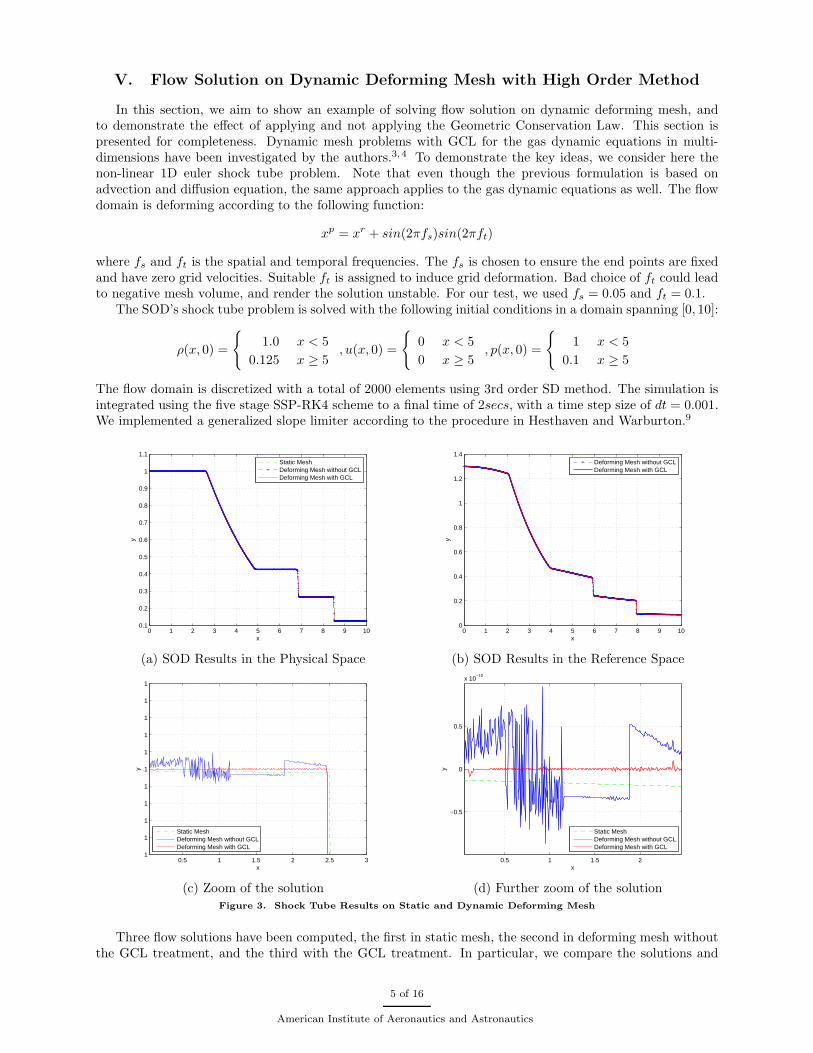
In this section, we aim to show an example of solving flow solution on dynamic deforming mesh, andto demonstrate the effect of applying and not applying the Geometric Conservation Law. This section ispresented for completeness. Dynamic mesh problems with GCL for the gas dynamic equations in multi-dimensions have been investigated by the authors.3, 4 To demonstrate the key ideas, we consider here thenon-linear 1D euler shock tube problem. Note that even though the previous formulation is based onadvection and diffusion equation, the same approach applies to the gas dynamic equations as well. The flowdomain is deforming according to the following function:

xp = xr + sin(2πfs)sin(2πft)

where fs and ft is the spatial and temporal frequencies. The fs is chosen to ensure the end points are fixedand have zero grid velocities. Suitable ft is assigned to induce grid deformation. Bad choice of ft could leadto negative mesh volume, and render the solution unstable. For our test, we used fs = 0.05 and ft = 0.1.

The SOD’s shock tube problem is solved with the following initial conditions in a domain spanning [0, 10]:

ρ(x, 0) =

{

1.0 x < 5

0.125 x ≥ 5, u(x, 0) =

{

0 x < 5

0 x ≥ 5, p(x, 0) =

{

1 x < 5

0.1 x ≥ 5

The flow domain is discretized with a total of 2000 elements using 3rd order SD method. The simulation isintegrated using the five stage SSP-RK4 scheme to a final time of 2secs, with a time step size of dt = 0.001.We implemented a generalized slope limiter according to the procedure in Hesthaven and Warburton.9

0 1 2 3 4 5 6 7 8 9 100.1

0.2

0.3

0.4

0.5

0.6

0.7

0.8

0.9

1

1.1

x

y

Static MeshDeforming Mesh without GCLDeforming Mesh with GCL

0 1 2 3 4 5 6 7 8 9 100

0.2

0.4

0.6

0.8

1

1.2

1.4

x

y

Deforming Mesh without GCLDeforming Mesh with GCL

(a) SOD Results in the Physical Space (b) SOD Results in the Reference Space

0.5 1 1.5 2 2.5 31

1

1

1

1

1

1

1

1

1

1

x

y


0.5 1 1.5 2

−0.5

0

0.5

x 10−10

x

y


(c) Zoom of the solution (d) Further zoom of the solutionFigure 3. Shock Tube Results on Static and Dynamic Deforming Mesh

Three flow solutions have been computed, the first in static mesh, the second in deforming mesh withoutthe GCL treatment, and the third with the GCL treatment. In particular, we compare the solutions and

5 of 16


examine the effect of the GCL. The solutions in the entire domain for the three cases are plotted togetherin figure 3(a)-(b). The moving shock flow solutions in the physical space are recovered in the deformingmesh in both cases. We also plot the flow solutions together in the reference space, showing the deformedsolutions. To more clearly examine the difference among the three cases, we zoom in the region spanning[0, 3] in figure 3(c)-(d). Here the effect of implementing the GCL is more clearly observed. In particular,the freestream error is significantly reduced when the GCL is enforced, compared to the larger and moreoscillatory error induced when the GCL is not formulated. The solution on deformed mesh with GCL alsoseems to be more accurate than the solution obtained using static mesh. This is likely due to the increasedmesh resolution due to mesh deformation. This is the topic that will be discussed in the rest of the paper.

VI. Dynamic Mesh Mapping for Mesh Resolution Enhancement

The mesh deformation can be used to efficiently distribute the mesh points so that regions where gradientsare high acquire more mesh points at the expense of low gradients regions. Hence if a mesh weighting functioncan be defined so that more weights are given to high gradient regions, we can achieve the desired distribution.Bercovici and Lele2 applied this idea to isotachophoresis analysis using compact finite difference scheme byformulating adaptive mesh deformation as an optimization problem. The optimization approach follows thework by,1 which is outlined next.

Adaptive Mesh Deformation as An Optimization Problem

Adaptive mesh deformation can be cast as an optimization problem, as in classical problems in the calculusof variations. The aim is to maximize the mesh points concentration at regions where the weights are high.Consider the following cost function

I(x) =

∫ b

a

w(ξ)Jdx =

∫ b

a

w(ξ)J2dξ =

∫ b

a

w(ξ)

(∂x

∂ξ

)2

dξ

where I is the cost function to be minimized, w(ξ) is the weighting function that depends on the flow solution(the flow gradient), J is the Jacobian of the deformation transformation (the mesh volume), a and b arethe left and right boundaries of the flow domain. When I is minimized for a given w, the mesh pointsdistribution are optimized through the Jacobian distribution. Now suppose δI can be written to first orderas

δI =

∫ b

a

Gδxdξ

where G is the gradient. Then by settingδx = −λG

an improvement is obtained for postive λ

δI = −λ

∫

G2dξ

The optimal is achieved when G = 0. The task remains to find the gradient G. If we consider an expansionof δI to first order, then

δI = I(x+δx)−I(x) =

∫ b

a

w(ξ)

(∂x

∂ξ+

∂(δx)

∂ξ

)2

dξ−

∫ b

a

w(ξ)

(∂x

∂ξ

)2

dξ =

∫ b

a

2w(ξ)∂x

∂ξ

∂(δx)

∂ξdξ+High Order Terms

where in the approximation, second order variations have been omitted. Now the first order variation canbe integrated by parts, and assuming fixed points such that δxa = 0 and δxb = 0, then

δI =

∫ b

a

2∂

∂ξ

(

w(ξ)∂x

∂ξ

)

δx dξ =

∫ b

a

2∂

∂ξ

(

w(ξ)J

)

δx dξ =

∫ b

a

G δx dξ

where the gradient is found to be G, expressed as follows

G = 2∂

∂ξ

(

w(ξ)J

)

6 of 16


Search Method with Steepest Descent

For this optimization problem, the design variable is x, which can be considered as the mesh point movements.For steepest descent, a simple mesh movement is taken in the negative gradient direction, towards to theoptimal grid position. The updated new position for a specific mesh point xi can now be written as

xn+1i = xn

i + δxi = xni − λGn

i

This can also be regarded as a forward integration in time with λ = ∆t such that

∂x

∂t= −G

This term provides both the position and the mesh velocity for the next time step, both of which are neededto solve the transformed equation in the computational domain.

Search Method with Smoothed Descent

The gradient for the current problem involves two derivatives with respect to ξ, hence smoothness of x isreduced by two order for each iteration. The smoothing can be introduced into the optimization processby replacing the gradient G by a smoothed gradient G, which is obtained through the following smoothingequation

G −∂

∂xǫ∂G

∂x= G

The improvement is now replaced by

δx = −λG, where λ = ∆t

The descent is still assured with any arbitrary large choice of ǫ.

Mesh Weight Function

Regions where more mesh points are required are the parts of flow domain where the flow solution has highgradients, positive or negative. Hence choosing the magnitude of the flow solution gradient as the meshweighting function, we obtain, after normalized by the maximum value, the following

w(ξ) =

∣∣∣∣∂u∂ξ

∣∣∣∣

(max

∣∣∣∣∂u∂ξ

∣∣∣∣)

+ const

where the const is added to prevent the weighting function from being set to zero when the solution becomesconstant. Since the normalized gradient is of order 1, a larger const value will render the weighting functionless sensitive, and vice versa.

VII. Adaptive Mesh Deformation for High Order Method

For the high order SD method, the standard computational domain is made up of a set of standard meshelements. Within each element, two sets of points are used. A set of interior solution points are used to storeflow solution. A second set of flux points are used to store flux. Solutions at the mesh element interfacesare extrapolated from the interior solutions. In the standard mesh element, the mesh points are essentiallyreferred to the interfaces of the mesh elements, not the interior flux or solution points. The Jacobian Ji

corresponds to the mesh volume at interface i while the mesh velocity Vi is the ith interface velocity. Hencethe procedure outlined below is carried out by looping over the element interfaces. The procedure of usingadaptive mesh deformation for mesh refinement with the high order method can be summarized as follows

• Starting with solution uc in the computation domain at the current time step t

• Compute the gradient of the solution ∂u∂ξ

7 of 16


• Compute the mesh weighting function w(ξ)

• Compute the mesh transformation Jacobian J = ∂x∂ξ

• Compute the gradient of descent or improvement G = 2 ∂∂ξ

(w(ξ)J)

• Smooth the gradient to get G

• Compute the mesh velocity V = G

• Compute the next mesh point position by advancing to the next time step xt+dt = xt + dt · G

• At the new time step t + dt, with the new mesh position, compute the new mapping Jacobian J = ∂x∂ξ

• Compute the flow solution in the computational domain using J and V

This procedure can then be repeated as time advances.To demonstrate the effect of the adaptation scheme, two examples are shown in the following sections.

The results are quantitative, serving to illustrate the adaptive deforming idea. More qualitative results willfollow.

Steady State Mesh Refinement Problem with Standard SD Mesh Elements

If the goal is to refine the mesh points, without having to solve the flow equation dynamically as the meshpoints are being moved, then the problem simplifies to a pure optimization problem. An example is providedin this section to demonstrate the application of optimization method for mesh refinement. Consider asteady state problem starting with an equal-spaced mesh. The goal is to achieve the mesh points distributionthat matches the steady state solution gradient. The flow solution we considered has an initial Gaussian

−1 −0.8 −0.6 −0.4 −0.2 0 0.2 0.4 0.6 0.8 1−0.5

0

0.5

1

1.5

x

y

SD Mesh Element Distribution at Time t=0.2

Adaptively Deformed Mesh ElementsOriginal Equal Spaced Mesh Elements

−1 −0.8 −0.6 −0.4 −0.2 0 0.2 0.4 0.6 0.8 1−0.5

0

0.5

1

1.5

x

y



(a) t=0.2s (b) t=0.4s

−1 −0.8 −0.6 −0.4 −0.2 0 0.2 0.4 0.6 0.8 1−0.5

0

0.5

1

1.5

x

y



−1 −0.8 −0.6 −0.4 −0.2 0 0.2 0.4 0.6 0.8 1−0.5

0

0.5

1

1.5

x

y



(c) t=0.6s (d) t=0.8sFigure 4. Adaptively Deformed Mesh Elements at Various Time Steps, with λ = 1 and const = 0.5. SD order=5. TotalElements=40.

8 of 16


distribution. As time progresses, it remains at its initial position as the mesh point distribution is optimizedthrough mesh deformation. The initial condition is

u = ex2

The flow domain covers [-1,1] with a total of 40 SD elements. Within each element, 5 solution points areused, corresponding to 5th order SD method. The five stage Runge-Kutta 4 scheme is used to integrate timeforward until T = 1s. The results are plotted in figure 4 (a)-(d). As time advances, the number of meshpoints near high gradient regions is effectively increased. The eventual grid distribution and the rate withwhich the mesh points adapt to the solution depend on the choice of λ and const. In this case, we havechosen λ = 1 and const = 0.5.

Dynamic Mesh Refinement Problem with Standard SD Mesh Elements

For dynamic problems, the flow solution evolves over time. The mesh point distribution should adapt to thechanging solution. Let’s consider a linear advection equation as follows

∂u

∂t+ a

∂u

∂x= 0, with a = 0.2

with the initial conditionu = ex2

The flow domain covers [-0.8,1.2] with a total of 40 SD elements. As before, 5th order SD method is used for

−0.8 −0.6 −0.4 −0.2 0 0.2 0.4 0.6 0.8 1 1.2−0.5

0

0.5

1

1.5

x

y



−0.8 −0.6 −0.4 −0.2 0 0.2 0.4 0.6 0.8 1 1.2−0.5

0

0.5

1

1.5

x

ySD Mesh Element Distribution at Time t=0.4


(a) t=0.2s (b) t=0.4s

−0.8 −0.6 −0.4 −0.2 0 0.2 0.4 0.6 0.8 1 1.2−0.5

0

0.5

1

1.5

x

y



−0.8 −0.6 −0.4 −0.2 0 0.2 0.4 0.6 0.8 1 1.2−0.5

0

0.5

1

1.5

x

y



(c) t=0.6s (d) t=0.8s

Figure 5. Adaptively Deformed Mesh Elements at Various Time Steps, with λ = 1 and const = 0.25. SD order=5. TotalElements=40.

space discretization and the five stage Runge-Kutta 4 scheme is used to integrate time forward until T = 1s.Adaptively deformed and refined mesh elements at various time steps, with λ = 1 and const = 0.25, areshown in figure 5 (a)-(d). Grid point refinements near high gradient regions are observed at each time step.

9 of 16


VIII. Simultaneous Flow Solution and Adaptive Mesh Deformation

So far, we have demonstrated in this study that, independently, we can solve flow equation on dynamicallydeforming mesh given the required mapping metrics, and optimize mesh distribution through mesh pointsdeformation by advancing forward in time. In this section, the two methods are integrated to advancethe adaptive mesh refinement concurrently with flow solution in a dynamic environment using high ordermethod. In the following, we apply the above method to a finite volume scheme. The adaptive formulationfor SD scheme requires further steps. This will be discussed in the subsequent sections.

Dynamic Mesh Refinement Results with Finite Volume Method

From the SD method, we can obtain a cell center type of finite volume scheme by placing one solutionpoint within each mesh cell. The application of the adaptive mesh deforming algorithm to the finite volumescheme is straightforward, since all the mesh interface velocities can be evaluated directly. We again solvethe advection equation on increasing finer meshes, first with the finite volume method on fixed mesh, andthen with adaptive mesh deformation. The two results are presented in figure 6 and figure 7. In the figures,the exact solution at the final time is represented by blue dashed line at the final time, and black dottedline at the initial position. The red solid line represents the computed solution. Green dash-dotted linerepresents the normalized value of the cell Jacobian. When mesh is not deformed, the cell Jacobian has unitvalue. The region with small cell Jacobians has finer meshes.

−20 −10 0 10 20 30 40 50 60 70 80−2

0

2

4

6

8

10

12

x

y

Initial Computed Exact Mesh Jacobian

−20 −10 0 10 20 30 40 50 60 70 80−2

0

2

4

6

8

10

12

x

y


−20 −10 0 10 20 30 40 50 60 70 80−2

0

2

4

6

8

10

12

x

y


(a) 80 elements (b) 160 elements (b) 320 elements

Figure 6. Convection equation solved using 1st order SD method with increasingly finer meshes, without refinement

−20 −10 0 10 20 30 40 50 60 70 80−2

0

2

4

6

8

10

12

x

y


−20 −10 0 10 20 30 40 50 60 70 80−2

0

2

4

6

8

10

12

x

y


−20 −10 0 10 20 30 40 50 60 70 80−2

0

2

4

6

8

10

12

x

y


(a) 80 elements (b) 160 elements (b) 320 elementsFigure 7. Convection equation solved using 1st order SD method with increasingly finer meshes, with R-refinement

For very coarse and very dissipative scheme such as the present one, the adaptive mesh deformationis very effective. In the above example, the adaptive method produces result on the 80 mesh elementsthat is comparable to the result obtained with the non-adaptive method on 640 mesh elements. The errorconvergences for the two methods are plotted in figure 8. From the figure it is easy to see that the adaptivemethod consistently produces less errors than the method on fixed meshes for the cases considered. It alsoconverges towards the expected order faster.

Note of the Choices of λ and ǫ

The choices of λ and ǫ in the adaptive algorithm play a rather important role in determining the rate andthe amount of adaptation, which in turn determine the accuracy of the final solution. At present, the values

10 of 16


are assigned through experiments. In general, larger ǫ leads to very smooth mesh adaptation, which inducesbetter stability. Larger λ leads to quicker rate of adaptation. If λ is chosen too aggressively, the stability willbe affected. On the other hand, for initial value problem on very coarse mesh with very dissipative scheme,it is very important to minimize numerical dissipation as early and as quickly as possible because subsequentrefinement can only minimize further dissipation, but cannot help to restore the errors in the earlier history.Therefore, judicious choice of λ and ǫ will lead to good adaptation results, and vice versa. Automation ofthis process will be very useful and need to be pursued further. In the current example, λ is in the proximityof 1,000, and ǫ of 500.

10−4

10−3

10−2

10−1

100

101

102

Mesh Element Size

L ∞ E

rror

With Adaptive MeshWithout Adaptive Mesh1st Order Convergence

Figure 8. Error comparison and convergence

Extension to High-order SD scheme with Staggered SD and Finite Volume Mesh

To solve the time-dependent flow solution on the dynamic mesh, mesh velocities are needed as we know fromthe earlier formulation of transformed equation. Unlike the finite volume scheme, high-order SD methodrequires mesh velocities at interior flux points are needed in order to solve the transformed equation. This isnot directly available since the method outlined above operates on mesh element interfaces only. One way toobtain the interior flux point velocities are through interpolation using the element interface velocities at twoends. But the accuracy might be compromised by this simple approach. An alternative approach is outlinedhere by considering a mapping of the SD scheme from the high order mesh element into an equivalent finitevolume mesh. Method to solve the SD scheme on an equivalent finite volume mesh that reflects all theoriginal degrees of freedom is discussed next.

(a) FV and SD Cells in 1D (b) FV and SD Cells in 2D

Figure 9. Comparison of equally spaced finite volume cells and non equally distributed SD solution/flux points in 1Dand 2D

To better reflect the true number of degrees of freedom in the high order method, consider augmentingthe original reference physical domain (the undeformed physical domain) mesh by dividing each SD meshelements into N equally spaced sub cells, where N is the number of solution points. Hence, this effectivelybecomes an equal spaced finite volume mesh with the number of finite volume cells equal to the number of

11 of 16


solution points. This is illustrated in figure 9. The finite volume vertices correspond to the flux points, whilethe finite volume cell centers correspond to the solution points. The mapping between the equally spacedfinite volume cell centers and the solution points locations, such as zeros of the Legendre polynomials, areprecomputed and stored, and similarly for the mapping between the equally spaced finite volume verticesand the flux points locations. To make this even simpler, since the solution point distribution does not affectthe stability of the scheme, the solution points can be chosen to be equally distributed so that the mappingfrom solution points to the cell centers is direct. This same cannot be done for the flux points due to stabilityconcern, as discussed earlier in the section on SD formulation.

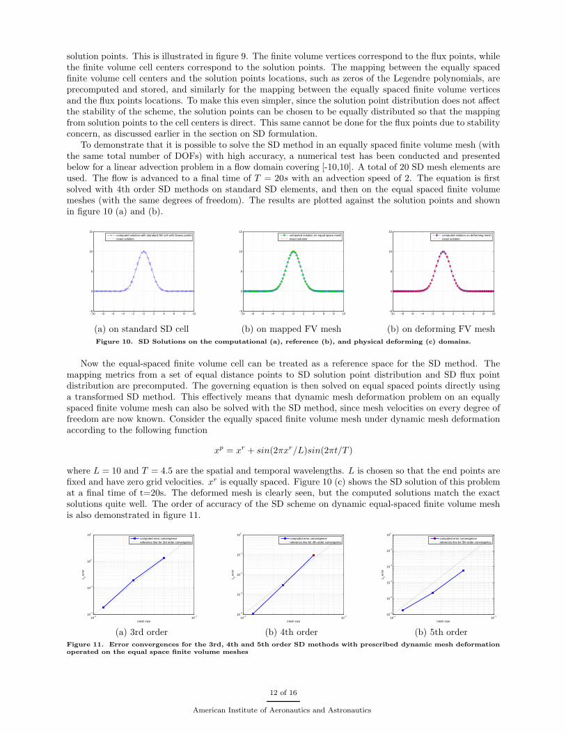
To demonstrate that it is possible to solve the SD method in an equally spaced finite volume mesh (withthe same total number of DOFs) with high accuracy, a numerical test has been conducted and presentedbelow for a linear advection problem in a flow domain covering [-10,10]. A total of 20 SD mesh elements areused. The flow is advanced to a final time of T = 20s with an advection speed of 2. The equation is firstsolved with 4th order SD methods on standard SD elements, and then on the equal spaced finite volumemeshes (with the same degrees of freedom). The results are plotted against the solution points and shownin figure 10 (a) and (b).

−10 −8 −6 −4 −2 0 2 4 6 8 10−5

0

5

10

15

computed solution with standard SD cell with Gauss pointsexact solution

−10 −8 −6 −4 −2 0 2 4 6 8 10−5

0

5

10

15

computed solution on equal space meshexact solution

−10 −8 −6 −4 −2 0 2 4 6 8 10−5

0

5

10

15

computed solution on deforming meshexact solution

(a) on standard SD cell (b) on mapped FV mesh (b) on deforming FV mesh

Figure 10. SD Solutions on the computational (a), reference (b), and physical deforming (c) domains.

Now the equal-spaced finite volume cell can be treated as a reference space for the SD method. Themapping metrics from a set of equal distance points to SD solution point distribution and SD flux pointdistribution are precomputed. The governing equation is then solved on equal spaced points directly usinga transformed SD method. This effectively means that dynamic mesh deformation problem on an equallyspaced finite volume mesh can also be solved with the SD method, since mesh velocities on every degree offreedom are now known. Consider the equally spaced finite volume mesh under dynamic mesh deformationaccording to the following function

xp = xr + sin(2πxr/L)sin(2πt/T )

where L = 10 and T = 4.5 are the spatial and temporal wavelengths. L is chosen so that the end points arefixed and have zero grid velocities. xr is equally spaced. Figure 10 (c) shows the SD solution of this problemat a final time of t=20s. The deformed mesh is clearly seen, but the computed solutions match the exactsolutions quite well. The order of accuracy of the SD scheme on dynamic equal-spaced finite volume meshis also demonstrated in figure 11.

10−2

10−1

10−2

10−1

100

101

mesh size

L 2 err

or

computed error convergencereference line for 3rd order convergence

10−2

10−1

10−4

10−3

10−2

10−1

100

mesh size

L 2 err

or

computed error convergencereference line for 4th order convergence

10−2

10−1

10−5

10−4

10−3

10−2

10−1

100

mesh size

L 2 err

or

computed error convergencereference line for 5th order convergence

(a) 3rd order (b) 4th order (b) 5th orderFigure 11. Error convergences for the 3rd, 4th and 5th order SD methods with prescribed dynamic mesh deformationoperated on the equal space finite volume meshes

12 of 16


The current proposed method has the finite volume solution space coincided with the reference SDsolution space, hence the solutions computed by either methods can be interchanged freely. The previouslyoutlined mesh optimization procedure can be now operated on the finite volume mesh and solved in the SDcomputational space. The results are presented in the following section.

IX. SD Results of Adaptive R-refinement with Dynamic Deforming Mesh

We have considered the 2nd, 3rd and 4th order solutions for the adaptive SD methods on very coarsemeshes to illustrate the benefits of the current method. High order methods on fine meshes have littledissipation in the first place so mesh adaptation might not be as necessary. The second order results areshown in figure 12. Figure 12 (a), (b) and (c) are results without mesh adaptation, while figure 12 (e),(f) and (g) are results without mesh adaptation. Similar results for the 3rd and 4th order solutions arepresented in figure 13 and figure 14. From those figures, we see that for those cases we considered here hemesh adaptation method works quite well for the SD method on very coarse mesh. On those very coarsemeshes considered here, the high-order schemes do not converge spectrally according to the expected orderof accuracy (until mesh is further refined). The L∞ and L2 error convergences for the 2nd, 3rd and 4thorder method are shown in figure 15. The blue line with circle marker shows the error convergences withoutadaptation. The red line with square marker shows the error convergences with adaptation. The accuraciesof the scheme have been improved with the adaptive mesh deformation. The choices of λ and ǫ for theresults are: λ = 800 and ǫ = 400 for the 2nd order, λ = 800 and ǫ = 200 for the 3rd order, and λ = 800 andǫ = 50 for the 4th order. Finally figure 16 illustrates more clearly the effect of the adaptation for the highorder solution by plotting the meshes with the result near the solution, which in this example is obtainedwith the 3rd order SD method on 40 mesh elements.

−20 −10 0 10 20 30 40 50 60 70 80−2

0

2

4

6

8

10

12

x

y


−20 −10 0 10 20 30 40 50 60 70 80−2

0

2

4

6

8

10

12

x

y


−20 −10 0 10 20 30 40 50 60 70 80−2

0

2

4

6

8

10

12

x

y


(a) 20 elements (b) 40 elements (d) 80 elements

−20 −10 0 10 20 30 40 50 60 70 80−2

0

2

4

6

8

10

12

x

y


−20 −10 0 10 20 30 40 50 60 70 80−2

0

2

4

6

8

10

12

x

y


−20 −10 0 10 20 30 40 50 60 70 80−2

0

2

4

6

8

10

12

x

y


(e) 20 elements (f) 40 elements (g) 80 elements

Figure 12. Convection equation solved using 2nd order SD method with increasingly finer meshes with (bottom row)and without refinement (top row)

X. Conclusion

In this paper we have formulated and implemented two frameworks. In the first, we are able to solvehigh order SD method on dynamic deforming mesh given the mesh deformation function. In the second,the mesh refinement through adaptive mesh deformation has been regarded as an optimization problem andadaptive refinement has been demonstrated for both steady state and time dependent solution. These twoframeworks have been integrated for the high-order SD method so that we can advance the solution on thenew mesh at the same time as the mesh is being refined. More specifically, we have proposed here to solve

13 of 16


−20 −10 0 10 20 30 40 50 60 70 80−2

0

2

4

6

8

10

12

x

y


−20 −10 0 10 20 30 40 50 60 70 80−2

0

2

4

6

8

10

12

x

y


−20 −10 0 10 20 30 40 50 60 70 80−2

0

2

4

6

8

10

12

x

y



−20 −10 0 10 20 30 40 50 60 70 80−2

0

2

4

6

8

10

12

x

y


−20 −10 0 10 20 30 40 50 60 70 80−2

0

2

4

6

8

10

12

x

y


−20 −10 0 10 20 30 40 50 60 70 80−2

0

2

4

6

8

10

12

x

y



Figure 13. Convection equation solved using 3rd order SD method with increasingly finer meshes with (bottom row)and without refinement (top row)

−20 −10 0 10 20 30 40 50 60 70 80−2

0

2

4

6

8

10

12

x

y


−20 −10 0 10 20 30 40 50 60 70 80−2

0

2

4

6

8

10

12

x

y


−20 −10 0 10 20 30 40 50 60 70 80−2

0

2

4

6

8

10

12

x

y



−20 −10 0 10 20 30 40 50 60 70 80−2

0

2

4

6

8

10

12

x

y


−20 −10 0 10 20 30 40 50 60 70 80−2

0

2

4

6

8

10

12

x

y


−20 −10 0 10 20 30 40 50 60 70 80−2

0

2

4

6

8

10

12

x

y



Figure 14. Convection equation solved using 4th order SD method with increasingly finer meshes with (bottom row)and without refinement (top row)

the SD method accurately on an equivalent equal spaced finite volume mesh, which has the same number ofdegree of freedoms as the actual SD method. With this proposed method, the physical moving domain is nowpopulated with the same mesh points as the true degrees of freedoms, hence both J , the mapping Jacobians,and V , the mesh point velocities, can be more accurate represented. In addition, each solution and fluxpoint have their corresponding mesh points in the physical space, hence the associated mesh velocities arenow also readily available without the need for inaccurate interpolation. In summary, the current studypresents an effort to develop a flexible (through domain transformation), efficient (through mesh refinement)and accurate (through the staggered finite volume mesh) high order method.

14 of 16


10−3

10−2

10−1

10−2

10−1

100

101

102

Mesh Element Size

L ∞ E

rror

With Adaptive MeshWithout Adaptive Mesh2nd Order Convergence

10−3

10−2

10−1

10−3

10−2

10−1

100

101

102

103

Mesh Element Size

L ∞ E

rror

With Adaptive MeshWithout Adaptive Mesh3rd Order Convergence

10−2

10−1

10−2

10−1

100

101

102

Mesh Element Size

L ∞ E

rror

With Adaptive MeshWithout Adaptive Mesh4th Order Convergence

10−3

10−2

10−1

10−2

10−1

100

101

102

Mesh Element Size

L 2 Err

or

With Adaptive MeshWithout Adaptive Mesh2nd Order Convergence

10−3

10−2

10−1

10−3

10−2

10−1

100

101

102

103

Mesh Element Size

L 2 Err

or

With Adaptive MeshWithout Adaptive Mesh3rd Order Convergence

10−2

10−1

10−2

10−1

100

101

102

Mesh Element Size

L 2 Err

or

With Adaptive MeshWithout Adaptive Mesh4th Order Convergence

(a) 2nd order (b) 3rd order (c) 4th orderFigure 15. Comparison of the error convergences for the 2nd, 3rd and 4th order SD method with and without adaptivemesh deformation. Top row is based on L∞ norm. Bottom row is based on L2 norm.

50 52 54 56 58 60 62 64 66 68 70−5

0

5

10

15

x

y

SD SolutoinSolution PointCell BoundaryExact SolutionSolution PointCell BoundaryError

50 52 54 56 58 60 62 64 66 68 70−5

0

5

10

15

x

y

SD SolutoinSolution PointCell BoundaryExact SolutionSolution PointCell BoundaryError

(a) solution and SD mesh cells without adaptation (b) solution and SD mesh cells with adaptationFigure 16. Zoom of the final solution. The SD mesh cells are plotted together with the solution points within theelements. Note that the solutions are plotted at the flux points, not the solution points

Acknowledgement

This research work is made possible by the generous fundings from the National Science Foundation andthe Air Force Office of Scientific Research under the grants 0708071 and 0915006 monitored by Dr. LelandJameson, and grant FA9550-07-1-095 by Dr. Fariba Fahroo. The authors would like to thank them for theircontinuous support.

References

1A. Jameson and J. Vassberg, “Studies of Alternative Numerical Optimization Methods Applied to the BrachistochroneProblem”, OptiCon 99 Conference, Newport Beach, CA, October 1999, Computational Fluid Dynamics Journal, Vol. 9, 2000,pp. 281-296.

2M. Bercovici and S.K. Lele, “Compact adaptive-grid scheme for high numerical resolution simulation of isotachophoresis”,Journal of Chromatography A, vol. 1217, 2010, pp.588-599.

3K. Ou, C. Liang, A. Jameson, “High-Order Spectral Difference Method for the Navier-Stokes Equations on UnstructuredMoving Deformable Grids”, AIAA-2010-541, 48th AIAAAerospace Sciences Meeting, Orlando, Jan 2010.

4K. Ou and A. Jameson, “On the Temporal and Spatial Accuracy of Spectral Difference Method on Moving DeformableGrids and the Effect of Geometric Conservation Law”, AIAA-2010-5032, 40th Fluid Dynamics Conference and Exhibit, Chicago,Illinois, June 28-1, 2010

15 of 16


5Huynh, H.T., “A flux reconstruction approach to high-order schemes including discontinuous Galerkin methods”, AIAA2007-4079,18th AIAA CFD Conference, Miami, June 2008.

6Liu,Y., Vinokur, M., Wang, Z.J., “Spectral difference method for unstructured grids I: Basic formulation”, J. Comput.Phy., 216, 2006, 780-801.

7Z.J. Wang, Y. Liu, G. May and A. Jameson, “Spectral Difference Method for Unstructured Grids II: Extension to theEuler Equations, Journal of Scientific Computing, Vol. 32, No. 1, pp. 45-71 (2007).

8Y. Sun and Z. J. Wang and Y. Liu, “High-order multidomain spectral difference method for the Navier-Stokes equationson unstructured hexahedral grids, Communication in Computational Physics, Vol. 2, pp. 310-333 (2007).

9J. S. Hesthaven and T. Warburton, Nodal discontinuous Galerkin methods - Algorithms, analysis, and applications,Springer, (2008).

16 of 16


dynamic mesh deformation for adaptive grid resolution...

Documents