dynamic modeling of cerebral blood ... - rc.library.uta.edu
TRANSCRIPT

DYNAMIC MODELING OF CEREBRAL BLOOD
FLOW AUTOREGULATION USING ARX
AND WINDKESSEL MODELS
PIYUSH GEHALOT
Presented to the Faculty of the Graduate School of
The University of Texas at Arlington in Partial Fulfillment
of the Requirements
for the Degree of
MASTER OF SCIENCE IN BIOMEDICAL ENGINEERING
THE UNIVERSITY OF TEXAS AT ARLINGTON
August 2005

Copyright © by Piyush Gehalot 2005
All Rights Reserved

DEDICATED TO MY FAMILY

iv
ACKNOWLEDGEMENTS
I would like to express my sincere gratitude to Dr. Khosrow Behbehani,
Professor and Chair, Department of Bioengineering at UTA, for providing me with the
opportunity to work and for providing constant encouragement and timely guidance
throughout this study.
I would also like to thank Dr. Rong Zhang, Assistant Professor, Internal
Medicine – Cardiology Division, University of Texas Southwestern Medical Center at
Dallas and Dr. Hanli Liu, Assistant Professor, Department of Bioengineering at UTA
for helping me meet all the deadlines and providing valuable suggestions.
A special thanks to the volunteers who participated in this study. This study
would not have been possible without their time and interest.
I would also like to thank Aby Mathew and my co-workers at the lab - Ganesh
and Suhas for their kind co-operation. All the help and co-operation of faculty and staff
of the Department of Bioengineering is also greatly appreciated.
And finally, I would like to thank my family in India for supporting me in every
possible means. This would not have been possible without their and God’s blessings.
July 25, 2005
v
ABSTRACT
DYNAMIC MODELING OF CEREBRAL BLOOD
FLOW AUTOREGULATION USING ARX
AND WINDKESSEL MODELS
Publication No. ______
Piyush Gehalot, M. S.
The University of Texas at Arlington, 2005
Supervising Professor: Khosrow Behbehani, Ph.D., P.E.
Linear lumped parameter models like ARX and Windkessel models are simple,
easy to solve, and find their application in real time modeling. The present study is
focused on employing single input single output ARX and Windkessel models to beat-
to-beat mean arterial blood pressure (MABP, mmHg) considered as input to the model,
and cerebral blood flow velocity (CBFV, cm/sec) considered as output of the model.
For some models and modeling methodologies, the data consisted of cerebral perfusion
pressure (CPP, mmHg, estimated from MABP) and CBFV. The data was measured
from 10 healthy normal subjects while the subjects performed Valsalva maneuver with
and without the ganglion blockade by the use of trimethaphan. The main objective of

vi
this study was to examine the relative performance and limitations of the above
mentioned linear modeling options and to demonstrate newer modeling methodologies
for them. Also, since for linear model estimation it is required that the input be
persistently exciting, the present study aimed to establish the efficacy of MABP for
estimation of linear models and tested if a short data segment of 1.5 minute duration is
adequate for the same, as compared to the traditional 6 minutes data.
Two ARX modeling schemes investigating up to 10th order models, and three
schemes for Windkessel modeling involving the 3-element model and four of its
modified versions of 4 or 5 elements, were employed in the present study. Even though
the study was not restricted to lower order systems or simple Windkessel models,
results indicate that lower order ARX models (1st, 2nd, and 3rd order ARX models) and
the 3-element Windkessel model are adequate. Among the ARX and Windkessel
methodologies, ARX modeling schemes proved more promising. The results of using
CPP-CBFV data were not better than the results of using MABP-CBFV data.
It is clear that the models used for the present study had very basic mechanisms
and structures, but were still able to reproduce the measured data. Also, tests involving
the 1.5 minute MABP using the ARX models and results from the Monte-Carlo
simulations of Windkessel models using two schemes suggest that a segment of 1.5
minute duration of MABP is effective and adequate for estimating linear models of
cerebral autoregulation.

vii
TABLE OF CONTENTS
ACKNOWLEDGEMENTS………………………………………………………... iv ABSTRACT………………………………………………………………………... v LIST OF ILLUSTRATIONS………………………………………………………. ix LIST OF TABLES…………………………………………………………………. xix LIST OF ABBREVIATIONS ……………………………………………………... xxiv Chapter 1. INTRODUCTION…………………………………………………………. 1 1.1 Cerebral Autoregulation…………………………………………….. 1 1.2 Valsalva Maneuver……………………………………………….…. 3
1.3 Previous Studies Involving Human Cerebral Circulation and Its Modeling……………………....................................................... 6
1.4 Objectives and Overview of the Thesis………………………… ...... 7 2. METHODS………………………………………………………………… 11 2.1 Experimental Setup and Data Acquisition………………………….. 11 2.2 Modeling Methodologies……………………………………………. 16 2.3 Establishing the Adequacy and Efficacy of 1.5 Minute MABP as Input Stimulus…………………………………………………….... 39 2.4 Estimating Cerebral Perfusion Pressure from MABP…………….. .. 45
3. RESULTS………………………………………………………………….. 48 3.1 Results for Establishing the Adequacy and Efficacy of 1.5 Minute MABP as Input Stimulus ………………………………. 48

viii
3.2 Modeling Results for MABP and CBFV Data…… ........................... 82 3.3 Modeling Results for CPP and CBFV Data ……………………....... 130 4. DISCUSSION AND LIMITATIONS…………………………………….. . 133 4.1 Discussion for the Results of Testing the Adequacy and Efficacy of 1.5 Minute MABP as Input Stimulus………………….. 133 4.2 Discussion of the Modeling Results for MABP and CBFV Data....... 137 4.3 Discussion of the Modeling Results for CPP and CBFV Data..... ...... 144 4.4 Limitations………………………………………………………….. 145 5. CONCLUSIONS AND DIRECTIONS FOR FUTURE WORK. ................. 146 5.1 Conclusions…………………………………………………………. 146 5.2 Directions for Future Work…………………………………………. 148 Appendix A. DATA ANALYSIS ALGORITHMS AND PROGRAMS ........................... 149 B. COMPARISON OF MSE AND PARAMETER VALUES .......................... 160 REFERENCES…………………………………………………………………….. 171 BIOGRAPHICAL INFORMATION………………………………………………. 178

ix
LIST OF ILLUSTRATIONS
Figure Page 1.1 Valsalva maneuver………………………………………………... ............... ….4 1.2 Phases (I through IV) associated with Valsalva maneuver…………………... …5 2.1 Spontaneous with no infusion (SNI) mean arterial blood pressure (MABP) and cerebral blood flow velocity (CBFV) data ……………………...14 2.2 Spontaneous with infusion (SI) mean arterial blood pressure (MABP) and cerebral blood flow velocity (CBFV) data ……………………...15 2.3 Valsalva maneuver with no infusion (VNI) mean arterial blood pressure
(MABP) and cerebral blood flow velocity (CBFV) data................................. ...15 2.4 Valsalva maneuver with infusion (VI) mean arterial blood pressure (MABP) and cerebral blood flow velocity (CBFV) data ….…… .................. ...16 2.5 ARX-1 modeling scheme ….…….................................................................. ...19 2.6 ARX-2 modeling scheme ….…….................................................................. ...20 2.7 Frank’s simple Windkessel model of arterial vascular system ….…… ......... ...21 2.8 Original (two-element) Windkessel model with one
resistor (R1) and one capacitor (C1) ……………………………………………22 2.9 Three-element Windkessel model with two resistors (R1 and R2) and one capacitor (C1).................................................... ...22 2.11 Windkessel 3-element model ….…… ............................................................ ...24 2.12 Modified Windkessel 5-element model ….…… ............................................ ...25 2.13 Modified Windkessel 5-element model ….…… ............................................ ...26 2.14 Modified Windkessel 5-element model ….…… ............................................ ...27

x
2.15 Modified Windkessel 4-element model ….…… ............................................ ...28 2.16 Windkessel-1 modeling scheme ….……........................................................ ...35 2.17 Windkessel-2 modeling scheme ….……........................................................ ...37 2.18 Windkessel-3 modeling scheme ….……........................................................ ...39 2.19 Steps 1 to 3 for the ARX modeling methodology for establishing the adequacy and efficacy of 1.5 minute MABP as input stimulus ….……... ...42 2.20 Step 4 for the ARX modeling methodology for establishing the adequacy and efficacy of 1.5 minute MABP as input stimulus….…….......... ...43
2.21 Methodology for Monte-Carlo simulations of Windkessel modeling schemes, for establishing the adequacy and efficacy of 1.5 minute MABP as input stimulus ….…… ................................................. ...44 2.22 Valsalva maneuver with no infusion (VNI) mean arterial blood pressure
(MABP) and cerebral perfusion pressure (CPP) data ….……........................ ...47 3.1 Histogram of true-parameter value for resistance parameter R1 of model 1 for Windkessel-1 modeling scheme with PRBS as the input…….................................................................................... ...51 3.2 Histogram of estimated -parameter value for resistance parameter R1 of model 1 for Windkessel-1 modeling scheme with PRBS as the input …. ...................................................................................... ...52 3.3 Histogram of true-parameter value for resistance parameter R1 of model 2 for Windkessel-1 modeling scheme with PRBS as the input ….…….............................................................................. ...53 3.4 Histogram of estimated -parameter value for resistance parameter R1 of model 2 for Windkessel-1 modeling scheme with PRBS as the input …. ...................................................................................... ...53 3.5 Histogram of true-parameter value for resistance parameter R1 of model 3 for Windkessel-1 modeling scheme with PRBS as the input ….…….............................................................................. ...54 3.6 Histogram of estimated -parameter value for resistance parameter R1 of model 3 for Windkessel-1 modeling scheme with PRBS as the input ….… .................................................................................. ...55
xi
3.7 Histogram of true-parameter value for resistance parameter R1 of model 4 for Windkessel-1 modeling scheme with PRBS as the input ….…….............................................................................. ...56 3.8 Histogram of estimated -parameter value for resistance parameter R1 of model 4 for Windkessel-1 modeling scheme with PRBS as the input ….….................................................................................. ...56 3.9 Histogram of true-parameter value for resistance parameter R1 of model 5 for Windkessel-1 modeling scheme with PRBS as the input ….…….............................................................................. ...57 3.10 Histogram of estimated -parameter value for resistance parameter R1 of model 5 for Windkessel-1 modeling scheme with PRBS as the input …. ...................................................................................... ...58 3.11 Histogram of true-parameter value for resistance parameter
R1 of model 1 for Windkessel-1 modeling scheme with MABP as the input……………………………………………………………..59
3.12 Histogram of estimated -parameter value for resistance parameter R1 of model 1 for Windkessel-1 modeling scheme with MABP as the input …...................................................................................... ...60
3.13 Histogram of true-parameter value for resistance parameter R1 of model 2 for Windkessel-1 modeling scheme with MABP as the input …...................................................................................... ...61
3.14 Histogram of estimated -parameter value for resistance parameter R1 of model 2 for Windkessel-1 modeling scheme with MABP as the input …...................................................................................... ...61
3.15 Histogram of true-parameter value for resistance parameter R1 of model 3 for Windkessel-1 modeling scheme with MABP as the input …...................................................................................... ...62
3.16 Histogram of estimated -parameter value for resistance parameter R1 of model 3 for Windkessel-1 modeling scheme with MABP as the input …...................................................................................... ...63
3.17 Histogram of true-parameter value for resistance parameter R1 of model 4 for Windkessel-1 modeling scheme with MABP as the input …...................................................................................... ...64

xii
3.18 Histogram of estimated -parameter value for resistance parameter R1 of model 4 for Windkessel-1 modeling scheme with MABP as the input …...................................................................................... ...64
3.19 Histogram of true-parameter value for resistance parameter R1 of model 5 for Windkessel-1 modeling scheme with MABP as the input…....................................................................................... ...65
3.20 Histogram of estimated -parameter value for resistance parameter R1 of model 5 for Windkessel-1 modeling scheme with MABP as the input …...................................................................................... ...66
3.21 Histogram of true-parameter value for resistance parameter R1 of model 1 for Windkessel-2 modeling scheme with PRBS as the input …. ...................................................................................... ...67 3.22 Histogram of estimated -parameter value for resistance parameter R1 of model 1 for Windkessel-2 modeling scheme with PRBS as the input …. ...................................................................................... ...68
3.23 Histogram of true-parameter value for resistance parameter R1 of model 2 for Windkessel-2 modeling scheme with PRBS as the input …. ...................................................................................... ...69 3.24 Histogram of estimated -parameter value for resistance parameter R1 of model 2 for Windkessel-2 modeling scheme with PRBS as the input …. ...................................................................................... ...69
3.25 Histogram of true-parameter value for resistance parameter R1 of model 3 for Windkessel-2 modeling scheme with PRBS as the input …. ...................................................................................... ...70
3.26 Histogram of estimated -parameter value for resistance parameter R1 of model 3 for Windkessel-2 modeling scheme with PRBS as the input …. ...................................................................................... ...71
3.27 Histogram of true-parameter value for resistance parameter R1 of model 4 for Windkessel-2 modeling scheme with PRBS as the input…. ....................................................................................... ...72
3.28 Histogram of estimated -parameter value for resistance parameter R1 of model 4 for Windkessel-2 modeling scheme with PRBS as the input …. ...................................................................................... ...72

xiii
3.29 Histogram of true-parameter value for resistance parameter R1 of model 5 for Windkessel-2 modeling scheme with PRBS as the input …. ...................................................................................... ...73
3.30 Histogram of estimated -parameter value for resistance parameter R1 of model 5 for Windkessel-2 modeling scheme with PRBS as the input …. ...................................................................................... ...74
3.31 Histogram of true-parameter value for resistance parameter R1 of model 1 for Windkessel-2 modeling scheme with MABP as the input …...................................................................................... ...75 3.32 Histogram of estimated -parameter value for resistance parameter R1 of model 1 for Windkessel-2 modeling scheme with MABP as the input …...................................................................................... ...76
3.33 Histogram of true-parameter value for resistance parameter R1 of model 2 for Windkessel-2 modeling scheme with MABP as the input …...................................................................................... ...77
3.34 Histogram of estimated -parameter value for resistance parameter R1 of model 2 for Windkessel-2 modeling scheme with MABP as the input …...................................................................................... ...77
3.35 Histogram of true-parameter value for resistance parameter R1 of model 3 for Windkessel-2 modeling scheme with MABP as the input …...................................................................................... ...78 3.36 Histogram of estimated -parameter value for resistance parameter R1 of model 3 for Windkessel-2 modeling scheme with MABP as the input …...................................................................................... ...79
3.37 Histogram of true-parameter value for resistance parameter
R1 of model 4 for Windkessel-2 modeling scheme with MABP as the input………………......................................................................80
3.38 Histogram of estimated -parameter value for resistance parameter R1 of model 4 for Windkessel-2 modeling scheme with MABP as the input …...................................................................................... ...80
3.39 Histogram of true-parameter value for resistance parameter R1 of model 5 for Windkessel-2 modeling scheme with MABP as the input …...................................................................................... ...81

xiv
3.40 Histogram of estimated-parameter value for resistance parameter R1 of model 5 for Windkessel-2 modeling scheme with MABP as the input …...................................................................................... ...82
3.41 Plot of the outputs for model 1 with Windkessel-1 and Windkessel-2 modeling schemes for SNI data of subject no. 9 …. ....................................... .102
3.42 Plot of the frequency responses for model 1 with Windkessel-1 and Windkessel-2 modeling schemes for SNI data of subject no. 9 …. ................ .102
3.43 Plot of the model outputs with ARX-1 and ARX-2 (1st order model) modeling schemes for SNI data of subject no. 9 …. ....................................... .103
3.44 Plot of the model frequency responses with ARX-1 and ARX-2 (1st order model) modeling schemes for SNI data of subject no. 9 …. ........... .103
3.45 Plot of the outputs for model 2 with Windkessel-1 and Windkessel-2 modeling schemes for VI data of subject no. 3 …. ......................................... .104
3.46 Plot of the frequency responses for model 2 with Windkessel-1 and Windkessel-2 modeling schemes for VI data of subject no. 3 …. .................. .104
3.47 Plot of the model outputs with ARX-1 and ARX-2 (2nd order model) modeling schemes for VI data of subject no. 3 …. ......................................... .105
3.48 Plot of the model frequency responses with ARX-1 and ARX-2 (2nd order model) modeling schemes for VI data of subject no. 3 ….............. .105
3.49 Plot of the outputs for model 3 with Windkessel-1 and Windkessel-2 modeling schemes for VNI data of subject no. 1 …........................................ .106
3.50 Plot of the frequency responses for model 3 with Windkessel-1 and Windkessel-2 modeling schemes for VNI data of subject no. 1 …................. .106
3.51 Plot of the model outputs with ARX-1 and ARX-2 (3rd order model) modeling schemes for VNI data of subject no. 1 …........................................ .107
3.52 Plot of the model frequency responses with ARX-1 and ARX-2 (3rd order model) modeling schemes for VNI data of subject no. 1 …. .......... .107
3.53 Plot of the outputs for model 4 with Windkessel-1 and Windkessel-2 modeling schemes for SNI data of subject no. 9 …. ....................................... .108

xv
3.54 Plot of the frequency responses for model 4 with Windkessel-1 and Windkessel-2 modeling schemes for SNI data of subject no. 9 …. ................ .108
3.55 Plot of the model outputs with ARX-1 and ARX-2 (3rd order model) modeling schemes for SNI data of subject no. 9 …. ....................................... .109
3.56 Plot of the model frequency responses with ARX-1 and ARX-2 (3rd order model) modeling schemes for SNI data of subject no. 9 …............ .109
3.57 Plot of the outputs for model 4 with Windkessel-1 and Windkessel-2 modeling schemes for VI data of subject no. 3…. .......................................... .110 3.58 Plot of the frequency responses for model 4 with Windkessel-1 and Windkessel-2 modeling schemes for VI data of subject no. 3 …. .................. .110
3.59 Plot of the model outputs with ARX-1 and ARX-2 (3rd order model) modeling schemes for VI data of subject no. 3 …. ......................................... .111 3.60 Plot of the model frequency responses with ARX-1 and ARX-2
(3rd order model) modeling schemes for VI data of subject no. 3…………….111
3.61 Plot of the outputs for model 5 with Windkessel-1 and Windkessel-2 modeling schemes for VI data of subject no. 3 …. ......................................... .112
3.62 Plot of the frequency responses for model 5 with Windkessel-1 and Windkessel-2 modeling schemes for VI data of subject no. 3 …. .................. .112
3.63 Plot of the model outputs with ARX-1 and ARX-2 (2nd order model) modeling schemes for VI data of subject no. 3 …. ......................................... .113 3.64 Plot of the model frequency responses with ARX-1 and ARX-2 (2nd order model) modeling schemes for VI data of subject no. 3 ….............. .113
3.65 Plot of the outputs for model 1 with Windkessel-1 and Windkessel-2 modeling schemes for VI data of subject no. 2 …. ......................................... .114
3.66 Plot of the frequency responses for model 1 with Windkessel-1 and Windkessel-2 modeling schemes for VI data of subject no. 2 …. .................. .114
3.67 Plot of the model outputs with ARX-1 and ARX-2 (1st order model) modeling schemes for VI data of subject no. 2 …. ......................................... .115
3.68 Plot of the model frequency responses with ARX-1 and ARX-2 (1st order model) modeling schemes for VI data of subject no. 2 …............... 115

xvi
3.69 Plot of the outputs for model 2 with Windkessel-1 and Windkessel-2 modeling schemes for SNI data of subject no. 5 …. ....................................... .116
3.70 Plot of the frequency responses for model 2 with Windkessel-1 and Windkessel-2 modeling schemes for SNI data of subject no. 5 …. ................ .116
3.71 Plot of the model outputs with ARX-1 and ARX-2 (2nd order model) modeling schemes for SNI data of subject no. 5 …. ....................................... .117
3.72 Plot of the model frequency responses with ARX-1 and ARX-2 (2nd order model) modeling schemes for SNI data of subject no. 5 …. .......... .117
3.73 Plot of the outputs for model 3 with Windkessel-1 and Windkessel-2 modeling schemes for VNI data of subject no. 6 …........................................ .118
3.74 Plot of the frequency responses for model 3 with Windkessel-1 and Windkessel-2 modeling schemes for VNI data of subject no. 6 …................. .118
3.75 Plot of the model outputs with ARX-1 and ARX-2 (3rd order model) modeling schemes for VNI data of subject no. 6 …........................................ .119
3.76 Plot of the model frequency responses with ARX-1 and ARX-2 (3rd order model) modeling schemes for VNI data of subject no. 6 …. .......... .119
3.77 Plot of the outputs for model 4 with Windkessel-1 and Windkessel-2 modeling schemes for SNI data of subject no. 5…. ........................................ .120 3.78 Plot of the frequency responses for model 4 with Windkessel-1 and Windkessel-2 modeling schemes for SNI data of subject no. 5 …. ................ .120
3.79 Plot of the model outputs with ARX-1 and ARX-2 (3rd order model) modeling schemes for SNI data of subject no. 5 …. ....................................... .121
3.80 Plot of the model frequency responses with ARX-1 and ARX-2 (3rd order model) modeling schemes for SNI data of subject no. 5…............. .121
3.81 Plot of the outputs for model 4 with Windkessel-1 and Windkessel-2 modeling schemes for VI data of subject no. 2 …. ......................................... .122
3.82 Plot of the frequency responses for model 4 with Windkessel-1 and Windkessel-2 modeling schemes for VI data of subject no. 2 …. .................. .122
xvii
3.83 Plot of the model outputs with ARX-1 and ARX-2 (3rd order model) modeling schemes for VI data of subject no. 2 …. ......................................... .123
3.84 Plot of the model frequency responses with ARX-1 and ARX-2 (3rd order model) modeling schemes for VI data of subject no. 2 …. ............. .123
3.85 Plot of the outputs for model 5 with Windkessel-1 and Windkessel-2 modeling schemes for VNI data of subject no. 6 …........................................ .124
3.86 Plot of the frequency responses for model 5 with Windkessel-1 and Windkessel-2 modeling schemes for VNI data of subject no. 6 …................. .124
3.87 Plot of the model outputs with ARX-1 and ARX-2 (2nd order model) modeling schemes for VNI data of subject no. 6 …........................................ .125
3.88 Plot of the model frequency responses with ARX-1 and ARX-2
(2nd order model) modeling schemes for VNI data of subject no. 6 ………….125
3.89 Plot of the outputs for model 5 with Windkessel-1 and Windkessel-2 modeling schemes for VI data of subject no. 2 …. ......................................... .126
3.90 Plot of the frequency responses for model 5 with Windkessel-1 and Windkessel-2 modeling schemes for VI data of subject no. 2 …. .................. .126
3.91 Plot of the model outputs with ARX-1 and ARX-2 (2nd order model) modeling schemes for VI data of subject no. 2 …. ......................................... .127
3.92 Plot of the model frequency responses with ARX-1 and ARX-2 (2nd order model) modeling schemes for VI data of subject no. 2 ….............. .127
3.93 Plot of the output for model 1 with Windkessel-3 modeling scheme for SNI data of subject no. 9 …....................................................................... .128
3.94 Plot of the frequency response for model 1 with Windkessel-3 modeling scheme for SNI data of subject no. 9 ….......................................... .128
3.95 Plot of the output for model 1 with Windkessel-3 modeling scheme for VI data of subject no. 2 …. ........................................................................ .129
3.96 Plot of the frequency response for model 1 with Windkessel-3 modeling scheme for VI data of subject no. 2 …. ........................................... .129
3.97 Plot of the output for model 1 with Windkessel-1 modeling scheme for CPP-CBFV VI data of subject no. 2 …. .................................................... .131

xviii
3.98 Plot of the frequency response for model 1 with Windkessel-1 modeling scheme for CPP-CBFV VI data of subject no. 2…. ........................ .132
xix
LIST OF TABLES
Table Page 3.1 MSE values of 10 subjects for Ma, Me1 and Me2…......................................... ...49 3.2 Comparison (t-test) of MSE values between 6 minute and 1.5 minute data sets of 10 subjects …. ............................................................ ...50 3.3 Comparison (t-test) of MSE values between four 1.5 minute data sets of 10 subjects…. ....................................................................................... ...50 3.4 Average numerator (m) and denominator (n) model orders of 10 subjects. ....................................................................................... ...50 3.5 Average values of true-parameters (Ma) and estimated parameters (Me) of model 1 for Windkessel-1 modeling scheme with PRBS as the input …. .............................................................................. ...51 3.6 Average values of true-parameters (Ma) and estimated parameters (Me) of model 2 for Windkessel-1 modeling scheme with PRBS as the input …. .............................................................................. ...52 3.7 Average values of true-parameters (Ma) and estimated parameters (Me) of model 3 for Windkessel-1 modeling scheme with PRBS as the input …. .............................................................................. ...54 3.8 Average values of true-parameters (Ma) and estimated parameters (Me) of model 4 for Windkessel-1 modeling scheme with PRBS as the input …. .............................................................................. ...55 3.9 Average values of true-parameters (Ma) and estimated parameters (Me) of model 5 for Windkessel-1 modeling scheme with PRBS as the input …. .............................................................................. ...57 3.10 Average MSE values for five Windkessel models for Windkessel-1 modeling scheme with PRBS input …. ........................................................... ...58

xx
3.11 Average values of true-parameters (Ma) and estimated parameters (Me) of model 1 for Windkessel-1 modeling scheme with MABP as the input …...................................................................................... ...59 3.12 Average values of true-parameters (Ma) and estimated parameters (Me) of model 2 for Windkessel-1 modeling scheme with MABP as the input …...................................................................................... ...60 3.13 Average values of true-parameters (Ma) and estimated parameters (Me) of model 3 for Windkessel-1 modeling scheme with MABP as the input …...................................................................................... ...62 3.14 Average values of true-parameters (Ma) and estimated parameters (Me) of model 4 for Windkessel-1 modeling scheme with MABP as the input …...................................................................................... ...63 3.15 Average values of true-parameters (Ma) and estimated parameters (Me) of model 5 for Windkessel-1 modeling scheme with MABP as the input …...................................................................................... ...65 3.16 Average MSE values for five Windkessel models for Windkessel-1 modeling scheme with MABP input …........................................................... ...66 3.17 Average values of true-parameters (Ma) and estimated parameters (Me) of model 1 for Windkessel-2 modeling scheme with PRBS as the input …. ...................................................................................... ...67 3.18 Average values of true-parameters (Ma) and estimated parameters (Me) of model 2 for Windkessel-2 modeling scheme with PRBS as the input …. ...................................................................................... ...68 3.19 Average values of true-parameters (Ma) and estimated parameters (Me) of model 3 for Windkessel-2 modeling scheme with PRBS as the input …. ...................................................................................... ...70 3.20 Average values of true-parameters (Ma) and estimated parameters (Me) of model 4 for Windkessel-2 modeling scheme with PRBS as the input …. ...................................................................................... ...71 3.21 Average values of true-parameters (Ma) and estimated parameters (Me) of model 5 for Windkessel-2 modeling scheme with PRBS as the input …. ...................................................................................... ...73

xxi
3.22 Average MSE values for five Windkessel models for Windkessel-2 modeling scheme with PRBS input …. .......................................................... ...74 3.23 Average values of true-parameters (Ma) and estimated parameters (Me) of model 1 for Windkessel-2 modeling scheme with MABP as the input …...................................................................................... ...75 3.24 Average values of true-parameters (Ma) and estimated parameters (Me) of model 2 for Windkessel-2 modeling scheme with MABP as the input …...................................................................................... ...76 3.25 Average values of true-parameters (Ma) and estimated parameters (Me) of model 3 for Windkessel-2 modeling scheme with MABP as the input …...................................................................................... ...78 3.26 Average values of true-parameters (Ma) and estimated parameters (Me) of model 4 for Windkessel-2 modeling scheme with MABP as the input …...................................................................................... ...79 3.27 Average values of true-parameters (Ma) and estimated parameters (Me) of model 5 for Windkessel-2 modeling scheme with MABP as the input …...................................................................................... ...81 3.28 Average MSE values for five Windkessel models for Windkessel-2 modeling scheme with MABP input …........................................................... ...82 3.29 MSE values for four data conditions of 10 subjects with ARX-1 modeling scheme …. .................................................................. ...84 3.30 Numerator (m) and denominator (n) model orders for four data conditions of 10 subjects with ARX-1 modeling scheme …. ........................................... ...84 3.31 MSE values for four data conditions of 10 subjects with ARX-2 modeling scheme for 1st order model (m=n=1)…............................... ...85 3.32 Average parameter values for four data conditions of 10 subjects
with ARX-2 modeling scheme for 1st order model (m=n=1)…………………..86 3.33 MSE values for four data conditions of 10 subjects with ARX-2 modeling scheme for 2nd order model (m=n=2)….............................. ...86 3.34 Average parameter values for four data conditions of 10 subjects with ARX-2 modeling scheme for 2nd order model (m=n=2)…. .................... ...87
xxii
3.35 MSE values for four data conditions of 10 subjects with ARX-2 modeling scheme for 3rd order model (m=n=3)…. ............................. ...87 3.36 Average parameter values for four data conditions of 10 subjects with ARX-2 modeling scheme for 3rd order model (m=n=3)…...................... ...88 3.37 MSE values for four data conditions of 10 subjects with
Windkessel-1 modeling scheme for model 1…………………………………..89 3.38 Average parameter values for four data conditions of 10 subjects with Windkessel-1 modeling scheme for model 1…. ..................................... ...89 3.39 MSE values for four data conditions of 10 subjects with Windkessel-1 modeling scheme for model 2…............................................... ...90 3.40 Average parameter values for four data conditions of 10 subjects with Windkessel-1 modeling scheme for model 2…. ..................................... ...90 3.41 MSE values for four data conditions of 10 subjects with Windkessel-1 modeling scheme for model 3…............................................... ...91 3.42 Average parameter values for four data conditions of 10 subjects with Windkessel-1 modeling scheme for model 3…. ..................................... ...91 3.43 MSE values for four data conditions of 10 subjects with Windkessel-1 modeling scheme for model 4…............................................... ...92 3.44 Average parameter values for four data conditions of 10 subjects with Windkessel-1 modeling scheme for model 4…. ..................................... ...92 3.45 MSE values for four data conditions of 10 subjects with Windkessel-1 modeling scheme for model 5…............................................... ...93 3.46 Average parameter values for four data conditions of 10 subjects with Windkessel-1 modeling scheme for model 5…. ..................................... ...93 3.47 MSE values for four data conditions of 10 subjects with Windkessel-2 modeling scheme for model 1…............................................... ...94 3.48 Average parameter values for four data conditions of 10 subjects with Windkessel-2 modeling scheme for model 1…. ..................................... ...94 3.49 MSE values for four data conditions of 10 subjects with Windkessel-2 modeling scheme for model 2…............................................... ...95

xxiii
3.50 Average parameter values for four data conditions of 10 subjects with Windkessel-2 modeling scheme for model 2…. ..................................... ...95 3.51 MSE values for four data conditions of 10 subjects with Windkessel-2 modeling scheme for model 3…............................................... ...96 3.52 Average parameter values for four data conditions of 10 subjects with Windkessel-2 modeling scheme for model 3…. ..................................... ...96 3.53 MSE values for four data conditions of 10 subjects with Windkessel-2 modeling scheme for model 4…............................................... ...97 3.54 Average parameter values for four data conditions of 10 subjects with Windkessel-2 modeling scheme for model 4…. ..................................... ...97 3.55 MSE values for four data conditions of 10 subjects with Windkessel-2 modeling scheme for model 5…............................................... ...98 3.56 Average parameter values for four data conditions of 10 subjects with Windkessel-2 modeling scheme for model …. ....................................... ...98 3.57 MSE values for four data conditions of 10 subjects with Windkessel-3 modeling scheme for model 1…............................................... ...99 3.58 Average parameter values for four data conditions of 10 subjects with Windkessel-3 modeling scheme for model 1…. ..................................... ...99 3.59 Average weights (Wt and Wf) for four data conditions of 10 subjects with Windkessel-3 modeling scheme for model 1…. ..................................... .100 3.60 MSE values for VNI and VI data conditions of CPP-CBFV data of 10 subjects with Windkessel-1 modeling scheme for model 1….................... .130 3.61 Average parameter values for VNI and VI data conditions of CPP-CBFV data of 10 subjects with Windkessel-1 modeling scheme for model 1…...................................................................... .131 3.62 Comparison (t-test) of MSE values of 10 subjects for VNI and VI data
conditions between MABP-CBFV and CPP-CBFV using Windkessel-1 modeling scheme for model 1…...................................................................... .131
xxiv
LIST OF ABBREVIATIONS
MABP………………………Mean Arterial Blood Pressure
CBFV………………………Cerebral Blood Flow Velocity
CBF………………………....Cerebral Blood Flow
CPP……………………… ....Cerebral Perfusion Pressure
VM……………………….....Valsalva Maneuver
HR………………………......Heart Rate
MCA……………………… ..Middle Cerebral Artery
ECG……………………… ...Electrocardiogram
TCD……………………… ...Transcranial Doppler Ultrasonography
SNI……………………….....Spontaneous with No Infusion
SI………………………........Spontaneous with Infusion
VNI……………………… ....Valsalva Maneuver with No Infusion
VI……………………… .......Valsalva Maneuver with Infusion
MSE……………………… ...Mean Squared Error
FPE……………………… ....Final Prediction Error
FFT……………………… ....Fast Fourier Transform
SQP………………………....Sequential Quadratic Programming
PRBS………………………..Pseudo Random Binary Sequence

xxv
ICP……………………… .....Intracranial Pressure
CVP…………………………Cerebral Venous Pressure
1
CHAPTER 1
INTRODUCTION
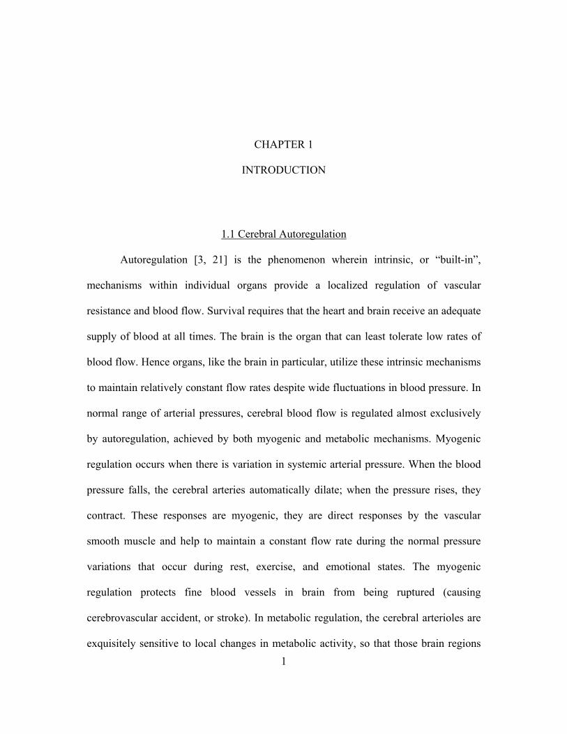
1.1 Cerebral Autoregulation
Autoregulation [3, 21] is the phenomenon wherein intrinsic, or “built-in”,
mechanisms within individual organs provide a localized regulation of vascular
resistance and blood flow. Survival requires that the heart and brain receive an adequate
supply of blood at all times. The brain is the organ that can least tolerate low rates of
blood flow. Hence organs, like the brain in particular, utilize these intrinsic mechanisms
to maintain relatively constant flow rates despite wide fluctuations in blood pressure. In
normal range of arterial pressures, cerebral blood flow is regulated almost exclusively
by autoregulation, achieved by both myogenic and metabolic mechanisms. Myogenic
regulation occurs when there is variation in systemic arterial pressure. When the blood
pressure falls, the cerebral arteries automatically dilate; when the pressure rises, they
contract. These responses are myogenic, they are direct responses by the vascular
smooth muscle and help to maintain a constant flow rate during the normal pressure
variations that occur during rest, exercise, and emotional states. The myogenic
regulation protects fine blood vessels in brain from being ruptured (causing
cerebrovascular accident, or stroke). In metabolic regulation, the cerebral arterioles are
exquisitely sensitive to local changes in metabolic activity, so that those brain regions
2
with the highest metabolic activity receive the most blood. The control mechanism in
this case is a result of the chemical environment created by the organ’s metabolism.
Some of the localized chemical conditions that promote vasodilation are (1) decreased
oxygen concentrations; (2) increased carbon dioxide concentrations; (3) decreased
tissue pH; and (4) the release of adenosine or K+ from the tissue cells [3]. Through these
chemical changes brain signals its blood vessels of its need for increased oxygen
delivery.
The cerebral autoregulation phenomenon has been well documented in animals
and humans. The understanding of this phenomenon is essential for development of
new strategies to prevent autonomic dysfunctions such as cognitive loss, falls, and
syncope, which are major causes of morbidity and mortality in elderly people [16]. One
of the means to study and analyze cerebral autoregulation is by identification of the
temporal relationship between beat-to-beat changes in mean arterial blood pressure
(MABP) and cerebral blood flow velocity (CBFV). Studies [18, 20, 25, 26, 28, 29, 30
and 44] of dynamic cerebral autoregulation have used different techniques to induce
rapid changes in MABP. These include sudden deflation of thigh cuffs, Valsalva
maneuvers, forced breathing, periodic squatting, or tilting of the whole body. Other
investigations involved spontaneous fluctuations in MABP to observe corresponding
transient changes in CBFV. There have been studies [13, 18, and 44] for evaluating the
role of autonomic neural activity versus other non-neural factors in autoregulation by
introducing ganglion blockade with trimethaphan, the infusion of which removes the
autonomic neural control of dynamic autoregulation.

3
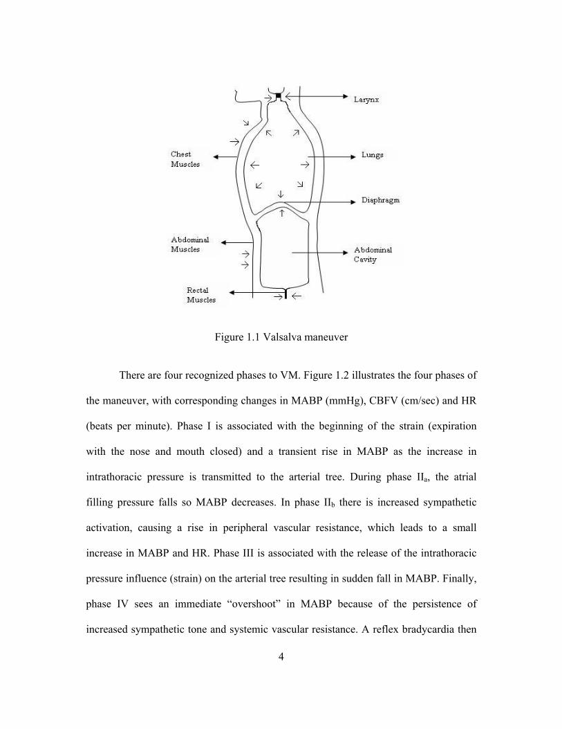
1.2 Valsalva Maneuver
Valsalva maneuver (VM) [3, 18, 19, 25, 26, 28, 29, and 30] is the term used to
describe an expiratory effort against a closed glottis (which prevents the air from exiting
the lungs) for at least 15 seconds by maintaining an expiratory pressure of
approximately 30 mmHg. It is approximately 45 seconds long and is also known as
Valsalva’s test and Valsalva’s method, after Antonio Maria Valsalva, a famous Italian
anatomist. Figure 1.1 illustrates a Valsalva maneuver. The maneuver mimics commonly
occurring events such as coughing, forceful defecation, or lifting of heavy weights. VM
increases the intrathoracic pressure and causes the abdominal muscles to tighten up,
squeezing the intestines and organs in abdominal cavity so that they press upward
against the diaphragm, compressing the chest cavity even more. Contraction of thoracic
cage compresses the lungs and causes a large rise in intrapleural pressure (the pressure
measured in the space between the lungs and thoracic wall) from approximately -3
mmHg to >150 mmHg. This results in the compression of the thoracic veins which
causes a fall in venous return and cardiac output, thus lowering arterial blood pressure.
The lowering of arterial pressure then stimulates the baroreceptor reflex, resulting in
tachycardia and increased total peripheral resistance. When the glottis is finally opened
and the air is exhaled, the cardiac output returns to normal, however, the blood pressure
is high as the total peripheral resistance is still elevated. The blood pressure is then
brought back to normal by the baroreceptor reflex, which causes a slowing of the heart
rate (HR).
4
Figure 1.1 Valsalva maneuver
There are four recognized phases to VM. Figure 1.2 illustrates the four phases of
the maneuver, with corresponding changes in MABP (mmHg), CBFV (cm/sec) and HR
(beats per minute). Phase I is associated with the beginning of the strain (expiration
with the nose and mouth closed) and a transient rise in MABP as the increase in
intrathoracic pressure is transmitted to the arterial tree. During phase IIa, the atrial
filling pressure falls so MABP decreases. In phase IIb there is increased sympathetic
activation, causing a rise in peripheral vascular resistance, which leads to a small
increase in MABP and HR. Phase III is associated with the release of the intrathoracic
pressure influence (strain) on the arterial tree resulting in sudden fall in MABP. Finally,
phase IV sees an immediate “overshoot” in MABP because of the persistence of
increased sympathetic tone and systemic vascular resistance. A reflex bradycardia then

5
results due to stimulation of arterial baroreceptors, and both MABP and HR return to
baseline values.
Figure 1.2 Phases (I through IV) associated with Valsalva maneuver shown in the mean
arterial blood pressure (MABP) subplot. The vertical arrow indicates the onset of the maneuver. The corresponding cerebral blood flow velocity (CBFV) and
heart rate (HR) changes are shown in the subsequent subplots.
VM is used as diagnostic tool to evaluate the condition of the heart and is done
as a treatment to correct abnormal heart rhythms or relieve chest pain. It has been used
as to test the integrity of autonomic function and may represent a dynamic challenge to
the autoregulatory mechanisms of cerebral circulation. Changes in cerebral
hemodynamics during the maneuver are mediated by both mechanical effects of the
changes in intrathoracic pressure and the elicited autonomic neural activity. The
differentiation between the mechanical effects and the autonomic effects has been done
using ganglion blockade with trimethaphan, the infusion of which essentially removes
the autonomic neural activity. The changes in cerebral hemodynamics during VM have

6
potentially significant clinical implications. If cerebral autoregulation is the process
regulating CBFV during phase IV of the maneuver, then the rapid rise in MABP should
be followed by a rapid rise in CBFV, which is quickly returned to baseline values by
dynamic autoregulation, before MABP returns to normal (Figure 1.2). In case of
patients with impaired autoregulation, the magnitude of MABP reduction during a
routine VM (phases IIa and III) is substantially greater than in normal subjects. This
would result in substantial reduction in CBFV which may ultimately lead to syncope.
Such effects can be also be seen in studies [13, 18, and 44] introducing ganglion
blockade by trimethaphan drug infusion for removal of the autonomic neural control of
dynamic autoregulation.
1.3 Previous Studies Involving Human Cerebral Circulation and its Modeling
Physiological modeling and system identification is aimed towards a better
understanding of the dynamics of various living systems. Modeling effort ranges from
graphic depiction of physiological process to mathematical emulation of realistic living
systems that unravels the mechanisms that underlie various complex physiological
functions. Physiological modeling strives to create a framework that would help with
the integration of experimental observations. A successful model also provides
guidance to new experiments, which may modify or generalize the model in turn
suggesting newer experiments.
In the context of human cerebral circulation under various pathophysiological
conditions, several studies [9, 10, 11, 13, 15, 16, 18, 20, 21, 23, 24, 25, 26, and 29] have
7
been done to understand pressure-flow velocity relationships using non-parametric
techniques such as transfer function analysis [5, 6, 12, and 44] using cross correlation
techniques [4, 5]. Non-linear analysis and neural network modeling studies of dynamic
cerebral autoregulation have also been conducted [7, 8]. Studies [28, 30, 41, 42, and 43]
involving frequency-domain and time-domain analysis of CBFV and its correlation with
MABP for assessing dynamics of autoregulation, developing indices for the degree and
quality of autoregulation and deriving clinical and physiological implications for
detection of autonomic dysfunction have all been well described and documented.
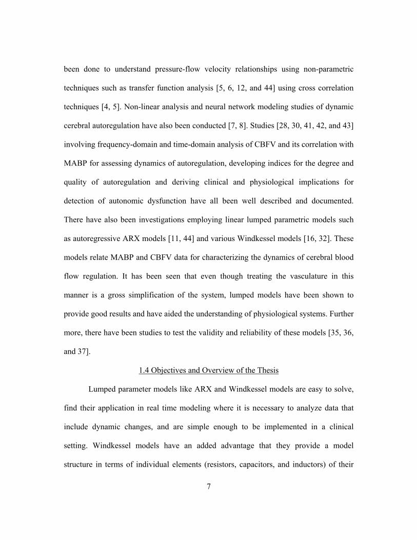
There have also been investigations employing linear lumped parametric models such
as autoregressive ARX models [11, 44] and various Windkessel models [16, 32]. These
models relate MABP and CBFV data for characterizing the dynamics of cerebral blood
flow regulation. It has been seen that even though treating the vasculature in this
manner is a gross simplification of the system, lumped models have been shown to
provide good results and have aided the understanding of physiological systems. Further
more, there have been studies to test the validity and reliability of these models [35, 36,
and 37].
1.4 Objectives and Overview of the Thesis
Lumped parameter models like ARX and Windkessel models are easy to solve,
find their application in real time modeling where it is necessary to analyze data that
include dynamic changes, and are simple enough to be implemented in a clinical
setting. Windkessel models have an added advantage that they provide a model
structure in terms of individual elements (resistors, capacitors, and inductors) of their

8
electrically analogous circuit. This makes it easier to extract the dynamic variation of
each of the elements from the measured data. It may also be possible to interpret
physiological changes with changes in the value of the elements.
The present study is focused on employing single input single output linear
lumped parametric models (ARX and Windkessel) to the data collected from normal
human subjects and computing the model parameters. The data consisted of beat-to-beat
mean arterial blood pressure (MABP, mmHg) considered as input to the model, and
cerebral blood flow velocity (CBFV, cm/sec) considered as output of the model. For
some models and modeling methodologies, the data consisted of cerebral perfusion
pressure (CPP, mmHg, estimated from MABP) and CBFV [18]. The measurement of
the data from the subjects was done while the subjects were performing Valsalva
maneuver with and without the use of trimethaphan for ganglion blockade, the infusion
of which essentially removes the autonomic neural activity.
Referring to previous studies involving human cerebral circulation and its
modeling in section 1.3, there have been no investigations in applying Windkessel
models to cerebral autoregulation data in conjunction with Valsalva maneuver for
ganglion blockade. Although there has been a previous study [44] involving ARX
models, it was limited to second order models only. Also under the same context, one
doesn’t find a comprehensive comparison of the performance of various models and
modeling techniques with respect to ARX models and Windkessel models. The main
objective of this study was to examine the relative performance and limitations of the
above mentioned linear modeling options and to demonstrate newer modeling

9
methodologies for them. All of these modeling methods rely on the assumption that the
dynamic autoregulatory mechanism can be approximated by a linear system, ignoring
all nonlinearities, like those related to fluid flow. It has been assumed that the MABP
and CBFV are correlated without taking into account any phase lag between them.
Another presumption is that the middle cerebral artery (MCA), where CBFV is
measured, does not change its diameter, and hence the words cerebral blood flow
velocity (CBFV) and cerebral blood flow (CBF) have been used interchangeably. Also,
effects due to changes in venous and intracranial pressure are not specifically included
in the data and the models where data was MABP and CBFV. These effects were
considered while estimating CPP from MABP and modeling CPP and CBFV.
Since for linear model estimation it is required that the input be persistently
exciting, another purpose of this study was to examine and establish the efficacy of
beat-to-beat blood pressure time sequence in serving as an input stimulus. Furthermore,
this involved investigating the possibility of using a shorter data segment of 1.5 minute
duration of changes in MABP for obtaining linear model estimation of cerebral
autoregulation. None of the studies in section 1.3 have involved this type of testing and
validation, and only one previous investigation has examined the use of 3 minute input
data [11]. Most of the previous studies have used the traditional 6 minutes duration of
pressure and flow data [12, 13, and 44].
The rest of this thesis is arranged in the following way. Chapter 2 presents the
experimental setup and protocol for the data collection and provides various model
structures and modeling techniques applied to the data. Chapter 3 presents the results

10
obtained from different modeling approaches and studies. Chapter 4 deals with the
discussion for the results and limitations. Finally, chapter 5 details the conclusions and
directions for future work.

11
CHAPTER 2
METHODS
This chapter presents the experimental setup, protocol for data collection and
various model structures and modeling methodologies applied to the data. All the data
analysis algorithms in this study were developed, tested and evaluated in MATLAB
(ver. 5.2 and ver. 6.5) and Simulink (ver. 5.0) environments, some of which are shown
in Appendix A.
2.1 Experimental Setup and Data Acquisition
2.1.1 Subjects
Data for the present study was obtained from ten healthy subjects, 8 men and 2
women, aged 29±6 years in supine resting position. No subject smoked, used
recreational drugs or had known medical problems. Subjects were screened carefully
with regard to their medical history and a physical examination with a 12-lead
Electrocardiogram (ECG). All subjects signed an informed consent form approved by
the Institutional Review Boards of the University of Texas Southwestern Medical
Center at Dallas and Presbyterian Hospital of Dallas.

12
2.1.2 Instrumentation
Heart rate (HR) was monitored continuously by ECG. The beat-to-beat mean
arterial blood pressure (MABP, mmHg) was measured non-invasively with finger
photoplethysmography (Finapres Ohmeda, Amsterdam, Netherlands). The cerebral
blood flow velocity (CBFV, cm/sec) was recorded from the middle cerebral artery
(MCA) with transcranial Doppler ultrasonography (TCD). A 2-MHz probe (Multiflow
DWL, Elektronische Systeme, Sipplingen, Germany) was placed over the subject’s
temporal window and fixed at a constant angle with a probe holder to secure the probe
position during the experiments. This technique allows non-invasive and repeatable
estimates of changes in CBFV on a beat-to-beat basis.
2.1.3 Experimental Protocol
All experiments were performed in the morning at least 2 hours after a light
breakfast in a quiet environmentally controlled laboratory with an ambient temperature
of 25 °C. The subjects were asked to refrain from heavy exercise and caffeinated or
alcoholic beverages at least 24 hours before the tests. After at least 30 minutes of supine
rest, 6 minutes of baseline data were collected during spontaneous breathing. This data
collection was repeated again after approximately 1 hour to test the reproducibility of
MABP and CBFV. Then, the subjects performed a Valsalva maneuver (VM) with an
expiratory strain of 30 mmHg for 15 seconds. The strain pressure during the VM was
monitored by a sphygmomanometer (Tycos, Arden, NC, USA). Typical changes in
MABP, HR and CBFV during the maneuver were observed in all subjects before
ganglion blockade. After performance of the baseline VM, intravenous infusion of
13
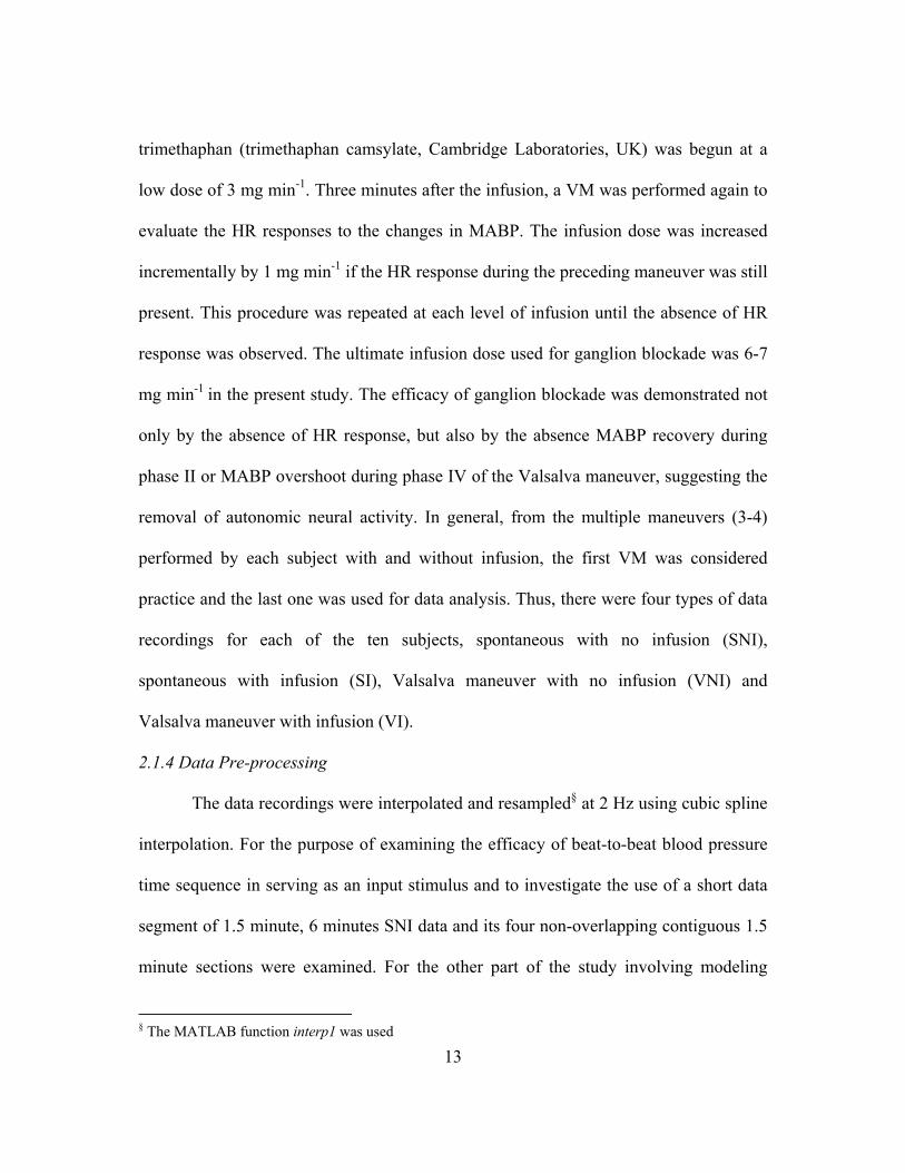
trimethaphan (trimethaphan camsylate, Cambridge Laboratories, UK) was begun at a
low dose of 3 mg min-1. Three minutes after the infusion, a VM was performed again to
evaluate the HR responses to the changes in MABP. The infusion dose was increased
incrementally by 1 mg min-1 if the HR response during the preceding maneuver was still
present. This procedure was repeated at each level of infusion until the absence of HR
response was observed. The ultimate infusion dose used for ganglion blockade was 6-7
mg min-1 in the present study. The efficacy of ganglion blockade was demonstrated not
only by the absence of HR response, but also by the absence MABP recovery during
phase II or MABP overshoot during phase IV of the Valsalva maneuver, suggesting the
removal of autonomic neural activity. In general, from the multiple maneuvers (3-4)
performed by each subject with and without infusion, the first VM was considered
practice and the last one was used for data analysis. Thus, there were four types of data
recordings for each of the ten subjects, spontaneous with no infusion (SNI),
spontaneous with infusion (SI), Valsalva maneuver with no infusion (VNI) and
Valsalva maneuver with infusion (VI).
2.1.4 Data Pre-processing
The data recordings were interpolated and resampled§ at 2 Hz using cubic spline
interpolation. For the purpose of examining the efficacy of beat-to-beat blood pressure
time sequence in serving as an input stimulus and to investigate the use of a short data
segment of 1.5 minute, 6 minutes SNI data and its four non-overlapping contiguous 1.5
minute sections were examined. For the other part of the study involving modeling
§ The MATLAB function interp1 was used

14
methodologies and their comparison, first 1.5 minute section of the 6 minute SNI
recording, and approximately 90 seconds (1.5 minute) of SI, VNI and VI data
recordings were used. Prior to any analysis, all data sequences were first detrended∗ by
removing their mean values, and then normalized by the range of time series (maximum
value of the sequence minus minimum value of the sequence). Figure 2.1 through
Figure 2.4 illustrate approximately 90 seconds recordings of MABP and CBFV for
subject number 1 for all the four (SNI, SI, VNI, and VI) data conditions.
Figure 2.1 Spontaneous with no infusion (SNI) mean arterial blood pressure (MABP)
and cerebral blood flow velocity (CBFV) data
∗ The MATLAB function dtrend was used

15
Figure 2.2 Spontaneous with infusion (SI) mean arterial blood pressure (MABP) and
cerebral blood flow velocity (CBFV) data
Figure 2.3 Valsalva maneuver with no infusion (VNI) mean arterial blood pressure
(MABP) and cerebral blood flow velocity (CBFV) data

16
Figure 2.4 Valsalva maneuver with infusion (VI) mean arterial blood pressure (MABP)
and cerebral blood flow velocity (CBFV) data
2.2 Modeling Methodologies
This section describes the two types of modeling approaches (ARX and
Windkessel) employed to the data collected as mentioned in the previous section.
Section 2.2.1 discusses the ARX modeling technique and modeling schemes associated
with it. Section 2.2.2 details Windkessel estimation and various types of Windkessel
models employed in the present study, section 2.2.3 discusses different modeling
schemes associated with them.
2.2.1 ARX Model Estimation
For linear system parametric identification of an autoregressive ARX model [1,
2, 14, 27, and 44], the model describes the relationship between input signal, output
signal, and disturbance signal or noise, through a set of linear difference equations

17
where the output at a given time t is computed as a linear combination of the current
and past outputs and the current and past inputs. In general the structure for ARX
identification is,
)().()().()( kqHkuqGky ε+= (2.1)
where y is the output, u is the input and ε is the noise, k is the sample number (instance)
and q is the index of the domain in which the model transfer function is analyzed. G is
the process model, which represents the causal relationship between the deterministic
input u and output y to the model, H is the noise model.
In many cases, the effect of noise on the model output may be insignificant as
compared to the input signal. Hence, it is often not necessary to include an accurate
noise model in the system modeling such as in the study of cerebral autoregulation [8,
11, and 12]. Thus, for a single input, single output model the structure (excluding the
noise model H) can be represented as,
)()()(01
ikubikyakym
ii
n
ii −=−+ ∑∑
==
(2.2)
∑
∑
=
−
=
−
+= n
i
ii
m
i
ii
qa
qbqG
1
0
1)( (2.3)
The transfer function in Z-domain for the above model structure G(q) would be,
nn
mm
zazazbzbb
zG −−
−−
++++++
=......1......
)( 11
110 (2.4)
In ARX model estimation, the model structure is set a priori, but with unknown model
order (i.e. the upper bound on m and n). The model identification is reduced to

18
estimating the model order and its parameters (ai and bi) using input and output data that
give the best agreement between model’s (computed or predicted) output and the
measured one. There are various criteria that are used to select a model and its order,
such as mean squared error (MSE), Akaike’s index or final prediction error (FPE) [22].
In case of this study, the MSE value between the measured and predicted output was
used.
With respect to selection and restriction of the orders m and n of the ARX
model, there were two modeling schemes that have been followed in this study§. They
will be referred to as ARX-1 and ARX-2 modeling schemes.
2.2.1.1 ARX-1 Modeling Scheme
The block diagram in Figure 2.5 illustrates the ARX-1 modeling scheme for
each subject for all the four data conditions. All the possible causal ARX models with
orders m and n ranging from 1 to 10 (a total of 55 models) were considered using
MABP (u1) as the input and CBFV (v1) as the output. The mean squared error (MSE)
value between the predicted output (v2) from each of these models and v1 was then
calculated based on the following general equation,
( ) ( )[ ]
n
Ln
iyx
L
ivivMSE
∑=
−= 0
2
(2.5)
where vx and vy are the two data sequences for which the MSE value is to be calculated
and Ln is the length of the data sequences.
§ The MATLAB function arx was used

19
The model having the smallest MSE value was selected as the best. This way, for each
of the 10 subjects, there were four best models generated, one for each of the SNI, SI,
VNI, and VI conditions of the data respectively.
Figure 2.5 ARX-1 modeling scheme
2.2.1.2 ARX-2 Modeling Scheme
The block diagram in Figure 2.6 illustrates the ARX-2 modeling scheme for
each subject for all the four data conditions. In this type of modeling scheme, ARX
model orders m and n were restricted to be 1, 2, and 3, utilizing MABP (u1) as the input
and CBFV (v1) as the output. This way, for each of the 10 subjects, for each of the SNI,
SI, VNI, and VI conditions of the data, there were three models (one 1st order, one 2nd
order, and one 3rd order model) generated. Hence, the total number of models for each
subject was 12. The mean squared error (MSE) value between the predicted output (v2)
MABP Measured Input (u1)
CBF V Measured
Output (v1)
Estimating Possible Causal Models with Combinations of m = 1 to 10, n = 1 to 10 in the Transfer Function (55 Models)
Calculation of MSE between v1 and v2
for the Models Predicted Output v2
ARX Estimation
m and n are numerator and denominator orders
Best Model with Minimum MSE

20
from each of these models and v1 was then calculated based on equation 2.5. The
rationale behind restricting the model order was to provide a comparison between the
performance of ARX and Windkessel models (Windkessel models generally are limited
to 1st, 2nd and 3rd order model structures). Also, a comparison between the performances
of ARX-1 and ARX-2 modeling schemes would provide an insight in reason behind
fitting lower order models to physiological data and trying to select models of order as
high as 10.
Figure 2.6 ARX-2 modeling scheme
2.2.2 Windkessel Model Estimation
Windkessel and similar lumped models are often used to represent blood flow
and pressure in arterial system and to capture the dynamics of cerebral circulation [17,
31, 32, 33, 34, 35, 36, 37, 38, 39, and 40]. These lumped models can be derived from
electrical circuit analogies where current (i) represents blood flow and voltage (v)
represents pressure. Resistances (R) represent arterial and peripheral resistance that
MABP Measured Input (u1)
CBF V Measured
Output (v1)
Estimating Models with m and n restricted to be 1, 2, or
3 in the Transfer Function
Calculation of MSE between v1 and v2
for the Model Predicted Output v2
ARX Estimation
m and n are numerator and denominator orders

21
occurs as a result of viscous dissipation inside vessels, capacitors (C) represent volume
compliance of the vessels that allows them to store significant amounts of blood, and
inductors (L) represent inertia of the blood flow in vessels.
The Windkessel model was originally put forward by Stephen Hales in 1733 and
further developed by Otto Frank in 1899. Frank used Windkessel model to describe
blood flow in the heart and systemic arteries, modeling the arterial system as a
compliant reservoir fed by the heart (Cs), driving a simple resistive load (Rs) modeled as
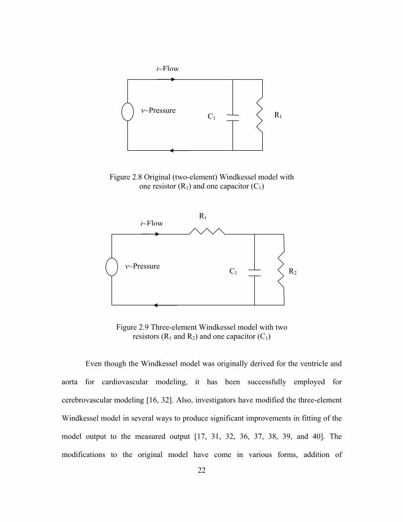
resistance to the outflow (Figure 2.7). The original (two-element) Windkessel model
(Figure 2.8) comprised an electric circuit with one resistor and one capacitor; where the
capacitor represented the compliance of the large arteries while the resistor represented
the resistance of the small arteries and arterioles (so called resistance vessels). The two-
element Windkessel model was later extended to the three-element Windkessel model,
which had two resistors and a capacitor (Figure 2.9). The additional resistor was
thought to represent the characteristic impedance of aorta and the large compliance
vessels. The three-element model is and has been widely used and accepted.
Figure 2.7 Frank’s simple Windkessel model of arterial vascular system
Inflow
Outflow
Peripheral Resistance Rs
Compliant Reservoir Cs
22
Figure 2.8 Original (two-element) Windkessel model with one resistor (R1) and one capacitor (C1)
Figure 2.9 Three-element Windkessel model with two resistors (R1 and R2) and one capacitor (C1)
Even though the Windkessel model was originally derived for the ventricle and
aorta for cardiovascular modeling, it has been successfully employed for
cerebrovascular modeling [16, 32]. Also, investigators have modified the three-element
Windkessel model in several ways to produce significant improvements in fitting of the
model output to the measured output [17, 31, 32, 36, 37, 38, 39, and 40]. The
modifications to the original model have come in various forms, addition of
R1
R2 C1
i~Flow
v~Pressure
R1 C1
i~Flow
v~Pressure

23
capacitances to mimic local and distal compliances, addition of resistor-capacitor
combinations to expand the model to more finite levels like arterioles, capillaries and
veins and addition of inductance-resistance combination to add inertial effect associated
with long vessels. Although these modifications generated better results over the
original Windkessel model, their physiological interpretations were not always obvious
and apparent. Windkessel models are easy to understand and simple in their structure,
however, these models include a number of parameters (resistors, capacitors, and
inductors), and it is not obvious how to estimate the parameters from measurements of
just blood flow and pressure. Generally the estimation of these parameters depends on
minimization or maximization of a cost-function (a function of time or frequency) to
either fit the model time-domain output to the measured time-domain output, or match
the measured and model frequency responses.
The present study employs the basic three-element Windkessel model and four
of its modified versions, which have shown significant improvements in fitting of the
model output to the measured output in previous cardiovascular and cerebrovascular
modeling studies. Their transfer functions using Laplace transform (S-domain) have
been analyzed considering MABP as input to the model and CBFV as output to the
model.

24
2.2.2.1 Model 1: Windkessel 3-Element Model [16, 21, 32, 33, 34, 35, 37, 38]
Figure 2.11 Windkessel 3-element model
Figure 2.11 illustrates the structure for the basic 3-element Windkessel model
(Model 1), with input MABP analogous to voltage (v) and output CBFV analogous to
current (i). The transfer function in S-domain for Model 1 in terms of its parameters R1,
R2, and C1, is,
( )
( )
[ ]( )[ ]21211
211
1)(RRRRsC
RsC
sv
sisg++
+== (2.6)
R1
R2 C1
i~CBFV
v~MABP
25
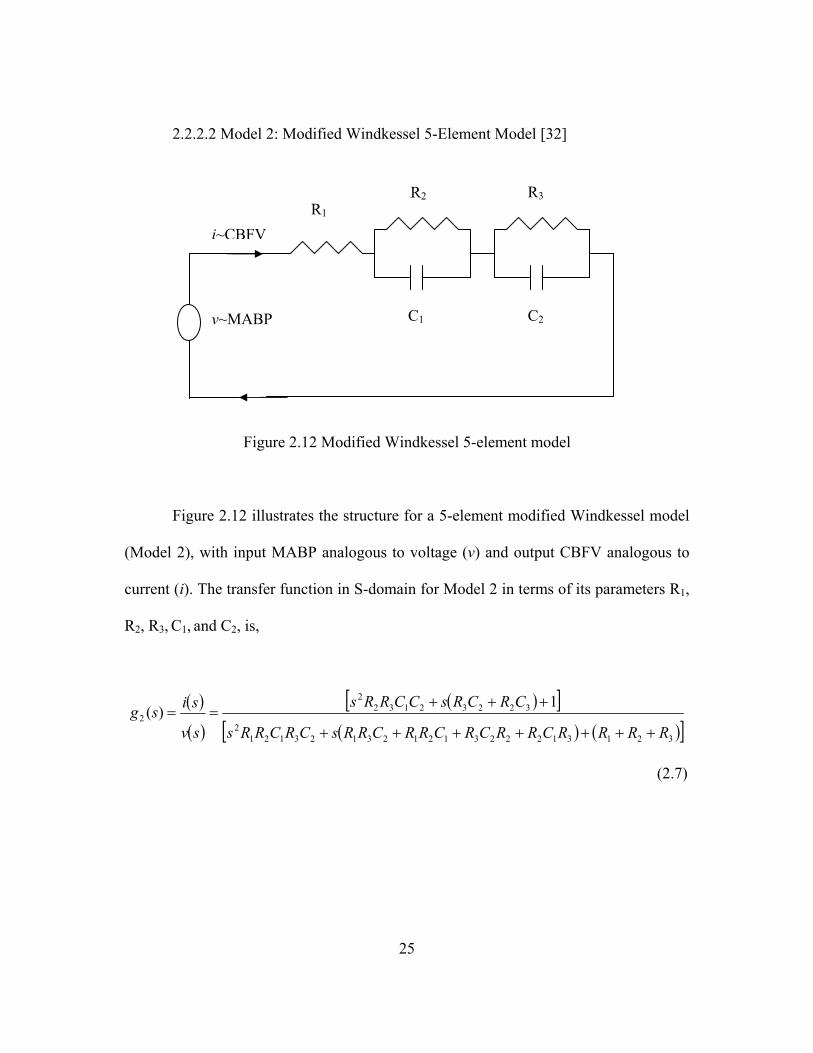
2.2.2.2 Model 2: Modified Windkessel 5-Element Model [32]
Figure 2.12 Modified Windkessel 5-element model
Figure 2.12 illustrates the structure for a 5-element modified Windkessel model
(Model 2), with input MABP analogous to voltage (v) and output CBFV analogous to
current (i). The transfer function in S-domain for Model 2 in terms of its parameters R1,
R2, R3, C1, and C2, is,
( )
( )
( )[ ]( ) ( )[ ]32131222312123123121
2
322321322
21
)(RRRRCRRCRCRRCRRsCRCRRs
CRCRsCCRRs
sv
sisg+++++++
+++==
(2.7)
R1 i~CBFV
v~MABP
R2 R3
C1 C2
26
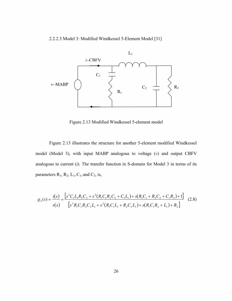
2.2.2.3 Model 3: Modified Windkessel 5-Element Model [31]
Figure 2.13 Modified Windkessel 5-element model
Figure 2.13 illustrates the structure for another 5-element modified Windkessel
model (Model 3), with input MABP analogous to voltage (v) and output CBFV
analogous to current (i). The transfer function in S-domain for Model 3 in terms of its
parameters R1, R2, L1, C1, and C2, is,
( )
( )
( ) ( )[ ]( ) ( )[ ]21211122111
212211
3
2122111122112
22113
31)(
RLRCRsLCRLCRsLCRCRs
RCCRCRsLCCRCRsCRLCs
sv
sisg+++++
++++++== (2.8)
L1
R2
C1
i~CBFV
v~MABP C2 R1

27
2.2.2.4 Model 4: Modified Windkessel 5-Element Model [39]
Figure 2.14 Modified Windkessel 5-element model
Figure 2.14 illustrates the structure for yet another 5-element modified
Windkessel model (Model 4), with input MABP analogous to voltage (v) and output
CBFV analogous to current (i). The transfer function in S-domain for Model 4 in terms
of its parameters R1, R2, L1, C1, and C2, is,
( )
( )
( )[ ]( ) ( ) ( )[ ]211211122122111
212211
3
2122112
12213
41)(
RRLRCRRCRsLCRLCRsLCRCRs
RCCRsLCsCCRLs
sv
sisg+++++++
++++==
(2.9)
L1
R2 C1
i~CBFV
v~MABP C2
R1

28
2.2.2.5 Model 5: Modified Windkessel 4-Element Model [17, 38]
Figure 2.15 Modified Windkessel 4-element model
Figure 2.15 illustrates the structure for a 4-element modified Windkessel model
(Model 5), with input MABP analogous to voltage (v) and output CBFV analogous to
current (i). The transfer function in S-domain for Model 5 in terms of its parameters R1,
R2, L1, and C1, is,
( )
( )
( )[ ]( ) ( )[ ]2112111211
2
121111212
5 )(RRLRLRsLRCRs
RRRCLsLRCs
sv
sisg+++
+++== (2.10)
2.2.3 Windkessel Modeling Schemes
From the section 2.2.2 it is relatively clear that the Windkessel models are easy
to understand and simple, yet defined in their structure. However, these models include
a number of parameters (R, L, and C), and the real challenge of the model identification
is the estimation of these parameters from the measurements of just MABP and CBFV.
In pervious investigations [16, 21, 31, 32, 34, 35, 37, and 38] the extraction of these
L1
R2
i~CBFV
v~MABP C1
R1

29
parameters was done by minimization or maximization of a cost-function, which may
be a function of time or frequency. The present study involves parameter selection by a
two-phase optimization§ of the parameters of a Windkessel model. This optimization is
done by minimization of the MSE in frequency domain for the measured and predicted
impedance curves, and MSE in time domain for the measured and predicted outputs.
They are referred as frequency-domain optimization phase and time-domain
optimization phase respectively. The advantage of this two phase optimization process
is that it converges to final values of the parameters which yield better time-domain fit
of the model output and result in lower time-domain MSE value between the measured
and the model output, as compared to single stage parameter extraction techniques
similar to those used in previous investigations.
For frequency-domain optimization phase, first an impedance curve for the
measured data (detrended and normalized MABP and CBFV) was generated. This was
done by finding the cross-correlation, Syx, of CBFV and MABP sequences, and the
auto-correlation, Sxx, of MABP. Then by Welch’s averaged, modified periodogram
method*, a 512 point fast Fourier transform (FFT) of Syx and Syx was calculated with 50
percent overlap, using a Hanning window and a sampling frequency of 2 Hz. The
measured impedance curve Zm was calculated from dividing the absolute value
(modulus) of the FFT of Syx by the absolute value of the FFT of Sxx. In the equations 2.6
through 2.10, replacing the complex variable s in the each of the transfer function for
the five Windkessel models, by jω, where j is imaginary number ( 2 1− ) and ω is
§ The MATLAB function fminimax was used * The MATLAB function psd was used

30
frequency (rad/sec), would present the transfer function as a function of ω with
unknown values of parameters. Taking the absolute value (modulus) of this transfer
function would yield the predicted impedance curve for the model, Zp. Essentially, the
frequency-domain optimization is selection of the parameters of the model in order to
fit Zp to Zm, such that the MSE value between Zm and Zp is minimized.
Time-domain optimization phase involves selecting those parameters, R, C and
L of a Windkessel model, which minimize the MSE value between the measured time
domain output (CBFV) and predicted (model) time domain output, for fitting the
predicted output to the measured one. To calculate the predicted time domain output,
the estimated model was subjected to the measured time domain input (MABP).
2.2.3.1 Optimization Algorithm
This section provides an overview of the optimization method used in the
present study. For both frequency-domain and time-domain optimization phases,
parameters of the Windkessel models were estimated using a constrained optimization
technique. In this technique, a multivariable function is minimized, starting at an initial
estimate. The value of the variables (parameters R, C, and L of the model) are subject to
constraints, in terms of lower and upper bounds that they can attain. The lower and the
upper bound values are decided keeping physiologically considerations in mind and
referring pervious cerebral blood flow modeling studies. In the present study, for the
part which involves analyzing the five Windkessel models for fitting them to the subject
data, the lower and the upper boundary values were 0.1 and 50 for the frequency-
domain optimization phase and 0.01 and 100 for the time-domain optimization phase

31
respectively, for every parameter. The difference in the boundary values for the two
phases accounts for the situation when the frequency-domain optimization phase yields
parameter estimates which are close to its boundary values, particularly to the upper
boundary value. This allows the time-domain optimization phase to start with an initial
estimate that is approximately at the midpoint of the range of its boundary values, and
hence result in better parameter estimates. This strategy is advantageous in case where
the two phases are sequential and final estimates of one phase act as initial estimates for
the subsequent phase.
In constrained optimization, the general aim is to transform the problem into an
easier sub-problem that can then be solved and used as the basis of an iterative process.
In this way the constrained problem is solved using a sequence of parameterized
unconstrained optimizations, which in the limit (of the sequence) converge to the
constrained problem. This method is commonly referred to as Sequential Quadratic
Programming (SQP) method, since a QP sub-problem is solved at each major iteration
(also known as Iterative Quadratic Programming, Recursive Quadratic Programming,
and Constrained Variable Metric methods) [2].
Constrained methods use the solution of a sub-problem to yield a search
direction in which the solution is estimated to lie. The minimum along the path formed
from this search direction is generally approximated using a search procedure. In the
present study, this search procedure was a cubic polynomial method, where a function
evaluation is made at every iteration. At each iteration an update is performed when a
new point is found that results in a lower value of the multivariable function being

32
minimized. Value of each function parameter is also updated by a step at every
iteration. If this step does not result into a lower function value, then further reduction
in the step is done to form a new step, Usual method for this reduction is to use
bisection, i.e., to continually halve the step length until a reduction is achieved in the
function output. The values of the optional parameters like the step size, maximum
number of iterations, maximum number of function evaluations, and termination
tolerance on the constraint violation can be provided before the start of the optimization
to improve the efficiency and accuracy of the process. More details about the
optimization algorithm can be found in [2].
While SQP method has been implemented and tested over a large number of test
problems, it has certain limitations. For instance, the function to be minimized must be
continuous and the optimization may result in only the local solutions. Also, the method
is very sensitive to the initial estimates. Based on the number of parameters optimized
and the sequence of performing the frequency-domain and time-domain optimization
phases, three types of Windkessel modeling schemes were obtained. They will be
referred to as Windkessel-1, Windkessel-2 and Windkessel-3 modeling schemes.
2.2.3.2 Windkessel-1 Modeling Scheme
The Windkessel-1 relies on the approximation that the resistance parameter R1
for the each of the five Windkessel models can be extracted from the highest frequency
point of the measured impedance curve Zm. As discussed in section 2.2.3, in the
equations 2.6 through 2.10, replacing the complex variable s in the each of the transfer
function for the five Windkessel models, by jω, where j is imaginary number ( 2 1− )
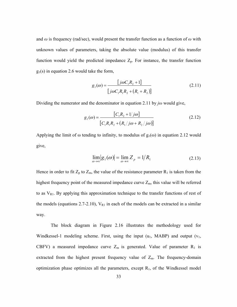
33
and ω is frequency (rad/sec), would present the transfer function as a function of ω with
unknown values of parameters, taking the absolute value (modulus) of this transfer
function would yield the predicted impedance Zp. For instance, the transfer function
g1(s) in equation 2.6 would take the form,
[ ]
( )[ ]21211
211
1)(
RRRRCj
RCjg++
+=
ω
ωω (2.11)
Dividing the numerator and the denominator in equation 2.11 by jω would give,
[ ]( )[ ]ωω
ωω
jRjRRRC
jRCg
21211
211
1)(
++
+= (2.12)
Applying the limit of ω tending to infinity, to modulus of g1(ω) in equation 2.12 would
give,
11 1lim)(lim RZg p ==∞→∞→ ωω
ω (2.13)
Hence in order to fit Zp to Zm, the value of the resistance parameter R1 is taken from the
highest frequency point of the measured impedance curve Zm, this value will be referred
to as VR1. By applying this approximation technique to the transfer functions of rest of
the models (equations 2.7-2.10), VR1 in each of the models can be extracted in a similar
way.
The block diagram in Figure 2.16 illustrates the methodology used for
Windkessel-1 modeling scheme. First, using the input (u1, MABP) and output (v1,
CBFV) a measured impedance curve Zm is generated. Value of parameter R1 is
extracted from the highest present frequency value of Zm. The frequency-domain
optimization phase optimizes all the parameters, except R1, of the Windkessel model

34
being analyzed, for least square fitting of Zp to Zm (minimizing the MSE between the
two). For the 3-element Windkessel model (Model 1), the initial estimates (Initial
Estimates 1) of the parameters being optimized for frequency-domain optimization were
taken from the results of a pervious cerebral blood flow modeling study [16]. For the
rest of the four Windkessel models, the initial estimate for every parameter was the
middle point value of the range of the boundary condition (constraint) for the
optimization of that parameter (section 2.2.3.1). Thus, at the end of the optimization,
VR1 and value of every frequency-domain optimized parameter of the Windkessel
model (Estimate 1) is given.
The time-domain optimization phase is the process of least square fitting of the
model output to the measured output, by optimizing the parameters, except R1, starting
from the Estimate 1 values (Initial Estimates 2 = Estimate 1). At the end of the
optimization, VR1, and of every time-domain optimized parameter of the Windkessel
model (Estimate 2) is given. The Estimate 2 along with VR1, are taken as the final
values of the model parameters. Based on equation 2.5, MSE is calculated between v1
and the predicted output v2 of model with these final values. The Windkessel-1
modeling scheme utilizes the value of parameter R1 (VR1, extracted from Zm) in both the
frequency-domain and time domain optimizations, but R1 is essentially never optimized.
This modeling scheme was applied to all the 10 subjects’ data, to all the four data
conditions (SNI, SI, VNI, and VI) for each subject, and for all the five Windkessel
models.

35
Figure 2.16 Windkessel-1 modeling scheme
2.2.3.3 Windkessel-2 Modeling Scheme
The block diagram in Figure 2.17 illustrates the methodology used for
Windkessel-2 modeling scheme. First, using the input (u1, MABP) and output (v1,
CBFV) a measured impedance curve Zm was generated. Value of parameter R1 is
extracted from the highest present frequency value of Zm, as discussed in section
2.2.3.2. The frequency-domain optimization phase optimizes all the parameters, except
MABP Measured Input (u1)
CBFV Measured
Output (v1)
Extracting VR1 from Highest Frequency Point of Zm
Estimate 1
Predicted Output v2
Generating Measured Impedance Curve, Zm
Frequency-Domain Optimization Optimizing all the Parameters, Except R1, by Fitting Predicted
Impedance Curve Zp to Zm
Time-Domain Optimization Optimizing all the Parameters,
Except R1, by Fitting Model Output to the Measured Output
VR1, Estimate 2
Initial Estimates 2
Initial Estimates 1
Calculation of MSE between v1 and v2
for the Model
u1, v1, VR1
VR1
Measured Input u1
Final Estimate of
Model Parameters

36
R1, of the Windkessel model being analyzed, for least square fitting of Zp to Zm
(minimizing the MSE between the two). For the 3-element Windkessel model (Model
1), the initial estimates (Initial Estimates 1) of the parameters being optimized for
frequency-domain optimization were taken from the results of a pervious cerebral blood
flow modeling study [16]. For the rest of the four Windkessel models, the initial
estimate for every parameter was the middle point value of the range of the boundary
condition (constraint) for the optimization of that parameter (section 2.2.3.1). Thus at
the end of the optimization, VR1 and value of every frequency-domain optimized
parameter of the Windkessel model (Estimate 1) is given.
The time-domain optimization phase in this scheme optimizes all the parameters,
including R1, starting from VR1, and Estimate 1 values (Initial Estimates 2 = [VR1,
Estimate 1]) for least square fitting of the model output to the measured output. At the
end of the optimization, the numerical value of every time-domain optimized parameter
of the Windkessel model (Estimate 2) is given, which is taken as the final value of that
model parameter. Based on equation 2.5, MSE is calculated between v1 and the
predicted output v2 of model with these final values. The Windkessel-2 modeling
scheme utilizes the value of parameter R1 (VR1, extracted from Zm) in the frequency-
domain optimization, and as initial estimate for the time domain optimization. This
modeling scheme was applied to all the 10 subjects’ data, to all the four data conditions
for each subject, and for all the five Windkessel models.

37
Figure 2.17 Windkessel-2 modeling scheme
2.2.3.4 Windkessel-3 Modeling Scheme
In Windkessl-3 scheme, simultaneous frequency-domain and time-domain
optimization is performed, in contrast to sequential processes of Windkessel-1 and
Windkessel-2 schemes where first optimization in frequency-domain and then in time-
domain is performed. Hence in this type of modeling scheme, simultaneous
MABP Measured Input (u1)
CBFV Measured
Output (v1)
Extracting VR1 from Highest Frequency Point of Zm
Predicted Output v2
Generating Measured Impedance Curve, Zm
Frequency-Domain Optimization Optimizing all the Parameters, Except R1, by Fitting Predicted
Impedance Curve Zp to Zm
Time-Domain Optimization Optimizing all the Parameters, Including R1, by Fitting Model Output to the Measured Output
Estimate 2 Initial
Estimates 2
Calculation of MSE between v1 and v2
for the Model
Estimate 1
Initial Estimates 1
VR1
u1, v1 Measured Input u1
VR1
Final Estimate of
Model Parameters

38
minimization of the MSE in frequency domain for the measured and predicted
impedance curves, and MSE in time domain for the measured and predicted outputs, is
done§. For this purpose, frequency and time domain MSE values are weighed by certain
weighting coefficients for the optimization, such that the sum of the two weighting
coefficients (one for frequency-domain MSE, Wf, another for time-domain MSE, Wt) is
1. Hence Wt is varied from 0.1 to 0.9 in steps of 0.1, whereas Wf = 1- Wt. From all of
these 9 combinations of Wt and Wf (including one where Wt = Wf = 0.5), selection of
the model parameters is done for the combination which produces the minimum time-
domain MSE value.
The block diagram in Figure 2.18 illustrates the methodology used for
Windkessel-3 modeling scheme. Using the input (u1, MABP) and output (v1, CBFV) a
measured impedance curve Zm was generated. The frequency-domain MSE between Zp
and Zm is calculated. The time-domain MSE between the predicted (model) output and
the measured output is also calculated. The optimization process minimizes the
weighted frequency and time domain MSE values simultaneously, and for the 9
combination of Wt and Wf, generates 9 sets of optimized parameters for the Windkessel
model under analysis. Then for each of these 9 sets of model parameters, based on
equation 2.5, time-domain MSE value is calculated between v1 and the predicted output
v2 of model. The set of parameters yielding minimum MSE value is taken as the final
estimate. This modeling scheme was applied to all the 10 subjects’ data, to all the four
data conditions for each subject, and for only the 3-element Windkessel model (Model
§ The MATLAB function fgoalattain was used

39
1). The initial estimates of the parameters being optimized were taken from the results
of a pervious cerebral blood flow modeling study involving Model 1 [16] and the lower
and the upper boundary values were respectively 0.01 and 100 for the optimizations.
Figure 2.18 Windkessel-3 modeling scheme
MABP Measured Input (u1)
CBFV Measured
Output (v1)
Predicted Output v2
Generating Measured Impedance Curve, Zm
Frequency-Domain Optimization Optimizing all the Parameters to Minimize Wf x MSE, by Fitting
Predicted Impedance Curve Zp to Zm
Time-Domain Optimization Optimizing all the Parameters to Minimize Wt x MSE, by Fitting Model Output to the Measured
Output
9 Sets of Parameter Estimates
Initial Estimates
Calculation of MSE between v1 and v2
for the Models
Weight Wf = 1- Wt Weight Wt = 0.1to 0.9
u1
u1, v1
Final Estimate with Minimum MSE

40
2.3 Establishing the Adequacy and Efficacy of 1.5 Minute MABP as Input Stimulus
For a linear model estimation it is required that the input be persistently exciting.
This section focuses on that part of study which is aimed to establish if the MABP is
adequately persistently exciting to properly estimate a linear model. In addition the
possibility of using a short data segment of 1.5 minute of changes in MABP for linear
model identification was examined. This is of relevance because various linear
modeling investigations involve use of a pathophysiological condition, like Valsalva
maneuver with and without ganglion blockade in the present study, which last
approximately 1.5 minute long.
The data used for this part of the study was spontaneous no infusion (SNI) data.
The aim was to prove that beat-to-beat MABP sequence is as effective as pseudo
random binary sequence (PRBS). This is of importance, because PRBS is a very wide
bandwidth signal and is considered persistently exciting. The study was based on
parametric identification of autoregressive ARX and Windkessel models. In case of
Windkessel models, the study was done by performing Monte-Carlo simulations
(random-walk method) for 1000 trials.
2.3.1 ARX Models
This study was based on ARX-1 modeling scheme. The block diagrams in Figure
2.19 and Figure 2.20 illustrate the steps for the applied methodology for analysis of the
ARX models for each of the 10 subjects. All the possible causal ARX models with
numerator and denominator order (m and n) ranging from 1 to 10 (a total of 55 models)
were considered using measured MABP (u1) as input and CBFV (v1) data as output

41
sequences. Based on equation 2.5, the MSE values between the predicted output (v2)
from these models and v1 were then calculated and the model having smallest MSE
value was selected as the best. This model will be referred to as Ma.
For the next two steps, Ma was treated as an unknown system. In step 2 of
investigation, model Ma was subjected to PRBS signal (u2) with minimum value of -1,
maximum value of +1, initial seed equal to zero and sample time equal to 0.5 seconds to
obtain the computed output (v3). All the possible causal ARX models with m and n
ranging from 1 to 10 (a total of 55 models) were fitted to u2 and v3. Based on equation
2.5, the MSE values between the predicted output (v4) of the estimated models and v3
(used to estimate the model parameters) were then calculated and the model with the
smallest MSE value was selected as the best, Me1. The third step involved subjecting Ma
to measured MABP (u1) instead of PRBS. Again, all the 55 possible valid ARX models
with m and n ranging from 1 to 10 were fitted to u1 and resulting Ma output (v5). From
equation 2.5, MSE between the predicted output (v6) from these models and computed
output (v5) was then calculated and the model having smallest MSE value was selected
as the best, Me2.
In order to compare all three models, Ma, Me1 and Me2, in the fourth and final
step of the study, Me1 and Me2 were excited with the measured MABP as input (u1) and
MSE values for the predicted outputs (v2 for Ma , v7 for Me1, and v8 for Me2) and
measured CBFV (v1) were calculated based on equation 2.5. This four-step study was
carried out for all 10 subjects, first with 6 minutes SNI data, and then with all the four
non-overlapping contiguous 1.5 min sections of the measured 6 minute SNI data.

42
Figure 2.19 Steps 1 to 3 for the ARX modeling methodology for establishing the adequacy and efficacy of 1.5 minute MABP as input stimulus

43
Figure 2.20 Step 4 for the ARX modeling methodology for establishing the adequacy and efficacy of 1.5 minute MABP as input stimulus
2.3.2 Monte-Carlo Simulations for Windkessel Modeling Schemes
This study was based on performing 1000 trials Monte-Carlo simulation for
Windkessel-1 and Windkessel-2 modeling schemes. The block diagram in Figure 2.21
illustrates the applied methodology. First a simulated Windkessel model (Ma) was
created with its parameters (R, C, and L), referred as true-parameters, being taken from
a set of randomly generated numbers in a specific range. The range for these random
numbers was defined and different for each of the true-parameters of Ma. Ma was
subjected to input (u1) and the computed output (v1) was measured. Then with u1 and v1,
a Windkessel estimation of Ma was carried out using one of the modeling schemes, the
estimated model being called as Me (estimated-parameters). Me was subjected to u1 and
MSE value between v1 and the predicted output (v2) was calculated from equation 2.5.
The same process was repeated for a total of 1000 trials, with the true-parameters being

44
different for each trial. The initial estimates of the optimization process for each of the
two modeling schemes were also taken from another set of random numbers, which also
were different for each trial. Essentially, the range for generating a random initial
estimate of a parameter was the range in which its true-parameter was generated. For
both frequency-domain and time-domain optimization, the lower and the upper
boundary values (constraints) of a parameter were the lower and the upper limits of the
range in which the random values for its true-parameter and initial estimate were
generated.
Figure 2.21 Methodology for Monte-Carlo simulations of Windkessel modeling schemes, for establishing the adequacy and efficacy of 1.5 minute
MABP as input stimulus
Input (u1) PRBS, MABP
Calculation of MSE between v1 and v2 for Model
Me
Simulated Windkessel Model (Ma) with Parameters being
Random Numbers (True-Parameters)
Computed Output (v1)
Windkessel Estimation of Ma
(Windkessel-1, Windkessel-2 Scheme)
Estimated Model Me (Estimated-Parameters)
Predicted Output v2
Random Initial
Estimates

45
The Monte-Carlo simulation study was first carried out with u1 as a 1.5 minute
duration PRBS signal (minimum value of -1, maximum value of +1, initial seed equal to
zero, and sample time equal to 0.5 seconds), and then with all 10 subjects’ SNI MABP
data, where u1 was the first 1.5 min section of the measured 6 minute data. In case of
the u1 being MABP data, the subject data was selected randomly for each trial from the
group of 10 subjects’ data. This entire investigation was done first with the Windkessel
estimation in the block diagram (Figure 2.21) as Windkessel-1 modeling scheme and
then as Windkessel-2 modeling scheme, for Ma being each of the five Windkessel
models (section 2.2.2). Thus, there were four sets of Monte-Carlo simulation results
generated for each of the five Windkessel models, (1) with PRBS input and
Widnkessel-1 modeling scheme; (2) with PRBS input and Widnkessel-2 modeling
scheme; (3) with MABP input and Widnkessel-1 modeling scheme; and (4) with MABP
input and Widnkessel-2 modeling scheme. Along with the aim of testing the efficacy of
using 1.5 minute MABP for linear modeling, this part of the study involving the Monte-
Carlo simulations was an exhaustive test for the algorithms designed for Windkessel-1
and Windkessel-2 modeling schemes.
2.4 Estimating Cerebral Perfusion Pressure from MABP [18]
It has been believed that autoregulation is the mechanism which maintains
constant cerebral blood flow (CBF) within a wide range of changing cerebral perfusion
pressure (CPP), and not just the mean arterial blood pressure (MABP), because of the
fact that intracranial pressure (ICP) and cerebral venous pressure (CVP) do not remain

46
constant at all times, especially during straining conditions like those during a VM
(phase I, IIa, and IIb). Thus it is suggested that changes in CPP is the actual
physiological trigger for autoregulation and not MABP, and while modeling of cerebral
autoregulation, CPP and CBFV should be examined.
Hence in the present study, for the purpose of estimating CPP (mmHg) from
MABP (mmHg) in case of the VNI and VI data for the 10 subjects, the value of the
expiratory pressure (which approximates changes in intrathoracic pressure and thus
CVP and ICP) during the VM (30 mmHg) was subtracted from phase IIa, and IIb. It was
assumed that ICP and CVP are low and remain relatively constant under phase IV
where there is no straining. Due to the difficulty in estimating transient changes in CPP
during rapid phase I and phase III of the VM, the pressure values for these phases were
obtained by cubic spline interpolation§ of the VNI and VI pressure data from which 30
mmHg has been subtracted for phase IIa, and IIb. The CBFV data remained unchanged.
The 3-element Windkessel model (Model 1) with Windkessel-1 modeling scheme was
applied to the CPP and CBFV data taken as the measured input and output respectively,
for VNI and VI conditions for all 10 subjects. Figure 2.22 illustrates the MABP and
corresponding CPP for VNI condition of subject number 1.
§ The MATLAB function interp1 was used

47
Figure 2.22 Valsalva maneuver with no infusion (VNI) mean arterial blood pressure
(MABP) and cerebral perfusion pressure (CPP) data
48
CHAPTER 3
RESULTS
3.1 Results for Establishing the Adequacy and Efficacy of 1.5 Minute MABP as Input Stimulus
This section presents the results for analysis of the MABP (SNI) and comparison
of those with the PRBS results, to test if MABP is adequately persistently exciting for
estimating to yield a linear model. The section includes the results for the tests using
ARX models (based on ARX-1 modeling scheme) and for Monte-Carlo simulations
(1000 trials) of Windkessel models (based on Windkessel-1 and Windkessel-2 modeling
schemes).
3.1.1 Results for ARX Models
From the present study, one MSE value for each of the three models, Ma, Me1
and Me2, was generated per subject, for each of the 5 data sequences used (one 6
minutes and four 1.5 minutes) of the MABP (SNI) data. For each of the 10 subjects,
MSE values for Ma, Me1 and Me2 models were equal for the 6 minutes study. Also, for
each of the four 1.5 minute studies, the MSE values for Ma, Me1 and Me2 models were
equal for a given single subject. Table 3.1 shows the MSE values of 10 subjects for all
the three models, for each type of data set used. Table 3.2 shows the t-test results (Pval)
for the MSE values of 10 subjects between the 6 minutes study and four 1.5 minute

49
studies. Table 3.3 shows the t-test results (Pval) for the MSE values of 10 subjects
between the four 1.5 minute studies. The statistical level of significance for the t-tests
was 0.05. Table 3.4 shows the average orders of numerator (m) and denominator (n) of
the three models for each type of data set used.
Table 3.1 MSE values of 10 subjects for Ma, Me1 and Me2
Subject No. 6 min MSE 1st 1.5 min MSE
2nd 1.5 min MSE
3rd 1.5 min MSE
4th 1.5 min MSE
1 0.0131 0.0125 0.0244 0.0205 0.0149
2 0.0165 0.0404 0.0231 0.0351 0.0195
3 0.0160 0.0190 0.0119 0.0111 0.0366
4 0.0350 0.0237 0.0314 0.0617 0.0441
5 0.0237 0.0280 0.0431 0.0213 0.0122
6 0.0166 0.0217 0.0464 0.0190 0.0461
7 0.0229 0.0251 0.0125 0.0507 0.0236
8 0.0159 0.0214 0.0287 0.0212 0.0094
9 0.0235 0.0155 0.0084 0.0255 0.0235
10 0.0107 0.0208 0.0190 0.0166 0.0135
Average 0.0194 0.0228 0.0249 0.0283 0.0243
STD 0.0070 0.0076 0.0128 0.0162 0.0134

50
Table 3.2 Comparison (t-test) of MSE values between 6 minute and 1.5 minute data sets of 10 subjects
6 min and 1st 1.5 min
6 min and 2nd 1.5 min
6 min and 3rd 1.5 min
6 min and 4th 1.5 min
Pval 0.311465 0.254741 0.136559 0.319139
Table 3.3 Comparison (t-test) of MSE values between four 1.5 minute data sets of 10 subjects
1st and 2nd 1.5 min
1st and 3rd 1.5 min
1st and 4th 1.5 min
2nd and 3rd 1.5 min
2nd and 4th 1.5 min
3rd and 4th 1.5 min
Pval 0.666059 0.351873 0.758237 0.611198 0.926369 0.561499
Table 3.4 Average numerator (m) and denominator (n) model orders of 10 subjects
Model Ma Model Me1 Model Me2
m n m n m n
6 min 7.1 7.1 9.8 9.8 9.8 9.8
1st 1.5 min 8.5 8.5 10 10 9.9 9.9
2nd 1.5 min 7.4 7.4 9.2 9.2 9.6 9.6
3rd 1.5 min 9.7 9.7 10 10 10 10
4th 1.5 min 9 9 10 10 9.8 9.8
3.1.2 Results of Monte-Carlo Simulations for Windkessel Modeling Schemes
3.1.2.1 Results for Windkessel-1 Modeling Scheme with PRBS Input
This section presents the average MSE values (Table 3.10), true-parameters (Ma)
and estimated-parameters (Me) (Table 3.5 through Table 3.9) of 1000 trials Monte-
Carlo simulation for Windkessel-1 modeling scheme with PRBS as the input, for each
of the five Windkessel models. Histograms (Figure 3.1 through Figure 3.10) for true-

51
parameter values and estimated-parameter values for the resistance parameter R1 of
each of the five Windkessel models have also been shown.
Table 3.5 Average values of true-parameters (Ma) and estimated parameters (Me) of
Model 1 for Windkessel-1 modeling scheme with PRBS as the input
R1 R2 C1
Average Ma 10.4230 5.5639 3.0562
STD Ma 2.0503 1.4206 1.1531
Average Me 10.3370 5.2361 3.0919
STD Me 2.0514 1.3909 1.1203
Figure 3.1 Histogram of true-parameter value for resistance parameter R1 of Model 1
for Windkessel-1 modeling scheme with PRBS as the input

52
Figure 3.2 Histogram of estimated -parameter value for resistance parameter R1 of
Model 1 for Windkessel-1 modeling scheme with PRBS as the input
Table 3.6 Average values of true-parameters (Ma) and estimated parameters (Me) of Model 2 for Windkessel-1 modeling scheme with PRBS as the input
R1 R2 C1 R3 C2
Average Ma 10.4340 5.5388 3.0050 6.9854 4.5769
STD Ma 2.0706 1.4263 1.1534 1.7559 1.4880
Average Me 10.2900 4.6537 2.7770 9.5013 4.8921
STD Me 2.0746 1.1163 0.98681 1.3305 0.93773
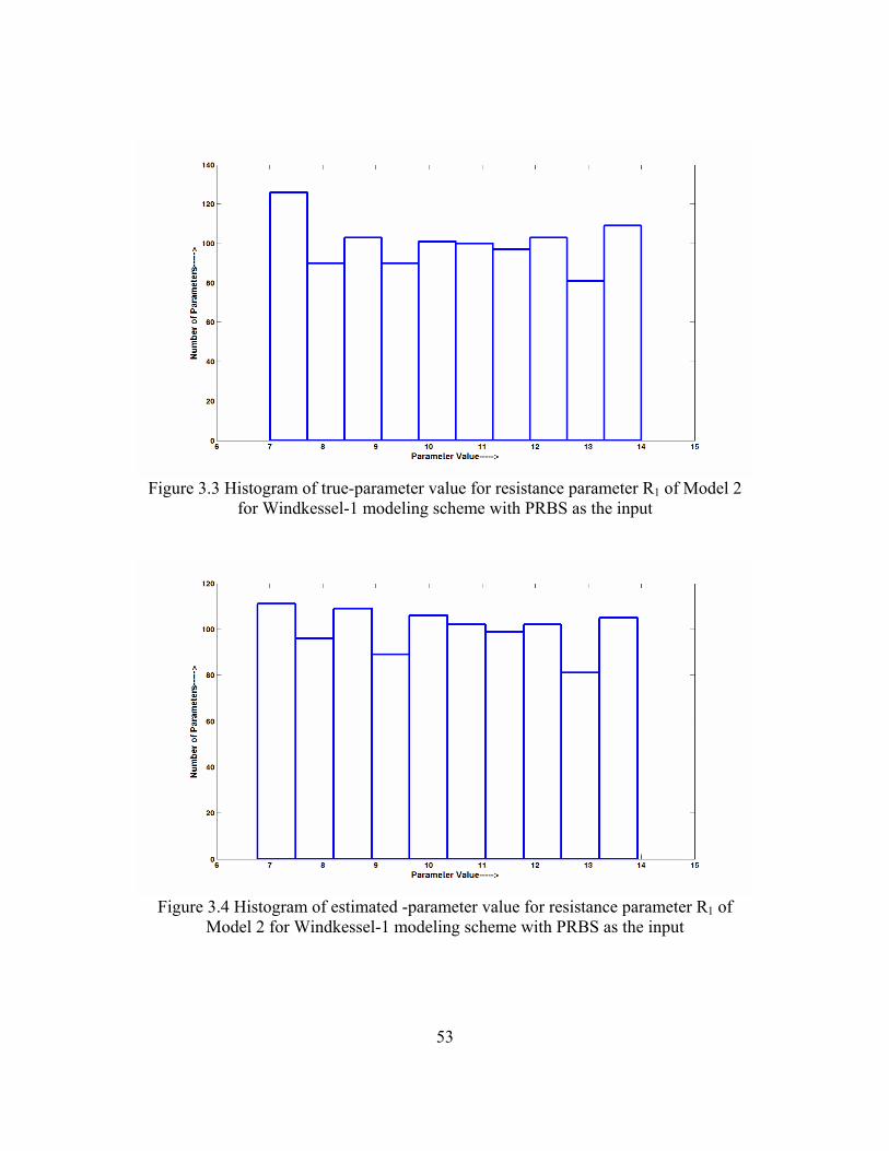
53
Figure 3.3 Histogram of true-parameter value for resistance parameter R1 of Model 2
for Windkessel-1 modeling scheme with PRBS as the input
Figure 3.4 Histogram of estimated -parameter value for resistance parameter R1 of
Model 2 for Windkessel-1 modeling scheme with PRBS as the input

54
Table 3.7 Average values of true-parameters (Ma) and estimated parameters (Me) of Model 3 for Windkessel-1 modeling scheme with PRBS as the input
R1 R2 C1 C2 L1
Average Ma 10.4340 5.5388 3.0050 6.9854 4.5769
STD Ma 2.0706 1.4263 1.1534 1.7559 1.4880
Average Me 31.4310 5.6463 1.6536 6.7841 4.8131
STD Me 46.4680 1.5108 1.1092 1.7332 1.5285
Figure 3.5 Histogram of true-parameter value for resistance parameter R1 of Model 3
for Windkessel-1 modeling scheme with PRBS as the input

55
Figure 3.6 Histogram of estimated -parameter value for resistance parameter R1 of
Model 3 for Windkessel-1 modeling scheme with PRBS as the input
Table 3.8 Average values of true-parameters (Ma) and estimated parameters (Me) of Model 4 for Windkessel-1 modeling scheme with PRBS as the input
R1 R2 C1 C2 L1
Average Ma 10.4340 5.5388 3.0050 6.9854 4.5769
STD Ma 2.0706 1.4263 1.1534 1.7559 1.4880
Average Me 10.3180 4.0332 3.2317 6.7029 4.6186
STD Me 2.0715 0.78857 1.1464 1.7269 1.3515

56
Figure 3.7 Histogram of true-parameter value for resistance parameter R1 of Model 4
for Windkessel-1 modeling scheme with PRBS as the input
Figure 3.8 Histogram of estimated -parameter value for resistance parameter R1 of
Model 4 for Windkessel-1 modeling scheme with PRBS as the input
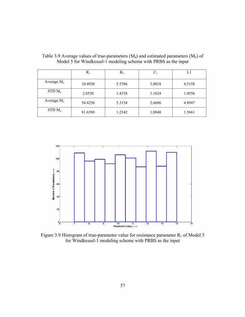
57
Table 3.9 Average values of true-parameters (Ma) and estimated parameters (Me) of Model 5 for Windkessel-1 modeling scheme with PRBS as the input
R1 R2 C1 L1
Average Ma 10.4930 5.5396 3.0018 4.5158
STD Ma 2.0558 1.4338 1.1624 1.4556
Average Me 54.4250 5.3154 2.6686 4.8947
STD Me 81.6580 1.2342 1.0848 1.5661
Figure 3.9 Histogram of true-parameter value for resistance parameter R1 of Model 5
for Windkessel-1 modeling scheme with PRBS as the input

58
Figure 3.10 Histogram of estimated -parameter value for resistance parameter R1 of
Model 5 for Windkessel-1 modeling scheme with PRBS as the input
Table 3.10 Average MSE values for five Windkessel models for Windkessel-1 modeling scheme with PRBS input
Model 1 Model 2 Model 3 Model 4 Model 5
Average MSE 4.5558E-07 1.1422E-06 5.5E-03 3.2178E-006 1.7E-03
STD 8.3469E-07 1.6167E-06 2.91E-02 1.3678E-005 1.5E-03
3.1.2.2 Results for Windkessel-1 Modeling Scheme with MABP Input
This section presents the average MSE values (Table 3.16), true-parameters (Ma)
and estimated-parameters (Me) (Table 3.11 through Table 3.15) of 1000 trials Monte-
Carlo simulation for Windkessel-1 modeling scheme with first 1.5 minute section of the
6 minute MABP (SNI) as the input, for each of the five Windkessel models. Histograms
(Figure 3.11 through Figure 3.20) for true-parameter values and estimated-parameter

59
values for the resistance parameter R1 of each of the five Windkessel models have also
been shown.
Table 3.11 Average values of true-parameters (Ma) and estimated parameters (Me) of Model 1 for Windkessel-1 modeling scheme with MABP as the input
R1 R2 C1
Average Ma 10.5070 5.5285 2.9799
STD Ma 2.0503 1.4220 1.1811
Average Me 10.8330 5.8900 3.2253
STD Me 2.2065 1.8608 1.2817
Figure 3.11 Histogram of true-parameter value for resistance parameter R1 of Model 1
for Windkessel-1 modeling scheme with MABP as the input

60
Figure 3.12 Histogram of estimated -parameter value for resistance parameter R1 of
Model 1 for Windkessel-1 modeling scheme with MABP as the input
Table 3.12 Average values of true-parameters (Ma) and estimated parameters (Me) of Model 2 for Windkessel-1 modeling scheme with MABP as the input
R1 R2 C1 R3 C2
Average Ma 10.4960 5.5047 3.0135 7.0022 4.4622
STD Ma 1.9900 1.4459 1.1878 1.7104 1.4511
Average Me 10.8810 5.7555 3.0349 9.3987 4.7755
STD Me 2.3345 1.9705 1.4158 1.5097 1.3901
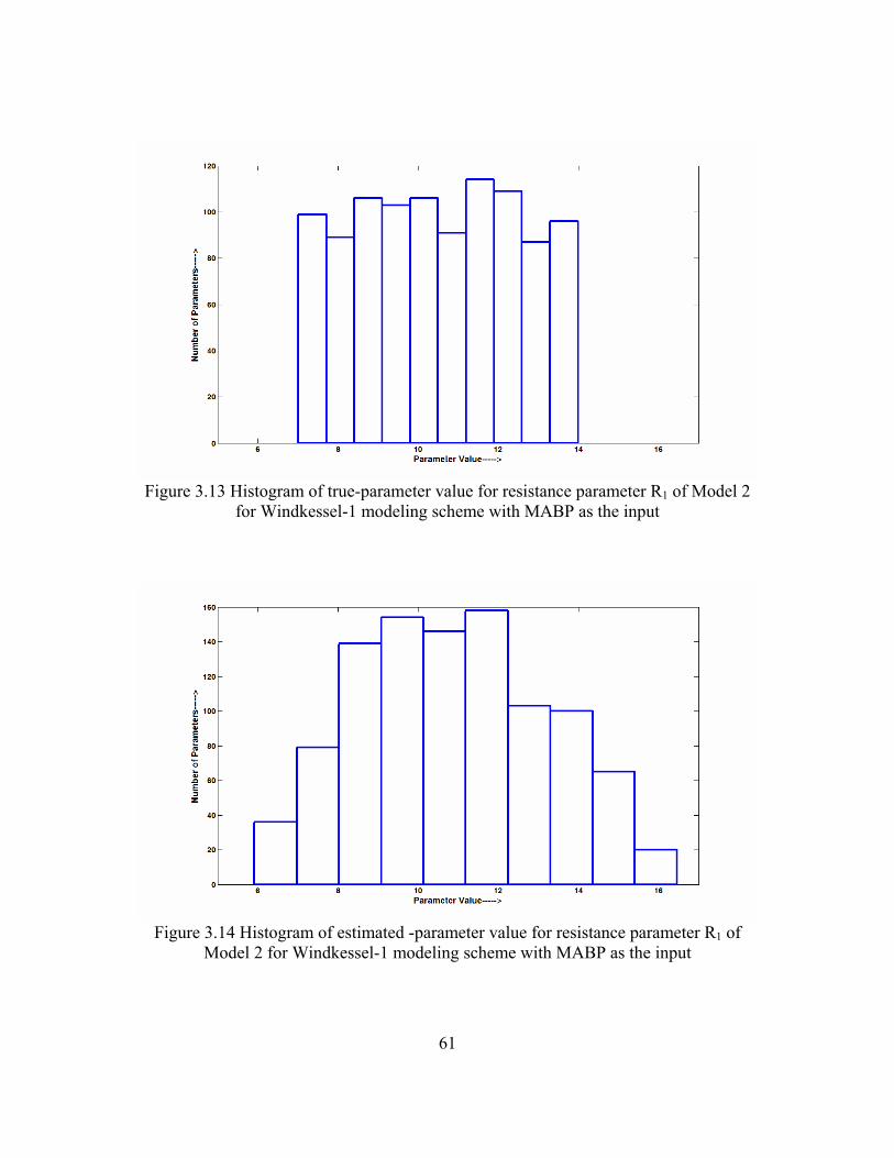
61
Figure 3.13 Histogram of true-parameter value for resistance parameter R1 of Model 2
for Windkessel-1 modeling scheme with MABP as the input
Figure 3.14 Histogram of estimated -parameter value for resistance parameter R1 of
Model 2 for Windkessel-1 modeling scheme with MABP as the input

62
Table 3.13 Average values of true-parameters (Ma) and estimated parameters (Me) of Model 3 for Windkessel-1 modeling scheme with MABP as the input
R1 R2 C1 C2 L1
Average Ma 10.4960 5.5047 3.0135 7.0022 4.4622
STD Ma 1.9900 1.4459 1.1878 1.7104 1.4511
Average Me 3.8924 4.1657 1.2789 7.7019 4.0221
STD Me 11.7690 1.3747 0.9050 1.8541 1.2931
Figure 3.15 Histogram of true-parameter value for resistance parameter R1 of Model 3
for Windkessel-1 modeling scheme with MABP as the input

63
Figure 3.16 Histogram of estimated -parameter value for resistance parameter R1 of
Model 3 for Windkessel-1 modeling scheme with MABP as the input
Table 3.14 Average values of true-parameters (Ma) and estimated parameters (Me) of Model 4 for Windkessel-1 modeling scheme with MABP as the input
R1 R2 C1 C2 L1
Average Ma 10.4960 5.5047 3.0135 7.0022 4.4622
STD Ma 1.9900 1.4459 1.1878 1.7104 1.4511
Average Me 10.7200 4.8132 3.5650 5.9863 3.8964
STD Me 2.3150 2.0204 1.3925 2.1684 1.7830

64
Figure 3.17 Histogram of true-parameter value for resistance parameter R1 of Model 4
for Windkessel-1 modeling scheme with MABP as the input
Figure 3.18 Histogram of estimated -parameter value for resistance parameter R1 of
Model 4 for Windkessel-1 modeling scheme with MABP as the input
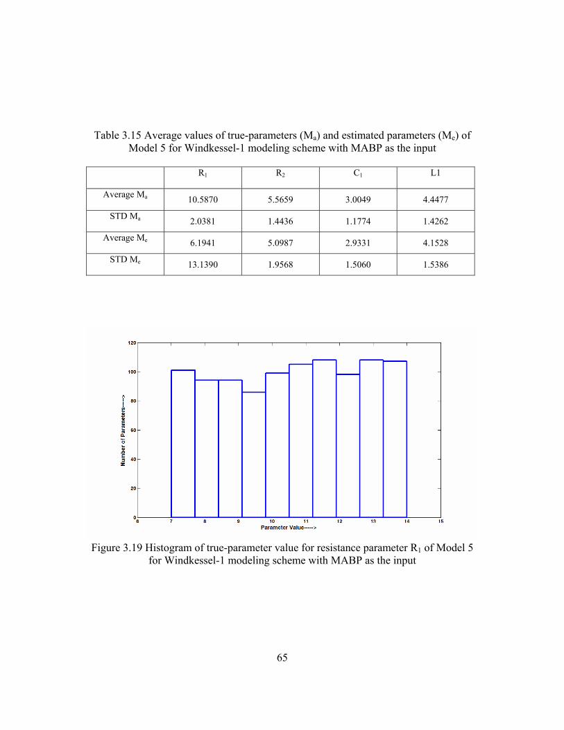
65
Table 3.15 Average values of true-parameters (Ma) and estimated parameters (Me) of Model 5 for Windkessel-1 modeling scheme with MABP as the input
R1 R2 C1 L1
Average Ma 10.5870 5.5659 3.0049 4.4477
STD Ma 2.0381 1.4436 1.1774 1.4262
Average Me 6.1941 5.0987 2.9331 4.1528
STD Me 13.1390 1.9568 1.5060 1.5386
Figure 3.19 Histogram of true-parameter value for resistance parameter R1 of Model 5
for Windkessel-1 modeling scheme with MABP as the input

66
Figure 3.20 Histogram of estimated -parameter value for resistance parameter R1 of
Model 5 for Windkessel-1 modeling scheme with MABP as the input
Table 3.16 Average MSE values for five Windkessel models for Windkessel-1 modeling scheme with MABP input
Model 1 Model 2 Model 3 Model 4 Model 5
Average MSE 1.6983E-06 2.4799E-06 6.03E-02 9.1161E-06 3.95E-02
STD 2.9331E-06 3.5338E-06 2.494E-01 2.2350E-05 1.137E-01
3.1.2.3 Results for Windkessel-2 Modeling Scheme with PRBS Input
This section presents the average MSE values (Table 3.22), true-parameters (Ma)
and estimated-parameters (Me) (Table 3.17 through Table 3.21) of 1000 trials Monte-
Carlo simulation for Windkessel-2 modeling scheme with PRBS as the input, for each
of the five Windkessel models. Histograms (Figure 3.21 through Figure 3.30) for true-
parameter values and estimated-parameter values for the resistance parameter R1 of
each of the five Windkessel models have also been shown.

67
Table 3.17 Average values of true-parameters (Ma) and estimated parameters (Me) of Model 1 for Windkessel-2 modeling scheme with PRBS as the input
R1 R2 C1
Average Ma 10.4230 5.5639 3.0562
STD Ma 2.0503 1.4206 1.1531
Average Me 10.4230 5.2845 3.0761
STD Me 2.0497 1.5010 1.1707
Figure 3.21 Histogram of true-parameter value for resistance parameter R1 of Model 1
for Windkessel-2 modeling scheme with PRBS as the input

68
Figure 3.22 Histogram of estimated -parameter value for resistance parameter R1 of
Model 1 for Windkessel-2 modeling scheme with PRBS as the input
Table 3.18 Average values of true-parameters (Ma) and estimated parameters (Me) of Model 2 for Windkessel-2 modeling scheme with PRBS as the input
R1 R2 C1 R3 C2
Average Ma 10.4340 5.5388 3.0050 6.9854 4.5769
STD Ma 2.0706 1.4263 1.1534 1.7559 1.4880
Average Me 10.4340 4.8745 2.6755 9.6261 4.8651
STD Me 2.0702 1.1828 1.0138 1.2782 0.9148

69
Figure 3.23 Histogram of true-parameter value for resistance parameter R1 of Model 2
for Windkessel-2 modeling scheme with PRBS as the input
Figure 3.24 Histogram of estimated -parameter value for resistance parameter R1 of
Model 2 for Windkessel-2 modeling scheme with PRBS as the input

70
Table 3.19 Average values of true-parameters (Ma) and estimated parameters (Me) of Model 3 for Windkessel-2 modeling scheme with PRBS as the input
R1 R2 C1 C2 L1
Average Ma 10.4340 5.5388 3.0050 6.9854 4.5769
STD Ma 2.0706 1.4263 1.1534 1.7559 1.4880
Average Me 10.4940 5.4479 3.0371 6.9683 4.6976
STD Me 2.1013 1.4639 1.2332 1.7779 1.4910
Figure 3.25 Histogram of true-parameter value for resistance parameter R1 of Model 3
for Windkessel-2 modeling scheme with PRBS as the input

71
Figure 3.26 Histogram of estimated -parameter value for resistance parameter R1 of
Model 3 for Windkessel-2 modeling scheme with PRBS as the input
Table 3.20 Average values of true-parameters (Ma) and estimated parameters (Me) of Model 4 for Windkessel-2 modeling scheme with PRBS as the input
R1 R2 C1 C2 L1
Average Ma 10.4340 5.5388 3.0050 6.9854 4.5769
STD Ma 2.0706 1.4263 1.1534 1.7559 1.4880
Average Me 10.4450 7.6277 3.3873 7.1113 4.0696
STD Me 2.0720 0.75853 1.2572 1.8975 1.4601

72
Figure 3.27 Histogram of true-parameter value for resistance parameter R1 of Model 4
for Windkessel-2 modeling scheme with PRBS as the input
Figure 3.28 Histogram of estimated -parameter value for resistance parameter R1 of
Model 4 for Windkessel-2 modeling scheme with PRBS as the input

73
Table 3.21 Average values of true-parameters (Ma) and estimated parameters (Me) of Model 5 for Windkessel-2 modeling scheme with PRBS as the input
R1 R2 C1 L1
Average Ma 10.4930 5.5396 3.0018 4.5158
STD Ma 2.0558 1.4338 1.1624 1.4556
Average Me 10.4930 5.5396 3.0018 4.5158
STD Me 2.0559 1.4338 1.1624 1.4556
Figure 3.29 Histogram of true-parameter value for resistance parameter R1 of Model 5
for Windkessel-2 modeling scheme with PRBS as the input

74
Figure 3.30 Histogram of estimated -parameter value for resistance parameter R1 of
Model 5 for Windkessel-2 modeling scheme with PRBS as the input
Table 3.22 Average MSE values for five Windkessel models for Windkessel-2 modeling scheme with PRBS input
Model 1 Model 2 Model 3 Model 4 Model 5
Average MSE 2.1995E-08 3.1807E-08 4.6E-03 4.6159E-06 7.0492E-11
STD 1.0012E-07 1.7981E-07 2.92E-02 1.4494E-05 5.9846E-10
3.1.2.4 Results for Windkessel-2 Modeling Scheme with MABP Input
This section presents the average MSE values (Table 3.28), true-parameters (Ma)
and estimated-parameters (Me) (Table 3.23 through Table 3.27) of 1000 trials Monte-
Carlo simulation for Windkessel-2 modeling scheme with first 1.5 minute section of the
6 minute MABP (SNI) as the input, for each of the five Windkessel models. Histograms
(Figure 3.31 through Figure 3.40) for true-parameter values and estimated-parameter

75
values for the resistance parameter R1 of each of the five Windkessel models have also
been shown.
Table 3.23 Average values of true-parameters (Ma) and estimated parameters (Me) of Model 1 for Windkessel-2 modeling scheme with MABP as the input
R1 R2 C1
Average Ma 10.5070 5.5285 2.9799
STD Ma 2.0503 1.4220 1.1811
Average Me 10.5160 5.5097 3.0334
STD Me 2.0557 1.6138 1.2273
Figure 3.31 Histogram of true-parameter value for resistance parameter R1 of Model 1
for Windkessel-2 modeling scheme with MABP as the input

76
Figure 3.32 Histogram of estimated -parameter value for resistance parameter R1 of
Model 1 for Windkessel-2 modeling scheme with MABP as the input
Table 3.24 Average values of true-parameters (Ma) and estimated parameters (Me) of Model 2 for Windkessel-2 modeling scheme with MABP as the input
R1 R2 C1 R3 C2
Average Ma 10.4960 5.5047 3.0135 7.0022 4.4622
STD Ma 1.9900 1.4459 1.1878 1.7104 1.4511
Average Me 10.4990 5.4583 2.6018 9.2680 5.1708
STD Me 1.9917 1.4876 1.0598 1.6538 0.97631
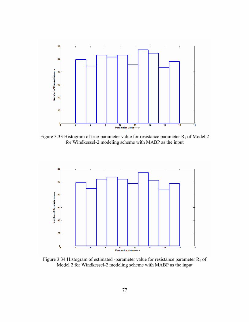
77
Figure 3.33 Histogram of true-parameter value for resistance parameter R1 of Model 2
for Windkessel-2 modeling scheme with MABP as the input
Figure 3.34 Histogram of estimated -parameter value for resistance parameter R1 of
Model 2 for Windkessel-2 modeling scheme with MABP as the input
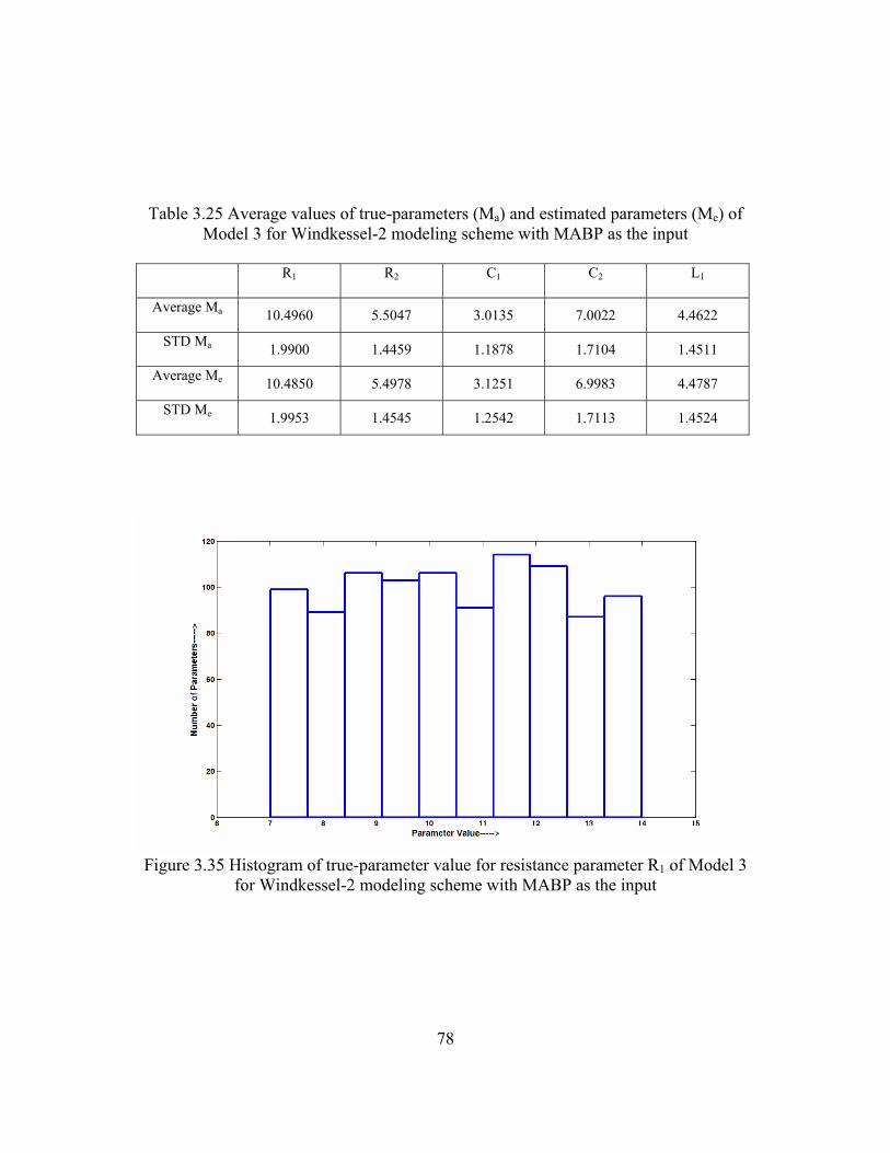
78
Table 3.25 Average values of true-parameters (Ma) and estimated parameters (Me) of Model 3 for Windkessel-2 modeling scheme with MABP as the input
R1 R2 C1 C2 L1
Average Ma 10.4960 5.5047 3.0135 7.0022 4.4622
STD Ma 1.9900 1.4459 1.1878 1.7104 1.4511
Average Me 10.4850 5.4978 3.1251 6.9983 4.4787
STD Me 1.9953 1.4545 1.2542 1.7113 1.4524
Figure 3.35 Histogram of true-parameter value for resistance parameter R1 of Model 3
for Windkessel-2 modeling scheme with MABP as the input

79
Figure 3.36 Histogram of estimated -parameter value for resistance parameter R1 of
Model 3 for Windkessel-2 modeling scheme with MABP as the input
Table 3.26 Average values of true-parameters (Ma) and estimated parameters (Me) of Model 4 for Windkessel-2 modeling scheme with MABP as the input
R1 R2 C1 C2 L1
Average Ma 10.4960 5.5047 3.0135 7.0022 4.4622
STD Ma 1.9900 1.4459 1.1878 1.7104 1.4511
Average Me 10.7350 7.4248 3.7271 7.4639 4.1468
STD Me 2.0262 1.1877 1.2832 2.0851 1.6313

80
Figure 3.37 Histogram of true-parameter value for resistance parameter R1 of Model 4
for Windkessel-2 modeling scheme with MABP as the input
Figure 3.38 Histogram of estimated -parameter value for resistance parameter R1 of
Model 4 for Windkessel-2 modeling scheme with MABP as the input

81
Table 3.27 Average values of true-parameters (Ma) and estimated parameters (Me) of Model 5 for Windkessel-2 modeling scheme with MABP as the input
R1 R2 C1 L1
Average Ma 10.5870 5.5659 3.0049 4.4477
STD Ma 2.0381 1.4436 1.1774 1.4262
Average Me 10.5870 5.5659 3.0049 4.4477
STD Me 2.0387 1.4437 1.1774 1.4262
Figure 3.39 Histogram of true-parameter value for resistance parameter R1 of Model 5
for Windkessel-2 modeling scheme with MABP as the input

82
Figure 3.40 Histogram of estimated-parameter value for resistance parameter R1 of
Model 5 for Windkessel-2 modeling scheme with MABP as the input
Table 3.28 Average MSE values for five Windkessel models for Windkessel-2 modeling scheme with MABP input
Model 1 Model 2 Model 3 Model 4 Model 5
Average MSE 1.2628E-08 2.6668E-08 8.2433E-04 6.5998E-06 2.5043E-10
STD 3.8493E-08 6.7055E-08 1.33E-02 1.6543E-05 5.1541E-09
3.2 Modeling Results for MABP and CBFV Data
This section presents the results of applying various linear, lumped parameter
models and modeling methodologies, discussed in section 2.2, to MABP and CBFV
data of all the 10 subjects for the four types of data conditions (SNI, SI, VNI, and VI).

83
3.2.1 MSE and Parameter Value Results
This section presents MSE values and average parameter values for 10 subjects
using the ARX models (ARX-1 and ARX-2 modeling schemes described in section
2.2.1) and the five Windkessel models (Windkessel-1, Windkessel-2, and Windkessel-3
modeling schemes described in section 2.2.3).
Appendix B presents the results for the comparisons based on t-tests (Pval) for
the MSE values of 10 subjects for four data conditions, between ARX-2, Windkessel-1,
Windkessel-2 and Windkessel-3 modeling schemes. The statistical level of significance
for the t-tests was selected to be 0.05. For Windkessel modeling schemes, the
comparison was done between MSE value results with different schemes for a given
model. These comparisons were done for all the five Windkessel models. For
comparing ARX-2 with Windkessel-1 and Windkessel-2 modeling schemes, models
with the similar order were considered.
3.2.1.1 Results for ARX Models
Table 3.29 shows the MSE values of 10 subjects for four conditions of data with
ARX-1 modeling scheme. Table 3.30 shows the average numerator (m) and
denominator (n) model orders for the same. Table 3.31, Table 3.33 and Table 3.35 show
the MSE values of 10 subjects for four conditions of data with ARX-2 modeling
scheme, for the 1st, 2nd, and 3rd order models respectively. The average model
parameters (as per the model structure in Equation 1.4) for each of the four data

84
conditions are shown in the Table 3.32, Table 3.34 and Table 3.36, for the 1st, 2nd, and
3rd order models respectively with ARX-2 modeling scheme.
Table 3.29 MSE values for four data conditions of 10 subjects
with ARX-1 modeling scheme
Subject No. SNI SI VNI VI
1 0.0125 0.0232 0.0140 0.0277
2 0.0404 0.0331 0.0248 0.0121
3 0.0190 0.0399 0.0093 0.0462
4 0.0237 0.0290 0.0131 0.0386
5 0.0280 0.0482 0.0287 0.1145
6 0.0217 0.0397 0.0502 0.0297
7 0.0251 0.0245 0.0184 0.0436
8 0.0214 0.0506 0.0126 0.0190
9 0.0155 0.0264 0.0176 2.8671
10 0.0208 0.0266 0.0146 0.0143
Average 0.0228 0.0341 0.0203 0.3213
STD 0.0076 0.0099 0.0120 0.8950
Table 3.30 Numerator (m) and denominator (n) model orders for four data conditions of 10 subjects with ARX-1 modeling scheme
SNI SI VNI VI
Subject No. m n m m n n m n
1 4 4 10 10 2 2 1 1
2 8 8 10 10 7 7 10 10
3 8 8 10 10 9 9 9 9
4 9 9 1 1 10 10 2 2
5 10 10 2 2 2 2 6 6

85
Table 3.30 Continued. 6 10 10 4 4 2 2 6 6
7 8 8 10 10 10 10 2 2
8 9 9 6 6 9 9 2 2
9 10 10 10 10 2 2 1 1
10 9 9 3 3 6 6 3 3
Average 8.5 8.5 6.6 6.6 5.9 5.9 4.2 4.2
STD 1.8 1.8 3.8 3.8 3.6 3.6 3.3 3.3
Table 3.31 MSE values for four data conditions of 10 subjects with ARX-2 modeling scheme for 1st order model (m=n=1)
Subject No. SNI SI VNI VI
1 0.0139 0.0262 0.0294 0.0277
2 0.0503 0.0535 0.0295 0.0237
3 0.0295 0.0476 0.0123 0.7397
4 0.0541 0.0290 0.0215 0.0464
5 0.0536 0.0554 0.0832 0.8201
6 0.0246 0.0504 0.0610 0.0507
7 0.0501 0.0274 0.0244 0.0488
8 0.0401 0.0522 0.0416 0.0215
9 0.0311 0.0376 0.0206 2.8671
10 0.0362 0.0332 0.0200 0.0149
Average 0.0383 0.0412 0.0344 0.4661
STD 0.0137 0.0117 0.0220 0.8992

86
Table 3.32 Average parameter values for four data conditions of 10 subjects with ARX-2 modeling scheme for 1st order model (m=n=1)
a1 b0 b1
SNI Average -0.9424 0.6228 -0.6809
SNI STD 0.0408 0.2926 0.2845
SI Average -0.9504 0.41563 -0.4430
SI STD 0.0195 0.3341 0.3087
VNI Average -0.9405 0.5385 -0.5804
VNI STD 0.0393 0.0841 0.0768
VI Average -0.9665 0.2961 -0.3676
VI STD 0.0484 0.2605 0.2666
Table 3.33 MSE values for four data conditions of 10 subjects with ARX-2 modeling scheme for 2nd order model (m=n=2)
Subject No. SNI SI VNI VI
1 0.0162 0.0251 0.0140 0.0277
2 0.0426 0.0394 0.0251 0.0169
3 0.0211 0.0489 0.0111 0.0526
4 0.0292 0.0298 0.0164 0.0390
5 0.0283 0.0482 0.0287 0.1535
6 0.0257 0.0398 0.0502 0.0463
7 0.0324 0.0261 0.0253 0.0448
8 0.0255 0.0548 0.0173 0.0209
9 0.0267 0.0290 0.0176 95.3820
10 0.0259 0.0285 0.0149 0.0143
Average 0.0274 0.0370 0.0221 9.5798
STD 0.0069 0.0108 0.0114 30.1478

87
Table 3.34 Average parameter values for four data conditions of 10 subjects with ARX-2 modeling scheme for 2nd order model (m=n=2)
a1 a2 b0 b1 b2
SNI Average -1.6204 0.6743 0.6679 -1.1657 -1.6204
SNI STD 0.1045 0.0907 0.2595 0.4542 0.2126
SI Average -1.4478 0.5283 0.3976 -0.5908 -1.4478
SI STD 0.1050 0.1154 0.3417 0.5411 0.2324
VNI Average -1.4289 0.4990 0.5183 -0.7849 -1.4289
VNI STD 0.1992 0.1678 0.1237 0.2339 0.1667
VI Average -1.2411 0.2845 0.1340 -0.0397 -1.2411
VI STD 0.3203 0.3273 0.3606 0.7340 0.4220
Table 3.35 MSE values for four data conditions of 10 subjects with ARX-2 modeling scheme for 3rd order model (m=n=3)
Subject No. SNI SI VNI VI
1 0.0154 0.0256 0.0245 0.0326
2 0.0436 0.0469 0.0253 0.0150
3 0.0210 0.0470 0.0099 0.0593
4 0.0282 0.0304 0.0178 0.0483
5 0.0285 0.0496 0.0481 0.2245
6 0.0238 0.0420 0.0564 0.0407
7 0.0332 0.0281 0.0199 0.0553
8 0.0299 0.0522 0.0169 0.0228
9 0.0397 0.0331 0.0217 1579.4000
10 0.0259 0.0266 0.0176 0.0143
Average 0.0289 0.0381 0.0258 157.9913
STD 0.0084 0.0104 0.0147 499.4321
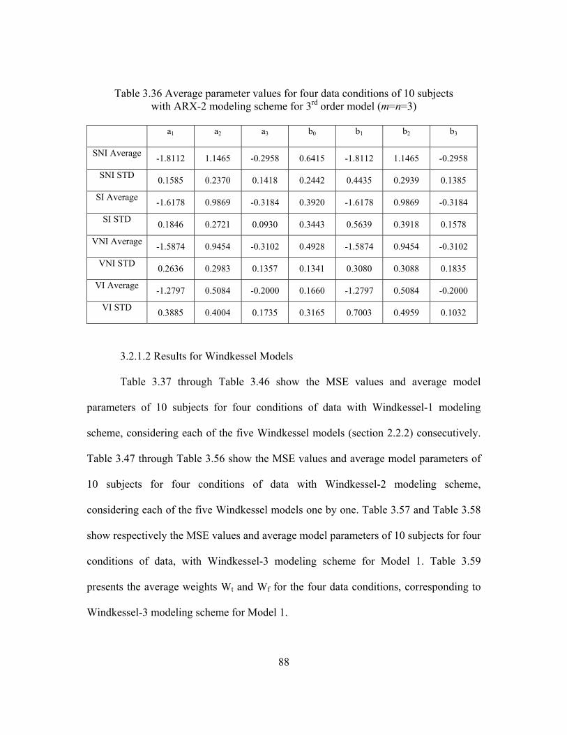
88
Table 3.36 Average parameter values for four data conditions of 10 subjects with ARX-2 modeling scheme for 3rd order model (m=n=3)
a1 a2 a3 b0 b1 b2 b3
SNI Average -1.8112 1.1465 -0.2958 0.6415 -1.8112 1.1465 -0.2958
SNI STD 0.1585 0.2370 0.1418 0.2442 0.4435 0.2939 0.1385
SI Average -1.6178 0.9869 -0.3184 0.3920 -1.6178 0.9869 -0.3184
SI STD 0.1846 0.2721 0.0930 0.3443 0.5639 0.3918 0.1578
VNI Average -1.5874 0.9454 -0.3102 0.4928 -1.5874 0.9454 -0.3102
VNI STD 0.2636 0.2983 0.1357 0.1341 0.3080 0.3088 0.1835
VI Average -1.2797 0.5084 -0.2000 0.1660 -1.2797 0.5084 -0.2000
VI STD 0.3885 0.4004 0.1735 0.3165 0.7003 0.4959 0.1032
3.2.1.2 Results for Windkessel Models
Table 3.37 through Table 3.46 show the MSE values and average model
parameters of 10 subjects for four conditions of data with Windkessel-1 modeling
scheme, considering each of the five Windkessel models (section 2.2.2) consecutively.
Table 3.47 through Table 3.56 show the MSE values and average model parameters of
10 subjects for four conditions of data with Windkessel-2 modeling scheme,
considering each of the five Windkessel models one by one. Table 3.57 and Table 3.58
show respectively the MSE values and average model parameters of 10 subjects for four
conditions of data, with Windkessel-3 modeling scheme for Model 1. Table 3.59
presents the average weights Wt and Wf for the four data conditions, corresponding to
Windkessel-3 modeling scheme for Model 1.

89
Table 3.37 MSE values for four data conditions of 10 subjects with Windkessel-1 modeling scheme for Model 1
Subject No. SNI SI VNI VI
1 0.0260 0.0277 0.0191 0.0238
2 0.0587 0.0546 0.0270 0.1504
3 0.0368 0.0498 0.0179 0.0201
4 0.0298 0.0351 0.0254 0.0485
5 0.0771 0.0530 0.0199 0.0363
6 0.0382 0.0372 0.0735 0.0169
7 0.0290 0.0321 0.0428 0.0287
8 0.0533 0.0819 0.0250 0.0341
9 0.0242 0.0263 0.0227 0.0385
10 0.0288 0.0279 0.0129 0.0381
Average 0.0402 0.0426 0.0286 0.0435
STD 0.0174 0.0175 0.0177 0.0387
Table 3.38 Average parameter values for four data conditions of 10 subjects with Windkessel-1 modeling scheme for Model 1
R1 R2 C1
SNI Average 1.5329 8.8824 28.3617
SNI STD 0.7145 6.6301 23.2065
SI Average 1.9924 9.7894 32.5481
SI STD 1.4844 6.2837 23.4758
VNI Average 2.3760 8.1754 16.2462
VNI STD 2.0864 5.7005 18.0469
VI Average 1.3973 9.6666 13.1472
VI STD 1.9086 8.7017 15.0612

90
Table 3.39 MSE values for four data conditions of 10 subjects with Windkessel-1 modeling scheme for Model 2
Subject No. SNI SI VNI VI
1 0.0244 0.0273 0.0189 0.0228
2 0.0593 0.0531 0.0269 0.1510
3 0.0362 0.0477 0.0161 0.0147
4 0.0289 0.0355 0.0269 0.0433
5 0.0761 0.0576 0.0254 0.0336
6 0.0376 0.0370 0.0731 0.0165
7 0.0300 0.0318 0.0463 0.0278
8 0.0520 0.0957 0.0268 0.0338
9 0.0261 0.0261 0.0224 0.0725
10 0.0378 0.0266 0.0198 0.0303
Average 0.0408 0.0438 0.0303 0.0446
STD 0.0167 0.0214 0.0172 0.0408
Table 3.40 Average parameter values for four data conditions of 10 subjects with Windkessel-1 modeling scheme for Model 2
R1 R2 C1 R3 C2
SNI Average 1.5329 26.2551 35.7744 26.2550 35.7744
SNI STD 0.7145 2.7918 22.9332 2.7919 22.9332
SI Average 1.9924 26.2119 27.7462 26.2115 27.7461
SI STD 1.4844 4.1990 21.5947 4.1991 21.5948
VNI Average 2.3760 25.0278 17.4914 25.0278 17.4914
VNI STD 2.0864 0.3238 15.3908 0.3238 15.3908
VI Average 1.3973 27.4183 19.9709 27.4183 19.9773
VI STD 1.9086 4.8475 15.9619 4.8475 15.9551

91
Table 3.41 MSE values for four data conditions of 10 subjects with Windkessel-1 modeling scheme for Model 3
Subject No. SNI SI VNI VI
1 0.0684 0.0264 0.0176 0.0306
2 0.0492 0.0515 0.0279 0.1388
3 0.0388 0.0507 0.0189 0.0176
4 0.0272 0.0301 0.0269 0.0508
5 0.0791 0.0640 0.0261 0.0284
6 0.0423 0.0376 0.1761 0.0173
7 0.0289 0.0371 0.0451 0.0307
8 0.0509 0.0899 0.0243 0.0273
9 0.0234 0.0253 0.0248 0.0477
10 0.0266 0.0289 0.0191 0.0662
Average 0.0435 0.0442 0.0407 0.0455
STD 0.0188 0.0205 0.0482 0.0362
Table 3.42 Average parameter values for four data conditions of 10 subjects with Windkessel-1 modeling scheme for Model 3
R1 R2 C1 C2 L1
SNI Average 1.5329 20.3869 29.7503 4.7524 19.6246
SNI STD 0.7145 13.6190 17.6996 10.9252 33.8786
SI Average 1.9924 16.4572 27.1882 18.4241 30.8701
SI STD 1.4844 16.4845 19.8806 38.4956 47.5156
VNI Average 2.3760 25.9372 20.1745 10.0448 12.4469
VNI STD 2.0864 19.4526 15.8554 31.6071 31.1373
VI Average 1.3973 19.3522 20.4882 17.6723 24.5257
VI STD 1.9086 13.3254 14.9148 35.9070 39.0916

92
Table 3.43 MSE values for four data conditions of 10 subjects with Windkessel-1 modeling scheme for Model 4
Subject No. SNI SI VNI VI
1 0.0646 0.0281 0.0188 0.0337
2 0.0601 0.0488 0.0267 0.1560
3 0.0368 0.0497 0.0116 0.0144
4 0.0251 0.0352 0.0268 0.0486
5 0.0769 0.0651 0.0187 0.0307
6 0.0371 0.0371 0.0788 0.0166
7 0.0297 0.0317 0.0485 0.0407
8 0.0535 0.0991 0.0262 0.0343
9 0.0246 0.0265 0.0231 0.0766
10 0.0574 0.0273 0.0185 0.0397
Average 0.0466 0.0449 0.0298 0.0491
STD 0.0183 0.0227 0.0198 0.0414
Table 3.44 Average parameter values for four data conditions of 10 subjects with Windkessel-1 modeling scheme for Model 4
R1 R2 C1 C2 L1
SNI Average 1.5329 25.3912 33.1921 26.1667 24.0506
SNI STD 0.7145 2.3732 18.6805 8.3929 16.7926
SI Average 1.9924 26.9083 27.5887 30.5677 24.1092
SI STD 1.4844 3.3342 16.9141 10.3460 6.7627
VNI Average 2.3760 21.5490 14.9707 35.7082 30.8593
VNI STD 2.0864 4.7502 11.8517 15.4627 13.9224
VI Average 1.3973 22.8528 19.5813 23.0911 32.8060
VI STD 1.9086 8.9954 18.7893 14.2796 25.4029

93
Table 3.45 MSE values for four data conditions of 10 subjects with Windkessel-1 modeling scheme for Model 5
Subject No. SNI SI VNI VI
1 0.0251 0.0267 0.0219 0.0230
2 0.0587 0.0536 0.0314 0.1503
3 0.0283 0.0508 0.0096 0.0146
4 0.0268 0.0346 0.0252 0.0341
5 0.0354 0.0632 0.0218 0.0356
6 0.0290 0.0384 0.0782 0.0166
7 0.0285 0.0264 0.0458 0.0281
8 0.0282 0.0818 0.0146 0.0322
9 0.0170 0.0290 0.0218 0.0712
10 0.0371 0.0242 0.0213 0.0315
Average 0.0314 0.0429 0.0292 0.0437
STD 0.0110 0.0191 0.0198 0.0406
Table 3.46 Average parameter values for four data conditions of 10 subjects with Windkessel-1 modeling scheme for Model 5
R1 R2 C1 L1
SNI Average 1.5329 23.6617 8.8275 44.7052
SNI STD 0.7145 0.9367 15.7902 18.2145
SI Average 1.9924 21.5743 12.3457 36.0597
SI STD 1.4844 7.5678 16.7438 15.5624
VNI Average 2.3760 23.3314 7.7868 48.1243
VNI STD 2.0864 2.7300 8.2423 14.4253
VI Average 1.3973 23.6883 6.6599 65.1797
VI STD 1.9086 1.1810 6.4392 27.4140

94
Table 3.47 MSE values for four data conditions of 10 subjects with Windkessel-2 modeling scheme for Model 1
Subject No. SNI SI VNI VI
1 0.0449 0.0242 0.0185 0.0340
2 0.0591 0.0495 0.0270 0.0234
3 0.0359 0.0473 0.0177 0.0199
4 0.0268 0.0312 0.0298 0.0464
5 0.0422 0.0477 0.0175 0.0347
6 0.0370 0.0368 0.0830 0.0352
7 0.0290 0.0282 0.0330 0.0572
8 0.0460 0.0578 0.0226 0.0310
9 0.0193 0.0252 0.0222 0.0773
10 0.0349 0.0274 0.0129 0.0426
Average 0.0375 0.0375 0.0284 0.0402
STD 0.0113 0.0121 0.0202 0.0169
Table 3.48 Average parameter values for four data conditions of 10 subjects with Windkessel-2 modeling scheme for Model 1
R1 R2 C1
SNI Average 8.0161 8.2612 33.0462
SNI STD 10.2749 6.3452 22.3281
SI Average 8.6681 9.7120 32.7543
SI STD 15.4876 6.2425 23.5232
VNI Average 9.1973 8.2614 22.6639
VNI STD 12.0709 6.3383 20.0251
VI Average 22.9406 10.3099 23.5276
VI STD 38.3065 8.2813 23.2020
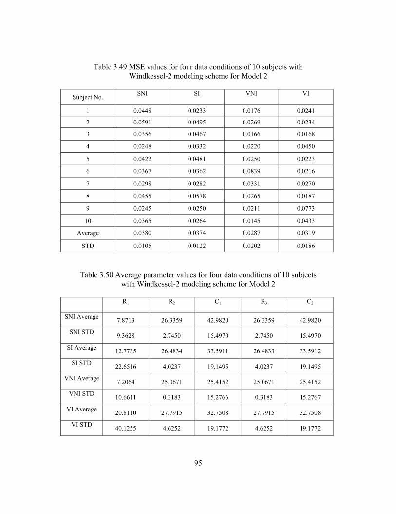
95
Table 3.49 MSE values for four data conditions of 10 subjects with Windkessel-2 modeling scheme for Model 2
Subject No. SNI SI VNI VI
1 0.0448 0.0233 0.0176 0.0241
2 0.0591 0.0495 0.0269 0.0234
3 0.0356 0.0467 0.0166 0.0168
4 0.0248 0.0332 0.0220 0.0450
5 0.0422 0.0481 0.0250 0.0223
6 0.0367 0.0362 0.0839 0.0216
7 0.0298 0.0282 0.0331 0.0270
8 0.0455 0.0578 0.0265 0.0187
9 0.0245 0.0250 0.0211 0.0773
10 0.0365 0.0264 0.0145 0.0433
Average 0.0380 0.0374 0.0287 0.0319
STD 0.0105 0.0122 0.0202 0.0186
Table 3.50 Average parameter values for four data conditions of 10 subjects with Windkessel-2 modeling scheme for Model 2
R1 R2 C1 R3 C2
SNI Average 7.8713 26.3359 42.9820 26.3359 42.9820
SNI STD 9.3628 2.7450 15.4970 2.7450 15.4970
SI Average 12.7735 26.4834 33.5911 26.4833 33.5912
SI STD 22.6516 4.0237 19.1495 4.0237 19.1495
VNI Average 7.2064 25.0671 25.4152 25.0671 25.4152
VNI STD 10.6611 0.3183 15.2766 0.3183 15.2767
VI Average 20.8110 27.7915 32.7508 27.7915 32.7508
VI STD 40.1255 4.6252 19.1772 4.6252 19.1772

96
Table 3.51 MSE values for four data conditions of 10 subjects with Windkessel-2 modeling scheme for Model 3
Subject No. SNI SI VNI VI
1 0.0401 0.0260 0.0173 0.0480
2 0.0540 0.0489 0.0273 0.0226
3 0.0361 0.0477 0.0181 0.0167
4 0.0273 0.0301 0.0206 0.0454
5 0.0481 0.0473 0.0262 0.0340
6 0.0365 0.0375 0.0991 0.0204
7 0.0288 0.0281 0.0291 0.0399
8 0.0335 0.0567 0.0236 0.0272
9 0.0214 0.0257 0.0247 0.0513
10 0.0350 0.0411 0.0133 0.0474
Average 0.0361 0.0389 0.0299 0.0353
STD 0.0097 0.0111 0.0248 0.0128
Table 3.52 Average parameter values for four data conditions of 10 subjects with Windkessel-2 modeling scheme for Model 3
R1 R2 C1 C2 L1
SNI Average 15.8771 20.1355 31.2447 4.1391 21.8415
SNI STD 28.6559 13.9423 15.8133 10.5438 32.7747
SI Average 21.3474 16.5538 29.1594 20.9048 31.1317
SI STD 30.9661 16.4512 16.3215 38.0726 47.5442
VNI Average 8.5425 22.2618 21.0075 11.7651 18.8416
VNI STD 10.2881 14.0492 14.7906 31.4168 34.5104
VI Average 14.0066 18.1953 19.4946 14.2211 19.9405
VI STD 30.3783 12.6804 15.9043 31.8751 31.9251

97
Table 3.53 MSE values for four data conditions of 10 subjects with Windkessel-2 modeling scheme for Model 4
Subject No. SNI SI VNI VI
1 0.0449 0.0250 0.0175 0.0335
2 0.0587 0.0497 0.0267 0.0234
3 0.0358 0.0474 0.0177 0.0152
4 0.0229 0.0317 0.0200 0.0468
5 0.0422 0.0481 0.0160 0.0333
6 0.0367 0.0366 0.0836 0.0385
7 0.0296 0.0281 0.0330 0.0587
8 0.0449 0.0578 0.0251 0.0341
9 0.0210 0.0256 0.0231 0.0773
10 0.0367 0.0269 0.0137 0.0413
Average 0.0373 0.0377 0.0277 0.0402
STD 0.0112 0.0120 0.0205 0.0177
Table 3.54 Average parameter values for four data conditions of 10 subjects with Windkessel-2 modeling scheme for Model 4
R1 R2 C1 C2 L1
SNI Average 7.9718 25.2762 35.0544 26.3504 25.2036
SNI STD 9.6189 2.3398 16.9732 8.2224 15.6754
SI Average 12.6025 26.6225 30.0333 30.2972 23.7685
SI STD 21.7436 3.3404 14.1941 10.4237 7.2445
VNI Average 7.3461 24.2064 24.0120 26.3904 25.4370
VNI STD 10.8016 2.9012 17.1942 12.9344 8.4018
VI Average 38.1045 22.9304 26.8146 22.0406 23.2772
VI STD 43.7974 7.5044 21.7643 8.7158 15.4406

98
Table 3.55 MSE values for four data conditions of 10 subjects with Windkessel-2 modeling scheme for Model 5
Subject No. SNI SI VNI VI
1 0.0688 0.0241 0.0246 0.0165
2 0.0588 0.0483 0.0367 0.0195
3 0.0219 0.0547 0.0071 0.0299
4 0.0292 0.0344 0.0207 0.0292
5 0.0443 0.0471 0.0197 0.0163
6 0.0458 0.0395 0.0852 0.0518
7 0.0282 0.0300 0.0311 0.0273
8 0.0487 0.0580 0.0156 0.0129
9 0.0204 0.0334 0.0149 0.0555
10 0.0363 0.0308 0.0198 0.0471
Average 0.0403 0.0400 0.0275 0.0306
STD 0.0159 0.0114 0.0219 0.0156
Table 3.56 Average parameter values for four data conditions of 10 subjects with Windkessel-2 modeling scheme for Model 5
R1 R2 C1 L1
SNI Average 7.2792 23.8807 15.6092 33.5468
SNI STD 10.6041 0.9630 9.1328 9.0880
SI Average 11.7018 21.4158 17.0747 28.9838
SI STD 16.4643 7.6545 16.2064 13.7019
VNI Average 8.1035 23.3604 12.4817 46.5449
VNI STD 11.8645 1.4264 14.6355 20.7988
VI Average 21.0600 24.2553 17.6818 46.2396
VI STD 34.3533 1.0850 17.4619 22.3397

99
Table 3.57 MSE values for four data conditions of 10 subjects with Windkessel-3 modeling scheme for Model 1
Subject No. SNI SI VNI VI
1 0.0365 0.0239 0.0207 0.0273
2 0.0944 0.0902 0.0526 0.0538
3 0.0521 0.0503 0.0171 0.0211
4 0.0279 0.0302 0.0359 0.0531
5 0.0975 0.0503 0.0282 0.0211
6 0.0526 0.0419 0.0952 0.0416
7 0.0291 0.0298 0.0390 0.0580
8 0.0301 0.0563 0.0231 0.0301
9 0.0222 0.0391 0.0241 0.0720
10 0.0446 0.0270 0.0140 0.0579
Average 0.0487 0.0439 0.0350 0.0436
STD 0.0269 0.0197 0.0241 0.0179
Table 3.58 Average parameter values for four data conditions of 10 subjects with Windkessel-3 modeling scheme for Model 1
R1 R2 C1
SNI Average 1.1567 3.8006 44.2428
SNI STD 0.3219 4.8674 39.8917
SI Average 1.2516 7.9053 52.1906
SI STD 0.6362 11.2822 36.0690
VNI Average 1.1649 10.4179 46.2739
VNI STD 0.3734 14.5268 39.3100
VI Average 0.8747 15.6321 42.9288
VI STD 0.4751 29.9415 36.7434

100
Table 3.59 Average weights (Wt and Wf) for four data conditions of 10 subjects with Windkessel-3 modeling scheme for Model 1
Wt Wf
SNI Average 0.3000 0.7000
SNI STD 0.2981 0.2981
SI Average 0.2500 0.7500
SI STD 0.2014 0.2014
VNI Average 0.2400 0.7600
VNI STD 0.1350 0.1350
VI Average 0.3800 0.6200
VI STD 0.2741 0.2741

101
3.2.2 Graphical Validation Results
This section presents the plots of measured data and model outputs for CBFV as
a function of MABP under various modeling methodologies, discussed in section 2.2.
The frequency responses of the models have also been shown. For comparing
Windkessel-1 and Windkessel-2 methodologies, the corresponding model output plots
and frequency response plots have been shown for the same subject, along with the
measured input (MABP) and output (CBFV) data. Similarly the corresponding ARX-1
and ARX-2 model output plots and frequency response plots have been shown for the
same subject, along with the measured data. For Windkessel modeling schemes, the
comparison was done based on results for the same given model, and models with the
similar order were considered for generating the corresponding ARX-2 plots. The plots
for Windkessel-3 modeling scheme have been shown separately.
Since the results of these studies are numerous (a total of 240 plots), in the
interest of space, only a few samples of the entire results have been shown. The samples
were selected to represent good and poor results among the 10 subjects, for each of the
model type (5 Windkessel models) and for each type of the data condition. The good
and the poor results among the subjects were selected with the MSE value of the
Windkessel-1 methodology as the basis in each model and type of data condition.
Figure 3.41 through Figure 3.64 present the plots for the good results, while Figure 3.65
through Figure 3.96 present the plots for the poor results. Figure 3.93 through Figure
3.96 show the plots forWindkessel-3 scheme.

102
3.2.2.1 Plots for the Good Results
Figure 3.41 Plot of the outputs for Model 1 with Windkessel-1 and Windkessel-2
modeling schemes for SNI data of subject no. 9
Figure 3.42 Plot of the frequency responses for Model 1 with Windkessel-1 and
Windkessel-2 modeling schemes for SNI data of subject no. 9

103
Figure 3.43 Plot of the model outputs with ARX-1 and ARX-2 (1st order model)
modeling schemes for SNI data of subject no. 9
Figure 3.44 Plot of the model frequency responses with ARX-1 and ARX-2
(1st order model) modeling schemes for SNI data of subject no. 9

104
Figure 3.45 Plot of the outputs for Model 2 with Windkessel-1 and Windkessel-2
modeling schemes for VI data of subject no. 3
Figure 3.46 Plot of the frequency responses for Model 2 with Windkessel-1 and
Windkessel-2 modeling schemes for VI data of subject no. 3

105
Figure 3.47 Plot of the model outputs with ARX-1 and ARX-2 (2nd order model)
modeling schemes for VI data of subject no. 3
Figure 3.48 Plot of the model frequency responses with ARX-1 and ARX-2
(2nd order model) modeling schemes for VI data of subject no. 3

106
Figure 3.49 Plot of the outputs for Model 3 with Windkessel-1 and Windkessel-2
modeling schemes for VNI data of subject no. 1
Figure 3.50 Plot of the frequency responses for Model 3 with Windkessel-1 and
Windkessel-2 modeling schemes for VNI data of subject no. 1

107
Figure 3.51 Plot of the model outputs with ARX-1 and ARX-2 (3rd order model)
modeling schemes for VNI data of subject no. 1
Figure 3.52 Plot of the model frequency responses with ARX-1 and ARX-2
(3rd order model) modeling schemes for VNI data of subject no. 1
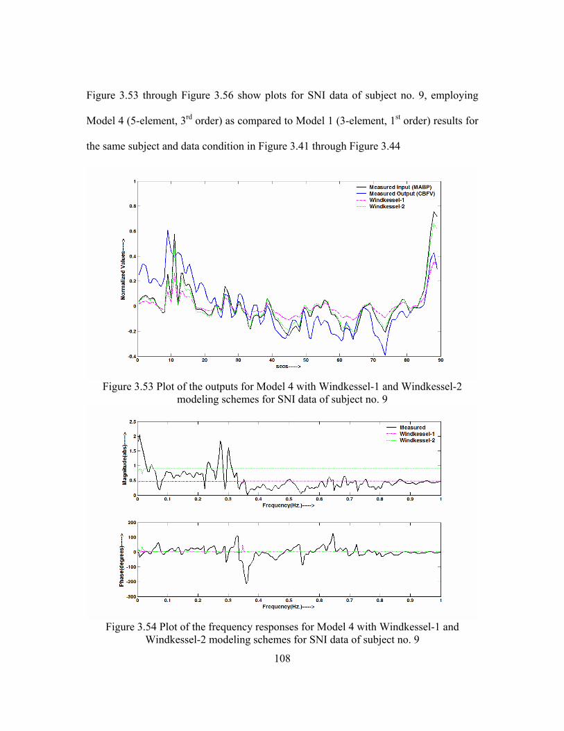
108
Figure 3.53 through Figure 3.56 show plots for SNI data of subject no. 9, employing
Model 4 (5-element, 3rd order) as compared to Model 1 (3-element, 1st order) results for
the same subject and data condition in Figure 3.41 through Figure 3.44
Figure 3.53 Plot of the outputs for Model 4 with Windkessel-1 and Windkessel-2
modeling schemes for SNI data of subject no. 9
Figure 3.54 Plot of the frequency responses for Model 4 with Windkessel-1 and
Windkessel-2 modeling schemes for SNI data of subject no. 9

109
Figure 3.55 Plot of the model outputs with ARX-1 and ARX-2 (3rd order model)
modeling schemes for SNI data of subject no. 9
Figure 3.56 Plot of the model frequency responses with ARX-1 and ARX-2
(3rd order model) modeling schemes for SNI data of subject no. 9

110
Figure 3.57 through Figure 3.60 show plots for VI data of subject no. 3, employing
Model 4 (5-element, 3rd order) as compared to Model 2 (5-element, 2nd order) results for
the same subject and data condition in Figure 3.47 through Figure 3.50
Figure 3.57 Plot of the outputs for Model 4 with Windkessel-1 and Windkessel-2
modeling schemes for VI data of subject no. 3
Figure 3.58 Plot of the frequency responses for Model 4 with Windkessel-1 and
Windkessel-2 modeling schemes for VI data of subject no. 3

111
Figure 3.59 Plot of the model outputs with ARX-1 and ARX-2 (3rd order model)
modeling schemes for VI data of subject no. 3
Figure 3.60 Plot of the model frequency responses with ARX-1 and ARX-2
(3rd order model) modeling schemes for VI data of subject no. 3

112
Figure 3.61 through Figure 3.64 show plots for VI data of subject no. 3, employing
Model 5 (4-element, 2nd order) as compared to Model 4 (5-element, 3rd order) results for
the same subject and data condition in Figure 3.57 through Figure 3.60
Figure 3.61 Plot of the outputs for Model 5 with Windkessel-1 and Windkessel-2
modeling schemes for VI data of subject no. 3
Figure 3.62 Plot of the frequency responses for Model 5 with Windkessel-1 and
Windkessel-2 modeling schemes for VI data of subject no. 3

113
Figure 3.63 Plot of the model outputs with ARX-1 and ARX-2 (2nd order model)
modeling schemes for VI data of subject no. 3
Figure 3.64 Plot of the model frequency responses with ARX-1 and ARX-2
(2nd order model) modeling schemes for VI data of subject no. 3

114
3.2.2.2 Plots for the Poor Results
Figure 3.65 Plot of the outputs for Model 1 with Windkessel-1 and Windkessel-2
modeling schemes for VI data of subject no. 2
Figure 3.66 Plot of the frequency responses for Model 1 with Windkessel-1 and
Windkessel-2 modeling schemes for VI data of subject no. 2

115
Figure 3.67 Plot of the model outputs with ARX-1 and ARX-2 (1st order model)
modeling schemes for VI data of subject no. 2
Figure 3.68 Plot of the model frequency responses with ARX-1 and ARX-2
(1st order model) modeling schemes for VI data of subject no. 2

116
Figure 3.69 Plot of the outputs for Model 2 with Windkessel-1 and Windkessel-2
modeling schemes for SNI data of subject no. 5
Figure 3.70 Plot of the frequency responses for Model 2 with Windkessel-1 and
Windkessel-2 modeling schemes for SNI data of subject no. 5
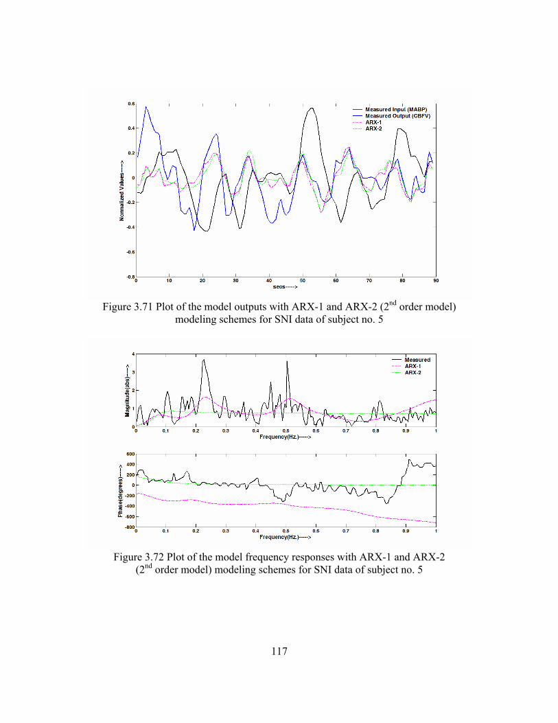
117
Figure 3.71 Plot of the model outputs with ARX-1 and ARX-2 (2nd order model)
modeling schemes for SNI data of subject no. 5
Figure 3.72 Plot of the model frequency responses with ARX-1 and ARX-2
(2nd order model) modeling schemes for SNI data of subject no. 5

118
Figure 3.73 Plot of the outputs for Model 3 with Windkessel-1 and Windkessel-2
modeling schemes for VNI data of subject no. 6
Figure 3.74 Plot of the frequency responses for Model 3 with Windkessel-1 and
Windkessel-2 modeling schemes for VNI data of subject no. 6
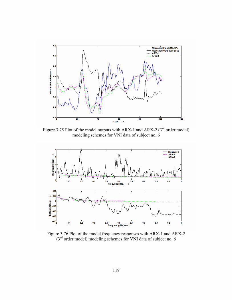
119
Figure 3.75 Plot of the model outputs with ARX-1 and ARX-2 (3rd order model)
modeling schemes for VNI data of subject no. 6
Figure 3.76 Plot of the model frequency responses with ARX-1 and ARX-2
(3rd order model) modeling schemes for VNI data of subject no. 6
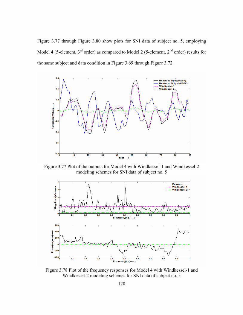
120
Figure 3.77 through Figure 3.80 show plots for SNI data of subject no. 5, employing
Model 4 (5-element, 3rd order) as compared to Model 2 (5-element, 2nd order) results for
the same subject and data condition in Figure 3.69 through Figure 3.72
Figure 3.77 Plot of the outputs for Model 4 with Windkessel-1 and Windkessel-2
modeling schemes for SNI data of subject no. 5
Figure 3.78 Plot of the frequency responses for Model 4 with Windkessel-1 and
Windkessel-2 modeling schemes for SNI data of subject no. 5

121
Figure 3.79 Plot of the model outputs with ARX-1 and ARX-2 (3rd order model)
modeling schemes for SNI data of subject no. 5
Figure 3.80 Plot of the model frequency responses with ARX-1 and ARX-2
(3rd order model) modeling schemes for SNI data of subject no. 5

122
Figure 3.81 through Figure 3.84 show plots for VI data of subject no. 2, employing
Model 4 (5-element, 3rd order) as compared to Model 1 (3-element, 1st order) results for
the same subject and data condition in Figure 3.65 through Figure 3.68
Figure 3.81 Plot of the outputs for Model 4 with Windkessel-1 and Windkessel-2
modeling schemes for VI data of subject no. 2
Figure 3.82 Plot of the frequency responses for Model 4 with Windkessel-1 and
Windkessel-2 modeling schemes for VI data of subject no. 2

123
Figure 3.83 Plot of the model outputs with ARX-1 and ARX-2 (3rd order model)
modeling schemes for VI data of subject no. 2
Figure 3.84 Plot of the model frequency responses with ARX-1 and ARX-2
(3rd order model) modeling schemes for VI data of subject no. 2
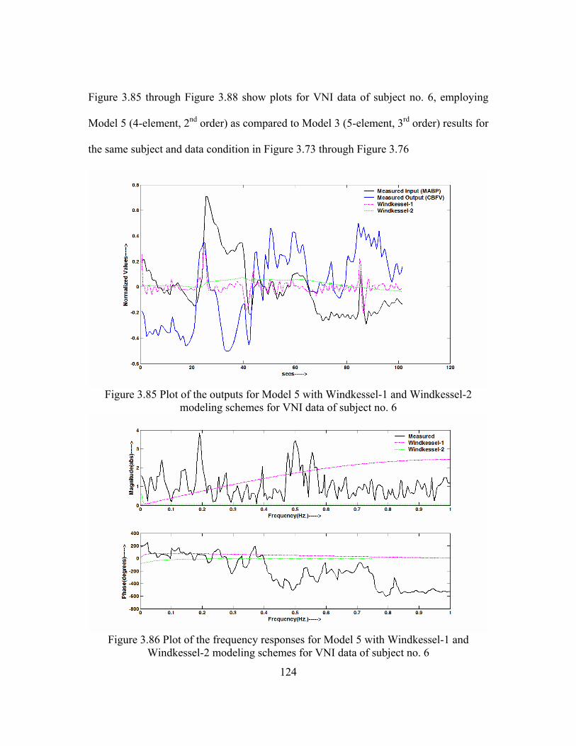
124
Figure 3.85 through Figure 3.88 show plots for VNI data of subject no. 6, employing
Model 5 (4-element, 2nd order) as compared to Model 3 (5-element, 3rd order) results for
the same subject and data condition in Figure 3.73 through Figure 3.76
Figure 3.85 Plot of the outputs for Model 5 with Windkessel-1 and Windkessel-2
modeling schemes for VNI data of subject no. 6
Figure 3.86 Plot of the frequency responses for Model 5 with Windkessel-1 and
Windkessel-2 modeling schemes for VNI data of subject no. 6
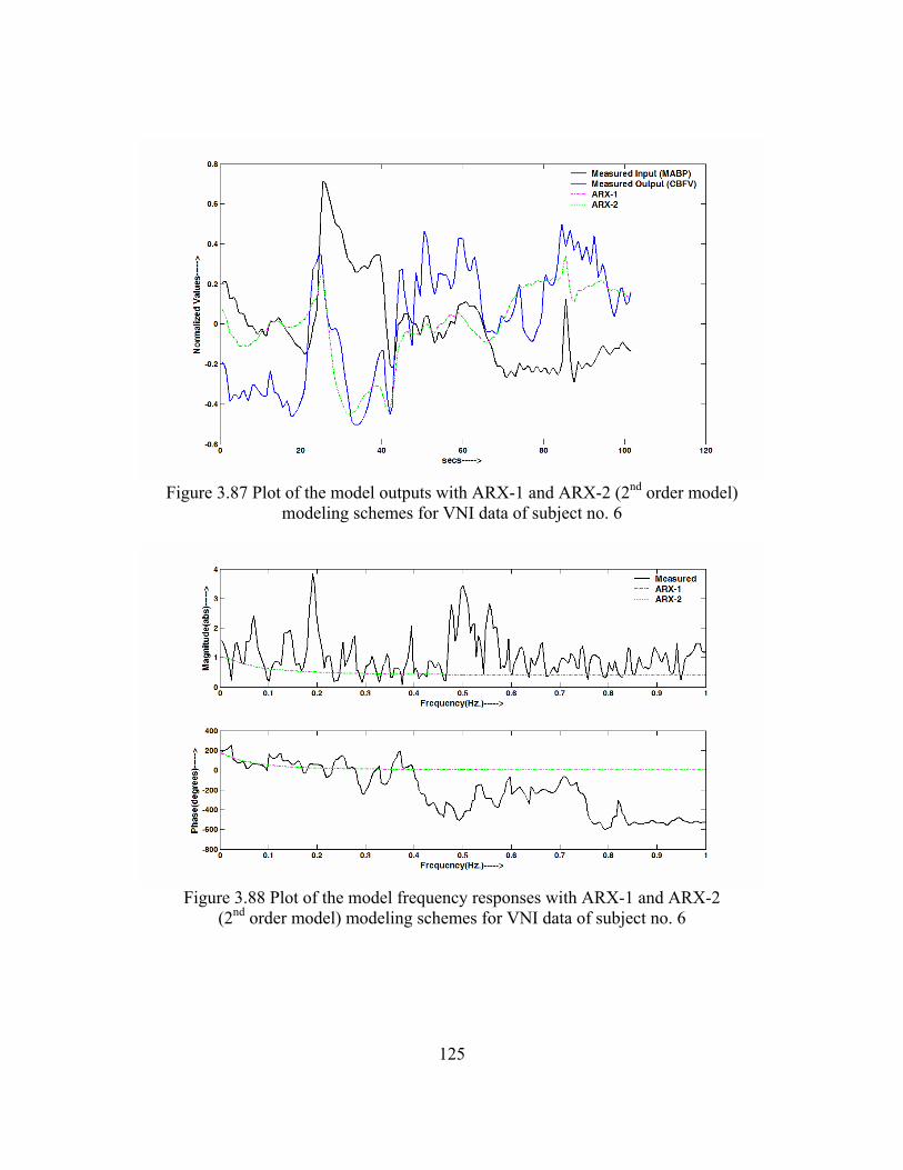
125
Figure 3.87 Plot of the model outputs with ARX-1 and ARX-2 (2nd order model)
modeling schemes for VNI data of subject no. 6
Figure 3.88 Plot of the model frequency responses with ARX-1 and ARX-2
(2nd order model) modeling schemes for VNI data of subject no. 6
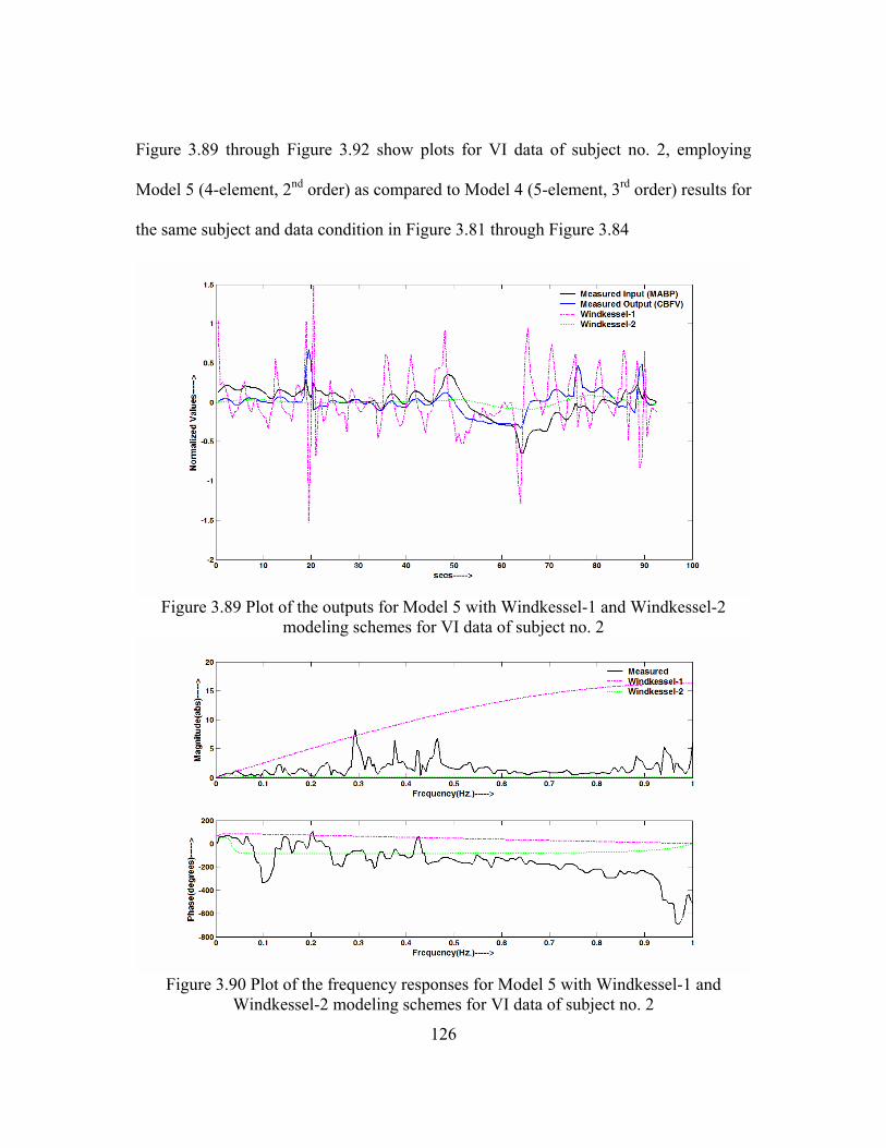
126
Figure 3.89 through Figure 3.92 show plots for VI data of subject no. 2, employing
Model 5 (4-element, 2nd order) as compared to Model 4 (5-element, 3rd order) results for
the same subject and data condition in Figure 3.81 through Figure 3.84
Figure 3.89 Plot of the outputs for Model 5 with Windkessel-1 and Windkessel-2
modeling schemes for VI data of subject no. 2
Figure 3.90 Plot of the frequency responses for Model 5 with Windkessel-1 and
Windkessel-2 modeling schemes for VI data of subject no. 2

127
Figure 3.91 Plot of the model outputs with ARX-1 and ARX-2 (2nd order model)
modeling schemes for VI data of subject no. 2
Figure 3.92 Plot of the model frequency responses with ARX-1 and ARX-2
(2nd order model) modeling schemes for VI data of subject no. 2

128
3.2.2.3 Plots for Windkessel-3 Modeling Scheme
Figure 3.93 Plot of the output for Model 1 with Windkessel-3 modeling scheme
for SNI data of subject no. 9
Figure 3.94 Plot of the frequency response for Model 1 with Windkessel-3 modeling
scheme for SNI data of subject no. 9

129
Figure 3.95 Plot of the output for Model 1 with Windkessel-3 modeling scheme
for VI data of subject no. 2
Figure 3.96 Plot of the frequency response for Model 1 with Windkessel-3 modeling
scheme for VI data of subject no. 2
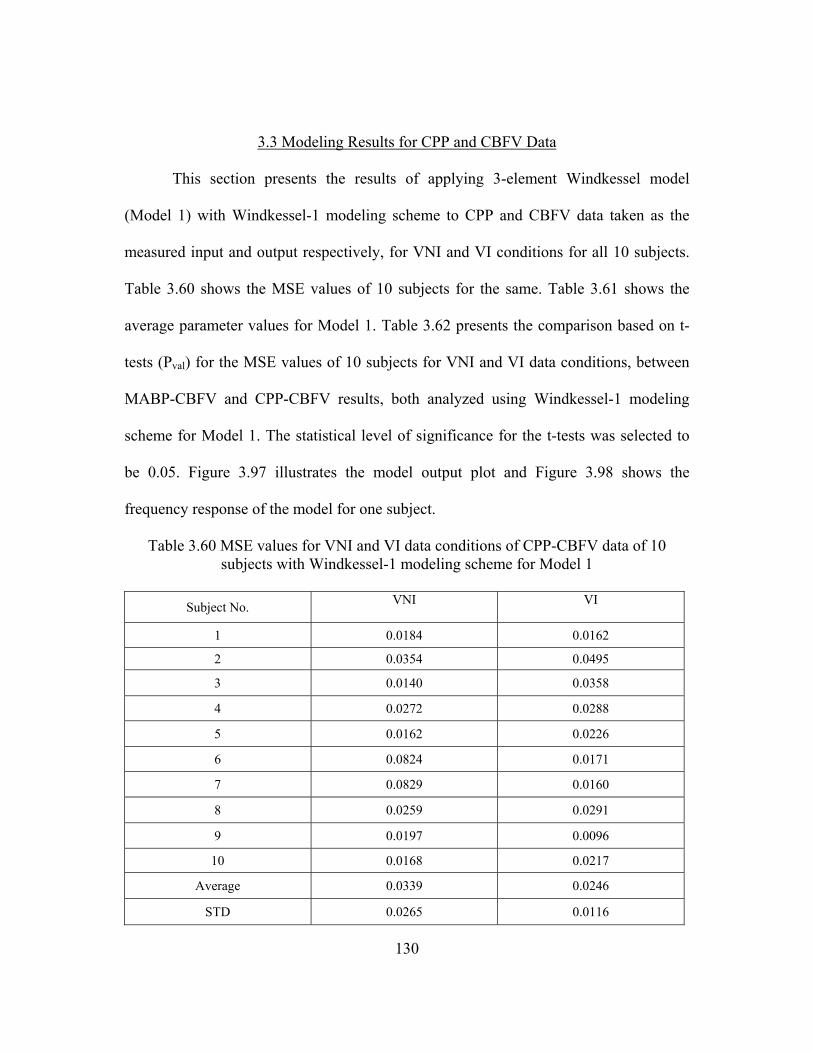
130
3.3 Modeling Results for CPP and CBFV Data
This section presents the results of applying 3-element Windkessel model
(Model 1) with Windkessel-1 modeling scheme to CPP and CBFV data taken as the
measured input and output respectively, for VNI and VI conditions for all 10 subjects.
Table 3.60 shows the MSE values of 10 subjects for the same. Table 3.61 shows the
average parameter values for Model 1. Table 3.62 presents the comparison based on t-
tests (Pval) for the MSE values of 10 subjects for VNI and VI data conditions, between
MABP-CBFV and CPP-CBFV results, both analyzed using Windkessel-1 modeling
scheme for Model 1. The statistical level of significance for the t-tests was selected to
be 0.05. Figure 3.97 illustrates the model output plot and Figure 3.98 shows the
frequency response of the model for one subject.
Table 3.60 MSE values for VNI and VI data conditions of CPP-CBFV data of 10 subjects with Windkessel-1 modeling scheme for Model 1
Subject No. VNI VI
1 0.0184 0.0162
2 0.0354 0.0495
3 0.0140 0.0358
4 0.0272 0.0288
5 0.0162 0.0226
6 0.0824 0.0171
7 0.0829 0.0160
8 0.0259 0.0291
9 0.0197 0.0096
10 0.0168 0.0217
Average 0.0339 0.0246
STD 0.0265 0.0116

131
Table 3.61 Average parameter values for VNI and VI data conditions of CPP-CBFV data of 10 subjects with Windkessel-1 modeling scheme for Model 1
R1 R2 C1
VNI Average 3.2620 10.5894 24.0239
VNI STD 5.8253 7.6332 21.8810
VI Average 2.4657 17.4151 19.9499
VI STD 2.8540 29.5489 19.8028
Table 3.62 Comparison (t-test) of MSE values of 10 subjects for VNI and VI data conditions between MABP-CBFV and CPP-CBFV using
Windkessel-1 modeling scheme for Model 1
VNI VI
Pval 0.607796 0.168638
Figure 3.97 Plot of the output for Model 1 with Windkessel-1 modeling scheme
for CPP-CBFV VI data of subject no. 2
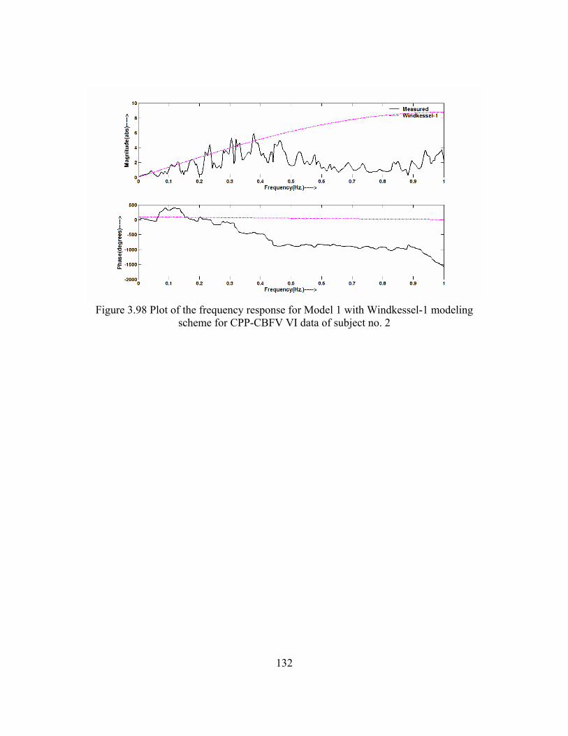
132
Figure 3.98 Plot of the frequency response for Model 1 with Windkessel-1 modeling
scheme for CPP-CBFV VI data of subject no. 2
133
CHAPTER 4
DISCUSSION AND LIMITATIONS
This section presents the important implications and discussions for the results
presented in chapter 3. Limitations to the present study have also been briefly described.
4.1 Discussion for the Results of Testing the Adequacy and Efficacy of 1.5 Minute MABP as Input Stimulus
4.1.1 ARX Models
Results from the present study show that for each of the 10 subjects, MSE
values for Ma, Me1 and Me2 models equal for the 6 minutes study. Also, for each of the
four 1.5 minute studies, the MSE values for Ma, Me1 and Me2 models were equal for a
given subject. It should be noted that the models Ma, Me1 and Me2 for each of the 10
subjects did not necessarily have identical parameters or similar orders, as is reflected in
Table 3.4. However, it is noted that the average order for models derived using MABP
and PRBS are essentially the same, regardless of what data length (i.e. 6 or 1.5 minute)
is used. It can be concluded that beat-to-beat MABP sequence is as effective as PRBS
for parametric identification of linear models. Results in Table 3.1 show that MSE
values for 1.5 minute duration studies are comparable with that of 6 minutes study. The

134
t-test results in Table 3.2 and Table 3.3 also suggest that temporal location of the four
1.5 minute sections from the 6 minutes data has no significance. This is based on the
observation that for all the cases the Pval is greater than the statistical level of
significance (0.05). Hence, it is apparent that a segment of 1.5 minute duration of
MABP is adequate for parametric system identification of cerebral autoregulation.
4.1.2 Monte-Carlo Simulation for Windkessel Models
This section discusses Windkessel-1 and Windkessel-2 modeling schemes on
the basis of Monte-Carlo simulation results (estimated-parameters and MSE values) for
the five models for both PRBS and MABP input. Comparing the two modeling
techniques, the performance of Windkessel-2 scheme was apparently better than
Windkessel-1 scheme, based on the average MSE values and comparison of true-
parameters (Ma) and estimated-parameters (Me). However, results from both schemes
point that MABP sequence is as effective and efficient as PRBS for parametric
identification of linear models, and also that 1.5 minute duration is adequate for the
same.
4.1.2.1 Windkessel-1 Modeling Scheme
Results from the present study show that for Model 1, Model 2 and Model 4, the
estimated parameters (Me) were reasonably close to the parameters obtained for model
Ma, using PRBS or MABP as input. This is also reflected in the histograms of true-
parameter values and estimated parameter values for the resistance parameter R1 for
each of these three models. For both PRBS and MABP input, the resistance parameter
R1 of Model 3 and Model 5 were poorly estimated, which is reflected in their

135
corresponding true-parameter value and estimated-parameter value histograms. For the
same reason the average MSE values for models 3 and 5 were poor and not comparable
to the average MSE values of the other three models, as is shown in Table 3.10 and
Table 3.16. However, this being the case for both MABP and PRBS input, the average
MSE values for respective models in both cases (Table 3.10 and Table 3.16) are similar
and comparable. Noting that both the PRBS and MABP were 1.5 minute duration
sequences, it can be concluded that MABP sequence is as good as PRBS for parametric
identification of linear models, and also that a duration of 1.5 minute is adequate for the
same.
The poor estimates of the true-parameter value of R1 in case of Model 3 and
Model 5 for both PRBS and MABP can be explained from limitation of the Windkessel-
1 modeling scheme. The basis of this scheme is the evaluating R1 from the model
transfer function, as explained in section 2.2.3.2. This type of approach of extracting R1
by applying the limit of frequency ω tending to infinity to the modulus of the transfer
function is an approximation, because the actual signal (MABP, CBFV) is the case of
this study is sampled at 2 Hz (section 2.1.4). Hence the highest frequency point of the
measured impedance curve, Zm, is at only 1 Hz and not infinity, which may result in
poor estimation of resistance parameter R1, by extracting its value from that point
(Equations 2.11, 2.12, and 2.13). This in turn is reflected by higher MSE values for the
cases where R1 is poorly estimated. Furthermore, this approximation technique is
affected by presence of noise in the Zm.

136
4.1.2.2 Windkessel-2 Modeling Scheme
Results from the present study show that for all the five models, the estimated
parameters (Me) were reasonably close to the true-parameters (Ma), for the PRBS as
well as MABP input. This is also reflected in the histograms of true-parameter value
and estimated parameter value for the resistance parameter R1 for each of these three
models. For both PRBS and MABP input, the Ma and Ma were exactly the same (up to
the fourth place of the decimal) for Model 5, as is reflected in Table 3.21 and Table 3.27
and Figure 3.29, Figure 3.30, Figure 3.39, and Figure 3.40. Also, the average MSE
values for the five models for both PRBS and MABP input (Table 3.22 and Table 3.28)
are fairly close. Noting that both the PRBS and MABP were 1.5 minute duration
sequences, it can be concluded that MABP sequence is as good as PRBS for parametric
identification of linear models, and also that a duration of 1.5 minute is adequate for the
same.
Apart from establishing the effectiveness and adequacy of 1.5 minute MABP
sequence, the Monte-Carlo simulation results play an important role in establishing the
effectiveness and accuracy of Windkessel models and modeling schemes. The
simulation serves as an exhaustive test for the Windkessel estimation algorithms, testing
the estimation techniques on a large number of randomly simulated parameters, with
other factors, like the initial estimates for optimization routines, also being random.

137
4.2 Discussion of the Modeling Results for MABP and CBFV Data
This section discusses and compares the ARX-1, ARX-2, Windkessel-1,
Windkessel-2, and Windkessel-3 modeling schemes on the basis of MSE values of 10
subjects for the four data conditions (i.e. SNI, SI, VNI, VI), and plots illustrated in
section 3.2.2.
4.2.1 ARX Models
The ARX-1 modeling scheme results in average model orders of 8.5, 6.6, 5.9,
and 4.2 for respectively the SNI, SI, VNI, and VI data sets (Table 3.30). It is important
to note that for ARX-1 scheme and for 1st, 2nd, and 3rd order models of ARX-2 scheme,
for subject no. 9, VI data (1.5 minute) the models produced unstable model outputs, as
is reflected by the corresponding MSE values in Table 3.29, Table 3.31, Table 3.33, and
Table 3.35. In the same context, the MSE value was lowest for the 1st order model and
highest for the 3rd order model. This is also shown in Table 3.30 for ARX-1 scheme,
where for subject no. 9, VI case, the best model among 1st to 10th order models turned
out to be a 1st order model.
Even though the average MSE values for ARX-1 scheme are lower than 1st, 2nd,
and 3rd order models of ARX-2 scheme, the MSE values for ARX-1 scheme (Table
3.29) are close to the MSE values produced by the 1st order model of ARX-2 modeling
scheme (Table 3.31), and if the MSE value of the model for subject no. 9, VI case, is
ignored for both ARX-1 and ARX-2 scheme, the MSE values are relatively close for
ARX-1 scheme and all the three models of ARX-2 scheme. This, combined with the
fact that in Table 3.30 one can find a number of models with orders 4 or less, implies

138
that for ARX estimation, the increase of the model order doesn’t improve the MSE
value substantially. Moreover, an increase in order and may deteriorate the MSE value,
as in VI case of subject no. 9 for the present study.
4.2.2 Windkessel Models
From the results in Appendix B, it is clear that there is no significant difference
between the MSE values produced by Windkessel-1, Windkessel-2 and Windkessel-3
modeling schemes for the four data conditions of 10 subjects, for each of the five
models. This is based on the t-test comparisons of the three modeling schemes with
each other for a given model, which resulted in Pval is greater than the statistical level of
significance (0.05). However, in terms of the average MSE values of the five models for
Windkessel-1 and Windkessel-2 modeling schemes and of Model 1 for Windkessel-3
modeling scheme (section 3.2.1.2), for a given model, Widkessel-2 scheme produced
lower average MSE values than Windkessel-1 and Windkessel-3 schemes. It is
important to note that within the five models for the four data conditions, the average
MSE values were relatively close for all the five models, this being true for both
Windkessel-1 and Windkessel-2 scheme. It is also relevant to mention that the average
values of the weights Wt and Wf for the four data conditions (Table 3.59),
corresponding to Windkessel-3 modeling scheme for Model 1, show that for achieving
a lower MSE value in time domain, the algorithm tried to improve frequency domain
response of the model to fit it better to the measured one. This inference is based on the
result that the average value of weighing-parameter for frequency domain MSE (Wf)
139
was higher, and almost double the average value of weighing-parameter for the time
domain MSE (Wt), for all the four data conditions.
Comparing MSE values for ARX-2 with Windkessel-1 and Windkessel-2
schemes for models with similar order, the results in Appendix B demonstrated
significant difference in SNI data condition for Windkessel Model 2, Model 3, Model 4
and Model 5. This is based on the t-test results where Pval is smaller than the statistical
level of significance (0.05). This is also reflected by the average MSE values for SNI
data condition with Windkessel-1 and Windkessel-2 schemes for all the five models,
which were higher than the ARX-2 scheme models of similar order for SNI data set.
For rest of the ARX-2 scheme comparisons with the three Windkessel schemes, no
significant level of difference was observed. Comparing the ARX-1 methodology with
the Windkessel schemes, the average MSE values for SNI, SI and VNI data conditions
for ARX-1 modeling technique were lower than the corresponding average MSE values
of the three Windkessel modeling schemes for all the five models.
4.2.3 Graphical Validation
Section 3.2.2 presented samples of the time-domain output and frequency
response plots as good and poor results based on MSE value of the Windkessel-1
methodology in each model and type of data condition. Visually observing the plots for
good results in section 3.2.2.1, Figure 3.41 shows that Model 1 for both Windkessel-1
and Windkessel-2 scheme followed the measured output of SNI data for subject no. 9
pretty well. In terms of frequency response, Windkessel-1 scheme matched the
measured magnitude response better than Windkessel-2 scheme, and as is expected,

140
Windkessel-1 scheme magnitude almost meets the measured magnitude response curve
at the highest frequency point of 1 Hz. For the same subject and data condition, ARX-1
and ARX-2 plots in Figure 3.43 were also quite comparable to each other, as well as to
both of the Windkessel plots in Figure 3.41. But ARX-1 scheme produces a better
frequency response comparable to measured one (Figure 3.44), which may be due to
higher order models associated with ARX-1 scheme. In Figure 3.45, for VI data of
subject no. 3, Model 2 for both the Windkessel schemes produces a good fit of the
measured output. For the same subject and data condition, the two ARX schemes in
Figure 3.47 did not follow the measured output as well as the Windkessel schemes. It is
important to note here that Windkessel schemes had a magnitude response which
matched the measured response better at the low frequencies (0.0 – 0.2 Hz), as seen in
Figure 3.46, and ARX schemes produced a magnitude response which matched the
measured one better at the high frequencies (0.6 – 1.0 Hz), as seen in Figure 3.48.
Figure 3.49 shows how the Model 3 for the two Windkessel schemes followed the
measured output for VNI data of subject no. 1. For the same subject and data condition,
the two ARX schemes in Figure 3.51 followed the low-frequency changes better,
including the high peaks and the low dips of the measured output. This is somewhat
evident from the comparison of the magnitude responses of Windkessel schemes in
Figure 3.50 and ARX schemes in Figure 3.52. Figure 3.53 and Figure 3.55 illustrate the
model outputs of Model 4 for Windkessel schemes and of 3rd order model for ARX-2
scheme respectively, for SNI data of subject no. 9. It is worthwhile to note that the
responses in both these figures are comparable to the responses of Figure 3.41 and

141
Figure 3.43, for the same subject and data condition; however the model in the latter
case is lower in order and number of elements than the model in the former case, for the
ARX-2 and both of the Windkessel schemes. Also, the frequency responses of the two
cases are quite similar. A similar observation can be made while comparing the Figure
3.45 with Figure 3.57, and Figure 3.47 with Figure 3.59, for VI data of subject no. 3.
Model 5 in Figure 3.61 for VI data of subject no. 3 followed the measured output better
in case of Windkessel-1 scheme. The difference in the magnitude response at low
frequencies (0.0 – 0.1 Hz) of the two Windkessel schemes in Figure 3.62 is prominent.
The two ARX schemes in Figure 3.63 could not perform as good as the Windkessel
schemes.
Visually observing the plots for poor results in section 3.2.2.2, Model 1 for both
Windkessel schemes in Figure 3.65 failed to follow the measured output for VI data of
subject no. 2. Also, the model frequency responses for same in Figure 3.66 did not
match the measured response. For the same subject and data condition, ARX-1
modeling scheme in Figure 3.67 produced a better result, which also is evident from the
frequency response of ARX-1 model in Figure 3.68. Figure 3.69 shows that Model 2 for
Windkessel-1 scheme had a comparatively better result than Windkessel-2 scheme, for
SNI data of subject no. 5; this can also be seen in the magnitude response of
Windkessel-1 scheme in Figure 3.70. For the same subject and data condition, both
ARX-1 and ARX-2 modeling scheme in Figure 3.71 produced a superior result than
Windkessel schemes. A similar observation can be made for the Windkessel results for
Model 3 in Figure 3.73 and ARX results in Figure 3.75, for VNI data of subject no. 6.

142
Figure 3.77 and Figure 3.79 for SNI data of subject no. 5 shows that going to a higher
order and higher element model did not produce any improvements in the model fit to
the measured data, as compared to Figure 3.69 and Figure 3.71 respectively for the
same subject and data condition. Likewise, a similar observation can be made while
comparing the Windkessel results for Model 4 for VI data of subject no. 2 in Figure
3.81 and for Model 1 in Figure 3.65, for the same subject and data condition. Figure
3.85 shows that Model 5 for Windkessel-1 scheme had a comparatively better result
than Windkessel-2 scheme, for VNI data of subject no. 6. For the same subject and data
condition, both ARX-1 and ARX-2 modeling scheme in Figure 3.87 produced a
superior result than Windkessel schemes. Figure 3.89 for VI data of subject no. 2 shows
no improvements for Model 5 with Windkessel schemes, as compared to Figure 3.65
and Figure 3.81. Again, both ARX schemes in Figure 3.91 produced better results for
the same subject and data condition. Plot for Model 1 with Windkessel-3 modeling
scheme in Figure 3.93 has no significant difference as compared to Windkessel-1 and
Windkessel-2 schemes in Figure 3.41 and Figure 3.53. However, Model 1 with
Windkessel-3 scheme in Figure 3.95 for VI data of subject no. 2 shows significant
improvement when compared to Figure 3.65, Figure 3.81 and Figure 3.89.
From the MSE value comparisons and discussion of the plots, it is clear that in
Windkessel schemes, Windkessel-1 modeling scheme is superior to Windkeseel-2
modeling scheme. The apparent reason for which is the magnitude response in case on
Windkessel-1 scheme which is forced to the match the measured magnitude response
curve, Zm, by extracting the resistance parameter R1 form Zm and fixing its value by not

143
optimizing it. For results with Model 1, Windkessel-3 scheme seems promising in terms
of graphical validation results, but the average MSE values for the four data conditions
in this scheme is larger than Windkessel-1 and Windkessel-2 schemes for Model 1.
Comparing the five Windkessel models, there was no significant difference in the MSE
values for both Windkessel-1 and Windkessel-2 schemes (Appendix B). In the plots for
good results where the model response followed the measured output closely, for the
same subject and data condition higher element models produced no significant
improvement. This was also the case when the model output did not follow the
measured output well. The two ARX schemes are comparable to each other in terms of
average MSE values and the proximity of the model output to the measured output, but
are better than the Windkessel schemes in both the MSE results and the proximity of the
model output to the measured output, ignoring the case for VI data of subject no. 9,
where both the ARX schemes produced unstable models.
Comparing MSE values and parameter values of the data conditions with and
without infusion (i.e. SNI vs. SI, VNI vs. VI) for the five Windkessel models with
Windkessel-1 modeling scheme (Appendix B), it can be seen that there was no
significant difference observed. Also, the comparison results of MSE values and
parameter values of the data conditions with and without infusion for 1st order model
with ARX-1 modeling scheme showed a lack of significance for most of the p values
(Appendix B). The statistical level of significance for all of these results was taken as
0.05. These outcomes show that the blockade of autonomic neural activity by drug
infusion in the measured data could not be reproduced by the models in their MSE and

144
parameter values of the models, even though the effect of blockade can be observed in
the spontaneous (SNI, SI) as well as Valsalva maneuver (VNI, VI) conditions of the
measured data (Figures 2.1 through 2.4) in terms of MABP and CBFV values and the
four recognized Valsalva maneuver phases (section 2.1.3). This indicates that ganglion
blockade did not have a noteworthy effect on the MSE and parameter values of the
ARX and Windkessel models.
4.3 Discussion of the Modeling Results for CPP and CBFV Data
Table 3.60 presents the MSE values associated with Windlkessel-1 scheme of
Model 1 for CPP-CBFV VNI and VI data of 10 subjects. Comparing the average MSE
values with the corresponding average MSE values for MABP-CBFV data in Table
3.37, there was a slight deterioration in the average MSE value for VNI case of CPP-
CBFV data, but the VI case showed improvement. However, results for the comparison
(t-test) of CPP-CBFV and MABP-CBFV in Table 3.62 show a Pval greater than 0.05 for
VNI and VI, indicating no significant level of difference for the two cases. Plot in
Figure 3.97 for VI data of subject no. 2 shows no significant improvement when
compared to Figure 3.65, Figure 3.81 and Figure 3.89. These results weaken the
conjecture of using CPP-CBFV data for linear modeling of cerebral autoregulation to
yield better results as compared to using MABP-CBFV data.

145
4.4 Limitations
All of the modeling methods discussed in the present study rely on the
assumption that the dynamic autoregulatory mechanism can be approximated by a
linear system, ignoring several nonlinearities, like those related to fluid flow. It has been
assumed that the MABP and CBFV are correlated without taking into account any
phase lag or feedback action between them. Another presumption is that the middle
cerebral artery (MCA), where CBFV is measured, does not change its diameter. This
presumption was important to this study as the TCD technique used measures velocity
of blood flow in the MCA, rather than the volumetric or mass flow rate of blood in
MCA. Also, regarding the measurement of MABP in finger using
photoplethysmography technique, the arterial pressure waveforms in the finger may be
different from that in the MCA due to pressure wave reflection and amplification in the
peripheral vascular bed. With respect to the CPP-CBFV data, the estimation of CPP was
done from the MABP data, whereas, to assess changes in CPP, MABP should be
measured simultaneously with ICP and/or CVP. With respect to results from the present
study, an important limitation is that for Windkessel models, different parameter values
associated with the resistive (R), capacitive (C) and inductive (L) elements could result
into similar and comparable MSE values. This indicates that these model parameters are
not distinctive and unique.

146
CHAPTER 5
CONCLUSION AND DIRECTIONS FOR FUTURE WORK
5.1 Conclusions
The present study is focused on employing single input single output linear
lumped parametric models (ARX and Windkessel) to beat-to-beat mean arterial blood
pressure (MABP) considered as input to the model, and cerebral blood flow velocity
(CBFV) considered as output of the model. For some models and modeling
methodologies, the data consisted of cerebral perfusion pressure (CPP, estimated from
MABP) and CBFV. The measurement of the data from the subjects was done while the
subjects were performing Valsalva maneuver with and without the use of trimethaphan
for ganglion blockade, the infusion of which essentially removes the autonomic neural
activity. The main objective of this study was to examine the relative performance and
limitations of the above mentioned linear modeling options and to demonstrate newer
modeling methodologies for them. Another purpose of this study was to examine and
establish the efficacy of beat-to-beat blood pressure time sequence in serving as an
input stimulus, and to investigate the use of a short data segment of 1.5 minute changes
in MABP for obtaining linear model estimation of cerebral autoregulation.

147
Results from chapter 3 and their discussion in chapter 4 suggest that linear
system method for parametric identification of pressure-flow relationship of cerebral
circulation is feasible. The models used for the present study had very simple and basic
mechanisms and structures, but were still able to reproduce the measured data. Even
though the modeling methodologies for the study were not restricted to lower order
systems, and examined even 10th ordered systems in case of ARX models and higher
element models in case of Windkessel models, results indicate that lower order ARX
models (1st, 2nd, and 3rd order models for ARX-2 scheme) and 3-element Windkessel
model (Model 1) may be adequate. Among the ARX and Windkessel methodologies,
ARX modeling schemes produced superior results. Windkessel-1 modeling scheme
turns out to be better than Windkeseel-2 modeling scheme. Also, for results with Model
1, Windkessel-3 scheme seems promising in terms of graphical validation results. The
results of using CPP-CBFV data did not prove to be better than MABP-CBFV data
results, for Model 1 with Windkessel-1 scheme. Comparing MSE values and parameter
values of the data conditions with and without infusion (i.e. SNI vs. SI, VNI vs. VI) for
the five Windkessel models with Windkessel-1 modeling scheme and for 1st order
model with ARX-1 modeling scheme, it can be seen that the ganglion blockade did not
have a significant effect on the MSE and parameter values of the ARX and Windkessel
models.
From the results of testing the adequacy and efficacy of 1.5 minute MABP as
input stimulus by ARX models, it can be concluded that a data segment of 1.5 minute
duration of changes in MABP is adequate for parametric system identification of

148
cerebral circulation. This conclusion is strengthened by the results for Monte-Carlo
simulations of Windkessel models using Windkessel-1 and Windkessel-2 schemes with
MABP and PRBS as inputs. Hence it is clear that a segment of 1.5 minute duration of
MABP is effective and adequate for estimating linear models of cerebral autoregulation.
5.2 Directions for Future Work
Even though the various modeling methodologies employed in the present study
were able to model the cerebral circulation data in conjunction with Valsalva maneuver
for ganglion blockade, all of them were linear parametric modeling techniques. Hence it
would be of interest for future investigation to determine if other modeling techniques
involving non-parametric techniques, non-linear analysis or neural network modeling
can improve the time-domain and frequency-domain response of the models. Also, the
present study was limited to applying Windkessel-3 modeling scheme to Model 1 using
CPP-CBFV data. Future work can involve applying this scheme to other models as
well. Some other important points to be considered for future investigation of the
MABP-CBFV data include analyzing the coherence levels of input and output, and
residual analysis of the data and model to examine a feedback relationship between
MABP and CBFV. Also, it would be of immense interest to quantitatively analyze the
results for the parameters of various models in the present study to extract clinical
findings and implications from them. This may be useful for identifying patients at risk
for cerebrovascular events. Clearly, more number of subjects will be required for this
type of study.

149
APPENDIX A
DATA ANALYSIS ALGORITHMS AND PROGRAMS

150
A1 Program Used for ARX-1 Modeling Scheme described in Section 2.2.1.1
% estimation of model for system order from 1 to 10, and then selection of % best model on the basis of MSE subname = {'Brian','Dak','Danial','Danny','Fennig','Janet','Ronnie','Sandra','Steve','Vineet'}; % subject files addfix={'abpcbfv_sni','abpcbfv_si','abpcbfv_vni','abpcbfv_vi'}; % data condition subcase_vni=[1,1,1,2,1,2,2,2,2,3]; subcase_vi= [3,3,1,4,4,1,2,4,3,3]; h=waitbar(0,'Please wait..........') for ct=1:4 for vr1 = 1:10 waitbar(((10*(ct-1))+vr1)/40,h); vr2=char(strcat(subname(vr1),addfix(ct))); if (ct==3) vr2=strcat(vr2,num2str(subcase_vni(vr1))); end if (ct==4) vr2=strcat(vr2,num2str(subcase_vi(vr1))); end a1=load (strcat(vr2,'rsmp.m'),'-ascii'); u1=dtrend(a1(:,2)); u1_=u1./(max(u1)-min(u1)); % MABP v2=0; for var1=1:length(a1(:,1)) v2(var1,1)=0.1257*a1(var1,1); end v1=dtrend(v2); v2_=v1./(max(v1)-min(v1)); % CBFV z1 = [v2_ u1_]; par=0; ctr=0; for no = 2:11 % numerator order for do = 1:10 % denominator order if (no-1) <= do ctr=ctr+1; th2=arx(z1,[do,no,0]); % ARX identification th1=sett(th2,0.5); [NUM,DEN] = TH2TF(th1,1); tmp3=zeros(1,22);

151
A1 Continued.
for tmp4=1:length(NUM) tmp3(1,tmp4+(11-length(NUM)))=NUM(1,tmp4); end for tmp4=1:length(DEN) tmp3(1,tmp4+(22-length(DEN)))=DEN(1,tmp4); end par(ctr,1:22)=tmp3; end end end
% calculation of MSE values for model for system order from 1 to 10 for the subject for selection of best model
ctr=0; mse=0; tmp5=par; for no = 2:11 for do = 1:10 if (no-1) <= do ctr=ctr+1; n(1,1:11)=tmp5(ctr,1:11); d(1,1:11)=tmp5(ctr,12:22); tmp1=0; for tmp2=1:length(u1_) tmp1(tmp2,1)=tmp2*0.5; end P1=[tmp1 u1_]; % input to the simulink model Timespan=[0.5 length(u1_)/2]; sim('ARX_analysis',Timespan);
msetime=(sum((v2_(1:length(v2_),1)- v1_(1:length(v1_),1)).^2))/length(v1_);
mse(ctr,1)=msetime; end end end mse1=min(mse); par1=tmp5(find(mse==mse1),:); save(strcat(vr2,'_ARX.m'),'par1','-ascii'); end end close(h);

152
A2 Program Used for Monte-Carlo Simulation of Model 1 for Windkessel-1 Modeling Scheme with MABP (SNI) as Input described in Section 2.2.3.2 and Section 2.3.2
% Monte Carlo Simulation subname = {'Brian','Dak','Danial','Danny','Fennig','Janet','Ronnie','Sandra','Steve','Vineet'}; % subject files rand('state',0); h=waitbar(0,'Simulation in progress..........') for itr=1:1:1000 % 1000 trial simulation waitbar(itr/1000) randm3=rand(1,1);
vr1=round((randm3*9)+1); % random selection of subject SNI data between subjects 1-10
vr2=char(strcat(subname(vr1),'abpcbfv_sni')); a1=load (strcat(vr2,'rsmp.m'),'-ascii'); u1=dtrend(a1(:,2)); u1_=u1./(max(u1)-min(u1)); % MABP tmp1=0; for tmp2=1:length(u1_) tmp1(tmp2,1)=tmp2*0.5; end P1=[tmp1 u1_]; % input to the simulink model Timespan=[0.5 length(u1_)/2]; randm1=rand(3,1); Rs=(randm1(1,1)*7)+7; % parameter R1 Rp=(randm1(2,1)*5)+3; % parameter R2 Cap=(randm1(3,1)*4)+1; % parameter C1 a=(Cap*Rs*Rp); b=(Rs+Rp); c=(Cap*Rp); sim('mcarlo_sim',Timespan); w=hanning(512); Syx=xcorr(v1_,u1_); Sxx=xcorr(u1_); Pmu1 = psd(Sxx,512,2,w,256); Pmv1 = psd(Syx,512,2,w,256); Suf=0; Svf=0;

153
A2 Continued.
for k=1:length(Pmu1) Suf(k,1)=(Pmu1(k,1))^0.5; Svf(k,1)=(Pmv1(k,1))^0.5; end Z1m1 = Svf./Suf; for var1=1:256 fr(var1,1)=2*(var1/512); % Fs = 2 Hz end Z1m=Z1m1(1:256,1); % measured impedance randm2=rand(2,1); % frequency-domain optimization Rs1a = 1/Z1m(256,1); % extraction of R1 from Z1m
options=optimset('MaxFunEvals',1000000,'MaxIter',1000000,'TolFun',1.e-10,'TolCon',1.e-1,'TolX',1.e-10);
x1=0; x1=fminimax(@optfun_olufsen3,[(randm2(1,1)*5)+3,(randm2(2,1)*4)+1],[],[],[],[],[3,1],[8,5],[],options,Z1m,Rs1a);
x1(1,3)=x1(1,2); x1(1,2)=x1(1,1); x1(1,1)=Rs1a; % time-domain optimization
options=optimset('MaxFunEvals',1000000,'MaxIter',1000000,'TolFun',1.e-10,'TolCon',1.e-1,'TolX',1.e-10);
x=0; x=fminimax(@optfun_subjects4,[x1(1,2),x1(1,3)],[],[],[],[],[3,1],[8,5],[], options,u1_,v1_,Rs1a);
y2=idsim(u1_,thc2thd(poly2th(1,[1/Rs1a 1/(x(1,2)*x(1,1)*Rs1a)],1,1,[1 (x(1,1)+Rs1a)/(x(1,2)*x(1,1)*Rs1a)],1,0),0.5)); mse1(itr,1)= (sum((y2(1:length(y2),1)- v1_(1:length(v1_),1)).^2))/length(v1_); % storing the MSE value for time domain
param1(itr,1)= Rs; % storing the true parameters for respective run param1(itr,2)= Rp; param1(itr,3)= Cap;
param2(itr,1)= Rs1a; % storing the estimated parameters for respective run
param2(itr,2)= x(1,1); param2(itr,3)= x(1,2); end close(h)

154
A2 Continued.
A3 Program Used for Monte-Carlo Simulation of Model 1 for Windkessel-2 Modeling Scheme with MABP (SNI) as Input described in Section 2.2.3.3 and Section 2.3.2
save true_parameters.m param1 -ascii save estimated_parameters.m param2 -ascii save mse_timedomain.m mse1 -ascii save mse_freqdomain.m mse2 -ascii % function used for frequency-domain optimization %x1(1)=R2 %x1(2)=C1 function f = optfun_olufsen3(x1,Z1m,Rs1a) for k=1:256 w(k,1)=2*(k/512); Zw(k,1)=abs((1+i*(w(k,1)*x1(2)*x1(1)))/(x1(1)+Rs1a+i*(w(k,1)*x1(2)* Rs1a*x1(1)))); end f = sum((Zw(1:256,1)-Z1m(1:256,1)).^2); % function used for time-domain optimization %x(1)=R2 %x(2)=C1 function f = optfun_subjects4(x,u1_,v1_,Rs1a) y1=idsim(u1_,c2d(poly2th(1,[1/Rs1a 1/(x(2)*x(1)*Rs1a)],1,1, [1 (x(1)+Rs1a)/(x(2)*x(1)*Rs1a)],1,0),0.5)); f = sum(((y1(1:length(y1),1)-v1_(1:length(v1_),1)).^2));
%Monte Carlo Simulation subname = {'Brian','Dak','Danial','Danny','Fennig','Janet','Ronnie','Sandra','Steve','Vineet'}; % subject files rand('state',0); h=waitbar(0,'Simulation in progress..........') for itr=1:1:1000 % 1000 trial simulation waitbar(itr/1000) randm3=rand(1,1); vr1=round((randm3*9)+1); % random selection of subject SNI data vr2=char(strcat(subname(vr1),'abpcbfv_sni')); a1=load (strcat(vr2,'rsmp.m'),'-ascii');

155
A3 Continued.
u1=dtrend(a1(:,2)); u1_=u1./(max(u1)-min(u1)); % MABP tmp1=0; for tmp2=1:length(u1_) tmp1(tmp2,1)=tmp2*0.5; end P1=[tmp1 u1_]; % input to the simulink model Timespan=[0.5 length(u1_)/2]; randm1=rand(3,1); Rs=(randm1(1,1)*7)+7; % parameter R1 Rp=(randm1(2,1)*5)+3; % parameter R2 Cap=(randm1(3,1)*4)+1; % parameter C1 a=(Cap*Rs*Rp); b=(Rs+Rp); c=(Cap*Rp); sim('mcarlo_sim',Timespan); w=hanning(512); Syx=xcorr(v1_,u1_); Sxx=xcorr(u1_); Pmu1 = psd(Sxx,512,2,w,256); Pmv1 = psd(Syx,512,2,w,256); Suf=0; Svf=0; for k=1:length(Pmu1) Suf(k,1)=(Pmu1(k,1))^0.5; Svf(k,1)=(Pmv1(k,1))^0.5; end Z1m1 = Svf./Suf; for var1=1:256 fr(var1,1)=2*(var1/512); % Fs = 2 Hz end Z1m=Z1m1(1:256,1); % measured impedance randm2=rand(2,1); % frequency-domain optimization Rs1a = 1/Z1m(256,1); % extraction of R1 from Z1m
options=optimset('MaxFunEvals',1000000,'MaxIter',1000000,'TolFun', 1.e-10,'TolCon',1.e-1,'TolX',1.e-10); x1=0;

156
A3 Continued.
x1=fminimax(@optfun_olufsen3_2,[(randm2(1,1)*5)+3,(randm2(2,1)*4)+1] ,[],[],[],[],[3,1],[8,5],[],options,Z1m,Rs1a); x1(1,3)=x1(1,2); x1(1,2)=x1(1,1); x1(1,1)=Rs1a; % time-domain optimization
options=optimset('MaxFunEvals',1000000,'MaxIter',1000000,'TolFun', 1.e- 10,'TolCon',1.e-1,'TolX',1.e-10);
x=0; x=fminimax(@optfun_subjects4_2,[x1(1,1),x1(1,2),x1(1,3)],[],[],[],[], [7,3,1],[14,8,5],[],options,u1_,v1_);
y2=idsim(u1_,thc2thd(poly2th(1,[1/x(1,1) 1/(x(1,3)*x(1,2)*x(1,1))],1,1,[1 (x(1,2)+x(1,1))/(x(1,3)*x(1,2)*x(1,1))],1,0),0.5)); mse1(itr,1)= (sum((y2(1:length(y2),1)- v1_(1:length(v1_),1)).^2))/length(v1_); % storing the MSE value for time domain
param1(itr,1)= Rs; % storing the true parameters for respective run param1(itr,2)= Rp; param1(itr,3)= Cap; param2(itr,1)= x(1,1); % storing the estimated parameters for respective run param2(itr,2)= x(1,2); param2(itr,3)= x(1,3); end close(h) save true_parameters.m param1 -ascii save estimated_parameters.m param2 -ascii save mse_timedomain.m mse1 -ascii save mse_freqdomain.m mse2 –ascii % function used for frequency-domainoptimization %x1(1)=R2 %x1(2)=C1 function f = optfun_olufsen3_2(x1,Z1m,Rs1a) for k=1:256 w(k,1)=2*(k/512); Zw(k,1)=abs((1+i*(w(k,1)*x1(2)*x1(1)))/(x1(1)+Rs1a+i*(w(k,1)*x1(2)* Rs1a*x1(1)))); end f = sum((Zw(1:256,1)-Z1m(1:256,1)).^2);
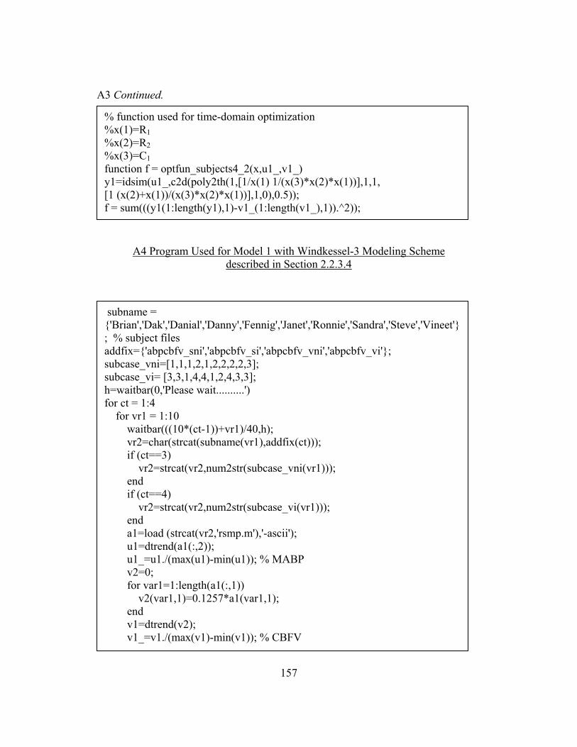
157
A3 Continued.
A4 Program Used for Model 1 with Windkessel-3 Modeling Scheme
described in Section 2.2.3.4
% function used for time-domain optimization %x(1)=R1 %x(2)=R2 %x(3)=C1 function f = optfun_subjects4_2(x,u1_,v1_) y1=idsim(u1_,c2d(poly2th(1,[1/x(1) 1/(x(3)*x(2)*x(1))],1,1, [1 (x(2)+x(1))/(x(3)*x(2)*x(1))],1,0),0.5)); f = sum(((y1(1:length(y1),1)-v1_(1:length(v1_),1)).^2));
subname = {'Brian','Dak','Danial','Danny','Fennig','Janet','Ronnie','Sandra','Steve','Vineet'}; % subject files addfix={'abpcbfv_sni','abpcbfv_si','abpcbfv_vni','abpcbfv_vi'}; subcase_vni=[1,1,1,2,1,2,2,2,2,3]; subcase_vi= [3,3,1,4,4,1,2,4,3,3]; h=waitbar(0,'Please wait..........') for ct = 1:4 for vr1 = 1:10 waitbar(((10*(ct-1))+vr1)/40,h); vr2=char(strcat(subname(vr1),addfix(ct))); if (ct==3) vr2=strcat(vr2,num2str(subcase_vni(vr1))); end if (ct==4) vr2=strcat(vr2,num2str(subcase_vi(vr1))); end a1=load (strcat(vr2,'rsmp.m'),'-ascii'); u1=dtrend(a1(:,2)); u1_=u1./(max(u1)-min(u1)); % MABP v2=0; for var1=1:length(a1(:,1)) v2(var1,1)=0.1257*a1(var1,1); end v1=dtrend(v2); v1_=v1./(max(v1)-min(v1)); % CBFV

158
A4 Continued.
w=hanning(512); Syx=xcorr(v1_,u1_); Sxx=xcorr(u1_); Pmu1 = psd(Sxx,512,2,w,256); Pmv1 = psd(Syx,512,2,w,256); Suf=0; Svf=0; for k=1:length(Pmu1) Suf(k,1)=(Pmu1(k,1))^0.5; Svf(k,1)=(Pmv1(k,1))^0.5; end Z1m1 = Svf./Suf; for var1=1:256 fr(var1,1)=2*(var1/512); % Fs = 2 Hz end Z1m=Z1m1(1:256,1); % measured impedance ctr=1; for wgtime = 0.1:0.1:0.9 % weighting parameter for time MSE wgfreq = 1-wgtime; % weighing parameter for frequency MSE options=optimset('MaxFunEvals',1000000,'MaxIter',1000000,
'TolFun',1.e-1,'TolCon',1.e-1,'TolX',1.e-1); x=0; x=fgoalattain(@freqtime_fun1,[10.6,5.4,3.3],[0,0],
[wgtime,wgfreq],[],[],[],[],[0.01,0.01,0.01],[100,100,100],[], options,u1_,v1_,Z1m);
y2=idsim(u1_,thc2thd(poly2th(1,[1/x(1,1) /(x(1,3)*x(1,2)*x(1,1))],1,1, [1 (x(1,2)+x(1,1))/(x(1,3)*x(1,2)*x(1,1))],1,0),0.5));
mse_tmp1= (sum((y2(1:length(y2),1)- v1_(1:length(v1_),1)).^2))/length(v1_);
if (ctr == 1) mse_tmp2 = mse_tmp1; wg1=[wgtime,wgfreq]; par=[x(1,1) x(1,2) x(1,3)]; elseif (mse_tmp1 < mse_tmp2) mse_tmp2 = mse_tmp1; wg1=[wgtime,wgfreq]; par=[x(1,1) x(1,2) x(1,3)]; end

159
A4 Continued.
ctr=ctr+1; end x=par; y2=idsim(u1_,thc2thd(poly2th(1,[1/x(1,1) 1/(x(1,3)*x(1,2)*x(1,1))],1,1, [1 (x(1,2)+x(1,1))/(x(1,3)*x(1,2)*x(1,1))],1,0),0.5));
mse1=(sum((y2(1:length(y2),1)-v1_(1:length(v1_),1)).^2))/length(v1_); % storing the MSE value for time domain
wg(((ct-1)*10)+vr1,:)=wg1; % storing the weights save(strcat(vr2,'_par.m'),'par','-ascii'); save(strcat(vr2,'_msetimefreq.m'),'mse1','mse2','-ascii'); end end save('weights_1.m','wg','-ascii'); close(h); % function used for optimization %x(1)=R1 %x(2)=R2 %x(3)=C1 function f = freqtime_fun1(x,u1_,v1_,Z1m) for k=1:256 w(k,1) = 2*(k/512); Zw(k,1) = abs((1+i*(w(k,1)*x(3)*x(2)))/(x(2)+x(1) +i*(w(k,1)*x(3)*x(1)*x(2)))); end y1 = idsim(u1_,c2d(poly2th(1,[1/x(1) 1/(x(3)*x(2)*x(1))],1,1,[1 (x(2)+x(1))/(x(3)*x(2)*x(1))],1,0),0.5)); f = [sum(((y1(1:length(y1),1)-v1_(1:length(v1_),1)).^2)), sum((Zw(1:256,1)-Z1m(1:256,1)).^2)];

160
APPENDIX B
COMPARISON OF MSE AND PARAMETER VALUES

161
Table B1 Comparison (t-test) of MSE values of 10 subjects for four data conditions between ARX-2 (1st order model) and Windkessel-1 (Model 1) modeling schemes
SNI SI VNI VI
Pval 0.795561 0.846517 0.528716 0.171701
Table B2 Comparison (t-test) of MSE values of 10 subjects for four data conditions between ARX-2 (2nd order model) and Windkessel-1 (Model 2) modeling schemes
SNI SI VNI VI
Pval 0.035873 0.380281 0.226517 0.343361
Table B3 Comparison (t-test) of MSE values of 10 subjects for four data conditions between ARX-2 (3rd order model) and Windkessel-1 (Model 3) modeling schemes
SNI SI VNI VI
Pval 0.043953 0.423494 0.371526 0.343403
Table B4 Comparison (t-test) of MSE values of 10 subjects for four data conditions between ARX-2 (3rd order model) and Windkessel-1 (Model 4) modeling schemes
SNI SI VNI VI
Pval 0.043953 0.423494 0.371526 0.343403
Table B5 Comparison (t-test) of MSE values of 10 subjects for four data conditions between ARX-2 (2nd order model) and Windkessel-1 (Model 5) modeling schemes
SNI SI VNI VI
Pval 0.009435 0.338753 0.303466 0.343577

162
Table B6 Comparison (t-test) of MSE values of 10 subjects for four data conditions between ARX-2 (1st order model) and Windkessel-2 (Model 1) modeling schemes
SNI SI VNI VI
Pval 0.882653 0.493889 0.537134 0.168465
Table B7 Comparison (t-test) of MSE values of 10 subjects for four data conditions between ARX-2 (2nd order model) and Windkessel-2 (Model 2) modeling schemes
SNI SI VNI VI
Pval 0.017622 0.926783 0.37839 0.342751
Table B8 Comparison (t-test) of MSE values of 10 subjects for four data conditions between ARX-2 (3rd order model) and Windkessel-2 (Model 3) modeling schemes
SNI SI VNI VI
Pval 0.093488 0.876214 0.658093 0.343373
Table B9 Comparison (t-test) of MSE values of 10 subjects for four data conditions between ARX-2 (3rd order model) and Windkessel-2 (Model 4) modeling schemes
SNI SI VNI VI
Pval 0.074718 0.928205 0.821422 0.343388
Table B10 Comparison (t-test) of MSE values of 10 subjects for four data conditions between ARX-2 (2nd order model) and Windkessel-2 (Model 5) modeling schemes
SNI SI VNI VI
Pval 0.036894 0.544073 0.494593 0.342687

163
Table B11 Comparison (t-test) of MSE values of 10 subjects for four data conditions between Windkessel-1 and Windkessel-2 modeling schemes for Model 1
SNI SI VNI VI
Pval 0.68782 0.464833 0.981423 0.805173
Table B12 Comparison (t-test) of MSE values of 10 subjects for four data conditions between Windkessel-1 and Windkessel-2 modeling schemes for Model 2
SNI SI VNI VI
Pval 0.649444 0.425047 0.856225 0.38808
Table B13 Comparison (t-test) of MSE values of 10 subjects for four data conditions between Windkessel-1 and Windkessel-2 modeling schemes for Model 3
SNI SI VNI VI
Pval 0.286579 0.48866 0.541137 0.416529
Table B14 Comparison (t-test) of MSE values of 10 subjects for four data conditions between Windkessel-1 and Windkessel-2 modeling schemes for Model 4
SNI SI VNI VI
Pval 0.193247 0.393005 0.815817 0.542089
Table B15 Comparison (t-test) of MSE values of 10 subjects for four data conditions between Windkessel-1 and Windkessel-2 modeling schemes for Model 5
SNI SI VNI VI
Pval 0.169342 0.691807 0.864143 0.359314
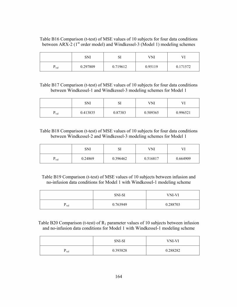
164
Table B16 Comparison (t-test) of MSE values of 10 subjects for four data conditions between ARX-2 (1st order model) and Windkessel-3 (Model 1) modeling schemes
SNI SI VNI VI
Pval 0.297809 0.719612 0.95119 0.171572
Table B17 Comparison (t-test) of MSE values of 10 subjects for four data conditions between Windkessel-1 and Windkessel-3 modeling schemes for Model 1
SNI SI VNI VI
Pval 0.413835 0.87383 0.509365 0.996521
Table B18 Comparison (t-test) of MSE values of 10 subjects for four data conditions between Windkessel-2 and Windkessel-3 modeling schemes for Model 1
SNI SI VNI VI
Pval 0.24869 0.396462 0.516817 0.664909
Table B19 Comparison (t-test) of MSE values of 10 subjects between infusion and no-infusion data conditions for Model 1 with Windkessel-1 modeling scheme
SNI-SI VNI-VI
Pval 0.763949 0.288703
Table B20 Comparison (t-test) of R1 parameter values of 10 subjects between infusion and no-infusion data conditions for Model 1 with Windkessel-1 modeling scheme
SNI-SI VNI-VI
Pval 0.393828 0.288282

165
Table B21 Comparison (t-test) of R2 parameter values of 10 subjects between infusion and no-infusion data conditions for Model 1 with Windkessel-1 modeling scheme
SNI-SI VNI-VI
Pval 0.757161 0.656618
Table B22 Comparison (t-test) of C1 parameter values of 10 subjects between infusion and no-infusion data conditions for Model 1 with Windkessel-1 modeling scheme
SNI-SI VNI-VI
Pval 0.69311 0.681824
Table B23 Comparison (t-test) of MSE values of 10 subjects between infusion and no-infusion data conditions for Model 2 with Windkessel-1 modeling scheme
SNI-SI VNI-VI
Pval 0.730341 0.325159
Table B24 Comparison (t-test) of R1 parameter values of 10 subjects between infusion and no-infusion data conditions for Model 2 with Windkessel-1 modeling scheme
SNI-SI VNI-VI
Pval 0.393828 0.288282
Table B25 Comparison (t-test) of R2 parameter values of 10 subjects between infusion and no-infusion data conditions for Model 2 with Windkessel-1 modeling scheme
SNI-SI VNI-VI
Pval 0.978729 0.153842

166
Table B26 Comparison (t-test) of R3 parameter values of 10 subjects between infusion and no-infusion data conditions for Model 2 with Windkessel-1 modeling scheme
SNI-SI VNI-VI
Pval 0.978581 0.153842
Table B27 Comparison (t-test) of C1 parameter values of 10 subjects between infusion and no-infusion data conditions for Model 2 with Windkessel-1 modeling scheme
SNI-SI VNI-VI
Pval 0.430827 0.727742
Table B28 Comparison (t-test) of C2 parameter values of 10 subjects between infusion and no-infusion data conditions for Model 2 with Windkessel-1 modeling scheme
SNI-SI VNI-VI
Pval 0.430826 0.727007
Table B29 Comparison (t-test) of MSE values of 10 subjects between infusion and no-infusion data conditions for Model 3 with Windkessel-1 modeling scheme
SNI-SI VNI-VI
Pval 0.938366 0.802229
Table B30 Comparison (t-test) of R1 parameter values of 10 subjects between infusion and no-infusion data conditions for Model 3 with Windkessel-1 modeling scheme
SNI-SI VNI-VI
Pval 0.393828 0.288282
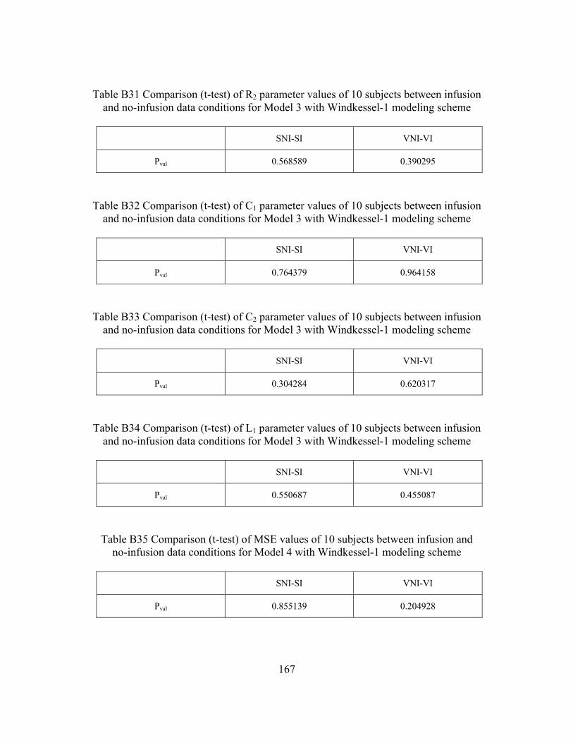
167
Table B31 Comparison (t-test) of R2 parameter values of 10 subjects between infusion and no-infusion data conditions for Model 3 with Windkessel-1 modeling scheme
SNI-SI VNI-VI
Pval 0.568589 0.390295
Table B32 Comparison (t-test) of C1 parameter values of 10 subjects between infusion and no-infusion data conditions for Model 3 with Windkessel-1 modeling scheme
SNI-SI VNI-VI
Pval 0.764379 0.964158
Table B33 Comparison (t-test) of C2 parameter values of 10 subjects between infusion and no-infusion data conditions for Model 3 with Windkessel-1 modeling scheme
SNI-SI VNI-VI
Pval 0.304284 0.620317
Table B34 Comparison (t-test) of L1 parameter values of 10 subjects between infusion and no-infusion data conditions for Model 3 with Windkessel-1 modeling scheme
SNI-SI VNI-VI
Pval 0.550687 0.455087
Table B35 Comparison (t-test) of MSE values of 10 subjects between infusion and no-infusion data conditions for Model 4 with Windkessel-1 modeling scheme
SNI-SI VNI-VI
Pval 0.855139 0.204928

168
Table B36 Comparison (t-test) of R1 parameter values of 10 subjects between infusion and no-infusion data conditions for Model 4 with Windkessel-1 modeling scheme
SNI-SI VNI-VI
Pval 0.393828 0.288282
Table B37 Comparison (t-test) of R2 parameter values of 10 subjects between infusion and no-infusion data conditions for Model 4 with Windkessel-1 modeling scheme
SNI-SI VNI-VI
Pval 0.257989 0.691529
Table B38 Comparison (t-test) of C1 parameter values of 10 subjects between infusion and no-infusion data conditions for Model 4 with Windkessel-1 modeling scheme
SNI-SI VNI-VI
Pval 0.491042 0.52144
Table B39 Comparison (t-test) of C2 parameter values of 10 subjects between infusion and no-infusion data conditions for Model 4 with Windkessel-1 modeling scheme
SNI-SI VNI-VI
Pval 0.310584 0.074284
Table B40 Comparison (t-test) of L1 parameter values of 10 subjects between infusion and no-infusion data conditions for Model 4 with Windkessel-1 modeling scheme
SNI-SI VNI-VI
Pval 0.992003 0.834781

169
Table B41 Comparison (t-test) of MSE values of 10 subjects between infusion and no-infusion data conditions for Model 5 with Windkessel-1 modeling scheme
SNI-SI VNI-VI
Pval 0.12183 0.326871
Table B42 Comparison (t-test) of R1 parameter values of 10 subjects between infusion and no-infusion data conditions for Model 5 with Windkessel-1 modeling scheme
SNI-SI VNI-VI
Pval 0.393828 0.288282
Table B43 Comparison (t-test) of R2 parameter values of 10 subjects between infusion and no-infusion data conditions for Model 5 with Windkessel-1 modeling scheme
SNI-SI VNI-VI
Pval 0.408513 0.710861
Table B44 Comparison (t-test) of C1 parameter values of 10 subjects between infusion and no-infusion data conditions for Model 5 with Windkessel-1 modeling scheme
SNI-SI VNI-VI
Pval 0.634658 0.7375
Table B45 Comparison (t-test) of L1 parameter values of 10 subjects between infusion and no-infusion data conditions for Model 5 with Windkessel-1 modeling scheme
SNI-SI VNI-VI
Pval 0.269113 0.104187

170
Table B46 Comparison (t-test) of MSE values of 10 subjects between infusion and no-infusion data conditions for 1st order model with ARX-2 modeling scheme
SNI-SI VNI-VI
Pval 0.617352 0.163342
Table B47 Comparison (t-test) of a1 parameter values of 10 subjects between infusion and no-infusion data conditions for 1st order model with ARX-2 modeling scheme
SNI-SI VNI-VI
Pval 0.583461 0.203746
Table B48 Comparison (t-test) of b0 parameter values of 10 subjects between infusion and no-infusion data conditions for 1st order model with ARX-2 modeling scheme
SNI-SI VNI-VI
Pval 0.157702 0.01745
Table B49 Comparison (t-test) of b1 parameter values of 10 subjects between infusion and no-infusion data conditions for 1st order model with ARX-2 modeling scheme
SNI-SI VNI-VI
Pval 0.090033 0.034714

171
REFERENCES
1. Ljung L., “System Identification: Theory for the User”, 2nd Edition, Upper
Saddle River, NJ: Prentice Hall PTR, 1999.
2. MATLAB User Manual (Release 13) ver. 6.5, 2002.
3. Stuart Ira Fox, “Human Physiology”, 6th Edition, McGraw-Hill, 1999.
4. Carter GC, Knapp CH, Nuttall AH, “Statistics of the Estimate of the Magnitude-
Coherence Function”, IEEE Transactions on Audio and Electro Acoustics, Vol.
21, no. 4, pp 388-389, 1973.
5. Carter GC, Knapp CH, Nuttall AH, “Estimation of the Magnitude-Squared
Coherence Function via Overlapped Fast Fourier Transform Processing”, IEEE
Transactions on Audio and Electro Acoustics, Vol. 21, no. 4, pp 337-343, 1973.
6. Diehl RR, Linden D, Lücke D, Berlit P, “Phase Relationship between Cerebral
Blood Flow Velocity and Blood Pressure: A Clinical Test of Autoregulation”,
Stroke 26: 1801-1804. 1995.
7. Panerai RB, Chacon M, Pereira R, Evans DH, “Neural Networks Modeling of
Dynamic Cerebral Autoregulation Assessment and Comparison with Established
Methods”, Medical Engineering and Physics Vol. 26, pp 43-52, 2004.
172
8. Panerai RB, Dawson SL, Chacon Potter JF, “Linear and Non-linear Analysis of
Human Dynamic Cerebral Autoregulation”, American Journal of Physiology,
Heart Circulation Physiology, Vol. 277, pp 1089-1099, 1999.
9. Panerai RB, Eames PJ, Potter JF, “Variability of Time-domain Indices of
Dynamic Cerebral Autoregulation”, Physiol. Meas. 24 (2003) 367-381.
10. Panerai RB, “Assessment of Cerebral Pressure Autoregulation in Humans – A
Review of Measurement Methods”, Physiol. Meas. 19 (1998) 305-338.
11. Behbehani K, Zhang R, Peng Q, and Levine BD, “Parametric and Non-
Parametric Modeling of Spontaneous Cerebral Blood Flow Velocity
Variations”, Biomedical Engineering Society 2001 Annual Fall Meeting, Oct. 4-
7, 2001, Annals of Biomedical Engineering Vol. 29, Supplement 1, page S-79
12. Zhang R, Zuckerman JH, Giller CA, Levine BD, “Transfer Function Analysis of
Dynamic Cerebral Autoregulation in Humans”, American Journal of
Physiology, Vol. 274. Heart Circulation Physiology, 43, pp 233-241, 1998.
13. Zhang R, Zuckerman JH, Iwasaki K, Wilson TE, Crandall GC, Levine BD,
“Autonomic Neural Control of Dynamic Cerebral Autoregulation in Humans”,
Circulation. 2002; 106:1814-1820.
14. Zhang R, Behbehani K, Crandall CG, Zuckerman JH, Levine BD, “Dynamic
Regulation of Heart Rate during Acute Hypotension: New Insight into
Baroreflex Function”, American Journal of Physiology, Heart Circulation
Physiology, Vol. 280, pp 407-419, 2001.

173
15. Aaslid R, Lash SR, Bardy GH, Gild WH, Newell DW, “Dynamic Pressure-Flow
Velocity Relationships in Human Cerebral Circulation”, Stroke 2003;34:1645-
1649.
16. Olufsen M, Tran H, Ottesen J, “Modeling Cerebral Blood Flow Control during
Posture Change from Sitting to Standing”, Journal of Cardiovascular
Engineering, Vol. $, No. 1, March 2004.
17. Olufsen M, “On Deriving Lumped Models for Blood Flow and Pressure in the
Systemic Arteries”, Mathematical Biosciences and Engineering, Vol. 1, No. 1,
June 2004.
18. Zhang R, Crandall CG, Levine BD, “Cerebral Hemodynamics During Valsalva
Maneuver: Insights from Ganglion Blockade”, Stroke 2004;35:843-847.
19. Zhang R, Iwasaki K, Zuckerman J, Behbehani K, Crandall CG, Levine BD,
“Mechanism of Blood Pressure and R-R Variability: Insights from Ganglion
Blockade in Humans”, Journal of Physiology, 543.1, pp.337-348,2002.
20. Zhang R, Zuckerman J, Levine BD, “Deterioration of Cerebral Autoregulation
during Orthostatic Stress: Insights from the Frequency Domain”, Journal of
Applied Physiology, 1998.
21. Olufsen M, Nadim A, Lipsitz L, “Autoregulation of Cerebral Blood Flow”,
IEEE Transactions on Biomedical Engineering, 2000.
22. Akaike H, “A New Look at the Statistical Model Identification”, IEEE
Transactions on Automatic Control, December 1974.

174
23. Ursino M, Lodi CA, “A Simple Mathematical Model of the Interaction between
Intracranial Pressure and Cerebral Hemodynamics”, Journal of Applied
Physiology, 1997.
24. Ursino M, Giulioni M, Lodi CA, “Relationships among Cerebral Perfusion
Pressure, Autoregulation, and Transcranial Doppler Waveform: A Modeling
Study”, Journal of Neurosurgery, Vol. 89:255-266, 1998.
25. Dawson SL, Panerai RB, Potter JF, “Critical Closing Pressure Explains Cerebral
Hemodynamics during Valsalva Maneuver”, Journal of Applied Physiology,
1999.
26. Greenfield JC, Rembert JC, Tindall GT, “Transient Changes in Cerebral
Vascular Resistance during the Valsalva Maneuver in Man”, Stroke Vol. 15, No.
1, 1984.
27. Christini DJ, Bennett FM, Lutchen KR, Ahmed HM, Hausdroff JM, Oriol N,
“Application of Linear and Nonlinear Time Series Modeling to Heat Rate
Dynamics Analysis”, IEEE transactions on Biomedical Engineering, Vol. 42,
No. 4, April 1995.
28. Tiecks FP, Douville C, Byrd S, Lam AM, Newell DW, “Evaluation of Impaired
Cerebral Autoregulation by the Valsalva Maneuver”, Stroke 1996;27:1177-
1182.
29. Pott F, Van Lieshout JJ, Ide K, Madsen P, Secher NH, “Middle Cerebral Artery
Blood Velocity during a Valsalva Maneuver in the Standing Position”, Journal
of Applied Physiology, 88:1545-1550,2000.

175
30. Tiecks FP, lam AM, Matta BF, Strebel S, Douville C, Newell Dw, “Effects of
the Valsalva Maneuver on Cerebral Circulation in Healthy Adults”, Stroke,
1995;26:1386-1392.
31. Ling RYS, Clark JW, Srinivasan R, Cole JS, Pruett RC, “An Identification
Scheme for the Determination of Systemic Arterial Load Parameters”, Technical
Report #7507, Department of Electrical Engineering, Rice University, Houston
Texas, U.S.A, April 1975.
32. Mandeville JB, Marota JJ, Ayata C, Zaharchuk G, Moskowitz MA, Rosen BR,
Weisskoff RM, “Evidence of Cerebrovascular Postarteriole Windkessel with
delayed Compliance”, Journal of Cerebral Blood Flow and Metabolism, 19:679-
689, 1999.
33. Segers P, Brimioulle S, Stergiopulos N, Westerhof N, Naeije R, Maggiorini M,
Verdonck P, “Pulmonary Arterial Compliance in Dogs and Pigs: The Three-
Element Windkessel Model revisited”, Journal of Applied Physiology, 1999.
34. Grant BJB, Paradowski J, “Characterization of Pulmonary Arterial Input
Impedance with Lumped Parameter Models”, Journal of Applied Physiology,
1987.
35. Fogliardi R, Donfrancesco MD, Burattini R, “Comparison of Linear and
Nonlinear Formulations of the Three-Element Windkessel Models”, Journal of
Applied Physiology, 1996.

176
36. Zhang S, Finkelstein SM, Cohn JN, “Verification of the Modified Windkessel
Model of the Arterial Vasculature”, IEEE transactions on Biomedical
Engineering, 1992.
37. Manning TS, Shykoff BE, Izzo JL, “Validity and Reliability of Diastolic Pulse
Contour Analysis (Windkessel Model) in Humans”, Hypertension, 2002;
39:963-968.
38. Stergiopulos N, Westerhof BE, Westerhof N, “Total Arterial Inertance as the
Fourth Element of the Windkessel Model”, Journal of Applied Physiology,
1999.
39. Crabtree V, Smith PR, “Physiological Models of the Human Vasculature and
Photoplethysmography”, Electronic Systems and Control Division Research,
2003.
40. McvVeigh GE, Hamilton PK, Morgan DR, “Evaluation of Mechanical Arterial
Properties: Clinical, Experimental and Therapeutic Aspects”, Clinical Science,
2002, 102:51-67.
41. Reinhard M, Roth M, Muller T, Czosnyka M, Timmer J, Hetzel A, “Cerebral
Autoregulation in Carotid Artery Occlusive Disease Assessed From
Spontaneous Blood Pressure Fluctuations by the Correlation Coefficient Index”,
Stroke, 2003;34:2138-2144.

177
42. Novak V, Yang ACC, Lepicovsky L, Goldberger AL, Lipsitz LA, Peng CK,
“Multimodal Pressure-Flow Method to Assess Dynamics of Cerebral
Autoregulation in Stroke and Hypertension”, BioMedical Engineering OnLine
2004, 3:39.
43. Kuo TBJ, Chern CM, Sheng WY, Wong WJ, Hu HH, “Frequency Domain
Analysis of Cerebral Blood Flow Velocity and Its Correlation with Arterial
Blood Pressure”, Journal of Cerebral blood Flow and Metabolism, 1998;18:311-
318.
44. Mathew AM, “Parametric Analysis of Cerebral Autoregulation”, Project Report,
Joint Biomedical Engineering Program, University of Texas at Arlington and
University of Texas Southwestern Medical Center at Dallas, December 2003.
178
BIOGRAPHICAL INFORMATION
Piyush Gehalot was born in Dewas, a small town in Central India, on the 28th of
May, 1980. He received his degree in Bachelor of Engineering in Electronics and
Instrumentation Engineering from Institute of Engineering and Technology (I.E.T.),
Indore, in May 2002. He then decided to pursue his graduate studies in the area of
Biomedical Engineering at the University of Texas at Arlington, specializing in the
track of Bioinstrumentation and Human Performance. His current research interests are
in the area of Physiological System Modeling and Identification, Biomedical Signal
Processing, Process Control and Image Processing. He looks forward to pursue his
career in Biomedical Engineering research and development.