dynamic predictor selection in a new ... - economics.uci.edu

Dynamic predictor selection in a new Keynesian model withheterogeneous expectations$

William A. Branch a,!, Bruce McGough b

a University of California, Irvine, USAb Oregon State University, USA

a r t i c l e i n f o

Article history:Received 13 December 2006Received in revised form24 March 2010Accepted 24 March 2010Available online 2 April 2010

JEL classification:E52E32D83D84

Keywords:Heterogeneous expectationsComplex dynamicsDeterminacyMonetary policy

a b s t r a c t

This paper introduces dynamic predictor selection into a New Keynesian model withheterogeneous expectations and examines its implications for monetary policy. Weextend Branch and McGough (2009) by incorporating endogenous time-varyingpredictor proportions along the lines of Brock and Hommes (1997). We find thatperiodic orbits and complex dynamics may arise even if the model under rationalexpectations has a unique stationary solution. The qualitative nature of the non-lineardynamics turns on the interaction between hawkishness of the government’s policy andthe extrapolative behavior of non-rational agents.

& 2010 Elsevier B.V. All rights reserved.

1. Introduction

Among the standard assumptions of the New Keynesian model is the macroeconomic benchmark of (homogeneous)rational expectations (RE). Recent empirical analysis, however, casts some doubt on this assumption’s validity. Usingsurvey data, Branch (2004, 2007), Carroll (2003), and Mankiw et al. (2003) provide evidence that economic forecasters(both consumers and professional economists) have heterogeneous expectations; and, importantly, the distribution ofheterogeneity evolves over time in response to economic volatility. Branch (2004), in particular, provides evidence thatsurvey respondents in the Michigan survey of consumers are distributed across rational and adaptive expectations andthese proportions evolve over time as a reaction to past mean square forecast errors: for instance, in periods of higheconomic volatility such as the 1970’s a higher proportion of agents used rational expectations than during periods ofrelatively low volatility.

Contents lists available at ScienceDirect

journal homepage: www.elsevier.com/locate/jedc

Journal of Economic Dynamics & Control

ARTICLE IN PRESS

0165-1889/$ - see front matter & 2010 Elsevier B.V. All rights reserved.doi:10.1016/j.jedc.2010.03.012

$ We are grateful to George Evans, Larry Christiano, and Chuck Carlstrom for suggestions. We also thank Fabio Milani and seminar participants at SanFrancisco FRB and Cleveland FRB, and conference participants at Learning Week at the Saint Louis FRB, the Swiss National Bank, the Lorentz Center inLeiden NL, the Society for Computational Economics in Montreal, and the University of Paris X at Nanterre for comments. This paper benefitedsignificantly from the helpful comments of two referees and the Editor.! Corresponding author. Tel.: +19498244221.E-mail address: [email protected] (W.A. Branch).

Journal of Economic Dynamics & Control 34 (2010) 1492–1508

www.elsevier.com/locate/jedc

dx.doi.org/10.1016/j.jedc.2010.03.012

mailto:[email protected]

In light of the empirical evidence, Branch and McGough (2009), relaxing the assumption of rational expectations,incorporate heterogeneous boundedly rational agents into the micro-foundations of a New Keynesian model. The primarycontribution of Branch and McGough (2009) is an aggregation result based on linear approximations to agents’ optimaldecision rules which, themselves, depend on heterogeneous expectations operators. Specifically, under fairly generalassumptions on how agents form expectations, it was shown that aggregate outcomes satisfy IS and AS equations whichhave the same functional form as those in the standard model except that the homogeneous expectations operator isreplaced with a convex combination of heterogeneous expectations operators. This extension of the basic model hasimportant implications for the dynamics of the economy. As a concrete example, Branch and McGough (2009) assumeagents are (exogenously) split between rational and adaptive expectations and monetary policy follows a Taylor-type rule.In this special case, the dynamic properties of the heterogeneous expectations model depend crucially on the distributionof agents across forecasting models and, in particular, its dynamic properties differ from those implied by the standard REmodel.

In Branch and McGough (2009), we took the distribution of heterogeneous expectations as fixed and exogenous. Theempirical evidence cited above and the results from our previous paper, suggest that this assumption is overly restrictive.In this paper, we follow Brock and Hommes (1997) and assume that the degree of heterogeneity is allowed to vary overtime in response to past forecast errors (net of a fixed cost) thereby coupling predictor choice with the dynamics ofinflation and output. As in Brock and Hommes (1997), our predictor choice stems from a discrete choice framework thathas a venerable history in economics, e.g. Manski and McFadden (1981).

The primary interest of this paper is to study the dynamics of a monetary economy with heterogeneous expectationsand dynamic predictor selection. We assume agents choose between using a rational predictor (for a cost) and using anadaptive forecasting model. We find that for sufficiently low costs to using the rational predictor, the model’s steady stateis stable. For higher costs, however, the steady state may destabilize and the dynamic system may bifurcate. Whether thisbifurcation leads to bounded complex dynamics depends on the coefficients in the monetary policy rule and the degree towhich the adaptive agents extrapolate from past data. We find two different cases under which bounded complexdynamics may obtain, depending on the stance of monetary policy: first, if policy is passive, in the sense of adjustingnominal interest rates less than one for one with inflation, or, second, if monetary policy is active and the adaptive agentsextrapolate from past data.

The intuition behind the onset of complicated dynamics in the heterogeneous New Keynesian model may be obtainedas follows. Suppose that agents have a choice of using a rational predictor or an adaptive predictor, and that they seek tominimize their mean square forecast error net of a cost, C, to using the rational predictor. Suppose also that monetarypolicy follows a Taylor-type rule that adheres to the ‘Taylor principle’ by adjusting nominal interest rates more than one forone when inflation deviates from a target. This is the standard advice for setting monetary policy in New Keynesianmodels. As will be evident below, the heterogeneous expectations model with dynamic predictor selection can berepresented as a dynamical system of the form:

xt ¼Mðnt#1Þxt#1;

where x is a vector consisting of aggregate output and inflation, and n is the fraction of rational agents. For n appropriatelylarge, but less than one, the eigenvalues of M lie inside the unit circle. Now consider what happens to an economy thatbegins with a fraction of rational agents close to one. Since the eigenvalues of M will have modulus less than one, theeconomy will contract toward the steady state and the relative advantage of rational over adaptive expectations willdiminish. As a result, a growing proportion of agents will not want to pay the fixed cost to being rational. The proportion ofrational agents n will decrease until an eigenvalue of M again has modulus greater than one, causing the economy to repelfrom the steady state. This attracting/repelling feature of dynamic predictor selection is what makes bounded complexdynamics exist even in the case that monetary policy adheres to the Taylor principle.1

The potential for complex dynamics have important implications for monetary policy. A wide and established literatureappears to agree on one essential ingredient of sound monetary policy: policy should be set to act aggressively againstinflation (e.g. Taylor, 1999; Clarida et al., 2000; Bernanke and Woodford, 1997; Svensson and Woodford, 2003; Woodford,2003). A basis for this finding is that adherence to an active monetary policy rule (a variant on the ‘Taylor principle’) resultsin a determinate model and thus a unique rational expectations equilibrium.2 However, in the case of heterogeneousexpectations, we find that even an active rule may result in complex behavior and thus possibly excess volatility. In fact,not only does the interaction between monetary policy and expectations formation in part dictate the ensuing dynamicbehavior, we even find that these complicated dynamics may arise when monetary policy is set to guarantee determinacyunder rational expectations. To most convincingly illustrate this point, we specify a policy rule that yields determinacyunder RE, and we assume that there is a fixed cost to deviating from rational expectations—precisely the setting assumedfor, and implied by, standard monetary policy advice: even in this case the economy may exhibit bounded complexdynamics. Our results suggest that, in the presence of heterogeneous agents, determinacy under RE may not be a robustcriterion for policy advice. The complex dynamics produced by our model are not outcomes limited to unusual calibrations

ARTICLE IN PRESS

1 This intuition for switching between stable and unstable dynamics was first discovered in a cobweb model by Brock and Hommes (1997).2 A determinate model is sometimes called ‘‘stable’’ because, due to its unique equilibrium, the economy is not subject to excessive volatility that can

arise when agents’ beliefs are driven by self-fulfilling prophecies (e.g. sunspots).

W.A. Branch, B. McGough / Journal of Economic Dynamics & Control 34 (2010) 1492–1508 1493

or a priori poor policy choices: complex behavior appears to be an almost ubiquitous feature of a time-varyingheterogeneous expectations New Keynesian model.

That determinacy of a steady state may not be sufficient to guard against instability has been demonstrated elsewhere.Benhabib et al. (2001) show that a determinate steady state may be surrounded by bounded complex dynamics whennominal interest rates have a zero lower bound, even under the assumption of rationality. Benhabib and Eusepi (2004)conclude that a New Keynesian model extended to include capital may possess chaotic dynamics. Bullard and Mitra (2002)show that determinacy is neither necessary nor sufficient for a rational expectations equilibrium to be stable underadaptive learning. Gali et al. (2004) derive a model with a proportion of rule of thumb consumers and demonstrate that thedeterminacy properties of the model are sensitive to the presence of these agents. Levin and Williams (2003) stress theimportance of policy being robust across potential model specifications. DeGrauwe (2008) studies how heterogeneity andmonetary policy can interact to lead to endogenous dynamics. Finally, Anufriev et al. (2009) demonstrate that in a stylizedmacro model with heterogeneous expectations multiple steady states may arise even when the Taylor principle holds.

This paper is organized as follows. Section 2 presents an overview of the New Keynesian model with heterogeneousexpectations and introduces dynamic predictor selection into the model. Section 3 presents the analysis and results whileSection 4 concludes.

2. A new Keynesian model with heterogeneous expectations

In Branch and McGough (2009), we derive a New Keynesian model with heterogeneous expectations where aggregateoutput and inflation are governed by the following equations

yt ¼ Etytþ1#s#1ðit#Etptþ1Þ ð1Þ

pt ¼ bEtptþ1þlyt : ð2Þ

Here yt is aggregate output gap, pt is the inflation rate, and Et is a heterogeneous expectations operator defined as a convexcombination of boundedly rational (and possibly rational) forecasting models. Below we make explicit assumptions on E.Note that under rational expectations, i.e. E ¼ E, the unique steady state for the economy is y¼ p¼ 0.

The form of (1)–(2) is a New Keynesian model in which conditional expectations have been replaced by a heterogeneousexpectations operator Et . Branch and McGough (2009) derive these reduced-form equations from linear approximations tothe optimal decision rules in a Yeoman-farmer economy extended to include two types of agents, differing in theirforecasting mechanism. The first Eq. (1) represents the demand side of the economy. Under homogeneous expectations, itis derived as a log-linear approximation to the representative agent’s Euler equation. With heterogeneous agents, the ISequation (1) is found by aggregating the Euler equations across heterogeneous agents. The parameter s#1 is the usual realinterest elasticity of output.

The second Eq. (2) is the aggregate supply relation. Similar to the representative agent model, it is found by averagingthe pricing decisions of firms in the economy. In this formulation, l is the usual measure of output elasticity of inflation.The functional forms of these IS–AS relations are the same as those in the standard New Keynesian model. The keydistinction is that because of the heterogeneity in beliefs, the equilibrium processes for aggregate output and inflationdepend on the distribution of agents’ expectations. In Branch and McGough (2009), we provide the axiomatic foundationsthat facilitate aggregating heterogeneous expectations into the tractable reduced form (1)–(2). This paper takes as giventhat these are the equations governing the economy and studies the dynamic implications of heterogeneous expectations.We remark, however, that the form of heterogeneity assumed in this paper is consistent with the theoretical foundations inBranch and McGough (2009).

We assume that monetary policy is specified by the following instrument rule:

it ¼ ayEtytþ1þapEtptþ1: ð3Þ

The form of (3) is what Evans and Honkapohja (2005), Evans and McGough (2005a,b), and Preston (2005b) call an‘expectations-based’ rule. It is a simple implementable rule that takes advantage of a policymakers’ observations of privatesector expectations, and follows Bernanke (2004) in advocating for a policy that reacts aggressively to private-sectorexpectations. Implementation of such a rule is straightforward, even in an economy with heterogeneous agents, so long asthe average forecast is observed by policymakers. In practice, this is a reasonable assumption as there are many market andsurvey based measures of the average, or consensus, inflation and output forecasts. None of the qualitative results in thispaper, however, are sensitive to the form of the nominal interest rate targeting rule. To verify robustness we alsoconsidered a policy rule in which the government sets the instrument against the optimal forecasts of inflation and output,rather than the average of the agents’ forecasts.3 All qualitative results are robust to the alternate form of the instrumentrule.

ARTICLE IN PRESS

3 Here, by ‘‘optimal forecasts,’’ we mean forecasts that minimize mean square error. Because we are in a non-stochastic environment (and we are notconsidering the possibility of associated stochastic sunspot equilibria) optimal forecasts in our model correspond to agents having one-step ahead perfectforesight. These issues are more carefully addressed in Section 2.1 below.

W.A. Branch, B. McGough / Journal of Economic Dynamics & Control 34 (2010) 1492–15081494

Policy rules with forms similar to (3) are often described as Taylor-type instrument rules. These rules are said to satisfythe Taylor principle if the response of nominal interest rates to the inflation metric is greater than one, i.e. ap41. Thisensures that when the central bank adjusts the nominal interest rate it is also adjusting the real interest rate in the samedirection. Below we will find that the qualitative features of the model’s dynamics hinge on whether the policy rulesatisfies the Taylor principle.

2.1. Expectations and predictor dynamics

To close the model we must specify the operator Et . For simplicity, we assume there are precisely two types ofpredictors available to agents: the type 1 predictor, which is called ‘‘rational,’’ and the type 2 predictor, which is called‘‘adaptive.’’ Agents using type 1 predictors are assumed to be very good forecasters, which we capture by providing themperfect foresight when forming one-step-ahead forecasts (and this is why we call them ‘‘rational’’): if x=y or p then Et

1

xt+1=xt+1.4 Agents using type 2 predictors are accessing a less sophisticated technology, and are assumed to look

backwards when forming forecasts (which is why we call them adaptive): if x=y or p then E2t xtþ1 ¼ y2xxt#1; this formulationis derived from a linear forecast rule of the form xt ¼ yxxt#1. Finally, we may set

Etxtþ1 ¼ nxtxtþ1þð1#nxtÞy2xxt#1; ð4Þ

where nxt is the fraction of agents using rational predictors at time t. More details about the construction of theexpectations operator Et may be found in Branch and McGough (2009).

The form of heterogeneous expectations in (4) imposes that agents are heterogeneous in their forecasting of a particularaggregate outcome, rather than heterogeneous in their forecasts related to consumption (i.e. the IS equation) versus pricingbehavior (i.e. the AS equation). This assumption is consistent with the learning literature which models boundedly rationalagents as econometric forecasters attempting to forecast aggregate output and inflation. That agents might want adifferent forecasting model for inflation and output is in line with the findings of Branch and Evans (2006) who computesimple recursive forecasting models that are consistent with survey data on inflation and output expectations. However,the assumption is still somewhat ad hoc and we checked that our qualitative results were robust to imposing theheterogeneity in forecasting methods across IS–AS relations.

We call agents using type 1 predictors rational because they minimize their mean square forecast error. On the otherhand, our agents make time t decisions based only on forecasts of time t+1 aggregate data, and in particular are not ex-anteconcerned with meeting transversality conditions. In the sequel, we focus on equilibrium dynamics that remain uniformlybounded to remain consistent with agents’ transversality conditions ex-post.5 In this way we are modeling our type 1agents in a manner similar to Euler equation learning—a common approach in the learning literature, particularly in thecontext of New Keynesian monetary models: See Evans et al. (2003) for further discussion. The Euler equation approachdictates that households’ decisions satisfy their ex ante first-order optimality conditions and only satisfy the transversalityconditions ex post. In a sense, then, our perfect foresight agents are really good myopic forecasters. An interestingalternative that explicitly accounts for infinite horizon planning is developed by Preston (2005a), and it would be quitenatural to reconsider the questions addressed here using a model consistent with his method.

Agents with type 2 predictors use a fairly standard form of adaptive expectations. Such expectations can be thought ofas arising from a simple linear perceived law of motion of the form xt ¼ yxxt#1. In many models, real-time estimates of yxconverge to their REE minimal state variable (MSV) values. Here we take y as fixed, though an extension with real-timelearning and dynamic predictor selection is a topic of current research.6

When yo1 adaptive agents dampen past data in forming expectations; when y41 agents have extrapolativeexpectations. Adaptive expectations of this form were assumed in Branch and McGough (2009) as well as in Brock andHommes (1997, 1998), Branch (2002), Branch and McGough (2005), and Pesaran (1987). When y¼ 1 the adaptive predictoris usually called ‘naive’ expectations, and was the case emphasized by Brock and Hommes (1997). The y41 case was givenparticular emphasis by Brock and Hommes (1998). It is straightforward to extend the adaptive predictor to incorporatemore lags. We anticipate that such an extension would not alter the qualitative results of this paper but would alter thequantitative details. Despite this simple form of adaptive expectations there is evidence in survey data that agents aredistributed across rational expectations and a simple univariate forecasting model (see Branch, 2004). The contribution ofthis paper is to demonstrate in a simple monetary model that time-varying, endogenously determined distributions ofheterogeneous expectations may significantly alter the equilibrium implications for a given monetary policy.

Having specified the predictors available to agents, it remains to determine the proportion of agents using a particularpredictor. There is growing empirical evidence that the distribution of agents’ heterogeneity is time-varying. For example,Mankiw et al. (2003) study various surveys of inflation expectations and show a wide, time-varying dispersion in beliefs.Branch (2004, 2007) documents time-varying distributions of agents across discrete predictors. In each case, the nature of

ARTICLE IN PRESS

4 This is the version of rationality studied by Brock and Hommes (1997); we employ it here to approximate the notion that rational agents willminimize mean square forecast errors.

5 As we remark below, for some parametric specifications, the equilibrium dynamics do not remain uniformly bounded.6 Branch and Evans (2006) and Guse (2008) have made some progress on this issue.


the variation in the distributions appears structural: in Branch (2004, 2007) volatility causes more agents to adopt rationalexpectations, and in Mankiw et al. (2003) volatility causes dispersion to shrink. Given that the results from Branch andMcGough (2009) suggest that the dynamic properties of the economy are highly sensitive to the fraction of rational agents,and given that there is empirical evidence of time-varying fractions, we turn to an endogenous dynamic predictor selectionversion of the heterogeneous expectations model.7

With dynamic predictor selection nxt ,x¼ y,p are assumed to follow:

nxt ¼exp½oUx

jt 'exp½oUx

jt 'þexp½oUxj0t'

j0aj: ð5Þ

Here Uxjt is a predictor fitness measure to be specified below. This is a multinomial logit law of motion and was employed

by Brock and Hommes (1997), and then extended to a stochastic setting by Branch and Evans (2006). The parameter o iscalled the ‘intensity of choice’; it governs how strongly agents react to past forecast errors. Brock and de Fountnouvelle(2000) and Brazier et al. (2008) adopt a discrete choice setting in monetary models. Brazier et al., assume that oo1proxies for measurement error in calculating forecast errors. In this setting, o is inversely related to the variance of thoseerrors.8

Brock and Hommes (1997), who develop their notion of predictor selection in the context of a univariate linear cobwebmodel, show that for large, but finite, values of o there may exist complex dynamics. The intuition for their finding is thatthe dynamic predictor selection coupled with the equilibrium price dynamics creates a tension between repelling andattracting dynamics. As we will explore in detail below, our analysis of the heterogeneous New Keynesian model with fixedpredictor proportions indicates that the steady state may be dynamically unstable for low values of n and dynamicallystable for large values of n; this creates precisely the sort of repelling/attracting forces that makes bounded, complexdynamics possible.

Since we are modeling the predictor selection as independent of the optimization problem, we assume that predictorsuccess is measured in terms of mean-square error:

MSExjt ¼MSExjt#1þm xt#Ej

t#1xt! "2

#MSExjt#1

# $:

The predictor fitness metric is assumed to be

Uxjt ¼#MSExjt#Cj: ð6Þ

Below, in our numerical simulations we will assume that m¼ 1, so that agents react to last period’s squared error only.9 Wemake this assumption to minimize the number of bifurcation parameters.10 Notice that we also assume a constant in thestatistical metric function Ujt. This constant can be interpreted as the cost of using a particular predictor, or as Branch(2004) emphasizes, as a predisposition effect. Regardless of the interpretation we are not going to a priori impose ahierarchy on the Cj, and instead will treat them as bifurcation parameters. For simplicity, we set the cost of adaptiveexpectations equal to zero, so that C will always represent the relative cost of rationality. Because both adaptive andperfect foresight return the same forecast in a steady state, the value of oC pins down the steady-state value of n, andthereby determines the local stability properties of the model.

We also assume C,o are identical across forecasting variable. This may seem inconsistent with the assumption thatyy,yp may differ. The approach here is flexible enough that we could expand the parameter space and consider the effectsof altering the variable-specific C,o as bifurcation parameters. We leave such an examination to future research. We do notimpose that predictor proportions are identical, and the dynamics of predictor selection will be different for each nx along areal-time path.

The predictor fitness metric may seem somewhat ad-hoc given the micro foundations of the model. We justify the formof (6) by appealing to the learning literature which models expectation formation as a distinct statistical problem. Thus,agents choose a forecasting model based on past success and then use that model to solve for their optimal plan in theanticipated utility sense. This is not difficult to justify since we constructed the agents’ problem so that they are forecastingaggregate variables over which they exert no control.

ARTICLE IN PRESS

7 The importance of endogenous predictor selection and macroeconomic dynamics were also shown by Marcet and Nicolini (2003), Tuinstra andWagener (2007).

8 In our simulations below, we initialize the model in an REE. In the ‘neoclassical’ limit, i.e. o-1, the model will remain in an REE. Thus, thisapproach yields heterogeneity for oo1, so the existence of adaptive agents is a natural consequence of these measurement errors or random utilityterms. In a sense, heterogeneity arises because of some uncertainty about the best forecasting model. In Branch and Evans (2006), heterogeneity arises, ina stochastic univariate model, even as o-1, and we would expect similar results if we extended that framework to a New Keynesian model.

9 The weight m could be treated as a bifurcation parameter: see, for example, Brock et al. (2006).10 Branch and Evans (2006) show that, in a cobweb model, similar results obtain provided m is somewhat close to one. A larger value of m can be

justified if agents are concerned about structural change or uncertain about the right predictor to adopt.


2.2. The dynamic system

With dynamic predictor selection, the economy’s law of motion becomes,

yt ¼ nyt#1ytþ1þð1#nyt#1Þy2yyt#1#s#1ðit#ðnpt#1ptþ1þð1#npt#1Þy

2ppt#1ÞÞ

pt ¼ lytþbðnpt#1ptþ1þð1#npt#1Þy2ppt#1Þ

it ¼ ayðnyt#1ytþ1þð1#nyt#1Þy2yyt#1Þþapðnpt#1ptþ1þð1#npt#1Þy2ppt#1Þ: ð7Þ

The laws of motion for nyt ,npt are specified below.The timing assumptions require special discussion. We follow the adaptive learning literature in assuming that current

values of the endogenous state variables are not directly observable. This is usually assumed to avoid a simultaneity inleast-squares parameter estimates and the endogenous variables. In this setting, the assumption preserves logicalconsistency for adaptive agents. Rational agents (who have one-step-ahead perfect foresight) know current values of allvariables, but the adaptive agents do not. Under this natural assumption, predictor selection takes place at time t#1. Theapproach taken here assumes that agents have a menu of predictor choices, they look at their most recent past forecastingperformance as of the end of the period t#1, and choose the predictor with which they forecast one-step-ahead xt ,pt .These choices then aggregate into nt#1 upon which the current state variables depend.

As noted in the previous section, fully rational agents would be aware of the future evolution of predictor proportions.Obtaining this information and incorporating it into decision-making is a complicated problem and motivates theliterature’s assumption that agents treat the forecasting, or predictor selection, issue as a statistical problem distinct fromtheir optimization. In the current setting, given nt#1, agents behave to satisfy their current Euler equation and currentoptimal pricing equation, and ignore the time-varying nature of the predictor proportions.11 A similar assumptionmotivates the Euler-equation approach of Evans et al. (2003), Bullard and Mitra (2002), and to which Preston (2005a) is analternative. We stay consistent with the Euler-equation approach with the difference here being that the time evolution ofbeliefs is via a pair of fixed predictors while in the adaptive learning models the expectation operators are time varying.These assumptions justify working with the conditionally linear IS and AS Eqs. (1) and (2).

To study the model’s dynamics, impose the policy rule into the IS relation in (7) and simplify to get

Hxt ¼ Fðnt#1Þxtþ1þGðnt#1Þxt#1; ð8Þ

where x¼ ðy,pÞ0, n¼ ðny,npÞ0, and

FðntÞ ¼nytð1#s#1ayÞ s#1ð1#apÞnpt

0 bnpt

!

GðntÞ ¼ð1#nytÞð1#s#1ayÞy2y s-1ðnpt#1Þðap#1Þy2p

0 bð1#nptÞy2p

0

@

1

A

H¼1 0

#l 1

# $: ð9Þ

Now let z¼ ðx0,x0#1Þ0. Since F is generically invertible, we may write

Mðnt ; xÞ ¼FðntÞ-1H #FðntÞ-1GðntÞ

I2 02

!;

where x is the vector of model parameters. Finally, set

f ðzt ;nt ; xÞ ¼expð#oCÞfexpð#oCÞþexp½#oððe01Mðnt ; xÞ#y2ye03ÞztÞ

2'g-1

expð#oCÞfexpð#oCÞþexp½#oððe02Mðnt ,xÞ#y2pe04ÞztÞ2'g-1

0

@

1

A

where ei is the i th coordinate vector. Then the full dynamic system is

zt ¼Mðnt#1;xÞzt#1 ð10Þ

nt ¼ f ðzt#1;nt#1; xÞ: ð11Þ

Given initial conditions z#1 and n#1, the system (10) and (11) determines the evolution of our economy.

ARTICLE IN PRESS

11 Importantly, by behaving in a manner that satisfies the Euler equation, but not the ex ante transversality condition, the perfect foresight agents’beliefs do not make choices so that the economy is necessarily on the stable saddle path associated to the model with fixed predictor proportions.


3. Results

We now present results for the dynamical system (10) and (11). Because the state vector has six dimensions, analyticresults are largely intractable.12 In what follows, we provide a thorough numerical analysis.

3.1. Local stability analysis

The system (10) and (11) always has a steady state given by

z¼ 0 and ny ¼ np ¼expð#oCÞ

expð#oCÞþ1: ð12Þ

We call this the ‘‘zero steady state,’’ and note that the values of inflation and output correspond to the unique rationalexpectations equilibrium in case all agents are rational and the associated RE-model is determinate.

There also may exist steady states in which inflation and output are non-zero. When there exists a non-zero steadystate, y,p, then the steady-state values for ny,np are

ny ¼expð#oCÞ

expð#oCÞþexpð#oð1þyyÞ2y2Þ

np ¼expð#oCÞ

expð#oCÞþexpð#oð1þypÞ2p2Þ:

Notice that in a non-zero steady state, adaptive agents make persistent forecasting errors, but because of the cost C toperfect foresight, they may still prefer the adaptive predictor.

The Jacobian of the dynamic system evaluated at the zero steady state is given by

J¼Mðn; xÞ 0

fzð0;n; xÞ 0

!;

where n is given by (12). Thus the zero steady state’s stability properties are determined by the properties of Mðn,xÞ.Furthermore, the time t dynamics of zt are governed by the eigenvalues of Mðnt#1,xÞ; so to gain intuition about both localstability and other dynamic properties of the model, we turn to the numerical analysis of the matrix M(n).

The properties of MðnÞ, and hence the stability of the dynamical system, depend in a critical way on the steady-statefraction of perfect foresight agents. The tension between the forward-looking expectations of rational agents and thebackward-looking adaptive agents is at the crux of the results to be presented below, and MðnÞ captures the mix of thistension. We can anticipate the results below by first assuming yy ¼ yp ¼ 1 and restricting attention to the two boundarycases:

1. The purely rational steady state, corresponding to C-#1 and n ¼ 1, with equilibrium dynamics given by xt=F(1)#1

Hxt#1;2. The purely adaptive steady state,13 corresponding to C-1 and n ¼ 0, with equilibrium dynamics given by xt=H

#1 G(0)xt#1.

Noting that G(0)=F(1), we have the following result:

Proposition 1. Assume yy ¼ yp ¼ 1. If the purely adaptive steady state is locally stable then the purely rational steady state isunstable. Conversely, if the purely rational steady state is stable, then the purely adaptive steady state is unstable.

The key insight provided by this result is the evidenced tension between the forward and backward looking dynamicsinherent to the heterogeneous expectations model: in the special case of naive expectations, i.e. y¼ 1, if the rationaldynamics are attracting then the adaptive dynamics are repelling, and vice-versa. To gain further intuition about both localstability and other dynamic properties of the model, we turn to the numerical analysis of the matrix M(n).

To conduct our numerical analysis, the model must be calibrated. Table 1 details the parameter constellations for the ISand AS relations: see Woodford (1999), Clarida et al. (2000), Evans and McGough (2005a) and McCallum and Nelson(1999). As in Branch and McGough (2009), all broad qualitative results are robust to the calibration employed.

Completing our numerical specification requires choosing values for yy and yp and our work in Branch and McGough(2009) indicates that the size of these values relative to one impacts the dependence of the model’s dynamic properties onpredictor proportions. To account for the possible impact the magnitude of yx might have on the dynamics of our model,we consider both yx41 and yxo1. For simplicity, we assume yp ¼ yy.

ARTICLE IN PRESS

12 The state vector consists of the (4(1) vector z and the (2(1) vector n.13 As noted above, F(n) is invertible for n 2 ð0,1'. As n-0, detðFÞ-0 so that M becomes undefined. The equilibrium dynamics, in this case, are

obtained via (8).


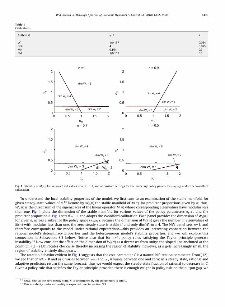
To understand the local stability properties of the model, we first turn to an examination of the stable manifold, forgiven steady-state values of n.14 Denote by Ws(n) the stable manifold of M(n), for predictor proportions given by n; thus,Ws(n) is the direct sum of the eigenspaces of the linear operator M(n) whose corresponding eigenvalues have modulus lessthan one. Fig. 1 plots the dimension of the stable manifold for various values of the policy parameters ay,ap and thepredictor proportion n. Fig. 1 sets y¼ 1:1 and adopts the Woodford calibration. Each panel provides the dimension ofWs(n),for given n, across a subset of the policy space ðap,ayÞ. Because the dimension of Ws(n) gives the number of eigenvalues ofM(n) with modulus less than one, the zero steady state is stable if and only dimWsðnÞ ¼ 4. The NW panel sets n=1, andtherefore corresponds to the model under rational expectations—this provides an interesting connection between therational model’s determinacy properties and the heterogeneous model’s stability properties, and we will explore thisconnection in Subsection 3.3 below. Notice also that for n=1, policy rules satisfying the Taylor principle generateinstability.15 Now consider the effect on the dimension of Ws(n) as n decreases from unity: the sloped line anchored at thepoint ðap,ayÞ ¼ ð1,0Þ rotates clockwise thereby increasing the region of stability; however, as n gets increasingly small, theregion of stability entirely disappears.

The rotation behavior evident in Fig. 1 suggests that the cost parameter C is a natural bifurcation parameter. From (12),we see that @n=@Co0 and as C varies between #1 and 1, n varies between one and zero: in a steady state, rational andadaptive predictors return the same forecast; thus we would expect the steady-state fraction of rational to decrease in C.Given a policy rule that satisfies the Taylor principle, provided there is enough weight in policy rule on the output gap, we

ARTICLE IN PRESS

0 1 20

0.5

1

1.5

2n = 1

α y

0 1 20

0.5

1

1.5

2n = 0.9

α y

0 1 20

0.5

1

1.5

2n = 0.7

απ

α y

0 1 20

0.5

1

1.5

2n = 0.5

α y

dim Ws = 3

dim Ws = 3

dim Ws = 3

dim Ws = 2

dim Ws = 0

dim Ws = 1

dim Ws = 4

dim Ws = 3

dim Ws = 2

dim Ws = 4

dim Ws = 3 dim Ws = 2

dim Ws = 4

dim Ws = 3

dim Ws = 2

0.5απ

1.5

0.5 1.5απ

0.5 1.5

απ

0.5 1.5

Fig. 1. Stability of M(n), for various fixed values of n, y¼ 1:1, and alternative settings for the monetary policy parameters ðap ,ayÞ under the Woodfordcalibration.

Table 1Calibrations.

Author(s) s#1 l

W 1/0.157 0.024CGG 4 0.075MN 0.164 0.3EM 1/0.157 0.3

14 Recall that at the zero steady state, n is determined by the parameters o and C.15 This instability under rationality is expected: see Subsection 3.3.


can choose C so that the zero steady state is stable. For example, in the NE panel, there is a wedge of the upper left quadrantwith ap41 and dimWsðnÞ ¼ 4. By further increasing C, we lower the zero steady-state value n, causing the anchored line torotate clockwise so that the zero steady state destabilizes. When this happens a bifurcation occurs.

The bottom two panels of Fig. 1 indicate a change in the eigenvalue structure of M that is not captured by the rotationalbehavior of the sloped line anchored at the point ðap,ayÞ ¼ ð1,0Þ. Consider the policy rule determined by ap ¼ 1:1, ay ¼ 0:35,as indicated by the circles in the bottom two panels. As n decreases, the dimension of the stable manifold changes fromfour to zero so that the associated steady state destabilizes. Close examination reveals that the bifurcation marking thedestabilization of the steady state is characterized by the simultaneous passage of all four (complex) eigenvalues of Macross the unit circle. The nature of this bifurcation can also be seen from Fig. 4, which is drawn using the policy ruleap ¼ 1:1, ay ¼ 0:35. As noted above, increasing C corresponds to decreasing n. Now follow a horizontal line anchored aty¼ 1:1: as C increases past )#0:19, the eigenvalues simultaneously cross the unit circle (see also footnote 17).

Fig. 2 plots the dimWsðnÞ under the same conditions except that y¼ 0:9. Here we find that the sloped line anchored atðap,ayÞ ¼ ð1,0Þ rotates counterclockwise thereby decreasing the stability region. In this case, rules satisfying the Taylorprinciple will not yield stability, as there is not a part of the policy space where ap41 and dimWsðnÞ ¼ 4. However, certainpassive rules, i.e. apo1, lead to local stability of the zero steady state for large n, as is evident in the top two panels. As Cincreases and n falls, the region of stability will disappear, so that, again, C is a natural bifurcation parameter.

Figs. 1 and 2 suggest that heterogeneity can increase the region of the parameter space that is stable when y41 ordecrease the region for yo1. That y41 can be stabilizing is intuitive. For moderately-sized values of n, y41 works tooffset the unstable forward dynamics from the rational agents. However, for n sufficiently small, e.g. n=0.5, theextrapolative behavior of agents is explosive.

3.2. Simulations and bifurcations

The panels in Figs. 1 and 2 suggest that, for appropriate policy parameters, small values of C will imply that the zerosteady state is locally stable, while increases in C will lead to bifurcation. It may be possible to characterize the primarybifurcation by applying the center manifold reduction technique, though the daunting nature of this task compels us toproceed numerically.16 For a given calibration, value of y, and setting o¼ 1, we choose C so that the zero steady state is

ARTICLE IN PRESS

0.5 1 1.5 2

0.5

1

1.5

2n = 1

απ

α y

1 2

0.5

1

1.5

2n = 0.9

απ

α y

1 2

0.5

1

1.5

2

α y

1 2

1

2

α y



dim Ws = 3


dim Ws = 2


dim Ws = 4

dim Ws = 4

dim Ws = 3

n = 0.8

0.5 1.5

n = 0.6

0.5απ

1.5

1.5

0.5

απ

0.5 1.5

Fig. 2. Stability of M(n), for various fixed values of n, y¼ 0:9, and alternative settings for the monetary policy parameters ðap ,ayÞ under the Woodfordcalibration.

16 For more information on bifurcation theory, see Kuznetsov (1998), Guckenheimer and Holmes (1983), and Palis and Takens (1993).


stable; then, we consider larger values of C and for each new value of C the model is simulated by choosing initialconditions at random near the zero steady state. The first 10,000 periods of transient dynamics are discarded, so that theremaining data will be near the invariant attractor. We then plot these simulations in a bifurcation diagram and in phasespace.

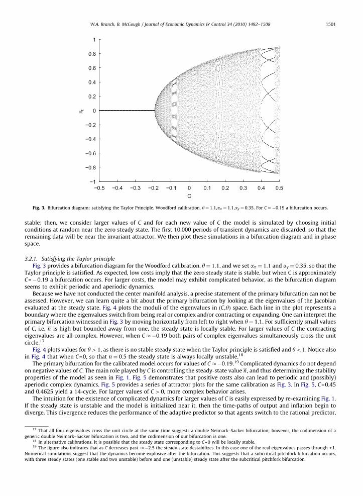
3.2.1. Satisfying the Taylor principleFig. 3 provides a bifurcation diagram for the Woodford calibration, y¼ 1:1, and we set ap ¼ 1:1 and ay ¼ 0:35, so that the

Taylor principle is satisfied. As expected, low costs imply that the zero steady state is stable, but when C is approximatelyC=#0.19 a bifurcation occurs. For larger costs, the model may exhibit complicated behavior, as the bifurcation diagramseems to exhibit periodic and aperiodic dynamics.

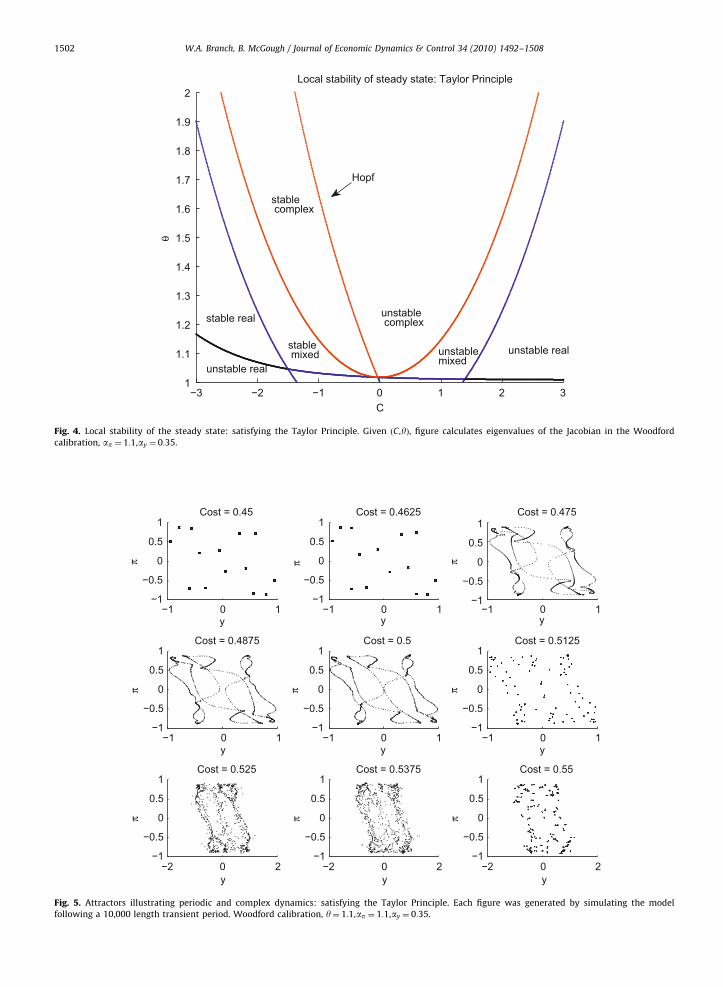
Because we have not conducted the center manifold analysis, a precise statement of the primary bifurcation can not beassessed. However, we can learn quite a bit about the primary bifurcation by looking at the eigenvalues of the Jacobianevaluated at the steady state. Fig. 4 plots the moduli of the eigenvalues in ðC,yÞ space. Each line in the plot represents aboundary where the eigenvalues switch from being real or complex and/or contracting or expanding. One can interpret theprimary bifurcation witnessed in Fig. 3 by moving horizontally from left to right when y¼ 1:1. For sufficiently small valuesof C, i.e. n is high but bounded away from one, the steady state is locally stable. For larger values of C the contractingeigenvalues are all complex. However, when C )#0:19 both pairs of complex eigenvalues simultaneously cross the unitcircle.17

Fig. 4 plots values for y41, as there is no stable steady state when the Taylor principle is satisfied and yo1. Notice alsoin Fig. 4 that when C=0, so that n ¼ 0:5 the steady state is always locally unstable.18

The primary bifurcation for the calibrated model occurs for values of C )#0:19.19 Complicated dynamics do not dependon negative values of C. The main role played by C is controlling the steady-state value n, and thus determining the stabilityproperties of the model as seen in Fig. 1. Fig. 5 demonstrates that positive costs also can lead to periodic and (possibly)aperiodic complex dynamics. Fig. 5 provides a series of attractor plots for the same calibration as Fig. 3. In Fig. 5, C=0.45and 0.4625 yield a 14-cycle. For larger values of C40, more complex behavior arises.

The intuition for the existence of complicated dynamics for larger values of C is easily expressed by re-examining Fig. 1.If the steady state is unstable and the model is initialized near it, then the time-paths of output and inflation begin todiverge. This divergence reduces the performance of the adaptive predictor so that agents switch to the rational predictor,

ARTICLE IN PRESS

0−1

−0.8

−0.6

−0.4

−0.2

0

0.2

0.4

0.6

0.8

1

C

π t

−0.5 −0.4 −0.3 −0.2 −0.1 0.1 0.2 0.3 0.4 0.5

Fig. 3. Bifurcation diagram: satisfying the Taylor Principle. Woodford calibration, y¼ 1:1,ap ¼ 1:1,ay ¼ 0:35. For C )#0:19 a bifurcation occurs.

17 That all four eigenvalues cross the unit circle at the same time suggests a double Neimark–Sacker bifurcation; however, the codimension of ageneric double Neimark–Sacker bifurcation is two, and the codimension of our bifurcation is one.

18 In alternative calibrations, it is possible that the steady state corresponding to C=0 will be locally stable.19 The figure also indicates that as C decreases past )#2:5 the steady state destabilizes. In this case one of the real eigenvalues passes through +1.

Numerical simulations suggest that the dynamics become explosive after the bifurcation. This suggests that a subcritical pitchfork bifurcation occurs,with three steady states (one stable and two unstable) before and one (unstable) steady state after the subcritical pitchfork bifurcation.


ARTICLE IN PRESS

−1 0 1−1

−0.5

0

0.5

1Cost = 0.45

y

π

−1 0 1−1

−0.5

0

0.5

1

y

y y y

π

−1

−0.5

0

0.5

1

π

−1

−0.5

0

0.5

1

π

−1

−0.5

0

0.5

1

π

−1 0 1−1

−0.5

0

0.5

1

y

π

−1 0 1−1

−0.5

0

0.5

1

y

π

−1 0 1−1

−0.5

0

0.5

1Cost = 0.4625

y

π

−1 0 1−1

−0.5

0

0.5

1Cost = 0.475

y

π

Cost = 0.4875 Cost = 0.5 Cost = 0.5125

−2 0 2

Cost = 0.525

−2 0 2

Cost = 0.5375

−2 0 2

Cost = 0.55

Fig. 5. Attractors illustrating periodic and complex dynamics: satisfying the Taylor Principle. Each figure was generated by simulating the modelfollowing a 10,000 length transient period. Woodford calibration, y¼ 1:1,ap ¼ 1:1,ay ¼ 0:35.

−3 −2 −1 0 1 2 31

1.1

1.2

1.3

1.4

1.5

1.6

1.7

1.8

1.9

2

C

θ

Local stability of steady state: Taylor Principle

unstable real

stable real

unstable real

Hopf

stable complex

stable mixed

unstable complex

unstablemixed

Fig. 4. Local stability of the steady state: satisfying the Taylor Principle. Given ðC,yÞ, figure calculates eigenvalues of the Jacobian in the Woodfordcalibration, ap ¼ 1:1,ay ¼ 0:35.


thus increasing the value of nt. As nt increases, the sloped line anchored at (1,0) rotates counter-clockwise so that theeigenvalues of M(nt) reduce in size until they are all smaller than one in modulus, that is, dim Ws(nt)=4. This contractsthe economy’s time-path of output and inflation sending the system back toward the steady state. As the system nears thesteady state, the adaptive predictor’s performance improves and agents begin switching to it, thus reducing n, causingclockwise rotation of the anchored line, and a corresponding increase in the size of the eigenvalues of M(nt) untildimWsðntÞo4, at which point the economy begins to diverge from the zero steady state, and the process repeatsindefinitely. Similarly complex behavior arises for different costs,o values, calibrations, and for the alternative policy rulesand different values of y; however, y41 is required for a policy rule which follows the Taylor principle to generatecomplex dynamics.

This intuition also correctly predicts the existence of explosive dynamics for some parameter values and initialconditions. Consider the lower left region of the SW panel in Fig. 1 corresponding to a passive Taylor rule with low weightplaced on output variation. Assume that C and w are chosen so that n ¼ 0:7. Because dimWsðnÞ ¼ 3, the economy begins todiverge from the zero steady state. This divergence makes the rational predictor more attractive, and nt rises. In this case,however, the rise in nt only lowers the dimension of Ws(nt), so that the divergence of the economy continues.

3.2.2. Ignoring the Taylor principleWe now turn to the case where the Taylor principle is not satisfied so that apo1. When monetary policy is passive, the

dynamics can be quite different than under an aggressive response to inflation. In this section, we find that there may bemultiple stable attractors. These attractors may take the form of multiple stable steady states, or, a unique steady statefrom which the ensuing bifurcations may produce multiple stable attractors.

Consider setting y¼ 0:9, ap ¼ 0:75 and ay ¼ 0:5, and again adopt the Woodford calibration. Numerical analysis indicatesthat for C sufficiently small there is a unique stable steady state at zero. However, as C increases past )#4:5, the zerosteady state destabilizes as one of the real eigenvalues crosses +1. A bifurcation diagram (not shown) indicates theemergence of two new steady states which correspond to non-zero values of output and inflation, thus suggesting apitchfork bifurcation.20 As costs further increase, each of these steady states destabilize through a bifurcation processleading to multiple stable attractors. Fig. 6, which is constructed analogously to Fig. 4, indicates the behavior of therelevant eigenvalues. For small (negative) values of C, and yo1, the steady state is locally stable with four contracting realeigenvalues. However, at C )#4:5 one real eigenvalue equals +1, indicating a change in the structural stability. Notice, aswell from Fig. 6 that if y41, and the Taylor principle is ignored, then there is bifurcation analogous to the one found in the

ARTICLE IN PRESS

−6 −4 −2 0 2 4 60

0.2

0.4

0.6

0.8

1

1.2

1.4

1.6

1.8

2

C

θ

Local stability of steady state: ignore Taylor Principle

stable real unstablecomplex

unstable real

Pitchfork

stablemixed

unstable mixed

Hopfstable complex

Fig. 6. Local stability of the steady state: ignoring the Taylor Principle. Given ðC,yÞ, figure calculates eigenvalues of the Jacobian in the Woodfordcalibration, ap ¼ 0:75,ay ¼ 0:5.

20 At these non-zero steady states, the z is an eigenvector of MðnÞ corresponding to a unit eigenvalue.


previous subsection. Hence, failure to abide by the Taylor principle, may lead to complex dynamics across the range ofadaptive coefficients y.

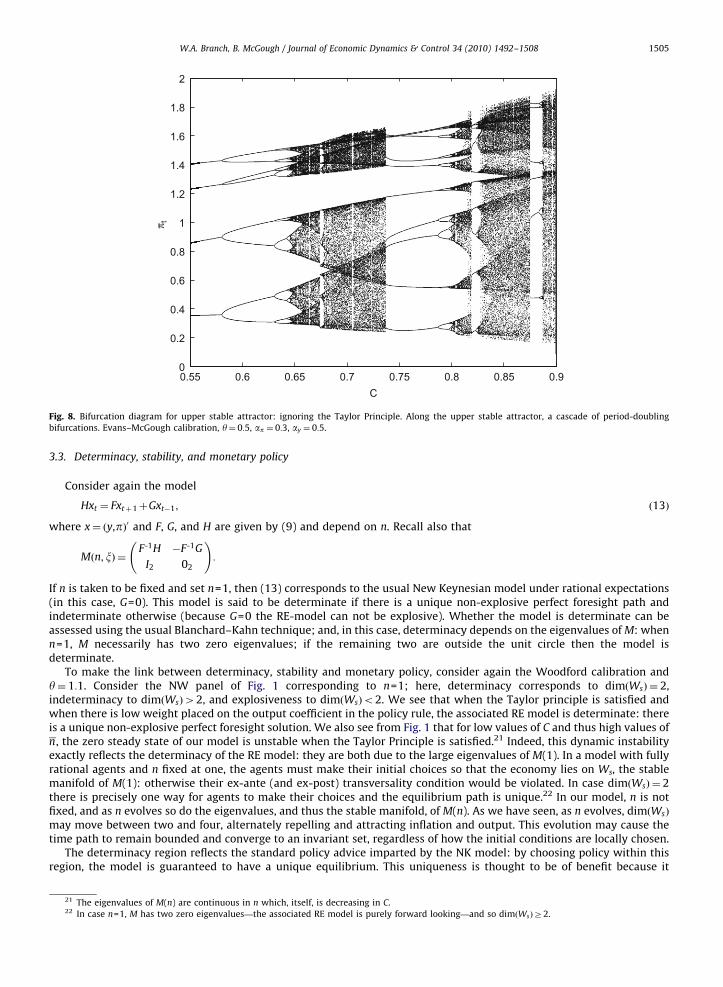
Qualitatively different behavior may arise under alternative calibrations, as is nicely illustrated in the bifurcationdiagram under the Evans–McGough calibration, which corresponds to a model with strong elasticities in the IS and ASrelations. Fig. 7 sets y¼ 0:5, ap ¼ 0:3 and ay ¼ 0:5. For small values of C the zero steady state is stable, as expected.However, Fig. 7 illustrates that as C increases the zero steady state destabilizes and a stable two cycle emerges.Interestingly, for C near #0.05 the system again bifurcates, but this time two distinct stable 2-cycles emerge, suggesting apitchfork bifurcation of the dynamic map’s second iterate. Here the ‘‘+’’ and ‘‘3’’ indicate dynamics resulting from differentinitial conditions.

Fig. 8 gives a more complete picture of the bifurcations under the alternative calibration and apo1. Fig. 8 plots thebifurcation diagram for the upper stable attractor, which was de-marked by ‘‘3’’ in Fig. 7. A similar picture (not shown)emerges for the lower attractor. Fig. 8 illustrates that as costs rise further a period doubling cascade emerges and results incomplex dynamics.

3.2.3. Discussion of resultsThe results in the above subsections indicate that complex dynamics can arise under various settings for

monetary policy and whether adaptive agents are extrapolative or dampening. It is useful to briefly review theseresults.

If adaptive agents are extrapolative, i.e. y41, then Fig. 1 demonstrates that increasing the steady-state fraction ofadaptive agents can enhance the stability of the steady state. With dynamic predictor selection, the economy switchesbetween stable and unstable dynamics, and this can occur regardless of whether policy satisfies the Taylor Principle. Withy41, altering the cost of the rational predictor can bifurcate the stable steady state and lead to stable attractors with someexhibiting complex dynamics.

On the other hand, if adaptive are dampening, i.e. yo1, then Fig. 2 shows that increasing the steady-state fraction ofadaptive agents can lead to instability of the steady state. It follows that the nature of the dynamics depends on themonetary policy coefficients. If yo1 and monetary policy satisfies the Taylor Principle, then there does not exist a stablesteady state with heterogeneous expectations. The dampening of adaptive expectations in this case is not sufficient tooffset the (unstable) forward dynamics arising from the perfect foresight agents. However, if monetary policy does notsatisfy the Taylor Principle, then depending on the cost to the rational predictor, then can exist multiple steady states andmultiple stable attractors. The results from this paper suggest that the interaction between the forward-looking behaviorof rational agents and the backward-looking behavior of adaptive agents can destabilize the economy, even whenmonetary policy is set to satisfy the Taylor principle.

ARTICLE IN PRESS

−0.2 −0.15 −0.1 −0.05 0 0.05 0.1 0.15 0.2−1

−0.8

−0.6

−0.4

−0.2

0

0.2

0.4

0.6

0.8

1

C

π t

Fig. 7. Stable 2-cycle bifurcates into two co-existing stable 2-cycles: ignoring the Taylor Principle. For #0:2oCo#0:005 there is a unique stabletwo-cycle, which for C4#0:005 bifurcates into two co-existing two cycles. Evans-McGough calibration, y¼ 0:5,ap ¼ 0:3,ay ¼ 0:5.


3.3. Determinacy, stability, and monetary policy

Consider again the model

Hxt ¼ Fxtþ1þGxt#1; ð13Þ

where x¼ ðy,pÞ0 and F, G, and H are given by (9) and depend on n. Recall also that

Mðn; xÞ ¼F-1H #F-1G

I2 02

!:

If n is taken to be fixed and set n=1, then (13) corresponds to the usual New Keynesian model under rational expectations(in this case, G=0). This model is said to be determinate if there is a unique non-explosive perfect foresight path andindeterminate otherwise (because G=0 the RE-model can not be explosive). Whether the model is determinate can beassessed using the usual Blanchard–Kahn technique; and, in this case, determinacy depends on the eigenvalues ofM: whenn=1, M necessarily has two zero eigenvalues; if the remaining two are outside the unit circle then the model isdeterminate.

To make the link between determinacy, stability and monetary policy, consider again the Woodford calibration andy¼ 1:1. Consider the NW panel of Fig. 1 corresponding to n=1; here, determinacy corresponds to dimðWsÞ ¼ 2,indeterminacy to dimðWsÞ42, and explosiveness to dimðWsÞo2. We see that when the Taylor principle is satisfied andwhen there is low weight placed on the output coefficient in the policy rule, the associated RE model is determinate: thereis a unique non-explosive perfect foresight solution. We also see from Fig. 1 that for low values of C and thus high values ofn, the zero steady state of our model is unstable when the Taylor Principle is satisfied.21 Indeed, this dynamic instabilityexactly reflects the determinacy of the RE model: they are both due to the large eigenvalues of M(1). In a model with fullyrational agents and n fixed at one, the agents must make their initial choices so that the economy lies on Ws, the stablemanifold of M(1): otherwise their ex-ante (and ex-post) transversality condition would be violated. In case dimðWsÞ ¼ 2there is precisely one way for agents to make their choices and the equilibrium path is unique.22 In our model, n is notfixed, and as n evolves so do the eigenvalues, and thus the stable manifold, of M(n). As we have seen, as n evolves, dimðWsÞmay move between two and four, alternately repelling and attracting inflation and output. This evolution may cause thetime path to remain bounded and converge to an invariant set, regardless of how the initial conditions are locally chosen.

The determinacy region reflects the standard policy advice imparted by the NK model: by choosing policy within thisregion, the model is guaranteed to have a unique equilibrium. This uniqueness is thought to be of benefit because it

ARTICLE IN PRESS

0.55 0.6 0.65 0.7 0.75 0.8 0.85 0.90

0.2

0.4

0.6

0.8

1

1.2

1.4

1.6

1.8

2

C

π t

Fig. 8. Bifurcation diagram for upper stable attractor: ignoring the Taylor Principle. Along the upper stable attractor, a cascade of period-doublingbifurcations. Evans–McGough calibration, y¼ 0:5, ap ¼ 0:3, ay ¼ 0:5.

21 The eigenvalues of M(n) are continuous in n which, itself, is decreasing in C.22 In case n=1, M has two zero eigenvalues—the associated RE model is purely forward looking—and so dimðWsÞZ2.


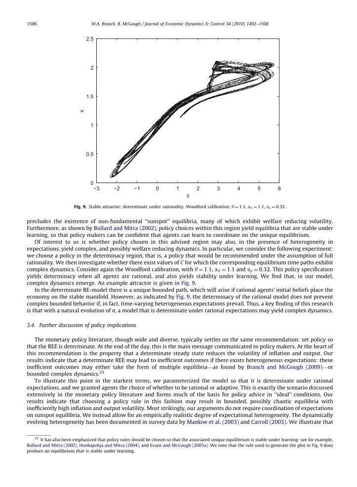
precludes the existence of non-fundamental ‘‘sunspot’’ equilibria, many of which exhibit welfare reducing volatility.Furthermore, as shown by Bullard and Mitra (2002), policy choices within this region yield equilibria that are stable underlearning, so that policy makers can be confident that agents can learn to coordinate on the unique equilibrium.

Of interest to us is whether policy chosen in this advised region may also, in the presence of heterogeneity inexpectations, yield complex, and possibly welfare reducing dynamics. In particular, we consider the following experiment:we choose a policy in the determinacy region, that is, a policy that would be recommended under the assumption of fullrationality. We then investigate whether there exist values of C for which the corresponding equilibrium time paths exhibitcomplex dynamics. Consider again the Woodford calibration, with y¼ 1:1, ap ¼ 1:1 and ay ¼ 0:32. This policy specificationyields determinacy when all agents are rational, and also yields stability under learning. We find that, in our model,complex dynamics emerge. An example attractor is given in Fig. 9.

In the determinate RE-model there is a unique bounded path, which will arise if rational agents’ initial beliefs place theeconomy on the stable manifold. However, as indicated by Fig. 9, the determinacy of the rational model does not preventcomplex bounded behavior if, in fact, time-varying heterogeneous expectations prevail. Thus, a key finding of this researchis that with a natural evolution of n, a model that is determinate under rational expectations may yield complex dynamics.

3.4. Further discussion of policy implications

The monetary policy literature, though wide and diverse, typically settles on the same recommendation: set policy sothat the REE is determinate. At the end of the day, this is the main message communicated to policy makers. At the heart ofthis recommendation is the property that a determinate steady state reduces the volatility of inflation and output. Ourresults indicate that a determinate REE may lead to inefficient outcomes if there exists heterogeneous expectations: theseinefficient outcomes may either take the form of multiple equilibria—as found by Branch and McGough (2009)—orbounded complex dynamics.23

To illustrate this point in the starkest terms, we parameterized the model so that it is determinate under rationalexpectations, and we granted agents the choice of whether to be rational or adaptive. This is exactly the scenario discussedextensively in the monetary policy literature and forms much of the basis for policy advice in ‘‘ideal’’ conditions. Ourresults indicate that choosing a policy rule in this fashion may result in bounded, possibly chaotic equilibria withinefficiently high inflation and output volatility. Most strikingly, our arguments do not require coordination of expectationson sunspot equilibria. We instead allow for an empirically realistic degree of expectational heterogeneity. The dynamicallyevolving heterogeneity has been documented in survey data by Mankiw et al. (2003) and Carroll (2003). We illustrate that

ARTICLE IN PRESS

−3 −2 −1 0 1 2 3 4 5 60

0.5

1

1.5

2

2.5

y

π

Fig. 9. Stable attractor: determinate under rationality. Woodford calibration, y¼ 1:1, ap ¼ 1:1, ay ¼ 0:32.

23 It has also been emphasized that policy rules should be chosen so that the associated unique equilibrium is stable under learning: see for example,Bullard and Mitra (2002), Honkapohja and Mitra (2004), and Evans and McGough (2005a). We note that the rule used to generate the plot in Fig. 9 doesproduce an equilibrium that is stable under learning.


if policy attempts to achieve a determinate REE in a New Keynesian model and these heterogeneous expectations dynamicsare present, the policy maker may unwittingly destabilize the economy. This suggests that policy should be designed toaccount for potentially destabilizing heterogeneity in a way that simple linear interest rate rules can not accomplish.

One may wonder how sensitive our results are to our specification of adaptive expectations, the predictor choicedynamic, and the model parameterization. We adopted an adaptive predictor with the same form as the MSV REE becauseit is the least ad hoc specification of adaptive expectations. We could instead specify adaptive beliefs in the Cagan sense as ageometric average of past observations. We believe that our qualitative results are robust to this specification because thekey for generating our findings is that adaptive and rational predictors return distinct forecasts out of steady state; thisproperty alters the stability properties of the steady state.

Similarly, the results are not sensitive to the predictor choice mechanism. In Branch and McGough (2005), weillustrated that a replicator dynamic will yield similar dynamic behavior, in a cobweb model, as the MNL of Brock andHommes (1997). Finally, we have endeavored to verify the existence of complicated dynamics across a broad spectrum ofcalibrations. The key is that for some for some n we have dimðWsðnÞÞ ¼ 4. Branch and McGough (2009) document anextensive region of the parameter space with this property. An open empirical question is whether the values of o and Care of reasonable magnitudes. Since o parameterizes the MSE, and C is measured in MSE units, there is no naturalinterpretation of these values in terms of utility or consumption units. An interesting extension would be to embed thepredictor choice into the agent’s recursive optimization problem.

4. Conclusion

This paper examines the impact of endogenous expectations heterogeneity on a model’s dynamic properties. Ourcentral finding is that an otherwise linear model may exhibit bounded complex dynamics if agents are allowed to selectbetween competing costly predictors (e.g. rational versus adaptive). These dynamics arise through the dual attracting andrepelling nature of the steady-state values of output and inflation—the nature of which depends on the proportions ofrational and adaptive agents. If the steady state is attracting for higher proportions of rational agents and repelling forlower proportions, then the natural tension between predictor cost and forecast accuracy mirrors the implied tension ofattracting and repelling dynamics. When the economy is far from the steady state, the accuracy benefits of the rationalpredictor outweighs its costs, and the proportion of rational agents rises, causing the steady state to become attracting andthereby drawing the economy toward it. As the economy approaches the steady state, the relative effectiveness of therational predictor falls, so that agents begin switching to the cheaper adaptive predictor. This switching causes the steadystate to repel the economy and the process repeats itself.

The complex dynamics produced by our model are not outcomes limited to unusual calibrations or a priori poor policychoices: complex behavior appears to be an almost ubiquitous feature of a time-varying heterogeneous expectations NewKeynesian model. Even policy designed to induce determinacy and stability under learning when levied against a rationalversion of the model may be insufficient to guard against the mentioned bad outcomes. We find that specifications ofpolicy rules satisfying the Taylor principle, and which yield determinacy under rationality, may result in bounded complexdynamics, and this possibility obtains even if all agents are initially rational.

References

Anufriev, M., Assenza, T., Hommes, C.H., Massaro, D., 2009. Interest rate rules and macroeconomic stability under heterogeneous expectations. CENDEFWorking Paper 08-08.

Benhabib, J., Eusepi, S., 2004. The design of monetary and fiscal policy: a global perspective. Journal of Economic Theory 123 (1), 40–73.Benhabib, J., Schmitt-Grohe, S., Uribe, M., 2001. The perils of Taylor rules. Journal of Economic Theory 96, 40–69.Bernanke, B., 2004. The great moderation, remarks by governor Ben S. Bernanke at the meetings of the Eastern Economic Association, Washington DC,

February 20, 2004.Bernanke, B., Woodford, M., 1997. Inflation forecasts and monetary policy. Journal of Money, Credit, and Banking 24, 653–684.Branch, W.A., 2002. Local convergence properties of a cobweb model with rationally heterogeneous expectations. Journal of Economic Dynamics and

Control 27 (1), 64–85.Branch, W.A., 2004. The theory of rationally heterogeneous expectations: evidence from survey data on inflation expectations. Economic Journal 114,

592–621.Branch, W.A., 2007. Sticky information and model uncertainty in survey data on inflation expectations. Journal of Economic Dynamics and Control 31 (1),

245–276.Branch, W.A., Evans, G.W., 2006. Intrinsic heterogeneity in expectation formation. Journal of Economic Theory 127, 264–295.Branch, W.A., McGough, B., 2005. Multiple equilibria in heterogeneous expectations models. Contributions to Macroeconomics, BE-Press, vol. 4, Issue 1,

Article 12.Branch, W.A., McGough, B., 2009. Monetary policy in a new Keynesian model with heterogeneous expectations. Journal of Economic Dynamics and

Control 33 (5), 1036–1051.Brazier, A., Harrison, R., King, M., Yates, T., 2008. The danger of inflating expectations of macroeconomic stability: heuristic switching in an overlapping

generations monetary model. International Journal of Central Banking 4 (2), 219–254.Brock, W.A., Dindo, P., Hommes, C.H., 2006. Adaptively rational equilibrium with forward looking agents. International Journal of Economic Theory 2

(3-4), 241–278.Brock, W., de Fountnouvelle, P., 2000. Expectational diversity in monetary economics. Journal of Economic Dynamics and Control 24, 725–759.Branch, W.A., Hommes, C.H., 1997. A rational route to randomness. Econometrica 65, 1059–1160.Brock, W.A., Hommes, C.H., 1998. Heterogeneous beliefs and routes to chaos in a simple asset pricing model. Journal of Economic Dynamics and Control

22, 1235–1274.

ARTICLE IN PRESSW.A. Branch, B. McGough / Journal of Economic Dynamics & Control 34 (2010) 1492–1508 1507

Bullard, J.M., Mitra, K., 2002. Learning about monetary policy rules. Journal of Monetary Economics 49, 1105–1129.Carroll, C.D., 2003. Macroeconomic expectations of households and professional forecasters. Quarterly Journal of Economics 118 (1), 269–298.Clarida, R., Gali, J., Gertler, M., 2000. Monetary policy rules and macroeconomic stability: evidence and some theory. Quarterly Journal of Economics 115,

147–180.DeGrauwe, P., 2008. Animal Spirits and Monetary Policy, CESifo Discussion Paper 2418.Evans, G.W., Honkapohja, S., 2005. Adaptive learning and monetary policy design. Journal of Money, Credit, and Banking 35, 1045–1072.Evans, G.W., Honkapohja, S., Mitra, K., 2003. Notes on Agents’ Behavioral Rules under Adaptive Learning and Recent Studies of Monetary Policy, mimeo.Evans, G.W., McGough, B., 2005a. Monetary policy, indeterminacy, and learning. Journal of Economic Dynamics and Control 29, 1809–1840.Evans, G.W., McGough, B., 2005b. Monetary policy, stable indeterminacy, and inertia. Economics Letters 87, 1–7.Gali, J., Lopez-Salido, J.D., Valles, J., 2004. Rule of thumb consumers and the design of interest rate rules. Journal of Money, Credit, and Banking 36 (4),

739–764.Guckenheimer, J., Holmes, P., 1983. Nonlinear Oscillations, Dynamical Systems, and Bifurcations of Vector Fields. Springer-Verlag, New York.Guse, E.A., 2008. Heterogeneous expectations, adaptive learning, and evolutionary dynamics, mimeo.Honkapohja, S., Mitra, K., 2004. Are non-fundamental equilibria learnable in models of monetary policy? Journal of Monetary Economics 51, 1743–1770Kuznetsov, Y., 1998. Elements of Applied Bifurcation Theory. Springer-Verlag, New York.Levin, A., Williams, J., 2003. Robust monetary policy with competing reference models. Journal of Monetary Economics 50, 945–975.Mankiw, N.G., Reis, R., Wolfers, J., 2003. Disagreement about inflation expectations. In: Gertler, M., Rogoff, K. (Eds.), NBER Macroeconomics Annual 2003.Manski, C.F., McFadden, D., 1981. Structural Analysis of Discrete Data with Econometric Applications. MIT Press, Cambridge, MA.Marcet, A., Nicolini, J-P., 2003. Recurrent hyperinflations. American Economic Review 93, 1476–1498.McCallum, B., Nelson, E., 1999. Performance of operational policy rules in an estimated semiclassical model. In: Taylor, J.B. (Ed.), Monetary Policy Rules.

University of Chicago Press, Chicago, pp. 55–119.Palis, J., Takens, F., 1993. Hyperbolicity and Sensitive Chaotic Dynamics at Homoclinic Bifurcations. Cambridge University Press.Pesaran, H.M., 1987. The Limits of Rational Expectations. Basil, Blackwell, Oxford.Preston, B., 2005a. Learning of monetary policy rules when long horizons matter. International Journal of Central Banking 1, 2.Preston, B., 2005b. Adaptive learning, forecast-based instrument rules and monetary policy. Journal of Monetary Economics 53 (3), 507–535.Svensson, L., Woodford, M., 2003. Implementing optimal policy through inflation-forecast targeting. In: Bernanke, B.S., Woodford, M. (Eds.), The Inflation

Targeting Debate. University of Chicago Press, Chicago.Taylor, J.B., 1999. Monetary Policy Rules. NBER Business Cycle Series, vol. 3.Tuinstra, J., Wagener, F.O.O., 2007. On learning equilibria. Economic Theory 30, 493–513.Woodford, M., 1999. Optimal monetary policy inertia. The Manchester School 67, 1–35 (Suppl.).Woodford, M., 2003. Interest and Prices. Princeton University Press.

ARTICLE IN PRESSW.A. Branch, B. McGough / Journal of Economic Dynamics & Control 34 (2010) 1492–15081508

dynamic predictor selection in a new ... - economics.uci.edu

Documents