dynamic properties of ice and frozen clay ...bibliographic data sheet 1 1. report no. msu-ce-76-4 4....
TRANSCRIPT

DYNAMIC PROPERTIES OF ICE AND FROZEN CLAY UNDERCYCLIC TRIAXIAL LOADING CONDITIONS
by
Ted S. Vinson and Thira ChaichanavongDepartment of Civil Engineering
Volume I of IIFinal Report of Research Conducted Under Research Grant ENG74-13506
SHEAR MODULI AND DAMPING FACTORS IN FROZEN SOILSfor the Period October 1, 1974 to September 30,1976
sponsored by theNATIONAL SCIENCE FOUNDATION
Washington, D.C. 20550
Report No. MSU-CE-76-4
October 1976
Division of Engineering ResearchMICHIGAN STATE UNIVERSITY
East Lansing, Michigan 48824


BIBLIOGRAPHIC DATASHEET 1
1. Report No.MSU-CE-76-4
4. Title and Subtitle
DYNAMIC PROPERTIES OF ICE AND FROZEN CLAY UNDERCYCLIC TRIAXIAL LOADING CONDITIONS
7. Aurhor(s)
Ted S. Vinson (Oregon State University)& Thira9. Performing Organization Name and Address
Division of Engineering ResearchMichigan State UniversityEast Lansing, Michigan 48824
12. Sponsoring Organization Name and Address
National Science FoundationWashington, D.C. 20550
5. ReporY I5at'e"" 'C'- ">'
October 19766.
8. Performing Organization Repr.Chaichanavong No.
10. Project/Task/Work Unit No.
11. Contract/Grant No.
ENG74-l3506
13. Type of Report & PeriodCovered Fina 1
pet. 1, 1974 to Sept. 30,'7614.
15. Supplementary Notes Volume I of II; Final Report of research conducted under projectentitled "Shear Moduli and Damping Factors 1n Frozen Soils"
16. Abstracts As part of a long-term study to evaluate dynamic properties of frozen soilsunder simulated earthquake and low frequency loading conditions, cyclic triaxial testswere performed on laboratory prepared samples of ice and frozen clay. The cylindricalpolycrystalline ice samples used in the research program were prepared using naturalsnow and distilled water. The samples were tested at strain amplitudes from 3 x 10- 3 tc2 x 10- 2%, temperatures from -1 to -10°C, frequencies from 0.05 to 5 cps and confiningpressures from 0 to 200 psi. The values of dynamic Young's modulus over the range ofmaterial and test conditions were from 260 x 103 to 900 x 103 psi; the values of dampingratio were from 0.001 to 0.14. Two types of frozen clay samples were used in theresearch program: (1) Ontonagon clay and (2) a mixture of Ontonagon and sodium montmorillonite clay (fifty percent each by weight). The samples were tested at strain amplitudes from 3 x 10- 3 to 1 x 10- 1%, temperatures from -1 to _10°C, frequencies from 0.05to 5 cps, and confining pressures from 0 to 200 psi. The values of dYDamic Young's modulus over the range of test conditions were from 90 x 103 to 880 x 103 psi; the values17. KeyWords and Document Analysis. 170. Desctiptors of damping ratio were from 0.02 to 0.30.* Geotechnical Engineering* Dynamics* Earthquakes* Permafrost* Ice* ClayCyclic "LoadingDampingYoung's ModulusTriaxial tests
IFrozen soils
17b~ Identifiers/Open-Ended Terms
,
III11?c. COSATI Field/Group 8/13; 8/12; 8/11 itYn . Availability Statement No restriction on distribution.
1··'~~~~~~'i~rl:;f"~.']~~~$:CQn
Ab"r::1l1-l.Ci;.<c,; y", ( lYCZ~('.". /f"!/7 /f,\
19.. Security Class (ThisReport)
UNC LA "IF IEf)20. Security Class (This
PageUNCLASSIFIED
-
22. Price if'/ ;,.-pC A/y/.~i·~·;
THrs FllH\l MAY BE RFPRr)[)r:(TD USCOMM·DC ~265·P74


FORI'JARD
This report presents the results from a research project entitled"Shear Moduli and Damping Factors in Frozen Soils" sponsored by the
National Science Foundation under Grant ENG74-13506. The PrincipalInvestigator for the research project was Dr. Ted S. Vinson, AssociateProfessor of Civil Engineering, Michigan State University. Mr. ThiraChaichanavong, Mr. Ronald L. Czajkowski, and Mr. John C. Li, GraduateResearch Assistants in the Division of Engineering Research, conductedthe laboratory tests associated with the study. Ms. Charlene Burns,Ms. Sheila Eddington, and Ms. Geraldine Wright, Undergraduate ResearchAides in the Division of Engineering Research, assisted in the datareduction and presentation. Mr. Dave Aditays and Mr. Elbert Mills,Undergraduate Research Aides in the Division of Engineering Research,assisted in the development and fabrication of the electronic instrumentation associated with the test system. Mr. Don Childs, Shop Supervisor in the Division of Engineering Research, assisted in the designand construction of the mechanical and hydraulic components associatedwith the test system. Ms. Charlene Burns typed the final draft of thereport. Finally, Dr. O.B. Andersland offered many helpful suggestionsduring the course of the study. His contribution is sincerely appreciated.
The results of the research project are presented in two volumesentitled: "Dynamic Properties of Ice and Frozen Clay Under CyclicTriaxial Loading Conditions" and "Dynamic Properties of Frozen Cohesionless Soils Under Cyclic Triaxial Loading Conditions. II The workpresented in this volume is associated with the development of thecyclic triaxial test system and experimental techniques employed toevaluate dynamic properties of ice and frozen clay, a discussion of theexperimental results, and a comparison of the experimental results ofthe present study to those of previous studies.
i.b


ABSTRACT
As part of a long-term study to evaluate dynamic properties of
frozen soils under simulated earthquake and low frequency loading conditions, cyclic triaxial tests were performed on laboratory preparedsamples of ice and frozen clay. The cyclic triaxial test setup consistsof four basic components: (1) an MTS electrohydraulic closed loop testsystem which applies a cyclic deviator stress to the sample, (2) a triaxial cell which contains the sample and noncirculating coolant, (3) arefrigeration unit and cold bath which circulates the coolant around thetriaxial cell, (4) output recording devices to monitor the load (stress)and displacement (strain) of the sample during the test.
The cylindrical polycrystalline ice samples used in the researchprogram were prepared using natural snow and aistilled water for highdensity samples (about 0.904 glee) or natural snow and carbonated waterfor low density samples (about 0.77 glee). The samples were tested atstrain amplitudes from 3 x 10⁻³ to 2 x 10⁻²%, temperatures from -1 to-10°C, frequencies from 0.05 to 5 cps and confining pressures from a to200 psi. The values of dynamic Young's modulus over the range of material and test conditions were from 260 x 103 to 900 x 103 psi; the values of damping ratio were from 0.001 to 0.14. The test results indicatethat the dynamic Young's modulus of ice increases, in general, withincreasing confining pressure, density, and frequency. The dynamicYoung's modulus of ice decreases with ascending temperature and increasing strain amplitude. The test results indicate that, in general, damping ratio of ice decreases as frequency increases from 0.05 to 1.0 cpsand increases as frequency increases from 1.0 to 5.0 cps. The dampingratio tends to decrease with descending temperature and increases withincreasing strain amplitude for high density ice. It is apparently notaffected by strain amplitude for low density ice. There appears to beno well-defined relationship between damping ratio of ice and confininqpressure or density.
Two types of frozen clay samples were used in the research program:(1) Ontonagon clay, termed "O-clay," and (2) a mixture of Ontonagon andsodium montmorillonite clay (fifty percent each by weight), termed "M +
O-clay." The O-clay was prepared at different water contents to assessthe influence of water (ice) content on dynamic properties. The M+ 0-
ii


clay was used to investigate the influence of specific surface area(related to unfrozen water content). The samples were tested at strain
-3 -1amplitudes from 3 x 10 to 1 x 10 %, temperatures from -1 to -10 0 e,frequencies from 0.05 to 5 cps, and confining pressures from 0 to 200
psi. The values of dynamic Young1s modulus over the range of test conditions were from 90 x 103 to 880 x 103 psi; the values of damping ratiowere from 0.02 to 0.3. The test results indicate that the dynamicYoung1s modulus of frozen clay decreases with increasing strain amplitudeand specific surface area: The dynamic Young1s modulus of frozen clayincreases with descending temperature and increasing water content andfrequency. It is apparently not affected by confining pressure. Thetest results indicate that the damping ratio of frozen clay increaseswith increasing strain amplitude and ascending temperature. The dampingratio, in general, decreases for an increase in frequency from 0.05 to5 cps; for frequencies greater than 5 cps, damping ratio increases asfrequency increases. There appears to be no well-defined relationshipbetween the damping ratio and water content or specific surface area.The damping ratio is apparently not affected by confining pressure.
The dynamic properties of ice and frozen clay obtained in the present study at the lowest strain amplitude were compared to those obtainedin previous studies. The values of longitudinal and compressional wavevelocities of ice determined in the present study are lower than comparable wave velocities determined in previous laboratory &field studies.This may be a consequence of the fact that the strain amplitude of te~t
ing in the present study is greater than those associated with previousstudies and the test frequencies in the present study are much lower thanthose associated with previous studies. The values of damping ratio ofice determined in the present are close to the values obtained in previous studies. The values of longitudinal wave velocities of frozenclay obtained in the present study compare favorably with the resultsfrom previous studies. It appears any differences in longitudinal wavevelocities can be explained by differences in the test techniques andmaterial types employed between the present and previous studies. Thevalues of damping ratio of frozen clay obtained in the present study areclose to values obtained in one previous laboratory study.
iii


TABLE OF CONTENTS
FORWARD .ABSTRACT .LIST OF TABLES.LIST OF FIGURESLIST OF SYMBOLS
Chapter
Page
ii i
viiviiixvii
1.
2.
3.
INTRODUCTION .1.1. Statement of the Problem .1.2. Purpose and Scope of Studies.1.3. Background. . . . . . . . .. ... ..
1.3.1. Mechanical Properties of Frozen Soils,Thermal Characteristics of Frozen SoilDeposits and Dynamic Properties ofUnfrozen Soils .
1.3.2. Fundamentals of Cyclic Triaxial Testing
DYNAMIC PROPERTIES OF ICE AND FROZEN CLAY .2 . 1 . Ge ne ra1 . . . . . . . . . . . , . . .2.2. Previous Methods to Evaluate Dynamic
Properties of Ice and Frozen Clay2.3. Dynamic Elastic Properties of Ice
2.3.1. Effect of Temperature .2.3.2. Effect of Density .2.3.3. Effect of Frequency .2.3.4. Effect of Confining Pressure.
2.4. Damping of Ice .2.5. Dynamic Elastic Properties of Frozen Clay
2.5.1. Effect of Void Ratio .2.5.2. Effect of Ice Saturation .2.5.3. Effect of Temperature .2.5.4. Effect of Frequency .2.5.5. Effect of Unfrozen Water Content.2.5.6. Effect of Dynamic Stress (or
Strain) . . . . . . . . .2.6. Damping of Frozen Clay .2.7. Poisson1s Ratio of Ice and Frozen Clay.
2.7.1. Poisson's Ratio of Ice.....2.7.2. Poisson1s Ratio of Frozen Clay.
SAMPLE PREPARATION, SAMPLE INSTALLATION,TRIAXIAL CELL ASSEMBLY, AND TEST PROCEDURE.3.1. General .3.2. Preparation of Ice Sample .3.3. Preparation of Frozen Clay Sample ..3.4. Sample Installation and Triaxial Cell
Assembly .3.5. Test Procedure .
iv
1
123
34
7
7
7171721232626292929293232
3636363838
43
434345
5052


Chapter Page
4. DYNAMIC PROPERTIES OF ICE UNDER CYCLIC TRIAXIAL LOADING CON-DITIONS . . . . . . . . . . . . . . . 55
4.1. General........ . . . . 554.2. Test History Effects on Dynamic
Properties. . . . . . . . . . . 554.3. Influence of Number of Cycles on
Evaluation of Dynamic Properties. 594.4. Dynami c Young 's Modul us of Ice. . . 59
4.4.1. Effect of Strain Amplitude. . 634.4.2. Effect of Confining Pressure. 644.4.3. Effect of Frequency. . . . 764.4.4. Effect of Temperature. . . 794.4.5 Effect of Density. . . . . 82
4.5. Damping Ratio of Ice. . . . . . . . 824.5.1. Effect of Strain Amplitude. 854.5.2. Effect of Frequency. . . . 854.5.3. Effect of Temperature. . . 904.5.4. Effect of Density . . . . . . 914.5.5. Effect of Confining Pressure. 91
5. DYNAMIC PROPERTIES OF FROZEN CLAY UNDER CYCLIC TRIAXIALLOADING CONDITIONS. 93
5.1. General... . . . . . . . . . . 935.2. Test History. . . . . . . . . . . 935.3. Influence of Number of Cycles on
Evaluation of Dynamic Properties. 955.4. Dynamic Young's Modulus of Frozen Clay. 100
5.4.1. Effect of Strain Ampl itude. . 1005.4.2. Effect of Frequency. . . . . . 1075.4.3. Effect of Temperature. . . . . 1095.4.4. Effect of Water Content. . . . . 1095.4.5. Effect of Specific Surface Area 114
5.5. Damping Ratio of Frozen Clay. . . . 1145.5.1. Effect of Strain Ampl itude. . 1145.5.2. Effect of Frequency. . . . . . 1175.5.3. Effect of Temperature. . . . . 1245.5.4. Effect of Water Content. . . . . 1245.5.5. Effect of Specific Surface Area 129
6. COMPARISONS OF DYNAMIC PROPERTIES OF ICE ANDFROZEN CLAY . . . . . . . . . . . . . . . 1316. 1. General . . . . . . . . . . . . . . . . 1316.2. Comparison of Dynamic Properties of Ice 132
6.2.1. Longitudinal and Compression WaveVelocity. . . . . . . . . . . . . 132
6.2.2. Damping Ratio. . . . . . . . . . 1346.3. Comparison of Dynamic Properties of Frozen
Cl ay. . . . . . . . . . . . . . . . . . . 1376.3.1. Longitudinal and Compression Wave
Velocity. . . 1376.3.2. Damping Ratio.. 140
v


Chapter
7. SUMMARY AND CONCLUSIONS
LIST OF REFERENCES.
APPENDIX
Page
143
151
A. DESCRIPTION OF CYCLIC TRIAXIAL TEST EQUIPMENT 156A.l. The MTS E1ectrohydrau1ic Closed Loop
Test System . · · · · · · · · · 156A.l.l. MTS 406.11 Controller 160A.1.2. MTS 436.11 Controller 165
A.2. Triaxial Cell · · · · · · · · 167A.3. Cooling System. · · · · · · · 172A.4. Output Recording System . · · 175
B. DESCRIPTION OF SAMPLE COUPLING DEVICE 181
C. CYCLIC TRIAXIAL TEST RESULTS - DYNAMIC YOUNG1SMODULUS OF ICE. . · · · · · · · · · · · · . · . · · 185
D. CYCLIC TRIAXIAL TEST RESULTS - DAMPING RATIOOF ICE. . . . · · · · · · · · · · . · · . . · . 223
E. CYCLIC TRIAXIAL TEST RESULTS - DYNAMIC YOUNG'SMODULUS OF FROZEN CLAY. · · · · · · · · · . · · · · . · . 239
F. CYCLIC TRIAXIAL TEST RESULTS - DAMPING RATIOOF FROZEN CLAY. . . · · · · · · · · · · · . · · . . · 264
vi

Table
2. 1
3.1
3.2
4.1
4.2
5.1
5.2
LIST OF TABLES
Conversion Equations Between Terms to CharacterizeDynamic Properties .Index and Mineralogical Properties of O-Clay and M+ 0-Clay .Water Content and Density of Clay Samples .Variation of Dynamic Young's Modulus of High Density Icewith Number of Cycles .Variation of Damping Ratio of High Density Ice with Num-ber of Cycles .Variation of Dynamic Young's Modulus of Frozen Clay withNumber of Cycles .Variation of Damping Ratio of Frozen Clay with Number ofCycl es. . . . . . . . . . . . . . . . . . . . . . . . . .
vii
Page
8
46
49
60
61
96
97


Figure
LIST OF FIGURES
Page
1.1 Stress State in Triaxial Tests with Cyclic Axial Stress 51.2 Deviator Stress Versus Axial Strain for One Load Cycle. 52.1 Electromagnetic Three-Mode Beam Vibrator (after Kaplar,
1969) . . . . . . . . . . . . . . . . . . . . . . . . . 102.2 Schematic of Forced Vibration Dynamic Test Equipment (after
Smi th, 1969). . . . . . . . . . . . . . . 112.3 Ultrasonic Pulsing Method (after Bennett, 1972) . . . . .. 132.4 Critical Angle Method , 142.5 Schematic of Forced Vibration Dynamic Test Equipment (after
Stevens, 1973) , 162.6 P-Wave Velocity of Ice Versus Temperature (after Roethlis-
berger, 1972) , 182.7 S-Wave Velocity of Ice Versus Temperature (after Roethlis-
berger, 1972) . . . . . . . . . . . . . . . . . . . . . 192.8 P-Wave Velocity in the Principal Directions of Single
Crystal Ice Versus Temperature (after Brockamp andQuerfurth from Roethlisberger, 1972). . . . . . . . . . 19
2.9 Sound Velocity in Synthetic Ice Cores Versus Temperature(after MUll er, 1961, from Roeth1i sberger, 1972). . . . .. 20
2.10 Summary of Longitudinal or P-Wave Velocities in IceMeasured by Various Investigators (after Kaplar, 1969). 20
2.11 P-Wave Velocity of Ice Versus Density (after Roethlisberger,1972) " 22
2.12 P-Wave Velocity Versus Ice Density From Seismic and Ultra-soni c Measurements (after Bennett, 1972). . .. .... 24
2.13 S-Wave Velocity Versus Ice Density From Seismic and Ultra-sonic Measurements (after Bennett, 1972). . . . .. 24
2.14 P-Wave Velocity of Ice Versus Depth at Camp Century (afterClarke, 1966) " 25
2.15 Complex Dynamic Moduli of Ice Versus Frequency (after Smith,1969) . . . . . . . . .. 25
2.16 Loss Factor of Ice Versus Frequency (after Smith, 1969) .. 272.17 Loss Factor of Ice Versus Drivinq Force (after Smith, 1969) 272.18 Loss Factor of Ice Versus Density (after Smith, 1969) .. , 282.19 Effect of Temperature on Tan 8 of Ice (after Stevens, 1975) 282.20 Sound Velocity in Synthetic Frozen Cores at Two Porosities
Versus Temperature (after MUller, 1961, from Roethlisberger,1972) . . . . . . . . . . . . . . . . . . . . . . .. 30
viii


Figure
2.21
2.22
2.23
2.24
2.25
2.26
2.27
2.28
2.292.30
3. 1
3.23.3
3.4
4.14.2
4.3
4.4
4.5
4.6
4.7
4.8
4.9
Effect of Ice Saturation on Complex Shear Modulus forFrozen Suffield Clay (after Stevens, 1973) .S-Wave Velocity Versus Temperature for Frozen Goodrich Clay(after Nakano and Froula, 1973) .Longitudinal Wave Velocity Versus Temperature for FrozenBoston Blue Clay and Fargo Clay (after Kaplar, 1969) ...
Effect of Temperature on Complex Moduli of Frozen GoodrichClay (modified after Stevens, 1975) .Dilational Velocity and Unfrozen Water Content Versus Temperature (after Nakano and Froula, 1973) .....Effect of Temperature on Tan 8 of Frozen Goodrich Clay(modified after Stevens, 1975) .Poisson's Ratio of Ice Versus Temperature (after Kaplar,1969) . . . . . . . . . . . . . . . . . . . . . . .Poisson's Ratio for Dry Snow Versus Density (after Mellorfrom Roethlisberger, 1972) .Poisson's Ratio of Ice Versus Density (after Smith, 1969)Poisson's Ratio of Frozen Clay Versus Temperature (afterKaplar, 1969) .Hollow Cylindrical Teflon Mold and Sample Caps with Coup-1i ngs '.' . . . . . . . . .Typical Cylindrical Ice Sample .Typical Cylindrical Frozen Clay Sample .Observed Hysteresis Loop for LVDT Core in Contact withHousing . . . . . . . . . . . . . . . . . . .Diagram of Acceptable Test History for Ice .Typical Records Obtained During Cyclic Triaxial Testing ofIce . . . . . . . . . . . . . . . . . . . . . . . . . .Least Squares Best Fit Line for Dynamic Young's Modulus ofHigh Density Ice Versus Axial Strain .Least Squares Best Fit Line for Dynamic Young's Modulus ofLow Density Ice Versus Axial Strain. . . ...Dynamic Young's Modulus Versus Axial Strain for High Density Ice at -1°C and 0.05 cps. . . . . .. . ....Dynamic Young's Modulus Versus Axial Strain for High Den-sity Ice at -1°C and 0.3 cps '. . .Dynamic Young's Modulus Versus Axial Strain for High Density Ice at -1°C and 1.0 cps. . . . . . .. . ....Dynamic Young's Modulus Versus Axial Strain for High Density Ice at -1°C and 5.0 cps. . . . . . .. . ....Dynamic Young's Modulus Versus Axial Strain for High Den-sity Ice at -2°C and 0.05 cps. . . . . .. . .....
ix
Paqe
31
31
33
33
35
37
39
4040
41
444448
5157
62
65
65
66
66
66
66
67


Figure
4.10
4.11
4.12
4.13
4.14
4. 15
~. 16
4.17
4.18
4.19
4.20
4.21
4.22
4.23
4.24
4.25
4.26
4.27
4.28
4.29
4.30
Dynamic Young's Modulus Versus Axial Strain for High Den-sity Ice at -2°e and 0.3 cps.. .Dynamic Young's Modulus Versus Axial Strain for High Density Ice at -2°e and 1.0 cps.Dynamic Young's Modulus Versus Axial Strain for High Den-sity Ice at -2°C and 5.0 cps. . . ..Dynamic Young's Modulus Versus Axial Strain for High Den-sity Ice at -4°C and 0.05 cps .. .Dynamic Young's Modulus Versus Axial Strain for High Den-sity Ice at -4°e and 0.3 cps.. .Dynamic Young's Modulus Versus Axial Strain for High Den-sity Ice at -4°C and 1.0 cps. . . .Dynamic Young's Modulus Versus Axial Strain for High Den-sity Ice at -4°e and 5.0 cps .. , ... . ..Dynamic Young's Modulus Versus Axial Strain for High Density Ice at -6°C and 0.3 cps. . . . . . . .. .Dynamic Young's Modulus Versus Axial Strain for High Density Ice at -6°e and 1.0 cps. . .. ... . ..Dynamic Young's Modulus Versus Axial Strain for High Density Ice at -6°e and 5.0 cps. .. .... ..Dynamic Young's Modulus Versus Axial Strain for High Den-sity Ice at -lOoe and 0.05 cps. .... . .Dynamic Young's Modulus Versus Axial Strain for High Density Ice at -lOoe and 0.3 cps. ... ..Dynamic Young's Modulus Versus Axial Strain for High Density Ice at -lOoe and 1.0 cps. .... . ...Dynamic Young's Modulus Versus Axial Strain for High Den-sity Ice at -lOoe and 5.0 cps. . ....Dynamic Young's Modulus Versus Axial Strain for Low DensityIce at -loe and 0.3 cps. . . . . . . . . . . ...Dynamic Young's Modulus Versus Axial Strain for Low DensityIce at -loe and 1.0 cps. .. ..... .Dynamic Young's Modulus Versus Axial Strain for Low DensityIce at -lee and 5.0 cps. ... .. . ..Dynamic Young's Modulus Versus Axial Strain for Low DensityIce at -4°e and 0.3 cps .... " " ...Dynamic Young's Modulus Versus Axial Strain for Low DensityIce at _4°C and 1.0 cps.. . . ... . ...Dynamic Young's Modulus Versus Axial Strain for Low DensityIce at -4°e and 5.0 cps. . .. . ... . ..Dynamic Young's Modulus Versus Axial Strain for Low DensityIce at -woe and 0.3 cps. .... ..
x
Page
67
67
67
68
68
68
68
69
69
69
70
70
70
70
71
71
71
72
72
72
73


Figure
4.31
4.32
4.33
4.34
4.35
4.36
4.37
4.38
4.39
4.40
4.41
4.42
Dynamic Young's Modulus Versus Axial Strain for Low DensityIce at -10°C and 1.0 cps. .. .. .Dynamic Young's Modulus Versus Axial Strain for Low DensityIce at -10°C and 5.0 cps. . . .. . ..Dynamic Young's Modulus Versus Confining Pressure for HighDensity Ice at -1°C. .Dynamic Young's Modulus Versus Confining Pressure for HighDensity Ice at -2°C . . . . . .. .. .Dynamic Young's Modulus Versus Confining Pressure for HighDensity Ice at -4°C. .. '" ...Dynamic Young's Modulus Versus Confining Pressure for HighDensity Ice at _6°C . . . . .. .. .... .Dynamic Young's Modulus Versus Confining Pressure for HighDensity Ice at -10°C.. '" . .. ..Dynamic Young's Modulus Versus Confining Pressure for LowDensity Ice at -1°C ..Dynamic Young's Modulus Versus Confining Pressure for Low'Dens ity Ice at -4°C . . . . . . " .Dynamic Young's Modulus Versus Confining Pressure for LowDensity Ice at -10°C. . . . . . .. .... .Dynamic Young's Modulus Versus Frequency for High DensityIce at -1°C. . .. . . . .. .Dynamic Young's Modulus Versus Frequency for High DensityIce at -2°C . . . . . . . .. .. .. ...
Page
73
73
74
74
74
74
75
75
75
75
77
77
4.43
4.44
Dynamic Young'sIce at -4°C ..Dynamic Young'sIce at -6°C . .
Modulus Versus Frequency for High Density
Modulus Versus Frequency for High Density77
77
4.45 Dynamic Young's Modulus Versus Frequency for High DensityIce at -10°C. . . . . . . . . . . . . . ... .. 78
4.46 Dynamic Young's Modulus Versus Frequency for Low DensityIce at -1°C. . . . . . . . . . . . . . . . . . . . . .. 78
4.47
4.48
Dynamic Young'sIce at -4°C . .Dynamic Young'sIce at -10°C..
Modulus Versus Frequency for Low Density
Modulus Versus Frequency for Low Density78
784.49
4.50
4.51
Dynamic Young's Modulus Versus Temperature for HighIce at a Confining Pressure of 25 psi ... .,Dynamic Young's Modulus Versus Temperature for HighIce at a Confining Pressure of 50 psi . . . .Dynamic Young's Modulus Versus Temperature for HighIce at a Confining Pressure of 100 psi. . ....
xi
Density
Densi.ty
Density
80
80
80


Figure Page
4.52 Dynamic Young's Modulus Versus Temperature for High DensityIce at a Confining Pressure of 200 psi. .. .... . 80
4.53 Dynamic Young's Modulus Versus Temperature for Low DensityIce at a Confining Pressure of 0 psi. .. ... .... 81
4.54 Dynamic Young's Modulus Versus Temperature for Low DensityIce at a Confining Pressure of 25 psi . . . . . . .. .. 81
4.55 Dynamic Young's Modulus Versus Temperature for Low DensityIce at a Confining Pressure of 50 psi . . . .. .... 81
4.56 Dynamic Young's Modulus Versus Temperature for Low DensityIce at a Confining Pressure of 100 psi.. .. 81
4.57 Dynamic Young's Modulus Versus Density of Ice at -1°C forThree Frequencies. . 83
4.58 Dynamic Young's Modulus Versus Density of Ice at -4°C forThree Frequencies . . . . . . . .. .. ... 83
4.59 Dynamic Young's Modulus Versus Density of Ice at -10°C forThree Frequencies . . . . . . . . . . .. ... 83
4.60 Dynamic Young's Modulus Versus Density of Ice at -1°C forThree Confining Pressures . . . . . . . . . . 84
4.61 Dynamic Young's Modulus Versus Density of Ice at -4°C forFour Confining Pressures. . . . . . . .. .... 84
4.62 Dynamic Young's Modulus Versus Density of Ice at -10°C forFour Confining Pressures. . . . . . . . . . . . 84
4.63 Least Squares Best Fit Line for Damping Ratio of High Den-sity Ice Versus Axial Strain. . . .... 86
4.64 Least Squares Best Fit Line for Damping Ratio of Low Den-sity Ice Versus Axial Strain. . . . . . .... 86
4.65 Damping Ratio Versus Axial Strain for High Density Ice at0.05 cps. 87
4.66 Damping Ratio Versus Axial Strain for High Density Ice at0.3 cps . .. . . .. 87
4.67 Damping Ratio Versus Axial Strain for High Density Ice at1.0 cps . . . .. 87
4.68 Damping Ratio Versus Axial Strain for High Density Ice at5.0 cps ... . . . . . . . . . . 87
4.69 Damping Ratio Versus Axial Strain for Low Density Ice at0.3 cps ... . .. .. .. 88
4.70 Damping Ratio Versus Axial Strain for Low Density Ice at1.a cps . . . . . . . . . ... 88
4.71 Damping Ratio Versus Axial Strain for Low Density Ice at5.0 cps .... ... 88
4.72 Damping Ratio Versus Frequency for High Density Ice. 89
xii


Figure
4.73 Damping Ratio Versus Frequency for Low Density Ice. 89
4.74 Damping Ratio Versus Temperature for High Density Ice 89
4.75 Damping Ratio Versus Temperature for Low Density Ice. 89
4.76 Damping Ratio Versus Frequency for Ice at Two Densities. 92
4.77 Damping Ratio Versus Temperature for Ice at Two Densities 92
4.78 Typical Variation of Damping Ratio with Confining Pressure. 92
5.1 Diagram of Acceptable Test History for Frozen Clay. . 945.2 Typical Record of Load and Displacement Obtained During
Cyclic Triaxial Testing of Frozen Clay. . . . . . . 98
5.3 Typical Hysteresis Loops (non-dimensional) Obtained DuringCyclic Triaxial Testing of Frozen Clay. . . . . . 99
5.4 Dynamic Young's Modulus Versus Confi~ing Pressure for 0-Clay at an Axial Strain of 1.1 x 10- %. . . . . . . . .. 101
5.5 Dynamic Young's Modulus Versus Axial Strain for O-Clay at0.3 cps and 29.2% Water Content .. ... ... 102
5.6 Dynamic Young's Modulus Versus Axial Strain for O-Clay at1.0 cps and 29.2% Water Content.. . 102
5.7 Dynamic Young's Modulus Versus Axial Strain for O-Clay at5.0 cps and 29.2% Water Content . .. ..... 102
5.8 Dynamic Young's Modulus Versus Axial Strain for O-Clay at0.05 cps and 36.0% Hater Content. ... .... 103
5.9 Dynamic Young1s Modulus Versus Axial Strain for O-Clay at0.3 cps and 36.0% Water Content.. .. .. . .. 103
5.10 Dynamic Young's Modulus Versus Axial Strain for O-Clay at1.0 cps and 36.0% Water Content. . . . .. 103
5.11 Dynamic Young1s Modulus Versus Axial Strain for O-Clay at5.0 cps and 36~0% Water Content . . 103
5.12 Dynamic Young's Modulus Versus Axial Strain for O-Clay at0.3 cps and 46.3% Water Content. . . . .. . .... 104
5.13 Dynamic Young's Modulus Versus Axial Strain for O-Clay at1.0 cps and 46.3% Water Content ..... .. . 104
5.14 Dynamic Young's Modulus Versus Axial Strain for O-Clay at5.0 cps and 46.3% Water Content. . . . . .. ... 104
5.15 Dynamic Young's Modulus Versus Axial Strain for O-Clay at0.3 cps and 55.1% Water Content. . . . .. .... 105
5.16 Dynamic Young's Modulus Versus Axial Strain for O-Clay at1.0 cps and 55.1% Water Content. . . . . . .. 105
5.17 Dynamic Young's Modulus Versus Axial Strain for O-Clay at5.0 cps and 55.1% Water Content. . . . . 105
5.18 Dynamic Young's Modulus Versus Axial Strain for M+ 0-Clay at 0.3 cps and 57.2% Water Content . 106
xiii


Figure
5.19
5.20
5.21
5.22
5.23
5.24
5.25
5.26
5.27
5.28
5.29
5.30
5.31
5.32
5.33
5.34
5.35
5.36
5.37
5.38
5.39
xiv
· · · · · · ·for a-Clay at -4°C and· · · · · · ·for a-Clay at -lOoC and· · · · · · · . · · · ·for O-Clay at -1°C and· · · · · . · · · · .for a-Clay at -4°C and· · · · · · · · · ·
Page


Figure
5.40
5.41
Damping Ratio Versus Axial Strain36.0% Water Content. .. ..Damping Ratio Versus Axial Strain46. 3% l~ater Content. .....
for a-Clay at -10°C and
for a-Clay at -1°C and
Page
119
1205.42 Damping Ratio Versus Axial Strain for a-Clay at -4°C and
46.3% Water Content 1205.43 Damping Ratio Versus Axial Strain for a-Clay at -10°C and
46.3% Water Content. . . 1205.44
5.45
5.46
5.47
5.48
5.49
Damping Ratio Versus Axial Strain55.1% Water Content .Damping Ratio Versus Axial Strain55.1% Water Content. .....Damping Ratio Versus Axial Strain55.1% Water Content .Damping Ratio Versus Axial Strainand 57.2% Water Content .. ..Damping Ratio Versus Axial Strainand 57.2% Water Content . .. .Damping Ratio Versus Axial Strainand 57.2% Water Content. ..,
for a-Clay at -1°C and
for a-Clay at -4°C and
for a-Clay at -10°C and
for M+ a-Clay at -1°C
for M+ a-Clay at -4°C
for M+ a-Clay at -10°C
121
121
121
122
122
1225.50
5.51
5.52
5.53
5.54
5.55
5.56
5.57
5.58
5.59
5.60
Damping Ratio Versus Frequency for a-Clay at an AxialStrain of 3.16 x 10⁻³%. . . . . . . . . . . . . 123Damping Rat10 Versus Frequency for a-Clay at an AxialStrain of 1.0 x 10⁻¹% . . . . . . . . . . . . . 123Damping Ratio Versus Frequency for a-Clay Tested to 50.0cps.. . . 123Damping Ratio Versus
3Temperature for a-Clay at an Axial
Strain of 3.16 x 10- %. . . . . . . . . . . . . . . . .. 125Damping Ratio Versus Temperature for a-Clay at an AxialStrain of 1.0 x 10⁻¹% . . . . . . . . . . . . . . . . . 125Damping Ratio Versus Water Content for a-Clay at -1°C andan Axial Strain of 3.16 x 10- 3% " 126Damping Ratio Versus Water Content for a-Clay at -1°C andan Axial Strain of 1.0 x 10⁻¹%. . . . . . . . . . . . 126Damping Ratio Versus Water Co~tent for a-Clay at -4°C andan Axial Strain of 3.16 x 10- % . . . . . . . . . . . 127Damping Ratio Versus Water C?ntent for a-Clay at -4°C andan Axial Strain of 1.0 x 10- %. . . . . . . . . . . . 127Damping Ratio Versus Water Co~tent for a-Clay at -10°C andan Axial Strain of 3.16 x 10- % 128Damping Ratio Versus Water C9ntent for a-Clay at -lOoe andan Axial Strain of 1.0 x 10- % 128
xv


Figure Page
5.61 Damping Ratio Versus Temperature for a-Clay and M+ a-Clayat an Axial Strain of 3.16 x 10⁻³%. . . . . . . . . . . . . 130
5.62 Damping Ratio Versus Temperature for a-Clay and M+ a-Clayat an Axial Strain of 1.0 x 10⁻¹% . . . . . . . . . . .. 130
6.1 Wave Velocity Versus Temperature of Ice 1336.2 Wave Velocity Versus Density of Ice. . . . . . 1356.3 Damping Ratio Versus Temperature of Ice. . . . 1366.4 Wave Velocity Versus Temperature of Frozen Clay 1386.5 Damping Ratio Versus Temperature of Frozen Clay 141
xvi


AL
AT
B
cp
0
Ed
EfELE*
F, f
G
G*
S
T
tan 8/2
VLVlq
Vp' P-wave
VS' S-wave
Wu
ex;
8
t.A
t.L
e
ed
LIST OF SYMBOLS
area of hysteresis loop
area of triangle
pore pressure parameter
confining pressure
damping ratio
dynamic Young's modulus
Young's modulus (flexural vibration)
Young's modulus (longitudinal vibration)
complex Young's modulus
frequency
(dynamic) shear modulus or dynamic modulus of rigidity
complex shear modulus
specific surface area
temperature
loss factor
longitudinal wave velocity
velocity of incident wave in bath liquid
compression wave velocity
shear wave velocity
unfrozen water content
angle of incidence between wave train and sample face
lag angle between stress vector and strain vector
axial strain
lateral strain
temperature
angle of refraction for longitudinal wave
xvii


8S
A-
].1
].1*
P
I
O"m
0"1 ' 0"2' 0"3
angle of refraction for shear wave
damping ratio
Poisson's ratio
complex Poisson's ratio
density
mean principal effective stress
major, intermediate, and minor principal stress
xviii


CHAPTER 1
INTRODUCTION
1.1 Statement of the ProblemIn the past decade considerable attention has been focused on
Alaska owing to its abundance of natural resources, particularly thoserelated to our increasing demand for energy. The Alaskan pipeline,presently under construction, represents a monumental engineeringundertaking to recover an estimated 25 to 30 billion barrels of petroleum beneath Alaska1s North Slope; plans have recently been announcedby El Paso Natural Gas Company to develop and bring into productionthe gas fields beneath Prudhoe Bay, which contain an estimated 25trillion cubic feet of natural gas; undoubtedly, many other projectswi 11 fo 11 ow.
With the recovery of natural resources, significant developmentof transporting facilities, transportation systems, utility networks,and general civil and industrial works must occur. Engineers concerned with this development will be faced with many challenging problems associated with the fact that 85 percent of Alaska lies withina permafrost region, i.e., a region of perenially or permanentlyfrozen ground (Brown and Pewe, 1973). Clearly, knowledge of thebehavior of frozen soils is essential to the solution of permafrostrelated problems.
Further, Alaska is located in one of the world1s most activeseismic zones. This was exemplified by the 1964 "Good Friday" earthquake and more than sixty other earthquakes that have equaled orexceeded a Richter magnitude of 7 since the 1800 l s (Davis and Echols,1962) .
It is now generally accepted that the ground surface motions whichoccur during an earthquake are influenced to a large extent by the characteristics of the underlying soil deposit under dynamic loading conditions (Idriss and Seed, 1968; Seed and Idriss, 1969). The importanceof soil conditions and ground motions to the response of structures hasbeen recognized for over half a century (Wood, 1908) and demonstratedconclusively in several recent earthquakes (Seed and Idriss, 1971; Seed,et al, 1972). Several analytic techniques are presently available topredict ground surface motions during earthquakes (Idriss and Seed, 1968;
1

2
Lysmer, et al, 1974; Schnabel, Lysmer, and Seed, 1972; Streeter, Wylie,and Richart, 1974). To employ these techniques two soil properties arerequired: (1) the dynamic shear modulus, and (2) the damping ratio.(These properties are also required to determine the response of foundations subjected to vibratory loads.) For unfrozen soils these properties have been determined by several investigators, usinq field and laboratory techniques, and design equations and curves to establish theproperties for representative soil types have been developed (Hardin andDrnevich, 1972; Seed and Idriss, 1970). For frozen soils these properties (or equivalent properties) have been evaluated from seismic fieldstudies and from ultrasonic, forced vibration, and resonant column testsin the laboratory. In general, however, it appears that the majority ofthese studies may be associated with test ranges that would not be usefulin earthquake response analyses. Thus, an engineer confronted with aseismic design problem involving frozen soils cannot use existing analytic techniques to predict ground surface motions because the necessaryproperties of frozen soils have not been determined.
1.2 Purpose and Scope of StudiesAs part of a long-term study to evaluate dynamic properties of fro
zen soils under simulated earthquake and low frequency loading conditions,dynamic Young's moduli and damping ratios of several types of artificiallyfrozen soils and ice at two densities have been evaluated using cyclictriaxial test equipment. The scope of studies associated with the research program includes the development of the cyclic triaxial test system and experimental techniques employed to evaluate dynamic propertiesof frozen soils and ice, a discussion of the experimental results, and acomparison of the experimental results obtained in the present study tothose obtained by previous investigators.
The results of the research work are presented in two volumes entitled: "Dynamic Properties of Ice and Frozen Clay Under Cyclic TriaxialLoading Conditions" and "Dynamic Properties of Frozen Cohesionless SoilsUnder Cyclic Triaxial Loading Conditions. II The work presented in thisvolume is associated with the development of the cyclic triaxial testsystem and experimental techniques employed to evaluate dynamic properties of ice and frozen clay, a discussion of the experimental results,and a comparison of the experimental results of the present study to

3
those obtained by previous investigators. Specifically~ in Chapter 2 athorough review of previous studies to evaluate dynamic properties of iceand frozen clay is presented. All of the information given in Chapter 2is associated with field or laboratory experimental methods which aresignificantly different from the method employed in the research program.Chapter 3 provides information on the laboratory preparation of samplesof ice and frozen clay~ installation of the samples in a triaxial cell~
and the procedure used to test the samples. (Appendix A gives a detaileddescription of the components of the cyclic triaxial test system.) Chapter 4 presents the experimental results on the dynamic properties of ice.The influence on dynamic properties caused by variations in density~ temperature~ confining pressure, frequency, strain amplitude, and number ofcycles of loading is included. In Chapter 5 the experimental results onthe dynamic properties of frozen clay are presented. The influence ondynamic properties caused by variations in water content, specific surfacearea of the clay mineral, temperature, confining pressure, frequency,strain amplitude, and number of cycles of loading is included. Chapter 6presents a comparison of the dynamic properties of ice and frozen clayobtained in the research program to those obtained by previous investigators. Chapter 7 summarizes the results of the research program andpresents conclusions that can be reached.
1.3 BackgroundAn understanding of the research work is enhanced by a knowledge of
the mechanical properties of frozen soils and thermal characteristics offrozen soil deposits, the dynamic properties of unfrozen soils~ and fundamentals of cyclic triaxial testing. This is presented in the next twosections of this chapter.
1.3.1 Mechanical Properties of Frozen Soils, Thermal Characteristicsof Frozen Soil Deposits, and Dynamic Properties of UnfrozenSoils
In a previous research report (Vinson, 1975) a background knowledgeof (1) the mechanical properties of frozen soils and the thermal characteristics of frozen soil deposits, and (2) the dynamic properties of unfrozen soils has been presented. This material may be summarized as follows:
(1) Frozen soils are a multiphase system of soil mineral particles~

4
pOlycrystalline ice, unfrozen pore water, and entrapped air.The relative proportions of these components influence theirbehavior.
(2) The behavior of frozen soils are strongly dependent on time,strain rate, and temperature.
(3) The unfrozen water content of frozen soils at a given subfreezing temperature is a function of the specific surface area.Nearly all available water in sands is frozen at temperaturesslightly below freezing, whereas unfrozen water can exist inclays at temperatures below -30°C.
(4) The temperature in permafrost increases from close to the meanannual ground surface temperature to O°C at some depth below thesurface, at an average thermal gradient of 0.033 (OC)m- l . The
ground temperatures over a significant portion of Alaska are inthe range 0° to -6°C.
(5) The dynamic properties of unfrozen soils are strain dependent.For cohesionless soils, dynamic properties are also dependenton confining pressure and relative density. The dynamic properties of cohesive soils are related to the shear strength.
1.3.2 Fundamentals of Cyclic Triaxial TestingThe stress states that a sample is subjected to during a cyclic
triaxial test are shown in Figure 1.1. A cylindrical sample is placedin a cell and confined to an initial isotropic stress state. The axialload on the sample is then cycled causing a reversal of shear stressesin the sample which are a maximum on 45 degree planes. The principalstress directions rotate through 90 degrees every half cycle of loading.
During the test the cyclic axial load and sample deformation arerecorded. The axial stress and strain in the sample are determined witha knowledge of the cross-sectional area and length of the sample. Theaxial stress when the sample is confined is the deviator stress, (i.e.,the major principal stress minus minor principal stress, al - a3). Typical test results expressed in these terms for one cycle of loading areshown in Figure 1.2. From this record dynamic Young's modulus, Ed' and

5
tExtension
{OJ- cr~
Compression
ShearStress
CyclicLoading(Comp.)
NormalStress
a. Stress state duringcyclic loading
b. Mohr's circle representation ofstress on element A
Figure 1.1 STRESS STATE IN TRIAXIAL TESTS WITHCYCLIC AXIAL STRESS
axialstress,
(J"
O"max.deviator
E max .axial
axial strain, E
Figure 1.2 DEVIATOR STRESS VERSUS AXIAL STRAINFOR ONE LOAD CYCLE

6
damping ratio, D, are determined as follows
E = cr max. dev~atord s max. aXla1
(1.1)
(1. 2)AL
D = 41TAT
with the terms as defined in Figure 1.2. AL represents the total dissipated energy per cycle and AT represents the work capacity per cycle.
The shear modulus may be calculated from the dynamic Young's mod-
and
u1us by employing:
EdG= 2(1 + ].l}
(1. 3)
in which,].l = Poisson's ratio
Poisson's ratio may be determined experimentally by observing the lateral strain of the sample durin~ cyclic loading and employing:
].l = -=-'=- (1.4)sA
in whi ch ,SL = lateral strainsA = axial strain

CHAPTER 2
DYNAMIC PROPERTIES OF ICE AND FROZEN CLAY
2.1 GeneralThe dynamic properties of ice and frozen clay have been determined
by many investigators. Both field and laboratory research programs have
been conducted and several parameters influencing the dynamic properties
have been identified. As a consequence of the different test methodsemployed, dynamic properties have been expressed using many differentterms. These fall into two major groups. The first group, IIdynamic
stress-strain ll properties, includes terms such as compression, dilatational, longitudinal, irrotational, primary, bulk, or IIp ll and shear,transverse, secondary, rotational, or IISII wave velocity, sound veloc
ity, complex Young1s and shear (rigidity) moduli, and dynamic Young's
and shear (rigidity) moduli. The second group, lIenergy absorbing ll properties, includes terms such as angle of phase lag, attenuation coeffi
cient, damping coefficient, loss factor, quality factor, log decrement,
and damping ratio. Several of these terms are identified in Table 2.1and conversion equations between them are given.
In this research program, dynamic Young's modulus was obtained from
the cyclic triaxial tests performed. The shear modulus can be evaluated from dynamic Young's modulus for an isotropic material using therelationship:
(1. 3)
technique to
Speci fi cally,
in which,
Ed = dynamic Young's modulus
~ = Poisson's ratioTo allow this conversion to be made, Poisson ratio values for ice andfrozen clay obtained from other investigator1s work are also presentedin this chapter. Poisson's ratio was not determined for the ice and claysamples tested in this research program.
2.2 Previous Methods to Evaluate Dynamic Properties of Ice and FrozenSoilsSeismic methods have been the most widely used field
determine the dynamic properties of ice and frozen soils.
7

8
Table 2.1 CONVERSION EQUATIONS BETWEEN TERMS TO CHARACTERIZEDYNAMIC PROPERTIES
,(3) Dynamic Stress Strain Properties
Dynamic or Dynamic or Poisson'sComplex Young's Complex Shear Ratio
To Modulus Modulus
~*1 1<1 *1E or E G or G ~ or ~
Given
E,p,1l E E2(1+~) ~
G,Il,P 2(1+~)G G ~
E,G E G -L -1·2G
p,IJ,VpV2p (1-2~)( 1+~) (l-2jJ) PV2
P P ~
(l-~) 2(1-~)
p,IJ,Vs2p (1+~)V2 Pv; ~s·
P,Vp,Vs V2(3v2_4V2) P .v2 1 V2_2V2
. s 2P 2 s2" {2-:-#'V -v p s
p s p s
Compression WaveVelocity
Vp
Shear Wave LongitudinalVelocity Wave
Velocity
V VLs
(!)~p
(Q)Y,p
~ ~(Q) (~)p
V (1-211 )It V «(l+H) 0-2j.!»p 20-1.1) p (l-lJ)
VS' V (2(1+1J»~s
VS
1Comp1ex moduli are not significantly different from elastic moduli for materials with lowdamping, such as frozen ground.
(b) Energy Absorbing Properties
To Damping Ratio Loss Factor Quality Factor
~ D tano QGiven
Phase Lag sin ~ 10 2 tan 0 tan 0
Attenuation Coefficient, -1 ~Wavelength . (tan 21r) A ...L3~n 2 a~
a, A 211 aA
Damping Coefficient, -1 1§. 26. (tan w wAngular Frequency s~n 2 2i313, w w
Log Decrement'h.
. 2 2 ~ -1 2 2 ~-2n±(41f +4A) tan 2 sin r-2n±(4T1 +4~) ) 11
U ) U . ~

9
the compression and shear wave velocities can be determined. In theseismic method, elastic waves are produced by a source at a known location and the waves are detected at various distances from the source byvibration sensitive detectors called seismographs or geophones. (Thesource of the waves is usually an explosive charge for measurements overgreat distances, but for a short distance the impact of a hammer can beused.) The waves are produced at a known instant of time so that thetravel time of propagation can be observed. Knowledge of the travel timeand distance from the source allows the wave velocity to be computed. Ifthe seismic wave velocities for given materials are known, then information on the geometry of the substrata of the earth's surface at a location can be determined by an interpretation technique from the traveltime observations. A complete treatment of seismic methods is given byDobrin (1960) and Roethlisberger (1972).
In 1969, Kaplar determined dynamic properties of ice and frozen soilsamples in the laboratory by vibrating beams of frozen specimens withelectromagnets. A schematic diagram of the test apparatus is shown inFigure 2.1. The beams were approximately 3.81 x 3.81 x 27.94 cm. Permanent bar magnets, 0.476 x 0.476 x 5.08 cm, were frozen at each end of thespecimens. The specimens were vibrated by the electromagnet mounted atone end. The waves that propagated through the specimens were detectedby the electromagnet which was mounted at the other end of the specimens.The orientation of the two electromagnets was the same. The specimenswere vibrated in the longitudinal, flexural and torsional modes and thedynamic properties could be evaluated at the resonant frequency of thespecimens. [The equations used for the calculation of the dynamic properties are given by Kap1ar (1969).J The dynamic Young's modulus fromflexural vibration (Ef ), the dynamic Young's modulus from longitudinalvibration (EL), the dynamic modulus of rigidity (G), and Poisson's ratio(~) were obtained from the experiments.
In 1969, Smith performed forced vibration tests in the laboratoryand measured the dynamic properties of ice core samples. A schematic ofhis test equipment is shown in Figure 2.2. The samples were 7.5 cm indiameter and had a minimum length to diameter ratio of 4:1. One end ofthe sample was fixed to the drive assembly vibration table by freezing.A thin aluminum plate was frozen to the other end of the sample (free

10
~
o::c+-'vcCTlro
::EIoL.+-'Uv
wooL
IWW0:::::cf--
U........f-wZc.!Jc::r:::E:o0:::f-uW....JW
N
OJs...:::;Q)
l.L

11
-----0 V-AXISIVOLTAGE IAMPLIFIER I
SIVOLTAGE
X-AXIS OSCP.
AMPLIFIER~[i:=:J
FREQ.~
METER
LY 0IVOLTAGE ~ V.TDIVIDER VOLTMETER
DRIVE ASSEMB
"T"Accelerometer
VOICECOILVIB.
"T"AcceleromelerL....:llllb;-:..:.::.:~:.:....:.::.:...:.:..::..:---<o
.VOLTAGE AND FREQUENCY READOUT
POWER SOURCE
Figure 2.2 SCHEMATIC OF FORCED VIBRATION DYNAMIC TESTEQUIPMENT (after Smith. 1969)

12
end). Two accelerometers were attached to the bottom of the sample tomonitor longitudinal and torsional excitation (one for each mode) andtwo were attached to the aluminum top plate to monitor the sample response to the excitation. As the excitation frequency was varied theaccelerometer signals were displayed on an oscilloscope to determine whenthe sample was at resonance. At resonance the dynamic properties couldbe calculated (Lee, 1963). The range of test frequencies was 600 to 2200cps. The complex dynamic Young's modulus (E*), complex dynamic shearmodulus (G*), loss factor (tan 0/2), and complex Poisson's ratio (~*)
were determined from the tests.In 1972, Bennett measured the compression and shear wave velocities
of ice cores from Greenland and Antarctica by an ultrasonic pulsing method.A schematic diagram of the time measurement system is shown in Figure 2.3a.This method requires ,the simultaneous production of mechanical waves atone end of a frozen specimen and at one end of a mercury delay line. Themechanical waves received at the opposite end of the samples and the mercury delay line were transformed to electrical signals by transducers.The signals were amplified and displayed on an oscilloscope. The signalfrom the mercury delay line was adjusted to match the signal from thesample as shown in Figure 2.3b. Knowledge of the travel time and samplelength allowed the wave velocity to be calculated. The compression andshear wave velocities were obtained from the test program.
Nakano and his co-workers (Nakano and Arnold, 1973; Nakano andFroula, 1973; Nakano, Martin, and Smith, 1972) used an ultrasonic pulsetransmission method similar to that used by Bennett (1972) and the critical angle method to evaluate dynamic properties of frozen soils. Thecritical angle method is based upon the variation in intensity of transmitted wave energy with the angle of incidence, a, between a wave trainand sample face. In a typical test system, as shown in Figure 2.4a, theoscillator excites the piezoelectric crystal which produces a mechanicalwave in the fluid at one end of the liquid filled bath. The wave impingeson one side of the disc sample. The sample is in a holder which is freeto rotate about an axis perpendicular to the wave train. As shown in Figure 2.4b, when the incident wave is not normal to the sample both longitudinal and shear waves are induced in the sample. Since the wave velocity in the solid is greater than in the liquid, the waves in the solid

PulseGenerator
13
Sample
....{).....j• Mercury~ Delay Line
Preom pi ifier
Preamplifier
Oscilloscope
(a) Schematic Diagram of Time Measurement System Used inUltrasonic Pulsing Method
f ~.•.u"-vvr
"
~. . .
(b) P-Wave Arrival Through Mercury Delay Line (bottomtrace) and Ice Sample (top trace)
Figure 2.3 ULTRASONIC PULSING METHOD (after Bennett, 1972)

sendingpiezoelectriccrystal
oscillator
s~ample
rotatingsampleholder
14
osci'loscope
o
(a) Schematic of Critical Angle Test System
incident wave
\0)
transmittClongitudinaIwave
(b) Wave Transmission Through Parallel Plate
Figure 2.4 CRITICAL ANGLE METHOD

15
are refracted away from the normal. From Snell's law the following rela
tions hold:
sinCi.sinsd
sinCi.sinss
in which,
(2.1)
(2.2)
sd = angle of refraction for longitudinal wave
Ss = angle of refraction for shear wave
Vlq = velocity of incident wave in the bath liquid
It is apparent from these relationships that the two types of waves arerefracted at different angles in the sample because of the difference intheir velocities. As the sample is rotated away from the normal there
will be two critical angles of incidence, Cl. l critical and Cl.2 critical' atwhich sd and ss' respectively, equal 90°. At these critical angles thelongitudinal or shear waves will be totally reflected and only the shearwaves or longitudinal waves, respectively, will be transmitted. Thedetermination of wave velocities in the sample involves monitoring thewave transmitted through the sample with the receiving piezoelectric crystal and noting when it is at a minimum amplitude. The first minimumallows Vd to be calculated from equation (2.1) upon substitution of 90°
for sd and Cl.l critical for CI.. The second minimum allows Vs to be calculated from equation (2.2) upon substitution of 90° for Ss and Cl.2 criticalfor CI..
In 1973, with forced vibration equipment similar to Smith (1969),Stevens tested ice and frozen soil samples by applying steady-state sinusoidal vibrations to the samples. A schematic diagram of the test equipment is shown in Figure 2.5. The specimens were 7.6 cm in diameter andthe lengths were equal to or greater than 15.2 cm. The bottom of thesample was frozen to the base plate of the drive assembly and a light
steel plate was frozen to the top. Three accelerometers were attachedto the top plate, one on the longitudinal axis to measure the longitudinal response and two on the circumference to measure the torsional response. At the base plate two accelerometers were attached for measuringthe longitudinal or torsional sinusoidal driving motion. The driving

LonQitudinalDrive
Tor.(Top)
TopCalibration
BottomCalibration
NormalMode
TTracking
Filter
(dual channel)
T FilteredB Output
LO{Jori thmi COutput
B T
470n
10k
--'0'1
Figure 2.5 SCHEMATIC OF FORCED VIBRATION DYNAMIC TEST EQUIPMENT (after Stevens, 1973)

17
motion frequency was varied until the sample was at resonance. Alternatively, an II off-resonance II technique can also be employed (Stevens,
1975). The complex dynamic Young's modulus (E*), complex dynamic shearmodulus (G*), damping expressed as (tan 8), and complex Poisson's ratio
(~*) were obtained from the test program.
2.3 Dynamic Elastic Properties of IceConsiderable progress has been made in recent years to determine the
dynamic elastic properties of ice and a substantial effort has been madeto compare the dynamic elastic properties from field and laboratory tests.Most of the field work has been done on the Greenland ice sheets. Thelaboratory work has been conducted on artificially frozen samples and icecores from Greenland. Several parameters influencing the dynamic elasticproperties have been identified and investigated. The most importantappear to be temperature, density and frequency. The influence of strainamplitude and confining pressure apparently has not been investigated.
2.3.1 Effect of TemperatureThe influence of temperature on dynamic elastic moduli has been
reported by several investigators and summarized by Roethlisberger (1972),as shown in Figures 2.6, 2.7, 2.8, and 2.9. The figures illustrate thatas the temperature approaches the freezing point shear and compressionwave velocities decrease. In Figure 2.6, compression wave velocitiesfrom many investigations are plotted as a function of temperature. At atemperature of -50°C the velocity is about 3.88 km/sec, but it decreasesto about 3.85 km/sec at a temperature of -20°C. The velocity drops rapidly from 3.85 km/sec at -20°C to about 3.68 km/sec at the melting point.For the lower temperature range -20 to -50°C, the compression wave velocity appears to decrease linearly with temperature and the rate of decreaseis smaller than for the temperature range -20 to O°C. Figure 2.7 showsthe influence of temperature on the shear wave velocity. The shear wavevelocity is about 1.94 km/sec at -20°C and about 1.68 km/sec at the melting point (for samples taken from various Mountain Glaciers). As themelting point is approached, the velocity drops sharply as shown in Figure 2.8. As shown in Figure 2.9, the sound velocity in synthetic icecores is almost constant at about 3.5 km/sec in the range of temperature-20 to -4°C.

18
•••\ .\
\ dV P _IdT=-2.3msec· I (OC)
*
, . 8 ,2 • 9 6
3 () 10 ,4 a II 'J
5 . 12 •6 , 13 0
7 • 14 0
*
Bo
C\'
- oC>"- 37 fC
r36 -<>0
L~.---L .~I----'--~_L-..-_l-.- __L..--..L........-~o -10 -20 -30 -40 -50
T, TEMPERATURE, ·C
u3.9..
'""-E'",:r-u0...J
38w>w><l~I
Cl.
Seismic measurements:
1. Greenland ice sheet, Brockamp et al., 1933; after Thyssen,1967.
2. Greenland ice sheet, Joset and Holtzscherer, 1954.3. Baffin Island, Roethlisberger, 1955.4. Greenland ice sheet, Bentlev et al., 1957.5. Novaya Zemlya, Woloken; after Thyssen, 1967.6. Greenland ice sheet, Brockamp and Kohnen, 1965; after
Thyssen, 1967.7. Ellesmere Island, Hattersley-Smith, 1959; Weber and Sand
strom, 1960.8. Edge of Greenland ice sheet, Roethlisberger, 1961.9. Edge of Greenland ice sheet, Bentley et al., 1957, Gold-
thwait, 1960.10. Antarctic Peninsula Plateau, Bentley, 1964.11. Byrd Plateau, Bentley, 1964.12. Victoria Plateau, Bentley, 1964.13. Polar Plateau, Bentley, 1964.14. Various Mountain glaciers: a) Thyssen, 1967; b) Vallon,
1967; c) Clarke, 1967.
Ultrasonic measurements: Line A Robin, 1958; Point B Bennett,1972; Point C Thyssen, 1967; Line D Thyssen's empiricalrelationship.
Figure 2.6 P-WAVE VELOCITY OF ICE VERSUS TEMPERATURE (afterRoeth1isberger, 1972)

19
2.0r-----r--~--_.--_r_--..,__--_r_-__,
A. ULTRASONIC ME AS.Bennett (19681
uII)Vl
E 1.9.x:
>I-uo...JW>w 1.8><l:3:
o
•o 6
dVSdT = -1.1 m sec-I (Oe )-1
SEISMIC MEASUREMENTS
I • Greenland Ice Sheet, Joset and Holtz·.cherer 119:'31
20 Greenland Ice Sheet, Bentley eJ 01 (19571
:3 IIIi Antarctic Peninsula Plateau, Behrendt 11'3641
4 0 Byrd Plateau, Thiel et 01 (19591
5 A Rass Ice Shelf, Th,el and Ostensa (19611
66 Filchner Ice Shelf, Th'el ond Behrendt (1959 19590 I
7 X Variaus Mountain Glaciersa Fortsch and Vidal {19561b. Vallan (19671
-30
1.6 L.......__L.-__L.-__L.-__.L-__.L-__.L-_~
o -10 -20
T, . TEM PERATURE. ·C
Figure 2.7 S-WAVE VELOCITY OF ICE VERSUS TEMPERATURE (afterRoeth1isberger, 1972)
-(
to c -axis
I-2 -3
T, TEMPERATURE, °C
I-4 -5
Figure 2.8 P-WAVE VELOCITY IN THE PRINCIPAL DIRECTIONS OFSINGLE-CRYSTAL ICE VERSUS TEMPERATURE (afterBrockamp and Querfurth from Roeth1isberger, 1972)

GLACtERICEIlII
20
fllsec km/sec1\03
4.5 r
14
4.0
123.5~ICE
>-I-
10 3.0u0
.J
'">
2.58
2.0
6
1.50J I .
-5 -10 -15 -20
TEMPERATURE. °C
Figure 2.9 SOUND VELOCITY IN SYNTHETIC ICE CORES VERSUSTEMPERATURE (after Muller, 1961, from Roethlisberger, 1972)
4.0 a 10' r,--r--,---r-r-I--r---,---r-r--r--.---,---.-,---r-.---,r--..--r-~~
___ --- ------g GROUND leE (Top 09 kfY' IlC~ --- • ROSS ICE Sl-4fl.F (50-130m d~plh)
Gl.p.~--<r _.--"-------.-GLACtcRTc'E---~ 2GLACIER ICE/.............. G~~~:d€~ tI~~' of 7 200",1I'l e\lbn)
~ • GREENLAND ICE
13.0.10'
12.0
VL(m/sec)
3.5
3.0
ICEPLATE
ZICIftA OTHIN ICE SHEET
I-10
+
STUOY
LEGENDfj JOE STING ,19~4
)( JOSET et ot, 1954 () WOLCI<EN. 1~f.i3 I P.UI.L. 19~5IlIl I~BERT, 1958 X ROAIN,Gdra, 1953 A HE.L.LBAROT,1955Q BEHRENDT, 1964 ~ BROC~AMP ~I 01,1933 0 E'NI~~G ~I ai, I<BoCa
• THIEL,e' 01 11'361 0 R:Ot.THlIS8e::~GER, '961 ... BOYLE S SPROULE. 1931
() ~'VELt'·'·f..-L I I_ 20--'---'---'--'--_"CC3LO--'--1---'---'-_-4.LO-·C-
11.0 VL
(fl/sec)
10.0
90
16
T E M
oPER A T
-16
U R E
-3zoF
Figure 2.10 SUMMARY OF LONGITUDINAL OR P-WAVE VELOCITIES IN ICE MEASUREDBY VARIOUS INVESTIGATORS (after Kaplar, 1969)

21
The influence of temperature on wave velocity may be expressed bya "temperature coefficient" with units (meters/second);oC. Robin (1958)reports a temperature coefficient of -2.3 (meters/second)/oC for compression wave velocity. Roethlisberger (1972) indicates that the temperaturecoefficient of the compression wave velocity decreases in its absolutevalue with decreasing temperature and he also suggests that a temperaturecoefficient of -1.1 (meters/second)/oC is appropriate for the shear wavevelocity. Kaplar (1969) determined the dynamic elastic moduli of artificial samples of frozen ice and natural ice cores. Kaplar summarizedthe influence of temperature using his tests and those of others as shownin Figure 2.10. The data presented indicates that the field velocitiesof ice sheets and ground ice are higher than the velocities determinedin the laboratories by about 20%. Kaplar states "This is due to the factthat velocities of longitudinal waves in thin bars or rods, in thin plates,and in infinitely extended solids are all different. Available formulas(Ewing, et al, 1934) show that longitudinal velocities in a thin iceplate may be 5 to 10% higher than in thin ice rods, and in extended icemasses the velocities may be 20-25% higher depending upon the value ofPoisson's ratio ~ used in the formulas. This is borne out by the experimental data presented in Figure 2.10." Kaplar concluded that the dynamic elastic properties of ice, whether laboratory frozen or natural,appear little affected by temperature.
2.3.2 Effect of DensityConsiderable work has been reported on the influence of ice density
on dynamic elastic properties. Roethlisberger (1972) compiled field andlaboratory data from many investigators and corrected these data to -16°Cbased on a temperature coefficient of -2.3 (meters/second)/oC. The resultsare shown in Figure 2.11. The results fall within a relatively narrowband. The compression wave velocity of the band varies linearly with thedensity of ice. The velocity decreases from about 3.83 km/sec at 0.92g/cm3 to about 3.38 km/sec at 0.76 g/cm3. This band indicates that thecompression wave velocity of ice is significantly influence by the icedensity.
In a study conducted by Bennett (1972), the velocity of ice coresfrom Greenland and Antarctica were determined by ultrasonic methods and,in addition, refraction seismic surveys were conducted at the locations

4.0. Iii iii 1 iii
-- Theoretical velocity computed for iceu
properties of Table VI for stiffness'"on"- coefficients C ik by Brockamp andE-'" Querfurth (Line lA) and Bennett (Line~ IB)'::u
Experimental data of Robin (1958),0 0...JW Jungfraujoch specimens>w
• Robin, laboratory specimens><t~I c:::J Robin, snow sampl e at 200 atmo spheresa.
(density unknown) Ici.
>Experimental data of Bennett • mean :N
Nof Ii large number of measurements on
321- ...j cores from Gre e:Jl and ljJ1d An tarcti ca(vertical and hari wntal wave paths.)
3.0' ( I I I ( I I I I I
076 080 084 088 O~2
p. DENSITY, g/cm 3
Note: All data corrected to -16°C based on a temperaturecoefficient of -2.3 (meters/second)/oC.
Figure 2.11 P-WAVE VELOCITY OF ICE VERSUS DENSITY (afterRoeth1isberger, 1972)

23
in the field where the cores were taken. The results employing thesetwo test methods are presented in Figure 2.12 and 2.13. The figures showthe variation of compression and shear wave velocities with density. Thecompression wave velocity varies from about 3800 mlsec at 0.90 glee toabout 1100 mlsec at 0.40 g/cc. The shear wave velocity varies from about1800 mlsec at 0.90 glcc to about 520 mlsec at 0.40 g/cc. The compressionand shear wave velocities decrease almost linearly from 0.90 to 0.6 glee.At densities lower than 0.6 glee, the velocities drop rapidly. The rateof decrease is greater for densities lower than 0.6 glcc than for densities above this value.
Robin (1958) obtained an empirical relationship between compressionwave velocity, temperature, and density of ice as follows:
v = p- 0.059 (1 - 0.00061 T) 104(2.3)
P 2.21
in which,V = compression wave velocity in mlsecp
p = ice density in gleeT = temperature in °C
Clarke (1966) studied the velocity of ice by seismic methods and compared his results with Robin's empirical formula as shown in Figure 2.14.
The compression wave velocity was plotted against depth from the groundsurface. The velocity increases with depth from 600 mlsec at the surfaceto about 3800 mlsec at a depth of 100 m. The rate of increase in velocity decreases with depth and when the depth is greater than 100 mtherate of increase is almost negligible. Clarke commented that Robin'sformula gives good results up to a density of 0.892 g/cc. For ice abovethis density Robin's formula apparently overestimates the compressionwave velocity.
2.3.3 Effect of FrequencyOnly limited work has been reported on the influence of frequency
on the dynamic elastic properties of ice. Smith (1969) states that dynamic moduli increase slightly with increasing frequency as shown in Figure 2.15. The complex dynamic Young's and shear moduli were plottedagainst frequency over a range 800 to 2800 cps. The rate of increase ofthe complex Young's modulus and complex shear modulus are nearly identical.

24
j--------+----+-_._--- -'-_.._ .._-
!------1~----1
-- r-----r--, I
I
;l-~O~.--- I i-t----n->BIIl"~ 1 J _1
: ~ - --;;;~M;~ MEASUREMENTS
@ , 1 0 (Vp) LITTLE AMERICA STATION,• 1-.-.- CR,'\gy, ,,1.01. (1962)
+-----+-----+-----+-----:Ir-"';.,-----'~_7!7-"-+___--I -~~ A ( VP j ) II T HE AM E RICA 5TAT ION.
I THIEL B 05T£N50 11961)
1@(Vo) SOU,H POLE STATION •
----l.-- W[lHAUPT (1·963)
-:?".~J.-tf-,-',J,"'~·;-,.'~'[.L'--j-----__ ._Ir!I',__ :.-,_-__-_~_. • (Vp
) 8YRD STATION. BENTLEY IUNPUBLISHEDI
,.,~ " ~~~_~ ~_ II (Vp ) SITE 2, BENTLEY••• 01 11"57)---. -'~';'Lr':"-~- ULTRL1S0NIC MEASUREMENTS
A 'J._"/' _ __ J i Vp1
Vp
+-__+_ _ __ __~ 1 ~_. -- - NEW BYR" STATION 150<H,)NEAR SURCACE
{) ~ I J - .--. SOUTH PULE STATION ('C'H')NEAR SUR<ACE
_-+-__-'--__,_ ___J-=- A~~ ICf _(,~P~-~EA-SI-JR~~~~~~~-~~Hl)
040 050 0.60 010 080 090
4000
3500
3000
,~
~ 2500
"~)... 2000h........~(J 1500--.J
~1000
500
00.30
DENSITY (g Icm 3)
Figure 2.12 P-WAVE VELOCITY VERSUS ICE DENSITY FROM SEISMICAND ULTRASONIC MEASUREMENTS (after Bennett, 1972)
2000..-----.----.--.....---.-----,..---r-r---J- - -- r-----I---~;--- i
I I •• , I
f-----I----+---+----t----f-----t'--+--- ~ I-;'--'-~ - • ---t--+------'• Jo o~ 1
8\ I
----- '---+--.y-~+rfI~Ob.---O-B ~-I l ! If----+-------.-. ..- ~() '.. .... --- - ., ... -'~ .. l_ - ~ __ .. L_~
~BV i SEISMIC MEASUREMfiNTS
l-2I 0 (SH) lITTC.E AMfRICA STATION,I CRARY, e1. 01. (19621
+------f-----,f-------1r~...-. --- 1---,,-, I A (Vs,) L1TrLE AMEAICA STATIONHHEL 8 OSTENSO (1961)
.:;;.~•. ,A",~.• ~-•.OO-.--/ __ .---..----. . _Ii • (SV) BYRD STATION. BENTLEY (UNPUBLiSHEDI
f-----t---_~ .~. :L--- .. ~- .. ---- ..---- ~ • (SI-!) SlH 2 • BEN1.LEY.... ol.(1957)
ULTRASONIC MEASUREMENTS
+---+~-.-~.,-:=..,~,L_-------j---~-- "... . -(V~l NEWNBE'A"RD;~::~~~ 150'H,)
.-. ---- SV) SOUTNHE~~'sEU~;:~~ON150'H,)
.. --- ---+-___ __ .r- -- 1- -I S"1 """00"'"'['""'"':" "00:"1
o L..-.-L----~__+______"_____t______J_-L--l. .. ___L-LiOJO 0.40 0.50 0.60 070 080 0'90
1500,~
lz.JV)
"~'-)...
1000
h........~(J--.Jlz.J~
500A
DENSITY (g Icm 3 )
Figure 2.13 S-WAVE VELOCITY VERSUS ICE DENSITY FROM SEISMICAND ULTRASONIC MEASUREMENTS (after Bennett, 1972)

25
3000 -u..'".....E
>~
- 2000oo...J
....>
FROMSEISMIC REFRACTION
1000
SOLia CIRCLE POINTS OBTAINED USING ROBIN'S EMPIRICAL FORMULA
" • '-~.~~9 (I-O.OOOGI T) • 10'
o '----'----;4tnO,---L-J8fr;,O---'--'1~20,....-..L-".,!,60------'---d200
DEPTH,m
Figure 2.14 P-WAVE VELOCITY OF ICE VERSUS DEPTH AT CAMPCENTURY (after Clarke, 1966)
..P'08S 9/c~m_'__ ~_----
-----_.-----
~~.-.-------. . . ..
8
IO,--.--,...---r·--r--·TI---.--.---..-----r-~--~~J
u,;<tZ>o
p·O.B8~o__':"--_0---
XIoJ..JQ.
~
8 2'",
o 0
p·O.72o-~
;--; J70..,co....
(0) E' Youn9'S
(0) G' Sheor
~.lO~:;;O--'--::-:80~1-;O:----l-~~-.L--..L--l..----l--L-L--L--.J1600 2000 2400 2800
FREOUENCY cps
Figure 2.15 COMPLEX DYNAMIC MODULI OF ICE VERSUS FREQUENCY(after Smith, 1969)

26
2.3.4 Effect of Confining PressureInformation on the effect of confining pressure on dynamic elastic
properties is very limited. Bennett (1972) conducted ultrasonic testson unconfined ice cores and seismic surveys were performed in the fieldat locations where the cores were taken. As shown in Figures 2.12 and2.13, the results from the ultrasonic tests on the unconfined core samples are not significantly different from the seismic survey resultswhere the ice was subjected to the in situ confining pressure. Roethlisberger (1972) reports that the effect of pressure is to reduce porosity and, hence, increase the density of bubbly ice. With increasing density the shear and compression wave velocities should increase. He statesthat a slight increase in velocity should be expected with increasing pressure, but provides no justification for this statement.
2.4 Damping of IceSmith (1969) studied the parameters influencing the damping proper
ties of snow and ice core samples and presented the test results in termsof a loss factor (tan 812). His work indicates:
(1) The loss factor appears to decrease with an increase in frequencybut the trend is not well established because considerable scatter exists in the data as shown in Figure 2.16. The density ofthe ice sample was 0.72 g/cm3 . The loss factor varied between0.01 and 0.07 when the frequency increased from 800 to 2400 cps.
(2) With increasing driving force, the loss factor tends to increase,but again the trend is not well established owing to the scatterof the data as shown in Figure 2.17. The density of the icesample was 0.72 g/cc. The driving force was expressed in acceleration voltage output (RMS) at the sample base. When the acceleration voltage was increased from 0.01 RMS to 0.05 RMS theloss factor varied between 0.01 and 0.07.
(3) The most significant influence on the loss factor is density.As shown in Figure 2.18, the loss factor is 0.04 at 0.4 glcc
but drops to 0.005 at a density of 0.9 g/cc.
Stevens (1973) studied the influence of temperature on damping ofice. His work indicates that as the temperature increases the damping(tan 8) increases as shown in Figure 2.19. Tan 8 is 0.045 at OaF andincreases to 0.06 at 25°F for longitudinal vibration whereas tan 8

27
••
------1
p ~O 72
oo
oe
•0 0 'a
0.1 r-----,-----,----,-----.--
00 a a"L" (.l LongItudinal "L"I.) Avg~O 0366 •• .-"T"(OI TorsIonal rP "T"(ol Avg'O 0298 ••
oOI __---L..----JI-~nJ-~-L.---L--~--L _600 800 1000 1200 1400 1600 IBOO 2000 2200 2400
FREQUENCY cps -
(Ion 8/2)Land
(ton %)T
Figure 2.16 LOSS FACTOR OF ICE VERSUS FREQUENCY (afterSmi th, 1969)
••
•
"L"(. )"T"( 0)
oo •
•o
•o. .d' 81
o 00'•
L __--'----.L__._001 0.02 0.03 004 0.05 006
ACCELERATION VOLTAGE OUTPUT RMS
Ai S~mple Bose(Go;n'IOOI
01
(tan%tand
(lan8l2)T
0.010
Figure 2.17 LOSS FACTOR OF ICE VERSUS DRIVING FORCE (afterSmith, 1969)

28
0.03
a::0 0I- 0U 0~ 002 0... 0
If)If)
0-J
w 001 L'Longlfudlnol 0
'" T' Torsiono I~a:: 0
Lu>~
009
DENSITY, 9 Ie rn 3
....."5 0 04 r--,.----r--~--___r--__,,__--r__,-J~
Figure 2.18 LOSS FACTOR OF ICE VERSUS DENSITY (after Smith,1969 )
GO 0.04l!i
.1-
a.
O.IZ......,..----r--,.-...-,.----.-,--,-,.--,--.--,---,-.,-------,
ag 0.08'iii
~GoO 0.04
~
Figure 2.19 EFFECT OF TEMPERATURE ON TAN6 OF ICE (afterStevens, 1975)

29
is 0.013 at OaF and increases to 0.06 at 25°F for torsional vibration.
2.5 Dynamic Elastic Properties of Frozen ClayMost of the work to evaluate the dynamic elastic properties of fro
zen clays has been in the laboratory. Apparently, the only in situ measurements were reported by Barnes (1963); the shear wave velocity of alluvial clay at Northway, Alaska, at -2°C was 7.8 kilo ft/sec.
2.5.1 Effect of Void RatioThe effect of void ratio has been studied by Stevens (1975). He
indicates that as the void ratio of frozen clay increases beyond 1.0(i.e., the volume of ice becomes significantly greater than the volumeof frozen clay) the dynamic elastic modulus tends to approach that ofice. Similar results were obtained by MUller (1961) as shown in Figure2.20. At a temperature of -10°C, the sound wave velocity of frozen claycores increases about 20% for an increase in porosity from 67% to 96%.
2.5.2 Effect of Ice SaturationIt is generally believed that the dynamic elastic properties of fro
zen clay at a constant void ratio should be dependent on the volume ofice in the voids available to cement the soil grains together. This canbe expressed in terms of the degree of ice saturation which is the ratioof the volume of the ice to the volume of the voids in a soil mass. Asshown in Figure 2.21, Stevens (1973) found that the increase in moduluswith increasing ice saturation for Suffield clay is nearly constant ona semi-logarithmic plot. The ice saturation is plotted against the logof dynamic complex shear modulus of Suffield clay. The modulus increasesfrom about 0.075 GN/m2 at 0% ice saturation to 1.14 GN/m2 at 100% icesaturation.
2.5.3 Effect of TemperatureThe dynamic elastic properties of frozen clay tend to decrease with
ascending temperature. At temperatures near O°C, the decrease with increasing temperature is fairly rapid. Nakano and Froula (1973) determined the shear wave velocity of Goodrich clay as a function of temperature using ultrasonic techniques. The results are presented in Figure2.22. The shear wave velocity is 2.0 km/sec at -16°C but drops to 1.7km/sec at -1°C.

30
II/sec km/secx 103
4.5
14
4.0
12
3.5
>-....- 10 :& ... :& .96%u 3.0 ..0
-J 67%
ILl2.5> 8
/2.0 /
6 /
"1.50
Figure 2.20 SOUND VELOCITY IN SYNTHETIC FROZEN CORESAT TWO POROSITIES VERSUS TEMPERATURE (afterMuller, 1961, from Roethlisberger, 1972)

31
100 G
80
g 60-;:o';o(f) 40
G
20
OLiGf'J'....u..J-- _~ _t._~~...L.c.L...L.._~_L _~--'-__LL.J_L0.1 10 10
G' Complex Sheor Modulus, GN 1m2
Figure 2.21 EFFECT OF ICE SATURATION ON COMPLEX SHEAR MODULUSFOR FROZEN SUFFIELD CLAY (after Stevens, 1973)
Hanover Sil t(p =1.83 g/cm 3 )
Goodrich Cloy(p=1.81 g/cm3 )
2.6 r-;;o:::iio=C=o;;oZ:;;o=:;==::;:n~~==::;o==-:----'~~I ~ / 0 0o~
20~30 Ottowa Sand(p=2.19 g/cm3 )2.4
~
~ 2.2
1.8
f'0E 2.0~
o-8 -4Tempera tu re, 'c
-121.6 '--_-'-_---'__-'--_-'--__-'--_......L.._-----''-------'
-16
Figure 2.22 S-WAVE VELOCITY VERSUS TEMPERATURE FOR FROZENGOODRICH CLAY (after Nakano and Frou1a, 1973)

32
Kaplar (1969), using resonant frequency techniques, tested beams offrozen Boston blue clay and frozen Fargo clay. The results are presentedin Figure 2.23. The longitudinal wave velocity of frozen Fargo claydrops from 6.5 x 103 ft/sec at -10°F to 3.2 x 103 ft/sec at 30°F whereasthe longitudinal wave velocity of frozen Boston blue clay drops from10.3 x 103 ft/sec at -10°F to 6.4 x 103 ft/sec at 30°F.
Stevens (1975), using forced vibration resonant column tests, studiedthe influence of temperature on Goodrich and Suffield clay. The resultsare shown in Figure 2.24. The dynamic complex Young's modulus of Goodrichclay drops from 1.7 x 10⁷ psi at O°F to 5.5 x 10⁶ psi at 30°F. The dynamic complex shear modulus dropsfrpm 6 x 10⁶ psi at O°F to 1.8 x 10⁶ psi
\ . .at 30°F. Similar results are noted for Suffield clay. Stevens indicatesthat temperature has a greater effect on fine-grained soil (clay) than oncoarse-grained soil (sand).
MUller (1961) determined the sound velocity of frozen clay cores asa function of temperature as shown in Figure 2.20. At a porosity of 67%,the velocity drops from about 2.7 km/sec at -20°C to about 2.6 km/sec at-10°C. For the temperature range -10 to -1°C, the velocity drops significantly from 2.6 km/sec at -10°C to 1.75 km/sec at -1°C. At a porosityof 96%, the velocity decreases only slightly in the temperature range -4
to -20°C.
2.5.4 Effect of FrequencyInformation on the influence of frequency on the dynamic elastic
properties of frozen clay is given by Stevens (1975). His results indicate that the dynamic elastic properties of Goodrich and Suffield clayincrease slightly with an increase in frequency from 1 to 10 kHz.
2.5.5 Effect of Unfrozen Water ContentNakano and Froula (1973) suggest that a strong correlation exists
between the dilatational wave velocity and the unfrozen water content.Figure 2.25 presents the results of an experiment in which the dilatational wave velocity and unfrozen water content of a Kaolinite clay weremeasured simultaneously. As the unfrozen water content decreases thedilatational wave velocity increases. The observed hysteresis in thevelocity during a freeze-thaw (cooling-heating) cycle is believed to becaused by the hysteresis of unfrozen water content. Based on the results

33
10 110'
Farg±lcl<lY"--I .... ----->-.J'-L-L.-.L...........L. -l.-L...L.-.i J I I ! 1 .....L......~_
20 10 0 -10 -20
TEI,lPERATURE ,"F
-.r--+------+---- ------- -----~-
2
-",'
7110'
6-------
;i "zo::>...'"zo 3-J
>...g-J
~ 5f--j~--_...I:r_~-f_--_+-- -- ------- .-
....>..~
Figure 2.23 LONGITUDINAL WAVE VELOCITY VERSUS TEMPERATUREFOR FROZEN BOSTON BLUE CLAY AND FARGO CLAY(after Kap1ar, 1969)

34
"..Q.E<3 IO~
o
'"co•..;:;
Goodrich Clayf = 1 kHzdyn. stress = 0.1 psi
Suffield Clayf = 5 kHzdyn. stress = 0.1 psi ------
•___--0
-------0
o 10 20 30 40Temperotu r e, of
Figure 2.24 EFFECT OF TEMPERATURE ON COMPLEX MODULI OF FROZENGOODRICH CLAY (modified after Stevens, 1975)

35
0.5 -------,.-----r'-_·-·-.....,--_···_~---~---~4.0
>
o
..'-
3.0E"'"
oc:o·
:§o
1.0 i5
,-.------, ....---=----=-----.... ,- , I r-
II:,II
........... II.. ........ , Heating II
Cooling ".... ......... I
"', (, , I
'" '\ !, I
" ' I\\,\ Iy\1\II
, I
1/I
II
I I
, I~~- _.=-!JL.:I..=---'==-- _//. _./ /
CoOl in~ ..... /"" Heatin9_..; ...........-- --'
W Unfroze n WaterConlent
-- ~ ...................... ........
DilototlOno' Ve'ocity.2 04
"~
"0
~2?o~ 0.30>
c:..N
~c:;:) 0.1~
c:..c:ou.! 0.2
~
~20_-l....-_.__ I I
-15 ·'0 -5 0T Temperature DC
5 '0
Figure 2.25 DILATIONAL VELOCITY AND UNFROZEN WATER CONTENT VERSUSTEMPERATURE (after Nakano and Frou1a, 1973)

36
of this experiment, Nakano and Froula state, "there is very little doubtthat the unfrozen water content is a major factor contributing to a variation of the dilatational wave velocity with temperature. II
2.5.6 Effect of Dynamic Stress (or Strain)The effect of dynamic stress (or strain) on the dynamic elastic
properties of frozen clay has been investigated by Stevens (1975). Hisresults indicate that dynamic elastic properties of Goodrich and Suffield clay do not change, for all practical purposes, with a dynamic(loading) stress increase from 0.1 to 5.0 psi.
2.6 Damping of Frozen ClayDamping of frozen clay in terms of tan 0 has been reported by Stevens
(1975). Stevens' work, as shown in Figure 2.26, indicates the effect oftemperature on tan O. At 1 kHz and a dynamic stress of 0.1 psi, tan 0
of Goodrich clay increases from 0.07 at OaF to 0.10 at 25°F for longitudinal vibrations. Tan 0 of the same frozen clay increases from 0.06 atOaF to 0.11 at 25°F for torsional vibrations. Similar results are shownfor the Suffield clay. Tan 0 appears to be approximately the same for thefrozen state and the unfrozen state.
The influence of frequency on damping of frozen clay has been investigated by Stevens (1975). His results indicate damping of frozen Goodrich clay decreases with an increase in frequency from 1 to 10 kHz. Damping of frozen Suffield clay does not change appreciably for an increasein frequency from 1 to 10 kHz.
Stevens (1975) investigated the effect of dynamic stress (or strain)on damping of frozen clay. His results indicate that damping propertiesof frozen Goodrich and Suffield clay do not change, for all practicalpurposes, with a dynamic (loading) stress increase from 0.1 to 5.0 psi.
Stevens (1973) found that tan 0 is not significantly affected byvoid ratio. There is only a slight decrease in tan 0 as void ratioincreases. Generally, damping of frozen clay is greater than that of ice.
2.7 Poisson's Ratio of Ice and Frozen ClayPoisson's ratio is defined as the ratio of unit lateral strain to
unit longitudinal strain, under the condition of uniform and uniaxiallongitudinal stress within the proportional limit.

37
Goodrich Clayf = 1 kHzdyn. stress = 0.1 psi
Suffield Clayf = 5 kHzdyn. stress = 0.1 psi
O.l4r-------~fI__.,._-----__
~
00 0.04
~
----.
0.12r---------,--=-~~_=_~_=_~_=~...-
/~
a.~ 0.0~{!
(.() 0.0
~
-10
Figure 2.26 EFFECT OF TEMPERATURE ON TAN 0 OF FROZEN GOODRICH CLAY (modified after Stevens, 1975)

38
2.7.1 Poisson's Ratio of IceKaplar (1969) computed Poisson's ratio of ice from the relation:
Ed~ =~ - 1 (2.4)
in which,Ed = dynamic Young's modulus
G = dynamic shear modulus.
His results indicate Poisson's ratio for artificially frozen ice varieswith temperature from about 0.33 to about 0.41 whereas Poisson's ratiofor Portage Lake (natural) ice varies with temperature from about 0.28to about 0.36 as shown in Figure 2.27. Roethlisberger (1972) suggeststhat Poisson's ratio of bubbly ice and snow is approximately 0.33. Theinfluence of density on Poisson's ratio, deduced from seismic, in situmeasurements and ultrasonic laboratory studies, were summarized by Mellor(1964) and were presented by Roethlisberger, as shown in Figure 2.28.The summary of results indicates that Poisson's ratio is between 0.25and 0.30 and is apparently not influenced by density. In contrast tothis, Smith (1969) reports the results from forced vibration tests whichindicated a dependency of Poisson's ratio on density. This is shown inFigure 2.29. Smith comments, however, that the values appear to be unreasonable. Gold (1976) gives a range of Poisson's ratio of 0.31 to 0.55for ice depending on ice structure and temperature.
2.7.2 Poisson's Ratio of Frozen ClayBased on longitudinal and flexural vibration tests, Poisson's ratio
for frozen Boston blue clay and frozen Fargo clay has been reported as afunction of temperature by Kaplar (1969). The results are shown in Figure 2.30. Poisson's ratio for both clays is about 0.4 for longitudinalvibration and 0.2 for flexural vibration and is apparently not influencedby temperature. Kaplar comments that the values computed using longitudinal vibrations are believed to be more reliable. In another study conducted by Stevens (1975), Poisson's ratio of Goodrich clay was generallyfound to be between 0.32 and 0.59. (One value of 0.72 was reported forGoodrich clay; Poisson's ratio for Suffield clay appeared to be unrealistically high.) Stevens indicated the values of Poisson's ratio cannotbe considered as accurate because their determination is wholly dependent

39
O. 8 ~~~-"--'---.--T~-r-r-.--r-r--r1"""--"1--..--r-r.,..,
artificially frozen ice-I
wl~ 06 t-----4---f---·~-'----~ - ..----- ---.. ----
o LL...L-3L....O~-L.-L.l.2O-L.-L.L...L..ILO.L.J.-L.L.J.O·...L"-i.-'_-L1o-'-'......l...._-"-::'zo
TEMPERATURE, of
-I
1",.04w",
Portage Lake (natural) ice
-+------ ----- (
::l
o
~ 03 -'n:
.a-o
:..==o
------0 0-
__0-°
300.1 LL...L.L.LIJI~IL.L.J..I-'I--'--I..LI..J.I_L~-L
20
(f)
zo~ 0.2
~ 6Q
Note: Open symbols indicate flexural vibration and closedsymbols indicate longitudinal vibration.
Figure 2.27 POISSON1S RATIO OF ICE VERSUS TEMPERATURE (afterKaplar, 1969)

40
0.5...----.......----r----""'T'-----y------.------,
0.4
............
0 0.3
~<ta:Ul
Z0 0.2UlUl
0n.
0.1
....---3
I - S,nfl,y !! ~ (from S'lsmlr; shooling on 11t# Gr"n/and Ie, Cop)
2 - L" ( soni,cDp, m'Dsurtm,nl, on procisstd snow J
3 - Crary!! gj (',om "ismic 'hoofing on fhl Ross Ie, Sh,1I J
4 - SInl',y (!rom I,ism;, shoeling In W,,' A,,!oreficD )
Figure 2.28 POISSON'S RATIO FOR DRY SNOW VERSUS DENSITY(after Mellor from Roethlisberger, 1972)
0 04 I I I I I;:<la::
.(/)
z 03 -0 ____o~
0(/)
(/)
~o6a.
~0.2 - -
::"<lZ>-0 01 i--xW...Ja.::"
I I I I I0 --u 0 04 05 0.6 07 08 09DENSITY, q Icm 3
Figure 2.29 POISSON'S RATIO OF ICE VERSUS DENSITY (afterSmith, 1969)

41
I IBoston blue clay -
.~ •'".", .J ... -r---.- A .""'- ...~
I-)I( I II.~
'd):t t"ti. ~---eli,
tr I" .po--~ --V-- f--- ~AQ
'II~ c
08
I
I'" 0.6w N
":::lo~ 0.4<r
(f)
zo~ 0.26Cl
o30 20 10 0
TEMPERATURE, of-10 -20
-20
•..
...." .,)t(
_-"'=----1-",;.>1.~'-"-"1C"'.~~-)( ):f.
6)(
;...
It
~:0J-~~" P(f-_·ol._~ I _~~L "_L-LLu__~ L.L...t..!L .L-L....L-....J
30 20 10 () -10
1 EMP, PIlTURr.'F
"::to
~ 04<r
(f)
Z0(f)
02(f)
6a.
0
Note: Open symbols indicate flexural vibration and closedsymbols indicate longitudinal vibration.
Figure 2.30 POISSON'S RATIO OF FROZEN CLAY VERSUS TEMPERATURE (after Kaplar, 1969)

42
on the accuracy of the modulus values, and small errors in either complexYoung's or shear modulus results in a very sizeable error in Poisson'sratio. For Goodrich clay, Poisson's ratio decreases with decreasingtemperature, increasing dynamic stress, and increasing frequency. Stevensstates that, however, that it is not certain that these trends are reliable.

CHAPTER 3
SAMPLE PREPARATION, SAMPLE INSTALLATION,
TRIAXIAL CELL ASSEMBLY, ANDTEST PROCEDURE
3.1 GeneralThis chapter provides information on the laboratory preparation of
samples of ice and frozen clay, installation of the samples in a triaxialcell, assembly of the triaxial cell and the procedure used to test thesamples. A basic understanding of the cyclic triaxial test system usedin the research program to evaluate the dynamic properties of ice andfrozen clay is assumed. A detailed description of the components of the
test system, specifically the MTS electrohydraulic closed loop test system, a triaxial cell, a cooling system and output recording and monitoring devices, is given in Appendix A.
3.2 Preparation of Ice SampleThe cylindrical polycrystalline ice samples used in the research
program were prepared using natural snow and distilled water for highdensity samples (about 0.904 g/cc) or natural snow and carbonated waterfor low density samples (about 0.77 g/cc). Hollow cylindrical teflonmolds, 7.1 cm inside diameter, 30.5 cm high and 1.3 cm thick were usedto form the ice samples (see Figure 3.1). The frozen ice samples wereprepared as follows:
(1) The mold, with the bottom cap inserted at one end, and the topcap, were placed in a large freezer box maintained at a temperature of -20 ± 1°C.
(2) The mold and caps were chilled for approximately one hour andthe mold was filled with loose, dry clean snow (passing the no.4 sieve) up to about two inches from the top.
(3) Precooled water (close to O°C) or carbonated water was pouredinto the snow from the top and the top cap was inserted. Ahole, 0.3 cm, drilled at the side of the mold (5.0 cm from oneend), was used to release air which was trapped in the moldduring the insertion of the top cap.
(4) The sample was placed in the freezer box and left for approximately 24 hours. The samples were then extruded outside the
43

44
Figure 3.1 HOLLOW CYLINDRICAL TEFLON MOLD ANDSAMPLE CAPS WITH COUPLINGS
Figure 3.2 TYPICAL CYLINDRICAL ICE SAMPLE

45
freezer with a hydraulic jack as fast as possible. (It wasfound that if a sample was left in the mold outside the freezerfor approximately 5 minutes or longer tension cracks occurred,presumably due to shrinkage of the samples caused by a temperature increase.)
The resulting polycrystalline ice samples were cloudy and bubbly inappearance. A typical ice sample is shown in Figure 3.2. The grainswere usually a regular shape and ranged in size from 1 to 2 mm. They hada random crystallographic orientation. Measured densities ranged from0.900 to 0.908 glcc for the high density samples and 0.767 to 0.782 glccfor the low density samples. Approximately one out of three samples contained excessive bubbles, cracks, or voids, or appeared to have largevariations in density and were rejected. The samples used in the testwere, therefore, quite homogenous for the two ranges of ice density.There was a slight radial pattern of ice crystals visible in some sampleswhen they were broken apart and examined in cross-section.
3.3 Preparation of Frozen Clay SampleTwo types of frozen clay samples were used in the research program:
(1) Ontonagon clay, termed "O-cl ay ," and (2) a mixture of Ontonagon andsodium montmorillonite clay (50 percent each by weight), termed "M + 0clay." The O-clay was prepared at different water contents to assess theinfluence of water (ice) content on dynamic properties. The M+ O-claywas used to investigate the influence of specific surface area (relatedto unfrozen water content) on dynamic properties. The physical properties of both clays are given in Table 3.1. The air-dried clays, previously crushed and screened through the no. 40 sieve, were thoroughlymixed with distilled water to a water content slightly greater than theirliquid limit. The resultant slurry was stored in a humidity room forabout one month prior to sample preparation. The frozen clay sampleswere prepared as follows:
(1) The clay slurry was taken from the humidity room and isotropically consolidated in a triaxial cell in a cylindrical shapeapproximately 10 cm in diameter and 20 cm high. To facilitatedrainage, porous stones were placed on the top and bottom of thesample and four vertical paper drainage strips were placed aroundthe sample. Differences in water content of the clay samples

46
Table 3.1 INDEX AND MINERALOGICAL PROPERTIES OF O-CLAY AND M+ O-CLAY
a. a-clay (after Warder and Andersland, 1971)
Plastic limitLiquid limitPlasticity indexGradation (% finer by wt.)
2 rom0.06 rom0.002 rom
Clay mineral content of clay fractionIlliteVermiculiteKaoliniteChloriteMontmorillonite, quartz, feldspar, and
amorphous materialSurface area
b. M+a-clay
Plastic limitLiquid limitPlasticity indexClay mineral content of clay fraction
IlliteVermiculiteKaoliniteChloriteMontmorillonite, quartz, feldspar, and
amorphous material + Sodium Montmorillonite
Surface area
24%61%37%
1009070
45%20%15%10%
10% 2215 m jg
37%98%61%
22%10%
7%5%
56% 2475 m jg

47
obtained by consolidating the clay slurry in the triaxial cellto different confining pressures.
(2) The consolidated sample was taken from the cell and trimmed toa diameter which was slightly smaller than the diameter of theteflon mold. The void space between the caps and the coupling
assembly was filled with residual soil from the trimming.(3) The sample was put in a mold and the two caps were forced into
the two ends of the molds with a hydraulic jack. The mold wasplaced in a freezer maintained at a temperature of -30 ± laCfor approximately 24 hours. The sample was then extruded outside the freezer box with a hydraulic jack. The sample was notsubjected to a surcharge load during freezing.
The degree of saturation of a few samples was determined after isotropic consolidation by measuring the pore pressure parameter B. Thevalues of B of the consolidated samples were greater than 0.98, indicating that the samples were, for all practical purposes, fully saturated.
Four of the highest moisture content O-clay samples were preparedby pouring the unconsolidated clay slurry directly into the teflon molds.The molds were then vibrated to insure that no air was trapped in thesamples before they were put in the freezer box.
The frozen clay samples prepared had a random orientation of icelenses whose thicknesses varied from 0.8 mm for the lowest water contentsamples to 2.0 mm for the highest. The frozen clay samples were classified as CH, Vr (Linell and Kaplar, 1966). Photographs of typical frozenclay samples are shown in Figure 3.3. There was a thin film of ice surrounding the specimens caused by water being expelled from the samplesduring the freezing process. Thus, the water content of the frozen samples was slightly lower than that of the material placed in the molds.This is exemplified by the data given in Table 3.2. (The film was removedbefore the water content of the frozen samples was determined.) The frozen samples were weighed, their lengths measured, and their densitiesobtained, as given in Table 3.2.
Three samples were frozen at a temperature of -5 ± laC and it wasfound that they were not different from the samples frozen at -30°C interms of the orientation of ice lenses, water content, and their dynamicproperties. A vertical load equivalent to 15 psi was applied to several

48
Figure 3.3 TYPICAL CYLINDRICAL FROZEN CLAY SAMPLE

49
Table 3.2 WATER CONTENT AND DENSITY OF CLAY SAMPLES
Water Average Water AverageSample content water con- content water con- DensityNumber before tent before after tent after of frozen
freezing freezing freezing freezing samples(% ) (% ) (%) (%) (glee)
CL-1 29.8 28.5 1. 96CL-2 29.9 29.8 29.6 29.2 1. 92CL-3 30.3 29.8 1. 98CL-4 29.1 29.0 2.00
C-30-1 39.5 36.8 1. 78C-30-2 38.7 35.5 1. 80C-30-3 38.4 36.1 1. 82C-30-4 37.9 35.3 1. 82C-30-5 38.3 38.6 36.4 36.0 1. 82C-30-6 37.6 34.9 1. 81C-5-1 37.5 34.5 1.86C-5-2 38.7 36.1 1. 84C-5-3 41.0 38.3 1.82
C-30-7 50.5 50.5 46.3 46.3 1. 73
CH-1 61. 0 55.2 1. 60CH-2 61. 0
61. 0 55.455.1 1. 61
CH-3 61. 0 54.7 1. 64CH-4 61. 0 54.9 1.60
NC-30-1 58.5 56.4 1. 65MC-30-2 57.9
58.8 56.957.2 1. 68
MC-30-3 61.1 59.0 1. 59MC-30-4 57.8 56.6 1. 70

50
samples during the freezing process and it was found that these sampleswere not different (considering the parameters mentioned above) from theothers. These results apparently indicate there was significant constraint between the mold and the sample during the freezing process. Theconstraint was sufficient to counteract the frost heave force and theassociated development of ice lenses. In an attempt to produce thickerice lenses, many samples were frozen at -5 ± 1°C without horizontal orvertical constraint. It was possible to produce ice lenses up to 5 mm,however, the samples could not be used in the test program because thesample and the caps were not in alignment. A high degree of alignmentis necessary to perform the cyclic triaxial tests on the frozen samples.
3.4 Sample Installation and Triaxial Cell AssemblyThe frozen ice and clay samples were stored in a freezer at -20 ±
loe after they were jacketed with two rubber membranes, each with a wallthickness of 0.05 cm. Prior to testing, the base clamp of the anti-tiltdevice (see Appendix A, Section A.2) was connected to the sample base.The sample was immersed in the cold bath and the base was connected to theload cell (see Figure A.7). The anti-tilt device was assembled as follows:
(1) The LVOT body was attached to the standard of the anti-tiltdevice fixed to the base clamp.
(2) The anti-tilt ring with the core of the LVOT attached was clampedto the top cap.
(3) The anti-tilt ring (opposite to the core of the LVOT) was connected to the spring steel extending from the base clamp in aposition such that the voltage output from the LVOT was closeto zero.
(4) The position of the LVOT body was adjusted so that the core ofthe LVOT was at the center (horizontal plane) of the LVOT housing.This insured that the core would not come into contact with thehousing when conducting a test. This adjustment is very important. If any contact between the core and the LVOT occurs, thedamping ratio obtained at low strain amplitudes is significantlylarger than the correct value. Core contact with the housingcould be observed from the hysteresis loops as shown in Figure3.4. If the line of the loops squared off at the end points itindicated that the load was changing with no change in displace-

51
Load
Displacement
loadin9
(No scale)
Figure 3.4 OBSERVED HYSTERESIS LOOP FOR LVDT CORE IN CONTACTI~ITH HOUSING

52
ment. However, since the load was changing there must be a corresponding displacement. Therefore, the core must be "sticking"to the housing of the LVOT. The significance of this error obviously decreases with increasing strain amplitude.
After the anti-tilt device was attached to the sample the triaxialcell cylinder was placed on the base plate of the cell and the thermistorcollar was placed around the sample. Finally, the top plate was tighteneddown on the cell cylinder and the piston loading rod was connected to thetop cap by inserting it through a ball bushing loading collar. Care mustbe taken when attaching the piston rod. If the torque applied in tightening the piston rod is too great the sample will fail.
Since the LVOT attached to the anti-tilt device was used for thefeedback signal to the MTS controller, any deformations associated withloose connections or elastic deformations of the piston rod were eliminated. After the piston rod was attached, the center positioning of theLVOT core could be checked by applying a cyclic vertical force manuallyto the connecting rod and observing the hysteresis loop. If the loopexhibited the shape shown in Figure 3.4 the LVOT body had to be resetuntil a satisfactory loop was obtained. This required removing the topplate and piston loading rod.
When a satisfactory loop was obtained the cold bath was coveredwith styrofoam and an auxiliary coolant line was placed on the top plateof the triaxial cell. A small increase in temperature was usually experienced during the installation of the sample. Therefore, the sampleswere left in the cell for at least two hours to insure temperature equilibrium in the triaxial cell and sample before a dynamic test was conducted. The temperature of the sample was controlled by the mercurythermometer thermostat in the refrigeration unit. The two thermistorsattached to the side of the sample were monitored to obtain the temperature to within ± D.loC. If the temperature was not correct, the thermostat was readjusted and the test was delayed two hours to insure that atemperature equilibrium condition was reached.
3.5 Test ProcedureAn electrohydraulic closed loop system was used to apply a cyclic
deviator stress to the samples for cyclic triaxial testing. The testprocedure used in the research is as follows:

53
(1) The LVDT in the actuator was used as the feedback signal tomove the actuator ram in contact with the triaxial cell pistonloading rod. (The sample was subjected to a slight load duringthis operation.) The hydraulic power supply was turned off anda valve at the supply port of the hydraulic manifold of the actuator was closed to prevent fluid movement.
(2) The feedback connection was changed from the LVOT in the actuator to the LVOT on the anti-tilt device. The actuator and thepiston loading rod were connected, and a confining pressure ofapproximately 50 psi was applied to the sample to prevent disturbance caused by the movement of the actuator during the application of hydraulic pressure to the actuator. Gain and Rateadjustments were strongly dependent on the strength of the samples and "snugness" of the connection. For practical purposes,they were readjusted whenever the movement of the actuator,observed on the strip-chart recorder, deviated from a sine wave.
(3) The Cal Factor and the Zero control of the LVOT were readjustedto correspond to the LVOT on the anti-tilt device. Set Pointwas adjusted to eliminate any difference between the feedbackand the command signal. The hydraulic pressure was then appliedand the valve at the supply port of the hydraulic manifold wasopened. The actuator was now controlled by the LVOT on the antitilt device.
(4) In general, it was not possible to set the LVDT exactly at itsnull point. Therefore, there was an initial voltage from theLVDT that would cause the strip-chart and x-y recorder to go"off scale" when they were set at high sensitivity. To achievea voltage output close to zero the Set Point and the Zero control of XCORl were gradually adjusted one after the other.During this adjustment the load on the sample was monitored toinsure that an excessive load was not applied.
(5) The sensitivities of the recording devices were set for therange of frequencies and voltage outputs anticipated duringtesting. The setting for the load cell could be made from experience after testing a number of samples. When the frequency oftesting was less than or equal to 0.3 cps, the hysteresis loops
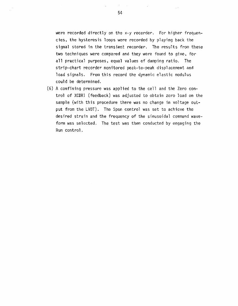
54
were recorded directly on the x-y recorder. For higher frequencies, the hysteresis loops were recorded by playing back thesignal stored in the transient recorder. The results from thesetwo techniques were compared and they were found to give, forall practical purposes, equal values of damping ratio. Thestrip-chart recorder monitored peak-to-peak displacement andload signals. From this record the dynamic elastic moduluscould be determined.
(6) A confining pressure was applied to the cell and the Zero control of XCDRl (feedback) was adjusted to obtain zero load on thesample (with this procedure there was no change in voltage output from the LVDT). The Span control was set to achieve thedesired strain and the frequency of the sinusoidal command waveform was selected. The test was then conducted by engaging theRun control.

CHAPTER 4
DYNAMIC PROPERTIES OF ICE UNDER CYCLICTRIAXIAL LOADING CONDITIONS
4.1 GeneralCyclic triaxial tests were carried out on two groups of laboratory
prepared samples of ice. In the first group the density ranged from0.900 to 0.908 glee; in the second group the density ranged from 0.767to 0.782 glee. It was felt that several parameters might influence thedynamic properties of ice. Hence, in addition to density the effects ondynamic properties caused by variations in temperature, confining pressure, strain amplitude, frequency, and number of cycles of loading wereinvestigated.
4.2 Test History Effects on Dynamic PropertiesAt the onset of the research program it was felt that the IItest
historyll a sample experienced might influence the dynamic propertiesmeasured. By test history is meant (1) the sequence in which the various physical parameters considered in the test pro9ram (temperature,confining pressure, frequency, strain amplitude, and number of cycles)were applied to the sample, and (2) the magnitude of the parameters considered following a given sequence. The results of the many tests conducted to establish an acceptable test history for a sample may be summarized as follows:
(1) Temperature - individual samples were tested through a range oftemperatures. It was found that the dynamic properties werecomparable to those of samples tested at a single temperatureif the samples were tested from high (-1°C) to low (-10°C) temperature. It was observed that if the sample temperature wasdecreased and it was allowed to readjust to the new temperaturefor a 24-hour period it would lIerasell any disturbance effectsthat might have occurred at the higher temperature. When thetests were performed from low (-10°C) to high (-1°C) temperature, the samples were disturbed, apparently at the coupling,even if they were left in the cell at a new test temperaturefor 24 hours prior to testing. The disturbance could be observed from the hysteresis loop. Melting between the samples
55

56
and the caps was found when the samples were taken out of thecell.
(2) Strain amplitude - the laboratory tests were conducted from lowto high strain amplitude at a given confining pressure. If thesample was retested at the lowest strain amplitude it was observed that the damping ratio of the later test was greater thanthe damping ratio of the former by about 50 percent. The dynamic Young's modulus appeared to be equal in magnitude.
(3) Confining pressure - when the samples were subjected to a highconfining pressure (greater than 100 psi) they deformed rapidly.The rate of deformation decreased with time and the volume ofthe samples appeared to decrease which would cause the densityto increase. This effect was demonstrated by testing a sampleat a low confining pressure, subjecting it to a high confiningpressure, then retesting at the low confining pressure. Thedynamic Young's modulus of the sample after it was subjected toa high confining pressure was slightly greater than the dynamicYoung's modulus of the sample before experiencing the high confining pressure. To avoid this problem the samples were subjected to the highest confining pressure (200 psi) used in thetest sequence for approximately 20 minutes before a test wasperformed. The rate of deformation of the samples was verysmall for subsequent applications of confining pressure afteremploying this procedure.
(4) Frequency - variations in the frequencies of testing (0.3, 1.0,and 5.0 cps) did not appear to cause sample disturbance.
(5) Number of cycles - the dynamic properties of the ice samplesdid not appear to be influenced by the number of cycles a samplewas subjected to provided the number of cycles of loading didnot exceed approximately 20 per one test. One sample was foundto be disturbed when it was subjected to more than 100 cyclesper one test. A sample subjected to about 150 cycles per onetest melted at the couplings and the dynamic Young's modulus wasfound to be very low.
An acceptable test history and the one used in the research programis shown in Figure 4.1. The range of test conditions was chosen to include the field conditions and loadings anticipated for frozen soil de-

57
Constant temperature
(sample subjected to an initial confining pressure of 200 psiprior to testing)
Approxima.te axial strain 3-3
x 10 %
__cp=200 ps~f=0.3 cps~f =1.0 cps~ f =5.0 cps
p=lOO ps:b,..-....e....f =0.3 cps.....-..-f=l.O cps~ f =5.0 cps
p= 50 ps:k-----.- f == 0 . 3 cps --+- f =1. 0 cps~f =5.0 cps
cp= 25 ps:b--+- f=O. 3 cps ----f;- f =1. 0 cps----.....f =5.0 cps
~cp= () psi--+-f=0.3 cps--... f =1.0 cps---....f =5.0 cps
')
A roximate axial strain = 9 x lO-~%
cp=200 psi---'-f=0.3 cps---...f=1.0 cps---+-f =5.0 cps
cp=lOO psi .. f=O. 3 cps -~~~f =1. () cps-...,. f =5.0 cps
t-......~p= 50 psi--....f=O. 3 cps~f =1. 0 Cp&s-.....~f =5.0 cps
cp= 25 psi---...... f =0.3 cps--......f =1. 0 cps::;..-.....jIbf =5.0 cps
Approximate axial strain = 2 x 10- 2%
t--....cp=200 psi---.... f =O.3 cps'---'iIl>of =1. 0 cps--"'f =5.0 cps
---'-"'Cp=lGO psi---+of=O. 3 Cps-"""l-....f =1. 0 Cpsl----4...... f =5.0 cps
Figure 4. 1 DIAGRAM OF ACCEPTABLE TEST HISTORY FOR ICE

58
posits subjected to strong motion earthquakes (Vinson, 1975). The rangeof specific test parameters are as follows:
(1) Temperature - the high density samples were tested at five temperatures (-1, -2, -4, -6 and -10°C); the low density sampleswere tested at three temperatures (-1, -4, and -10°C). A givensample was tested at one temperature only.
(2) Strain amplitude - the range of strain amplitude was approximately 3 x 10⁻³ to 2 x 10⁻²%axial strain. The maximum strainamplitude of testing at cp = 0 was limited to about 5 x 10⁻³%;at cp = 25 and 50 psi it was limited to about 9 x 10⁻³%; atcp = 100 and 200 psi it was limited to about 2 x 10⁻²%. Themaximum strain amplitudes were associated (approximately) witha tensile failure of the sample. (It was found that ice samples with the coupling described in Appendix B could be subjected to a tensile stress of about 80 psi.)
(3) Confining pressure - the high density samples were tested atfive confining pressures (0, 25, 50, 100 and 200 psi). At aconfining pressure of 0 psi, only a limited number of tests wereperformed at low strain amplitudes (2 x 10- 3 to 5 x 10- 3%). Thelow density samples were tested at four confining pressures (0,25, 50 and 100 psi). The low density samples were not tested atcp = 200 psi because the deformations associated with the application of this confining pressure were quite large. (The deformation of the low density samples under 200 psi confining pressure was greater than the range of the LVDT, ± 0.254 em.) At atemperature equal to -l~C, the maximum confining pressure waslimited to 50 psi, because of excessive deformations at 100 psi.A limited number of tests were performed at cp = 0 psi at lowstrain amplitudes, 3 x 10⁻³ and 5 x 10⁻³%.
(4) Frequency - in general only three frequencies of loading wereused in the test program: 0.3, 1.0 and 5.0 cps. A limited number of samples were tested at a very low frequency, 0.05 cps.
(5) Number of cycles - for each test condition a sample was subjectedto 20 cycles of loading.
Before a sample was subjected to the acceptable test history thecell pressure was increased to 200 psi for approximately 20 minutes. The

59
dynamic Young's modulus was evaluated at a strain amplitude of 9 x 10⁻³%
and a frequency of 0.3 cps. The value obtained from this test was compared to that obtained durinq the course of the test history as another
check on the disturbance of the sample. If they were found to be in good
agreement, the test was presumed to be acceptable. (For all the testresults reported herein the comparison was quite good.)
4.3 Influence of Number of Cycles on Evaluation of Dynamic PropertiesIt is generally felt by researchers conducting cyclic triaxial tests
on unfrozen soils that the dynamic properties associated with the 5th or
lOth cycle are the most appropriate for predicting ground response during
earthquakes. To assess the influence of the choice of the cycle number
on dynamic properties the variation of the ratio (E at Nth cycle/E at
lOth cycle) and (\ at Nth cycle/\ at lOth cycle) with number of cyclesat different frequencies, confining pressures, strain amplitudes, and
temperature was determined. These ratios are shown for high density iceat 1,5,10 and 20 cycles in Tables 4.1 and 4.2, respectively. There
appears to be no significant variation in dynamic Young's modulus withnumber of cycles for different frequencies, confining pressures, strainamplitudes, and temperatures. At the greatest, the dynamic Young's modulus at the Nth cycle is approximately 3.0% different from the modulusat the lOth cycle. Further, the damping ratio does not appear to varywith the number of cycles for different frequencies, confining pressures,
strain amplitudes, and temperatures. The damping ratio at the Nth cycleis at most about 10% different from the damping ratio at the 10th cycle.
The dynamic Young's modulus was evaluated from the load and dis
placement channels of the strip-chart recorder at the lOth cycle by measuring the peak-to-peak amplitude of the recorded waveform. The damping
ratio was evaluated from the hysteresis loop for the 10th cycle obtainedfrom the x-y recorder. Typical strip-chart and x-y recorder records areshown in Figure 4.2. The area of the hysteresis loop was determined witha planimeter. The error associated with this determination was estimatedto be approximately 5%.
4.4 Dynamic Young's Modulus of IceThe dynamic Young's modulus from the laboratory test program was
plotted against the log of axial strain amplitude expressed as a percent.

Table 4.1 VARIATION OF DYNAMIC YOUNG1S MODULUS OF HIGH DENSITY ICE WITH NUMBER OF CYCLES
E at Nth cycle
Temperature Axial strain Confining Frequency E at 10th cycle
( °C) amplitude pressure (cps)(%) (psi) Number of cycle1 5 10 20
-4 0.00287 50 0.05 0.988 1.003 1 0.995-4 0.00287 50 0.3 1. 035 1.014 1 1.020-4 0.00287 50 1.0 0.981 1.012 1 1. 024-4 0.00287 50 5.0 1.002 1.008 1 0.989
-4 0.00287 200 0.3 0.992 1.014 1 1.015 O'l0
-4 0.00287 50 0.3 1.035 1.014 1 1. 020-4 0.00287 0 0.3 1. 033 1.001 1 0.987
-4 0.00127 200 0.3 1.015 1. 038 1 1.063-4 0.00287 200 0.3 0.992 1. 015 1 1.014-4 0.0093 200 0.3 1. 005 1. 003 1 1. 005-4 0.0192 200 0.3 0.996 0.995 1 0.984
-1 0.00287 50 0.3 1. 000 1.008 1 1. 013-4 0.00287 50 0.3 0.992 1.015 1 1. 014
-10 0.00287 50 0.3 1.034 1. 011 1 1.019
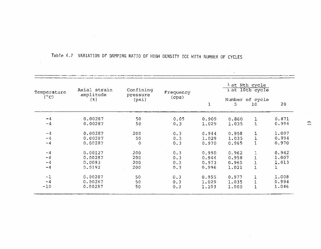
Table 4.2 VARIATION OF DAMPING RATIO OF HIGH DENSITY ICE WITH NUMBER OF CYCLES
Aat Nth cycle
Temperature Axial strain Confining Frequency A at 10th cycle
(0 C) amplitude pressure (cps)(% ) (psi) Number of cycle
1 5 10 20
-4 0.00287 50 0.05 0.909 0.860 1 0.871-4 0.00287 50 0.3 1. 029 1. 035 1 0.994 m
-4 0.00287 200 0.3 0.944 0.958 1 1. 007-4 0.00287 50 0.3 1. 029 1. 035 1 0.994-4 0.00287 0 0.3 0.970 0.965 1 0.970
-4 0.00127 200 0.3 0.990 0.962 1 0.942-4 0.00287 200 0.3 0.944 0.958 1 1.007-4 0.0093 200 0.3 0.973 0.965 1 1.013-4 0.0192 200 0.3 0.996 1.021 1 1
-1 0.00287 50 0.3 0.955 0.977 1 1. 008-4 0.00287 50 0.3 1. 029 1. 035 1 0.994
-10 0.00287 50 0.3 1.103 1. 000 1 1.046

Frequency (cycle/sec) .05 .3 5
enN
c
~:::I 1\ !\ ,rs A":'J:)
0 1 I \ I \ I \ I I1 \ Iii I"0Co
...J
":'
---cE o~ \ I \ I \ f 'lto ,) \ I \
U
.!! I \ I \ I \ I \Co - .0025 10 I (, 10 Ii ~
.!!!o
-.00051 V V V 1
a. Typical hysteresis loops(non-dimensional)
b. Typical load and displacement records
Figure 4.2 TYPICAL RECORDS OBTAINED DURING CYCLIC TRIAXIAL TESTING OF ICE

63
The plots are shown in Appendix C, Figures C.l to C.93 for the high density samples and Figures C.94 to C.126 for the low density samples. Eachplot represents a test condition associated with a specific frequency,temperature, and confining pressure. In general, the data from three (ormore) tests are available for each test condition.
For any given test condition there is "scatter" in the data points.It is believed that this was caused by:
(1) Slight variations of density of the samples which ranged from0.900 to 0.908 glcc for the high density samples and 0.767 to0.782 glcc for the low density samples.
(2) Slight differences in the structural composition of the samples,particularly near the coupling.
(3) Slight temperature differences between tests.(4) Loosening of the coupling between the samples and the cap and
base.(5) At the lower strain amplitudes of testing the test system ap
proached its limit of capability both electronically and mechanically. Some variations in test results at this extreme oftesting are to be expected.
Overall, however, it is felt that the data is reliable and provides agood basis for the interpretation of material properties.
4.4.1 Effect of Strain AmplitudeThe data presented in Figures C.l to C.126 in Appendix C suggests
that the dynamic Young's modulus of ice varies linearly with the log ofpercent axial strain amplitude, as least over the range of strain amplitude associated with the experimental program. The dashed lines in thefigures represent the least squares best fit line of the data. Theslopes of the least squares best fit lines vary slightly from one anotherbut do not appear to be influenced by frequency, confining pressure, ortemperature. The slopes of a few of the lines vary significantly fromthe majority of the lines because they are associated with only a limited number of data points. This is exemplified by Figures C.l, C.16,C.21, C.4l, C.61, C.66 and C.?? at a confining pressure of 0 psi and ata frequency of 0.05 cps.
Since the relationship between dynamic Young's modulus and the logof percent axial strain is not significantly influenced by other test

64
parameters it was assumed to be independent of the parameters. To establish the average least squares best fit line the dynamic Young's modulusfor all the experimental data ~was plotted against log of percent axialstrain amplitude, as shown in Figure 4.3 for the high density samples,and Figure 4.4 for the low density samples. The average slope is -0.0934(psi/log %) for the high density samples and 0.0067 (psi/log %) for thelow density samples. The average slopes indicate that the influence ofstrain amplitude for the high density samples is greater than for thelow density samples.
To assess the influence of frequency, temperature, and confiningpressure on the dynamic Young's modulus the average best fit leastsquares line was plotted through the data points for a given test condition. These are shown as solid lines in Figures C.1 to C.126. These1ines were drawn inte'rsecting the dashed 1ines at the "center" of thedata set for a given test condition. Obviously, personal judgment wasinvolved in this construction. The best fit least squares line throughthe center of the data set for given test conditions are summarized inFigures 4.5 to 4.23 for the high density samples and Figures 4.24 to 4.32for the low density samples. The figures shown the influence of confining pressure on dynamic Young's modulus at a specified temperature andfrequency. Dynamic Young's modulus varies from 340 x 103 to 900 x 103
psi for the high density samples and 260 x 103 to 600 x 103 psi for thelow density samples.
The relationship between dynamic Young's modulus and confining pressure, frequency, and temperature can be established by interpolation ofthe results presented in Figures 4.5 to 4.32 at a specified strain amplitude. In this chapter a strain amplitude of 4.4 x 10⁻³% (10g10 = -2.36)was selected for this purpose. Another strain amplitude could be selectedwithout changing the conclusions reached in Sections 4.4.2, 4.4.3, and4.4.4 owing to the fact that the variation between dynamic Young's modulus and log percent axial strain was assumed to be linear and independent of confining pressure, frequency, and temperature.
4.4.2 Effect of Confining PressureThe relationship between dynamic Young's modulus and confining pres
sure at an axial strain of 4.4 x 10⁻³%is shown in Figures 4.33 to 4.37for the high density ice and Figures 4.3~ to 4.40 for the low density ice.

LL0
en::>-'::>00::;:
'/""
'":=::>0>-u::;:«z z...., >-
c 0~ill
u ~ f-.... 0 V>ill LLa. -'w ::;en z0 :; ><~ «~
f- V>C
LL::>en
'" "".... f- w...., en :0-V> W
00 WU
'" enw
x "" >-« « f-::>CY enen zf-
wV>
0
1'5 3:0-'
'".;ill....:0en
LL
N,
COaM
I
oa
aoN
<l<l
ooM
<l
<1~
<l <l <l
<l
~~<l <11<1
<l ~<l~<1 <l <1 <l
<1
<l
a 0 0 0CJ a 0 a,...... \.Q l!1 ~
(~sd fOl) sntnpow S,fiunoA J~W~UAa
aaCO'"om
65
~<l ~lQ<l
uu"-en
"-"-
cO ~<;lj<5l<l>,....,
'" <l<lcQ.J <l-0
~a.E
~~~<l'" <l<l <lV>
ULLU0"-enV>
'" :30::>en
N 0a~<l<l <]<l <l "- 0
::;:
'";">, <l <l '-"....,
z
'" ::>0c >-ill
-0
~~
~~ '"...., ::;:
<l<l a c « za.ill zE
N U >- «'" , .... 0 ~V>ill f-a. ~ V>
0en LL -J0
W ::;Z x«
c -JV><.0
f-0') '" ::>
<l....
LLV>
<l N ...., es, V>f- :0-
';;; V>
~~W w
<lco
~<l<l x« V>w >-~ f-<::> V>
CO Cf Z<.0 V> W
N f-a
, V> :r:::i '-"-' :r:
':'"0 ill
0 ....M :0
en,LL
a a a a a a a a a0 a 0 a a a 0 a 0en 00 "- <D '" '" 0') N
Usd fa l) sntnpow s,6unoA J~W~UAa

66
_1.72
cp :: 0 ps i
cp = 25 ps i
cp " 100 psi
cP 50 psi
cp 200 psi
Sample density'" 0.904 giee
_2.36 _2.04
Strain (109 percent)
Figure 4.6 OYNAl1lC YOUNG'S I~OOUlUS ~£RSUS AXlAl STRA1N FOR HIGH
OENSl1 i ICE AT _1°C A@ 0.3 CPS
980.
900.
820.
740.
~
P-
M0
660.~
""~0:>:
:"580.
O'
""?-u 500 ..~
B
420.
340.
260.
-3.00_2.68
t\xiol
Cp" 25 psi
ep " 200 psi
ep " 50 psi
ep " 100 ps I
Sample density" 0.904 glee
_2.68 _2.36 -2.04
Axial strain (log percent)
Fi9ure
4.5 OYNAMIC YOUNG'S 1400ULUS VERSUS AXIAL STRAIN FOR HIGH
OENSITY ICE AT _l'C AND 0.05 CPS
L-l_---I------~---L.-----.-J--1.72
980.
goo.
820.
740.
c..
M0
';660.
~
'is'",n SBO.~
c00~
u.~ 500.
"~
420.
340.
260.
_3.00
_1.72
cp=25 pSl
cp :: SO p'S i
S3mple density'" 0.904 glee
Cp" 100 psi
cp = 200 psi
_2.36 _2.04
A;dal strain (log pHcent
)
Figure 4.8 DYHAIo\IC YOUNG'S MODULUS VERSUS AXIAL STRAIN FOR HIGH
DEHSITY ICE AT _1°C AND ••0 CPS
980.
900.
820.
740.~
0-
M
'"::::.~
660.
""~~ 580.'g'
~u
.~ 500.
B
420.
340.
260.
_3.00-2.68
_1.72
cp 50 psi
cp " 0 psi
ep 200 psi
cp 25 psi
ep " 100 psi
sample density" 0.904 9/ee
.2.68 _2.36 _2.04
I\x.ial Strain (1og percent)
Figure 4.7 OY1lAI'\lC YOUNG'S IoIOOOLUS VERSUS AXIAL STRAIN FOR HIGH
DEHSl1Y ICE AT -1'C AHD 1 .0 CPS
\)1\0.
900.
820.
740.~
P-
M :::~ 660.0
~
~
~
-~ ,SO.O'
""0~
u
.~ 500.>,
'"420.
340.
260.
_3.00

_1.72
cp o 2Spsi
cp " 0 psi
cp 100 pS1
cp " 50 ps i
cP 200 psi
Sample density 0 0.904 g/ce
_2.68 -2.36 _2.04
Axial Stra;tt (109 percent)
figure 4.10 D~NAl'IIC ~OUNG'S \.\OOUlUS VERSUS AXIAL STRAIN FOR HIGH
DENS!T~ ICE AT _2°C AND 0.3 CPS
67
980.
900.
820.
740.
~0-
M0
~
660.0>
~
"0
~
::' 580.
g;?u
.~ 500.
>,co
420.
340.
260. -
_3.00
-1.72
cp _ 100 psi
cp 50 psi
cp " 25 psi
cp " 200 psi
Sample density· 0.904 g/ec
-2.68 -2.36 _2.04
Axial Strain (log percent)
fl9ure
4.9 D~NAMIC ~OUNG'S r~OOUlOS VERSOS AXIAL STRAIN fOR HIGH
DENSITY ICE AT _2°C AND 0.05 CPS
980.
900.
l\(.O,
~
740.0-
00
e:-~ 660 .0>
:g0,;:
~ 580.~
0>0>u
~ 500.c1';
420.
340.
2&0.
_3.00
Sample density'" 0.904 glee
-1.72
cp ;: 50 psi
cp ;: 200 psi
cp '" 100 psi
cp '" 25 ps i
-1.68 _2.36 _2.04
Axial Strain (109 percent)
Figure 4.1Z oYKAl'IIC ~OUKG'5 110DULUS VER5U5 AXIAL STRA:" FOR K1Grl
DEKS!T~ ICE AT _ZoC AKD 5.0 CP5
980.
900.
820.
~ 140.0-
M0
~ 660.0>
~::''"!
580.
w.~
c 500.Ei
4Z0.
340.
Z60.
_3.00
Sample density 0 0.904 glee
cp \00 psi
cp " 200 psi
Cp o 25ps i
cp " 0 psi
cp 50 psi
-Z .68 -Z. 36 -Z. 04
Axial strain (log percent)
Figure 4.11 O~NI\t\lC ~OUKG'S MODULUS VERSUS AXIAL STAAIK fOR HIGH
OEK51"TV lCE AT _ZoC MO i ,0 CP5
980.
900.
820.
~
740.0-
M0
~ 660."0>
~::'§ 580.
;?w
.~ 500.i;;
420.
340.
260.
_3.00

_1.72
cp • 50 psi
cp = a ps i
ep 25 psi
ep = 100 psi
Samp1e density"" 0.904 glee
_2.68 _2.36 _2.04
Axial Strain (log percent)
Figure 4.14 OYNAMIC YOUNG'S flOOULUS VERSUS AXIAL STRAIN ,OR HIGH
DENSITY ICE AT _4°C ANO 0.3 CPS
68
980.
900.
8Z0.
140.0P-
MO
0660.
~
~
"00:E
-~ ;'80.g'
~u.\ ;'00.
C>
420.
340.
Z60.
_3.00
cp = 100 psi
cp=Z;,psi
cp - ;'0 psi
ep = ZOO psi
Sample density· 0.904 9/ee
-Z.68 _2.36 -2.04
Axial Strain (log percent)
fIgure 4.13 OYNAIUC YOUNG'S MOOULUS ~ERSUS ~XI~L STR~IN FOR HIGH
OENSITY ICE AT -4"C ANO 0.05 CPS
980.
900.
820.
740.
~
"'0::.
0 660.~
~
."g~ ;'80.¥;;:u
.~ 500.
S
4Z0.
340.
260.
_3.00
Sample density 0.904 glee
_1.72
Cp=,25psi
cp 50 psi
cp =' 0 psi
ep 100 psi
cp 200 psi
_2.68 _2.36 -2.04
Axial Strain (log percent)
figure 4.16 oYNAAIC yOUNG'S fIOOULUS VERSUS AXIAL STRAIN FOR HIGH
OENSITY ICE liT _4"C IINO $.0 CPS
980.
900.
820.
740.~
P-
M :::~
660.~
~f~
-g> 580.~
~u'Ii 500.~S
420.
340.
280.
_3.08
-1.72
Sample density· 0.g04 g/cc
cp = 25 psi
Cp = 100 psi
cp • 0 psi
cp • 200 psi
cp • 50 psi
_2.68 _2.36 -2.04
Axial Strain (lOg percent)
figure 4.15 OYNAAIC YOJNG'S f'OOULUS ~ERSUS ~XIAL STRAIN fOR HIGH
OENSITY ICE AT -4"C AND).O CPS
980.
900.
820.
740.
0P-
M0
0660.
~
~~
~ 580.~
<0~0~
u
'Ii 500.~iJ
420.
340.
260.
_3.00

-1. JZ_2.04
ep 200 psi
cp 100 PSl
ep 50 psi
ep - 25 psi
_2.36
sample density" 0.904 9/ ee
Axia1 Strain {log percent)
Figure 4.18 DYNA!.\lC YOUNG'S MOOllLUS VERSU5 AXIAL STRAIN FOR HIGH
DENSITY ICE AT -6'( AND 1.0 CPS
69
980.
900.
820.
'"740.
~
'"0
'" 660."S'd
f'"-", 5S0.S:;.u'E~
500.
'"
420.
340.
260.
_3.00_2.68
-1.72
ep " 25 ps i
ep " 100 pS1
ep = SO ps i
cp = 200 psi
sample density" 0.904 glee
-2.04
Axial Strain (109 percent)
Figure 4.17 DYNAMIC YOUllG'S MODULUS VERSUS AXIAL STRAIH FOR HIGH
DENSlTY ICE AT -6'C AND 0.3 CPS
980.
900.
d/O.
740.
'"a-M
;!.
'!lhh\).
:;
i!' 1.1(10.
Iu
i 1.lnu ..;.
4m.
',40.
260.
_3.00_2.68 -2.36
Sample density" 0.904 glee
-2.04
cp - 200 psi
cp - 100 pSl
cp - 50 psi
ep - 25 psi
_2.36sttain t109 percent)
Figure 4.19 DYNJ\HIC YOUNG'S MOOULUS VERSUS AXIAL SWAIN fOR HIGH
DENSlTY ICE AT -6·C AND 5.0 CPS
9BO.
goO.
B20.
740.
'"~M::. 660.
'!l
"'"0'"!' SIlO.0>
§:;.u.~ 500 .
"l'!420.
340.
260.
_3.00_2.68
Ax i a1

70
cp = 100 pSl
cp::::Opsi
cp = 25 ps i
cr • 50 ps i
cp = 200 psi
Sample density 00.904 glce
_2.68 -2.36 -2.04
Adal Strain (109 percent)
Figu," 4.21 OYNAI'\\C YOUNG'S i'\OOUlUS VERSUS AXIAL STRAIN FOR HIGH
OENSl1Y ICE AT -lO'C AND 0.3 CPS
980.
900.
820.
~ 740.
p.
co
::-'!l
660.
.iJg
'" 580.0>§~u.~ 500 .
"1]
420.
340.
Z60.
_3.00
-1.72
cp • 200 psi
cp 100 psi
cp • 25 psi
cp = SO psi
Sa",ple density· 0.904 g/ce
-2.6~ _2.36 _2.Q4
A<ial Strain (log pe<cent)
Figure 4.20 DYNAMIC YOUNG'S II0DUlUS VERSUS AXIAL SWAIN FOR ~IG~DENSl1Y ICE Al _10°C AND 0.05 CPS
9~Q.
900.
112O.
740·
'"<,.
Cl
;::
'"660.
~
.iJ;'7.,
:' 5~0.
g'
"0r".~ 500.
6:
420.
340.
(60.
_3.00
Sall"lple density'" 0.904 glee
cp = 25 psi
cp = 200 psi
cp 100 psi
ep :::: 0 psi
c:p 50 psi
_2.36 -2.04
Axial strain {lOg percent)
figu," 4.23 DYNPJoIIC YOUNG'S IWOUlUS VERSUS MIAl STMIN FOR HIGH
DENSITY ICE AT _10°C AND 5.0 CPS
980.
gOO.
820.
v'740.
p.
no::.'" 660."~~
'"-0' S8Q.S~u
"e.. 500.~
420.
340.
260.
_3.00_2.68
_1.72
cp "' ioo pSI
cp=SOpsi
cp = 200 psi
cp :::: 0 psi
cp := 25 psi
Sample density· 0.g04 g/cC
_2.68 _2.36 _Z.04
Axial Strain (log percent)
Figure 4.22 DYNPJoIIC YOUNG'S MODULUS VERSUS AXIAL SJMIN FOR ~IG~DENSITY ICE Al _10°C ANO '.0 CPS
930.
gOO.
320.
HO.
'"o·n
::-'!l 660.
~i't:
~c' 580.~~
~
".~SOD.
";;;
420.
340.
260.
_3.00

71
Figure 4.24 DYNAHIC YOUNG'S HODULUS VERSUS AXIAL STRAIN FOR LOW
DENSITY ICE AT _1°C AND 0.3 CPS
Axial Strain (log percent)
Sdlllple density, 0.77 glee
-2.12
cp 25 psi
cp 50 psi
cp 0 psi
Sample density" O.}I
-308 -276 -244
Axial Strain (log percent)
Figure 4.25 DYNAI~IC YOUNG'S HODULUS VERSUS AXIAL STRAIN FOR LOfI
DENSITY ICE AT - 1°C AND 1.0 CPS
740.
660.
580 .
.~i'l
M
::. 500.
~
0u~
420.~
0>000
u 340 ..~
~
260.
180.
IDa.
-3.40-2. 12-2.44
cp 0 psi
cp 25 ps i
cp 50 psi
-2.76-3.08-3.40
I~().
100.
5S0.
IBO.
&r.o.
260.
.~ 340.
~/1'
o
~
"o;" ~20.
~
Mo:::. 500.
cp =: 50 ps i
CP=25ps;
Sample density'" 0.77 glee
740.
660.
580.
~
Ma
5DO.
~0
u,J£
420.v,0>000>u 340.
!B
260.
180.
100.
-3.40 -3.08 -2.76
cp =: a psi
-2.44 -2.12
Axial Strain (log percent)
Figure 4.26 DYNAMIC YOUNG'S MODULUS VERSUS AXIAL STRAIN FOR LOW
DENSITY ICE AT -JoC AND 5.0 CPS

72
Axial Strain (log percent)
Figure 4.28 OYNAfllC YOUNG'S I·IOOULUS VERSUS AXIAL STRAIN FOR LOW
DENSITY ICE AT -4"C AND 1.0 CPS
Sample density.::. 0.77 glee
740. 740.Samp Ie dens ity , 0.77 g/cc
bbl1. 660.
~) :{O .580.
0.(l
M0
1),10.cp 100 psi 500.
"0 cp 50 ps i ~u cp 25 psi 00
u:-;:0
410. '" 420.~
c~0c0 cp 0 psi 0
~u
u2 340.
.~340.
;;;;;;
260. 260.
IBO. 180.
100. 100.
-3.40 -3.08 -2.76 -2.44 -2.12 -3.40 -3.08Axial Strain (log percent)
Figure 4.27 DYNAMIC YOUNG'S I~OOULUS VERSUS AXIAL STRAIN FOR LOW
DENSITY ICE AT _4°C AND 0.3 CPS
-2.76
cp 100 ps icp 50 ps 1
cp " 25 ps i
cp 0 psi
-2.44 -2.12
cp " I DO psi
cp - 50 psicp " 25 psi
cp " 0 psi
Sample dens ity :< 0.77 glee
-3.08 -2.76 -2.44 -2.12
Axial Strain (log percent)
Figure 4.29 DYNAMIC YOONG'S MODULUS VERSUS AXIAL STRAIN FOR LOW
DENSITY ICE AT -4°C AND 5.0 CPS
740.
660.
580.~
0.
M0
~500.
0
0u0
'"-~. 420.~
c~
0>u
.~ 340.
;;;
260.
180.
100.
-3.40

73
Axial Strain (log percent)
Sample density", O. 77 ~l/cc
Axial Strain (log percent)
-2.12-2.44
cp 0 100 psicp 0 50 ps i
cp '=' 25 ps i
cp 0 0 psi
-2.76-3.08
740.
660.
580.
~
aM
0
:::: 500.~~
'0
:it420.
~
c~0ru
.~ 340 .
6'
260.
180.
100.
-3.40-2.12-2.44
cp 0 100 psicp 0 50 psi
cp 0 25 psi
cp - 0 psi
-2.76
7411.
660.
580.
~
aM
0
500.~~
'00;;.-::
-~420.
~.
c~
0
u
.~ 340 .
i~'
,611.
IBO.
100.
-3.40 -3.08
Figure 4.30 DYNAfIIC YOUNG'S i100ULUS VERSUS AXIAL STRAIN FOR LOW
DENSITY ICE AT _10°C AND 0.3 CPSFigure 4.31 DYNAMIC YOUNG'S NODULUS VERSUS AXIAL STRAIN FOR LOW
DENSITY ICE AT _10°C AND 1.0 CPS
740.
660.
580.
~
aM
0
:::: 500.~~
u0
" 420.~
c
§u
.~ 340 .
6'
260.
180.
100.
-3.40
Sample density 0.77 glee
cp 0 100 psicp - 50 psi
cp 0 25 ps icp 0 0 psi
-3.08 -2.76 -2.44 -2.12
Axial Strain (log percent)
Figure 4.32 DYNAMIC YOUNG'S ,mOULUS VERSUS AXIAL STRAIN FOR LOW
DENSITY ICE AT -lOoC AND 5.0 CPS

Fi gure 4,34 DYNAMIC YOUNG'S MODULUS VERSUS CONF IN ING PRESSURE
FOR HIGH DENSITY ICE AT -2"C
Frequency
l::. 0,05 cps
A 0,3 cps
.A. 1,0 cps
.. 5,0 cps
Sample density;; 0.904 glee
Axial strain = 4.4xlO-3%
75 iOO 125 150 175 200
Confining Pressure (psi)
5025
74
F,'equency Sample density;; 0.904 glee
l::. J.05 cps Axia 1 strain = 4.4xl0- 3%
A 0.3 cps-!,1(I. gOO.
A. I. ° cps
A -J.O cps
<120, 820,
140, 740,~
n0.
M0
0 =---:. 660.~
660,~
0~
."~
0 ~
52,0, -~ 580,~
~~
~~
0 00 >->- u
500. .~ 500,~
~ BB
420, 420,
340. 340,
260, 260,
25 50 75 100 125 150 175 200
Confining Pressure (psi)
Figure 4,33 OYNAI4IC YOUNG'S I-IODULUS VERSUS CONFINING PRESSURE
FOR HIGH DENSITY ICE AT -1 "C
gOO,
820,
740.
0.
0
660,
~
0~0
'"-~
580,~
~
0>-u
500,.~
B
420,
340,
260.
Frequency
A 0,05 cps
A 0.3 cps
A. 1.0 cps
A 5.0 cps
Samp 1e dens ity '" 0.904 g/cc
Axial strain = 4.4xlO-3%
gOO,
820,
740,
660,
_~ 580,
SOD,
420,
340.
260,
Frequency
A 0,3 cps
.A. I,D cps
A 5,0 cps
Sample density ~ 0.904 glee
Axial strain := 4.4xlO-3%
75 100 125 150 175 200
Confining Pressure (psi)
5025
Figure 4.36 DYNAI-lIC YOUNG'S MOOULUS VERSUS CONFINING PRESSURE
FOR HIGH OENSITY ICE AT -6"C
5025 75 100 125 150 175 200
Confining Pressure (psi)
Figure 4.35 OYNAlHC YOUNG'S MODULUS VERSUS CONFINING PRESSURE
FOR HIGH OENSITY ICE AT -4"C

900.
260.
Frequency
LI. 0.05 cps
A 0.3 cps
A 1.0 cps
• 5.0 cps
Sample density" 0.904 9/cc
Axial strain = 4.4x10- 3%
75
740.
660.
580.
0.
M0
500.~
~
~
'C0
"-~ 420.
§~
u.~ 340.
~
260.
180.
100.
Frequency
A 0.3 cps
A 1.0 cps
• 5.0 cps
Sample density::: 0.77 g/ee
Axial strain'" 4.4xl0- 3t
25 50 75 100 125 150 175 200
Confining Pressure (psi)
25 50 75 100 125 150 175 200
Gonf; ni ng Pressure (ps i)
Fi9ure 4.37 DYNAMIC YOUNG' S I~ODUlUS VERSUS CONFINING PRESSURE
FOR HIGH DENSITY ICE AT -lDoC
Figure 4.38 DYNAMIC YOUNG'S f.lODUlUS VERSUS CONFINING PRESSURE
FOR lOW DENSITY ICE AT -1°C
740.
660.
580.
0.
Ma
500.
~~
'C0
" 420.-~
'"c~
0>u 34D..~;;,
260.
Frequency
A 0.3 cps
A 1.0 cps• 5.0 cps
Sample density" 0.77 glcc
Axial strain'" 4.4xlO- 3%
740 .
660.
580.~
0.
Ma
~
500.
""'C~
-~ 420.
'"c"~u's 340 .
~
260.
Frequency
A 0.3 cps
A 1.0 cps
• 5.0 cps
Sample density", 0.77 glee
Axial strain = 4.4xlO- 3%
Confining Pressure (psi)
Figure 4.39 DYNAMIC YOUNG'S I<tODUlUS VERSUS CONFINING PRESSURE
FOR lOW DENSITY ICE AT -4'C
Figure 4.40 DYNAMIC YOUNG'S MODULUS VERSUS CONFINING PRESSURE
FOR lOW DENSITY leE AT _lDoe
180.
100.
25 50 75 100 125 150 175 200
180.
100.
25 50 75 100 125 150 175 200
Confining Pressure (psl)

76
The relationship is, in general, plotted at four frequencies for a given
temperature. The data at five temperatures (-1, -2, -4, -6 and -10°C)was available for the high density ice, and at three temperatures (-1,-4 and -10°C) for the low density ice.
The results shown in Figures 4.33 to 4.37 indicate the dynamicYoung's modulus of high density ice increases with increasing confiningpressure (1) gradually from a to 25 psi (approximately 8%), (2) steeplyfrom 25 psi to 50 psi (approximately 20%), (3) gradually from 50 psi to100 psi (approximately 8%), and only slightly from 100 psi to 200 psi.Temperature and frequency do not appear to have a significant influenceon the relationship between dynamic Young's modulus and confining pressure.
The dynamic Young's modulus of low density ice at temperatures of-1 and -4°C increases rapidly with increasing confining pressure from 0to 25 psi (approximately 14%). At a temperature of -10°C, the rate ofincrease in this range of confining pressure is gradual and comparable tohigh density ice. The dynamic Young's modulus increases gradually forall test temperatures with increasing confining pressure from 25 psi to50 psi; it is almost constant with increasing confining pressure from 50psi to 100 psi. Frequency does not appear to have an influence on therelationship between dynamic Young's modulus and confining pressure.
The relationship between dynamic Young's modulus of ice and confininf pressure might be caused by changes in the microstructure of the iceunder various confining pressures. Microfissures might close when a sample is subjected to a high confining pressure. This would lead to a sample with a higher dynamic modulus. Conversely, they might open when asample is subjected to a lower confining pressure which would lead to alower dynamic modulus. This tendency was exemplified by the fact thatwhen the confining pressure was released from the triaxial cell and thesample was not allowed to deform there was a gradual increase of load onthe sample. This load might be associated with the elastic rebound characteristics of the microfissures.
4.4.3 Effect of FrequencyThe relationship between dynamic Young's modulus and frequency at
an axial strain of 4.4 x 10⁻³%is shown in Figures 4.41 to 4.45 for highdensity ice and Figures 4.46 to 4.48 for low density ice. The re1ation-

Figure 4.41 DYNAI·lIC YOUNG'S I~ODULUS VERSUS FREQUENCY FOR HIGH
DENSITY ICE AT _1°C
Sample density 0 0.904 9/ee
Axial strain" 4 4xlO- 3%
77
C.onfining pressure Sample density:::: 0.904 9/ee
Ii psi Axial stra in " 4 4xl0- 3%
900. A 25 psi
A 50 psi
'" 100 psi820.
A 200
740.
~
0-
M0
660.~
"i~
~580.
-~C>~~
0>u 500..~
6:
420.
340.
260.
0.05 0.3 1.0 5.0
Frequency (cps)
Fi9ure 4.42 DYNAMiC YOUNG'S MODULUS VERSUS FREQUENCY FOR HIGH
DENSITY ICE AT _2°C
5.01.00.3
Frequency (cps)
0.05
Confi ning pressure
A D psi
A 25 psi
A 50 psi
260.
340.
900.
740.
420.
820.
~ 0110.
'g 660.
" oDD.
B
"o>.
Fi gure 4.44 DYNAMIC YOUNG'S !'ODULUS VERSUS FREQUENC Y FOR HIGH
DENSITY ICE AT _6°C
Confining pressure
5.0
Sample density::: 0.904 glee
Axial strain = 4.4xlO- 3i;
0.3 1.0
Frequency (cps)
0.05
A 25 psi
A 50 psi
.&. 100 psi
A 200 psi
Confining pressure Samp 1e dens; ty o 0.904 gleeA o psi
4.4xI0- 3%Axial stra in "900. A 25 psi 900.
A 50 ps i
'" 100 ps i820. A200 psi 820.
740. 740.
0- 0-
M Mco 0~
~660. ., 660.
~ 0
0 0'0
~:i!-~ 580. -~ 580.~. 0-~ ~~ 00> ~u u
~500. " 500.
;gB B
420. 420.
340. 340.
260. 260.
0.05 0.3 1.0 5.0
Frequency (cps)
Figure 4.43 DYtl'\MIC YOUNG'S I-I)DULUS VERSUS FREQUENCY FOR HiGH
DENSITY iCE AT _4°C

900.
820.
'8. 740.
~
'~ 660.
>:
mc~ IjHO.
78
740.
660.
~
~
(Vb 580.
.g 500.>:
mc~
;: 420.
Confini ng Pressure
A 0 psi
J:>. 25 psi
A 50 psi
Sample density'" 0.77 glee
Axial strain 4.4xlO- 3;
4,0.
·i40.
260.
Confining pressure
A psi
J:>. 25 psi
A 50 psi
" 100 psi
& 200 psi
Sample density'" 0.904 glee
Axial strain ~ 4.4xI0- 3%
340.
260.
180.
100.
0.05 0.3
Frequency (cps)
1.0 5.0 0.05 0.3
Frequency (cps)
1.0 5.0
Figure 4.45 DYNAMIC YOUNG'S MODULUS VERSUS FREQUENCY FOR HIGH
DENSITY ICE AT -lOoC
Figure 4.46 DYNA;'lIC YOUNG'S 1·100UlUS VERSUS FREQUENCY FOR LOW
DENSITY ICE AT -I 'C
740.
660.
580.~
Me
:::.~ 500.~
~
0
"I 420.
u.~
~ 340.
260.
ISO.
100.
Confining pressure
~ psi
J:>. 25 ps i
A 50 psi
AIOO psi
Sample density 0 0.77 g/ee
Axial strain::: 4.4xlO-3%740.
660.
580.
~
Me
:::. 500.~
~
~
~_~ 420.mc~
~u
.~ 340.
l5'
260.
180.
100.
Confining pressure
A 0 psi
J:>. 25 psi
A 50 psi
A 100 psi
Sample density" 0.77 glee
Axial strain - 4.4xlO- 3X
0.05 0.3
Frequency (cps)
1.0 5.0 0.05 0.3
Frequency (cps)
1.0 5.0
Figure 4.47 OYNAI1IC YOUNG'S MODULUS VERSUS FREQUENCY FOR lOW
DENSITY ICE AT _4°C
Figure 4.48 OYNAHIC YOUNG'S MODULUS VERSUS FREQUENCY FOR LOW
DENSITY ICE AT -10°C

79
ship is, in general, plotted at five confining pressures for a giventemperature.
The dynamic Young's modulus of high density ice increases rapidly(approximately 20%) for an increase in frequency from 0.05 to 0.3 cps.Between 0.3 and 5.0 cps the rate of increase is, in general, not as rapid.The increase of dynamic Young's modulus with frequency appears to begreater for higher temperatures (-1°C) than for lower temperatures (-10°C).Confining pressure does not appear to have an influence on the relation~
ship between dynamic Young's modulus and frequency.No tests were performed at a frequency of 0.05 cps on the low den~
sity ice samples. The dynamic Young's modulus of low density ice increasesapproximately 4% for an increase in frequency from 0.3 to 5 cps. For samples at a temperature of -1 and -4°C the rate of increase is greater inthe frequency range 0.3 to 1.0 cps than in the range 1.0 to 5.0 cps. Forsamples at a temperature of -10°C, the relationship between dynamic Young'smodulus and frequency is almost linear in the range 0.3 to 5.0 cps. Confining pressure does not appear to have an influence on the relationshipbetween dynamic Young's modulus and frequency.
4.4.4 Effect of TemperatureThe relationship between dynamic Young's modulus and temperature is
shown in Figures 4.49 to 4.52 for high density ice and Figures 4.53 to4.56 for low density ice. The relationship is, in general, plotted atfour frequencies for a given confining pressure.
The dynamic Young's modulus of the high density ice increases withdecreasing temperatures. At a confining pressure of 25 psi the modulusincreases approximately 20% for a temperature decrease from -1 to -4°C.It also increases approximately 20% for a temperature decrease from -4to -10°C. The modulus increases more rapidly in the temperature range-1 to -4°C than in the temperature range -4 to -10°C. For the temperature range -4 to -10°C, the rate of increase is almost constant. At lowconfining pressures, the rate of increase is slightly greater than athigh confining pressures. The frequency of testing appears to have nosignificant influence on the relationship between dynamic Young's modulus and temperature.
The dynamic Young's modulus of low density ice increases approximately 35% for an increase in temperature from -1 to -4°C and approxi-

80
Frequency
~ 0.05 cps
Sample density" 0.904 9/ee
Axial strain = 4.4xlO- 3%
0>C
a~
u
.~
B
iHlIl.
740.
660.
580.
500.
420.
340.
~
A 0.3 cps
A 1.0 q)S.. 5.0 cps
900.
820.
740.
~
~
M0
660.
~
~
~
-0a
:;::580.
-~0>C~
a>u 500..§
~
B Frequency
420. ~ 0.05 cps
A 0.3 cps
41.0 cps340.
... '.0 cps
Sample density'" 0.904 glee
Axial strain = 4.4xl0- 3'1,
260. 260.
-10-9-8-7-6-5
Temperature ("C)
-4-3-2-1
Figure 4.50 DYNAHIC YOUNG'S 11DDUlUS VERSUS W1PERATURE FOR HIGH
DENSITY ICE AT A CONFINING PRESSURE OF 50 PSI
-10-9-8-7-3-2-1 -4 -5 -6
Temperature (OC)
Fi9ure 4.49 OYNAMIC YOUNG'S MOOUlUS VERSUS TEflPERATURE FOR HIGH
OENSITY ICE AT A CONFINING PRESSURE OF 25 PSI
900.
820.
740.
~
~
MC>
::. 660.
~~
-0a
'" 580.0>c~
a~
u500..§
>,C>
420.
340.
Frequency
~ 0.05 cps
A 0.3 cps
A 1.0 cps
... 5.0 cps
Sample density. 0.904 glee
Axial strain = 4.4xlO-3%
900.
820.
740.
"M
:::660.
~=j
580.-:!'§u
500.i~
420.
340.
Frequency
~ 0.05 cps
A 0.3 cps
4 1.0 cps
... 5.0 cps
Sample den:.ity :.: 0.904 glee
Axial strain = 4.4xlO- 3%
~O. ~O.
-1 -2 -3 -4 -5 -6 -7 -8 -g -10 -1 -2 -3 -4 -5 -6 -7 of, -9 . J(}
Temperature COe) Temperature ('C)
Figure 4.51 DYIlAMIC YOUNG'S 110DUlUS VERSUS TEMPERATURE FOR HIGH
DENSITY ICE AT A CONFINING PRESSURE OF 100 PSI
Fi9ure 4.52 DYIlAMIC YOUNG'S MODULUS VERSUS TEMPERATUR[ FOR HIGH
DENSITY ICE AT A CONFINING PRESSURE OF 200 PSI

81
rrequenCj Sample density 0.77 glee Salilple dens i ty 0.77Frequency q/ce/·10.
60 3 4xI0- 3%740.
cps Axia 1 stra in 0 A 0.3 cps Axia 1 strain 4 . 4xl 0- -.l~',
Al .0 cps Al .0 cps
A'j .0 CP',45 0
!lbO, 660. cps
~;W. 580.
r-, 0-
", M0 0
Il)O. ::. 500.
., ~
~
0~
'00 a
:;: :;:420.420.
rn rnc c~ ~
0 a>-
u 340. u 340.
~ ~2;' B
260. 260.
FJO. 180.
100. 100.
-I -2 -3 -4 -5 -6 -7 -8 -9 -10 -I -2 -3 -4 -5 -6 -7 -8 -9 -10
Tempera ture ( "C) Temperature ( 'C)
Fiqure 4.53 DYNA,IIC YOUNG' 5 I~ODULIiS VERSUS TElWERATURE FOR LOW Figure 4.54 OYNAI1JC YOUNG'S 140DOLUS VERSUS TEi-iPERATURE FOR Lm~
D[NSITY ICE AT A CONF JNJNG PHESSIiHE OF G PSI DENSITY ICE AT A CONFIN ING PRESSURE OF 2S PSI
Temperature (Oe)
Figure 4.56 OYNA!'IIC YOUNG'S MODULUS VERSUS TEIIPERATURE FOR LO::
DENSITY ICE AT A CONFINING PRESSURE OF 100 PSI
Frequency
- 10-g-8-7
Sarnple density'" 0.77 glee
Axial strain::: 4.4xl0- 3%
-6-5-4-3
60.3 cps
A 1.0 cps
.... 5.0 cps
-2-I
500.
660.
740.
580.
420.
340 .
260.
180.
100.
rnc~
a
u
.~
B
Mo
Frequency Sampl e dens Hy '" 0.77 glee
6 0.3 cps Axial strain :0 4.4xlo- 3%740. A 1.0 cps
'" 5.0 cps
660.
580.
0-
Ma::. 500.
~0
'0a
'" 420.-~rnca>-
.~340.
B
260.
180.
100.
-I -2 -3 -4 -5 -6 -7 -8 -9 -10
Tempera ture (OC)
Figure 4.55 DYNAIIIC YOUNG'S i,ODULUS VERSUS THIPERATURE FOR [OW
DENSITY ICE AT A CONFINING PRESSURE OF 50 PSI

82
mate1y 20% for an increase in temperature from -4 to -lOoe. The modulusincreases almost linearly in the temperature range -4 to -lOoe. The rateof increase is smaller than for the temperature range -1 to -4°e. Frequency and confining pressure appear to have no significant influence onthe relationship between dynamic Young's modulus and temperature.
4.4.5 Effect of DensityThe results presented by Roethlisberger (1972) and Bennett (1972)
indicate that the dynamic elastic properties of ice vary linearly withdensity in the range 0.7 to 0.919 glcc (refer to Figures 2.11,2.12, and2.13, Section 2.3.2). In the research program the dynamic Young's modulus was evaluated at two densities: 0.77 and 0.904 g/cc. The relationship between dynamic Young's modulus and density was assumed to be linear.The relationship is shown in Figures 4.57 to 4.59 for three frequenciesat a confining pressure of 50 psi, axial strain of 4.4 x 10⁻³%, and agiven temperature. In Figures 4.60 to 4.62 the relationship between dynamic Young's modulus and density is shown for three confining pressuresat a frequency of 1.0 cps, axial strain of 4.4 x 10⁻³%, and a given tem
perature.The dynamic Young's modulus increases approximately 60% as density
increases from 0.77 to 0.904 g/cc. Temperature, frequency, and confiningpressure do not appear to have a significant influence on the relationship.
4.5 Damping Ratio of IceDamping ratio was plotted against the log of axial strain expressed
as a percent as shown in Appendix D, Figures 0.1 to 0.19, for the highdensity ice samples and Figures 0.20 to 0.28 for the low density ice.The range of damping ratio is from 0.001 to 0.14 for the high densityice and from 0.001 to 0.10 for the low density ice.
For a given test condition considerable "scatter ll exists in thedata. Several reasons for this scatter are given in Section 4.4. Inaddition to these reasons it is also felt that II scatter" occurred inmeasurements of damping ratio owing to personal error in the measurementof the area of the hysteresis loop.
As a consequence of the II scatter ll in the data there appears to beno identifiable relationship between damping ratio and confining pressure

83
Frequency Confining pressure::: 50 psi
Frequency Confining pressure = 50 psi A 0.3 eps Ax;a 1 strain::: 4.4xlO- 3 psi900. AO 3 cps strain = 4.4xlo- 3%
900. A 1. 0 epsAxialIi. 1.0 eps A 5.0 eps
A5.0eps1120. 820.
740. 740.
~ ~,., 0-
" M
::::. 660.a::::. 660.
!g~
~
u ~0 u:': 0
-~ SUO. :':580.
'" -~c '"~ c0 ~
0
u >-
.~ 500. u500 ..~
6- 6-
420. 420.
340. 340.
?60. 260.
11.700 0.800 0.900 0.700 0.800 0.900
Dens i ty (glee) Dens i ty (9/ee)
FiqLJr(~ 4.57 DYNAfIiC YOUNG'S MODULUS VERSOS DENS ITY OF ICE AT -1"C Figure 4.58 DYNAMIC YOUNG'S HODULUS VERSUS DENS] TY Of ICE AT -4"C
fOR THREE FREQUENCIES fOR THREE fREQUENCIES
900.
820.
740.
~
0-
Ma::::. 660.~
~
~
~-~
580.0>c~
0>-u 500 ..~
B
420.
340.
Frequency
A 0.3 cps
A 1.0 eps
A 5.0 eps
Confining pressure = 50 psi
Axial strain -: 4.4xlO- 3%
260.
0.9000.800
Density (glee)
Figure 4.59 OYNAt~IC YOONG'S MODULOS VERSOS DENSITY OF ICE AT -10"C
0.700
FOR THREE FREQUENCIES

84
Confining pressure Frequency 1, a cps900. Confining pressure Frequency :: 1.0 eps 900. t;" 0 psi
Axia 1 strain 4 ,4x 10 J.
A o psi Axia 1 strain:: 4.4xlO- 3% A 25 psi
A 25 psi A 50 psi020. 820.
A 50 psi AIOO psi
740. 740.
co '~
flbO,0
660.:::~
~
":g
" 2y~)Il () , 580.
-~
, g>~
!2u 1)00. V 500."s~ ~c
" 1;n
410. 420.
340. 340.
160. 260.
0.700 0.800 0.900 0.700 0.800 0.900
Density (g/ee) Dens i ty (g/ee)
Figure 4.60 OYNAI11C YOUNG'S 1·1ODUlUS VERSUS DENSITY OF ICE AT _1°C Figure 4.61 DYNAI1IC YOUNG'S 110DUlUS VERSUS DENSITY OF ICE AT -4'C
FOR THREE CONF I NING PRESSURES FOR FOUR CONFINING PRESSURES
900. Confining pressure Frequency:: 1. D eps
t;" o psi Axial strain -= 4.4xlO- 3%
A 25 psi820.
A
740.
~
~
M0
660.C;~
"00:E
-~ 580.0'~
~
0>v
's 500.~1;
420.
340.
260.
0.700 0.800 0.900
Density (9/ ee )
Figure 4.62 OYNAMIC YOUNG'S MODULUS VERSUS DENSITY OF ICE AT -10°C
FOR FOUR CONFINING PRESSURES

85
for the majority of the samples. Therefore, the data presented reflectonly the influence of two variables: frequency and temperature. At agiven frequency and temperature the damping ratios for all confiningpressures are presented on the same figure.
4.5.1 Effect of Strain AmplitudeReferring to Figures D.1 to D.28, it can be seen that there is no
pronounced relationship between damping ratio and log percent axial strain.Consequently, it was assumed that the relationship between these quantities was linear. An assumption of a functional relationship is necessaryto assess the influence of frequency and temperature on damping ratio.The slope of the "average" straight line of all the data points was established by obtaining the least squares best fit line through the data setassociated with all test conditions. This is shown in Figure 4.63 forthe high density ice samples and Figure 4.64 for the low density ice samples. The slope of the line is 0.1134 for the high density ice and 0.00for the low density ice. The average slopes indicate that the dampingratio of high density ice is affected slightly by the strain amplitudewhereas the damping ratio of low density ice is apparently not affectedby the strain amplitude. The dashed lines in Figures D.l to D.28 represent the least squares best fit line for the data set shown. The solidlines in the figures were drawn at the average slope through the centerof the data set for a qiven test condition. The least squares best fitline through the center of the data sets for given test conditions aresummarized in Figures 4.65 to 4.68 for the high density samples and Figures 4.69 to 4.71 for the low density samples. The relationships areplotted at four test temperatures for a given frequency. The variationof damping ratio ranges from 0.02 to 0.15 for high density ice and from0.016 to 0.08 for low density ice.
4.5.2 Effect of FrequencyThe relationship between frequency and damping ratio is shown in
Figure 4.72 for high density ice and Figure 4.73 for low density ice atan axial strain amplitude of 6.35 x 10⁻³%(10g10 = -2.2). The relationship is shown at five temperatures (-1, -2, -4, -6 and -lOOC) for highdensity ice and three temperatures (-1, -4 and -lOOe) for low densityice.

Axial Strain (log percent)
Figure 4.63 LEAST SQUARES BEST FIT LINE FOR DAMPING RATIO OF HIGHDENSITY ICE VERSUS AXIAL STRAIN
~
D
;j 000\
£:,.
--!~
~
6
6
6
6£;,
('.
L
%
f',
~£:,.
f',
£:,. ~
£:,.£:,.
f',
D
D
Sample density ~ 0.77 glee
f',
D
-2.60 -?2~
Axial Strain (log percent;
D
D£:,.
£:,.
D
bADD
Df',
f',£:,.
£i::,
@£:,.
f',
£:,.£:,.
£:,.
j, L/\ /\
&D
D
/;b
D
-3.00
Figure 4.64 LEAST SQUARES BEST FIT LINE FOR DAMPI~~ ~kT10 0F L0WDENSITY ICE VERSUS AXIAL STRAIN
.14
.12
.10
.04
.02
.0
0
+-' .08'"0<
'"r::i!'"Cl
.06
-1.80
f',
f',
f',
Sample density ~ 0.904 9/cc
-2.20
f',f',
L
il .&
£:,.
£:,.
f!
£:,.
~p
S t~£:,.
£:,.f',
~
-2.60
.20
.18
.16
.14
.120
+-'
'"0::
'" .10c0..E
'"Cl
.08
.06
.04
.02
.0.~
-3.00

Temper(l ture------- -PC 87
.09
Sample denSity~ 0.904 9/ee
Average reSults for all COn_fining ,ot'esSures:
.09
.07
.07
Tellipel-atur'e
-J C~ .05~
-4C
g>
i
- 10C
co
.03StlrrlPle deWjjty.", O.I')(J4 glee
Averofje reSults for ,111 confinill\) IJreSSIJr'CS
- 10"C-------
,I)'!
.01
.0
-1.80-2.20
-2.60
AXial Strain (log percent)
Figure 4.66 OAMPING RATIO VERSUS AXIAl STRAIN FOR HI3!1 iJENSlTyICE AT 0.3 CPS
.01
-3.00
.0-I. 80
-2.60 -2.20AXla! S'raln (Jog percent)
FiQure 4 65 DAMPING RATIO VERSus AXIAL STRAIN FOR HIGH OENSlTyICE AT O. OS CPS
-J.OO
• Of)
IIverage reSults fOi' a) 1 COn_fining pressures
.09Sample deflsity '" 0.904 glee
Average resu I ts for a II Confining pressures
.01
·07
:E .05
~.05
~
~
'"
'"
Tptri[J(>r'" tu'-e
"
"
i-IO"C
i
-6'"(
!!I
rempera ture
co
-4"C
- I"C-6"C
.03
-10"C
.03-Q"C-ZOC
.01
·0.OJ
-1.80
-2.60 -2.20
AXial Strain (Jog percent)
-3.00
Figure 4.68 DAMPING RATIO VERSUS AXIAL STRAIN FOR HIGH DENSITyICE AT 5.0 CPS
.0-1.80
-2.60 -2.20
Axial Strain (log perCent)
Figure 4.67 Oft/IPING RATIO VERSUS AXIAL STRAIN FOR HIGH OENSJTyICE AT J.O CPS
-3.00

88
Sample density l:1 0.77 glee
Average results for all confining pressure
.09
Sample density:o 0.'77 ~I/Ct
Average resul ts for a11 ("011
finin~J ~ressure
Telllpera tllre________________-I"'C
.07 .07
Telllpera ture
-J'C
0.05
~ _4°C~
""'"~"-
~
In
.05
.03
---------------_ -4"C
--------------- -10°C
------------------- -10'(
III .01
-1.80-2.20-2.60
Axial Strain (log percent)
-3.00
Figure 4.70 DAI~PlIjG RATIO VERSUS AXIAL STRAIN FOR lOW DENSITY
ICE AT 1.0 CPS
.0
-1.80-3.00 -2.60 -2.20
Axial Strain (log percent)
Figure 4.69 DAI,PING RATIO VERSUS AXIAL STRAIN FOR lOW DENSITY
ICE AT 0.3 CPS
.0
Sample density'" 0.77 glee
.Og
Average resul ts for all confining pressure
.07
0
~
~
""cr> .05 Tempera ture~
"- -I "Ciii0
.03_4°C_lOoc
.01
.0
-1.80-3.00 -2.60 -2.20
Axial Strain (log percent)
Figure 4.71 DAtlPING RATIO VERSUS AXIAL STRAIN FOR LOW DENSITY
ICE AT 5.0 CPS

89
.07
o.,'"'"~ .05
'i'"
.03
Tempera ture
/:, _1°C
A -2"C
4 _4°C
4 -6"C
.. -10"C
Sample density" 0.904 glcc
Axial strain = 6.'35xlO- 3%
Average results for all confining pressures
.09
.07
.03
Temperature
A-l'C
4-4"C
A-1O"C
Sample density::; 0.77 glee
Axial strain 6.35xl0-3.~,
AVel"dge "esults fOt' ~,11 (onfining pressure
.01 .01
Figure 4. 72 DAI~PING RATIO VERSUS FREQUENCY FOR HIGH DENSITY ICEFigure 4.73 OAHPING RATIO VERSUS FREQUENCY FOR LOW DENSITY ICE
5.01.00.3
Frequency (cps)
0.05
.0
5.01.00.3
Frequency (c ps )
0.05
.0
.09
.07
o.,'"'"~ .05
j
.03
.01
.0
Sample density'" 0.904 glee
Axial strain = 6.35xlO- 3%
Average results for all confining pressure
FrequencyA 0.05 cps
A 0.3 cps
41.0 cps
A 5.0 cps
.09
.07
0.,'"'"0> .05c~
EB
.03
.01
.0
Frequency
AO.3cps
A 1.0 cps
.. 5.0 cps
Sample density 0.77 glee
Axial strain = 6 34xlO- 3%
Average resul ts for d 11 confining pressure
-1 -2 -3 -4 -5 -6 -7 -8 -9 -10 -1 -2 -3 -4 -5 -6 -7 -8 -9 -10Temperature (QC) Temperature (OC)
Fi9ure 4.74 DAMPING RATIO VERSUS TEMPERATURE FOR HIGH DENSITY
ICEFigure 4.75 DAMPING RATIO VERSUS TEI~PERATURE FOR LOW DENSEY
ICE

90
In general, for the high density ice, damping ratio decreases asfrequency increases from 0.05 to 1.0 cps and increases as frequency increases from 1.0 to 5.0 cps. The degree to which the damping ratio follows these trends, however, appears to be dependent on temperature. Thegreatest decrease in damping ratio in the frequency range 0.05 to 1.0 cpsoccurs at high test temperatures (-l, -2°C); the greatest increase in thefrequency range 1.0 to 5.0 cps occurs at low test temperatures (-6, -10°C).
For the low density ice the damping ratio decreases as frequencyincreases from 0.3 to 5.0 cps at a test temperature of -1°C. Dampingratio decreases as frequency increases from 0.3 to 1.0 cps and increasesas frequency increases from 1.0 to 5.0 cps for test temperatures of -4and -10°C.
4.5.3 Effect of TemperatureThe relationship between temperature and damping ratio is shown in
Figure 4.74 for high density ice and Figure 4.75 for low density ice.The relationship is shown at four frequencies (0.05, 0.3, 1.0 and 5.0cps) for high density ice and three frequencies (0.3, 1.0 and 5.0 cps)for low density ice.
The damping ratio of high density ice tends to decrease withdecreasing temperature. At a frequency of 0.05 cps, the rate of increaseis most pronounced; the damping ratio decreases from 0.11 to 0.06 as temperature decreases from -1 to -10°C. The influence of temperature issmall for the frequency range 0.3 to 5.0 cps. The difference betweendamping ratios for temperatures in the range -1 to -4°C is greater thanfor temperatures in the range -4 to -10°C. At a frequency of 5.0 cps,the damping ratio appears to increase as the temperature decreases.
As shown in Figure 4.75, the influence of temperature on thedamping ratio of low density ice is more pronounced than for the highdensity ice for the frequency range 0.3 to 5.0 cps. For a frequency of1.0 cps, the damping ratio decreases from 0.058 to 0.018 as temperaturedecreases from -1 to -10°C. The effect of temperature tends to decreasewith increasing frequency. The influence of temperature is most significant in the range -1 to -5°C. At a frequency of 5.0 cps and temperaturein the range of -5 to -10°C, the damping ratio appears to increase astemperature decreases.

91
4.5.4 Effect of DensityA comparison of the damping ratio for the high density ice samples
and the low density ice samples is shown in Fi9ures 4.76 and 4.77. Thedamping ratio of the high and low density samples is presented as a function of frequency in Figure 4.76 and as a function of temperature inFigure 4.77. There appears to be no well-defined relationship betweendensity and damping ratio. The damping ratio of low density ice at -1°Cis greater than that of high density ice 9 but at -4 and -10°C, the damping ratio of high density ice is, in general, greater than low densityice. At higher temperatures (-1 to -3°C), the damping ratio of low density ice is greater than high density ice whereas for lower temperatures(-7 to -10°C) it is less than high density ice.
4.5.5 Effect of Confining PressureFor the majority of the samples tested, there was not a well-defined
relationship between confining pressure and damping ratio. However, thetest results for a few samples were exceptions to this statement. Figure4.78 shows the relationship between confining pressure and damping ratiofor sample 1-46 at a strain amplitude of 9.0 x 10⁻³%. There appears tobe a decrease in damping ratio of approximately 25% for an increase inconfining pressure from 25 to 200 psi. This relationship does not appearto be influenced by frequency over the range 0.05 to 5.0 cps.

Tt:!mpel'd tu reSilillple density'" 0.904 q/cc
---t:. -I"C
,11'1 ---4 -4 'I:
----.... -10'1:
It'IIlIH~rdture
Sailiple density'" 0.77 9/cl_ -0 -I"C
,07 -- -<t -4"C
-- -0 -we
,03
III
Axial strain 0 6.35xI0-3%
Average resulfs for all confin;nq pressure
-
92
.Og
.07
o<J
~) .05
0.
~
.03
.01
.0
FreqlrencySample density O.9lJ4 q/rr
---A 0.3 cps
---A .0 cps
---A 0 cps
FrequencySample density'" 0.71 9/((
~ 0,3 cps
-- -() 1.0 cps
-€I 5.0 cps
Axial strain'" 6.35xlO- 3%
Average resu 1ts for all confining pressure
.05
Figure 4.77 OAI'IPING RATIO VERSUS TEI·IPERATURE FOR ICE AT TWO
DENSITIES
Temperature (DC)
.3
Frequency (cps)
Fiqure 4.76 DAMPING RATIO VERSUS FREQUENCY FOR ICE AT TWO OENSITIES
-I -1 -3 -4 -5 -6 -7 -8 -9 -10
Sample no. 1-46
.07
o .05
.03
0.1
.0
Frequency
II> 0.05 cps
A 0.3 cps
A 1.0 cps
A 5.0 cps
Sample density" 0.904 g(cc
Axial strain ::< 9xlO- 3%
Temperature'" -4"C
25 50 75 100 125 150 175 200
Confining Pressure (psi)
Figure 4.78 TYPICAL VARIATION OF DAMPING RATIO WITH CONFINING
PRESSURE

CHAPTER 5
DYNAMIC PROPERTIES OF FROZEN CLAY UNDERCYCLIC TRIAXIAL LOADING CONDITIONS
5.1 GeneralCyclic triaxial tests were performed on laboratory prepared samples
of frozen Ontonagon clay (O-clay) and a mixture of Ontonagon and sodiummontmorillonite clay (M + O-clay), 50 percent each by weight. (Detailsof the preparation technique are given in Section 3.3.) The influenceof water (ice) content on dynamic properties was investigated using thefrozen Ontonagon clay. Comparing the dynamic properties of the Ontonagonclay to the mixture of Ontonagon and sodium montmorillonite clay allowedan evaluation of the influence of specific surface area (unfrozen watercontent) to be made. In addition to these parameters, the effects ondynamic properties caused by variations in temperature, confining pressure, strain amplitude, frequency, and number of cycles of loading wereconsidered.
5.2 Test HistoryThe test history used in the research program to evaluate the dynamic
properties of clay is shown in Figure 5.1. This test history is, for allpractical purposes, equivalent to that for ice. Tests to evaluate varioustest history effects on the dynamic properties of clay were not performed.The ranges of the various test parameters are as follows:
(1) Temperature - the samples were tested at three temperatures (-1,-4 and -lODC). The majority of the samples were tested at onetemperature only. Seven samples, however, were tested at allthree temperatures.
(2) Strain amplitude - the range of strain amplitude was approximately 3.2 x 10⁻³ to 1 x 10⁻¹%axial strain. The higher strainamplitudes were dependent on the confining pressure. The maximum strain amplitudes of testing were limited to 1 x 10⁻²%forcp = 0 psi and 25 psi, 5.6 x 10⁻²%for cp = 50 psi, and 1 x 10⁻¹%for cp = 100 psi and 200 psi. The maximum strain amplitudes areassociated (approximately) with a tensile failure of the sampleor significant sample disturbance.
(3) Confining pressure - the samples were tested at five confining
93

94
Constant temperature
Ap~roximate axial strain 3.2 x 10⁻³
%
1---...cp=200 psi - f =0. 3 cps _ f =1. 0 cps ---'ilo- f =5.0 cps
1--__ cp=100 psi--+- f =0.3 cps --..... f =1.0 cps __ f =5.0 cps
I-- cp= 50 psi- f =0.3 cps _f =1.0 cps ---'ilo- f =5.0 cps
1-- cp= 25 psi ---.... f =0.3 cps _ f =1. 0 cps f =5.0 cps
10- cp= 0 psi -.. f =0.3 cps -...f =1.0 cps f =5.0 cps
A roximate axial strain 1.0 x 10⁻²
%
cp::::200 psi _ f =0.3 cps ---... f =1. 0 cps _ ..... f ==5.0 ClJS
.......__ cp=100 psi_f =0.3 cps _f =1.0 cps _ f =5.0 cps
cp= 50 psi____... f =0.3 cps _f =1.0 cps -..... f =5.0 cps
cp= 25 psi_f =0.3 cps ---.- f =1.0 cps - f =5.0 cps
cp= o psi_f =0.3 cps _f =1.0 cps - f =5.0 cps
Ap~roximate axial strain 5.6 x 10⁻²
%
1---.. cp=200 psi ---..... f- =0.3 cps .,. f =1.0 cps
1----1__• cp=100 psi _ f =0.3 cps ---....f =1.0 cps
1---__ cp= 50 psi --... f =0.3 cps ---...f =1. 0 cps
A roximate axial strain 1.0 x 10⁻¹
%
---II. f =5. 0 cps
---.- f =5.0 cps
~ f =5.0 cps
~_... cp=200 psi - ......... f =0. 3 cps --I.,....f =1.0 cps .,. f =5.0 cps
......__ cp=100 psi .. f =0.3 cps .. f =1.0 cps f =5.0 cps
Figure 5.1 DIAGRA~1 OF ACCEPTABLE TEST HISTORY FOR FROZEN CLAY

95
pressures (O, 25, 50, 100 and 200 psi).(4) Frequency - in general, only three frequencies of loading were
used in the test program (0.3, 1.0 and 5.0 cps). The a-claysamples at a water content of 36 percent were tested at a verylow frequency, 0.05 cps. To investigate the effect of frequencies greater than 5 cps, an a-clay sample at a water content of29.2%, temperature of -4°C, confining pressures of 25, 50 and100 psi, and strain amplitude of 1 x 10⁻²%was tested at 0.3,1.0,5.0,10.0,20.0 and 50.0 cps.
(5) Number of cycles - for each test condition a sample was subjected to 20 cycles of loading.
(6) Water content - O-clay samples were prepared at four water contents (29.2, 36.0,46.3 and 55.1%). The M+ O-clay was preparedat one water content (57.2%).
5.3 Influence of Number of Cycles on Evaluation of Dynamic PropertiesTo assess the influence of the choice of the cycle number used to
evaluate dynamic properties, the variation of the ratio (E at Nth cycle/E at lOth cycle) and (A at Nth cycle/A at lOth cycle) with number ofcycles at different frequencies, confining pressures, strain amplitudes,and temperatures was determined for the O-clay samples. These ratiosare shown at 1,5, 10 and 20 cycles in Tables 5.1 and 5.2. There appearsto be no significant variation in the dynamic Young's modulus with number of cycles for different frequencies, confininq pressures, strainamplitudes and temperature. At the greatest, the dynamic Young's modulus at the Nth cycle is approximately 3.0% different from the modulusat the lOth cycle. Further, the damping ratio does not appear to varywith the number of cycles for different frequencies, confining pressures, strain amplitudes, and temperatures. The damping ratio at theNth cycle is at most 12% different from the damping ratio at the lOthcycle.
The dynamic Young's modulus was evaluated from the load and displacement channels of the strip-chart recorder at the lOth cycle bymeasuring the peak-to-peak amplitude of the recorded waveform. A typical record for frozen clay is shown in Figure 5.2. Hysteresis loopsobtained from the x-y recorder at the 10th cycle of loading were used toevaluate the damping ratio. Typical hysteresis loops are shown in Figure 5.3.

Table 5.1 VARIATION OF DYNAMIC YOUNG'S MODULUS OF FROZEN CLAY WITH NUMBER OF CYCLES
E at Nth cycle
Temperature Axial strain Confining Frequency Eat lOth cycle
( °C) amplitude pressure (cps)(%) (psi) Number of cycle1 5 10 20
-4 0.01 50 0.05 0.987 1.0 1.0 0.996-4 0.01 50 0.3 1. 004 1. 019 1.0 0.989-4 0.01 50 1.0 1. 009 1. 005 1.0 1.019-4 0.01 50 5.0 0.987 0.996 1.0 1.0
~
-4 0.01 0 0.3 1. 009 1. 005 1.0 1. 001 en
-4 0.01 25 0.3 1. 004 0.995 1.0 0.995-4 0.01 50 0.3 1. 004 1.019 1.0 0.989-4 0.01 100 0.3 1. 019 0.995 1.0 0.987-4 0.01 200 0.3 1. 012 1.0 1.0 1.0
-4 0.00316 50 0.3 0.993 0.993 1.0 0.980-4 0.01 50 0.3 1. 004 1. 019 1.0 0.989-4 0.056 50 0.3 1. 025 LO 1.0 0.994
-1 0.01 50 0.3 1. 018 1. 009 1.0 0.999-4 0.01 50 0.3 1.004 1. 019 1.0 0.989
-10 0.01 50 0.3 1. 010 1. 012 1.0 0.995

Table 5.2 VARIATION OF DAMPING RATIO OF FROZEN CLAY WITH NUMBER OF CYCLES
hat Nth cyc 1e
Temperature Axial strain Confining Frequency A at 10th cycle
(0 C) amplitude pressure (cps)(% ) (psi) Number of cycle1 5 10 20
-4 0.01 50 0.05 1. 075 0.987 1.0 0.965-4 0.01 50 0.3 0.953 0.985 1.0 1. 031
-4 0.01 25 0.3 0.992 0.969 1.0 1.016-4 0.01 50 0.3 0.953 0.985 1.0 1.031-4 0.01 100 0.3 1.022 1.0 1.0 1. 029 l..O
'J
-4 0.01 200 0.3 1.028 0.986 1.0 0.979
-4 0.00316 100 0.3 1. 022 1.022 1.0 1.055-4 0.01 100 0.3 1. 022 1.0 LO 1.029-4 0.056 100 0.3 1.0 LO LO 1.0-4 0.10 100 0.3 1.122 LO LO 0.977
-1 0.01 50 0.3 00957 LO 1.0 1.0-4 0.01 50 0.3 0.953 0.985 100 1. 031
-10 0.01 50 0.3 1.114 1.0 LO 1. 029

98
-c -.OOtOI----~-------~--~~--_"il-cCDE~ Oili'-----Ip--~---.._i/,jF"""""-_r--~--_+_--~oQ.&5 -.OO05.......--~---JtI; ........_--""""~.,p-.---~......,p""""----........u
-.OOIOt--------------------""""""l
-400t---------------------....
_ -2001-----,j&.~---~~1ilr----~~-----;
.g--aoo
....I
4(DiI!-----------------------f
Figure 5.2 TYPICAL RECORD OF LOAD AND DISPLACEMENT OBTAINEDDURING CYCLIC TRIAXIAL TESTING OF FROZEN CLAY

Frequency (cycle/sec) .05 .3 5
Figure 5.3 TYPICAL HYSTERESIS LOOPS (non-dimensional) OBTAINED DURING CYCLIC TRIAXIALTESTING OF FROZEN CLAY
1.01.0

100
5.4 Dynamic Young1s Modulus of Frozen ClayThe dynamic Young's modulus of frozen clay was plotted against the
log of axial strain amplitude expressed as a percent. The plots areshown in Appendix E. Upon close examination of the test data it wasdetermined that there is no pronounced relationship between YoungBsmodulus and confining pressure. A typical test result which exemplifies this is shown in Figure 5.4. The dynamic Young1s modulus of anO-clay sample at a water content of 36.0% was plotted against confiningpressure at frequencies of 0.05,0.3,1.0 and 5.0 cps, and at a temperature of -4°C. It can be seen in the figure that the influence of confining pressure is almost negligible. Therefore, the data presented inAppendix E represent test results at all confining pressures for a specific frequency and temperature. In general, the data from two or moresamples are available for each test condition.
For any given test condition, the data appears to be very consistent.The data is felt to be very reliable and provides a good basis for theinterpretation of material properties.
5.4.1 Effect of Strain AmplitudeTo assess the effect of strain amplitude, frequency, temperature,
and water (ice) content on dynamic Young1s modulus, an average "best fit"line was drawn through the data set for a given test condition. Theselines are shown in Figures E.l to E.48. Obviously, personal judgmentwas involved in this construction. The average "best fit" lines forgiven test conditions are summarized in Figures 5.5 to 5.20. The relationships between dynamic Young's modulus and log percent axial strainare shown at a given frequency (0.05, 0.3, 1.0 or 5.0 cps) and samplewater content (29.2, 36.0,46.3, 55.1 or 57.2%) at three temperatures(-1, -4 and -10°C). The dynamic Young's modulus varies from 9 x 10³ to880 x 103 psi.
Dynamic Young1s modulus decreases with increasing strain amplitude.The influence of strain amplitude at the lowest temperature (-10°C) isgreater than at the highest temperature (-1°C). At the lowest temperature (-10°C) the modulus decreases sharply (approximately 55%) for anincrease in strain amplitude from 2 x 10⁻² to 6 x 10⁻²%. For strainamplitudes in the range of 3.16 x 10⁻³ to 2 x 10⁻²%and 6 x 10⁻² to1.0 x 10-1%the rate of decrease is, in general, small. For higher tem-

101
Frequency Water content = 36%
900. A 0.05 cps Temperature = -4°CA 0.3 cps
A 1.0 cps800.
.5.0 cps
700.
200.
100 .
. 0
tilc.. 600.
M0r-.........til~
r- 500.~
-00
:E:
til-01 400.c:~
0>-U
.r-
Ertl 300.c:>,Cl
25 50 75 100 125 150 175 200Confining Pressure (psi)
Figure 5.4 DYNAMIC YOUNG'S MODULUS VERSUS CONFINING PRESSUREFOR O-CLAY AT AN AXIAL STRAIN OF 1.lxlO-2%

102
500-1.00
Avet'aqe results for allconfining pressure
I I-2.00 -1.50
Axial Strain (log percent)
\\
emper"ture
-10 C
-2.50
300.
700.
900,
-3.00
800.
.0
600.,
500. [
400
200.
100.
,~
co
-.500-1.00
Average resul ts for allconfining pressure
-1.50
( log percent)
-2.00
Axial Strain
-2.50
'lOll ~800,
700,
~
600,Mco
~
" 500,"0
!i',0
rnc 400,0
u
.~300,e
200,
100,
,a
-3,00
Figure 5.5 OYNAI~IC YOUNG'S I~OOULUS VERSUS AXIAL STRAIN FOR a-CLAY
AT 0.3 CPS AND 29.2% WATER CONTENTFi9ure 5.6 DYNAMIC YOUNG'S I~OOULUS VERSUS AXIAL STRAIN FOR a-CLAY
AT 1.0 CPS AND 29.2% WATER CONTENT
900.
800.
700.
00- 600.
Mco="i
500.~
"0
it_0
rn 400.c
"0~
u
.~300.
S
200.
100 •
•0
-3.00
Average resul ts for a11confining pressure
-2.50 -2.00 -1.50 -1.00 -.500
Axial Strain (log percent)
Fi9ure 5.7 OYNAMIC YOUNG'S MODULUS VERSUS AXIAL STRAIN FOR O-CLAY
AT 5.0 CPS AND 29.2% WATER CONTENT

103
500
Average results for allconfining pressure
-2.00 -1.50 -1.00
Axial Strain (log percent)
-2.50-3.00
Figure 5.9 DYNAMIC YOUNG'S I~ODULUS VERSUS AXIAL STRAIN FOR O-CLAY
AT 0.3 CPS AND 36.0% ,lATER CONTENT
.0
100.
200.
500.
300.
400.
gOO.
800.
700.
0. 600 .M
0
-.500
Average results for allconfining pressure
-2.50 -2.00 -1.50 -1.00
Axial Strain (log percent)
Figure 5.H OYNAI~IC YOUNG'S MODULUS VERSUS AXIAL STRAIN FOR O-CLAY
AT 0.05 CPS AND 36.DX, WATER CONTENT
gOO.
UOO.
700.
.~ 600.M
0
~ 500.~u
":r 400.
u
~300.
6'
200.
100.
.0
-3.00
gOO. gOO.
800.
Average resul ts for a11confining pressure
800.
Average results for allconfining pressure
700.
~
600.0.
'6
!g500.
~
~-~0> 400.
~u.~
300.
~
200.
100.
700.
~
:; 500.
~
0>
~ 400.
u.~
~ 300.
200.
100.
-.500-3.00 -2.50 -2.00 -1.50 -1.00
Axial Strain (log percent)
Figure 5.11 DYNA/·\lC YOUNG'S MODULUS VERSUS AXIAL STRAIN FOR C-CL;.i
AT 5.0 CPS AND 36.0% WATER CONTENT
.0
-.500-3.00 -2.50 -2.00 -1.50 -1.00
Axial Strain (log percent)
Figure 5.10 OYtlAMIC YOUNG'S MODULUS VERSUS AXIAL STRAIN FOR O-CLAY
AT 1.0 CPS AND 36.01 WATER CONTENT
. 0

104
900. Average results for allconfining pressure
900.Average results for a 11confining pressure
800 800.
700.
0. 600.M
<:>
~ 500.
~~
§ 400.
::.".~ 300.
~
200.
100 .
700.
~ 600.M
<:>
!'J" 500.-g:<:
~
} 400.
".~ 300.
~
200.
100.
. 0 .0
-.500-1.00-3.00 -2.50 -2.00 -1.50
Axial Strain (log percent)
Figure 5.13 DYNAMIC YOUNG'S 110DULUS VERSUS AXIAL STRAIN FOR O-CLAY
AT 1.0 CPS AND 46.3% WATER CONTENT
-.500-3.00 -2.50 -2.00 -1.50 -1.00
Axial Strain (log percent)
Figure 5.12 DYNAMIC YOUNG'S MODULUS VERSUS AXIAL STRAIN FOR O-CLAY
AT 0.3 CPS AND 46.3% WATER CONTENT
900.
800.
700.
~ 600.a.M
<:>
og 500.';
"i~-,., 400.§;!
i 300.
~
200.
Average resul ts for a11confining pressure
100•
. 0
-.500-2.50 -2.00 -1.50 -1.00
Axial Strain (log percent)
Figure 5.14 DYNAMIC YOUNG'S MODULUS VERSUS AXIAL STRAIN FOR O-CLAY
AT 5.0 CPS AND 46.3% WATER CONTENT

105
gOO.Average res!Jlts for allconfining pressure
900.Average results for allconfining pressure
()QO.
700.
~ 600.M
Q
1400.
u'E~ 300.B
200.
800.
700.
0-
~ 600.
~
"~ 500.
'"-~
'"~ 400.
u'E~ 300.
200.
-1'C
100. 100.
.0 .0
Figure 5.15 OYNAI1IC YOUNG'S flODULUS VERSUS AXIAL STRAIN FOR O-CLAY
AT 0.3 CPS AND 55.1% WATER CONTENT
-. SOD-3.00 -2.50 -2.00 -1.50 -1.00
Axial strain (log percent)
Figure 5.16 DYNAMIC YOUNG'S flOOULUS VERSUS AXIAL STRAIN FOR a-CLAY
AT 1.0 CPS AND 55.1\; WATER CONTENT
-.500-2.50 -2.00 -1.50 -1.00
Axial Strain (log percent)
-3.00
900.Average results for allconfining pressure
800.
700.
·~600.M
o
~ 500.
~
u
'~ 300.
~
200.
_1°C
100.
. 0
-.500-3.00 -2.50 -2.00 -1.50 -1.00
Axial Strain (log percent)
Figure 5.17 DYNAMIC YOUNG'S MODULUS VERSUS AXIAL STRAIN FOR a-CLAY
AT 5.0 CPS AND 55.1% WATER CONTENT

106
900.
BOO.
700.
~ 600.Co
M0
::~
~
SOD.~
"0>:
-~m 400.c~
0~
u
'~ JOO.
B
200.
100.
Average results for allconfining pressure
- PC
gOO.
800.
700.
2. 600.Mo
~
.; 500.
."J1-~
§ 400.,eu
.~ 300.
B
200.
100.
Average results fOI' allconfining pressure
.0 .0
Fi9ure 5.18 DYNAMIC YOUNG'S 1100ULUS VERSUS AXIAL STRAIN FOR ~1+0
CLAY AT 0.3 CPS AND 57.2% WATER CONTENT
- .500-1.00-2.50-3.00 -2.00 -1.50
Axial Strain (log percent)
Figure 5.19 DYNAMIC YOUNG'S !·100ULUS VERSUS AXIAL STRAIN FOR 11+0
CLAY AT 1.0 CPS AND 57.2% WATER CONTENT
-.500-1.00-2.00 -1.50
Axial Strain (log percent)
-2.50-3.00
900.
800.
700.
~
Co 600.M
0
~ 500.~
'0
~
-~m 400.c
§"u
.~300.
B
200.
100.
O.
-2.00Axial Strain
Average results for allconfining pressure
-1 "C
Figure 5.20 DYNAMIC YOUNG'S follOULUS VERSUS AXIAL STRAIN FOR M+O
CLAY AT 5.0 CP5 AND 57.2% WATER CONTENT

gradual decrease in modulus over the entireThe relationship for -4°C is intermediate
107
peratures (-1°C) there is arange of strain amplitudes.between -10 and -1°C.
The relationship between dynamic Young's modulus and frequency ortemperature at a specific water content can be established by interpolating the results presented in Figures 5.5 to 5.20. Owing to the factthat the relationship between dynamic Young's modulus and log percentaxial strain is not linear, the relationship between Young's modulus andfrequency or temperature will be strain dependent. Therefore, axialstrain amplitudes of 3.16 x 10⁻³% (10910 = -2.5) and 1.0 x 10⁻¹% (10910 =-1.00) were selected for the purpose of establishing the relationshipbetween dynamic Young's modulus and frequency or temperature. Referringto Figures 5.5 to 5.20 it would appear that the relationship would beaffected only slightly by differences in water content for the a-claysamples. (The dynamic properties of M+ a-clay were evaluated at onlyone water content.) Hence, the relationship between dynamic Young's modulus and frequency or temperature was evaluated at one water content fora-clay, 36%.
5.4.2 Effect of FrequencyThe relationship between dynamic Young's modulus and the log of
frequency of a-clay at a water content of 36.0% is shown in Figures 5.21and 5.22. The relationship is plotted at three temperatures (-1, -4 and-10°C) at a strain amplitude of 3.16 x 10⁻³% in Figure 5.21 and 1 x 10⁻¹%
in Figure 5.22. The dynamic Young's modulus, in general, increasesslightly for an increase in frequency from 0.05 to 5.0 cps. The rate ofincrease is almost constant over the range of frequency. Temperatureand strain amplitude do not appear to have an influence on the relationship.
One frozen a-clay sample at a water content of 29.2% was tested atsix frequencies (0.3, 1.0, 5.0, 10.0. 20.0 and 50.0 cps). The resultsare shown in Figure 5.23. The relationship is plotted from test resultsat three confining pressures (25, 50 and 100 psi) for a temperature of-4°C. It appears from the results shown in Figure 5.23 that the relationships shown in Figures 5.21 and 5.22 would be valid up to at least50 cps.

108
~i .U
\'Iater cont2nt
Avera02 resul for d1 ifining preSSL'(
__. __.J~_,.~_.__.0.3 1.0
Frequency (cps)
OYNi\~1lC YOUNG'S HOOUlUS VERSUS FREQII',NCY FOR U·Hill
AT AN AXIAL STRAIN OF 1.0xl0-1%
900. ~I Temperature
800. ~ .6. ·l°C
I 12, _4°C
700. ~ -10"C
~
600.l-
u
M0
=-~
500. l0
0'00
"'"c00r
400. -u
.~
B300.
''" r-100.
Io. t..
0.05
Figure 5.22
L5.0
Average results for all confining pressure
\,' ter content " 36%
.6. -1 'C
tJ:., -4C
Teiliperdtufe
Figure 5.21
i
fI-II-
I-I..I
\
iI
1--
II-! .1-. --'I --'-I _
0.05 0.3 1.0Frequency (cps)
OYNMIC YOUNG'S i'IOOUlUS VERSUS FREQUENCY FOR a-CLAY
AT AN AXIAL STRAIN OF 3.16xl0· 3%
'11111.
iIOO.
700.
u
500.
"00
~ 500.
0'
00r ':00.u
~30U.
200.
100.
O.
900. ~Confining pressure
A 25 psi
/J;, 50 psi
Ib 100 psi800.
Water content = 29.2%
Axial strain
Temperature
1 .Oxl0-2%
-4°C
700.
~
M
~ 600.
500.
400.oru
'iB 300.
200.
100.
O.J----L_._~~l~10.0 20.0 50.00.3
I /1,0 5.0
Frequency (cps)
Figure 5.23 DYNAIHC YOUNG' S ~lODULUS VERSUS FREQUENCY FOR D-CLAY
TESTED TO 50.0 CPS

109
5.4.3 Effect of TemperatureThe relationship between dynamic Young's modulus and temperature for
O-clay at a water content of 36.0% is shown in Figures 5.24 and 5.25.The relationship is plotted at four frequencies (0.05,0.3, 1.0 and 5,0cps) at a strain amplitude of 3.16 x 10⁻³%in Figure 5.24 and 1,0 x 10⁻¹%in Figure 5.25.
The dynamic Young1s modulus increases significantly with decreasingtemperature. The rate of increase is greater for lower strain amplitude(3.6 x 10⁻³%) than for higher strain amplitude (1.0 x 10⁻¹%). At a strainamplitude of 3.6 x 10⁻³%, the dynamic Young1s modulus increases sharplyfrom approximately 200 x 103 psi to 700 x 103 psi for a temperature decrease from -1 to -10°C. At a strain amplitude of 1.0 x 10-'%, the dynamic Young1s modulus increases gradually from approximately 80 x 103 to250 x 103 psi for a temperature decrease from -1 to -10°C. The frequencyof testing does not appear to influence the relationship between dynamicYoung1s modulus and temperature.
5.4.4 Effect of Water ContentThe relationship between dynamic Young1s modulus and water content
of O-clay samples is shown in Figures 5.26 to 5.31. The relationshipis plotted at three frequencies (0.3, 1.0,5.0 cps) for strain amplitudesof 3.16 x 10⁻² and 1.0 x 10⁻¹%and temperatures of -1, -4 and -lOoe.
The dynamic Young's modulus increases with increasing water content.The rate of increase is greater for a strain amplitude of 3.16 x 10⁻³%than for a strain amplitude of 1.0 x 10⁻¹% at all test temperatures.Frequency does not appear to influence the relationship between dynamicYoung1s modulus and water content.
At a water content of 46.3% and a temperature of -lOoe, the datapoints appear to deviate from the trend. The dynamic Young's modulusappears to be smaller than the relationship constructed through the datapoints for the other three water contents. It is believed that this wasassociated with melting at the coupling between the sample and the capand base. Melting of the sample associated with these data points at thecap and base was observed when the sample was taken out of the triaxialcell. This was presumably caused by a leak in the rubber membranes surrounding the sample.

Frequency
900. t- ~0.05 cps
A 0.3 cps
800r .&. 1.0 cps
• 5.0 cps
700.-;;;D-
C')
0600.
'"::I';
"0 500.~
-'"cr>C::I0>- 400.u'E'"c>,Cl
300.
200.
100.
O.
Water content = 36%
Average results for all confining pressure
gOO.
800 .
700.~
-:;;0-
C'">0 600.
'"""-c~ 500.
'"'"c"0 400.>-u'E'"c>Cl
300.
200.
100.
O.
Frequency Water content = 36'
A 0.05 cps Average results for all con-A 0.3 cps fin i ng pressure
.&. 1.0 cps
A 5.0 cps
f-'f-'o
Figure 5.25 DYNAMIC YOUNG'S MODULUS VERSUS TEMPERATURE FOR a-CLAY
AT AN AXIAL STRAIN OF 1.OxlO- l
-10-9-8-3 -4 -5 -6 -7Temperature (OC)
Figure 5.24 OYNAMIC YOUNG'S MODULUS VERSUS TEMPERATURE FOR O-CLAYAT AN AXIAL STRAIN OF 3.16xlO- 3 .

--'--'--'
50
Average results tOt· all confi ni ng pressure
20 3G 40Water Content (percent)
Figure 5.27 DYNAMIC YOUNG'S MODULUS VERSUS WATER CONT[Nl rOH O-CLAY
AT _1°C AND AN AXIAL STRAIN OF 1.OxlO-1Z
O.
900.I
Frequency
800. I A 0.3 cps
A 1.0 cps
700. • 5.0 cps
-V>0-
M0
600.V>::l
::l
"8:IE: 500.'"'"'"::l0>- 400.u
E
'"c;;;300.
200.
100.
900.I
Frequency Average results for all can-
800. ~ A 0.3 cps fining pressure
A 1.0 cps
• 5.0 cps700.-
V>0-
M
'= 600.-V>::l
';"00 500.:>:
_VI
'"C::l0>- 400.u'E'"c>,Cl 300.
200.
100.
O.I I I
20 30 40lola ter CQnten t (percent)
Figure 5.26 DYNAMIC YOUNG'S MODULUS VERSUS WATER CONTENT FOR
O-CLAY AT -1°C AND AN AXIAL STRAIN OF 3.16xlO- 3%

--'--'N
Fiqure 5.29 DYNAMIC YOUNG' S ~1ODULUS VERSUS WATER CONTENT FOR a-CLAYAT _4°C AND AN AXIAL STRAIN OF 1.0 x 10⁻³%
10
Average results for all confining pressure
O.
200.
100.
Frequency Average results for all con-
A 0.3 cpsfining pressure
900. l-& 1.0 cps
~ 5.0 cps
800.
700.;;a.
""0
'"600.
:>
::0"00E
'" 500.0>
'"::00>-u 400.~
<0
'":>,<:>
300.
200.
100.
O.I I I I ! I I
20 30 40Water Content (percent)
Figure 5.28 DYNAMIC YOUNG'S MODULUS VERSUS WATER CONTENT FOR O-CLAYAT _4°C AND AN AXIAL STRAIN OF 3.16xlO- 3%

Average results for all confining pressure
--'--'w
50
Average results for all confining pressure
~~
30 40Water Content (percent)
FrequencyA 0.3 cps
A 1.0 cps
A 5.0 cps
20
800.
O.
'"a.
200.
700.
or·<::
~ 400.u
~<::>,
<::> 300.
900.
100.
'"::l
~ 500.::£:
eo)
~ 600.
605030 40Water Content (percent)
FrequencyA 0.3 cps
A 1.0 cps
A 5.0 cps
20
900.
800.
700.-:;;0-
M
~ 600.-'"=:::l
"'0500.0
:;:
'"0><::::l0 400.>-w
EO
'"<::>,
<::> 300.
200.
100.
O.
10
Figure 5.30 DYNAMIC YOUNG'S MODULUS VERSUS WATER CONTENT FORO-CLAY AT-10"C AND AN AXIAL STRAIN OF 3.16xlO- 3.
Figure 5.31 DYNAMIC YOUNG'S MODULUS VERSUS WATER CONTENT F0RO-CLAY AT -lonc AND AN AXIAL STRAIN OF 1.0/10-
1

5.4.5 Effect of Specific Surface AreaTwo types of clay with significantly different specific surface areas
were evaluated in the research program. The O-clay samples had an estimated specific surface area of 215 m2/g while the M+ O-clay samples hadan estimated specific surface area of 475 m2/g. The relationship betweendynamic Young's modulus and temperature for the two clays is shown inFigures 5.32 and 5.33. The relationship is plotted at two strain amplitudes, 3.2 x 10⁻³ and 1.0 x 10⁻¹%, at three frequencies (0.3, 1.0 and5.0 cps) and a water content of 57.2%. (The results for the O-clay samples at a water content of 57.2% were interpolated from Figures 5.26 to5.31. )
The results shown in Figures 5.32 and 5.33 indicate a-clay, with thelower specific surface area, has the higher dynamic modulus. This may beattributed to the higher ice content in the frozen a-clay at a given testtemperature. The difference between the modulus for the a-clay and M+ Delay is greater for the high strain amplitude than for the low strain amplitude.
5.5 Damping Ratio of Frozen ClayThe damping ratio of frozen clay from the laboratory test program
was plotted against the log of axial strain amplitude expressed as apercent. The plots are shown in Appendix F. An examination of the testresults suggests that no pronounced relationship between damping ratioand confining pressure exists. This is exemplified by the relationshipbetween damping ratio and confining pressure for an a-clay sample at awater content of 36.0% shown in Figure 5.34. The relationship is plottedat four frequencies (0.05,0.3, 1.0 and 5.0 cps) at a strain amplitude
-2of 1.0 x 10 %and a temperature of -4°C. It can be seen that dampingratio of frozen clay does not appear to be affected by confining pressure.Therefore, the data presented represent test results associated with allconfining pressures at a specific frequency and temperature. In general,the data from two or more samples are available for each test condition.
5.5.1 Effect of Strain AmplitudeReferring to Figures F.l to F.48 in Appendix F, the lines in the
figures represent the "best fit" 1ines of the data set for a given testcondition. The average IIbest fit ll lines for given test conditions are

--'--'<.n
Water content = 57.2%Average results for all confining pressure
. ------/: :::::! -:::::- -- -- --~:::::::-:.-<>- -----,.A'r--
~
O-clayFrequencyA 0.3 cps
4 1.0 cps
• 5.0 cps
M+O-clayFrequency
e 0.3 cps
() 1.0 cps
• 5.0 cps
~100 .
800.
200.
700.
900.
'"§ 400.o>-<.>
·E'"s,300.
e:>
VI::0
:; 500."0o:E
VIc-
O'") 600.o
~1+0-cl ay sampl e
Frequency
e 0.3 cps
() 1.0 cps
• 5.0 cps
Water content = 57.2%Average results for all confining pressure
O-clayFrequency
A 0.3 cps
4 1.0 cps
• 5.0 cps
--- ---:.-/-::::-.-~
~ :;::;. ----- .-b--:%~~/
700.
800.
900.
100.
200.
VI
'"~ 400.>-<.>
i!; 300.e:>
'"::0';~ 500.
--~'£ 600.~
o. O.
-1 -2 -3 -4 -5 -6 -7Temperature (0C)
-8 -9 -10 -1 -2 -3 -4 -5 -6 -7Temperature (OC)
-8 -9 -10
Figure 5.32 OYNAMIC YOUNG' S I~OOULUS VERSUS TE~IPERATURE FOR O-CLAY
AND M+O-CLAY AT AN AXIAL STRAIN OF 3.16xlO- 3,Figure 5.33 DYNAMIC YOUNG'S MODULUS VERSUS TEMPERATURE FOR O-CLAY
AND M+O-CLAY AT AN AXIAL STRAIN OF 1.OxlO-1X

116
.30
Frequency Water content ::: 36%
.25 ~ 0.05 Temperature ::: -4°Ccps
A 0.3 cps
A 1.0 cps
A 5.0 cps
.20
0 .15''-+'Cd
0::
enc''-0-ECd
0
.10
.05
5025""-_--'-__.a..-_-.b__I.0.-_...d-_~-~~~"~__,""",1 ,~_ -,_,,_~L~~~~ .. -_- _
75 100 125 150 175 200Confining Pressure (psi)
0,
Figure 5.34 DAMPING RATIO VERSUS CONFINING PRESSURE FOR O-CLAY
AT AN AXIAL STRAIN OF 1.0xl0-2%

summarized in Figures 5.35 to 5.49. The relationships between dampingratio and log percent axial strain are shown at a given temperature (-1,
-4 and -10°C) and sample water content (29.2, 36.0,46.3, 55.1 and 57.2%)at three or four test frequencies.
The results shown in Figures 5.35 to 5.49 indicate the damping ratioof frozen clay increases with increasing strain amplitude. The rate ofincrease of the damping ratio increases with increasing strain amplitude.At a strain amplitude of 3.16 x 10- 3%, the rate of increase is small; ata strain amplitude of 1.0 x 10⁻¹%, the rate of increase is great. Thedamping ratio increases from about 0.02 to 0.3 as strain amplitude in-
-3 -1creases from 3.16 x 10 to 1.0 x 10 %.The relationship between damping ratio and frequency, temperature,
and water content can be established by interpolating the results presented in Figures 5.35 to 5.49 at a specified strain amplitude. Strain
-3 ) -1 )amplitudes of 3.16 x 10 % (10910 = -2.5 and 1.0 x 10 % (10910 = -1.0were selected for this purpose. The relationships between damping ratioand frequency and temperature were interpolated at a water content of36.0% only owing to the fact that they would be affected only slightly bydifferences in water content.
5.5.2 Effect of FrequencyThe relationship between damping ratio and frequency is shown in
Figures 5.50 to 5.52. The relationship in Figures 5.50 and 5.51 is plotted at three temperatures (-1, -4 and -lODC) and a strain amplitude of3.16 x 10-3%in Figure 5.50 and 1.0 x 10⁻¹%in Figure 5.51. A frozenclay sample at a water content of 29.2% was tested at six frequencies(0.3,1.0, ,5.0,10.0,20.0 and 50.0 cps), as shown in Figure 5.52. Therelationship is plotted at three confining pressures (25, 50 and 100 psi)at a temperature of -4DC.
Referring to Figure 5.50 and 5.51, the damping ratio of frozen clay,in general, decreases for an increase in frequency from 0.05 to 5.0 cps;for frequencies greater than 5.0 cps, damping ratio increases as frequency increases, as shown in Figure 5.52. The rate of decrease of damping ratio for an increase in frequency from 0.05 to 0.3 cps appears to beslightly greater than for an increase infrequenc.y from 0.3 to 5.0 cps.The damping ratio gradually increases for an increase in frequency from5.0 to 10.0 cps. In the frequency range 20.0 to 50.0 cps, the rate of

118
.30 .30
Average results for allconfining pressure
20
0
fien 150
'Q.Eill
.10
.05
Frequency
0.3 cps
1.0 cps
5.0 cps
.25
.20
o~
fi~ .150Eill
.10
.05
Average resu 1ts for a11confining pressure
FI'equency
0.3 cps
1.0 cps
5. a cps
.0 .0
Figure 5.35 OAflPING RATIO VERSUS AXIAL STRAIN FOR O-CLAY AT
-1 'C AND 19. 2% WATER CONTENT
-.500-1. 00-3.00 -2.50 -2.00 -1.50
Axial Strain (log percent)
Figure 5.36 DAMPING RATIO VERSUS AXIAL STRAIN FOR O-CLAY AT
-4'C AND 29.2% WATER CONTENT
-1.00 -1.50
Axial Strain (log percent)
-,.50-3.00
.30
.15Average results for allconfining pressure
.10
0
~ .15fien •~
0-
~
.10
.05
.0
Frequency
0.3 cps
1.0 cps
5.0 cps
-.500-1.00-3.00 -2.50 -2.00 -1.50
Axial Strain (log percent)
Figure 5.37 DAMPING RATIO VERSUS AXIAL STRAIN FOR O-CLAY AT
-1 DOC AND 19.1% WATER CONTENT

119
.30
.05
Frequency
0.05 cps
. O~j
•.111
.2) Average resul t s for a 11 0.3 .25 Average results for all Fr!:'qUt'llcycpsconfining pressure confining pressure
O.O!) cps
0.3 cps.20 .20
1.0 cps
1.0 cps0
0
~~
.15~~
'". 15 ~
c'" 5.0 cps
0 5.0 cps "~
0
~
.10 . I 0
. 0 O•
Axial Strain (log-1. 50
Axial Strain (log percent)
-1.00 -.500
Figure 5.38 OAMPING RATIO VERSUS AXIAL STRAIN FOR O-CLAY AT
_1°C AND 36.0% WATER CONTENTFigure 5.39 OAI1PING RATIO VERSUS AXIAL STRAIN FOR O-CLAY AT
_4°C AND 36.0% ,lATER CONTENT
.30
.25
Average results for allconfi n; ng pressure
.20
.15
.10
.05
Frequency
0.05 cps
0.3 cps
1.0 cps
5.0 cps
.0
-3.00 -2.50 -2.00 -1.50
Axial Strain (log percent)
-1.00 -.500
Figure 5.40 OAHPING RATIO VERSUS AXIAL STRAIN FOR O-CLAY AT
-10°C ANO 36.0% WATER CONTENT

.30
Average results for allconfining pressure
120
.30
Frequency
0
+' .15~
5.0 cps ~
C
0-
2. I 0
.25
.20
0
+'ro
'" .15~
c.~
2
.111
.05
.0
0.3 cps
1.0 cps
.25
.20
.05
.0
Average results for allconfining pressure
Frequency
0.3 cps
1.0 cps
5.0 cps
-3.00-1.50
Axial Strain (log percent)
Figure 5.41 DAMPING RATIO VERSUS AXIAL STRAIN FOR O-CLAY AT
-1"C AND 46.3% WATER CONTENT
.30
.25
.20
-.500
Average resul ts for a11confining pressure
-2.50 -1.50
Axial Strain (log percent)
Figure 5.42 DAMPING RATIO VERSUS AXIAL STRAIN FOR O-CLAY AT
-4"C AND 46.3% WATER CONTENT
Frequency
.10
.05
.0
0.3 cps
1.0 cps5.0 cps
-1.00-2.00 -1.50
Axial Strain (log percent)
Figure 5.43 DAMPING RATIO VERSUS AXIAL STRAIN FOR O-CLAY AT
-lO"C AND 46.3% WATER CONTENT
-.500

121
.30
Average results for allconfining pressure
Frequency
Frequency0.3 cps
Average results for allconfining pressure
.25
. 20
.05
a..,.15 1.0 cps
'"~
c~
5.0 cps 25.0 cps
.10
0.3 cps
1.0 cps
.05
· /5
.10
0
'" · 15~
c~
m
'"
· 10
o. .0
Axial Strain (log percent)
-3.00 -2 50 -2.00 1.50 -1. 00 -.500
Axial Strain (log percent)
-1.00 - 500
Figure 5.44 DAMPING RATIO VERSUS AXIAL STRAIN FOR 8-CLAY AT
_I-C AND 55.1·~ WATER CONTENTFigure 5.45 DAf.IPIIIG RATIO VERSUS AXIAL STRAIN FOR O-CLAY AT
-4-C AND 55. WATER CONTENT
.30
.15 Average results for allconfining pressure
.10
Frequency
0.3 cps0
m .15~
~ 1.0 cpsc~
5.0 cps2.10
.05
.0
-3.00 -2.50 -2.00 -1.50 -1.00
Axial Straln (log percent)- .500
Figure 5.46 DAMPING RATIO VERSUS AXIAL STRAIN FOR D-CLAY AT
-ID"C AND 55.1% WATER CONTENT

122
.30 .30
Average results for allconfining pressure
Frequency Average resul ts for allconfi ni n9 pressure
5.0 cps
0.3 cps
1.0 cps
Frequency
.05
.250.3 cps
.05
. ,0 .20
1.0 cps
0
~0~
'" +' .15'"
.15 ~
c '"~ '"c,3 "-
5.0 cps ~
.10 .10
.0 .0
-3.00 -2.50 -2.00 -1. 50 -1.00 -.500
Axial Strain (log percent)
Figure 5.47 DAMPING RATIO VERSUS AXIAL STRAIN FOR M+O-CLAY AT
-1°C AND 57. n, WATER CONTENT
Figure 5.48 DAMPING RATIO VERSUS AXIAL STRAIN FOR M+O-CLAY AT
_4°C ANO 57.2% WATER CONTENT
.30
.25
Frequency
.20
0
+'m .15'"'"c"-
~
.10
.05
Average results for allconfi ni n9 pressure
-~
0.3 cps
1.0 cps
5.0 cps
.0
-3.00 -2.50 -2.00 -1.50 -1.00
Axial Strain (log percent)
- .500
Figure 5.49 DAMPING RATIO VERSUS AXIAL STRAIN FOR K+O-CLAY AT
_10°C AND 57.2% WATER CONTENT

123
.311 .30
TpllIpel'dtlll'C W.:lter content = 36':::,
.25. ;:~)
.20
0
0 .15~
~
0
~
~
. I 0
.05
A -I"(
A -4C
.... -1O'C
Average results for all confining pressure
.20
0.,0~
~ .150
~
~
.10
Temperature
A _IOC
A -4°C
.05 .... -IO'C
Water content = 36
Average results for all confining pressure
.0
0.05 0.3
Frequency (cps)
1.0 5.0 0.05 0.3
Frequency (cps)
1.0 5.0
Fiqure 5.50 OAflPING RATIO VERSUS FREQUENCY For! O-CLAY AT AN
AXIAL STRAII~ OF 3.16xI0- 31.
Fi qure 5.51 OAMP I NG RATIO VERSUS FREQUENCY FOR O-CLA Y AT AN
AXIAL STRAIN OF 1.0xI0-1%
.30
Confi n i ng pressure
.25 I;. 25 psi
A 50 psi
A 100 psi
.20
0
~ .15~
~
0
0
~
. I 0
~Jater content = 29.2~;
Axial strain = lxlO- 27;
Temperature = _4°C
.05
.0
50.01.00.3 5.0 10.0 20.0
Frequency (cps)
Figure 5.52 DAMPING RATIO VERSUS FREQUENCY FOR O-CLAY TESTED TO 50.0
CPS

124
increase is significant. The influence of frequency on damping ratio offrozen clay is greater for higher temperatures (-1°C) than for lower temperatures (-10°C); and is greater for higher strain amplitudes (1.0 x10⁻¹%) than for lower (3.16 x 10⁻³%).
5.5.3 Effect of TemperatureThe relationship between damping ratio of frozen clay and tempera
ture is shown in Figures 5.53 and 5.54. The relationship is plotted atfour frequencies for a given strain amplitude.
The damping ratio of frozen clay decreases sharply for an increasein temperature from -1 to -4°C. Between -4 and -10°C the rate of decrease is, in general, not as sharp. The decrease of damping ratio isgreater for lower frequencies (0.05 cps) than for higher frequencies(5.0 cps). At a frequency of 5.0 cps, the influence of temperature ondamping ratio appears to be small.
5.5.4 Effect of Water ContentThe relationship between damping ratio and water content of the
frozen clay samples is shown in Figures 5.55 to 5.60. The relationshipis plotted at three frequencies (0.3,1.0,5.0 cps) for a given temperature and strain amplitude.
There appears to be no well-defined relationship between dampingratio and water content of frozen clay. It is believed, however, thatfrequency, temperature, and strain amplitude may have an influence. Therelationship between damping ratio and water content may be stated asfollows:
(1)
(2)
-3At a temperature of -1°C and a strain amplitude of 3.16 x 10 %,damping ratio increases slightly for an increase in water content from 29.2 to 55.1% for frequencies of 0.3 and 1.0 cps; butfor a frequency of 5.0 cps, damping ratio increases for an increase in water content from 29.2 to 40% and decreases for anincrease in water content from 40 to 55.1%.At a temperature of -1°C and a strain amplitude of 1.0 x 10⁻¹%,damping ratio increases slightly for an increase in water content from 29.2 to 55.1% for frequencies of 0.3 and 1.0 cps,whereas for a frequency of 5.0 cps damping ratio decreasesslightly over the entire range of water contents.

.30 I- .30
Frequency Water content = 36"
A 0.05 cps Average results for all con-
.25 r- A 0.3 cps fining pressure .25
.a 1.0 cps
A 5.0 cps
.20 l .20
0.15
..,'"e>:
'""0.E
'"0
.10
.05
.0
~ i
.150..,'"a:
'""0.E
'"0.10
IFrequency
A 0.05 cps
b. 0.3 cps.05 L .a 1.0 cps
... 5.0 cps
.0
Water content 36%
Average results for al I confining pressure
--'r'0U1
-1 -2 -3 -4 -5 -6 -7 -8 -9 -10 -1 -2 -3 -4 -5 -6 -7 -8 -9 - I (J
Figure
Temperature (OC)
5.53 DAMPING RATIO VERSUS TEMPERATURE
AXIAL STRAIN OF 3.16xlO- 3cFOR O-CLAY AT AN Figure 5.54
Temperature (OC)
DA~IPING RATIO VERSUS TEMPERATURE FOR O-CLAY AT ANAXIAL STRAIN OF 1.0x10- 1

.30
.25
.20
Frequency
~ 0.3 cps
A 1.0 cps
45.0 cps
Average results for allconfining pressure
.30 l- Frequency Average results for all
A 0.3 cpsconfining pressure
A 1.0 cps
4 5.0 cps
.25 rA
.20
A
o..,&. .150>c::CoE
~
.10
.05
.0
0..,<0
0:: .150>c::0.E<0Cl
.10
.05
.0
--'N0'"1
Water Content (percent)
10 20 30 40 50
Water Content (percent)60 10 20 30 40 50 60
Figure 5.55 DAMPING RATIO VERSUS WATER CONTENT FOR O-CLAY AT -1°C
AND AN AXIAL STRAIN OF 3.16xlO- 3%
Figure 5.56 DAMPING RATIO VERSUS WATER CONTENT FOR O-CLAY AT -loC
AND AN AXIAL STRAIN OF 1.Oxl.0-1X

.30
Frequency
.25 L ,t;. 0.3 cps
A 1.0 cps
A 5.0 cps
.20
Average results for allconfining pressure
.30 I- Frequency Average results for all
,t;. 0.3 cpsconfining pressure
A 1.0 cps
A 5.0 cpsI
.25
.20
,t;.
o+'
'"c<
'".;: .15a.E.g
.10
.05
.0
~?
o.....0::
'";: .15~.g
.10
.05
.0
...~ < ~
A
N'-l
Figure 5.57 DAMPING RATIO VERSUS WATER CONTENT FOR O-CLAY AT -4°C
AND AN AXIAL STRAIN OF 3.16x10- 3,
Water Content (percent)
Figure 5.58 DAMPING RATIO VERSUS ',lATER CONTENT FOR ()-fJII fd _~··f.
AND AN AXIAL STRAIN OF 1.0010-1
10 20 30 40 50
Water Content (percent)
60 10 20 30 40 50 r)f)

.30
.25Frequency60.3 cps
A 1.0 cps
... 5.0 cps
Average results for allconfining pressure
.30
.25
Frequency
6 0.3 cps
A. 1.0 cps
... 5.0 cps
Average results for allconfining pressure
.20 .20
0
r0
.;:; ...
I'" '"c:: .15 c:: .15'" '"" "'Q. a. -'E e N'" ~ 00Cl
.10 l- .10
.05 .05
.0
6
;; :t:: ~ 1::.0
Figure 5.59 DAMPING RATIO VERSUS WATER CONTENT FOR O-CLAY AT
-10°C AND AN AXIAL STRAIN OF 3.16xlO-3%
6020 30 40 50Water Content (percent)
Figure 5.60 DAMPING RATIO VERSUS WATER CONTENT FOR O-CLAY AT -10°C
AND AN AXIAL STRAIN OF 1.0x10⁻¹%
106030 40 50
Water Content (percent)
2010

129
(3) At a temperature of -4°e and a strain amplitude of 3.16 x 10⁻³%,
damping ratio increases slightly for an increase in water con
tent from 29.2 to 55.1% for all test frequencies.(4) At a temperature of -4°C and a strain amplitude of 1.0 x 10⁻¹%,
damping ratio appears to decrease for an increase in water content from 29.2 to 55.1% for all test frequencies.
(5) At a temperature of -lOoe and a strain amplitude of 3.16 x10⁻³%, damping ratio increases slightly for an increase in watercontent from 29.2 to 55.1% for frequencies of 0.3 and 1.0; butfor a frequency of 5.0 cps, damping ratio decreases slightlywith increasing water content.
(6) At a temperature of -lOoe and a strain amplitude of 1.0 x10⁻¹%, damping ratio decreases slightly for an increase inwater content from 29.2 to 55.1% for frequencies of 1.0 and 5.0cps; but for a frequency of 0.3 cps, dampinq ratio decreasesfor an increase in water content from 29.2 to 40% and increasesfor an increase in water content from 40 to 55.1%.
At a temperature of -10°C, the data points at a water content of 46.3%deviate from the others. The sample associated with these results wasdisturbed, as described in Section 5.4.4.
5.5.5 Effect of Specific Surface AreaThe relationship between damping ratio and temperature for a-clay
and M+ a-clay at a water content of 57.2% is shown in Figure 5.61 for astrain amplitude of 3.16 x 10⁻³%and Figure 5.62 for a strain amplitudeof 1.0 x 10⁻¹%. The relationship is plotted at three frequencies (0.3,1.0 and 5.0 cps).
At a strain amplitude of 3.16 x 10⁻³%, the damping ratio of M+ 0clay is greater than that of a-clay by approximately 0.015. The magnitude of the difference between damping ratio of the two clays does notappear to be affected by temperature.
At a strain amplitude of 1.0 x 10⁻¹%, and frequencies of 0.3 and 1.0cps, damping ratio of M+ a-clay is greater than that of a-clay for thetemperature range -1 to -5°C; for the temperature range -5 to -10°C, thedamping ratio of M+ a-clay is smaller than that of a-clay. At a frequency of 5.0 cps, the damping ratio of M+ a-clay is smaller than thatof a-clay for all test temperatures.

.30 I- .30O-clay Water content = 57.2%Frequency Average results for all
b. 0.3 cps confining pressure
~ 1.0 cps.25 l- ... 5.0 cps .25
~1+0-cl ay
Frequency
.20 l- t> 0.3 cps .20(il.0cps
• 5.0 cps
C.vo
-- ---0
............
Water content = 57.2·
Average results for allconfining pressure
--"""'"- --()-----
O-clay
Frequency
r~+o-c1ay
FrequencyE!) 0.3 cps
() 1.0 cps
• 5.0 cps
b. 0.3 cps
~ 1.0 cps
... 5.0 cps
'-~ >. ~.. c ...
.05
.0
0
+'
'"0:: .15'"c'Q.E
'"0
.10
~ca....::::: --e--- __ ----t>
~----=!~ --=---.0
.10
.05
o....~ .15
""'"i~
-10-9-8-7-5 -6-4-3-2- 1
Temperature (QC)
Figure 5.62 DAI·IPING RATIO VERSUS TEtWERATURE FOR O-CLAY AND i~+O
CLAY AT AN AXIAL STRAIN OF 1.0xlO- L,(
-10-9-8-4-3-2-1 -5 -6 -7
Temperature (OC)
Figure 5.61 DAMPING RATIO VEKSUS TEMPERATURE FOR O-CLAY AND M+OCLAY AT AN AXIAL STRAIN OF 3.16xlO-3"

CHAPTER 6
COMPARISONS OF DYNAMIC PROPERTIES
OF ICE AND FROZEN CLAY
6.1 General
This chapter presents a comparison of the dynamic properties of ice
and frozen clay obtained in previous studies to those of the presentstudy. The longitudinal and compression wave velocity and damping ratio
appear to be the most convenient terms to use as a basis for comparison
of the results from previous studies to those of the present study. This
is a consequence of the fact that:
(1) Longitudinal and compression wave velocities have generally been
reported in previous studies.
(2) The physical and geometrical characteristics of the test speci
mens are known in the present study that allow a conversion tolongitudinal wave velocity to be made whereas they are unknown
in several of the previous studies and, hence, would not allowa conversion of the results to dynamic Young1s modulus. (The
compression wave velocity can be calculated from the longitudinal wave velocity after assuming a value of Poisson1s ratio.)
(3) The damping ratio is easily calculated from the results reported
in previous studies. (Conversion equations between damping
terms are given in Table 2.1.)
The longitudinal wave velocity, VL, was calculated from the results of
the present study using:
V = ~ (6.1)L .J P
in whichEd = dynamic Young's modulus
p = material density
This equation was employed to calculate the longitudinal wave velocity
in the cylindrical specimens of the present study because the length of
the specimen is much shorter than the wavelength of the compression wavewhich propagated from the top cap to the bottom cap during cyclic loading.
Poisson's ratio was not determined for the ice and frozen clay sam
ples tested in the research program. However, based on the values re
ported in Section 2.7.1 and 2.7.2, reasonable values of Poisson's ratio
131

132
for the materials tested in the research program are as follows:
~ice = 0.35
~frozen clay = 0.40
The compression wave velocity, Vp' may be computed from the longitudinalwave velocity using:
V = V (1 - ~) (6 2)P L (1 + ~)(l - 2~) .
Then, given the values of Poisson's ratio assumed above, the relationshipbetween longitudinal and compression wave velocity is
Vice = (1.27) VL ice
Vclay = (1.46) VL frozen clay
6.2 Comparison of Dynamic Properties of Ice
(6.3)
(6.4)
6.2.1 Longitudinal and Compression Wave VelocityFigure 6.1 presents the results of the present study at two confin
ing pressures and two frequencies as a function of temperature, togetherwith the results from previous studies. It can be seen in this figurethat the longitudinal wave velocity of the present study is between 2.0to 2.5 km/sec (depending on confining pressure and frequency); and thecompression wave velocity is between 2.5 to 3.2 km/sec. The longitudinalwave velocity from previous laboratory studies [see Figure 2.10, afterKaplar (1969)] is approximately 3.1 km/sec; the compression wave velocity from seismic and ultrasonic methods [see Figure 2.6, after Roethlisberger (1972)] is approximately 3.7 km/sec. Overall it appears thereis a favorable comparison. The difference between the results shown maybe attributed to differences in the test techniques used to measure thedynamic properties. The differences in the test techniques and theirinfluence on the comparison of wave velocities are as follows:
(1) Strain amplitude - the strain amplitude of the present study(4.4 x 10⁻³%) is greater than for the resonant frequency procedure (approximately 10-6 to 10- 3%) or the geophysical and ultrasonic procedures (approximately 10-7 to 10-4%). It was found in
the present study that the elastic modulus of ice decreases slightlywith increasing strain amplitude. Therefore, the wave velocitiesof the present study should be lower than the results asso-

133
Present Study(cyclic triaxial)Axial strain=4.4 x 10- 3%
VL- - - VP (~i ce= 0.35)
After Roethlisberger (1972)(seismic and ultrasonic; Vp)
After Kaplar (1969)3.5 (resonant frequency; Confininq
Frequency (cps) pressure
-- 200 psi-25 psi3.0 -------- ---- --5.0 ,-
0.3 "..... 200 psi2.5 5.0
0.3 25 psi
5.0
2.0 0.3
1.5
4.0
c:o
.....
c..:>
........uOJVl
.........E~
----
.....0)
c:o-l
~
o
uo.....OJ:>
OJ>ro3:
VlVlOJ~c..Eo
u
.....
1.0
0.5-1 -2 --3 -4 -5 -6 -7 -8 -9 -10
Temperature (OC)
Figure 6.1 WAVE VELOCITY VERSUS TEMPERATURE OF ICE

134
ciated with resonant frequency, geophysical or ultrasonic procedures.
(2) Frequency - the test frequencies in the present study (0.05,0.3,1.0,5.0 Hz) are much lower than for the resonant frequencyprocedure (approximately 1 to 10 kHz), seismic procedure (approximately 150 Hz), or ultrasonic procedure (approximately 50to 1000 kHz). The present study indicates that the dynamicYoung's modulus of ice increases with increasing frequency inthe range of frequency from 0.05 to 5 Hz. Smith (1969) reportsthat the modulus increases with frequency in a very high rangeof frequency, 800 to 2800 Hz (see Figure 2.15). Therefore, thelower values of wave velocities obtained in the present studycompared to those obtained by previous researchers seem reasonable owing to the lower frequency of testing in the present study.
It can be seen from Figure 6.1 that the influence of temperature on thelongitudinal or compression wave velocity was found to be greater in thepresent study than in previous studies particularly near the melting point.This may be a consequence of the fact that the influence of temperaturedecreases with increasing frequency (based on results of the present study)and all of the previous studies are at much higher frequencies than thepresent study.
Figure 6.2 shows the relationship between wave velocity at -10°C anddensity obtained in the present study compared to the results obtained byBennett (1972; see Figure 2.12) and Roethlisberger (1972; see Figure 2.11)at -16°C. The results of the present study are lower than those fromprevious researchers owing to the reasons given above and, in addition,to the difference in the test temperature of the relationships shown.All of the results indicate an increase in compression wave velocity withdensity. The rate of increase from the present study is not as steep astne rate of increase obtained in previous studies.
6.2.2 Damping RatioFigure 6.3 shows the relationship between damping ratio and temper
ature obtained in the present study and the relationship obtained byStevens (1975; see Figure 2.19). Ignoring the relationship at 0.05 cpsobtained in the present study, the comparison appears to be extremelyfavorable. The damping ratios from the present study, at frequencies of

135
..........uQ)Vl
........E~
4.0
3.5
After Roethlisberger (1972)(seismic and ultrasonic; V )Temperature=-16°C p
Bennett (1972)(ultrasonic; V )
P
Frequency (cps)
......~
C.r--0.E 2.0
_,,_--5.0--- --- -- -- - 0.3--
Present Study(cyclic triaxial)Temperature=-lO°CConfininq pressure=50psiAxial strain=4.4 x 10⁻³%__ V
L
___ Vp (Jliee= 0.35)
-
_--+-------=== 5.0=~+-------0.3
3.0
2.5
1.5
uo
.r-
....l>so
0.>
0'1Co
....l
soco
.r-
.r-IIIVlQ)so.Eou
......Q)
>Q)
>~3:
1.0
0.5
0.76 0.80 0.84 0.88 0.92
Density (glee)
Figure 6.2 WAVE VELOCITY VERSUS DENSITY OF ICE

136
Present Study(cyclic triaxial)Density = 0.904 glcc -3Axial strain = 4.4xlO %
Frequency
----.~~" 0.05 cps
---.A.4A 0.3 cps
----4. 1.0 cps
--AA 5.0 cps
After Smith (1969)(resonant frequency)Average resultsTemperature = -13 toDensity = 0.72 glcc
~==~
A.09
.03
.07
o....+Jttl
0::
0)
.~ .050.:EttlCl
.01After Stevens (1975)(resonant frequency)
o
-1 -2 -3 -4 -5 -6 -7Temperature (DC)
-8 -9 -10
Figure 6.3 DAMPING RATIO VERSUS TEMPERATURE OF ICE

137
0.3, 1.0 and 5.0 cps, are in the range 0.023 to 0.045 (with the exception
of one point at 0.3 cps and -1°C). The damping ratios obtained by Stevens
are approximately 0.033. The average of the damping ratios obtained from
resonant frequency tests by Smith (1969; see Figure 2.17) for ice at tem
peratures from -13 to -15°C is approximately 0.036. The damping ratioof the present study in the frequency range 0.3 to 5.0 cps is close tothe values obtained from both of the resonant frequency studies. The
close comparison may be explained by a consideration of the strain ampli
tudes and frequencies of the different test procedures as follows:
(1) Strain amplitude - the strain amplitude of the present study(4.4 x 10- 3%) is greater than that associated with resonant
frequency procedures. It was found in the present study that
the damping ratio of ice decreases slightly with decreasing
strain amplitude. Therefore, the damping ratios obtained in the
resonant frequency studies should be smaller than those for thepresent study.
(2) Frequency - the frequencies associated with resonant frequency
tests are much greater than for the present study. The presentstudy indicates that the damping ratio of ice increases withincreasing frequency in the range 1.0 to 5.0 cps. If the increase
in damping ratio with increasing frequency is valid up to frequencies of the resonant frequency tests, the damping ratio ob
tained from the resonant frequency tests should be greater than
those of the present study.Therefore, the combination of the decrease of damping ratio with decreas
ing strain amplitude and the increase of damping ratio with increasingfrequency has apparently caused the damping ratios from the present study
to be close to those of previous studies, i.e., the effects of strainamplitude and frequency tend to cancel each other.
6.3 Comparison of Dynamic Properties of Frozen Clay
6.3.1 Longitudinal and Compression Wave VelocityFigure 6.4 shows the relationship between the longitudinal wave
velocity of frozen 0 and M+ O-clay and temperature obtained in the present study and the results from previous studies. The differences in thetest techniques and material types and their influence on the comparison

138
4.0
3.5
After Kaplar (1969)(resonant frequency; VL)Fargo claywater content=35%; LL=68%
After Stevens (1975)(resonant frequency; VL)Suffield claywater content=17%; LL=45%
---~Goodrich claywater content=26%; LL=41%
After Kaplar (1969)(resonant frequency; VL)Boston blue claywater content=59%; LL=47%
Present study(cyclic triaxial; V )axial strain=3.16 xL10-3%; f=l.O cps
O-claywater content=36%; LL=61%water content=55%
,M + O-clay'water content=57%; LL=98%
After Barnes (1963)Alluvial cla,y(seismic; Vp)
•
0.5
2.0
3.0
1.0
2.5
1.5
r-IOs::.,....
uo
VIVIClJSo.Eou
.,....
.,....0>s::o
....J
SO
s::o
....J>So
0.>
r-ClJ>ClJ>103:
.,....
o·-1 -2 -3 -·4 -5 -6 -7 -8 -9 -10
Temperature (OC)
Figure 6.4 WAVE VELOCITY VERSUS TEMPERATURE OF FROZEN CLAY

139
of wave velocities are as follows:(1) Strain amplitude - the strain amplitude for the present study
is greater than for the resonant frequency tests. It was found
in the present study that the dynamic elastic modulus of frozenclay decreases with increasing strain amplitude for strain amplitudes greater than 3.16 x 10- 3%. For strain amplitudes less
than 3.16 x 10- 3%it is felt that there is no change in dynamic
elastic properties with strain amplitude. Since the results ofthe present study presented in Figure 6.4 are for a strain am
plitude of 3.16 x 10⁻³%the difference in the wave velocityassociated with differences in the strain amplitudes of testingshould be negligible.
(2) Frequency - the frequencies associated with resonant frequency
tests are much greater than for the present study. The resultsof the present study indicate that the dynamic elastic modulusof frozen clay increases with increasing frequency. Therefore,
the wave velocities obtained in the present study should be
lower than those presented in previous studies.(3) Specific surface area - in the present study it was found that
the dyna~ic elastic propey'ties decreased with increasing specif
ic surface area. Specific surface areas of the clays from the
previous studies are not reported, however, liquid limits of theclays are available. The liquid limit is associated with specific surface area; the higher the liquid limit the higher thespecific surface area. The liquid limits of the Boston blueclay (47%), Suffield clay (45%), and Goodrich clay (41%) arelower than the liquid limits of the a-clay (61%) or M+ a-clay(98%) of the present study. The liquid limit of the Fargo clay(68%) is greater than the liquid limit of the O-clay but lessthan the liquid limit of the M+ a-clay. Based on the liquidlimits (and inferred specific surface areas) the relative position of the wave velocity versus temperature relationships fromprevious studies to those of the present study appear to be reasonable, i.e., at a given temperature the Boston blue clay, Suf
field clay, and Goodrich clay should have hiqher wave velocitiesthan the a-clay and M+ a-clay owing to their lower (inferred)

specific surface areas; the Fargo clay should be intermediateto the 0-c1ay and M+ 0-c1ay owing to its intermediate (inferred)specific surface area.
(4) Water content - the results of the present study indicate thedynamic elastic properties increase with increasing water content. The water content of the Boston blue clay (59%), 0-c1ay(55%), and M+ 0-c1ay (57%) are close and, therefore, should notinfluence their relative positions. The water content of theSuffield clay (17%) and the Goodrich clay (26%) are lower thanthe water contents of the 0-c1ay (36%, 55%) and M+ O-clay (57%)tested in the present study. Based on this they should havelower wave velocities than those associated with the O-clay.However, as mentioned above, their (inferred) specific surfaceareas are also lower and, therefore, their wave velocities shouldbe greater. Apparently, the specific surface area has the greatest influence.
The compression wave velocity for the alluvial clay at -2°e reported byBarnes (1963) is higher than the longitudinal wave velocities found inthe present study and the longitudinal wave velocities found by Kap1ar(1969) and Stevens (1975). As shown in Section 6.1 the compression wavevelocity should be higher than the longitudinal wave velocity. There isnot sufficient information available on the alluvial clay to explain thedifference shown in Figure 6.1 to any greater degree.
Overall, the values of wave velocities obtained in the present studycompared to those obtained in previous studies appear to be very reasonable.
6.3.2 Damping RatioFigure 6.5 shows the relationships between damping ratio and temper
ature obtained in the present study and the relationships from resonantfrequency tests conducted by Stevens (1975). The damping ratios obtainedby Stevens at a frequency of 5 kHz in the temperature range -4 to -lOoeare approximately 0.06 for the Suffield clay and 0.05 for the Goodrichclay. Those obtained in the present study in the same temperature rangeat a frequency of 1.0 cps are approximately 0.025. The difference in thetest techniques and material types and their influence on the comparison

o.r-+-'ttl~
0:s:::
or-Q.
Ettla
.35
.25
.20
.15
.10
.05
o
141
Present Study(cyclic triaxial)Axial strain=3.16 x 10⁻³%; f=l.O cpsa-claywater content=36%; LL=61%ater content=55%
M+ a-claywater content=57%; LL=98% After Stevens (1975)
(resonant frequency)Suffield claywater content=17%; LL=45%Goodrich claywater content=26%; LL=41%
.- 1 -2 -3 -4 -5 -7 -·8 :-9 -10
Temperature (OC)
Figure 6.5 DAMPING RATIO VERSUS TEMPERATURE OF FROZEN CLAY

142
of damping ratio is as follows:(1) Strain amplitude - the strain amplitude for the present study
is greater than for the resonant frequency test. It was foundin the present study that the damping ratio of frozen clay increases with increasing strain amplitude for strain amplitudesgreater than 3.16 x 10⁻³%. For strain amplitudes less than3.16 x 10-3%it is felt that there is no change in damping ratio
with strain amplitude. Since the results of the present studypresented in Figure 6.5 are for a strain amplitude of 3.16 x 10⁻³%the difference in damping ratio associated with differences inthe strain amplitudes of testing should be negligible.
(2) Frequency - the frequencies associated with resonant frequencytests are much greater than for the present study. It was found
in the present study that the dampin9 ratio decreases with increasing frequency in the range 0.05 to 5.0 cps and increasesfor frequencies greater than 5.0 cps (based on limited testresults). Stevens (1975) has found that the damping ratio ofGoodrich clay decreases slightly with increasing frequency inthe 1 to 10 kHz range whereas the damping ratio of Suffield claydoes not change appreciably. The results from the present studyand Steven's study appear to be somewhat contradictory and donot clarify the relative position of the relationship shown in
Figure 6.5.(3) Specific surface area - based on the results from the present
study, at a strain amplitude of 3.16 x 10⁻³%, the higher thespecific surface area the higher the value of dampin9 ratio.Suffield and Goodrich clay both have lower liquid limits (andinferred specific surface areas) than the clays tested in thepresent study. Consequently, they should have lower values ofdamping ratio than the clays tested in the present study.
(4) Water content - based on the results from the present study thereappears to be no well-defined relationship between damping ratioand water content of frozen clay.
Overall, it is felt that a complete explanation of the relative positionof the relationships shown in Figure 6.5 is not possible at this time.It should be noted however, that the values of damping ratio obtained inthe present study appear to be very reasonable when compared to resultsfrom Stevens' work.

CHAPTER 7
SUMMARY AND CONCLUSIONS
Cyclic triaxial tests were performed on laboratory prepared samplesof ice and frozen clay and dynamic Young's moduli and damping ratioswere determined. The test results may be summarized as follows:
1. Values of dynamic Young's modulus of ice for the densities ofice considered (0.77 and 0.904 g/cc) and range of strain amplitude (3 x 10⁻³ to 2 x 10⁻²%), temperature (-1 to -10°C), fre
quency (0.05 to 5 cps) and confining pressure (0 to 200 psi)associated with the test program were from 260 x 103 to 900 x103 psi; values of damping ratio were from 0.001 to 0.14.
2. In the order of their importance the influences of the variousparameters on the dynamic Young's modulus of ice are:
a. Confining pressure - the dynamic Young's modulus of iceincreases with increasing confining pressure (1) graduallyfrom 0 to 25 psi (approxi~ate1y 8%) for high density iceand steeply (approximately 14%) for low density ice, (2)steeply from 25 to 50 psi (approximately 20%) for high density ice and slightly for low density ice, (3) graduallyfrom 50 to 100 psi for both ice densities, and (4) onlyslightly from 100 to 200 psi for high density ice. (Note:no test was conducted at 200 psi for low density ice.) Temperature, frequency and strain amplitude do not appear tohave a significant influence on the relationship betweendynamic Young's modulus and confining pressure.
b. Density - the dynamic Young's modulus increases approximately60% as density increases from 0.77 to 0.904 g/cc. Temperature, frequency, strain amplitude and confining pressure donot appear to have a significant influence on the relationship.
c. Frequency - the dynamic Young's modulus of ice increasessteeply for an increase in frequency from 0.05 to 0.3 cps.Between 0.3 and 5.0 cps the rate of increase is, in general,not as steep. The increase of dynamic Young's modulus withfrequency appears to be greater for higher temperatures(-1°C) than for low temperatures (-10°C). Confining pres-
143

144
sure, strain amplitude and density do not appear to have aninfluence on the relationship between dynamic Young's modulus and frequency.
d. Temperature - the dynamic Young's modulus of high densityice increases with decreasing temperature. At a confiningpressure of 25 psi the modulus increases approximately 20%for a temperature decrease from -1 to -4°C. It also increasesapproximately 20% for a temperature decrease from -4 to -10°C.The rate of increase at low confining pressures is slightlygreater than at high confining pressures. The influence oftemperature for low density ice appears to be greater thanfor high density ice. The dynamic Young's modulus increasesapproximately 35% for an increase in temperature from -1 to-4°C and approximately 20% for an increase in temperaturefrom -4 to -10°C. The frequency of testing and strain amplitude appear to have no significant influence on the relationship between dynamic Young's modulus and temperature.
e. Strain amplitude - the dynamic Young's modulus of ice decreases only slightly with increasing strain amplitude overthe strain range 3 x 10⁻³ to 2 x 10⁻²%. Strain amplitudeapparently has no influence on the dynamic Young's modulusof low density ice. The relationship is apparently notinfluenced by frequency, temperature, or confining pressure.
3. There appears to be no well-defined relationship between dampingratio of ice and confining pressure or density. The influenceof other parameters on the damping ratio of ice is, in the orderof their importance:a. Frequency - in general, damping ratio decreases as frequency
increases from 0.05 to 1.0 cps and increases as frequencyincreases from 1.0 to 5.0 cps. The degree to which the damping ratio follows these trends, however, appears to be dependent on temperature.
b. Temperature - the damping ratio of ice tends to decreasewith decreasing temperature. At a frequency of 0.05 cps,the rate of decrease is most pronounced; the damping ratiodecreases from 0.11 to 0.06 as temperature decreases from-1 to -10°C. The influence of temperature is small for

145
the frequency range 0.3 to 5.0 cps. The difference
between damping ratios for temperatures in the range -1to -4°C is greater than for temperatures in the range -4
to -10°C.c. Strain amplitude - the damping ratio of high density ice
increases approximately 20% over the strain range 3 x 10⁻³
to 2 x 10⁻²%. Strain amplitude apparently has no influence
on the damping ratio of low density ice. The relationshipis apparently not influenced by other parameters.
4. Values of dynamic Young's modulus of frozen clay for the twoclays considered (specific surface areas of 215 and 475 m2/g),and range of water content (29.2 to 57.2%), strain amplitude(3 x 10- 3 to 1 x 10⁻¹%), temperature (-1 to -10°C), frequency
(0.05 to 5 cps), and confining pressure (0 to 200 psi) associated with the test program were from 90 x 103 to 880 x 103
psi; values of damping ratio were from 0.02 to 0.30.5. In the order of their importance the influences of the various
parameters on the dynamic Young's modulus of frozen clay are:a. Strain amplitude - the dynamic Young's modulus of frozen
clay decreases with increasing strain amplitude. Theinfluence of strain amplitude at the lowest temperature(-10°C) is greater than at the highest temperature (-1°C).At the lowest temperature (-10°C) the modulus decreasessteeply (approximately 55%) for an increase in strainamplitude from 2 x 10⁻² to 6 x 10⁻²%. For strain ampli-
-3 -2 -2tudes in the range 3.16 x 10 to 2 x 10 %and 6 x 10to 1.0 x 10⁻¹%the rate of decrease is, in general, small.At the highest temperature (-1°C) there is a gradual decrease in modulus over the entire range of strain amplitudes. The influence of strain amplitude for O-clayappears to be greater than for M+ O-clay. The relationship is apparently not influenced by frequency and watercontent.
b. Temperature - the dynamic Young's modulus increases significantly with decreasing temperature. The rate of increase is greater for a low strain amplitude (3.16 x10⁻³%) than for a high strain amplitude (1.0 x 10⁻¹%).

146
At a strain amplitude of 3.16 x 10⁻³%, the dynamic Young1smodulus increases steeply from approximately 200 x 103 to700 x 103 psi for a temperature decrease from -1 to -10°C.At a strain amplitude of 1.0 x 10⁻¹%, the dynamic Young'smodulus increases gradually from approximately 80 x 103
to 250 x 103 psi for a temperature decrease from -1 to-10°C. At a low strain amplitude (3.16 x 10⁻³%), theinfluence of temperature for clay at a high specific surface area (475 m2jg) is smaller than for clay at a lowspecific surface area (215 m2jg); at a high strain amplitude (1.0 x 10⁻²%), the relationship is apparently notinfluenced by specific surface area. Frequency appearsto have no influence on the relationship. The influenceof water content on the relationship has not been investigated.
c. Water content - the dynamic Young's modulus increases withincreasing water content. The rate of increase is greaterat lower strain amplitudes than at higher strain amplitudes. Temperature and frequency do not appear to havea significant influence on the relationship.
d. Specific surface area - the lower the specific surfacearea the higher the dynamic Young's modulus. The difference between the dynamic Young's modulus for O-clay andM+ O-clay with different specific surface areas is greater for high strain amplitudes than for low strain amplitUdes. At a low strain amplitude (3.16 x 10⁻³%), theinfluence of specific surface area at a low temperature(-lOOe) is greater than at a high temperature (-lOe); ata high strain amplitude (1.0 x 10⁻²%), temperature doesnot appear to have a significant influence on the relationship. The relationship is apparently not influencedby frequency.
e. Frequency - the dynamic Young1s modulus of frozen clay,in general, increases slightly for an increase in frequencyfrom 0.05 to 5.0 cps. The rate of increase is almost constant over the range of frequency. (The results from onetest indicate the modulus continues to increase only

147
slightly up to 50 cps.) Strain amplitude, temperature,water content and specific surface area do not appear tohave a significant influence on the relationship.
f. Confining pressure - confining pressure does not appearto affect the dynamic Young's modulus of frozen clay.This conclusion was reached for all test conditions considered.
6. In the order of their importance the influences of the variousparameters on the damping ratio of frozen clay are:a. Strain amplitude - the damping ratio of frozen clay in
creases with increasing strain amplitude. At a strainamplitude of 3.16 x 10⁻³%, the rate of increase is small;at a strain amplitude of 1.0 x 10⁻¹%, the rate of increaseis great. The damping ratio varies from about 0.02 to 0.3as strain amplitude increases from 3.16 x 10⁻³ to 1.0 x10⁻¹%. The relationship is apparently not influenced byfrequency, temperature, water content, or specific surface area.
b. Temperature - the damping ratio of frozen clay decreasessharply for an increase in temperature from -1 to -4°C.Between -4 and -10°C the rate of decrease is, in general,not as sharp. The decrease of damping ratio is greaterfor lower frequencies (0.05 cps) than for higher frequencies (5.0 cps). Specific surface area does not appear tohave a significant influence on the relationship. Theinfluence of water content on the relationship has notbeen investigated.
c. Frequency - the damping ratio of frozen clay, in general,decreases for an increase in frequency from 0.05 to 5.0cps; for frequencies greater than 5.0 cps, damping ratioincreases as frequency increases. At a low temperature(-10°C), the influence of frequency on damping ratio issmall; at a high temperature (-lOe), the influence offrequency is great. The influence of frequency at a lowstrain amplitude (3.16 x 10⁻³%) is smaller than at a highstrain amplitude (1.0 x 10⁻¹%). Water content and specific surface area apparently do not have a significant

148
influence on the relationship.d. Water content - there appears to be no well-defined rela
tionship between damping ratio and water content of frozen clay.
e. Specific surface area - at a low strain amplitude (3.16x 10⁻³%), the damping ratio is greater for a clay with ahigh specific surface area than for a clay with a lowspecific surface area. At a high strain amplitude (1.0x 10⁻¹%), the influence of specific surface area appearsto vary with temperature and frequency.
f. Confining pressure - confining pressure does not appearto affect the damping ratio of frozen clay. This conclusion was reached for all test conditions considered.
A comparison of dynamic properties of ice and frozen clay obtainedin the present study to those obtained in previous studies indicates:
1. The values of longitudinal and compressional wave velocitiesof ice determined in the present study are lower than comparable wave velocities determined in previous laboratoryfield studies. This may be a consequence of the fact thatthe strain amplitude of testing in the present study isgreater than those associated with previous studies and thetest frequencies in the present study are much lower thanthose associated with previous studies. (It was found in thepresent study that the wave velocity of ice decreases withincreasing strain amplitude and decreasing frequency.)
2. The values of damping ratio of ice determined in the presentstudy are close to the values obtained in previous studies.The combination of a decrease of damping ratio with decreasing strain amplitude and an increase of damping ratio withincreasing frequency (as found in the present study) has apparently contributed to the close agreement, i.e., the effectsof strain amplitude and frequency tend to cancel each other.
3. The values of longitudinal wave velocities of frozen clayobtained in the present study compare favorably with theresults from previous studies. It appears any differences inlongitudinal wave velocities can be explained by differences

149
in the test techniques and material types employed between
the present and previous studies.
4. The values of damping ratio of frozen clay obtained in the
present study are close to values obtained in one previous
laboratory study.

150

LIST OF REFERENCES
1. Barnes, D.F. "Geophysical Methods for Delineating Permafrost."Proceedings of the Permafrost International Conference, NationalAcademy of Sciences, National Research Council Publication No. 1287,1963.
2. Behrendt, J.C. "Antarctic Peninsula Traverse Geophysical ResultsRelating to Glaciological and Geological Studies," Geophysical PolarResearch Center, Research Report Ser. 64-1, Wisconsin University,Department of Geology, 1964.
3. Bennett, H.F. "r~easurements of Ultrasonic Have Velocities in IceCores from Greenland and Antarctica," USACRREL Research Report 237,June, 1972.
4. Bentley, C.R., P.W. Pomeroy and H.J. Dorman. "Seismic ~1easurements
on the Greenland Icecap," Part I: Studies at 76°59'N 56°05'W; PartII: Reflection Studies, Annales de Geophysique, Vol. 13, 1957,pp. 253-275, 276-285.
5. Bentley, C.R. "The Structure of Antarctica and Its Ice Cover," InResearch in Geo h sics, Vol. 2, Solid Earth and Interface Phenomena
H. Odi shaw, Ed. , Cambri dge, Mass., MIT Press, 1964.6. Boyle, R.W. and D.O. Sproule. "Velocity of Longitudinal Vibration
in Solid Rods (Ultrasonic Method) with Special Reference to theElasticity of Ice," Canadian Journal of Research, Vol. 5, 1931
7. Brockamp, B. and Kohnen. "Ein Beitrag zu den Seismischen Untersuchungen auf dem Gronlandischen Inlandeis (Seismic Investigationson the Greenland Ice Sheet)," Polarforschunq, Vol. 6, No. 35,1965.
8. Brockamp, B. and H. Querfurth. "Untersuchungen uber die Elastizitatskonstranten von See und Kunsteis (Investigations of the ElasticConstants of Lake and Artificial Ice)," Polarforschung, Vol. 5,No. 34, 1/2, 1964.
9. Brockamp, B., E. Sorge and K.K. Wolcken. "Wissenschaftlich Ergenbnisse der Deutschen Gronland - Expedition Alfred Wegener 1929 und1930/31, Band II., Seismik (Scientific Results of the German Greenland Expedition Alfred Weqener 1929 and 1930/31, Vol. II, SeismicInvestigations)," Brockhaus, Leipzip, 1933.
10. Brown, R.J.E. and LL. Pewe. "Distribution of Permafrost in NorthAmerica and Its Relationship to the Environment: A Review, 19631973," North American contribution to the Second International Conference on Permafrost, National Academy of Science, 1973.
11. Bull, C. "Sei smi c Investi gati ons on the Northern Part of the Greenland Expedition 1952-54, IV., Geographical Journal, Vol. 122, 1956.
12. Clarke, G.K.C. "Seismic Survey Northwest Greenland, 1964," USACRRELResearch Report 191, 1966.
13. Clarke, G.K.C. "Geophysical Measurements on the Kaskawulsh andHubbard Glaciers, Yukon Territory," Arctic Institute of NorthAmerica Technical Paper 20, 1967.
14. Crary, A.P., et al. "Glaciological Studies of the Ross Ice Shelf,Antarctica, 1957-1960," IGY Glaciological Report 6, IGY World DataCenter A, Glaciology, American Geographical Society, New York,pp. 1- 144, 1962.
15. Davis, LN. and C. Echols. "A Table of Alaska Earthquakes 17881961," Alaska University Geophysics Institute, Research Report 8,1962.
Preceding page blank 151

152
16. Dobrin, M.B. Introduction to Geophysical Prospecting, 2nd Ed.,McGraw Hill, New York, 1960.
17. Ewing, M., Crary and A.M. Thorn, Jr. IIPropagation of Elastic Wavesin Ice,1I Part I, Physics, Vol. 5,1934.
18. Fortsch, O. and H. Vidal. IIDie Ergebnisse der seismischen Messungenauf dem Hintereisferner in den Oetztaler Alpen 1954 (Results ofSeismic Measurements of Hintereis Glacier in the Oetztaler Alps in1964) ,II Ger1ands Beitr., Geophys i cs, VoL 65, 1956.
19. Gold, L.W. IIIce Pressures and Bearing Capacity,1I Chapter 10, GeoTechnical Engineering in Cold Regions, O.B. Andersland and D.M--.-Anderson, Editors, McGraw-Hill Book Company (manuscript submittedfor pUblication), 1976.
20. Goldthwait, R.P. IIStudy of Ice Cliff in Nunatarssuag, Greenland,1IUSASIPRE Technical Report 39, 1960.
21. Hardin, B.O. and V.P. Drnevich. IIShear Modulus and Damping in Soils:I. Measurement and Parameter Effects, II. Design Equations andCurves,1I Technical Reports UKY 27-70-CE2 and 3, College of Engineering, University of Kentucky, July, 1970.
22. Hattersley-Smith, G. 1I0peration Hazen, Narrative and PreliminaryReports 1957-58,11 Operation Hazen, D, Phys. R (G), Hazen, Vol. 4,Defence Research Board, Ottawa, 1959.
23. Hellbardt, G. IISe ismische Versuche aufeiner Eisplatte (SeismicInvestigations on an Ice Plate) ,II Zertschrift fur Geophysik, Vol.21, No.1, 1955.
24. Idriss, I.M. and H.B. Seed. IISe ismic Response of Horizontal SoilLayers ,II Journal of the Soil Mechanics and Foundations Division,ASCE, Vol. 94, No. SM4, July, 1968.
25. Imbert, B. IIIce Cover and Glacial Relief,'1 Symposium on AntarcticResearch, Wellington, New Zealand (unpublished), 1958.
26. Joesting, H.R. IIGeophysical Exploration in Alaska," Arctic, Vol. 7,No. 3 and 4, 1954.
27. Johnson, H.C. IIApplication of Electro-hydraulic Servo Control toPhysical Testing,1I Proceedings of the National Conference on FluidPower, XVIII, Chicago, October, 1964.
28. Joset, A. and J.J. Holtzscherer. IIEtude des Vitesses de Propagationdes Ondes Seismiques sur 1 'Inlandsis du Groenland (Study of thePropagation Velocity of Seismic Waves on the Greenland Inland Ice),11Annales de Geophysique, Vol. 9, 1953.
29. Joset, A. and J.J. Holtzscherer. IIDetermination des Epaisseurs de1 'Inlandsis du Groenland (Determination of the Thickness of theGreen1and Ice Cap), II Annal es de Geophys i que, VaLlO, 1954.
30. Kaplar, C.W. IILaboratory Determination of Dynamic Moduli of FrozenSoi 1s and of Ice, II USACCREL Research Report 163, January, 1969.
31. Lee, T.M. IIMethod of Determining Dynamic Properties of ViscoElastic Solids Employing Forced Vibration,1I Journal of AppliedPhysics, Vol. 34, No.5, 1963.
32. Linell, K.A. and C.W. Kaplar. IIDescription and Classification ofFrozen Soil s, II Techni ca1 Report 150, USACRREL, Hanover, New HampShire, January, 1969.
33. Lysmer, J., et ale "LUSH - A Computer Program for Complex ResponseAnalysis of Soil-Structure Systems,1I Report No. EERC 74-4, Earthquake Engineering Research Center, University of California, Berkeley, California, April, 1974.

153
34. Mellor, M. IIproperties of Snow,1I Cold Regions Science and Engineering (F.J. Sanger, Ed.), USACRREL Monograph III-AI, AD611023,1964.
35. Muller, G. IIGeschwindigkeitsbestimmungen Elastischer wellen ingefrorenen Gesteinen und die Anwendung akustischer Messungen aufUntersuchungen des Frostmantels an Gefrierschachten (Velocity Determinations for Elastic Waves in Frozen Rocks and the Application ofAcoustic Surveys for Investigation of the Frozen Zone Around aFreezing Shaft) ,II Geophysical Prospecting, Vol. 9, No.2, 1961.
36. Nakano, Y. and Arnold, R. "Acoustic Properties of Frozen OttawaSand," Journal of Water Resources Research, Vol. 9, No.1, February,1973, pp. 178-184.
37. Nakano, Y. and Froula, N.H. IISound and Shock Transmission in FrozenSoils," North American Contribution to the Second InternationalConference on Permafrost, National Academy of Science, 1973.
38. Nakano, Y., R.J. Martin, and M. Smith. "Ultrasonic Velocities ofthe Dilatational and Shear Haves in Frozen Soils," Journal of WaterResources Research, Vol. 8, No. 4~ August, 1972, pp. 1024-1030.
39. Robin, G. de Q. "Measurements of Ice Thickness in Dronning MaudLand, Antarctica," Nature, Vol. 171,1953.
40. Robin, G. de Q. "Se ismic Shooting and Related Investigations,"Glaciology III, Norwegian-British-Swedish Antarctic Expedition1949-52, Scientific Results, Vol. 5, 1958.
41. Roethlisberger, H. "Studies in Glacier Physics on the Penney IceCap, Baffin Island, 1953," Part III, Seismic Sounding, Journal ofGlaciology, Vol. 2, No. 18,1955.
42. Roethlisberger, H. liThe Applicability of Seismic Refraction Soundings in Permafrost near Thule, Greenland," USACRREL Technical Report81, 1961.
43. Roethlisberger, H. IISeismic Exploration in Cold Regions," USACRRELMonograph ll-A2a, October, 1972.
44. Savel-ev, B.A. "Gliatsiologicheskie issledovania Chetvertoi Antarkticheskoi Ekspenditsii [1959J (Glaciological Investigations of theFourth Antarctic Expedition [1959J)," in Materials of GlaciologicalInvestigations: Chronicle and Discussions, Institute Geografii ANSSSR, Issue 4, text in Russian, 1962.
45. Schnabel, P.B., J. Lysmer, and H.B. Seed. "SHAKE - A Computer Program for Earthquake Response Analysis of Horizontally Layered Sites,"Research Report EERC 72-12, Earthquake Engineering Research Center,University of California, Berkeley, California, 1972.
46. Seed, H.B. and I.M. Idriss. IIInfluence of Soil Conditions on GroundMotions During Earthquakes,1I Journal of the Soil Mechanics and Foundations Division, ASCE, Vol. 95, No. SM1, January, 1969.
47. Seed, H.B. and I.M. Idriss. IISoil Moduli and Damping Factors forDynami c Response Ana lyses, II Report No. EERC 70-10, Uni versity ofCalifornia, Berkeley, 1970.
48. Seed, H.B. and I.M. Idriss. "Influence of Local Soil Conditionson Bui 1di ng Damage Potenti a1 During Earthquakes, II Journal of theStructural Division, ASCE, Vol. 97, No. ST2, February, 1971
49. Seed, H.B., et al. "Soil Conditions and Building Damage in 1967Caracas Earthquake," Journal of the Soil Mechanics and FoundationDivision, ASCE, Vol. 98, No.SM8, Proc. Paper 9108, August, 1972,pp. 787-806.

154
50. Smith, N. IIDetermining the Dynamic Properties of Snow and Ice byForced Vibration,1I USACRREL Technical Report 216, June, 1969.
51. Stevens, H.W. IIViscoelastic Properties of Frozen Soil Under Vibratory Loads,1I North American Contribution to the Second InternationalConference on Permafrost, National Academy of Sciences, 1973.
52. Stevens, H. W. liThe Response of Frozen Soi 1s to Vi bratory Loads, II
USACRREL Technical Report 265, June, 1975.53. Streeter, V.L., E.B. Wylie, and F.E. Richart, Jr. "Soil Motion
Computations by Characteristics Method," Journal of the Geotechnical Engineering Division, ASCE, Vol. 100, No. GT3, Proc. Paper10410, March, 1974, pp. 247-263.
54. Thiel, E., et al. 1I0versnow Traverse Programs, Byrd and EllsworthStations, Antarctica, 1957-1958,11 Seismology, Gravity and Magnetism,IGY Glaciological Report Ser. 2, IGY World Data Center A, Glaciology, American Geographical Society, 1959.
55. Thiel, E. and J. Behrendt. IISeismic Studies on the Filchner IceShelf, Antarctica, 1957-1958,11 See Thiel, et al, 1959; 1959.
56. Thiel, E. and N.A. Ostenso. IISeismic Studies on Antarctic IceShelves,1I Geophysics, Vol. 26, No.6, 1961.
57. Thyssen, F. IIDie Temperaturabhangigkeit der P-\lJellen gesch...tindigkeit in Gletschern und Inlandeisen (Temperature Dependency of theP-Wave Velocity in Glaciers and Continental Ice Sheets),11 Zeitschriftfur Geophysik, Vol. 33, 1967.
58. Vallon, M. IIEtude de la Mer de Glace, 4: Le Glacier du Tacul(Investigations of Mer de Glace, 4: Glacier du Tacul),11 Rapport.Sci. Laboratoire Geophys. et Glaciol. Grenoble, Vol. 102,1967.
59. Vinson, T.S. IICyclic Triaxial Test Equipment to Evaluate DynamicProperties of Frozen Soils'" Report No. MSU-CE-75-1, Division ofEngineering Research, Michigan State University, March, 1975.
60. Warder, D.L. and O.B. Andersland. IISoil-ice Behavior in a ModelRetaining Structure,1I Canadian Geotechnical Journal, Vol. 8, No.1,1971.
61. Weber, J.R. and H. Sandstrom. IIGeophysical ~1ethods in Glaciology,1IPart II: Seismic Measurements on Operation Hazen in 1958, OperationHazen, D Phys. R (G), Hazen, Vol. 6, Defence Research Board, Ottawa,1960.
62. Weihaupt, J.G. IISeismic and Gravity Studies at the South Pole,1IGeophysics, Vol. 28, No.4, 1963, pp. 582-592.
63. Wolcken, K. "Seismic Ice-thickness Measurements on Novaya Zemlya,1932-33," Polarforschung, Vol. 5, (1/2), 1961.
64. Wood, H.O. IIDistribution of Apparent Intensity in San Francisco,in: The California Earthquake of April 18, 1906,11 Report to theState Earthquake Investigation Commission, Carnegie Institute ofWashington, Washington, D.C., 1908, pp. 220-245.

APPENDICES
155

APPENDIX A
DESCRIPTION OF CYCLIC TRIAXIALTEST EQUIPMENT
Figure A.l shows the cyclic triaxial test equipment developed forthe research program. A schematic is shown in Figure A.2. The testsetup consists of four basic components:
(1) An MTS electrohydraulic closed loop test system consistingof the actuator, servovalve, hydraulic power supply, servocontroller, and hydraulic controller. (This applies a cyclicdeviator stress to the sample.)
(2) A triaxial cell which contains the sample and non-circulatingcoolant.
(3) A refrigeration unit and cold bath which circulates the coolant around the triaxial cell.
(4) Output recording devices to monitor the load (stress) anddisplacement (strain) of the sample during the test.
A.l The MTS Electrohydraulic Closed Loop Test SystemThe heart of the test setup is the MTS electrohydraulic closed
loop test system. As shown in Figure A.3, it consists of an MTSModel 500.10,2.8 gpm (0.010 m3/min)/3000 psi (20,700 kN/m2), hydraulic power supply; a Model 436.11 hydraulic control unit with a function generator; a Model 406.11 controller (servovalve controller withAC and DC feedback signal conditioning); and a Model 204.61 11 kip(5000 Kg) actuator with a 252.25, 15 gpm (0.057 m2/min) servovalveand an internal linear variable differential transformer (LVDT). Thesystem operates as follows:
(1) A command signal (voltage) from the function generator in the436.11 or other external source is input to the 406.11 whereit is compared to the feedback signal (voltage) from a transducer (e.g., a load cell or LVDT) monitoring the response ofthe specimen in the closed loop.
(2) The difference (error) between the two signals is amplifiedand applied to,the torque motor in the servovalve coupled tothe actuator.
156

157
Figure A.l CYCLIC TRIAXIAL TEST EQUIPMENT

St rip Char t Recorder
Transient Store
Digital Multimeter
Oscilloscope
FunctionGenerator
Hydraulic Power Suppl
Servo ControllerHydraulicController'SwitchingPanel
X-VRecorder
Figure A.2 SCHEMATIC OF CYCLIC TRIAXIAL TEST EQUIPMENT
Load Frame
Triaxial Cell
Load Cell
......t.nOJ

500.10Hydroul ic
Power
Supply
159
r__Amplified
Difference
Between
Signals
Basic
Closed
Loop
Double Sided
Piston
Actuator
436.11Hydraul i cController
FunctionGenerator
406.11Contro Iler
CommandSignal
FeedbackSignal
Frozen~-
Sample
Load Cell~...:;::i".,....,~.-J.-_
Figure A.3 SCHEMATIC OF MTS ELECTROHYDRAULIC CLOSED LOOPTEST SYSTEM

160
(3) The torque motor drives a pilot stage which in turn drivesa power state of the servovalve which directs hydraulic fluidunder pressure to one side or the other of the double-sidedactuator piston to cause the actuator to move.
(4) The movement of the actuator causes the specimen to respondin such a way that the transducer monitoring the specimenIIfeeds back ll a signal which is equal to the command signal.
The speed at which these steps are executed causes the sample,for all practical purposes, to be subjected to a loading equal to thecommand signal. A more complete treatment of closed loop testing theory is given by Johnson (1964).
A.l.l MTS 406.11 ControllerThe front panel of the 406.11 controller is shown in Figure A.4.
The controls indicated by the circled numbers are discussed in orderbelow.
(1) The panel voltmeter has two functions. First, it can be usedto indicate the error between the command signal and thefeedback transducer. Second, it can be used to indicate thevoltage output of feedback transducer XDCR1, XDCR?, or theservovalve drive. (The servovalve regulates the flow of hydraulic pressure between the hydraulic power supply and theactuator.) For the cyclic triaxial tests a negative errormeans compression and positive error means tension to thespecimen. The panel voltmeter was most often used to monitor the error between the command signal and the feedbacktransducer before applying the hydraulic pressure. To insurethat the actuator does not move when hydraulic pressure wasapplied, the error signal must be zero.
(2) The Set Point control provides a static command signal (voltage). There are 1000 divisions on the Set Point dial. Eachdivision is equivalent to 20 mv. A positive command signal(Set Point between 500 and 1000) produces actuator pistoncompression; a negative command signal (Set Point between 500and 000) produces actuator piston extension. When the feedback signal is from the LVDT in the actuator, Set Point isused to move the actuator up or down even with no specimen in

VAL VE
•• XDCIl7~. I
• OfF
5 ..3•• \
,... . .,II .... ~
.6
0'>
-/SPAN
,.,"
20/
8_,'/
~'
IiHHl
"
• X,[l(R
• XDCR;>
Q,e
~ "~ f ~•
"0
PHAH
00VAl"'!:
\~~
~
, .. '
IX
I ~ I"'--- .....
X>•)(',0•
Figure A.4 CONTROLS AND INDICATORS ON 406.11 FRONT PANEL

162
the loop. When the feedback is from any other transducer theSet Point control establishes a static level of response ofthe specimen. When feedback was from the LVDT mounted acrossthe sample, Set Point could be used to obtain zero loading onthe sample.
(3) The Span control establishes the amplitude of a command signal waveform during cyclic loading. The amplitude is aboutthe Set Point level. There are 1000 divisions on the Spancontrol dial. Each division is equivalent to an amplitudeof 10 mv. The Span was used to vary the strain amplitudedu~ing cyclic triaxial testing.
(4) The Gain control establishes the rate and accuracy of responseof the actuator ram to the command signal. The Gain controlis therefore used to improve the response of the closed loopsystem which includes the specimen. To set the system atoptimum Gain, the sample was subjected to a low frequency,low amplitude square wave loading. The feedback signal wasmonitored with an oscilloscope. The Gain control was turnedclockwise until small oscillations were observed at the peakof the square wave, as shown in Figure A.5b. At this pointthe Gain was reduced until the oscillations stopped, as shownin Figure A.5c. The Rate (described below) was adjusted toeliminate "overshoot" at the corner of the peak of the squarewave as shown in Figure A.5c.
(5) The Rate control helps prevent "overshoot" at high Gain settings. The Rate was adjusted after the Gain had been set asdescribed above.
(6) The Feedback Select position determines which feedback signalwill be used in the closed loop test circuit. This may be thesignal from Transducer Conditioner 1 (XDCR1), Transducer Conditioner 2 (XDCR2), or from an external transducer conditioner(EXT) .
(7) The Cal Factor, Zero, and Fine/Coarse controls provide adjustment of the signal from the transducer used with XDCR1.
Cal Factor was used to adjust the voltage output fromthe LVDT. The Cal Factor was adjusted to obtain ± 10 volts

163
a. Over-damped, Gain too low
b. Under-damped, Gain too high
c. Optimum Gain
Figure A.5 GAIN AND STABILITY ADJUSTMENT

164
when the core of the LVDT moved 0.254cm.The Zero control introduces an electrical offset to the
signal from the LVDT. It has 1000 divisions on the dial. AZero control setting of 500 corresponds to zero voltage offset. The Zero control provi des negati ve el:ectri ca1 offsetwhen it is between 500 and 000 and positive offset when itis between 500 and 1000.
The Fine/Coarse switch determines the operating rangefor the Zero control. When it is selected to Fine, the electrical offset from the Zero control per division is lowerthan when it is selected to Coarse. In this experiment, highelectrical offset is necessary, therefore, the switch wasselected to Coarse.
(8) The Excitation, Zero, and xl/xlO switch provide adjustmentof the signal from transducer XDCR2. In general a load cellwas the transducer used with XDCR2.
The Excitation was used to adjust the voltage outputfrom the load cell. It has 1000 divisions on the dial. TheExcitation was adjusted to obtain 25 mv per 10 lbs of loadingusing a 5 kip load cell with a sensitivity of 2 mv/volt.
The Zero control introduces an electrical offset to thesignal from the load cell. It has 1000 divisions on the dial.A zero control setting of 500 corresponds to zero voltageoffset. It provides positive electrical offset when it isbetween 500 and 000 and negative offset when it is between500 and 1000.
The xl/xlO switch determines the operating range for thesignal from the load cell. When in the xlO position the signal from the load cell is amplified 10 times that of the xlposition. The xl position was, in general, used in the research program.
(9) The Limit Detector determines which transducer conditioner(XDCRl or XDCR2) signal will be monitored in the II fail safe II
circuit. If the switch is set on INTLK the failsafe interlock circuit will turn off the hydraulic power supply whenthe signal voltage is greater or lower than a selected range

165
of voltage.The Reset is used to extinguish the indicator light when
the signal voltage level is within the selected range of voltage. If the light for the Limit Detector is still lit withthe failsafe interlock circuit in operation, the hydraulicpower supply cannot be engaged. Therefore, before applyingthe hydraulic power supply the light has to be extinguishedwith the Reset button. If the switch is in the off positionthe failsafe circuit is inoperative.
(10) The Upper and Lower limit controls are used to select therange of acceptable voltage. The Upper limit is set at themost positive or least negative limit. The Lower limit isset at the most negative or least positive limit. Each limitdial has 1000 divisions corresponding to 10 volts.
(11) Program is used to input an external source of command signal.
A.l.2 MTS 436.11 ControllerThe front panel of the 436.11 is shown in Figure A.6. The controls
indicated by the circled number are discussed in order below.(1) The Power control applies AC operating voltage to the control
unit.(2) The Hyd Pressure Low or High or Hydraulic Off control is used
to turn the hydraulic power supply on and off. (The 500.10hydraulic power supply has no low pressure option.)
(3) The Program Stop or Run control is used to start or stopgeneration of a command signal waveform.
(4) Emergency Stop is used to stop the hydraulic power supply andgeneration of the command signal waveform. Emergency Stopand Hyd Off have the same effect.
(5) The Wave Form control of the Function Generator module isused to select the type of command waveform to be generated.Square, triangular, and harmonic waveforms are available.
(6) The Frequency vernier and range selector are used to obtainthe desired frequency characteristic of the command waveform.Frequencies between 0.01 and 1100 cps are available.

"166
"
r COUN~,/NPUT IPROGRAM ••• (XHIlNAl
\
[NO (OUNl•
FUNCTIONGErlERATOR
Figure A.6 CONTROLS AND INDICATORS ON 436.11 FRONT PANEL

167
A.2 Triaxial CellA schematic of the triaxial cell inside the cold bath is shown
in Figure A.7. The cell is 18 cm in diameter and 35 cm high. Analuminum cell was chosen over steel or lucite for three reasons:
(1) It has sufficient strangth to allow testing at high confiningpressure (compared to lucite).
(2) It was lightweight for ease of handling (compared to steel).(3) It has a higher thermal conductivity (compared to steel and
particularly to lucite) to insure the noncirculating coolantinside the bath remains at a temperature approximately equalto the coolant circulating outside the bath.
Two thermistors were attached to the 7.1 cm diameter, and 17.5 cm highsample to monitor its temperature during the test. An LVOT was attached across the sample to the cap and base to monitor displacement.The output of this LVOT was also the feedback signal in the closedloop discussed in Section A.l. A load cell attached to the base plateof the cell monitors the load. Two copper tubes were connected to thecell at the base plate to apply and monitor pressure in the cell.Pressure to the cell was supplied by a nitrogen pressure tank. As aprecaution against pressure fluctuations which might be introduced bymovement of the loading rod during cyclic loading, an air reservoirwas connected to the pressure line. When applying pressure, coolantwhich was left in the pressure line could be forced into the cell if
air was trapped in the cell. The coolant which would be introducedinto the cell would be at a higher temperature than the cell fluid.This could cause variations of temperature during pressure application.To eliminate this problem, a pressure line made of copper (high thermal conductivity) was rolled inside the bath to cool the coolant whichwas trapped in the line. With this system it was found that there wasno temperature change during application of pressure.
When the LVOT is mounted at the side of the sample, care must betaken to insure that tilt of the sample cap does not influence thedisplacement reading. A device developed in this research program toeliminate tilt is shown in Figures A.8a and A.8b. It consists of threebasic components:
(1) A base clamp with a fixed standard for the LVOT body and a

4!J Loading Rod
Copper coil~
Anti -TiltDevice
I-fti-LVDT
AluminumCell Frozen
Soil Sample
Load Cell
Figure A.7 SCHEMATIC OF TRIAXIAL CELL INSIDE COLD BATH
J( _To NitrogenPressure Tank
--Air Reservoir
)Jl"; To Pressure
Gauge
O'lex>

169
Anti-tilt Ring
Spring Stee I Leaves
SpringSteel
TopClamp
ConnectingRod
LVDT
BodyConnectingRod
Base Clamp
a. Schematic of anti-tilt device
b. Anti-tilt device
Figure A.S ANTI-TILT DEVICE FOR LVDT SIDE MOUNTING

170
connecting rod to the sample cap assembly.(2) An anti-tilt ring connected to the base clamp connecting rod
with a piece of spring steel and with a connecting rod forthe movable LVDT core. The anti-tilt ring has a diameter0.63 cm greater than the sample cap to allow free movementabout the cap.
(3) A top clamp attached to the anti-tilt ring with two springsteel leaves.
The spring steel leaves between the anti-tilt ring and the top clampact as a pivot point. Any (slight) tilt of the sample cap will notbe transmitted to the anti-tilt ring through the spring steel. Asthe sample cap moves, the LVDT core is forced to move because the antitilt ring is fixed to the base clamp by the connecting rod. The movement at the pivot point causes the displacement measured at the LVDTto be twice that of the sample at the centerline. (This is anotheradvantage of the anti-tilt assembly since it effectively doubles theoutput of the LVDT for a given sample displacement.)
The vertical displacement of the cap with respect to the base atthe two spring steel leaves will cause the anti-tilt ring to rotatesuch that the spring steel at the middle of the ring acts as a pivotpoint. The movement of the anti-tilt ring about the pivot point causesthe core of the LVDT to move in both the vertical and horizontal directions. The horizontal component of movement causes an error inmeasuring the strain of the specimen. To determine the magnitude ofthe error consider the representation shown in Figure A.9. In the figure, when the two steel leaves move from point C to point D the corewill move from point F to point G. Without restraint the core shouldmove vertically for a distance Fl. With restraint it moves a verticaldistance FH which is shorter than the true vertical movement by anamount HI. To determine the error HI note that for small 8,
Since
e = LlL = 2 LlLA AC AS (A.l )
(A.2)

171
A---=~------T-------- 8
E
Spring steel leafpivot point
Core POSitiOn~
G~..&.f
6G
F
Figure A.9 ANTI-TILT DEVICE MOVEMENT DURING CYCLIC LOADING

172
ThenHI = GH· eG
Substituting (A.2) into (A.3)
HI = BF.e~
Substituting (A.l) into (A.4)2
HI = 4 L~L) ·BF(AB)2
in which
(.n..3)
(A.4)
(A. 5)
HI = the error of the anti-tilt deviceL = the displacement of the sample
AB = the diameter of the anti-tilt ringBF = the distance between the edge of the anti-tilt ring
and the center of the LVDT coreFor the anti-tilt ring used in the research program, AB = 12.22 cm andBF = 3.89 em. Substituting these values into Equation (A.5) the errorassociated with the anti-tilt device has been calculated and is shown inFigure A.10. The maximum strain of testing was about 2 x 10⁻⁴ cm/cm forice and 1 x 10⁻³ cm/cm for clay. Thus, the maximum error expressed as apercentage of displacement was 0.05 and 0.25%, respectively. [Note: whenthe displacement was approximately 0.07 cm (0.4 percent strain) the corewould come into contact with the housing of the LVDT.] Since this errorwas relatively small no attempt was made to correct for it in the researchprogram.
The two thermistors used to monitor temperature of the sample werecalibrated witha laboratory thermometer with a scale division of O.loC.The thermistors were capable of reading to the nearest O.loC. The temperature of the samples was obtained by averaging the readings of the twothermistors.
A.3 Cooling SystemThe cold bath is approximately 0.35 m x 0.35 m x 0.46 m and contains
0.048 m3 of circulating coolant, excluding the volume of the triaxialcell. The bath was constructed so that the coolant entered at the bottomand returned to the refrigeration unit from a line at the top of the bath.This is shown in Figure A.ll. It is important to insulate the top of the

1.5
......-....JW
.002 .003 .004 .005.001.0005
.0 __
.0001
+.Jl::(J)()
H(J)
P-.
+.J 1.0s::(J)
S(J)()(Ij
..--lP-.en
'r-! .5'"d
l::-r-!
HoHH
J:il
Sample strain (ern/ern)
Figure A.10 ERROR IN DISPLACEMENT MEASUREMENT VERSUS SAMPLE STRAIN FOR THE A'I-:-TILT DEVICE

Cold--~Bath
CirculatingCoolant
Cell withNon-circulating
Coolant
Outflow
FrozenSoil Sample
Figure A.ll SCHEMATIC OF COLD BATH

175
cold bath as this represents a potential source of heat loss in the cell(and sample through the cell top plate). Two 1-inch thick sheets ofstyrofoam were used for thi s purpose. In additi on, coolant Itlas "washed II
across the top plate of the cell through an auxiliary circulating line.With these precautions it was found that the temperature inside the celladjacent to the sample did not vary by more than 0.2°C along the lengthof the sample.
To insure that thermal equilibrium had been reached in the specimenand the coolant surrounding it in the cell, temperature measurements weremade at the center of several ice and frozen clay samples and adjacentto the sample, as shown in Figure A.12. The figure illustrates the variation of temperature as a function of time for three test conditions.In one test (Figure A.12a), an ice sample and aluminum caps were at aninitial temperature of -12.7°C, the coolant inside the ce11 was at atemperature of -12.2°C. After approximately one hour, the temperatureof the sample (measured with a thermistor frozen in the center of thesample) and the coolant inside the cell were equal and remained constant.Similar results were obtained when a stainless steel cap and base wasused with an ice sample (Figure A.12b) and when an aluminum cap and basewas used with a clay sample (Figure A.12c).
The temperature of the coolant in the refrigeration unit was controlled by a mercury thermometer thermostat submerged in the coolant.The temperature difference between the cold bath and refrigeration unitwas approximately 0.5°C. Therefore it was possible to set the thermostatin the refrigeration unit and obtain any test temperature desired withreasonable accuracy.
A.4 Output Recording DevicesThe following devices were used to monitor the load cell, LVDT, and
thermistors employed in the test program:(1) Transient Recorder (Physical data Model 512 A).(2) x-y Recorder (Varian Associates Model F-80).(3) Strip-Chart Recorder (Sanborn Model 150).(4) 3-1/2 Digit-Digital Mu1timeter.(5) Oscilloscope.
In order to minimize the amount of time required for calibration andmonitoring, these devices were connected to a switching panel which, in

176
...Sample TemperatureCell Temperature
Sample Temperature
Cell TemperatureCD..=-E -IICDQ.
E -12~
-13
-14,--~~~~~~~=--~---=-=--~~~__~ _10 20 30 40 50 60 70 eo 90 Time
a. Variation of temperature of ice using aluminum cap and base
. Cell Temperature
Sample Temperature
10 20 30 40 50 60 70 80 90 Timeb. Variation of t.mperature of ice using steel cap and base
-12f.;! -13e&-14ECD.... -15
-6f
-7.a Sample Temperature
i. ·e! Cell Temperature
-9
-10~-,-........~~_a.-~--...o:~~--...o:~~--~~---10 20 30 40 50 60 70 80 90 Time
c. Variation of t.mp.rat.... of clay using aluminum cap and bas.
Figure A.12 SAMPLE TEMPERATURE VERSUS TIME FOR DIFFERENTTEST CELLS

177
turn, received the output signals from the load cell, LVDT, and thermistors. The switching panel is shown schematically in Figure A.13.
The transient recorder is an electronic instrument which accepts andstores analog electrical signals. The signals can be played back repetitively at a selected timebase which may be different from the recordingtimebase. This allows storage of a high speed event and playback at alow speed. Two channels are provided to permit storage of two parallelevents. The storage is in a digital form in a solid-state, microcircuitmemory. The duration of recording time can be varied from 100 to 0.01seconds. The signals are stored in such a manner that all words of storage (2048 words for one event and 1024 words for two parallel events) arestored totally within a recording time of the selected timebase. Thetransient recorder was used to record load and displacement signals takenduring high frequency tests (greater than 0.3 cps) and to play them backat slower frequencies on the x-y recorder.
It was observed that high frequency, low amplitude sine waves weresuperimposed on the output signals of load and displacement from the MTS406.11 controller. This is shown in Figure A.14a for the output signaldisplayed on an oscilloscope. The "noise" was approximately 1 to 2 kHzwith an amplitude of 80 mv for the displacement signal and 5 mv for theload signal. The noise was produced by the AC Transducer Conditioner inthe 406.11 controller which excited the LVDT and the load cell. The x-yrecorder and strip-chart recorder could not respond to this high frequencynoise, but it was picked up by the transient recorder as shown in FigureA.14a. When this signal was played back to the x-y recorder it caused a"shaking," irregular movement of the pen. This movement could also beseen when the signals were displayed on the oscilloscope as shown in Figure A.14b. The effect was more pronounced when the output voltage signals were small compared to the noise. To eliminate this problem, a lowpass filter was used on the displacement signal at the input to the transient recorder. The noise on the load signal was low enough to be ignored.
The x-y recorder was used to obtain a plot of load versus displacement during cyclic testing. The load cell output was displayed on they-axis and the LVDT output was displayed on the x-axis. The dampingcharacteristics of the sample could be determined from this plot as explained in Section 4.3. It was found that the x-y recorder itself createda hysteresis loop when two duplicate sine wave signals from a function

Thermister
~Bottom
178
TEMPERATURE
(ij>Off
TO MULTIM£T-£R
From Int. LVDT
From Load
Off---~~~
TO X-V RECORDER
.----Off
From Output
From Store
TO TRANSIENT STORE
From \Funct ionGenerator------~
From Output
Off-----
TO OSCILLOSCOPE
From Output X To Osc Y
From Function Generator
From Store----_--I
From Output~--_,.
Off ---------
From Store
Figure A.13 SCHEMATIC OF CONTROL SWITCHING PANEL

179
dots represent data storage pointsfor transient recorder
a. Typical signal from LVDT at low voltage level.
loop without noise
b. Typical hysteresis loop from transient storeat low strain amplitude of testing.
Figure A.14 INFLUENCE OF "NOISE" ON SIGNALS FROM TRANSIENTRECORDER

180
generator were monitored on the x-y recorder. This error could be eliminated by adjusting the tension in the wire cable of the slewing system
of the recorder. The maximum frequency which could be plotted by the x-yrecorder without significant hysteresis was approximately 0.3 cps. Forhigher frequencies of testing, the signals were stored in the transientrecorder and played back at frequencies lower than 0.3 cps. Some amplification of the input signals occurred when the transient recorder wasused. The amplification appeared to be dependent on frequency. To avoidmany calibrations, only damping ratio was determined from x-y recordings.This could be done because damping ratio is a non-dimensional parameter.
The load and deformation at all frequencies of testing were recordeddirectly on a strip-chart recorder. The frequency response of the stripchart recorder was checked and it was determined that there was no variation in the amplitude of the input signal when the frequency was variedfrom 0.05 to 50 cps. The dynamic Young's modulus was determined from theamplitude of load and displacement recorded on the strip-chart.

APPENDIX B
DESCRIPTION OF SAMPLE COUPLING DEVICE
A cohesive unfrozen soil can only be subjected to a very small tensile stress and a cohesionless soil cannot be subjected to any tensilestress. Consequently, no consideration must be made to insure that anunfrozen sample can be subjected to tension during cyclic triaxial testing since this state of stress cannot exist. Cyclic triaxial tests are,
therefore, performed on unfrozen soils with the sample always in a compressive state of stress. In contrast to this, ice and frozen soils canbe subjected to tensile stresses.
Two possible devices to couple the sample to the cap and base toachieve a tensile state of stress were considered in the research programas shown in Figure B.l. The "screw" coupling shown in Figure B.la consists
of four screws, 0.64 cm in diameter, in the top and bottom caps. The"screw and metal plate" coupling shown in Figure B.lb is essentially thesame as the "screw" coupling except an aluminum plate, 5.4 cm long, 2.54
cm wide and 0.64 cm thick was attached to two of the screws in the topand bottom caps. The clearance between the cap and the aluminum platewas set at 1.27 cm.
Figure B.2 shows a comparison of the hysteresis loops obtained foran ice sample without a coupl ing and for ice samples with the "screw" and"screw and metal plate" couplings. The hysteresis loop for the samplewithout a coupling is highly non-symmetric. This is reasonable since thesample can only be subjected to compressive stresses. The minimum deviator stress is equal to 12.8 psi; it is not equal to the confining pressure, 25 psi. There are two possible explanations for this discrepancy:
(1) The sample did not separate from the caps becuase the sampleelongated owing to the confining pressure acting on the side ofthe sample. As a result of the sample elongation there was anaxial stress in the sample which would be measured as the deviator stress, 12.8 psi.
(2) The sample separated from the cap but the membrane did not penetrate into the gap. Consequently, there was an air pressure inthe gap less than the confining pressure. (If the membranepenetrated through the gap between the sample and the cap theminimum deviator stress would be zero.) The minimum deviator
181

a. Four screws
182
b. Four screws andmetal plate
sample
1. 27 cm I
Totallength
ffectivellength
sample
Figure B.1 COUPLING DEVICE USED IN CYCLIC TRIAXIAL TESTINGOF ICE AND FROZEN CLAY

.....COW
r.67xIO
Axial Strain('Yo)
51.2
64.0
_512)
-~
1.67X:O
OeV.la tor Stress(psi)
Conffnln9 pressure = 25 psi
Temperature = -icFrequency" .3 cps
Axiaj Strain(%)
I I I
8.33 xi03 1.67X/O"
Axial Strain(%)
51.2
25.6
38.4
- 25.6+
-384
(Q) Ice so mple without coupling
Devi 0 tor Stress(psi)
Deviator Stress(psi) 64.0
Confining pressure,,215psi
Temperature" - IOoe
Fr<:quenc)' =.3 cps
1.67 x'
Confining pressure= 2spsi
Temperature =-IoeFrequency =.3 cps
(b) Ice sample coupled with four sere ws ee) Ice sample coupled with four acrews and metal plole
Figure 8.2 TYPICAL HYSTERESIS LOOPS OF ICE SAMPLE FOR DIFFERENT COUPLING DEVICES

184
stress, 12.8 psi, would be equal to a reduction of the confiningpressure, 25 psi, by a pressure of 12.2 psi in the gap.
The hysteresis loop for the sample with the "screw" coupling is alsohighly non-symmetric. This indicates (1) the sample failed, (2) the dynamic modulus in compression is much greater than that in tension, or(3) the coupling was not sufficient to resist the tensile force applied.Inspection of the samples from the tests with this coupling indicatedthey had not failed. There is no reason to believe the modulus in tension for ice is significantly different than the modulus in compression.Thus, the hysteresis loop could not be explained on this basis. Therefore, it was concluded the coupling did not provide sufficient resistanceto the tensile force. The screw coupling was rejected for this reason.
The hysteresis loop for the sample with the four screws and metalplate is symmetric and indicates that a resistance to the tensile forcewas developed which allowed the sample to be subjected to a tensile stress.This coupling was selected for use in the research program.
It is obvious that with the "screw and metal plate" coupling theeffective length of the sample used to calculate dynamic properties wouldbe slightly less than the total length of the sample. The effectivelength of the sample is extremely difficult to calculate because it isdependent on the dynamic elastic moduli of the specimens. Therefore, forpractical purposes, the effective lengths were assumed to be 2.54 cmshorter than the full length, owing to a reduction of 1.27 cm from thetop cap and 1.27 cm from the bottom cap. Even if the effective lengthis slightly in error it would result in only a small error in the evaluation of the dynamic modulus and axial strain. The lengths of the specimens were approximately 18 cm with corresponding effective lengths ofabout 15.5 cm. If the assumed effective length was ± 1 cm in error, theerror in the dynamic modulus would be about 6.5% and the error in thestrain would be about 7%.

APPENDIX C
CYCLIC TRIAXIAL TEST RESULTS: DYNAMICYOUNG'S MODULUS OF ICE
Test results of Dynamic Young's modulus for high density ice areshown in Figures C.1 to C.93, and those for low density ice are shown
in Figures C.94 to C.126. The dashed lines in the figures representthe least squares best fit line of the data for a given test condition.The solid lines represent the average least squares best fit line forall the experimental data drawn through the "center" of the data setfor a given test condition. (Refer to Section 4.4.1 and Figures 4.3and 4.4 for further explanation.)
185

~l '"'"1-408
~~1-408
1-45b. 1-45 b.
~I1-49. 1-49.
Ii>.
~l- Ii>.0 - .......'"~ - .. ..(Y) .....
0+ . - A- i':,
w ~ - W ~ ~ -.....~ ~
en enCL CL
"' ~
'"..,
(f) (f)
::::) ::::)
--.J LOG PERCNT Figure C.l RX STRRIN --.J LOG PERCNT Figure C.3 RX STRRIN::::) ::::)
0 00 ICE 9T-1 9F a05CPO 0 ICE9T-1Fa05CP50L: L: ~
co0'1.
W
tw
~<-
Ii>.
~Ii>.
..... .....0 8 0 -..... .....'" -- '" - Ii>.~ - -D-_ "' - ...
8 is --- -.ii>(Y) • (Y)
0 - is- _-.:::- 0 ..+ . + . -ZS -. __W ~ • W 0
0 .."'~ ~
en enCL CL
ci..L ..~
72 I
LOG PERCNT Figure C.2 RX STRRIN LOG PERCNT Figure C.4 RX STRRIN
ICE 9T-1 9Fa05CP25 ICE9T-1Fa05CP1OO

ICE9T-IFc05CP200
·<- ,.8.
~r- --.8.
1-408
(J)
-1-456
gL- -.....
:::::J
-I\- - -.6.
1-49.
-----l
-"'
- - .6.1:..
:::::J(Y) I
-
0 0
- -O~.;
..L: gi~
Wg: I
....
....1-408
1-45.6..;
]-49".. 8lD
g -- IA--lD - -..::...(Y) ~ -0 ~- ""'"- .............+w ~~
(j)(L
!(J)
:::::J-----l LOG PERCNT Figure C.6 RX STRRIN:=J00 ICE 9T-IF c3CPOL:
C':)'-J
WQ~
.;ill
IIA-
~ I[ -4---- ..~ - - ..8.-- ---a. __
w @. .6.
~
(j)(L
RX STRRINLOG PERCNT Figure C.5
LOG PERCNT Figure C.7 RX STRRIN
ICE9T-IFc3CP25

LOG PERCNT Figure C.10 RX STRR I N
ICE9T-1Fa3CP200
.....ex:>ex:>
!-40A
1-456
1-49&
&
A
&
AA
&
IS eo 3- __ A
& - e ....
A
g
(J)~...:::J
~
:::J0 0.0 r-
L(Y)0+ .w wg
lD
......(F.J
Cl..
ci...lD
1-40A
1-45 A
i~A 1-49&A
- .....- &
~ i~ - ~ eA---A -.. -.. _A
0 A+w Ii
lD
...... I A(F.J
Cl..ci~
(J)
:::J~ LOG PERCNT Figure C.S RX STRRIN:::J00 ICE 9T-1F a3CP5OL
W
! A
A
- - - - A~ --&....:::~
~IA A
~- --- -(Y)0
~ gl_ A &
"'......(F.J
Cl..
LOG PERCNT Figure C.g RX STRR I N
ICE9T-1Fa3CP100

....1-408.
~~]-408.
1-456. 1-456.
i~ 1-49& 1-49&
6& ~~ -., -.; 0.. A
..'" It>
(l') 8. (l')
0~-
0+ . + .~ 6.w g 4;~_____ w 0 [:;
'" & III...... ......(f) (f)
a.. a..0.1 [:;0
'", I , , I I IU) -3.00 -2.68 -2.36 -2.04 -1.72 U)::::) ::::).-J LOG PERCNT Figure C.11 RX STRRIN .-J LOG PERCNT Figure C.13 RX STRRIN::::) ::::)0 00 ICE9T-1F1CPO 0 ICE9T-1F1CP50L: L: -'
cow W 1.0
Ja;
.;~I £:,
£:,
£:,
.;
7 ~~---
It> --~ & ~ - £:,'" - --(l') [:;~---0 - - ---+ . -w 8 --.~- w g
[:; ...'" - It>
...... - ......(f) [:; (f)a.. a..
N iii... '" , I , I I I
-3.00 -2.68 -2.36 -2.04 -1.72
LOG PERCNT Figure C.12 RX STRRIN LOG PERCNT Figure C.14 RX STRRIN
ICE9T-1F1CP25 ICE 9 T-1F1CP1OO

...
!
1-40&
1-45 D.1-49A
cO'"..
~I I I I ! I I
~
~...
......1.0o
- ---1::- _
LOG PERCNT Figure C.16 RX STRR IN
ICE9T-1F5CPO
(f)
a..
...'"
(Y1o.+ •
W g.,
en:::J--.l:::JooL
W
1-408
1-45 eo1-49.
A ll::.
• •
- ------ ~ =- =- b-- - -
ll::.
•
ll::.
_ fI.
.ee "'zs
(f)
a..
en:::J--.l:::JooL(Y1
o+ .
WW~
LOG PERCNT Figure C.15 RX STRRIN
ICE9T-1F1CP200~...
~(Y1o+ .w ~.,.....(f)
a..
•....."&- -......
................. .....eo ............
-2.04
LOG PER CNT Figure C. 17 RX STRRI N
ICE9T-1F5CP25

ir 88
8
~L -.-.. - - A-...(T")a~ .; f.- 6 A..
II>
~
(f)
a..
(J)
::J~
::JooL
w
~
~...(T")
a+ •
W Ii:..(f)
a..
1-408
1-456
1-49A
8A
" ..... .....
~ ..... ~' .....
..... ......................6
LOG PER CNT Fi gure C. 18 RX STRRI N
ICE9T-1F5CP50
.8 I-<+G81-456
(J)
~I---~ = 8 I-49A--
::Jt!" 6-l ~
::J A0 ~
0 ...L(Y')
aW + •
W Ii:.......I -'
(f) ~a.. ......
Q:l
I I I I I I
-3.00 -2.68 -2.36 -2.04 -1.72
LOG PERCNT Figure C.20 RX STRRIN
ICE 9T-1F5CP200
LOG PERCNT Figure C.19 RX STRR IN
ICE9T-1F5CP100

~....1-41 ~
~l1-41 ~
1-44 &. 1-44 &.
!~ 1-47£::, 1-476
Iii "- -./\.. '"..~1
--~-(Y) - 8--
-=o_~_ _a+ .w ~ w ~ & --
~
en en0... 0.... ~..
(J) (J)::) ::)
--l LOG PERCNT Figure C.21 AX STRAIN --l LOG PERCNT Figure C.23 RX STRRIN::) ::)
0 00 ICE9T-2FQ05CPO 0 ICE9T-2FQ05CP50 .....:L :L ~
NW
1w
....,
~r-
.; .; ..... ll;t
'" '" -....... .. ..... .....~(Y) (Y) .........
a a+ . h, + .w g w " 8. -"-- -../;;__ .,.. 8. '" h, .................~ ......en & en ......0... ~- - - 0...
............
I I I I-2.36 -2.04 -1.72
LOG PERCNT Figure C.22 AX STRAIN LOG PERCNT Figure C.24 AX STRAIN
ICE9T-2Fo05CP25 ICE9T-2FQ05CP1OO

t!'!5
....1-1510
1-36 A
~~ 1-41 ~
1-44 J:,.
Ie. 1-47 "".;'"
crl La I -- f'0 ~-
~ ~I &
&(J)
0-
W::::J----I LOG PERCNT Figure C.26 RX STRRIN::::J00 ICE 9T-2F c3CPO::cw ~
tw
8
Ie.
~l-__ 2>t::,. 8-"" -- ---
& A&__...02.
~--~
w g &'"~
(J)
0-
~I I I I I
-3.00 -2.68 -2.36 -2.04 -1.72
LOG PERCNT Figure C.27 RX STRRIN
ICE 9T-2F c3CP25
b
1-41 b1-44 &.1-476
£:.
LOG PER CNT Figure C. 25 RX STRRI N
ICE9T-2Fc05CP200
..'"
(f) ~...::::J----I::::J
~00 '"::Lcrl
0+
WW~'".....
(J)
0-

LOG PERCNT Figure C.30 RX STRR I N
ICE9T-2Fc3CP200
--'\,()...p.
1-35'"
1-36<'1>
1-41 A
1-44.1>
1-471:>.
A
A-
4> £:,
£:,
4>
4\
~----~.....
g
./ f:::.£:,
(j) 0
'"CD::J&---l , -::J
~o To ,...
If>L(Y")A
W~g A-ID
......en0...
0.CDID
..CD
1-35.
1-368
~I1-414-
1-44.1>Il::. 1-47l:>.
4> f4;
~ I[ ~-- Il::.-=-==A A --~
• ~---w 0 A
CDID
......en0...
0.0ID
(j)
::J---l LOG PERCNT Figure C.28 RX STRRIN::J00 ICE 9T-2F c3CP50L
wC.'"CD,
l:>.
4l. 4> f:::.
~r- - - -- - -11::._ 4>-A - If>----=:--,.-, f:::,~
8 ij .8 ---~--• A8
+ . A-w 0
ill...... I Aen0...
LOG PERCNT Figure C.29 RX STRR I N
ICE9T-2Fc3CP100

"I ...1-368
i~r-368
1-41 A 1-41 A
!f- 1-44 & 1-44&
1-47,6. 1-47 A
g - -:'h h,6.
~l."
~."-.. - - ~--...--"'-.(T) ." - -- -.-- .f-a -- ---.+ - --w Iii W :i: A - -
-~.. ." .. ----..... .....(f;) (f;)
Q.. Q..
~
(J) (J)
:=J :=J--l LOG PERCNT Figure C.31 AX STRAIN -1 LOG PERCNT Figure C.33 AX STRAIN:=J :=J0 0<=) ICE 9T-2FICPO <=) ICE 9T-2FICP50L: L:
<..0
W c..nW
+ ci0..I
,6. ,6.
i~ ~r 4:>,6.
8.
A -I::::.---~ .".; ;; tA.. ,6... A ---- 8. A - - -.4 8-(T) - _,6.a --
+ ." A + .w .; - -- A..." -- -- W lil.. --- ....... - .....
(f;) ." (f;)Q.. CL
LOG PERCNT Figure C.32 AX STRAIN LOG PERCNT Figure C.34 AX STRAIN
ICE9T-2FICP25 ICE9T-2FICPIOO

e, e,
(f)
l:::J::
1-36£>
Jt,.
e,
--l
1-41 A
:::J
e, 1-44.t>
0 ~0 .. £,
1-47e,
L(\') AA
0+W: !i A
a..A
LOG PERCNT Figure C.35 RX STRRIN
ICE9T-2FICP200
....;-56£>
:-41 A
~~ 1-44£
e, 1-47 L::.
I,;.,..
(\')0+w Ii........(J)
a..
(f)
:::J--l LOG PERCNT Figure C.36 RX STRRIN:::J00 ICE 9T-2F5CPO ~
L'"O'l
Woi::
~r 8
A---n_
~l~
........ -..6 .......&
w ~ & -......(J)
a..
LOG PERCNT Figure C.37 RX STRR I N
ICE9T-2F5CP25

1-36A
1-41A
~I1-44&
1-47 A
l¥::.
~1- --&-.
A- -...-A "" -:::#>---A- -_
w g &
"'~
(J)
a...ciel
(f)
:::J---l LOG PERCNT Figure C.38 RX STRRIN:::J00 ICE9T-2F5CP50L
wci000,
~
~
.,;...,&
.11~~r ---A 8-
'"A -
0.;. .w ~
CD
(J) I Aa...
ci"''" I I
-:-3.00
LOG PERCNT Figure C.39 RX STRRIN
ICE9T-2F5CPIOO
gI
1-368.
.,; 1-41 A(f) 0 ~ 1-44 &.:::J
..---l ~ 1-47 A
:::J~
0 ~I:::.
0.,~
.11 &1:::.L'"
.0 .a:.
w + . Aw ~
~ A to(J) ........a...
LOG PERCNT Figure C.40 RX STRRIN
ICE 9T-2F5CP200

.,.,1-42&
1-46.t.co:l
'".,
!;,..
1-42S
1-46.t.
co:il
(Y')
o+w ~
- ~
co.,.,(Y')
o+w ~
....&.
.....~ &.
"'~(f)Q...
(f)Q...
.....f':,. -
(J)
=:J-.J=:JooL
W
'"'I I I I I I I
LOG PERCNT Figure C.41 RX STRR I N
ICE9T-4Fc05CPO~,..
(fJ
=:J-.J=:JooL
W
coon
'"<to
LOG PERCNT Figure C.43 RX STRR IN
ICE9T-4Fc05CP50 ~
1.00)
o
"'.,
lilon
(Y')
o+w g
on
(f)Q...
- - _ A A--- ----
.t.
co,..
~'"
(Y')
o+w ~
(f)Q...
................. ....A
2';: ..........
- - £,. "
f':,. ...... _ -....... ...... -f':,.
LOG PER CNT Fi gure C. 42 RX STRRI N
ICE9T-4Fc05CP25LOG PER CNT Fig ure C. 44 RX STRRI N
ICE9T-4Fc05CP100

'"CD
(JJ 0~
::J...
-'::J0 0
CD
0CD
LcrJ0+
W w g'"......
(F.J
Q...
1-42.6l.
1-466
- -6.... £,.£,.' -- --
6.-- ....... ""'-
6
LOG PERCNT Figure C.45 RX STRRIN
ICE9T-4Fc05CP200
..1-35 A
1-36.8
~r- 1-42.&.
1-466
1-48 Q,.I
.;..
~lA
~W i:£,. -'" 6 .......... -(f) 6
CL
(JJ
:::J-' LOG PERCNT Figure C.46 RX STRRIN:::J00 ICE 9T-4F a3CPOL --'..0W
0.1~
.....
~r-
&
~ IfA • &- £,. £,.D ~ ....,...
W ~"-
on......(f)
I ~CL
LOG PERCNT Figure CA7 RX STRRIN
ICE9T-4Fa3CP25

..
LOG PERCNT Figure C.48 AX STRA IN
ICE9T-4Fa3CP50 Noo
1-35 A
1-36&
1-42&
1-466
1-488~~---\--
~ &-----\ 1'.~ f- .... -- /,-
LOG PERCNT Figure C.50 AX STRAIN
ICE9T-4Fa3CP200
..
.;~
(j) !i!:::::) ...-J(YJ:::::lO0+ .
W fi0 ..:L: .....
(J)
a..W 0.
ill
1-35.
1-36&
1-421:>
1-46&
1-484
6
Q,.
liA -2,2,
&
~
_ Ii§.
LS" -~~---- --- ....
--.~ .~ ---A_ - I:> A
.IX _ ~ _-------.
;---A--l'
~...
!i!...
!
~
(J)
a..
(YJo+ .W ~
CD
(YJo+ .
W m
(j):::::)
-J
:::::loo:L:
W
(J)
a..
g
LOG PERCNT Figure C.49 AX STRA I N
ICE9T-4Fa3CP100

~TN
'"1-35. S 1-35.
1-368 ~.6 1-368-- -- ~~r-1-42A 0 -- s 1-42A
~ - -- 1-4661-466 ---1-48A8 1-48A
A ---0
A0 -.. "" -..6
'" '" •'" '" --~~ ............. --..("l ("l ---0
A~ 0 A
... -- - ...w ~ £:, - -- ~ ~1 •~
(J) (J)
a.. a..Q0~
(f) (f)
:::J :::J-.J LOG PERCNT Figure C.51 RX STRRIN -.J LOG PERCNT Figure C.53 RX STRRIN:::J :::J0 00 ICE 9T-4FICPO 0 ICE 9T-4FICP50L L
N0
W
+W
g..I
s
n- o -~- £.N - _-.. D.",8 '" A"8- A
_'" A --- -- 8-- S •0 -- 0
'" -- b ~ =- E'" .& --D. '" -- - • -("l -- ("l -§ -..0 -- 0... - - ...w 0 w gon
~ D. '"~
'"~ I ..
(J) (J)
a.. a..
0Q
'"~ ~
I I I I
-3.00 -2.6e -2.36
LOG PERCNT Figure C.52 RX STRRIN LOG PERCNT Figure C.54 RX STRRIN
ICE 9T-4FICP25 ICE 9T-4FICPIOO

....
~
~..
1-35.
1-368
1-42 S.1-46f::,
1-48~
~
f::,
NoN
IS.
LOG PER CNT Fig ure C. 56 RX STRRI N
ICE9T-4F5CPO
(f)a..
(Y)
o+w g..
UJ::J--.J:::JooL
W
1-35.
1-368
1-42&
1-46f::,
A 1-48~
A
- ~- _ ---A-~1:.-__.. -"'""f::,.-_..~
8.. ..
A
~-- - -8__.....
'"
(j) 00
:::J '"--.J:::J0 0
N
0CD
LC'I0+
Ww ~r-
~
(f)
a..Qg
LOG PERCNT Figure C.55 RX STRRIN
ICE9T-4FICP200~r-
eilD..
(Y)0+w g
lD
~
(f)
a..
..................... ~... "L:'"... ... .....
"'-
£.8-..... ...
/5; ..... ... ...... ......~
LOG PERCNT Figure C.5? RX STRRIN
ICE9T-4F5CP25

..
LOG PERCNT Figure C.58 AX STRA IN
ICE9T-4F5CP50 No:..v
1-35.6.
1-368
1-42.6:1.
1-466
1-48A
&.
~/!i'),.
---_ &.6 &.- -~A- - - __ .J2..,",, ~
8(fJ .;
N..:=J.....J:=J
~00 ...L(Y)
0+W wg
'"~
Cf;JlL
1-35.6.
1-368
1-42.6:1.
1-466
1-48~
....... ....... ........A
.......
~
.6:1.
A
.......
............. 86...................
~..
~
Cf;JlL
(Y)o+ .w ~..
W
(f)
:=J.....J:=JooL
6LOG PERCNT Figure C.60 AX STRR IN
~I -- &.--A ,,1\._ __ _
.6:1.
~ ICE9T-4F5CP200(Y) ~r
---A 6
0+w g
'"~
Cf;JCL
0.
~I I
-:-3.00
LOG PERCNT Figure C.59 AX STRRIN
ICE9T-4F5CP1OO

~c
'"1-35.A. 1-35.A.
.... 1-368 [-368
n- "t'>....1-38l'. ~ b 1- -;sl'...... -
~----_A...... - - - A
Y>-.. --i'>c .... c 8"' """' ......
(Y) (Y) ~-0 0+ +w ~ w g
"'~
(J) (J)
CL CLQ.
'" :::~
(J) (J)
~ ~
-l LOG PERCNT Figure C.61 RX STRRIN -l LOG PERCNT Figure C.63 RX STRRIN~ ~
0 00 ICE 9T-6F c3CPO 0 ICE 9T-6F c3CP50:L: :L: N
0W W .j::>
! g'"
-- A£:; '" £:;--..
'" --6_-_ A - A- - --' -£:; 6:, - A
'"A---- '"
8-_"' ~
.l'.'" ""
(Y) (Y) is0 0+ +w g w '"'"~ '"
~
(J) (J)
CL CLQ.
~ ::;
'-31.00, ,
-2.66 -2.
LOG PERCNT Figure C.62 RX STRRIN LOG PERCNT Figure C.64 RX STRRIN
ICE 9T-6F c3CP25 ICE 9T-6F a3CPIOO

LOG PERCNT Figure C.65 RX STRR I N
ICE9T-6Fo3CP200
1-36 &1-3S f:,..,
0.N
'" I.......
'A..- ......
~'r.....::::.
........6, ,.......
........W 0.
~~
CDa...
(f)
::J-.J LOG PERCNT Figure C.66 RX STRRIN::J00 ICE9T-6FICPOL N
0
W Ul
"-~
0.N
'" I-f::,_ - ....
~l-~ .... ....... -- --.....~ ....... -....
W 0.
'"'"~
CDa...
~I I I-3.00 -2.68
LOG PERCNT Figure C.67 RX STRRIN
ICE9T-6FICP25
1-35£
1-368
1-3Sb
-f- -8
£
::; £-&..... --
gI -"L:>- t
~r.-
-. - -. - -. -(f)
::J ~
8
--.Jr-
::JerJ0°+Ow~L '"~
W~
~

--6.
NaO'l
-- -2,-::::-
1-36e.1-386.
6.
e.
LOG PERCNT Figure C.70 RX STRRIN
ICE9T-6FICP200
ill
:~6.
UJ -:1::--:::J
- - ---l
-=:::J(Y)
e.
D°<::)~cL: ~~
w~
~
RX STRRIN
--
1-3681-386.
~-- --
I I J_I
Figure C.68-2.36 -2.04 -1.72 T
£,- ....7S" .... _
--
k-- __ ~_e.
6.
6.
LOG PERCNT
ICE9T-6FICP50
~
c~
0
....(T)
0~
w 0:::~
ena...
~
UJ:-J--l:::J0<::)
L:
W
~
00
'"
~(T)
0~
w 0
....~
ena...
...:::
LOG PERCNT Figure C.69 RX STRR IN
ICE9T-6FICPIOO

~0..
1-368
~~1-36£
~t-~--4\.... -- A
........ f £,.-A,. -0 - 0
... .......(Y)(Y) - 8 ....0 .... 0
+ . .... + .W ~ w :~
~
(f) (f)
0... 0...
Q~ ~~
(J) (J)
::J ::J~ LOG PER CNT Figure C. 71 RX STRRIN ~ LOG PERCNT Figure C.73 RX STRRIN::J ::JCl Cl<:) ICE9T-6F5CP25 <:) ICE9T-6F5CPIOOz z N
0W W -....l
I :~ --- ___ 8 ____""If--- - -8-=-.
-~- -- -- -- --~
--8_ -- 0... ...(Y) (Y)
0 0+ . + .
w 0 w 0
"' "'"' "'~ ~
(f) (f)
0... 0...
~ ~
'_31.00f
-2.68 -2.
LOG PERC NT Figure C. 72 RX STRRIN LOG PERCNT Figure C.74 RX STRRIN
ICE9T-6F5CP50 ICE9T-6F5CP200

~ '"'"1-43A I ~ ;-41 A
"-~r- n- "- , ,
"-0
~ 'r"-
~ "-"-
(Y")
'~0+ . - ::::t>s::=w 0 ~
w 0
'" fi'" -
~
(f) (f)
a... a...ci
0 0
'" '"(f) (f)
::J ::J-l LOG PERCNT Figure C.75 RX STRRIN -l LOG PERCNT Figure c.n RX STRRIN::J ::J0 00 ICE9T-IOFc05CP25 0 ICE9T-IOFc05CPIOOL L N
0
W W co
J- ~ " " "" .&
"-"
~r- n- " "-" "-
"-.10 ..... --A ~<D<D
............... -.... .......(Y") (Y")
0 -.;;
---~0
+ . + .w ~ -- w 0-- '"<D
~
(f) (f)
a... a...-' ci
0<D,
I I-1.72
LOG PERCNT Figure C.76 RX STRRIN LOG PERCNT Figure C.78 RX STRRIN
ICE9T-IOFc05CP50 ICE9T-IOFc05CP200

~0..
1-33 S. 1-33 S.1-35. • 1-35 •
~l L:. 1-3680 L:. 1-368N~ - L:.
1-38£" - - 1-38£"L:. - ..1-43~ --. 1-43~
...... /?, -- -- -0 0
.&,.. ...... ,.. "2!"-~ 8 -
(Y) (TJ.&0 ...... 0 /?,
+ R:, R:, ............ + k,w g --- w g'" ....... '"
~ --- ~
(J) .& (J)
CL CL
Q~
'"(J)
(J):::J :::J-.J LOG PERCNT Figure C.79 RX STRRIN -.J LOG PERCNT Figure C.81 RX STRRIN:::J :::J0 00 ICE 9T-IOF c3CPO 0 ICE 9T-IOF c3CP50L L N
0W W
~
1 g
L:. 0/?, •0
'".. L:. ...... /?, ..~
0 -- .. 0 L:.~ - -- N -,..
~ ...... ..k, -- -- L:. S.(Y) -- (TJ ;: 'B...... __0 S. -- -- L:. 0
+ --;&---.-- +w g /?, w 0£::,. L.~ __
"' s. ,..~
~
(f) (J) £::,.CL CL
Q
'"'"I I I I0 -2.68 -2.36 -2.04 -1.72
LOG PERCNT Figure C.8O RX STRRIN LOG PERCNT Figure C.82 RX STRRIN
ICE 9T-IOF c3CP25 ICE 9T-IOF c3CPIOO
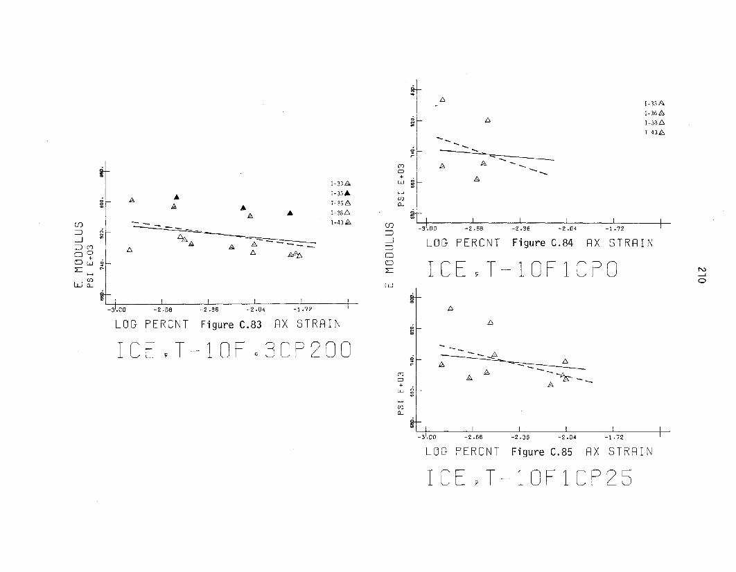
'"..[::,
1-33&
1-368
~I[::, 1-386
1-43b..... ..... ..... .....
¥l- .::::
b.....
b .....gr -- --
1-33& w ~&
A 1-35'" ~
~IR, (J)
R, A1-368 0-
R, A 1-386 :;;CD -- 1-43b CD- ---:::J a :::J..
[::,8-J '" 8---- __ -J LOG PERCNT Figure C.84 RX STRRIN:::J(l1 So .& :::J[::,0° [::,
~ 0(:) + .w ~ (:) ICE 9T-1OF1CPO::L r- ::L N~ .......
wg: 0w
'" '"'" '"
.1[::,
LOG PERCNT Figure C.83 RX STRRIN [::,a~
ICE 9T-1OF a3CP200~'1
- ---- ~b - [::,
--b-~-.&8 -
w ~
~
(J)
CL
LOG PERCNT Figure C.85 RX STRR I N
ICE9T-10F1CP25

N--'--'
1-33&1-3681-386
1-43AA
&&-~&6-
LOG PERCNT Figure C.88 RX STRR I N
ICE9T-IOFICP200
'"'" IA
(J) gl Q
::J '"~
~~- -
::J ~0 . --0 6 &
::c (l1
0
w ~ ~r-
~
(J)
a...
~
6 :--'3&;-368
~rA 6 :-3~6
- 8:-~3 A- ---
~-----&
;\ A
& A(l1
0... .w :~
(f)
a...
~(J)
=:)
~ LOG PERCNT Figure C.86 RX STRRIN::J00 ICE9T-IOFICP50::c
w0.'"'"
J A A"i'>......
....... ...... ....... --
~'[~
-~ ..............6....... 8
w 0........~
r-.......
~
(f)
a...
~! I ! !
-3.00 -2.68 -2.
LOG PERCNT Figure C.8? RX STRRIN
ICE 9T-IOFICPIOO

"'I :g
1-336\ 1-336\
1-368 1-368
~r1-43.;6
.;1-43.;6g
$;
g ~0
...... _-- ......" - i-" -..--tD '"
(Y) (Y) -&_-~0 0+ . + .
2,-- _
w : w ~ --...~
(J) (J)Q... Q...
0c
on ll:UJ (J)
=:J =:J-.J LOG PERCNT Figure C.89 RX STRRIN -.J LOG PERCNT Figure C.91 RX STRRIN=:J =:J0 00 ICE 9T-IOF5CPO 0 ICE 9T-IOF5CP50::L ::L
N~
waI
wI
N
.,'"
~r- 0
'"'"
2,
~.; --...g s..- _
(Y) b (Y) - A .......................0 A 0 -+ . ;;:----- --- .........+ . :8 --"""---w ~ - - w 0
" - --'" -- b~
6\ -- - ~
~--(J) (J) --Q... Q... 2,
"' ~"' I I I I-2.36 -2.04 -1.72
LOG PERCNT Pigure C.90 RX STRRIN LOG PERCNT Figure C.92 RX STRRIN
ICE 9T-IOF5CP25 ICE 9T-IOF5CPIOO

213
«1<l~M co M
~ '( '7 Z0
0:::et:: 0C-J
r: f-,. (f) N«1 x 0-
0:::
... Uc: (V') LD
~C-J 0'>I 0
u LL«1
OJ0~
(0 ::s'? en
~C-J
or-I l..L-
If- r-z
~ <XJ Uu:; et:: Ch
C-JI W
W(L
0 Ua 0c: -l f-----lC")
I
20+3 ISd
SnlnOOW :3

~
oN
LOG PERCNT Figure C.94 RX STRRIN
ICE9T-IFc3CPO
-2.76 -2.44 -2.12 I
~
N.......&
- --- &D" -- -- -.. A---f:,
1-54 A
I-55L'.
1-56&
-----~ A--... B
'"'"
(j)~
::::J--l::::J0 @0LcrJ
0+
lLJw~
-if)CL
...IL ---"-- ---4I11III"
-=----------
Ii, I II I
I-54 ...
I-55 L'.i-56 A
.6
- -... f:,
---
0
'"crJ0+w 0
'"N-if)CL
w
(j)
::::J--l::::JooL
'"'"
00
'"
0N.
crJ0+
W 0
'"-if)CL
- ..... _B_... ...-- -.. "8----/\
lS----':
& - ..
LOG PERCNT Figure C.96 RX STRRIN
ICE9T-IFc3CP50
LOG PERCNT Figure C.95 RX STRR IN
ICE9T-IFc3CP25

LOG PERCNT Figure C.97 RX STRRIN
LOG PERCNT Figure C.99 RX STRRIN
U'1
N
&
I-54 itt.
I-556
[-568
4--..fi:, ~
L::,
~---L::,
&--~-
ICE9T-IFICP50
~
~
0.0.
(f) ~
::J-!::J 0.
N0O(Y)
2::0..0.WW '"
~
(J)
a...
1-544
1-556
1-568
--~& -
-L::,- -- - t
-- < ..L::,
&
&
4
&
----
4 L::,
- ....
*A'-- _------- ----
ICE9T-IFICPO
0.~
0.N
~
(Y)
0..W ~
~
(J)
a...0.~
(f)
::J-!::J002::
W
0.~
~
0.0.~
0.N
(Y)
0..W ~
~
(J)
a...
LOG PERCNT Figure C.98 RX STRR I N
ICE9T-IFICP25

ICE9T-IF5CPOFigure C. 100 RX STRRI N
'"N
'".M(YJ
o...w ~
CDUJ(L
:::J---l:::JooL
w
LOG PERCNT
•£:,
8
•
I-54.
1-55.6
1-568
"w
UJ ~:::J---l:::J 0
'"0 .O(YJ
LO...w S'W '"~
CD(L
..~-- .--__ - __ A
L:s. ------------L!!F-.. --
I-54.
1-55.6
1-568
•8
N--'
'".,'"
'"'"'"
~:l- - •- -f:>.._ •
:z;<; =- - - -~
Ii>
CD(L
Q
'"N
LOG PER CNT Fi gure C. 101 RX STRRIN
ICE9T-IF5CP25
LOG PERCNT Figure C.102 RX STRR I N
ICE9T-IF5CP50

---------
'"~
oo~
~
(Y)
o+w ';
~
(f)
0...
1:::,
•
1:::,
••
1:::,
I-50 A
I-51 •
~
o
'"~
oo
(Y)
o+w ~
(f)
0...
b,
A
f:::,
A
I-50.
I-51 A
A
A------1:::,
1:::,
(f)
=:J--.J=:JooL
w
'"~
'"~
LOG PERCNT Figure C.l03 RX STRR I N
ICE9T-4Fa3CPO
(f)
=:J---.l=:JooL
w
LOG PERCNT Figure C.l05 RX STRRIN
ICE9T-4Fa3CP50'"'"
N--'""-J
1:::,
--------A
-== - ---is L. 1:::, 1:::,
oo
o~
(Y)
o+w ';
~
(f)
0...
1:::,
• A
•- -1:::,--- _ _ •--
1:::,
o'"~
oo~
(Y)
o+w ~
(f)
0...
A
------ • •
LOG PERCNT Figure C.l04 RX STRRIN
ICE9T-4Fa3CP25
;';
LOG PERCNT Figure C.l06 RX STRR IN
ICE9T-4Fa3CPIOO

<Du>
I-50'"
I-51 A
::lI-50 ...
I-51 A
oou>
o..b.
b. b.
------
...b.------
b.
...b.
......ofi:
(Y)
o+w 0
N
b.
A.
------A.
----A.
~
(Y)
o+w 0..,
enCL
enCL
(JJ
~
-..J~
ooL:
W
<DN
LOG PER CNT Fi gure C. 107 RX STRRI N
ICE9T-4FICPO
(JJ
~
-..J~
ooL:
w
;;
LOG PERCNT Figure C.109 RX STRR I N
ICE9T-4FICP50 N-'(Xl
<D<D '"'"
o..u>
o:g
b.
b.
~ I I I! I
oo~
(Y)
o+w ~
enCL
~
... -----...
b.b.
- - - -A.- - ~
...
og
(Y)
o+w ~
enCL
b.b. 6-
... A ... ...
LOG PERCNT Figure C.10B RX STRRIN LOG PERCNT Figure C.110 RX STRRIN
ICE9T-4FICP25 ICE 9T-4FICPIOO

LOG PERCNT Figure C.l11 RX STRRIN
ICE9T-4F5CPO
..
1''::>--''.Q
A
i-50£
I-51 L::.
--- - -~ - 6 6.. -- -
LOG PER CNT Figure C. 11 3 RX S TRRI N
ICE9T-4F5CP50w
J-~I
~~~~
(Y) ,
~ ~~
:i' ~b I I I I I(f) -3.40 -3.0B -2.76 -2.44 -2.12=:J--.J=:Joo:L
[-:)0"
[-0, I L::.
............ ......
......
6
...... ...... ......
............
,,6
......
......
o
'"
~
(f)
CL
~
"'
~
t
(Y")
o+w 0
'"
w
U)
=:J--.J=:Joo:L
o~
'"
oo'"
--- ~-... L::.- -(Y")
o+w ~
L::...(f)
CL
~
'"
LOG PER CNT Fi gure C. 112 RX S TRRIN LOG PER CNT Figure C. 11 4 RX S TRRI N
ICE9T-4F5CP25 ICE9T-4F5CPIOO

iZl ~:-'>A: '>; L:,
~r- 1--~
1-02 ~ --- -A..L:>-_• 1\
I-S3L:, ---0
- -LA_ --~0 - --.,1\- _ 0
"' -4.- "'(Y) 6- ____
(Y)
0 0... . ... .w ~ UJ ~
~ ~
CD (f)
Q... Q.... c.'" '"
(f) (f)
:::J :::J
-1 LOG PERCNT Fi gure C.115 RX STRRIN -1 LOG PER CNT Fi gure C. 117 RX STRRIN:::J :::J
0 0
0 ICE 9T-10F o3CPO 0 ICE9T-1OFa3CP50L L NN
W0
w
! g"'
i~ - - -AJ:"- - - -.4.-.6.- ..
- -~---_A-z:::,. ---J?-
0 1\- ... ..
-~--0
g 0
--:il',. "'(Y) (Y)
0 0... . ... .W 0 W 0
N N
~ ~
(f) (f)
Q... Q.... '<
'" "" I-2.12
LOG PERCNT Figure C.116 RX STRRIN LOG PERCNT Fig ure C. 118 RX STRRI N
ICE 9 T-10F o3CP25 ICE 9 T-10F a3CP1OO

~-
:-52 A
I-53~
---~~
---.... - - -A-L'>... .... ~_n_
- - - ~- - - -,A-.L'>_ A.
"'w
om
'"
0m"'
00
'"(Y)
0+w ~
~
(f)
Q...
--- ~.1
0
'"'"(Y)
0+ .w §~
(J)
Q...
;(j)
=:J--.J LOG PERCNT Figure C.121 RX STRRIN=:J00 ICE9T-IOFICP50L:
NN
W
0.WW
- - - ~ - - - J-I\ _ ..
-,.
___ ...,.... I-52A
--- ..-f':, I-53~
--- - - •. --Dt-_
---~-
ICE9T-IOFICPOLOG PERCNT Figure C.119 RX STRRIN
"'"'
0m
00
'"(Y)
0+w ~
~
(f)
Q...
'"'"
(j)
=:J--.J=:J00L:
W
:g
0m
'"
00
'"(Y)
0+
w 0N~
~
(f)
Q...
0.
'"
LOG PER CNT Figure C. 120 RX STRRI N LOG PERCNT Figure C.122 RX STRRIN
ICE 9T-IOFICP25 ICE 9 T-IOFICPIOO

J;.
- I~52'"
~ :~: - oS? Ii.-- .... - -fr-_ ...... I~53 A - .. - .. :~53A
-es- _ l::::. - - ... c:LC--0 -0 - -'" - --,6,_
(Y] L::.0 0+ . +
W ~ W ~
~ ~
en en(L (L
~(f) -3 1.40 -3.08 -2.76 -2.44 -2.12 I (f)
~ ~
.--J LOG PERCNT Figure C. 123 RX STRRI N .--J LOG PER CNT Figure C. 125 RX STRRI N~ ~
0 00 ICE9T-IOF5CPO 0 ICE9T-IOF5CP50L L N
NW W N
1 <;....
-- - _A_ fE
K --~"'
==tS__
I - - - -"-.6-- •- E - ~-- ... -
~l0
"'"'(Y)
0+
w ~ w 00
'"~
~~(f)
(L
0.
'")40
I I I I I ! I !
-3.08 -2.76 -2.44 -2.12 -3.40 -3.08 -2
LOG PERCNT Figure C.124 RX STRR I N LOG PERCNT Figure C.126 RX STRR I N
ICE9T-IOF5CP25 ICE 9T-IOF5CPIOO

APPENDIX 0
CYCLIC TRIAXIAL TEST RESULTS:DAMPING RATIO OF ICE
Figures 0.1 to 0.19 show test results of damping ratio for highdensity ice, and results for low density ice are shown in Figures0.20 to 0.28. The dashed lines in the figures represent the leastsquares best fit line of the data for a given test condition. Thesolid lines represent the average least squares best fit line for allthe experimental data drawn through the "center" of the data set fora given test condition. (Refer to Section 4.5.1 and Figures 4.63 and4.64 for further explanation.)
223

«l<J~224
0"''''"" "" "" z, , ,- - - CL~
\ ITn:::: U\ f-
.... .... \ 0 ([) --.J\
~<I <I ... x --.JI
\ IT\ IT
<I ......... \ (I)~ <I <I~<iJ N
\ 0Cl 0
"'! OJ\ N S- LLI:::Jen
\ .....~l..l-
\I\
.... ~<I .... <I \<1 <B:::J<iJ~ 0
f-t-<J:<l a; Z
\ N UI '"\ n::::
w\ 0- W
.... ........ .... <1 <1\ <I <I <I <iJ<iJ
U.... \ <iJ <iJ <iJ 00 0~ -.-J f--l
'"I"6
OIlt::JtJ dWt::JO
<iJ<J .... D-o en '""" "" "", , , Z- - - U~, IT, n:::: --.J, f-
.... .... <@ , 0 ([) --.J~\ <I <J ... x IT\I
IT, LD\
............ ....,~ <iJ<J <J <I <iJ <iJ r- 0
"CI
00\ "'! OJ
\ N S- LLI :::J\ en
\ .....~
\l..l-
\ I........ ..... <J \
~ ~ <J <iJ f-0 t-\ a; Z, N UI n:::: '"\
\ WW0-
0 U0 0~ -.-J f--l(T)
I
• L
OIlt::JtJ dWt::JO

1-40.A
1-45A
1-49&
f:;.
46~
.&
f:;.
NN
.&
.&
c.n
£:,8
.& .&
----~f:;. ~ •
f:;. 8
i~
£:,
£:,
£:,
o• t I I I I I
oJ
WoooOJ
NoI
Wooo
LD
No
IWooo
e-
I--l
No
IWooo
o ,;,
I-0::: N
o0::: ~
oo
0- c;L: 0:::o
1-408
1-45 L.1-49.&
..
.&
.&
f:;.
1
-~f:;.
f:;.M8£:,
o• I I I I
0I
W00c;OJ
C'J0
IW000
e-
C'J0I
W00c;lJ)
C'J0
IW00
0c;(Y)
I--l
I-0::: C'J
00::: J
w00
0- c;L: ~
0:::0
-3'.00 -2.60 -2.20 -1.80 -3'.00 -2.60 -2.20 -1.80
ICE 9 T-IFIRLLCP ICE9T-IF5RLLCPLOG PERCNT Figure 0.3 RX STRRIN LOG PERCNT Figure 0.4 RX STRRIN

226~<:]<Q..a<lL!) l..O ...... <:j" r---M M o;:j" o::::t «::j
ZI • I I ,
.................... - - - 0-I--<
IT0:: UI-
<I <I <:] <Q<Q • a (J) ----la;- x ----lI
a:IT
~ ~I.D (I).
I ~"'I ~ ~ Cla c
I "': OJ
""s..
LLI ~0)......
NL1..
II
J~~"'I ~I
"'I ~<I <% ~ a l-f-<:] ~ • a; Z
"" UI I 0-0::I W
W~ ~
G.-
<I <I <I <I~~<:8 0 U
I <QC) (:)
~~ ---..J f------I
'"Io·
OIltltJ dWtlO
<Q ..a <l CL~ <t r-<t <t <t Z, , ,~ ~ ~
I--< Ua:\ 0:: ----l\ I-
<I <I <Q a (J) ----l~"'I
\ a;\ I x IT\ a:\ UJ
<1<1 <I \ ~~~ ~ L!') 0Cl
ca\ "': OJ
\ "" s.. LLI~
\0)......
N\L1..
\ I"'I ~~"'I "'I I-a f-~ ~ a; z\
"" UI
0:: '"\\ w
W\G.-
O Ua (:)
~ ---..J f------I
'"I. s
OIltltJ dWCJO

NN......
fla
.&
-1.80
i
-2.20
1-368
1-418
1-44&
1-47 b.
8.6.
i
4. ~~ ~i ft__~,. M &>b. ~&> &>~ it>
21'.M>.
-2.60
A
-3'.00
a• I I I I I I
C'J0
IW00
~en
N0
IW00
~['
N0
IW00
c:lD
N0
IW0ac:
0 l'"l
I----<
f-a: N
a0:::: I
W00
0.- c:L: -IT0
-1.80-2.20-2.60
1-368
1-418
1-44&
1-47 I::>
& I::>
it>
I::>
1::>&it>
~
~I::>.&
~ 8
il::>~
I::>~
A _--
~
.-.-, -.-
_A- -- -- --~
.&
~ Wit>
8
~
~
it>~t
it>
it>it>
.&
-3'.00
o• I I I I I I
0I
W00
~en
C\l0I
W00
~['
C\l0
IW00
~lD
C\l0
IW00
~0 C')
I----<
f-a: C\l
00:::: I
W00
0.- ~L: ~
a:0
ICE9T-2FIRLLCP ICE9T-2F5RLLCPLOG PERCNT Figure 0.7 RX STRRIN LOG PERCNT Figure 0.8 RX STRRIN

~«]«I<J<Sl228
U)\ONl.OCOM M '<:j" 'd" o::::t ZI I I I I...........................................
CL.........
I a:1 0::: U
I-
~ ~ <J <J «]1 ~ 0 (J) ---.--J1<tJ
<llII ~- ---.--JI Xa:
I IT~~ <J <J ./~<tJ <llII
a(I)r-
0
<llII <J 0, 0 0
Ic-; OJN S0-
Li-I :JC)
Or-
~l.J..II I
~ <1J <41 ~~ I~
I-~
0
1 <llII<llII U; ZN U
I I0::: '"
I wWI CL
<l<J~ ~~ <tJ 0 U
I 0 0c:; -J I--l
""Io·
OIltJ~ dWtJO
<tJ<J CLN "'~ "1 Z
......... U\ a:
\ 0::: ---.--JI-
\ 0 (J) ---.--J<J~
~- X ITI
\a:
\Lf)
~ <tJ <l<tJ<tJ 0) 00
00
~ c-; OJN S0- Li-\ I :J
\C)
Or-
~l.J..\
\ Iq:J <J<J <tJ \ <tJ<J «I<tJ 0
I-~\ U; Z
N U\ I
0::: '"\ W
W\ CL
0 U0 0c:; -J I--l
""I° s
OIltJtl dWtJO

1-368
1-42&
1-466
1-48,0,!~1-368 0
I
1-42 A.w00
1-466 C?1-488
0)
N N0 0I I
W W0 00 0
C? C?r-- r--
N N0 0
I IW W0 00 12:. 0
~ C?lJ) to
~~ 12:.
,0, ~ tN 12:. N0 12:. ItJ 12:.
0I M I
W 6 w0 D. 00 & 00 ------ 0--7'--- - -0 C'l 0 C'l
.......... ) & ..........f- &8 f-a: N a: N
0 As. 0et::: I 8 et::: I
W W0 00 0
(L ~ (L ~L: .... L: ....a: a:0 0
~
~&
---.88
fK~
---&~
~
""
~-- -.~--A A& B
NNl.O
o• I I ! ! I I
-3'.00 -2.60 -2.20 -1.80
C?-3'.00 -2.60 -2.20 -1.80
I
LOG PERCNT Figure 0.11 RX STRAIN LOG PERCNT Figure 0.12 RX STRRIN
ICE9T-4FIRLLCP ICE9T-4F5RLLCP

<:1<1 230'"' OJM M
Z, I
1-----4
I a:I 0::: 0--.
«:) 1«:)f-
<1<l C> (J) UI ~- x .--JI I
a:1 .--J,
.q- IT<l,~«:) ...--.I C> Cl
~
I"': OJINI s.. LL::s
CJ)
CO1 .....LL..
1 I1<1<1~, ~«:) C>
f-f---~ z
1 IN UI
'"I 0:::W
I (L W<l:::1 <1<1 I <1 0 UI
C> <'::]c; -..J I-----l
'"I
OIltJ~ dWtJO
.<:1<1en '"' co ZM M M
I I I
0--.1-----4
a:I
0::: Uf-
~«:) 1«:) C> (J) .--J1 ~ ~
7 x .--JI a:I IT
~., I (Y) (I)~«:) ...~ .
C> Cl c
I "': OJI IN s.. LLI
::sI CJ)
CO.....LL.., I
<]::J <l <l <l ~. ~ C>f-
f---I ~ ~~ ~ ZIN U
I I
'"0:::I WI (L W
<1<1 <1<l~ 0 U,C> <'::]c; -..J I-----l
'"IO'
OIltJ~ dWlJO

231 CL~ Utv)
Z.".,-l>----<
IT0::: -l\ f---
\ 0 (fJ IT<lJ~
0::7 x LD\ IT
\ 0\
~ a<lJ
0 Cl LL"'!\ '"
Q)
0\I ~
:::5
\ 01'r- ~
\ lL.
\ I
~0
f---f---U; z
'" U\
I Q,.Q:::
\ WlLJ(L
Q U0 0~ -.J 1-----1
'"I• 8
OI1CJtJ dWCJO
<iJ'.<:Jtv) Z,
>----<
/ IT
/ 0::: 0-<iJ«f
f---0 (fJ U
/ 0::
/ 7 x -l/
IT-l
// <iJ
U') IT.«]0 Cl LD"'!
/ '"Q)
I ~ LL/ :::501
/ 'r- eolL./ I/
/<iJ 0f---
f---<iJ <iJ/ «] U; Z
'" U/ I
0:::Q,.
/ wlLJ(L
Q U0 0c::; -.J 1-----1
'"I0'
OI1CJtJ dWlJO

1-368
1-3S!:;,.
1-43~
L'::.L'::. L'::. !:;,.
!:;,.L6 ~ i}
__ I!;, - --.----IC:.J!,.: if,
J!,. ~J!,. t J!,.
0I
W00
~en
'"0IW00
~e-
'"0I
W00
~ID
'"0I
w00
~0 cry
1---4
I-a:: '"00::::: I
W00
(L ~L: ~
a::0
L'::. L'::. ~L'::. L'::. L'::.
L'::. L'::.L'::. L'::. L'::.L'::. L'::.
8 ~ 88 -~ _ ' __ ..8- --- - - - ¥- - - . IE
-t--" J!,. 8 AJ!,.~J!,. &, J!J,;A A
J!,. ~ ~.
J!,.
~A
1-35.N0
I
1-368 w0
1-3S!:;,.0
~1-43~ en
'"0I
W00
~e-
'"0I
W00
~IJ)
'"0I
W00
0~cry
1---4
I-a:: '"0:::::
0I
W0
(L0
~L: ~
a::0
J!,.A
-1.80-2.20-2.60-3'.00
o• I I I I I I
-1.80-2.20-2.60-3'.00
LOG PERCNT Figure 0.17 RX STRRIN LOG PERCNT Figure 0.18 RX STRRIN
ICE9T-IOFo3RLLC ICE9T-IOFIRLLCP

233
<::J~<D M
M '" Z, ,I---l CLIT0:: UI--
~ 0 (f) ---l~
<ll - x ---lI
ITIT
0) LD~ <ll r-.
0 Cl LL"!'"
(l)
I S- O::JOl
or-~
I..L..
I«J «J 0
I--f-«J «J <ll u:: Z
'" UI
""0::W
W0....
D U0 <::)
~ -l 1-----1(T)
I
o·
OIlcH:l dWlJO

~a...
I-54. Ii:> 1-544.
1-55.6- 1-55.6-
~~ 1-56.6. N 1-56.6.a
I 1;;.Ii:>
w Ii:>a
~f-a
Ii:> c: 1;;.OJ
1;;.1;;.
N
il 1;;. 1;;. a1
wagl 1;;..r--
1;;.
!~N £ i• a -- =I
Ii:> __~ w t Na 1;;. W
--7»\- a -r:>o
- .... - c: ~A----- LD ..
• £•I •o ~ !1;;. Ii:> 0N £1;;.a
I A ..-.... I •..-.... w wf- g I-
aa
IT c: Il:P a:: c:n:::: CD £ n:::: M
1
£ ;1;
0- N Ii:> 0- NL: a L: 0
1 IIT W IT W
0 0
0 0 0 0
....-3.40 -3.00 -2.60 -2.20 -31. 40 -3.00 -2.60 -2.20
LOG PERCNT Figure 0.20 RX STRRIN LOG PERCNT Figure 0.21 RX STRRIN
ICE 9T-IF o3RLLCP ICE 9T-IFIRLLCP

a....~,
I-54.
~II-50.
[-55.6. 1-51.6.A 1-568
aa
~I 0)I.....
aa
~I Na AIWa Aa A
i~c: Ar--
•.6. N • A ~a A
I A Aw Aa.6. a - -
;~c: A _---UJ - - LS----- .6. AN- - - [:, .6.·w- -- ()1--- A N
- --.--- al\'l J-- - w
aA -- ......
~ :, f!j ~
o ?~ ;. .6.O--l w
A .6.I- g .6.
.6.
a: c:~
IT N
0:::: C'"J0
0:::: IW00
il- u 0- c::L: 0 :L: ~ I .6.Ja: w IT0o a 0
c5• I I I I I
-3'.40 -3.00 -2.60 -2.20 I -3.40 -3.00 -2.60 -2.20
LOG PERCNT Figure D.22 AX STRAIN LOG PERCNT Figure D.23 AX STRAIN
ICE 9T-IF5RLLCP ICE 9T-4F o3RLLCP

236-c<l .. \~o ~
~ ~'" '" -;>", ,"'-
\ .........
\ IT~ 0-..\ f-
\ 0 (f) U<"!IN X -.-J~I
~ ~ IT~
~~ \-.-J
L!) IT~ \ N
\.
C) Cl UJ\ ~ <J<J ":IN OJ
\ I r... LL::l
\ en~.....
\ l.L.
IC)
f-f-~ z
(r) UI C'-~
WWa....
C) U0 <:)
": -.I f-----.l(r)
I
O'
OIltJ~ dWtJO
~<l~ .. \~o ~
'" '" z, ,\ .........
\ IT~ 0-..\ f-
\ C) (f) U<"!
\ IN X -.-J~ ~~
I
\ IT~~ -.-J... \
\o::::t ITN
C) Cl ~
\ ~ ~ <k) ":OJIN
LLI r...\ ::l
en\ ..... ~.. \~
l.L.
\ I\ C)
f-f-~ Z
\~~<1l '" u
I C'-~ \ ~.. w
Wa....\ C) U
~C) <:)
": -.I f-----.l(r)
I
o·
OIltJ~ dWtJO

f-a:: N
o0::::: J
Woo
0..... 0
:L a::o
I-52.A.
1-536
NW'-!
A.A b. ~... A .& _b. ~
~-- ~ = ~
--, -i~ • b.
0J
W000
en
N0
JW000
e-
N0
JW000
lD
N0
JW000
'" .AI---'
o.& .& .&b. .A
.& D. .itD. ~
b._ - - I/).
A:'__ _ l>-Z- £:"b.
.AD. • .&b.
b. .&
1-52.&
1-536
0J
W000
en
N0
JW000
r0-
N0
JW000
lD
N0
JW00
~0 (f)
I---'
f-a: N
00::::: J
W·00
0..... ~:L -a:0
o• I ! [
o• I I I I I
-3'.40 -3.00 -2.60 -2.20 -3'.40 -3.00 -2.60 -2.20
LOG PERCNT Figure D.26 RX STRR I N LOG PERCNT Figure D.27 RX STRRIN
ICE9T-10FD3RLLCP ICE9T-10F1RLLCP

238
~<l
~ <JN M <llII ZU) U)
I I
~\I---<
ITI et::: U\ I--
0 UJ ~<J<J <J <J "'!<llII. <llII<llII
N x ~I
IT\ IT\ co LD\<J<] N
~ I<J 0 Cl LL\~ u:;N OJ
0I I s..::::l
\ en.....~
I l..L..
I I\ 0
I--f-
IC; zen U
I
'"et:::W
W0-
0 U0 <:)
"'; --.J t--lenI
O'
OI1[J~ dW[JD

APPENDIX E
CYCLIC TRIAXIAL TEST RESULTS: DYNAMICYOUNG'S MODULUS OF FROZEN CLAY
239

00Ol
00CO
00t-
en:::) 0
-.J 0CD
:::)
0<::) 0
0L: LD
W00....
0
(Y) 0C'l
0+
W00N
I-----l
(j) 00
CL
c5
SAMPLES CL-l,CL-2ALL CONFINING PRESSURES
WATER CONTENT =29.2%30 POINTS
00Ol
00co
00t-
(j)
:::J 0
--.J 0CD
:::J0c::J 0
0:L: LD
W00....
0
(Y) 0C'l
0+w 0
aN
I-----l
(j) 0._a
CL
c5
SAMPLES CL-l,CL-2Ali CONFINING PRESSURESWATER CONTENT=29.2%
30 POINTS
N~o
LOG PERCNT Figure E.1 RX STRRIN LOG PERCNT Figure E.2 RX STRRIN
O-CLRYT-l~3 O-CLRYT-IFl

SAf1PLES CL-l,CL-2ALe CONFINING PRESSURES
~r WATER CONTENT=29.2~00m
30 POINTS
0 00 0OJ OJ
0 00 0r- r-
UJ UJ=:J 0 =:J 0
-.J 0 -.J 0ill ill
=:J =:J0 00 0 0 0
0 0
L lJ) L lJ)
W W0 00 0... ...
0 0
CD 0 CD 0(r) T)
0 0+ +
W0
W0
0 0N N
>---< >---<
en 0 uJ 00 0
CL - CL -
SAMPLES CL-2,CL-4ALL CONFINING PRESSURES
WATER CONTENT=29.2%
28 POINTS
N.t:>..-l
Fi gure E. 4LOG PERCNT
o. I I I I I I I f--
.0
RX STRRIN
I I-.500 .01
RX STRRINFi gure E. 3LOG PERCNT
o
O-CLRYT-IF5 O-Cl_RYT 4 Fo3

N~N
SAMPLES CL-2,Cl-4ALL CONFINING PRESSURES
WATER CONTENT=29.2%
28 POINTS
RX STRRIN
a
-1.50
Figure E.6
i~
LOG PERCNT
C?I I I [ I I ! -:at-
0aOJ
00co
0co<-
en:::J 0
--.J 0CD
:::J00 0
coL: Lf.l
W00....
0
(Y) 0(Y)
0+
0w 0N
I---l
(j) 00
CL
SN~PlES Cl-2,CL-4All CONFINING PRESSURES
WATER CONTENT=29.2%
28 POINTS
RX STRRINFigure E.5LOG PERCNT
0.:0C1l
00CO
00<-
en:::J a
0--.J (D
:::J0
a0 0L: Lf.l
W00....
0co(Y) (Y)
0+ co
W coN
I---l
(f) 00
(L
0
O-CLRYT-4Fl O--CLRYT -4F5

~ gL0.- -I
~tl I I I I , I-3.00 -2.50 -2.00 -1.50 -1.00 -.500 .0
UJ::J--.I::JooL
W
ooOJ
ooro
CJCJr-
ooCD
ooLD
oo..,.
o(Y) 0
cr>
o+w g
N
SAMPLES CL-2,CL-3ALL CONFINING PRESSURESWATER CONTENT=29.2%
29 POINTS
00OJ
00ro
UJ :[ ~::J--.I
0(D
::J00 0
0
L CD
W00..,.
0
(Y) 0cr>
0j-
w 00N
~
UJ 00
0.- -
-2.00
SAMPLES CL-2,CL-3AIL CONFINING PRESSURESWATER CONTENT=29.2'
27 POINTS
N-::::.w
LOG PERCNT Figure E.7 RX STRRIN LOG PERCNT Figure E.8 RX 5 TRRI iJ
D-CLRYT'-l O~3 O-CLRYT-IOFI

a. I I I I I I I
-1.50 -1.00 -.500---~--
aaOJ
a ~_
aro
aae-
(fJ
:=J a--l
aCD
:=J00 0
aL LJ)
WC0-GV
0
(T) 0(T)
0+
WCo-.0(J
>---<
(f) 0
0-Co-
c
SAMPLES CL-2,CL-JALL CONFINING PRESSURESWATER CONTENT~29.2%
aaen
27 POINTS
0aro
aae-
(fJ
:=J 0
--l aCD
:=J00 0
aL LJ)
W0av
a(T) a
'"0+ gl--W
£::,
C"
>---<
(J) 00
0-
SAMPLES C-30-2,C-30-4ALL CONFINI,iG PRESSURESWATER CONTENT=36',
39 POINTS
i"V-Po.;.:,.
LOG PERC NT Figure E.9 RX STRRIN LOG PERCNT Figure E.10 RX STRRIN
O-CLRYT-1DF5 O-CLRYT -1 FaD5

N+>0CJ1
SN~PLES C-30-2,C-30-4,C-5-2ALL CONFINING PRESSURES
WATER CONTENT=36%
53 POINTS
o• I I I I I ! I I
000)
00co
00('-
(j)
=:) 00
---I CD
=:)
000 0
L: lJJ
W00...
0
(Y) 0('1
0+
0w 0N
.........(f) 0
0CL
SAMPLES C-30-2,C-30-4,C-5-2ALL CONFINING PRESSURES
WATER CONTENT=36;:
54 POINTS
000)
00CD
00('-
(j)
=:) 0
---I 0CD
=:)
00 0
0L: If)
W00...
0
(Y) 0
""0+w 0
0
'">---<
(f) 00
CL -0
LOG PERCNT Fi gure E. 11 RX STRRIN LOG PERCNT Figure L12 RX STRRIN
O-CLRYT -1 Fc3 O-CLRYT-IFl

00
'"00ex>
00r--
(J)
:::J 0
-l0CD
:::J00 0
0
L: lJ:)
W00...
0
(Y) 0(Y)
0+w 0
0N
f--l
(f) 00
0-
0
SAMPLES C-30-2,C-30-4,C-5-2ALL CONFINING PRESSURESWATER CONTENT;36%
54 POINTS
00
'"00ex>
00r--
(J)
:::J 00
-l CD
:::J0
00 0
L: lJ:)
W00...
0
(Y) 0(Y)
0+
0w 0N
f--l
(f) 00
0-
o
SAMPLES C-30-1,C-30-5,C-5-1
ALL CO"FINING PRESSURESWATER CONTENT;36%
53 POINTS
N~O'l
LOG PERCNT Figure E.13 RX STRRIN LOG PERCNT Figure E.14 RX STRRIN
O-CLRYT-IF5 O-CLRYT -4Fc05

N,J:::>'-J
RX STRRIN
SAMPLES C-30-1,C-30-5,C-5-1,C-5-2ALL CONFINING PRESSURESWATER CONTENT=36%
68 POINTS
Figure E.16
I I-2.00
LOG PERCNT
o• I I
00(J)
00CD
00e--
00CD
00UJ
00....
0
(Y) 0('")
0+w 0
0C'J
f----l
(J) 00
CL
w
(J)
:=J-I:=JooL
RX STRRIN
SAMPLES C-30-1,C-30-5,C-5-1,C-5-2ALL CONFINING PRESSURESWATER CONTENT~36%
68 POINTS
Figure E.15LOG PERCNT
00(J)
00CD
00e--
(J)
:=J 0
-I 0CD
:=J00 0
L0UJ
w J ~0....
0
(Y) 0('")
0+
W00C'J
f----l
(J) 0
CL0
0
O-CLRYT -4Fo3 O-CLRYT-4Fl

SM~PLES C-30-1,C-30-5,C-5-1,C-5-2
ALL CONFIN'NG PRESSURES
~r WATER CONTENT=36~000)
68 POINTS
0 00 0a::> a::>
0 00 0r- r-
(J) (J)=:) 0 =:) 0
-l 0 -l 0CD CD
=:) =:)
0 00 0 0 0
0 0L: If) L: If)
W W0 00 0.... ....
0 0
(Y") 0 (Y") 0C"J C"J
0 0+ +
W0
W0
0 0
'" '">---I >---I
UJ 0 UJ 00 0
0- ~ 0-
0 0I I I I I
SAMPLES C-30-3,C-30-6ALL COIjFINI,iG PRESSURES
WATER CONTENT=36~
34 POINTS
N.;:..ex>
LOG PERCNT Fi gure E. 17 AX STRAIN LOG PERCNT Figure E.18 AX STRAIN
O-CLRYT-4F5 O-CLRYT-I0~05

N.J:»'-0
SAMPLES C-30-3,C-30-6,C-5-2,C-5-3
ALL CONFINING PRESSURES
WATER CONTENT=36%66 POINTS
SAMPLES C-30-3,C-30-6,C-5-2,C-5-3
ALL CONFINING PRESSURES
~I0
WATER CONTENT=36% 0C)
67 POINTS
~r00lD
~. , ...0 00 0e- e-
(J) (J)
:::J 0 ::J 0
--.J 0 --.J 0CD CD
::J ::J0 00 0 0 0
a 0L: lD L: UJ
W W0 00 0... ....
0 0
(Y) 0 (Y) 0C"l C'?
0 0+ +
Wa
W0
a 0e-J '"
1--1 1--1
UJ a UJ 0a 0
CL - CL
a c:51 I I I I I
LOG PERCNT Figure E.19 RX STRRIN LOG PERCNT Figure E.20 RX STRRIN
O-CLRYT~lO~3 O-CLRYT-IOFl

SAMPLES C-30-3,C-30-6,C-5-2,C-5-3
ALL CONFINING PRESSURES ·~r-
0WATER CONTENT=36% 0
'"66 POINTS
0 00 0(0 (0
0 00 t:Jr- r-
(f) (f)
::) 0 ::) b.....J
0 .....J t:JCD to
::) ::)
0 0 ·(':) 0 (':) 00 t:J
::c If.) ::c LD
W . W0 00 0.... ....
·0 0
(I) 0 (I) t:J(T) (T)
0 0+ +
W0
W0
0 t:J
'" N
>--I >--I
(j) 0 (j) 60 0
(L ..... (L .....
c:: 6
SAMPLE C-30-7ALL CONFINING PRESSURESWATER CONTENT=46.3%
16 POINTS
N(J1
o
LOG PERCNT Figure E,21 RX STRRIN LOG PERCNT Figure E.22 RX STRRIN
O-CLRYT-IOF5 O-CLRYT~1~3

Iill
N()"J--'
SAMPLE C-30-7
ALL CONFINING PRESSURES
WATER CONTENT=46. 3';
16 POINTS
----j-.0
RX STRRIN
~
~
Figure E.24LOG PERCNT
o
000'>
00CD
00r-
(j)
=::) 0
-l 0CD
=::)
00 0
0L: LD
W00....
0
(I) bC')
0+w g
N
I---l
(f) 6b
(L
SAP1PLE C-30-7
ALL CONFINING PRESSURES
WATER CONTENT=46.3
16 POINTS
RX STRRINFigure E.23LOG PERCNT
0b0'>
·0bCD
00r-
(j)
=::) 0-l b
ID=::)
00 0
0L: LD
W00....
·0(I) b
C')
0+ ·0
W 0N
I---l
(f) 00
(L
b
O-CLRYT-IFI O-CLRYT-IF5

NU1N
SAMPLE C-30-7ALL CONFINING PRESSURESWATER CONTENT~46.3~
16 POINTS
AX STRAINFigure E.26LOG PERCNT
o• I I I I I I I I
·00en
b0co
>00r-
CD0=:) 0CD-J
=:)
·00
0 0LnL:.
W 00....
·00CD (')
0+
0w 0C\J
>---<
(f) 00
0....
SAMPLE C-30-7ALL CONFINING PRESSURES
WATER CONTENT~46.3%
16 POINTS
AX STRAINFigure E.25LOG PERCNT
00en
00CO
00r-
CD>
=:) 0
-J 0CD
=:)
00 0
0L:. Ln
W00....
0
CD 0(')
0+w 0
0C\J
>---<
(f) 00
0....
c:5
O-CLRYT-4~3 O"-CLRYT-4Fl
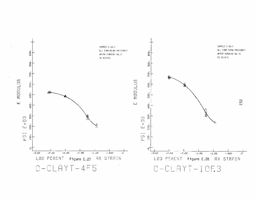
NU1W
SAMPLE C-30-7ALL CONFINING PRESSURES
WATER CONTENT o 46.3%
15 POINTS
RX STRRINFigure E.28LOG PERCNT
o
00en
0010
00r-
(f)
0::J0
~ CD
::J0
00 0illL
W00....
00(T)'"0
+0w 0C'J
I----<
en 00
0-
SAMPLE C-30-7ALL CONFINING PRESSURESWATER CONTENT o 46.3;;
16 POINTS
RX STRRIN
B
Figure E.27LOG PERCNT
000)
0010
00r-
(f)
::J 00
~ CD
::J0
00 0L: LD
W00....
00(T)'"0
+0
W 0C'J
I----<
en 00
0-
0
O-CLRYT-4F5 O-CLRYT-I0~3

N<..n+»
SAMPLE C-30-7ALL CONFTNING PRESSURESWATER CONTENT=46.3%
15 POINTS
RX STRRINFigure E.30LOG PERCNT
o
00O'l
.00(D
00r-
en~ 0
....J0co
~
00 0
0
L In
W00....
0'
0
CD 0C'?
0+w 0
0N
1---4
(f) 00
CL
SAMPLE C-30-7ALL CONFINING PRESSURES
WATER CONTENT=46.3~
15 POINTS
RX STRRINFi gure E. 29LOG PERCNT
00O'l
00CD
00r-
en~ 0
0....J CO
~
0000
L In
W00....
00CD C'?
0+
0W 0
N
1---4
(f) 00
CL
0
O-CLRYT-10Fl O-CLRYT-10F5

NU1(."
SAMPLES CH-3,CH-4ALL CONFINING PRESSURES
WATER CONTENT=55.1
30 POINTS
J I I I.0
o• I I
SAI~PLES CH-3,CH-4ALL CONFINING PRESSURES
0
WATER CONTENT=55.1% 0(J)
30 POINTS
00en
00r-
if.)
:::J 0
......J 0CD
:::J00 0
0L: lJ)
W00....
0
(Y) 0C'"l
0+
W00N
I---< f':,Li (f) 0
CL0
00(J)
00en
00r-
(f)
::::J 0
......J 0CD
::::J00 0
0L: lJ)
W00....
0
(Y) 0O?
0+w 0
0N
I---<
(f) 00
CL -0
LOG PERCNT Figure E.31 RX STRRIN LOG PERCNT Fi gure E. 32 RX S-RRIN
O-CLRYT -1 Fo3 O-CLRYT-IFl

N01
'"
SAMPLES CH-2,CH-3ALL CONFINING PRESSURESWATER CONTENT=55.1%30 POINTS
b
o• I I I I I
00m
0co<D
00r-
(J)
~ 0
.--J 0CD
~
00 0
'ClL lD
W0<::l....
0
(Y) 0(rJ
0+
w 0coC'J
f---<
ef) r:>0
0- -
SAMPLES CH-3,CH-4ALL CONFINING PRESSURESWATER CONTENT=55. L,
30 POINTS
b
b
<::l0m
<::l0<D
o ~_
0r-
(J)
~ <::l
.--J 0CD
=:J0C 0
0L ill
W00....
0
(Y) 0(rJ
0+
W00C'J
f---<
(j) 00
CL
c5
LOG PERCNT Figure E.33 RX STRRIN LOG PEPCNT Figure E.34 RX STRRIN
O-CLRYT-1F5 0-- Cl_ RY T- 4Fo3

c:; I I I I I I I I-3.00 -2.6J -2.00 -1.50 -1.00 -.500 .1
Nc.Jl--...J
SAMPLES CH-2,CH-3
ALL CONFINING PRESSURESwATER CONTENT=55.1%
30 POINTS
~
f::,
000)
00OC)
00r--
([)
::J :::J
--l 0CD
::J00 n
0L l1)
W0:::J
'"
0
:D 0C')
0+w CJ
0N
<--<
(J) 00
0...-
SAMPLES CH-2,CH-3ALL CONFINING PRESSURES
WATER CONTENT=55. 1%
30 POINTS
f::,
f::,
.r00OJ
00OC)
0
"r--([)
::::> 0
--l 0'D
::::>00 0
0
L l1)
W0CJ...
'"(Y) 0
'"0+
W':::)
0N
f---<
(J) 0
0...-0-c:5
LOG PERCNT Figure E.35 RX STRRIN LOG PE.:RCNT Figure E.36 RX STRRIN
O-CLRYT -4F-l O-CLRYT-4F5

SAMPLES CH-1,CH-3ALL CONFINING PRESSURES
gl 0WATER CONTENT;55.1% 0
en28 POINTS
0 ~ 00 0co ill
0 00 0r-- r--
UJ (f)
:=l 0 :=l 0
--.J 0 --.Jco
(IJ (IJ
:=l :=l0 00 0 0 0
0 CJL: LD L: LD
W W0 00 -:0..". ..".
0 0
CD 0 CD 0(')
f:;(')
0 0+ +
W0
W0
0 0N N
1--< <--<
(f) 0 (f) 0a 0
CL. - CL. -0 "?
SAMPLES CH-l,CH-3ALL CONFINING PRESSURES
WATER CONTENT"55.1%28 POINTS
N(Jl
(Xl
f:;
£j.
LOG PERCNT Figure E.3? RX STRRIN LOG PERCNT Figure E.38 RX STRRIN
O-CLRYT -1 OFo3 O-CLRYT-10r-1

SAMPLES CH-I,CH-3ALL CONFINING PRESSURES
~I0
WATER CONTENT~55. 1 0OJ
~ 28 POINTS~
~I ~00ro
CJ 00 0r- r-
(j) CD::J 'C) ::J 0
-l 0 -l 0CD CD
::J ::J0 0<:':) 0 0 0
0 0L LO L LO
W W0 00 0... ...
£::,
0~
0
(Y) 0 £::, (Y) 0C'J (r)
::::J 0+ +
W0 W
0CJ 0;,.'1 N
.......... ..........
'J) 0 (f) 00 0
0..... - 0.....
SAMPLES MC-30-1 ,MC-30-2ALL CONFINING PRESSURESWATER CONTENT~57. 1
30 POINTS
NU11.0
STR8INRXFigure E.40LOG PERCNT
o
RXFi gure E. 39LOG PERCNT
~I"jtlOO-~I;;;----:71:n;;---:f'~_---l.__-L__- I I-.500 .0+-ST~RIN
O-CLRYT-IOF5 OM-CLRYT-l~3

N
'"o
SN~PLES MC-30-1,MC-30-2ALL CONFINING PRESSURESwATER CONTENT=57.130 POINTS
SAMPLES MC-30-1 ,MC-30-2ALL CONFINING PRESSURES
0 I'IATER CONTENT=57. ];"0
0 0C1> OJ
30 POINTS
0 00 0ro ro
0 00 0r- r-
en en::J 0 ::J 0
---l 0 ---l 0co co
::J ::J0 00 0 0 0 ,-
L0 0lJ) L 1J)
W W0 00 0.... ....
0 0
CD 0 CD 0<') '"0 0
+ +W
0W
00 0N (J
......... .........(J) 0 (J) 0
0 00- - 0- ~
0I I I I
0I I I
LOG fERCNT Figure E.41 RX STRRIN LOG fERCNT Fi gure E.42 RX STRRIN
OM-CLRYT-IFl OM-CLRYT-IF5

SAMPLES MC-30-2,MC-30-3ALL CONFINING PRESSURES
0WATER CONTENT=57. 1
00 0m m
30 POINTS
0 00 0co co
0 00 0.... ....
(jJ (jJ
:::J 0 :::J 0
--.J 0 --.J 0CD CD
:::J :::J0 00 0 0 0
0 02: l1) 2: If)
W W0 00 0... ...
0 0
(Y) 0 (Y) 0<'"J '"0 0
+ +W
0W
00 0N N
>--l >--l
(f) 0 (f) 00 0
CL - CL
SAMPLES MC-30-2,MC-30-3
ALL CONFINING PRESSURESWATER CONTENT=57.1
30 POINTS
NO'l--'
o• I I I I L__ ~
··l.OO - .500 .0
o
LOG PERCNT Figure E.43 RX STRRIN LOG PERCNT Figure E.44 RX STRRIN
OM-CLRYT -4Fc3 OM-CLRYT-4Fl

aaCJ)
aaCD
aae--
(f):::) a---l a
CD:::)
00 a
aL l.D
Waa...
a(Y") a
(T)
0+
WaaC'J
1---1
CD aa
(L -0
~
SAMPLES MC-30-2,MC-30-3ALL CONFINING PRESSURESWATER CONTENT=57. 1~30 POINTS
b.
b.
0aCJ)
aaCD
aae--
(f)
:::) a---l a
CD:=J00 a
aL: If.)
Waa....
a(Y") a
(T)
0+
WaaC'J
1---1
CD aa
(L -o
SAMPLES MC-30-2,MC-30-4ALL CONFINING PRESSURESWATER CONTENT=57. 1%28 PCINTS
NO'lN
LOG PERCNT Figure E.45 RX STRRIN LOG PERCNT Figure E.46 RX STRRIN
OM-CLRYT-4F5 OM-CLRYT -1 OFo3

c: I I I I I I I ~_-3.00 -2.50 -2.00 -1.50 -1.00 -.500 .0
ai
SAMPLES MC-30-2,MC-30-4ALL CONFINING PRESSURESWATER CONTENT=57.1%28 POINTS
N0)
w~
R
E!
00
'"00ro
0 <-0r--
(fJ
=:J 0
---l 0CD
::J00 0 ,-
0L: La
W00...
0
(Y) 0crJ
0+w 0
0N
f---l
(J) 00
0..... -
SM~PLES MC-30-2,MC-30-4ALL CONFINING PRESSURES
WATER CONTENT=57.128 POINTS
~
~
~
00
'"
00ro
00r--
(fJ
::J 0
---l 0CD
::J00 0
0L: La
W00.".
0
(Y) 0
'"0+
LLJ00C'J
f---l
(J) 00
(L
0
LOG PERCNT Figure E.47 RX STRRIN LOG PERCNT Figure E.48 RX STRR p~
OM--CLRYT -1 OF 1 OM--CLRYT -1 OF5

APPENDIX F
CYCLIC TRIAXIAL TEST RESULTS: DAMPINGRATIO OF FROZEN CLAY
264

oCl
'"
otn
'"
SAMPLES CL-l, CL-ZALL CONFINING PRESSURES
WATER CONTENT=Z9.Z%
30 POINTS
o
c;
otnN
SAMPLES CL-l, CL-Z
ALL CONFINING PRESSURES
WATER CONTENT=Z9.Z'
30 POINTS
~~ /00
"!
dt; I /
~L0UJ
-:1 /NCTl(J1
I /0 00 S.
0 0I---< '" I---< N
0 0
f- t1., f- IW
0: g 0: g0:::::: c: 0:::::: c;
tn UJ
eL eLL L0: 0:0 0
c: 0• I
-31.00 -2.50 -2.00 -1.50 -1.00 -.500
LOG PERCNT Fi gure F. 1 AX STRAIN LOG PERCNT Figure F.2 RX STRAIN
O-CLRYT-l~3 O-CLRYT-IFl

o
~
o0.(T)
oIJ)
'"
SAMPLES CL-l, CL-2ALL CONFINING PRESSURES
WATER CONTENT=29.2%30 POINTS
oIJ)
'"
SAMPLES CL-2, CL-4ALL CONFINING PRESSURES
WATER CONTENT=29.2%
28 POINTS
oo
'"oo
'"
oIJ)
oIJ)
N
'"'"
RX STRRIN-1.00
Figure F.4LOG PERCNT
00-.
0'">---;0
I--- IW0IT 0
0:::::: ~IJ)
0......L:IT0
0
RX STRRINFigure F.3LOG PERCNT
00-.
0'">---; 0I
I--- w0
IT 0
~0::::: IJ)
0......L:IT0
0
O-CLRYT-IF5 O-CLRYT -4Fo3

oClC'J
ooC'J
oIn
'"
SAMPLES CL-2, CL-4ALL CONFINING PRESSURESWATER CONTENT=29.2~
28 POINTSoIn
'"
SAMPLES CL-2, CL-4ALL CONFINING PRESSURESWATER CONTENT=29.2;.
28 POINTS
oo
'"oo
'"
~L ~0In-• I AJ
NO"'l-....J
I /0 00 0- -.
0 0I---< '" I---< '"0 0
f- ~ f- ~
0::: g 0::: g0:::: c:; £::,. 0:::: c:;
In to
CL CL £::,.L ~ L0::: 0:::0 0
0 0
.! I ! ! I I I
-3.00 -2.50 -2.00 -1.50 -1.00 -.500
LOG PERCNT Figure F.5 RX STRRIN LOG PERCNT Figure F.6 RX STRRIN
O-CLRYT-4Fl O-CLRYT-4F5

<:>aM
<:>InC'J
<:><:>C'J
SAMPLES CL-2, CL-3ALL CONFINING PRESSURESWATER CONTENT;29.2%29 POINTS
<:>aM
<:>In
'"
<:><:>
'"
SAMPLES CL-2, CL-3ALL CONFINING PRESSURESWATER CONTENT=29.2"28 POINTS
<:>In~
<:><:>~.
01---1 C'J
<:>f- I
W
0: <:><:>
ct:: c;to
0-L:0:0
c5
<:>In~
<:><:>~
0C'J1---1 <:>
f- IW
IT <:><:>
ct:: C;In
LLL:IT0
<:>
Nmex>
LOG PERCNT Figure F.7 RX STRRIN LOG PERCNT Figure F.B RX STRRIN
O-CLRYT-IO~3 O-CLRYT-IOFl

oClC"l
olJJ
'"
SAMPLES CL-2, CL-3ALL CONFINING PRESSURES
wATER CONTENT=29.2%
28 POINTS
oClC"l
olJJ
'"b.
SAMPLES C-30-2, C-30-4ALL CONFINING PRESSURES
WATER CONTENT=36~
37 POINTS
Nen1.0
oo
'"
olJJ-
00-
0......... '"0f- I
W
IT 00
a:::: 0
lJ)
0-::cITCJ
ci
olJJ
oo
'"
00-
0
'"......... 0
f- IW
IT 00
a:::: ~lD
0-::cIT
I b.CJci
LOG PERCNT Figure F.9 AX STRRIN LOG PERCNT Figure F.10 AX STRRIN
O-CLRYT-IOF5 O-CLRYT-l~05

oCl.(T)
oCl.(T)
olDC\J
SAMPLES C-30-2, C-30-4, C-5-2ALL CONFINING PRESSURESWATER CONTENT~36%
53 POINTSolDC\J
SAMPLES C-30-2, C-30-4, C-5-2ALL CONFININ~ PRESSURES~ATER CONTENT=36%53 POINTS
N""-Jo
RX STRAINFigure F.12LOG PERCNT
ooC\J
olD....
00....
0f--I C\J
0
f- IW
IT 00
0:::: c::lD
0- IL:,
IT0
ci
RX STRRINFigure F.11LOG PERCNT
ooC\J
olD....
b.010....
0C\Jf--I 0
f- IW0IT 0
0:::: 0
~~I0-L:IT0
0
O-CLRYT -1 Fa3 O-CLRYT-1F1

oClC'"l
oClC'"l
otoC\J
SAMPLES C-30-2, C-30-4, C-5-2
ALL CONFINING PRESSURE~
WATER CONTENT=36:,'
53 POINTS
oto
'"
SAMPLES C-30-1, C-30-5, C-5-1ALL CONFINING PRESSURES
WATER CONTENT=36~
52 POINTS
N-....I--'
RX STRRINFigure F.14
O-CLRYT-4F:05LOG PERCNT
ooC\J
oto
00-
0>---< C\J
0
f- IW
IT 00
0::::: c;to
CL.LIT0
c5
oto
ooC\J
0
o ~rL,L,L,
>---< C\J I!J0
f- ~IT g0::::: c;
to
CL.
I ~LIT0
c5
'-3 1.00, ! , , ,
-2.50 -2.00 -1.50 -1.00 -.500
LOG PERCNT Figure F.13 RX STRRIN
O-CLRYT-IF5

oC1l'}
oC1l'}
oUJ
""
SAMPLES C-30-1, C-30-5, C-5-1, C-5-2ALL CONFINING PRESSURES
WATER CONTENT=36~
69 POINTS
oUJ
""
SAMPLES C-30-1, C-30-5, C-5-1, C-5-2ALL CONFINING PRESSURESWATER CONTENT;36%68 POINTS
i"'\:)
-.....Ji"'\:)
oo
""
oUJ....
00....
0.......... ""0
l- IlLl
a:: 00
cr:: 0
UJ
0....L:a::0
c5
oUJ....
oo""
00.....
0.......... ""0
l- IlLl
a:: 00
cr:: ~UJ
0....L:a::0
c5
LOG PERCNT Figure F.15 AX STRAIN LOG PERCNT Figure F.16 AX STRAIN
O-CLRYT-4~3 O-CLRYT-4Fl

o0.(Y)
a0.(Y)
olD
'"
SA!~PLES C-30-1, C-30-5, C-5-1, C-5-2
ALL CONFINING PRESSURES
WATER CONTENT=36J68 POINTS
alD
'"
SAMPLES C-30-3, C-30-6ALL CONF liHNG DRESSURESWATER CONTENT=36
35 POINTS
oa
'"aa
'"
~~a
~/lD....
D. ,-N'-J
D. w
I ¥0 a0 a.... ....
0 0>--l '" >--l '"0 aI- ~ I- ~a: g a: g0::::: c: et:: C:t- D.
lD lD
0- 0-L: L:a: a:0 0
a 0I I I
'-3 1.00, , ,
-2.50 -2.00 -1,50 -1.00 -.500
LOGPERCNT Figure F.17 RX STRRIN LOG PERCNT Figure F.18 RX STRRIN
O-CLRYT-4F5 O-CLRYT-IO~05

o
c;
olDe-J
ooe-J
SAMPLES C-30-3. C-30-6. C-5-2. C-5-3ALL CONFINI~G PRESSURESWATER CONTENT~36%
67 POINTS
oo(')
olDe-J
ooe-J
SAMPLES C-30-3. C-30-6. C-5-2. C-5-JALL CONFINING PRESSURES
WATER CONTENT~36%
66 POINTS
oLO....
00....
0......... e-J
0
f- IW
IT 00
0:::: ~LO
CLL::IT0
0
olD....
00.....
0......... e-J
0
f- IW
IT 00
0:::: ~lD
(L
LIT0
0
N.........~
O-CLRYT-IO~3 O-CLRYT-IOFlLOG PERCNT Figure F.19 RX STRRIN LOG PERCNT Figure F.20 RX STRRIN

o
c;oacr>
oIJ)
C\J
SAMPLES C-30-3, C-30-6, C-5-2. C-5-3ALi CON~INING PRESSURES
WATER CONTENT;36c"
65 POINTS
oIJ)
C\J
SAMPLE C-30-7ALL CONFINING PRESSURESWATER CONTENT;46.3%
16 POINTS
ooC\J
ooC\J
~~0IJ)
/::;,
t I /N""-JCJ1
0 .l'A 00 ~ 0~
0 0>--l C\J >--l C\J
0 0
I-- t1., I-- t1.,0::: g 0::: g0:::: c:; 0:::: c::;
La La
CL CLL:: is L::0::: 0:::0 0
c:; 0
,-3 1.00 -2.50 -2.00 -1.50 -1.00 -.500
LOG PERCNT Figure F.21 RX STRRIN LOG PERCNT Figure F.22 RX STRRIN
O-CLRYT-IOF5 o- CLRYT- 1Fa 3

oClC'1
oClC')
oUJC\J
SAMPLE r -3(: -7
ALL CONFINING PRESSURES
WATER CONTENT~46.3%
16 POINTS
oUJ
'"
SAMPLE C-30-7ALL CONFINING PRESSURESWATER CONTENT~46.3"
16 POINTS
N--....Jen
oUJ
oo
'"
00-
0~ '"0f- I
W
a:: 00
0::::: 0
UJ
0- I::L:
1).
a::0
c5
oUJ
ooC\J
00-.
0~
C\J0
f- IW
IT 00
0::::: 01).~I
0-::L:IT0
0
O-CLRYT-IFI O-CLRYT-IF5LOG PERCNT Figure F.23 RX STRRIN LOG PERCNT Figure F.24 RX STRRIN

oQ
'"oQ
'"
olJ)
OJ
SAMPLE C-30-7
ALL CONFINING PRESSURES
WATER CONTENT=46.3 c
16 POINTS
olJ)
C\l
SAMPLE C-30-7ALL CONFINING PRESSURES
WATER CONTENT=46.3%16 POINTS
~I Iaac-;
f:,
B;L d 0lJ)
-:1 /N'-J'-J
I ,.0 00 0-
0 01--1 C\l 1--1 C\l
0 0
I- ~ I- ~IT g IT g0::::: c: 0::::: c:
lJ) lJ)
CL CLL: L:IT IT0 0
0I I , I I , c: I I I I I I I -j-
.0
LOG PERCNT Figure F.25 RX STRRIN LOG PERCNT Figure F.26 RX STRR I I\J
O-CLRYT -4Fc3 O-CLRYT-4Fl

o0.(I')
oIf.)
N
aaN
SAMPLE C-30-7ALL CONFINING PRESSURESWATER CONTENT=46.3~
16 POINTS
oCl.(I')
aIf.)
N
ooN
SAMPLE C-30-7ALL CONFINING PRESSURESWATER CONTENT=46.3%15 POINTS
oIf.)
a~
01--1 N
af- I
W
0:::0a
a::: c::If.)
0....L0:::0
c5
oIf.)
00-
01--1 N
0
f- IW
0::: 00
a::: 0
If.)
0.....L0:::0
c5
N-....J00
O-CLRYT-4F5 o- CLRYT- 10 Fe 3LOG PERCNT Figure F.27 RX STRRIN LOG PERCNT Figure F.28 RX STRRIN

oa(T)
o(T)
otoN
SAMPLE C-30-7ALL CONF INING PRE5Sl iRES
WATER CONTENT=46.3
15 POINTSotoN
SAI~PLE C-30-7ALL CONFINING PRESSURES
WATER CONTENT=46.315 POINTS
ooN
ooN
N-..I<.D
oto
0
S
0>----l N
0
f- IW
IT 00
0:::: 0
to
0-LIT0
c5
oto
0
s0>----l N
0
f- IW
IT 00
0::::: ~ >-
to
0-LIT0
c5
LOG PERCNT Figure F.29 RX STRRIN LOG PERCNT Figure F.30 RX STRRIN
O-CLRYT-IOFl O-CLRYT-IOF5

oCll'"l
olD(;\J
oo(;\J
olD-00-
0......... C'J
0
l- IW
IT gl0:::: ~
b.
lJ)
0-LIT0
c5
LOG PERCNT
b.
Figure F. 31
SAMPLES CH-3, CH-4ALL CONFINING PRESSURES
WATER CONTENT=55. 1~30 POINTS
RX STRRIN
oC1l'"l
olDC'J
oo(;\J
olD-00-.
0C'J......... 0
l- IW0IT 0
0:::: ~lJ)
0-LIT0
0
LOG PERCNT Figure F.32
SAMPLES CH-3, CH-4ALL CONFINING PRESSURESWATER CONTENT=55.1%30 POINTS
Nex>o
RX STRRIN
O-CLRYT-l~3 O-CLRYT-IFl

o
'?
olDC\J
ooC\J
olD
SAMPLES CH-3, CH-4ALL CONFINING PRESSURES
WATER CONTENT=55. 1
30 POINTS
oCl(')
olDC\J
ooC\J
olD
SAMPLES CH-2, CH-3All CONFINING PRES')URESWATER CONTENT=55.1'·
30 POINTS
D.
00.....
0I--l C\J
0
l- IW
0::: 00
0:::: c:;lD
CL:z:::::0:::0
c5
00.....
0C\JI--l 0
l- IW
0::: 00
0:::: c:;lD
CL:z:::::0:::0
0
Nco--'
LOG PERCNT Figure F.33 AX STRAIN LOG PERCNT Figure F.34 AX STRAIN
O-CLRYT-IF5 O-CLRYT-4Fo3

oa(l')
oa(l')
oto<:\J
SAMPLES CH-2, CH-3ALL CONFINING P~FSSURES
WATER CONTENT=55.130 POINTS
oto<:\J
SAMPLES CH-2, CH-3
ALL CONFINING PRESSURES
WATER CONTENT=55. 1%30 POINTS
ao<:\J
oo<:\J
ato......
N00N
I AIaa
a ~I /b.
fsf.--< <:\JaI- .1.J0:: g0:::: c:
to
CL I b.L0::0
ci
,-3 1.00,
-2.1
LOG PERCNT Figure F.36 RX STRRIN
O-CLRYT-4F5RX STRRINFigure F.35
O-CLRYT-4FlLOG PERCNT
oto....
00.....
af.--< <:\J
0
l- IW
0:: 00
0:::: c:to
CLL0::0
ci

oCl(')
oCl("J
olJ)
'"
SAMPLES CH-l, CH-3ALL CONFINING PRESSURES
WATER CONTENTo 55.1
27 POINTS
olJ)
'"
SAMPLFS CH-l, CH-3
ALL CONFINING PRESSURESWATER CONTENT o 55.127 pc) PHS
oo
'"oo
'"
~L ;/ 0lJ)
-:1
61 Ncow
gL 0/ ~~ 6
0 0......... '" ......... ~I /60
f- t1., f- t1.,a:: g a:: g0::: c; 0::: c;
lJ) lJ)
0-- 0--:L :La:: 6 a::0 0
c; 0
, I-2.50 -2.00 -1.50 -1.00 -.500-3.00
LOG PERCNT Figure F.37 RX STRRIN LOG PERCNT Figure F.38 RX STRRIN
O-CLRYT-IO~3 O-CLRYT-IOFl

oal')
aClC0
o1DC\I
SAMPLES CH-I, CH-3ALL CONFINING PRESSURES
WATER CONTENT=55.1
27 POINTS
olJ)
N
SAMPLES MC-30-I, MC-30-2ALL CONFINING PRESSURESWATER CONTENT=57. Ii
30 POINTS
aaN
aoC\I
~~a~
l:::. I / N(X).J:>,
I /0 / a0 a....
0 l:::. 0>---4 C\I 1--1 C~
0 af- t1., f- ~
IT g cr:: gCt: ~ et:: ~
lJ) lJ)
0- 0-::L ::LIT cr::0 0
~c5
-3 1.00 -2.:
LOG PERCNT Figure F.39 AX STRAIN LOG PERCNT Figure F.40 AX STRRIN
O-CLRYT-10F5 OM-CLRYT -1 Fo3

oo'"
otoN
ooN
SAMPLES MC-3D-I, MC-30-2ALL CONFINING PRESSURES
WATER CONTENT=57. l~
30 POINTS
ooC'1
oLON
ooN
SAMPLES MC-30-1. ;4C-30-2
ALL CONFINING PRESSUKc5WATER CONTENT=57
30 POINTS
oto
00~
0N1--1 0
II- w00::: 000::::LO
Q..:L0:::CJ
0
oLO
00~
0I--< N
0
l- IW
0::: 00
0:::: 0
LO
0-L:0:::0
c5
NcoU1
LOG PERCNT Figure F.41 RX STRRIN LOG PERCNT Figure F.42 RX STRRIN
OM-CLRYT-IFl OM-CLRYT-IF5

CJCl
'"CJCl
'"
CJLDN
SAMPLES MC-30-2, MC-30-3ALL CONFINING PRESSURESWATER CONTENT o 57.1
30 POINTS
CJLDN
SAMPLES MC-30-2, MC-30-3ALL CONFINING PRESSURES
WATER CONTENT o 57.1
29 POINTS
CJCJN
CJCJN
~~ ~/ ~~!J.
L:iNex>C1'l
~CJ CJCJ CI-.
0 0I--l e-J
~ ~~CJ
iI- ~IT g IT g A0:::: c: 0:::: c:
LD LD ----- ~0- 0-L: L:IT IT0 0
CJ 0I I I I
.O~-.500
LOG PERCNT Figure F.43 RX STRRIN LOG PERCNT Figure F.44 RX STRRIN
OM-CLRYT -4Fo3 OM-CLRYT-4Fl

oa
'"
ocoCJ
ooN
SAMPLES MC-30-2, MC-30-3ALL CONFINING PRESSURES
WATER CONTENT o 57.1
29 POINTS
oa
'"
ocoN
ooN
SAMPLES MC-30-2, MC-30-4ALL CONFINING PRESSURES
wATER CONTENTo 57. I
28 POINTS
oco-
00-
0......... N
0
l- IW
0:: 00
0:::: 0
CO
0-L:0::CJ
0
oco
00-
0......... '"0l- I
W
0::
~I~
0:::: ~
0- ~L:0::CJ
0
Nex>'...I
LOG PERCNT Figure F.45 RX STRRIN LOG PERCNT Figure F.46 RX STRRIN
OM-CLRYT-4F5 OM-CLRYT -1 OFo3

oa(")
oa(")
oInC'J
SAMPLES MC-30-2. MC-30-4ALL CONFINING PRESSURESWATER CONTENT;57. Ii28 POINTS
oIf.)
CJ
SAMPLES MC-30-2. MC-30-4ALL CONFINING PRESSURESWATER CONTENT;57 1-
28 POINTS
oo'"
ocoCJ
oIn....
o1J') 1-_....
NCOCO
OM-CLRYT-IOFI OM-CLRYT-IOF5RX STRRINFigure F.48LOG PERCNTRX STRRINFigure F.47LOG PERCNT
-_.."'" ':)