dynamic real-time optimization (webcast_biegler)
TRANSCRIPT
1
Dynamic Real-Time Optimization: Concepts in Modeling, Algorithms and
Properties
L. T. BieglerChemical Engineering Department
Carnegie Mellon UniversityPittsburgh, PA
November 28, 2007
2
I IntroductionTypical ApplicationsProblem Statement
II Dynamic OptimizationSequential MethodsMultiple ShootingSimultaneous Methods
III Off-line Case StudiesUnstable Grade TransitionsSimulated Moving BedsParameter Estimation – Reactor Models
IV On-line OptimizationNMPC Case StudyAdvanced Step NMPCMoving Horizon Estimation
V ConclusionsSummary References
Dynamic Optimization Outline
2
3
DAE Models in Process Engineering
Differential EquationsConservation Laws (Mass, Energy, Momentum)
Algebraic EquationsConstitutive Equations, Equilibrium (physical properties, hydraulics, rate laws)Semi-explicit formAssume to be index one (i.e., algebraic variables can be solved uniquely by algebraic equations)If not, DAE can be reformulated to index one (see Ascher and Petzold)
CharacteristicsLarge-scale models – not easily scaledSparse but no regular structureDirect linear solvers widely usedCoarse-grained decomposition of linear algebra
4
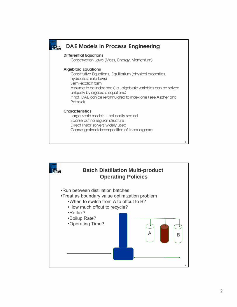
Batch Distillation Multi-product Operating Policies
5XQ�EHWZHHQ�GLVWLOODWLRQ�EDWFKHV7UHDW�DV�ERXQGDU\�YDOXH�RSWLPL]DWLRQ�SUREOHP
:KHQ�WR�VZLWFK�IURP�$�WR�RIIFXW WR�%"+RZ�PXFK�RIIFXW WR�UHF\FOH"5HIOX["%RLOXS 5DWH"2SHUDWLQJ�7LPH"
$ %

3
5
Catalytic Cracking of Gasoil (Tjoa, 1991)
number of states and ODEs: 2number of parameters:3no control profilesconstraints: pL � p � pU
Objective Function: Ordinary Least Squares
(p1, p2, p3)0 = (6, 4, 1)(p1, p2, p3)* = (11.95, 7.99, 2.02)(p1, p2, p3)true = (12, 8, 2)
1.00.80.60.40.20.0
0.0
0.2
0.4
0.6
0.8
1.0
YA_data
YQ_data
YA_estimate
YQ_estimate
t
Yi
Parameter Estimation
0)0( ,1)0(
)(
, ,
22
1
231
321
==−−=
+−=
→→→
qa
qpapq
appa
SASQQA ppp
�
�
6
Optimization of dynamic batch process operation resulting from reactor and distillation column
DAE models:z’ = f(z, y, u, p)g(z, y, u, p) = 0
number of states and DAEs: nz + nyparameters for equipment design (reactor, column)nu control profiles for optimal operation
Constraints: uL � u(t) � uU zL � z(t) � zU
yL � y(t) � yU pL � p � pU
Objective Function: amortized economic function at end of cycle time tf
zi,I0 zi,II
0zi,III0 zi,IV
0
zi,IVf
zi,If zi,II
f zi,IIIf
Bi
A+B→C
C+B→P+E
P+C→G
5
10
15
20
25
580
590
600
610
620
630
640
0 0.5 1 1.5 2 2.50 0.25 0.5 0.75 1 1.25Time (h r.)
Dyn a m ic
C o nsta nt
Dyn a mic
C o nsta nt
optimal reactor temperature policy optimal column reflux ratio
Batch Process Optimization

4
7
Nonlinear Model Predictive Control (NMPC)
Process
NMPC Controller
d : disturbancesz : differential statesy : algebraic states
u : manipulatedvariables
ysp : set points
( )( )dpuyzG
dpuyzFz
,,,,0
,,,,
==′
NMPC Estimation and Control
NMPC Subproblem
Why NMPC?
� Track a profile
� Severe nonlinear dynamics (e.g, sign changes in gains)
� Operate process over wide range (e.g., startup and shutdown)
Model Updater( )( )dpuyzG
dpuyzFz
,,,,0
,,,,
==′
sConstraintOther
sConstraint Bound
0init
212sp
z)t(z)t),t(),t(y),t(z(G
)t),t(),t(y),t(z(F)t(z.t.s
||))||||y)t(y||minuy Q
kkQ
==
=′
−+−∑ ∑ −
u
u
u(tu(tu
8
tf, final timeu, control variablesp, time independent parameters
t, timez, differential variablesy, algebraic variables
Dynamic Optimization Dynamic Optimization ProblemProblem
( )ftp,u(t),y(t),z(t), min Φ
( )pttutytzfdt
tdz,),(),(),(
)( =
( ) 0,),(),(),( =pttutytzg
ul
ul
ul
ul
o
ppp
utuu
ytyy
ztzz
zz
dd
dd
dd
dd
)(
)(
)(
)0(
s.t.

5
9
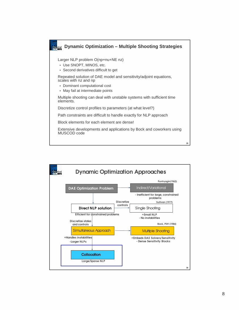
Dynamic Optimization Approaches
DAE Optimization Problem
Multiple Shooting
+Embeds DAE Solvers/Sensitivity- Dense Sensitivity Blocks
+Handles instabilities
Single Shooting
Sullivan (1977)
+Small NLP - No instabilities
Discretize controls
Collocation
Large/Sparse NLP
Direct NLP solution
Efficient for constrained problems
Simultaneous Approach
-Larger NLPs
Discretize states and controls
Indirect/Variational
Pontryagin(1962)
- Inefficient for large, constrained problems
Bock, Plitt (1984)
10
Sequential Approaches - Parameter Optimization
Consider a simpler problem without control profiles:
e.g., equipment design with DAE models - reactors, absorbers, heat exchangers
Min Φ (z(tf))
z’ = f(z, p), z (0) = z0
g(z(tf)) � 0, h(z(tf)) = 0
By treating the ODE model as a "black-box" a sequential algorithm can be constructed that can be treated as a nonlinear program.
Task: How are gradients calculated for optimizer?
NLPSolver
ODEModel
GradientCalculation
P
φ,g,h
z (t)

6
11
Gradient Calculation
Perturbation
Sensitivity Equations
Adjoint Equations
Perturbation
Calculate approximate gradient by solving ODE model (np + 1) times
Let ψ = Φ, g and h (at t = tf)
dψ/dpi = {ψ (pi + ̈ pi) - ψ (pi)}/ ¨pi
Very simple to set up
Leads to poor performance of optimizer and poor detection of optimum unless roundoff error (O(1/¨pi) and truncation error (O(̈pi)) are small.
Work is proportional to np (expensive)
12
Direct Sensitivity
From ODE model:
(nz x np sensitivity equations)
• z and si , i = 1,…np, an be integrated forward simultaneously.
• for implicit ODE solvers, si(t) can be carried forward in time after converging on z
• linear sensitivity equations exploited in ODESSA, DASSAC, DASPK, DSL48s and a number of other DAE solvers
Sensitivity equations are efficient for problems with many more constraints than parameters (1 + ng + nh > np)
{ }
iii
T
iii
ii
p
zss
z
f
p
fs
dt
ds
ip
tzts
pzztpzfzp
∂∂=
∂∂+
∂∂==′
=∂
∂=
==′∂∂
)0()0( ,)(
...np 1, )(
)( define
)()0(),,,( 0

7
13
Multiple Shooting for Dynamic Optimization
Divide time domain into separate regions
Integrate DAEs state equations over each region
Evaluate sensitivities in each region as in sequential approach wrt uij, p and zj
Impose matching constraints in NLP for state variables over each region
Variables in NLP are due to control profiles as well as initial conditions in each region
14
Multiple ShootingNonlinear Programming Problem
uL
x
xxx
xc
xfn
≤≤
=
ℜ∈
0)(s.t
)(min
( ))(),( min,,
ffpu
tytzji
ψ
( ) z)z(tpuyzfdt
dzjjji ==
,,,, ,
( ) 0,ji, =pz,y,ug
ul
uiji
li
ukkjij
lk
ukkjij
lk
jjjij
ppp
uuu
ytpuzyy
ztpuzzz
ztpuzz
≤≤
≤≤
≤≤
≤≤
=− ++
,
,
,
11,
),,,(
),,,(
0),,,(s.t.
(0)0 zzo = Solved Implicitly
8
15
Dynamic Optimization – Multiple Shooting Strategies
Larger NLP problem O(np+nu+NE nz) • Use SNOPT, MINOS, etc.• Second derivatives difficult to get
Repeated solution of DAE model and sensitivity/adjoint equations, scales with nz and np
• Dominant computational cost• May fail at intermediate points
Multiple shooting can deal with unstable systems with sufficient time elements.
Discretize control profiles to parameters (at what level?)
Path constraints are difficult to handle exactly for NLP approach
Block elements for each element are dense!
Extensive developments and applications by Bock and coworkers using MUSCOD code
16
Dynamic Optimization Approaches
DAE Optimization Problem
Multiple Shooting
+Embeds DAE Solvers/Sensitivity- Dense Sensitivity Blocks
+Handles instabilities
Single Shooting
Sullivan (1977)
+Small NLP - No instabilities
Discretize controls
Collocation
Large/Sparse NLP
Direct NLP solution
Efficient for constrained problems
Simultaneous Approach
-Larger NLPs
Discretize states and controls
Indirect/Variational
Pontryagin(1962)
- Inefficient for large, constrained problems
Bock, Plitt (1984)
9
17
Nonlinear DynamicOptimization Problem
Collocation onfinite Elements
Continuous variables
Nonlinear ProgrammingProblem (NLP)
Discretized variables
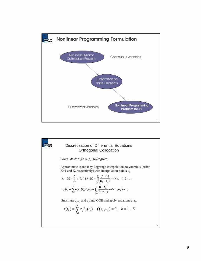
Nonlinear Programming Formulation
18
Discretization of Differential Equations Orthogonal Collocation
Given:dz/dt = f(z, u, p), z(0)=given
Approximate z and u by Lagrange interpolation polynomials (order K+1 and K, respectively) with interpolation points, tk
kkNjk
jK
kjj
k
K
kkkK
kkNjk
jK
kjj
k
K
kkkK
ututt
ttttutu
ztztt
ttttztz
===>−−
∏==
===>−−
∏==
≠==
+
≠==
+
∑
∑
)()(
)()(,)()(
)()(
)()(,)()(
11
100
1
""
""
Substitute zN+1 and uN into ODE and apply equations at tk.Substitute zN+1 and uN into ODE and apply equations at tk.
Kkuzftztr kk
K
jkjjk ,...1 ,0),()()(
0
==−= ∑=
"�

10
19
z(t)
z N+1(t)
Sta
te P
rofile
t ft 1 t 2 t 3
r(t)
t 1 t 2 t 3
Min φ(z(tf))s.t. z’ = f(z, u, p), z(0)=z0
g(z(t), u(t), p) � 0h(z(t), u(t), p) = 0
to Nonlinear Program
How accurate is approximation
Converted Optimal Control Problem
Using Collocation
0)1(
,...1
0
0
z(0) ,0),()(
0
00
=−
=
=≤
==−
∑
∑
=
=
f
K
jjj
kk
kk
kk
K
jkjj
f
zz
Kk
),uh(z
),ug(z
zuzftz
)(z Min
"
"�
φ
20
to tf
u u u u
Collocation points
• ••• •
•• •
•••
•
Polynomials
u uu u
•
Finite element, i
ti
Mesh points
hi
u u u u
∑=
=K
qiqq(t) zz(t)
0
"
u uu
u
element i
q = 1q = 1
q = 2 q = 2
uuuuContinuous Differential variables
Discontinuous Algebraic and
Control variables
u
u
u u
Collocation on Finite ElementsCollocation on Finite Elements
∑=
=K
qiqq(t) yy(t)
1
" ∑=
=K
qiqq(t) uu(t)
1
"
τd
dz
hdt
dz
i
1=
),( uzfhd
dzi=
τ
NE 1,.. i 1,..K,k ,0),,())(()(0
===−= ∑=
K
jikikikjijik puzfhztr τ"�
]1,0[,1
1’’ ∈+= ∑
−
=
ττ ji
i
iiij hht

11
21
Nonlinear Programming ProblemNonlinear Programming Problem
uL
x
xxx
xc
xfn
≤≤
=
ℜ∈
0)(s.t
)(min( )fzψ min
( ) 0,, ,,, =p,uyzg kikiki
ul
ujiji
lji
uji
lji
ul
ppp
uuu
yyy
zzz
≤≤
≤≤
≤≤
≤≤
,,,
,ji,,
ji, ji,ji,
s.t. ∑=
=−K
jikikikjij puzfhz
0
0),,())(( τ"�
)0( ,0))1((
,..2 ,0))1((
100
,
00,1
zzzz
NEizz
K
jfjjNE
K
jijji
==−
==−
∑
∑
=
=−
"
"
Finite elements,hi, can also be variable to determine break points for u(t).
Add hu � hi � 0, Σ hi=tf
Can add constraints g(h, z, u) � ε for approximation error
22
Theoretical Properties of Simultaneous Method
A. Stability and Accuracy of Orthogonal Collocation
• Equivalent to performing a fully implicit Runge-Kuttaintegration of DAE models at Gaussian (Radau) points
• 2K order (2K-1) method which uses K collocation points• Algebraically stable (i.e., possesses A, B, AN and BN stability)
B. Analysis of the Optimality Conditions (Kameswaran, B., 2007)
• An equivalence has been established between the KKT conditions of NLP and the variational necessary conditions
• Rates of convergence have been established for the NLP method

12
23
A B
C
u
u /22
u(T(t))
Example: Batch reactor - temperature profile
Maximize yield of B after one hour’s operation by manipulating a transformed temperature, u(t).
⇒ Minimize -zB(1.0)s.t.
z’A = -(u+u2/2) zA
z’B = u zA
zA(0) = 1zB(0) = 00 � u(t) � 5
Optimality conditions:H = -λA(u+u2/2) zA + λB u zA
∂H/∂u = λA (1+u) zA + λB zAλ’A = λA(u+u2/2) - λB u, λA(1.0) = 0λ’B = 0, λB(1.0) = -1
24
Op
tim
al P
rofile
, u
(t)
0. 0.2 0.4 0.6 0.8 1.0
2
4
6
Time, h
Results:Piecewise Linear Approximation with Variable Time ElementsOptimum B/A: 0.5726Equivalent # of ODE solutions: 32
Batch Reactor Optimal Temperature Program Piecewise Linear

13
25
Op
tim
al P
rofile
, u
(t)
0. 0.2 0.4 0.6 0.8 1.0
2
4
6
Time, h
Results:Control Vector Iteration with Conjugate GradientsOptimum (B/A): 0.5732Equivalent # of ODE solutions: 58
Batch Reactor Optimal Temperature Program
Indirect Approach
26
Results of Optimal Temperature Program Batch Reactor (Revisited)
Results- NLP with Orthogonal CollocationOptimum B/A - 0.5728# of ODE Solutions - 0.7(Equivalent)

14
27
Dynamic Optimization Engines
Evolution of NLP Solvers:
Î for dynamic optimization, control and estimation
E.g., NPSOL and Sequential Dynamic Optimization - over 100 variables and constraints
SQP
28
Dynamic Optimization Engines
Evolution of NLP Solvers:
Î for dynamic optimization, control and estimation
E.g, SNOPT and Multiple Shooting - over 100 d.f.s but over 105 variables and constraints
SQP rSQP

15
29
Dynamic Optimization Engines
Evolution of NLP Solvers:
Î for dynamic optimization, control and estimation
E.g., NPSOL and Sequential Dynamic Optimization - over 100 variables and constraints E.g, SNOPT and Multiple Shooting - over 100 d.f.s but over 105 variables and constraintsE.g., IPOPT - Simultaneous dynamic optimizationover 1 000 000 variables and constraints
SQP rSQP Full-spaceBarrier
Object Oriented Codes tailored to structure, sparse linearalgebra and computer architecture (e.g., IPOPT 3.3)
30
Barrier Methods for Large-Scale Nonlinear Programming
0
0)(s.t
)(min
≥=
ℜ∈
x
xc
xfnx
Original Formulation
0)(s.t
ln)()( min1
=
−= ∑=ℜ∈
xc
xxfxn
ii
x nµϕµBarrier Approach
Can generalize for
bxa ≤≤
⇒ As µ Î 0, x*(µ) Î x* Fiacco and McCormick (1968)

16
31
Solution of the Barrier Problem
⇒ Newton Directions (KKT System)
0 )(
0
0 )()(
==−=−+∇
xc
eXv
vxAxf
µλ
⇒ Solve
−
−+∇−=
−
eXv
c
vAf
d
d
d
XV
A
IAW x
T
0
00
µ
λ
ν
λ
IPOPT Code IPOPT Code –– www.coinwww.coin --or.orgor.org
)(
...]1 ,1 ,1[
xdiagX
eT
==
32
Solution of the Barrier Problem
⇒ Newton Directions (KKT System)
0 )(
0
0 )()(
==−=−+∇
xc
eXv
vxAxf
µλ
⇒ Solve
−
−+∇−=
−
eXv
c
vAf
d
d
d
XV
A
IAW x
T
0
00
µ
λ
ν
λ
⇒ Reducing the Systemxv VdXveXd 11 −− −−=µ
∇−=
Σ++ c
d
A
AW x
T
µϕλ
0 VX 1−=Σ
IPOPT Code IPOPT Code –– www.coinwww.coin --or.orgor.org
)(
...]1 ,1 ,1[
xdiagX
eT
==
17
33
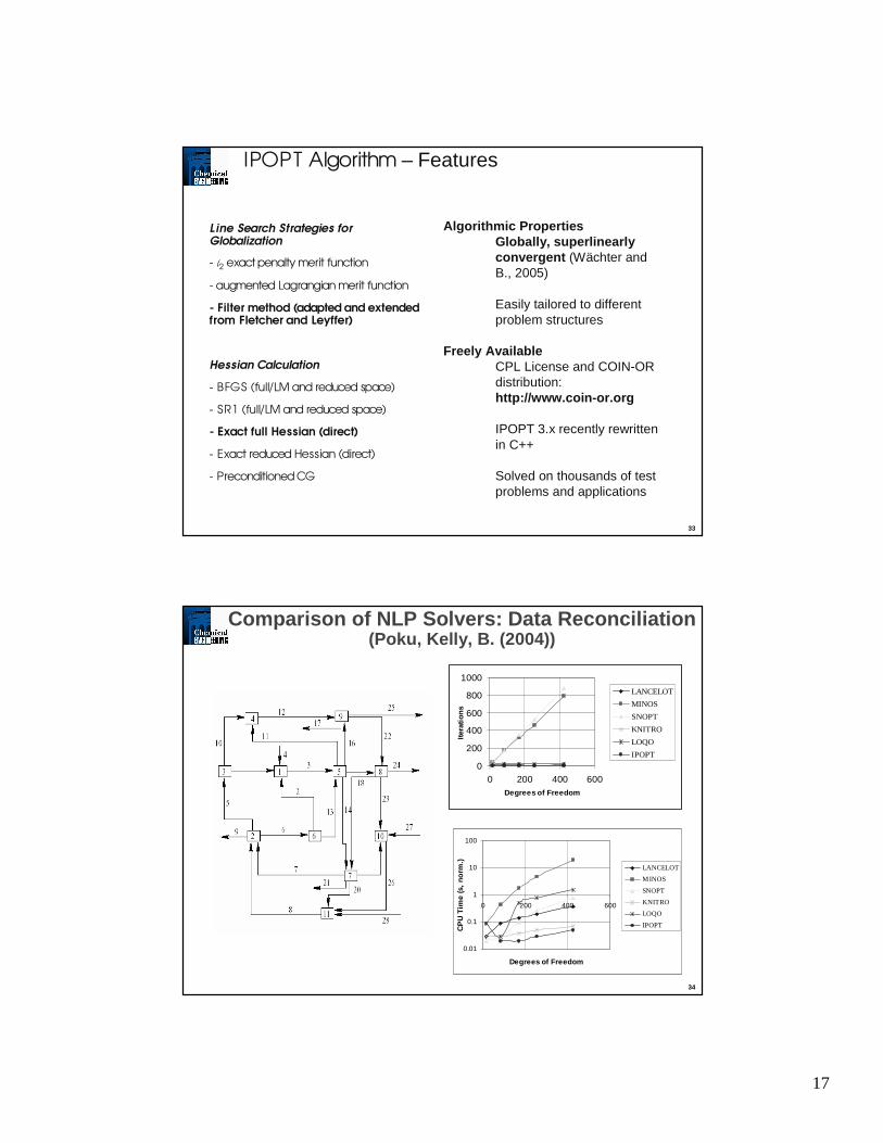
IPOPT Algorithm – Features
Line Search Strategies for Globalization
- l2 exact penalty merit function
- augmented Lagrangian merit function
- Filter method (adapted and extended from Fletcher and Leyffer)
Hessian Calculation
- BFGS (full/LM and reduced space)
- SR1 (full/LM and reduced space)
- Exact full Hessian (direct)
- Exact reduced Hessian (direct)
- Preconditioned CG
Algorithmic PropertiesGlobally, superlinearlyconvergent (Wächter and B., 2005)
Easily tailored to different problem structures
Freely AvailableCPL License and COIN-OR distribution: http://www.coin-or.org
IPOPT 3.x recently rewritten in C++
Solved on thousands of test problems and applications
34
Comparison of NLP Solvers: Data Reconciliation(Poku, Kelly, B. (2004))
0.01
0.1
1
10
100
0 200 400 600
Degrees of Freedom
CP
U T
ime
(s,
norm
.) LANCELOT
MINOS
SNOPT
KNITRO
LOQO
IPOPT
0
200
400
600
800
1000
0 200 400 600Degrees of Freedom
Itera
tions
LANCELOT
MINOS
SNOPT
KNITRO
LOQO
IPOPT

18
35
Comparison of Computational Complexity(α ∈ [2, 3], β ∈ [1, 2], nw, nu - assume Nm = O(N))
((nu + nw)N)------Backsolve
((nu + nw)N)β(nu N)α(nu N)αStep Determination
---nw3 N---NLP Decomposition
N (nu + nw)(nw N) (nu + nw)2(nw N) (nu N)2Exact Hessian
N (nu + nw)(nw N) (nu + nw)(nw N) (nu N)Sensitivity
---nwβ Nnw
β NDAE Integration
SimultaneousMultiple Shooting
Single Shooting
O((nuN)α + N2nwnu
+ N3nwnu2)
O((nuN)α + N nw3
+ N nw (nw +nu)2)
O((nu + nw)N)β
36
Case Studies• Reactor - Based Flowsheets• Fed-Batch Penicillin Fermenter• Temperature Profiles for Batch Reactors• Parameter Estimation of Batch Data• Synthesis of Reactor Networks• Batch Crystallization Temperature Profiles• Ramping for Continuous Columns• Reflux Profiles for Batch Distillation and Column Design• Air Traffic Conflict Resolution• Satellite Trajectories in Astronautics• Batch Process Integration• Source Detection for Municipal Water Networks• Optimization of Simulated Moving Beds• Grade Transition of Polymerization Processes• Parameter Estimation of Tubular Reactors• Nonlinear MPC
Simultaneous DAE Optimization

19
37
Production of High Impact Polystyrene (HIPS)Startup and Transition Policies (Flores et al., 2005a)
Catalyst
Monomer, Transfer/Term. agents
Coolant
Polymer
38
Upper Steady−State
Bifurcation Parameter
System State
Lower Steady−State
Medium Steady−State
Phase Diagram of Steady States
Transitions considered among all steady state pairs

20
39
Upper Steady−State
Bifurcation Parameter
System State
Lower Steady−State
Medium Steady−State
Phase Diagram of Steady States
Transitions considered among all steady state pairs
0 0.5 1 1.5 2 2.5 3 3.5 4 4.5 5
300
350
400
450
500
550
600
N1
N2
N3
A1
A4
A2
A3
A5
Cooling water flowrate (L/s)
Te
mp
era
ture
(K
)
1: Qi = 0.00152: Qi = 0.00253: Qi = 0.0040
3
2
1
0 0.02 0.04 0.06 0.08 0.1 0.12
300
350
400
450
500
550
600
650
Initiator flowrate (L/s)
Te
mp
era
ture
(K
)
1: Qcw = 102: Qcw = 1.03: Qcw = 0.1
32 1
3
2
1
N2
B1 B2 B3
C1C2
40
0 0.5 1 1.5 20
0.5
1x 10
−3
Time [h]
Initi
ator
Con
c. [m
ol/l]
0 0.5 1 1.5 24
6
8
10
Time [h]
Mon
omer
Con
c. [m
ol/l]
0 0.5 1 1.5 2300
350
400
Time [h]
Rea
ctor
Tem
p. [
K]
0 0.5 1 1.5 2290
300
310
320
Time [h]
Jack
et T
emp.
[K
]
0 20 40 60 80 1000
0.5
1
1.5x 10
−3
Time [h]
Initi
ator
Flo
w. [
l/sec
]
0 0.5 1 1.5 20
0.5
1
Time [h]Coo
ling
wat
er F
low
. [l/s
ec]
0 0.5 1 1.5 20
1
2
3
Time [h]
Fee
drat
e F
low
. [l/s
ec]
• 926 variables• 476 constraints• 36 iters. / 0.95 CPU s (P4)
Startup to Unstable Steady State

21
41
HIPS Process Plant (Flores et al., 2005b)
•Many grade transitions considered with stable/unstable pairs
•1-6 CPU min (P4) with IPOPT
•Study shows benefit for sequence of grade changes to achieve wide range of grade transitions.
42
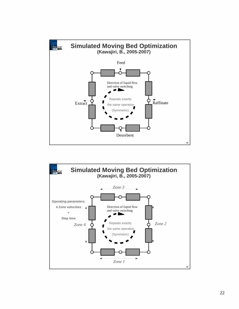
Simulated Moving Bed Optimization(Kawajiri, B., 2005-2007)
Direction of liquid flowand valve switching
Feed Raffinate
DesorbentExtract
22
43
Simulated Moving Bed Optimization(Kawajiri, B., 2005-2007)
Direction of liquid flowand valve switching
Feed
Raffinate
Desorbent
ExtractRepeats exactly
the same operation
(Symmetric)
44
Simulated Moving Bed Optimization(Kawajiri, B., 2005-2007)
Direction of liquid flowand valve switching
Repeats exactly
the same operation
(Symmetric)
Operating parameters:
4 Zone velocities
+
Step time
Zone 4 Zone 2
Zone 3
Zone 1
23
45
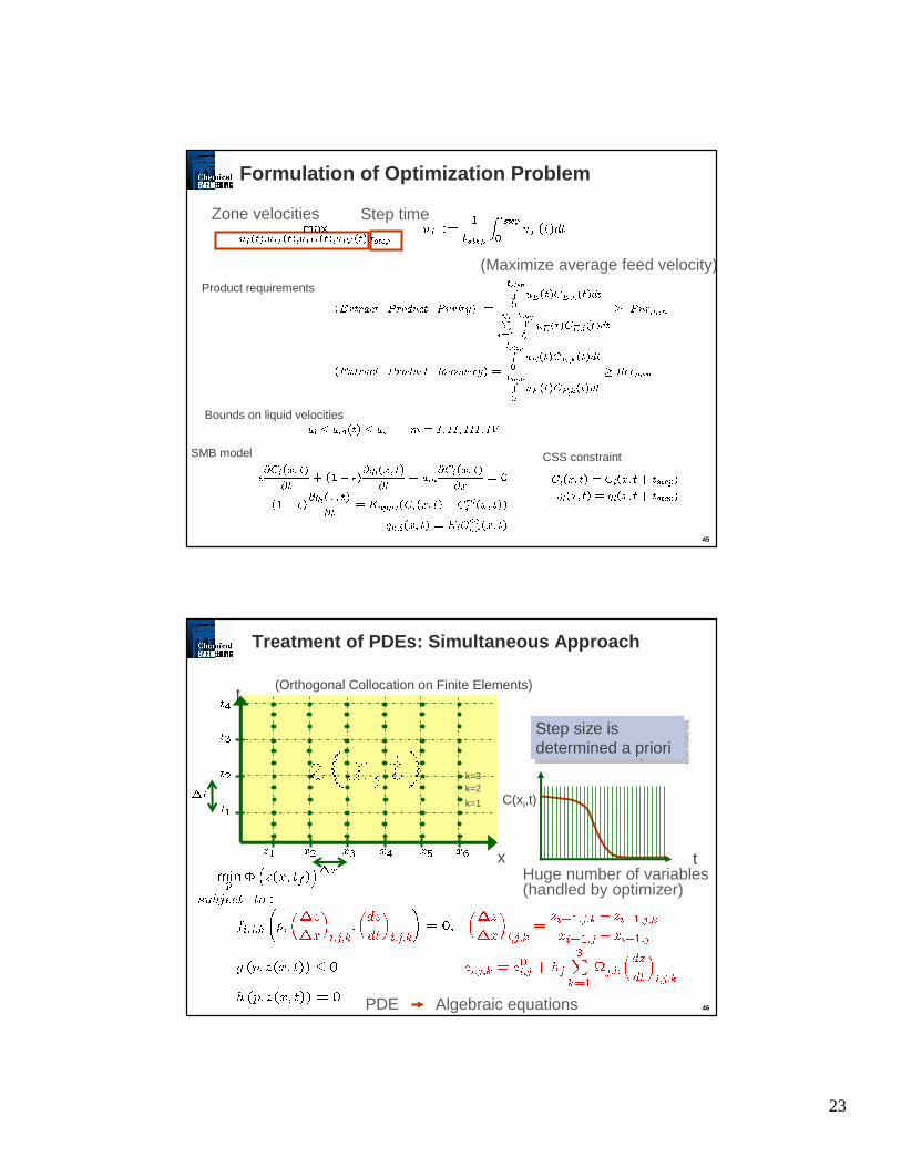
Formulation of Optimization Problem
Zone velocities Step time
(Maximize average feed velocity)
Bounds on liquid velocities
Product requirements
CSS constraintSMB model
46
Treatment of PDEs: Simultaneous Approach
t
x
(Orthogonal Collocation on Finite Elements)
k=1
k=2k=3
Algebraic equations PDE
Step size is determined a priori
Step size is determined a priori
tHuge number of variables (handled by optimizer)
C(xi,t)

24
47
Comparison of two approaches
CPU Time*
Sequential Approach 111.8 min
1.53 minSimultaneous Approach
# of iteration
49
47
0 1 2 3 4 5 6 7 8−0.1
0
0.1
0.2
0.3
0.4
0.5
0.6
0.7
0.8
x [m]
Nor
mal
ized
Con
cenr
atio
n, C
i(x,t st
ep)/
CF
,i
Comp.1 Single discretizationComp.2 Single discretizationComp.1 Full discretizationComp.2 Full discretization Sequential and Simultaneous
methods find same optimal solution
# of variables
33999
644Implemented on gPROMS, solved using SRQPDImplemented on gPROMS, solved using SRQPD
Implemented on AMPL, solved using IPOPTImplemented on AMPL, solved using IPOPT
*On Pentium IV 2.8GHz
(89% spent by integrator)
(Linear isotherm, fructose/glucose separation)
Initial feed velocity: 0.01 m/h
Optimal feed velocity: 0.52 m/h
Optimization
48
z Standard SMB
Nonstandard SMB: Addressed by Extended Superstructure NLP
z Three Zone
(Circulation loop is cut open)
z VARICOL
(Asynchronous switching)
25
49
0 2 4 6 80
0.5
1
x [m]
Ci(x
,t)/C
F,i →
8.000 m/h
⇓u
D1 =8.000m/h
t/tstep
= 0.142
→8.000 m/h
t/tstep
= 0.142
→8.000 m/h
⇓ uR3 =8.000m/h
t/tstep
= 0.142
→8.000 m/h
⇓u
D4 =8.000m/h
⇓ uE4=8.000m/h
t/tstep
= 0.142
0 2 4 6 80
0.5
1
x [m]
Ci(x
,t)/C
F,i →
7.916 m/h
⇓u
D1 =7.916m/h
t/tstep
= 0.334
→7.916 m/h
t/tstep
= 0.334
→7.916 m/h
⇓ uR3 =7.916m/h
t/tstep
= 0.334
→8.000 m/h
⇓u
D4 =8.000m/h
⇓ uE4=8.000m/h
t/tstep
= 0.334
0 2 4 6 80
0.5
1
x [m]
Ci(x
,t)/C
F,i →
8.000 m/h
⇓u
D1 =8.000m/h
t/tstep
= 0.434
→8.000 m/h
t/tstep
= 0.434
→8.000 m/h
t/tstep
= 0.434
→8.000 m/h
⇓ uE4=8.000m/h
t/tstep
= 0.434
0 2 4 6 80
0.5
1
x [m]
Ci(x
,t)/C
F,i →
6.332 m/h
⇓u
D1 =6.332m/h
t/tstep
= 0.800
→6.332 m/h
t/tstep
= 0.800
→8.000 m/h
⇓u
F3=1.668m/h
t/tstep
= 0.800
→8.000 m/h
⇓ uE4=8.000m/h
t/tstep
= 0.800
0 2 4 6 80
0.5
1
x [m]
Ci(x
,t)/C
F,i →
8.000 m/h
⇓u
D1 =8.000m/h
⇓ uE1=3.757m/h
t/tstep
= 1.000
→4.243 m/h
t/tstep
= 1.000
→8.000 m/h
⇓u
F3=3.757m/h
t/tstep
= 1.000
→8.000 m/h
⇓ uR4 =8.000m/h
t/tstep
= 1.000
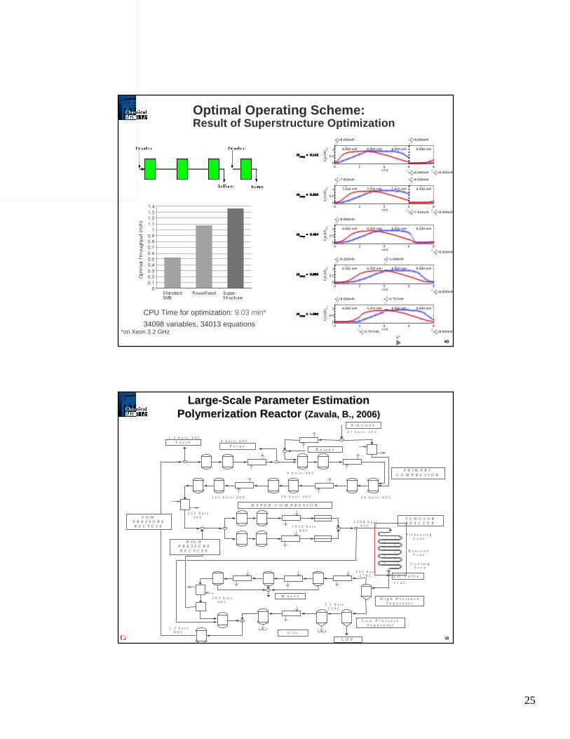
Optimal Operating Scheme:Result of Superstructure Optimization
Standard SMB
PowerFeed Super -Structure
0
0.1
0.2
0.3
0.4
0.5
0.6
0.7
0.8
0.9
1
1.1
1.2
1.3
1.4
Op
tim
al
Th
rou
gh
pu
t [m
/h]
CPU Time for optimization: 9.03 min*
34098 variables, 34013 equations *on Xeon 3.2 GHz
50
Parameter Estimation
Model Development - Kinetics
Product Properties Correlations
On-line Implementation - DisturbancesHeat-transfer, Impurities
},...,,,,,,,{ dcpsmi ttfffpIik ∈
LargeLarge --Scale Rigorous Reactor ModelScale Rigorous Reactor Model
Reactor Operating ConditionsReactor Operating Conditions
Polymer Properties (Melt Index)Polymer Properties (Melt Index)
Kinetic Mechanism (Free-Radical)
Reaction Rates
Method of Moments Monomer(s)
Initiator(s)
Solvent(s), CTA(s)
Moments NCLD
Material & Energy ODEsPDEs
Type & ConfigurationSteady-State vs. Dynamic
RigorousPTT Properties
ViscosityHeat Capacity
DensityTransport
MonomerComonomer
Initiator(s)
1 2 3 NZ
LargeLarge --Scale Parameter EstimationScale Parameter EstimationPolymerization Reactor Polymerization Reactor (Zavala, B., 2006)(Zavala, B., 2006)
H I G HP R E S S U R ER E C Y C L E
L O WP R E S S U R ER E C Y C L E
E t h y l e n e
B u t a n eP u r g e
T o r c h
P R I M A R YC O M P R E S S O R
H Y P E R - C O M P R E S S O R
T U B U L A RR E A C T O R
L D P
W a x e s
2 7 b a r s / 2 5 C
6 b a r s / 4 0 C1 . 5 b a r s / 4 0 C
6 b a r s / 4 0 C
2 4 b a r s / 4 0 C5 6 b a r s / 4 0 C1 0 3 b a r s / 4 0 C
2 5 5 b a r s4 0 C
1 0 1 0 b a r s4 0 C
2 2 0 0 b a r s8 5 C
P r e h e a t i n gZ o n e
R e a c t i o nZ o n e
C o o l i n gZ o n e
2 . 5 b a r s2 2 0 C
1 . 5 b a r s4 0 C
2 8 5 b a r s4 0 C
L D V a l v e
2 7 4 C
3 5 0 b a r s2 7 0 C
O i l s
H i g h P r e s s u r eS e p a r a t o r
L o w P r e s s u r eS e p a r a t o r

26
51
MonomerComonomer
Initiator(s)
1 2 3 NZ
z z z z
Material & Energy
Physical Properties
Zone Transitions
8 Stiffness + Highly Nonlinear + Parametric Sensit ivity + Algebraic Coupling
500 ODEs1000 AEs
LargeLarge --Scale Parameter EstimationScale Parameter Estimation
52
LargeLarge --Scale Parameter EstimationScale Parameter Estimation
~ 35 Elementary Reactions~100 Kinetic Parameters
� Complex Kinetic Mechanisms

27
53
LargeLarge --Scale Parameter EstimationScale Parameter Estimation
� Parameter Estimation for Industrial Applications
� Use Rigorous Model to Match Plant Data Directly
� Start with Standard Least-Squares Formulation
Rigorous Reactor Model
� Special Case of Multi-Stage Dynamic Optimization Pr oblem
� Solve using Simultaneous Collocation-Based Approach
Least-Squares
1 data set 6 data setsx 6500 ODEs
1000 AEs3000 ODEs6000 AEs
54
� Multi-Zone Tubular Reactor – Quasi Steady-State
� Data Sets: Operating Conditions and Properties for Different Grades
� Match: Temperature Profiles and Product Properties
� On-line Adjusting Parameters Æ Track Evolution of Disturbances
� Kinetic Parameters Æ Development and Discrimination among Rigorous Models
� Results
� Single Data Set (On-line Adjusting Parameters)
� Multiple Data Sets (On-line Adjusting Parameters + Kinetics)
Bottleneck (Memory Requirements) Factorization Step
LargeLarge --Scale Parameter EstimationScale Parameter Estimation
28
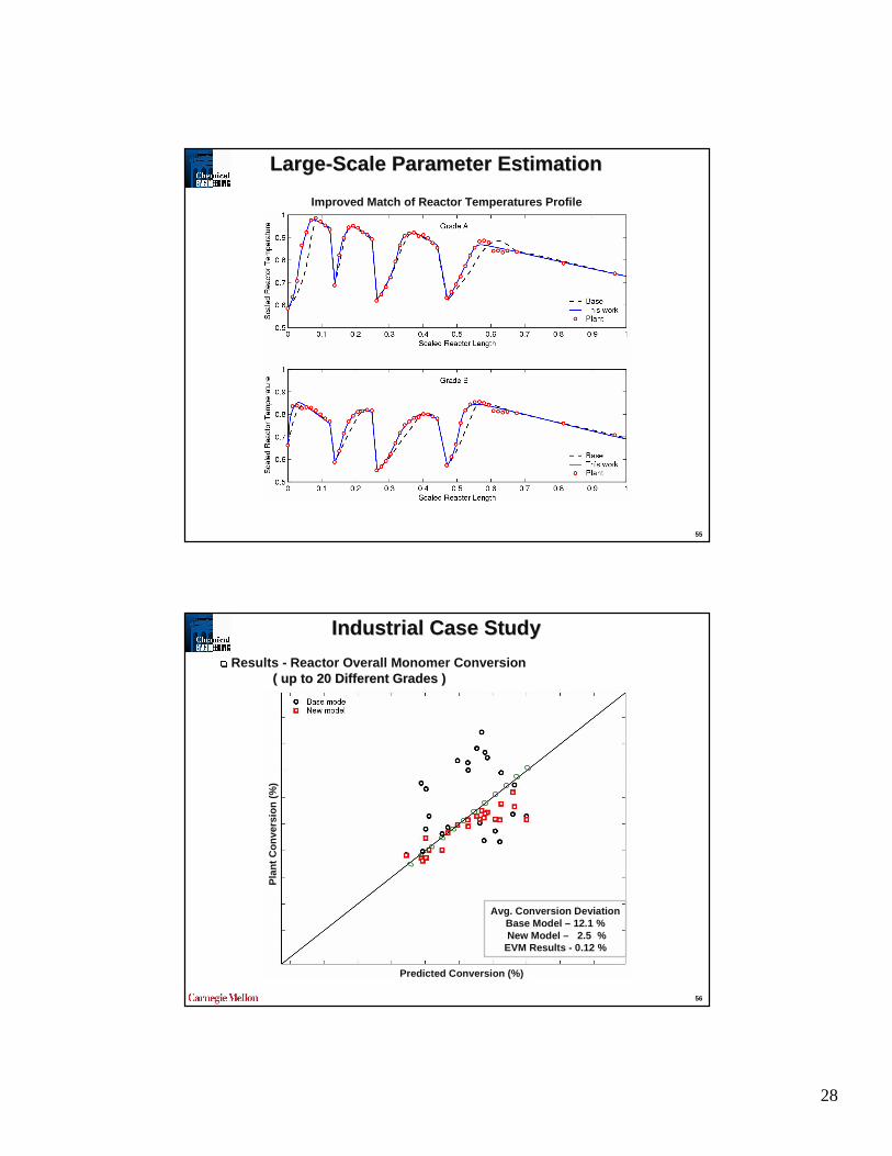
55
Improved Match of Reactor Temperatures Profile
LargeLarge --Scale Parameter EstimationScale Parameter Estimation
56
Industrial Case StudyIndustrial Case Study
� Results - Reactor Overall Monomer Conversion ( up to 20 Different Grades )( up to 20 Different Grades )
Avg. Conversion DeviationBase Model – 12.1 %New Model – 2.5 %
EVM Results - 0.12 %
Predicted Conversion (%)
Pla
nt C
onve
rsio
n (%
)
29
57
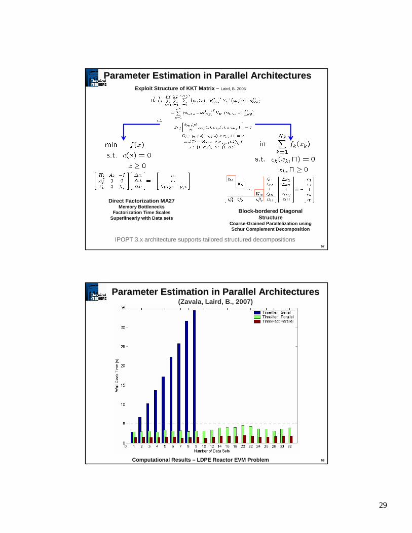
Exploit Structure of KKT Matrix – Laird, B. 2006
Parameter Estimation in Parallel Architectures Parameter Estimation in Parallel Architectures
Direct Factorization MA27Memory Bottlenecks
Factorization Time Scales Superlinearly with Data sets
Block-bordered Diagonal Structure
Coarse-Grained Parallelization using Schur Complement Decomposition
IPOPT 3.x architecture supports tailored structured decompositions
58Computational Results – LDPE Reactor EVM Problem
Parameter Estimation in Parallel ArchitecturesParameter Estimation in Parallel Architectures(Zavala, Laird, B., 2007)

30
59
Supply Chain, Planning and Scheduling• Large LP and MILP models• Many Discrete Decisions• Few Nonlinearities• Essential link needed to process models• Decisions need to be feasible at lower levels
Planning
Scheduling
Site-wide Optimization
Real-time Optimization
Model Predictive Control
Regulatory Control
Fe
asi
bili
ty
Pe
rfo
rma
nc
e
Decision-making in Chemical Industries
60
Real-time Optimization and Advanced Process Control• Fewer discrete decisions• Many nonlinearities• Frequent, “on-line” time-critical solutions• Higher level decisions must be feasible• Performance communicated for higher level decisions
Planning
Scheduling
Site-wide Optimization
Real-time Optimization
Model Predictive Control
Regulatory Control
Fe
asi
bili
ty
Pe
rfo
rma
nc
e
Decision Pyramid for Process Operations
APCMPC ⊂
Off-line (open loop)
On-line (closed loop)

31
61
Dynamic Real-time Optimization Integrate On-line Optimization/Control with Off-line Planning• Consistent, first-principle models• Consistent, long-range, multi-stage planning• Increase in computational complexity • Time-critical calculations
Applications• Batch processes• Grade transitions• Cyclic reactors (coking, regeneration…)
• Cyclic processes (PSA, SMB…)
Continuous processes are never in steady state:
• Feed changes• Nonstandard operations• Optimal disturbance rejections
Simulation environments and first principle dynamic models are widely used for off-line studies
Can these results be implemented directly on-line for large-scale systems?
8
Planning
Scheduling
Site-wide Optimization
Real-time Optimization
Model Predictive Control
Regulatory Control
Fe
asi
bili
ty
Pe
rfo
rma
nc
e
62
Nonlinear Model Predictive Control (NMPC)
Process
NMPC Controller
d : disturbancesz : differential statesy : algebraic states
u : manipulatedvariables
ysp : set points
( )( )dpuyzG
dpuyzFz
,,,,0
,,,,
==′
NMPC Estimation and Control
sConstraintOther
sConstraint Bound
0init
212sp
z)t(z)t),t(),t(y),t(z(G
)t),t(),t(y),t(z(F)t(z.t.s
||))||||y)t(y||minuy Q
kkQ
==
=′
−+−∑ ∑ −
u
u
u(tu(tu
NMPC Subproblem
Why NMPC?
� Track a profile
� Severe nonlinear dynamics (e.g, sign changes in gains)
� Operate process over wide range (e.g., startup and shutdown)
Model Updater( )( )dpuyzG
dpuyzFz
,,,,0
,,,,
==′

32
63
Nonlinear Model Predictive Control (NMPC)
Process
NMPC Controller
d : disturbancesz : differential statesy : algebraic states
u : manipulatedvariables
ysp : set points
( )( )dpuyzG
dpuyzFz
,,,,0
,,,,
==′
NMPC Estimation and Control
sConstraintOther
sConstraint Bound
0init
212sp
z)t(z)t),t(),t(y),t(z(G
)t),t(),t(y),t(z(F)t(z.t.s
||))||||y)t(y||minuy Q
kkQ
==
=′
−+−∑ ∑ −
u
u
u(tu(tu
NMPC Subproblem
Why NMPC?
� Track a profile
� Severe nonlinear dynamics (e.g, sign changes in gains)
� Operate process over wide range (e.g., startup and shutdown)
Model Updater( )( )dpuyzG
dpuyzFz
,,,,0
,,,,
==′
64
Tennessee Eastman Process(Downs and Vogel, 1993)
Unstable Reactor
11 Controls; Product, Purge streams
Model extended with energy balances

33
65
Tennessee Eastman NMPC Model(Jockenhövel, Wächter, B., 2003)
Method of Full Discretization of State and Control Variables
Large-scale Sparse block-diagonal NLP
11Difference (control variables)
141Number of algebraic equations
152Number of algebraic variables
30Number of differential equations
DAE Model
14700Number of nonzeros in Hessian
49230Number of nonzeros in Jacobian
540Number of upper bounds
780Number of lower bounds
10260Number of constraints
109200
Number of variablesof which are fixed
NLP Optimization problem
66
Case Study:Change Reactor pressure by 60 kPa
Control profiles
All profiles return to their base case values
Same production rate
Same product quality
Same control profile
Lower pressure – leads to larger gas phase (reactor) volume
Less compressor load

34
67
Case Study: Change Reactor Pressure by 60 kPa
Optimization with IPOPT
1000 Optimization Cycles
5-7 CPU seconds
11-14 Iterations
Optimization with SNOPT
Often failed due to poor conditioning
Could not be solved within sampling times
> 100 Iterations
68
Limitations to NMPC Implementation
Issues: time-critical, more complex models, fast NLP solvers.
Computational delay – between receipt of process measurement and injection of control, determined by cost of dynamic optimization
Leads to loss of performance and stability (see Findeisen and Allgöwer, 2004; Santos et al., 2001)
As larger As larger NLPsNLPs are considered for NMPC, can are considered for NMPC, can computational delay be overcome?computational delay be overcome?

35
69
Avoid computational delay due to on-line optimization?
Real-time Iteration• preparation, feedback response and transition stages
• solve perturbed (linearized) problem on-line
– Li, de Oliveira, Santos, B. (1990+) – Diehl, Findeisen, Bock, Allgöwer et al. (2000+)– > two orders of magnitude reduction in on-line computation
• solve complete NLP in background (‘between’ sampling times as part of preparation and transition stages
Based on NLP sensitivity for dynamic systems• Extended to Simultaneous Collocation approach – Zavala et al.
(2007)
• Develop Advanced Step NMPC
• Related to MPC with linearization constantly updated one step behind
70
Nonlinear Model Predictive Control Nonlinear Model Predictive Control ––Parametric Problem (Zavala, Laird, B.)Parametric Problem (Zavala, Laird, B.)

36
71
Nonlinear Model Predictive Control Nonlinear Model Predictive Control ––Parametric Problem (Zavala, Laird, B.)Parametric Problem (Zavala, Laird, B.)
72
NLP SensitivityNLP SensitivityParametric Programming
NLP Sensitivity Æ Rely upon Existence and Differentiability of Path
Æ Main Idea: Obtain and find b y Taylor Series Expansion
Optimality Conditions
Solution Triplet

37
73
NLP SensitivityNLP Sensitivity
Optimality Conditions of
Obtaining
Æ Already Factored at Solution
Æ Sensitivity Calculation from Single Backsolve
Æ Approximate Solution Retains Active Set
KKT Matrix IPOPT
Apply Implicit Function Theorem to around
74
Key Concept Key Concept –– Relate to Previous HorizonRelate to Previous Horizon
Solutions to both problems are equivalent in nominal case
(ideal plant model, no disturbances)

38
75
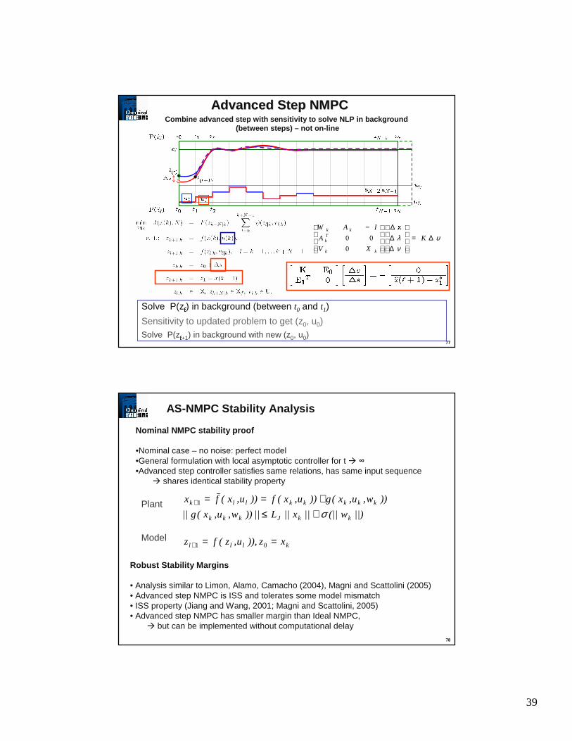
Advanced Step NMPCAdvanced Step NMPCCombine advanced step with sensitivity to solve NLP in background
(between steps) – not on-line
Solve P(z ) in background (between t0 and t1)
υνλ ∆=
∆∆∆
−K
XV
A
IAW
kk
Tk
kk [
0
00
76
Advanced Step NMPCAdvanced Step NMPCCombine advanced step with sensitivity to solve NLP in background
(between steps) – not on-line
Solve P(z ) in background (between t0 and t1)
Sensitivity to updated problem to get (z0, u0)
υνλ ∆=
∆∆∆
−K
XV
A
IAW
kk
Tk
kk [
0
00
39
77
Advanced Step NMPCAdvanced Step NMPCCombine advanced step with sensitivity to solve NLP in background
(between steps) – not on-line
Solve P(z ) in background (between t0 and t1)
Sensitivity to updated problem to get (z0, u0)Solve P(z +1) in background with new (z0, u0)
υνλ ∆=
∆∆∆
−K
XV
A
IAW
kk
Tk
kk [
0
00
78
AS-NMPC Stability Analysis
Nominal NMPC stability proof
•Nominal case – no noise: perfect model•General formulation with local asymptotic controller for t Æ �•Advanced step controller satisfies same relations, has same input sequence
Æ shares identical stability property
klll
kkJkkk
kkkkkllk
xz)),u,z(fz
||)w(|| ||x||L ||))w,u,x(g||
))w,u,x(g))u,x(f))u,x(fx
==
+≤+==
+
+
01
1
σ
Robust Stability Margins
• Analysis similar to Limon, Alamo, Camacho (2004), Magni and Scattolini (2005)• Advanced step NMPC is ISS and tolerates some model mismatch• ISS property (Jiang and Wang, 2001; Magni and Scattolini, 2005) • Advanced step NMPC has smaller margin than Ideal NMPC,
Æ but can be implemented without computational delay
Plant
Model

40
79
CSTR NMPC Example (Hicks and Ray)
• Maintain unstable setpoint• Close to bound constraint• Final time constraint for stability
Effects of:• Computational Delay• Measurement Noise• Model Mismatch• Advanced Step NMPC
80
CSTR NMPC Example – Nominal Case
• NMPC applied with N = 10, τ = 0.5 sampling time• Stable (z = 0) and unstable (z = 0.1) steady states• u2* close to upper bound• Computational delay = 0.5, leads to instabilities

41
81
CSTR NMPC Example – Model Mismatch
Advanced Step NMPC not as robust as ideal - suboptimal selection of u(k)
Better than Direct Variant – due to better active set preservation
0 5 10 15 20 25 30 35 40 45 50
0
0.05
0.1 θ = θnom
− 55%
z c [−]
Time [s]
0 5 10 15 20 25 30 35 40 45 50
0
0.05
0.1 θ = θnom
− 50%
z c [−]
0 5 10 15 20 25 30 35 40 45 50
0
0.05
0.1 θ = θnom
− 40%z c [−
]
0 5 10 15 20 25 30 35 40 45 50
0
0.05
0.1 θ = θnom
− 25%
z c [−]
IdealAdvanced StepDirect
82
CSTR Example: Mismatch + Noise
0 10 20 30 40 50 60 70
0
0.05
0.1σ = 2.5%
θ = θnom
− 50%
z c [−]
IdealAdvanced StepDirect
0 10 20 30 40 50 60 70
0
0.05
0.1σ = 5.0%
z c [−]
0 10 20 30 40 50 60 70
0
0.05
0.1
0.15
σ = 7.5%
z c [−]
Time [s]

42
83
Industrial Case Study – Grade Transition Control
Simultaneous Collocation-BasedApproach
27,135 constraints, 9630 LB & UB
Off-line Solution with IPOPT
Feedback Every 6 min
Process Model: 289 ODEs, 100 AEs
84
NMPC Case Study� Optimal Feedback Policy Æ (On-line Computation 351 CPU s)
Ideal NMPC controller - computational delay not considered
Time delays as disturbances in NMPC
43
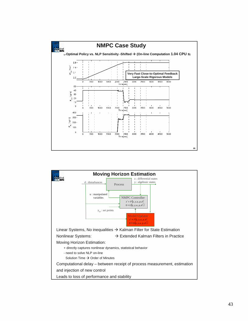
85
NMPC Case Study� Optimal Policy vs. NLP Sensitivity -Shifted Æ (On-line Computation 1.04 CPU s)
Very Fast Close-to-Optimal FeedbackLarge-Scale Rigorous Models
86
Moving Horizon Estimation
Large State Dimensionality
Degrees of Freedom
Linear Systems, No inequalities Æ Kalman Filter for State Estimation
Nonlinear Systems: Æ Extended Kalman Filters in Practice
Moving Horizon Estimation:+ directly captures nonlinear dynamics, statistical behavior
- need to solve NLP on-line
Solution Time Æ Order of Minutes
Computational delay – between receipt of process measurement, estimation
and injection of new control
Leads to loss of performance and stability
Process
NMPC Controller
d : disturbancesz : differential statesy : algebraic states
u : manipulatedvariables
ysp : set points
( )( )dpuyzG
dpuyzFz
,,,,0
,,,,
==′
Model Updater( )( )dpuyzG
dpuyzFz
,,,,0
,,,,
==′

44
87
Moving Horizon Estimation
Large State Dimensionality
Degrees of Freedom
Linear Systems, No inequalities Æ Kalman Filter for State Estimation
Nonlinear Systems: Æ Extended Kalman Filters in Practice
Moving Horizon Estimation:+ directly captures nonlinear dynamics, statistical behavior
- need to solve NLP on-line
Solution Time Æ Order of Minutes
Computational delay – between receipt of process measurement, estimation
and injection of new control
Leads to loss of performance and stability
88
Moving Horizon Estimation
Computational Delay - MHE ImpracticalNLPs are Parametric
Solve in BackgroundFast Approximation to On-line

45
89
Fast Moving Horizon EstimationFast Moving Horizon Estimation
1) Solve Extended Problem Between and
Re-use KKT Matrix Available At Solution of Analyze Terms due to Extended Horizon
Dummy
Measurement
Dummy Measurement = Model Prediction at
90
Fast Moving Horizon EstimationFast Moving Horizon Estimation
2) At once we know
KKT System At Solution of
Augmented KKT System
Relax Multiplier
Force Dummy to Measurement
Plant-Model Mismatch
Find perturbation 'p that enforces
K is already factorizedSolve as Schur complement problem On-line Cost is a simple backsolve

46
91
MHE Case Study MHE Case Study (Zavala, Laird, B.)(Zavala, Laird, B.)
Single Measurement - Composition of Recycle Gas
Sampling Time ~ 6 minEstimation Horizon N = 15
27,121 Constraints, 9330 Bounds294 Degrees of Freedom
NLP Simultaneous Approach
Κ has correct Inertia at Solution – System Locally Observable
On-Line Calculation
Computational Delay
Controls
Meas
92
MHE Case StudyMHE Case StudySimulated Control Profiles
Measurement Profiles Gaussian Noise 5% SD
On-line NLP requires up to 4 CPU minutesLeads to Feedback Delay in Controller

47
93
MHE Case StudyMHE Case StudySimulated Control Profiles
Measurement Profiles Gaussian Noise 5% SD
On-line Update 1 SecondSensitivity Errors Negligible
94
Summary: Dynamic Optimization
Sequential Approaches – Use DAE Integrators- Parameter Optimization
• Gradients by: Direct (and Adjoint) Sensitivity Equations- Optimal Control (Profile Optimization)
• Variational Methods• NLP-Based Methods - Single and Multiple Shooting
- Require Repeated Solution of Model- State Constraints are Difficult to Handle
Simultaneous Collocation Approach- Discretize ODE's using orthogonal collocation on finite elements - Straightforward addition of state constraints.- Deals with unstable systems- Solve model only once- Avoid difficulties at intermediate points
Large-Scale Extensions- Exploit structure of DAE discretization through decomposition- Large problems solved efficiently with IPOPT
48
95
Summary: On-line ExtensionsRTO and MPC widely used for refineries, ethylene and, more recently, chemical plants
• Inconsistency in models Æ operating problems?
Off-line dynamic optimization is widely used• Polymer processes (especially grade transitions)• Batch processes• Periodic processes
NMPC provides link for off-line and on-line optimization• Stability and robustness properties• Advanced step controller leads to very fast calculations
– Analogous stability and robustness properties– On-line cost is negligible
Multi-stage planning and on-line switches• Avoids conservative performance• Update model with MHE• Evolve from regulatory NMPC to Large-scale DRTO
96
Acknowledgements
Funding• Department of Energy • National Science Foundation• Center for Advanced Process Decision-making (CMU)
Research Colleagues• Antonio Flores-Tlacuahuac• Tobias Jockenhövel• Shivakumar Kameswaran• Yoshiaki Kawajiri• Carl Laird• Yi-dong Lang• Andreas Wächter• Victor Zavala
http://dynopt.cheme.cmu.edu

49
97
References – Dynamic Optimization
F. Allgöwer and A. Zheng (eds.), Nonlinear Model Predictive Control, Birkhaeuser, Basel (2000)
R. D. Bartusiak, “NLMPC: A platform for optimal control of feed- or product-flexible manufacturing,” in Nonlinear Model Predictive Control 05, Allgower, Findeisen, Biegler (eds.), Springer, to appear
Biegler Homepage: http://dynopt.cheme.cmu.edu/papers.htm
Forbes, J. F. and Marlin, T. E.. Model Accuracy for Economic Optimizing Controllers: The Bias Update Case. Ind.Eng.Chem.Res. 33, 1919-1929. 1994
Forbes, J. F. and Marlin, T. E.. “Design Cost: A Systematic Approach to Technology Selection for Model-Based Real-Time Optimization Systems,” Computers Chem.Engng. 20[6/7], 717-734. 1996
Grossmann Homepage: http://egon.cheme.cmu.edu/papers.html
M. Grötschel, S. Krumke, J. Rambau (eds.), Online Optimization of Large Systems, Springer, Berlin (2001)
K. Naidoo, J. Guiver, P. Turner, M. Keenan, M. Harmse “Experiences with Nonlinear MPC in Polymer Manufacturing,” in Nonlinear Model Predictive Control 05, Allgower, Findeisen, Biegler (eds.), Springer, to appear
Yip, W. S. and Marlin, T. E. “Multiple Data Sets for Model Updating in Real-Time Operations Optimization,” Computers Chem.Engng. 26[10], 1345-1362. 2002.
98
References – Recent DRTO Case Studies
Busch, J.; Oldenburg, J.; Santos, M.; Cruse, A.; Marquardt, W. Dynamicpredictive scheduling of operational strategies for continuous processes using mixed-logic dynamic optimization, Comput. Chem. Eng., 2007, 31, 574-587.
Flores-Tlacuahuac, A.; Grossmann, I.E. Simultaneous cyclic scheduling andcontrol of a multiproduct CSTR, Ind. Eng. Chem. Res., 2006, 27, 6698-6712.
Kadam, J.; Srinivasan, B., Bonvin, D., Marquardt, W. Optimal grade transition in industrial polymerization processes via NCO tracking. AIChE J., 2007, 53, 3, 627-639.
Oldenburg, J.; Marquardt, W.; Heinz D.; Leineweber, D. B., Mixed-logic dynamic optimization applied to batch distillation process design, AIChE J. 2003, 48(11), 2900- 2917.
E Perea, B E Ydstie and I E Grossmann, A model predictive control strategy for supply chain optimization, Comput. Chem. Eng., 2003, 27, 1201-1218.
M. Liepelt, K Schittkowski, Optimal control of distributed systems with breakpoints, p. 271 in M. Grötschel, S. Krumke, J. Rambau (eds.), Online Optimization of Large Systems, Springer, Berlin (2001)