dynamic recofiguration techniques for wireless sensor networks
TRANSCRIPT

University of Massachusetts Amherst University of Massachusetts Amherst
ScholarWorks@UMass Amherst ScholarWorks@UMass Amherst
Masters Theses 1911 - February 2014
January 2008
Dynamic Recofiguration Techniques for Wireless Sensor Dynamic Recofiguration Techniques for Wireless Sensor
Networks Networks
Cheng-tai Yeh University of Massachusetts Amherst
Follow this and additional works at: https://scholarworks.umass.edu/theses
Yeh, Cheng-tai, "Dynamic Recofiguration Techniques for Wireless Sensor Networks" (2008). Masters Theses 1911 - February 2014. 119. Retrieved from https://scholarworks.umass.edu/theses/119
This thesis is brought to you for free and open access by ScholarWorks@UMass Amherst. It has been accepted for inclusion in Masters Theses 1911 - February 2014 by an authorized administrator of ScholarWorks@UMass Amherst. For more information, please contact [email protected].

DYNAMIC RECONFIGURATION TECHNIQUES FOR WIRELESS SENSOR NETWORKS
A Thesis Presented
by
CHENG-TAI YEH
Submitted to the Graduate School of the
University of Massachusetts Amherst in partial fulfillment of the requirements for the degree of
MASTER OF SCIENCE IN MECHANICAL ENGINEERING
May 2008
Mechanical and Industrial Engineering Department

© Copyright by Cheng-tai Yeh 2008
All Rights Reserved

DYNAMIC RECONFIGURATION TECHNIQUES FOR WIRELESS SENSOR NETWORKS
A Thesis Presented
by
CHENG-TAI YEH
Approved as to style and content by:
__________________________________________ Robert X. Gao, Chair
__________________________________________ Weibo Gong
__________________________________________ Abhijit Deshmukh
________________________________________ Mario Rotea, Department Head Mechanical and Industrial Engineering Department

iv
ACKNOWLEDGEMENTS
I would like to express my appreciation to Professor Robert X. Gao, for his time,
patience, and understanding through my M.S. study. His encouragement drove me to
the successful completion of my research. Under his help, I have not only learned the
essence of research, but also improved my way of thinking, analyzing, and presenting. I
believe the training I received under his guidance will benefit all me life. Specially, I
am very grateful for him to give me the opportunity to work on the exciting topic of
wireless sensor network. I would also like to thank Professor Abhijit Deshmukh and
Professor Weibo Gong for serving on my thesis committee and providing valuable
feedbacks on my research.
My gratitude also goes to Electromechanical Systems Laboratory (EMSL). There
are not enough words to describe your great work. Zhaoyan Fan, Raymond Frenkel, Dr.
Abhijit Ganguli, M. Haris Hamid, Abhijit Kadrolkar, Shaopeng Liu, Sripati Sah,
Ruqiang Yan, and Shuangwen Sheng - you were there to give me help no matter what
time or day of the week it was. Special thanks to Ray - you always had time to help no
matter how busy you were. Last but not least, I would like to acknowledge funding
provided to my research by the National Science Foundation under grant DMI-0330161.
Lastly, I would like to express thanks to my family for their support during my stay
in Amherst.

v
ABSTRACT
DYNAMIC RECONFIGURATION TECHNIQUES FOR WIRELESS SENSOR
NETWORKS
MAY 2008
CHENG-TAI YEH, B.S., NATIONAL TAIWAN UNIVERSITY
M.S., UNIVERSITY OF MASSACHUSETTS AMHERST
Directed by: Professor Robert X. Gao
The need to achieve extended service life from battery powered Wireless Sensor
Networks (WSNs) requires more than state-of-the-art low-power hardware designs
based on fixed hardware platforms and energy-efficient protocols. Recent
advancements in reconfigurable hardware designs that adapt a circuit’s energy
consumption to external dynamics motivated the present study. Dynamic Voltage
Scaling (DVS), Dynamic Modulation Scaling (DMS), and recharge of sensor nodes
allow the supply voltage and operating frequency of the CPU, the modulation level of
the radio, and sensing activity of sensor nodes to be varied dynamically to reduce the
energy consumed for computation and communication.
This thesis presents a framework for the utilization of reconfigurable techniques on
a WSN at the node-level and at the network-level. For node-level reconfiguration, an
integration of DVS and DMS techniques was proposed to minimize the total energy
consumption. A dynamic time allocation algorithm was developed that utilized the
special structure of the optimization problem and a classification of a sensor nodes’
energy optimization function to efficiently solve the time allocation problem. The

vi
simulation results demonstrated an average of 55% energy reduction. Furthermore,
performance improvement of the DVS algorithm in high communication tasks and high
node numbers was also demonstrated by combining the DMS with DVS.
For network-level reconfiguration, a node activation technique was presented to
reduce the cost of recharging energy-depleted sensor nodes. Network operation
combined with node activation was modeled as a stochastic decision process, where the
activation decisions directly affected the energy efficiency of the network. An analytical
model was developed to formulate the network operation as a Semi-Markov Decision
Process by assuming exponentially distributed recharging and discharging times. Using
this model, an optimal activation policy was obtained that minimized the recharging
rate. The results of this work were simulated for a correlated sensor model with a 72%
reduction of recharging rate. A reconfigurable sensor network based on the DVS
concept was implemented that enabled continued data sampling and on-node data
feature extraction. Energy reduction of up to 50% was achieved using the
reconfigurable sensor hardware, which effectively translates into prolonged service life
of the sensor network.

vii
TABLE OF CONTENTS Page ACKNOWLEDGEMENTS ............................................................................................. iv
ABSTRACT ...................................................................................................................... v
LIST OF TABLES ........................................................................................................... ix
LIST OF FIGURES .......................................................................................................... x
1. INTRODUCTION ........................................................................................................ 1
1.1 Wireless Sensor Networks .............................................................................. 1 1.2 Energy-Efficient Techniques .......................................................................... 4 1.3 Dynamic Reconfiguration ............................................................................... 5 1.4 Motivation ....................................................................................................... 6
2. PROBLEM STATEMENT ........................................................................................... 7
3. RESEARCH TASKS .................................................................................................... 8
3.1 Node-Level Reconfiguration .......................................................................... 8
3.1.1 Literature Review ............................................................................ 8 3.1.2 DVS Technique .............................................................................. 10 3.1.3 DMS Technique ............................................................................. 12 3.1.4 Dynamic Time Allocation .............................................................. 16
3.1.4.1 Single-Node Scenario ..................................................... 17 3.1.4.2 Multi-Node Scenario ....................................................... 21
3.1.4.3 Network Sectioning ........................................................ 21 3.1.4.4 Data Acquisition Scheme ................................................ 22 3.1.4.5 Communication Protocol ................................................ 23 3.1.4.6 Solution Formulation ...................................................... 25
3.1.4.7 Dynamic Time Allocation Algorithm ............................. 26
3.1.5 Simulation Model and Results ....................................................... 32
3.2 Network-Level Reconfiguration ................................................................... 38
3.2.1 Background .................................................................................... 39 3.2.2 Literature Review .......................................................................... 41 3.2.3 Semi-Markov Decision Process ..................................................... 46
3.2.3.1 Model Definition ............................................................. 47

viii
3.2.3.2 Transition Properties ....................................................... 48 3.2.3.3 Solution Formulation ...................................................... 52 3.2.3.4 Value Iteration Algorithm ............................................... 54
3.2.4 Simulation Model and Results ....................................................... 57
3.3 Implementation ............................................................................................. 61
3.3.1 Network Operation ........................................................................ 62
3.3.1.1 Cluster Head Selection Algorithm .................................. 63 3.3.1.2 Time Synchronization Protocol ...................................... 65 3.3.1.3 Dynamic Time Allocation ............................................... 66
3.3.2 Sensor Node Design ....................................................................... 67 3.3.3 Experiment ..................................................................................... 69
3.3.3.1 Experiment Setup ............................................................ 69 3.3.3.2 Energy Measurement ...................................................... 70 3.3.3.3 Energy Model ................................................................. 71 3.3.3.4 Results ............................................................................. 72
4. CONCLUSION ........................................................................................................... 77
BIBLIOGRAPHY ........................................................................................................... 80

ix
LIST OF TABLES
Table Page 1. State-of-the-art sensor node platforms ......................................................................... 2
2. Parameter settings of the processor and the transceiver ............................................ 33
3. Parameter settings for different scenarios .................................................................. 34
4. Balance equations of the queueing model ................................................................. 44
5. Network States for a 3-node Sensor Network ........................................................... 47
6. Parameter Settings of the Processors and Sensor Nodes ........................................... 72

x
LIST OF FIGURES
Figure Page 1. Illustration of a wireless sensor network used in paper machine ................................ 3
2. WSN for condition monitoring in aircraft engines ...................................................... 4
3. Design layers of WSN ................................................................................................. 5
4. Supply voltage vs. operating frequencies .................................................................. 11
5. Power consumption using DVS techniques ............................................................... 12
6. Illustration of symbol rate and modulation level in communication ......................... 14
7. Energy consumption of power amplifier for various modulation level ..................... 15
8. Ecomm with respect to communication distance and transmission time ...................... 15
9. Ecomm versus transmission time for short communication distance ........................... 16
10. Dynamic time allocation for single-node scenario ................................................... 17
11. Resultant energy consumption for a single-node scenario ....................................... 18
12. Illustration of a cluster-based WSN .......................................................................... 22
13. Illustration of the data acquisition scheme in a sensor network ............................... 23
14. Reservation-based TDMA protocol .......................................................................... 24
15. Classification of sensor nodes for various communication distances and time constraints ................................................................................................................. 30
16. Procedure of Dynamic Time Allocation algorithm .................................................. 31
17. Energy consumption for a 1-node case ..................................................................... 35
18. Energy consumption for a 2-node case ..................................................................... 35
19. Energy consumption for various node number and packet sizes .............................. 36
20. Computation time of the Dynamic Time Allocation algorithm ................................ 37

xi
21. Three node states of sensor nodes in RWSN ............................................................ 40
22. Recharging scheme and area coverage w.r.t. active node density ............................ 41
23. Queueing network model .......................................................................................... 43
24. Transition process of the queueing model ................................................................ 44
25. Time-average area coverage for threshold activation policy .................................... 45
26. The network state, selected action, and sequential transition process ...................... 48
27. Recurrence relation of the network states and associated value functions ............... 53
28. Network performance for the independent sensor model ......................................... 59
29. Network performance for the correlated sensor model ............................................ 60
30. Network initialization and formation ........................................................................ 62
31. Cluster head selection process .................................................................................. 64
32. Time synchronization message over the radio .......................................................... 65
33. Hardware architecture of the sensor node ................................................................. 68
34. Circuit diagram of the sensor board .......................................................................... 69
35. Experimental Setup for a reconfigurable sensor network ......................................... 70
36. Measurement circuit for power profiling of sensor nodes ........................................ 71
37. Energy profiling of using reconfiguration and without using reconfiguration technique ................................................................................................................... 74
38. Energy consumption with and without node reconfigurability ................................ 75
39. Energy saving for various sampling frame and node number .................................. 76

1
CHAPTER 1
INTRODUCTION
1.1 Wireless Sensor Networks
A wireless sensor network (WSN) is a network of spatially distributed sensor nodes
that communicate wirelessly to cooperatively monitor physical conditions such as
temperature, pressure, vibration, or image of a target. In recent years, WSNs have been
incorporated into many applications, such as environmental monitoring [1, 2],
structural monitoring [3, 4], machine condition monitoring [5], surveillance systems [6,
7, 8], and medical monitoring [9]. The advantages of using WSNs over wired sensing
systems include: (1) easy deployment and adaptable network topology (2) no cable
installation and maintenance costs and (3) increased portability and network scalability.
These distinctive characteristics make WSNs a promising technology. The market
potential for WSNs is expected to grow rapidly over the next 5-10 years, particularly in
industrial monitoring applications, from its current small base to 5-7 billion dollars [10].
However, the demand for small size and low cost sensor nodes imposes severe
challenges in hardware and software design for achieving required network
performance. Sensor nodes with hardware constraints in energy source, computational
speed, memory capacity, and communication bandwidth have to achieve low energy
consumption, short data reporting delay, reliable data communication, and scalable
sensor network. Currently, there are several state-of-the-art sensor node platforms
available on the market, which separately target different applications as shown in
Table 1.

2
Table 1: State-of-the-Art sensor node platforms
Node Type Intel Telos
Berkeley Mica2
Sun SPOT
Crossbow Imote2
Example Picture
MCU Type 8 MHz,
8 bit 8 MHz,
8 bit 180 MHz,
32 bits 13-416 MHz,
16 bits
RAM 2 KB 4 KB 512 KB 256 KB
ROM 256 KB 512 KB 4 MB 32 MB
Bandwidth 250 kbps 38.4 kbps 250 kbps 250 kbps
Battery Capacity
Coin cell 1000 mAh
2xAA 5700 mAh
Rechargeable 750 mAh
3xAAA 3750 mAh
The rapid development in WSNs has created new opportunity for monitoring
complex systems, which require large-scale, accurate and timely data acquisition and
diagnosis. WSNs are increasingly seen in complex industrial and transportation systems
and play an important role in making timely decisions. Industries such as power grid,
paper and pulp, oil refinery, and transportation systems need to improve and expand
their monitoring systems by using WSNs. In the paper and pulp industry, hundreds of
sensors are often needed to monitor the condition of a paper machine and the product
quality within the manufacturing process. Effective monitoring systems can prevent
unplanned, sudden failure of a machine, thus minimizing economic losses and impact
on production.
Figure 1 illustrates the use of a WSN on a paper machine in which multiple sensors
are installed to monitor the working status of each of the major sections of the machine.

3
For example, load sensors embedded within the rollers can monitor tension of the paper
web, and humidity sensors can monitor the web moisture content. The ability to use
distributed data fusion at the local sensor node (SN) level, instead of passing all raw
physical data to the central controller for system-level control sets such a wireless
sensor network apart from the conventional approach where individual sensors are
connected directly to a central controller. For example, higher humidity measured in the
web may require longer drying time, for which the web speed could be decreased to
reduce material flow through the drying station, thereby extending the drying period,
without the involvement of the central controller. Distributed sensing and sensor
coordination will improve system control while reducing communication traffic within
the network, and make the operation more energy efficient.
Figure 1: Illustration of a wireless sensor network used in paper machine
In aircraft monitoring systems, a large number of sensors are also needed to
monitor performance parameters, such as temperature (inlet, outside air, exhaust gas,
turbine), pressure (inlet, compressor, discharge), and vibration (rotors, shafts, reduction
gears, bearings) [11] to detect incipient defects and impending failure, reducing

4
unscheduled delays and serious engine and structure failures. Figure 2 shows the
deployment of various sensors on a commercial aircraft engine.
Figure 2: WSN for condition monitoring in aircraft engines
1.2 Energy-Efficient Techniques
Reliability and robustness have been the main concerns that prevent the wide
adoption of WSNs in realistic applications. To ensure proper functioning of a WSN, the
system must be able to provide minimized delays in data communication, high accuracy
in data measurement, scalability in expanding the network size, and minimum energy
consumption. Of these requirements, minimizing network energy consumption while
retaining other network performance metrics imposes a severe challenge in achieving
long system life and reducing the frequency of the network maintenance. Researchers
have tried to improve energy efficiency of the system by addressing the various
constituent layers of WSNs, including hardware platforms and every communication
layer as shown in Figure 3. The state-of-the-art techniques for improving energy
efficiency include low-power hardware designs [12] and energy-efficient protocols
[13], such as routing protocols in the network layer [14], scheduling and contention
protocols in the MAC (Media Access Control) layer [15], and multihop communication

5
protocols in the link layer. However, of the use of the above techniques for designing
low-power systems based on fixed hardware platforms may not be sufficient for
complex system monitoring due to both the requirement for high performance sensor
nodes and the requirement for low energy consumption.
Figure 3: Design layers of WSN
1.3 Dynamic Reconfiguration
Recently, techniques of dynamic reconfiguration have attracted increasing attention
from the research community. These techniques enable reconfiguration of the sensor
network hardware at run time to adapt to external dynamics, providing an innovative
approach to designing an energy-efficient WSN in a highly dynamic environment. Due
to advances in hardware technology, several reconfiguration techniques have been
developed on the sensor node level. These include Dynamic modulation scaling (DMS)
(used to reconfigure modulation schemes in communication), dynamic voltage scaling
(DVS) (used to reconfigure voltages and operating frequency of processors), adaptive
sampling rate (used to change the sampling rate of sensors), and intelligent node
activation (used to change sensor node status). The energy efficiency achieved by these
dynamic reconfiguration techniques can be categorized into two different types. At
node-level reconfiguration, the DVS, DMS, and adaptive sampling rate are used to

6
minimize the energy consumption of sensor nodes. At network-level reconfiguration,
intelligent node activation determines node activity to minimize redundant energy usage
within the network. The utilization of all reconfiguration techniques have to consider
dynamic factors, such as changes in user requirements, variations in communication
channel quality, application changes, addition of new nodes, and node failure. This
increases the complexity of using dynamic reconfiguration in WSNs.
1.4 Motivation
The concept of using dynamic reconfiguration in WSNs is novel. Although the
dynamic reconfiguration techniques enable a highly flexible system, the implementation
of these techniques in WSN design demands highly complex algorithms. Energy
consumption can be reduced more by a simultaneous consideration of DVS and DMS
for node-level reconfiguration than the individual use of DVS or DMS. For network-
level reconfiguration, a scheduling of node activation to reduce redundant energy usage
is critical but has not been well addressed in the literature. Furthermore, an
implementation of reconfigurable sensor networks to test their energy efficiency and
feasibility has not been conducted in realistic application. These motivate us to
investigate the simultaneous utilization of DVS, DMS, and intelligent node activation to
achieve a highly energy-efficient sensing system for realistic dynamic environments.

7
CHAPTER 2
PROBLEM STATEMENT
The objective of this research is to develop algorithms for node-level and network-
level reconfigurations in order to reduce energy consumption of WSNs. The algorithm
developed for node-level reconfiguration was intended to minimize energy consumption
by dynamically adjusting the optimal parameter settings of processors and transceivers
for every sensor node. The algorithm developed for network-level reconfiguration was
aimed at reducing the redundant energy usage of sensor nodes by determining optimal
activation decisions, to minimize the maintenance frequency of the network and save
cost.
To achieve this objective, mathematical models for the operation of reconfigurable
sensor networks at the node level and network level were built first. Then, optimization
problems corresponding to each model were formulated whose solutions suggested the
optimal configuration of the network. At the node level, an optimization problem for
integration of DVS and DMS was formulated; at the network level, a control
optimization problem for a stochastic decision process was formulated. The approach to
the solutions of these problems were also investigated. The solutions needed to be
computationally efficient since they had to run in the sensor nodes in real-time by. In
the last stage of the research, an implementation of a reconfigurable sensor network was
built to experimentally evaluate the effectiveness of the proposed methodology for
dynamic reconfiguration of WSNs.

8
CHAPTER 3
RESEARCH TASKS
To investigate the dynamic reconfiguration techniques for WSNs, three main
research tasks are addressed in this study: the algorithm for node-level reconfiguration,
the algorithm for network-level reconfiguration, and an implementation of a
reconfigurable sensor network. The following sections in this chapter will separately
introduce these tasks and their solution.
3.1 Node-Level Reconfiguration
The dynamic reconfiguration at node level sought to minimize energy consumption
by dynamically adjusting hardware platforms of sensor nodes. We addressed two
promising reconfiguration hardware techniques, DVS and DMS, since they have
already been separately used on computation and communication systems to reduce the
energy consumption. A dynamic time allocation was developed, which considered DVS
and DMS simultaneously to fully utilize the energy-aware capability of sensor nodes. In
the following sub-sections, the two energy-aware techniques are first introduced, and
then the dynamic time allocation is analyzed on a single-node scenario and is extended
to multi-node scenario. Simulation results showing the effectiveness of using dynamic
time allocation on a machine monitoring application will be demonstrated at the end of
the section.
3.1.1 Literature Review
The concept of lowing voltage and frequency to reduce energy consumption of a
computation system was first proposed by Gutnik and Chandrakasan in 1997 [16]. The

9
utilization of DVS technique required consideration of time constraints because the
changes in operating frequency interfered with the computation time given a fixed
computation workload. Hence, a scheduling algorithm was usually accompanied with
DVS technique to guarantee the time constraint, especially in real-time applications.
Researches have worked on scheduling algorithms for using DVS in different
applications. In [17, 18], real-time scheduling of computation tasks for a sensor node
were proposed to reduce energy consumption in computing stochastic computational
tasks. In [19], DVS was used to achieve an energy-efficient WSN for dynamic system
monitoring of large-scale and capital intensive machines. Currently, DVS has already
been used on digital signal processor (Blackfin, PXA) and sensor node platform
(Imote2) to achieve energy efficiency of the system.
DMS was another emerging reconfiguration hardware technique that has been
utilized to reduce energy consumption in wireless communication [20, 21], where the
communication energy was reduced by changing the modulation level of the
communication at the cost of increased transmission time. The concept of changing
modulation level on the fly to save the communication energy was first proposed by
Schurgers et al. in 2001 [22]. Significant research and development efforts have been
made on the scheduling algorithm for DMS to provide significant energy savings while
maintaining the time constraints. In [20-27], energy-efficient communication systems
were achieved by scheduling random arrival transmission packet of a sensor node. [26]
provided algorithmic solutions to the problem of scheduling packet transmission for
data gathering in WSN by exploring modulation scaling. In [27], a control scheme was
proposed using modulation scaling to minimize energy consumption while ensuring

10
application qualities. The adaptive modulation has also been used on the new
generation broadband wireless protocol, WiMAX (IEEE 802.16 Standard), to optimize
the throughput based on the channel conditions. Using DMS technique, higher
modulation level was used in communication to increase the throughput when SNR
(signal-to-noise ratio) for the receiver was good. The WiMAX system stepped down to
lower modulation level when SNR was poor in order to maintain the connection quality
and link liability. An implementation of DMS on single chip that suitable for embedded
system has also been developed in [28, 29].
While all the above efforts consider single reconfiguration hardware technique, the
integration of multiple reconfiguration hardware techniques has not been well addressed
in the research community. In [30], the problem of integrating reconfigurable
computation and communication was addressed. In this thesis, a detailed DVS and
DMS techniques were introduced, and a dynamic time allocation technique used to
minimize the total energy consumption within the network was mathematically
formulated to tackle the problem.
3.1.2 DVS Technique
In CMOS circuits, the average power consumed by a data processor Pcomp was
proportional to the square of supply voltage V and operating frequency of the processor
f as [16]:
2compP C V f= ⋅ ⋅ (1)
where C is the effective switching capacitance determined by hardware. Because the
speed at which a digital circuit could switch states was proportional to the supply

11
voltage, the maximum frequency at which the circuit could achieve was determined by
the supply voltage. The resultant relation between V and f was in the form of:
fVK
ε= + (2)
where K and ε are hardware dependent parameters. Therefore, Pcomp as a function of f
was proportional to its cube (Pcomp = g(f3)). Figure 4 illustrates the voltage and
frequency relation for Intel Xscale processor (PXA271) [31], where the frequency is
scaled from 13MHz to 416 MHz with a minimum supply voltage 0.85V.
Figure 4: Supply voltage vs. operating frequencies
When computing a fixed task with N machine cycles required for the task,
computation time of the task τc was:
cNf
τ = (3)
The energy consumption in task computation Ecomp was calculated by:
2( )comp comp cc
NE P N CK
τ ετ
= ⋅ = ⋅ ⋅ +⋅
(4)
where Ecomp decreases quadratically with f. The energy could thus be reduced by
reducing the V and f of the processor with longer computation time as the tradeoff.

12
Figure 5: Power consumption using DVS technique
Figure 5 illustrates the power consumption in processing a task for two different
time constraints. Assuming a fixed N-cycle computation task was processed, if the task
needed to be finished within computation time τc, the required operating frequency f1
was equal to N/τc, which corresponded to the supply voltage V1. The energy
consumption used in processing the task E1 was equal to P1 τc = N C V12. However, if
the allowable processing time was relaxed to 2 τc, only half the original operating
frequency f2 = 0.5 f1 was required to finish the task. The supply voltage for the new
constraint V2 can be lowered to 0.5(V1+ε) ≈ 0.5V1. The new power consumption P2 and
the resultant energy consumption E2 was:
22 1 1 1( / 2) ( / 2) / 8P C V f P= ⋅ ⋅ = (5)
2 2 12 / 4cE P Eτ= ⋅ = (6)
Hence, the energy consumption in computing the same task was reduced to one
fourth of its original value.
3.1.3 DMS Technique
DMS exhibited similar energy consumption and processing time tradeoff as DVS,
but its energy model was more complex due to the involvement of physical signal

13
propagation over the air. For transmitting a H-bit data packet, the total transmission
time was determined by the used symbol rate RS and modulation level b. The symbol
rate RS specified the number of symbols transmitted per unit time. The modulation level
b was the data size that defines a symbol. The multiplication of RS and b was the actual
data rate in data communication, and the transmission time τt was calculated as:
tS
HR b
τ =⋅ (7)
Figure 6 illustrates the significance of RS and b in communication. Under the
assumption of fixed symbol rate RS = 1 symbol/10μs, a 6-bit packet was transmitted
under different modulation levels b = 1, 2, and 3. Using modulation level b = 1 (i.e. 1
bit/symbol), every bit of data was encrypted into a symbol and six symbols were
transmitted in 60μs. The use of b = 3 required only two symbols and 20μs to complete
the transmission. Hence, a shorter transmission time was achieved under higher
modulation level. To achieve high modulation level, more waveforms were needed to
represent a symbol. Quantitatively, 2m waveforms were required to represent an m-bit
symbol (b = m), which were assigned through amplitude, phase and frequency
modulations. Illustrated in Figure 6 is a phase modulation of waveforms where each
phase corresponds to one signal. The modulation levels that were implemented on the
transceiver limited the minimum and maximum transmission time in completing an H-
bit data transmission. According to Equation 7, when b ∈ [bmin, bmax], the minimum
transmission time, τt,min, was equal to H/(RS bmax) and the maximum transmission time,
τt,max, was equal to H/(RS bmin).

14
Figure 6: Illustration of symbol rate and modulation level in communication
High modulation level for data communication lead to a high transmitting power in
order to meet the required signal-to-noise ratio at the receiver. Under the assumption of
a free space channel and uncoded M-ary Quadrature Amplitude Modulation (MQAM)
[32, 33], the communication energy, Ecomm, consumed for data transmission was
calculated as [20]:
/( )2 (2 1)S tH Rcomm S t S tE F r R G Rτ τ τ⋅= ⋅ ⋅ − ⋅ ⋅ + ⋅ ⋅ (8)
where F and G are hardware constants and r is the communication distance. The term
/( )2 (2 1)S tH RS tF r Rτ τ⋅⋅ ⋅ − ⋅ ⋅ in Equation 8 represents the energy consumption of the power
amplifier, which increases with modulation level b as illustrated in Figure 7.

15
Figure 7: Energy consumption of power amplifier for various modulation level
The term G RS τt in Equation 8 accounts for the energy used in the remaining
transceiver circuits. Since the power consumptions of the circuits were independent of
the communication distance, the energy consumption of these circuits was linearly
proportional to the transmission time. That means that energy is consumed if shorter
transmission times are used in communication. Figure 8 illustrates the total energy
consumption for various r and τt.
Figure 8: Ecomm with respect to communication distance r and transmission time τt (RS =
100 kBaud, H = 1000 bits, b = 1,…,8)

16
In long-range data communication, the power amplifier dominated the total energy
consumption, so the communication energy monotonically decreased as the
transmission time τt increases. However, in short-range data communication, such as r =
1 in Figure 9, the energy function became concave with respect to τt because the energy
consumption of the power amplifier was comparable to the other transceiver circuits.
Therefore, an optimal transmission time existed, which resulted in the least energy
consumption due to the two different transceiver components.
Figure 9: Ecomm versus transmission time for short communication distance (r = 2 m)
3.1.4 Dynamic Time Allocation
Since both DVS and DMS techniques traded energy savings against the
computation and communication time, respectively. When only limited time was
available for the sensor node, it became critical to allocate the time resource for
minimizing the total energy consumption. Such an allocation mechanism was called
Dynamic Time Allocation (DTA), which determined the optimal share of computation
time and transmission time subject to the time constraint. In this section, the DTA is

17
first analyzed from a single-node scenario, and then extended to multi-node scenario. A
DTA algorithm that efficiently solved the formulated optimization problem was
developed at the end to determine the optimal parameter settings for every sensor node.
3.1.4.1 Single-Node Scenario
Figure 10 illustrates a single-node scenario where a sensor node locally computes
the task and transmits the data to base station. Under the time constraint d, the sum of
computation time τc and communication time τt was equal to d for fully utilizing the
available time.
Figure 10: Dynamic time allocation for single-node scenario
When DVS and DMS techniques were both used on the sensor node, the respective
energy consumption, Ecomp (computation energy) and Ecomm (communication energy)
varies with τc and time τt. Figure 11(a) illustrates the Ecomp as a function of τc, where
Ecomp decreased with increasing τc. Because the available operating frequency of the
processor was bounded by fmin and fmax due to the processor capability, when the
allowable processing time was shorter than N/fmax, the processor was not be able to
finish the computation task within the required time. On the other hand, when the
allowable processing time was longer than N/fmin, the processor operates at fmin to
consumed the least energy. Figure 11(c) illustrates Ecomm as a function of τt, where Ecomm
decreased with increasing τt and decreasing communication distance r. Due to the
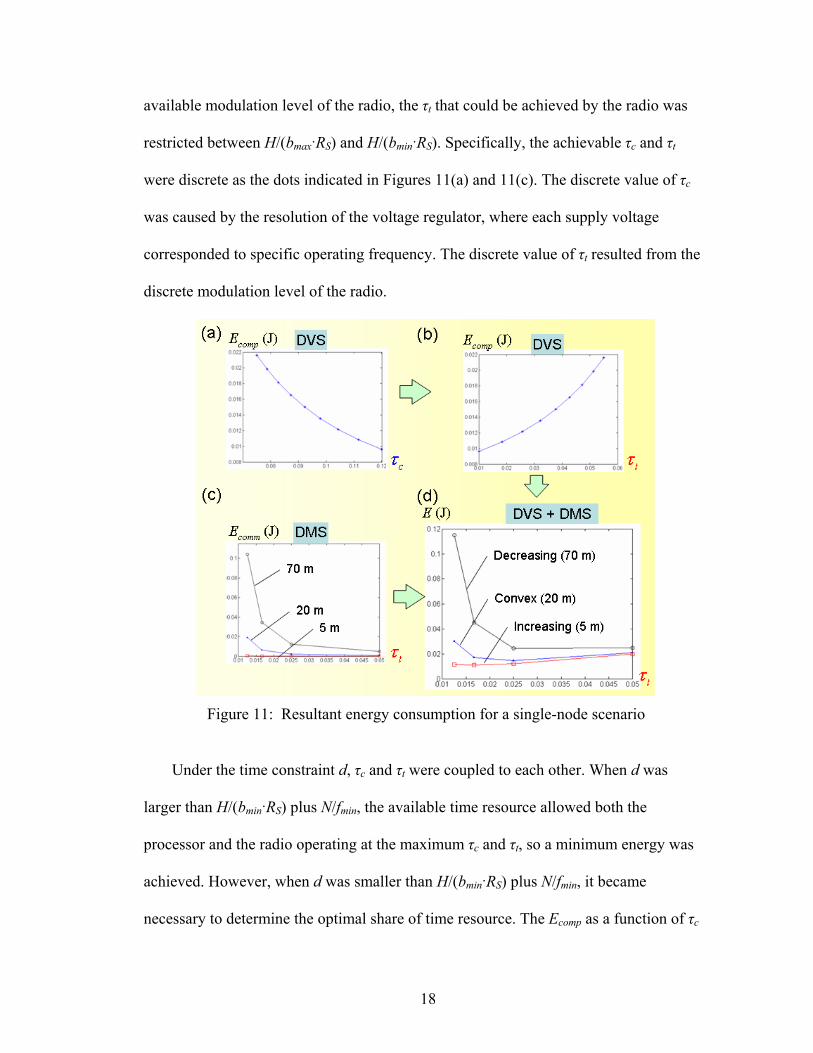
18
available modulation level of the radio, the τt that could be achieved by the radio was
restricted between H/(bmax RS) and H/(bmin RS). Specifically, the achievable τc and τt
were discrete as the dots indicated in Figures 11(a) and 11(c). The discrete value of τc
was caused by the resolution of the voltage regulator, where each supply voltage
corresponded to specific operating frequency. The discrete value of τt resulted from the
discrete modulation level of the radio.
Figure 11: Resultant energy consumption for a single-node scenario
Under the time constraint d, τc and τt were coupled to each other. When d was
larger than H/(bmin RS) plus N/fmin, the available time resource allowed both the
processor and the radio operating at the maximum τc and τt, so a minimum energy was
achieved. However, when d was smaller than H/(bmin RS) plus N/fmin, it became
necessary to determine the optimal share of time resource. The Ecomp as a function of τc

19
(= d - τt) was converted to τt as shown in Figure 11(b), so the representation of time
allocation could be indicated by a single variable τt. The reason to choose τt rather than
τc was because τt had fewer discrete values which reduced the dimension of the
optimization problem. Depending on the communication distance r, the resultant energy
consumption E (= Ecomp + Ecomm) as a function of τt exhibited three characteristics:
monotonically increasing, monotonically decreasing, and convex functions as illustrated
in Figure 11(d). The monotonically increasing function occurred in short
communication distance, where the Ecomp dominated the total energy consumption, so
the behavior of E was similar to Ecomp. The monotonically decreasing function occurred
in long communication distance, where the Ecomm dominated the total energy
consumption, so the behavior of El was close to Ecomm. As for the intermediate
communication distance, a convex function was formed due to the two comparable
energy functions, Ecomp and Ecomm. An optimization problem that minimizing the total
energy consumption in a single-node scenario was formulated as:
( )2
/( )2
min( )
(2 1)
Subject to
2,4,6,8
S t
tt
H RS t
ts
NE N CK d
F r G R
HR b
b
τ
τ ετ
τ
τ
⋅
⎛ ⎞= ⋅ ⋅ +⎜ ⎟⋅ −⎝ ⎠⎡ ⎤+ ⋅ ⋅ − + ⋅ ⋅⎣ ⎦
=⋅
=
(9)
where the solution (optimal transmission time) can be derived by solving:
( ) / 0t tdE dτ τ = (10)
( )2
2 0tt
d Edτ
τ > (11)

20
where Equation 11 proves the convexity of the energy function. Since only the sensor
node whose energy function was convex was required to solve the above optimization
problem. As for the sensor node whose energy function was monotonically decreasing
or decreasing, τt,min (= H/(bmax RS)) and τt,max (= H/(bmin RS)) could be directly
determined as the optimal transmission. By finding the critical communication distances
that distinguished the three energy function, the computational complexity in finding
the optimal transmission time was reduced. The critical communication distance was
derived by considering Equation 10 in the form of:
2 /( )1 2 (1 0.693 /( )) 0tScomp S S S t
H RE G R F R r H Rτ τ⋅⎡ ⎤′ + ⋅ − ⋅ ⋅ ⋅ − ⋅ − ⋅ =⎣ ⎦ (12)
( )
2
2
2( )
compcomp
t tt
dE N C NEd K dK d
ετ ττ
⎛ ⎞⋅′ = = +⎜ ⎟⋅ −⋅ − ⎝ ⎠ (13)
The r that satisfied Equation 12 was required to be:
/( )( )
1 2 (1 0.693 /( ))S t
comp StH R
S S t
E G Rr g
F R H Rττ
τ⋅
′ + ⋅= =
⎡ ⎤⋅ ⋅ − ⋅ − ⋅⎣ ⎦
(14)
where function g as a function of τt is a non-decreasing function. Because τt was
bounded by τt,min and τt,max, the r that satisfied Equation 14 was also bounded by g(τt,min)
and g(τt,max). Therefore, only the sensor node whose r within g(τt,min) and g(τt,max)
exhibited a convex energy function. For the sensor node whose r was smaller than
g(τt,min), dE/dτt was positive over all τt, which corresponded to the monotonically
increasing energy function. When r was larger than g(τt,max), dE/dτt was negative over
all τt, which corresponded to a monotonically decreasing energy function. This
classification technique was used to reduce the optimization complexity in the multi-
node scenario.

21
3.1.4.2 Multi-Node Scenario
The utilization of DTA in multi-node scenario was more complex since the
utilization of the available time resource depended on the chosen data acquisition
scheme and communication protocol. A real-time data acquisition was considered
where sensor nodes in the sensing field continuously monitored the environmental
phenomena and the collected data needed to be reported to the base station under the
time constraint. Unlike event-driven application where random access could be used in
the MAC (Medium Access Control) layer; such type of scenario requires channel
partitioning of the MAC layer to offer a stable network structure in sustaining
consistent data load. In this section, a data acquisition scheme and the MAC protocol
suitable for the efficient utilization of DTA is investigated, and then an optimization
problem is formulated to minimize the energy consumption of the network.
3.1.4.3 Network Sectioning
It has been investigated [5, 34] that sectioning of the WSN allowed for improved
computational efficiency in aggregating information to reduce the communication
energy. Figure 12 illustrates such cluster-based WSN, where sensor nodes are grouped
into multiple clusters with a randomly chosen cluster head in each cluster. Every cluster
head collected the extracted data from every sensor node in the same cluster and
aggregated the information (which was called data fusion) to reduce the communication
energy.

22
Figure 12: Illustration of a cluster-based WSN
3.1.4.4 Data Acquisition Scheme
Based on the cluster-based WSN, every sensor node kept sampling physical signals
and periodically extracted and transmitted the useful information to the cluster head.
The cluster head then fused all collected information and transmitted the fused data to
the remote base station. To achieve a real-time data acquisition, the time was divided
into a series of consecutive sampling period T where all the above tasks had to be
performed within each sampling period for the following tasks to be executed in time.
In addition, a parallel processing was utilized on every sensor node where raw data
were alternatively stored in a dual memory buffer, and the data collected in the previous
sampling period were processed within the current sampling period. Figure 13
illustrates a complete data acquisition scheme, which includes all the necessary tasks in
individual sampling period.

23
Figure 13: Illustration of the data acquisition scheme in a sensor network
3.1.4.5 Communication Protocol
To enable an in-cluster data communication, a reservation-based Time Division
Multiple Access (TDMA) protocol [35] was utilized to schedule the multiple access
communication. The advantage of using TDMA over FDMA (Frequency Division
Multiple Access) lied on its scalability, which allowed more sensor nodes to be
accommodated in a cluster, since only limited channel bandwidth was available for the
network. The radio circuits that implemented TDMA were simpler compared with
CDMA (Code Division Multiple Access), which resulted in lower cost of sensor nodes.
Another advantage of using TDMA was its improved energy efficiency through the
cooperation of DTA, which was described as follows.
The improved energy efficiency of using TDMA came from its data
communication structure. In the reservation-based TDMA protocol, the time was
divided into time frames as long as the sampling frame T. Each sampling frame was

24
composed of two parts: a control sub-frame and a data sub-frame as illustrated in
Figure 14. The control sub-frame was used for the exchange of control signals including
time synchronization, channel quality estimation, and the broadcasting of channel
allocation from the cluster head between the cluster head and the other sensor nodes.
Furthermore, new added sensor nodes could use the control sub-frame to join the cluster,
which increased the network scalability. The data sub-frame reserved for data
transmission was divided into time slots with variable length. The cluster head assigned
the time slots of all sensor nodes in its cluster in which every sensor node was assigned
the whole band of frequencies in a given time slot.
Figure 14: Reservation-based TDMA protocol
In the protocol, every sensor node only turned on its radio during the control sub-
frame and the assigned time slot. Such communication structure resulted in energy
savings from two aspects: first, the sensor nodes did not need to turn on the radio all the
times; second, the unused time slots before data transmission could be completely
distributed to the computation task, so DVS could exploit the time to reduce the energy
consumption. Every sensor node’s transmission time not only determined its local time
allocation among τc and τt, but also influenced other sensor nodes’ total processing time.

25
For example, when the transmission time of sensor node m, τt,m, increased 1 ms, either
the computation time of sensor node m, τc,m, or the total processing time for sensor
nodes 1 ~ m-1 had to be decreased 1 ms as well. The utilization of DTA thus had to be
considered from the whole cluster to achieve minimum energy consumption of the
network.
3.1.4.6 Solution Formulation
To achieve a DTA in multi-node scenario, an optimization problem was formulated
according to the presented data acquisition scheme and MAC protocol. The objective
function of the problem was the total energy consumption of the cluster, Etotal, and was
expressed as:
, ,1
2
/( )2
1 ,
( ) ( )
(2 1)S t
m
total comp c i comm t ii
mH R
i S ti c i
E E E
NN C F r G RK
τ
τ τ
ε ττ
=
⋅
=
⎡ ⎤= +⎣ ⎦
⎧ ⎫⎛ ⎞⎪ ⎪⎡ ⎤= ⋅ ⋅ + + ⋅ ⋅ − + ⋅ ⋅⎜ ⎟⎨ ⎬⎣ ⎦⎜ ⎟⋅⎪ ⎪⎝ ⎠⎩ ⎭
∑
∑ (15)
where the allowable computation time for sensor node i, τc,i, was calculated by:
, ,
m
c i t ij i
dτ τ=
= −∑ (16)
The symbol d referred to the time constraint, where all local computation and in-
cluster data communication had to be finished by d for the following cluster head
operation. The control variables of the objective function were converted from
transmission time τt to modulation level b, because the modulation level was the actual
control parameter of the radio. An optimization problem could be formulated as:

26
,
, ,1
/( )2 2,
1 ,
, max
, ,
( ) ( )
( ) (2 1)
1: / (Set by CPU) 2: 2,4,6,8 (Set by radio)
3: -
min
Subject to
S t i
m
total comp c i comm t ii
mH R
i S t ii c i
c i
i
mc i t ij i
E E
NN C F r G RK
C N fC b
C d
E
τ
τ τ
ε ττ
τ
τ τ
=
⋅
=
=
= +
⎡ ⎤⋅ ⋅ + + ⋅ ⋅ − + ⋅ ⋅⎣ ⎦⋅
≥
∈
=
∑
∑
,
(Set by time scheduling)
4: /( )t i S iC H R bτ = ⋅
∑
(17)
The constraint C1 was imposed by the processor capability, which indicated a
sensor node’s minimum computation time given the maximum operating frequency fmax.
The constraint C2 came from the radio limitation that only finite modulation levels were
applicable in the communication. The solution to the optimization problem was
therefore a set of modulation levels for all sensor nodes, which produced the optimal
time allocation. To solve such an integer programming problem, the exhaustive
enumeration method was only applicable for small-scale network since the
computational loads increased exponentially with respect to the sensor node numbers;
the non-linear objective function and the discrete variables precluded the use of
calculus-based optimization techniques. Thus, it became significant to derive the
optimal result efficiently for the utilization of DTA.
3.1.4.7 Dynamic Time Allocation Algorithm
A Dynamic Time Allocation (DTA) algorithm for solving the optimization problem
was developed based on the structure of the objective function and the previous
classification technique. The algorithm was implemented by the cluster head when the
network was subjected to external dynamics, such as node failure, new added node, or

27
variation in communication condition, so the time allocation could be dynamically
updated to maximize the energy efficiency.
The transmission sequence of sensor nodes in a cluster was first determined.
Considering the sensor node i used high modulation level in transmitting the data, the
total energy consumption in computation could be decreased due to the prolonged
computation time for the sensor node i and the prolonged processing times for the
sensor node 1 to sensor node i-1. Therefore, the later the transmission sequence where
the sensor node i was located, the higher energy saving could be achieved because more
sensor nodes could be benefited from the prolonged processing time. The use of high
modulation level caused an increment of communication energy of the sensor node i,
which was proportional to the communication distance between the sensor node I and
the cluster head. Hence, it was more energy efficient to schedule a sensor node with
short communication distance in the later transmission sequence, because only minor
energy overhead in communication was incurred. The transmission sequence of sensor
nodes was therefore scheduled in a decreasing order in terms of the communication
distance r, i.e., r1 ≥ r2 ≥…≥ rm.
After the determination of transmission sequence, a necessary condition for the
solution of the optimization problem (the optimal modulation level for every sensor
node) was derived stating that the modulation levels for the sensor nodes, b1, b2,…, bm,
must appear in a non-decreasing order. This statement was mathematically expressed as
Lemma 1.

28
Lemma 1: Given ri ≥ ri+1 for i = 1,…, m-1, a necessary condition for optimality of
Equation 17 was bi ≤ bi+1.
Proof: Let β be a possible solution such that bi = x, bi+1 = y, and x > y for i ∈ 1,…, m-
1. Further, suppose that β was the optimal solution of the optimization
problem. Consider another possible solution α such that bi = y, bi+1 = x, and αj
= βj for j ≠ i, i+1. Compare the value of the objective function computed from β
and α , we obtained:
( ) ( ) ( )2 2, 1 , 1 1
( ) ( )
2 1 2 1 0
total total
x y
comp i comp i i i
E E
E E H F r rx y
β α
β α+ + +
− =
⎡ ⎤− −⎡ ⎤− + ⋅ ⋅ − − >⎢ ⎥⎣ ⎦ ⎣ ⎦
(18)
The inequality contradicted the optimality of β , so the optimal solution must
abide by the condition bi ≤ bi+1.for i – 1,…, m-1.
According to Lemma 1, only the vector that satisfied the criterion b1 ≤ b2 ≤ … ≤ bm
were considered to be the possible solution. So the number of possible solutions were
drastically reduced to 11
b
b
m nnC + −− , where m was the total sensor node numbers in a cluster
and nb was the number of available modulation levels of the radio. In our case, where
four different modulation levels were available, the possible solutions were efficiently
reduced to 1 ( 3) ( 2) ( 1)6
m m m+ ⋅ + ⋅ + compared with the exhaustive enumeration, which
generated 4m possible solutions.
Furthermore, the classification technique developed in the single-node scenario was
applied to reduce the computational loads in finding the optimal solution. The concept

29
was to filter out the sensor nodes whose energy function with respect to the
transmission time were monotonically increasing or monotonically decreasing and to
assign the optimal modulation level bmax or bmin directly. The dimension of the
optimization problem could therefore be further reduced.
Since the communication distance of sensor nodes were arranged in a decreasing
order, the classification of sensor nodes with monotonically decreasing energy function
(appeared in the long communication distance) was analyzed from the sensor node 1;
the classification of sensor nodes with monotonically increasing energy function
(appeared in the short communication distance) was analyzed from the sensor node m.
The classification was performed according to Equation 14. Given specific time
constraint (d second), if a sensor node’s communication distance r was larger than
g(τt,max), the energy function of the sensor node was monotonically decreasing; if r was
smaller than g(τt,min), the energy function of the sensor node was monotonically
increasing. The critical communication distances, g(τt,min) and g(τt,max) that classified the
three energy functions varied with d as illustrated in Figure 15. The classification of a
sensor node was thus determined by a sensor node’s r and d.

30
Figure 15: Classification of sensor nodes for various communication distances and time
constraints (H = 1000 bits, N = 1.1 x 10⁸, bmin = 2, bmax = 8)
The procedure of classifying the sensor nodes with monotonically increasing
energy function was performed backward from the sensor node m. Given the
communication distance rm and the time constraint d for the sensor node m, the
classification of sensor node m as monotonically increasing energy function was
determined by its position on the classification diagram shown in Figure 15, and was
mathematically expressed as rm < g(τt,min) given time constraint d. If the sensor node m
was classified as the sensor node with monotonically increasing energy function, a
transmission time, τt,min, was assigned to the sensor node m. The procedure then
continued to classify the sensor node m – 1 with time constraint d - τt,min. The
classification continued until a sensor node was classified as the sensor node with
convex energy function.
The classification of sensor nodes with monotonically decreasing energy function
was performed from the sensor node 1. The time constraint for the sensor node 1, d1,

31
varied within d – (m-1) τt,max and d – (m-1) τt,min depending on the transmission times of
the sensor nodes 2 ~ m. If the sensor node 1 was classified as the sensor node with
monotonically decreasing energy function given the shortest possible time constraint
d – (m-1) τt,max, the sensor node 1 would have monotonically decreasing energy function
over all possible time constraints. The classification of the sensor node 1 as the sensor
nodes with monotonically decreasing energy function was then determined by r1 >
g(τt,max) given time constraint d – (m-1) τt,max. If the sensor node 1 was classified as the
sensor nodes with monotonically decreasing energy function, the procedure continued
to classify the sensor node 2 with time constraint d – (m-2) τt,max. The classification
proceeded until a sensor node was classified as the sensor node with convex energy
function.
Figure 16: Procedure of Dynamic Time Allocation algorithm
Based on the Lemma 1 and the classification technique, a DTA algorithm was
developed to find the optimal solution of the optimization problem efficiently, so the

32
cluster head could dynamically generate the optimal time allocation for the network.
Figure 16 illustrates a complete procedure of performing the DTA algorithm. First, the
cluster head acquired the communication distance from the estimation of the link
quality for every sensor node, and then scheduled the transmission sequence of sensor
nodes in a decreasing order in terms of the communication distance. The classification
technique was utilized to filter the sensor nodes with monotonically increasing energy
function and the sensor nodes monotonically decreasing energy functions. The optimal
modulation level bmax and bmin were assigned directly. For the remaining sensor nodes
whose modulation levels had not been determined, the possible solutions were reduced
according to the Lemma 1, and found the optimal solution that produced the minimal
objective function.
3.1.5 Simulation Model and Results
The energy efficiency of using DTA in the multi-node scenario was presented in
this section. A real-time machine monitoring application was considered where sensor
nodes constantly monitored the vibration signals, which were processed by using the
Discrete Harmonic Wavelet Packet Transform (DHWPT) algorithm [51] to extract the
desired information. The data processing was performed locally on the sensor nodes to
reduce the energy consumption in transmitting the raw data. The extracted data (energy
at each sub-frequency band) of every sensor node were collected by the cluster head,
and the data were fused on-line by the cluster head to diagnose the machine conditions.
The energy consumption of a single cluster was simulated on the MATLAB, where
sensor nodes were randomly deployed on a 20 x 20 m2 sensing area considering the

33
indoor transmission range of the radio. Assuming the required sampling frame was 1
second, the time reserved for the control sub-frame, data fusion, and data transmission
to the base station was 0.5 seconds, so all the tasks for local processing and in-cluster
data communication needed to be finished within 0.5 second. The processor and the
transceiver used in the simulation were Intel Xscale PXA271 [31] and the parameters of
the transceiver were derived from [36]. Table 2 lists the parameters used for the
processor and the transceiver, and the related parameters of the application.
Table 2: Parameter settings of the processor and the transceiver
Parameters Value Processor Parameters
Switching Capacitance C 1.45 nF Hardware Parameter K 870x106 MHz/V Hardware Parameter ε 0.83 V Maximum Frequency fmax 412 MHz Minimum Frequency fmin 13 MHz
Transceiver Parameters Symbol Rate RS 1.0x10⁵
symbols/second Hardware Parameter G 10 nJ/symbol Hardware Parameter F 67 pJ/symbol/m2
Application Parameters Computation task N 1.1x10⁸ cycles Communication task H 1000 bits Sampling Period T 1 second Time Constraint d 0.5 second
The effects of the dynamic time allocation on energy reduction were investigated
under different cases. In the first case, the number of sensor nodes contained in the
cluster varied with unchanged communication and computation tasks. Three different
hardware designs were considered: without hardware reconfigurability, with only DVS,
and with combined DVS and DMS. In the scheme which without using hardware
reconfigurability, the sensor nodes used fixed hardware settings, maximum operating

34
frequency fmax and minimum modulation level bmin, in processing the tasks. In the
scheme where only DVS was utilized, the operating frequency and the supply voltage
are adjustable, but only the minimum modulation level bmin was used in the
communication. In the scheme where both DVS and DMS were used simultaneously,
DTA was applied to obtain the optimal parameter settings for every sensor node. The
number of sensor nodes was simulated from 1 to mmax = 45, where mmax is the maximum
number of sensor node a cluster could accommodate when no DMS was utilized on the
sensor nodes. The value of mmax could be calculated from:
min,1 , max1
max
( )m Sc t ii
b R Nd m d mH f
τ τ=
⋅≥ − ⇒ ≥ − =∑ (19)
To evaluate the energy efficiency of the proposed node-level reconfiguration
technique, three scenarios were simulated using different level of reconfigurability as
shown in Table 3. In the first scenario, sensor nodes without DVS and DMS techniques
operated at the maximum supply voltage, maximum operating frequency, and minimum
modulation level. In the second scenario, sensor nodes only used DVS technique to
reconfigure supply voltage and operating frequency. The minimum modulation level
was used in communication. In the third scenario, sensor nodes with DMS and DVS
capabilities could reconfigure the supply voltage, operating frequency, and modulation
level.
Table 3: parameter settings for different scenarios
Scenario Voltage Frequency Modulation Scenario 1: No DVS & DMS 1.25V 416 MHz 2 Scenario 2: DVS only 0.85~1.25V 13~416 MHz 2 Scenario 3: DMS + DVS 0.85~1.25V 13~416MHz 2,4,6,8

35
In a single-node scenario, only one sensor node (Node 1) performed local
computation and transmits the data to the cluster head, as shown in Figure 17. The
minimum energy consumption was achieved by using b = 4 in the third scheme.
Figure 17: Energy consumption for a 1-node case
In a 2-node case as shown in Figure 18, there were 16 possible time allocations of
the network, where the minimum energy consumption was achieved by selecting
modulation level of Node 1, b1, equal to 4 and selecting modulation level of Node 2, b2,
equal to 6.
Figure 18: Energy consumption for a 2-node case
In a sensor network with more sensor nodes, the DTA was used to compute the
optimal modulation level for every sensor node. Figure 19 shows the energy saving
ratio for using the reconfiguration techniques (scenario 2 and scenario 3) with respect to
non-reconfigurable scheme (scenario 1), where the energy saving ratio was calculated
by:

36
with DVS (for scenario 2)
without DVS + DMSEnergy Saving Ratio = 1 - total
total
EE
(20)
with DVS + DMS (for scenario 3)
without DVS + DMSEnergy Saving Ratio = 1 - total
total
EE
(21)
Figure 19: Energy consumption for various node number and packet sizes
Figure 19 shows the energy saving for schemes 2 and 3 for various packet size (H)
and node number (m). With the increment of sensor nodes in the cluster, the average
processing time for every sensor node decreased, which increased the energy
consumption of the sensor nodes, so the energy efficiency of using DVS technique
alone decreased from 55% to 38%. By combing the DMS technique with the DVS
technique to allocate the time resource, the increment of computation energy could be
reduced by reallocating time resource from the transmission time to the computation
time. This time reallocation process increased the communication energy, but resultant
energy consumption decreased when the communication distance r was short. A 22% of
energy efficiency improvement was achieved by using DMS with DVS compared to the
scenario where only DVS was used.

37
Similar to the increasing node number, increasing the communication workload
reduced the available time for computation, so using DVS alone resulted in the decrease
of energy efficiency. With reallocation of time resource, the increased communication
time due to the increased communication workload could be shortened, thus prolonging
the computation time and correspondingly decreasing the computation energy. By
incorporating DMS with DVS, a 52% of energy savings was achieved in high
communication task, and the energy efficiency of using DMS with DMS was improved
22% compared to only the DVS technique was used.
The computation efficiency of using the developed DTA algorithm was also
investigated to estimate the computation time of finding the solution of the
optimization. The total computation time for various number of sensor nodes is shown
in Figure 20. The simulation result showed that the optimal solution could be
realistically implemented on the cluster head.
Figure 20: Computation time of the Dynamic Time Allocation algorithm

38
3.2 Network-Level Reconfiguration
Since current state-of-the-art sensor node platforms still cannot meet the demand
for high energy-efficiency, particularly in computation-intensive applications such as
image processing or vibration analysis, a WSN required a recharging service to
recharge the energy-depleted sensor nodes. The entire system could thus be called a
Rechargeable Wireless Sensor Network (RWSN). Hence, when a sensor node stopped
functioning due to discharge of the limited battery energy available, its battery could be
recharged by the recharging service to restore the sensor node to a functional level.
To realize a functional RWSN, the associated maintenance cost needed to be
minimized as it ultimately determined the acceptability of the RWSN. The cost was
related to the recharging rate (the number of recharging energy-depleted sensor nodes
per unit time), which must be minimized. Intelligent node activation was an approach to
achieving this objective by dynamically controlling node activities to conserve energy
at the sensor node level. It involved redundant deployment of sensor nodes to allow a
sensor node to go into sleep mode without degrading network performance. This
reduced the overall energy consumption of the network by taking redundant nodes off
line and scheduling active/sleep states of the sensor nodes [37].
Traditional scheduling algorithms based on a battery-powered scenario were not
suitable for RWSN because these algorithms did not consider the scenario of recharging
the sensor nodes. Thus, a new algorithm was required for solving the node activation
problem of a RWSN. A major challenge in developing such an algorithm was to tackle
the dynamic discharging and recharging processes during the network operation. A
dynamic discharging process was necessitated by the random occurrence of events of

39
interest, which affected the energy consumption in data processing and data
communication. The random occurrence of objects in a surveillance sensor network that
resulted in the temporal and spatial variation of energy consumption of sensor nodes
was one such event. An unpredictable recharging service, where the waiting time for the
energy-deployed sensor nodes varied depending on the progress of the recharging
service was another. Such applications motivated the development of an analytical
framework that captured the stochastic nature of RWSN network operations.
In the following sections, the background of RWSN and related research was first
presented. Mathematical formulation of the problem was then developed. Finally, the
effectiveness of the developed algorithm was demonstrated.
3.2.1 Background
The realization of a RWSN was tied to the recharging service to sustain the
network operation. When the battery voltage of a sensor node dropped below a
threshold level due to the sensing operation and data communications, the sensor node
stopped the sensing operation and transitions from the active state to the passive state,
waiting for the recharging service. After recharging for a time until the completion of
the recharging service, the sensor node went into the ready state and could be activated
at any time to rejoin the network operation. Thus, every sensor node in a RWSN
operated among the three node states as shown in Figure 21, and ideally, the network
should be able to operate continually as long as the recharging service was functional.

40
Figure 21: Three node states of sensor nodes in RWSN
The network performance of a RWSN, such as area coverage, network connectivity,
or network detectability of a moving target, was determined by the number of sensor
nodes in the active state, which varied with time due to the stochastic discharging and
recharging time. Sufficient recharging service had to be provided in order to achieve the
required time-average network performance. In this paper, area coverage, the fraction
of the geographical area covered by one or more sensor nodes, was used as the
performance metric of the network since it was widely used in WSN [38, 39]. However,
the other network performances cold also be applied by changing the utility function.
Assuming every sensor node had a disk shaped sensing area with same sensing range r,
a sensor node could only detect events that happened within its sensing range.
Assuming sensor nodes were distributed uniformly and independently in the sensor
field [39], the utility function for calculating area coverage U was:
2( ) 1 d rU d e τ− ⋅ ⋅= − (22)
where d is the active node density (number of active sensor nodes per unit area) and the
time-average area coverage U was:

41
0
1lim ( ) t
tU U d dt
t→∞= ∫ (23)
The area coverage as a function of d was a monotonically increasing concave
function as shown in Figure 22. The purpose of intelligent node activation was to
influence the distribution of d with respect to time by a sequence of activation decisions,
so the time-average area coverage could be maximized.
Figure 22: Recharging scheme and area coverage w.r.t. active node density (r = 7 m)
However, over-activation of sensor nodes increased a short-term marginal
increment of area coverage but lead to less active sensor nodes in a later time, which
resulted in a poor time-average area coverage. Conversely, under-activation directly
resulted in poor area coverage. Deriving an activation policy to prevent over-activation
or under-activation was the critical problem for the efficient use of RWSN.
3.2.2 Literature Review
The scenario of RWSN could represent traditional maintenance service, where the
energy-depleted sensor nodes were recharged by technicians. The RWSN could also
represent several scenarios for inaccessible WSNs, where the recharging services were
used to sustain the network operation. For instance, in [40], one or multiple mobile
robots were placed in the sensor field. These mobile robots could move to the location

42
of every sensor node to recharge the sensor nodes through inductive coupling or direct
electrical connection. In [41, 42], some mobile sensor nodes with energy-harvesting
capability could deliver energy to the stationary sensor nodes to perform the recharging
service. Intelligent node activation for these RWSN scenarios was important in
reducing the burden of the recharging service.
The node activation problem for RWSN was first addressed by Kar in 2005 [43]. In
this paper, a simple Threshold Activation Policy (TAP) was proposed instead of directly
formulating a stochastic decision process. In the TAP algorithm, by assigning a
parameter s, a ready node was activated only when the number of active nodes is below
s; otherwise, the node stayed at the ready state until any active node depletes its energy.
The advantage of using TAP was that the network operation could be modeled as a
closed queueing network, and the static analysis approach for a queuing model could be
used to derive the optimal threshold value. In [44], the problem was modeled as a
closed two queue system where the node activation was derived by the optimal control
of admission to a station. However, a mathematical model based on the stochastic
decision process was required to gain an insight into the node activation problem and
provide an analytical framework for further related problems.
The operation of the rechargeable sensor network utilizing the TAP algorithm is
illustrated in Figure 23, there were two stations in tandem in the queueing network. The
first station represented the discharging process in which at most s active nodes were
allowed to stay; otherwise, the remaining nodes had to queue in the ready state. The
second station represented the recharging process with infinite capacity. The nodes in
the active state drained out their energy reserve immediately enter this station waiting

43
for recharging service. After the recharging service, the nodes returned the first station
and repeated the same cycle.
Figure 23: Queueing network model
Under the assumption of exponentially distributed discharging time and recharging
time with means μd-1 and μr
-1, the analysis approach for queueing model could be used
to derive the equilibrium probability of the model. The analysis was preceded in the
following way. First, depending on the number of nodes in the two stations, the system
could be defined in the state of (n1, n2), where n1 was the number of nodes in the first
station and n2 was the number of nodes in the second station. For the independent
sensor lifetime where discharging and recharging times of all nodes were mutually
independent, when n1 = j, the arrival rate of the first station, μj, could be expressed as:
( ) , = 0,1,...,j rn j j nμ μ= − ⋅ (24)
The departure rate of the first station, λj, was expressed as:
, = 1,2,...,
, = +1, +2,...,d
jd
j j ss j s s nμ
λμ⋅⎧
= ⎨ ⋅⎩ (25)
Based on Equations 24 and 25, the relation between system states are illustrated in
Figure 24. In the figure, each circle represented the system state (n1 = j, n2 = n - j). The
arrows connecting two system states were the transition rate between states. The dotted

44
line separated the system states into the condition that no ready nodes queued in the
first station (left side) and ready nodes queued in the first station (right side).
Figure 24: Transition process of the queueing model
The equilibrium probabilities for system state (n1 = j, n2 = n - j), Pj, could be
derived from a set of balance equations as shown in Table 4.
Table 4: Balance equations of the queueing model
System State Flow-Out = Flow-In j = 0 P0 n μr = P1 μd
1 ≤ j ≤ s-1 Pj [(n - j) μr + j μd] = Pj-1 (n – j + 1) μr + Pj+1 (j + 1) μd j = s Ps [(n - s) μr + s μd] = Ps-1 (n – s + 1) μr + Ps+1 s μd
s+1 ≤ j ≤ n-1 Pj [(n - j) μr + s μd] = Pj-1 (n – j + 1) μr + Pj+1 s μd j = n Pn s μd = Pn-1 μr
By introducing the normalized condition, 0
( ) 1njj
P n=
=∑ , the equilibrium probability for
each system state could be obtained as:
( )
0
0
, = 1,2,..., -1
! , = , +1,...,! !
j
jj
j s
na P j s
jP
n a P j s s nn j s s −
⎧ ⎛ ⎞⎪ ⎜ ⎟⎪ ⎝ ⎠= ⎨⎪⎪ −⎩
(26)
where a = μr / μd and P0 is given by:
-11
0k=0
!( )! !
s nk k
k sk s
n nP a ak n k s s
−
−=
⎡ ⎤⎛ ⎞= +⎢ ⎥⎜ ⎟ −⎝ ⎠⎣ ⎦∑ ∑ (27)
The time-average area coverage, U , was thus calculated from:

45
1 1( ) ( )s n
j jj j sU U j P U s P
= = += ⋅ + ⋅∑ ∑ (28)
By selecting appropriate threshold value, s, that maximizes U , a near-optimal time-
average area coverage could be obtained. As for the correlated sensor lifetime where
the discharging (recharging) times of all nodes entering the active (passive) state at the
same time was the same, the time-average area coverage could also be derived by using
a variant of the queueing model. Figure 25 illustrates the results computed from the
threshold activation policy for the independent and correlated sensor lifetime.
Figure 25: Time-average area coverage for threshold activation policy [43]
The theoretically upper bound of U was 1( )
1nUa−+
and the threshold activation
policy was proved to achieve at least ¾ of the theoretical upper bound [43]. The simple
characteristic of TAP algorithm made it easy to be implemented on nodes, and the
algorithm required the nodes only to keep track of the node states in its immediate
neighborhood.

46
3.2.3 Semi-Markov Decision Process
The main contribution of this technique was the mathematical formulation of the
intelligent node activation problem. Two assumptions were made in the model for
analytical tractability.
(1) Markovian property: The future network state depended only upon the present
state and the selected activation decision, without influence by the previous history.
This was an important simplifying assumption, which reduced the complexity of
planning decisions.
(2) Exponential distribution of service time: The discharging and recharging times
of any sensor node were assumed exponentially distributed with means μd-1 and μr
-1.
The exponential distribution enabled the occurrence of the event to exhibit the Markov
property, so the remaining time to the next event was always independent of the
previous elapsed time.
The optimal activation decisions under these assumptions depended only on the
number of sensor nodes in different node states. Without the assumptions, the network
operation would be very difficult to analyze, and required more exchange of network
information at the cost of increased communication overhead. Under the two
assumptions, the operation of a RWSN could be cast as a Semi-Markov Decision
Process (SMDP). The optimal activation decisions could be analytically derived by
building the model for SMDP.

47
3.2.3.1 Model Definition
Some basic terms of the SMDP related to the problem were first defined. The
network state, which was used to represent the network status, was defined as the
distribution of sensor nodes in the three node states. The network state was denoted as si
= (nr, na, np), where nr, na, and np were the number of sensor nodes in ready, active, and
passive state. The sum of nr, na, and np was equal to the total number of sensor nodes, n.
Accordingly, there were (n+1) (n+2)/2 states for an n-node sensor network. For
example, a 3-node sensor network had 10 network states, which are listed in Table 5.
Table 5: Network States for a 3-node Sensor Network
States nr na np s1 0 0 3 s2 0 1 2 s3 0 2 1 s4 0 3 0 s5 1 0 2 s6 1 1 1 s7 1 2 0 s8 2 0 1 s9 2 1 0 s10 3 0 0
The action represented the activation decision at each network state in our problem.
The purpose of taking actions in a decision process was to influence the proceeding
network states in order to maximize the time-average area coverage. The actions were
denoted as am, where m represented the number of ready nodes being activated at a
specific network state. For network state si = (nr, na, np), m could be a value between 0
and nr. The policy, denoted as φ, determines the action chosen in every network state.
The policy for a network with x network states was a x-tuple. Each element of the x-
tuple specified the action to be selected in each network state according to the policy φ.

48
For a 3-node sensor network, when the policy φ = (a0, a0, a0, a1, a0, a1, a0, a1, a2, a2)
was adopted, no node would be activated in network states s1, s2, s3, s5, s7, only one
node would be activated in network states s4, s6, s8, and two nodes would be activated in
network states s9, s10.
3.2.3.2 Transition Properties
When an action was selected in a network state, the network undergone a transition
process with specific duration (transition time), area coverage (transition reward), and
then jumped to another network state with specific probability (transition probability).
These transition properties constituted the theoretical model of a SMDP problem, so it
was critical to model the transition process for the derivation of these transition
properties. When action am was adopted in network state si = (nr, na, np), the network
immediately changed to an intermediate network state si’ = (nr-m, na+m, np) and started
a transition process as shown in Figure 26.
Figure 26: The network state, selected action, and sequential transition process
Under the assumption of the exponential distribution of the mean discharging rate
μd and mean recharging rate μr, the resultant discharging rate of active nodes entering

49
the passive state was (na+m) μd, and the resultant recharging rate of passive nodes
entering the ready state was np μr. Primarily, these two events caused the network to
change state and terminate the transition process. When an active node entered the
passive state, the network jumped from the intermediate network state si’ to state sj =
(nr-m, na+m-1, np+1); when a passive node entered the ready state, the network jumped
from the intermediate network state si’ to network state sj = (nr-m+1, na+m, np-1).
Assuming the possibility that multiple events happened at the same time was negligible,
sj could only be the above two network states. The transition properties for each
network state-action pair were thus computed based on this transition process.
Transition probability, p(si, am, sj), was the probability that the network jumped to
the next network state sj when action am was selected at the current network state si. The
sj could only be (nr-m, na+m-1, np+1) and (nr+1, na, np-1) depending on which event
happens first in the network: an active node entering the passive state or a passive node
entering the ready state. The transition probability to these two network states were the
fraction of the resultant discharging rate or the resultant recharging rate to the sum of
the two resultant rates, and the transition probabilities to the other network states were
zero. Equation 29 mathematically expressed the transition probabilities for all network
states as:
( , , )
( )for ( , 1, 1)
( )
for ( 1, , 1)( )
0 for other networkstates
i m j
a dj r a p
p r a d
p rj r a p
p r a d
p s a s
n ms n m n m n
n n m
ns n m n m n
n n m
μμ μ
μμ μ
=
+ ⋅⎧ = − + − +⎪ ⋅ + + ⋅⎪⎪ ⋅⎪ = − + + −⎨
⋅ + + ⋅⎪⎪⎪⎪⎩
(29)

50
The derivation of Equation 29 was as follows. We denoted E = Ea to represent the
event that an active node first entered the passive state within the transition process and
E = Ep represented the event that a passive node first entered the ready state during the
transition process. Assuming U = minEa, Ep, the probability that E = Ea and U > t
was equal to:
( )
( )
(( ) )
(( )
Pr , Pr
( )
( )
( )(( ) )
( )
( )( )
a p
a a p
a d p rt x x
a d at
a da d p r a
a d p r t
a d
a d p r
n m x n xa a p r pd
n m xn x a ap r a d
n m n xa p r ad
n m na pd
E E U t t E E
n m e n e
e n m e dx
n mn m n e dx
n m n
n me
n m n
μ μ
μμ
μ μ
μ
μ μ
μ
μμ μ
μ μ
μμ μ
< <
∞
∞
− + −
− +−
− + +
− + +
= > = < <
= +
= +
+= + +
+ +
+=
+ +
∫∫
∫
∫)trμ
(30)
The transition probability p(si, am, sj) for sj = (nr-m, na+m-1, np+1) was:
( )Pr Pr , 0
( )a d
a aa d p r
n mE E E E U
n m nμ
μ μ+
= = = > =+ +
(31)
The transition probability p(si, am, sj) for sj = (nr+1, na, np-1) was:
Pr 1 Pr ( )
p rp a
a d p r
nE E E E
n m nμμ μ
= = − = =+ +
(32)
Transition time, t(si, am, sj), was the duration from the current network state si to the
next network state sj given action am was chosen at si. Since the transition time was a
random variable due to the stochastic discharging and recharging process, the value of
the transition time was determined by the expected value of t(si, am, sj). Because the
resultant recharging time and resultant discharging time were distributed exponentially

51
with means of (np μr)-1 and ((na+m) μd)-1, the probability that the network changed the
network state at time t was calculated as:
(( ) )
( | , )
(( ) )
i m
a d p r
n m n ta p rd
f t s a
n m n eμ μ
μ μ− + ⋅ + ⋅ ⋅
= + ⋅ + ⋅ ⋅ (33)
To derive the probability density function, f(t | si, am), we first obtained the
cumulative distribution function via
(( ) )
(( ) )
1 Pr 1 Pr , Pr ,
( )1
( ) ( )
1
a p
p ra d
a d p r a d p r
n m n ta p rd
n m n ta p rd
U t E E U t E E U t
nn me
n m n n m n
e
μ μ
μ μ
μμμ μ μ μ
− + +
− + +
− > = − = > − = >
⎛ ⎞+= − +⎜ ⎟⎜ ⎟+ + + +⎝ ⎠
= −
(34)
The probability density function (Equation 33) could then be derived by taking the
first derivative of the above cumulative distribution function.
The expected value of t(si, am, sj) over all network states was calculated as:
0
( , , )
1( | , )( )
i m j
i ma d p r
t s a s
t f t s a dtn m nμ μ
∞= ⋅ =
+ ⋅ + ⋅∫ (35)
Transition reward represented the area coverage in our case since area coverage
was used as the performance metric of the network. According to Equation 23, the
value of the area coverage was expressed as:
2( / ) 1a
d rU d N A e π− ⋅ ⋅= = − (36)
where A is the total area of the sensor field and Na is the number of active nodes. The
transition reward, r(si, am, sj), represented the area coverage in the transition process
when the network was going from network state si to sj under the influence of action am.
Because the system stayed at the intermediate network state during the whole transition

52
process, the transition reward was completely governed by the active node numbers in
the intermediate network state, and was calculated as:
( , , ) ( )ai m j
n mr s a s UA+
= (37)
In the next section, the derived transition properties were embedded into the SMDP
model to obtain the optimal policy that maximized the time-average area coverage.
3.2.3.3 Solution Formulation
The objective of formulating the SMDP was to find the optimal policy, φ*, which
maximized the time-average reward (area coverage) as expressed by:
0
1lim ( ) t
xtE U d dx
t =→∞
⎡ ⎤⎢ ⎥⎣ ⎦∫ (38)
where d is the active node density that varies with time. This average utility problem
could be solved by using the discounted utility problem as the discounted factor, e-a x,
approached unity. Specifically, considered the problem of maximizing:
0lim ( )
t x
xtE e U d dxα− ⋅
=→∞
⎡ ⎤⋅⎢ ⎥⎣ ⎦∫ (39)
where α is the discounting coefficient. The policy that optimized the total discounted
reward in Equation 39 is also the optimal policy for the problem of Equation 38 when
the discounted coefficient α approached zero [45]. The policies for SMDP were
evaluated with respect to this expected total discounted reward in order to avoid an
unbounded value function problem when using the Bellman equation. The Bellman
equation used the recurrent relationship of state to yield optimal solutions to SMDP
problems. In the Bellman equation, associated with every network state, there existed a
scalar quantity for a given policy. Each scalar quantity, called a value function, was the

53
expected total discounted reward starting from a given network state along the infinite
time trajectory. These quantities formed a value function vector, which needed to be
maximized by choosing an optimal policy.
The basic recurrence concept of the Bellman equation was illustrated in Figure 27
[46, 47], where Jφ(si) denotes the value function of state si under policy φ. Assuming the
next network state was sj, the transition time t(si, φ(si), sj) and the transition reward r(si,
φ(si), sj) could be calculated from the previous section. According to the definition of
the value function, Jφ(si) was equal to the total discounted reward earned during the
one-step transition from si to sj plus the value function of the network state sj. Such a
recurrence relationship was mathematically expressed as:
( , ( ), )( ) ( , ( ), ) ( )i i jt s s si i i j jJ s R s s s e J sα ϕ
ϕ ϕϕ − ⋅= + ⋅ (40)
where R(si, φ(si), sj) is the total discounted reward earned during the one-step transition
process. The value of R(si, φ(si), sj) was the expected value of the total discounted
reward, which was calculated from:
0 0
( , ( ), )
[ ( , ( ), ) ] ( | , ( ))
i i j
x ti i j i ix t
R s s s
e r s s s dt f x s s dxα
ϕ
ϕ ϕ∞ − ⋅
= == ⋅∫ ∫
(41)
Figure 27: Recurrence relation of the network states and associated value functions

54
If the action specified by the policy φ at state si, φ(si), was am, then Equation 41
could be further simplified to:
( , ( ), )( , ( ), )
( )i i j
i i ja d p r
r s s sR s s s
n m n
ϕϕ
α μ μ=
⎡ ⎤+ + ⋅ + ⋅⎣ ⎦ (42)
Furthermore, since sj could be any state, the expectation of Jφ(si) over all network
states was used in Equation 40 by introducing the transition probability p(si, φ(si), sj):
( , ( ), )
( , ( ), )
( )
( , ( ), )[ ( , ( ), ) ( )]
( , ( )) ( , ( ), ) ( )
j
j
i
i i j i i j js S
i i i i j js S
t s s si i j
t s s si i j
J s
p s s s R s s s e J s
R s s p s s s e J s
ϕ
ϕ
ϕ
α ϕ
α ϕ
ϕ ϕ
ϕ ϕ
∈
∈
− ⋅
− ⋅
= + ⋅
= + ⋅ ⋅
∑
∑
(43)
where R(si, φ(si)) is the expected value of R(si, φ(si), sj) over the set of all network states,
S. Equation 43 was the final form of the Bellman equation for one of the network states.
The Bellman equation was therefore a system of linear equations in which the
unknowns were the elements of the value function associated with the given policy.
By solving the Bellman equation, the value function vector associated with a given
policy was obtained. The optimal policy was found by enumerating every possible
policy and choosing the policy that produces the maximum value function. However,
such an exhaustive enumeration was not an attractive proposition from the
computational point of view. Hence, the value iteration method, a computation-efficient
algorithm, was utilized in our study to solve the Bellman equation.
3.2.3.4 Value Iteration Algorithm
The value iteration algorithm was chosen to compute the optimal policy due to its
computation efficiency and simple program structure. The value iteration algorithm

55
used the Bellman optimality equation, which was modified from the Bellman equation,
to avoid the necessity of solving the system of equations. The Bellman optimality
equation used for the value iteration was expressed as:
*
*
( )
( , , )
( )
max [ ( , ) ( , , ) ( )]m i
j
i
i m i m j ja A s s S
t s a smi j
J s
R s a e p s a s J sα
∈ ∈
− ⋅= + ⋅ ⋅∑ (44)
where A(si) is the set of available actions in network state si and J* terms are the optimal
value functions computed from the optimal policy. The algorithm needed for solving
the Bellman optimality equation was given below:
Step 1: Set k = 1 and select an arbitrary vector J1. Specify ε > 0.
Step 2: For each si ∈ S, compute Equation 45, i.e., find the action that maximizes the
updated value function:
( )
1
( , , )
( )
max [ ( , ) ( , , ) ( )]m i
j
i
i m i m j ja A s s S
k
t s a smi j k
J s
R s a e p s a s J sα
∈∈
+
− ⋅
←
+ ⋅ ⋅∑ (45)
Step 3: If 1( )k kspan J J ε+ − < (which will be discussed later) go to Step 4; Otherwise
increase k by 1 and go back to Step 2.
Step 4: For each si ∈ S, choose the ε-optimal policy, β, according to Equation 46 and
stop.
( )
( , , )
( )
arg max [ ( , ) ( , , ) ( )]m i
j
i
i m i m j ja A s s S
t s a smi j k
s
R s a e p s a s J sα
β
∈∈
− ⋅
∈
+ ⋅ ⋅∑ (46)
The value iteration algorithm initiated from a random selected value function
vector J1. During the iteration k, the Bellman optimality equation in Step 2 produced an
updated value function vector Jk+1 and an improved policy dk+1 by selecting the action

56
am that maximized the value function. As the iteration number increased, the obtained
policy d approached the optimal policy and the value function converged to the optimal
value function. The termination mechanism in Step 3 used the span [48]. Given a vector
x , the span of x is defined as:
( ) max ( ) min ( )ii
span x x i x i= − (47)
With the increment of the iteration number, the span of the difference vector (Jk+1 -
Jk) kept getting smaller. The parameter ε was used to set the stopping criteria. The
iteration terminated when the span of the difference vector for two consecutive value
function vectors was smaller than ε. Hence, for a given positive value of ε, the
algorithm terminated in a finite number of steps. At the end of the algorithm, a near-
optimal policy could be produced which tries to maximize the time-average area
coverage of the network. The smaller the value of ε, the closer the obtained policies
were to the optimal policy, but it also resulted in a longer computational time to
produce the near-optimal policy.
The SMDP algorithm for intelligent node activation was based on a centralized
scheme, where a central sensor node kept track of every sensor node’s status and
determined the activation of ready nodes according to the optimal policy. Since the
sensor nodes changed their node states only when they deplete their energy or finish
recharging, a constant information exchange between the network nodes could be
avoided. This minimized the communication energy overhead. A simulation of the
intelligent node activation was conducted to test the effectiveness of the proposed
SMDP algorithm.

57
3.2.4 Simulation Model and Results
A surveillance application was used to evaluate the SMDP algorithm. Area
coverage was an important performance metric for a surveillance system. The sensor
nodes were assumed to be deployed uniformly and independently on a sensor field with
node density dn = 0.04 nodes/m2. This was the node density used by warehouse or
residential monitoring scenarios. Every sensor node was equipped with multiple sensors
to increase the capability in classifying the targets. A magnetometer, an infrared sensor,
and an acoustic sensor with sensing ranges of 7, 12, and 50 m, respectively were
included [49]. The sensing range for every sensor node was assumed to be 7 m, which
was the shortest sensing range of the three sensors. Two different correlation models for
the sensor nodes were considered:
Independent sensor model: The discharging and recharging times of all sensor
nodes were mutually independent.
Correlated sensor model: The sensor nodes entered the active (passive) state at the
same time and had the same discharging (recharging) time; otherwise, the discharging
and recharging times of the sensor nodes were mutually independent to each other.
The two sensor models were used to represent different realistic RWSN
environments. If the local computation and the resulting data transmission was the
major energy expenditure of a sensor node, the discharging times were better
represented by the independent model since the events were assumed to occur randomly
in the sensor field. On the other hand, in the rare event application, when the sensing
activity was the major source of energy consumption, the discharging times were better
modeled by the correlated model. Similarly, the recharging time was better represented

58
by the independent model when the recharging service was provided individually and
by the correlated model when the recharging service could recharge multiple sensor
nodes at the same time.
The effectiveness of the SMDP algorithm was compared with the theoretical upper
bound of time-average area coverage and with the scenario where no activation
algorithm was used. The theoretically upper bound for a specific recharging and
discharging rate was calculated by [43]:
( )1 /
nupper
d r
dU U
μ μ=
+ (48)
The scenario without using an activation algorithm suggested that the sensor nodes
leaving the passive state were activated immediately. The simulation was conducted to
acquire the necessary recharging-to-discharging ratio (μr/μd) for various time-average
area coverage requirements. Under a specific time-average area coverage requirement, a
lower recharging-to-discharging ratio suggested that a lower recharging service was
required for the RWSN.
Figure 28 illustrates the results for the independent sensor model. The time-average
area coverage with and without using intelligent node activation appeared to be close to
each other and the results for both cases were close to the upper-bounded value. This
was because the distribution of the sensor nodes entering the active state was evenly
distributed in the independent sensor model. The situation of over-activation did not
happen during this network operation, thus good energy efficiency was achieved with
and without the intelligent node activation.

59
Figure 28: Network performance for the independent sensor model
However, when the sensor model was highly correlated as shown in Figure 29,
over-activation of sensor nodes occurred when intelligent node activation was not used.
The required recharging-to-discharging ratio had to be increased in order to meet the
required time-average area coverage. The utilization of the proposed SMDP
significantly reduced the demand for recharging service. For various time-average area
coverage requirements, up to 72% of recharging rate was achieved by using SMDP
algorithm compared to no activation algorithm was used. The reduced recharging rate
greatly decreases the cost, in terms of capital, of maintaining the network.

60
Figure 29: Network performance for the correlated sensor model
In realistic applications, such as surveillance systems or machine monitoring
applications, the sensor models tended to be highly correlated because the sensor nodes
in the near sensor field had similar probabilities of detecting the same events, and
consumed energy at the same rate for the resulting data processing and the data
communication operations. The sensor nodes were recharged at the same time very
close in time because the recharging services of the sensor nodes were scheduled in a
batch due to their geographical proximity. The proposed SMDP algorithm, which
performed well in the correlated sensor models, should achieve high energy-efficiency
in these applications.

61
3.3 Implementation
This section presents an implementation for the previously proposed energy-
efficient data acquisition scheme that enables continued data sampling and on-node data
feature extraction, based on the DVS concept. A reservation-based Time Division
Multiple Access protocol was employed to allow staggered data transmissions within a
sensor cluster. As a result, sensor nodes that were scheduled to transmit their data later
in the sequential order could take advantage of the “extra” time allocated to slow down
the speed of data processing by lowering the supply voltage, thereby reducing energy
consumption. The design of reconfigurable sensor nodes was demonstrated through the
integration of a Crossbow Imote2 platform with a customized sensor board. The Imote2
utilized an Intel XScale PXA271 processor with DVS capability. The sensor board,
containing a sensor interface and an A/D converter, was designed for high sampling rate
applications enabled by Direct Memory Access (DMA) through the Serial Peripheral
Interface of the CPU, As a result, concurrent processing of signal sampling and local
data computation were achieved for real-time applications.
To evaluate the developed data acquisition scheme, a sensor network was designed
that featured autonomous sensor cluster head selection, time synchronization, and
dynamic allocation of computation times at the sensor node level. Its performance was
comparatively evaluated against a conventional sensor network that employed
maximum operating frequency for task execution and transmission using the Carrier
Sense Multiple Access (CSMA) protocol. Energy models for these two comparative
scenarios were first developed, and simulation results were compared experimentally. It
was found that energy reduction of up to 50% could be achieved using the

62
reconfiguration sensor hardware, which effectively translated into prolonged service life
for the sensor network.
3.3.1 Network Operation
A self-configuring sensor network system was developed to realize the proposed
data acquisition scheme. Figure 30 illustrates the network operation for the
implementation of the reconfigurable sensor network.
Figure 30: Network initialization and formation
The sensor network was initiated when receiving a request from the base station. At
first, a mesh network was formed to select a cluster head (CH). The selected CH then
performed time synchronization to align the sampling frames, so every sensor node
could perform computation and communication tasks as scheduled in the data
acquisition scheme. Afterwards, the CH performed dynamic time allocation to calculate
the computation and transmission time (τt and τc) for every sensor node. A sensor
network with start topology was then created to begin the data acquisition process.

63
Because the CH consumed the most energy due to the extra data fusion and data
communication, the selection of CH had to be performed periodically in order to
distribute the workload to the sensor nodes. The following subsections introduce the
important technique and algorithm used in the network operation.
3.3.1.1 Cluster Head Selection Algorithm
A distributed algorithm run on individual sensor node without the coordination of a
central control unit was developed to select the CH. Unlike the algorithm proposed in
[70] that sensor nodes self-elected themselves as a CH with equal probability, the
energy level of sensor nodes were considered in our algorithm to select the sensor nodes
with higher remaining battery energy as the CH. In the selection mechanism, an energy
level index ℜ (0~1) related to the current battery voltage output Vbatt was defined as:
max
batt th
th
V VV V
−ℜ =
− (49)
where Vth is the minimum battery voltage that can support a normal operation of sensor
nodes and Vmax it the maximum battery voltage. In the CH selection process, a sensor
node self-elected itself as a CH in several attempts r according to the probability Pelect:
( , ) ( ) ( )electx rP r w e y z η− ⋅ℜ = ⋅ + ⋅ ⋅ℜ + (50)
where w, x, y, and η are coefficients. Pelect as a function of r and ℜ increased with ℜ,
but decreased with r. The use of r prevented the sensor nodes with high remaining
energy from continuously competing to each other, which prolonged the total CH
selection process. In the CH selection process, at least one attempt (r = 1) was
performed by every sensor node to elect itself as a CH according to respective Pelect(r=1,

64
ℜ). If a sensor node self-elected itself as the CH, it broadcasted a CH announcement,
and waited for a period tCH. If no other sensor nodes also broadcasted the CH
announcement within tCH, the sensor node was selected as the CH; otherwise, the sensor
node entered the second attempt (r = 2) with a lower self-election probability Pelect(r=2,
ℜ). A sensor node declared itself as a normal sensor node when it failed in the self-
election and heard the CH announcement from other sensor nodes. If a sensor node
failed at the self-election but without hearing any CH announcement within tCH (no
sensor node was self-elected as the CH), the sensor node still went to the next attempt
and continued to self-election process. The CH selection process lasted until only one
sensor node was self-elected as the CH.
Figure 31: Cluster head selection process
Figure 31 demonstrates the above CH selection process using five sensor nodes
(Node 1 ~ Node 5) with different battery energy. In the first attempt of self-election for
all sensor nodes, Nodes 2 and 4 with lower Pelect failed in the self-election process. They
classified themselves as normal sensor nodes (withdraw from the CH selection process)
when they heard the CH announcements broadcasted by Nodes 1, 3, and 5. Nodes 1, 3,

65
and 5 participated in the second attempt of self-election process. Because no any sensor
node succeeded at the self-election process, they all stepped into the third attempt of
self-election process in which only Node 5 succeeded in the self-election process. After
tCh, Node 5 declared itself as the CH, which ended the CH selection process.
Consequently, the sensor node with high energy could be selected as CH without
exchanging all energy information among the cluster.
3.3.1.2 Time Synchronization Protocol
The time synchronization was used in network operation to unify the timer of every
sensor node to the timer of CH (global timer). A Flooding Time Synchronization
Protocol (FTSP) [50] was adopted that used a single broadcasted message to obtain time
synchronization between CH and the other sensor nodes. The FTSP achieved time
synchronization utilizing a single radio message time-stamped at both the sender and
receiver sides. The broadcasted message contained the 8-byte time-stamped information
of the CH. The sensor nodes recorded the local time while receiving the message.
Therefore, one broadcast message provided synchronization information (global timer,
local timer) for all sensor nodes.
Figure 32: Time synchronization message over the radio

66
The time synchronization message started with the transmission of preamble bytes,
followed by start of frame delimiter field (SFD), followed by the time-stamped data and
data used for the estimation of channel condition, and finally ended with CRC bytes.
The timer of the CH (T1) and sensor nodes (T2) were stamped at the end of SFD field.
There was a time elapsed between transmission of SFD field and reception of SFD field
due to the over-the-air propagation and radio hardware propagation. The message
layout was illustrated in Figure 32. Since RF propagation time was small in the short-
range transmission, its effect could be ignored. The hardware propagation delay was
empirically determined. Using T1, T2, and determined propagation delay, the time
offset between the global timer and local timer could be calculated by T1 – T2 + delay,
so the global timer (= local timer + time offset) were available for every sensor node.
The time synchronization was first performed by intensively sending 20
synchronization messages at the initialization stage for fast timer convergence. After
that, one time synchronization message was broadcasted at every control sub-frame to
rectify the error caused by slightly different frequencies of 13MHz crystal oscillators on
sensor nodes for maintaining the synchronization accuracy. The experimental results in
[50] showed that the error from such repetitive re-synchronization was below one
microsecond, which was precise for sampling frame alignment and the staggered
transmission.
3.3.1.3 Dynamic Time Allocation
After the initialization phase (CH selection and time synchronization), the CH
determined the sensor node transmission sequence in the data acquisition scheme. The

67
sensor nodes with higher remaining energy were scheduled at the former sequence to
average the remaining energy of sensor nodes. The CH then scheduled the computation
time (τc) and transmission time (τt) for every sensor node according to the time
constraint d and the number of sensor nodes in the cluster m:
, ( 1)c i td m iτ τ= − − + ⋅ (51)
where i is the transmission sequence of sensor. The τt, which depended on the length of
the extracted feature, was the same for every sensor node. After receiving the time
allocation schedule, every sensor node locally determined the minimum operating
frequency f that satisfied Equation 52 in order to finish the computation task in time.
, ( 1)ic i t
N Nfd m iτ τ
≥ =− − + ⋅
(52)
It should be noticed that the maximum operating frequency fmax available for sensor
nodes limited the maximum number of sensor nodes mmax that a cluster could
accommodate. The mmax was calculated by considering the operating frequency of the
Node 1 (i=1):
max 1,1
maxmax
1 ( )
c t
t
N Nf fd m
Nm d mf
τ τ
τ
≥ ≥ =− ⋅
⇒ ≤ − =
(53)
because it possessed the shortest computation time, which required the highest
operating frequency.
3.3.2 Sensor Node Design
To realize a reconfigurable sensor networks, sensor nodes with DVS
reconfigurability were developed to test its feasibility and energy-efficiency. The sensor

68
node was designed by integrating a Crossbow Imote2 sensor node platform with a
customized sensor board. The Imote2 was an advanced sensor node platform specific
for application with intensive computation. It had a processor (Intel XScale PXA271)
run at 13 – 416MHz with voltage scaling between 0.85 – 1.8V. The large memory
capacities, including 256kB SRAM, 32MB SDRAM, and 32MB of FLASH, were
sufficient for the implementation of complex signal processing techniques. An
integrated low-power 802.15.4 radio (ChipCon CC2420) supported 250kb/s data rate
and up to 100 m data communication distance. Figure 33 illustrates the hardware
architecture of a sensor node, where the sensor board including A/D converter (ADC)
and sensing interface was connected to the Imote2 with external wired sensing elements.
Figure 33: Hardware architecture of the sensor node
The sensor board was designed to provide high sampling rate of signals. The sensor
board was chiefly composed of an ADC (Analog Device AD7923) and a DC-DC
converter (MAXIM MAX1795). The ADC with 4 channels and 200K sampling rate
communicated to the processor through Serial Peripheral Interface (SPI). By utilizing a
DMA (Direct Memory Access) controller, the data transmitted from the ADC was

69
directly stored at the RAM, so the processor could concurrently process the
computation task without considering the data acquisition operation. The DC-DC
converter, which got a power supply from a 3V output of the processor, provided a 5V
output in supporting the ADC and the sensing elements. The DC-DC converter worked
for a wide range of operating voltage, so the sensor board could function normally
without influenced by the decrease of the battery energy. Figure 34 illustrates the circuit
diagram of the designed sensor board.
Figure 34: Circuit diagram of the sensor board
3.3.3 Experiment
3.3.3.1 Experiment Setup
Assuming a cluster of sensor nodes were deployed on a target system where every
sensor node could wireless communicate to each other. Each sensor node continuously
monitored the vibration signal and locally performed data processing (requiring N =
110x106 machine cycles) based on the Discrete Harmonic Wavelet Packet Transform

70
(DHWPT) algorithm [51]. The experimental setup for a reconfigurable is illustrated in
Figure 35.
Figure 35: Experimental Setup for a reconfigurable sensor network
The length of the extracted features (energy at each sub-frequency band) was 2.5K
bytes, which required 10 milliseconds to transmit. The total time taken for the CH data
fusion and data transmission to the base station was 0.45 second, and 50 milliseconds
were reserved for control sub-frame. Using a 1-second sampling frame, the time
constraint d for the data computation and data communication was 0.5 second, where
the maximum number of sensor nodes in the cluster mmax was 45.
3.3.3.2 Energy Measurement
A measurement circuit was designed to measure the power consumption of sensor
nodes, as shown in Figure 36. A 0.25 Ω resistor was in series with the measured sensor
node, and the voltage difference between the resistor was amplified by a non-inverting

71
operational amplifier circuit. The amplified voltage output was measured by an
oscilloscope, and the power consumption of the sensor node P was calculated according
to:
3
14.5 1 2
oV RPR R R
=+
(54)
where Vo is the voltage output read by the oscilloscope.
Figure 36: Measurement circuit for power profiling of sensor nodes
3.3.3.3 Energy Model
An energy model for the energy consumption of a sensor node within one sampling
frame was also developed since it was a time-consuming work in energy measurement.
With the energy model, more scenarios can be simulated to see the energy efficiency of
the reconfigurable sensor network. The power consumption of a sensor node was first
modeled by considering the power consumption contributed from the processor Pcomp
and from the other circuit components (PLL, oscillator, and I/O interface) Pother. The
total power consumption was expressed as:
2comp other otherP P P C V f P= + = ⋅ ⋅ + (55)
The total energy consumption in a sampling frame can be calculated as:

72
13MHz+Radio_On
13MHz+Radio_Off
213MHz+Radio_On
( )
( )
( ) ( )
( )
c t control
c t control
t controlc
other t control
E P P
P T
NN C PK
P T
τ τ τ
τ τ τ
ε τ τττ τ
= ⋅ + +
+ − − −
= ⋅ ⋅ + + +⋅
+ − −
(56)
where T is the length of a sampling frame, P13MHz+Radio_On is the power consumed at
13MHz with radio on, and P13MHz+Radio_Off is the power consumed at 13MHz with radio
off, which is very close to Pother. Table 6 lists the required hardware parameters used for
the above energy calculation.
Table 6: Parameter Settings of the Processors and Sensor Nodes
Parameters Value Switching Capacitance C 1.45 nF Frequency-Voltage Ratio K 0.87x10⁹ MHz/V Hardware Parameter ε 0.83 V
The derivative of E with respect to τc as shown in Equation 57, was negative, which
implied that it was always energy-efficient to use longer computation time τc (lower
operating frequency f) in processing the task. It also matched the time allocation
strategy proposed in the data acquisition scheme.
2
2
2 ( ) 0c c c
E N C NK K
ετ τ τ∂ ⋅
= − + <∂ ⋅ ⋅
(57)
3.3.3.4 Results
Two scenarios were conducted to test the energy efficiency of the proposed
reconfigurable data acquisition scheme. In one scheme, sensor nodes utilized DVS
technique under the proposed data acquisition scheme. In another scheme, non-
reconfigurable sensor nodes used the maximum operating frequency (416MHz) and the

73
maximum supply voltage (1.25V) to process the task and then transmitted the data with
CSMA (Carrier Sense Multiple Access) protocol [52]. The energy for such non-
reconfigurable scenario could be expressed as:
416MHz 13MHz+Radio_On
2416MHz13MHz+Radio_On
416MHz
( )
( ) ( )
non c cE P P T
f NN C P TK f
τ τ
ε
= ⋅ + −
= ⋅ ⋅ + + − (58)
Figure 37 shows the captured power consumption variation for the two scenarios.
In the upper diagram of Figure 37, a sensor node with DVS capability first operated at
13MHz (the lowest operating frequency) with radio turning on during the control sub-
frame (τcontrol) to receive the control signals from the CH. Then, the sensor node
operated at 286MHz operating frequency with radio off to process the signal processing
for τc and switched back to 13 MHz with radio on to transmit the extracted data for τt.
After the communication task, the sensor node turned off its radio and waited for the
next sampling frame. The energy consumption of the sensor node within a sampling
frame could thus be measured by summing these time-series power consumption. In the
lower diagram of Figure 37, a sensor node without DVS Capability used the maximum
operating frequency (416 MHz) in processing the computation task, and then turned the
radio on for the remaining sampling frame for data transmission.

74
Figure 37: Energy profiling of using reconfiguration and without using reconfiguration
technique
Figure 38 illustrates the energy consumption for the two scenarios both from the
energy model and from the experimental energy measurement. A slightly difference (<
2.5%) existed between the energy model and the experimental energy measurement,
which was primarily due to the non-exactly linear voltage and frequency relation of the
processor and discrete operating frequencies available for the sensor nodes.

75
Figure 38: Energy consumption with and without node reconfigurability
The energy model was then used to calculate the energy-efficiency achieved by a
reconfigurable sensor network for various length of sampling frame, T = 1, 1.5, 2.0, 2.5,
and 3 seconds. As shown in Figure 39, 20~50% energy saving were achieved of using
the DVS technique. The energy-efficiency increased with the increased sampling frame
and the decreased number of sensor nodes in a cluster because the available
computation time τc,i increased with the prolonged sampling frame and reduced number
of sensor nodes in a cluster. The energy reduction partly came from the utilization of
previously unallocated time resource to reduce the computation energy; partly energy
reduction came from the turn down of the radio after data transmission. In addition, the
scheduling of data communication largely reduced the possibility of communication
collision, which prevented the loss of data during communication.

76
Figure 39: Energy saving for various sampling frame and node number

77
CHAPTER 4
CONCLUSION
This thesis presented a complete framework for the utilization of reconfiguration
techniques on the WSN from node-level and network-level. In the node-level
reconfiguration, an integration of DVS and DMS techniques was proposed to minimize
the total energy consumption within the networks. Applications of data acquisition with
real-time constraints were considered. The new scheme achieved energy savings by
trading energy against both computation and communication time. The objective was to
design a strategy that optimally allocates the limited processing time to computation
and communication by adjusting the processor’s supply voltage and the radio’s
modulation level. In order to solve the optimization efficiently, a dynamic time
allocation algorithm was developed that utilizes a classification of sensor nodes’ energy
function and the special structure of the optimization problem to efficiently solve the
time allocation problem. The simulation results demonstrated an average 55 percent
energy reduction when compared to a node where no energy-aware technique was used.
The ineffectiveness of DVS in high communication tasks and high node numbers was
also rectified by incorporating DMS into DVS.
In the network-level reconfiguration, an intelligent node activation technique was
presented to reduce the cost in recharging energy-depleted sensor nodes in a wireless
sensor network. The network operation combined with node activation was modeled as
a stochastic decision process, where the activation decisions directly affect the energy
efficiency of the network. An analytical model was developed to formulate the network
operation as a Semi-Markov Decision Process (SMDP) by assuming exponentially

78
distributed recharging and discharging times. Using this model, an optimal activation
policy was obtained that minimizes the recharging rate. The results of this work are
simulated for both a correlated and an independent sensor model. In the correlated
sensor model, a 72% reduction of recharging rate has been achieved compared with the
scenario where no intelligent node activation was used. The approach presented can be
applied to the development of similar types of node activation problems.
A reconfigurable sensor network based on the DVS concept was implemented that
enables continued data sampling and on-node data feature extraction. A reservation-
based Time Division Multiple Access protocol was employed to allow staggered data
transmissions within a sensor cluster. As a result, sensor nodes that weree scheduled to
transmit their data later in the sequential order can take advantage of the “extra” time
allocated to slow down the speed of data processing by lowering the supply voltage,
thereby reducing energy consumption. The design of reconfigurable sensor nodes was
demonstrated through the integration of a Crossbow Imote2 platform with a customized
sensor board. The Imote2 utilized an Intel XScale PXA271 processor with DVS
capability. The sensor board, containing a sensor interface and an A/D converter, was
designed for high sampling rate applications enabled by Direct Memory Access (DMA)
through the Serial Peripheral Interface of the CPU, As a result, concurrent processing of
signal sampling and local data computation were achieved for real-time applications. To
evaluate the developed data acquisition scheme, a sensor network was designed that
features autonomous sensor cluster head selection, time synchronization, and dynamic
allocation of computation times at the sensor node level. Its performance was
comparatively evaluated against a conventional sensor network that employs maximum

79
operating frequency for task execution and transmission using the Carrier Sense
Multiple Access (CSMA) protocol. Energy models for these two comparative scenarios
were first developed, and simulation results were compared experimentally. It was
found that energy reduction of up to 50% could be achieved using the reconfigurable
sensor hardware, which effectively translates into prolonged service life of the sensor
network.

80
BIBLIOGRAPHY
[1] Z. Chaczko and F. Ahmad, “Wireless Sensor Network Based System for Fire Endangered Areas,” Proceedings of the third International Conference on Information Technology and Applications (ICITA’05), Sydney, July, 2005.
[2] A. Mainwaring, J. Polastre, R. Szewczyk, D. Culler, and J. Anderson, ”Wireless Sensor Networks for Habitat Monitoring,” Proceedings of the 1st ACM International Workshop on Wireless Sensor Networks and Applications (WSNA’02), Atlanta, Georgia, USA, September, 2005.
[3] N. Xu, S. Rangwala, K.K. Chintalapudi, D. Ganesan, A. Broad, R. Govindan, and D. Estrin, “A Wireless Sensor Network For Structural Monitoring,” ACM SenSys’04, Baltimore, Maryland, USA, November, 2004.
[4] Y. Wang, J.P. Lynch, K.H. Law, “Design of a Low-Power Wireless Structural Monitoring System for Collaborative Computational Algorithms,” Proceedings of SPIE 12th Annual International Symposium on Smart Structures and Materials, San Diego, CA, March, 2005.
[5] R. Gao, A. Deshmukh, R. Yan, and Z. Fan, “Energy Efficient Wireless Sensor Network for Dynamic System Monitoring”, SPIE International Symposium on Intelligent Systems in Design and Manufacturing, Vol. 5999, paper #5999-04, Boston, MA, 2005.
[6] Arora et al., “A Line in the Sand: A Wireless Sensor Network for Target Detection, Classification, and Tracking,” Computer Networks, Vol. 46, Issue 5, pp. 605-634, 2004.
[7] M. Duarte and Y. Hu, “Vehicle Classification in Distributed Sensor Networks,” Journal of Parallel and Distributed Computing, Vol. 64, Issue 7, 2004.
[8] D. Li, K. Wong, Y. Hu, and A. Sayeed, “Detection, Classification and Tracking of Targets in Distributed Sensor Networks,” IEEE Signal Processing Magazine, Vol. 19, Issue 2, pp. 17-29, 2002.
[9] V. Shnayder, B. Chen, K. Lorincz, T.R.F. Fulford-Jones, and M. Welsh, “Sensor Networks for Medical Care,” Technical Report TR-08-05, Division of Engineering and Applied Science, Harvard University, 2005.
[10] Fuji-Keizai and MRG, Inc., “U.S. Industry & Market Survey: Comprehensive Analysis of Wireless Sensor Systems Market,” April, 2006.
[11] I. Tumer and A. Bajwa, “A Survey of Aircraft Engine Health Monitoring Systems,” AIAA/ASME/SAE/ASEE Joint Propulsion Conference and Exhibit, 35th, Los Angeles, CA, June, 1999.

81
[12] J. Hill, M. Horton, R. Kling, and L. Krishnamurthy, “The Platforms Enabling Wireless Sensor Network,” Communications of the ACM, Vol. 47, No. 6, pp. 41-46, June, 2004.
[13] I. Akyildiz, W. Su, Y. Sankarasubramaniam, and E. Cayiric, “A Survey on Sensor Networks,” IEEE Communications Magazine, pp. 102-114, August, 2002.
[14] J. Al-Karaki and A. Kamal, “Routing Techniques in Wireless Sensor Networks: A Survey,” IEEE Wireless Communications, Vol. 11, Issue 6, pp. 6-28, December, 2004.
[15] I. Demirkol, C. Ersoy, and F. Alagoz, “MAC Protocols for Wireless Sensor Networks: A Survey,” IEEE Communications Magazine, Vol. 44, Issue 4, pp. 115-121, April, 2006.
[16] V. Gutnik and A. Chandrakasan, “Embedded Power Supply for Low-Power DSP,” IEEE Transactions VLSI System, Vol. 12, pp. 425-435, 1997.
[17] C. Cassandras and S. Zhuang, “Optimal Dynamic Voltage Scaling for Wireless Sensor Nodes with Real-Time Constraints,” SPIE International Symposium on Intelligent Systems in Design and Manufacturing, Vol. 5999, paper #5999-02,Boston, MA, 2005.
[18] P. Pillai and K.G. Shin, “Real-Time Dynamic Voltage Scaling for Low-Power Embedded Operating Systems,” ACM Symposium on Operating Systems Principles, Alberta, Canada, 2001.
[19] R. Gao and Z. Fan, “Architectural Design of a Sensory-node-Controller for Optimized Energy Utilization in Sensor Networks”, IEEE Transactions on Instrumentation and Measurement, Vol. 55, No. 2, pp. 415-428, April 2006.
[20] C. Schurgers, V. Ragunathan, and M. Srivastava, “Power Management for Energy-Aware Communication Systems,” ACM Transactions on Embedded Computing Systems, Vo. 2, No. 3, pp. 431-447, 2003.
[21] B. Prabhakar, E.U. Biyikoglu, and A.E. Gamal, “Energy-Efficient Transmission over a Wireless Link via Lazy Packet Scheduling,” Proc. IEEE INFOCOM’2001, 2001.
[22] C. Schurgers, O. Aberthorne, and M. Srivastava, “Modulation Scaling for Energy Aware Communications,” In Proceedings ISLPED’01, Huntington Beach, CA, pp. 96-99, August, 2001.
[23] Y. Yao and G. Giannakis, “Energy-Efficient Scheduling for Wireless Sensor Networks,” IEEE Transactions on Communications, Vol. 53, No. 8, 2005.

82
[24] E.U. Biyikoglu, B. Prabhakar, and A. Gamal, “Energy-Efficient Packet Transmission Over a Wireless Link,” IEEE/ACM Transactions on Networking, Vol. 10, No. 4, pp. 487-499, August 2002.
[25] E.U. Biyikoglu and A. Gamal, “On Adaptive Transmission for Energy Efficiency in Wireless Data Networks,” IEEE Transactions on Information Theory, Vol. 50, No. 12, pp. 3081-3094, December 2004.
[26] Y. Yu, B. Krishnamachari, and V.K. Prasanna, “Energy-Latency Tradeoffs for Data Gathering in Wireless Sensor Networks,” IEEE INFOCOM’2004, 2004.
[27] Z. Yang, Y. Yuan, J. He, and W. Chen, “Adaptive Modulation Scaling Scheme for Wireless Sensor Networks,” IEICE Transactions on Communications, Vol. E88-B, No. 3, 2005.
[28] K. Cho and H. Samueli, “A 8.75-MBaud Single-Chip Digital QAM Modulator with Frequency-Agility and Beamforming Diversity,” Proceedings of the IEEE 2000 Custom Integrated Circuits Conference, Orlando, FL, pp. 27-30, May, 2000.
[29] Y. Wu and Y. Shayan, “Implementation of High-Speed Multi-Level QAM Modems Based on Xilinx Virtex-Ⅱ FPGA,” IEEE Canadian Conference on Electrical and Computer Engineering (CCECE), Montreal, May, 2003.
[30] C. Yeh, Z. Fan, and R. Gao, “Energy-Aware Data Acquisition in Wireless Sensor Networks,” Proceedings of the IEEE Instrumentation and Measurement Technology Conference (IMTC), Warsaw, Poland, May, 2007.
[31] Intel Inc., “Intel PXA27x Processor Family Electrical, Mechanical, and Thermal Specification,” www.intel.com, 2005.
[32] T. Ue, S. Sampei, N. Morinaga, and K. Hamaguchi, “Symbol Rate and Modulation Level-Controlled Adaptive Modulation/TDMA/TDD System for High-Bit Rate Wireless Data Transmission,” Trans. on Vehicular Technology, Vol. 47, No. 4, pp. 1134-1147, Nov. 1998.
[33] J. Proakis, “Digital Communications,” McGraw-Hill Series in Electrical and Computer Engineering, McGraw-Hill New York, 1995.
[34] W.R. Heinzelman, A. Chandrakasan, and H. Balakrishnan, “Energy-Efficient Communication Protocol for Wireless Microsensor Networks,” Proceedings of International Conference on System Sciences, 2000.
[35] D. Goodman, R. Valenzula, K. Gayliard, and B. Ramamurthi, “Packet Reservation Multiple Access for Local Wireless Communication,” IEEE Transactions on Communications, Vol. 37, No. 8, pp. 885-890, 1989.
83
[36] W. Heinzelman, A. Chandrakasan, and H. Balakrishnan, “An Application Specific Protocol Architecture for Wireless Microsensor Networks,” IEEE Transactions on Wireless Networking, 2002.
[37] C. Liu, K. Wu, Y. Xiao, and B. Sun, “Random Coverage with Guaranteed Connectivity: Joint Scheduling for Wireless Sensor Networks,” IEEE Transactions on Parallel and Distributed Systems, Vol. 17, Issue 6, pp. 562-575, 2006.
[38] S. Meguerdichian, F. Koushanfar, M. Potkonjak, and M. B. Srivastave, “Coverage Problems in Wireless Ad-hoc Sensor Networks,” Proceedings IEEE Infocom, pp. 1380-1387, 2001.
[39] B. Liu and D. Towsley, “A Study of the Coverage of Large-scale Sensor Networks,” IEEE International Conference on Mobile Ad-hoc and Sensor Systems, Fort Lauderdale, Florida, USA, October, 2004.
[40] A. LaMarca et al., “Making Sensor Networks Practical with Robots,” International Conference on Pervasive Computing, Zurich, Switzerland, August, 2002.
[41] M. Rahimi, H. Shah, G. Sukhatme, J. Heideman, and D. Estrin, “Studying the Feasibility of Energy Harvesting in a Mobile Sensor Network,” Proceedings of the 2003 IEEE International Conference on Robotics & Automation, Taipei, Taiwan, September, 2003.
[42] A. Kansal, M. Rahimi, D. Estrin, W. Kaiser, G. Pottie, and M. Srivastava, “Controlled Mobility for Sustainable Wireless Sensor Networks,” IEEE Communications Society Conference on Sensor and Ad Hoc Communications and Networks, 2004.
[43] K. Kar, A. Krishnamurthy, and N. Jaggi, “Dynamic Node Activation in Networks of Rechargeable Sensors,” IEEE/ACM Transactions on Networking, Vol. 14, No. 1, pp. 15-26, 2006.
[44] T. Banerjee and A. Kherani, “Optimal Control of Admission to a Station in a Closed Two Queue System,” Proceedings of the First International Conference on Performance Evaluation Methodologies and Tools (Valuetools), Pisa, Italy, October, 2006.
[45] M. Schal, “Average Optimality in Dynamic Programming with General State Space,” Mathematics of Operations Research, Vol. 18(1), 1993.
[46] R. Bellman, “Dynamic Programming,” Princeton, N.J.: Princeton University Press, 1957.
[47] R. Bellman, “Adaptive Control Processes: A Guided Tour,” Princeton, N.J.: Princeton University Press, 1961.

84
[48] A. Gosavi, “Simulation-Based Optimization: Parametric Optimization Techniques & Reinforcement Learning,” Kluwer Academic Press, 2003.
[49] A. Arora et al., “ExScal: Elements of an Extreme Scale Wireless Sensor Network,” Proceedings of the 11th IEEE International Conference on Embedded and Real-Time Computing Systems and Applications (RTCSA’05), Vol. 00, pp. 102-108, 2005.
[50] M. Maroti, B. Kusy, G. Simon, and A. Ledeczi, “The Flooding Time Synchronization Protocol,” Technical Report TR#ISIS-04-501, Institute for Software Integrated Systems, Vanderbilt University, 2004.
[51] R. Yan and R. Gao, “An Efficient Approach to Machine Health Evaluation Based on Harmonic Wavelet Packet Transform,” Robotics and Computer Integrated Manufacturing, Vol. 21, pp. 291-301, 2005.
[52] A. Woo and D. Culler, “A Transmission Control Scheme for Media Access in Sensor Networks,” Proceedings of the 7th annual international conference on Mobile computing and networking, pp. 221-235, Rome, Italy, 2001.