dynamic resource allocation and optimization in wireless...
TRANSCRIPT
DYNAMIC RESOURCE ALLOCATION AND OPTIMIZATION IN WIRELESSNETWORKS
By
YANG SONG
A DISSERTATION PRESENTED TO THE GRADUATE SCHOOLOF THE UNIVERSITY OF FLORIDA IN PARTIAL FULFILLMENT
OF THE REQUIREMENTS FOR THE DEGREE OFDOCTOR OF PHILOSOPHY
UNIVERSITY OF FLORIDA
2010

c⃝ 2010 Yang Song
2

To my beloved parents and friends
3

ACKNOWLEDGMENTS
I would like to gratefully and sincerely thank my Ph.D. advisor Prof. Yuguang Fang
for his invaluable guidance, understanding, patience, and most importantly, his continual
faith and confidence in me during my Ph.D. studies at the University of Florida. I feel
extremely fortunate to have him as my advisor, who is always willing to help me both
academically and personally. Thanks for everything. I also owe my wholehearted
gratitude to my Ph.D. committee members, Prof. Pramod P. Khargonekar, Prof. Sartaj
Sahni, Prof. Tan Wong, and Prof. Shigang Chen, for their constructive suggestions and
valuable comments on my Ph.D. research and dissertation.
I have been fortunate to have many friends in WINET. I specially thank Chi Zhang,
Xiaoxia Huang, Yun Zhou, Shushan Wen, Jianfeng Wang, Hongqiang Zhai, Yanchao
Zhang, Feng Chen, Pan Li, Jinyuan Sun, Miao Pan, Rongsheng Huang, Yue Hao for
many valuable discussions and good memories.
Last but definitely not least, this work would not have been achieved without the
support and understanding of my parents. They have always supported me in every
choice I have chosen in my life.
4
TABLE OF CONTENTS
page
ACKNOWLEDGMENTS . . . . . . . . . . . . . . . . . . . . . . . . . . . . . . . . . . 4
LIST OF TABLES . . . . . . . . . . . . . . . . . . . . . . . . . . . . . . . . . . . . . . 8
LIST OF FIGURES . . . . . . . . . . . . . . . . . . . . . . . . . . . . . . . . . . . . . 9
ABSTRACT . . . . . . . . . . . . . . . . . . . . . . . . . . . . . . . . . . . . . . . . . 11
CHAPTER
1 INTRODUCTION . . . . . . . . . . . . . . . . . . . . . . . . . . . . . . . . . . . 13
2 REVENUE MAXIMIZATION IN MULTI-HOP WIRELESS NETWORKS . . . . . 17
2.1 Introduction . . . . . . . . . . . . . . . . . . . . . . . . . . . . . . . . . . . 172.2 Related Work . . . . . . . . . . . . . . . . . . . . . . . . . . . . . . . . . . 192.3 Revenue Maximization with QoS (Quality of Service) Requirements . . . 22
2.3.1 System Model . . . . . . . . . . . . . . . . . . . . . . . . . . . . . . 222.3.2 Problem Formulation . . . . . . . . . . . . . . . . . . . . . . . . . . 25
2.4 QoS-Aware Dynamic Pricing (QADP) Algorithm . . . . . . . . . . . . . . . 272.5 Performance Analysis . . . . . . . . . . . . . . . . . . . . . . . . . . . . . 30
2.5.1 Proof of Revenue Maximization . . . . . . . . . . . . . . . . . . . . 312.5.2 Proof of Network Stability . . . . . . . . . . . . . . . . . . . . . . . 392.5.3 Proof of QoS Provisioning . . . . . . . . . . . . . . . . . . . . . . . 40
2.6 Simulations . . . . . . . . . . . . . . . . . . . . . . . . . . . . . . . . . . . 412.6.1 Single-Hop Wireless Cellular Networks . . . . . . . . . . . . . . . . 412.6.2 Multi-Hop Wireless Networks . . . . . . . . . . . . . . . . . . . . . 44
2.7 Conclusions . . . . . . . . . . . . . . . . . . . . . . . . . . . . . . . . . . . 47
3 ENERGY-CONSERVING SCHEDULING IN WIRELESS NETWORKS . . . . . 48
3.1 Introduction . . . . . . . . . . . . . . . . . . . . . . . . . . . . . . . . . . . 483.2 System Model . . . . . . . . . . . . . . . . . . . . . . . . . . . . . . . . . 503.3 Minimum Energy Scheduling Algorithm . . . . . . . . . . . . . . . . . . . 54
3.3.1 Algorithm Description . . . . . . . . . . . . . . . . . . . . . . . . . 543.3.2 Throughput-Optimality . . . . . . . . . . . . . . . . . . . . . . . . . 573.3.3 Asymptotic Energy-Optimality . . . . . . . . . . . . . . . . . . . . . 62
3.4 Simulations . . . . . . . . . . . . . . . . . . . . . . . . . . . . . . . . . . . 643.5 Conclusions . . . . . . . . . . . . . . . . . . . . . . . . . . . . . . . . . . . 67
4 CHANNEL AND POWER ALLOCATION IN WIRELESS MESH NETWORKS . 70
4.1 Introduction . . . . . . . . . . . . . . . . . . . . . . . . . . . . . . . . . . . 704.2 System Model . . . . . . . . . . . . . . . . . . . . . . . . . . . . . . . . . 724.3 Cooperative Access Networks . . . . . . . . . . . . . . . . . . . . . . . . 74
5
4.3.1 Cooperative Throughput Maximization Game . . . . . . . . . . . . 754.3.2 NETMA- Negotiation-Based Throughput Maximization Algorithm . 78
4.4 Non-Cooperative Access Networks . . . . . . . . . . . . . . . . . . . . . . 844.5 An Extension to Adaptive Coding and Modulation Capable Devices . . . . 904.6 Performance Evaluation . . . . . . . . . . . . . . . . . . . . . . . . . . . . 93
4.6.1 Legacy IEEE 802.11 Devices . . . . . . . . . . . . . . . . . . . . . 934.6.1.1 Example of small networks . . . . . . . . . . . . . . . . . 944.6.1.2 Example of large networks . . . . . . . . . . . . . . . . . 96
4.6.2 ACM-Capable Devices . . . . . . . . . . . . . . . . . . . . . . . . . 964.7 Conclusions . . . . . . . . . . . . . . . . . . . . . . . . . . . . . . . . . . . 98
5 CROSS LAYER INTERACTIONS IN WIRELESS SENSOR NETWORKS . . . 100
5.1 Introduction . . . . . . . . . . . . . . . . . . . . . . . . . . . . . . . . . . . 1005.2 Related Work . . . . . . . . . . . . . . . . . . . . . . . . . . . . . . . . . . 1025.3 A Constrained Queueing Model for Wireless Sensor Networks . . . . . . 104
5.3.1 Network Model . . . . . . . . . . . . . . . . . . . . . . . . . . . . . 1045.3.2 Traffic Model . . . . . . . . . . . . . . . . . . . . . . . . . . . . . . 1055.3.3 Queue Management . . . . . . . . . . . . . . . . . . . . . . . . . . 1085.3.4 Session-Specific Requirements . . . . . . . . . . . . . . . . . . . . 109
5.4 Stochastic Network Utility Maximization in Wireless Sensor Networks . . 1105.4.1 Problem Formulation . . . . . . . . . . . . . . . . . . . . . . . . . . 1115.4.2 The ANRA Cross Layer Algorithm . . . . . . . . . . . . . . . . . . . 1125.4.3 Performance of the ANRA Scheme . . . . . . . . . . . . . . . . . . 114
5.5 Performance Analysis . . . . . . . . . . . . . . . . . . . . . . . . . . . . . 1185.6 Case Study . . . . . . . . . . . . . . . . . . . . . . . . . . . . . . . . . . . 1255.7 Conclusions and Future Work . . . . . . . . . . . . . . . . . . . . . . . . . 128
6 THRESHOLD OPTIMIZATION FOR RATE ADAPTATION ALGORITHMS INIEEE 802.11 WLANS . . . . . . . . . . . . . . . . . . . . . . . . . . . . . . . . 130
6.1 Introduction . . . . . . . . . . . . . . . . . . . . . . . . . . . . . . . . . . . 1306.2 Related Work . . . . . . . . . . . . . . . . . . . . . . . . . . . . . . . . . . 1336.3 Reverse Engineering for the Threshold-Based Rate Adaptation Algorithm 1356.4 Threshold Optimization Algorithm . . . . . . . . . . . . . . . . . . . . . . . 143
6.4.1 Learning Automata . . . . . . . . . . . . . . . . . . . . . . . . . . . 1446.4.2 Achieving the Stochastic Optimal Thresholds . . . . . . . . . . . . 145
6.5 Performance Evaluation . . . . . . . . . . . . . . . . . . . . . . . . . . . . 1506.6 Conclusions and Future Work . . . . . . . . . . . . . . . . . . . . . . . . . 155
7 STOCHASTIC TRAFFIC ENGINEERING IN MULTI-HOP COGNITIVE WIRELESSMESH NETWORKS . . . . . . . . . . . . . . . . . . . . . . . . . . . . . . . . . 157
7.1 Introduction . . . . . . . . . . . . . . . . . . . . . . . . . . . . . . . . . . . 1577.2 Related Work . . . . . . . . . . . . . . . . . . . . . . . . . . . . . . . . . . 1607.3 System Model . . . . . . . . . . . . . . . . . . . . . . . . . . . . . . . . . 1637.4 Stochastic Traffic Engineering with Convexity . . . . . . . . . . . . . . . . 167
6
7.4.1 Formulation . . . . . . . . . . . . . . . . . . . . . . . . . . . . . . . 1677.4.2 Distributed Algorithmic Solution with the Stochastic Primal-Dual
Approach . . . . . . . . . . . . . . . . . . . . . . . . . . . . . . . . 1697.5 Stochastic Traffic Engineering without Convexity . . . . . . . . . . . . . . 1737.6 Performance Evaluation . . . . . . . . . . . . . . . . . . . . . . . . . . . . 1787.7 Conclusions . . . . . . . . . . . . . . . . . . . . . . . . . . . . . . . . . . . 183
8 CONCLUSIONS . . . . . . . . . . . . . . . . . . . . . . . . . . . . . . . . . . . 185
REFERENCES . . . . . . . . . . . . . . . . . . . . . . . . . . . . . . . . . . . . . . . 186
BIOGRAPHICAL SKETCH . . . . . . . . . . . . . . . . . . . . . . . . . . . . . . . . 198
7
LIST OF TABLES
Table page
2-1 Average admitted rates for multimedia flows . . . . . . . . . . . . . . . . . . . . 44
2-2 Average admitted rates for multimedia flows . . . . . . . . . . . . . . . . . . . . 47
4-1 Data rates v.s. SINR thresholds with maximum BER = 10−5 . . . . . . . . . . . 90
6-1 SNR v.s. BER for IEEE 802.11b data rates . . . . . . . . . . . . . . . . . . . . 152
7-1 Available paths for edge routers . . . . . . . . . . . . . . . . . . . . . . . . . . . 179
7-2 Convergence rates when Y is affected by all five primary users . . . . . . . . . 182
7-3 Convergence rates when Y is not affected by any of the primary users . . . . . 182
8

LIST OF FIGURES
Figure page
2-1 An example of multi-hop wireless networks . . . . . . . . . . . . . . . . . . . . 23
2-2 A conceptual example of the network capacity region with two multimedia flows.The minimum data rate requirements reduce the feasible region of the optimumsolution . . . . . . . . . . . . . . . . . . . . . . . . . . . . . . . . . . . . . . . . 27
2-3 A single-hop wireless cellular network with three users . . . . . . . . . . . . . . 42
2-4 Impact of different values of J on the performance of QADP . . . . . . . . . . . 43
2-5 Impact of different values of J on the average experienced delays . . . . . . . . 43
2-6 Queue backlog dynamics for all users . . . . . . . . . . . . . . . . . . . . . . . 45
2-7 Price dynamics in QADP for all users . . . . . . . . . . . . . . . . . . . . . . . 45
2-8 Virtual queue backlog updates in QADP for J = 50000 . . . . . . . . . . . . . . 46
2-9 Average queue backlogs in the network for J = 50000 . . . . . . . . . . . . . . 46
3-1 Network topology with interconnected queues . . . . . . . . . . . . . . . . . . . 65
3-2 Comparison of the energy consumptions of the MaxWeight algorithm and theMES algorithm . . . . . . . . . . . . . . . . . . . . . . . . . . . . . . . . . . . . 66
3-3 The average queue backlogs in the network for J = 50 and 150 . . . . . . . . . 67
3-4 The average queue backlogs in the network for J = 350 and 500 . . . . . . . . 68
3-5 Comparison of the lifetime of the MaxWeight algorithm and the MES algorithm 68
4-1 Hierarchical structure of wireless mesh access networks . . . . . . . . . . . . . 70
4-2 An illustrative example of multiple Nash equilibria . . . . . . . . . . . . . . . . . 77
4-3 Markovian chain of NETMA with two players . . . . . . . . . . . . . . . . . . . . 81
4-4 Performance evaluation of the wireless mesh access network with N = 5 andc = 3 . . . . . . . . . . . . . . . . . . . . . . . . . . . . . . . . . . . . . . . . . . 94
4-5 The trajectory of frequency negotiations in NETMA when N = 5 and c = 3 . . . 95
4-6 The trajectory of power negotiations in NETMA when N = 5 and c = 3 . . . . . 95
4-7 Performance evaluation of the wireless mesh access network with N = 20 andc = 3 . . . . . . . . . . . . . . . . . . . . . . . . . . . . . . . . . . . . . . . . . . 97
4-8 Performance evaluation of the wireless mesh access network with/without thepricing scheme . . . . . . . . . . . . . . . . . . . . . . . . . . . . . . . . . . . . 98
9
4-9 The trajectories of power utilization prices of each ACM-capable AP . . . . . . 98
4-10 The trajectories of actual power utilized by each ACM-capable AP . . . . . . . 99
5-1 Topology of wireless sensor networks . . . . . . . . . . . . . . . . . . . . . . . 106
5-2 Example network topology . . . . . . . . . . . . . . . . . . . . . . . . . . . . . 125
5-3 Average network utility achieved by ANRA for different values of J . . . . . . . 126
5-4 Average network queue size by ANRA for different values of J . . . . . . . . . 127
5-5 Sample trajectories of the admitted rates of two sessions for J = 5000 . . . . . 127
5-6 Sample trajectories of the virtual queues for J = 5000 . . . . . . . . . . . . . . 128
5-7 Sample trajectories of the hop selections for J = 5000 . . . . . . . . . . . . . . 129
6-1 Average throughput v.s. Doppler spread values . . . . . . . . . . . . . . . . . . 153
6-2 The trajectories of θu and θd in achieving the stochastic optimum values . . . . 154
6-3 Evolution of the probability vector Pu . . . . . . . . . . . . . . . . . . . . . . . . 154
6-4 Evolution of the probability vector Pd . . . . . . . . . . . . . . . . . . . . . . . . 155
7-1 Architecture of wireless mesh networks . . . . . . . . . . . . . . . . . . . . . . 157
7-2 Example of cognitive wireless mesh network . . . . . . . . . . . . . . . . . . . 179
7-3 Cognitive wireless mesh networks with convexity . . . . . . . . . . . . . . . . . 181
7-4 Trajectory of the probability vector of router A’s first path . . . . . . . . . . . . . 183
7-5 Trajectories of the probability vectors on other paths . . . . . . . . . . . . . . . 184
10
Abstract of Dissertation Presented to the Graduate Schoolof the University of Florida in Partial Fulfillment of theRequirements for the Degree of Doctor of Philosophy
DYNAMIC RESOURCE ALLOCATION AND OPTIMIZATION IN WIRELESSNETWORKS
By
Yang Song
August 2010
Chair: Yuguang “Michael” FangMajor: Electrical and Computer Engineering
Due to the hostile wireless medium and the limited resources in wireless networks,
how well wireless networks can perform and how to make wireless networks provide
better service are critical and challenging problems. These motivate our research in
both theoretical analysis and protocol designs in time-varying wireless networks. In
this dissertation, we aim to address the dynamic resource allocation and optimization
problems in wireless networks, spanning wireless ad hoc networks, wireless mesh
networks, wireless sensor networks, wireless local area networks, and cognitive radio
networks.
Our contributions can be summarized as follows. First, we propose an online
dynamic pricing scheme which maximizes the network revenue subject to stability in
multi-hop wireless networks with multiple QoS-specific flows. Secondly, we design
a novel green scheduling algorithm in multi-hop wireless networks with stochastic
arrivals and time-varying channel conditions which minimizes the energy expenditure
subject to network stability. Thirdly, we develop a negotiation-based algorithm which
attains an ϵ-optimal solution to the non-convex joint power and frequency allocation
problem in cooperative wireless mesh access networks. In addition, we analyze the
existence and the inefficiency of the Nash equilibrium in non-cooperative wireless
mesh access networks and proposed pricing schemes to improve the equilibrium
efficiency. Fourthly, we propose a queueing based model to capture the cross layer
11
interactions in multi-hop wireless sensor networks and designed a joint rate admission
control, traffic engineering, dynamic routing and scheduling scheme to maximize
the overall network utility. Fifthly, we analyze the thresholds-based rate adaptation
algorithms in IEEE 802.11 WLANs from a reverse engineering perspective and propose
a threshold optimization algorithm to enhance the performance of IEEE 802.11 WLANs.
Finally, we investigate the stochastic traffic engineering problem in multi-hop cognitive
radio networks and derive a distributed algorithm based on the stochastic primal-dual
approach for convex scenarios as well as a general solution based on the learning
automata techniques for non-convex scenarios.
12

CHAPTER 1INTRODUCTION
WANETs are self-configuring and stand-alone networks of nodes connected by
wireless links. They have attracted extensive attention as ideal networking solutions
for scenarios where fixed network infrastructures are not available or reliable. In
addition, multimedia transmissions have become an indispensable component of
network traffic nowadays. However, the issue of QoS provisioning for multimedia
transmissions is remarkably challenging in multi-hop wireless ad hoc networks. Time
varying channel conditions among wireless links impose severe adverse impact on
the QoS of multimedia transmissions. Therefore, while wired networks have mature
solutions and established protocols for providing QoS, novel solutions which incorporate
salient features of wireless transmissions need to be developed to support multimedia
transmissions in multi-hop wireless networks. In addition, from the network provider’s
perspective, it is imperative to design a pricing mechanism which maximizes the network
revenue while addressing the QoS requirements of users. Such a scheme should also
ensure a network-wide stability under stochastic traffic arrivals and time varying channel
conditions. In Chapter 2, we proposed a QoS-aware dynamic pricing scheme which
provably ensures the network-wide stability while attaining a solution which is arbitrarily
close to the global maximum revenue, with a controllable tradeoff with the average delay
in the network. Moreover, a weight assignment mechanism is devised to address the
service differentiation issue for multiple flows in the network with different delay priorities.
In Chapter 3, we investigate the issue of Green Computing in wireless networks,
which is an important concern raised from computer scientists and engineers that
attempts to utilize the computing resources efficiently while introducing minimum
impact on the environment. In multi-hop wireless networks, we first identify that
the well-established MaxWeight, or back-pressure scheduling algorithm, is not
energy-optimal. The scheduling process of the MaxWeight algorithm neglects the
13

enormous energy consumption in retransmissions which are not negligible in wireless
networks with fading channels. To address this, we proposed a minimum energy
scheduling algorithm which significantly reduced the overall energy expenditure
compared to the original MaxWeight algorithm. The energy consumption induced by
the proposed algorithm can be pushed arbitrarily close to the global minimum solution.
Moreover, the improvement on the energy efficiency is achieved without losing the
throughput-optimality.
A wireless mesh network is characterized by a multi-hop wireless backbone
connecting wired Internet entry points, or gateways, and wireless access points (AP)
which provide network access to end users. In a WMN, how to assign multiple channels
and power levels to each AP is of great importance to maximize the overall network
utilization and the aggregated throughput. In Chapter 4, we investigate the non-convex
throughput maximization problem in WMNs for both cooperative and non-cooperative
scenarios. In the cooperative case, we model the interactions among all APs as an
identical interest game and present a decentralized negotiation-based throughput
maximizing algorithm for the joint frequency and power assignment problem. We prove
that this algorithm converges to the optimal frequency and power assignment solution,
which maximizes the overall throughput of the wireless mesh network, with arbitrarily
high probability. In the case of non-cooperative APs, we prove the existence of Nash
equilibria and show that the overall throughput performance is noticeably inferior to the
cooperative scenario. To bridge the performance gap, we develop a pricing scheme to
combat the selfish behaviors of non-cooperative APs. The overall network performance
in term of aggregated throughput is significantly improved.
Recent years have witnessed a surge in research and development of WSNs
for their broad applications in both military and civilian operations. Before the wide
deployment of wireless sensor networks, a systematic understanding about the
performance of multi-hop wireless sensor networks is desired. However, finding a
14
suitable and accurate analytical model for wireless sensor networks is particularly
challenging. An appropriate model should reflect the realistic network operations
with emphasis on the distinguishing features of wireless sensor networks such as
the challenge of automatic load balancing among multiple sink nodes, the task of
dynamic network scheduling and routing under time varying channel conditions, and
the instantaneous decision-making on the number of admitted packets in order to
ensure the network-wide stability. To capture the cross layer interactions of multi-hop
wireless sensor networks, in Chapter 5, we proposed a constrained queueing model to
investigate the joint rate admission control, dynamic routing, adaptive link scheduling,
and automatic load balancing in wireless sensor networks through a set of interconnected
queues. To demonstrate the effectiveness of the proposed constrained queueing
model, we investigate the stochastic network utility maximization problem in multi-hop
wireless sensor networks. Based on the proposed queueing model, we develop an
adaptive network resource allocation scheme which yields a near-optimal solution to
the stochastic network utility maximization problem. The proposed scheme consists of
multiple layer components such as joint rate admission control, traffic splitting, dynamic
routing, and an adaptive link scheduling algorithm. Our proposed scheme is essentially
an online algorithm which only requires the instantaneous information of the current time
slot and hence remarkably reduces the computational complexity.
IEEE 802.11 WLAN has become the dominating technology for indoor wireless
Internet access. In order to maximize the network throughput, IEEE 802.11 devices,
i.e., stations, need to adaptively change the data rate to combat the time varying
channel environments. However, the specification of rate adaptation algorithms is
not provided by the IEEE 802.11 standard. This intentional omission encourages the
studies on this active area where a variety of rate adaptation algorithms have been
proposed. Due to its simplicity, the thresholds-based rate adaptation algorithm is
predominantly adopted by vendors. The data rate increases if a certain number of
15

consecutive transmissions are successful. Although widely deployed, the obscure
objective function of this type of rate adaptation algorithms, commonly based on the
heuristic up/down mechanism, is less comprehended. In Chapter 6, we study the
thresholds-based rate adaptation algorithm from a reverse engineering perspective. The
implicit objective function, which the rate adaption algorithm is maximizing, is unveiled.
Our results provide an analytical model from which the heuristics-based rate adaptation
algorithm, such as ARF, can be better understood. Moreover, we propose a threshold
optimization algorithm which dynamically adapts the up/down thresholds. Our algorithm
provably converges to the set of stochastic optimum thresholds in arbitrary stationary yet
potentially fast-varying channel environments and the performance in term of throughput
is enhanced remarkably.
In Chapter 7, we investigate the stochastic traffic engineering (STE) problem in
multi-hop cognitive radio networks. More specifically, we are particularly interested in
how the traffic in the multi-hop cognitive radio networks should be steered, under the
influence of random returns of primary users. It is worth noting that given a routing
strategy, the corresponding networks performance, e.g., the average queueing
delay encountered, is a random variable. In multi-hop cognitive radio networks, this
distinguishing feature of randomness, induced by the unpredictable behaviors of primary
users, must be taken into account in protocol designs. We formulate the STE problem in
a stochastic network utility maximization framework. For the case where convexity holds,
we derive a distributed cross layer algorithm via the stochastic primal-dual approach,
which provably converges to the global optimum solution. For the scenarios where
convexity is not attainable, we propose an alternative decentralized algorithmic solution
based on the learning automata techniques. We show that the algorithm converges to
the global optimum solution asymptotically under mild conditions. Finally, Chapter 8
concludes this dissertation.
16
CHAPTER 2REVENUE MAXIMIZATION IN MULTI-HOP WIRELESS NETWORKS
2.1 Introduction
In recent years, multi-hop wireless networks have made significant advance in
both academic and industrial aspects. Besides traditional data services, multimedia
transmissions become an indispensable component of network traffic nowadays. For
example, people can watch live games while listening to online musical stations at the
same time. Therefore, supporting multimedia services in multi-hop wireless networks
effectively and efficiently has received intensive attention from the community. However,
the issue of QoS provisioning for multimedia transmissions is remarkably challenging
in multi-hop wireless networks. Time varying channel conditions among wireless links
impose severe adverse impact on the QoS of multimedia transmissions. Therefore,
while wired networks have mature solutions and established protocols for providing QoS,
novel solutions which incorporate salient features of wireless transmissions, need to be
developed to support multimedia transmissions in multi-hop wireless networks.
Multimedia flows usually impose application-specific requirements on the minimum
average attainable data rates from the network. Furthermore, different multimedia flows
may have distinct rate requirements. For example, multimedia streams for high quality
video-on-demand (VoD) movie transmissions usually require larger minimum data rates
on average than those of online music transmissions. Consequently, a natural question
arises that how the network resource should be allocated such that all the minimum
rate constraints are satisfied simultaneously. In addition, due to the nature of wireless
transmissions, decentralized solution with low complexity is strongly desired. In this
chapter, we investigate the resource allocation problem in multi-hop wireless networks,
from a network administrator’s perspective. For each flow, the network charges a certain
amount of admission fee in order to build up a system-wide revenue. The price imposed
on each flow is subject to adaptation in order to obtain the optimum revenue. Hence, a
17
dynamic pricing policy is desired by the network administrator to maximize the overall
network revenue subject to the stability of the network. To achieve this, we propose
a QoS-aware dynamic pricing algorithm, namely, QADP, which provably accumulates
a network revenue that is arbitrarily close to the optimum solution while maintaining
network stability under stochastic traffic arrivals and time varying channel conditions.
Meanwhile, the minimum date rate requirements from all multimedia flows are satisfied
simultaneously.
Besides minimum data rates, multimedia flows, especially wireless video transmissions,
usually impose additional requirements on maximum end-to-end delays. For example,
a multimedia stream for video surveillance may need a lower data transmission rate
compared to high quality video-on-demand movie transmissions, whereas a much more
stringent delay requirement is imposed. Therefore, the network inclines to allocate more
network resource to those delay-imperative multimedia transmissions provided that the
minimum data rate requirements of all flows are satisfied. Unfortunately, however, an ab-
solute guarantee for arbitrary delay requirements is extremely difficult, if not impossible,
due to the lack of accurate delay analysis in multi-hop wireless networks. For example,
[1] derives a lower bound on the delay performance of arbitrary scheduling policy in
multi-hop wireless networks. However, the upper bound of delay is unspecified. In fact, it
is shown that in wireless scenarios, even to decide whether a set of delay requirements
can be supported by the network is an NP-hard problem and thus is intrinsically difficult
to solve [2]. Even worse yet, time varying wireless channel conditions and stochastic
traffic arrivals significantly exacerbate the hardness of sheer delay guarantees. In light of
this, in this work, we alternatively aim to provide a service differentiation solution for the
delay requirements of all flows. More specifically, the network provides a set of service
levels, denoted by ℓ = 1, · · · ,L where level one has the highest priority in the system
with respect to delay guarantees. Note that L can be arbitrarily large. Each multimedia
flow, according to the upper layer application, proposes a service level request to the
18
network. For example, a background traffic for movie downloading is associated with
level ten whereas a VoD online movie transmission demands a service level of two1 . By
meticulously assigning weights to multimedia flows, QADP algorithm provides a service
differentiation solution in a way that the guaranteed maximum average end-to-end
delay for service level one traffic is j times less than that of level j transmissions, where
j = 1, · · · ,L. In other words, level one transmissions have the minimum upper bound
for end-to-end delay and thus represent the highest priority. Therefore, by following
QADP, a QoS-aware revenue maximization solution, subject to the stability of the
network, is provided. QADP algorithm is inherently an online dynamic control based
algorithm which is self-adaptive to the changes of statistical characteristics of traffic
arrivals. Moreover, our scheme enjoys a decoupled structure and hence is suitable for
decentralized implementation which is of great interest for protocol design in multi-hop
wireless networks. Note that our results are applicable to some special interesting cases
of network topology such as single-hop wireless cellular networks.
The rest of this chapter is organized as follows. Section 2.2 compares our work
with other existing solutions on network optimization with multiple flows. System model
and problem formulation are provided in Section 2.3. Our proposed solution, i.e., QADP
algorithm, is introduced in Section 2.4 followed by the performance analysis in Section
2.5. Simulation results are provided in Section 2.6 and Section 2.7 concludes this
chapter.
2.2 Related Work
There exists a rich literature on how the network resource should be allocated
efficiently among multiple competitive transmitting flows. According to the network
model, they can be roughly divided into two categories, i.e., fluid based approach and
1 We emphasize that this application-to-service-level mapping is arbitrary and can bespecified by the network before transmissions.
19
queue based approach. In fluid based algorithms, e.g., [3–7], the characteristics of
a particular flow are uniquely associated with fluid variables. For example, the flow
injection rate is a commonly used fluid variable which is determined by the source node.
However, whenever a change of the flow injection rate occurs, it is usually assumed
that all the nodes on the path will perceive this change instantaneously. In addition,
the knowledge of up-to-date local information on intermediate nodes, e.g., shadow
prices [4, 6, 7], is usually vital for the flow control algorithm implemented on the source
node. Simply put, state information of a particular flow is usually assumed to be shared
and known by all nodes on its path instantaneously and accurately, although some
exceptions are discussed, e.g., [8]. In general, fluid based approach does not consider
the practical queue dynamics in real networks. Moreover, fluid based algorithms usually
utilize a dual decomposition framework, such as in [3, 4, 7] which heavily relies on
convex optimization techniques [9]. Consequently, a fixed point solution is attained.
However, in time varying environments such as wireless networks, a fixed operating
point is hardly optimal2 . On the contrary, queue based approach models the network
as a set of interconnected queues. Each source node injects packets into the network
which traverse through the network hop by hop until reach the destination. Every packet
needs to wait for service in the queues of intermediate nodes along the path, which
reflects the reality in practical networks. In addition, queue based approach usually
adopts a dynamic control based solution where responsive actions are adjusted on the
fly by which a long term average optimum is achieved. In this work, we utilize a queue
based network model where an optimal dynamic pricing policy is developed. For more
discussions on fluid based algorithms, refer to [10, 11] and the references therein.
2 In fact, in the work, we analytically show that the imposed price needs to beadjusted dynamically in order to achieve the optimum.
20
The interconnected queue network model has attracted significant attention since
the seminal work of [12] where the well-known MaxWeight scheduling algorithm is
proposed. Neely extends the results into a general time varying setting in [13, 14],
based on which a pioneering stochastic network optimization technique is developed
[15, 16]. For a comprehensive treatment on this area, refer to [17] and the references
therein. Unfortunately, in the literature, few work has been devoted to addressing the
issue of QoS provisioning in practical wireless settings, which is of special interest in
supporting multimedia transmissions in multi-hop wireless networks. For example,
[18–20] investigate the delay constraints by assuming that the queue behaves as an
M/M/1 queue. However, this may not be realistic due to the complex interaction of
queues induced by the scheduling algorithm. In [2, 21, 22], delay guaranteed scheduling
algorithms are studied. However, the derived delay bound is up to a logarithmic factor
of the proposed delay requirement, given that the delay requirements satisfy certain
per-server and per-session conditions [2]. Finding a general policy that is able to
achieve arbitrary feasible delay requirements is still an open problem. In addition, while
existing solutions on prioritized transmissions are available, e.g., [23, 24], the question
of how to achieve a minimum data rate guarantee concurrently, as well as maximizing a
system-wide revenue, is unspecified. In [25, 26], lazy packet scheduling algorithms are
proposed. However, they require the knowledge on future stochastic arrivals as a priori,
while in our scheme, a.k.a., QADP algorithm, such information is not needed.
Revenue maximization problem has been studied extensively in the literature
for many different settings. Nevertheless, in general, either QoS provisioning is not
particularly addressed[27–30], or the network model is restricted to wired networks
where the channel conditions of the system are assumed to be time-invariant and
remain unchanged [31, 32]. Our work is inspired by [33]. However, our work differs
from [33] in the following crucial aspects. First, [33] studies a single hop network with
only one access point (AP) while our work investigates a general multi-hop wireless ad
21
hoc network where exogenous arrivals may enter the network via any node. Secondly,
[33] assumes a Markovian user traffic demand while our work is applicable to arbitrary
traffic demands. Thirdly and most importantly, [33] does not consider the issue of
QoS provisioning for multiple transmission flows, which is the main focus of our work.
To the best of our knowledge, this work is the first work to address the problem of
revenue maximization, subject to network stability while providing QoS differentiations to
quality-sensitive traffics such as multimedia video transmissions.
2.3 Revenue Maximization with QoS (Quality of Service) Requirements
2.3.1 System Model
We consider a static multi-hop wireless network represented by a directed graph
G = (N , E), illustrated in Figure 2-1, where N is the set of nodes and E is the set
of links. The numbers of nodes and links in the network are denoted by N and E ,
respectively. A link is denoted either by e ∈ E or (a, b) ∈ E where a and b are the
transmitter and the receiver of the link. Time is slotted, i.e., t = 0, 1, · · · . For link (a, b),
the instantaneous channel condition at time slot t is denoted by Sa,b(t). For example,
Sa,b(t) can represent the time varying fading factor on link (a, b) at time t. Denote S(t)
as the channel condition vector on all links. We assume that S(t) remains constant
during a time slot. However, S(t) may change on slot boundaries. We assume that
there are a finite but arbitrarily large number of possible channel condition vectors
and S(t) evolves following a finite state irreducible Markovian3 chain with well defined
steady state distribution. However, the steady state distribution itself and the transition
probabilities are unknown. At each time slot t, given the channel state vector S(t), the
network controller chooses a link schedule, denoted by I (t), from a feasible set ΥS(t),
which is restricted by factors such as underlying interference model, duplex constraints
3 Note that the Markovian channel state assumption is not essential and can berelaxed to a more general setting as in [14].
22
or peak power limitations. For a wireless link (a, b), the link data rate µa,b(t) is a function
of I (t) and S(t). We denote µµµ(t) as the vector of link rates of all links at time slot t.
F
D
CB
G
HE
AFlow 1
Flow 2
Flow 3
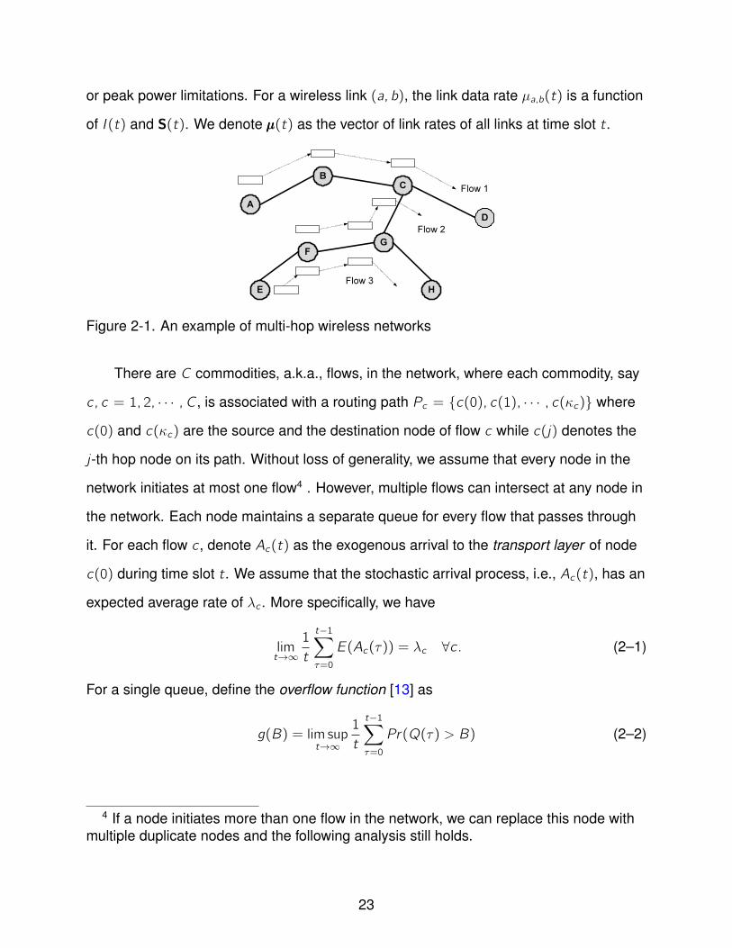
Figure 2-1. An example of multi-hop wireless networks
There are C commodities, a.k.a., flows, in the network, where each commodity, say
c , c = 1, 2, · · · ,C , is associated with a routing path Pc = c(0), c(1), · · · , c(κc) where
c(0) and c(κc) are the source and the destination node of flow c while c(j) denotes the
j-th hop node on its path. Without loss of generality, we assume that every node in the
network initiates at most one flow4 . However, multiple flows can intersect at any node in
the network. Each node maintains a separate queue for every flow that passes through
it. For each flow c , denote Ac(t) as the exogenous arrival to the transport layer of node
c(0) during time slot t. We assume that the stochastic arrival process, i.e., Ac(t), has an
expected average rate of λc . More specifically, we have
limt→∞
1
t
t−1∑τ=0
E(Ac(τ)) = λc ∀c. (2–1)
For a single queue, define the overflow function [13] as
g(B) = lim supt→∞
1
t
t−1∑τ=0
Pr(Q(τ) > B) (2–2)
4 If a node initiates more than one flow in the network, we can replace this node withmultiple duplicate nodes and the following analysis still holds.
23
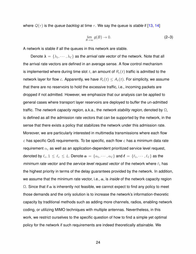
where Q(τ) is the queue backlog at time τ . We say the queue is stable if [13, 14]
limB→∞
g(B)→ 0. (2–3)
A network is stable if all the queues in this network are stable.
Denote λλλ = λ1, · · · ,λC as the arrival rate vector of the network. Note that all
the arrival rate vectors are defined in an average sense. A flow control mechanism
is implemented where during time slot t, an amount of Rc(t) traffic is admitted to the
network layer for flow c . Apparently, we have Rc(t) ≤ Ac(t). For simplicity, we assume
that there are no reservoirs to hold the excessive traffic, i.e., incoming packets are
dropped if not admitted. However, we emphasize that our analysis can be applied to
general cases where transport layer reservoirs are deployed to buffer the un-admitted
traffic. The network capacity region, a.k.a., the network stability region, denoted by Ω,
is defined as all the admission rate vectors that can be supported by the network, in the
sense that there exists a policy that stabilizes the network under this admission rate.
Moreover, we are particularly interested in multimedia transmissions where each flow
c has specific QoS requirements. To be specific, each flow c has a minimum data rate
requirement αc as well as an application-dependent prioritized service level request,
denoted by ℓc , 1 ≤ ℓc ≤ L. Denote ααα = α1, · · · ,αC and ℓℓℓ = ℓ1, · · · , ℓC as the
minimum rate vector and the service level request vector of the network where ℓ1 has
the highest priority in terms of the delay guarantees provided by the network. In addition,
we assume that the minimum rate vector, i.e., ααα, is inside of the network capacity region
Ω. Since that if ααα is inherently not feasible, we cannot expect to find any policy to meet
those demands and the only solution is to increase the network’s information-theoretic
capacity by traditional methods such as adding more channels, radios, enabling network
coding, or utilizing MIMO techniques with multiple antennas. Nevertheless, in this
work, we restrict ourselves to the specific question of how to find a simple yet optimal
policy for the network if such requirements are indeed theoretically attainable. We
24
emphasize that, however, the answer to this question is by no means straightforward
due to the intractability of quantifying the underlying network capacity region. Moreover,
time varying channel conditions and stochastic exogenous arrivals make the problem
even more challenging. It is our main objective to develop an optimum policy without
knowing the network capacity region and the statistical characteristics of random arrival
processes as well as time varying channels. We will formulate the QoS-aware revenue
maximization problem next.
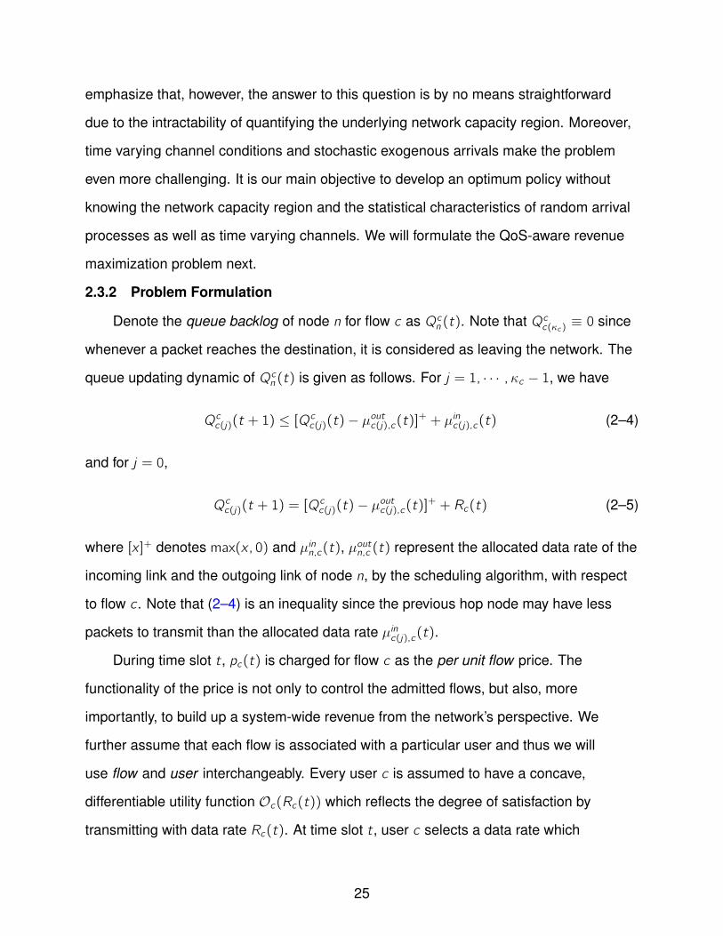
2.3.2 Problem Formulation
Denote the queue backlog of node n for flow c as Qcn (t). Note that Qcc(κc) ≡ 0 since
whenever a packet reaches the destination, it is considered as leaving the network. The
queue updating dynamic of Qcn (t) is given as follows. For j = 1, · · · ,κc − 1, we have
Qcc(j)(t + 1) ≤ [Qcc(j)(t)− µoutc(j),c(t)]+ + µinc(j),c(t) (2–4)
and for j = 0,
Qcc(j)(t + 1) = [Qcc(j)(t)− µoutc(j),c(t)]
+ + Rc(t) (2–5)
where [x ]+ denotes max(x , 0) and µinn,c(t), µoutn,c (t) represent the allocated data rate of the
incoming link and the outgoing link of node n, by the scheduling algorithm, with respect
to flow c . Note that (2–4) is an inequality since the previous hop node may have less
packets to transmit than the allocated data rate µinc(j),c(t).
During time slot t, pc(t) is charged for flow c as the per unit flow price. The
functionality of the price is not only to control the admitted flows, but also, more
importantly, to build up a system-wide revenue from the network’s perspective. We
further assume that each flow is associated with a particular user and thus we will
use flow and user interchangeably. Every user c is assumed to have a concave,
differentiable utility function Oc(Rc(t)) which reflects the degree of satisfaction by
transmitting with data rate Rc(t). At time slot t, user c selects a data rate which
25

optimizes the net income, a.k.a., surplus, i.e.,
Rc(t) = argmaxr (Oc(r)− r × pc(t)) ∀c = 1, · · · ,C . (2–6)
Without loss of generality, we assume that
Oc(r) = log(1 + r). (2–7)
However, we stress that the following analysis can be extended to other heterogeneous
forms of utility functions straightforwardly. Note that the fairness issue of multiple flows
can be solved by choosing utility functions properly. For example, a utility function
of log(r) represents the proportional fairness among competitive flows. For more
discussions, refer to [4] and [10].
From the network administrator’s perspective, the overall network-wide revenue
is the target to be maximized. Meanwhile, the stability of the network as well as the
QoS requirements from multimedia flows need to be addressed. Formally speaking, the
objective of the network is to find an optimal policy to
QoS-Aware Revenue Maximization Problem:
maximize D = lim inft→∞
1
t
t−1∑τ=0
O(τ) (2–8)
s.t.
(a) the network is stable,
(b) the minimum data rate requirements, i.e., ααα, are satisfied,
(c) the guaranteed maximum end-to-end delays for multiple multimedia flows areprioritized according to the service levels of ℓℓℓ,
where
O(t) = E(∑c
Rc(t)pc(t)) (2–9)
is the expected overall network revenue during time slot t, with respected to the
randomness of arrival processes and channel variations.
26
1λ
2λ
Original Feasible Region
Reduced Feasible Region*λ
*λ1α
2α
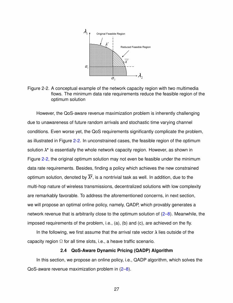
Figure 2-2. A conceptual example of the network capacity region with two multimediaflows. The minimum data rate requirements reduce the feasible region of theoptimum solution
However, the QoS-aware revenue maximization problem is inherently challenging
due to unawareness of future random arrivals and stochastic time varying channel
conditions. Even worse yet, the QoS requirements significantly complicate the problem,
as illustrated in Figure 2-2. In unconstrained cases, the feasible region of the optimum
solution λ∗λ∗λ∗ is essentially the whole network capacity region. However, as shown in
Figure 2-2, the original optimum solution may not even be feasible under the minimum
data rate requirements. Besides, finding a policy which achieves the new constrained
optimum solution, denoted by λ∗λ∗λ∗, is a nontrivial task as well. In addition, due to the
multi-hop nature of wireless transmissions, decentralized solutions with low complexity
are remarkably favorable. To address the aforementioned concerns, in next section,
we will propose an optimal online policy, namely, QADP, which provably generates a
network revenue that is arbitrarily close to the optimum solution of (2–8). Meanwhile, the
imposed requirements of the problem, i.e., (a), (b) and (c), are achieved on the fly.
In the following, we first assume that the arrival rate vector λλλ lies outside of the
capacity region Ω for all time slots, i.e., a heave traffic scenario.
2.4 QoS-Aware Dynamic Pricing (QADP) Algorithm
In this section, we propose an online policy, i.e., QADP algorithm, which solves the
QoS-aware revenue maximization problem in (2–8).
27
We first introduce some system-wide parameters to facilitate our analysis. Define
Rmaxc as the upper bound of admitted traffic of flow c during one time slot, i.e., Rc(t) ≤
Rmaxc ,∀c , t. For example, Rmaxc can represent the hardware limitation on the maximum
volume of traffic that a node can admit during one time slot, or simply the peak arrival
rate within one time slot if such information is available. Let µmax be the maximum data
rate on any link of the network, which may be determined by factors such as the number
of antennas, modulation schemes and coding policies. In addition, for each flow c , we
introduce a virtual queue Yc(t) which is initially empty, and the queue updating dynamic
is defined as
Yc(t + 1) = [Yc(t)− Rc(t)]+ + αc ∀c . (2–10)
Note that virtual queues are easy to implement. For example, the source node of flow
c , i.e., c(0), can maintain a software based counter to measure the backlog updates of
virtual queue Yc(t). In addition, for each flow c , we define
δc = N(µmax)2 + (Rmaxc )
2 +1
2(αc)
2 ∀c . (2–11)
Denote θ1, · · · , θC as the weights which will be calculated and assigned to all flows,
where C denotes the number of flows in the network. Let J be a tunable5 positive large
number determined by the network. In addition, we assume a maximum value of the
allocated weight, denoted by θmax, i.e., θc ≤ θmax,∀c . The proposed QADP algorithm is
given as follows.
QADP ALGORITHM:
- Part I: Weight AssignmentFor all multimedia transmissions, find the flow with the minimum value of αc ×ℓc , c = 1, · · · ,C , say, flow j . For each flow c , assign an associated weight, denoted
5 The impact of J on the performance of QADP algorithm will be clarified shortly.
28
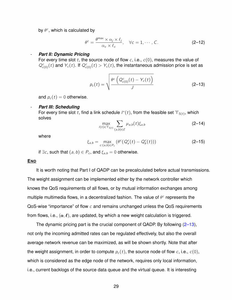
by θc , which is calculated by
θc =θmax × αj × ℓj
αc × ℓc, ∀c = 1, · · · ,C . (2–12)
- Part II: Dynamic PricingFor every time slot t, the source node of flow c , i.e., c(0), measures the value ofQcc(0)(t) and Yc(t). If Qcc(0)(t) > Yc(t), the instantaneous admission price is set as
pc(t) =
√√√√θc(Qcc(0)(t)− Yc(t)
)J
(2–13)
and pc(t) = 0 otherwise.
- Part III: SchedulingFor every time slot t, find a link schedule I ∗(t), from the feasible set ΥS(t), whichsolves
maxI (t)∈ΥS(t)
∑(a,b)∈E
µa,b(t)ξa,b (2–14)
whereξa,b = max
c:(a,b)∈Pc(θc(Qca (t)−Qcb (t))) (2–15)
if ∃c , such that (a, b) ∈ Pc , and ξa,b = 0 otherwise.
END
It is worth noting that Part I of QADP can be precalculated before actual transmissions.
The weight assignment can be implemented either by the network controller which
knows the QoS requirements of all flows, or by mutual information exchanges among
multiple multimedia flows, in a decentralized fashion. The value of θc represents the
QoS-wise “importance” of flow c and remains unchanged unless the QoS requirements
from flows, i.e., (ααα,ℓℓℓ), are updated, by which a new weight calculation is triggered.
The dynamic pricing part is the crucial component of QADP. By following (2–13),
not only the incoming admitted rates can be regulated effectively, but also the overall
average network revenue can be maximized, as will be shown shortly. Note that after
the weight assignment, in order to compute pc(t), the source node of flow c , i.e., c(0),
which is considered as the edge node of the network, requires only local information,
i.e., current backlogs of the source data queue and the virtual queue. It is interesting
29
to observe that if Qcc(0)(t) ≤ Yc(t), the admission is free! Intuitively, a small value of
Qcc(0)(t) indicates a deficient arrival rate of flow c . On the contrary, a large value of Yc(t)
means that the average “service rate” is less than the average “arrival rate” and thus
the virtual queue is building up. Note in (2–10) that this indicates that the average of
Rc(t) falls below the arrival rate, i.e., αc . Therefore, when Qcc(0)(t) ≤ Yc(t), the network
provides free admission to encourage more incoming packets in order to satisfy the QoS
constraints. We will make this intuition precise and rigorous in the following section.
The third part of QADP is a weighted extension to the well-known MaxWeight
scheduling algorithm [12, 13, 34]. Instead of the exact difference of queue backlogs,
we deliberately select the weighted difference of queue backlogs as the weight of a
particular link in the scheduling algorithm. Intuitively, if a flow is assigned with a larger
value of θc , the links associated with it will have a higher possibility of being selected
for transmissions by QADP. Therefore, by assigning proper values of θc to flows with
different QoS requirements, a service differentiation can be achieved which provides
more flexibility to previous schemes in the literature, e.g., [13, 15, 16]. In addition,
as indicated by (2–13), a higher priority needs to pay at a higher price. Note that to
calculate (2–14), QADP needs to solve a complex optimization problem which requires
a global information on channel states, i.e., S(t). However, availed of the prosperous
development of distributed scheduling schemes, such as [35–38], the difficulty of
centralized computation can be circumvented, which provides QADP algorithm the
amenability for decentralized implementations.
2.5 Performance Analysis
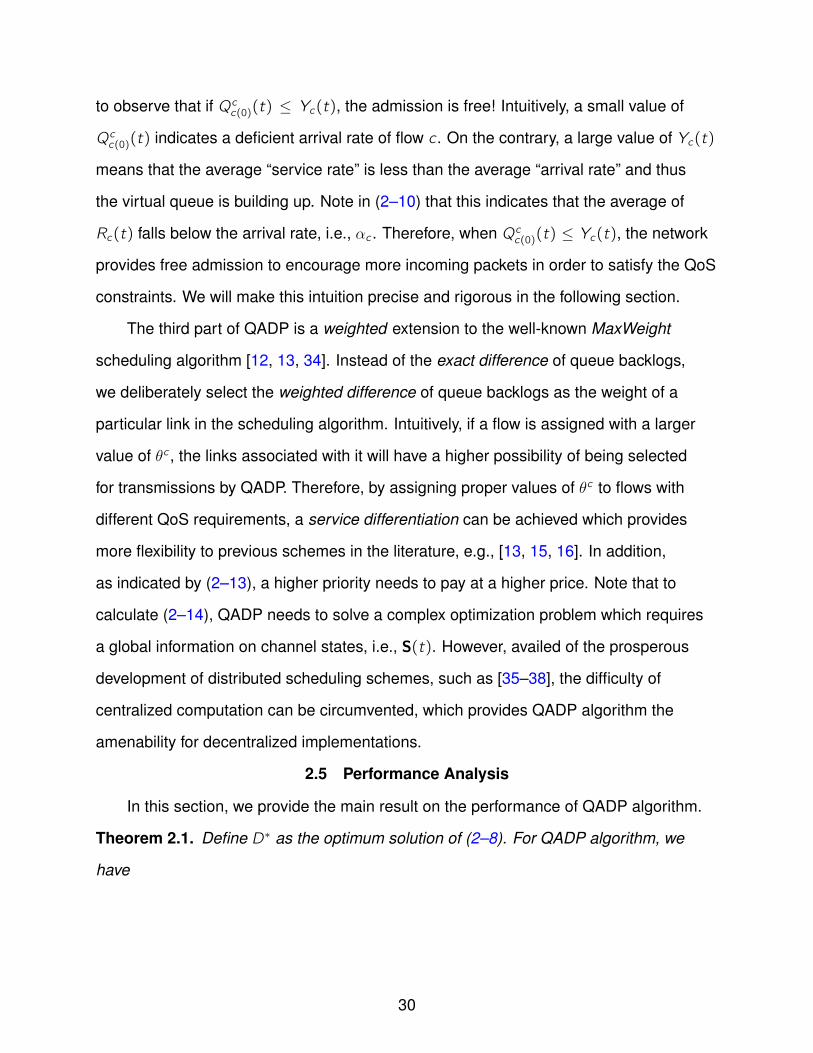
In this section, we provide the main result on the performance of QADP algorithm.
Theorem 2.1. Define D∗ as the optimum solution of (2–8). For QADP algorithm, we
have
30
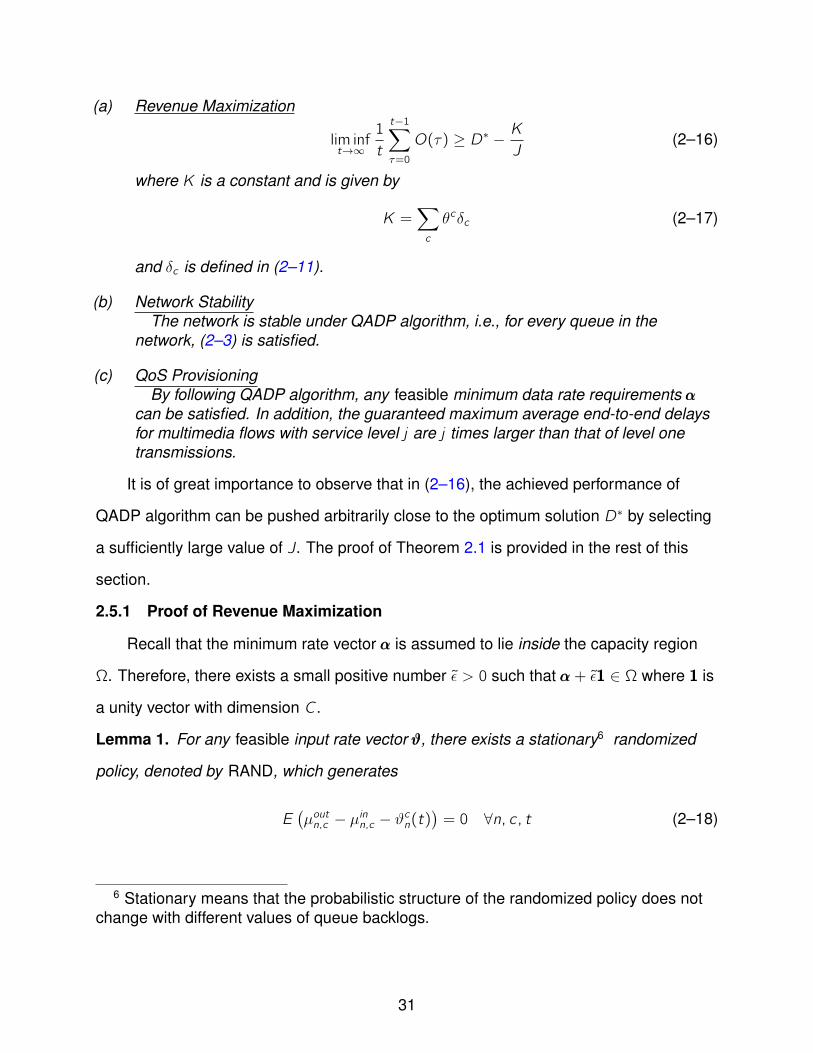
(a) Revenue Maximization
lim inft→∞
1
t
t−1∑τ=0
O(τ) ≥ D∗ − KJ
(2–16)
where K is a constant and is given by
K =∑c
θcδc (2–17)
and δc is defined in (2–11).
(b) Network StabilityThe network is stable under QADP algorithm, i.e., for every queue in the
network, (2–3) is satisfied.
(c) QoS ProvisioningBy following QADP algorithm, any feasible minimum data rate requirements ααα
can be satisfied. In addition, the guaranteed maximum average end-to-end delaysfor multimedia flows with service level j are j times larger than that of level onetransmissions.
It is of great importance to observe that in (2–16), the achieved performance of
QADP algorithm can be pushed arbitrarily close to the optimum solution D∗ by selecting
a sufficiently large value of J. The proof of Theorem 2.1 is provided in the rest of this
section.
2.5.1 Proof of Revenue Maximization
Recall that the minimum rate vector ααα is assumed to lie inside the capacity region
Ω. Therefore, there exists a small positive number ϵ > 0 such that ααα + ϵ1 ∈ Ω where 1 is
a unity vector with dimension C .
Lemma 1. For any feasible input rate vector ϑϑϑ, there exists a stationary6 randomized
policy, denoted by RAND, which generates
E(µoutn,c − µinn,c − ϑcn(t)
)= 0 ∀n, c , t (2–18)
6 Stationary means that the probabilistic structure of the randomized policy does notchange with different values of queue backlogs.
31
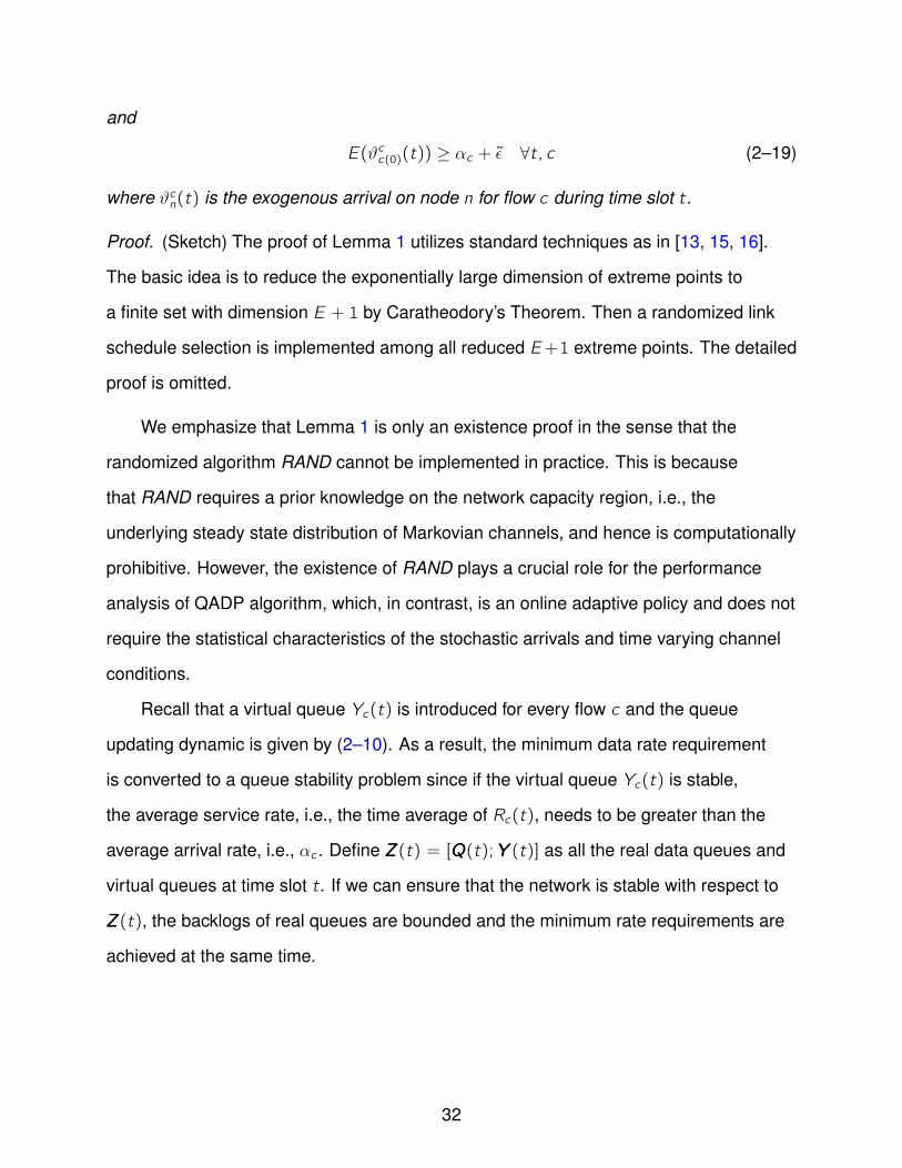
and
E(ϑcc(0)(t)) ≥ αc + ϵ ∀t, c (2–19)
where ϑcn(t) is the exogenous arrival on node n for flow c during time slot t.
Proof. (Sketch) The proof of Lemma 1 utilizes standard techniques as in [13, 15, 16].
The basic idea is to reduce the exponentially large dimension of extreme points to
a finite set with dimension E + 1 by Caratheodory’s Theorem. Then a randomized link
schedule selection is implemented among all reduced E+1 extreme points. The detailed
proof is omitted.
We emphasize that Lemma 1 is only an existence proof in the sense that the
randomized algorithm RAND cannot be implemented in practice. This is because
that RAND requires a prior knowledge on the network capacity region, i.e., the
underlying steady state distribution of Markovian channels, and hence is computationally
prohibitive. However, the existence of RAND plays a crucial role for the performance
analysis of QADP algorithm, which, in contrast, is an online adaptive policy and does not
require the statistical characteristics of the stochastic arrivals and time varying channel
conditions.
Recall that a virtual queue Yc(t) is introduced for every flow c and the queue
updating dynamic is given by (2–10). As a result, the minimum data rate requirement
is converted to a queue stability problem since if the virtual queue Yc(t) is stable,
the average service rate, i.e., the time average of Rc(t), needs to be greater than the
average arrival rate, i.e., αc . Define ZZZ(t) = [QQQ(t);YYY (t)] as all the real data queues and
virtual queues at time slot t. If we can ensure that the network is stable with respect to
ZZZ(t), the backlogs of real queues are bounded and the minimum rate requirements are
achieved at the same time.
32
Define a system-wide potential function (PF) as
PF (ZZZ(t)) =∑c
PF c(ZZZ(t)) (2–20)
where
PF c(ZZZ(t)) =1
2
(∑n
θc(Qcn (t))2 + θc(Yc(t))
2
). (2–21)
Note that PF (ZZZ(t)) is a scalar-valued nonnegative function. Define
∆(ZZZ(t)) = E (PF (ZZZ(t + 1))− PF (ZZZ(t))|ZZZ(t)) (2–22)
as the drift of the potential function PF (ZZZ(t)).
For flow c , we take the square of both sides of (2–4) and (2–5) and obtain7
(Qcc(j)(t + 1)
)2 ≤ (Qcc(j)(t))2 + (µoutc(j),c(t))2+(µinc(j),c(t)
)2 − 2Qcc(j)(t) (µoutc(j),c(t)− µinc(j),c(t))
for j = 1, · · · ,κc − 1, and
(Qcc(j)(t + 1)
)2 ≤ (Qcc(j)(t))2 + (µoutc(j),c(t))2+(Rc(t))
2 − 2Qcc(j)(t)(µoutc(j),c(t)− Rc(t)
)(2–23)
for j = 0. Similarly, for (2–10), we have
(Yc(t + 1))2 ≤ (Yc(t))
2 + (Rc(t))2 + (αc)
2
−2Yc(t)(Rc(t)− αc). (2–24)
7 We use the fact that for nonnegative real numbers a, b, c , d , if a ≤ [b − c ]+ + d , thena2 ≤ b2 + c2 + d2 − 2b(c − d), as given in Lemma 4.3 on [17].
33
By combining the inequalities above, we have
PF c(ZZZ(t + 1))− PF c(ZZZ(t))
≤ Ξc + θcQcc(0)(t)Rc(t)− θcYc(t)(Rc(t)− αc)
−∑n
θcQcn (t)(µoutn,c (t)− µinn,c(t)
)(2–25)
where
Ξc = θc(N(µmax)2 + (Rmaxc )
2 +1
2(αc)
2
). (2–26)
Note that (2–25) is summed over the whole network. If node n is not on the path of
flow c , µinn,c(t) = µoutn,c (t) = 0. Moreover, µinn,c(t) = 0 for the source node of flow c and
µoutn,c (t) = 0 for the destination node of flow c . Next, we sum over all flows to derive the
network-wide potential function difference as
PF (ZZZ(t + 1))− PF (ZZZ(t))
≤ K −∑n,c
θcQcn (t)(µoutn,c (t)− µinn,c(t))
+∑c
θcQcc(0)(t)Rc(t)−∑c
θcYc(t)(Rc(t)− αc)
where K =∑c Ξc . Therefore, we have
∆(ZZZ(t)) ≤ K −∑n,c
θcQcn (t)E(µoutn,c (t)− µinn,c(t)|ZZZ(t)
)+
∑c
θcQcc(0)(t)E(Rc(t)|ZZZ(t))
−∑c
θcYc(t)E(Rc(t)− αc |ZZZ(t)). (2–27)
34
Next, for a positive constant J, we subtract both sides of (2–27) by JE(∑
c Rc(t)pc(t)|ZZZ(t))
and have
∆(ZZZ(t))− JE
(∑c
Rc(t)pc(t)|ZZZ(t)
)≤ K −
∑n,c
θcQcn (t)E(µoutn,c (t)− µinn,c(t)|ZZZ(t)
)+∑c
θcQcc(0)(t)E(Rc(t)|ZZZ(t))
−∑c
θcYc(t)E(Rc(t)− αc |ZZZ(t))
−JE
(∑c
Rc(t)pc(t)|ZZZ(t)
). (2–28)
Note that (2–28) is general and holds for any possible policy.
For an arbitrarily small positive constant 0 < ϵ ≤ ϵmax, define the ϵ-reduced network
capacity region, Ωϵ, as all possible input rate vectors such that
Ωϵ = λλλ|λc + ϵ ∈ Ω ∀c (2–29)
where Ω is the original network capacity region. We will discuss about how to obtain ϵmax
shortly.
Define D∗ϵ as the optimum value of the reduced problem to (2–8) where Ω is
replaced by Ωϵ. It can be verified that [14]
limϵ→0D∗
ϵ → D∗ (2–30)
where D∗ is the optimum value of the original revenue maximization problem in (2–8),
i.e., the target of QADP algorithm.
Specifically, we denote r ∗ϵ,c(0), r ∗ϵ,c(1), · · · , r ∗ϵ,c(t), · · · and p∗ϵ,c(0), p∗ϵ,c(1), · · · , p∗ϵ,c(t), · · ·
as the optimum sequences of admitted rates and prices, for flow c , which achieve D∗ϵ .
Define r ϵc as the time average of the optimum sequence of r ∗ϵ,c(0), r ∗ϵ,c(1), · · · , r ∗ϵ,c(t), · · · .
Therefore, following the definition of (2–29), we have r ϵc + ϵ ∈ Ω. By Lemma 1, we claim
35
that there exists a randomized policy, denoted by RAND, which yields
E(µoutn,c (t)− µinn,c(t)− r ∗ϵ,c(t)) = ϵ ∀c , n = c(0) (2–31)
and
E(µoutn,c (t)− µinn,c(t)) = ϵ ∀c , n = c(0) (2–32)
and
E(r ∗ϵ,c(t) + ϵ) ≥ αc + ϵ ∀c . (2–33)
Denote the RHS of (2–28) as Ψ. Without loss of generality, we assume ϵ ≤ ϵ. Therefore,
for randomized policy RAND, we have
ΨRAND ≤ K − ϵ
(∑n,c
θcQcn (t) +∑c
θcYc(t)
)
−JE
(∑c
(r ∗ϵ,c(t) + ϵ)p∗ϵ,c(t)|ZZZ(t)
)(2–34)
where p∗ϵ,c(t) is the corresponding price which induces a rate of r ∗ϵ,c(t) + ϵ by (2–6).
Lemma 2. QADP algorithm minimizes the RHS of (2–28) over all possible policies.
Proof. The scheduling part of QADP algorithm in Section 2.4 is a weighted version of
MaxWeight algorithm [12, 13, 34] which maximizes∑n,c θ
cQcn (t)(µoutn,c (t) − µinn,c(t)) =∑
(a,b)∈E µa,b(t)ξa,b if ∃c , such that (a, b) ∈ Pc , for every time slot t. The dynamic pricing
part of QADP is essentially maximizing
∑c
(θc(Yc(t)−Qcc(0)(t))Rc(t) + JRc(t)pc(t)
)(2–35)
for every time slot. By (2–6) and (2–7), we see that QADP finds an optimum price p∗c(t)
which maximizes
M = θc(Yc(t)−Qcc(0)(t))(1
pc(t)− 1) + J(1− pc(t)). (2–36)
DefineW = θc(Qcc(0)(t)− Yc(t)).
36
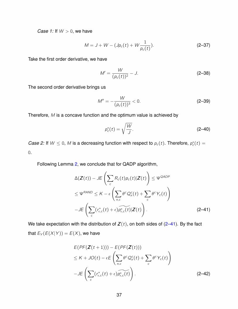
Case 1: IfW > 0, we have
M = J +W − (Jpc(t) +W1
pc(t)). (2–37)
Take the first order derivative, we have
M ′ =W
(pc(t))2− J. (2–38)
The second order derivative brings us
M ′′ = − W
(pc(t))3< 0. (2–39)
Therefore, M is a concave function and the optimum value is achieved by
p∗c(t) =
√W
J. (2–40)
Case 2: IfW ≤ 0, M is a decreasing function with respect to pc(t). Therefore, p∗c(t) =
0.
Following Lemma 2, we conclude that for QADP algorithm,
∆(ZZZ(t))− JE
(∑c
Rc(t)pc(t)|ZZZ(t)
)≤ ΨQADP
≤ ΨRAND ≤ K − ϵ
(∑n,c
θcQcn (t) +∑c
θcYc(t)
)
−JE
(∑c
(r ∗ϵ,c(t) + ϵ)p∗ϵ,c(t)|ZZZ(t)
). (2–41)
We take expectation with the distribution of ZZZ(t), on both sides of (2–41). By the fact
that EY (E(X |Y )) = E(X ), we have
E(PF (ZZZ(t + 1)))− E(PF (ZZZ(t)))
≤ K + JO(t)− ϵE
(∑n,c
θcQcn (t) +∑c
θcYc(t)
)
−JE
(∑c
(r ∗ϵ,c(t) + ϵ)p∗ϵ,c(t)
). (2–42)
37
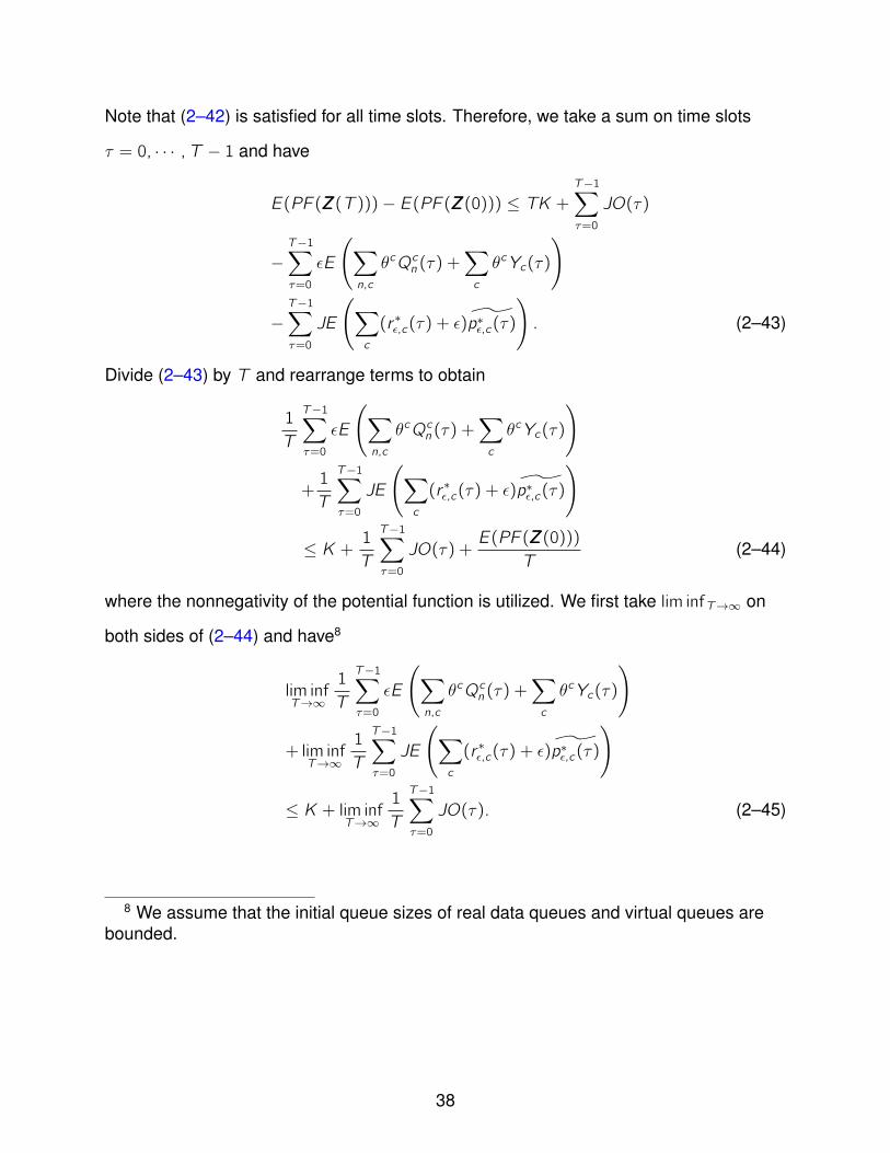
Note that (2–42) is satisfied for all time slots. Therefore, we take a sum on time slots
τ = 0, · · · ,T − 1 and have
E(PF (ZZZ(T )))− E(PF (ZZZ(0))) ≤ TK +T−1∑τ=0
JO(τ)
−T−1∑τ=0
ϵE
(∑n,c
θcQcn (τ) +∑c
θcYc(τ)
)
−T−1∑τ=0
JE
(∑c
(r ∗ϵ,c(τ) + ϵ)p∗ϵ,c(τ)
). (2–43)
Divide (2–43) by T and rearrange terms to obtain
1
T
T−1∑τ=0
ϵE
(∑n,c
θcQcn (τ) +∑c
θcYc(τ)
)
+1
T
T−1∑τ=0
JE
(∑c
(r ∗ϵ,c(τ) + ϵ)p∗ϵ,c(τ)
)
≤ K + 1T
T−1∑τ=0
JO(τ) +E(PF (ZZZ(0)))
T(2–44)
where the nonnegativity of the potential function is utilized. We first take lim infT→∞ on
both sides of (2–44) and have8
lim infT→∞
1
T
T−1∑τ=0
ϵE
(∑n,c
θcQcn (τ) +∑c
θcYc(τ)
)
+ lim infT→∞
1
T
T−1∑τ=0
JE
(∑c
(r ∗ϵ,c(τ) + ϵ)p∗ϵ,c(τ)
)
≤ K + lim infT→∞
1
T
T−1∑τ=0
JO(τ). (2–45)
8 We assume that the initial queue sizes of real data queues and virtual queues arebounded.
38
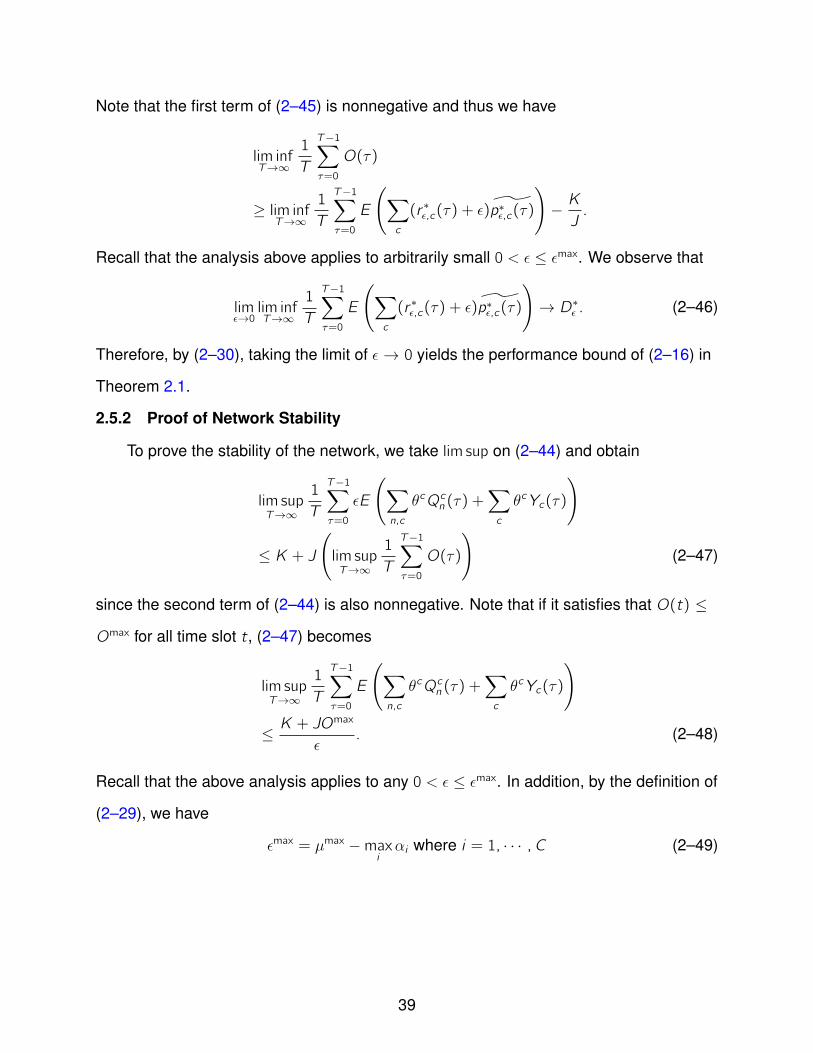
Note that the first term of (2–45) is nonnegative and thus we have
lim infT→∞
1
T
T−1∑τ=0
O(τ)
≥ lim infT→∞
1
T
T−1∑τ=0
E
(∑c
(r ∗ϵ,c(τ) + ϵ)p∗ϵ,c(τ)
)− KJ.
Recall that the analysis above applies to arbitrarily small 0 < ϵ ≤ ϵmax. We observe that
limϵ→0lim infT→∞
1
T
T−1∑τ=0
E
(∑c
(r ∗ϵ,c(τ) + ϵ)p∗ϵ,c(τ)
)→ D∗
ϵ . (2–46)
Therefore, by (2–30), taking the limit of ϵ → 0 yields the performance bound of (2–16) in
Theorem 2.1.
2.5.2 Proof of Network Stability
To prove the stability of the network, we take lim sup on (2–44) and obtain
lim supT→∞
1
T
T−1∑τ=0
ϵE
(∑n,c
θcQcn (τ) +∑c
θcYc(τ)
)
≤ K + J
(lim supT→∞
1
T
T−1∑τ=0
O(τ)
)(2–47)
since the second term of (2–44) is also nonnegative. Note that if it satisfies that O(t) ≤
Omax for all time slot t, (2–47) becomes
lim supT→∞
1
T
T−1∑τ=0
E
(∑n,c
θcQcn (τ) +∑c
θcYc(τ)
)
≤ K + JOmax
ϵ. (2–48)
Recall that the above analysis applies to any 0 < ϵ ≤ ϵmax. In addition, by the definition of
(2–29), we have
ϵmax = µmax −maxiαi where i = 1, · · · ,C (2–49)
39
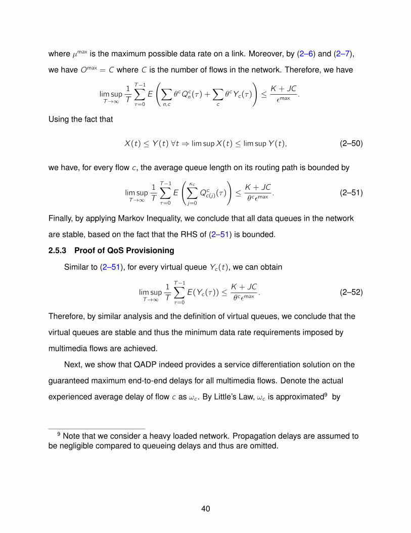
where µmax is the maximum possible data rate on a link. Moreover, by (2–6) and (2–7),
we have Omax = C where C is the number of flows in the network. Therefore, we have
lim supT→∞
1
T
T−1∑τ=0
E
(∑n,c
θcQcn (τ) +∑c
θcYc(τ)
)≤ K + JC
ϵmax.
Using the fact that
X (t) ≤ Y (t) ∀t ⇒ lim supX (t) ≤ lim supY (t), (2–50)
we have, for every flow c , the average queue length on its routing path is bounded by
lim supT→∞
1
T
T−1∑τ=0
E
(κc∑j=0
Qcc(j)(τ)
)≤ K + JC
θcϵmax. (2–51)
Finally, by applying Markov Inequality, we conclude that all data queues in the network
are stable, based on the fact that the RHS of (2–51) is bounded.
2.5.3 Proof of QoS Provisioning
Similar to (2–51), for every virtual queue Yc(t), we can obtain
lim supT→∞
1
T
T−1∑τ=0
E(Yc(τ)) ≤K + JC
θcϵmax. (2–52)
Therefore, by similar analysis and the definition of virtual queues, we conclude that the
virtual queues are stable and thus the minimum data rate requirements imposed by
multimedia flows are achieved.
Next, we show that QADP indeed provides a service differentiation solution on the
guaranteed maximum end-to-end delays for all multimedia flows. Denote the actual
experienced average delay of flow c as ωc . By Little’s Law, ωc is approximated9 by
9 Note that we consider a heavy loaded network. Propagation delays are assumed tobe negligible compared to queueing delays and thus are omitted.
40
ωc =average overall queue length on the path of flow c
average incoming rate of flow c
=lim supT→∞
1T
∑T−1τ=0 E
(∑κcj=0Q
cc(j)(τ)
)lim supT→∞
1T
∑T−1τ=0 E(Rc(τ))
. (2–53)
In light of the stability of virtual queue Yc(t), we have lim supT→∞1T
∑T−1τ=0 E(Rc(τ)) ≥
αc . Hence, we can obtain
ωc ≤K + JC
θcϵmaxαc. (2–54)
Equivalently speaking, to differentiate the guaranteed maximum delay bound, we need
to find a set of weights such that
θcαcℓc = θdαdℓd (2–55)
is satisfied for any pair of multimedia flows c and d . Therefore, it is straightforward
to verify that the weight assignment algorithm in QADP indeed provides a service
differentiation solution where the guaranteed maximum end-to-end delays of multimedia
flows are distinguished according to application-dependent service level requests,
which completes the proof of Theorem 2.1. The performance of QADP algorithm will be
evaluated numerically in Section 2.6.
2.6 Simulations
2.6.1 Single-Hop Wireless Cellular Networks
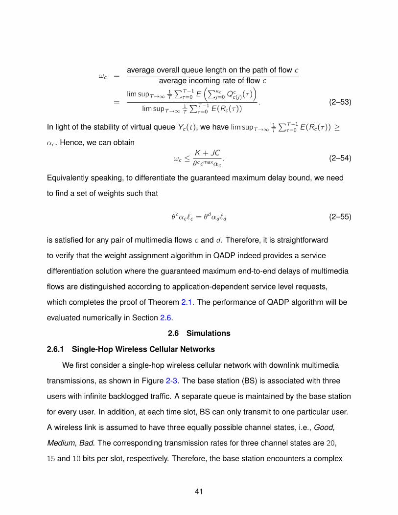
We first consider a single-hop wireless cellular network with downlink multimedia
transmissions, as shown in Figure 2-3. The base station (BS) is associated with three
users with infinite backlogged traffic. A separate queue is maintained by the base station
for every user. In addition, at each time slot, BS can only transmit to one particular user.
A wireless link is assumed to have three equally possible channel states, i.e., Good,
Medium, Bad. The corresponding transmission rates for three channel states are 20,
15 and 10 bits per slot, respectively. Therefore, the base station encounters a complex
41
opportunistic scheduling problem where the revenue maximization problem, network
stability as well as the QoS requirements need to be addressed simultaneously.
Good, Medium, Bad
Base Station1 2 3
User 1 User 2 User 3
Figure 2-3. A single-hop wireless cellular network with three users
Without loss of generality, we assume that the minimum average rate requirements
for user 1, 2, 3 are ααα = [1, 2, 3] bits per slot. In addition, to provide service differentiation,
the network offers three prioritized service levels, e.g., Platinum, Gold and Silver,
where level Platinum possesses the highest priority in terms of end-to-end delay upper
bound. We assume that user 1 has a service level request for Platinum while user
2 and 3 demand for level Gold and Silver, respectively, according to the upper layer
applications. Other system parameters are assumed to be Rmaxc = 20 bits per slot for
all flows and θmax = 100. We next implement QADP algorithm for different values of J
where J = [50, 100, 500, 1000, 5000, 10000, 20000, 50000, 100000]. Every experiment is
simulated for 500000 time slots.
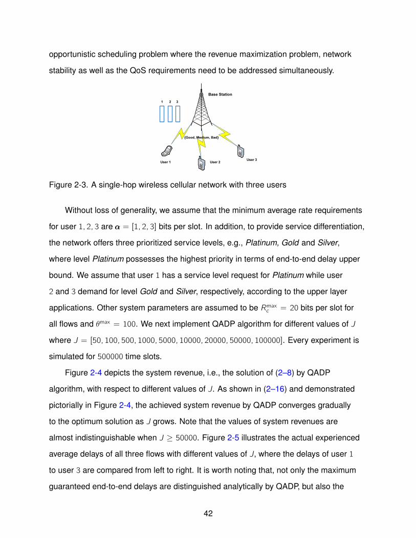
Figure 2-4 depicts the system revenue, i.e., the solution of (2–8) by QADP
algorithm, with respect to different values of J. As shown in (2–16) and demonstrated
pictorially in Figure 2-4, the achieved system revenue by QADP converges gradually
to the optimum solution as J grows. Note that the values of system revenues are
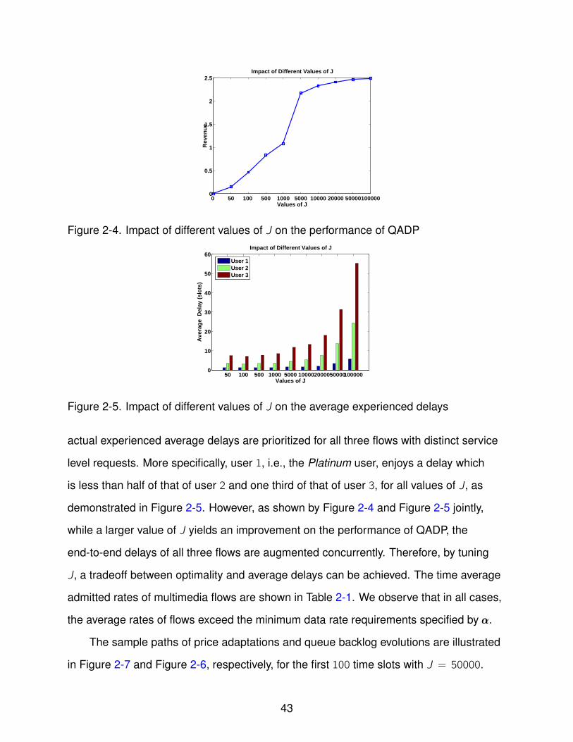
almost indistinguishable when J ≥ 50000. Figure 2-5 illustrates the actual experienced
average delays of all three flows with different values of J, where the delays of user 1
to user 3 are compared from left to right. It is worth noting that, not only the maximum
guaranteed end-to-end delays are distinguished analytically by QADP, but also the
42
0 50 100 500 1000 5000 10000 20000 500001000000
0.5
1
1.5
2
2.5
Values of JR
even
ue
Impact of Different Values of J
Figure 2-4. Impact of different values of J on the performance of QADP
50 100 500 1000 5000 1000020000500001000000
10
20
30
40
50
60
Values of J
Ave
rag
e D
elay
(sl
ots
)
Impact of Different Values of J
User 1User 2User 3
Figure 2-5. Impact of different values of J on the average experienced delays
actual experienced average delays are prioritized for all three flows with distinct service
level requests. More specifically, user 1, i.e., the Platinum user, enjoys a delay which
is less than half of that of user 2 and one third of that of user 3, for all values of J, as
demonstrated in Figure 2-5. However, as shown by Figure 2-4 and Figure 2-5 jointly,
while a larger value of J yields an improvement on the performance of QADP, the
end-to-end delays of all three flows are augmented concurrently. Therefore, by tuning
J, a tradeoff between optimality and average delays can be achieved. The time average
admitted rates of multimedia flows are shown in Table 2-1. We observe that in all cases,
the average rates of flows exceed the minimum data rate requirements specified by ααα.
The sample paths of price adaptations and queue backlog evolutions are illustrated
in Figure 2-7 and Figure 2-6, respectively, for the first 100 time slots with J = 50000.
43
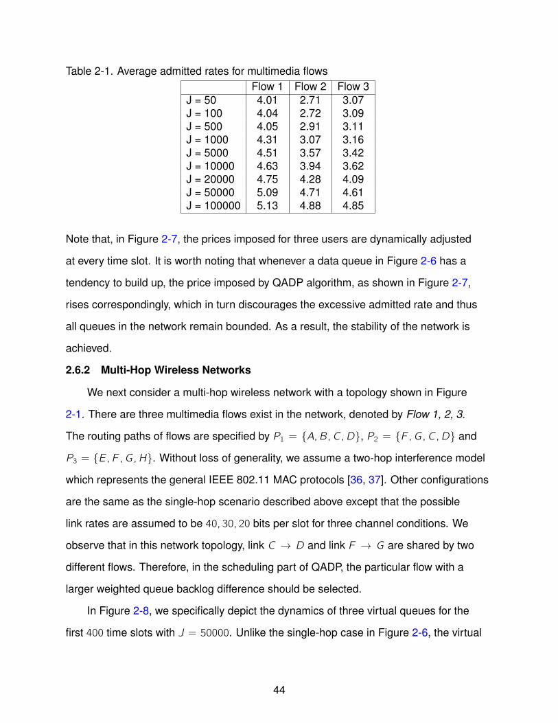
Table 2-1. Average admitted rates for multimedia flowsFlow 1 Flow 2 Flow 3
J = 50 4.01 2.71 3.07J = 100 4.04 2.72 3.09J = 500 4.05 2.91 3.11J = 1000 4.31 3.07 3.16J = 5000 4.51 3.57 3.42J = 10000 4.63 3.94 3.62J = 20000 4.75 4.28 4.09J = 50000 5.09 4.71 4.61J = 100000 5.13 4.88 4.85
Note that, in Figure 2-7, the prices imposed for three users are dynamically adjusted
at every time slot. It is worth noting that whenever a data queue in Figure 2-6 has a
tendency to build up, the price imposed by QADP algorithm, as shown in Figure 2-7,
rises correspondingly, which in turn discourages the excessive admitted rate and thus
all queues in the network remain bounded. As a result, the stability of the network is
achieved.
2.6.2 Multi-Hop Wireless Networks
We next consider a multi-hop wireless network with a topology shown in Figure
2-1. There are three multimedia flows exist in the network, denoted by Flow 1, 2, 3.
The routing paths of flows are specified by P1 = A,B,C ,D, P2 = F ,G ,C ,D and
P3 = E ,F ,G ,H. Without loss of generality, we assume a two-hop interference model
which represents the general IEEE 802.11 MAC protocols [36, 37]. Other configurations
are the same as the single-hop scenario described above except that the possible
link rates are assumed to be 40, 30, 20 bits per slot for three channel conditions. We
observe that in this network topology, link C → D and link F → G are shared by two
different flows. Therefore, in the scheduling part of QADP, the particular flow with a
larger weighted queue backlog difference should be selected.
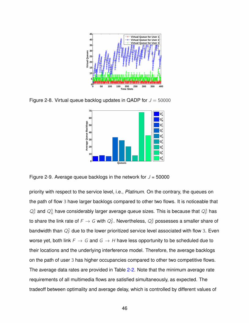
In Figure 2-8, we specifically depict the dynamics of three virtual queues for the
first 400 time slots with J = 50000. Unlike the single-hop case in Figure 2-6, the virtual
44

Figure 2-6. Queue backlog dynamics for all users
0 20 40 60 80 1000
0.1
0.2
0.3
0.4
0.5
0.6
0.7
Time Slots
Pri
ces
Imp
ose
d
price for user 1price for user 2price for user 3
Figure 2-7. Price dynamics in QADP for all users
0 20 40 60 80 1000
10
20
30
40
50
Time Slots
Qu
eue
Bac
klo
gs
Queue 1Virtual Queue 2Queue 2Virtual Queue 3Queue 3Virtual Queue 1
queues behave remarkably different in this multi-hop scenario. It is worth noting that
while the virtual queues of user 1 and 3 have relatively low occupancies, the virtual
queue associated with user 2 suffers a larger average backlog. Intuitively, due to the
underlying two-hop interference model, link G → C needs to be scheduled exclusively
in the network for successful transmissions. In other words, link G → C is the bottleneck
of the network. Therefore, to ensure network-wide stability, a much more stringent
regulation is enforced on the admitted rate of flow 2. As a consequence, although
remains bounded, the virtual queue of flow 2 accumulates more backlogs compared
to other competitive flows. In addition, we compare the time average queue backlogs
of all data queues in the network, from left to right, in Figure 2-9. We can observe that
the data queues on the path of flow 1 have fewer average backlogs due to the highest
45
0 50 100 150 200 250 300 350 4000
5
10
15
20
25
30
35
40
45
Time SlotsV
irtu
al Q
ueu
es
Virtual Queue for User 1Virtual Queue for User 2Virtual Queue for User 3
Figure 2-8. Virtual queue backlog updates in QADP for J = 50000
0
10
20
30
40
50
60
70
Queues
Ave
rag
e Q
ueu
e B
ackl
og
s
QA1
QB1
QC1
QF2
QG2
QC2
QE3
QF3
QG3
Figure 2-9. Average queue backlogs in the network for J = 50000
priority with respect to the service level, i.e., Platinum. On the contrary, the queues on
the path of flow 3 have larger backlogs compared to other two flows. It is noticeable that
Q3F and Q3G have considerably larger average queue sizes. This is because that Q3F has
to share the link rate of F → G with Q2F . Nevertheless, Q3F possesses a smaller share of
bandwidth than Q2F due to the lower prioritized service level associated with flow 3. Even
worse yet, both link F → G and G → H have less opportunity to be scheduled due to
their locations and the underlying interference model. Therefore, the average backlogs
on the path of user 3 has higher occupancies compared to other two competitive flows.
The average data rates are provided in Table 2-2. Note that the minimum average rate
requirements of all multimedia flows are satisfied simultaneously, as expected. The
tradeoff between optimality and average delay, which is controlled by different values of
46

J, as well as the network service differentiation in terms of delays are analogous to the
single-hop scenario discussed above. Duplicated simulation figures are omitted.
Table 2-2. Average admitted rates for multimedia flowsFlow 1 Flow 2 Flow 3
J = 50 3.04 2.08 3.88J = 100 3.12 2.03 3.98J = 500 3.17 2.04 4.60J = 1000 3.30 2.03 5.04J = 5000 4.13 2.01 6.45J = 10000 4.36 2.02 7.32J = 20000 5.08 2.03 8.12J = 50000 6.43 2.01 9.18J = 100000 7.63 2.01 9.89
2.7 Conclusions
We consider a multi-hop wireless network where multiple QoS-specific multimedia
flows share the network resource jointly. To maximize the overall network revenue,
we propose a dynamic pricing based algorithm, namely, QADP, which achieves a
solution that is arbitrarily close to the optimum, subject to network stability. Moreover,
a weight assignment mechanism is introduced to address the service differentiation
issue for multimedia flows with different delay priorities. In tandem with the virtual
queue technique which provides minimum average data rate guarantees, the QoS
requirements of multiple multimedia streams are addressed effectively.
In this work, the application-dependent service level requests and the users’
utility functions are assumed to be attained truthfully. The mechanism design for
strategy-proof user information acquisition seems interesting and needs further
investigation. Moreover, in this work, we assume that the information of channel states,
i.e., S(t), is available for QADP algorithm, which is either acquired by the central base
station or approximated by the distributed local scheduling algorithms. As a future
work, an online channel probing mechanism needs to be incorporated into QADP, as
suggested in [39].
47
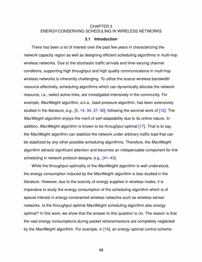
CHAPTER 3ENERGY-CONSERVING SCHEDULING IN WIRELESS NETWORKS
3.1 Introduction
There has been a lot of interest over the past few years in characterizing the
network capacity region as well as designing efficient scheduling algorithms in multi-hop
wireless networks. Due to the stochastic traffic arrivals and time-varying channel
conditions, supporting high throughput and high quality communications in multi-hop
wireless networks is inherently challenging. To utilize the scarce wireless bandwidth
resource effectively, scheduling algorithms which can dynamically allocate the network
resource, i.e., select active links, are investigated intensively in the community. For
example, MaxWeight algorithm, a.k.a., back-pressure algorithm, has been extensively
studied in the literature, e.g., [5, 14, 34, 37, 40], following the seminal work of [12]. The
MaxWeight algorithm enjoys the merit of self-adaptability due to its online nature. In
addition, MaxWeight algorithm is known to be throughput optimal [17]. That is to say,
the MaxWeight algorithm can stabilize the network under arbitrary traffic load that can
be stabilized by any other possible scheduling algorithms. Therefore, the MaxWeight
algorithm attracts significant attention and becomes an indispensable component for link
scheduling in network protocol designs, e.g., [41–43].
While the throughput-optimality of the MaxWeight algorithm is well understood,
the energy consumption induced by the MaxWeight algorithm is less studied in the
literature. However, due to the scarcity of energy supplies in wireless nodes, it is
imperative to study the energy consumption of the scheduling algorithm which is of
special interest in energy-constrained wireless networks such as wireless sensor
networks. Is the throughput optimal MaxWeight scheduling algorithm also energy
optimal? In this work, we show that the answer to this question is no. The reason is that
the vast energy consumptions during packet retransmissions are completely neglected
by the MaxWeight algorithm. For example, in [16], an energy optimal control scheme
48

is proposed where a minimum power expenditure is achieved. However, as in other
related works, e.g., [17], the wireless channels in [16] are assumed to be error-free, i.e.,
all the transmissions are assumed to be successful. Nevertheless, in practice, wireless
channels are error-prone and data transmissions are subject to random failures due to
the hostile channel conditions. Therefore, before a packet can be successfully removed
from the transmitter’s queue, several transmissions may have occurred, including the
original attempt and the posterior retransmissions, which deplete a significant amount
of energy for the transmitter. However, in the traditional MaxWeight algorithm, such
energy-consuming retransmissions induced by channel errors are overlooked. Intuitively,
from energy-saving perspective, the possibility that a particular link is selected for
transmissions should rely on not only the queue difference between the transmitter
and the receiver, which is the design rationale of the traditional MaxWeight algorithm,
but also the potential energy consumptions of retransmissions induced by erroneous
channels. We will make this intuition precise and rigorous in the following sections.
In this work, we propose a minimum energy scheduling (MES) algorithm which
consumes an amount of energy that can be pushed arbitrarily close to the global
minimum solution. In addition, the energy efficiency attained by the MES algorithm
incurs no loss of throughput-optimality. The proposed MES algorithm significantly
reduces the overall energy consumption compared to the traditional MaxWeight
algorithm and remains throughput optimal. Therefore, our proposed MES algorithm is
more favorable for dynamic link scheduling and network protocol designs in energy-constrained
wireless networks such as wireless sensor networks.
The rest of this chapter is organized as follows. Section 3.2 describes the system
model used in this work. The proposed MES algorithm is introduced in Section 3.3
where the performance analysis is provided. Simulation results are shown in Section 3.4
and Section 3.5 concludes this chapter.
49
3.2 System Model
We consider a static multi-hop wireless network denoted by a directed graph (N ,L)
where N is the set of nodes and L denotes the set of links in the network. We use |X |
to represent the cardinality of set X . Time is slotted by t = 0, 1, 2, · · · and in every time
slot, the instantaneous channel state of a link (a, b) ∈ L is denoted by Sa,b(t) where a
and b are the transmitter and the receiver of the link. In this work, we use S(t) to denote
the channel state vector of the whole network. Note that S(t) remains constant within
one time slot, however, it is subject to changes on time slot boundaries. We assume that
S(t) has a finite but potentially large number of possible values and evolves following an
irreducible Markovian chain with well defined steady state distributions. Nevertheless,
the steady state distribution and the transition probabilities are unknown to the network.
Given an instantaneous channel state Sa,b(t), the transmission of a packet on link (a, b)
is successful with a probability of pa,b(t), if link (a, b) is active and suffers no interference
from concurrent transmissions. From the network’s perspective, at each time slot t, an
interference-free link schedule, denoted by I (t), is selected from a feasible set Ω(t),
which is constrained by the underlying interference model, e.g., K -hop interference
model [44], as well as other limitations such as duplex constraints and peak power
limitations. Denote ua,b(t) as the nominal link rate if link (a, b) is selected by the network
and the channel is error-free, i.e., pa,b(t) = 1. The actual data rate of link (a, b) is hence
represented by ua,b(t) = ua,b(t)pa,b(t). We assume that ua,b(t) is upper bounded by
a constant umax for all (a, b) ∈ L. In practice, umax can be determined by the number
of antennas equipped in a single node as well as the coding/modulation schemes
available to the network. We denote u(t) as the link rate vector of the network at time t.
Apparently, u(t) is a function of both I (t) and S(t).
The network consists of |F| flows indexed by f = 1, 2, · · · , |F|. Each flow f is
associated with a routing path Rf = [nf0, nf1, · · · , nfιf ] where nfj , j = 0, · · · , ιf denotes
the nodes on the path of flow f . At each time slot t, the stochastic exogenous arrivals
50
of flow f , i.e., the number of new packets that are initiated by node nf0, is denoted by
Af (t). For the ease of exposition, we assume that Af (t) is i.i.d. for every time slot with
an average rate of λf . In addition, the arrival processes of all flows are assumed to be
independent. We further assume that the maximum number of new packets generated
by a flow during one time slot is upper bounded, i.e., Af (t) ≤ Amax,∀f , t. We emphasize
that the i.i.d. assumption incurs no loss of generality and our model can be extended to
cases where Af (t) is non-stationary in a straightforward fashion, as in [14].
Every node in the network maintains a separate queue for each flow that passes
through it. Denote Q fn (t) as the queue backlog at time t, for node n, where f is one of
the flows that traverses through n, i.e., n ∈ Rf . We assume that Q fn (t) = 0,∀t if n = nfιf .
That is to say, if a packet reaches the destination, we consider the packet as leaving the
network immediately. Define the overflow function of Q fn as
O(M) = lim supt→∞
1
t
t−1∑τ=0
Pr(Q fn (τ) > M). (3–1)
The queue is stable if [14]
limM→∞
O(M)→ 0 (3–2)
and the network is stable if all individual queues are stable concurrently.
For notation brevity, we define the network admission rate vector as λλλ = λn,f ,∀n, f
where λn,f is the average exogenous arrival rate of flow f on queue1 Q fn . We have
λn,f = λf if n = nf0 and λn,f = 0 otherwise. Denote Λ as the network capacity region
[12], namely, the set of all feasible admission rate vectors, i.e., λλλ, that the network
can support, in the sense that there exists a scheduling algorithm which stabilizes the
network under traffic load λλλ. It is shown in [12] and [14] that Λ is convex, closed and
bounded.
1 Note that with a slight abuse of notation, we use Q fn to denote both the queue itselfand the number of packets in the queue.
51

Without loss of generality, we consider an energy consumption model as follows.
Recall that the successful transmission probability of link (a, b) is pa,b(t). Therefore,
for a particular packet to be transmitted from a to b, on average, a number of 1pa,b(t)
transmissions are needed in order to “erase” this packet from the queue of node a.
From the transmitter’s perspective, however, every transmission, either the original
attempt or retransmissions, costs the same amount of energy. Denote αa,b as the energy
needed to transmit a packet on link (a, b). For example, αa,b can be proportional to the
distance between node a and b. Therefore, in order to transmit a packet successfully
on (a, b), node a needs to spend a total energy of αa,bpa,b(t)
on average. For the receiver b,
we assume that the energy depletion on successful packets receptions are dominant,
i.e., the energy spent for overhearing and short ACK messages are neglected. Denote
βa,b as the energy consumed for a successful packet reception in demodulation and
decoding on node b. With a data rate2 of ua,b(t) on link (a, b), the overall energy spent
during time slot t is given by
Ga,b(t) = ua,b(t)
(αa,bpa,b(t)
+ βa,b
)= ua,b(t) (αa,b + βa,bpa,b(t)) . (3–3)
Note that due to the stochastic nature of wireless channels, Ga,b is a random variable.
We stress that the simple energy consumption model above is not essential and our
analysis can be extended to other more complex forms of energy models straightforwardly,
as will be shown in the next section.
2 The unit of data rate in this work is defined as packets/slot. It is worth noting thatother units such as bits/slot are also applicable.
52
In addition, we assume that the energy consumption of the whole network during
one single time slot is upper bounded, i.e.,
∑(a,b)∈L
Ga,b(t) ≤ Gmax,∀t. (3–4)
Therefore, to minimize the energy consumption, the objective of the network is to
find a scheduling algorithm which solves
Minimum Energy Scheduling Problem:
minimize C = lim supT→∞
1
T
T−1∑t=0
G(t) (3–5)
s.t.
the network remains stable, and
G(t) = E
∑(a,b)∈L
ha,b(t)
(αa,bpa,b(t)
+ βa,b
) (3–6)
is the expected overall network energy consumption during time slot t, with respect
to the randomness of arrival processes and channel variations. Note that ha,b(t) is the
actual number of successfully transmitted packets on link (a, b) during time slot t and3
ha,b(t) ≤ ua,b(t).
In the next section, we will propose a minimum energy scheduling (MES) algorithm
which minimizes the average network energy consumption asymptotically subject
to network stability. In addition, the proposed MES algorithm is throughput optimal,
in the sense that the MES algorithm can ensure the network stability for all feasible
network admission rate vectors in the network capacity region. Restated, the set of
feasible arrival rates supported by the MES algorithm is the superset of all other possible
3 The inequality holds when node a has less packets to transmit than the allocateddata rate ua,b(t).
53
scheduling algorithms, including those with a priori knowledge on the futuristic arrivals
and channel conditions.
3.3 Minimum Energy Scheduling Algorithm
3.3.1 Algorithm Description
The minimum energy scheduling (MES) algorithm is given as follows.
MES ALGORITHM:
At every time slot t:
• Every link (a, b) ∈ L finds the flow f ∗ which maximizes
maxf :(a,b)∈Rf
(2Q fa (t)−
Jαa,bpa,b(t)
− 2Q fb (t)− Jβa,b)
(3–7)
where J is a positive constant which is tunable as a system parameter.
• Every link (a, b) ∈ L calculates the link weight as
Ha,b(t) =
[2Q f
∗
a (t)−Jαa,bpa,b(t)
− 2Q f ∗b (t)− Jβa,b]+
(3–8)
where [x ]+ denotes max(x , 0).
• For the network, a link schedule I ∗(t) is selected which solves
maxI (t)∈Ω(t)
∑(a,b)∈L
ua,b(t)Ha,b(t) (3–9)
END
Note that the proposed MES algorithm is different from the MaxWeight algorithm
proposed in [12, 13]. In the original MaxWeight algorithm, the weight of a particular link
(a, b) is the queue difference between node a and b. However, in the MES algorithm, as
indicated by (3–8), the link weight Ha,b(t) is related to the potential energy consumptions
on this link under the current channel condition as well. More specifically, the link
weight in the MES algorithm is the queue difference subtracted by a weighted energy
consumption factor, i.e., J(
αa,bpa,b(t)
+ βa,b
), where J represents the weight. Intuitively, if the
current channel is unfavorable, i.e., pa,b(t) is small, the energy required for a successful
54

transmission is remarkably large due to the retransmissions and thus the link should
be selected less likely. Therefore, the link weight in the MES algorithm, i.e., Ha,b(t), can
be viewed as a balance between the queue difference and the energy consumptions
under the current channel condition. More specifically, in the original MaxWeight
algorithm, if a link has a larger queue difference, the link is more likely to be selected
for transmissions. However, in the MES algorithm, both the queue difference and the
energy expenditure are taken into consideration. In addition, as indicated by (3–7), by
replacing J(
αa,bpa,b(t)
+ βa,b
)with other metrics, our MES algorithm can incorporate other
forms of energy consumption models straightforwardly.
Observe that if J = 0, the MES algorithm reduces to the original MaxWeight
algorithm, i.e., the energy consumptions during retransmissions are omitted. Therefore,
the MaxWeight algorithm is a special case of our MES algorithm. On the other hand, if
we let J → ∞, the performance of the MES algorithm can be pushed arbitrarily close to
the global minimum solution, as will be shown analytically in Section 3.3.3. However, as
illustrated in (3–7) and (3–8), when J increases, the network becomes more reluctant
to transmissions, for the sake of energy conservation, unless the accumulated queue
backlogs are significantly large. Intuitively, a larger average queue size induces a
longer experienced delay for transmissions. Therefore, the system parameter J is
essentially a control knob which provides a tradeoff between the energy-optimality and
the experienced delay in the network.
Note that similar to the traditional MaxWeight algorithm, the calculation in (3–9)
is centralized. However, following [12], much progress has been made in easing the
computational complexity and deriving decentralized solutions for the centralized
MaxWeight algorithm, e.g., [35–38, 40, 42–49]. It is worth noting that solving (3–9) is
equivalent to finding the maximum weight independent set in the conflict graph, which
is combinatorial in nature and thus is intrinsically difficult to solve. A natural heuristic,
denoted by GreedyMax, is described as follows. First, the link with the highest weight
55
in the network is selected. Next, the link with the second highest weight which does
not involve conflicts with any previously selected links, is selected and the iteration
continues until no link can be added. Based on GreedyMax, a novel pre-partition
based approach is introduced in [35]. The authors prove that if the topology of the
network satisfies certain conditions, a.k.a., local pooling factor conditions, GreedyMax
can achieve the same throughput as MaxWeight. Furthermore, tree based topology
are shown to satisfy the local pooling conditions. In light of this, [35] utilizes graph
algorithms to partition the whole network into trees where each tree is allocated an
orthogonal channel. As a result, the whole network can operate with simple GreedyMax
algorithm and achieve the same throughput as MaxWeight. This line of research is
further simplified by [36] where the author proves that a local greedy maximal algorithm
can obtain the same performance as the global GreedyMax algorithm. Specifically, in
each time slot, a link only needs to compare its weight with local neighboring links to
decide a feasible transmission schedule. Therefore, in tandem with the tree pre-partition
method in [35], the complex scheduling algorithm in (3–9) can be implemented in a
fully distributed fashion. Another feasible direction is to utilize the distributed random
access approximation schemes, e.g., [37, 38, 42]. For example, in [42], each node in
the network utilizes an IEEE 802.11 MAC protocol where the channel access probability
is dynamically adjusted in accordance to the link weight, i.e., Ha,b(t) in our scenario.
The effectiveness of such random access based distributed approximations is studied
extensively in [43] and [42] . We note that, although distributed implementation is not
the focus of this work, our proposed MES algorithm can be approximated well by the
solutions suggested in the above papers.
If an admission control mechanism is implemented in the network to regulate the
overwhelming arrivals, in order to achieve an average minimum rate provision for each
flow, we can utilize the concept of virtual queues introduced in [17, 34], where for each
56

flow f , we define a virtual queue Yf (t) which is initially empty, i.e.,
Yf (0) = 0, ∀f (3–10)
and the virtual queue updating dynamic is defined as
Yf (t + 1) = [Yf (t)− Rf (t)]+ + δf ∀f (3–11)
where Rf (t) is the admitted traffic for flow f at time slot t and δf is a feasible minimum
rate requirement of flow f . Intuitively, if each of the virtual queues in the system is stable,
the average arrival rate should be less than the average departure rate of the virtual
queue and hence we have
limT→∞
1
T
T−1∑t=0
Rf (t) ≥ δf ,∀f (3–12)
which is exactly the desired minimum rate requirement for flow f . Moreover, the virtual
queues are easy to implement. For example, the source node of flow f can maintain
a software based counter to measure the backlog updates of virtual queue Yf (t).
Therefore, the minimum rate requirements can be incorporated into the proposed
scheme straightforwardly.
3.3.2 Throughput-Optimality
We first show that the proposed MES algorithm is throughput optimal, as given in
the following theorem.
Theorem 3.1. The proposed MES algorithm is throughput optimal, i.e., for an arbitrary
network admission rate vector λλλ which is inside of the network capacity region Λ, MES
stabilizes the network under λλλ.
Proof. We first provide the queue updating equation of Q fn . Note that a packet is
removed from the transmitter’s queue if and only if it is received by the receiver
successfully. Therefore, the queue updating dynamic is given by
Q fn (t + 1) ≤ [Q fn (t)− uoutn,f (t)]+ + u inn,f (t) + An,f (t) (3–13)
57

where uoutn,f (t) and u inn,f (t) are the allocated data rate on the outgoing link and the
incoming link of node n, with respect to flow f . Note that uoutn,f (t) = uoutn,f (t)poutn,c (t)
and poutn,c (t) is the current successful transmission probability on this link. Note that
uoutn,f (t) = 0, ∀t if node n is the destination node of flow f and u inn,f (t) = 0, ∀t if node n is
the source node of flow f . Furthermore, An,f (t) = Af (t) if n is the source node of flow f
and An,f (t) = 0 otherwise.
From (3–13), we have
(Q fn (t + 1))2 − (Q fn (t))2 ≤
((umax)2 + (umax + Amax)2
)−2Q fn (t)
(uoutn,f (t)− u inn,f (t)− An,f (t)
). (3–14)
Next, we sum (3–14) over the whole network on all data queues and obtain
∑n,f
(Q fn (t + 1))2 −
∑n,f
(Q fn (t))2
≤ B − 2∑n,f
Q fn (t)(uoutn,f (t)− u inn,f (t)− An,f (t)
)(3–15)
where
B = |N ||F|((umax)2 + (umax + Amax)2
)(3–16)
is a constant.
DenoteQQQ(t) = Q fn (t),∀f , n as the instantaneous queue backlogs in the network.
We take the conditional expectation with respect to QQQ(t) on (3–15) and have
E
(∑n,f
(Q fn (t + 1))2|QQQ(t)
)− E
(∑n,f
(Q fn (t))2|QQQ(t)
)≤ B − 2
∑n,f
Q fn (t)E(uoutn,f (t)− u inn,f (t)− An,f (t)|QQQ(t)
).
Define
GMESQ (t) = E
(∑n,f
(houtn,f (t)
αoutn,fpoutn,f (t)
+ hinn,f (t)βinn,f
)|QQQ(t)
)
58
where αoutn,f (β inn,f ) denotes the energy needed for a packet transmission (reception) on the
outgoing (incoming) link of node n, with respect to flow f .
In addition, we define
GMES(t) = E
(∑n,f
(houtn,f (t)
αoutn,fpoutn,f (t)
+ hinn,f (t)βinn,f
))
as the expected network-wide energy consumption during time slot t, by following the
proposed MES algorithm. Apparently, we have
E(GMESQ (t)
)= GMES(t).
Next, we add both sides by JGMESQ (t) where J is a positive constant, and have
E
(∑n,f
(Q fn (t + 1))2|QQQ(t)
)− E
(∑n,f
(Q fn (t))2|QQQ(t)
)+JGMESQ (t)
≤ B − 2∑n,f
Q fn (t)E(uoutn,f (t)− u inn,f (t)− An,f (t)|QQQ(t)
)+JGMESQ (t)
≤ B − 2∑n,f
Q fn (t)E(uoutn,f (t)− u inn,f (t)− An,f (t)|QQQ(t)
)+JE
(∑n,f
(uoutn,f (t)
αoutn,fpoutn,f (t)
+ u inn,f (t)βinn,f
)|QQQ(t)
). (3–17)
Denote the R.H.S. of (3–17) as Θ. It is of great importance to observe that, from
the algorithm description of the MES algorithm above, at every time slot t, the MES
algorithm essentially minimizes the R.H.S. of (3–17) over all possible scheduling
algorithms.
Since λλλ lies in the interior of the network capacity region Λ, it immediately follows
that there exists a small positive constant ϵ > 0 such that
λλλ+ ϵϵϵ = (λ1,1 + ϵ), · · · , (λn,f + ϵ), · · · ∈ Λ. (3–18)
59

By invoking Corollary 3.9 in [17], we claim that there exists a randomized scheduling
policy, denoted by RA, which stabilizes the network while providing a data rate of
E(uoutn,f (t)− u inn,f (t)|QQQ(t)
)= λn,f + ϵ,∀t (3–19)
where uoutn,c (t), u inn,c(t) are the link data rates induced by the randomized policy RA.
Therefore, we have
ΘRA = B − 2ϵ∑n,f Q
fn (t)
+JE(∑
n,f
(uoutn,f (t)
αoutn,fpoutn,f (t)
+ u inn,f (t)βinn,f
)|QQQ(t)
). (3–20)
Note that the last term in (3–20) is the actual energy consumption by RA algorithm
during time slot t. Following (3–4), we have
ΘRA ≤ B − 2ϵ∑n,f
Q fn (t) + JGmax. (3–21)
In light of (3–17), we have
E(∑
n,f (Qfn (t + 1))
2|QQQ(t))− E
(∑n,f (Q
fn (t))
2|QQQ(t))
+JGMESQ (t) ≤ ΘMES ≤ ΘRA
≤ B − 2ϵ∑n,f Q
fn (t) + JG
max. (3–22)
Next, we take the expectation with respect toQQQ(t) on (3–22) and have
E(∑
n,f (Qfn (t + 1))
2)− E
(∑n,f (Q
fn (t))
2)
+JGMES(t) ≤ B − 2ϵE(∑
n,f Qfn (t)
)+ JGmax. (3–23)
60
Note that the above inequality holds for any time slot t. Hence, we sum over from time
slot 0 to T − 1 and obtain
E(∑
n,f (Qfn (T ))
2)− E
(∑n,f (Q
fn (0))
2)
+J∑T−1t=0 G
MES(t)
≤ TB − 2ϵ∑T−1t=0
∑n,f E
(Q fn (t)
)+ TJGmax. (3–24)
Next, we rearrange terms and divide (3–24) by T and have
2ϵ1
T
T−1∑t=0
∑n,f
E(Q fn (t)
)≤ B + JGmax +
E(∑
n,f (Qfn (0))
2)
T
−J 1T
T−1∑t=0
GMES(t)−E(∑
n,f (Qfn (T ))
2)
T. (3–25)
Note that the last two terms of (3–25) are both non-positive. By taking lim supT→∞ on
both sides of (3–25), we attain
lim supT→∞
1
T
T−1∑t=0
∑n,f
E(Q fn (t)
)≤ B + JG
max
2ϵ<∞. (3–26)
Therefore, for every individual queue Q fn , we have
lim supT→∞
1
T
T−1∑t=0
E(Q fn (t)
)≤ B + JG
max
2ϵ<∞. (3–27)
Finally, by invoking Markov inequality, we have
lim supT→∞
1
T
T−1∑t=0
Pr(Q fn (t) > M
)<B + JGmax
2ϵM. (3–28)
Therefore, by taking limM→∞, we obtain the stability result of the MES algorithm and thus
completes the proof.
61
3.3.3 Asymptotic Energy-Optimality
In this section, we show that the MES algorithm yields an asymptotic optimal
solution to (3–5), i.e., the average energy consumption induced by the MES algorithm
can be arbitrarily close to the global minimum solution of (3–5), by selecting a sufficiently
large value of J.
Theorem 3.2. Define CMES and C ∗ as the average energy consumption induced by
the MES algorithm and the optimal (minimum) solution of (3–5), respectively. The
performance of the MES algorithm is given by
CMES ≤ C ∗ +B
J(3–29)
where B is defined in (3–16). Therefore, by choosing J → ∞, the performance of the
MES algorithm can be pushed arbitrarily close to the optimum solution C ∗.
Proof. First, denote the optimal sequence of link rates, which generates the optimum
solution C ∗, as uuu∗(0),uuu∗(1), · · · ,uuu∗(t), · · · . Next, let us consider a deterministic policy,
denoted by DE , which allocates exactly the optimum link data rates on every time slot t.
Similar to (3–22), we have
E(∑
n,f (Qfn (t + 1))
2|QQQ(t))− E
(∑n,f (Q
fn (t))
2|QQQ(t))
+JGMESQ (t) ≤ ΘMES ≤ ΘDE (3–30)
where
ΘDE
= B − 2∑n,f
Q fn (t)E(u∗outn,f (t)− u∗inn,f (t)− An,f (t)|QQQ(t)
)+JE
(∑n,f
(u∗outn,f (t)
αoutn,fpoutn,f (t)
+ u∗inn,f (t)βinn,f
)|QQQ(t)
). (3–31)
It is worth noting in (3–31), only the data rates are replaced by the ones generated by
the DE algorithm whereas all other values remain the same. Note that in this case, the
62
optimal data rates u∗outn,f (t) and u∗inn,f (t) are known as a priori by the DE algorithm and
thus are constants with respect to Q fn (t).
We take the expectation on both sides of (3–30) and have
E
(∑n,f
(Q fn (t + 1))2
)− E
(∑n,f
(Q fn (t))2
)+JGMES(t) ≤ B
−2E
(∑n,f
Q fn (t)E(u∗outn,f (t)− u∗inn,f (t)− λn,f |QQQ(t)
))
+JE
(∑n,f
(u∗outn,f (t)
αoutn,fpoutn,f (t)
+ u∗inn,f (t)βinn,f
)). (3–32)
We emphasize that, however, in this scenario, at arbitrary time slot t, the value of
u∗outn,f (t)− u∗inn,f (t)− λn,f (3–33)
could be either non-positive or nonnegative. In other words, the relationship of (3–19)
does not hold. To circumvent this, we first sum (3–32) over time slots t = 0, · · · ,T − 1
and divide it by T . Thus, we attain
J1
T
T−1∑t=0
GMES(t) ≤ B
+J1
T
T−1∑t=0
E
(∑n,f
(u∗outn,f (t)
αoutn,fpoutn,f (t)
+ u∗inn,f (t)βinn,f
))
+E(∑
n,f (Qfn (0))
2)
T− 2 1T
T−1∑t=0
Ξ(t)
where
Ξ(t) = E
(∑n,f
Q fn (t)E(u∗outn,f (t)− u∗inn,f (t)− λn,f |QQQ(t)
)). (3–34)
63
By taking lim supT→∞, we have
J lim supT→∞
1
T
T−1∑t=0
GMES(t) ≤ B + JC ∗
−2 lim supT→∞
1
T
T−1∑t=0
Ξ(t). (3–35)
Note that
lim(AB) = lim(A) lim(B) (3–36)
if lim(A) and lim(B) exist and are bounded. Recall that in the previous section, we have
shown that
lim supT→∞
1
T
T−1∑t=0
∑n,f
E(Q fn (t)
)(3–37)
exists and is finite. Moreover, since u∗outn,f (t) and u∗inn,f (t) are the optimum solution to
(3–5), the network stability is achieved under λλλ. Therefore, we have
lim supT→∞
1
T
T−1∑t=0
u∗outn,f (t) ≥ lim supT→∞
1
T
T−1∑t=0
u∗inn,f (t) + λn,f
since otherwise, the network stability cannot be ensured by uuu∗. Finally, we conclude that
lim supT→∞
1
T
T−1∑t=0
Ξ(t) (3–38)
is nonnegative and thus the last term of (3–35) can be omitted. Consequently, by
dividing J on both sides of (3–35), we have
lim supT→∞
1
T
T−1∑t=0
GMES(t) ≤ BJ+ C ∗. (3–39)
Therefore, Theorem 3.2 holds.
3.4 Simulations
We consider a multi-hop wireless network illustrated in Figure 3-1. There are three
flows in the network, denoted by Flow 1, 2, 3. The routing paths of flows are specified
by R1 = A,B,C ,D, R2 = F ,G ,C ,D and R3 = E ,F ,G ,H. The exogenous
64

arrival processes are Bernoulli processes with an average rate of 5 packets per slot
for all three flows. Without loss of generality, we assume a two-hop interference model
which represents the general IEEE 802.11 MAC protocols [36, 37]. The nominal link rate
of a wireless link is assumed to be 20 packets per slot. For a particular link, there are
three equally possible channel states, i.e., Good, Medium, Bad where the corresponding
successful transmission probabilities are 0.8, 0.6, 0.3, respectively.
F
D
CB
G
HE
AFlow 1
Flow 2
Flow 3
Figure 3-1. Network topology with interconnected queues
For the ease of exposition, we assume that αa,b = βa,b = 50µJ for all links in
the network [50]. We investigate the average energy consumption induced by the
MaxWeight algorithm and the proposed MES algorithm with different values of J, i.e.,
50, 100, 200, 500, 800, 1000, 2000, 5000, 8000, 10000, 12000, 14000, 16000, 18000,
20000, 25000. Every simulation is executed for 10000 time slots.
Figure 3-2 depicts the average energy consumption per time slot for the MaxWeight
algorithm and the MES algorithm with different values of J. As illustrated in Figure
3-2, when J = 0, the MES algorithm reduces to the original MaxWeight algorithm
and yields the same amount of energy expenditure. However, as J increases, the
energy consumption induced by the MES algorithm decreases remarkably. In addition,
as shown analytically in Theorem 3.2, the MES algorithm approaches to the global
minimum energy expenditure gradually as J increases. To achieve a better understanding
on the impact of larger values of J, we compare the average queue backlogs of all data
65
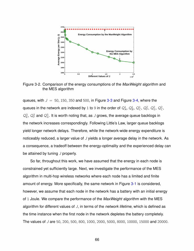
0 0.5 1 1.5 2 2.5
x 104
1800
1900
2000
2100
2200
2300
2400
2500
2600
2700
Different Values of J
Ave
rag
e E
ner
gy
per
Slo
t (µ
J) Energy Consumption by the MaxWeight Algorithm
Energy Consumption by the MES Algorithm
Figure 3-2. Comparison of the energy consumptions of the MaxWeight algorithm andthe MES algorithm
queues, with J = 50, 150, 350 and 500, in Figure 3-3 and Figure 3-4, where the
queues in the network are indexed by 1 to 9 in the order of Q1A, Q1B , Q1C , Q2F , Q2G , Q2C ,
Q3E , Q3F and Q3G . It is worth noting that, as J grows, the average queue backlogs in
the network increases correspondingly. Following Little’s Law, larger queue backlogs
yield longer network delays. Therefore, while the network-wide energy expenditure is
noticeably reduced, a larger value of J yields a longer average delay in the network. As
a consequence, a tradeoff between the energy-optimality and the experienced delay can
be attained by tuning J properly.
So far, throughout this work, we have assumed that the energy in each node is
constrained yet sufficiently large. Next, we investigate the performance of the MES
algorithm in multi-hop wireless networks where each node has a limited and finite
amount of energy. More specifically, the same network in Figure 3-1 is considered,
however, we assume that each node in the network has a battery with an initial energy
of 1 Joule. We compare the performance of the MaxWeight algorithm with the MES
algorithm for different values of J, in terms of the network lifetime, which is defined as
the time instance when the first node in the network depletes the battery completely.
The values of J are 50, 200, 500, 800, 1000, 2000, 5000, 8000, 10000, 15000 and 20000.
66
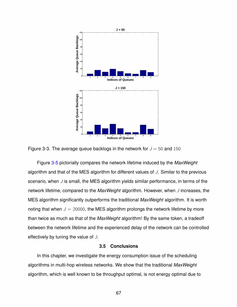
1 2 3 4 5 6 7 8 90
20
40
60
80
100
120
Indices of QueuesA
vera
ge
Qu
eue
Bac
klo
gs
J = 50
1 2 3 4 5 6 7 8 90
20
40
60
80
100
120
Indices of Queues
Ave
rag
e Q
ueu
e B
ackl
og
s
J = 150
Figure 3-3. The average queue backlogs in the network for J = 50 and 150
Figure 3-5 pictorially compares the network lifetime induced by the MaxWeight
algorithm and that of the MES algorithm for different values of J. Similar to the previous
scenario, when J is small, the MES algorithm yields similar performance, in terms of the
network lifetime, compared to the MaxWeight algorithm. However, when J increases, the
MES algorithm significantly outperforms the traditional MaxWeight algorithm. It is worth
noting that when J = 20000, the MES algorithm prolongs the network lifetime by more
than twice as much as that of the MaxWeight algorithm! By the same token, a tradeoff
between the network lifetime and the experienced delay of the network can be controlled
effectively by tuning the value of J.
3.5 Conclusions
In this chapter, we investigate the energy consumption issue of the scheduling
algorithms in multi-hop wireless networks. We show that the traditional MaxWeight
algorithm, which is well known to be throughput optimal, is not energy optimal due to
67

1 2 3 4 5 6 7 8 90
20
40
60
80
100
120
Indices of QueuesA
vera
ge
Qu
eue
Bac
klo
gs
J = 350
1 2 3 4 5 6 7 8 90
20
40
60
80
100
120
Indices of Queues
Ave
rag
e Q
ueu
e B
ackl
og
s
J = 500
Figure 3-4. The average queue backlogs in the network for J = 350 and 500
0 0.2 0.4 0.6 0.8 1 1.2 1.4 1.6 1.8 2
x 104
1500
2000
2500
3000
3500
4000
Different Values of J
Lif
etim
e o
f th
e N
etw
ork
Lifetime by the MaxWeight Algorithm
Lifetime Improvement by the MES Algorithm
Figure 3-5. Comparison of the lifetime of the MaxWeight algorithm and the MESalgorithm
the overlook of the energy consumptions induced by inevitable packet retransmissions.
In light of this, we propose a minimum energy scheduling (MES) algorithm which
significantly reduces the energy consumption compared to the original MaxWeight
algorithm. In addition, we analytically show that the MES algorithm is essentially energy
optimal in the sense that the average energy expenditure of the MES algorithm can be
68

pushed arbitrarily close to the global minimum solution. Moreover, the improvement on
the energy efficiency is achieved without losing the throughput-optimality. Therefore,
the proposed MES algorithm is of great importance for network protocol designs in
energy-constrained multi-hop wireless networks such as wireless sensor networks.
69
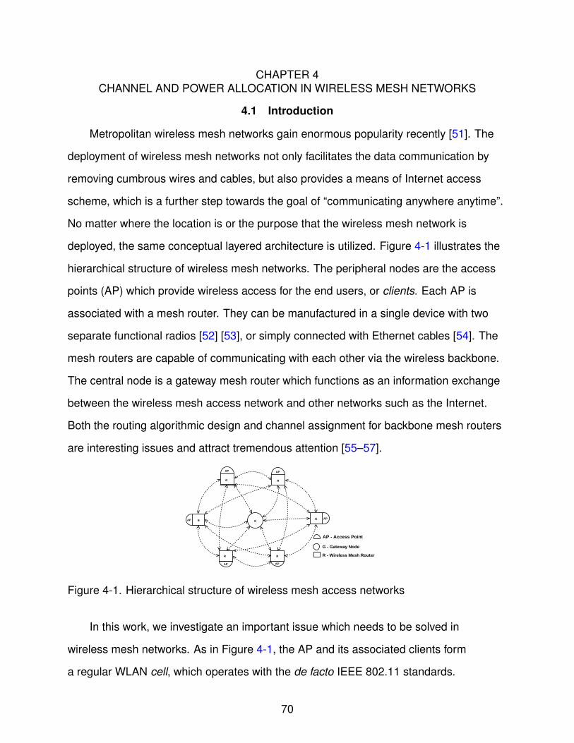
CHAPTER 4CHANNEL AND POWER ALLOCATION IN WIRELESS MESH NETWORKS
4.1 Introduction
Metropolitan wireless mesh networks gain enormous popularity recently [51]. The
deployment of wireless mesh networks not only facilitates the data communication by
removing cumbrous wires and cables, but also provides a means of Internet access
scheme, which is a further step towards the goal of “communicating anywhere anytime”.
No matter where the location is or the purpose that the wireless mesh network is
deployed, the same conceptual layered architecture is utilized. Figure 4-1 illustrates the
hierarchical structure of wireless mesh networks. The peripheral nodes are the access
points (AP) which provide wireless access for the end users, or clients. Each AP is
associated with a mesh router. They can be manufactured in a single device with two
separate functional radios [52] [53], or simply connected with Ethernet cables [54]. The
mesh routers are capable of communicating with each other via the wireless backbone.
The central node is a gateway mesh router which functions as an information exchange
between the wireless mesh access network and other networks such as the Internet.
Both the routing algorithmic design and channel assignment for backbone mesh routers
are interesting issues and attract tremendous attention [55–57].
AP
R
AP
R
AP
R
AP
AP R
R
APRG
AP - Access Point
G - Gateway Node
R - Wireless Mesh Router
Figure 4-1. Hierarchical structure of wireless mesh access networks
In this work, we investigate an important issue which needs to be solved in
wireless mesh networks. As in Figure 4-1, the AP and its associated clients form
a regular WLAN cell, which operates with the de facto IEEE 802.11 standards.
70
The throughput of one cell depends on the signal-to-interference-plus-noise ratio
(SINR) experienced at the receiver where the interference mainly comes from the
other operating cells. For example, if each of the cells operates with IEEE 802.11b
standard, we can utilize a different frequency band such as IEEE 802.11a or WiMAX
[58], for the inter-cell communication among mesh routers and hence causes no
interference to intra-cell transmissions. However, the co-channel interference from other
operating cells is inevitable due to the limitation of available transmission channels,
e.g., 3 non-overlapping channels in our example. Most current off-the-shelf APs are
capable of adjusting the transmission rate according to the measured channel condition
which is indicated by transmission bit error rate (BER). Given a particular modulation
scheme, BER is uniquely determined by the SINR experienced by the receiver of the
link. Generally speaking, higher SINR value yields lower BER and higher data rate.
Therefore, the mutual interference dramatically degrades the transmission rate of each
cell and the aggregated throughput of the whole network [59]. Each AP attempts to
tune the physical parameters such as operating frequency1 and transmission power in
order to maximize the SINR and hence the throughput. In our work, we investigate the
issue of maximizing the overall throughput of the network, defined as the summation
of throughput of all cells, by finding the optimal frequency and transmission power
allocation strategy. Also, due to the concern of scalability and computational complexity,
we prefer a decentralized solution to the throughput maximization problem.
Unfortunately, the throughput maximization problem is challenging. For example,
the frequency and power selected by one AP affects the SINR of other APs, and vice
versa. Worse yet, if the APs belong to different regulation entities, the non-cooperative
APs may only want to maximize their own cell’s throughput rather than the overall one.
Therefore, the throughput maximization problem is coupled and finding the optimum
1 We will use frequency and channel interchangeably.
71
solution is not straightforward. Moreover, traditional site-planning methods in cellular
networks are not feasible either. For example, the network administrator may want to
add more APs when more users are joining the network or disable some APs where
the associated users fail to pay the bill. The network topology is not static, although the
changes take place slowly. Therefore, the demand for adaptability and light computation
burden requires a decentralized solution for the throughput maximization problem.
In this work, we analyze the throughput maximization problem for both cooperative
and non-cooperative scenarios. In the cooperative case, we model the interaction
among all APs as an identical interest game and present a decentralized negotiation-based
throughput maximizing algorithm for the joint frequency and power assignment. We
show that this algorithm converges to the optimal frequency and power assignment
strategy, which maximizes the overall throughput of the wireless mesh access network,
with arbitrarily high probability. In the cases of non-cooperative APs, we prove the
existence of Nash equilibria and show that the overall throughput performance is usually
inferior to the cooperative cases. To bridge the performance gap, we propose a linear
pricing scheme to combat with the selfish behaviors of non-cooperative APs.
The rest of this chapter is organized as follows. Section 4.2 outlines the system
model we considered in the work. The cooperative wireless mesh access networks
and the non-cooperative counterpart are investigated in Section 4.3 and Section 4.4,
respectively. An extension of our model is discussed in Section 4.5 and the performance
evaluation is provided in Section 4.6. Finally, Section 4.7 concludes this chapter.
4.2 System Model
In this work, we consider a wireless mesh access network illustrated in Figure 4-1.
Each AP and corresponding clients form a cell. Without loss of generality, we assume
that all the cells operate with IEEE 802.11b standard and the interference exclusively
comes from the cells with same frequency. Furthermore, the distance between cells
are sufficiently large in the sense that the accumulated interference experienced at the
72
receiver only affects the SINR value and not block the whole transmission. We assume
that the channels are slow-varying additive white Gaussian noise (AWGN) channels.
The channel gains of each pair of nodes are assumed to be constant over the time
period of interest. As we are interested in the maximum achievable throughput, we
consider the worst case where all APs are saturated. In other words, the APs always
have packets to transmit and they can communicate with each other via the backbone
mesh routers with negligible delay. Also, we assume that the APs are transmitters and
clients are receivers due to the dominance of downlink traffic, as assumed2 in [61]
[62] and [63]. We only focus on the joint frequency and power allocation where the
contention behavior is less relevant and thus omitted. Therefore, we can simplify our
model as that all the APs are transmitting data to the associated clients consistently. We
assume that each AP is capable of adjusting the operating frequency and power as well
as acquiring the SINR values measured at the client by short ACK messages.
Let us first consider the simplest case where there is only one cell in the wireless
mesh access network, i.e., a single WLAN. In the following two sections, we assume
that the APs have pre-determined and fixed modulation and coding schemes. In other
words, upon receiving the SINR value3 measured by the client, denoted by γ, the AP
tunes the physical parameters in order to maximize the throughput, which is defined as
R∗(γ) = maxRiRi × (1− Pe(γ,Ri)) (4–1)
where Ri is the raw data rate specified by the IEEE 802.11 standard and R∗, i.e., the
throughput of this cell, is a non-decreasing function of received SINR γ. Pe is the error
2 The dominance of the downlink traffic is verified by the experimental measurementsin [60] as well.
3 Although there is no interference in this case, we adopt SINR instead of SNR fornotation consistency.
73
probability of the transmission channel, which is a function of SINR value providing the
modulation and coding scheme [64]. Apparently, if there is only one cell in the mesh
access network, the AP will boost the power as much as possible to increase the value
of γ and thus the throughput is maximized.
We now consider the cases where N cells coexist in the wireless mesh access
network. Let pi and fi denote the power and frequency for the i -th AP, respectively. We
use p = [p1, p2, · · · , pN ] and f = [f1, f2, · · · , fN ] to represent the power and frequency
assignment vector for all N APs. Therefore, for each cell i , the value of SINR4 , i.e., γi , is
a function of (p, f). The throughput of one cell depends not only on the power level and
frequency of itself, but also those of other APs in the network. Therefore, the throughput
maximization problem is coupled and by no means straightforward.
In the following two sections, we will discuss the scenarios where the APs are
cooperative and non-cooperative, respectively, under the assumption that the modulation
and coding schemes of APs are pre-loaded and fixed. In Section 4.5, we will extend our
analysis by considering the scenario where the APs are capable of adaptive coding and
modulation. The performance evaluation of all scenarios are provided by simulations in
Section 4.6.
4.3 Cooperative Access Networks
In this section, we consider the scenarios where all APs in the wireless mesh
access network are cooperative. The transmission power of APs are quantized into
discrete power levels for simplicity. From the system point of view, we want to find a joint
frequency and power level assignment such that the overall throughput in the whole
4 Throughout the chapter, the term SINR of the cell represents the average SINRamong all the clients in the cell, which can be obtained by a moving average of thereported SINR value.
74
network is maximized. Our objective function can be written as
Unetwork(p, f) =
N∑i=1
R∗i (γi) =
N∑i=1
R∗i (p, f) (4–2)
where R∗i is defined in (4–1).
However, finding the optimal frequency and power assignment which maximizes
(4–2) is non-trivial. The interdependency makes the problem coupled and difficult to
solve by traditional optimization methods [65]. A combination of (p, f) is named a profile
and a naive approach to solve the problem is to investigate all profiles exhaustively.
However, this is impossible in practice. For example, in a medium-size wireless mesh
access network with 20 APs where each has 3 frequency channels and 10 power levels,
the search space is (3 × 10)20 profiles! Obviously, the centralized algorithms are not
favorable in the wireless mesh access network due to the scalability concern. Next, we
will introduce a decentralized negotiation-based throughput maximization algorithm,
from a game-theoretical perspective.
4.3.1 Cooperative Throughput Maximization Game
The APs in the wireless mesh access networks are considered as players, i.e.,
decision makers of the game. We model the interaction among APs as a Cooperative
Throughput Maximization Game (CTMG), where each player has an identical objective
function Ui , as
Ui(p, f) = Unetwork(p, f) =
N∑j=1
R∗j (p, f) , ∀i . (4–3)
For each player i , all possible frequency and power level pairs form a strategy space
Φi which has a size of c × l , where c is the number of frequency channels available and
l is the number of feasible power levels. Define
Ω = Φ1 ×Φ2 × · · · ×ΦN . (4–4)
Then, the N players autonomously negotiate about the joint frequency-power profile
in Ω in order to find the optimal profile which maximizes (4–3). However, due to the
75
interdependency among N players caused by mutual interference, one question of
interest is that whether this negotiation will eventually meet an agreement, a.k.a., a
Nash equilibrium. The importance of Nash equilibria lies in that a possible steady state
of the system is guaranteed. If the game has no Nash equilibrium, the negotiation
process never stops and oscillates in an everlasting fashion. In addition, we are
concerning about what the performance of the steady states would be, if exist, in terms
of overall throughput of the whole network. We provide answers to these questions in
the following.
Lemma 3. The CTMG is a potential game.
A potential game is defined as a game where there exists a potential function P
such that
P(a′, a−i)− P(a′′, a−i) = Ui(a′, a−i)− Ui(a′′, a−i) ∀i , a′, a′′ (4–5)
where Ui is the utility function for player i and a′, a′′ are two arbitrary strategies in Φi .
More specifically, we have a′ = [p′i , f′i ] and a′′ = [p′′i , f
′′i ]. The notation of a−i denotes the
vector of choices made by all players other than i . Potential games have been broadly
applied in modeling the interactions in communication networks [66]. The popularity is
on account of the nice properties of potential games, such as
– Potential games have at least one Nash equilibrium.
– All Nash equilibria are the maximizers of the potential function, either locally orglobally.
– There are several learning schemes available which are guaranteed to converge toa Nash equilibrium, such as better response and best response [67] [68].
For detailed description about potential games, readers are referred to [67] and [69],
which investigate the potential game theory in engineering context.
We observe that in the cooperative case, each player has the same utility function
as in (4–3), which is the overall throughput of the network. Apparently, one potential
76

function of the game is the common utility function itself, i.e.,
P = U1 = U2 = · · · = UN . (4–6)
In fact, the games where all players share the same utility function are called identical
interest games [70], which is a special case of potential games and hence all the
properties of potential games can be applied directly.
In the literature, both best response and better response are popular learning
mechanisms that have been utilized in potential games [71–73]. At each step of the best
response approach, one of the players investigates its strategy space and chooses the
one with maximum utility value. This updating procedure is carried out sequentially. The
primary drawback of the best response is the computational complexity, which grows
linearly with the cardinality of the strategy space. An improvement of the best response
is the so-called better response, where at each step, the player updates as long as
the randomly selected strategy yields a better performance. The dramatically reduced
computation is the tradeoff with the convergence speed. Both the best response and the
better response dynamics are guaranteed to converge to a Nash equilibrium in potential
games [66]. However, there may be multiple Nash equilibria in a potential game and the
performance of different equilibria may vary dramatically. Therefore, although the best
response and the better response could guarantee the convergence, they may reach an
undesirable Nash equilibrium with inferior performance.
A DB C
1 2 12
1 2 21
Figure 4-2. An illustrative example of multiple Nash equilibria
Let us consider an illustrative example in Figure 4-2. There are four labeled APs
in the network. A and B are close to each other, and so are C and D. Without loss of
77
generality, we assume that the APs have the same power and only adjust the operating
frequencies in an order of A → B → C → D to avoid the interference. The adaptation
continues with the best response mechanism until a Nash equilibrium is reached.
Suppose that there are two frequency channels available, say 1 and 2. First, A randomly
selects one channel, say 1. B will pick 2. Next, C has the chance to update. Since C
is closer to B than A, channel 1 will be selected. Finally, D will choose channel 2. By
inspection, we claim that profile 1 − 2 − 2 − 1 is a Nash equilibrium since no player is
willing to update its strategy unilaterally. Meanwhile, we observe that another profile
1 − 2 − 1 − 2 is also a Nash equilibrium. Obviously, the second Nash equilibrium
generates much less interference than the first Nash equilibrium and hence yields
superior performance in terms of overall throughput. However, the best response only
leads to the less desirable Nash equilibrium.
In fact, the existence of multiple Nash equilibria is observed in [71] by simulations.
However, the authors fail to specify which one would be the steady state of their game
due to the limitation of the best response, even in a statistical fashion. Recall that
the Nash equilibria are the maximizers of the potential function in potential games,
converging to an inferior Nash equilibrium analogously indicates being trapped at a local
optimum of the potential function. However, it is the global optimum, i.e., the optimal
Nash equilibrium, that is the desirable steady state which we are yearning for.
Next, we introduce a negotiation-based throughput maximization algorithm
(NETMA) which can converge to the optimal Nash equilibrium with arbitrarily high
probability.
4.3.2 NETMA- Negotiation-Based Throughput Maximization Algorithm
We assume that the APs are homogeneous and each has a unique ID for routing
purpose. Each AP maintains two variables Dpre and Dcur . The AP has the knowledge of
its current throughput and records it in Dcur .Whenever there is a change of throughput
78

caused by exterior interference5 , the AP sets Dpre = Dcur and resets Dcur with the newly
measured throughput. When the wireless mesh access network enters the negotiation
phase6 , NETMA is executed. The detailed procedure of NETMA is provided as follows.
NETMA:
– Initialization: For each AP, a pair of frequency and power level is randomlyselected. Set Dpre = Dcur , the current throughput.
– Repeat:
1. Randomly choose one of the AP, say k , as the updating one, i.e., each APupdates with probability 1/N.
2. For the updating AP k :
(a) Randomly chooses a pair of frequency and power level, say f ′ andp′, from the strategy space Φk . Then the AP computes the currentthroughput with f ′ and p′ and records it into Dcur .
(b) Broadcasts a short notifying message which contains its unique IDk to allthe other APs in the mesh access network.
3. For each AP other than k , say j :
(a) If the γj value changes, records the previous throughput into Dpre and thecurrent throughput into Dcur . Remains unchanged otherwise.
(b) Upon receiving the notifying message, a three-value vector of [Dpre,Dcur , IDj ]is sent back to the k-th AP.
4. After receiving all the three-value vectors by counting the identifiers IDj , thek-th AP computes the sum throughput before and after f ′ and p′ are selected,which are denoted by Ppre and Pcur .
5 We assume the channel is slow-varying and the change of throughput for a singlecell is due to the mutual interference only.
6 To reduce the negotiation overhead, a negotiation phase can be initiated by thenetwork administrator after a new contracted user joins or a current user terminates theservice, or on a daily basis.
79
5. For a smoothing factor τ > 0, the k-th AP keeps f ′ and p′ with probability
ePcur/τ
ePcur/τ + ePpre/τ=
1
1 + e(Ppre−Pcur )/τ(4–7)
6. The k-th AP broadcasts another short notifying message, which indicates theend of updating process and a specific number δ, to all the other APs.
– Until: The stopping criteria Γ is met.
Note that in step 6, the specific format of δ depends on the predefined stopping
criterion Γ. For example,
• If the stopping criterion is the maximum number of negotiation steps, δ is a counterwhich adds one after each updating process.
• If the stopping criterion is that no AP has updated for a certain number of steps, δis a binary number where 1 means updating.
• If the stopping criterion is that the difference between sum throughput obtained inconsecutive steps are less than a predefined threshold ϵ, δ is the calculated sumthroughput after each updating process.
We can have other stopping criteria Γs and corresponding formats of δ as well.
The NETMA algorithm is inspired by the work in [74], where a similar algorithm
was first introduced in the context of stream control in MIMO interference networks. The
distinguishing feature of this type of negotiation algorithms, from the better response and
the best response, is the randomness deliberately introduced on the decision making in
step 5. The rationale can be illustrated in Figure 4-2 intuitively. If there is no randomness
in decision making , i.e., τ = 0, the four APs may get trapped at a low efficiency Nash
equilibrium 1− 2− 2− 1. However, with the randomness caused by nonzero τ , they may
reach an intermediate state 1 − 2 − 2 − 2 and arrive at the optimum Nash equilibrium
1 − 2 − 1 − 2 eventually. Moreover, the updating rule in step 5 also implies that if f ′ and
p′ yield a better performance, i.e., Ppre − Pcur < 0, the k-th AP will keep them with high
probability. Otherwise, it will change with high probability.
The steady state behavior of NETMA is characterized in the following theorem.
80
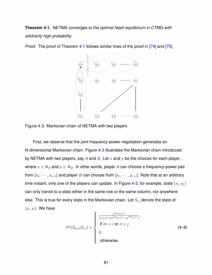
Theorem 4.1. NETMA converges to the optimal Nash equilibrium in CTMG with
arbitrarily high probability.
Proof. The proof of Theorem 4.1 follows similar lines of the proof in [74] and [75].
1 1,x y 1 2,x y 1 3,x y 1, c lx y ×
,c l c lx y× ×, 2c lx y× , 3c lx y×
2, 1x y
3, 1x y
, 1c lx y×
2, 2x y 2, 3x y 2, c lx y ×
Figure 4-3. Markovian chain of NETMA with two players
First, we observe that the joint frequency-power negotiation generates an
N-dimensional Markovian chain. Figure 4-3 illustrates the Markovian chain introduced
by NETMA with two players, say A and B. Let x and y be the choices for each player ,
where x ∈ ΦA and y ∈ ΦB . In other words, player A can choose a frequency-power pair
from [x1, · · · , xc×l ] and player B can choose from [y1, · · · , yc×l ]. Note that at an arbitrary
time instant, only one of the players can update. In Figure 4-3, for example, state (x1, y1)
can only transit to a state either in the same row or the same column, not anywhere
else. This is true for every state in the Markovian chain. Let Si ,j denote the state of
(xi , yi). We have
Pr(Sm,n|Si ,j) =
eP(Sm,n)/τ
2×c×l×(eP(Sm,n)/τ+eP(Si ,j )/τ ),
if m = i or n = j
0,
otherwise.
(4–8)
81
where τ is the smoothing factor in step 5 of NETMA and P(Si ,j) is the value of the
potential function, i.e., (4–21), at the state of Si ,j .
Let us derive the stationary distribution Pr ∗ for each state. We examine the
balanced equations. Writing the balance equations [76] at the dashed line, we obtain
c×l∑k=2
Pr ∗(S1,1)× Pr(S1,k |S1,1) =c×l∑k=2
Pr ∗(S1,k)× Pr(S1,1|S1,k). (4–9)
By substituting (4–9) with (4–8), we have
∑c×lk=2 Pr
∗(S1,1)× eP(S1,k )/τ
eP(S1,1)/τ+eP(S1,k )/τ
=∑c×lk=2 Pr
∗(S1,k)× eP(S1,1)/τ
eP(S1,1)/τ+eP(S1,k )/τ. (4–10)
Observing the symmetry of equation (4–10) as well as the Markovian chain, we
note that the set of equations in (4–10) are all balanced if for arbitrary state S in the
strategy space Ω, the stationary distribution is
Pr ∗(S) = KeP(S)/τ (4–11)
where K is a constant. By applying the probability conservation law [77] [76], we obtain
the stationary distribution for the Markovian chain as
Pr ∗(S) =eP(S)/τ∑Si∈Ω e
P(Si )/τ(4–12)
for arbitrary state S ∈ Ω.
In addition, we observe that the Markovian chain is irreducible and aperiodic.
Therefore, the stationary distribution given in (4–12) is valid and unique.
Let S∗ be the optimal state which yields the maximum value of potential function P,
i.e.,
S∗ = argmaxSi∈ΩP(Si). (4–13)
82
From (4–12), we have
limτ→0Pr ∗(S∗) = 1 (4–14)
which substantiates that NETMA converges to the optimal state in probability.
Finally, the analogous analysis can be straightforwardly extended to an N-dimensional
Markovian chain and thus completes the proof.
In NETMA, there is no central computational unit required. The joint frequency-power
assignment is achieved by negotiations among cooperative APs and the maximum
overall throughput is achieved with arbitrarily high probability. The autonomous behavior
and decentralized implementation make NETMA suitable for large scale wireless mesh
access networks. Moreover, NETMA has fast adaptability for the topology change of
the wireless mesh access networks. NETMA does not depend on any rate adaption
algorithms, nor on any underlying MAC protocols. In our simulation in Section 4.6, we
use IEEE 802.11b as the MAC layer protocol. However, it can be easily extended to
arbitrary MAC protocol with multi-rate multi-channel capability, such as IEEE 802.11a.
In addition, even with the existence of exterior interference source, such as coexisting
WLANs, NETMA works properly as well since the objective of NETMA is to maximize
the overall throughput of the network in the current wireless environments. The tradeoff
between algorithmic performance and convergence speed is controlled by parameter
τ in step 5, where large τ represents extensive space search with slow convergence.
On the contrary, small τ represents limited space search with fast convergence. Note
that the smoothing factor τ here is analogous to the concept of temperature in simulated
annealing [78]. Therefore, it is advisable that at the beginning period of the negotiation,
the value of τ is set with a large number and keeps deceasing as the negotiation
iterates. We choose τ = 10/k2 in our simulations, where k denotes the negotiation step.
In step 1, we require that each AP updates with a probability of 1/N. For example,
we can utilize a random token mechanism where each updating AP randomly selects
an AP as the next updating AP, i.e., passing the token. Note that in NETMA, even an
83
erroneous operation happens, for example, two APs update at the same time in our
case, it only prolongs the convergence time for NETMA yet does not affect the final
output of NETMA. This is because that such an error, as verified in [72] via extensive
simulations, has no influence on the statistically monotonic-increasing tendency of the
potential function.
4.4 Non-Cooperative Access Networks
In the previous section, we discuss the scenarios where all APs in the wireless
mesh access network are cooperative, and the overall throughput is maximized
by negotiations among autonomous APs using the NETMA mechanism. However,
cooperation is not always attainable. Although the functionality of relaying packets
for each other can be achieved by incentive mechanisms such as [79], the adjustable
parameters inside each cell cannot be enforced and effectively controlled. The N APs
may belong to distinct self-interested users and they care about exclusively their own
throughput rather than the overall aggregated throughput. In other words, the utility
function of each selfish user is
Ui = R∗i (γi) (4–15)
where R∗i is the throughput of the i -th cell, defined in (4–1). Analogous to CTMG, we
can formulate the interaction among N selfish APs as a Non-cooperative Throughput
Maximizing Game (NTMG) where each AP is attempting to find the frequency-power
pair which maximizes its own SINR value as well as the corresponding throughput. As in
the cooperative case, each player’s utility function depends on the frequency and power
of itself as well as those of others. However, NTMG is no longer an identical interest
game.
Lemma 4. In NTMG, all the APs will transmit with the maximal power at the Nash
equilibrium, if exists.
84
Proof. The proof of Lemma 4 is straightforward. For a single player, we have
γi =pigii∑
k∈Fi (fi ) pkgki + Ni. (4–16)
where gij is the channel gain from cell i ’s transmitter to j ’s receiver and Ni is the
Gaussian noise at the i ’s receiver. Fi(fi) denotes the set of cells which operate at
the same frequency fi other than cell i . Note that given other players’ strategies, γi
is a monotonic increasing function of pi and so is Ui . Assume at a Nash equilibrium
of NTMG, the k-th AP has a power level of pk satisfying 0 ≤ pk < pmax , where pmax
denotes the maximum power defined by MAC layer. The k-th AP is inclined to increase
its power pk in order to yield a higher value of Ui , which contradicts the definition of Nash
equilibrium. Thus, at the Nash equilibrium of NTMG, if exists, all the APs will operate at
the same power level, i.e., pmax .
Based on Lemma 4, the NTMG can be viewed as a simplified game where each
player has the same power and only adjusts the frequency to minimize the interference.
Moreover, according to (4–15) (4–16) and the assumption of uniform environment, the
NTMG is equivalent to the following simplified game where each player has the utility
function7 as
Ui = −(∑k∈Fi (fi )
pmaxgki + Ni) (4–17)
and Ui is a function of frequency assignment vector f exclusively.
As in the cooperative case, the frequency selection among N players is mutually
dependent. The question arises that whether this frequency adjusting dynamic
converges, or equivalently, whether NTMG has a Nash equilibrium. We provide the
answer of this question in the following theorem.
7 The negative sign comes from the convention that utility functions are the ones to bemaximized.
85

Theorem 4.2. There exists at least one Nash equilibrium in NTMG.
Proof. Let us first consider the simplified game. For each player, the utility function is
given as
Ui = −(∑k∈Fi (fi )
pkgki + Ni) (4–18)
= −(∑
k =i ,k∈N
pkgki × δ(fi − fk) + Ni) (4–19)
where
δ(k) =
1, if k = 0
0, otherwise.(4–20)
We conjecture that one of the feasible potential functions is
P = −12×∑i∈N
∑k∈Fi (fi )
pkgki . (4–21)
The verification is as follows.
2P = −∑i∈N
∑k∈Fi (fi )
pkgki
= −
∑k∈Fi (fi )
pkgki +∑j =i ,j∈N
∑k∈Fj (fj )
pkgkj
= −
∑k∈Fi (fi )
pkgki +∑j =i ,j∈N
pigijδ(fi − fj)
+∑
k∈Fj (fj ),k =i
pkgkj
= −
∑k =i ,k∈N
pkgkiδ(fk − fi)
+∑j =i ,j∈N
pigijδ(fi − fj)
+∑j =i ,j∈N
∑k∈Fj (fj ),k =i
pkgkj
. (4–22)
86

Note that
pkgkiδ(fk − fi) = pigikδ(fi − fk) (4–23)
for any pair of i , k . We have
P = −
∑k =i ,k∈N
pkgkiδ(fk − fi) +1
2×Q(−i)
(4–24)
where
Q(−i) =∑j =i ,j∈N
∑k∈Fi (fi ),k =i
pkgkj (4–25)
and Q(−i) is independent of fi . Therefore, for arbitrary two frequencies a′ and a′′ of
player i , we have
Qa′(−i) = Qa′′(−i) (4–26)
and
P(a′, a−i)− P(a′′, a−i)
=∑
k∈Fi (a′) pkgki +12×Qa′(−i)
−∑
k∈Fi (a′′) pkgki +12×Qa′′(−i)
= Ui(a
′, a−i)− Ui(a′′, a−i). (4–27)
Therefore, according to the definition in (4–5), the simplified game is a potential
game and has at least one Nash equilibrium. Thus, the existence of Nash equilibrium in
NTMG is obtained from the equivalence derived from Lemma 4.
As shown in Lemma 4, at the equilibrium, the non-cooperative APs will always
transmit at the maximum power level. This seem to be the best choice for each one of
the APs. However, it is usually not a favorable strategy from a social-welfare point of
view. To bridge the performance gap, we propose a linear pricing scheme to combat
with the selfish behaviors, i.e., the players are forced to pay a tax proportional to the
utilized resources. For example, we could impose a price to all selfish APs for the power
87
they utilize. Hence for each AP, the utility function becomes
Ui = R∗i (γi)− λippi (4–28)
where λip represents the power utilization price specific for the i -th AP and pi is its
transmission power. Therefore, the more power AP uses, the more tax it has to pay. By
imposing power prices properly, a more desirable equilibrium may be induced, from a
social-welfare point of view. We define the corresponding game as a Non-cooperative
Throughput Maximization Game with Pricing (NTMGP).
Let us first investigate the impact of prices on the behaviors of players. If λip = 0,
where no price is imposed, the i -th AP will transmit at the maximum power and causes
extra interference to other APs. However, if we impose an unbearably high price, say
λpi = ∞, the AP would rather not to transmit at all. Based on these observations,
we propose a heuristic linear pricing scheme to improve the overall throughput in
non-cooperative wireless mesh access networks.
To enforce the scheme, we introduce a pricing dictator unit (PDU) into the network
which determines the prices for all APs and informs them timely. In addition, we assume
that the PDU has the monitoring capability and is aware of the operating frequencies
of each cell. There are two prices charged by the PDU for each non-cooperative AP.
Besides the power utilizing price λip, a frequency switching price λif is imposed on the
i -th AP whenever it changes the operating frequency. The price setting process is
described as follows.
Price setting process:
Phase I:
– The PDU sets λ1f = · · ·λNf = 0 and λ1p = · · ·λNp = 0 and all APs play NTMGuntil converges, i.e., a Nash equilibrium is reached.
– The PDU collects the current throughput information from each cell, denotedby Mi , where i is the index of the cell.
88
Phase II:
– The PDU sets λ1f = · · ·λNf =∞.
– For each AP indexed by i = 1, · · · ,N :
1. The PDU sets λip = ∞ for the i -th AP and let the APs play the NTMGP.Upon convergence, the PDU collects the overall throughput, say Vi , in thecurrent price setting.
2. Calculate the power utilizing price for the i -th AP as
λip =Vi −
∑Nj=1,j =i Mj
pmax(4–29)
3. Reset λip = 0.
Output:
– Power utilizing price vector λp = [λ1p, · · · , λNp ]
– Frequency switching price vector λf = [∞, · · · ,∞]
In the price setting process above, the PDU imposes zero prices for all APs initially. As
a consequence, all APs will transmit with pmax at the equilibrium, as shown in Lemma
4. Upon convergence, the PDU fixes the frequency switching price to infinity which
discourages the non-cooperative APs from switching channels thereafter. In (4–29),∑Nj=1,j =i Mj is the sum throughput for all cells other than i , when the i -th AP transmits
with the maximal power due to the zero power price. Similarly, Vi is the sum throughput
of other cells when the i -th AP is silent due to the unaffordable power price. Therefore,
in (4–29), the power utilization price charged for the i -th AP, a.k.a., λip, can be viewed
as a compensation to the impact it causes on the overall throughput of other cells.
The more power it utilizes, the more severe it affects the other players and thus the
more it pays, as illustrated in (4–28). Hence, by imposing taxes deliberately, the selfish
behaviors of non-cooperative APs are effectively discouraged and a more desirable
equilibrium can be induced, in term of overall throughput of the whole network. The
proof of existence of Nash equilibrium in NTMGP is straightforward. Note that the utility
89

function of (4–28) is quasi-concave with respect to power. The existence of pure strategy
Nash equilibrium follows directly from the results of [80]. We will present the detailed
performance evaluation of CTMG, NTMG and NTMGP in Section 4.6.
4.5 An Extension to Adaptive Coding and Modulation Capable Devices
So far, we have assumed that the throughput of a cell is given in the form of (4–1),
which is not a continuous function. To be precise, in both Section 4.3 and Section 4.4,
we are confined to the traditional IEEE 802.11 family devices where the modulation
and coding schemes are pre-determined and fixed. For example, Table 4-1 provides
a mapping between SINR values and corresponding rates [81], the feasible data
transmission rate is a discrete set and is usually much less than the theoretical channel
capacity. We name such devices as legacy IEEE 802.11 devices.
Table 4-1. Data rates v.s. SINR thresholds with maximum BER = 10−5
Rate(Mbps) Minimum SINR (dB)1 -2.922 1.595.5 5.9811 6.99
However, thanks to the advance of coding techniques, the maximum data transmission
rate can be largely closed to the theoretical Shannon capacity in AWGN channels
[82]. Note that achieving this requires variable-rate transmissions by matching to the
instantaneous SINR, which can be implemented in practice through adaptive coding
and modulation (ACM) techniques [83]. This motivates us to extend our results to
ACM-capable devices. More specifically, we are considering more advanced and
powerful APs which attempt to tune the frequency and power in order to maximize
Ci(γi) =Wi log2(1 + γi) (4–30)
90
where Ci is the Shannon capacity of the i -th cell, andWi is the bandwidth. Note that in
this scenario, the maximum achievable transmission rate, as denoted by the Shannon
capacity, is a continuous variable with respect to γi , rather than discrete, as exemplified
in Table 4-1. It is worth noting that the only difference in this scenario is the alternative
objective function of each AP. Therefore, all the results we have obtained so far are
extendable8 to this special scenario with merely a change of the objective function.
Furthermore, due to the continuity of the objective function in (4–30), the aforementioned
heuristic pricing scheme in Section 4.4 can be improved. Without loss of generality, we
assume that all the cells have unity bandwidth. Restated, we assume that the PDU
is a centralized device which knows the channel environment sufficiently by greedy
acquiring. In addition, the PDU is assumed to have monitoring capability and is aware of
the operating frequency of each cell. The tailored pricing scheme for this ACM-capable
scenario is described as follows.
• First, the PDU sets λ1f = · · ·λNf = 0 and λ1p = · · ·λNp = 0 and all APs play selfishly,until a Nash equilibrium is achieved.
• The PDU sets λ1f = · · ·λNf =∞.
• For each AP indexed by i = 1, · · · ,N, the PDU sets
8 More specifically, in the cooperative case, we replace (4–2) with Unetwork(p, f) =∑Ni=1 Ci(γi) whereas in the non-cooperative case, (4–15) and (4–28) are replaced by
Ui = Ci(γi) and Ui = Ci(γi)− λippi , respectively.
91

λip = |∑k∈Fi
∂Ck∂pi
|
= |∑k∈Fi
− pk × gkk × gikln 2× (1 + γk)× (
∑j∈Fk pj × gjk + Nk)
2|
=∑k∈Fi
pk × gkk × gikln 2× (1 + γi)× (pk×gkkγk
)2
=∑k∈Fi
gik × γ2kln 2× (1 + γk)× pk × gkk
. (4–31)
Then the PDU informs each AP the corresponding prices, i.e., λif =∞ and λip calculated
in (4–31).
Note that the major difference in this pricing scheme lies in (4–31), where the λip
charged for the i -th AP is the Pigouvian price levied to discourage its reckless power
increase.
After obtaining the prices imposed by the PDU, each AP fixes the operating
frequency and calculates the optimum power p∗i , which maximizes Ui = Ci − piλip,
according to the following steps.
∂Ui∂pi=∂Ci∂pi
− λip (4–32)
where∂Ci∂pi=
giiln 2× (
∑k∈Fi pk × gki + Ni)× (1 + γi)
. (4–33)
By setting (4–32) equal to zero, we have
p∗i =
[1
ln 2× λip−∑k∈Fi pk × gki + Ni
gii
]pmaxpmin
. (4–34)
where [x ]ba denotes maxminb, x, a and pmax , pmin represent the maximum and
minimum power of the device, respectively. Note that∑k∈Fi pk × gki + Ni can be easily
measured when the i -th AP sets its transmission power to zero. Therefore, finding the
92
optimum power of each AP requires only local information and can be implemented in a
distributed fashion.
In (4–31), we observe that the prices imposed on APs depend on the power vector
p, and vice versa. Therefore, after each AP optimizes its power according to (4–34),
the PDU measures the new value of power, adjusts the price following (4–31), and then
announces the new price again. The pricing setting process in (4–31) and the utility
maximization process in (4–34) are executed in an iterative manner, until convergence.
The whole pricing scheme is summarized as follows.
Pricing Scheme:
1. The PDU initially sets zero prices. As a consequence, all APs will converge at aNash equilibrium with maximum power.
2. The PDU sets infinity for the frequency switching price which prevents the wholenetwork from unstable frequency oscillations.
3. The PDU sets and announces the power prices for each AP according to (4–31).
4. Informed by the PDU, each AP optimizes its transmission power following (4–34).
5. Go back to step 3 until the iteration converges.
The performance evaluation of this tailored pricing scheme is illustrated in the next
section.
4.6 Performance Evaluation
4.6.1 Legacy IEEE 802.11 Devices
In this subsection, we first investigate the performance of NETMA, NTMG and
NTMGP with legacy devices, i.e., the scenarios we considered in Section 4.3 and
Section 4.4. We assume the wireless mesh access network has N homogeneous APs.
The other simulation parameters are summarized as follows.
• Each AP has a maximum power pmax = 100mW and a minimum power pmin =10mW and 10 different power levels as [10mW , 20mW , · · · , 100mW ].
• The noise experienced at each receiver is assumed identical and has a power of2mW .
93
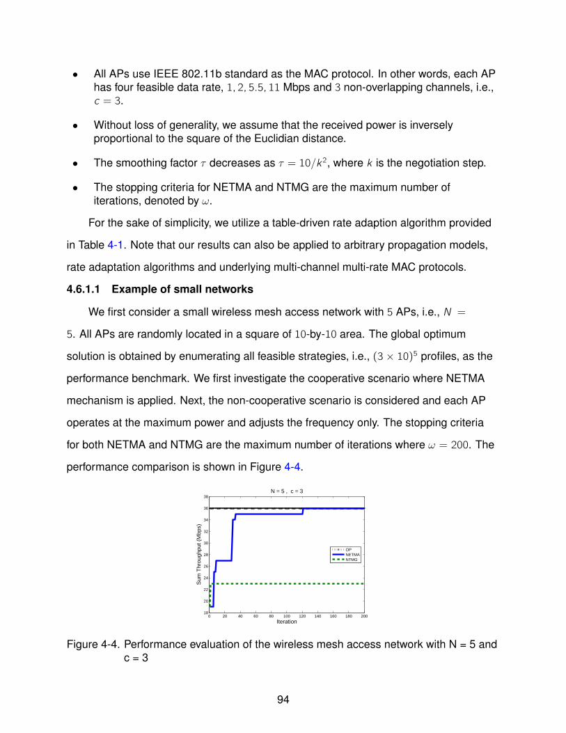
• All APs use IEEE 802.11b standard as the MAC protocol. In other words, each APhas four feasible data rate, 1, 2, 5.5, 11 Mbps and 3 non-overlapping channels, i.e.,c = 3.
• Without loss of generality, we assume that the received power is inverselyproportional to the square of the Euclidian distance.
• The smoothing factor τ decreases as τ = 10/k2, where k is the negotiation step.
• The stopping criteria for NETMA and NTMG are the maximum number ofiterations, denoted by ω.
For the sake of simplicity, we utilize a table-driven rate adaption algorithm provided
in Table 4-1. Note that our results can also be applied to arbitrary propagation models,
rate adaptation algorithms and underlying multi-channel multi-rate MAC protocols.
4.6.1.1 Example of small networks
We first consider a small wireless mesh access network with 5 APs, i.e., N =
5. All APs are randomly located in a square of 10-by-10 area. The global optimum
solution is obtained by enumerating all feasible strategies, i.e., (3 × 10)5 profiles, as the
performance benchmark. We first investigate the cooperative scenario where NETMA
mechanism is applied. Next, the non-cooperative scenario is considered and each AP
operates at the maximum power and adjusts the frequency only. The stopping criteria
for both NETMA and NTMG are the maximum number of iterations where ω = 200. The
performance comparison is shown in Figure 4-4.
0 20 40 60 80 100 120 140 160 180 20018
20
22
24
26
28
30
32
34
36
38
Iteration
Sum
Thr
ough
put (
Mbp
s)
N = 5 , c = 3
OPNETMANTMG
Figure 4-4. Performance evaluation of the wireless mesh access network with N = 5 andc = 3
94
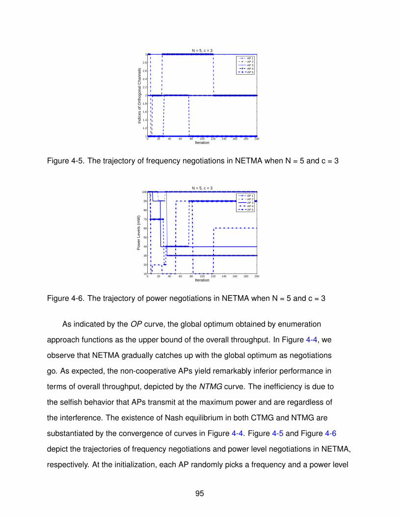
0 20 40 60 80 100 120 140 160 180 2001
1.2
1.4
1.6
1.8
2
2.2
2.4
2.6
2.8
3
IterationIn
dice
s of
Ort
hogo
nal C
hann
els
N = 5, c = 3
AP 1AP 2AP 3AP 4AP 5
Figure 4-5. The trajectory of frequency negotiations in NETMA when N = 5 and c = 3
0 20 40 60 80 100 120 140 160 180 20010
20
30
40
50
60
70
80
90
100
Iteration
Pow
er L
evel
s (m
W)
N = 5, c = 3
AP 1AP 2AP 3AP 4AP 5
Figure 4-6. The trajectory of power negotiations in NETMA when N = 5 and c = 3
As indicated by the OP curve, the global optimum obtained by enumeration
approach functions as the upper bound of the overall throughput. In Figure 4-4, we
observe that NETMA gradually catches up with the global optimum as negotiations
go. As expected, the non-cooperative APs yield remarkably inferior performance in
terms of overall throughput, depicted by the NTMG curve. The inefficiency is due to
the selfish behavior that APs transmit at the maximum power and are regardless of
the interference. The existence of Nash equilibrium in both CTMG and NTMG are
substantiated by the convergence of curves in Figure 4-4. Figure 4-5 and Figure 4-6
depict the trajectories of frequency negotiations and power level negotiations in NETMA,
respectively. At the initialization, each AP randomly picks a frequency and a power level
95
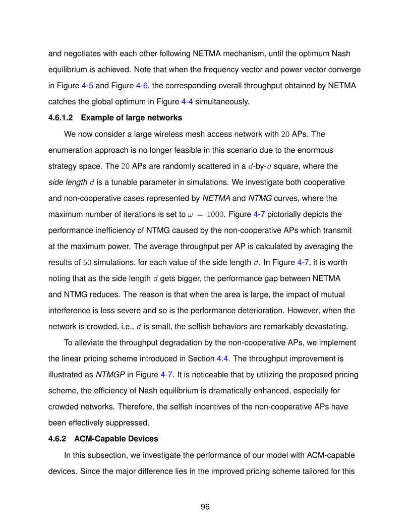
and negotiates with each other following NETMA mechanism, until the optimum Nash
equilibrium is achieved. Note that when the frequency vector and power vector converge
in Figure 4-5 and Figure 4-6, the corresponding overall throughput obtained by NETMA
catches the global optimum in Figure 4-4 simultaneously.
4.6.1.2 Example of large networks
We now consider a large wireless mesh access network with 20 APs. The
enumeration approach is no longer feasible in this scenario due to the enormous
strategy space. The 20 APs are randomly scattered in a d-by-d square, where the
side length d is a tunable parameter in simulations. We investigate both cooperative
and non-cooperative cases represented by NETMA and NTMG curves, where the
maximum number of iterations is set to ω = 1000. Figure 4-7 pictorially depicts the
performance inefficiency of NTMG caused by the non-cooperative APs which transmit
at the maximum power. The average throughput per AP is calculated by averaging the
results of 50 simulations, for each value of the side length d . In Figure 4-7, it is worth
noting that as the side length d gets bigger, the performance gap between NETMA
and NTMG reduces. The reason is that when the area is large, the impact of mutual
interference is less severe and so is the performance deterioration. However, when the
network is crowded, i.e., d is small, the selfish behaviors are remarkably devastating.
To alleviate the throughput degradation by the non-cooperative APs, we implement
the linear pricing scheme introduced in Section 4.4. The throughput improvement is
illustrated as NTMGP in Figure 4-7. It is noticeable that by utilizing the proposed pricing
scheme, the efficiency of Nash equilibrium is dramatically enhanced, especially for
crowded networks. Therefore, the selfish incentives of the non-cooperative APs have
been effectively suppressed.
4.6.2 ACM-Capable Devices
In this subsection, we investigate the performance of our model with ACM-capable
devices. Since the major difference lies in the improved pricing scheme tailored for this
96
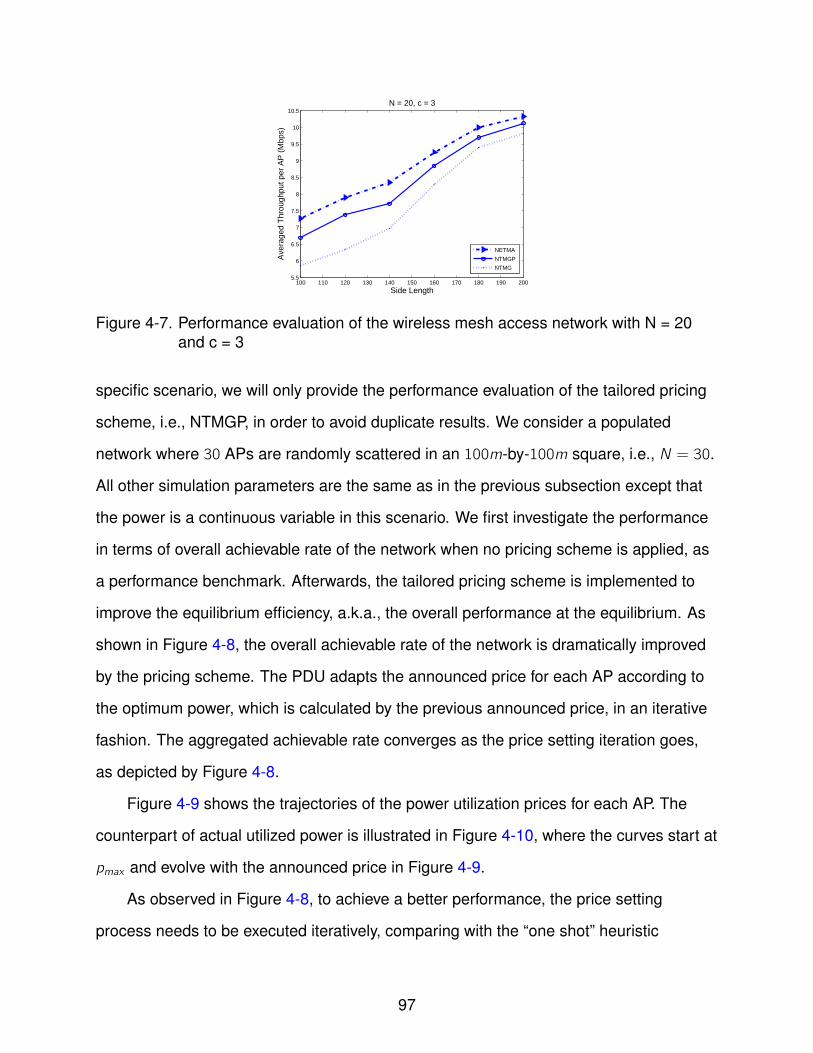
100 110 120 130 140 150 160 170 180 190 2005.5
6
6.5
7
7.5
8
8.5
9
9.5
10
10.5
Side LengthA
vera
ged
Thr
ough
put p
er A
P (
Mbp
s)
N = 20, c = 3
NETMA
NTMGP
NTMG
Figure 4-7. Performance evaluation of the wireless mesh access network with N = 20and c = 3
specific scenario, we will only provide the performance evaluation of the tailored pricing
scheme, i.e., NTMGP, in order to avoid duplicate results. We consider a populated
network where 30 APs are randomly scattered in an 100m-by-100m square, i.e., N = 30.
All other simulation parameters are the same as in the previous subsection except that
the power is a continuous variable in this scenario. We first investigate the performance
in terms of overall achievable rate of the network when no pricing scheme is applied, as
a performance benchmark. Afterwards, the tailored pricing scheme is implemented to
improve the equilibrium efficiency, a.k.a., the overall performance at the equilibrium. As
shown in Figure 4-8, the overall achievable rate of the network is dramatically improved
by the pricing scheme. The PDU adapts the announced price for each AP according to
the optimum power, which is calculated by the previous announced price, in an iterative
fashion. The aggregated achievable rate converges as the price setting iteration goes,
as depicted by Figure 4-8.
Figure 4-9 shows the trajectories of the power utilization prices for each AP. The
counterpart of actual utilized power is illustrated in Figure 4-10, where the curves start at
pmax and evolve with the announced price in Figure 4-9.
As observed in Figure 4-8, to achieve a better performance, the price setting
process needs to be executed iteratively, comparing with the “one shot” heuristic
97
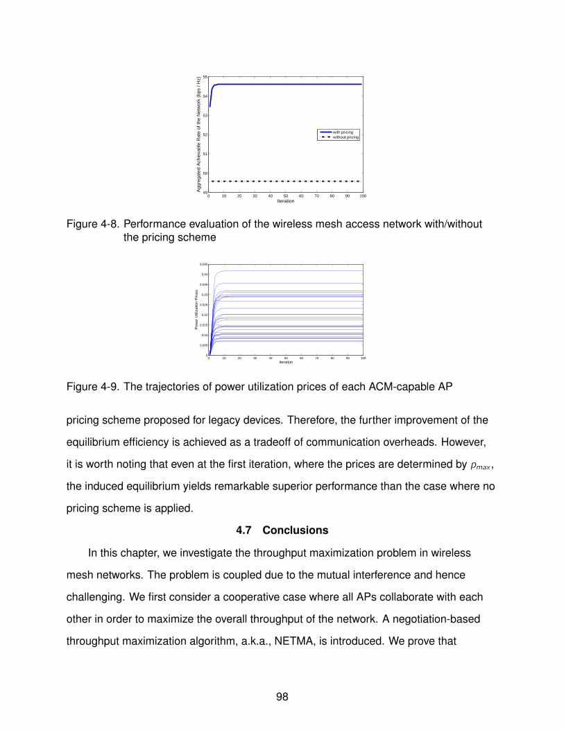
0 10 20 30 40 50 60 70 80 90 10049
50
51
52
53
54
55
IterationA
ggre
gate
d A
chie
vabl
e R
ate
of th
e N
etw
ork
(bps
/ H
z)
with pricingwithout pricing
Figure 4-8. Performance evaluation of the wireless mesh access network with/withoutthe pricing scheme
0 10 20 30 40 50 60 70 80 90 1000
0.005
0.01
0.015
0.02
0.025
0.03
0.035
0.04
0.045
Iteration
Pow
er U
tiliz
atio
n P
rices
Figure 4-9. The trajectories of power utilization prices of each ACM-capable AP
pricing scheme proposed for legacy devices. Therefore, the further improvement of the
equilibrium efficiency is achieved as a tradeoff of communication overheads. However,
it is worth noting that even at the first iteration, where the prices are determined by pmax ,
the induced equilibrium yields remarkable superior performance than the case where no
pricing scheme is applied.
4.7 Conclusions
In this chapter, we investigate the throughput maximization problem in wireless
mesh networks. The problem is coupled due to the mutual interference and hence
challenging. We first consider a cooperative case where all APs collaborate with each
other in order to maximize the overall throughput of the network. A negotiation-based
throughput maximization algorithm, a.k.a., NETMA, is introduced. We prove that
98

0 10 20 30 40 50 60 70 80 90 10010
20
30
40
50
60
70
80
90
100
Iteration
Act
ual U
tiliz
ed P
ower
(m
W)
Figure 4-10. The trajectories of actual power utilized by each ACM-capable AP
NETMA converges to the optimum solution with arbitrarily high probability. For the
non-cooperative scenarios, we show the existence and the inefficiency of Nash equilibria
due to the selfish behaviors. To bridge the performance gap, we propose a pricing
scheme which tremendously improves the performance in terms of overall throughput.
The analytical results are verified by simulations. In addition, we extend our model
and analytical results to the scenarios where more advanced APs are utilized, i.e., the
devices with the adaptive coding and modulation capability. In this scenario, we propose
a tailored pricing scheme which remarkably improves the overall performance in an
iterative fashion.
99
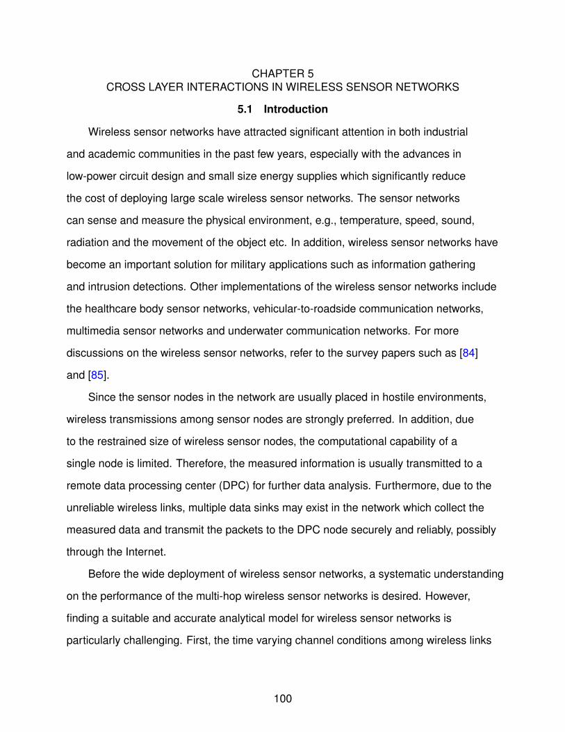
CHAPTER 5CROSS LAYER INTERACTIONS IN WIRELESS SENSOR NETWORKS
5.1 Introduction
Wireless sensor networks have attracted significant attention in both industrial
and academic communities in the past few years, especially with the advances in
low-power circuit design and small size energy supplies which significantly reduce
the cost of deploying large scale wireless sensor networks. The sensor networks
can sense and measure the physical environment, e.g., temperature, speed, sound,
radiation and the movement of the object etc. In addition, wireless sensor networks have
become an important solution for military applications such as information gathering
and intrusion detections. Other implementations of the wireless sensor networks include
the healthcare body sensor networks, vehicular-to-roadside communication networks,
multimedia sensor networks and underwater communication networks. For more
discussions on the wireless sensor networks, refer to the survey papers such as [84]
and [85].
Since the sensor nodes in the network are usually placed in hostile environments,
wireless transmissions among sensor nodes are strongly preferred. In addition, due
to the restrained size of wireless sensor nodes, the computational capability of a
single node is limited. Therefore, the measured information is usually transmitted to a
remote data processing center (DPC) for further data analysis. Furthermore, due to the
unreliable wireless links, multiple data sinks may exist in the network which collect the
measured data and transmit the packets to the DPC node securely and reliably, possibly
through the Internet.
Before the wide deployment of wireless sensor networks, a systematic understanding
on the performance of the multi-hop wireless sensor networks is desired. However,
finding a suitable and accurate analytical model for wireless sensor networks is
particularly challenging. First, the time varying channel conditions among wireless links
100
significantly complicate the analysis for the network performance in terms of throughput
and experienced delay, even in an average sense [1, 86, 87]. Secondly, due to the
unpredictability of the behavior of the monitored object, the exogenous traffic arrival
to the network, i.e., the number of newly generated packets, is a stochastic process.
Therefore, to ensure the stability of the network, i.e., to keep the queues in the network
constantly finite, the analytical model of wireless sensor networks should comprise a
rate admission control mechanism which can dynamically adjust the number of admitted
packets into the network. Thirdly, due to the hostile wireless communication links, a
dynamic routing scheme should be included in the analytical model. Moreover, the
model should capture the complex issue of wireless link scheduling which is significantly
challenging due to the mutual interference of wireless transmissions. Lastly, in order
to fully explore the network resource and to mitigate the network congestion, an
appropriate analytical network model should be able to dynamically deliver packets
through multiple data sinks and thus an automatic load balancing solution can be
achieved.
In the existing literature, most of the proposed models for wireless sensor networks
rely on the fluid model [6], where a flow is characterized by a source node and a
specific destination node, e.g., [3, 4, 6, 7]. However, this model is not applicable to the
cases where the generated packets can be delivered to any of the sink nodes, i.e., the
destination node is one of the sinks and is selected dynamically. Moreover, this fluid
model neglects the actual queue interactions within the wireless sensor network. In this
work, to study the cross layer interactions of the multi-hop wireless sensor networks, we
propose a constrained queueing model where a packet needs to wait for service in a
data queue. More specifically, we investigate the joint rate admission control, dynamic
routing, adaptive link scheduling and automatic load balancing solution to the wireless
sensor network through a set of interconnected queues. Due to the wireless interference
and the underlying scheduling constraints, at a particular time slot, only a subset
101
of queues can be scheduled for transmissions simultaneously. To demonstrate the
effectiveness of the proposed constrained queueing model, we investigate the stochastic
network utility maximization (SNUM) problem in multi-hop wireless sensor networks.
Based on the proposed queueing model, we develop an adaptive network resource
allocation (ANRA) scheme which is a cross layer solution to the SNUM problem and
yields a (1 − ϵ) near-optimal solution to the global optimum network utility where
ϵ > 0 can be arbitrarily small. The proposed ANRA scheme consists of multiple layer
components such as joint rate admission control, traffic splitting, dynamic routing as
well as adaptive link scheduling. In addition, the ANRA scheme is essentially an online
algorithm which only requires the instantaneous information of the current time slot and
hence significantly reduces the computational complexity.
The rest of the chapter is organized as follows. Section 5.2 briefly summarizes
the related work in the literature. The constrained queueing model for the cross layer
interactions of wireless sensor networks is proposed in Section 5.3. The stochastic
network utility maximization problem of the wireless sensor network is investigated in
Section 5.4, where a cross layer solution, a.k.a., the ANRA scheme is developed. The
performance analysis of the ANRA scheme is provided in Section 5.5. An example
which demonstrates the effectiveness of the ANRA scheme is given in Section 5.6 and
Section 5.7 concludes this chapter.
5.2 Related Work
To capture the cross layer interactions of multi-hop wireless sensor networks,
several analytical models have been proposed in the literature. For example, in [3–7,
88], the multi-hop network resource allocation problem has been studied through a fluid
model. Each flow, or session, is characterized by a source and a destination node where
single path routing or multi-path routing schemes are implemented. Most of the work
rely on the dual optimization framework which decomposes the complex cross layer
interactions into separate sub-layer problems by introducing dual variables. For example,
102
the flow injection rate, controlled by the source node of the flow, is calculated by solving
an optimization problem with the knowledge of the dual variables, a.k.a., shadow prices
[6, 7], of all the links that are utilized. However, there are several drawbacks for the fluid
based model. First, to calculate the optimum flow injection rate, the information along all
paths should be collected in order to implement the rate admission control mechanism.
In a dynamic environment such as wireless sensor networks, this process of information
collection may take a significant amount of time which inevitably prolongs the network
delay. Secondly, the optimization based solutions usually pursue fixed operating points
which are hardly optimal in dynamic wireless settings with stochastic traffic arrivals
and time varying channel conditions. Thirdly, the fluid model usually assumes that
the changes of the flow injection rates are “perceived” by all the nodes along its paths
instantaneously. The actual queue dynamics and interactions are neglected.
In contrast, following the seminal paper of [12], many solutions have been focused
on the queueing model for studying the complex interactions of communication
networks. Neely et.al. extend the results of [12] into wireless networks with time
varying channel conditions. For a more complete survey of this area, refer to [17].
The key component of the queue based solutions in these papers is the MaxWeight
scheduling algorithm [12, 14]. Intuitively, at a time slot, the network picks the set of
queues which (1) can be active simultaneously and (2) have the maximum overall
weight. It is well-known that the MaxWeight algorithm is throughput-optimal in the sense
that any arrival rate vector that can be supported by the network can be stabilized
under the MaxWeight scheduling algorithm. In addition, the MaxWeight algorithm is
an online policy which requires only the information about current queue sizes and
channel conditions. However, one notorious drawback of the MaxWeight algorithm is
the delay performance. The reason is that in order to achieve the throughput-optimality,
the MaxWeight algorithm explores a dynamic routing solution where long paths are
utilized even under a light traffic load. This phenomenon is substantiated via simulations
103

by [89]. In [89], the authors propose a variant of the MaxWeight algorithm where
the average number of hops of transmissions is minimized. Therefore, when the
traffic is light, the proposed solution provides a much lower delay than the traditional
MaxWeight algorithm. However, as a tradeoff, the induced network capacity region in
[89] is noticeably smaller than that of the original MaxWeight algorithm. Consequently,
it is difficult to provide a minimum rate guarantee on all the sessions in the network.
Our work is inspired by [89]. With respect to [89], however, our work innovates in the
following ways. First, different from [89], we focus on a heavy-loaded wireless sensor
network. Therefore, our solution incorporates a rate admission control mechanism
which is not considered in [89]. Secondly, rather than minimizing the overall number
of hops, we maximize the overall network utility which can also ensure the fairness
among competitive traffic sessions. Thirdly, we specifically provide a minimum average
rate guarantee for every session to ensure the QoS requirement. Fourthly, instead of a
single destination scenario as considered in [89], we extend the model to cases where
multiple data sink nodes are available. Each source node can deliver the packets to any
of the sinks. Moreover, the dynamic routing and the issue of automatic load balancing
is realized by the network on the fly. Finally, while [89] treats different sessions equally
when minimizing the overall number of hops, our model prioritizes all the sessions
with different QoS requirements. Therefore, a more flexible solution with service
differentiations can be achieved. We will present the constrained queueing model in
the next section.
5.3 A Constrained Queueing Model for Wireless Sensor Networks
5.3.1 Network Model
We consider a multi-hop wireless sensor network represented by a directed graph
G = N,L where N and L denote the set of vertices and the set of links, respectively.
We will use the notation of |A| to represent the cardinality of set A, e.g., the number
of nodes in the network is |N| and |L| is the number of links. The time is slotted as
104
t = 0, 1, · · · and at a particular time slot t, the instantaneous channel data rate of link
(m, n) ∈ L is denoted by µm,n(t). In other words, link (m, n) can transmit a number of
µm,n(t) packets during time slot t. Note that the value of µm,n(t) is a random variable.
Denote µµµ(t) as the network link rate vector at time slot t. In this work, we assume
that µµµ(t) remains constant within one time slot but is subject to changes at time slot
boundaries. The value of µµµ(t) is assumed to be evolving following an irreducible and
aperiodic Markovian chain with arbitrarily large yet finite number of states. However, the
steady state distributions are unknown to the network.
At time slot t, the network selects a feasible link schedule, denoted by I (t) =
I1(t), I2(t), · · · , I|L|(t) where Il(t) = 1 if link l is selected to be active and Il(t) = 0
otherwise. The set of all feasible link schedules is denoted by Ω(t) which is determined
by the underlying scheduling constraints such as interference models and duplex
constraints. Therefore, selecting an interference-free link schedule in the network graph
G is equivalent to the process of attaining an independent set in the associated conflict
graph G, where the vertices are the links in G and a link exists in G if the two original
links in G cannot transmit simultaneously.
5.3.2 Traffic Model
There are a number of |S | source nodes in the wireless sensor network which
consistently monitor the surroundings and inject exogenous traffic to the network. The
generated packets need to be delivered to the remote data processing center (DPC) in a
multi-hop fashion. To simplify analysis, we assume that each source node is associated
uniquely with a session. The set of source nodes is denoted by S = n01, n02, · · · , n0|S|
where n0s , s = 1, · · · , |S | is the source node of session s. It is worth noting that the
following analysis can be extended straightforwardly to the scenarios where each source
node may generate multiple sessions.
There are |D| number of sinks in the network which are connected to the remote
data processing center via the Internet. In other words, the sink nodes can be
105
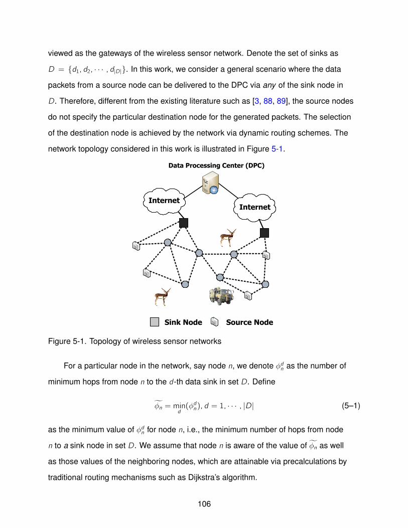
viewed as the gateways of the wireless sensor network. Denote the set of sinks as
D = d1, d2, · · · , d|D|. In this work, we consider a general scenario where the data
packets from a source node can be delivered to the DPC via any of the sink node in
D. Therefore, different from the existing literature such as [3, 88, 89], the source nodes
do not specify the particular destination node for the generated packets. The selection
of the destination node is achieved by the network via dynamic routing schemes. The
network topology considered in this work is illustrated in Figure 5-1.
Sink Node Source Node
InternetInternet
Data Processing Center (DPC)
Figure 5-1. Topology of wireless sensor networks
For a particular node in the network, say node n, we denote ϕdn as the number of
minimum hops from node n to the d-th data sink in set D. Define
ϕn = mind(ϕdn), d = 1, · · · , |D| (5–1)
as the minimum value of ϕdn for node n, i.e., the minimum number of hops from node
n to a sink node in set D. We assume that node n is aware of the value of ϕn as well
as those values of the neighboring nodes, which are attainable via precalculations by
traditional routing mechanisms such as Dijkstra’s algorithm.
106
At time slot t, the exogenous arrival of session s, i.e., the number of new packets1
generated by the source node of session s , is denoted by As(t). We assume that there
is an upper bound for the number of new packets within one time slot, i.e., As(t) ≤
Amax,∀s, t. For ease of exposition, we assume that As(t) is i.i.d. over time slots with an
average rate of λs . However, the data rates from multiple source nodes can be arbitrarily
correlated. For example, if the wireless sensor network is deployed for monitoring
purpose, it is very likely that a movement of the object will trigger several concurrent
updates of the nearby sensors.
Denote the vector λλλ = λ1, · · · ,λ|S| as the network arrival rate vector. The network
capacity region Λ is thus defined as all the feasible2 network arrival vectors that can
be supported by the network via certain policies, including those with the knowledge
of futuristic traffic arrivals and channel rate conditions. In this work, we consider a
heavy-loaded traffic scenario where the network arrival vector λλλ is outside of the network
capacity region. Therefore, in order to achieve the network stability, a rate admission
control mechanism is implemented at the source nodes. More specifically, at time slot
t, we only admit a number of Xs(t) packets into the network from the source node of
session s, i.e., n0s . Apparently, we have
Xs(t) ≤ As(t),∀s, t. (5–2)
In addition, we assume that each session has a continuous, concave and differentiable
utility function, denoted by Us(Xs(t)), which reflects the degree of satisfaction by
1 We assume that the packets have a fixed length. For scenarios with variable packetlengths, the unit of data transmissions can be changed to bits per slot and the followinganalysis still holds.
2 Note that additional constraints may be imposed. For example, the constraintson the minimum average rate and the maximum average power expenditure can beenforced. For more discussions, please refer to [17].
107
transmitting Xs(t) number of packets. It is worth noting that by selecting proper utility
functions, the fairness among competitive sessions can be achieved. For example, if
Us(Xs(t)) = log(Xs(t)), a proportional fairness among multiple sessions can be enforced
[4, 10, 11].
5.3.3 Queue Management
For each node n in the network, there are |N| − ϕn number of queues that are
maintained and updated. The queues are denoted by Qn,h, where h = ϕn, · · · , |N| − 1.
Note that |N| − 1 is the maximum number of hops for a loop-free routing path in the
network. The packets in the queue of Qn,h are guaranteed to reach one of the sink
nodes in set D within h hops, as will be shown in Section 5.4. It is interesting to observe
that for a newly generated packet by session s , the source node, i.e., n0s , can place it in
any of the queues of Qn0s ,h, where h = ϕn0s , · · · , |N| − 1, for further transmission. That is to
say, consecutive packets from the source node n0s may traverse through different number
of hops before reaching a destination sink node in set D. Therefore, when a new packet
is generated, the source node needs to make a decision on which queue the packet
should be placed, namely, traffic splitting decision. In addition, the decision should be
made promptly on an online basis with low computational complexity.
With a slight abuse of notation, we use Qn,h to denote the queue itself and Qn,h(t) to
represent the number of queue backlogs3 in time slot t. For a single queue, say Qn,h, it
is stable if [13, 14]
limB→∞
g(B)→ 0 (5–3)
where
g(B) = lim supT→∞
1
T
T−1∑t=0
Pr(Qn,h(t) > B).
The network is stable if all the individual queues in the network are stable.
3 In the unit of packets.
108
For a link (n, j) ∈ L, we require that the packets from Qn,h can be only transmitted to
Qj ,h−1, if exists. Therefore, the queue updating dynamic for Qn,h is given by
Qn,h(t + 1) ≤
Qn,h(t)− ∑(n,j)∈L
un,hn,j (t)
+ + ∑(m,n)∈L
um,h+1m,n (t) +∑s
X hs (t)δn=n0s (5–4)
where [A]+ denotes max(A, 0) and un,hn,j (t) represents the allocated data rate for the
transmissions of Qn,h → Qj ,h−1 on link (n, j), at time slot t, and
N−1∑h=ϕn
un,hn,j (t) = un,j(t)
where un,j(t) = µn,j(t) if In,j(t) = 1, i.e., link (n, j) is scheduled to be active during time
slot t, and un,j(t) = 0 otherwise. The notation of X hs (t) denotes the number of packets
that are admitted to the network for session s and are stored in queue Qn,h for future
transmissions. The indicator function δA = 1 if event A is true and δA = 0 otherwise.
Note that the inequality in (5–4) incorporates the scenarios where the transmitter of a
particular link has less packets in the queue than the allocated data rate. We assume
that during one time slot, the numbers of packets that a single queue can transmit and
receive are upper bounded. Mathematically speaking, we have
∑(m,n)∈L
um,h+1m,n (t) ≤ uin,∀n, h, t, (5–5)
and
∑(n,j)∈L
un,hn,j (t) ≤ uout ,∀n, h, t. (5–6)
5.3.4 Session-Specific Requirements
In this work, we consider a scenario where each session has a specific rate
requirement αs . Therefore, to ensure the minimum average rate, we need to find a policy
109
that
limT→∞
1
T
T−1∑t=0
Xs(t) ≥ αs ,∀s. (5–7)
In addition, we assume that each session in the network has an average hop requirement
βs . More specifically, define
Ms(t) =
|N|−1∑h=ϕ
n0s
hX hs (t) (5–8)
where|N|−1∑h=ϕ
n0s
X hs (t) = Xs(t), ∀s, t.
We require that for each session s,
limT→∞
1
T
T−1∑t=0
Ms(t) ≤ βs ,∀s. (5–9)
Note that the average hop for a particular session s is related to the average delay
experienced and the average energy consumed for the packet transmissions of session
s. Therefore, by assigning different values of αs and βs , a prioritized solution among
multiple competitive sessions can be achieved for the network resource allocation
problem.
5.4 Stochastic Network Utility Maximization in Wireless Sensor Networks
In the previous section, we propose a constrained queueing model to investigate
the performance of multi-hop wireless sensor networks. The model consists of several
important issues from different layers, including the rate admission control problem, the
dynamic routing problem as well as the challenge of adaptive link scheduling. To better
understand the proposed constrained queueing model, in this section, we will examine
the stochastic network utility maximization problem (SNUM) in multi-hop wireless sensor
networks. As a cross layer solution, an Adaptive Network Resource Allocation (ANRA)
scheme is proposed to solve the SNUM problem jointly. The proposed ANRA scheme is
an online algorithm in nature which provably achieves an asymptotically optimal average
110
overall network utility. In other words, the average network utility induced by the ANRA
scheme is (1 − ϵ) of the optimum solution where ϵ > 0 is a positive number that can be
arbitrarily small, with a tradeoff with the average delay experienced in the network.
5.4.1 Problem Formulation
Recall that every session s possesses a utility function Us(Xs(t)) which is
continuous, concave and differentiable. Without loss of generality, in the rest of this
chapter, we will assume that Us(Xs(t)) = log(Xs(t)). Therefore, in light of the stochastic
traffic arrival as well as the time varying channel conditions, our objective is to develop a
policy which maximizes
Stochastic Network Utility Maximization (SNUM) Problem
∑s
E(Us(Xs(t))) (5–10)
s.t.
• The network remains stable.
• The average rate requirements of all |S | sessions, denoted by ααα = α1, · · · ,α|S|,are satisfied.
• The average hop requirements of all |S | sessions, denoted by βββ = β1, · · · , β|S|,are satisfied.
Note that if the underlying statistical characteristics of the stochastic traffic arrivals
and the time varying channel conditions are known, the SNUM problem is inherently
a standard optimization problem and thus is easy to solve. However, due to the
unawareness of the steady state distributions, the SNUM problem is remarkably
challenging. In addition, in wireless sensor networks, dynamic algorithmic solutions
with low computational complexity are strongly desired. In the following, we propose
an ANRA scheme to solve the SNUM problem asymptotically. The ANRA scheme is
a cross layer solution which consists of joint rate admission control, traffic splitting,
111

dynamic routing as well as adaptive link scheduling components. Moreover, the ANRA
algorithm can achieve an automatic load balancing solution by utilizing different sink
nodes corresponding to the variations of the network conditions. The ANRA algorithm is
an online algorithm in nature which requires only the state information of the current time
slot. We show that the ANRA algorithm achieves a (1 − ϵ) optimal solution where ϵ can
be arbitrarily small. Therefore, the proposed ANRA algorithm is of particular interest for
dynamic wireless sensor networks with time varying environments.
5.4.2 The ANRA Cross Layer Algorithm
Before presenting the proposed ANRA scheme, we introduce the concept of
virtual queues [16, 17, 34] to facilitate our analysis. Specifically, for each session s, we
maintain a virtual queue Ys , which is initially empty, and the queue updating dynamic is
defined as
Ys(t + 1) = [Ys(t)− Xs(t)]+ + αs ,∀s, t. (5–11)
Similarly, we define another virtual queue for every session s, denoted by Zs , and the
queue dynamic is given by
Zs(t + 1) = [Zs(t)− βs ]+ +Ms(t), ∀s, t, (5–12)
where Ms(t) is defined in (5–8). Note that the virtual queues are software based
counters which are easy to maintain. For example, the source node of each session can
calculate the values of virtual queues Ys(t) and Zs(t) and update the values accordingly
following (5–11) and (5–12). In addition, we introduce a positive parameter J which is
tunable as a system parameter. The impact of J on the algorithm performance will be
discussed shortly. The proposed ANRA cross layer algorithm is given as follows.
ADAPTIVE NETWORK RESOURCE ALLOCATION (ANRA) SCHEME:
- Joint Rate Admission Control and Traffic Splitting (at time t):
112
For each source node, say n0s , there are a number of queues, i.e., Qn0s ,h, h =ϕn0s , · · · , |N| − 1. Find the value of h which minimizes
Zs(t)h +Qn0s ,h(t) (5–13)
where ties are broken arbitrarily. Denote the optimum value of h as h∗. The sourcenode n0s admits a number of new packets as
Xs(t) = min(Xs(t),As(t)
)(5–14)
where
Xs(t) =
[J
2(Zs(t)h∗ +Qn0s ,h∗(t)
)− 2Ys(t)
]+. (5–15)
For traffic splitting, the source node n0s will deposit all Xs(t) packets in Qn0s ,h∗ .
- Joint Dynamic Routing and Link Scheduling (at time t):For each link (m, n) ∈ L, define a link weight denoted byWm,n(t), which iscalculated as
Wm,n(t) =
[max
h=ϕm,··· ,|N|−1(Qm,h(t)−Qn,h−1(t))
]+. (5–16)
Note that if Qn,h−1 does not exist, the transmissions from queue Qm,h to Qn,h−1 areprohibited. At time slot t, the network selects an interference-free link scheduleI (t) which solves
maxI (t)∈Ω(t)
µm,n(t)Wm,n(t). (5–17)
If link (m, n) is active, i.e., Im,n(t) = 1, the queue of Qm,h is selected for transmissionswhere
h = argmaxh=ϕm,··· ,|N|−1 (Qm,h(t)−Qn,h−1(t)) . (5–18)
END
Note that (5–17) is similar to the original MaxWeight algorithm, introduced in [12]
and generalized in [13, 14, 34]. The dynamic routing and link scheduling are addressed
jointly by solving (5–17), which requires centralized computation. However, following
[12], many work have been focused on the distributed solutions of (5–17). Although
the distributed computation issue is not the focus of this work, we emphasize that our
proposed ANRA scheme can be approximated well by existing distributed solutions such
as [36–38, 41, 42, 45, 46, 48].
113
For the packets placed at queue Qn0s ,h, at most h hops of transmissions are needed
in order to reach one of the sink nodes in set D. This can be verified straightforwardly
due to the requirement that a transmission from Qm,h to Qn,h−1 can occur if and only if
h − 1 ≥ ϕn. Moreover, the joint rate admission control and the optimum traffic splitting
components of ANRA can be implemented by the source node in a distributed fashion.
Note that in order to calculate the instantaneous admitted rate, the source node of
session s needs only to know the local queue backlog information. Moreover, the
decision of traffic splitting requires only local queue information as well. Therefore,
at every time slot, the joint rate admission control and traffic splitting decision can be
made on an online basis in accordance to the time varying conditions of local queues.
Furthermore, we will show that this simple adaptive strategy does not incur any loss of
optimality. The achieved network utility induced by the ANRA scheme can be pushed
arbitrarily close to the optimum solution. Next, we will characterize the global optimum
utility in the network and provide the main performance results of the proposed ANRA
scheme.
5.4.3 Performance of the ANRA Scheme
In this section, we first characterize the global optimum solution of the SNUM
problem in (5–10). Define U∗ as the global maximum network utility that any scheme
can achieve, i.e., the optimum solution of (5–10). In order to achieve U∗, it is naturally
to consider more complicated policies such as those with the knowledge of futuristic
arrivals and channel conditions. However, in the following theorem, we show that,
somewhat surprisingly, the global optimum solution of the SNUM problem can be
achieved by certain stationary policies, i.e., the responsive action is chosen regardless
of the current queue sizes in the network and the time slot that the decision is made.
Recall that we have assumed that for each session, As(t) is i.i.d. over time slots.
Denote A(t) as the vector of instantaneous arrival rates of all sessions, at time slot
t. Let A be the set of all possible value of A(t). Note that for every element in A, i.e.,
114
Aa, a = 1, · · · , |A|, we have 0 ≼ Aa ≼ Amax where ≼ denotes the element-wise
comparison. We use πa to represent the steady state distribution of Aa.
Theorem 5.1. If the constraints in the SNUM problem are satisfied, the maximum
network utility, denoted by U∗, can be achieved by a class of stationary randomized
policies. Mathematically, the value of U∗ is the solution of the following optimization
problem, with the auxiliary variables pka and Rka , as
max∑a
πa∑s
Us(
|S|+1∑k=1
pkaRka ) (5–19)
s.t.
- The constraints in (5–10) are satisfied.
- 0 ≼ Rka ≼ Aa.
- pka ≥ 0,∀a, k .
-∑|S|+1k=1 p
ka = 1, ∀a.
Proof. We prove Theorem 5.1 by showing that for arbitrary policy which satisfies the
constraints in the SNUM problem, the overall network utility is at most U∗, which is the
optimum utility attained by a class of stationary randomized policies. In other words, we
need to show that
UP = lim supT→∞
1
T
T−1∑t=0
(∑s
Us(Xs(t))
)≤ U∗ (5–20)
where UP is the average network utility under a policy P.
For each state in A, say Aa, define Ra as the set of nonnegative rate vectors that
are element-wise smaller than Aa. Define CRa as the convex hull of set Ra. Therefore,
any point in CRa can be considered as a feasible network admitted rate vector given
that the current arrival rate vector is Aa. Note that every point in CRa is a vector with a
dimension of |S |-by-1. Therefore, it can be represented by a convex combination of at
most |S | + 1 points, denoted by Rka , k = 1, · · · , |S | + 1, according to Caratheodory’s
theorem. In light of this, we first consider a time interval from 0 to T − 1. Denote Na(T )
115

as the set of time slots that A(t) = Aa. Therefore, we can rewrite (5–20) as
UP = lim supT→∞
∑a
|Na(T )|T
∑s
Us
|S|+1∑k=1
pkaRka
.Due to the stationary assumption, we have
UP =∑a
πa∑s
lim supT→∞
Us
|S|+1∑k=1
pkaRka
.Note that we also assume that the utility function is continuous and bounded. Therefore,
the compactness of the utility functions is assured. Next, we focus on a subsequence of
time durations, denoted by Ti , i = 1, · · · ,∞. Denote
UPnet(Ti) =∑a
πa∑s
Us
|S|+1∑k=1
pka (Ti)Rka
.It is straightforward to verify that
UP = lim supi→∞
UPnet(Ti).
Due to the compactness of the utility functions, following Bolzano-Weierstrass theorem
[90], we claim that there exists a subsequence of Ti , i = 1, · · · ,∞, such that
limi→∞Us
|S|+1∑k=1
pka (Ti)Rka
→ Uas .
Denote pka as the values which generate Uas , i.e.,
Uas = Us
|S|+1∑k=1
pkaRka
.We have
UP = lim supi→∞
Unet(Ti) =∑a
πa∑s
Us
|S|+1∑k=1
pkaRka
.According to the definition of U∗ in (5–19), we conclude that UP ≤ U∗.
116
Intuitively, Theorem 5.1 indicates that the global maximum network utility can
be achieved by certain randomized stationary policies. However, to calculate U∗, the
stationary policy needs to know the steady state distributions which are difficult to
obtain in practice. In light of this, we propose an adaptive network resource allocation
scheme, namely, ANRA, which is an online solution and does not require such statistical
information as a priori. For notation succinctness, denote
UA(t) =∑s
E (Us(Xs(t)))
as the expected network utility induced by the ANRA scheme. The performance of the
ANRA algorithm, with a parameter J, is given as the following theorem.
Theorem 5.2. For a given system parameter J, we have
lim infT→∞
1
T
T−1∑t=0
UA(t) ≥ U∗ − BJ
(5–21)
where B is a constant and is given by
B = |N|(|N| − 1)((uout)
2 + (uin + Amax)2)
+∑s
((αs)
2 + (βs)2)+ |S |(Amax)2
((|N| − 1)4 + 1
).
In addition, the constraints in the SNUM problem, i.e., (5–10), are satisfied simultane-
ously.
Proof. The proof of Theorem 5.2 is deferred to Section 5.5.
It is worth noting that if we let J → ∞, the performance induced by the ANRA
algorithm can be arbitrarily close to the global optimum solution U∗. However, as a
tradeoff, a larger value of J also yields a longer average queue size in the network.
According to Little’s Law, a larger queue size corresponds to a longer average delay
experienced in the network. Therefore, by selecting the value of J properly, a tradeoff
117
between the network optimality and the average delay in the network can be achieved.
We will discuss more about this issue in the next section.
5.5 Performance Analysis
In this section, we provide a proof to Theorem 5.2 in the previous section. Recall
that in (5–11) and (5–12), we introduce two virtual queues, i.e., Ys(t) and Zs(t) for
each session s . Therefore, the average rate and the average hop requirements from
all sessions are converted into the stability requirements for the virtual queues. For
example, the virtual queue update of Ys(t) is given by (5–11). If the virtual queue Ys is
stable, the average arrival rate should be less than the average departure rate of the
queue, i.e.,
αs ≤ limT→∞
1
T
T−1∑t=0
Xs(t),
which is exactly the minimum average rate requirement imposed by session s . By the
same token, the average hop requirement of session s is converted to the stability
problem of the virtual queue Zs . DefineQQQ(t) = (QQQ(t),YYY (t),ZZZ(t)), namely, all the data
queues and the virtual queues in the network. Our objective is to find a policy which
stabilizes the network with respect toQQQ while maximizing the overall network utility.
We first take the square of (5–4) and have
(Qn,h(t + 1)
)2≤(Qn,h(t)
)2+
∑(n,j)∈L
un,hn,j (t)
2 + ∑(m,n)∈L
um,h+1m,n (t) +∑s
X hs (t)δn=n0s
2
−2Qn,h(t)
∑(n,j)∈L
un,hn,j (t)−∑(m,n)∈L
um,h+1m,n (t)−∑s
X hs (t)δn=n0s
.Since we assume that each node generates at most one session, we have
∑s
X hs (t)δn=n0s ≤ Amax,∀t, n.
118
Note that if we allow that a node can initiate multiple sessions, we have
∑s
X hs (t)δn=n0s ≤ |S |Amax,∀t, n
where |S | is the number of sessions in the network.
In light of (5–5) and (5–6), we have
(Qn,h(t + 1)
)2−(Qn,h(t)
)2≤(uout
)2+(uin + Amax
)2− 2Qn,h(t)
∑(n,j)∈L
un,hn,j (t)−∑(m,n)∈L
um,h+1m,n (t)−∑s
X hs (t)δn=n0s
. (5–22)
We next sum (5–22) over all the data queues in the network, i.e., Qn,h, and have
∑n,h
(Qn,h(t + 1)
)2−∑n,h
(Qn,h(t)
)2≤ B1
− 2Qn,h(t)
∑(n,j)∈L
un,hn,j (t)−∑(m,n)∈L
um,h+1m,n (t)−∑s
X hs (t)δn=n0s
(5–23)
where
B1 = |N|(|N| − 1)((uout)
2 + (uin + Amax)2).
Note that Ms(t), defined in (5–8), satisfies
Ms(t) ≤ (|N| − 1)2Amax.
Next, we take the square of (5–11) and (5–12) and thus have
(Ys(t + 1)
)2≤(Ys(t)
)2+(Xs(t)
)2+ (αs)
2 − 2Ys(t)(Xs(t)− αs
)and
(Zs(t + 1)
)2≤(Zs(t)
)2+(Ms(t)
)2+ (βs)
2 − 2Zs(t)(βs −Ms(t)
).
119
Similarly, we sum over all the sessions and have
∑s
(Ys(t + 1)
)2−∑s
(Ys(t)
)2≤ B2 − 2
∑s
Ys(t)(Xs(t)− αs
)where
B2 = |S |(Amax)2 +∑s
(αs)2.
Also, we obtain
∑s
(Zs(t + 1)
)2−∑s
(Zs(t)
)2≤ B3 − 2
∑s
Zs(t)(βs −Ms(t)
)where
B3 =∑s
(βs)2 + |S | (|N| − 1)4 (Amax)2.
Define the system-wide Lyapunov function as
L(QQQ(t)) =∑n,h
(Qn,h(t)
)2+∑s
(Ys(t)
)2+∑s
(Zs(t)
)2.
Next, we define the Lyapunov drift [14] of the system as
∆ = E(L(Q(t + 1))− L(Q(t)) | Q(t)
). (5–24)
Define
B = B1 + B2 + B3,
we have
∆ ≤ B − 2∑n,h
Qn,h(t)E
∑(n,j)∈L
un,hn,j (t)−∑(m,n)∈L
um,hm,n(t)−∑s
X hs (t)δn=n0S
∣∣∣Q(t)
− 2E
(∑s
Ys(t)(Xs(t)− αs)∣∣∣Q(t))− 2E
(∑s
Zs(t)(βs −Ms(t))∣∣∣Q(t)) .
120

Next, we subtract both sides by JE(∑
s Us(Xs(t))|Q(t))
and have
∆− JE
(∑s
Us(Xs(t))∣∣∣Q(t)) ≤ B
− 2∑n,h
Qn,h(t)E
∑(n,j)∈L
un,hn,j (t)−∑(m,n)∈L
um,h+1m,n (t)∣∣∣Q(t)
+ 2E
(∑s
∑h
Qn0s ,h(t)Xhs (t)
∣∣∣Q(t))− 2E
(∑s
Ys(t)Xs(t)∣∣∣Q(t))+ 2∑
s
Ys(t)αs
+ 2E
(∑s
Zs(t)Ms(t)∣∣∣Q(t))− 2
∑s
Zs(t)βs − JE
(∑s
Us(Xs(t))∣∣∣Q(t)) . (5–25)
We rewrite the R.H.S. of (5–25) as
R.H.S. = B + 2∑s
Ys(t)αs − 2∑s
Zs(t)βs
− 2∑n,h
Qn,h(t)E
∑(n,j)∈L
un,hn,j (t)−∑(m,n)∈L
um,h+1m,n (t)∣∣∣Q(t)
− E
(∑s
2Ys(t)Xs(t)−∑s
2Zs(t)Ms(t)−∑s
∑h
2Qn0s ,h(t)Xhs (t) + J
∑s
Us(Xs(t))
∣∣∣∣∣Q(t)).
We observe that the dynamic routing and scheduling component of the ANRA scheme is
actually maximizing
∑n,h
Qn,h(t)E
∑(n,j)∈L
un,hn,j (t)−∑(m,n)∈L
um,h+1m,n (t)∣∣∣Q(t)
. (5–26)
In addition, the joint rate admission control and traffic splitting component of the ANRA
scheme is essentially maximizing
E
(∑s
2Ys(t)Xs(t)−∑s
2Zs(t)Ms(t)−∑s
∑h
2Qn0s ,h(t)Xhs (t) + J
∑s
Us(Xs(t))∣∣∣Q(t))
(5–27)
with the constraints of ∑h
X hs (t) = Xs(t),∀s, t. (5–28)
121
To see this, we can decompose (5–27) to show that each session s only maximizes
JUs (Xs(t)) + 2Ys(t)Xs(t)− 2Zs(t)∑h
hX hs (t)−∑h
2Qn0s ,h(t)Xhs (t). (5–29)
Therefore, the proposed ANRA algorithm indeed minimizes the R.H.S. of (5–25) over all
policies.
Consider a reduced network capacity region, denoted by Λϵ, parameterized by
ϵ > 0, as
λλλ|λn,h + ϵ ∈ Λ (5–30)
where Λ is the original network capacity region and
λn,h = limT→∞
1
T
T−1∑t=0
∑s
X hs (t)δn=n0s . (5–31)
Define U∗ϵ as the global optimum network utility achieved in the reduced capacity
region. Apparently, we have limϵ→0 U∗ϵ → U∗. In addition, denote X h∗s,ϵ(0), X h∗s,ϵ(1),
· · · , X h∗s,ϵ(t), · · · as the optimum rate sequence which yields U∗ϵ . Define X ϵ
s as the
average of the optimum rate sequence of session s, in the reduced capacity region. It is
straightforward to verify that X ϵs +ϵ is in the original network capacity region Λ. Therefore,
following a similar analysis as in [13–15, 91], we claim that there exists a randomized
policy, denoted by R, which generates
E
∑(n,j)∈L
un,hn,j (t)−∑(m,n)∈L
um,h+1m,n (t)
≥ X h∗s,ϵ + ϵ (5–32)
if n is one of the source nodes and
E
∑(n,j)∈L
un,hn,j (t)−∑(m,n)∈L
um,h+1m,n (t)
≥ ϵ (5–33)
for other nodes. Furthermore, policy R ensures
E
(∑h
X h∗s,ϵ(t) ≥ αc + ϵ
)
122
and
E(M∗s,ϵ(t) + ϵ ≤ βs
)where M∗
s,ϵ(t) is generated by X h∗s,ϵ(t). Due to the fact that the proposed ANRA scheme
minimizes the R.H.S. of (5–25) overall all policies, including R, we have
∆− JE
(∑s
Us(Xs(t))∣∣∣Q(t))
≤ B − 2ϵ
(∑n,h
Qn,h(t) +∑s
Ys(t) +∑s
Zs(t)
)− JE
(∑s
Us(∑h
X h∗s,ϵ(t) + ϵ)∣∣∣Q(t)) .
We next take the expectation with respect to Q(t) and obtain
L(Q(t + 1))− L(Q(t))− JE
(∑s
Us(Xs(t))
)
≤ B − 2ϵE
(∑n,h
Qn,h(t) +∑s
Ys(t) +∑s
Zs(t)
)
−JE
(∑s
Us(∑h
X h∗s,ϵ(t) + ϵ)
). (5–34)
We sum over time slots 0, · · · ,T − 1 and have
L(Q(T ))− L(Q(0))−T−1∑t=0
JE
(∑s
Us(Xs(t))
)≤ TB −
T−1∑t=0
JE
(∑s
Us(∑h
X h∗s,ϵ(t) + ϵ)
)(5–35)
since
E
(∑n,h
Qn,h(t) +∑s
Ys(t) +∑s
Zs(t)
)is always nonnegative. Next, we divide the both sides of (5–35) by T and rearrange
terms to have
1
T
T−1∑t=0
JE
(∑s
Us(Xs(t))
)≥ 1T
T−1∑t=0
JE
(∑s
Us(∑h
X h∗s,ϵ(t) + ϵ)
)− B − L(Q(0))
T
where the nonnegativity of the Lyapunov function is utilized. Since we assume that the
initial queue backlogs in the system are finite and the virtual queues are initially empty,
123
taking ϵ → 0 and lim infT→∞ yields the performance result of the ANRA algorithm stated
in Theorem 5.2.
We next show that the constraints of the SNUM problem are also satisfied. To
illustrate this, we show that the queues in the network, including real data queues and
virtual queues, are stable. Based on (5–34), we sum over time slots 0, · · · ,T − 1 and
have
T−1∑t=0
2ϵE
(∑n,h
Qn,h(t) +∑s
Ys(t) +∑s
Zs(t)
)≤ L(Q(0))+
T−1∑t=0
JE
(∑s
Us(Xs(t))
)+TB.
(5–36)
Due to Xs(t) ≤ Amax and the assumptions on the utility function, we claim that Us(t) is
upper bounded and denote the maximum utility within one time slot as Umax, i.e.,
Us(t) ≤ Umax,∀s, t. (5–37)
Divide the both sides of (5–36) by T and we have
1
T
T−1∑t=0
2ϵE
(∑n,h
Qn,h(t) +∑s
Ys(t) +∑s
Zs(t)
)≤ L(Q(0))
T+ J|S |Umax + B.
By taking lim supT→∞, we have
lim supT→∞
1
T
T−1∑t=0
E
(∑n,h
Qn,h(t) +∑s
Ys(t) +∑s
Zs(t)
)≤ J|S |Umax + B
2ϵ. (5–38)
Note that the above analysis holds for any feasible value of ϵ. Denote φ as the maximum
value of ϵ such that Λφ is not empty. Finally, we conclude that
lim supT→∞
1
T
T−1∑t=0
E
(∑n,h
Qn,h(t) +∑s
Ys(t) +∑s
Zs(t)
)≤ J|S |Umax + B
2φ<∞. (5–39)
The stability of the network follows immediately from Markov’s Inequality and thus
completes the proof.
It is worth noting that as shown in (5–39), a large value of J induces a longer
average queue size in the network. Therefore, a tradeoff between the algorithm
124
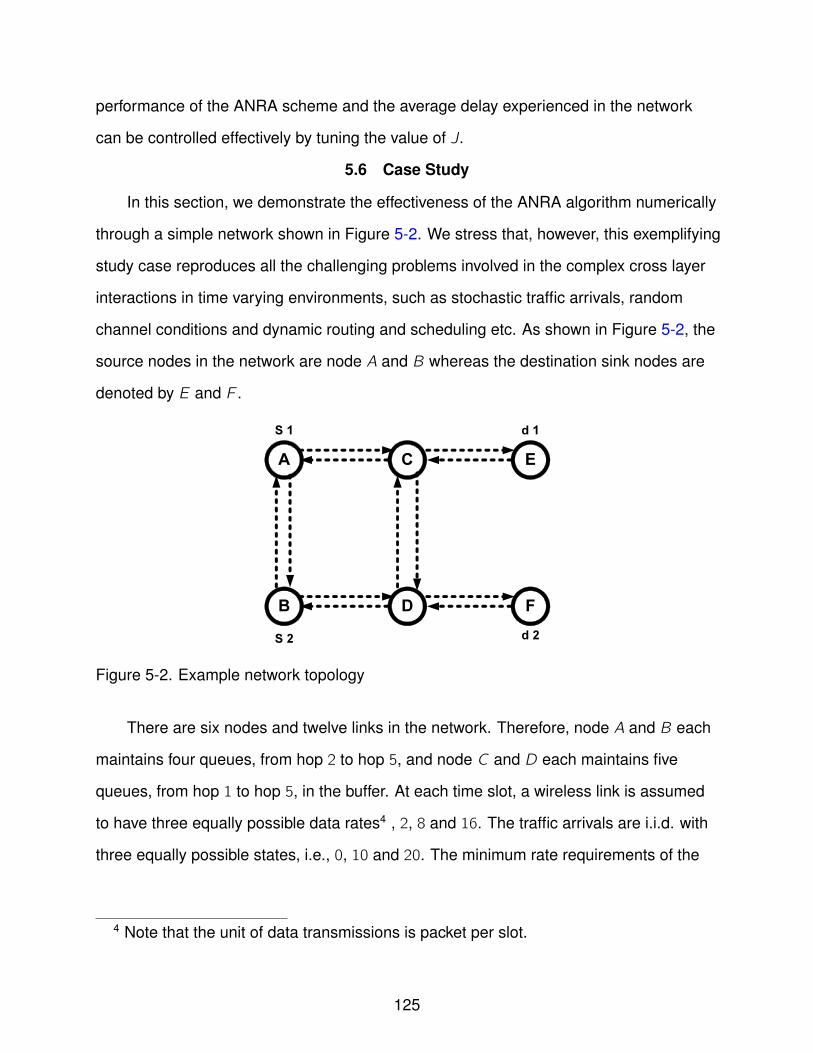
performance of the ANRA scheme and the average delay experienced in the network
can be controlled effectively by tuning the value of J.
5.6 Case Study
In this section, we demonstrate the effectiveness of the ANRA algorithm numerically
through a simple network shown in Figure 5-2. We stress that, however, this exemplifying
study case reproduces all the challenging problems involved in the complex cross layer
interactions in time varying environments, such as stochastic traffic arrivals, random
channel conditions and dynamic routing and scheduling etc. As shown in Figure 5-2, the
source nodes in the network are node A and B whereas the destination sink nodes are
denoted by E and F .
F
ECA
DB
d 1
d 2
S 1
S 2
Figure 5-2. Example network topology
There are six nodes and twelve links in the network. Therefore, node A and B each
maintains four queues, from hop 2 to hop 5, and node C and D each maintains five
queues, from hop 1 to hop 5, in the buffer. At each time slot, a wireless link is assumed
to have three equally possible data rates4 , 2, 8 and 16. The traffic arrivals are i.i.d. with
three equally possible states, i.e., 0, 10 and 20. The minimum rate requirements of the
4 Note that the unit of data transmissions is packet per slot.
125
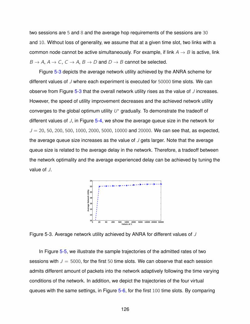
two sessions are 5 and 8 and the average hop requirements of the sessions are 30
and 10. Without loss of generality, we assume that at a given time slot, two links with a
common node cannot be active simultaneously. For example, if link A → B is active, link
B → A, A→ C , C → A, B → D and D → B cannot be selected.
Figure 5-3 depicts the average network utility achieved by the ANRA scheme for
different values of J where each experiment is executed for 50000 time slots. We can
observe from Figure 5-3 that the overall network utility rises as the value of J increases.
However, the speed of utility improvement decreases and the achieved network utility
converges to the global optimum utility U∗ gradually. To demonstrate the tradeoff of
different values of J, in Figure 5-4, we show the average queue size in the network for
J = 20, 50, 200, 500, 1000, 2000, 5000, 10000 and 20000. We can see that, as expected,
the average queue size increases as the value of J gets larger. Note that the average
queue size is related to the average delay in the network. Therefore, a tradeoff between
the network optimality and the average experienced delay can be achieved by tuning the
value of J.
0 20 50 200 500 1000 2000 5000 10000 20000 5000010
12
14
16
18
20
22
24
Values of J
Ave
rag
e N
etw
ork
Uti
lity
Figure 5-3. Average network utility achieved by ANRA for different values of J
In Figure 5-5, we illustrate the sample trajectories of the admitted rates of two
sessions with J = 5000, for the first 50 time slots. We can observe that each session
admits different amount of packets into the network adaptively following the time varying
conditions of the network. In addition, we depict the trajectories of the four virtual
queues with the same settings, in Figure 5-6, for the first 100 time slots. By comparing
126
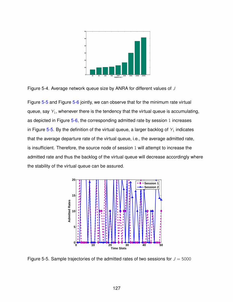
20 50 200 500 1000 2000 5000 10000 200000
100
200
300
400
500
600
Values of J
Figure 5-4. Average network queue size by ANRA for different values of J
Figure 5-5 and Figure 5-6 jointly, we can observe that for the minimum rate virtual
queue, say Y1, whenever there is the tendency that the virtual queue is accumulating,
as depicted in Figure 5-6, the corresponding admitted rate by session 1 increases
in Figure 5-5. By the definition of the virtual queue, a larger backlog of Y1 indicates
that the average departure rate of the virtual queue, i.e., the average admitted rate,
is insufficient. Therefore, the source node of session 1 will attempt to increase the
admitted rate and thus the backlog of the virtual queue will decrease accordingly where
the stability of the virtual queue can be assured.
0 10 20 30 40 500
5
10
15
20
Time Slots
Ad
mit
ted
Rat
es
Session 1Session 2
Figure 5-5. Sample trajectories of the admitted rates of two sessions for J = 5000
127
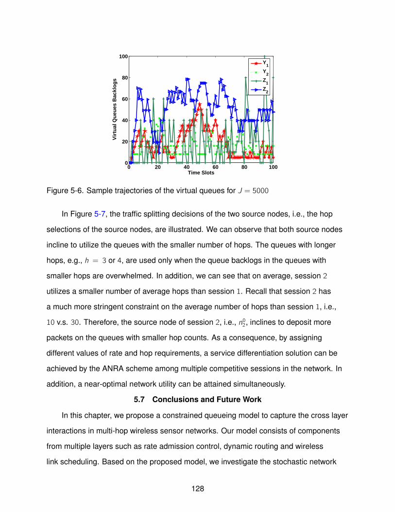
0 20 40 60 80 1000
20
40
60
80
100
Time Slots
Vir
tual
Qu
eues
Bac
klo
gs
Y1
Y2
Z1
Z2
Figure 5-6. Sample trajectories of the virtual queues for J = 5000
In Figure 5-7, the traffic splitting decisions of the two source nodes, i.e., the hop
selections of the source nodes, are illustrated. We can observe that both source nodes
incline to utilize the queues with the smaller number of hops. The queues with longer
hops, e.g., h = 3 or 4, are used only when the queue backlogs in the queues with
smaller hops are overwhelmed. In addition, we can see that on average, session 2
utilizes a smaller number of average hops than session 1. Recall that session 2 has
a much more stringent constraint on the average number of hops than session 1, i.e.,
10 v.s. 30. Therefore, the source node of session 2, i.e., n02, inclines to deposit more
packets on the queues with smaller hop counts. As a consequence, by assigning
different values of rate and hop requirements, a service differentiation solution can be
achieved by the ANRA scheme among multiple competitive sessions in the network. In
addition, a near-optimal network utility can be attained simultaneously.
5.7 Conclusions and Future Work
In this chapter, we propose a constrained queueing model to capture the cross layer
interactions in multi-hop wireless sensor networks. Our model consists of components
from multiple layers such as rate admission control, dynamic routing and wireless
link scheduling. Based on the proposed model, we investigate the stochastic network
128
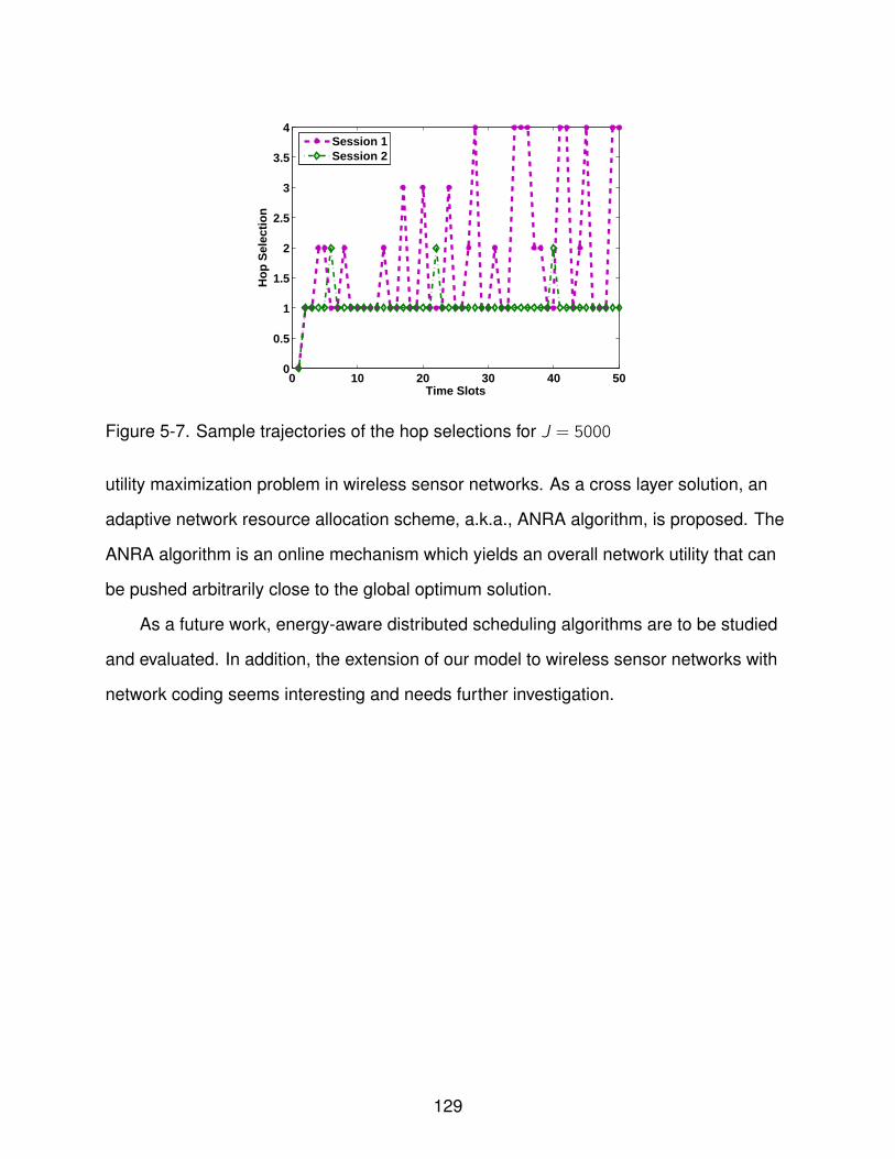
0 10 20 30 40 500
0.5
1
1.5
2
2.5
3
3.5
4
Time Slots
Ho
p S
elec
tio
n
Session 1Session 2
Figure 5-7. Sample trajectories of the hop selections for J = 5000
utility maximization problem in wireless sensor networks. As a cross layer solution, an
adaptive network resource allocation scheme, a.k.a., ANRA algorithm, is proposed. The
ANRA algorithm is an online mechanism which yields an overall network utility that can
be pushed arbitrarily close to the global optimum solution.
As a future work, energy-aware distributed scheduling algorithms are to be studied
and evaluated. In addition, the extension of our model to wireless sensor networks with
network coding seems interesting and needs further investigation.
129

CHAPTER 6THRESHOLD OPTIMIZATION FOR RATE ADAPTATION ALGORITHMS IN IEEE 802.11
WLANS
6.1 Introduction
IEEE 802.11 WLAN has become the dominating technology for indoor wireless
Internet access. While the original IEEE 802.11 DSSS only provides two physical data
rates (1 Mbps and 2 Mbps), the current IEEE standard provides several available data
rates based on different modulation and coding schemes. For example, IEEE 802.11b
supports 1 Mbps, 2 Mbps, 5.5 Mbps and 11 Mbps and IEEE 802.11g provides 12
physical data rates up to 54 Mbps. In order to maximize the network throughput, IEEE
802.11 devices, i.e., stations, need to adaptively change the data rate to combat with
the time-varying channel environments. For instance, when the channel is good, a high
data rate which usually requires higher SNR can be utilized. On the contrary, a low
data rate which is error-resilient might be favorable for a bad channel. The operation
of dynamically selecting data rates in IEEE 802.11 WLANs is called rate adaptation in
general.
The implementation of rate adaptation algorithms is not specified by the IEEE
802.11 standard. This intentional omission flourishes the studies on this active area
where a variety of rate adaptation algorithms have been proposed [92–108]. The
common challenge of rate adaptation algorithms is how to match the unknown channel
condition optimally such that the network throughput is maximized. According to the
methods of estimating channel conditions, rate adaptation algorithms can be divided into
two major categories. The first one is called closed-loop rate adaptation. Most schemes
in this approach enable the receiver to measure the channel quality and sends back
this information explicitly to the transmitter for rate adaptation. For example, the receiver
records the SNR or RSSI value of the received packet and sends this information back
to the transmitter via CTS or ACK packet. Consequently, the transmitter estimates the
channel condition based on the feedback signal and adjusts the data rate accordingly.
130

By utilizing additional feedback mechanisms, the close-loop rate adaptation algorithms
can achieve a better performance than the open-loop counterpart. However, in practice,
the close-loop rate adaptation algorithms are rarely used in commercial IEEE 802.11
devices. This is because that the extra feedback information needs to be conveyed
reliably and hence an inevitable modification on the current IEEE 802.11 standard is
needed. This non-compatibility hinders the close-loop rate adaptation algorithms from
practical implementations in current off-the-shelf IEEE 802.11 products.
The second category of rate adaptation algorithms, which is predominantly adopted
by the vendors, is labeled as open-loop algorithms. The widely utilized Auto Rate
Fallback algorithm, a.k.a., ARF, falls into this category. As many other open-loop rate
adaptation algorithms, ARF adjusts the date rate solely based on the IEEE 802.11
ACK packets. For example, in Enterasys RoamAbout IEEE 802.11 card [109], two
consecutive frame transmission failures, indicated by not receiving ACKs promptly,
induces a rate downshift, while ten consecutive successful frame transmissions triggers
a rate upshift [110]. Most commercialized IEEE products follow this up/down scheme
[95, 96]. In this chapter, we focus on the open-loop rate adaptation algorithms due to
the practical merits. More specifically, we consider a threshold-based rate adaptation
algorithm which works as follows. If there are θu consecutive successful transmissions,
the data rate is upgraded to the next level. On the other hand, if θd consecutive
transmissions failed, a rate downshift is triggered. Since ARF is merely a special
case of this threshold-based rate adaptation algorithm, our analysis can be applied to
ARF and its variants as well.
As a tradeoff with simplicity, there are several challenges existing for the threshold-based
rate adaptation algorithm. First, due to the trial-and-error based up/down mechanism, it
inherently lacks the capability of capturing short dynamics of the channel variations
[96]. To tackle this issue, Qiao et.al. propose a fast responsive rate adaptation
solution in [92]. By introducing a measure of “delay factor”, the responsiveness of the
131
threshold-based rate adaptation algorithm can be guaranteed. The second challenge
of the threshold-based rate adaptation algorithm is the indifference to collision-induced
failures and noise-induced failures. It is worth noting that in a multiuser WLAN, an ACK
timeout can be ascribed to either an MAC layer collision, or an erroneous channel.
However, the threshold-based rate adaptation algorithm is unable to distinguish them
effectively. Therefore, excessive collisions may introduce unnecessary rate degradations
which significantly deteriorate the system performance. Attributing the actual reason
of a transmission failure, or a packet loss, is named loss diagnosis [111] and has
attracted tremendous attention from the community. For example, Choi et.al. [112]
propose an algorithmic solution, which is specific to the threshold-based rate adaptation
algorithm, to mitigate the collision effect in multiuser IEEE 802.11 WLANs. Therefore,
the performance deterioration by the “indifference to collisions” can be compensated
effectively.
While the first two challenges of the threshold-based rate adaptation algorithm have
been tackled effectively, the third major obstacle, namely, the optimal selection of the
up/down thresholds, remains as an open problem. A systematic treatment on how to
select the values of θu and θd in the threshold-based rate adaptation algorithm is lacking
in the literature, although several heuristic solutions are proposed [93, 94].
The contribution of this work is twofold. First, we analytically investigate the
behavior of the threshold-based rate adaptation algorithm from a reverse engineering
perspective. In other words, we answer the essential yet unresolved question, i.e.,
“What is the threshold-based rate adaptation algorithm actually optimizing?”, by
unveiling the implicit objective function. As a result, several intuitive observations of
the threshold-based rate adaptation algorithm can be explained straightforwardly by
inspecting this objective function. Therefore, our reverse engineering model provides
an alternative means to understand the threshold-based rate adaptation algorithm. Our
work is a complement to the recent trend of reverse engineering studies on existing
132
heuristics-based networking protocols, such as TCP (transport layer) [4, 113, 114], BGP
(network layer) [115] and random access MAC protocol (data link layer) [116]. To the
best of our knowledge, this is the first work of studying threshold-based rate adaptation
algorithms from a reverse engineering perspective. Our results explicitly show that the
values of θu and θd play an important role in the objective function and thus the network
performance hinges largely on the selection of the up/down thresholds. In light of this,
we propose a threshold optimization algorithm which dynamically tunes the up/down
thresholds of the threshold-based rate adaptation algorithm and provably converges
to the stochastic optimum solution in arbitrary stationary random environments. We
show that the optimal selection of the thresholds significantly enhances the system’s
performance.
The rest of chapter is organized as follows. Section 6.2 briefly overviews the
state-of-the-art rate adaptation algorithms in the literature. The reverse engineering
model of the threshold-based rate adaptation algorithm is derived in Section 6.3.
In Section 6.4, the threshold optimization algorithm is proposed. The performance
evaluations are provided in Section 6.5 and Section 6.6 concludes this chapter.
6.2 Related Work
RBAR [103] proposes an SNR-based close-loop rate adaptation algorithm where
the rate decision relies on the feedback signal from the receiver. Specifically, the
receiver estimates the channel condition and determines a proper rate via the RTS/CTS
exchange. While consistently outperforms the open-loop rate adaptation algorithms
such as ARF, RBAR is incompatible with the current IEEE 802.11 standard by altering
the CTS frames [96]. In [105], a hybrid rate adaptation algorithm with SNR-based
measurements is proposed, where the measured SNR is utilized to bound the range
of feasible settings and thus shortens the response time to channel variations. [97] is
another example of the close-loop rate adaptation algorithms which attempts to improve
the throughput by predicting the channel coherence time, which is nevertheless difficult
133
in practice. Chen et.al. introduce a probabilistic-based rate adaptation for IEEE 802.11
WLANs. In [100], a rate-adaptive acknowledgement based rate adaptation algorithm is
introduced. The basic idea is that by varying the ACK transmission rate, the appropriate
rate information is conveyed to the transmitter. Wang and Helmy [108] propose a
traffic-aware rate adaptation algorithm which explicitly relates the background traffic to
the rate selection problem. However, aforementioned solutions either rely on altering the
frame structures, or do not conform to the de facto IEEE 802.11 standard in commercial
usage1 . CHARM [101] avoids the overhead of RTS/CTS by leveraging the channel
reciprocity. However, modifications on the IEEE 802.11 standardized frame structures,
e.g., beacons and probe signals, are still needed.
In light of the complexity and the incompatibility of the close-loop rate adaptation
algorithms, alternative open-loop rate adaptation algorithms are proposed. Although
usually providing inferior performance than the close-loop solutions, open-loop
algorithms soon become the predominant technique in commercial IEEE 802.11
devices due to the simplicity and the compatibility. The most popular open-loop rate
adaptation algorithm is the ARF protocol proposed by Ad and Leo [104] where a rate
upshift is triggered by ten consecutive successful transmission while two consecutive
failures induce a rate downshift. SampleRate [102] is another widely adopted open-loop
rate adaptation algorithm which performs arguably the best in static settings [96].
However, as pointed out by [96], SampleRate suffers from significant packet losses in
fast changing channels. ONOE [106] is a credit-based mechanism included in MadWiFi
drivers. The credit is determined by the number of successful transmissions, erroneous
transmissions and retransmissions jointly. However, it is pointed in [98] that ONOE is
less sensitive to individual packet failure and behaves over-conservatively.
1 For example, they largely rely on the RTS/CTS signaling mechanism which is hardlyused in practice.
134
As mentioned previously, one of the drawbacks of the simple open-loop rate
adaptation algorithms is the inability to discriminate the collision-induced losses and the
noise-induced losses. While several collision-aware rate adaptations are available in
the literature [95, 96, 99, 107], they base on the close-loop solutions which utilize either
RTS/CTS signaling or modifications on the standard. In [110], [112], Choi et.al. propose
a collision mitigation algorithm for open-loop ARF algorithm based on a Markovian
modeling. However, the channel conditions are assumed to be constant in their work. In
this work, on the contrary, we particularly focus on the threshold optimization to combat
with fast channel fluctuations rather than collisions. Therefore, in tandem with [110, 112],
our work provide a solution to jointly mitigate the channel fluctuations and the multiuser
collisions. For example, the up/down thresholds, i.e., θu and θd can be first calculated by
our threshold optimization algorithm in Section 6.4. Next, they are subjected to further
adjustments following [112] to mitigate the collision effects.
6.3 Reverse Engineering for the Threshold-Based Rate Adaptation Algorithm
We consider a station in a multi-rate IEEE 802.11 WLAN. There are N stations in
the WLAN where each station, say i , has a transmission probability of pi . Note that the
equivalence of the p-persistent model and the IEEE 802.11 binary exponential backoff
CSMA/CA model has been extensively studied in [116] and [117]. Throughout this work,
we assume that the transmission probability of each station is fixed. The interaction of
the data rate and the transmission probability remains as future research. Without loss
of generality, we assume that the stations have a same transmission probability of p.
In this work, we focus on the widely deployed open loop threshold-based rate
adaptation algorithm. Not surprisingly, the speed of channel variations has a great
impact on the performance of the rate adaptation algorithm. While the original intention
of the threshold-based rate adaptation algorithm is to maximize the average throughput,
a natural question arises that whether this is indeed the case. In this section, to better
understand the impact of θu and θd on the performance of the threshold-based rate
135
adaptation algorithm, we investigate the threshold-based rate adaptation algorithm via
a reverse engineering approach. We assume that the RTS/CTS signals are turned off.
In a time slot, say t, we denote the channel state2 as s(t) and denote the successful
transmission probability, given the current transmission rate r(t) and the channel
condition s(t), as
PS (s(t), r(t)) = p(1− p)N−1 (1− e(s(t), r(t))) (6–1)
where e denotes the frame error rate (FER) and is given by
e(s(t), r(t)) = 1− (1− Pe(s(t), r(t)))L (6–2)
and Pe(s(t), r(t)) is the bit error rate (BER) which is determined by the current data
rate, i.e., modulation scheme, and the current channel condition. L is the frame length of
the packet. Similarly, we define PF (s(t), r(t)) = 1 − PS(s(t), r(t)) as the transmission
failure probability at time t. It is worth noting that both PS and PF are functions of the
current data rate r(t) as well as the instantaneous channel condition s(t), which is
random. Particularly, we assume that the threshold-based rate adaptation algorithm
will increase the data rate by an amount of δ if there are θu consecutive successful
transmissions and decrease it by δ if there are θd consecutive failures. Denote u = θu − 1
and d = θd − 1 for notation succinctness. We define a binary indicator function ζ(t)
where ζ(t) = 1 means that the transmission at time slot t is successful and ζ(t) = 0
otherwise. Mathematically, the updating rule of the threshold-based rate adaptation
algorithm can be written as
2 Note that the number of feasible channel states can be potentially infinite.
136

r(t + 1) = (r(t) + δ)Γζ(t)=1Γζ(t−1)=1 · · ·Γζ(t−u)=1
+(r(t)− δ)Γζ(t)=0Γζ(t−1)=0 · · ·Γζ(t−d)=0
+r(t)Γo.w . (6–3)
where
Γx =
1, if event x is true
0, if event x is false.(6–4)
For example, Γζ(t)=1 = 1 if the transmission at time t is successful and Γζ(t)=1 = 0
otherwise. The symbol of o.w . denotes the event that neither θu consecutive successful
nor θd consecutive failed transmissions happened. For simplicity, we assume that the
maximum allowable data rate is sufficiently large and the minimum data rate is zero, i.e.,
not transmitting. Define
h(t) = [r(t), r(t − 1), · · · , r(1), e(s(t), r(t)), · · · , e(s(1), r(1))] (6–5)
as the history vector. In addition, we define
Z(t + 1) = E r(t + 1)|h(t) (6–6)
where E is the expectation operator.
Condition:
(C.1) The channel states between two consecutive successful transmissions or two
consecutive failed transmissions are independent random variables.
We emphasize that the restrictive condition (C.1) is not our general assumption in
this work. If (C.1) is satisfied, however, the derivation of the reverse engineering analysis
can be presented in a more concise form, as will be shown shortly.
137
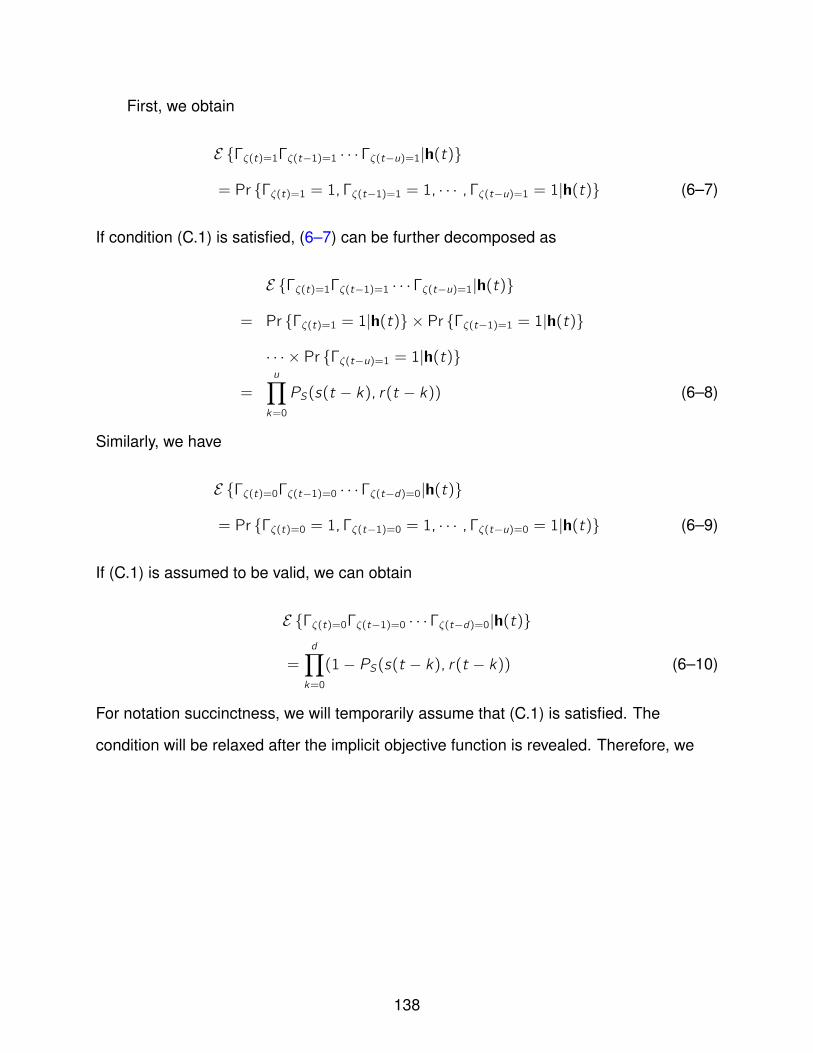
First, we obtain
E Γζ(t)=1Γζ(t−1)=1 · · ·Γζ(t−u)=1|h(t)
= Pr Γζ(t)=1 = 1, Γζ(t−1)=1 = 1, · · · , Γζ(t−u)=1 = 1|h(t) (6–7)
If condition (C.1) is satisfied, (6–7) can be further decomposed as
E Γζ(t)=1Γζ(t−1)=1 · · ·Γζ(t−u)=1|h(t)
= Pr Γζ(t)=1 = 1|h(t) × Pr Γζ(t−1)=1 = 1|h(t)
· · · × Pr Γζ(t−u)=1 = 1|h(t)
=
u∏k=0
PS(s(t − k), r(t − k)) (6–8)
Similarly, we have
E Γζ(t)=0Γζ(t−1)=0 · · ·Γζ(t−d)=0|h(t)
= Pr Γζ(t)=0 = 1, Γζ(t−1)=0 = 1, · · · , Γζ(t−u)=0 = 1|h(t) (6–9)
If (C.1) is assumed to be valid, we can obtain
E Γζ(t)=0Γζ(t−1)=0 · · ·Γζ(t−d)=0|h(t)
=
d∏k=0
(1− PS(s(t − k), r(t − k)) (6–10)
For notation succinctness, we will temporarily assume that (C.1) is satisfied. The
condition will be relaxed after the implicit objective function is revealed. Therefore, we
138
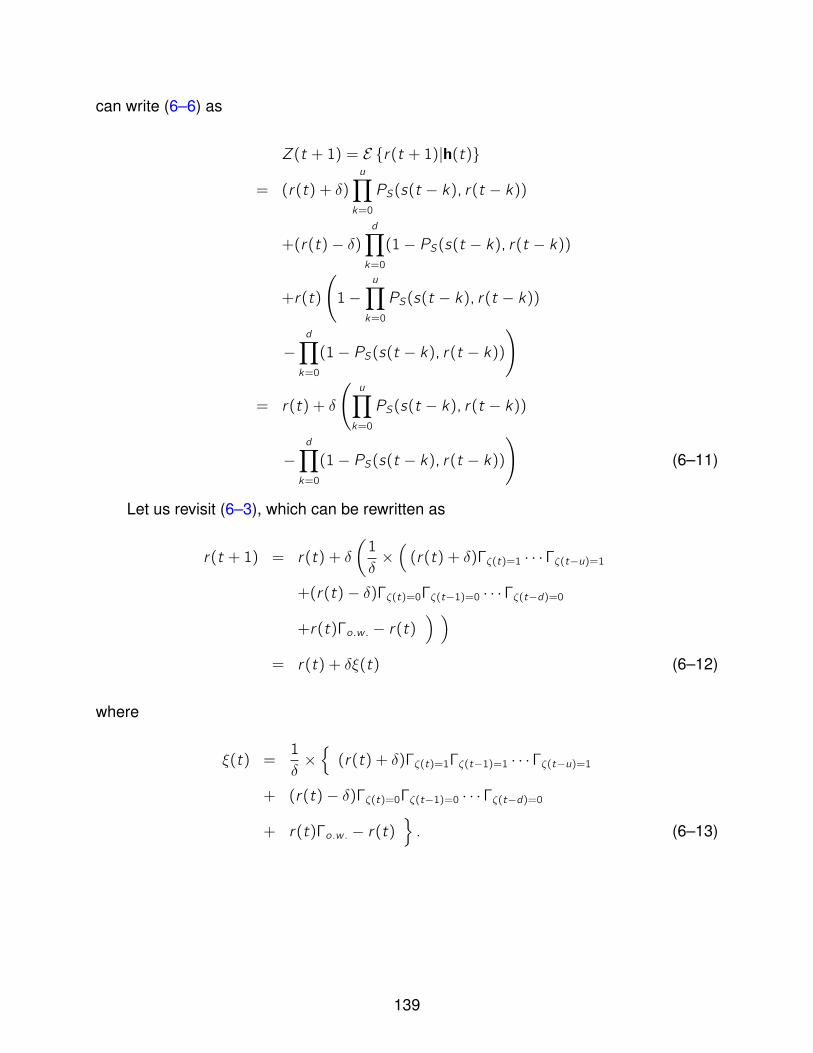
can write (6–6) as
Z(t + 1) = E r(t + 1)|h(t)
= (r(t) + δ)u∏k=0
PS(s(t − k), r(t − k))
+(r(t)− δ)d∏k=0
(1− PS(s(t − k), r(t − k))
+r(t)
(1−
u∏k=0
PS(s(t − k), r(t − k))
−d∏k=0
(1− PS(s(t − k), r(t − k))
)
= r(t) + δ
(u∏k=0
PS(s(t − k), r(t − k))
−d∏k=0
(1− PS(s(t − k), r(t − k))
)(6–11)
Let us revisit (6–3), which can be rewritten as
r(t + 1) = r(t) + δ
(1
δ×((r(t) + δ)Γζ(t)=1 · · ·Γζ(t−u)=1
+(r(t)− δ)Γζ(t)=0Γζ(t−1)=0 · · ·Γζ(t−d)=0
+r(t)Γo.w . − r(t)) )
= r(t) + δξ(t) (6–12)
where
ξ(t) =1
δ×(r(t) + δ)Γζ(t)=1Γζ(t−1)=1 · · ·Γζ(t−u)=1
+ (r(t)− δ)Γζ(t)=0Γζ(t−1)=0 · · ·Γζ(t−d)=0
+ r(t)Γo.w . − r(t). (6–13)
139

It should be noted that
Eξ(t)|h(t) =u∏k=0
PS(s(t − k), r(t − k))
−d∏k=0
(1− PS(s(t − k), r(t − k)). (6–14)
Therefore, we observe that (6–12) is a form of stochastic approximation with respect to
(6–11). Next, we present the reverse engineering theorem for the threshold-based rate
adaptation algorithm.
Theorem 6.1. The threshold-based rate adaptation algorithm of (6–3) is a stochastic
approximation which solves an implicit objective function U(t), with a constant stepsize
of δ, where U(t) is in the form of
U(t) = r(t)
u∏k=0
PS(s(t − k), r(t − k))
−d∏k=0
(1− PS(s(t − k), r(t − k))+K (6–15)
if condition (C.1) is satisfied and K is a constant with respect to rate r(t).
Proof. Theorem 1 follows directly from the previous analysis. Note that the threshold-based
rate adaptation algorithm can be written as
r(t + 1) = r(t) + δξ(t) (6–16)
where ξ(t) is the stochastic gradient and satisfies
Eξ(t)|h(t) = ∂U
∂r(t)|h(t) (6–17)
Hence Theorem 1 holds.
If condition (C.1) does not hold, we can replace
u∏k=0
PS(s(t − k), r(t − k))
140
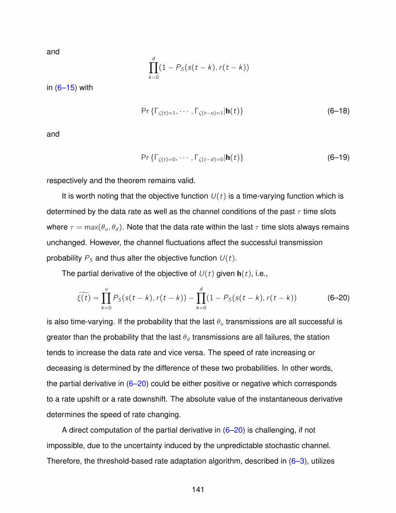
andd∏k=0
(1− PS(s(t − k), r(t − k))
in (6–15) with
Pr Γζ(t)=1, · · · , Γζ(t−u)=1|h(t) (6–18)
and
Pr Γζ(t)=0, · · · , Γζ(t−d)=0|h(t) (6–19)
respectively and the theorem remains valid.
It is worth noting that the objective function U(t) is a time-varying function which is
determined by the data rate as well as the channel conditions of the past τ time slots
where τ = max(θu, θd). Note that the data rate within the last τ time slots always remains
unchanged. However, the channel fluctuations affect the successful transmission
probability PS and thus alter the objective function U(t).
The partial derivative of the objective of U(t) given h(t), i.e.,
ξ(t) =u∏k=0
PS(s(t − k), r(t − k))−d∏k=0
(1− PS(s(t − k), r(t − k)) (6–20)
is also time-varying. If the probability that the last θu transmissions are all successful is
greater than the probability that the last θd transmissions are all failures, the station
tends to increase the data rate and vice versa. The speed of rate increasing or
deceasing is determined by the difference of these two probabilities. In other words,
the partial derivative in (6–20) could be either positive or negative which corresponds
to a rate upshift or a rate downshift. The absolute value of the instantaneous derivative
determines the speed of rate changing.
A direct computation of the partial derivative in (6–20) is challenging, if not
impossible, due to the uncertainty induced by the unpredictable stochastic channel.
Therefore, the threshold-based rate adaptation algorithm, described in (6–3), utilizes
141
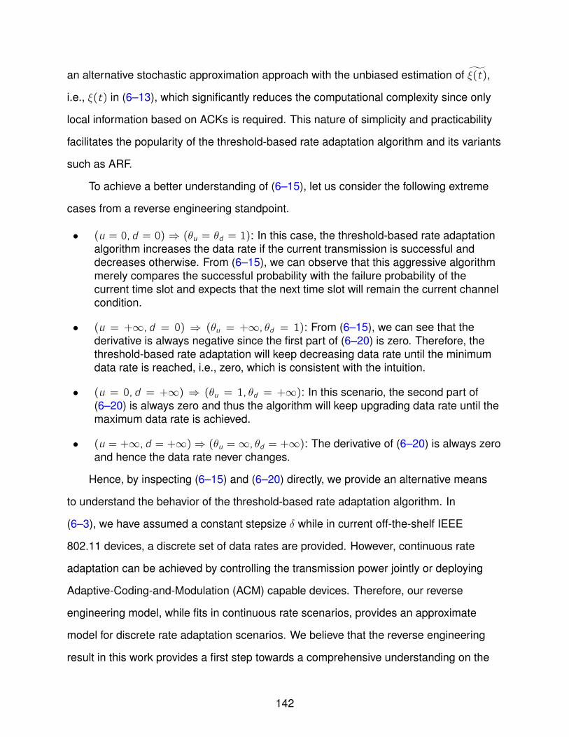
an alternative stochastic approximation approach with the unbiased estimation of ξ(t),
i.e., ξ(t) in (6–13), which significantly reduces the computational complexity since only
local information based on ACKs is required. This nature of simplicity and practicability
facilitates the popularity of the threshold-based rate adaptation algorithm and its variants
such as ARF.
To achieve a better understanding of (6–15), let us consider the following extreme
cases from a reverse engineering standpoint.
• (u = 0, d = 0) ⇒ (θu = θd = 1): In this case, the threshold-based rate adaptationalgorithm increases the data rate if the current transmission is successful anddecreases otherwise. From (6–15), we can observe that this aggressive algorithmmerely compares the successful probability with the failure probability of thecurrent time slot and expects that the next time slot will remain the current channelcondition.
• (u = +∞, d = 0) ⇒ (θu = +∞, θd = 1): From (6–15), we can see that thederivative is always negative since the first part of (6–20) is zero. Therefore, thethreshold-based rate adaptation will keep decreasing data rate until the minimumdata rate is reached, i.e., zero, which is consistent with the intuition.
• (u = 0, d = +∞) ⇒ (θu = 1, θd = +∞): In this scenario, the second part of(6–20) is always zero and thus the algorithm will keep upgrading data rate until themaximum data rate is achieved.
• (u = +∞, d = +∞)⇒ (θu =∞, θd = +∞): The derivative of (6–20) is always zeroand hence the data rate never changes.
Hence, by inspecting (6–15) and (6–20) directly, we provide an alternative means
to understand the behavior of the threshold-based rate adaptation algorithm. In
(6–3), we have assumed a constant stepsize δ while in current off-the-shelf IEEE
802.11 devices, a discrete set of data rates are provided. However, continuous rate
adaptation can be achieved by controlling the transmission power jointly or deploying
Adaptive-Coding-and-Modulation (ACM) capable devices. Therefore, our reverse
engineering model, while fits in continuous rate scenarios, provides an approximate
model for discrete rate adaptation scenarios. We believe that the reverse engineering
result in this work provides a first step towards a comprehensive understanding on the
142
good-yet-simple rate adaptation algorithm designs. In addition, based on the unveiled
implicit objective function of (6–15), the interactions of rate adaptations among multiple
IEEE 802.11 stations can be investigated in a game theoretical framework.
It is immediate to observe from (6–15) and (6–20) that the selection of θu and θd
has significant impact on the performance of the rate adaptation algorithm. Ideally, the
rate adaptation algorithm attempts to find the data rate which maximizes the expected
throughput in the next time slot, i.e.,
r ′ = argmaxr r × PS(s(t + 1), r). (6–21)
Define
V = r × PS(s(t + 1), r). (6–22)
Therefore, if we can estimate the value of ∂V∂r
and relate it by
ξ(t)→ ∂V
∂r, (6–23)
then the threshold-based rate adaptation algorithm is indeed optimizing the expected
throughput via the stochastic approximation approach. However, to achieve a derivative
estimation of a general non-Markovian system is non-trivial [118] [119]. Moreover, if the
channel appears totally random, e.g., non-stationary and fast fading, there exists no
effective optimization-based solution unless certain level of knowledge on the channel
randomness is available. Therefore, in the next section, we will consider a stationary
random channel environment. Nevertheless, the stochastic channel can be slow-varying
or fast-varying following arbitrary probabilistic distributions. We propose a threshold
optimization algorithm which provably converges to the stochastic optimum values of θu
and θd and the overall performance of the network is remarkably enhanced.
6.4 Threshold Optimization Algorithm
In this section, we model the stochastic channel as a stationary random process
denoted by s(t). It is worth noting that if the channel is quasi-static, i.e., s(t) is a
143
piecewise constant function, the probing-based rate adaptation algorithms, e.g.,
SampleRate [102], can achieve good performance. It is interesting to observe that
even in a quasi-static environment, for different channel conditions, the optimal values of
θu and θd may be different. One feasible way to find the optimum values of θu and θd with
different channel conditions, in a quasi-static environment, is the sample-path based
policy iteration approach introduced in [120] and [121], based on the Markovian model of
the threshold-based rate adaptation algorithm proposed in [110].
However, it is arguable that the channel environment is stochastic and time-varying
in nature. Therefore, it is not unusual that the channel condition has already changed
before the optimization algorithm has reached a steady state solution. The algorithm
will be thereby consistently chasing after a moving object and thus the thresholds are
always chosen suboptimally. This is more severe in a fast fading stochastic environment.
In light of this, we alternatively pursue the stochastic optimum values of the thresholds
in a time-varying and potentially fast changing channel environment. That is to say,
we attempt to find the set of values for θu and θd which maximize the expected system
performance with respect to the random channel. Before elaborating further, we briefly
outline the learning automata techniques based on which our threshold optimization
algorithm is proposed.
6.4.1 Learning Automata
Learning automata techniques are first introduced in the control community where
in many scenarios, the system is time-varying and stochastic in nature. Therefore,
stochastic learning approaches are desired to address the stochastic control problem in
random systems. The basic idea of learning automata techniques can be described as
follows. We consider a stochastic environment and a set of finite actions available for the
decision maker. Each selected action induces an output from the random environment.
However, due to the stochastic nature, the outputs for a given input may be different
at different time instances. Based on observations, a learning automata algorithm is
144
expected to find an action which is the stochastic optimum solution in the sense that the
expected system’s objective is maximized.
At each decision instance, the decision maker selects one of the actions according
to a probability vector. The selected action is fed to the stochastic environment as
the input and a random output is attained. The gist of learning automata techniques
lies in the provable convergence to the ϵ-optimal solution, as will be defined later, in
arbitrary stationary random environment. Thanks to the practicality and applicability,
learning automata techniques have been broadly studied in various aspects of the
communication and networking literature such as [122][123] [124] [125]. In this work,
we propose a learning automata based threshold optimization algorithm which finds the
stochastic optimum values of the up/down thresholds efficiently in any stationary yet
potentially fast-varying random channel environment. The detailed implementations are
introduced next.
6.4.2 Achieving the Stochastic Optimal Thresholds
We consider an IEEE 802.11 station as the decision maker which adjusts the values
of θu and θd . Without loss of generality, we assume that the maximum value of θu and
θd are mu and md , i.e., the feasible set of θu is Au = 1, · · · ,mu and that of θd is given
by Ad = 1, · · · ,md. The station maintains two probability vectors Pu and Pd for Au
and Ad , respectively. The k-th element in Pu, i.e., Pku , denotes the probability that θu is
set to k . Pkd is defined analogously. Simply put, at each decision instance, the threshold
optimization algorithm randomly determines the values of θu and θd according to Pu and
Pd . Next, the probability vectors, i.e., Pu and Pd , are updated and the iteration continues
until convergence, i.e., Pm∗u = 1 and Pn∗d = 1 where m∗ and n∗ denote the stochastic
optimal values of θu and θd , respectively.
Define a time series denoted by t = [t0, t1, · · · ] where t0 denotes the starting time
and other elements represent the exact time instances when the data rate is changed.
145
Denote
T (j) = [tj−1, tj ], j = 1, 2, · · ·
as the j-th time period, or time duration. It is worth noting that within a particular time
period, say j , the value of the data rate, the values of thresholds, i.e., θu and θd , are
all fixed numbers. We denote these period-dependent parameters as3 r(j), θu(j) and
θd(j). With this observation, we utilize the time series t as the time series of decision
instances. More specifically, for example, at time tj , a rate change is triggered either by
θu(j) consecutive successful transmissions or θd(j) consecutive failed transmissions.
In tandem with the data rate up/down shift, new values of the thresholds, i.e., θu(j + 1)
and θd(j + 1) are determined by the threshold optimization algorithm according to the
probability vectors Pu and Pd .
Besides Pu and Pd , we introduce additional vectors for Au and Ad , namely, the
counting vectors Cu, Cd , the surplus vectors Su, Sd , the estimation vectors Du, Dd and
the comparison vectors Zu, Zd . The definitions of parameters of the algorithm are
provided as follows.
Algorithm:
Parameters4 :
– Pu (Pd ): The probability vector for θu (θd ) over Au (Ad ).
– mu (md ): The maximum value of θu (θd ), or equivalently, the cardinality of Au (Ad ).
– Cu (Cd ): The counting vector of θu (θd ) where the k-th element, i.e., C ku (C kd ),denotes the times that k has been selected as the value of θu (θd ).
– Su (Sd ): The surplus vector of θu (θd ) where the k-th element, i.e., Sku (Skd ), denotesthe accumulated throughput with θu = k (θd = k).
3 Note that with a slight abuse of notation, we use j to denote the j-th time duration.
4 We present the analogous definitions in the parenthesis.
146

– Du (Dd ): The estimation vector of θu (θd ) where the k-th element, i.e., Dku (Dkd ), iscalculated by Dku =
SkuC ku
(Dkd =SkdC kd
).
– R: The resolution parameter which is a positive integer and is tunable by thestation.
– δu (δd ): The stepsize parameter of θu (θd ) and is given by δu = 1mu×R (δd = 1
md×R).
– φu (φd ): The perturbation vector of θu (θd ) where the k-th element, i.e., φku (φkd ), isa zero mean random variable which is uniformly distributed in [− ρ
Cku (Ckd ), + ρ
Cku (Ckd )]+1−1
where ρ is a system parameter and is controllable by the station. The notation of[a, b]xy represents [max(a, y),min(b, x)].
– Zu (Zd ): The comparison vector of θu (θd ) where the k-th element, i.e., Z ku (Z kd ), isgiven by Z ku = Dku + φku (Z kd = D
kd + φ
kd ).
– B: The predefined convergence threshold, e.g., 1, which is determined by thestation.
– J: A running parameter which records the updated maximum achieved throughputduring one time period.
At time t0:
Initialization:
- The station sets Pu = [p1, · · · , pi , · · · , pmu ] where pi = 1mu
for all 1 ≤ i ≤ mu.Similarly, Pd is given by [p1, · · · , pi , · · · , pmd ] where pi = 1
mdfor all 1 ≤ i ≤ md .
- Initializes Cu, Cd , Su, Sd , Du and Dd to zeros.
- Randomly selects the values of θu(1) and θd(1), say m, n, according to Pu(1) andPd(1).
- Transmits with θu = m and θd = n until T (1) ends, i.e., a data rate change istriggered.
- Records the average throughput within T (1) as J.
At time tj(j ≥ 1):
Do:
- Records the average throughput during Tj as O(j). If O(j) > J, sets J = O(j) andremains J unchanged otherwise.
147
- Updates the m-th element in the surplus vector Su and the n-th element in Sd byadding the measured normalized throughput of the last time period, as Smu =Smu +
O(j)J
and Snd = Snd +
O(j)J
.
- Updates the counting vectors by adding one to the m-th counter in Cu and the n-thcounter in Cd , as Cmu = Cmu + 1 and C nd = C
nd + 1.
- Updates the m-th element in Du and the n-th element in Dd by Dmu =SmuCmu
and
Dnd =SndCnd.
- For every element in Zu and Zd , updates Z ku = Dku + φku, k = 1, · · · ,mu andZ kd = D
kd + φ
kd , k = 1, · · · ,md .
- Finds the element in Zu with the highest5 value of Z ku , k = 1, · · · ,mu, say, the m-thelement in Au.
- Similarly, finds the element in Zd which has the highest Z kd , k = 1, · · · ,md , say, then-th element in Ad .
- Updates the probability vectors of Pu and Pd as
Pku = max(Pku − δu, 0
)if k = m, k = 1, · · · ,mu
Pku = 1−∑k =m
Pku if k = m (6–24)
and
Pkd = max(Pkd − δd , 0
)if k = n, k = 1, · · · ,md
Pkd = 1−∑k =n
Pkd if k = n (6–25)
where δu = 1mu×R and δd = 1
md×R.
- With the updated probability vectors Pu and Pd , new values of θu and θd , i.e.,θu(j + 1) and θd(j + 1), are selected.
– Starts the transmissions in T (j + 1) with θu(j + 1) and θd(j + 1).
Until:
- max(Pu) ≥ B and max(Pd) ≥ B where B is the predefined convergence threshold.
5 Note that a tie can be easily broken by a random selection.
148
End
The proposed threshold optimization algorithm is similar to the stochastic estimator
learning automata proposed in [126]. The key feature of this genre of learning automata
is the randomness deliberately introduced by φku and φkd . Note that although φku and φkd
are zero mean random variables, their variances are dependent on the values of C ku
and C kd , respectively. Specifically, the variances approach to zeros with the increase
of the number of times that the corresponding values of θu and θd are selected. As a
consequence, the threshold optimization algorithm inclines to more reliable stochastic
estimates and thus possesses a faster convergence behavior than other learning
algorithms [126]. The values that have been selected less frequently still have the
chance of being considered as optimal. However, the missing probability diminishes to
zero along iterations. In the algorithm, the resolution parameter R controls the stepsize
of probability adjustment in the algorithm. A smaller value of R produces a fine-grained
probability adjustment yet unavoidably prolongs the convergence time. The convergence
threshold B determines the stopping criteria of the algorithm. Therefore, a tradeoff
between optimality and convergence rate can be adjusted by tuning the value of B.
The steady state behavior of the proposed threshold optimization algorithm is
provided in the following theorem.
Theorem 6.2. The proposed threshold optimization algorithm is ϵ-optimal for any
stationary channel environment with arbitrary distribution. Mathematically, for any
arbitrarily small ϵ > 0 and γ > 0, there exists a t ′ satisfying
Pr|1− Pm∗
u | < ϵ > 1− γ ∀t > t ′ (6–26)
and
Pr|1− Pn∗d | < ϵ > 1− γ ∀t > t ′ (6–27)
where m∗ and n∗ are the stochastic optimal values of θu and θd , respectively.
149

The proof of Theorem 6.2 follows similar lines as in [126] and is omitted for brevity.
For more discussions on the stochastic estimator algorithms, refer to [127] and [128]. In
the next section, we will demonstrate the efficacy of our proposed threshold optimization
algorithm via simulations.
6.5 Performance Evaluation
In this section, we evaluate the performance of the proposed threshold optimization
algorithm with simulations. For comparisons, we first implement the heuristics-based
threshold adjustment algorithms in [93] and [94]. In [93], the downshift threshold θd is
fixed to 1 and the default value of θu is 10. After θu successful transmissions, a data
upshift is triggered and if the first transmission after the rate upshift is successful, the
algorithm assumes that the link quality is improving rapidly [93]. Consequently, θu is
set to a small number, e.g., θu = 3, in order to capture the fast improving channel.
Otherwise, the algorithm assumes that the channel is changing slowly and thus a larger
value of θu is desired, e.g., θu = 10. We denote this threshold adaptation scheme
as DLA in our simulations. Another well-known threshold adjusting scheme, namely,
AARF, is proposed in [94]. Similarly, the rate downshift threshold is fixed to θd = 2
empirically. However, for θu, a binary exponential backoff scheme is applied. If the first
transmission after a rate upshift failed, the data rate is switched back to the previous rate
and the value of θu is doubled with a maximum value of 50. The value of θu is reset to 10
whenever a rate downshift is triggered.
To simulate the indoor office environment for IEEE 802.11 WLANs, we simulate
a Rayleigh fading channel environment. In other words, we assume a flat fading
environment. However, it could be either a fast fading or slow fading channel. The
Doppler spread (in Hz) corresponds to the channel fading speed where a large Doppler
spread value represents a fast fading channel and a small Doppler spread indicates a
slow-varying channel. It should be noted that the Doppler spread value describes the
time dispersive nature of the wireless channel [129], which is inversely proportional to
150
the channel coherence time. More specifically, we relate the channel coherence time Tc
and the Doppler spread value fm as [129]
Tc =0.423
fm. (6–28)
Therefore, a larger Doppler spread value indicates a small channel coherence time
which represents a fast fading scenario. We conduct the simulations under various
channel fading conditions via different Doppler spread values. We consider the
IEEE 802.11b PHY specification, i.e., the available data rates are 1 Mbps, 2 Mbps,
5.5 Mbps and 11 Mbps and the RTS/CTS signalling scheme is turned off. Since the
objective of our proposed threshold optimization algorithm is to combat with the channel
variation, the collision effect is omitted. Therefore, we consider a WLAN with one
station consistently transmitting packets to the AP. However, note that [112] provides a
complementary solution to mitigate the collision effect and thus our algorithms can work
collectively as a joint solution. We emphasize that this simplification does not induce
any loss of generality since although seemingly simple, it produces all the challenging
problems involved in rate adaptation algorithms in a time-varying stochastic channel
environment. The data traffic is generated using constant bit rate UDP traffic sources
and the frame size is set to 1024 octets. The power of the transmitter and the power of
thermal noise are set to 50 mW and 1 mW, respectively. The SNR-BER relation is given
by Table 6-1 which is derived from [130].
We vary the Doppler spread value to simulate the various channel fading speeds.
For each value of Doppler spread value, the simulation is executed for 1000 seconds and
the average throughput of the following algorithms6 , which are commonly based on the
6 The performance comparison of ARF and other open-loop rate adaptationalgorithms such as SampleRate and ONOE has been studied extensively in [96] and[98] for various channel conditions.
151
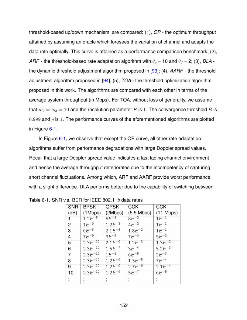
threshold-based up/down mechanism, are compared: (1), OP - the optimum throughput
attained by assuming an oracle which foresees the variation of channel and adapts the
data rate optimally. This curve is attained as a performance comparison benchmark; (2),
ARF - the threshold-based rate adaptation algorithm with θu = 10 and θd = 2; (3), DLA -
the dynamic threshold adjustment algorithm proposed in [93]; (4), AARF - the threshold
adjustment algorithm proposed in [94]; (5), TOA - the threshold optimization algorithm
proposed in this work. The algorithms are compared with each other in terms of the
average system throughput (in Mbps). For TOA, without loss of generality, we assume
that mu = md = 10 and the resolution parameter R is 1. The convergence threshold B is
0.999 and ρ is 1. The performance curves of the aforementioned algorithms are plotted
in Figure 6-1.
In Figure 6-1, we observe that except the OP curve, all other rate adaptation
algorithms suffer from performance degradations with large Doppler spread values.
Recall that a large Doppler spread value indicates a fast fading channel environment
and hence the average throughput deteriorates due to the incompetency of capturing
short channel fluctuations. Among which, ARF and AARF provide worst performance
with a slight difference. DLA performs better due to the capability of switching between
Table 6-1. SNR v.s. BER for IEEE 802.11b data ratesSNR BPSK QPSK CCK CCK(dB) (1Mbps) (2Mbps) (5.5 Mbps) (11 Mbps)1 1.2E−5 5E−3 8E−2 1E−1
2 1E−6 1.2E−3 4E−2 1E−1
3 6E−8 2.1E−4 1.8E−2 1E−1
4 7E−9 3E−5 7E−3 5E−2
5 2.3E−10 2.1E−6 1.2E−3 1.3E−2
6 2.3E−10 1.5E−7 3E−4 5.2E−3
7 2.3E−10 1E−8 6E−5 2E−3
8 2.3E−10 1.2E−9 1.3E−5 7E−4
9 2.3E−10 1.2E−9 2.7E−6 2.1E−4
10 2.3E−10 1.2E−9 5E−7 6E−5
......
......
...
152

2 4 6 8 10 12 141
2
3
4
5
6
7
8
Doppler Spread Value (Hz)
Ave
rag
e T
hro
ug
hp
ut
(Mb
ps)
OPARFDLAAARFTOA
Figure 6-1. Average throughput v.s. Doppler spread values
the large value and the small value of θu for different channel conditions. Our proposed
threshold optimization algorithm, as demonstrated in Figure 6-1, consistently outperforms
other open-loop rate adaptation algorithms and bridges the performance gap with the
OP curve. This superiority becomes remarkably significant in fast fading stochastic
channel environments, i.e., scenarios with large Doppler spread values. While other
algorithms are jeopardized by the unmature rate changes due to the uncertainty
caused by the random and fast-varying channel environment, our proposed threshold
optimization algorithm, based on the learning automata techniques, is able to find
the stochastic optimum values of θu and θd which maximize the expected system
performance. Therefore, our scheme is particularly suitable for fast changing yet
statistically stationary random channel environments where other open-loop rate
adaptation solutions usually provide unsatisfactory performance.
To illustrate the process of finding the stochastic optimum values of θu and θd , in
Figure 6-2, we provide the trajectories of θu and θd in a sample simulation run with a
fixed Doppler spread value of 10. It is observable that starting from the initial point, the
threshold optimization algorithm adapts the values of θu and θd on the fly along with the
rate changes. The algorithm soon finds the stochastic optimum values and θu and θd
converge to the optimum solutions effectively. The evolutions of the probability vectors,
153
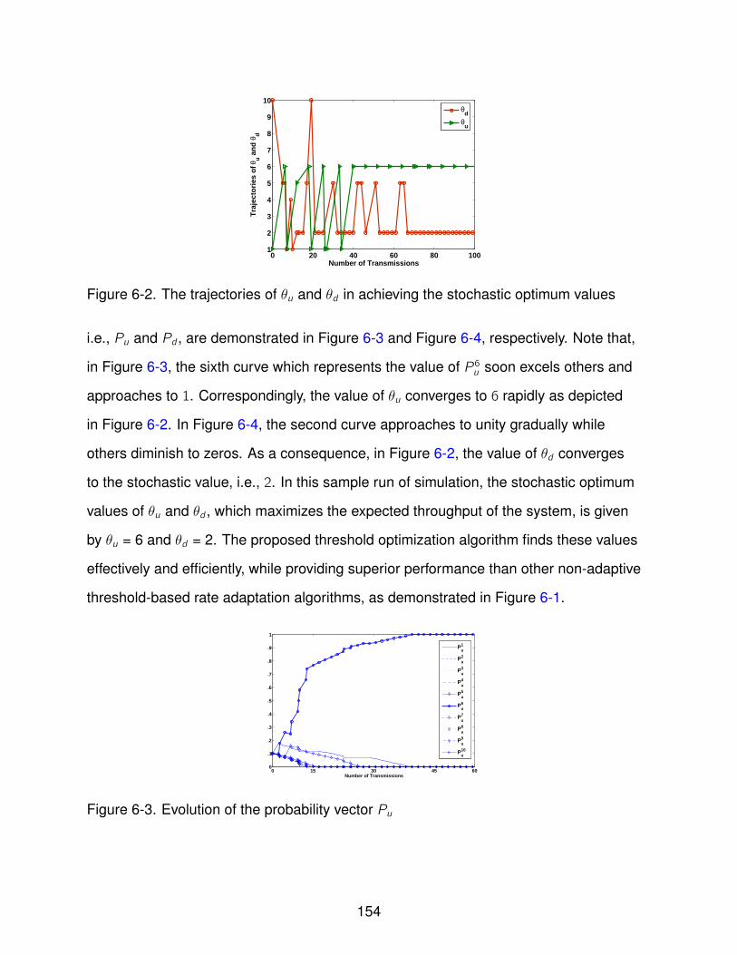
0 20 40 60 80 1001
2
3
4
5
6
7
8
9
10
Number of TransmissionsT
raje
cto
ries
of θ
u a
nd
θd
θd
θu
Figure 6-2. The trajectories of θu and θd in achieving the stochastic optimum values
i.e., Pu and Pd , are demonstrated in Figure 6-3 and Figure 6-4, respectively. Note that,
in Figure 6-3, the sixth curve which represents the value of P6u soon excels others and
approaches to 1. Correspondingly, the value of θu converges to 6 rapidly as depicted
in Figure 6-2. In Figure 6-4, the second curve approaches to unity gradually while
others diminish to zeros. As a consequence, in Figure 6-2, the value of θd converges
to the stochastic value, i.e., 2. In this sample run of simulation, the stochastic optimum
values of θu and θd , which maximizes the expected throughput of the system, is given
by θu = 6 and θd = 2. The proposed threshold optimization algorithm finds these values
effectively and efficiently, while providing superior performance than other non-adaptive
threshold-based rate adaptation algorithms, as demonstrated in Figure 6-1.
0 15 30 45 600
0.1
0.2
0.3
0.4
0.5
0.6
0.7
0.8
0.9
1
Number of Transmissions
Pu1
Pu2
Pu3
Pu4
Pu5
Pu6
Pu7
Pu8
Pu9
Pu10
Figure 6-3. Evolution of the probability vector Pu
154
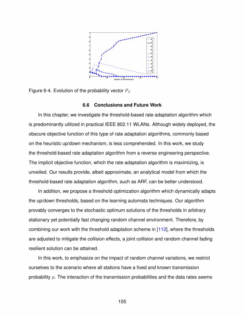
0 18 36 54 720
0.1
0.2
0.3
0.4
0.5
0.6
0.7
0.8
0.9
1
Number of Transmissions
Pd1
Pd2
Pd3
Pd4
Pd5
Pd6
Pd7
Pd8
Pd9
Pd10
Figure 6-4. Evolution of the probability vector Pd
6.6 Conclusions and Future Work
In this chapter, we investigate the threshold-based rate adaptation algorithm which
is predominantly utilized in practical IEEE 802.11 WLANs. Although widely deployed, the
obscure objective function of this type of rate adaptation algorithms, commonly based
on the heuristic up/down mechanism, is less comprehended. In this work, we study
the threshold-based rate adaptation algorithm from a reverse engineering perspective.
The implicit objective function, which the rate adaptation algorithm is maximizing, is
unveiled. Our results provide, albeit approximate, an analytical model from which the
threshold-based rate adaptation algorithm, such as ARF, can be better understood.
In addition, we propose a threshold optimization algorithm which dynamically adapts
the up/down thresholds, based on the learning automata techniques. Our algorithm
provably converges to the stochastic optimum solutions of the thresholds in arbitrary
stationary yet potentially fast changing random channel environment. Therefore, by
combining our work with the threshold adaptation scheme in [112], where the thresholds
are adjusted to mitigate the collision effects, a joint collision and random channel fading
resilient solution can be attained.
In this work, to emphasize on the impact of random channel variations, we restrict
ourselves to the scenario where all stations have a fixed and known transmission
probability p. The interaction of the transmission probabilities and the data rates seems
155

interesting and needs further investigation. Due to the competitive nature of channel
access, a stochastic game formulation may be utilized.
156
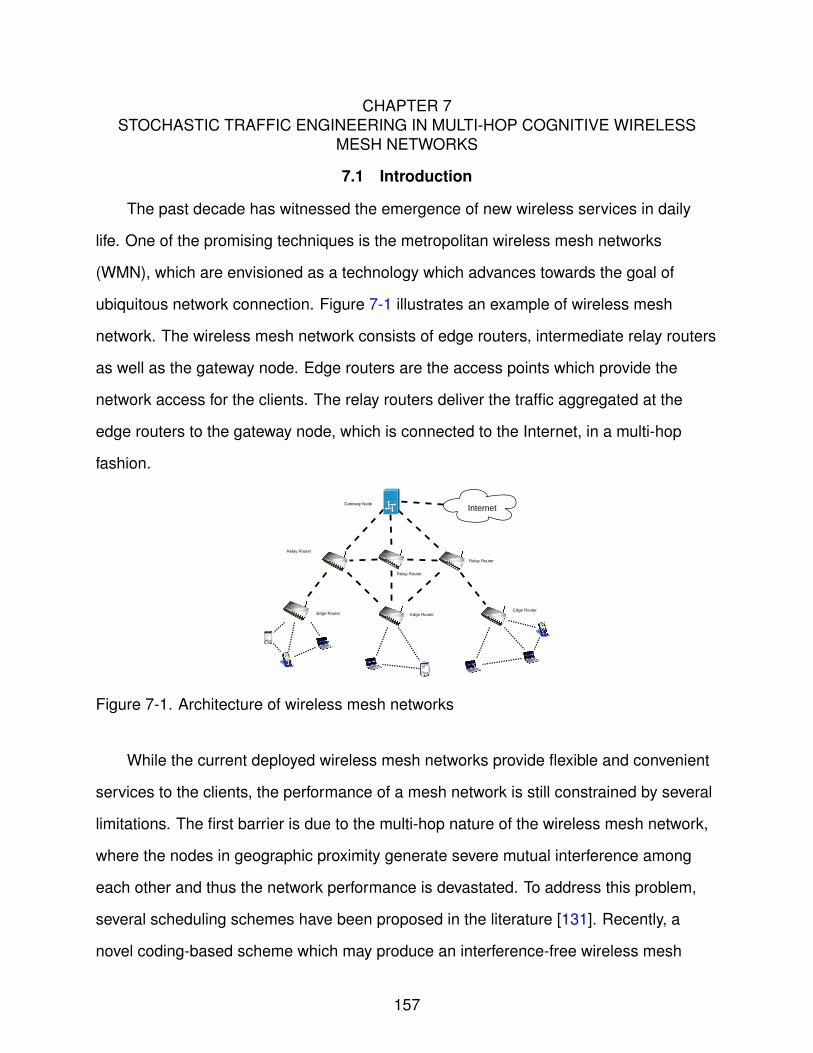
CHAPTER 7STOCHASTIC TRAFFIC ENGINEERING IN MULTI-HOP COGNITIVE WIRELESS
MESH NETWORKS
7.1 Introduction
The past decade has witnessed the emergence of new wireless services in daily
life. One of the promising techniques is the metropolitan wireless mesh networks
(WMN), which are envisioned as a technology which advances towards the goal of
ubiquitous network connection. Figure 7-1 illustrates an example of wireless mesh
network. The wireless mesh network consists of edge routers, intermediate relay routers
as well as the gateway node. Edge routers are the access points which provide the
network access for the clients. The relay routers deliver the traffic aggregated at the
edge routers to the gateway node, which is connected to the Internet, in a multi-hop
fashion.
InternetGateway Node
Relay Router
Relay Router
Relay Router
Edge Router Edge RouterEdge Router
Figure 7-1. Architecture of wireless mesh networks
While the current deployed wireless mesh networks provide flexible and convenient
services to the clients, the performance of a mesh network is still constrained by several
limitations. The first barrier is due to the multi-hop nature of the wireless mesh network,
where the nodes in geographic proximity generate severe mutual interference among
each other and thus the network performance is devastated. To address this problem,
several scheduling schemes have been proposed in the literature [131]. Recently, a
novel coding-based scheme which may produce an interference-free wireless mesh
157
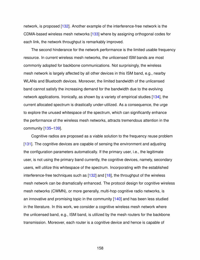
network, is proposed [132]. Another example of the interference-free network is the
CDMA-based wireless mesh networks [133] where by assigning orthogonal codes for
each link, the network throughput is remarkably improved.
The second hinderance for the network performance is the limited usable frequency
resource. In current wireless mesh networks, the unlicensed ISM bands are most
commonly adopted for backbone communications. Not surprisingly, the wireless
mesh network is largely affected by all other devices in this ISM band, e.g., nearby
WLANs and Bluetooth devices. Moreover, the limited bandwidth of the unlicensed
band cannot satisfy the increasing demand for the bandwidth due to the evolving
network applications. Ironically, as shown by a variety of empirical studies [134], the
current allocated spectrum is drastically under-utilized. As a consequence, the urge
to explore the unused whitespace of the spectrum, which can significantly enhance
the performance of the wireless mesh networks, attracts tremendous attention in the
community [135–139].
Cognitive radios are proposed as a viable solution to the frequency reuse problem
[131]. The cognitive devices are capable of sensing the environment and adjusting
the configuration parameters automatically. If the primary user, i.e., the legitimate
user, is not using the primary band currently, the cognitive devices, namely, secondary
users, will utilize this whitespace of the spectrum. Incorporating with the established
interference-free techniques such as [132] and [18], the throughput of the wireless
mesh network can be dramatically enhanced. The protocol design for cognitive wireless
mesh networks (CWMN), or more generally, multi-hop cognitive radio networks, is
an innovative and promising topic in the community [140] and has been less studied
in the literature. In this work, we consider a cognitive wireless mesh network where
the unlicensed band, e.g., ISM band, is utilized by the mesh routers for the backbone
transmission. Moreover, each router is a cognitive device and hence is capable of
158
sensing and exploiting the unused primary bands for transmissions whenever the
primary users are absent.
In this work, we investigate an important yet unexplored issue in the cognitive
wireless mesh networks, namely, the stochastic traffic engineering problem. More
specifically, we are particularly interested in how the traffic in the multi-hop cognitive
radio networks should be steered, under the influence of random behaviors of primary
users. It is worth noting that given a routing strategy, the corresponding network’s
performance, e.g., the average queueing delay encountered, is a random variable. The
reason is that the available bandwidth for a particular link depends on the appearance
of all the affecting primary users. If all the primary users are vacant, a link can utilize all
available frequency trunks collectively by utilizing advanced physical layer techniques,
e.g., OFDMA. However, if all the primary users are present, the only available frequency
space is the unlicensed ISM band and thus the traffic on this link will experience longer
delay than the previous case. In other words, the performance of a traffic engineering
solution hinges intensely on the unpredictable random behaviors of the primary users.
We emphasize that in multi-hop cognitive radio networks, this distinguishing feature of
randomness, induced by the random behaviors of primary users, must be taken into
account in protocol designs. Due to the location discrepancy, it is possible that some
node is affected by many primary users while others are not. As a consequence, if we
route the traffic via this particular node, the transmissions are more likely to be corrupted
by the returns of the primary users. Apparently, a favorable solution is more inclined to
steer the traffic from those “severely-affected area”, to the paths which are less affected
by the primary users. We will make this intuitive approach precise and rigorous in
this work. To our best knowledge, this work is the first work on the traffic engineering
problem in multi-hop cognitive radio networks, with a special focus on the impact of
random behaviors from the primary users.
159
The rest of this chapter is organized as follows. The related work is reviewed in
Section 7.2 and Section 7.3 provides the system model of our work. The stochastic
traffic engineering problem with convexity is investigated in Section 7.4. In Section 7.5,
we extend our framework to the non-convex stochastic traffic engineering problem.
Performance evaluation is provided in Section 7.6, followed by concluding remarks in
Section 7.7.
7.2 Related Work
Traditional traffic engineering (TE) algorithms are proposed as the solution to
the traffic management of the network in a cost-efficient manner. Different from the
traditional QoS routing, the traffic engineering solution not only guarantees a certain
QoS level for each flow, but also optimizes a global performance metric over the whole
network, by splitting the ingress traffic optimally among several available paths. The
multi-path routing is usually supported by the Multi-Protocol Label Switching (MPLS)
techniques where the explicit routing path for a packet is predetermined rather than
being computed in a hop-by-hop fashion. For a pair of source and destination nodes,
the set of available paths, a.k.a., label switched paths (LSP), are established and
managed by signalling protocols such as RSVP-TE [141] and CR-LDP [142] or manually
configuration. The traditional traffic engineering solution evolves to the stochastic
traffic engineering (STE) solution when uncertainty exists in the network, e.g., the
random returns of the primary users in our scenario. TE solutions require consistent
route changes which are unfavorable in that the network will be overwhelmed by the
oscillations induced by the unpredictable behaviors of the primary users. In light of this
stability concern, STE solution alternatively pursues an optimum multi-path routing
strategy such that the expected utility of the network is maximized. The stochastic traffic
engineering with uncertainties are discussed in the literature such as in [143] and [144].
However, the previous works usually assume a probability distribution of the uncertainty,
while in our scenario, the behaviors of the primary users are completely unpredictable
160
from the mesh network’s point of view. Distinguishing from the previous works, we
propose an algorithmic solution which requires no prior knowledge about the distribution
of the uncertainty, in a stochastic network utility maximization framework. It is worth
noting that our work differ from the traditional state-dependent traffic engineering
solution as well. For example, in [145], a state dependent traffic engineering solution is
proposed. However, the authors assume that the system state, i.e., the current value
of uncertainty, is fully observable. In our approach, we do not assume that the ingress
node has the perfect knowledge of the current appearance of the network. We will
discuss this issue in detail in Section 7.4.
Recently, cognitive wireless mesh networks (CWMN) have attracted great
attention in the literature. In [135], the channel assignment is discussed in a CWMN.
In [136], a cluster-based cognitive wireless mesh network framework is proposed.
The infrastructure-based cognitive network is discussed in [137] with a focus on the
cooperative mobility and the channel selection schemes. The spectrum sensing and
channel selection are jointly considered in a unified framework in [138]. In addition, the
IEEE 802.16h is in the process of incorporating the cognitive radios into the WiMAX
mesh networks [139]. However, none of the previous works considers the stochastic
traffic engineering problem. Therefore, a systematic study of the impacts of the random
returns from the primary users, on the network routing performance is lacking in the
existing literature. In [146], the joint congestion control and traffic engineering problem
is considered. He et.al. propose a distributed algorithm to balance the user’s utility and
the system’s objective. However, the authors assume the environment is fixed and does
not consider the randomness which is the distinguishing yet usually overlooked feature
in cognitive radio networks. [147] and [148] discuss the routing issue in cognitive radio
networks yet the impact of random returns of primary users is not investigated. Hou
et.al. [149] [150] [151] [152] formulate the joint routing, power and subband allocation
problem in cognitive radio networks as a mixed-integer programming. However, the
161
channels’ bandwidths are assumed to be fixed, i.e., the random behaviors of primary
users are still neglected. Our work is partially inspired by [153]. However, our work
differs from theirs in three crucial aspects. First, by targeting the stochastic traffic
engineering problem, our model differs from the joint power scheduling and rate control
work in [154]. Secondly, in [153, 154], the authors only consider a single-path scenario
while our work extends to a multi-path routing network where the network traffic can
be steered. Thirdly and most importantly, [153, 154] require that the current system
state is fully observable at the decision maker. To achieve this, the authors assume
a centralized mechanism which knows all the channel states of all the links over the
network. However, our work differs from [153, 154] significantly in that we do not require
that the current system’s state is known, which is of great practical interest since in
multi-hop cognitive wireless mesh networks, the decision makers, i.e., the edge routers
in our scenario, cannot be aware of the appearance of all primary users in the whole
network as a priori. Moreover, our schemes enjoy a decentralized implementation, in
contrast to centralized mechanisms in [153, 154], by utilizing the feedback signals and
local information only. In our previous work of [20], we proposed a routing optimization
scheme to combat with the randomness of instantaneous traffic in non-cognitive
wireless mesh networks. With respect to [20], this work differs in the following ways.
First, in the wireless mesh networks considered in [20], the capacity of each wireless
link is assumed to be fixed, i.e., time-invariant. However, in cognitive wireless mesh
networks, due to the unpredictable appearance of primary users, the bandwidth of each
wireless link is random. Secondly, in [20], the quality of service (QoS) requirement is
not considered. Nevertheless, in this chapter, we particularly address the QoS concern
of each user, e.g., the expected accumulated delay on the paths cannot exceed a
user-specific delay tolerance, as will be elaborated in Section 7.4. Thirdly and most
importantly, the analysis in [20] was based upon the assumption that the users all have
convex utility functions. In this work, we extend the techniques to address the scenarios
162
with non-convex utility functions. We will discuss the aforementioned issues further in
the following sections.
7.3 System Model
We consider a multi-hop wireless mesh network illustrated in Figure 7-1 where
an uplink traffic model is considered, i.e., all edge routers aggregate the traffic from
clients and deliver to the gateway node via the intermediate relay routers. To ensure
connectivity, we utilize the ISM 2.4G band as the underlying common channel for the
wireless mesh network. In addition, each link can utilize the opportunistic channels,
i.e., secondary bands to increase the link’s achievable data rate whenever the primary
user is vacant. We assume that there exists1 |M| primary users. Each primary user
possesses a licensed frequency channel and each mesh router is a cognitive node
which has the capability of sensing the current wireless environment. We model the
multi-hop cognitive wireless mesh network as a directional graph G where the vertices
are the nodes. We also denote link (i , j) as link e, e ∈ E where t(e) = i and r(e) = j
represent the transmitter and the receiver of link e.
We first consider a particular link denoted by (m, n). The instantaneous available
frequency bands, at time t, for a node i is denoted by Ii(t), which is determined by
the current presence of the primary users. Besides the underlying ISM band, the
communication between m and n can further utilize all secondary bands within
Im(t)∩In(t), if available. The current cognitive radio devices benefit largely from
the software-defined radio (SDR) techniques with advanced coding/modulation
capabilities. For example, by utilizing the multi-carrier modulation, e.g., OFDMA, a
cognitive radio device can utilize all the disjoint available frequency band simultaneously
[149, 150, 155–157]. At the transmitter, a software based radio combines waveforms
for different sub-bands and thus transmit signal at these sub-bands simultaneously.
1 The symbol of |X| represents the cardinality of the set X.
163
While at the receiver, a software based radio decomposes the combined waveforms
and thus receives signal at these sub-bands simultaneously [151, 152, 156, 157]. In
this work, we assume a spectrum sensing scheme available that each node can sense
the presence of the primary users in range, such as [131, 158], although the time of
random returns cannot be predicted. A link will utilize all the available vacant bands and
that the cognitive radios are full-duplex and can transmit at different bands concurrently
[151, 152, 156, 157]. We further assume that some scheduling mechanism is in place or
some physical layer mechanisms are utilized such that the nodes cannot interfere with
each other during the transmissions. For example, in a multi-channel multi-radio wireless
mesh network, the channels can be assigned properly that the transmissions do not
interfere with the neighboring nodes [132, 159]. Other examples are the OFDMA/CDMA
based wireless mesh networks [133, 160] where the interference among nodes can
be eliminated by assigning orthogonal subcarriers/codes. We emphasize that this
assumption is only for the sake of modeling simplicity and does not incur any loss of
generality, as will be clarified shortly.
It is worth noting that the available bandwidth of each link in the cognitive wireless
mesh network is a random variable. For example, at time instance t1, node m has three
secondary bands available, i.e., Im(t1) = I0, I1, I2, I3 and In(t1) = I0, I2, I3, I4, I5 due
to the location discrepancy, where band 0 is the underlying unlicensed ISM band and
1, 2, 3, 4, 5 are the licensed bands of primary users. The current bandwidth of link (m, n)
is represented byWm,n(t1) = BW0 + BW2 + BW3 where BWi is the bandwidth of
band i . At another time instance t2, the primary user 2 returns and the bandwidth of link
(m, n) becomesWm,n(t2) = BW0 + BW3. In other words, the bandwidth of links are
random variables which are determined by the unpredictable appearance of the primary
users. We model this randomness induced by the primary users as a stationary random
process with arbitrary distribution. The system is assumed to be time-slotted. In each
time slot n, the system state is assumed to be independent and is denoted by a state
164
vector s = δ1, · · · , δ|M|, s ∈ S, where δi = 1 denotes the absence of the i -th primary
user and 0 otherwise. We denote the stationary probability distribution of state s as
πs . For the ease of exposition, we assume that the primary users are static. However,
we emphasize that our model can be extended to mobile primary users scenarios
straightforwardly. For example, if a primary user is moving following a Markovian walk
model with well defined steady state distribution, the following analysis still applies.
Without loss of generality, we express the link capacity in the form of CDMA-based
networks, i.e., the capacity of a wireless link e ∈ E, given the system state s, is denoted
by c se , which is given by [4, 161] c se = W se1Tlog2(1 + Kγ
se), whereW s
e is the bandwidth of
link e in state s and γse is the current SINR value of link e. The constant T is the symbol
period and will be assumed to be one unit without loss of generality [4]. The constant
K = −Φ1log(Φ2BER)
where Φ1 and Φ2 are constants depending on the modulation scheme
and BER denotes the bit error rate. We will assume K = 1 in this work for simplicity
[161]. Note that our network model can be incorporated into other types of networks
such as MIMO, OFDM with TDMA or CSMA/CA based MAC protocols by modifying the
form of the capacity accordingly, which represents the achievable data rate in general.
For example, if we consider a scheduling-based MAC protocol where each link obtains
a time share of the channel access, the achievable data rate is given by c se = c se × ψe
where ψe is the fraction of time that the link is active following the scheduling scheme
and c se is the nominal Shannon capacity of the link.
There are |L| unicast sessions in the network, denoted by set L, where each
session l has a traffic demand dl . We associate each session with a unique user.
Therefore, we will use session l and user l interchangeably. For each session l ∈ L,
we denote the source node and destination node as S(l) and D(l), respectively. Recall
that we assume an uplink traffic model and thus all the source nodes are edge routers
and the destination node is the gateway. Furthermore, to improve the reliability and
165
dependability, we allow multi-path routing schemes. We denote the available2 set
of acyclic paths from S(l) to D(l) by Pl and the k-th path is represented by Pkl . We
introduce a parameter r kl as the flow allocated in the k-th path of session l . The overall
flow of user l , represented by xl , is given as
xl =
|Pl |∑k=1
r kl
dl0
(7–1)
where [x ]ba denotes maxminb, x, a. Define an |E|-by-|Pl | matrix Hl where the element
H le,k = 1 if link e is on the k-th path of Pl and 0 otherwise. Hence, H = H1, · · · ,H|L|
represents the network topology. Note that the traffic splitting and the source routing are
executed on the source node S(l).
For each link e ∈ E, there is an associated cost function, denoted by l se (fe, c se )
where fe is the accumulated flow on link e. We assume the function l se is an increasing,
differentiable and convex function of fe for a fixed c se . For example, if we assume
l se (fe, cse ) =
1cse−fe
when c se ≥ fe , the cost essentially represents the delay for a unit flow
on link e under the M/M/1 assumption. Note that in our scenario, even the accumulated
flow fe is fixed, the value of cost function is random due to the state-dependent variable
c se . From the network’s perspective, the stochastic traffic engineering solution will
distribute the aggregated flow among multiple paths optimally, in the sense that the
overall network utility is maximized. In next section, we will formulate the stochastic
traffic engineering problem in a stochastic network utility maximization framework [4] and
provide a distributed solution which requires no priori information about the underlying
probability distribution, i.e., πs , of the system states.
2 The available set of multiple paths can be obtained by signalling mechanisms suchas RSVP-TE[141] or pre-configured manually. In this work, we assume a predeterminedset of acyclic paths. The protocol design for acquiring such paths is beyond the scope ofthis work.
166

7.4 Stochastic Traffic Engineering with Convexity
7.4.1 Formulation
In the standard network utility maximization framework, each user has a utility
function Ul(xl), which reflects the degree of satisfaction of user l by transmitting at a rate
of xl , e.g., Ul(xl) = log(xl). In this section, we assume the utility functions to be concave
and differentiable. The non-convex utility functions are considered in Section 7.5. Note
that the fairness issue can be embodied in the utility functions [4]. For example, in the
seminal paper [113], the log-utility functions are adopted to achieve the proportional
fairness among different flows.
Define a feasible stochastic traffic engineering solution as r = [r1, · · · , r|L|] where
rl , [r 1l , · · · , r|Pl |l ]. We can formulate the stochastic traffic engineering problem as
P1 :
maxr≥0
∑l∈L
Ul(∑k∈Pl
r kl )
s.t.∑k∈Pl
r kl ≤ dl ∀l ∈ L (7–2)
∑s∈S
πs∑k∈Pl
r kl
∑e∈Pkl
l se (fe, cse )
≤ bl ∀l ∈ L (7–3)
fe ≤∑s∈S
πscse ∀e ∈ E (7–4)
fe =∑l∈L
∑k∈Pl
H le,krkl ∀e ∈ E (7–5)
c se =Wse
1
Tlog2(1 + Kγ
se) ∀e ∈ E (7–6)
where e ∈ Pkl represents the links along the k-th path of user l . The variable in P1 is
the vector of r. The first set of constraints reflect that the overall data rates of all paths
cannot exceed the traffic demand dl . The second set of constraints indicate that for
167
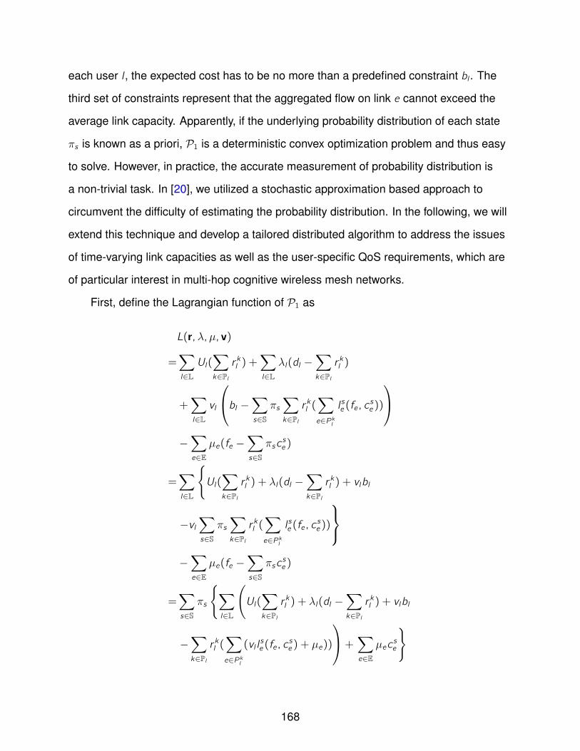
each user l , the expected cost has to be no more than a predefined constraint bl . The
third set of constraints represent that the aggregated flow on link e cannot exceed the
average link capacity. Apparently, if the underlying probability distribution of each state
πs is known as a priori, P1 is a deterministic convex optimization problem and thus easy
to solve. However, in practice, the accurate measurement of probability distribution is
a non-trivial task. In [20], we utilized a stochastic approximation based approach to
circumvent the difficulty of estimating the probability distribution. In the following, we will
extend this technique and develop a tailored distributed algorithm to address the issues
of time-varying link capacities as well as the user-specific QoS requirements, which are
of particular interest in multi-hop cognitive wireless mesh networks.
First, define the Lagrangian function of P1 as
L(r,λ,µ, v)
=∑l∈L
Ul(∑k∈Pl
r kl ) +∑l∈L
λl(dl −∑k∈Pl
r kl )
+∑l∈L
vl
bl −∑s∈S
πs∑k∈Pl
r kl (∑e∈Pkl
l se (fe, cse ))
−∑e∈E
µe(fe −∑s∈S
πscse )
=∑l∈L
Ul(∑k∈Pl
r kl ) + λl(dl −∑k∈Pl
r kl ) + vlbl
−vl∑s∈S
πs∑k∈Pl
r kl (∑e∈Pkl
l se (fe, cse ))
−∑e∈E
µe(fe −∑s∈S
πscse )
=∑s∈S
πs
∑l∈L
(Ul(∑k∈Pl
r kl ) + λl(dl −∑k∈Pl
r kl ) + vlbl
−∑k∈Pl
r kl (∑e∈Pkl
(vl lse (fe, c
se ) + µe))
+∑e∈E
µecse
168
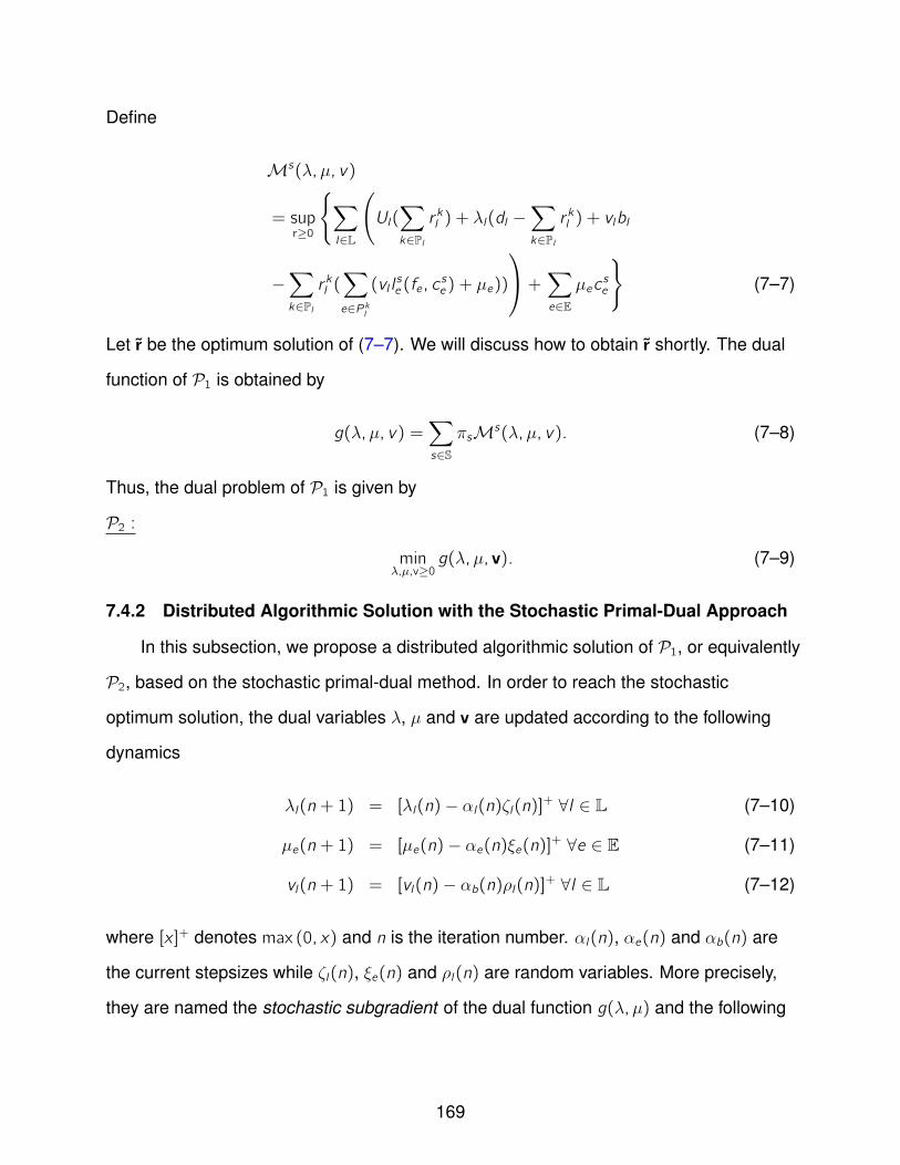
Define
Ms(λ,µ, v)
= supr≥0
∑l∈L
(Ul(∑k∈Pl
r kl ) + λl(dl −∑k∈Pl
r kl ) + vlbl
−∑k∈Pl
r kl (∑e∈Pkl
(vl lse (fe, c
se ) + µe))
+∑e∈E
µecse
(7–7)
Let r be the optimum solution of (7–7). We will discuss how to obtain r shortly. The dual
function of P1 is obtained by
g(λ,µ, v) =∑s∈S
πsMs(λ,µ, v). (7–8)
Thus, the dual problem of P1 is given by
P2 :
minλ,µ,v≥0
g(λ,µ, v). (7–9)
7.4.2 Distributed Algorithmic Solution with the Stochastic Primal-Dual Approach
In this subsection, we propose a distributed algorithmic solution of P1, or equivalently
P2, based on the stochastic primal-dual method. In order to reach the stochastic
optimum solution, the dual variables λ, µ and v are updated according to the following
dynamics
λl(n + 1) = [λl(n)− αl(n)ζl(n)]+ ∀l ∈ L (7–10)
µe(n + 1) = [µe(n)− αe(n)ξe(n)]+ ∀e ∈ E (7–11)
vl(n + 1) = [vl(n)− αb(n)ρl(n)]+ ∀l ∈ L (7–12)
where [x ]+ denotes max (0, x) and n is the iteration number. αl(n), αe(n) and αb(n) are
the current stepsizes while ζl(n), ξe(n) and ρl(n) are random variables. More precisely,
they are named the stochastic subgradient of the dual function g(λ,µ) and the following
169
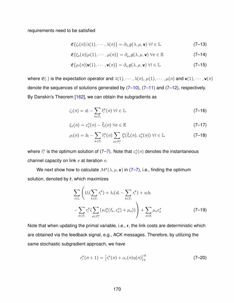
requirements need to be satisfied
Eζl(n)|λ(1), · · · ,λ(n) = ∂λlg(λ,µ, v) ∀l ∈ L (7–13)
Eξe(n)|µ(1), · · · ,µ(n) = ∂µeg(λ,µ, v) ∀e ∈ E (7–14)
Eρl(n)|v(1), · · · , v(n) = ∂vlg(λ,µ, v) ∀l ∈ L (7–15)
where E(.) is the expectation operator and λ(1), · · · ,λ(n), µ(1), · · · ,µ(n) and v(1), · · · , v(n)
denote the sequences of solutions generated by (7–10), (7–11) and (7–12), respectively.
By Danskin’s Theorem [162], we can obtain the subgradients as
ζl(n) = dl −∑k∈Pl
r kl (n) ∀l ∈ L (7–16)
ξe(n) = cse (n)− fe(n) ∀e ∈ E (7–17)
ρl(n) = bl −∑k∈Pl
r kl (n)∑e∈Pkl
l se (fe(n), cse (n)) ∀l ∈ L (7–18)
where r kl is the optimum solution of (7–7). Note that c se (n) denotes the instantaneous
channel capacity on link e at iteration n.
We next show how to calculate Ms(λ,µ, v) in (7–7), i.e., finding the optimum
solution, denoted by r, which maximizes
∑l∈L
(Ul(∑k∈Pl
r kl ) + λl(dl −∑k∈Pl
r kl ) + vlbl
−∑k∈Pl
r kl (∑e∈Pkl
(vl lse (fe, c
se ) + µe))
+∑e∈E
µecse (7–19)
Note that when updating the primal variable, i.e., r, the link costs are deterministic which
are obtained via the feedback signal, e.g., ACK messages. Therefore, by utilizing the
same stochastic subgradient approach, we have
r kl (n + 1) =[r kl (n) + αr(n)η(n)
]dl0
(7–20)
170
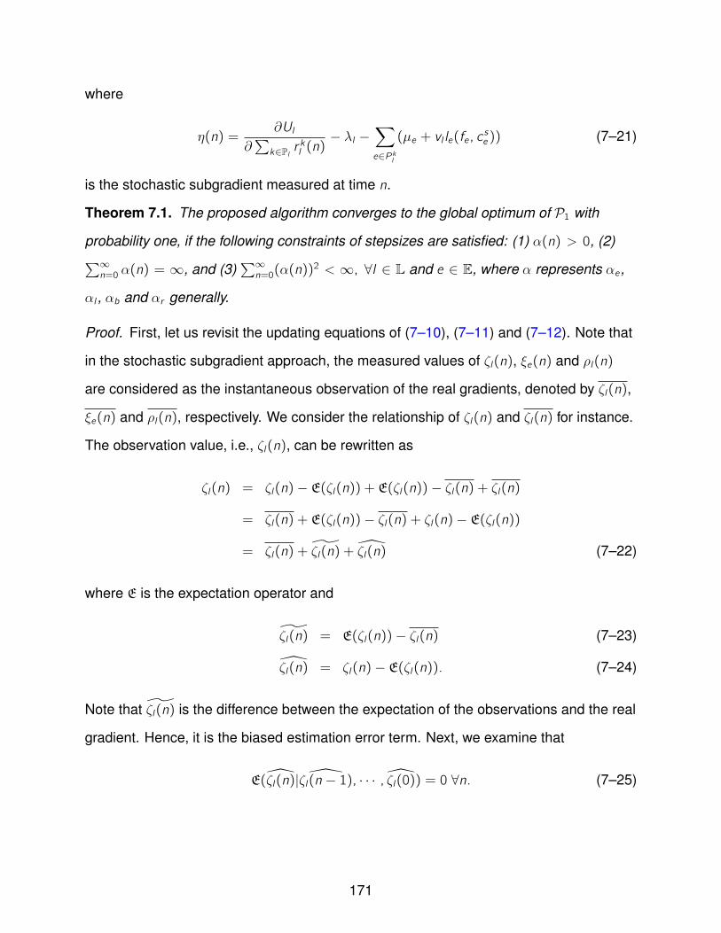
where
η(n) =∂Ul
∂∑k∈Pl r
kl (n)
− λl −∑e∈Pkl
(µe + vl le(fe, cse )) (7–21)
is the stochastic subgradient measured at time n.
Theorem 7.1. The proposed algorithm converges to the global optimum of P1 with
probability one, if the following constraints of stepsizes are satisfied: (1) α(n) > 0, (2)∑∞n=0 α(n) = ∞, and (3)
∑∞n=0(α(n))
2 < ∞, ∀l ∈ L and e ∈ E, where α represents αe ,
αl , αb and αr generally.
Proof. First, let us revisit the updating equations of (7–10), (7–11) and (7–12). Note that
in the stochastic subgradient approach, the measured values of ζl(n), ξe(n) and ρl(n)
are considered as the instantaneous observation of the real gradients, denoted by ζl(n),
ξe(n) and ρl(n), respectively. We consider the relationship of ζl(n) and ζl(n) for instance.
The observation value, i.e., ζl(n), can be rewritten as
ζl(n) = ζl(n)− E(ζl(n)) + E(ζl(n))− ζl(n) + ζl(n)
= ζl(n) + E(ζl(n))− ζl(n) + ζl(n)− E(ζl(n))
= ζl(n) + ζl(n) + ζl(n) (7–22)
where E is the expectation operator and
ζl(n) = E(ζl(n))− ζl(n) (7–23)
ζl(n) = ζl(n)− E(ζl(n)). (7–24)
Note that ζl(n) is the difference between the expectation of the observations and the real
gradient. Hence, it is the biased estimation error term. Next, we examine that
E(ζl(n)| ζl(n − 1), · · · , ζl(0)) = 0 ∀n. (7–25)
171

Therefore, the series of ζl(n) is a martingale difference sequence [163]. The relationship
of (7–22) indicates that the observation value is the real gradient disturbed by a biased
estimation error as well as a martingale difference noise. We next investigate the
convergence conditions of the stochastic primal-dual approach. For ζl(n), the following
requirement∞∑n=0
αe(n)|E(ζl(n))− ζl(n)| <∞ (7–26)
is satisfied due to the stationary assumption. Similarly,
E(ζl(n)2
) = E((ζl(n)− E(ζl(n)))
2)
(7–27)
is bounded as well. The similar analysis can be extended to ξe(n), ρl(n) and η(n) in
(7–11), (7–12) and (7–20) straightforwardly. Therefore, the standard conditions are
satisfied and the convergence result of Theorem 1 follows [8].
It is worth noting that the aforementioned distributed algorithm enjoys the merit of
distributed implementation from an engineering perspective. With the current values of
dual variables, each source node S(l) optimizes (7–19) according to (7–21) and (7–20).
The information needed is either locally attainable or acquirable by the feedback along
the paths. For example, the channel states of the intermediate nodes along paths can
be piggybacked by the end-to-end acknowledgement messages from the destination
node, i.e., the gateway node in our scenario. The source node updates the λl and vl
according to (7–10) and (7–12) where the needed information is calculated by (7–16)
and (7–18), respectively. For each link e, the current status of (7–17) is measured. Next,
the value of µe is updated following (7–11). The iteration continues until an equilibrium
point is reached. Note that our framework can incorporate the wireless lossy network
scenarios by replacing the flow rate with the effective flow rate in the leaky-pipe flow
model [164].
172

7.5 Stochastic Traffic Engineering without Convexity
Thus far, we have considered the scenarios where all the users have concave
utility functions. However, in practice, several network applications may possess a
non-concave utility function. For example, in a data streaming application, the user is
satisfied if the achieved data rate exceeds a threshold, where the utility function is a step
function and thus the convexity does not preserve. Therefore, the proposed stochastic
primal-dual approach in Section 7.4 cannot be applied here. It is worth noting that we
can still formulate the stochastic traffic engineering problem as in P1 except that the
optimization problem is a stochastic non-convex programming, which is NP-hard in
general, and computationally prohibitive to solve even in a centralized fashion [165].
In the following section, we will propose an algorithmic solution to the non-convex
stochastic traffic engineering problem, based on the learning automata techniques.
Moreover, we analytically show that the proposed algorithm will converge to the global
optimum solution asymptotically, in a decentralized fashion.
We first convert the compact strategy space of each user into a discretized set
denoted by R. More specifically, each user, say l , maintains a probability vector pl ,k for
each path k ∈ Pl . The segment of [0, rm] is quantized into Q sections where rm is the
maximum allowed transmission rate on any path. In other words, the continuous variable
r kl is transformed into a discrete random variable, r ql ,k , within a discretized set R with
Q + 1 elements. The data rate is randomly selected from R according to the probability
vector of pl ,k where the q-th element, pql ,k , q = 0, · · · ,Q, denotes the probability that the
l-th user transmits with a rate of r ql ,k = q × rm
Qon the k-th path of Pl . Associated with
each probability vector pl ,k , there is a weighting vector wl ,k with the same dimension of
1 × (Q + 1). The probability vector pl ,k is uniquely determined by the weighting vector
wl ,k by the softmax function [166],
pql ,k =ew
ql ,k∑Q
q=0 ewql ,k
∀l , k , q (7–28)
173
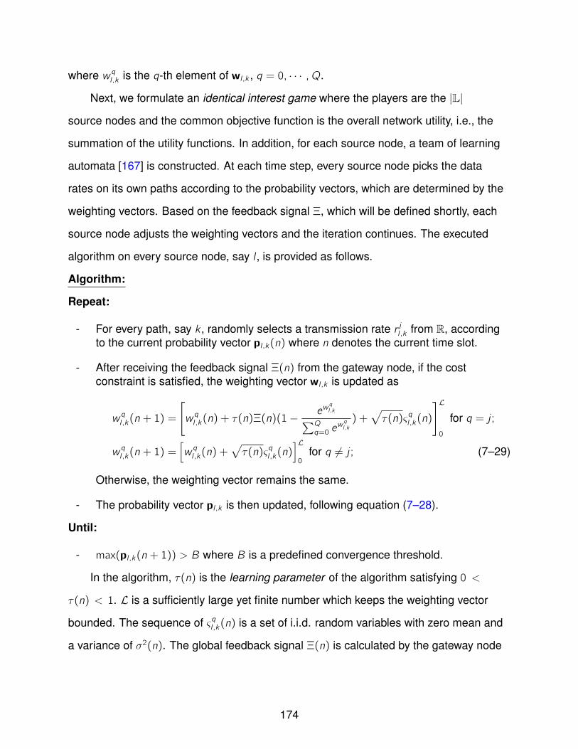
where w ql ,k is the q-th element of wl ,k , q = 0, · · · ,Q.
Next, we formulate an identical interest game where the players are the |L|
source nodes and the common objective function is the overall network utility, i.e., the
summation of the utility functions. In addition, for each source node, a team of learning
automata [167] is constructed. At each time step, every source node picks the data
rates on its own paths according to the probability vectors, which are determined by the
weighting vectors. Based on the feedback signal Ξ, which will be defined shortly, each
source node adjusts the weighting vectors and the iteration continues. The executed
algorithm on every source node, say l , is provided as follows.
Algorithm:
Repeat:
- For every path, say k , randomly selects a transmission rate r jl ,k from R, accordingto the current probability vector pl ,k(n) where n denotes the current time slot.
- After receiving the feedback signal Ξ(n) from the gateway node, if the costconstraint is satisfied, the weighting vector wl ,k is updated as
w ql ,k(n + 1) =
[w ql ,k(n) + τ(n)Ξ(n)(1−
ewql ,k∑Q
q=0 ewql ,k) +
√τ(n)ςql ,k(n)
]L0
for q = j ;
w ql ,k(n + 1) =[w ql ,k(n) +
√τ(n)ςql ,k(n)
]L0
for q = j ; (7–29)
Otherwise, the weighting vector remains the same.
- The probability vector pl ,k is then updated, following equation (7–28).
Until:
- max(pl ,k(n + 1)) > B where B is a predefined convergence threshold.
In the algorithm, τ(n) is the learning parameter of the algorithm satisfying 0 <
τ(n) < 1. L is a sufficiently large yet finite number which keeps the weighting vector
bounded. The sequence of ςql ,k(n) is a set of i.i.d. random variables with zero mean and
a variance of σ2(n). The global feedback signal Ξ(n) is calculated by the gateway node
174
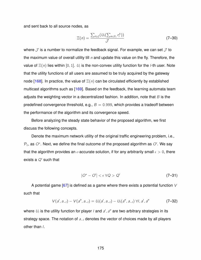
and sent back to all source nodes, as
Ξ(n) =
∑l∈L(Ul(
∑k∈Pl r
kl ))
J(7–30)
where J is a number to normalize the feedback signal. For example, we can set J to
the maximum value of overall utility till n and update this value on the fly. Therefore, the
value of Ξ(n) lies within [0, 1]. Ul is the non-convex utility function for the l-th user. Note
that the utility functions of all users are assumed to be truly acquired by the gateway
node [168]. In practice, the value of Ξ(n) can be circulated efficiently by established
multicast algorithms such as [169]. Based on the feedback, the learning automata team
adjusts the weighting vector in a decentralized fashion. In addition, note that B is the
predefined convergence threshold, e.g., B = 0.999, which provides a tradeoff between
the performance of the algorithm and its convergence speed.
Before analyzing the steady state behavior of the proposed algorithm, we first
discuss the following concepts.
Denote the maximum network utility of the original traffic engineering problem, i.e.,
P1, as O∗. Next, we define the final outcome of the proposed algorithm as O ′. We say
that the algorithm provides an ϵ-accurate solution, if for any arbitrarily small ϵ > 0, there
exists a Q ′ such that
|O∗ −O ′| < ϵ ∀Q > Q ′ (7–31)
A potential game [67] is defined as a game where there exists a potential function V
such that
V (a′, a−l)− V (a′′, a−l) = Ul(a′, a−l)− Ul(a′′, a−l) ∀l , a′, a′′ (7–32)
where Ul is the utility function for player l and a′, a′′ are two arbitrary strategies in its
strategy space. The notation of a−l denotes the vector of choices made by all players
other than l .
175
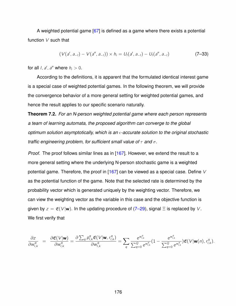
A weighted potential game [67] is defined as a game where there exists a potential
function V such that
(V (a′, a−l)− V (a′′, a−l))× hi = Ul(a′, a−l)− Ul(a′′, a−l) (7–33)
for all l , a′, a′′ where hi > 0.
According to the definitions, it is apparent that the formulated identical interest game
is a special case of weighted potential games. In the following theorem, we will provide
the convergence behavior of a more general setting for weighted potential games, and
hence the result applies to our specific scenario naturally.
Theorem 7.2. For an N-person weighted potential game where each person represents
a team of learning automata, the proposed algorithm can converge to the global
optimum solution asymptotically, which is an ϵ-accurate solution to the original stochastic
traffic engineering problem, for sufficient small value of τ and σ.
Proof. The proof follows similar lines as in [167]. However, we extend the result to a
more general setting where the underlying N-person stochastic game is a weighted
potential game. Therefore, the proof in [167] can be viewed as a special case. Define V
as the potential function of the game. Note that the selected rate is determined by the
probability vector which is generated uniquely by the weighting vector. Therefore, we
can view the weighting vector as the variable in this case and the objective function is
given by z = E(V |w). In the updating procedure of (7–29), signal Ξ is replaced by V .
We first verify that
∂z
∂w ql ,k=
∂E(V |w)∂w ql ,k
=∂∑q pql ,kE(V |w, r
ql ,k)
∂w ql ,k=∑q
ewql ,k∑Q
q=0 ewql ,k(1− ew
ql ,k∑Q
q=0 ewql ,k)E(V |w(n), r ql ,k).
176
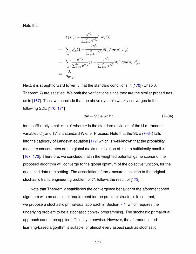
Note that
E(V (1− ewql ,k∑Q
q=0 ewql ,k)|w(n))
=∑q
pql ,k(1−ew
ql ,k∑Q
q=0 ewql ,k)E(V |w(n), r ql ,k)
=∑q
ewql ,k∑Q
q=0 ewql ,k(1− ew
ql ,k∑Q
q=0 ewql ,k)E(V |w(n), r ql ,k)
=∂z
∂w ql ,k.
Next, it is straightforward to verify that the standard conditions in [170] (Chap.6,
Theorem 7) are satisfied. We omit the verifications since they are the similar procedures
as in [167]. Thus, we conclude that the above dynamic weakly converges to the
following SDE [170, 171]
dw = ∇z + σdW (7–34)
for a sufficiently small τ → 0 where σ is the standard deviation of the i.i.d. random
variables ςql ,k and W is a standard Wiener Process. Note that the SDE (7–34) falls
into the category of Langevin equation [172] which is well-known that the probability
measure concentrates on the global maximum solution of z for a sufficiently small σ
[167, 172]. Therefore, we conclude that in the weighted potential game scenario, the
proposed algorithm will converge to the global optimum of the objective function, for the
quantized data rate setting. The association of the ϵ-accurate solution to the original
stochastic traffic engineering problem of P1 follows the result of [173].
Note that Theorem 2 establishes the convergence behavior of the aforementioned
algorithm with no additional requirement for the problem structure. In contrast,
we propose a stochastic primal-dual approach in Section 7.4, which requires the
underlying problem to be a stochastic convex programming. The stochastic primal-dual
approach cannot be applied efficiently otherwise. However, the aforementioned
learning-based algorithm is suitable for almost every aspect such as stochastic
177
non-convex programming and stochastic mixed-integer programming. The asymptotically
convergence result still holds. Therefore, in this work, the proposed algorithms
provide two different exemplifying methods for protocol designs under the stochastic
environment. However, it is worth noting that for the latter approach, the tradeoff for
general applicability is the convergence speed. In other words, in order to achieve an
accurate result, i.e., when ϵ is small, the convergence speed may be slow. The actual
convergence speed depends on the values of ϵ, Q, τ , σ as well as the inherent structure
of the problem and hence is difficult to quantify. Fortunately, in practical applications,
achieving a “good enough” result is sometimes satisfactory. This tradeoff can be
achieved by utilizing diminishing values of τ and σ, as demonstrated in the simulated
annealing literature [78] and [174]. To sum up, if the stochastic traffic engineering
problem possesses a nice property of convexity, the algorithm based on the stochastic
primal-dual approach in Section 7.4 is recommended due to its nice decomposed
structure and computationally efficient solution. However, if the problem is non-convex in
nature, the learning automata based algorithm can be utilized to achieve an approximate
solution. The tradeoff between the accuracy and convergence speed can be tuned by
adjusting the values of τ and σ.
7.6 Performance Evaluation
In this section, we present a simple yet illustrative example to demonstrate the
theoretical results. We consider a cognitive wireless mesh network3 depicted in Figure
7-2. There are three edge routers as the source nodes, denoted by A,B,C , which
transmit to the gateway node GW via the relay routers X ,Y and Z . Among all feasible
3 Figure 7-2 only shows the links on the available paths obtained by the signallingmechanisms or manually configurations. The actual physical topology of the networkcan be potentially larger.
178
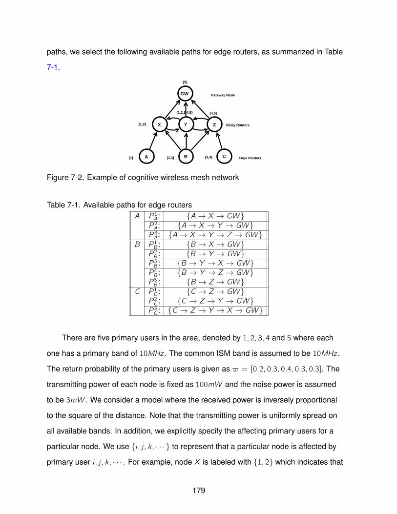
paths, we select the following available paths for edge routers, as summarized in Table
7-1.
GW
X Y Z
A B C Edge Routers
Relay Routers
Gateway Node
5
1,2
1 2,3 3,4
4,51,2,3,4,5
Figure 7-2. Example of cognitive wireless mesh network
Table 7-1. Available paths for edge routersA P1A: A→ X → GW P2A: A→ X → Y → GW P3A: A→ X → Y → Z → GW
B P1B : B → X → GW P2B : B → Y → GW P3B : B → Y → X → GW P4B : B → Y → Z → GW P5B : B → Z → GW
C P1C : C → Z → GW P2C : C → Z → Y → GW P3C : C → Z → Y → X → GW
There are five primary users in the area, denoted by 1, 2, 3, 4 and 5 where each
one has a primary band of 10MHz . The common ISM band is assumed to be 10MHz .
The return probability of the primary users is given as ϖ = [0.2, 0.3, 0.4, 0.3, 0.3]. The
transmitting power of each node is fixed as 100mW and the noise power is assumed
to be 3mW . We consider a model where the received power is inversely proportional
to the square of the distance. Note that the transmitting power is uniformly spread on
all available bands. In addition, we explicitly specify the affecting primary users for a
particular node. We use i , j , k , · · · to represent that a particular node is affected by
primary user i , j , k , · · · . For example, node X is labeled with 1, 2 which indicates that
179
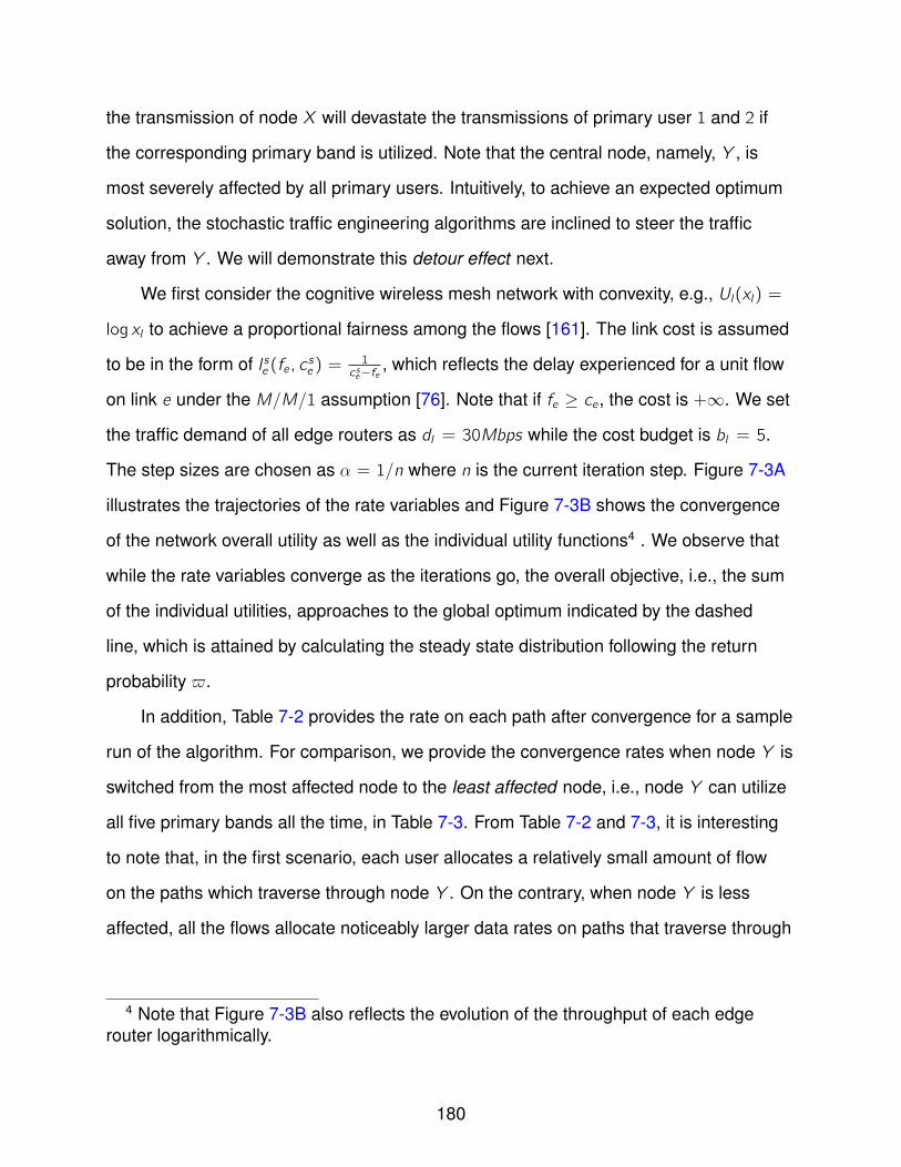
the transmission of node X will devastate the transmissions of primary user 1 and 2 if
the corresponding primary band is utilized. Note that the central node, namely, Y , is
most severely affected by all primary users. Intuitively, to achieve an expected optimum
solution, the stochastic traffic engineering algorithms are inclined to steer the traffic
away from Y . We will demonstrate this detour effect next.
We first consider the cognitive wireless mesh network with convexity, e.g., Ul(xl) =
log xl to achieve a proportional fairness among the flows [161]. The link cost is assumed
to be in the form of l se (fe, c se ) =1
cse−fe, which reflects the delay experienced for a unit flow
on link e under the M/M/1 assumption [76]. Note that if fe ≥ ce , the cost is +∞. We set
the traffic demand of all edge routers as dl = 30Mbps while the cost budget is bl = 5.
The step sizes are chosen as α = 1/n where n is the current iteration step. Figure 7-3A
illustrates the trajectories of the rate variables and Figure 7-3B shows the convergence
of the network overall utility as well as the individual utility functions4 . We observe that
while the rate variables converge as the iterations go, the overall objective, i.e., the sum
of the individual utilities, approaches to the global optimum indicated by the dashed
line, which is attained by calculating the steady state distribution following the return
probability ϖ.
In addition, Table 7-2 provides the rate on each path after convergence for a sample
run of the algorithm. For comparison, we provide the convergence rates when node Y is
switched from the most affected node to the least affected node, i.e., node Y can utilize
all five primary bands all the time, in Table 7-3. From Table 7-2 and 7-3, it is interesting
to note that, in the first scenario, each user allocates a relatively small amount of flow
on the paths which traverse through node Y . On the contrary, when node Y is less
affected, all the flows allocate noticeably larger data rates on paths that traverse through
4 Note that Figure 7-3B also reflects the evolution of the throughput of each edgerouter logarithmically.
180
0 10 20 30 40 50 60 70 80 90 1001
2
3
4
5
6
7
8
9
10
11
Iteration
Rat
e V
aria
bles
Convergence of Rate Variables
rA1
rA2
rA3
rB1
rB2
rB3
rB4
rB5
rC1
rC2
rC3
A Trajectories of Rate Variables
0 10 20 30 40 50 60 70 80 90 1000
1
2
3
4
5
6
7
8
9
10
Iteration
Util
ity F
unct
ions
Convergence of Overall Utility
Overall UtilityU
A
UB
UC
Global Optimum
B Trajectories of Utility Functions
Figure 7-3. Cognitive wireless mesh networks with convexity
Y despite the fact that node Y is the central node which is least favorable by traditional
traffic engineering solutions. Therefore, our proposed stochastic traffic engineering
algorithm is of particular interest for multi-hop cognitive wireless mesh networks due to
the capability of steering the traffic away from the severely affected areas automatically,
without a prior knowledge of the underlying probabilistic structure, in a distributed
fashion.
181

Table 7-2. Convergence rates when Y is affected by all five primary usersA P1A: 15.3035P2A: 3.2458P3A: 2.7362
B P1B : 7.3725P2B : 1.9584P3B : 2.1752P4B : 2.6458P5B : 5.3489
C P1C : 17.3051P2C : 2.3792P3C : 2.5675
Table 7-3. Convergence rates when Y is not affected by any of the primary usersA P1A: 9.6413P2A: 11.1335P3A: 9.1861
B P1B : 5.0101P2B : 6.2625P3B : 4.9711P4B : 4.9921P5B : 8.7878
C P1C : 15.3118P2C : 9.1042P3C : 5.6121
We next consider a cognitive wireless mesh network with non-convex utility
functions. Specifically, we consider the utility function as
Ul(xl) =
1, if xl ≥ 2Mbps
0, if xl < 2Mbps.(7–35)
while other settings are the same as in the previous scenario. Additionally, we utilize
diminishing values of τ and σ as τ = 1/n and σ = 1/n, where n is the iteration step5 .
Without loss of generality, we set L = 100 and the quantization level Q = 20. The
5 By utilizing diminishing parameters, a tradeoff between the performance and theconvergence speed can be achieved by tuning the decreasing speed [78].
182
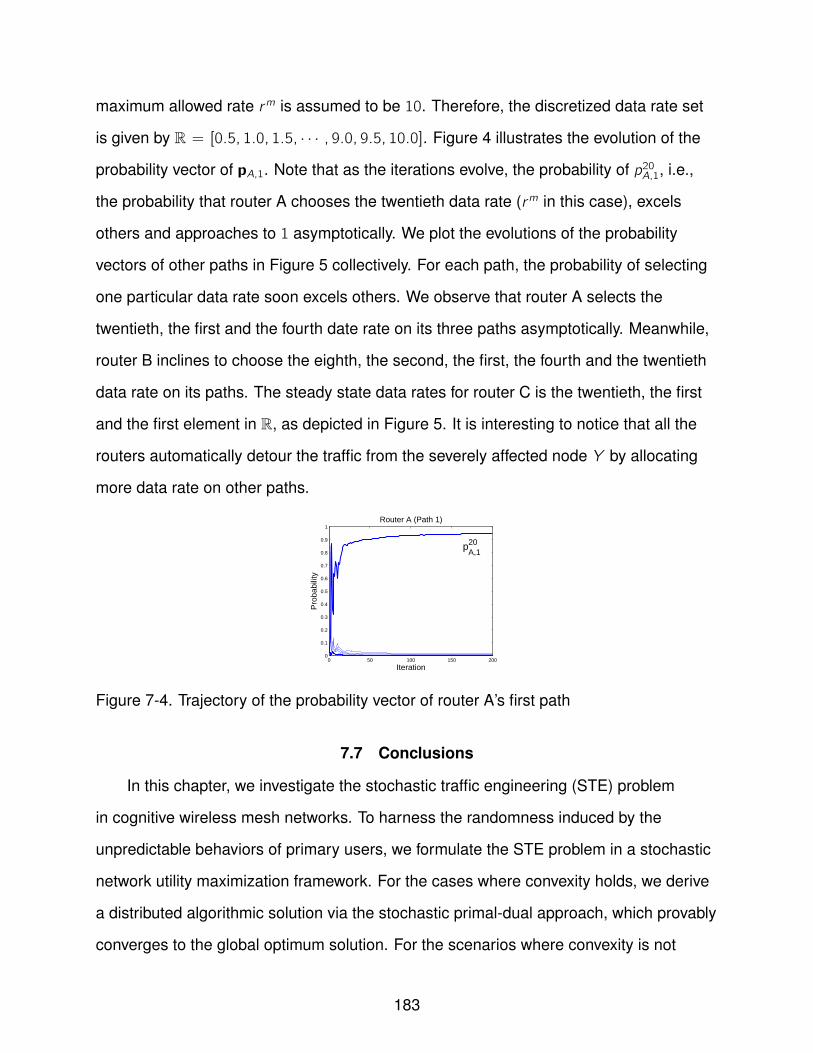
maximum allowed rate rm is assumed to be 10. Therefore, the discretized data rate set
is given by R = [0.5, 1.0, 1.5, · · · , 9.0, 9.5, 10.0]. Figure 4 illustrates the evolution of the
probability vector of pA,1. Note that as the iterations evolve, the probability of p20A,1, i.e.,
the probability that router A chooses the twentieth data rate (rm in this case), excels
others and approaches to 1 asymptotically. We plot the evolutions of the probability
vectors of other paths in Figure 5 collectively. For each path, the probability of selecting
one particular data rate soon excels others. We observe that router A selects the
twentieth, the first and the fourth date rate on its three paths asymptotically. Meanwhile,
router B inclines to choose the eighth, the second, the first, the fourth and the twentieth
data rate on its paths. The steady state data rates for router C is the twentieth, the first
and the first element in R, as depicted in Figure 5. It is interesting to notice that all the
routers automatically detour the traffic from the severely affected node Y by allocating
more data rate on other paths.
0 50 100 150 2000
0.1
0.2
0.3
0.4
0.5
0.6
0.7
0.8
0.9
1
Iteration
Pro
babi
lity
Router A (Path 1)
pA,120
Figure 7-4. Trajectory of the probability vector of router A’s first path
7.7 Conclusions
In this chapter, we investigate the stochastic traffic engineering (STE) problem
in cognitive wireless mesh networks. To harness the randomness induced by the
unpredictable behaviors of primary users, we formulate the STE problem in a stochastic
network utility maximization framework. For the cases where convexity holds, we derive
a distributed algorithmic solution via the stochastic primal-dual approach, which provably
converges to the global optimum solution. For the scenarios where convexity is not
183
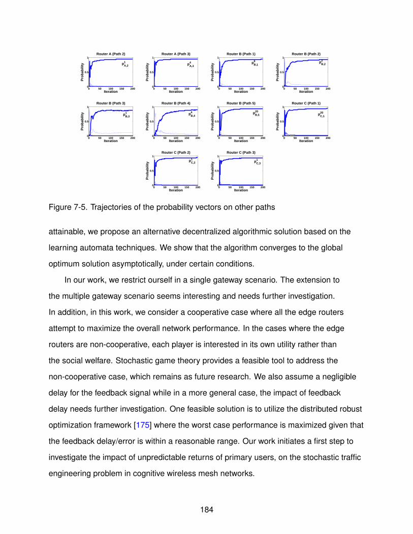
0 50 100 150 2000
0.5
1
Iteration
Pro
bab
ility
Router A (Path 2)
pA,21
0 50 100 150 2000
0.5
1
Iteration
Pro
bab
ility
Router A (Path 3)
pA,34
0 50 100 150 2000
0.5
1
Iteration
Pro
bab
ility
Router B (Path 1)
pB,18
0 50 100 150 2000
0.5
1
Iteration
Pro
bab
ility
Router B (Path 2)
pB,22
0 50 100 150 2000
0.5
1
Iteration
Pro
bab
ility
Router B (Path 3)
pB,31
0 50 100 150 2000
0.5
1
Iteration
Pro
bab
ility
Router B (Path 4)
pB,44
0 50 100 150 2000
0.5
1
Iteration
Pro
bab
ility
Router B (Path 5)
pB,520
0 50 100 150 2000
0.5
1
Iteration
Pro
bab
ility
Router C (Path 1)
pC,120
0 50 100 150 2000
0.5
1
Iteration
Pro
bab
ility
Router C (Path 2)
pC,21
0 50 100 150 2000
0.5
1
Iteration
Pro
bab
ility
Router C (Path 3)
pC,31
Figure 7-5. Trajectories of the probability vectors on other paths
attainable, we propose an alternative decentralized algorithmic solution based on the
learning automata techniques. We show that the algorithm converges to the global
optimum solution asymptotically, under certain conditions.
In our work, we restrict ourself in a single gateway scenario. The extension to
the multiple gateway scenario seems interesting and needs further investigation.
In addition, in this work, we consider a cooperative case where all the edge routers
attempt to maximize the overall network performance. In the cases where the edge
routers are non-cooperative, each player is interested in its own utility rather than
the social welfare. Stochastic game theory provides a feasible tool to address the
non-cooperative case, which remains as future research. We also assume a negligible
delay for the feedback signal while in a more general case, the impact of feedback
delay needs further investigation. One feasible solution is to utilize the distributed robust
optimization framework [175] where the worst case performance is maximized given that
the feedback delay/error is within a reasonable range. Our work initiates a first step to
investigate the impact of unpredictable returns of primary users, on the stochastic traffic
engineering problem in cognitive wireless mesh networks.
184
CHAPTER 8CONCLUSIONS
In this dissertation, we provide efficient and effective solutions to a number of
dynamic resource allocation and optimization problems in wireless networks with
time-varying channel conditions.
For wireless ad hoc networks, we first develop a dynamic pricing scheme which
can achieve a network-wide stability while maximizing the accumulated revenue with
a controllable tradeoff with the average delay. In addition, a service differentiation
solution can be achieved by prioritizing the flows according to their QoS requirements.
We also propose a minimum energy scheduling algorithm which minimizes the overall
energy consumption in the network without decreasing the throughput region. For
wireless mesh networks, we investigate the joint frequency and power allocation
problem among multiple access points in a game theoretical framework. The proposed
negotiation-based algorithm can achieve the optimal frequency and power allocation
with arbitrarily high probability. The price of anarchy in non-cooperative wireless mesh
networks is also studied. For wireless sensor networks, we propose a constrained
queueing model to capture the complex cross layer interactions among multiple sensor
nodes. We also study the stochastic network utility maximization problem and propose
a cross layer solution which solves the problems of admission control, load balancing,
dynamic scheduling and routing in a collective fashion. For wireless local area networks,
we study the thresholds-based rate adaptation algorithms from a reverse engineering
perspective, where the implicit objective function is revealed. We also investigate the
stochastic traffic engineering problem in multi-hop cognitive radio networks, where
distributed algorithms are developed to maximize the overall network utility.
185
REFERENCES
[1] G. R. Gupta and N. Shroff, “Delay analysis for multi-hop wireless networks,” IEEEINFOCOM, 2009.
[2] M. Andrews and L. Zhang, “Satisfying arbitrary delay requirements in multi-hopnetworks,” IEEE INFOCOM, 2008.
[3] M. Chiang, “Balancing transport and physical layer in wireless multihop networks:Jointly optimal congestion control and power control,” IEEE Journal on SelectedAreas in Communications, pp. 104–116, 2005.
[4] M. Chiang, S. H. Low, A. R. Calderbank, and J. C. Doyle, “Layering asoptimization decomposition: A mathematical theory of network architectures,”Proceedings of the IEEE, pp. 255–312, Mar. 2007.
[5] A. Eryilmaz and R. Srikant, “Fair resource allocation in wireless networks usingqueue-length-based scheduling and congestion control,” IEEE INFOCOM, 2005.
[6] F. Kelly, A. Maulloo, and D. Tan, “Rate control for communication networks:Shadow prices, proportional fairness and stability,” Journal of the OperationalResearch Society, pp. 237–252, 1998.
[7] S. H. Low and D. E. Lapsley, “Optimization flow control, i: Basic algorithm andconvergence,” IEEE/ACM Transactions on Networking, pp. 861–875, 1999.
[8] J. Zhang, D. Zheng, and M. Chiang, “The impact of stochastic noisy feedback ondistributed network utility maximization,” IEEE Transactions on Information Theory,2008.
[9] S. Boyd and L. Vandenberghe, Convex Optimization. Cambridge UniversityPress, 2003.
[10] R. Srikant, The Mathematics of Internet Congestion Control. Birkhauser Boston,2003.
[11] S. Shakkottai and R. Srikant, Network Optimization and Control. Foundationsand Trends in Networking, 2008.
[12] L. Tassiulas and A. Ephremides, “Stability properties of constrained queueingsystems and scheduling policies for maximum throughput in multihop radionetworks,” IEEE Transactions on Automatic Control, pp. 1936–1949, 1992.
[13] M. J. Neely, E. Modiano, and C. E. Rohrs, “Dynamic power allocation and routingfor time-varying wireless networks,” IEEE Journal on Selected Areas in Communi-cations, pp. 89–103, Jan. 2005.
186
[14] M. J. Neely, “Dynamic power allocation and routing for satellite and wirelessnetworks with time varying channels,” Ph.D. dissertation, Masssachusetts Instituteof Technology, LIDS, 2003.
[15] M. J. Neely, E. Modiano, and C.-P. Li, “Fairness and optimal stochastic control forheterogeneous networks,” IEEE/ACM Transactions on Networking, pp. 396–409,April 2008.
[16] M. J. Neely, “Energy optimal control for time varying wireless networks,” IEEETransactions on Information Theory, pp. 2915–2934, July 2006.
[17] L. Georgiadis, M. J. Neely, and L. Tassiulas, Resource Allocation and Cross-LayerControl in Wireless Networks. Foundations and Trends in Networking, 2006.
[18] Y. Xi and E. M. Yeh, “Distributed algorithms for spectrum allocation, power control,routing, and congestion control in wireless networks,” ACM MOBIHOC, 2007.
[19] ——, “Node-based optimal distributed power control, routing, and congestioncontrol in wireless networks,” IEEE Transactions on Information Theory, pp.4081–4106, 2008.
[20] Y. Song, C. Zhang, and Y. Fang, “Routing optimization in wireless mesh networksunder uncertain traffic demands,” ICST Fifth International Conference on Qualityof Service in Heterogeneous Wired/Wireless Networks (QShine), 2008.
[21] M. Andrews, K. Kumaran, K. Ramanan, A. Stolyar, P. Whiting, and R. Vijayakumar,“Providing quality of service over a shared wireless link,” IEEE CommunicationsMagazine, 2001.
[22] A. Stolyar, “Control of end-to-end delay tails in a multiclass network: Lwdfdiscipline optimality,” The Annals of Applied Probability, 2003.
[23] T. B. Reddy, I. Karthigeyan, B. S. Manoj, and C. S. R. Murthy, “Quality of serviceprovisioning in ad hoc wireless networks: A survey of issues and solutions,” AdHoc Networks, 2006.
[24] B. Zhang and H. T. Mouftah, “Qos routing for wireless ad hoc networks: Problems,algorithms, and protocols,” IEEE Communications Magazine, 2005.
[25] M. A. Zafer and E. Modiano, “A calculus approach to minimum energytransmission policies with quality of service guarantees,” IEEE INFOCOM, 2005.
[26] W. Chen, M. J. Neely, and U. Mitra, “Energy-efficient transmissions withindividual packet delay constraints,” IEEE Transactions on Information Theory,pp. 2090–2109, 2008.
[27] L. He and J. Walrand, “Pricing differentiated internet services,” IEEE INFOCOM,2005.
187
[28] T. Basar and R. Srikant, “Revenue-maximizaing pricing and capacity expansion ina many-users regime,” IEEE INFOCOM, 2002.
[29] R. K. Lam, D.-M. Chiu, and J. C. Lui, “On the access pricing and networkscaling issues of wireless mesh networks,” IEEE Transactions on Computers,pp. 1456–1469, 2007.
[30] Shakkottai and R. Srikant, “Economics of network pricing with multiple isps,”IEEE/ACM Transactions on Networking, 2006.
[31] N. J. Keon and G. Anandalingam, “Optimal pricing for multiple services intelecommunications networks offering quality-of-service guarantees,” IEEE/ACMTransactions on Networking, pp. 66–80, 2003.
[32] Z. Zhang, D. Dey, and Y. Tan, “Pricing communication services with delayguarantee,” INFORMS Journal on Computing, pp. 248–260, 2007.
[33] L. Huang and M. J. Neely, “The optimality of two prices: Maximizaing revenue in astochastic network,” Proc. Allerton Conf. of Comm, Control, and Computing, 2007,invited paper.
[34] A. Stolyar, “Maximizing queueing network utility subject to stability: Greedyprimal-dual algorithm,” Queueing Systems, pp. 401–457, 2005.
[35] A. Brzezinski, G. Zussman, and E. Modiano, “Distributed throughput maximizationin wireless mesh networks via pre-partitioning,” IEEE/ACM Transactions onNetworking, 2008.
[36] C. Joo, “A local greedy scheduling scheme with provable performance guarantee,”ACM MOBIHOC, 2008.
[37] A. Gupta, X. Lin, and R. Srikant, “Low-complexity distributed schedulingalgorithms for wireless networks,” IEEE INFOCOM, 2007.
[38] A. Stolyar, “Dynamic distributed scheduling in random access networks,” Journalof Applied Probability, pp. 297–313, 2008.
[39] N. B. Chang and M. Liu, “Optimal channel orobing and transmission scheduling foropportunistic spectrum access,” ACM MOBICOM, 2007.
[40] X. Lin and N. Shroff, “The impact of imperfect scheduling on cross-layer ratecontrol in wireless networks,” IEEE INFOCOM, 2005.
[41] B. Radunovic, C. Gkantsidis, D. Gunawardena, and P. Key, “Horizon: Balancing tcpover multiple paths in wireless mesh network,” ACM MOBICOM, 2008.
[42] U. Akyol, M. Andrews, P. Gupta, J. Hobby, I. Saniee, and A. Stolyar, “Jointscheduling and congestion control in mobile ad-hoc networks,” IEEE INFOCOM,2008.
188
[43] A. Warrier, S. Janakiraman, and I. Rhee, “Diffq: Practical differential backlogcongestion control for wireless networks,” IEEE INFOCOM, 2009.
[44] Y. Yi, A. Proutiere, and M. Chiang, “Complexity in wireless scheduling: Impact andtradeoffs,” ACM MOBIHOC, 2008.
[45] E. Modiano, D. Shah, and G. Zussman, “Maximizing throughput in wirelessnetworks via gossiping,” ACM SIGMETRICS, 2006.
[46] L. Jiang and J. Walrand, “A distributed csma algorithm for throughput and utilitymaximization in wireless networks,” Proc. Allerton Conf. of Comm, Control, andComputing, 2008.
[47] S. Rajagopalan and D. Shah, “Reversible networks, distributed optimization, andnetwork scheduling: What do they have in common?” Proc. Conf. on InformationSciences and Systems (CISS), 2008.
[48] X. Wu, R. Srikant, and J. Perkins, “Scheduling efficiency of distributed greedyscheduling algorithms in wireless networks,” IEEE Transactions on Mobile Com-puting, 2007.
[49] C. Joo, X. Lin, and N. Shroff, “Understanding the capacity region of the greedymaximal scheduling algorithm in multi-hop wireless networks,” IEEE INFOCOM,2008.
[50] T. Hou, Y. Shi, and H. D. Sherali, “Rate allocation in wireless sensor networks withnetwork lifetime requirement,” ACM MOBIHOC, 2004.
[51] I. F. Akyildiz and X. Wang, “A survey on wireless mesh networks,” IEEE Communi-cations Magazine, no. 9, pp. S23–S30, 2005.
[52] H.-J. Ju and I. Rubin, “Backbone topology synthesis for multiradio mesh networks,”IEEE Journal on Selected Areas in Communications, Nov. 2006.
[53] J. Zhu and S. Roy, “802.11 mesh networks with two-radio access points,” IEEEICC, pp. 3609–3615, 2005.
[54] [Online]. Available: http://moment.cs.ucsb.edu/meshnet/
[55] A. K. Das, R. Vijayakumar, and S. Roy, “Static channel assignment in multi-radiomulti-channel 802.11 wireless mesh networks: Issues, metrics, and algorithms,”IEEE GLOBECOM, 2006.
[56] R. Vedantham, S. Kakumanu, S. Lakshmanan, and R. Sivakumar, “Componentbased channel assignment in single radio, multi-channel ad hoc networks,” ACMMOBICOM, pp. 378–389, 2006.
[57] A. H. M. Rad and V. W. S. Wong, “Joint channel allocation, interface assignmentand mac design for multi-channel wireless mesh networks,” IEEE INFOCOM, 2007.
189
[58] C. Eklund, R. B. Marks, K. L. Stanwood, and S. Wang, “Ieee standard 802.16:A technical overview of the wirelessman-tm air interface for broadband wirelessaccess,” IEEE Communications Magazine, pp. 98–107, 2002.
[59] C.-C. Chen, E. Seo, H. Luo, N. H. Vaidya, and X. Wang, “Rate-adaptive framing forinterfered wireless networks,” IEEE INFOCOM, 2007.
[60] C. Na, J. K. Chen, and T. S. Rappaport, “Measured traffic statistics and throughputof ieee 802.11b public wlan hotspots with three different applications,” IEEETransactions on Wireless Communications, pp. 3296–3305, Nov. 2006.
[61] X. Yang, G. Feng, and D. S. C. Kheong, “Call admission control for multiservicewireless networks with bandwidth asymmetry between uplink and downlink,” IEEETransactions on Vehicular Technology, Jan. 2006.
[62] Q. Pang, S. C. Liew, and V. C. M. Leung, “Performance improvement of 802.11wireless network with tcp ack agent and auto-zoom backoff algorithm,” IEEEVehicular Technology Conference, pp. 2046–2050, 2005.
[63] S. W. Kim, B.-S. Kim, and Y. Fang, “Downlink and uplink resource allocation in ieee802.11wireless lans,” IEEE Transactions on Vehicular Technology, Jan. 2005.
[64] J. Proakis, Digital Communication. McGraw-Hill Science/Engineering/Math (4edition), 2000.
[65] C. Peng, F. Yang, Q. Zhang, D. Wu, M. Zhao, and Y. Yao, “Impact of power and rateselection on the throughput of ad hoc networks,” IEEE ICC, pp. 3898–3902, 2006.
[66] J. Neel, J. Reed, and R. Gilles, “Game models for cognitive radio algorithmanalysis,” SDR Forum Technical Conference, 2004.
[67] D. Monderer and L. Shapley, “Potential games,” Journal of Games and EconomicBehavior, pp. 124–143, 1996.
[68] V. Srivastava, J. Neel, A. Mackenzie, R. Menon, L. Dasilva, J. Hicks, J. H. Reed,and R. Gilles, “Using game theory to analyze wireless ad hoc networks,” IEEECommunications Surveys and Tutorials, pp. 46–56, 2005.
[69] J. Neel, “Analysis and design of cognitive radio networks and distributed radioresource management algorithms,” Ph.D. dissertation, Virginia Polytechnic Instituteand State University, 2006.
[70] J. Marden and G. Arslan, “Joint strategy fictitious play with inertia for potentialgames,” IEEE Conference on Decision and Control, 2005.
[71] N. Nie, C. Comaniciu, and P. Agrawal, “A game theoretic approach to interferencemanagement in cognitive networks,” In Proceeding of IMA, 2006.
190
[72] N. Nie and C. Comaniciu, “Adaptive channel allocation spectrum etiquette forcognitive radio networks,” IEEE DySPAN, 2005.
[73] J. Neel and J. Reed, “Performance of distributed dynamic frequency selectionschemes for interference reducing networks,” IEEE MILCOM, 2006.
[74] G. Arslan, M. F. Demirkol, and Y. Song, “Equilibrium efficiency improvement inmimo interference systems: A decentralized stream control approach,” IEEETransactions on Wireless Communications, pp. 2984–2993, 2007.
[75] H. P. Young, Individual Strategy and Social Structure. Princeton, NJ: PrincetonUniversity Press, 1998.
[76] D. Bertsekas and R. Gallager, Data Networks. Prentice Hall; 2 edition, 1991.
[77] L. Kleinrock, Queueing Systems, Volume 1, Theory. Wiley-Interscience; 1 edition,1975.
[78] P. J. M. V. Laarhoven and E. H. L. Aarts, Simulated Annealing: Theory andApplications. Holland: Reidel, 1987.
[79] R. K. Lam, D.-M. Chiu, and J. C. S. Lui, “On the access pricing issues of wirelessmesh networks,” IEEE ICDCS, 2006.
[80] G. Debreu, “A social equilibrium existence theorem,” Proceedings of the NationalAcademy of Sciences, pp. 886–893, 1952.
[81] J. Yee and H. Pezeshki-Esfahani, “Understanding wireless lan performancetrade-offs,” Communication Systems Design, Nov. 2002.
[82] A. Goldsmith, Wireless Communications. Cambridge University Press, 2005.
[83] H. Viswanathan and S. Mukherjee, “Throughput-range tradeoff of wireless meshbackhaul networks,” IEEE Journal on Selected Areas in Communications, Mar.2006.
[84] I. F. Akyildiz and I. H. Kasimoglu, “Wireless sensor and actor networks: Researchchallenges,” Elsevier Computer Networks, 2004.
[85] J. Yick, B. Mukherjee, and D. Ghosal, “Wireless sensor network survey,” ElsevierComputer Networks, 2007.
[86] A. Stolyar, “Large deviations of queues under qos scheduling algorithms,” Proc.Allerton Conf. of Comm, Control, and Computing, 2006.
[87] X. Lin, “On characterizing the delay performance of wireless scheduling algorithms,”Proc. Allerton Conf. of Comm, Control, and Computing, 2006.
[88] Y. Song and Y. Fang, “Distributed rate control and power control inresource-constrained wireless sensor networks,” IEEE MILCOM, 2007.
191
[89] L. Ying, S. Shakkottai, and A. Reddy, “On combining shortest-path andback-pressure routing over multihop wireless networks,” IEEE INFOCOM, 2009.
[90] W. F. Trench, Introduction to Real Analysis. Prentice Hall, 2003.
[91] A. B. Sharma, L. Golubchik, R. Govindan, and M. J. Neely, “Dynamic datacompression in multi-hop wireless networks,” ACM SIGMETRICS, 2009.
[92] D. Qiao and S. Choi, “Fast-responsive link adaptation for IEEE 802.11 WLANs,”IEEE ICC, 2003.
[93] P. Chevillat, J. Jelitto, A. N. Batteto, and H. L. Truong, “A dynamic link adaptationalgorithm for IEEE 802.11a wireless LANs,” IEEE ICC, 2003.
[94] M. Lacage, M. H. Manshaei, and T. Turletti, “IEEE 802.11 rate adaptation: Apractical approach,” ACM MSWiM, 2004.
[95] J. Kim, S. Kim, S. Choi, and D. Qiao, “CARA: Collision-aware rate adaptation forIEEE 802.11 WLANs,” IEEE INFOCOM, 2006.
[96] S. H. Y. Wong, H. Yang, S. Lu, and V. Bharghavan, “Robust rate adaptation for802.11 wireless networks,” ACM MOBICOM, 2006.
[97] B. Sadeghi, V. Kanodia, A. Sabharwal, and E. Knightly, “Opportunistic mediaaccess for multirate ad hoc networks,” ACM MOBICOM, 2002.
[98] S. Pal, S. R. Kundu, K. Basu, and S. K. Das, “IEEE 802.11 rate control algorithms:Experimentation and performance evaluation in infrastructure mode,” the Universityof Texas at Arlington, Tech. Rep., 2006.
[99] Q. Pang, V. C. M. Leung, and S. C. Liew, “A rate adaptation algorithm for IEEE802.11 WLANs based on MAC-layer loss differentiation,” IEEE BroadNets, 2005.
[100] H. Jung, K. Cho, Y. Seok, T. Kwon, and Y. Choi, “RARA: Rate adaptation usingrate-adaptive acknowledgement for IEEE 802.11 WLANs,” IEEE CCNC, 2008.
[101] G. Judd, X. Wang, and P. Steenkiste, “Low-overhead channel-aware rateadaptation,” ACM MOBICOM (Extended Abstract), 2007.
[102] J. C. Bicket, “Bit-rate selection in wireless networks,” Master’s thesis,Massachusetts Institute of Technology, 2005.
[103] G. Holland, N. Vaidya, and P. Bahl, “A rate-adaptive mac protocol for multi-hopwireless networks,” ACM MOBICOM, 2001.
[104] K. Ad and M. Leo, “WaveLAN(C)-II: a high-performance wireless LAN for theunlicensed band,” Bell Labs Technical Journal, pp. 118–133, 1997.
[105] I. Haratcherev, K. Langendoen, R. Lagendijk, and H. Sips, “Hybrid rate control forIEEE 802.11,” ACM MOBIWAC, 2004.
192
[106] [Online]. Available: http://madwifi.org/browser/madwifi/trunk/ath rate/onoe
[107] J.-H. Yun and S.-W. Seo, “Novel collision detection scheme and its applications forIEEE 802.11 wireless LANs,” Computer Communications, 2007.
[108] S.-C. Wang and A. Helmy, “BEWARE: Background traffic-aware rate adaptation forIEEE 802.11 MAC,” IEEE WoWMoM, 2008.
[109] [Online]. Available: http://secure.enterasys.com/products/wireless/RBTBG-AW
[110] J. Choi, K. Park, and C. kwon Kim, “Cross-layer analysis of rate adaptation, DCFand TCP in multi-rate WLANs,” IEEE INFOCOM, 2007.
[111] S. Rayanchu, A. Mishra, D. Agrawal, S. Saha, and S. Banerjee, “Diagnosingwireless packet losses in 802.11: Separating collision from weak signal,” IEEEINFOCOM, 2008.
[112] J. Choi, J. Na, K. Park, and C. kwon Kim, “Adaptive optimization of rate adaptationalgorithms in multi-rate WLANs,” IEEE ICNP, 2007.
[113] F. Kelly, A. Maulloo, and D. Tan, “Rate control in communication networks: shadowprices, proportional fairness and stability,” Journal of Operation Research Society,pp. 237–252, 1998.
[114] S. H. Low and D. E. Lapsley, “Optimization flow control — I: basic algorithm andconvergence,” IEEE/ACM Transactions on Networking, no. 6, pp. 861–874, 1999.
[115] T. G. Griffin, F. B. Shepherd, and G. Wilfong, “The stable paths problem andinterdomain routing,” IEEE/ACM Transactions on Networking, pp. 232–243, 2002.
[116] J.-W. Lee, A. Tang, J. Huang, M. Chiang, and A. R. Calderbank,“Reverse-engineering MAC: A non-cooperative game model,” IEEE Journalon Selected Areas in Communications, Jun. 2007.
[117] F. Cali, M. Conti, and E. Gregori, “Dynamic tuning of the IEEE 802.11 protocolto achieve a theoretical throughput limit,” IEEE/ACM Transactions on Networking,2000.
[118] P. Glasserman, Gradient Estimation Via Perturbation Analysis. Springer, 1991.
[119] C. G. Cassandras and S. Lafortune, Introduction to Discrete Event Systems(Second Edition). Springer, 2008.
[120] X.-R. Cao, “A basic formula for online policy gradient algorithms,” IEEE Transactionson Automatic Control, 2005.
[121] ——, Stochastic Learning and Optimization: A Sensitivity-Based Approach.Springer, 2007.
193
[122] Y. Xing and R. Chandramouli, “Price dynamics in competitive agile spectrumaccess markets,” IEEE Journal on Selected Areas in Communications, Mar. 2007.
[123] M. A. Haleem and R. Chandramouli, “Adaptive downlink scheduling andrate selection: A cross layer design,” IEEE Journal on Selected Areas inCommunications, Jun. 2005.
[124] S. Kiran and R. Chandramouli, “An adaptive energy-efficient link layer protocolusing stochastic learning control,” IEEE ICC, 2003.
[125] Y. Xing and R.Chandramouli, “Distributed discrete power control for burstytransmissions over wireless data networks,” IEEE ICC, 2004.
[126] G. I. Papadimitriou, M. Sklira, and A. S. Pomportsis, “A new class of ϵ-optimallearning automata,” IEEE Transactions on Systems, Man, and Cybernetics, pp.346–354, 2004.
[127] M. A. L. Thathachar and P. S. Sastry, “Varieties of learning automata: An overview,”IEEE Transactions on Systems, Man, and Cybernetics, Dec. 2002.
[128] ——, Networks of Learning Automata - Techniques for Online Stochastic Opti-mization. Kluwer Academic Publishers, 2004.
[129] T. S. Rappaport, Wireless Communications Principles and Practices. PrenticeHal, 2002.
[130] J. del Prado Pavon and S. Choi, “Link adaptation strategy for IEEE 802.11 WLANvia received signal strength measurement,” IEEE ICC, 2003.
[131] I. F. Akyildiz, L. W. Y., V. M. C., and M. S., “Next generation/dynamic spectrumaccess/cognitive radio wireless networks: A survey,” Elsevier Computer Networks,Sep. 2006.
[132] K. Xing, X. Cheng, L. Ma, and Q. Liang, “Superimposed code based channelassignment in multi-radio multi-channel wireless mesh networks,” ACM MOBICOM,pp. 15–26, 2007.
[133] H. T. Cheng, H. Jiang, and W. Zhuang, “Distributed medium access control forwireless mesh networks,” Wireless Communications and Mobile Computing, pp.845–864, 2006.
[134] [Online]. Available: http://www.sharedspectrum.com
[135] C. Ghosh and D. P. Agrawal, “Channel assignment with route discovery (card)using cognitive radio in multi-channel multi-radio wireless mesh networks,” IEEESECON, 2006.
[136] T. Chen, H. Zhang, G. M. Maggio, and I. Chlamtac, “Cogmesh: A cluster-basedcognitive radio network,” IEEE DySPAN, 2007.
194
[137] A. AL-Fuquha, B. Khan, A. Rayes, M. Guizani, O. Awwad, and G. B. Brahim,“Opportunistic channel selection strategy for better qos in cooperative networks withcognitive radio capabilities,” IEEE Journals on Selected Areas in Communications(JSAC), pp. 156–167, Jan. 2008.
[138] K. R. Chowdhury and I. F. Akyildiz, “Cognitive wireless mesh networks withdynamic spectrum access,” IEEE Journal on Selected Areas in Communications(JSAC), pp. 168–181, Jan. 2008.
[139] [Online]. Available: http://wirelessman.org/le/
[140] [Online]. Available: http://www.ece.gatech.edu/research/labs/bwn/mesh/
[141] D. Awduche, L. Berger, D. Gan, T. Li, V. Srinivasan, and G. Swallow, “Rsvp-te:Extensions to rsvp for lsp tunnels,” RFC 3209.
[142] B. Jamoussi, L. Andersson, R. Callon, R. Dantu, L. Wu, P. Doolan, T. Worster,N. Feldman, A. Fredette, M. Girish, E. Gray, J. Heinanen, T. Kilty, and A. Malis,“Constraint-based lsp setup using ldp,” RFC 3212.
[143] D. Mitra and Q. Wang, “Stochastic traffic engineering for demand uncertaintyand risk-aware network revenue management,” IEEE/ACM Transactions onNetworking, pp. 221–233, Apr. 2005.
[144] H. Wang, H. Xie, L. Qiu, Y. R. Yang, Y. Zhang, and A. Greenberg, “Cope: Trafficengineering in dynamic networks,” ACM SIGCOMM, 2006.
[145] A. Elwalid, C. Jin, S. Low, and I. Widjaja, “Mate: Mpls adaptive traffic engineering,”IEEE INFOCOM, pp. 1300–1309, 2001.
[146] J. He, M. Bresler, M. Chiang, and J. Rexford, “Towards robust multi-layer trafficengineering: Optimization of congestion control and routing,” IEEE Journal onSelected Areas in Communications (JSAC), Jun. 2007.
[147] Q. Wang and H. Zheng, “Route and spectrum selection in dynamic spectrumnetworks,” IEEE DySPAN, 2005.
[148] C. Xin, B. Xie, and C.-C. Shen, “A novel layered graph model for topology formationand routing in dynamic spectrum access networks,” IEEE DySPAN, 2005.
[149] Y. Shi and T. Hou, “Optimal power control for programmable radio networks,” IEEEINFOCOM, 2007.
[150] T. Hou, Y. Shi, and H. Sherali, “Optimal spectrum sharing for multi-hop softwaredefined radio networks,” IEEE INFOCOM, 2007.
[151] ——, “Spectrum sharing for multi-hop networking with cognitive radios,” IEEEJournal on Selected Areas in Communications (JSAC), pp. 146–155, Jan. 2008.
195

[152] Y. Shi and T. Hou, “A distributed optimization algorithm for multi-hop cognitive radionetworks,” IEEE INFOCOM, 2008.
[153] J.-W. Lee, R. R. Mazumdar, and N. B. Shroff, “Opportunistic power schedulingfor dynamic multi-server wireless systems,” IEEE Transactions on WirelessCommunications, Jun. 2006.
[154] ——, “Joint opportunistic power scheduling and end-to-end rate control for wirelessad-hoc networks,” IEEE Transactions on Vehicular Technology, Mar. 2007.
[155] A. A. Abidi, “The path to the software-defined radio receiver,” IEEE Journal ofSolid-State Circuits, pp. 954–966, 2007.
[156] P. G. Cook and W. Bonser, “Architectural overview of the speakeasy system,” IEEEJournal on Selected Areas in Communications (JSAC), pp. 650–661, 1999.
[157] F. K. Jondral, “Software-defined radio - basics and evolution to cognitive radio,”EURASIP Journal on Wireless Cmmunications and Networking, pp. 275–283,2005.
[158] H. Kim and K. G. Shin, “In-band spectrum sensing in cognitive radio networks:Energy detection or feature detection?” ACM MOBICOM, 2008.
[159] P. Kyasanur, J. So, C. Chereddi, and N. H. Vaidya, “Multi-channel mesh networks:Challenges and protocols,” IEEE Wireless Communications, Apr. 2006, invitedpaper.
[160] A. R. S. Bahai, B. R. Saltzberg, and M. Ergen, Multi-carrier Digital Communications:Theory and applications of OFDM. Springer, 2004.
[161] M. Chiang, “To layer or not to layer: Balancing transport and physical layers inwireless multihop networks,” IEEE INFOCOM, 2004.
[162] D. P. Bertsekas, Nonlinear Programming. Athena Scientific, 1999.
[163] H. J. Kushner and G. G. Yin, Stochastic Approximation and Recursive Algorithmsand Applications. Springer, 2003.
[164] Q. Gao, J. Zhang, and S. V. Hanly, “Cross-layer rate control in wireless networkswith lossy links: Leaky-pipe flow, effective network utility maximization andhop-by-hop algorithms,” IEEE INFOCOM, 2008.
[165] M. H. Van der Vlerk, “Stochastic programming bibliography,” 1996-2007.
[166] K. Swingler, Applying Neural Networks: A Practical Guide. Morgan Kaufmann,1996.
[167] M. A. L. Thathachar and P. S. Sastry, Networks of Learning Automata. KluwerAcademic Publishers, 2004.
196
[168] D. Lehmann, L. I. Ocallaghan, and Y. Shoham, “Truth revelation in approximatelyefficient combinatorial auctions,” Journal of the ACM (JACM), pp. 577 – 602, 2002.
[169] G. Zeng, B. Wang, Y. Ding, L. Xiao, and M. Mutka, “Multicast algorithms formulti-channel wireless mesh networks,” IEEE ICNP, 2007.
[170] H. J. Kushner, Approximation and Weak Convergence Methods for RandomProcesses. MIT Press, 1984.
[171] P. Billingsley, Convergence of Probability Measures. Wiley, New York, 1968.
[172] F. Aluffi-Pentini, V. Parisi, and F. Zirilli, “Global optimization and stochasticdifference equations,” Journal of Optimization Theory and Applications, pp. 1–26,1985.
[173] A. S. Poznyak and K. Najim, Learning Automata and Stochastic Optimization.Springer, 1997.
[174] Y. Song, C. Zhang, and Y. Fang, “Throughput maximization in multi-channelwireless mesh access networks,” IEEE ICNP, 2007.
[175] K. Yang, Y. Wu, J. Huang, X. Wang, and S. Verdu, “Distributed robust optimizationfor communication networks,” IEEE INFOCOM, 2008.
197

BIOGRAPHICAL SKETCH
Yang Song received his Bachelor and Master of Science degrees from Dalian
University of Technology and the University of Hawaii in 2004 and 2006, respectively.
Since August 2006, he has been working as a Research Assistant with the Wireless
Networks Laboratory in the Department of Electrical and Computer Engineering at the
University of Florida. His research topics include routing, scheduling and cross layer
design in wireless networks, optimization and control in complex networks, applied
network economics, efficient algorithmic design in information networks, and social
computing.
198