dynamic response characteristics of a …engweb.swan.ac.uk/~adhikaris/fulltext/journal/ft35.pdfmu¨...

1

sfmtlVmhspmyppvoa

fnt

BMfbTvan

P

Jsd

J

Downlo

S. Adhikari1

Department of Aerospace Engineering,University of Bristol,

Queens Building,University Walk,

Bristol BS8 1TR, UKe-mail: [email protected]

Dynamic ResponseCharacteristics of a NonviscouslyDamped OscillatorThe characteristics of the frequency response function of a nonviscously damped linearoscillator are considered in this paper. It is assumed that the nonviscous damping forcedepends on the past history of velocity via a convolution integral over an exponentiallydecaying kernel function. The classical dynamic response properties, known for viscouslydamped oscillators, have been generalized to such nonviscously damped oscillators. Thefollowing questions of fundamental interest have been addressed: (a) Under what condi-tions can the amplitude of the frequency response function reach a maximum value?, (b)At what frequency will it occur?, and (c) What will be the value of the maximum ampli-tude of the frequency response function? Introducing two nondimensional factors,namely, the viscous damping factor and the nonviscous damping factor, we have providedexact answers to these questions. Wherever possible, attempts have been made to relatethe new results with equivalent classical results for a viscously damped oscillator. It isshown that the classical concepts based on viscously damped systems can be extended toa nonviscously damped system only under certain conditions. �DOI: 10.1115/1.2755096�

IntroductionThe characterization of dissipative forces is crucial for the de-

ign of safety critical engineering structures subjected to dynamicorces. Viscous damping is the most common approach for theodeling of dissipative or damping forces in engineering struc-

ures. This model assumes that the instantaneous generalized ve-ocities are the only relevant variables that determine damping.iscous damping models are used widely for their simplicity andathematical convenience, even though the energy dissipation be-

avior of real structural materials may not be accurately repre-ented by simple viscous models. Increasing use of modern com-osite materials, high-damping elements, and active controlechanisms in the aerospace and automotive industries in recent

ears demands sophisticated treatment of the dissipative forces forroper analysis and design. It is well known that, in general, ahysically realistic model of damping in such cases will not beiscous. Damping models in which the dissipative forces dependn any quantity other than the instantaneous generalized velocitiesre nonviscous damping models.

Recognizing the need to incorporate generalized dissipativeorces within the equations of motion, several authors have usedonviscous damping models. Within the scope of linear models,he damping force can, in general �1�, be expressed by

fd�t� =�0

t

g�t − ��u��d� �1�

agley and Torvik �2�, Torvik and Bagley �3�, Gaul et al. �4� andaia et al. �5� have considered damping modeling in terms of

ractional derivatives of the displacements, which can be obtainedy properly choosing the damping kernel function g�t� in Eq. �1�.his type of problem has also been treated extensively within theiscoelasticity literature; see, for example, the books by Bland �6�nd Christensen �7� and references therein. Among various otheronviscous damping models, the “Biot model” �8� or “exponential

1Current address: School of Engineering, University of Wales Swansea, Singletonark, Swansea SA2 8PP, UK.

Contributed by the Applied Mechanical Division of ASME for publication in theOURNAL OF APPLIED MECHANICS. Manuscript received October 6, 2005; final manu-cript received February 28, 2007; published online January 11, 2008. Review con-
ucted by N. Sri Namachchivaya.
ournal of Applied Mechanics Copyright © 20

aded 14 Feb 2008 to 137.222.10.58. Redistribution subject to ASME

damping model” is particularly promising and has been used bymany authors �9–14�. With this model, the damping force is ex-pressed as

fd�t� = �k=1

n

ck�0

t

�ke−�k�t−��u��d� �2�

Here, ck are the damping constants, �k are the relaxation param-eters, n is the number of relaxation parameters required to de-scribe the damping behavior, and u�t� is the displacement as afunction of time. In the context of viscoelastic materials, thephysical basis for exponential models has been well established;see, for example, Ref. �15�. A selected literature review includingthe justifications for considering the exponential damping modelmay be found in Ref. �13�. Adhikari and Woodhouse �16� pro-posed a few methods by which the damping parameters in Eq. �2�can be obtained from experimental measurements.

Methods for the analysis of linear systems with damping of theform �2� have been considered by many authors; for example�1,9–13,17,18�. Although these publications provide excellentanalytical and numerical tools for the analysis of nonviscouslydamped systems, most of the physical understandings are stillfrom the point of view of a viscously damped oscillator. In thispaper, we address the dynamic response characteristics of a non-viscously damped oscillator with energy dissipation characteris-tics given by Eq. �2� with n=1. The outline of the paper is asfollows. In Sec. 2, the equation of motion is introduced and theexact analytical solutions of the eigenvalues are derived. The con-ditions for sustainable oscillatory motion are discussed in Sec. 3.1.The critical damping factors of a nonviscously damped oscillatorare discussed in Sec. 3.2. The frequency response function of thesystem is derived in Sec. 4. The characteristics of the responseamplitude are discussed in Sec. 5. In Sec. 6, a simplified analysisof dynamic response is proposed. Finally, our main findings aresummarized in Sec. 7.

2 BackgroundThe equation of motion of the system with damping character-

istics given by Eq. �2� with n=1 can be expressed as

JANUARY 2008, Vol. 75 / 011003-108 by ASME

license or copyright; see http://www.asme.org/terms/Terms_Use.cfm

t

TlroA

wLs

Hd��usoWt�i

wf

a

TrFsia

Fc

0

Downlo

mu�t� +�0

t

c�e−��t−��u��d� + ku�t� = f�t� �3�

ogether with the initial conditions

u�0� = u0 and u�0� = u0 �4�

he system is shown in Fig. 1. Here, m is the mass of the oscil-ator, k is the spring stiffness, f�t� is the applied forcing, and ��epresents a derivative with respect to time. Qualitative propertiesf the eigenvalues of this system have been discussed in detail bydhikari �19�. Here, we review some basic results.Transforming Eq. �3� into the Laplace domain, one obtains

s2mu�s� + sc� �

s + ��u�s� + ku�s� = f�s� + mu0 + �sm + c

�

s + ��u0

�5�

here s is the complex Laplace domain parameter and �� is theaplace transform of ��. For convenience, we introduce the con-tants �n, �, and � as follows:

�n = k

m� =

c

2km� =

�n

��6�

ere, �n is the undamped natural frequency, � is the viscousamping factor, and � is the nonviscous damping factor. When→0, the oscillator is effectively undamped. When �→0, then→�, and the oscillator is effectively viscously damped. We will

se these limiting cases frequently to develop our physical under-tandings of the results to be derived in this paper. In the contextf multiple-degree-of-freedom dynamic systems, Adhikari andoodhouse �20� have proposed four nonviscosity indices in order

o quantify nonviscous damping. The nonviscous damping factorproposed here also serves a similar purpose. Using the constants

n �6�, Eq. �5� can be rewritten as

d�s�u�s� = p�s� �7�

here the dynamic stiffness coefficient d�s� and the equivalentorcing function p�s� are given by

d�s� = s2 + s2��n� �n

s� + �n� + �n

2 �8�

nd

p�s� =f�s�m

+ u0 + �s + 2��n�n

s� + �n�u0 �9�

he aim of a dynamic analysis is often to obtain the dynamicesponse, either in the time domain or in the frequency domain.or a single-degree-of-freedom �SDOF� oscillator, it is a relativelyimple task; one can either directly integrate Eq. �3� with thenitial conditions �4�, or alternatively can invert the coefficient

¯

ig. 1 A single-degree-of-freedom nonviscously damped os-illator with the damping force fd„t…=0

t c�e−�„t−�…u„�…d�

ssociated with u�s� in Eq. �7�. Such an approach is not suitable

11003-2 / Vol. 75, JANUARY 2008


for multiple degree-of-freedom systems with nonproportionaldamping and may not provide much physical insight. We pursuean approach that involves eigensolutions of the oscillator. Theeigenvalues are the zeros of the dynamic stiffness coefficient and

can be obtained by setting d�s�=0. Therefore, using Eq. �8�, theeigenvalues are the solutions of the characteristic equation:

�s3 + �ns2 + ��n2 + 2��n

2�s + �n3 = 0 �10�

In contrast to a viscously damped oscillator where one obtains aquadratic equation.

The three roots of Eq. �10� can appear in two distinct forms: �a�One root is real and the other two roots are in a complex conju-gate pair, or �b� all roots are real. Case �a� represents an under-damped oscillator, which usually arises when the “small damp-ing” assumption is made. The complex conjugate pair of rootscorresponds to the “vibration” of the oscillator, while the thirdroot corresponds to a purely dissipative motion. Case �b� repre-sents an overdamped oscillator in which the system cannot sustainany oscillatory motion. For simplicity, we introduce a nondimen-sional frequency parameter

r =s

�n� C �11�

and transform the characteristics of Eq. �10� to

�r3 + r2 + �� + 2��r + 1 = 0 �12�or

r3 + �j=0

2

ajrj = 0 �13�

The constants associated with the powers of r are given by

a0 =1

�a1 = 1 + 2

�

�a2 =

1

��14�

The cubic Eq. �13� can be solved exactly in closed form; see, forexample ��21� Sec. 3.8�. Define the following constants

Q =3a1 − a2

2

9=

�3�2 + 6�� − 1�9�2 �15�

and

R =9a2a1 − 27a0 − 2a2

3

54= −

�9�2 − 9�� + 1�27�3 �16�

From these, calculate the negative of the discriminant

D = Q3 + R2 =1

27�4 ��4 + 6�3� + 2�2 + 12�2�2 − 10��

+ 1 + 8��3 − �2� �17�and define two new constants

S = 3 R + D and T = 3 R − D �18�

Using these constants, the roots of Eq. �13� can be expressed bythe Cardanos formula as

r1 = −a2

3−

1

2�S + T� + i

3

2�S − T� �19�

r2 = −a2

3−

1

2�S + T� − i

3

2�S − T� �20�

and

r3 = −a2

3+ �S + T� �21�

These are the normalized eigenvalues of the system. The actual
eigenvalues, that is the solutions of Eq. �10�, can be obtained as
Transactions of the ASME


�E

wd�

Sw

3

o�wd

Ftddlc

cs�rscg

Fa

IttXwnawfni0mtavovw

J

Downlo

j =�nrj, j=1,2 ,3. If the nonviscous damping factor � is zero,q. �12� reduces to the quadratic equation

r2 + 2�r + 1 = 0 �22�hich, as expected, is the characteristic equation of a viscouslyamped oscillator. For this special case, the two solutions of Eq.22� are given by

r1 = − � + i1 − �2 r2 = − � − i1 − �2 �23�ince the nature of these solutions is very well understood, weill compare the new results with them.

Characteristic of the Eigenvalues

3.1 Conditions for Oscillatory Motion. The conditions forscillatory motion have been discussed by Muravyov and Hutton10� and more recently by Muller �22� and Adhikari �19�. Here,e briefly review the answers to the following questions of fun-amental interest:

• Under what conditions can a nonviscously damped oscilla-tor sustain oscillatory motions?

• Is there any critical damping factor for a nonviscouslydamped oscillator so that, beyond this value, the oscillatorbecomes overdamped?

or a viscously damped oscillator, the answer to the above ques-ions is well known. From Eq. �23� it is clear that if the viscousamping factor � is more than 1, then the oscillator becomes over-amped and consequently it will not be able to sustain any oscil-atory motions. This simple fact is no longer true for a nonvis-ously damped oscillator.

Roots r1 and r2 in Eqs. �19� and �20�, respectively, will be in aomplex conjugate pair, provided S−T�0. The motion corre-ponding to the complex conjugate roots r1 and r2 is oscillatoryand decaying� in nature, while the motion corresponding to theeal root r3 is a pure nonoscillatory decay. Considering the expres-ions of S and T in Eq. �18�, it is easy to observe that the systeman oscillate provided D�0. Therefore, the critical condition isiven by

D��,�� = 0 �24�

rom the expression of D in �17�, this condition can be rewrittens

8��3 + �12�2 − 1��2 + �6�3 − 10�� + �1 + 2�2 + �4� = 0

�25�

n Fig. 2, the surface D�� ,��=0 is plotted for 0�6 and 0�0.5. This plot shows the parameter domain where the sys-

em can have oscillatory motion. For a viscously damped oscilla-or, �=0, which is represented by the X-axis of Fig. 2. Along the-axis when ��1, the oscillatory motion is not possible, which isell known. But the scenario changes in an interesting way foronzero � �i.e., for a nonviscously damped oscillator�. For ex-mple, if ��0.1, the system can have oscillatory motion evenhen ��2, which is more than twice the critical viscous damping

actor! Conversely, there are also regions where the system mayot have oscillatory motion even when �1. Perhaps the mostnteresting observation from Fig. 2 is that if � is more than about.2, then the oscillator will always have oscillatory motions, noatter what the value of the viscous damping factor is. Therefore,

here is a critical value of �, say �c, below which the system willlways have an oscillatory motion. Similarly, there is a criticalalue of �, say �c, above which the system will always have anscillatory motion. In the previous work �19�, the exact criticalalues of � and � were obtained and the following basic resultas proved:
THEOREM 3.1. A nonviscously damped oscillator will have os-
ournal of Applied Mechanics


cillatory motions if �4 / �33� or ��1 / �33�.In the next section, the precise parameter region, where oscil-

latory motion is possible, is defined using the concept of criticaldamping factors.

3.2 Critical Damping Factors. In Fig. 3, we have �again�plotted the surface D�� ,��=0 concentrating around the criticalvalues of � and �. The shaded region corresponds to the parametercombinations for which oscillatory motion is not possible. A non-viscously damped oscillator will always have oscillatory motionsif ��c and/or ��c �parameter regions C1 and A in the figure�.If ��c, then it is possible to have overdamped motion even if�1, as in the parameter region B, shown in Fig. 3. When ��c, there are two distinct parameter regions �shown as C1 andC2 in the figure� in which oscillatory motion is possible. There-fore, one can think of two critical damping factors for a nonvis-cously damped oscillator.

Using the notations �L and �U, the oscillator will have over-damped motion when �L��U. We call �L the lower criticaldamping factor and �U the upper critical damping factor.

To obtain the critical damping factors, it is required to solveD=0 for �, which is a cubic equation in �. In the previous work

Fig. 2 The boundary between oscillatory and nonoscillatorymotion

Fig. 3 Critical values of � and � for oscillatory motion

JANUARY 2008, Vol. 75 / 011003-3


�f

a

w

Ec��cwidi

c

4

ulifiqgotlwa

hf

Nue

H

Bvptf

0

Downlo

19�, it was proved that the lower and the upper critical dampingactors of a nonviscously damped oscillator are given by

�L =1

24��1 − 12�2 + 21 + 216�2 + cos��4� + �c�/3� �26�

nd

�U =1

24��1 − 12�2 + 21 + 216�2 + cos��c/3�� 27�

here

�c = arccos�1 − 5832�4 − 540�2

�216�2 + 1�3/2 � �28�

quations �26� and �27� are plotted in Fig. 3. When �→�c, theritical damping factors approach each other and eventually when=�c, both critical damping factors become the same and equal to

c. The existence of two critical damping factors is a new conceptompared to a viscously damped oscillator. In the limiting casehen �→0, it can be verified that �L→1 and �U→�. This indeed

mplies that a viscously damped oscillator has only one criticalamping factor, and that is �=1. These results can be summarizedn the following theorem:

THEOREM 3.2. When �1 / �33�, a nonviscously damped os-illator will have oscillatory motions if and only if �� L ,�U�.

The Frequency Response FunctionThe results given in the previous section define the conditions

nder which a nonviscously damped oscillator can sustain oscil-atory motions. The rest of the paper is aimed at gaining insightsnto the nature of the dynamic response. The frequency responseunction of linear systems contains complete information regard-ng the dynamic response. The direct computation of the fre-uency response function of a SDOF system is a trivial task. Toain further insight into the dynamic response characteristics, it isften useful to express the frequency response function in terms ofhe eigenvalues of the system. The aim of this section is to estab-ish a connection to the results given in the previous section,hich gives the expression of the eigenvalues as a function of �

nd �.We begin with the normalized frequency response function

�s�, which is defined as the solution of Eq. �7� with the forcingunction p�s�=1. Therefore, from Eq. �7� one obtains

h�s� =1

d�s�where d�s� = s2 + s2��n� �n

s� + �n� + �n

2 �29�

oting that d�s� has zeros at s=� j, j=1,2 ,3, where the eigenval-es � j =�nrj, the frequency response function can be convenientlyxpressed by the pole-residue form as

h�s� = �j=1

3Rj

s − � j�30�

ere, the residues

Rj = lims→�j

s − � j

d�s�=

1

��d�s�/�s�s=� j

=1

2

1

� j + ��n��n/�� j + �n��2

�31�

ecause �1 and �2 appear in a complex conjugate pair, it is con-enient to write �1=� and �2=�*, where ��* denotes the com-lex conjugation. We denote the real eigenvalue �3= . Usinghese notations and substituting s=i�, the frequency response
unction in Eq. �30� can be expressed as
11003-4 / Vol. 75, JANUARY 2008


h�i�� =R�

i� − �+

R�*

i� − �* +R

i� − �32�

where

R� =1

2

1

� + ��n�1 + ��/�n��−2 R =1

2

1

+ ��n�1 + �� /�n��−2

�33�

For the special cases when the system is undamped ��=0�, orviscously damped ��=0�, Eq. �32� reduces to its correspondingfamiliar forms as follows:

• For undamped systems, �=0 and does not exist. The ei-genvalue � is purely imaginary so that �=i�n. From Eq.�33�, one obtains R�=1 / �2i�n�. Substitution of these valuesin Eq. �32� results in

h�i�� =1

2i�n

1

i� − i�n−

1

2i�n

1

i� + i�n

=1

2i�n� 1

i� − i�n−

1

i� + i�n� =

1

�n2 − �2 �34�

• For viscously damped systems, �=0 and does not exist.The eigenvalue � can be expressed as

� = − ��n + i�d where �d = �n1 − �2 �35�

From Eq. �33�, one obtains R�=1 / �2�−��n+i�d+��n��=1 / �2i�d�. Substituting these in Eq. �32�, one obtains

h�i�� =1

2i�d

1

i� − �− ��n + i�d�−

1

2i�d

1

i� − �− ��n − i�d�

=1

2i�d� 2i�d

��n + i��2 − �i�d�2� =1

�n2 + 2i��n − �2

�36�

In the time domain, the impulse response function can be ob-

tained by taking the inverse Laplace transform of h�s� as

h�t� = Re� e�t

� + ��n�1 + ��/�n��−2� +1

2

e t

+ ��n�1 + �� /�n��−2

�37�

The first term in Eq. �37� is oscillating in nature because � iscomplex, while the second term is purely decaying in nature as is real and negative.

It is convenient to define a nondimensional driving frequencyparameter

� =�

�n�38�

Substituting s=i�=i��n in Eq. �29�, one has

h�i�� =1

�n2� 1

− �2 + 2i��1/i�� + 1� + 1� �39�

Separating the real and imaginary parts, the nondimensional fre-quency response function can be expressed as

G�i�� = �n2h�i�� =

1 + i��

�1 − �2� + i��2� + � − ��2��40�

From Eq. �40�, the amplitude of vibration can be obtained as



FrTrwfg

sbptvrtFhehe

… �=

J

Downlo

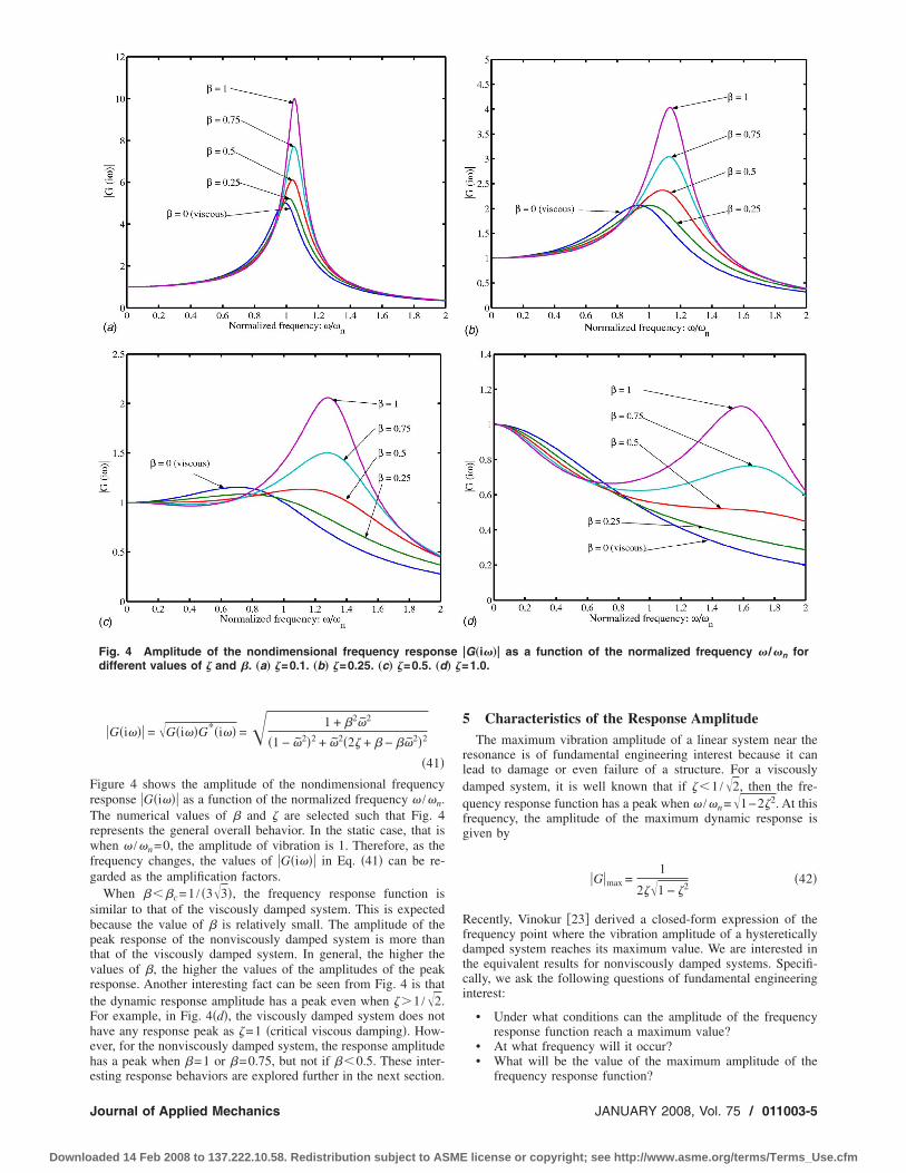
�G�i�� = G�i��G*�i�� = 1 + �2�2

�1 − �2�2 + �2�2� + � − ��2�2

�41�igure 4 shows the amplitude of the nondimensional frequencyesponse �G�i�� as a function of the normalized frequency � /�n.he numerical values of � and � are selected such that Fig. 4

epresents the general overall behavior. In the static case, that ishen � /�n=0, the amplitude of vibration is 1. Therefore, as the

requency changes, the values of �G�i�� in Eq. �41� can be re-arded as the amplification factors.

When ��c=1 / �33�, the frequency response function isimilar to that of the viscously damped system. This is expectedecause the value of � is relatively small. The amplitude of theeak response of the nonviscously damped system is more thanhat of the viscously damped system. In general, the higher thealues of �, the higher the values of the amplitudes of the peakesponse. Another interesting fact can be seen from Fig. 4 is thathe dynamic response amplitude has a peak even when ��1 /2.or example, in Fig. 4�d�, the viscously damped system does notave any response peak as �=1 �critical viscous damping�. How-ver, for the nonviscously damped system, the response amplitudeas a peak when �=1 or �=0.75, but not if �0.5. These inter-

Fig. 4 Amplitude of the nondimensional frequency responsdifferent values of � and �. „a… �=0.1. „b… �=0.25. „c… �=0.5. „d

sting response behaviors are explored further in the next section.



5 Characteristics of the Response AmplitudeThe maximum vibration amplitude of a linear system near the

resonance is of fundamental engineering interest because it canlead to damage or even failure of a structure. For a viscouslydamped system, it is well known that if �1 /2, then the fre-quency response function has a peak when � /�n=1−2�2. At thisfrequency, the amplitude of the maximum dynamic response isgiven by

�G�max =1

2�1 − �2�42�

Recently, Vinokur �23� derived a closed-form expression of thefrequency point where the vibration amplitude of a hystereticallydamped system reaches its maximum value. We are interested inthe equivalent results for nonviscously damped systems. Specifi-cally, we ask the following questions of fundamental engineeringinterest:

• Under what conditions can the amplitude of the frequencyresponse function reach a maximum value?

• At what frequency will it occur?• What will be the value of the maximum amplitude of the

�G„i�…� as a function of the normalized frequency � /�n for1.0.

e

frequency response function?

JANUARY 2008, Vol. 75 / 011003-5


A

fe

F

o

A

t

Te

UD

a

Asi�nfb

0

Downlo

5.1 The Frequency for the Maximum Responsemplitude. For notational convenience, denoting

x = �2 =�2

�n2 �43�

rom Eq. �41�, the amplitude of the dynamic response can bexpressed as

�G�2 =1 + �2x

�1 − x�2 + x�2� + � − �x�2 �44�

or the maximum value of �G�, we set

��G�2

�x= 0 �45�

r

2x2�2 − 2�2x − 2�3�x2 − �4x2 + �4x3 − 1 + x + 2�2 + 2�� − 4�x�

��1 − x�2 + x�2� + � − �x�2�2

= 0 �46�

t the solution point, it is also required that

�2�G�2

�x2 0 �47�

hat in turn implies satisfying

3�6x5 + �9�4 − 12��5 − 6�6�x4 + �9�2 + 12�2�4 − 18�4 − 40�3�

+ 12��5 + 3�6�x3 + �60�2�2 + 9�4 + 3 + 60�3� − 24��

− 18�2�x2 + �9�2 − 24�3� − 48�3� + 12�2 + 36�� − 6

− 72�2�2�x + 3 + 4�3� − 16�2 − 12�� + 20�2�2 + 32�3�

+ 16�4 0 �48�

he numerator of Eq. �46� is a cubic equation in x and can bexpressed as

y

11003-6 / Vol. 75, JANUARY 2008


x3 + �j=0

2

cjxj = 0 �49�

where

c0 =2�� + 2�2 − 1

�4 c1 =1 − 2�2 − 4��

�4 c2 =2 − 2�� − �2

�2

�50�The three roots of Eq. �49� can either be all real or one real andone complex conjugate pair. The nature of the roots depends onthe discriminant, which can be obtained from the constants

Qx =3c1 − c2

2

9= −

1

9�4 �1 + 2�� + �2�2 �51�

and

Rx =9c2c1 − 27c0 − 2c2

3

54

=1

27�6 �8�3�3 + �12�4 − 15�2��2 + �− 15�3 − 21� + 6�5��

+ 3�4 + 3�2 + 1 + �6� �52�as

Dx = Qx3 + Rx

2 = −�

27�11�16�4�4 + �13�3 + 40�5��3

+ �18�4 + 36�6 − 18�2��2 + �− 13� − 12�3 + 15�5 + 14�7��

+ 2 + 8�2 + 12�4 + 2�8 + 8�6� �53�

If Dx�0, then Eq. �49� has one complex conjugate pair and onlyone real solution. It turns out that when Dx�0, the real solution isalways negative and, therefore, is not of interest in this study.However, when Dx0, all the roots of Eq. �49� become real. Wedefine an angle � as

cos�� = �Rx/− Qx3� =

8�3�3 + �12�4 − 15�2��2 + �6�5 − 15�3 − 21�� + 3�4 + 3�2 + 1 + �6

�1 + �2 + 2��3 �54�

sing �, the three real solutions of Eq. �49� can be given usingickson’s formula �24� as

x1 = 2− Qx cos��

3� − c2/3 �55�

x2 = 2− Qx cos�2� + �

3� − c2/3 �56�

nd

x3 = 2− Qx cos�4� + �

3� − c2/3 �57�

mong the above three solutions, we need to choose a positiveolution that also satisfies Eq. �48�. From numerical calculations,t turns out that only x1 in Eq. �55� satisfies the condition in Eq.48�. Substituting Qx from �51� and c2 from �50� into Eq. �55�, theormalized excitation frequency for which the amplitude of therequency response function reaches its maximum value is given

xmax =1

3�2 ��1 + 2�� + �2��2 cos��/3� + 1� − 3 �58�

For convenience, we define the notation �max as

xmax =�max

2

�n2 �59�

we have

�max =�n

��1 + 2�� + �2��2 cos��/3� + 1�/3 − 1 �60�

This is the extension of the well known result for viscouslydamped systems for which �max=�n

1−2�2.Figure 5 shows the contours of �max /�n obtained from Eq.

�60�, as a function of � and �. The value of �max is the frequencywhere the amplitude of the frequency response function reachesits maximum value.

For a better understanding, Fig. 5 is divided into three regions.In region A where ��0.5 and � is small, �max /�n1. This im-plies that in this parameter region, the frequency at which theamplitude of the frequency response function reaches its maxi-
mum appears below the system’s natural frequency. Contour line 0


s�dpoi�rCdCtc

etvThaFtmvrTts

Ae

f�

a

Fsq

J

Downlo

eparates the region B from A and C. In region B, ��0.5 and �

1 /2 and the amplitude of the frequency response functionoes not have any maximum value. This implies that within thisarameter region, it is not possible to find a positive real solutionf the cubic Eq. �49� and the system response decays gradually, asn 4�d� for �=0 and �=0.25. The shaded portion inside region Bshown before in Figs. 2 and 3� corresponds to the parameteregion where the system cannot have any oscillatory motions.learly, within this overdamped region, it is not possible for theynamic response amplitude to reach a maximum value. In region, where ��1 and ��0.5, observe that �max /�n�1. The con-

our plots in Fig. 5 also show a general trend that �max /�n in-reases for increasing values of � and �.

An interesting contour line in Fig. 5 is line 1. For these param-ter combinations of � and �, the frequency at which the ampli-ude of the frequency response function reaches the maximumalue coincides exactly with the undamped natural frequency.his surprising observation implies that the system may beeavily damped ��0.5�, but still can have a peak at �n, for someppropriate values of �. Another interesting fact observed fromig. 5 is that there exist a critical value of �, say �mL, below which

he amplitude of the frequency response will always have a maxi-um value for any values of �. Similarly, there is also a critical

alue of �, say �mU, above which the amplitude of the frequencyesponse will always have a maximum value for any values of �.he explanation of these observations, including the derivation of

he exact values of �mL and �mU, are considered in the next sub-ections.

5.1.1 Critical Parameter Values for the Maximum Responsemplitude. Suppose a general complex solution of Eq. �49� isxpressed as

x = � + i� �61�

or arbitrary � ,��R. Substituting x from the above equation in49� and separating the real and imaginary parts, we have

− 2�4�3 + �4�3� + 2�4 − 4�2��2 + �6�4�2 − 2 + 4�2 + 8��

− 4�� − �4�3� + 2�4 − 4�2��2 − 4�2 + 2 = 0 �62�

ig. 5 Contours of the normalized excitation frequency corre-ponding to the maximum value of the amplitude of the fre-uency response function �max/�n as a function of � and �

nd



− 6�4�2� + �− 8��2 + 8��3� + 4��4�� + 2�4�3 + 4��2 + 8��

− 2� = 0 �63�

Eliminating � from Eqs. �62� and �63� and substituting �=0 �be-cause we are interested only in the real solution� in the resultingequation, after some algebra one has

M��,�� = 0 �64�

where

M��,�� = 16�3�3 + �24�4 − 3�2��2 + �12�5 − 15� − 3�3�� + 2

+ 6�2 + 6�4 + 2�6 �65�

The parameters � and � must satisfy Eq. �64� in order to have areal solution. Therefore, in view of Fig. 5, the values of �mU and�mL can be obtained from the following optimization problems,respectively:

�mU: max � subject to M��,�� = 0 �66�

and

�mL: min � subject to M��,�� = 0 �67�

First, consider the constrained optimization problem in Eq. �66�.Using the Lagrange multiplier �1, we construct the Lagrangian

L1��,�� = � + �1M��,�� 68�

The optimization problem shown in Eq. �66� can be solved bysetting

�L1

��= 0 �69a�

and

�L1

��= 0 �69b�

Differentiating the Lagrangian in Eq. �68�, the above two condi-tions result

�1�48�3�2 + �− 6�2 + 48�4�� − 15� + 12�5 − 3�3� = 0 �70�and

1 + �1�48�2�3 + �− 6� + 96�3��2 + �− 15 + 60�4 − 9�2�� + 12�

+ 24�3 + 12�5� = 0 �71�

Because the Lagrange multiplier �1 cannot be zero, solving Eq.�70� one has

� = −1 + �2

2��72a�

or

� =5 − 4�2

8��72b�

Ignoring the first solution, which is always negative, and substi-tuting �= �5−4�2� /8� in the constraint Eq. �64� and simplifyingwe have

�4 + 2�2 − 11/16 = 0 �73�There is only one feasible solution to the above equation, whichcan be obtained as

�mU = 1233 − 4 = 0.5468 �74�

For this value of �, the value of � can be obtained from Eq. �72b�as

�mU = 34�123 − 6�/11 = 0.8695 �75�

The point ��mU ,�mU� is shown by a dot in Fig. 5. From this plot,
it can be observed that if ��mU, then there always exists a
JANUARY 2008, Vol. 75 / 011003-7


ds

l

wd

F

Tcffs

o

i

pdf

�pqtics

ots

FsqE�tE

0

Downlo

riving frequency for which the amplitude of the frequency re-ponse function will reach a maximum value.

The value of �mL can be obtained from the optimization prob-em �67� by constructing the Lagrangian

L2��,�� = � + �2M��,�� 76�

here �2 is the Lagrange multiplier. Following a similar proce-ure, it can be shown that the optimal value of � is given by

�mL = 125 − 1 = 0.5559 �77�

or this value of �, the value of � can be obtained as

�mL = 1225 − 4 = 0.3436 �78�

he point ��mL ,�mL� is shown by a dot in Fig. 5. From this plot, itan be observed that if ��mL, then there always exists a drivingrequency for which the amplitude of the frequency responseunction will reach a maximum value. From the preceding discus-ions, we have the following fundamental results:

THEOREM 5.1. The amplitude of the frequency response functionf a nonviscously damped oscillator can reach a maximum value

f �125−1 or ��

1233−4.

THEOREM 5.2. If �125−1 or ��

1233−4, then the am-

litude of the frequency response function of a nonviscouslyamped oscillator reaches a maximum value when the drivingrequency �=�n��1+2��+�2��2 cos�� /3�+1� /3−1�� /�.

5.1.2 Parameter Relationships for �max=�n. The contour linemax /�n=1 in Fig. 5 is of special interest. For these particulararameter combinations, the maximum amplitude of the fre-uency response function of the damped system occurs exactly athe undamped natural frequency. This surprising fact occurs onlyn a nonviscously damped system and it is not possible for vis-ously damped systems. For a more detailed analysis, Fig. 6 againhows the contours of �max /�n when �1 and �1.

In Fig. 6, when �=0, then �max /�n can be equal to 1 if andnly if �=0 �that is, when the system is undamped�. The condi-ions for �max /�n=1 can be obtained by enforcing xmax=1. Thus,

ig. 6 Contours of the normalized excitation frequency corre-ponding to the maximum value of the amplitude of the fre-uency response function, �max/�n, as a function of � and �.quations corresponding to �max/�n=0 „dashed line… andmax/�n=1 „dotted line… are shown in the figure. These equa-

ions are valid in the region A only. The function � is defined inq. „81….

ubstituting x=1 in Eq. �49� and considering that ��0, we have

11003-8 / Vol. 75, JANUARY 2008


� + �3 − � = 0 �79�

Solving this, the required condition can be given by

� = ��1 + �2� �80�

when � is known, or

� = ��2 − 12�/6� where � = 3 108� + 1212 + 81�2 �81�

when � is known. Equation �80� is plotted in Fig. 6. The samecurve can also be obtained by plotting Eq. �81�. One interestingfact emerging from Fig. 6 is that beyond certain values of � and �,the maximum dynamic response amplitude cannot occur at�max /�n=1. To obtain these limiting values, we substitute � fromEq. �80� into the condition of real solution given in Eq. �64�. Aftersome algebra, the resulting equation becomes

16�12 + 72�10 + 105�8 + 45�6 − 15�4 − 9�2 + 2 = 0 �82�

The only positive real solution of the above equation is

� = 1/2 �83�

Substituting this value � in Eq. �80�, one obtains

� = 5/8 �84�

The point �5 /8,1 /2� is shown in Fig. 6 by a dot. From this dia-gram, it is clear that �max /�n can be equal to one, if and only if�5 /8 and �1 /2. When xmax=1, the maximum value of theamplitude of the frequency response function can be obtainedfrom Eq. �44� as

�G�xmax=1 =1 + �2

2��85�

From this discussion, we have the following useful results:THEOREM 5.3. The maximum amplitude of the frequency re-

sponse function (if it exists) of a nonviscously damped oscillatorwill occur below the undamped natural frequency if and only if�5 /8 and �1 /2.

THEOREM 5.4. The maximum amplitude of the frequency re-sponse function (if it exists) of a nonviscously damped oscillatorwill occur above the undamped natural frequency if ��5 /8 or��1+�2� and ��1 /2 or �� 2−12� /6�.

Another curious feature of Fig. 6 is the flatness of �max /�naround the contour line 1. This implies that for a wide range ofparameter combinations, it is possible to observe a damped reso-nance very close to the undamped natural frequency. For a vis-cously damped system, this can happen only if the damping isvery small ��0.05�. But for a nonviscously damped system, thiscan happen even when � is as large as 0.6.

It was shown that the amplitude of the frequency response func-tion cannot reach a maximum value for some combinations of �and � �the parameter region B in Figs. 5 and 6�. Consideringsmall values of � and � so that ��mL and ��mL, we aim toderive a simple analytical expression for the existence of �G�max.Because x= �2, the condition for existence of the maximum am-plitude of the frequency response function can be expressed as

xmax � 0 �86�

Therefore, the critical condition can be obtained by substitutingx=0 in Eq. �49� as

1 − 2�� − 2�2 = 0 �87�

Solving this equation for �, the condition for existence of �G�maxcan be expressed by

� 12 �2 + �2 − �� 88�

when



Fs�Ts

w

TWw�a

oc−

Tftm�fTgfvu�fcrpsonm

Ff

J

Downlo

� 1225 − 4 �89�

or the special case when only viscous damping is present, sub-tituting �=0 in Eq. �88�, one obtains the required condition as1 /2, which is well known for viscously damped systems.his condition can alternatively be expressed in terms of � byolving Eq. �87� for � as

� 1 − 2�2

2��90�

hen

� 125 − 1 �91�

he validity of Eqs. �88� and �90� can be verified from Fig. 6.hen ��mL and ��mL, Eqs. �88� and �90� match perfectlyith the zero line obtained from the expression of xmax in Eq.

58�. Observe that these equations become invalid when ��mLnd ��mL. From this discussion, we have the following result:

THEOREM 5.5. If �125−1 and �

1225−4, the amplitude

f the frequency response function of a nonviscously damped os-illator can reach a maximum value if and only if � �2+�2

�� /2 or � �1−2�2� /2�.

5.2 The Amplitude of the Maximum Dynamic Response.he maximum value of the amplitude of the frequency response

unction is a useful quantity because it can be related to the struc-ural failure and design. Figure 7 shows the contours of the maxi-

um amplitude of the normalized frequency response functionG�max as a function of � and �. The values of �G�max are calculatedrom Eq. �44� by substituting xmax from Eq. �58� in place of x.his diagram is divided into four regions for discussions. In re-ion A, where ��mL, the amplitude of the frequency responseunction of the system will always have a maximum value. Thealues of �G�max are higher for smaller values of �, as expected. Aseful fact to be noted is that for a fixed value of �, the value of

G�max is higher for higher values of �. This can also be verifiedrom Fig. 4. This fact may have undesirable consequences, espe-ially if � is large. In region B, the amplitude of the frequencyesponse function does not have a maximum value. The shadedortion inside region B �shown before in Figs. 2 and 3� corre-ponds to the parameter region, where the system cannot have anyscillatory motions. Clearly, within this overdamped region, it isot possible for the dynamic response amplitude to reach a maxi-

ig. 7 Contours of the maximum amplitude of the normalizedrequency response function �G�max as a function of � and �

um value. In region C where ��mU, the amplitude of the



frequency response function of the system will always have amaximum value, but the value of the maximum response is lessthan 1. In region D, observe that ��mU, but unlike region C, thevalue of the maximum response is more than 1. In general, for afixed value of �, the values of �G�max increase with the increasingvalues of �. The numerical values of �G�max in regions C and Dare, however, smaller compared to those in region A. From thisdiscussion, we have the following general result:

THEOREM 5.6. For a given value of �, the maximum amplitudeof the frequency response function �if it exists� of a nonviscouslydamped oscillator increases with increasing values of �.

The contour line “1” in Fig. 7 is of special interest because�G�max�1 implies that the maximum dynamic response amplitudeis more than the static response. For the parameter combinationsin the left side of the contour line 1, the amplitude of the maxi-mum dynamic response is always greater than 1. In the the regionto the right, the amplitude of the maximum dynamic response isless than the static response amplitude of the system. The exactparameter combinations for which �G�max is more than 1 is con-sidered next.

Substituting xmax from Eq. �58� in the expression of �G�2 in Eq.�44�, we can obtain the expression of �G�max

2 . Equating the result-ing expression to 1 and simplifying, we have

�8�3�3 + �12�2 + 12�4��2 + �12�3 + 6� + 6�5�� + 3�2 + 1 + �6

+ 3�4��8 cos3��/3� − 12 cos2��/3�� + 18�8�2�2 + �− 2�5 + 4�

+ 4�3�� − �4 − �6�cos��/3� + 32�3�3 + �48�4 + 12�2��2

+ �− 48� + 6�5 − 24�3�� + 4 + 3�4 − 5�6 + 12�2 = 0 �92�

This is a cubic equation in cos�� /3� and it can be solved exactlyto obtain

cos��/3� =1 − �� − �2/21 + �2 + 2��

�93�

or

cos��/3� =�2 + 2�� + �1 ± 3��/4

1 + �2 + 2��94�

where

� = 4�4 + 4�2 − 8�� + 1 �95�

Among the above three solutions, any one of the two solutionsgiven in Eq. �94� turns out be more useful. In order to obtain therelationship between � and � so that �G�max=1, it is required torelate the expression of cos�� /3� in Eq. �94� to the expression ofcos�� in Eq. �54�. Using the identity

cos�� = 4 cos3��/3� − 3 cos��/3� �96�

and substituting the expression of cos�� from Eq. �54� andcos�� /3� from Eq. �94�, we have

4�4� − ��2 + �2� − 4�2� − 8�4 − 2�� − 4�3 − � − 2�3� − 4�5

− �� = 0 �97�

or

� = −�8�4 + 2�� + 4�5 + 4�3 + � − 16�2�

4�2� + �4�2 − 2�� + 2�3 + ��98�

Equating the right-hand sides of Eqs. �95� and �98� and simplify-ing we have

16�4�2 + �14� − 8�5 + 24�3��3 + �− 4�2 − 8�4 − 2 − 16�6��2

− �9� + 14�3 + 8�7 + 12�5�� + 1 + 5�2 + 8�4 + 4�6 = 0

�99�

The two real and positive solutions of � of the preceding equation
are given by
JANUARY 2008, Vol. 75 / 011003-9


o

IETdEt�F

if

qb

Wtmvr

T

Sc

F

qb

tc

6F

npfodws

�mc

So

T

0

Downlo

� = �2 + �2 − ��/2 �100�r

� = �4�4 + 4�2 + 1�/8� �101�

f the expression of cos�� in Eq. �93� was used in place of that inq. �94�, then one would obtain only the condition in Eq. �100�.he expression of cos�� in Eq. �94� was selected because it pro-uces more general results. Interestingly, the condition given inq. �100� was also identified as the condition for the existence of

he maximum value of the frequency response function in Eq.88�. The value of � given in Eqs. �100� and �101� are shown in

ig. 7. Equation �100� is valid when �1225−4 and Eq. �101�

s valid when ��1225−4. From this analysis, we have the

ollowing fundamental result:THEOREM 5.7. The maximum amplitude of the normalized fre-

uency response function of a nonviscously damped oscillator wille more than 1 if and only if � �2+�2−�� /2 when �

1225−4 and � �4�4+4�2+1� /8� when ��

1225−4.

From this result, one practical question that naturally arises is,hat is the critical value of � below which the maximum ampli-

ude of the normalized frequency response function will always beore than 1? To answer this question, we look for the minimum

alue of � given by Eq. �101�. Differentiating Eq. �101� withespect to �, the optimal value can be obtained from

4�2 + 12�4 − 1

8�2 = 0 �102�

he only real and positive solution of this equation is

� =16

�103�

ubstituting this value of � in Eq. �101�, the optimal value of �an be obtained as

� = 26/9 �104�rom this discussion we have the following theorem:THEOREM 5.8. The maximum amplitude of the normalized fre-

uency response function of a nonviscously damped oscillator wille more than 1 if �26 /9.The converse statement of Theorem 5.8 is, however, not always

rue. The value of �G�max can be more than 1 even if ��26 /9, asan be seen in region C in Fig. 7.

Simplified Analysis of the Frequency ResponseunctionDynamic characteristics of the frequency response function of a

onviscously damped SDOF system have been elucidated in therevious section. The frequency at which the amplitude of therequency response function reaches its maximum value can bebtained from Eq. �58�. Although this is an exact expression, it isifficult to gain much physical insight due to its complexity. Here,e derive some simple expressions considering that � and � are

mall.In Fig. 6, it was noted that for a wide range of values of � and

, the amplitude of the frequency response function reaches itsaximum value when the normalized excitation frequency is

lose to 1. For this reason, we assume that

xmax = 1 − � �105�

ubstituting this in place of x in Eq. �49� and simplifying, onebtains:

�4�3 + �− 2�4 + 2�3� − 2�2��2 + ��4 + 2�2 − 4�3� − 4�� + 1��

+ 2�� + 2�3� − 2�2 = 0 �106�

his is a cubic equation in �, which needs to be solved to obtain

11003-10 / Vol. 75, JANUARY 2008


the frequency where �G�2 reaches its maximum value. Since � isexpected to be small for small values of � and �, neglecting thecoefficients associated with �2 and �3 in Eq. �106� and solving theresulting linear equation we obtain

� �2�2 − 2��1 + �2�

�1 + �2��1 + �2 − 4��107�

Substituting � in Eq. �105�, the frequency corresponding to themaximum value of the amplitude of the frequency response func-tion can be approximately obtained as

�max = xmax =�max

�n�1 −

2�2 − 2��1 + �2��1 + �2��1 + �2 − 4��

�108�For the special case when only viscous damping is present, sub-stituting �=0 in Eq. �108�, one obtains �max=1−2�2, which iswell known for viscously damped systems.

Substituting x=xmax from �105� into the expression of �G�2 inEq. �44� and retaining only up to quadratic terms in �, one has

�G�max2 �

1 + �2 − �2�

4�2 + �4�� − 4�2�� + ��2 + 1 − 4��2 �109�

Substituting � from �107� into the preceding equation and retain-ing only up to cubic terms in �, one has

�G�max �1

2� �1 + �2�

�1 + 2�2��1 − 4�� + �3 − 2�2��2 − 6�3��

�1 − 2�� − �2��110�

For the special case when only viscous damping is present, sub-stituting �=0 in Eq. �110� results in the exact corresponding ex-pression �G�max=1 / �2�1−�2�, as given in Eq. �42�. To verify theaccuracy of the approximate formulas �108� and �110�, we calcu-late the percentage error with respect to the exact solutions ob-tained in the previous section. The percentage error is calculated,for example, as

100 ��max�exact − ��max�approx

��max�exact

�111�

Figures 8 and 9, respectively, show the contours of percentageerrors arising due to the use of approximate Eqs. �108� and �110�.

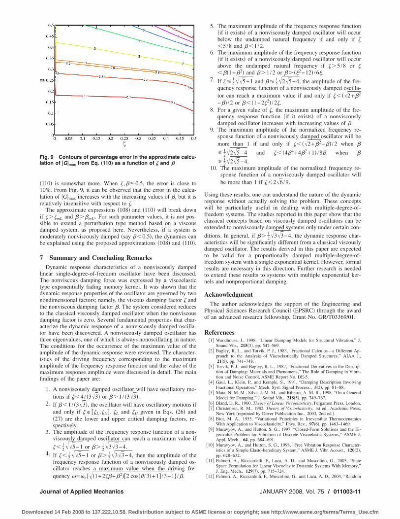
For �max calculated from Eq. �108�, the error is less than 2%

Fig. 8 Contours of percentage error in the approximate calcu-lation of �max/�n from Eq. „108… as a function of � and �

when � ,�0.5. The error in the calculation of �G�max from Eq.



�1lr

isdmb

7

lTtdnttdattTaiamfi

Fl

J

Downlo

110� is somewhat more. When � ,��0.5, the error is close to0%. From Fig. 9, it can be observed that the error in the calcu-ation of �G�max increases with the increasing values of �, but it iselatively insensitive with respect to �.

The approximate expressions �108� and �110� will break downf ��mL and ��mU. For such parameter values, it is not pos-ible to extend a perturbation type method based on a viscousamped system, as proposed here. Nevertheless, if a system isoderately nonviscously damped �say �0.5�, the dynamics can

e explained using the proposed approximations �108� and �110�.

Summary and Concluding RemarksDynamic response characteristics of a nonviscously damped

inear single-degree-of-freedom oscillator have been discussed.he nonviscous damping force was expressed by a viscoelastic

ype exponentially fading memory kernel. It was shown that theynamic response properties of the oscillator are governed by twoondimensional factors; namely, the viscous damping factor � andhe nonviscous damping factor �. The system considered reduceso the classical viscously damped oscillator when the nonviscousamping factor is zero. Several fundamental properties that char-cterize the dynamic response of a nonviscously damped oscilla-or have been discovered. A nonviscously damped oscillator hashree eigenvalues, one of which is always nonoscillating in nature.he conditions for the occurrence of the maximum value of themplitude of the dynamic response were reviewed. The character-stics of the driving frequency corresponding to the maximummplitude of the frequency response function and the value of theaximum response amplitude were discussed in detail. The mainndings of the paper are:

1. A nonviscously damped oscillator will have oscillatory mo-tions if �4 / �33� or ��1 / �33�.

2. If �1 / �33�, the oscillator will have oscillatory motions ifand only if �� L ,�U�. �L and �U given in Eqs. �26� and�27� are the lower and upper critical damping factors, re-spectively.

3. The amplitude of the frequency response function of a non-viscously damped oscillator can reach a maximum value if

�125−1 or ��

1233−4.

4. If �125−1 or ��

1233−4, then the amplitude of the

frequency response function of a nonviscously damped os-cillator reaches a maximum value when the driving fre-

2

ig. 9 Contours of percentage error in the approximate calcu-ation of �G�max from Eq. „110… as a function of � and �

quency �=�n� �1+2��+� ��2 cos�� /3�+1� /3−1 /�.



5. The maximum amplitude of the frequency response function�if it exists� of a nonviscously damped oscillator will occurbelow the undamped natural frequency if and only if �5 /8 and �1 /2.

6. The maximum amplitude of the frequency response function�if it exists� of a nonviscously damped oscillator will occurabove the undamped natural frequency if ��5 /8 or ��1+�2� and ��1 /2 or �� 2−12� /6�.

7. If �125−1 and �

1225−4, the amplitude of the fre-

quency response function of a nonviscously damped oscilla-tor can reach a maximum value if and only if � �2+�2

−�� /2 or � �1−2�2� /2�.8. For a given value of �, the maximum amplitude of the fre-

quency response function �if it exists� of a nonviscouslydamped oscillator increases with increasing values of �.

9. The maximum amplitude of the normalized frequency re-sponse function of a nonviscously damped oscillator will bemore than 1 if and only if � �2+�2−�� /2 when �

1225−4 and � �4�4+4�2+1� /8� when �

�1225−4.

10. The maximum amplitude of the normalized frequency re-sponse function of a nonviscously damped oscillator willbe more than 1 if �26 /9.

Using these results, one can understand the nature of the dynamicresponse without actually solving the problem. These conceptswill be particularly useful in dealing with multiple-degree-of-freedom systems. The studies reported in this paper show that theclassical concepts based on viscously damped oscillators can beextended to nonviscously damped systems only under certain con-

ditions. In general, if ��1233−4, the dynamic response char-

acteristics will be significantly different from a classical viscouslydamped oscillator. The results derived in this paper are expectedto be valid for a proportionally damped multiple-degree-of-freedom system with a single exponential kernel. However, formalresults are necessary in this direction. Further research is neededto extend these results to systems with multiple exponential ker-nels and nonproportional damping.

AcknowledgmentThe author acknowledges the support of the Engineering and

Physical Sciences Research Council �EPSRC� through the awardof an advanced research fellowship, Grant No. GR/T03369/01.

References�1� Woodhouse, J., 1998, “Linear Damping Models for Structural Vibration,” J.

Sound Vib., 215�3�, pp. 547–569.�2� Bagley, R. L., and Torvik, P. J., 1983, “Fractional Calculus—a Different Ap-

proach to the Analysis of Viscoelastically Damped Structures,” AIAA J.,21�5�, pp. 741–748.

�3� Torvik, P. J., and Bagley, R. L., 1987, “Fractional Derivatives in the Descrip-tion of Damping: Materials and Phenomena,” The Role of Damping in Vibra-tion and Noise Control, ASME Report No. DE-5.

�4� Gaul, L., Klein, P., and Kemple, S., 1991, “Damping Description InvolvingFractional Operators,” Mech. Syst. Signal Process., 5�2�, pp. 81–88.

�5� Maia, N. M. M., Silva, J. M. M., and Ribeiro, A. M. R., 1998, “On a GeneralModel for Damping,” J. Sound Vib., 218�5�, pp. 749–767.

�6� Bland, D. R., 1960, Theory of Linear Viscoelasticity, Pergamon Press, London.�7� Christensen, R. M., 1982, Theory of Viscoelasticity, 1st ed., Academic Press,

New York �reprinted by Dover Publication Inc., 2003, 2nd ed.�.�8� Biot, M. A., 1955, “Variational Principles in Irreversible Thermodynamics

With Application to Viscoelasticity,” Phys. Rev., 97�6�, pp. 1463–1469.�9� Muravyov, A., and Hutton, S. G., 1997, “Closed-Form Solutions and the Ei-

genvalue Problem for Vibration of Discrete Viscoelastic Systems,” ASME J.Appl. Mech., 64, pp. 684–691.

�10� Muravyov, A., and Hutton, S. G., 1998, “Free Vibration Response Character-istics of a Simple Elasto-hereditary System,” ASME J. Vibr. Acoust., 120�2�,pp. 628–632.

�11� Palmeri, A., Ricciardelli, F., Luca, A. D., and Muscolino, G., 2003, “StateSpace Formulation for Linear Viscoelastic Dynamic Systems With Memory,”J. Eng. Mech., 129�7�, pp. 715–724.

�12� Palmeri, A., Ricciardelli, F., Muscolino, G., and Luca, A. D., 2004, “Random

JANUARY 2008, Vol. 75 / 011003-11


0

Downlo

Vibration of Systems With Viscoelastic Memory,” J. Eng. Mech., 130�9�, pp.1052–1061.

�13� Wagner, N., and Adhikari, S., 2003, “Symmetric State-Space Formulation fora Class of Non-viscously Damped Systems,” AIAA J., 41�5�, pp. 951–956.

�14� Adhikari, S., and Wagner, N., 2003, “Analysis of Asymmetric Non-viscouslyDamped Linear Dynamic Systems,” ASME J. Appl. Mech., 70�6�, pp. 885–893.

�15� Cremer, L., and Heckl, M., 1973, Structure-Borne Sound, 2nd ed., Springer-Verlag, Berlin, Germany �translated by E. E. Ungar�.

�16� Adhikari, S., and Woodhouse, J., 2001, “Identification of Damping: Part, 2,Non-viscous Damping,” J. Sound Vib., 243�1�, pp.63–88.

�17� McTavish, D. J., and Hughes, P. C., 1993, “Modeling of Linear ViscoelasticSpace Structures,” ASME J. Vibr. Acoust., 115, pp. 103–110.

�18� Adhikari, S., 2002, “Dynamics of Non-viscously Damped Linear Systems,” J.Eng. Mech., 128�3�, pp. 328–339.

11003-12 / Vol. 75, JANUARY 2008


�19� Adhikari, S., 2005, “Qualitative Dynamic Characteristics of a Non-viscouslyDamped Oscillator,” Proc. R. Soc. London, Ser. A, 461,�2059�, pp. 2269–2288.

�20� Adhikari, S., and Woodhouse, J., 2003, “Quantification of Non-viscous Damp-ing in Discrete Linear Systems,” J. Sound Vib., 260�3�, pp. 499–518.

�21� Abramowitz, M., and Stegun, I. A., 1965, Handbook of Mathematical Func-tions, With Formulas, Graphs, and Mathematical Tables, Dover Publications,New York.

�22� Muller, P., 2005, “Are the Eigensolutions of a 1-d.o.f. System With Viscoelas-tic Damping Oscillatory or Not?,” J. Sound Vib., 285�1–2�, pp. 501–509.

�23� Vinokur, R., 2003, “The Relationship Between the Resonant and Natural Fre-quency for Non-viscous Systems,” J. Sound Vib., 267, pp. 187–189.

�24� Dickson, L. E., 1898, “A New Solution of the Cubic Equation,” Am. Math.Monthly, 5, pp. 38–39.



dynamic response characteristics of a …engweb.swan.ac.uk/~adhikaris/fulltext/journal/ft35.pdfmu¨...

Documents