dynamic routing for flying ad hoc networks dynamic routing for flying ad hoc networks stefano...

1

Dynamic Routing for Flying Ad Hoc NetworksStefano Rosati, Member, IEEE, Karol Kruzelecki, Member, IEEE, Gregoire Heitz, Dario

Floreano, Senior Member, IEEE, and Bixio Rimoldi, Fellow, IEEE

Abstract—This paper reports experimental results onself-organizing wireless networks carried by small flyingrobots. Flying ad hoc networks (FANETs) composed ofsmall unmanned aerial vehicles (UAVs) are flexible, in-expensive and fast to deploy. This makes them a veryattractive technology for many civilian and military appli-cations. Due to the high mobility of the nodes, maintaininga communication link between the UAVs is a challengingtask. The topology of these networks is more dynamicthan that of typical mobile ad hoc networks (MANETs)and of typical vehicle ad hoc networks (VANETs). As aconsequence, the existing routing protocols designed forMANETs partly fail in tracking network topology changes.

In this work, we compare two different routing algo-rithms for ad hoc networks: optimized link-state routing(OLSR), and predictive-OLSR (P-OLSR). The latter is anOLSR extension that we designed for FANETs; it takesadvantage of the GPS information available on board. Tothe best of our knowledge, P-OLSR is currently the onlyFANET-specific routing technique that has an availableLinux implementation. We present results obtained byboth Media Access Control (MAC) layer emulations andreal-world experiments. In the experiments, we used atestbed composed of two autonomous fixed-wing UAVs anda node on the ground. Our experiments evaluate the linkperformance and the communication range, as well as therouting performance.

Our emulation and experimental results show that P-OLSR significantly outperforms OLSR in routing in thepresence of frequent network topology changes.

I. INTRODUCTION

In the case of a calamitous event, when ordinarycommunication infrastructure is out of service or simplynot available, a group of small flying robots can providea rapidly deployable and self-managed ad hoc Wi-Finetwork to connect and coordinate rescue teams on theground. Networks of small unmanned aerial vehicles1

(UAVs) can also be employed for wildfire monitoring

S. Rosati, K. Kruzelecki, and B. Rimoldi are with the MobileCommunications Laboratory (LCM), Swiss Federal Institute of Tech-nology (EPFL), Lausanne, Switzerland. G. Heitz and D. Floreanoare with Laboratory of Intelligent Systems (LIS), EPFL, Lausanne,Switzerland. Email: {stefano.rosati, karol.kruzelecki, gregoire.heitz,dario.floreano, bixio.rimoldi}@epfl.ch

1Small UAVs are also knows as micro-air vehicles (MAVs)

[1], border surveillance [2], and for extending ad hocnetworks on the ground [3], [4], [5].

The recent technological progress in electronics andcommunication systems, especially due to the the wide-spread availability of low-cost micro-embedded com-puters and Wi-Fi radio interfaces, has paved the wayfor the creation of inexpensive flying ad hoc networks(FANETs), however, a challenging networking problemarises.

As pointed out in [6], FANETs are a special case ofmobile ad hoc networks (MANETs) characterized bya high degree of mobility. In a FANET, the topologyof the network can change more frequently than in atypical MANET or vehicle ad hoc network (VANET).As a consequence, the network routing becomes a crucialtask [7], [8]. The network routing algorithms, which havebeen designed for MANETs, such as BABEL [9] or theoptimized link-state routing (OLSR) protocol [10], [11],fail to follow the evolution of the network topology. Itis possible to bypass this problem by considering starnetworks with static routing [12]. However, star archi-tectures restrict the operative area of groups of UAVs,because the nodes cannot fly out of the communicationrange of the control center. In this paper, we focus onpartially-connected mesh ad hoc networks that enablethe UAVs to use multi-hop communication to extendthe operative area. In this case, the problem of highlydynamic routing must be faced.

A few methods for overcoming the problem caused bya rapidly changing network topology have recently beenproposed: Guo at al. [13] present a UAV-aided cross-layer routing protocol (UCLR) that aims at improvingthe routing performance of a ground MANET networkwith aid from one UAV. In [14], the authors propose theuse of directional antennas and two cross-layer schemes,named Intelligent Media Access Control (MAC), andDirectional-OLSR. The latter is an extension of OLSR.The choice of the route is based on flight information(such as attitude variations, pitch, roll and yaw). Theauthors report only OPNET simulation results. Benzaidet al [15], [16] present an OLSR extension denoted Fast-OLSR that aims at meeting the need for highly dynamicrouting in MANETs composed of fast-moving and slow-moving nodes. This extension increases the rate of the

arX

iv:1

406.

4399

v3 [

cs.N

I] 1

8 M

ar 2

015

2

Hello messages only for the nodes that move faster thana given speed. If the fast-moving nodes are a smallpercentage of the network’s nodes, the additional over-head is limited. Otherwise, if the network is composedmainly of UAVs, the overhead grows significantly. In[17], we present an extension to the OLSR protocolnamed predictive-OLSR (P-OLSR). The key idea of thisextension is to use GPS information available on boardand to weigh the expected transmission count (ETX)metric by a factor that takes into account the directionand the relative speed between the UAVs.

In this paper, we present field experiments that com-pare P-OLSR against OLSR. The experiments involvedtwo UAVs and a ground station. The carriers were fixed-wing autonomous planes called eBees and developedby SenseFly [18]. Each plane carried an embeddedcomputer-on-module and an 802.11n radio interface.The field-test results show that P-OLSR can followrapid topology changes and provide a reliable multi-hop communication in situations where OLSR mostlyfails. In order to assess the behavior of P-OLSR inlarger networks, we carried out MAC-layer emulationsconsidering a network composed of 19 UAVs. To thebest of our knowledge, P-OLSR is currently the onlyFANET-specific routing technique that has an availableLinux implementation. The open-source software of theP-OLSR daemon can be downloaded from [19].

The rest of the paper is organized as follows. InSection II, we highlight the differences between OLSRand P-OLSR. In Section III, we specify the modifiedstructure of the Hello messages and describe the im-plementation of the P-OLSR daemon. In Section IV,we describe the testbed and in Section V we describethe experiments and present the results. In Section VI,we present the MAC-layer emulation we used to assessthe P-OLSR performance in larger networks. Finally, wedraw our conclusions in Section VII.

II. ROUTING FOR FLYING AD HOC NETWORKS

In [12], Frew and Brown analyze the networking forsystems of small UAVs. They characterize four differentnetwork architectures: direct-link, satellite, cellular, andad hoc (also called mesh networking). The direct-link andthe satellite architecture are star networks where all theUAVs are either directly connected to the ground controlor to a satellite connected to the ground control. This is asimple network architecture: it does not require dynamicrouting, because all the nodes are directly connectedwith the control center. The nodes require, however,long-range (terrestrial or satellite) links, hence they arenot suitable for small UAVs. Furthermore, UAV-to-UAVcommunication is inefficiently routed through the control

center, even if the nodes operate the same area. Thismight cause traffic congestion in the control center,which is also a weakness of the system in case of attack.

In the cellular architecture, the UAVs are connectedto a cellular system with many base stations scattered onthe ground. UAVs can do a handover between differentbase stations during the flight. This architecture does notneed a single vulnerable control center. However, theoperating area of the UAVs is limited by the cellularnetwork extension. In the case of a catastrophic event,the UAV system can be deployed only if the cellularnetwork is present and functioning in the area.

In the ad hoc architecture, every node can act asa router. These networks are also know as FANETs:they have no central infrastructure, therefore, they arevery robust against isolated attacks or node failures.Moreover, as these networks do not rely on any externalsupport they can be rapidly deployed anywhere. Thesecharacteristics, on one hand, make FANETs the mostsuitable solution for many applications, but on the otherhand, they raise a challenging networking problem.

In fact, due to the rapid and erratic movement of theUAVs, the topology of a FANET can vary rapidly andthe nodes must react by automatically updating theirrouting tables. Therefore, in a FANET it is crucial toemploy a fast and reactive routing procedure. In [17]we show that some of the most popular routing algo-rithms for MANETs, such as OLSR and BABEL, failto track the fast topology changes of a FANET. Similarconclusions are also drawn in [7]. For this reason, in[17], we introduce P-OLSR. To predict how the qualityof the wireless links between the nodes is likely toevolve, P-OLSR exploits the GPS information, whichis typically available from the UAV’s autopilot. For thesake of completeness, in this section we briefly report thedefinition of ETX, as well as, the key concepts behindP-OLSR.

A. Link-Quality Estimation

OLSR is currently one of the most popular proactiverouting algorithms for ad hoc networks. It is based onthe link-state routing protocol. The original OLSR designdoes not consider the quality of the wireless link. Theroute selection is based on the hop count metric, whichis inadequate for mobile wireless networks. However,by using the ETX metric [20], the OLSR link-qualityextension enables us to take into account the quality ofthe wireless links. The ETX metric was introduced in[21], and it is defined as

ETX(R) =∑η∈R

ETX(η) =∑η∈R

1

φ(η)ρ(η), (1)

3

where, R is a route between two nodes of the network,and η is a hop of the route R. φ(η) is the forwardreceiving ratio, i. e., the probability that a packet sentthrough the hop η is successfully received. ρ(η) isthe reverse receiving ratio, i.e., the probability that thecorresponding ACK packet is successfully received. Inother words, ETX estimates the expected number oftransmissions (including re-transmissions) necessary todeliver a packet from the source to its final destination.Then OLSR selects the route that has the smallest ETX,which is not necessarily the one with the least numberof hops. If all the hops forming R are errorless (i.e.,φ(η) = ρ(η) = 1) the ETX(R) is equal to the numberof hops of R.

The receiving ratios are typically estimated by link-probe messages. The OLSR link-quality extension usesthe control messages named Hello messages as a link-probe. φ is computed by means of an exponential movingaverage, as follows,{

φl = αhl + (1− α)φl−1φ0 = 0

, 0 ≤ α ≤ 1 , (2)

where

hl =

{1 if the l-th Hello message is received0 otherwise

; (3)

and α is an OLSR parameter, named link-quality aging,that drives the trade-off between the accuracy and re-sponsiveness of the receiving ratio estimation. On onehand, with a greater α, the receiving ratios will beaveraged for a longer time, thus yielding a more stableand reliable estimation. On the other hand, with a lowerα, the system will react faster. Another important OLSRparameter is the Hello Interval (HI) that indicates howfrequently Hello messages are broadcasted.

B. Speed-Weighted ETX

In a FANET the nodes move rapidly, for example, thecruising speed of our flying robots is around 12 metersper second. The network topology changes rapidly, anda wireless link between two UAVs can break suddenly.In these networks, the ETX metric might be inadequate,because it is not reactive enough to follow the link vari-ations. Due to the delay introduced by the exponentialmoving average, a node notices that a certain wirelesslink has broken with a non-negligible delay. Therefore,for a significant amount of time, it will continue routingpackets on a link that is actually broken.

To solve this problem, we modify the ETX metric totake into account the position and the direction of theUAV, with respect to its neighbors. The ETX(η) metric

of the hop η between the nodes i and j is weighed by afactor that accounts for the relative speed between i andj as follows:

ETX(η) =ev

i,j` β

φ(η)ρ(η), (4)

where vi,j` is the relative speed between nodes i and j,and β is a non-negative parameter.

If the nodes i and j move closer to each other, therelative speed is negative, thus the ETX will be weightedby a factor smaller than 1. Otherwise, if the nodes iand j move apart from each other, the relative speedis positive, thus the ETX will be weighted by a factorgreater than 1. In other words, a hop between two nodesthat move closer to each other is preferred rather thana hop between two nodes that move apart, even if theyhave the same values of φ and ρ.

In order to compute the speed-weighted ETX, we as-sume that every node knows the position of its neighbors.As illustrated in the Appendix III, to distribute the GPScoordinates across the network we add a field to theHello messages.

The instantaneous relative velocity between i and j attime ti is computed as

vi,j` =di,j` − d

i,j`−1

t` − t`−1, (5)

where, t` and t`−1 are, the arrival time of the last andsecond to last Hello message. di,j` and di,j`−1 are thecorresponding distances between the nodes i and j. Asthe GPS positions are subject to errors, and gusts ofwind can perturb the motion of the UAVs, it is preferableto average the instantaneous speed using a exponentialmoving average as follows:

{vi,j` = γvi,j` + (1− γ)vi,j`−1vi,j0 = 0

, 0 ≤ γ ≤ 1 , (6)

where γ is a P-OLSR parameter. Acting on the P-OLSRparameter β and γ, we can optimize the routing selectionto the cruising speed of the UAVs, and to the chosen HI.

Fixed-wing UAVs require forward motion for flying.They also require a minimum air-speed and turningradius. Therefore the direction of the UAV is a goodindicator for predicting its position in the near future, andthen to foresee how the link quality is likely to evolve.

III. IMPLEMENTATION DETAILS

In order to implement the P-OLSR protocol, we forkedan open-source implementation of OLSR called OLSRd[22]. In the modified version, the Hello messages are

4

augmented to contain position information. Thus, everynode knows its neighbors’ positions and can computethe corresponding ETX according to (4).

A. OLSRd with Link-Quality Extension

OLSRd uses link-quality sensing and ETX metricsthrough the so-called link-quality extension [20]. It re-places the hysteresis mechanism of the OLSR protocolwith link-quality sensing algorithms that are intended tobe used with ETX-based metrics. To do so, the link-quality extension uses the OLSR Hello messages toprobe link quality and to advertise link-specific qualityinformation, (i.e. receiving ratios, φ and ρ), in addition todetecting and advertising neighbors. Likewise, it includesthe link-quality information also in OLSR TopologyControl (TC) messages that are to be distributed to thewhole network. Clearly the modified messages are notRFC-compliant anymore because they include new fieldsfor link-quality information. Therefore, all the nodes inthe network have to use the link-quality extension.

B. P-OLSRd Implementation

To implement P-OLSR, we have to share the coordi-nates (i.e. longitude, latitude, and altitude) of each nodewith its neighbors. This is done through the Hello mes-sages. Subsequently, each node uses its neighbors’ co-ordinates to compute the corresponding relative speeds,and share them across the whole network via both Helloand TC messages.

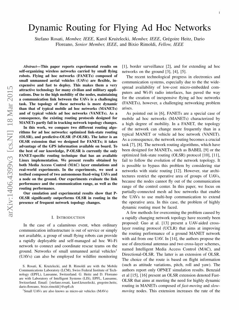
Fig. 1 depicts the structure of the original Hellomessage in OLSRd. The first block of 8 bytes carriesinformation about the node itself. Note that in this blockthere are 3 reserved bytes that are not used by the OLSRdaemon and are filled with zeros. Then, a block of 8bytes is appended for each neighbor seen by the node.This block is formatted as follows: 4 bytes are for theIP address of the neighbor, 1 byte is for the forwardreceiving ratio2 φ(η′), 1 byte is for the reverse receivingratio ρ(η′), and 2 bytes that are not used, hence filledwith zeros.

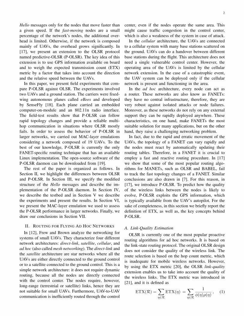
Fig. 2 depicts the modified structure of the Hello mes-sage. We highlight in gray the fields that were added ormodified. The first part of the message contains 16 bytesinstead of 8. It contains the latitude and the longitude,formatted as single-precision floating-point numbers that

2η′ is the hop between the node the is producing the Hello messageand its neighbor.

9

Neighbor interface address

Link Code Link Message SizeReserved

0 1 2 3 4 5 6 70 21 3byte byte byte byte

Reserved Htime Willingness0 1 2 3 4 5 6 7 0 1 2 3 4 5 6 7 0 1 2 3 4 5 6 7

φ(η′) ρ(η′) Reserved


φ(η′′) ρ(η′′) Reserved

......

...

Fig. 1. Format of the original (i.e. OLSRd) Hello message.

...



Altitude Htime Willingness0 1 2 3 4 5 6 7 0 1 2 3 4 5 6 7 0 1 2 3 4 5 6 7

φ(η′) ρ(η′) vi,j′

ℓ (rel. speed)


Latitude

φ(η′′) ρ(η′′) vi,j′′

ℓ (rel. speed)


...

...

Longitude

Fig. 2. Format of the modified (i.e. P-OLSRd) Hello message.


Reserved

0 1 2 3 4 5 6 7 0 1 2 3 4 5 6 7 0 1 2 3 4 5 6 7

advertise neighbor main address

Reserved

......

...

ANSN

φ(η′′) ρ(η′′)


Reservedφ(η′) ρ(η′)

Fig. 3. Format of the original (i.e. OLSRd) Topology Control message. ANSN stands for Advertised Neighbor Sequence Number.


Reserved

0 1 2 3 4 5 6 7 0 1 2 3 4 5 6 7 0 1 2 3 4 5 6 7


ρ(η′′)

......

...

ANSN

vi,j′′

ℓ (rel. speed)



ℓ (rel. speed)

ρ(η′′)

Fig. 4. Format of the modified (i.e. P-OLSRd) Topology Control message.

November 4, 2014 DRAFT


9








......

...


...





ℓ (rel. speed)


Latitude

φ(η′′) ρ(η′′) vi,j′′

ℓ (rel. speed)


...

...

Longitude



Reserved

0 1 2 3 4 5 6 7 0 1 2 3 4 5 6 7 0 1 2 3 4 5 6 7


Reserved

......

...

ANSN

φ(η′′) ρ(η′′)





Reserved

0 1 2 3 4 5 6 7 0 1 2 3 4 5 6 7 0 1 2 3 4 5 6 7


ρ(η′′)

......

...

ANSN

vi,j′′

ℓ (rel. speed)



ℓ (rel. speed)

ρ(η′′)




occupy 4 bytes each3. The altitude is formatted as a 16-bit fixed-point number that replaces the 2 reserved bytesnot used by the OLSR daemon. Similarly to the originalHello message, a block of 8 bytes is appended for eachneighbor seen by the node. The only difference hereis that we use the 2 empty bytes to communicate theaveraged relative speed between the nodes. The speed isformatted as a 16-bit fixed-point number.

The size difference between the original and themodified Hello message is 8 bytes, independently of thenumbers of nodes in the network. The Hello messageis encapsulated into a UDP datagram that, in turn, isencapsulated in an IP packet and then into a 802.11frame. For medium and large networks, the additional8 bytes constitute a negligible overload compared to thetotal size of the frame.

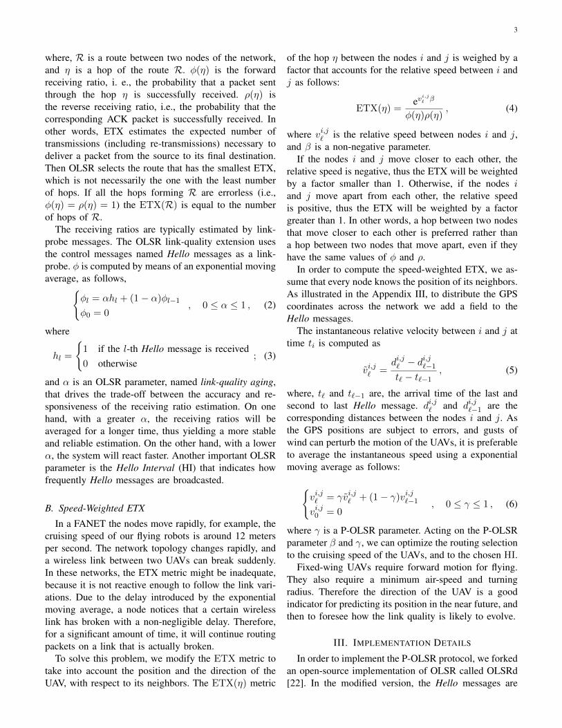
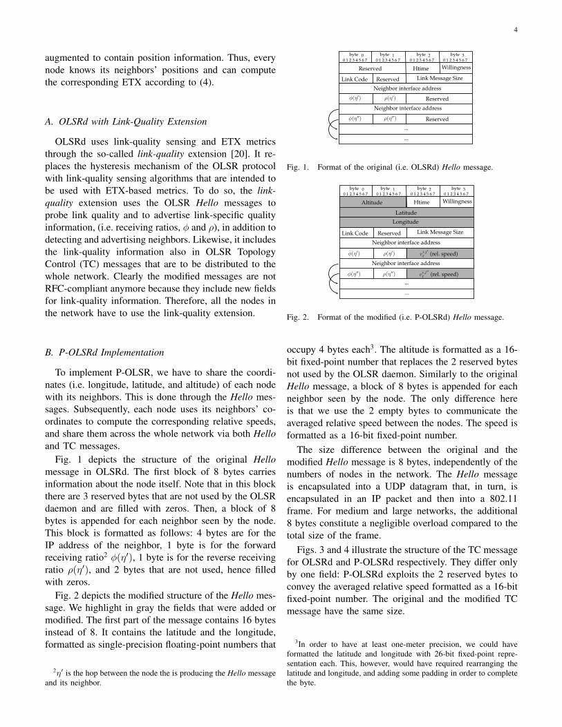
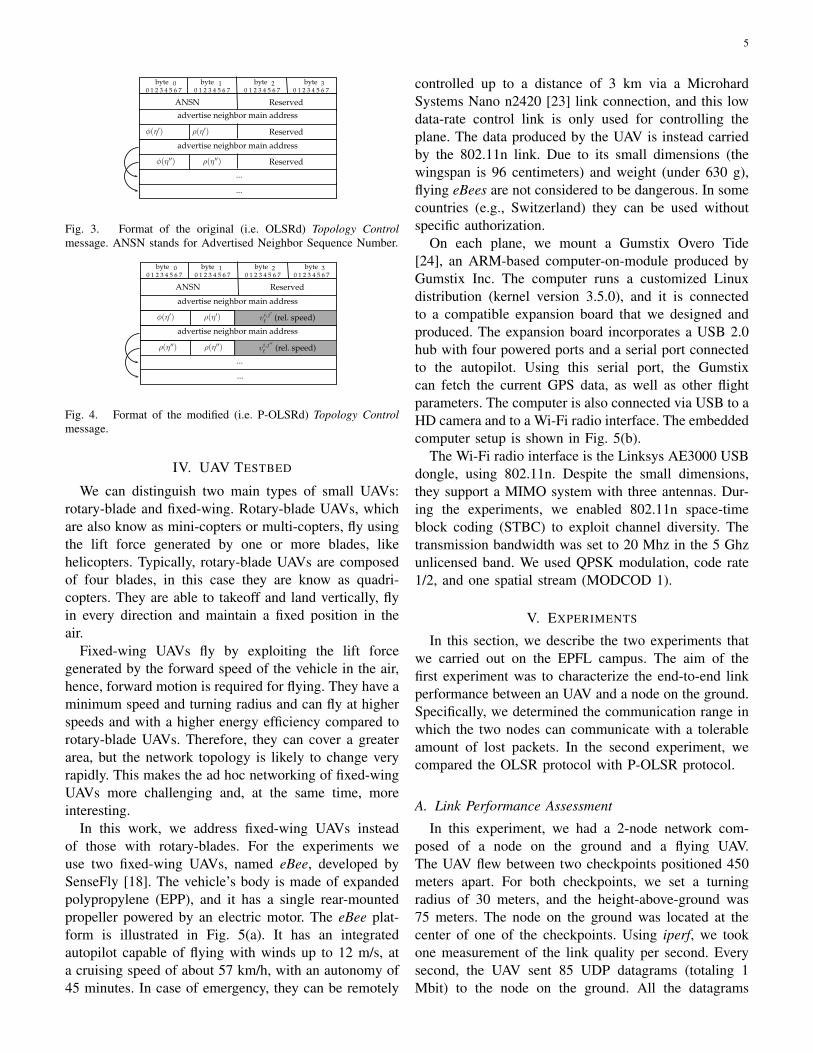
Figs. 3 and 4 illustrate the structure of the TC messagefor OLSRd and P-OLSRd respectively. They differ onlyby one field: P-OLSRd exploits the 2 reserved bytes toconvey the averaged relative speed formatted as a 16-bitfixed-point number. The original and the modified TCmessage have the same size.

3In order to have at least one-meter precision, we could haveformatted the latitude and longitude with 26-bit fixed-point repre-sentation each. This, however, would have required rearranging thelatitude and longitude, and adding some padding in order to completethe byte.

5

9








......

...


...





ℓ (rel. speed)


Latitude

φ(η′′) ρ(η′′) vi,j′′

ℓ (rel. speed)


...

...

Longitude



Reserved

0 1 2 3 4 5 6 7 0 1 2 3 4 5 6 7 0 1 2 3 4 5 6 7


Reserved

......

...

ANSN

φ(η′′) ρ(η′′)





Reserved

0 1 2 3 4 5 6 7 0 1 2 3 4 5 6 7 0 1 2 3 4 5 6 7


ρ(η′′)

......

...

ANSN

vi,j′′

ℓ (rel. speed)



ℓ (rel. speed)

ρ(η′′)



Fig. 3. Format of the original (i.e. OLSRd) Topology Controlmessage. ANSN stands for Advertised Neighbor Sequence Number.

9








......

...


...





ℓ (rel. speed)


Latitude

φ(η′′) ρ(η′′) vi,j′′

ℓ (rel. speed)


...

...

Longitude



Reserved

0 1 2 3 4 5 6 7 0 1 2 3 4 5 6 7 0 1 2 3 4 5 6 7


Reserved

......

...

ANSN

φ(η′′) ρ(η′′)





Reserved

0 1 2 3 4 5 6 7 0 1 2 3 4 5 6 7 0 1 2 3 4 5 6 7


ρ(η′′)

......

...

ANSN

vi,j′′

ℓ (rel. speed)



ℓ (rel. speed)

ρ(η′′)



Fig. 4. Format of the modified (i.e. P-OLSRd) Topology Controlmessage.

IV. UAV TESTBED

We can distinguish two main types of small UAVs:rotary-blade and fixed-wing. Rotary-blade UAVs, whichare also know as mini-copters or multi-copters, fly usingthe lift force generated by one or more blades, likehelicopters. Typically, rotary-blade UAVs are composedof four blades, in this case they are know as quadri-copters. They are able to takeoff and land vertically, flyin every direction and maintain a fixed position in theair.

Fixed-wing UAVs fly by exploiting the lift forcegenerated by the forward speed of the vehicle in the air,hence, forward motion is required for flying. They have aminimum speed and turning radius and can fly at higherspeeds and with a higher energy efficiency compared torotary-blade UAVs. Therefore, they can cover a greaterarea, but the network topology is likely to change veryrapidly. This makes the ad hoc networking of fixed-wingUAVs more challenging and, at the same time, moreinteresting.

In this work, we address fixed-wing UAVs insteadof those with rotary-blades. For the experiments weuse two fixed-wing UAVs, named eBee, developed bySenseFly [18]. The vehicle’s body is made of expandedpolypropylene (EPP), and it has a single rear-mountedpropeller powered by an electric motor. The eBee plat-form is illustrated in Fig. 5(a). It has an integratedautopilot capable of flying with winds up to 12 m/s, ata cruising speed of about 57 km/h, with an autonomy of45 minutes. In case of emergency, they can be remotely

controlled up to a distance of 3 km via a MicrohardSystems Nano n2420 [23] link connection, and this lowdata-rate control link is only used for controlling theplane. The data produced by the UAV is instead carriedby the 802.11n link. Due to its small dimensions (thewingspan is 96 centimeters) and weight (under 630 g),flying eBees are not considered to be dangerous. In somecountries (e.g., Switzerland) they can be used withoutspecific authorization.

On each plane, we mount a Gumstix Overo Tide[24], an ARM-based computer-on-module produced byGumstix Inc. The computer runs a customized Linuxdistribution (kernel version 3.5.0), and it is connectedto a compatible expansion board that we designed andproduced. The expansion board incorporates a USB 2.0hub with four powered ports and a serial port connectedto the autopilot. Using this serial port, the Gumstixcan fetch the current GPS data, as well as other flightparameters. The computer is also connected via USB to aHD camera and to a Wi-Fi radio interface. The embeddedcomputer setup is shown in Fig. 5(b).

The Wi-Fi radio interface is the Linksys AE3000 USBdongle, using 802.11n. Despite the small dimensions,they support a MIMO system with three antennas. Dur-ing the experiments, we enabled 802.11n space-timeblock coding (STBC) to exploit channel diversity. Thetransmission bandwidth was set to 20 Mhz in the 5 Ghzunlicensed band. We used QPSK modulation, code rate1/2, and one spatial stream (MODCOD 1).

V. EXPERIMENTS

In this section, we describe the two experiments thatwe carried out on the EPFL campus. The aim of thefirst experiment was to characterize the end-to-end linkperformance between an UAV and a node on the ground.Specifically, we determined the communication range inwhich the two nodes can communicate with a tolerableamount of lost packets. In the second experiment, wecompared the OLSR protocol with P-OLSR protocol.

A. Link Performance Assessment

In this experiment, we had a 2-node network com-posed of a node on the ground and a flying UAV.The UAV flew between two checkpoints positioned 450meters apart. For both checkpoints, we set a turningradius of 30 meters, and the height-above-ground was75 meters. The node on the ground was located at thecenter of one of the checkpoints. Using iperf, we tookone measurement of the link quality per second. Everysecond, the UAV sent 85 UDP datagrams (totaling 1Mbit) to the node on the ground. All the datagrams

6

batteryHD camera

pitot tube control link

motor & propeller

802.11 dongle

embedded

computer

(a) SenseFly eBee with HD camera, Linksys AE3000 USBdongle, and Gumstix computer-on-module.

Gumstix

computer

customized

expansion board

power supply

& serial port

to the autopilot

(b) Computer and expansion board in the rear compartment ofthe UAV.

Fig. 5. UAV platform used in the experiments.

received with a delay greater than 5 seconds wereconsidered lost. We also counted as correctly received thedatagrams that arrived out of order (provided that theirdelay was smaller than 5 seconds). This is what can betolerated by a video streaming, where the video is playedwith a 5-second delay. Every second, we computed thedatagram loss rate (DLR), which is the ratio between thedatagram lost and their total number.

The results are reported in Fig. 6. The black crossesrepresent the DLR measured at a given distance. Thedashed line represents the corresponding non-linearleast-square regression function. The function that weuse as a model is

1

1 + e−(p1+p2d), (7)

where d is the distance in meters and p1 and p2 are thecoefficients to be estimated. Using a non-linear fittingmethod, we compute the value of p1 and p2, thus yieldingthe best fitting in the least square sense. They are p1 =8.9 and p2 = 0.025.

0 100 200 300 400 5000

0.2

0.4

0.6

0.8

1

distance [m]

DL

R

regression functionexperimental DLR

Fig. 6. Experimental datagram loss rate vs. distance. The blackcrosses are the DLR measured values, and the dashed red line is thecorresponding non-linear least-square regression function.

0

50

100

150

200

250

Num

ber

ofm

easu

rem

ents

Number of measurements

0 100 200 300 400 5000

0.2

0.4

0.6

0.8

1

distance [m]

DL

RAverage DLR

Fig. 7. Average datagram loss rate vs. distance. The blue barsrepresent the number of measurements per distance interval. Thegreen solid line is the average DLR.

In Fig. 7, we quantize the distance between transmitterand receiver with a bin width of 20 meters. For each binwe compute the average DLR. The resulting curve isplotted in green. We also report the number of measure-ments per bin.

As we can see from these results, the connection isgood when the distance is shorter than 250 meters. Inthis region, the observed DLR is always lower than 0.2.We observe a transition from 250 meters to 300, wherethe DLR can be as high as 1, but on average it is lowerthan 0.3. When the distance is greater than 300 meters,the connection degrades significantly and the DLR isoften close to 1. The average DLR is 0.5 at 350 meters.We observe some sporadic cases of a good connectioneven when the distance is greater than 400 meters.

7

B. Routing Performance Assessment

In the second experiment, we compared the routingperformance of OLSR with link-quality extension andP-OLSR. For both OLSR and P-OLSR, we set the HIequal to 0.5 seconds. This value is a good trade-offbetween the amount of overhead and the reactivity-speedof the algorithm. Using the default HI value, which inOLSRd is equal to 2 seconds, the algorithm would havebeen too slow to pursue the topology changes. As P-OLSR exploits the GPS information to estimate the link-quality evolution, it could work also with a longer HI.Nevertheless, for the sake of fairness, we use the samevalue for both algorithms.

We set the link-quality aging, α, equal to 0.2 forOLSR, and to 0.05 for P-OLSR. This parameter controlsthe trade-off between the accuracy and the responsive-ness of the receiving ratio estimation. As before, as P-OLSR can predict the link-quality evolution, it can workwith a smaller α, yielding a more accurate estimationof the receiving ratio. OLSR, on the contrary, needs angreater aging value to increase its responsiveness, at theexpense of accuracy. The other P-OLSR parameters wereβ = 0.2, and γ = 0.04.

We had a network of three nodes: one fixed destinationon the ground (node 1), one flying UAV source (Node 2),and one flying UAV relay (Node 3). Node 1 was on theterrace of the BC building on the EPFL campus (latitude:46.51843◦ N; longitude: 6.561591◦ E). The UAV source,Node 2 flew following a straight trajectory of 600 meterswest from Node 1, then it returned to the starting point.The UAV relay, Node 3, followed a circular trajectoryof radius 30 meters and centered at 250 meters westfrom Node 1. Both the UAVs flew about 75 metersabove the ground, and the terrace of the BC building isapproximately 10 meters above the ground. The actualtrajectories followed by the planes are illustrated in Fig.8.

We performed 10 loops for each routing algorithms.The loop-time is affected by the weather conditions,especially the wind. During our experiment, the eBeetook on average 120 seconds to complete a loop. Thetime difference between the fastest and the slowest loopwas around 10 seconds. In each loop, Node 2 changedits routing to reach Node 1, from a direct connectionto a two-hop connection, and vice versa. Therefore thenetwork topology was expected to change two timesduring the each loop.

Fig. 9 shows the evolution of the DLR during the 10runs. For OLSR, we notice some peaks of the DLR thatcorrespond to the moments when the routing algorithmhas to switch from the direct link to a two-hop. This

−650 −600 −550 −500 −450 −400 −350 −300 −250 −200 −150 −100 −50 0 50−50

0

50

[2][3]

[1]

x[m]

y[m

]

UAV Source UAV Relay Destination

Fig. 8. Trajectories of the UAVs during the network field experi-ments.

0 100 200 300 400 500 600 700 800 900 1,000 1,100 1,2000

0.2

0.4

0.6

0.8

1

time [s]

DL

R

EmulationOLSR

P-OLSRExperiments

OLSRP-OLSR

Fig. 9. Evolution of the average DLR. Dashed lines report theresults of MAC-layer emulations, solid lines report the results offield experiments.

happens because OLSR takes several seconds to detectthat a wireless direct-link is broken. This translates intoan interruption of the service. P-OLSR, however, reactspromptly to topology changes. As we can see from thefield-test results, P-OLSR is able to predict a change inthe topology and reacts before the previous link breaks.The DLR peaks that we see on the P-OLSR results aredue to the fading of the wireless channels rather than toincorrect routing.

VI. MAC-LAYER EMULATIONS WITH LARGER

NETWORKS

In this section, we examine the behavior of P-OLSRoperating on larger FANETs. When many UAVs areinvolved, field experiments become expensive. For thisreason, we analyze the performance of P-OLSR via anetwork emulation platform that integrates all the testbedaspects.

A. Emulation Platform

In order to analyze the routing performance inmedium/large FANETs, we developed the emulationplatform illustrated in Fig. 10. It creates a Linux con-tainer (LXC) for each node of the network. The nodesare connected using a MAC-layer real-time emulatorcalled Extendable Mobile Ad-Hoc Network Emulator(EMANE). EMANE is an open-source framework, de-veloped primarily by Naval Research Laboratory [25].The MAC and the physical layers are emulated, whereasthe remaining layers use the real software implemen-tations used by the Linux machine. For a propagation

816

Application

Transport

Network OLSR, Predictive-OLSR

TCP, UDP

iperf

MAC

Physical

runningon

LX

Cs

802.11 EMANE model

802.11 TGn model UAVs’ positions

Experiments Emulations

IEEE 802.11

runningon

Gum

Stixs GPS Error model

Fig. 10. Emulation platform.

VI. MAC-LAYER EMULATIONS WITH LARGER NETWORKS

In this section, we examine the behavior of P-OLSR operating on larger FANETs. When

many UAVs are involved, field experiments become expensive. For this reason, we analyze the

performance of P-OLSR via a network emulation platform that integrates all the testbed aspects.

A. Emulation Platform

In order to analyze the routing performance in medium/large FANETs, we developed the

emulation platform illustrated in Fig. 10. It creates a Linux container (LXC) for each node of

the network. The nodes are connected using a MAC-layer real-time emulator called Extendable

Mobile Ad-Hoc Network Emulator (EMANE). EMANE is an open-source framework, developed

primarily by Naval Research Laboratory [25]. The MAC and the physical layers are emulated,

whereas the remaining layers use the real software implementations used by the Linux machine.

For a propagation channel model, we use the IEEE 802.11 TGn model D, defined in [26]. This

model was proposed for outdoor environments with line-of-sight conditions. EMANE imports

the positions of the UAVs from log files and uses them to compute the pathloss for each link.

These log files can be obtained from real-flight data logs, or by a flight simulator that reproduces

realistic flight conditions. Before passing the UAV’s position to the P-OLSR daemon, we add an

error to take into account imperfect GPS receivers. We model GPS errors following the statistical

characterization of GPS error provided in [27].


Fig. 10. Emulation platform.

channel model, we use the IEEE 802.11 TGn model D,defined in [26]. This model was proposed for outdoorenvironments with line-of-sight conditions. EMANE im-ports the positions of the UAVs from log files and usesthem to compute the pathloss for each link. These logfiles can be obtained from real-flight data logs, or by aflight simulator that reproduces realistic flight conditions.Before passing the UAV’s position to the P-OLSR dae-mon, we add an error to take into account imperfect GPSreceivers. We model GPS errors following the statisticalcharacterization of GPS error provided in [27].

B. Emulation Results

We carried out two network emulation campaigns. Inthe first one, we reproduced the conditions we had inthe experiments. This was done to test the emulator. Weused the positions reported in the log files of the actualexperiments. Fig. 9 shows emulation results (dashedlines) side-by-side with the experimental results (solidlines) for OLSR and for P-OLSR. The emulation resultsmatch with the experimental ones.

In the second emulation campaign, we assessed thebehavior of P-OLSR in larger networks and we analyzedthe role of various parameters, namely the Hello interval(HI), the link-quality aging (α), and the P-OLSR specificparameters (β and γ). The network consisted of 19moving UAVs. One UAV (Node 2) scanned a rectangulararea of 1200 square meters, by following the trajectoryplotted with a dashed line in Fig. 11. It took 380 secondsto complete the trajectory. The other UAVs (Nodes1, 3, . . . , 19) are uniformly spread within the area. Theycirculated around the respective waypoints, reproducingthe behaviour of actual fixed-wing UAVs. The radius ofthe circular trajectories was 30 meters, the speed was12 m/s and the initial phase was uniformly distributedbetween zero and 2π. The distance between the relayswas such that only the closest neighbors had a directlink. For example, node 10 can communicate directlyonly with Nodes 5, 7, 8, 12, 13, and 15.

−600−400−200 0 200 400 600

−400

−200

0

200

400

600

[7]

[1]

[12]

[17]

[5]

[10]

[15]

[3]

[8]

[13]

[18]

[6]

[11]

[16]

[4]

[9]

[14]

[19]

[2]

x[m]

y[m

]

Relays Destination Source

Fig. 11. Emulations set-up. A network composed of 19 nodes. Node2 is flying with a speed of 12 m/s following the trajectory markerswith red dashed line.

As we did in the experiments, we sent 85 UDPdatagrams per second (totaling 1 Mbit) from Node 2 toNode 1, using iperf. In order to have a more compactrepresentation of the results, we compared the networkperformance in terms of average outage time. We saythat an outage occurs when the DLR becomes greaterthan 0.2. The outage duration of such an event is thelength of the interval during which the DLR stays above0.2. The outage time of a run is the sum of all the outagedurations. In order to average the results, we repeated theemulation 10 times for each configuration.

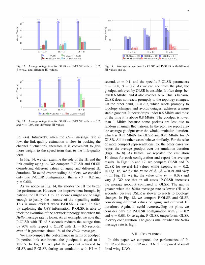
In Figs. 12 and 13 we compare OLSR and P-OLSRfor different durations of the HI while keeping the agingparameter α equal to 0.2. We present several P-OLSRconfigurations: In Fig. 12, we maintain a fixed value ofβ, (β = 0.2) and we vary the speed aging parameter γ. InFig. 13, we fix γ (γ = 0.08) and we vary the value of β.Notice that P-OLSR reduces drastically the outage timecompared to OLSR. In all its configurations, P-OLSRcuts down the outage time by at least 85%. Consideringonly the best performing P-OLSR configurations, theoutage reduction is about 95%, 92%, and 90%, for HIdurations equal to 0.5, 1, and 2 seconds, respectively.

In Fig. 12, we compare P-OLSR configurations fordifferent values of γ. We see that when the HI is short,it is convenient to decrease the value of γ, and viceversa. The reason is that if the Hello message rate islow, it is convenient to have a fast aging of the previousspeed estimates. In Fig. 13, we examine the role of theparameter β. We notice that when the HI is long, it ismore convenient to increase β, meaning that the speedterm has a greater weight in the EXT computation, (see

9

HI = 0.5s HI = 1s HI = 2s0

10

20

30

40

54.8 74.6 112.3

2.4

6

18.6

6.4 6.5

11.612.6

10.4 11.1

Out

age

Tim

e[s]

OLSR P-OLSR(γ = 0.04)

P-OLSR(γ = 0.08) P-OLSR(γ = 0.16)

Fig. 12. Average outage time for OLSR and P-OLSR with α = 0.2,β = 0.2, and different HI values.

HI = 0.5s HI = 1s HI = 2s0

10

20

30

40

54.8 74.6 112.3

2.33.4

21

6.4 6.5

11.6

Out

age

Tim

e[s]

OLSR P-OLSR(β = 0.1) P-OLSR(β = 0.2)

Fig. 13. Average outage time for OLSR and P-OLSR with α = 0.2,and γ = 0.08, and different HI values.

Eq. (4)). Intuitively, when the Hello message rate islow, the link-quality estimation is slow in tracking thechannel fluctuations, therefore it is convenient to givemore weight to the speed term than to the link-qualityterm.

In Fig. 14, we can examine the role of the HI and thelink quality aging, α. We compare P-OLSR and OLSRconsidering different values of aging and different HIdurations. To avoid overcrowding the plots, we consideronly one P-OLSR configuration, that is (β = 0.2 andγ = 0.08).

As we notice in Fig. 14, the shorter the HI the betterthe performance. However the improvement brought byhalving the HI from 1 to 0.5 seconds might not be largeenough to justify the increase of the signalling traffic.This is more evident when P-OLSR is used. In fact,by exploiting the GPS information, P-OLSR is able totrack the evolution of the network topology also when theHello message rate is lower. As an example, we note thatP-OLSR with HI of 2 seconds reduces the outage timeby 80% with respect to OLSR with HI = 0.5 seconds,even if it generates about 1/4 of the Hello messages.

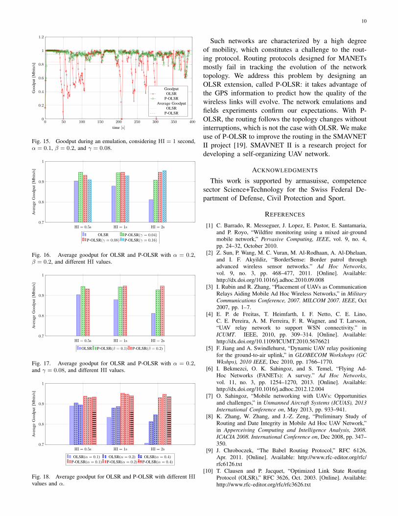
We also compare the performance in terms of goodput.In perfect link conditions, the goodput is equal to 1Mbit/s. In Fig. 15, we plot the goodput achieved byOLSR and P-OLSR during an emulation with HI = 1

HI = 0.5s HI = 1s HI = 2s0

50

100

150

63.8

103.6

156.4

54.8

74.6

112.3

62.167.5

92.6

6 7.3

23.1

6.4 6.511.6

7.6 5.910.1

Out

age

Tim

e[s]

OLSR(α = 0.1) OLSR(α = 0.2) OLSR(α = 0.4)P-OLSR(α = 0.1) P-OLSR(α = 0.2) P-OLSR(α = 0.4)

Fig. 14. Average outage time for OLSR and P-OLSR with differentHI values and α.

second, α = 0.1, and the specific-P-OLSR parametersγ = 0.08, β = 0.2. As we can see from the plot, thegoodput achieved by OLSR is unstable. It often drops be-low 0.6 Mbit/s, and it also reaches zero. This is becauseOLSR does not reacts promptly to the topology changes.On the other hand, P-OLSR, which reacts promptly totopology changes and avoids outages, achieves a morestable goodput. It never drops under 0.6 Mbit/s and mostof the time it is above 0.8 Mbit/s. The goodput is lowerthan 1 Mbit/s because some packets are lost due torandom channels fluctuations. In the plot, we report alsothe average goodput over the whole emulation duration,which is 0.83 Mbit/s for OLSR and 0.95 Mbit/s for P-OLSR. All the other cases behave similarly. For the sakeof more compact representations, for the other cases wereport the average goodput over the emulation duration(Figs. 16-18). As before, we repeated the emulation10 times for each configuration and report the averageresults. In Figs. 16 and 17, we compare OLSR and P-OLSR for several HI values while keeping α = 0.2.In Fig. 16, we fix the value of β, (β = 0.2) and varyγ. In Fig. 17, we fix the value of γ (γ = 0.08) andvary β. We see that in all cases, P-OLSR increasesthe average goodput compared to OLSR. The gap isgreater when the Hello message rate is lower (HI = 2seconds), because OSLR is slower to reacts to topologychanges. In Fig. 18, we compare P-OLSR and OLSRconsidering different values of aging and different HIdurations. Again, to avoid overcrowding the plots, weconsider only the P-OLSR configuration with β = 0.2and γ = 0.08. Once again, P-OLSR outperforms OLSRin every configuration. The gap is smaller when the Hellomessage rate is high.

VII. CONCLUSION

In this paper we compared the performance of P-OLSR and that of OLSR in a FANET composed of smallfixed-wing UAVs.

10

0 50 100 150 200 250 300 350 4000

0.2

0.4

0.6

0.8

1

1.2

[12]

time [s]

Goo

dput

[Mbi

ts/s

]

GoodputOLSR

P-OLSRAverage Goodput

OLSRP-OLSR

Fig. 15. Goodput during an emulation, considering HI = 1 second,α = 0.1, β = 0.2, and γ = 0.08.

HI = 0.5s HI = 1s HI = 2s0.7

0.8

0.9

1

Ave

rage

Goo

dput

[Mbi

ts/s

]

OLSR P-OLSR(γ = 0.04)

P-OLSR(γ = 0.08) P-OLSR(γ = 0.16)

Fig. 16. Average goodput for OLSR and P-OLSR with α = 0.2,β = 0.2, and different HI values.

HI = 0.5s HI = 1s HI = 2s0.7

0.8

0.9

1

Ave

rage

Goo

dput

[Mbi

ts/s

]

OLSR P-OLSR(β = 0.1) P-OLSR(β = 0.2)

Fig. 17. Average goodput for OLSR and P-OLSR with α = 0.2,and γ = 0.08, and different HI values.

HI = 0.5s HI = 1s HI = 2s0.7

0.8

0.9

1

Ave

rage

Goo

dput

[Mbi

ts/s

]

OLSR(α = 0.1) OLSR(α = 0.2) OLSR(α = 0.4)P-OLSR(α = 0.1) P-OLSR(α = 0.2) P-OLSR(α = 0.4)

Fig. 18. Average goodput for OLSR and P-OLSR with different HIvalues and α.

Such networks are characterized by a high degreeof mobility, which constitutes a challenge to the rout-ing protocol. Routing protocols designed for MANETsmostly fail in tracking the evolution of the networktopology. We address this problem by designing anOLSR extension, called P-OLSR: it takes advantage ofthe GPS information to predict how the quality of thewireless links will evolve. The network emulations andfields experiments confirm our expectations. With P-OLSR, the routing follows the topology changes withoutinterruptions, which is not the case with OLSR. We makeuse of P-OLSR to improve the routing in the SMAVNETII project [19]. SMAVNET II is a research project fordeveloping a self-organizing UAV network.

ACKNOWLEDGMENTS

This work is supported by armasuisse, competencesector Science+Technology for the Swiss Federal De-partment of Defense, Civil Protection and Sport.

REFERENCES

[1] C. Barrado, R. Messeguer, J. Lopez, E. Pastor, E. Santamaria,and P. Royo, “Wildfire monitoring using a mixed air-groundmobile network,” Pervasive Computing, IEEE, vol. 9, no. 4,pp. 24–32, October 2010.

[2] Z. Sun, P. Wang, M. C. Vuran, M. Al-Rodhaan, A. Al-Dhelaan,and I. F. Akyildiz, “BorderSense: Border patrol throughadvanced wireless sensor networks.” Ad Hoc Networks,vol. 9, no. 3, pp. 468–477, 2011. [Online]. Available:http://dx.doi.org/10.1016/j.adhoc.2010.09.008

[3] I. Rubin and R. Zhang, “Placement of UAVs as CommunicationRelays Aiding Mobile Ad Hoc Wireless Networks,” in MilitaryCommunications Conference, 2007. MILCOM 2007. IEEE, Oct2007, pp. 1–7.

[4] E. P. de Freitas, T. Heimfarth, I. F. Netto, C. E. Lino,C. E. Pereira, A. M. Ferreira, F. R. Wagner, and T. Larsson,“UAV relay network to support WSN connectivity.” inICUMT. IEEE, 2010, pp. 309–314. [Online]. Available:http://dx.doi.org/10.1109/ICUMT.2010.5676621

[5] F. Jiang and A. Swindlehurst, “Dynamic UAV relay positioningfor the ground-to-air uplink,” in GLOBECOM Workshops (GCWkshps), 2010 IEEE, Dec 2010, pp. 1766–1770.

[6] I. Bekmezci, O. K. Sahingoz, and S. Temel, “Flying Ad-Hoc Networks (FANETs): A survey.” Ad Hoc Networks,vol. 11, no. 3, pp. 1254–1270, 2013. [Online]. Available:http://dx.doi.org/10.1016/j.adhoc.2012.12.004

[7] O. Sahingoz, “Mobile networking with UAVs: Opportunitiesand challenges,” in Unmanned Aircraft Systems (ICUAS), 2013International Conference on, May 2013, pp. 933–941.

[8] K. Zhang, W. Zhang, and J.-Z. Zeng, “Preliminary Study ofRouting and Date Integrity in Mobile Ad Hoc UAV Network,”in Apperceiving Computing and Intelligence Analysis, 2008.ICACIA 2008. International Conference on, Dec 2008, pp. 347–350.

[9] J. Chroboczek, “The Babel Routing Protocol,” RFC 6126,Apr. 2011. [Online]. Available: http://www.rfc-editor.org/rfc/rfc6126.txt

[10] T. Clausen and P. Jacquet, “Optimized Link State RoutingProtocol (OLSR),” RFC 3626, Oct. 2003. [Online]. Available:http://www.rfc-editor.org/rfc/rfc3626.txt

http://dx.doi.org/10.1016/j.adhoc.2010.09.008

http://dx.doi.org/10.1109/ICUMT.2010.5676621

http://dx.doi.org/10.1016/j.adhoc.2012.12.004

http://www.rfc-editor.org/rfc/rfc6126.txt



11

[11] C. Dearlove, T. Clausen, and P. Jacquet, “The OptimizedLink State Routing Protocol version 2,” IETF Draft RFCdraft-ietf-manet-olsrv2-10, 2009. [Online]. Available: http://tools.ietf.org/id/draft-ietf-manet-olsrv2-19.txt

[12] E. W. Frew and T. X. Brown, “Networking Issues forSmall Unmanned Aircraft Systems,” Journal of Intelligent andRobotic Systems, vol. 54, no. 1-3, p. 21, 2008. [Online].Available: http://dx.doi.org/10.1007/s10846-008-9253-2

[13] Y. Guo, X. Li, H. Yousefi’zadeh, and H. Jafarkhani, “UAV-aidedcross-layer routing for MANETs,” in Wireless Communicationsand Networking Conference (WCNC), 2012 IEEE, April 2012,pp. 2928–2933.

[14] A. Alshbatat and L. Dong, “Cross layer design for mobile Ad-Hoc Unmanned Aerial Vehicle communication networks,” inNetworking, Sensing and Control (ICNSC), 2010 InternationalConference on, April 2010, pp. 331–336.

[15] M. Benzaid, P. Minet, and K. Al Agha, “Integrating fastmobility in the OLSR routing protocol,” in Mobile and WirelessCommunications Network, 2002. 4th International Workshopon, 2002, pp. 217–221.

[16] M. Benzaid, P. Minet, and K. Al-Agha, “Analysis and simula-tion of fast-OLSR,” in Vehicular Technology Conference, 2003.VTC 2003-Spring. The 57th IEEE Semiannual, vol. 3, April2003, pp. 1788–1792 vol.3.

[17] S. Rosati, K. Kruzelecki, L. Traynard, and B. Rimoldi, “Speed-Aware Routing for UAV Ad-Hoc Networks,” in 4th Interna-tional IEEE Workshop on Wireless Networking & Control forUnmanned Autonomous Vehicles: Architectures, Protocols andApplications, 2013.

[18] Sensefly eBee. [Online]. Available: http://www.sensefly.com/drones/ebee.html

[19] SMAVNET II website. [Online]. Available: http://smavnet.epfl.ch

[20] olsrd Link Quality Extensions. [Online]. Available: http://www.olsr.org/docs/README-Link-Quality.html

[21] D. S. J. De Couto, D. Aguayo, J. Bicket, and R. Morris, “AHigh-throughput Path Metric for Multi-hop Wireless Routing,”in Proceedings of the 9th Annual International Conferenceon Mobile Computing and Networking, ser. MobiCom ’03.New York, NY, USA: ACM, 2003, pp. 134–146. [Online].Available: http://doi.acm.org/10.1145/938985.939000

[22] Optimized Link State Routing Deamon. [Online]. Available:http://www.olsr.org/

[23] Microhard Systems Inc. Spread Spectrum Wireless Modem.[Online]. Available: http://www.microhardcorp.com/n2420.php

[24] Gumstix Web Page: Overo Tide COM Product overview.[Online]. Available: https://www.gumstix.com/store/app.php/products/257/

[25] Extendable Mobile Ad-hoc Network Emulator (EMANE).[Online]. Available: http://cs.itd.nrl.navy.mil/work/emane/

[26] IEEE P802.11 Wireless LANs, “TGn Channel Models,” IEEEStd 802.11 11-03/940r4, Tech. Rep., 2004.

[27] E. Akim and D. Tuchin, “GPS errors statistical analysis forground receiver measurements,” Keldysh Institute of AppliedMathematics, Russia Academy of Sciences, 2002.

Stefano Rosati (S’07-M’11) is a Post-DocResearch Engineer at the Ecole PolytechniqueFederale de Lausanne (EPFL), Switzerland. Hereceived the Laurea degree (summa cum laude)and Ph.D. degree in Telecommunications Engi-neering from the University of Bologna, Italy,in 2007 and 2011, respectively. From 2007to 2011, he was with the Advanced ResearchCenter for Electronic Systems (ARCES) of

the University of Bologna. In 2010, he was an Intern Engineer atCorporate R&D Department of Qualcomm Inc. (San Diego, CA).In 2011 he joined the Information Processing Group (IPG) and theMobile Communications Laboratory (LCM) at EPFL.

His interests are in various aspects of digital communications, inparticular next-generation cellular communication systems, and bothterrestrial and satellite broadcast networks. His research activities arealso focused on flying ad-hoc networks and self-organizing networksof Unmanned Aerial Vehicles (UAVs). He has authored severalscientific papers and internationals patents regarding these topics.

Karol Kruzelecki (M’09) is a research engi-neer working at EPFL, Lausanne, Switzerland.He received his Msc. Eng. degree in ComputerScience and in Computational Mechanics fromCracow University of Technology, Poland, inSeptember and November 2008 respectively.Between 2008 and 2011 he was working atThe European Organization for Nuclear Re-search (CERN) on the development of auto-

matic build and test system used to improve the software quality andreliability for the Large Hadron Collider beauty experiment (LHCb).In 2012 he joined the Information Processing Group (IPG) and theMobile Communications Laboratory (LCM) of the EPFL.

Gregoire Heitz is an engineer working at theLaboratory of Intelligent System at EPFL sinceSeptember 2012. He obtained a M.Sc in Elec-tronic from the ENSCPE of Lyon (France) in2012. He was working in senseFly SA for hismaster thesis, working on the development of anew flying robot in 2011. His research interestlies in embedded systems development.

http://tools.ietf.org/id/draft-ietf-manet-olsrv2-19.txt

http://tools.ietf.org/id/draft-ietf-manet-olsrv2-19.txt

http://dx.doi.org/10.1007/s10846-008-9253-2

http://www.sensefly.com/drones/ebee.html

http://www.sensefly.com/drones/ebee.html

http://smavnet.epfl.ch

http://smavnet.epfl.ch

http://www.olsr.org/docs/README-Link-Quality.html

http://www.olsr.org/docs/README-Link-Quality.html

http://doi.acm.org/10.1145/938985.939000

http://www.olsr.org/

http://www.microhardcorp.com/n2420.php

https://www.gumstix.com/store/app.php/products/257/

https://www.gumstix.com/store/app.php/products/257/

http://cs.itd.nrl.navy.mil/work/emane/

12

Dario Floreano (SM’06) received the M.A.and Ph.D. degrees from the University of Tri-este, Trieste, Italy, in 1988 and 1995, respec-tively, and the M.S. degree from the Universityof Stirling, Stirling, Scotland, in 1991. Heis Full Professor at the Ecole PolytechniqueFederale de Lausanne, Lausanne, Switzerland,where he is Director of the Laboratory ofIntelligent Systems and Director of the Swiss

National Center of Competence in Robotics. His research interestsare at the convergence of biology, artificial intelligence, and robotics.He authored more than 300 peer-reviewed articles and 3 books onthe topics of evolutionary robotics, bio-inspired artificial intelligence,and biomimetic flying robots, and spun two companies off

Bixio Rimoldi (S’83-M’85-SM’92-F’00) re-ceived his Diploma and his Doctorate fromthe Electrical Engineering department of theEidgenoossische Technische Hochschule inZurich (ETHZ). During 1988-1989 he heldvisiting positions at the University of NotreDame and Stanford. In 1989 he joined the fac-ulty of Electrical Engineering at WashingtonUniversity, St. Louis, and since 1997 he is

a Full Professor at the Ecole Polytechnique Federale de Lausanne(EPFL) and director of the Mobile Communications Lab. He hasspent sabbatical leaves at MIT (2006) and at the University ofCalifornia, Berkeley (2003-2004).

In 1993 he received a US National Science Foundation YoungInvestigator Award. In 2000 he was elected to the grade of Fellowof the IEEE. During the period 2002-2009 he has been on the Boardof Governors of the IEEE Information Theory Society where heserved in several offices including President. He was co-chairmanwith Bruce Hajek of the 1995 IEEE Information Theory Workshop onInformation Theory, Multiple Access, And Queueing (St Louis, MO),and co-chairman with Jim Massey of the 2002 IEEE InternationalSymposium in Information Theory (Lausanne, Switzerland). He wasa member of the editorial board of ”Foundations and Trends onCommunications and Information Theory,” and was an editor ofthe European Transactions on Telecommunications. During 2005and 2006 he was the director of EPFL’s undergraduate program inCommunication Systems.

His interests are in various aspects of digital communications, inparticular information theory, and software-defined radio.

dynamic routing for flying ad hoc networks dynamic routing for flying ad hoc networks stefano...

Documents