dynamic scaling and growth behavior of queuing … · queuing network normalization constants 493...

Dynamic Scaling and Growth Behavior of Queuing Network Normalization Constants

SIMON S. LAM

Umversity of Texas at Austin, Austin, Texas

ABSTRACT. A sample dynamic scaling technique is shown that avoids both the overflow and underflow problems that are often encountered in the evaluation of normalization constants of closed product-form queuing networks W~th dynamic scaling, normalization constants for very large routing chain population sizes can be evaluated within the bounds of a relauvely small range of numbers. It is shown that the product-form solution possesses a local balance property and the M ~, M property with respect to routing chains. The relationships between normahzaUon constants of closed networks and certain equilibrium aggregate state probabdities in networks that permit external arrivals and departures are examined. The growth behavior of normalization constants is shown to be modeled by a birth-death process traversing over the set of chain population vectors

Categories and Subject Descriptors: C 2 4 [Competer-Conununicatinn Networks]: Distributed Systems-- network operating systems; D.4.4 [Operating Systems]: Communications Management--network commu- mcatwn; D.4.8 [Operating Systems]: Performance--modeling and pred~ction; queuing theory

General Terms: Performance, Theory

Additional Key Words and Phrases: Queuing networks, product-form solution, normalization constants, dynamic scaling, local balance, Poisson departures, population size constraints

1. Introduction

Que u ing ne tworks have been used extens ively a n d successful ly in the m o d e l i n g o f c o m p u t e r systems a n d c o m m u n i c a t i o n networks . J ackson [7] first showed tha t the equ i l i b r i um p r o b a b i l i t y d i s t r ibu t ion P(S) o f the state S o f a ne tw ork o f f i r s t -come- f i rs t -served queues is in the fo rm o f a p roduc t o f te rms tha t co r r e spond to the state p robab i l i t i e s o f the i nd iv idua l queues cons ide red in isolat ion. Present ly , mos t k n o w n ne tworks wi th an exact so lu t ion for P (S) be long to the class o f B C M P ne tworks d i scovered a n d charac te r ized b y Baskett , Chandy , Muntz , a n d Pa lac ios [1, 3, 11]. F o u r types o f service centers as wel l as open and c losed rou t ing chains are a l lowed.

B C M P ne tworks have a p r o d u c t - f o r m solu t ion for P(S) . Th is p r o d u c t - f o r m so lu t ion was la te r shown to be app l i cab le also to an ex t ended class o f B C M P ne tworks wi th const ra in ts on cha in p o p u l a t i o n sizes [8].

T h e p r o d u c t - f o r m solu t ion needs to be d iv ided b y a no rma l i za t i on cons tan t to fo rm a p r o p e r p robab i l i t y d i s t r ibu t ion for P(S) . The no rma l i z a t i on cons tan t is s imply the sum o f the p r o d u c t - f o r m so lu t ion over a l l feas ible ne twork states. Since the n u m b e r o f feas ible ne twork states is typ ica l ly very large, the s u m m a t i o n is a non t r iv ia l process.

Tins work was supported by the National Science Foundation under Grant ECS 78-01803. This work originally appeared as a tecluucal report entitled, "Behavior of the Normalization Constant and a Scaling Technique for Product-Form Queueing Networks" [9] Author's address. Department of Computer Sciences, University of Texas, Austin, TX 78712. Permission to copy without fee all or part of this material is granted provided that the copies are not made or distributed for direct commercial advantage, the ACM copyright notice and the utle of the pubhcauon and its date appear, and notice is given that copying is by permission of the AssoclaUon for Computing Machinery. To copy otherwise, or to republish, requires a fee and/or specific permission. © 1982 ACM 0004-5411/82/0400-0492 $00.75

Journal of the Assoctauon for Computing Machinery, Vol 29, No 2, April 1982, pp 492-513

Queuing Network Normalization Constants 493

Several computational algorithms are available for the class of BCMP networks [2, 5, 10, 14, 15]. The convolution algorithm was first discovered by Buzen [2] for single-chain networks and extended by Reiser and Kobayashi [14] to multichain networks. The LBANC and CCNC algorithms were recently proposed by Chandy and Sauer [5]. These algorithms all attempt first to evaluate the normalization constants of networks of closed chains. Network performance measures are then computed from the normalization constants. A major difficulty often encountered in the evaluation of the normalization constant G(N) of a network with population vector N using any of these algorithms is that as the chain population sizes in N become large, G(N) may become too large (causing a floating-point overflow) or too small (causing a floating-point underflow) [5, 13]. A scaling technique was described by Reiser [13] that can avoid the overflow problem. However, the bound used is not very tight, and no solution is provided for the underflow problem. The mean-value- analysis (MVA) algorithm proposed by Reiser and Lavenberg [15] bypasses the evaluation of G(N) and computes various network performance measures directly.

SUMMARY OF OUR RESULTS. The overflow and underflow problems encountered in the evaluation of G(N) using current algorithm implementations result from the use of a fLxed set of"scaling factors" for the entire range of values of N of interest. We found that the scaling factors can be factored out of the expression for G(N) so that one can easily use different sets of scaling factors for different values of N with just small amounts of space and computation overheads. As a result, the scaling factors can be changed to smaller values when G(N) is about to encounter an overflow and to larger values when G(N) is about to encounter an underflow. Since changes in the values of scaling factors can be made repeatedly during the execution of a computational algorithm, it is now possible to evaluate G(N) for a wide range of values of N using a small range of floating-point numbers or even fixed-point numbers! The scaling technique and related results are covered in Section 3.

External Poisson arrivals at rates that may depend upon routing chain population sizes are allowed in BCMP networks [1] and the extended class of BCMP networks with population size constraints [8]. In such a network the population vector N changes as a result of external arrivals into the network or customer departures from the network. We have shown that class local balance [1, 3] implies chain local balance. Furthermore, routing chains possess the M =* M property [11]. The equilibrium probability of the aggregate of feasible network states with population vector N is related to the normalization constant of a closed network with the same population vector. These equilibrium probabilities are equal to the equilibrium state probabilities of a birth-death process traversing over the set of population vectors. The growth behavior of normalization constants is thus modeled by such a birth- death process with birth rates equal to scaling factors and state-dependent death rates. These results are covered in Section 4.

2. Definitions and Notation

Service centers are indexed by m = 1, 2, . . . , M. Customers belong to different chains with different routing behaviors and service requirements. Chains are indexed by k = 1, 2, . . . , K. Let there be C classes in the network. At any time each customer must be in one of the C classes but may make a transition to another class some time later. Classes are used to model a customer's routing behavior and service requirements with/'mite memory.

The set of classes { 1, 2 . . . . . C) is partitioned in two different ways. First, they are partitioned over the set of M service centers. We let SC(m) denote the partition of

4 9 4 S I M O N S. L A M

classes belonging to service center m. Thus the class of a customer, say, c in SC(m), uniquely identifies the service center he is in. A customer makes a transition from class c to class d with probability pod. The transition from class c to class d may correspond to a transition o f the customer from one service center to another i f c and d belong to different service centers, or it may correspond to a transition of the customer from one class to another within the same center.

The set o f classes {1, 2 . . . . . C} is also partitioned over the set o f K chains. We let RC(k) denote the partition of classes belonging to routing chain k. Customers cannot make transitions between classes belonging to two different chains. (Otherwise, the two different chains "communicate" and should be treated as just one chain.) In other words, pcd= 0 if C and d are in different chains. Moreover, each chain is irreducible, that is, the transition probabilities {pcd; C, d in RC(k)} are 'such that every class can reach every other class in the same chain in a finite number of transitions with nonzero probability.

For each chain k ffi 1, 2 . . . . . K, the relative arrival rates of customers to the different classes can be determined (to within a multiplicative constant) by solving the set of equations

Vd •ffi ~,, I~cpcd, d in RC(k). (1) c in RC(k)

Summing over the different classes in a service center, the relative arrival rate of chain-k customers to center m is

~,~= Y vo. (2) c in SC(m) and RC(k)

Suppose that the multiplicative constant in (1) is chosen such that

~ l k ~ffi Otk.

For ak ffi 1, ?l,~ is equal to the mean number of visits to center m by a chain-k customer between successive visits to center 1. ctk is called the scalingfacwr of chain k. (Note that since the labeling o f the service centers is arbitrarily done, the choice of center 1 is arbitrary.)

Let 1re denote the mean service time of a customer in class c (assuming that he is served at the rate of I second o f work required per second). The mean service time of chain-k customers at center m is

vc ~',nk = ~ ~ I"c. (3)

c in SC(m) mk and RC(k)

The traffic intensity of chain-k customers through center m is defined to be

pink ---- Xmk~'mk = ~ Vc~c. (4) c in SC(m) and RC(k)

We define the nominal traffic intensity to be

Wink ~-" ~mkTmk

Thus we have

for ~k---- 1. (5)

pink ~- ~]tkWmk. (6)


The service rate of a service center may depend upon the number of customers currently in the center. Let #m(0 denote the service rate of center m containing i customers. A service center is said to befixed-rate if/1re(i) = 1.

For the moment we consider only networks with closed chains. (Networks that permit departures and external arrivals are introduced in Section 4.) We let Ark be the number of customers in chain k. The network population vector is

N = (N1, N2 . . . . , ARK).

The normalization constant for a closed network with population vector N is denoted G(N).

Let nmk denote the number of chain-k customers in center m. Define the network state

where

n = ( n l , n2 . . . . . r im) ,

nm = (nma, nine . . . . , nmK), m = 1, 2 . . . . , M .

(We note that n is non-Markovian and corresponds to an aggregation of detailed network states that are Markovian.) The product-form solution for a BCMP closed network with population vector N [1] is

M n P(n) - Hm=lpm(m) G(N) ' (7)

where

where

f = z 1 "1 U pmknmk pm(nm ) = i till ~----~ ~ rim'

k = l nmk! ' (8)

nm ~ nml + rim2 -I- • • • + nmK.

The form of eq. (8) ~s the same for all four types of service centers considered in [11; they are: first-come-first-served (FCFS), processor-sharing (PS), last-come-first- served preemptive resume (LCFSPR), and infimte servers (IS). However, in an FCFS center it is necessary for the mean service time to be independent of class membership, that is, ~'c = ~'m for any c in SC(m). Also, an IS center, say m, assumes that #m(0 = i for all feasible i.

Finally, the normalization constant is by definition M

G(N) = E H pro(rim). (9) n such that rn=l EmM~l n m f N

In addition to service-rate functions of the form #m(0 described above, two other forms of state-dependent service rates are allowed in BCMP networks [1]. The second form of state-dependent service rates distinguishes customers belonging to different classes. The service rate of customers belonging to a specific class may be a function of the number of customers in that class (this form does not apply to classes within a FCFS service center). The third form of state-dependent service rates involves the total number of customers in a set, say I, of service centers. The service rates of customers in different service centers in I may be functions of the total number of customers in those centers, that is, ~mzl rim. TO accommodate these two other forms of state-dependent service rates, the product-form solution needs to be generalized

496 SIMON S. LAM

slightly. (Hence, eqs. (7)-(9) above, as well as eqs. (22), (25), and (27) below need to be generalized slightly; see [1].).

To keep the notation and equations simple in this paper, we shall not explicitly consider these other forms of service-rate functions. It is, however, easy to show that the new results and observations presented in this paper are applicable to networks with any or all of the three forms of state-dependent service rates.

3. Growth Behavior and Dynamic Scaling of Normalization Constants

Examining eqs. (8) and (9), we note that G(N) is a function of N, M, the service rate functions {#-,(0}, and the traffic intensities (pm~}. Recall that p,~k is the product of the scaling factor ak and the nominal traffic intensity w,,k. Let

tX ~ (0/1, Or2, . - - , O/K).

In what follows we shall often use the notation G(iX, N) or G(iX, M, N) instead of G(N) to explicitly indicate the parameters IX and M assumed in the normalization constant. Our scaling technique, to be described later, makes use of the following lemma.

LEMMA 1

G(iX, M, N) --- IXlNla~ 2 . . . O/~-~G(l, M, N), (10)

where 1 is a K-vector of ones denoting that the scaling factor is equal to unity for each chain.

A useful corollary of the above lemma is

G(fl, M, N) = r(fl, IX, N)G(IX, M, N), (11)

where

k=~ \o/k/

The above lemma is obvious from a careful inspection of the definition of G(N) in eq. (9) and noting that the summation is over those values of n such that

M n Xmsl m = N. It is instructive, however, to demonstrate the above lemma by a different approach.

It is well known that the throughput rate of chain-k customers at center m for a network with population vector N [2, 5, 14] is given by

G(N - lk) Trek(N) = ?~,~k for any m and N _> lk, (12)

G(N)

where lk is a K-vector with the kth element equal to one and all others equal to zero. The relation >_ between two vectors is satisfied if it is satisfied for each pair of corresponding components in the vectors. Equation (12) can be rewritten as

k,nk G ( N ) - - - G ( N - l k ) for any m and N>_lh.

Trek(N)

A consequence of eq. (12) is that the ratio ~,mk/Tmk(N) is constant over m. Let us consider m = 1. Recall that Alk is equal to the scaling factor O/k by defmition. To simplify our notation, we shall write Tk(N) for Tlk(N). The above equation can now


be rewritten as

OLk G(N) - - - G(N - lk), N >_ lk. (13)

Tk(N)

Traditionally, we first compute G(N) and then derive Tk(N) from G(N) and G(N - lk). Now since we are interested in the behavior of G(N), we consider the reverse process. Note that Tk(N) can be obtained from the MVA algorithm directly and is independent of the scaling factor ak [l 5].

We need some additional notation at this point. Consider, in the K-dimensional space of population vectors, a path leading from the vector 0 of all zeros to N. The path has

N = N~ + N2 + . . . + NK

steps. Step i in the path corresponds to the addition of a chain-k, customer to the current population vector N (~-1). The increasing sequence of population vectors along the path is

N (°) = 0 N (1) = N (°) + lhl,

N (2) _-- N,) + l k 2,

is

N (N) = N (N-l) + lhN = N.

Given any such path, a solution for G(N) using the recursive relation in eq. (13)

G(N) =- ~ .~.(,)~ , (14) Tk,(1~ ,

where G(0) = I by definition. We have thus provided an alternate proof of Lemma I.

Note that there are many different paths leading from 0 to N. Since G(N) is a constant, the next lemma is immediately obvious.

LEMMA 2. For any path from 0 to N consisting of an increasing sequence of population vectors N (1), N (2) . . . . . N (N-l), N (N),

N H Tk,(N")) = constant. (15)

Let us set aside the above result until Section 4. We shah now consider the special case of K = 1, that is, networks with a single chain, and introduce a dynamic scaling technique for avoiding the overflow/underflow problems. The scaling technique for networks with multiple chains is similar and will be considered afterward.

For a network with a single closed chain our previous notation is simplified as follows:

G(N) normalization constant for N customers in the chain; a scaling factor (relative arrival rate at center 1); T(N) throughput rate at center 1 for N customers in the chain.

We now have

OL G ( N ) - G ( N - I), N _> I,

T(N)

498 SIMON S. LAM

and with G(0) = 1 by definition, we have

N 1

G(N) -- ~N ,zlI] T(i)" (16)

To characterize the behavior of T(i), we assume for the moment that service-rate functions are limited to

= i~ I <__ i<_jm, #re(i) (17)

tim , i>_jrn,

for any m, and state the following result.

PROPOSITION. T(N) is monotonically nondecreasing in N.

The above proposition was proved by Chang and Lavenberg [6] for a network o f FCFS centers. Their proof is also valid for IS centers, sincejrn can be greater than N. Moreover, we note that any BCMP single-chain network with the same set of service- center traffic intensities (prn} has the same marginal probability distributions Prn(nrn), m = 1, 2 . . . . . M, which together with #rn(i) determine the service-center throughput rates. Consequently, the above proposition applies to any product-form network with a single chain and the service-rate functions o f eqs. (17).

We can also calculate the limiting value of T(N) as N + oo. Recall that wrn denotes the nominal traffic intensity of center m. The relative utilization of center m is defined to be

W m Urn ~- "":'-~

J= where jrn is the maximum service rate of center m. Let m* denote the service center with the largest relative utilization, that is,

urn* = max urn. rn

As N + 0% center m* becomes the bottleneck in the network with an infinite queue and an actual utilization of unity [12]. The limiting throughput of center m is thus

lim T,n(N)- urn jrn, N---* oo /./rn * Trn

in customers served per second. Specifically, we have for center 1

ul j l T(N) _< h _ _-a Tm~x. (18)

Urn* q ' l

The typical behavior of T(N) as a function of N is plotted in Figure 1. Referring back to eq. (16), we can now show that the behavior of the normalization

constant G(N) depends upon the relative magnitudes of the scaling factor a and Tmax. The three general cases of behavior are illustrated in Figure 2. We see that if a _ Tm~x, we can potentially have an overflow problem due to G(N) getting very large. I f a < Tmax and as N increases, we can potentially first encounter an overflow as G(N) increases and then an underflow problem as G(N) subsequently decreases.

EXAMPLES ILLUSTRATING DYNAMIC SCALING. Current computational algorithms assume the use of the same scaling factor a to compute G(N) for the full range of N values of interest. Lemma 1 and eq. (1 l) show that the scaling factor can be easily changed at any time during the computational process. We only need to remember what values of a were used for specific values of N. To illustrate such a dynamic

Queuing Network Normalization Constants

T(N)

Tmax

0

POPULATION SIZE N

499

FIG 1. Throughput rate versus population size m a single-chain network.

8

E t- °~

_o ,o o

G(N)

~== Trnox

FIG. 2. B e h a v i o r o f G(N) m a s i ng l e - cha in n e t w o r k .

N- ' *

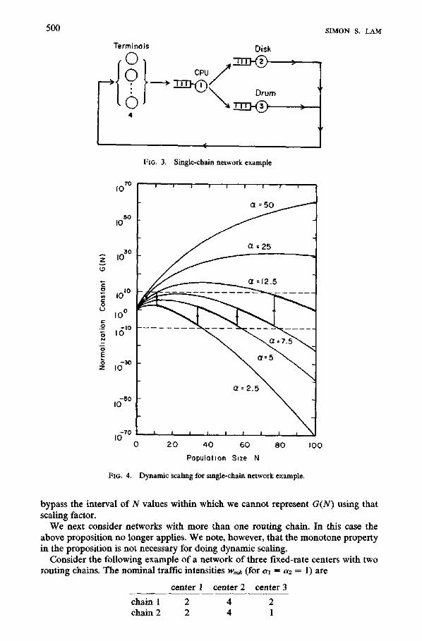
scaling technique, we use an example considered by Chandy and Sauer in [5] and illustrated in Figure 3. Center 4 is an IS center that models a population o f terminals. Centers 1-3 are all fixed-rate centers. The relative arrival rates )~,~ (at a -- 1) and mean service times Tm are as follows:

m )km Tm

1 1 0.020 2 0.2 0.044 3 0.8 0.008 4 0.2 15

In Figure 4, G(N) is shown as a function of N for different values of a. Suppose we need to compute G(100) on a computer that can only represent floating numbers between l0 -1° to l01°. A dynamic scaling approach then is to start with an arbitrary scaling factor, say a = 50, as shown in Figure 4. When a floating-point overflow is about to occur, a is changed to a smaller value using eq. (l 1). When a floating-point underflow is about to occur, a is changed to a larger value. As shown in Figure 4, after several changes in a we finally found G(100) = 0.1430 for a = 12.5 without exceeding the 10-1°10 ~° floating-point range. It was not unlikely that we ended up with a scaling factor that we used earlier, but the scaling technique enabled us to

500

0

0

e -

.9 N

E

z

Terminals

4

Disk

cPO/t

i 0 7°

5o IO

i0 3°

i0 a°

i 0 °

i(~ IO

io -3o

- 5 O IO

-7O I0

FIG. 4.

(

FIG. 3. Single-chain network example

a =50

a = 2 5

=12.5

a = 5

(Z -- 2.5

f

0 2 0 4 0 60 80

Population S=ze N

Dynamic scaling for single-chain network example.

I 0 0

SIMON S. LAM

bypass the interval of N values within which we cannot represent G(N) using that scaling factor.

We next consider networks with more than one routing chain. In this case the above proposition no longer applies. We note, however, that the monotone property in the proposition is not necessary for doing dynamic scaling.

Consider the following example o f a network o f three fixed-rate centers with two routing chains. The nominal traffic intensities w,~ (for al = a2 = 1) are

center 1 center 2 center 3

chain 1 2 4 2 chain 2 2 4 1

Queuing Network Normalization Constants

TABLE I. NORMALIZATION CONSTANTS AND THEIR SCALING FACTORS FOR THE Two-CHAIN NETWORK EXAMPLE

501

(N~, N2)

(0, 0) (0, 1) (1, 0) (1, 1) (0, 2) (2, 0) (1, 2) (2, 1) (2, 2) m = 1 G 1 2 2 8 4 4 24 24 64

ot (1, 1) (1, 1) (1, 1) (1, 1) (1, 1) (1, 1) (1, 1) (1, 1) (1, 1)

G ! 6 6 56 28 28 30 20 30-40

( ~ ) ( ! 1 ) ( 1 1) a O,t) (t,t) (t , l) (t,t) O,t) (t,t) ½,1 ~"~ ~"~

G l 7 8 78 35 44 211 ~ 411- ~

vt ( l , l ) ( l , l ) (1, , , ( , ,1) (1,1) ( l , l ) ( 1 ) ( l ~ ) ( 1 , . ~ )

m=2

m = 3

Let us employ the convolution algorithm for fixed-rate servers from [14]. Let G(a, m, N) denote the normalization constant for the first m centers with scaling factors a and population vector N. We have

K G(a, m, N) = G(a, m - 1, N) + Y, G(a, m, N - lk)pmk for m --> 2,

k=l and

G(a, I, N) = m! Il • k--1 him

The above recursive equation can be rewritten as

G(a, m, N) = r(vt, fl, N)G(fl, m - 1, N) K

+ ~ r(a, ~,, N - l , )G(y, m, N - l~)akwmk, (19) 4--1

where r(a, fl, N) was defined earlier. Suppose in the two-chain network example we want the normalization constant for N = (2, 2). However, the largest value of the normalization constant that we can store is 100. By dynamically changing the scaling factors and employing eq. (19) we arrived at the results tabulated in Table I.

COMPUTATION OF PERFORMANC~ MF.ASURES. As illustrated in the above example, when the normalization constants of more than one population vector are used in the same formula, they need to have the same scaling factors.

Service-center throughput rates can be computed using the formula

Trek(N) ffi ~-,k G(a, M, N - lk) r(a, fl, N)GQS, M, N) ' (20)

where it is assumed that ~lk ~ O~k. The mean queue size qmk(N) for a fixed-rate service center can be computed using the formula

Gm+(a, M, N - lk) qmh(N) = akw,~h r(a, fl, N)G(fl, M, N) ' (21)

where Gm+ is the output of the convolution algorithm over centers 1 - M but with center m convolved twice [14]. In both cases, since the normalization constants needed range over population vectors that differ by one customer, finding a set of scaling factors to fit the normalization constants within a given floating-point range should not pose much of a problem.

502 SIMON S. LAM

A difficulty may arise in the calculation of the mean queue length for a service center for which #,,,(i) is not a constant. In this case the marginal queue-length distribution may need to be first computed as follows:

P,~(n,,)) --p,,,(nm)Gm-(a, M, N -nm) r((~, fl, N)a(fl, M, N) ' (22)

where p,n(n.,) was defined earlier. Gin- is the output of the convolution algorithm over centers 1 - M but skipping over center m. Since nm may range from 0 to N, it will then be likely that we cannot fit the normalization constants of N - nm and N within a given floating-point range using the same scaling factors. However, we observe that if the floating-point range is of reasonable size, then the mean queue length can still be computed accurately by simply discarding those marginal queue- length probabilities Pm(n.,) that are too small and will cause underflows! Let SMALLEST (LARGEST) denote the smallest (largest) floating-point number available. The error introduced in the mean queue length is negligible if

(~-'1 n)SMALLEST << LARGEST for any k.

The above will hold given any nontrivial floating-point range and reasonable chain population sizes.

SPACE OVERI-IEAD CONSIDERATIONS. The additional space overhead of dynamic scaling depends upon the computational algorithm and its implementation. In a convolution algorithm the recursion is done over the service centers. Consequently, an entire array of normalization constants for all population vectors between 0 and N is needed. A straightforward way to provide a mapping between population vectors and their corresponding scaling factors is to provide an entire array of a values. However, an inspection of the example in Table I suggests that since changes occur infrequently, it is possible to provide the mapping between population vectors and scaling factors with substantially less memory than that of an entire array. In the LBANC algorithm the recursion is done over the population vectors; hence additional saving is possible, since an entire array, indexed from 0 to N, of normalization constants is not needed.

The amount of space overhead of dynamic scaling for any computational algorithm can be reduced significantly with the use of the same scaling factor, say or, for all chains (at the expense of, perhaps, some flexibility). This way, only the mapping between N (-- N1 + N2 + . . . + N r ) and ot needs to be remembered and can be accomplished with a minimal amount of space overhead; specifically, only the values of N at which a scaling change occurs need be remembered. In this case let G(~t, M, N) be the normalization constant that we want to scale down (or up). Scaling can be simply accomplished by updating the pair of values of G and ~t for the given M and N as follows:

where N = Nx + N2 + . . . + N r . Let LARGE and SMALL be floating numbers such that

SMALLEST < SMALL < 1 < LARGE < LARGEST.

Suppose we want to keep G within the range (SMALL, LARGE). When G exceeds LARGE, it can be scaled down to near unity with the choice of

1 fl <-- (LARGE)Ira-


When G drops below SMALL, it can be scaled up to near unity with the choice of

1 fl ~-- (SMALL)I/N.

TIME OVERHEAD CONSIDERATIONS. The additional time overhead of dynamic scaling depends upon its implementation which, in turn, depends upon the computational algorithm and the programming language involved.

The implementation of dynamic scaling is simplest if the programming language has provisions for detecting underflows/overflows and recovering from them. In this case the additional time overhead of dynamic scaling is rather insignificant. Each time the scaling factors are changed, eq. (11) needs to be computed. Assuming that the available floating-point range is not too small and G(N) does not fluctuate greatly as a function of N (owing to fluctuations in #re(i)), the frequency of encountering overflow or underflow conditions requiring a change in scaling factors should be very low.

If overflows/underflows cannot be easily detected and recovered from, then it is necessary to prevent their occurrence by testing the magnitude of operands before operations. Upper and lower bounds, LARGE and SMALL, respectively, are needed. Rescaling is required if not all operands lie within these bounds. The basic trade-off in the design of an implementation algorithm is then as follows. In the extreme case, if operands are tested before every arithmetic operation, then the range (SMALL, LARGE) can be chosen to be close to the floating-point range of (SMALLEST, LARGEST). However, given network parameters, bounds may be obtained for SMALL and LARGE so that the testing of operands needs to be performed only once for each group of operations (e.g., subroutine for one convolution, subroutine for mean-queue-length computatmn, etc.).

4. A General Queuing Network Model

The queuing network model described in Section 2 is for closed routing chains, each w~th a fixed number of circulating customers. The model will now be extended to include chains that can have external arrivals and departures. External customer arrival streams to the chains are assumed to be Poisson processes. It is also assumed that a new external arrival to chain k joins class c with probability qc, so that

q c = l . C In R C ( k )

To determine the set of arrival rates (?~mk) for use in the traffic intensities (p,,k), the following set of equations should be used (instead of eq. (1)):

va = qd + ~ Vcpca, d in RC(k), (23) c m RC~'k)

k,nk = ~ Vc. (24) c m S C (m) a n d R C ( k )

There can be two types of Poisson arrival processes.

Type I. The arrival rate of chain-k customers is a function of the total network population N, -/k(N), k = 1, 2 . . . . . K. Define

y(N) ---- y,(N) + y2(N) + . - . + yK(N).

Type 2. The arrival rate of chain-k customers is a function of the number of chain-k customers in the network, yk(Nk), k -- 1, 2 , . . . , K.

504 SIMON S. LAM

For networks with K chains, each of which may be open or dosed, Baskett et al. [1] showed that the product-form solution in eq. (7) becomes

a(n) M e(n) -- "---G-" , ,~ pm(n,~), (25)

wherepm(n,,,) was given by eq. (8), G is the normalization constant and is equal to the sum of the unnormalized solution in eq. (25) over all feasible n states, and

I N(n)--I

,~0 y(i) for type-1 arrivals,

a(n) = (26)

/ ~ Nk~-~ ~'k(i) for type-2 arrivals, k~l t~0

where N(u) is the total number of customers and N~(n) is the total number of chain- k customers in the network for network state n. Note that if all chains are closed, a(n) - l by definition. I f at least one chain is open, then the product-form solution given by eqs. (25) and (26) is applicable if for each closed chain, say chain j, ~,~(i) is set equal to zero in y(i) for networks with type-I arrivals or 3,j(i) is set equal to l for all i in eq. (26) for type-2 arrivals.

One way to view a closed network is that it is an open network, but the routing chain population sizes are kept fixed by two mechanisms:

(l) a loss mechanism whereby a new external arrival is discarded and lost forever; (2) a trigger mechanism whereby a departure from the network triggers the instan-

taneous injection of a customer into the same chain as the departed customer (from an infinite supply of customers).

A dosed network is thus equivalent to a network of open chains with the above two mechanisms in place all the time.

The above mechanisms can be invoked or revoked as a function of the population vector N corresponding to the current state of the network. This strategy gives rise to networks with arbitrary sets of feasible population vectors (see Figure 5). Such networks are said to have population size constraints, and it was shown by this author [8] that if V is an irreducible set of feasible population vectors, then a sufficient condition for the product-form solution in eqs. (25) and (26) to remain valid is: For any k, and population vectors N and N + lk in V, the loss mechanism is invoked for a chain-k external arrival in any network state with population vector N if and only if the trigger mechanism is invoked for a chain-k external departure in any network state with population vector N + lk. (In other words, feasible transitions between adjacent feasible population vectors in Figure 5 are paired.)

The class of networks with population size constraints provides a general model that includes networks with closed chains, networks with open chains, and networks with mixed open and closed chains as special cases. The normalization constant G is given by the sum of the unnormalized product-form solution in eq. (25) over all feasible u states for each feasible population vector in the set V.

Let S denote a detailed network state that is Markovian (see [1]),

s = (s1, s2, . . . , s~ , ) ,

where Sm is the state description of service center m. Let A a be the set of all feasible Markovian network states and :T(N) be the set of

feasible Markovian network states with population vector N. Since V is the set of


(a)

~p N

o5

g Q.

0J

.E O t -

0

chain l open chain 2 closed

Chain I Population Size

(b)

,5 g o

o

o r-

0 0

network w=th population stze constraints

Chain I Populatmn Size

FIG 5. Examples of two-chain networks wtth external arrivals and departures

feasible population vectors, we have

6f = O ha(N). N m V

Note that :T(N) is also the set of feasible states of a closed network with population vector N. We explore below the relationship between the normalization constant G(N) of a dosed network and the equilibrium probability of the aggregate state 6a(N) in a general network. We have found that they are also related to equilibrium state probabilities of a birth-death process traversing over the feasible population vectors in V.

It is shown in [ 1] that the equilibrium probability of a Markovian network state has the product form,

P(S) a II*(S) ~ a(N)I-I(S) = G = G

= a(N)l'Ii(Sl)Yl2(S2) . . . I IM(SM) G ' (27)

where N is the population vector of Markovian network state S, Hm(Sm) is defined in [1], and

N - 1

I ,=I-I ° 7(0 for type-I arrivals,

a(N) = , (28)

/ I~ ~v~ 7k(i) for type-2 arrivals. k = l ~=0

5 0 6 S I M O N S, L A M

LOCAL BALANCE AND THE M =* M PROPERTY. Chandy [3] first observed that the product-form solution P(S ) of many queuing networks has a local balance property, that is, it satisfies certain local balance equations in addition to the global balance equations [1, 8]. This observation has proved to be very useful in the discovery and characterization of the class of BCMP networks [1]. (Another treatment of local balance can be found in the work of Chandy et al. [4].)

Muntz [11] found that individual service centers in BCMP networks have the M =* M property, which can be explained and related to the local balance property as follows. Consider class c in service center m (viewed in isolation). Center m has the M ==~ M property if given that the arrival process of customers to class c is a Poisson process, the departure process of customers from class c is also a Poisson process. Let class c be in chain k. Consider network state S in 6f(N). Let S ~+~ be the set of network states in 6P(N + lk) that are the same as network state S but with an extra class-c customer in service center m. Sm is the mth component of S describ- ing service center m. S+~ ~ is the ruth component of network state S +~ in 5e+c; it de- scribes service center m with the extra class-c customer. IIm(S,,) in the product-form solution was found to satisfy the following sufficient condition for the M ~ M property [11]:

+ +e X rlm(Sme)Rm(Sm - . S~) = v~, (29)

where vc was defined in eq. (23), ~L~ is the set of center-m components of network states in 6 e+~, and R,,(S~ c ---) Sin) is the transition rate from S,+, ¢ to Sm corresponding to the departure of the extra class-c customer from center m. Equation (29) can be rewritten as

= II~(s~ )R~(s~ ~ s~), r~(s~)vo E + " + " (30)

where we can interpret

(a) the left-hand side of eq. (30) to be the "flow" out of state Sm due to class-c arrivals, and

(b) the fight-hand side of eq. (30) to be the flow into state S,, due to dass-c departures.

Equation (30) is an example of a local balance equation. Since it is with respect to the arrivals and departures of a specific class, it will be referred to as a class local balance equation [1, 3].

Since II(S) has a product form, the previous equation can be rewritten as

II(S)vo = E II(S+C)R~(S~ ~ ~ Sin). (31) S + c i n 5 a + e

We next employ eq. (31) to demonstrate a local balance property of H*(S) with respect to external arrivals and departures of a routing chain; this will be referred to as chain local balance. Consider chain k. Suppose the population vectors N and N + lk are in V with transitions between them allowed.

The following identity,

1-- ~ v e i l - ~ p c a l , (32) cmRC(k) dmRC(k) .J

can be easily demonstrated using eq. (23) and ~c,.Rc(k)qc = 1. NOW replace vc in the


fight-hand side of the above using eq. (31) and get

2S+~m..~ c I I ( S )Rm(Sm -'> Sin) 1"~" 2 l-[(S) 1-- ~. p e a .

c in Re(k) dinRC(k)

Let N be the population vector of network state S, and define

f~,k(N) for type-1 arrivals, (33) yk(N) = [ yk(Nk) for type-2 arrivals.

Multiplying both sides of the previous equation by yk(N) and rewriting II(S+~)/II(S) as rI*(S*3/[~h(N)rI*(S)], w e get

II*(S)~'.(N) Z 2 " +° +° [ ] = I I (S )Rm(Sm "'> Sen) 1 - 2 pod , (34) cm RC(k) S+Cm5 a+c din RC(k) .1

which then is a local balance equation satisfied by II*(S) with respect to chain k; note that [ 1 - E d in RC(k)pcd I is the probability that the extra class-c customer departing from center m leaves the network instead of joining another service center. We can interpret

(a) the left-hand side of eq. (34) to be the flow out of state S due to chain-k arrivals, and

(b) the right-hand side of eq. (34) to be the flow into state S due to ehain-k departures.

Note that eq. (34) is applicable only if transitions between N and N + lk are feasible. We have thus shown the following lemma.

LEMMA 3. The class local balance property of rim(Sin) in the product-form solution P( S) implies that P( S) satisfies the chain local balance equation 04).

The chain local balance property of the product-form solution is the key for demonstrating its applicability to the extended class of BCMP networks with population size constraints in [8]. It also has the following immediate consequence.

LEMMA 4 (M =* M PROPERTY FOR A ROUTING CHAIN), I f external arrivals to chain k form a Poisson process with a constant rate Tk, then chain-k customers departing from the network form a Poisson process at the same rate.

The above lemma is easily proved using eq. (34) and Muntz's arguments [11]. Note that any subnetwork of M =* M service centers will have the M =* M property with respect to each chain's external arrivals to the subnetwork and departures from the subnetwork. Hence the subnetwork behaves like a single (composite) M =~ M service center to the rest of the network. (This observation, however, does not apply to networks with the third form of state-dependent service rates if the subnetwork and the set I of service centers overlap partially.)

AGGREGATE STATES AND THEIR OCCUPANCY STATISTICS. Let P(N) denote the equilibriu m probability of the aggregate state 6a(N), defined to be

P(N) = • P(S). SinSa(N)

Let S(t) denote the network state at time t. Consider the case of t ---> oo. We define the conditional throughput rate of chain k as

Tg(N + ID == lira 1 a-~o -A P[S(t) in 6P(N)[ S(t - A) in SP(N + lk)] (35)

5 0 8 S I M O N S. L A M

The next theorem characterizes the occupancy statistics of the aggregate states of a network with population size constraints and relates them to normalization constants of networks which are identical to the given network except that their chains are closed (to be referred to as equivalent closed networks).

THEOREM

(i) The equilibrium aggregate state probabilities are given by

a(N) P(N) -- --G--- G(a, N) for N in V, (36)

where a(N) was defined in eq. (28), G(a, N) is the normalization constant o f an equivalent closed network with population vector N and scaling factors OZk = ?~lk, k = 1, 2 . . . . , K, given by eqs. (23) and (24), and

G = ~,, a(N)G(a, N). (37) N m V

(ii) I f N and N + Is are in V with transitions permitted between them, then the conditional throughput rate is given by

G(a, N) T~(N + Is) - G(~, N + lk)' (38)

and P(N) satisfies the chain local balance equation,

P(N)ys(N) = P(N + Is)T~(N + lk). (39)

PROOF. To show part (i) of the theorem, consider the improper aggregate state probability,

¢r(N) ffi X 1-I*(S) = a(N) Y, II(S). S in..9° (N) S m.9'(N)

Since FI(S) is the (improper) product-form solution of a dosed network [1] with scaling factors ak = Alk, k = 1, 2 . . . . . K, and 6Q(N) is the set of feasible network states with population vector N, we have

~r(N) -- a(N)G(a, N) for N in V.

Normalizing these improper probabilities to sum to one, eqs. (36) and (37) immediately follow.

To show eq. (38) in part (ii) of the theorem, we rewrite eq. (35) as

T~(N + lk) = lim 1 e [ s ( t - A) in 5a(N + ls) and S( t ) in SO(N)]

Taking the limit ~ --> 0 and multiplying both numerator and demoninator by G, we have

T~(N + lk)

= a(N + l~) Y, o m ~ E~m~N~ XS+°m~+° II(s+°)Rm(S+~ °-o Sm)[l -- E ~ m ~ p ~ ]

where

~r(N + lk)

~r(N + lk) = a(N + lk)G(a, N).


Cancel the term a(N + lk) in both the numerator and denominator and note that the expression in the numerator,

E E II(S+~)R~(S +~ --, S~), S m 5,~ (N) S + c m . q "+c

divided by G(a, N + ID, is by definition equal to the throughput rate of class-c customers in an equivalent closed network with population vector N + lk and scaling factors a, which is

v~G(a, N) To(N + lk) --

G(a, N + lk)"

We then have

r t (N + lh) = Tc(N + 1~) [1 - ~ p~d] c m R C ( k ) d m R C ( k )

2 C , ( a , N + l k ) V~ 1 - Y. pod c i n R e ( k ) d m R e ( h i

G(a, N) G(a, N + lk)'

which is eq. (38) in which we have made use of the identity in (32). Equation (39) is a consequence of eqs. (28), (36), and (38). It can also be shown by

summing the chain local balance equation (34) over S in ~(N) and recognizing that the resulting equation is

GP(N)yk(N) * --- GTk (N + 1DP(N + 1D. []

We can interpret eq. (39) as a chain local balance equation satisfied by P(N), since it equates the flow out of the aggregate state ~(N) due to chain-k arrivals to the flows into ~(N) due to chain-k departures.

Let us relate the conditional throughput rate in eq. (38) to previous results. Recall that the throughput rate of a closed network with population vector N + lh is defined to be the throughput rate of service center 1, which is arbitrarily chosen. It is given by

G(a, N) Tk(N + ID ffi ak

G(a, N + 1D'

where ak is equal to the relative arrival rate ?qk of chain-k customers to center 1. The throughput rate of chain-k customers at service center m is given by (~,,~h/~,lh)Tk(N + 10.

Consider chain k which permits external arrivals and departures. Note that h ~ given by eqs. (23) and (24) can be interpreted as the mean number of visits by a chain-k customer to service center m between successive visits to a service center outside the network introduced to act as the source and sink of chain-k customers. For an "open" chain it is physically meaningful to define its throughput rate to be that of its source/sink center. With the set of relative arrival rates defined in eqs. (23) and (24), the relative arrival rate to the source/sink center is unity. Hence

1 Tt (N + Ik) = ~ Tk(N + I D,

which is eq. (38). We make the following additional observations.

510 SIMON S. LAM

FIG. 6l An example of a two-chain network with population size constraints.

N z XI(I)

Tl(2,1

~ T 2 ( 2 , 2 )

0 N I 0 I 2 3

COROLLARY

(0 The equilibrium aggregate state probabilities are the same as the equilibrium state probabilities of a birth-death process with state space V, birth rates ~,(N), and death rates T~ (N + lk) for N and N + 14 in V.

(it) The equilibrium aggregate state probabilities are independent o f f easible transitions in V imposed by the loss and trigger mechanisms.

Part (ii) of the corollary is obvious from Lemma 2. It also implies that P(S) is independent of feasible transitions in V. It does, however, depend upon the set V through the normalization constant G.

AN EXAMPLE. Consider a network with two chains. The set V of feasible population vectors consists o f ( l , 1), (2, 1), (1, 2), and (2, 2). Type-2 arrival processes are assumed. The feasible transitions in V are shown in Figure 6.

Instead of applying eq. (36), we shall solve for P(N~, N2) directly using the local balance eq. (39), from which we get the relationships ~,

Xl(1) 1), P(2, 1) -- T~(2, 1) P(I '

P(2, 2) = A2(I) 1), T2(2, 2) P(2,

~1(1) P(2, 2) = T1(2, 2) P(I ' 2).

Letting P(1, 1) = C and solving for the others in terms of C, we get

P0, I)= C,

P(2, l)= XI(1) 7"1(2, 1) C'

X2(l)~l(1) /'(2, 2) -- 7"2(2, 2)T1(2, 1) C'

7"1(2, 2) A.2(1)A.~(1) P(l , 2) - X~(1) T2(2, 2)T~(2, 1) C"

For sLmplicity we have omitted the * notatton from T~ and T2.


Applying Lemma 2 to the two paths of increasing sequences of population vectors from (1, 1) to (2, 2), we have

/"2(1, 2)/'1(2, 2) = T2(2, 2)Tff2, 1).

We can then rewrite the solution for P(I, 2) as

P(1, 2) - ),2(1) 7"2(1, 2~ C"

The constant C can then be determined from

P(1, 1) + P(2, 1) + P(1, 2) + P(2, 2) -- 1.

E V A L U A T I O N O F T H E N O R M A L I Z A T I O N C O N S T A N T G . The normalization constant G in eq. (37) is evaluated as a summation over the set V o f feasible population vectors. For open chains without population size constraints the set V is infinite. I f the external arrival rates to the open chains are constants, that is,

Tk(N) = yk,

then G can be found easily. First, if all chains in the network are open, then it is well known [ 1 ] that

M 1 G = II , where pm = X pink.

m = l 1 - - pm k

Second, if some of the chains in the network are open while the rest are closed, then it has been shown [14] that

G = Gope, • G(N),

where M 1

Gope.= II 1 po, pO= E pink. m = 1 - - k open

The normalization constant for the closed chains with population vector N can then be evaluated separately with some modifications to account for interactions (if any) between open and closed chains at individual service centers. Let

k closed

(1) At an IS center, open and closed chains do not interact. No modification is necessary in the computation of G(N) with respect to the IS center.

(2) At a fixed-rate center the closed-chain traffic intensity should be modified as follows in the computation of G(N):

p~ P ~ l _ p O ,

to account for the effect of the open chains on the closed chains at this center. (3) At a queue-dependent-service-rate center, the interactions are more complex

than the above, and the effect of the open-chain traffic intensity pO needs to be accounted for by a convolution operation (see [14]).

I f the chain arrival rates "/k(N) depend upon the population vector and /o r the network has population size constraints, then G must be evaluated from eq. (37), repeated here:

G = Y~ a(N)G(a, M, N). N m V

512 SIMON S. LAM

Note that all normalization constants G(a, M, N) of the equivalent closed networks must use the same set of scaling factors, Hence it is likely that no single set of scaling factors can be found so that G(a, M, N), N in V, will fit into a given range of floating- point numbers. Since we are dealing with a summation of terms, if some terms in the sum are too small relative to the others (i.e., underflow occurs), they can be discarded. The error introduced in G is negligible if [ V[ SMALLEST << LARGEST, where I VI denotes the cardinality of V.

5. Conclusions

We have found that previous difficulties with evaluating the normalization constants of closed BCMP queuing networks are due to the use of a fixed set of scaling factors. Normalization constants G(a, M, N) and G(~, M, N) based upon different scaling factors were found to be related very simply by

G(a, M, N) = ak G(~, M, N). k=l

As a result, in the course of evaluating a set of normalization constants (using any computational algorithm) one can repeatedly change the set of scaling factors to avoid overflow or underflow problems that might be encountered. Hence normalization constants for very large population sizes can be obtained with computers having just a modest range of floating-point numbers.

The MVA algorithm of Reiser and Lavenberg [15] bypasses normalization constants and computes various network performance measures directly. It is sometimes desirable to solve a queuing network problem using a hybrid solution method that employs more than one computational algorithm, for example, MVA for fixed-rate servers and convolution for queue-dependent servers. In this case normalization constants are needed and can be computed from the outputs of the MVA algorithm, using eq. (13), for example. Dynamic scaling will then be necessary.

We have also considered BCMP networks with external arrivals, departures, and population size constraints. We have shown that the class local balance property possessed by the product-form solution implies several interesting properties for chains. In particular, external arrivals to a chain and departures from the chain are characterized by the M ~ M property. The relationships between normalization constants of closed networks and equilibrium aggregate state probabilities of networks that permit external arrivals and departures have been examined. We have found that the growth behavior of normalization constants can be modeled by a birth-death process traversing over the set of population vectors.

To show that the results presented in this paper (Lemmas 1-4 and the theorem) are applicable to networks with any or all three forms of state-dependent service rates allowed in BCMP networks, we note that the class local balance equation in eq. (31) is valid for all three forms of state-dependent service rates. Note also that Lemmas 1 and 2 are based on eq. (12), which may be derived from eq. (31). Lemmas 3 and 4 and the theorem are all based on eq. (31).

ACKNOWLEDGMENTS. The author thanks Herbert Schwetman of Purdue University who, as an editor of Communications of the A CM, handled the initial reviewing process of this paper. This paper has benefited from comments on the original manuscript [9] by Peter Denning of Purdue University, and Steve Lavenberg and Charles Sauer of the IBM Thomas J. Watson Research Center. The constructive criticisms of the anonymous referees are also greatly appreciated.

Queuing N e t w o r k N o r m a h z a t i o n Constants 513

REFERENCES

!. BASgETT, F , CnANDY, K.M., MUNTZ, R R, AND PALACIOS, F. Open, closed, and mixed networks of queues with different classes of customers. J ACM 22, 2 (April 1975), 248-260.

2 BUZEN, J.P Computational algorithms for closed queuing networks with exponential servers. Commun ACM 16, 6 (Sept 1973), 527-531

3. CHANDY, K M The analysis and solutions for general queuing networks. Proc 6th Ann Princeton Cord" on Information Sciences and Systems, Prmceton, N.J, 1972, pp. 224-228.

4. CHANDY, K M., HOWARD, J.H, AND TOWSLE¥, D.F. Product form and local balance in queuing networks J ACM 24, 2 (April 1977), 250-263.

5 CO~NOY, KM., AND SAUER, C.H. Computauonal algorithms for product-form queuing networks. Commun. ACM 23, 10 (Oct 1980), 573-583.

6 CHANG, A., AND LAVENBERG, S.S Work rates In closed queuing networks with general independent servers. Oper. Res. 22, 4 (1974), 838-847

7 JACKSON, J.R Jobshop-hke queuing systems Manage Sct 10 (Oct 1963), 131-142. 8. LAM, S.S Queuing networks with population size constraints. IBM J. Res. Devel. 21, 4 (July 1977),

370-378. 9. LAM, S.S Behavior of the normahzatlon constant and a scahng technique for product-form queuemg

networks. Tech. Rep TR-148, Dep of Computer Soences, Umv of Texas, Austin, Texas, June 1980. 10 LAM, S.S., AND LIEr~, Y L. A tree convolution algorithm for the solution ofqueueing networks. Tech.

Rep TR-165, Dep of Computer Sciences, University of Texas, Austin, Texas, Jan. 1981. 11. Mutqxz, R.R Potsson departure process and queuing networks Proc. 7th Ann. Princeton Conf. on

Information Sciences and Systems, Princeton, N.J, March 1973, 435--440 12 MLrNTZ, R.R, AND WONG, J W Asymptotic properties of closed queuing network models. Proc 8th

Ann. Princeton Conf on Informatmn Sciences and Systems, Princeton, N.J., March 1974, 348-352. 13. REISER, M. Numerical methods in separable queuing networks Studies Manage Sci. 7 (1977),

113-142 14. REISER, M., AND KOBaYASHI, H. Queuing networks w,th multiple closed chains: Theory and

computational algorithms IBM J Res. Devel. 19, 3 (May 1975), 283-294. 15 REISER, M, aND LAVENBERG, S.S. Mean-value analysis of closed multichain queuing networks

J ACM 27, 2 (April 1980), 313-322.

RECEIVED JULY 1980, REVISED DECEMBER 1980; ACCEPTED DECEMBER 1980

Journal of the Association for Computing Machine,j. Vol 29. No 2. Ap~i |982

dynamic scaling and growth behavior of queuing … · queuing network normalization constants 493...

Documents