dynamic simulation of a solar powered hybrid sulfur

University of South CarolinaScholar Commons

Theses and Dissertations

2018

Dynamic Simulation of a Solar Powered Hybridsulfur Process for Hydrogen ProductionSatwick BodduUniversity of South Carolina

Follow this and additional works at: https://scholarcommons.sc.edu/etd

Part of the Chemical Engineering Commons

This Open Access Thesis is brought to you by Scholar Commons. It has been accepted for inclusion in Theses and Dissertations by an authorizedadministrator of Scholar Commons. For more information, please contact [email protected].

Recommended CitationBoddu, S.(2018). Dynamic Simulation of a Solar Powered Hybrid sulfur Process for Hydrogen Production. (Master's thesis). Retrievedfrom https://scholarcommons.sc.edu/etd/4820

https://scholarcommons.sc.edu?utm_source=scholarcommons.sc.edu%2Fetd%2F4820&utm_medium=PDF&utm_campaign=PDFCoverPages

https://scholarcommons.sc.edu/etd?utm_source=scholarcommons.sc.edu%2Fetd%2F4820&utm_medium=PDF&utm_campaign=PDFCoverPages

https://scholarcommons.sc.edu/etd?utm_source=scholarcommons.sc.edu%2Fetd%2F4820&utm_medium=PDF&utm_campaign=PDFCoverPages

http://network.bepress.com/hgg/discipline/240?utm_source=scholarcommons.sc.edu%2Fetd%2F4820&utm_medium=PDF&utm_campaign=PDFCoverPages

https://scholarcommons.sc.edu/etd/4820?utm_source=scholarcommons.sc.edu%2Fetd%2F4820&utm_medium=PDF&utm_campaign=PDFCoverPages

mailto:[email protected]

Dynamic Simulation of a Solar Powered Hybrid sulfur Process for

Hydrogen Production

by

Satwick Boddu

Bachelor of Technology,

Indian Institute of Technology - Guwahati, 2014

Submitted in Partial Fulfillment of the Requirements

For the Degree of Master of Science in

Chemical Engineering

College of Engineering and Computing

University of South Carolina

2018

Accepted by:

Edward P. Gatzke, Director of Thesis

Stanford G. Thomas, Reader

John W. Weidner, Reader

Cheryl L. Addy, Vice Provost and Dean of the Graduate School

ii

Abstract

The Hybrid Sulfur process is a thermo-electrochemical cycle used to produce hydrogen

from water. The process requires a high temperature energy source for H2SO4

decomposition with temperature reaching 800°C. This step is followed by SO2 -

depolarized water electrolysis. Using solar energy as the high temperature energy source

allows for efficient environmentally friendly production of hydrogen. This method is an

alternative to traditional photovoltaic electrolysis for hydrogen production. Making the

process economically competitive is a major challenge. Operating the process with

changes in the availability of solar energy also increases process complexity. The

dependence of the process on solar energy requires analysis of the electrolysis and

decomposition sections separately.

The Hybrid Sulphur process was modelled in ASPEN Plus for a target

production rate of 500 gram moles of H2 per second. The process simulation includes

H2SO4 decomposition and O2 separation of the SO2/O2 product from the H2SO4

decomposition. Given the transient nature of solar energy utilized for the decomposition

reaction, analysis of the dynamics of the separation section is of primary importance. A

dynamic simulation was developed with control schemes to stabilize the process. This

simulation was analyzed for step changes in feed flowrate corresponding to the target

hydrogen production rate of 500 gram moles per second. With the proposed controller

iii

configuration, the separation process exhibits time constants ranging from approximately

40 min for a step change in the overall production rate from 100% to 50%. The settling

time for the same production rate change is approximately 60 min. The separation

system can accommodate the system operating a 0% capacity by maintaining column flow

with dilution water. At zero feed the process is functional but it just the recycles the water

from the electrolyzer section through the system making it entirely redundant and

uneconomical. To avoid shutdown of the separation section at low production rates, this

work proposes to include holdup storage tanks for the product streams from the

decomposition section. This will allow the distillation columns to run continuously, but

the separation system must accommodate variable feed rates. Dynamic variation in the

separation section caused by changes in the solar-powered decomposition reactor may

thus be mitigated by use of gas and liquid holdup tanks. The results of these simulation

prove vital in analysis of the viability of the future for large scale hydrogen production

through high temperature Hybrid Sulphur process.

iv

Table of Contents

Abstract ................................................................................................................................ii

List of Figures ....................................................................................................................... v

List of Tables ....................................................................................................................... vi

Chapter 1. Introduction ...................................................................................................... 1

Chapter 2. Chemistry of Hydrogen Production .................................................................. 4

2.1 Hybrid Sulphur Cycle ................................................................................................. 4

2.2 The Bayonet Decomposition Reactor ....................................................................... 7

Chapter 3. Simulation ....................................................................................................... 10

3.1 Steady state simulation ........................................................................................... 10

3.2. Dynamic simulation ................................................................................................ 15

Chapter 4. Results ............................................................................................................. 19

4.1 Steady state results ................................................................................................. 19

4.2 Energy ...................................................................................................................... 19

4.3 Dynamic simulation ................................................................................................. 20

4.4. Analysis of the Dynamic response ......................................................................... 32

4.5. Limitations of the Simulation ................................................................................. 34

Chapter 5. Conclusion ...................................................................................................... 36

Chapter 6. Future Work .................................................................................................... 37

References ........................................................................................................................ 38

Appendix A: Aspen plus results ........................................................................................ 40

v

List of Figures

Figure 2. 1. Schematic diagram of an SO2 – depolarized electrolyzer ................................ 6

Figure 2. 2. Schematic diagram of Bayonet Decomposition Reactor ................................. 9

Figure 3. 1. Schematic diagram of Hybrid Sulphur process (high temperature section) . 12

Figure 3. 2. Hybrid Sulphur process dynamic Simulation ................................................. 13

Figure 3. 3. Gas Separation section .................................................................................. 14

Figure 3. 4. Control schemes in the Aspen Dynamics simulation ..................................... 17

Figure 3. 5. Control schemes in the Aspen Dynamics simulation ..................................... 18

Figure 4. 1. Temperature profile of the decomposition reactor (step change: +25%) .... 21

Figure 4. 2. Sump Liquid level profile in the O2 distillation column (step change: +25%) 22

Figure 4. 3. Pressure profile of the O2 distillation column (step change: +25%).. ............ 23

Figure 4. 4. Liquid level profile of the SO2 distillation column (step change: +25%). ....... 24

Figure 4. 5. Pressure profile of the SO2 distillation column (step change: +25%). ........... 25

Figure 4. 6. Temperature profile of the decomposition reactor (step change: -50%) ..... 26

Figure 4. 7. Sump Liquid level profile in the O2 distillation column (step change: -50%). 27

Figure 4. 8. Pressure profile of the O2 Distillation column (step change: -50%). ............. 28

Figure 4. 9. Sump Liquid level of the SO2 distillation column (step change: -50%). ......... 29

Figure 4. 10. Pressure profile of SO2 distillation column (step change: -50%). ................ 30

Figure 4. 11. Final product stream at zero feed flow rate ................................................ 31

vi

List of Tables

Table 4. 1. Utilities for the steady state SO2 production rate of 1161 Kmol/hr ............... 19

Table 4. 2. Tank sizes for liquid and gas storages for excess decomposition products ... 33

Table 4. 3. Results of control loop response for vital blocks ............................................ 34

Table A. 1 Components specified in Aspen Plus ............................................................... 40

Table A. 2 Global reactions ............................................................................................... 40

Table A. 3 High Temperature reactions ............................................................................ 41

Table A. 4 Decomposition output stream ......................................................................... 42

Table A. 5 Aspen results for the Output stream ............................................................... 44

Table A. 6 Results of Energy analysis on Aspen Plus ........................................................ 45

Table A. 7 The Gaseous stream entering the gas separation section .............................. 46

Table A. 8 The liquid stream entering the separation section ......................................... 48

Table A. 9 Outlet stream after oxygen separation ........................................................... 50

Table A. 10 Design specifications of the Oxygen distillation column ............................... 52

Table A. 11 Design Specifications of the Sulphur Dioxide distillation column ................. 52

Table A. 12 Temperature control on reactors .................................................................. 53

Table A. 13 Sump level control for oxygen separation ..................................................... 53

Table A. 14 Pressure control for oxygen separation ........................................................ 53

Table A. 15 Sump level control for Sulphur dioxide separation ....................................... 54

vii

Table A. 16 Pressure control for Sulphur dioxide separation ........................................... 54

1

Chapter 1. Introduction

The need for renewable and sustainable energy is dictated by the fact of depleting fossil

fuels and an intention to lower the greenhouse gas emissions to fight climate change.

Hydrogen is seen as a means to accomplish this goal in the long term. Hydrogen is an

outstanding storage medium for energy, which is a key component in the Hydrogen

economy. Electricity can be used to produce Hydrogen by splitting water by electrolysis.

Hydrogen is then stored and can be used to generate electricity using efficient fuel cells.

With their heavy dependence on climatic conditions, renewable energies like solar and

wind must address energy storage and transportation problems. Hydrogen is a possible

solution to these problems, paving the way towards a promising future for renewable

energies. Hydrogen is vastly abundant in nature, however not in its pure state. Due to

high reactivity, it is found bound to other elements to form compounds (water,

hydrocarbons). Limited availability of Hydrogen in its basic diatomic form (H2) imposes a

need to find an effective production method.

Hydrogen can be produced from natural gas using high-temperature

steam. This process, called steam methane reforming, accounts for about 95% of the

hydrogen used today in the United States [1]. However this method involves consumption

of fossil fuels and emission of greenhouse gases. Water splitting process are attractive for

hydrogen production due to the abundance of water in the nature and limited emission

2

of greenhouse gases when consumed. Direct electrolysis of water requires electricity

generation. The overall efficiency is of this process likely to be only about 20-24% based

on the Lower heating value (LHV) of hydrogen produced [2]. Processes which promise

efficiencies of over 40% have been identified which use external heat generated by solar

or nuclear sources to power thermochemical water splitting process [2,3,4]. More than

100 processes have been subjected to various analyses and research studies to determine

the potential candidates to produce H2 since 1960’s. Thermochemical cycles using sulfur

often require a high temperature H2SO4 decomposition section. These processes are

among the most attractive options due to their high thermal efficiencies compared to

other competitive processes [5,6,7].

Among the thermochemical cycles examined by the NHI, the Hybrid

Sulphur process and Sulfur-Iodine (SI) process were recognized as effective for nuclear

hydrogen production on large scale [8]. The Sulphur-Iodine cycle is a three step process

with recycling of Iodine and sulphur dioxide. Under International Nuclear Energy Research

Initiative (INERI), the French CEA, General Atomics and Sandia National Laboratories (SNL)

are jointly developing the sulfur-iodine process [9,10,11]. The Hybrid sulphur process

involves a high temperature decomposition step which is followed by electrolysis. The

Hybrid Sulphur cycle has been identified as one of the most advanced processes for solar

hydrogen production, with research activities funded under the DOE-EERE Solar

Thermochemical Hydrogen (STCH) program. SRNL is involved in the STCH project to

determine the feasibility of the Hybrid Sulphur process and developing the components

3

of Hybrid Sulphur process: Bayonet decomposition reactor and SO2 – depolarized

electrolyzer (SDE) [2].

This work focuses on developing a separation section for the sulphuric acid

decomposition products and analyzing the dynamic response for several process

fluctuations (eg. Energy) in decomposition.

4

Chapter 2. Chemistry of Hydrogen Production

2.1 Hybrid Sulphur Cycle:

The Hybrid Sulphur cycle was first proposed by Westinghouse Electric Corporation in

1970s [12,13]. It came to be known as the Westinghouse process after undergoing years

of development. The process involves oxidation and reduction reaction of sulphur. The

entire process involves two major reaction steps: 1] High temperature decomposition of

H2SO4 and 2] SO2 depolarized electrolysis of water.

The decomposition of H2SO4 is endothermic, effectively proceeding with an

external heat supply at temperatures higher than 800 OC. This decomposes sulphuric acid

to produce sulphur trioxide (SO3) and steam (H2O):

H2SO4 --> SO3 + H2O

Sulphur trioxide is dissociated to SO2 and O2 by further catalytic heating.

SO3 -----> SO2 + 1/2O2

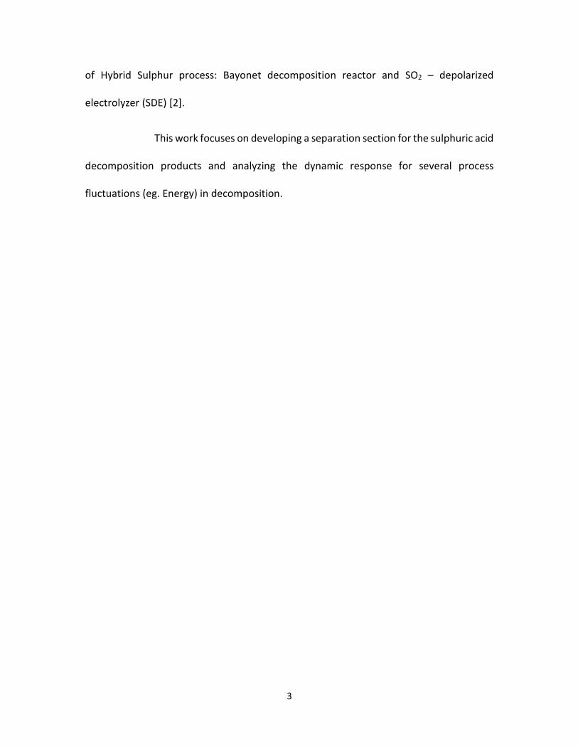
O2 is removed from the decomposition products as a by-product by

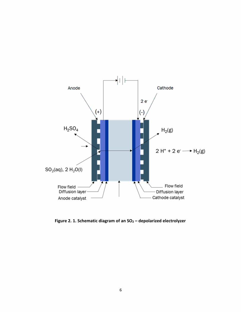
distillation. The remaining mixture of H2O, SO2 and unreacted H2SO4 is fed to the anode

of the sulphur dioxide electrolyzer (SDE). The SO2 in the mixture is electrochemically

oxidized at the anode to form H2SO4, protons and electrons.

5

SO2 + 2H2O -----> H2SO4 +2H+ + 2e-

The H2SO4 is recycled back to the decomposition reactor. The protons are

transported across the membrane to the cathode where it recombines with electrons to

form Hydrogen (H2) [14].

2H+ + 2e- ----> H2

Sulphur – Dioxide Electrolysis (SDE) distinguishes the Hybrid Sulphur process

from other the Sulphur cycles. The process has a standard cell potential -0.158 V at 25 OC.

This is 87% less than that of water electrolysis i.e. -1.229V [15]. This leads to far less

consumption of electricity, making the process more efficient and a primary factor in low

cost hydrogen production [3,4]. In practice, water electrolyzers have higher cell potentials

of -1.7 to -2.0 V for most of the commercially viable current densities due to ohmic losses

and electrode over-potentials. Similarly SDEs operate at a cell potential higher than -

0.243V at practical current densities due to the SO2 dissolved [4]. SRNL research was able

to attain a potential of -0.6V at temperature higher than 100 OC and pressure around 10

bar for a current density of 500 mA/cm2 [4,16]. Thus, SDE appears to be a significant

improvement over traditional water electrolysis.

6

Figure 2. 1. Schematic diagram of an SO2 – depolarized electrolyzer

7

2.2 The Bayonet Decomposition Reactor:

A bayonet reactor is preferred to carry out the high temperature sulphuric acid

decomposition. During the NHI, SNL identified the bayonet reactor as the fundamental

design to vaporize and decompose the H2SO4 inside a single component [17]. The reactor

is modelled to be a plug-flow reactor with the feed and heating fluid flowing though

concentric paths. The concentrated H2SO4 feed mixture enters the reactor at 120 0C. It is

vaporized and superheated to around 1075 0C where it decomposes into SO3. Sulphur

trioxide is catalytically decomposed into SO2 and O2. This gaseous mixture is cooled to 480

0C with SO3 re-associating with water to form H2SO4 and further cooled down to 250 0C.

Due to the high-temperature operating conditions of the reactor it is a

challenge to find an appropriate material that can resist these extreme conditions without

corrosion or deterioration. Additionally, the material should have good heat transfer

characteristics. Silicon Carbide (SiC) is proposed as a solution to these problems. SiC can

be used as the tube material for both the external end and internal open closed tubes

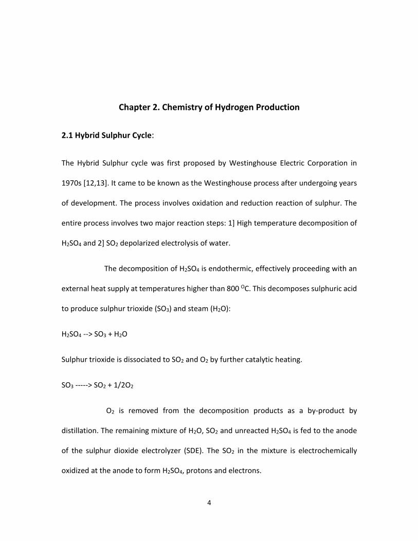
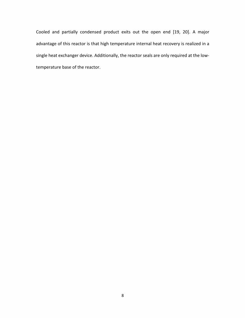
[18]. As depicted in the Figure 2, the reactor consists of one closed ended SiC tube and an

open ended SiC tube both co-axially aligned to form two concentric flow paths. A baffle

tube may be included to enhance heat transfer. Concentrated liquid H2SO4 is fed at the

open end to the annulus, where it is vaporized before passing through an annular catalyst

bed. The decomposition reaction takes place in the catalyst bed, using heat provided by

the external heat source. The products are SO2, O2, and H2O in vapor form. These products

return through the central tube and exchange heat with the feed through recuperation.

8

Cooled and partially condensed product exits out the open end [19, 20]. A major

advantage of this reactor is that high temperature internal heat recovery is realized in a

single heat exchanger device. Additionally, the reactor seals are only required at the low-

temperature base of the reactor.

9

Figure 2. 2. Schematic diagram of Bayonet Decomposition Reactor

High

Temperature

Heat

Outlet: SO2,

O2, H

2O

10

Chapter 3. Simulation

A model of high temperature section of Hybrid Sulphur process with the gas separation

section and decomposition reactor is simulated on ASPEN plus. Given the complexity of

designing a bayonet reactor, a generic stoichiometric reactor was setup with fixed

conversion rates. The output stream from the reactors is passed into the separations

section where distillation is employed. The steady state and dynamic responses of the gas

separations are primarily analyzed for variations in the feed flow rate.

3.1 Steady state simulation:

The Hybrid Sulphur simulation model built with ASPEN plus does not include the

electrolysis process and is limited to decomposition section of the process. The

decomposition section of the process is solar driven, which leads to variations in energy

supply for the decomposition. This unpredictability in the high temperature section

recommends a storage for SO2 produced so that it can be used to run the electrolysis

uninterrupted. Being dynamically different the electrolysis section and high temperature

decomposition section are designed and analyzed separately. Therefore this simulation is

limited only to the decomposition section. The model

11

consists of mainly two sections: 1) High temperature decomposition and 2) separation of

gases.

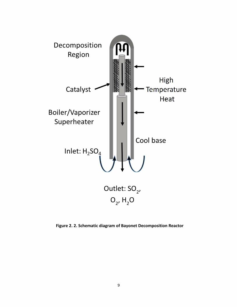
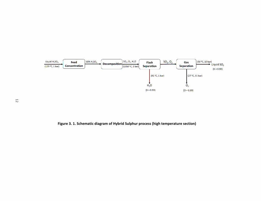
The feed stream to the reactor contains H2SO4 at a concentration of 50

wt% at 120 0C and 1 bar. This feed is decomposed to Sulphur dioxide and oxygen by the

decomposition section. A separator at 145 0C concentrates the sulphuric acid and is then

passed through the decomposition section which is designed with two reactors and a

heater to resemble the original bayonet reactor. The first reactor decomposes the

sulphuric acid at 950 0C at 1 bar to SO3. The second reactor at 950 0C further decomposes

SO3 to SO2 and O2. The material stream from the decomposition reactors are subjected

to further cooling and passed into flash drums to separate liquid and gaseous

components.

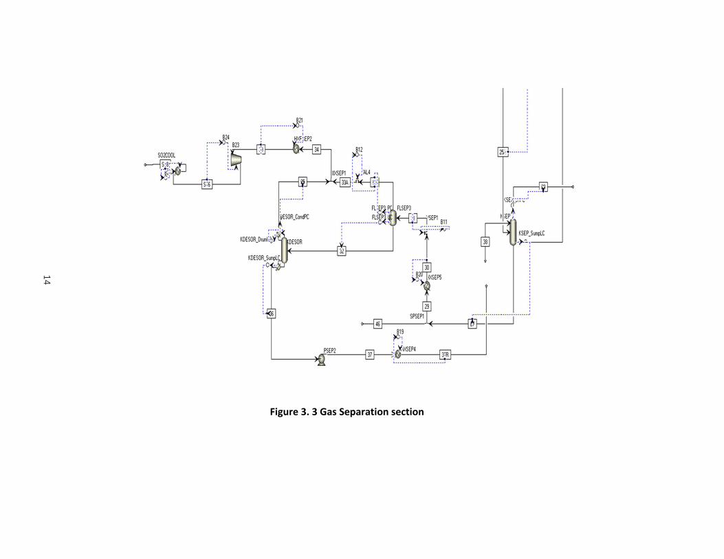
The gas and liquid streams from the high temperature decomposition

section are passed into a separation section. The separation of gases was accomplished

primarily through two distillation columns. The feed to the first distillation column

(number of stages = 15, diameter = 2.21 m, height = 9.144 m) is composed of the gas and

liquid streams from the decomposition section. This column separates the oxygen, leaving

Sulphur dioxide along with water. Sulphur dioxide is completely separated from the water

in the second distillation column (number of stages = 15, reflux ratio = 4, diameter = 4.92

m, height = 7.24 m). After separation, the SO2 may be stored or passed into the

electrolyzer section.

12

Figure 3. 1. Schematic diagram of Hybrid Sulphur process (high temperature section)

13

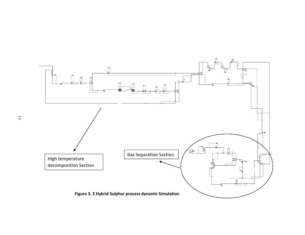
Gas Separation Section High temperature

decomposition Section

Figure 3. 2 Hybrid Sulphur process dynamic Simulation

14

Figure 3. 3 Gas Separation section

15

3.2. Dynamic simulation:

The steady state simulation in Aspen plus is converted to Aspen Dynamics. The model

must have controllers added to maintain stable operation. This allows the process to be

analyzed under various production rates. Controllers are established over various blocks

in the simulation and tuned to enable the system to vary the production rate of sulphur

dioxide upto 50%. The prominent control schemes used for the blocks are:

1) Heaters with specified vapor fraction: Ratio control of input and output volumetric

flow with heat duty as the manipulated variable.

2) Heaters with specified outlet temperature: Feedback reverse acting control with

heat duty as manipulated variable.

3) Tanks: Feedback control with outlet flow as manipulated variable.

4) Reactors: Feedback control of reactor temperature with heat duty being the

manipulated variable.

5) Flash separators: Feedback control of pressure and liquid level of the blocks by

controlling the flow rate of gas and liquid streams respectively.

6) Distillation Columns: Sump level control by bottom stream flowrate and pressure

control by overhead stream flowrate.

16

The controllers on the distillation columns and other blocks are tuned to

proper parameters for efficient transition between different production rates. The

settling time for distillation columns post the step change were upto 2-3 hours for the

above mentioned transitioned. The controllers needed large Gain to make the process

rapid and smooth. Such large gains however raise serious stability issues and complexities

in practical applications.

17

Property controlled : Liquid level Controlled : Liquid level and pressure

Set-point : 6.19 m Set-point : 2.83 m and 11.4 bar

Figure 3. 4. Control schemes in the Aspen Dynamics simulation

18

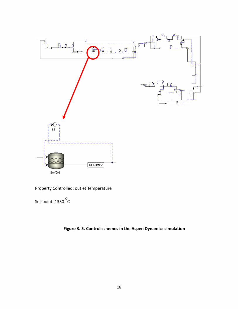
Property Controlled: outlet Temperature

Set-point: 1350 O

C

Figure 3. 5. Control schemes in the Aspen Dynamics simulation

19

Chapter 4. Results

The simulation is run on ASPEN Plus which analyzes the system under steady state. The

simulation is then converted to ASPEN dynamics and results were recorded for the

changes in feed flowrates.

4.1 Steady state results:

A feed stream of H2SO4 (50% wt) enters the system at a rate of 11,606 Kmol/hr at 120 OC.

After carrying out both the high temperature decomposition and gas separations the

simulation model managed to generate 1161 Kmol/hr of Sulphur dioxide which is

stored/passed into the electrolysis section. Oxygen gas of 894 Kmol/hr is produced as a

by-product.

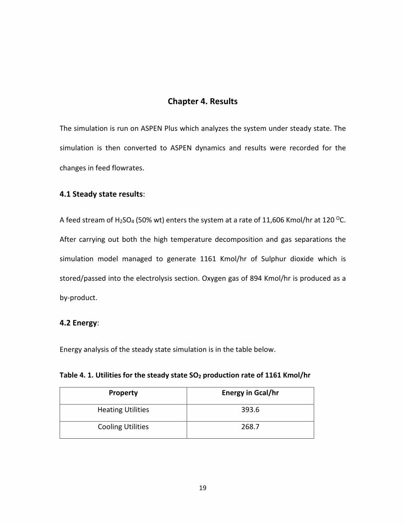
4.2 Energy:

Energy analysis of the steady state simulation is in the table below.

Table 4. 1. Utilities for the steady state SO2 production rate of 1161 Kmol/hr

Property Energy in Gcal/hr

Heating Utilities 393.6

Cooling Utilities 268.7

20

4.3 Dynamic simulation:

The dynamic simulation is subjected to changes in the input feed flowrate. The controllers

placed on each block is tuned enough to make the transitions quick and effective. The

simulation is analyzed for an increase to 14606 Kmol/hr and decrease to 5803 Kmol/hr

from steady state for the input feed flowrate. The dynamic simulation does scale down

much more than 50% but the ASPEN dynamics is ineffective in recognizing the empty

trays. The step down in production rates is limited to 50% to ensure no empty trays. The

dynamics of the decomposition reactor are limited to the temperature. A better design

of the reactor would have enabled us to analyze the transience of the decomposition

reaction.

Dynamic response for the feed flow rate changes of some blocks are depicted

below. There was no oscillatory or inverse responses observed.

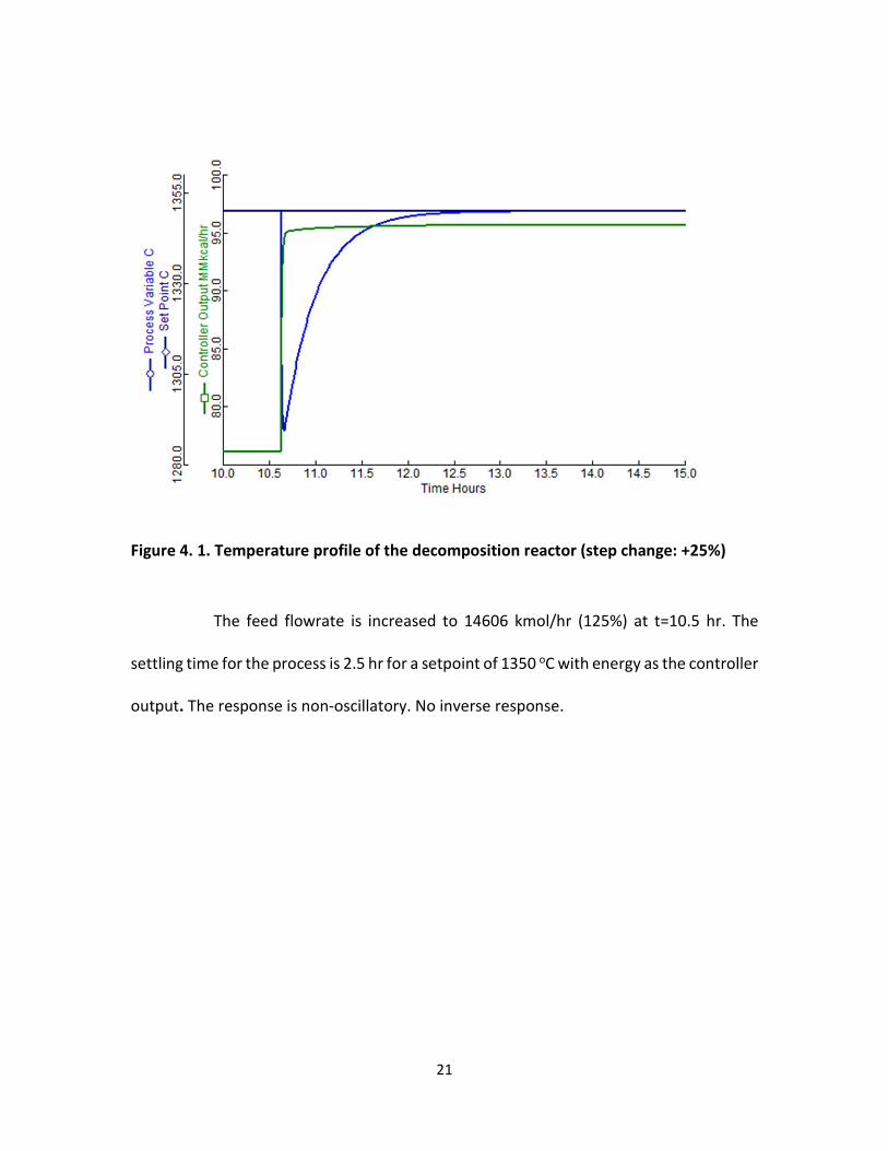
4.3.1 For an increase of 25% in feed flowrate:

The amount of SO2 now produced is 1149 kmol/hr with traces of oxygen and 118 kmol/hr

of water in the output stream. The feed flowrate is increased to 14606 kmol/hr (125%) at

t=10.5 hr. The system settles back to the steady state in about 2 hrs.

21

Figure 4. 1. Temperature profile of the decomposition reactor (step change: +25%)

The feed flowrate is increased to 14606 kmol/hr (125%) at t=10.5 hr. The

settling time for the process is 2.5 hr for a setpoint of 1350 oC with energy as the controller

output. The response is non-oscillatory. No inverse response.

22

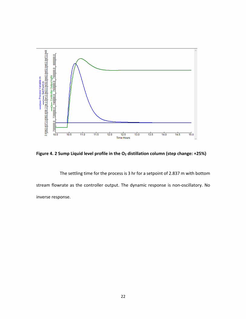
Figure 4. 2 Sump Liquid level profile in the O2 distillation column (step change: +25%)

The settling time for the process is 3 hr for a setpoint of 2.837 m with bottom

stream flowrate as the controller output. The dynamic response is non-oscillatory. No

inverse response.

23

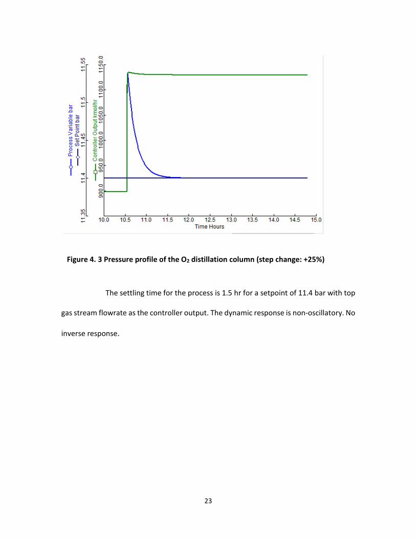
Figure 4. 3 Pressure profile of the O2 distillation column (step change: +25%)

The settling time for the process is 1.5 hr for a setpoint of 11.4 bar with top

gas stream flowrate as the controller output. The dynamic response is non-oscillatory. No

inverse response.

24

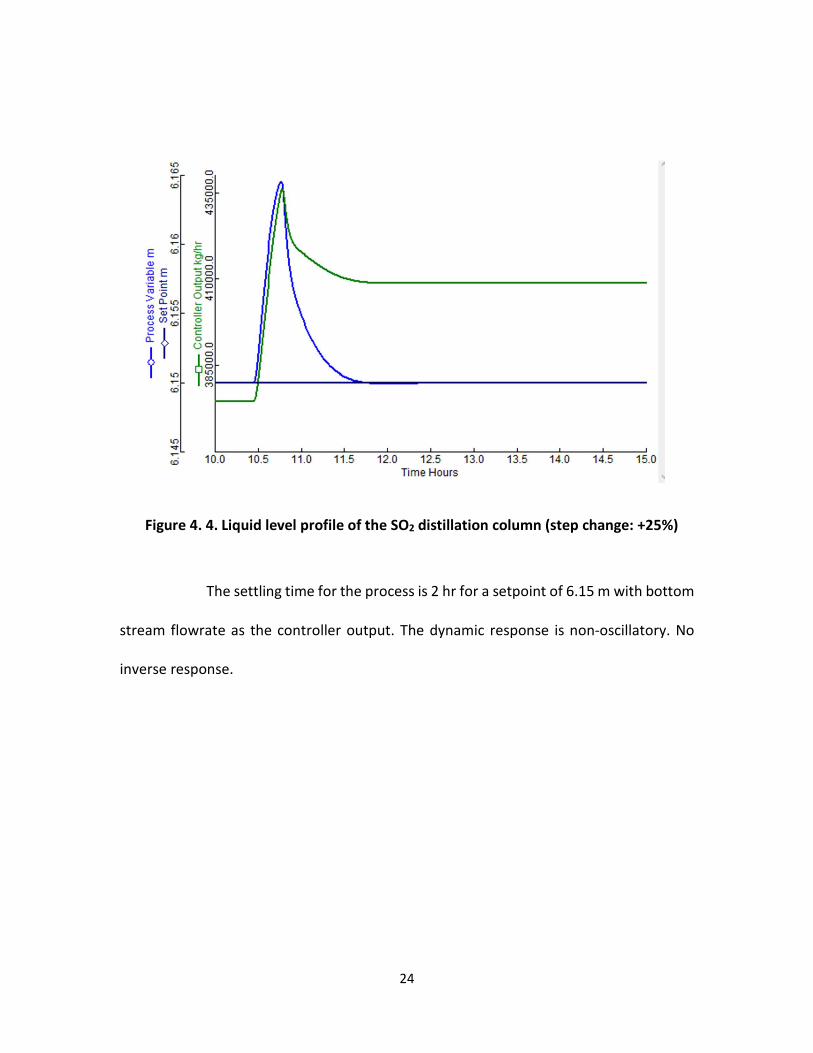
Figure 4. 4. Liquid level profile of the SO2 distillation column (step change: +25%)


stream flowrate as the controller output. The dynamic response is non-oscillatory. No

inverse response.

25

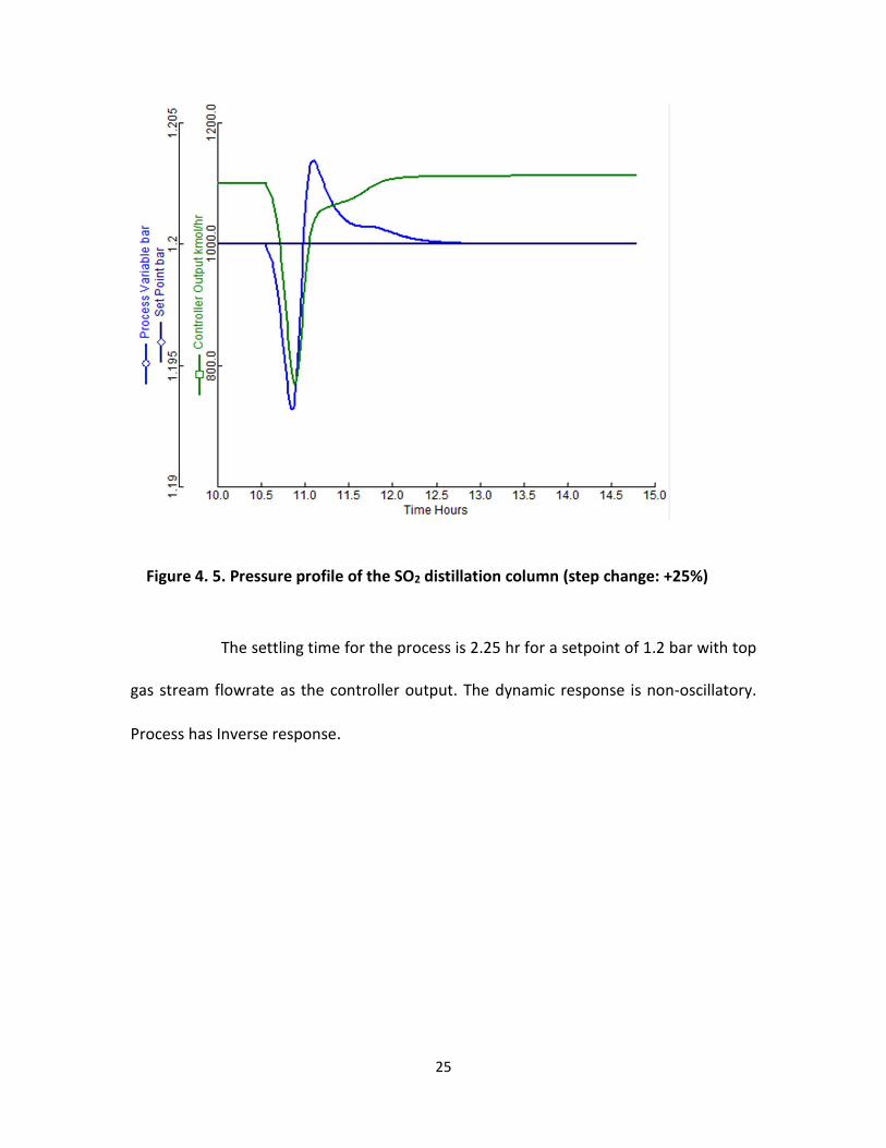
Figure 4. 5. Pressure profile of the SO2 distillation column (step change: +25%)

The settling time for the process is 2.25 hr for a setpoint of 1.2 bar with top

gas stream flowrate as the controller output. The dynamic response is non-oscillatory.

Process has Inverse response.

26

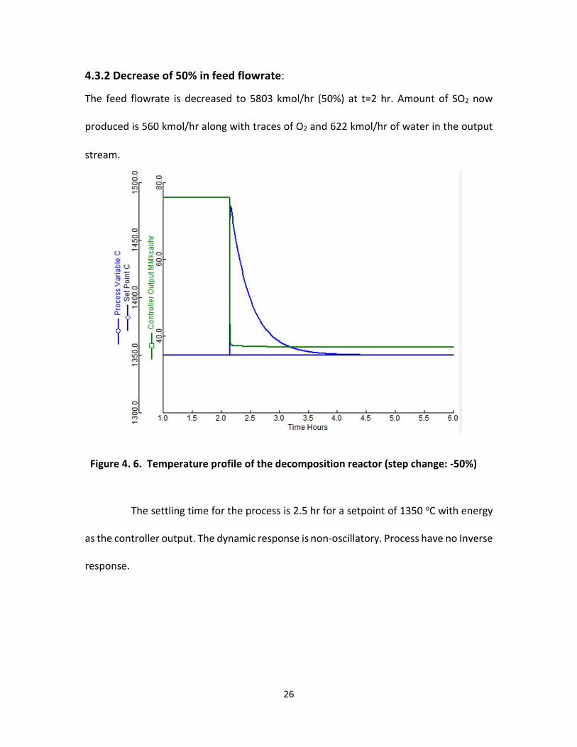
4.3.2 Decrease of 50% in feed flowrate:

The feed flowrate is decreased to 5803 kmol/hr (50%) at t=2 hr. Amount of SO2 now

produced is 560 kmol/hr along with traces of O2 and 622 kmol/hr of water in the output

stream.

Figure 4. 6. Temperature profile of the decomposition reactor (step change: -50%)

The settling time for the process is 2.5 hr for a setpoint of 1350 oC with energy

as the controller output. The dynamic response is non-oscillatory. Process have no Inverse

response.

27

Figure 4. 7. Sump Liquid level profile in the O2 distillation column (step change: -50%)


stream flowrate as the controller output. The dynamic response is non-oscillatory.

Process has no Inverse response.

28

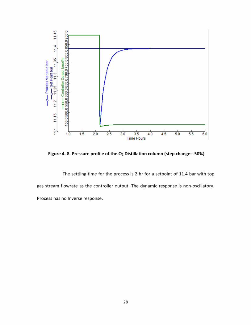
Figure 4. 8. Pressure profile of the O2 Distillation column (step change: -50%)

The settling time for the process is 2 hr for a setpoint of 11.4 bar with top

gas stream flowrate as the controller output. The dynamic response is non-oscillatory.


29

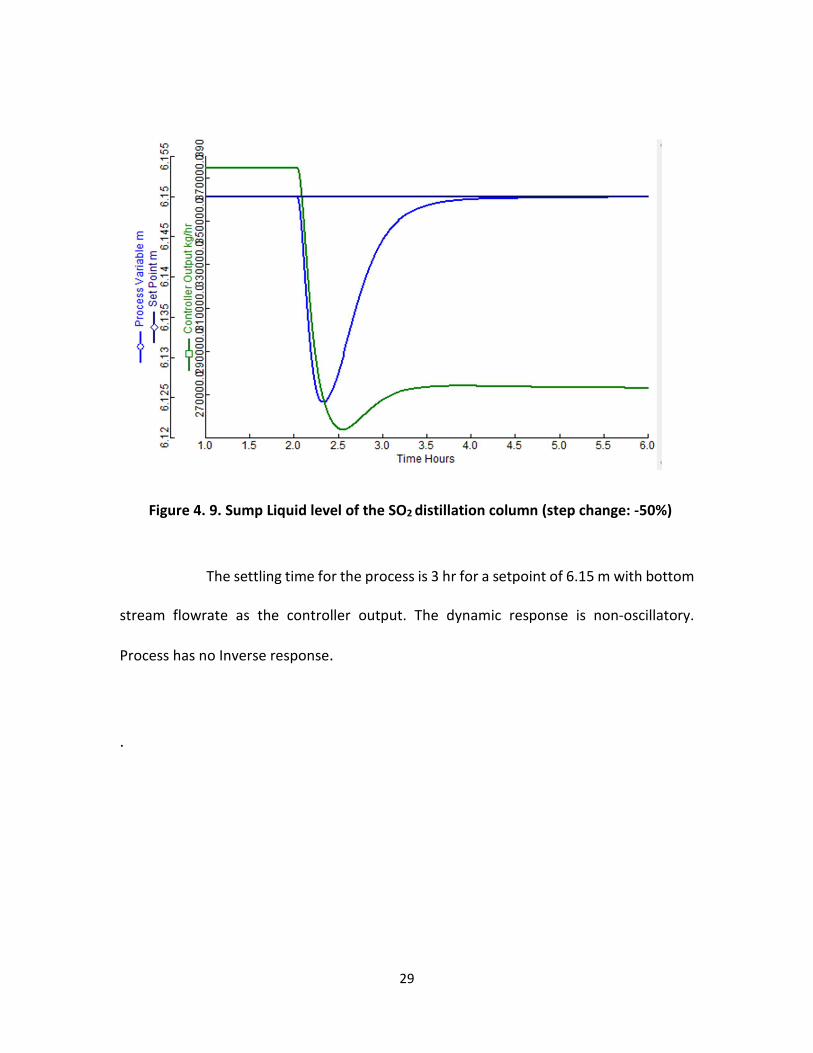
Figure 4. 9. Sump Liquid level of the SO2 distillation column (step change: -50%)


stream flowrate as the controller output. The dynamic response is non-oscillatory.


.

30

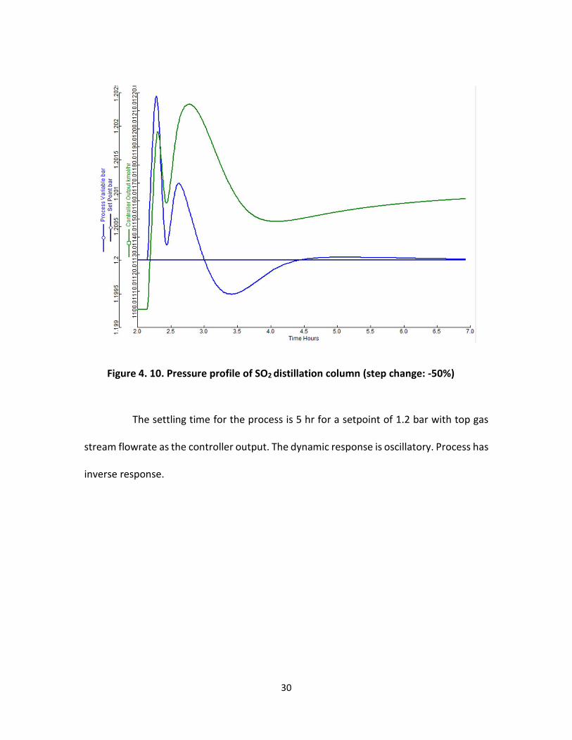
Figure 4. 10. Pressure profile of SO2 distillation column (step change: -50%)

The settling time for the process is 5 hr for a setpoint of 1.2 bar with top gas

stream flowrate as the controller output. The dynamic response is oscillatory. Process has

inverse response.

31

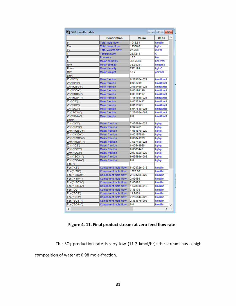
Figure 4. 11. Final product stream at zero feed flow rate

The SO2 production rate is very low (11.7 kmol/hr); the stream has a high

composition of water at 0.98 mole-fraction.

32

4.4. Analysis of the Dynamic response

The important components of the simulation like distillation columns are stable for major

step changes in the feed. The controller action is swift and had a settling time of around

2-3 hours for the vital blocks of the simulation (Figure 4.7, Figure 4.9). The average time

constant of the process is estimated to be 40 min (table 4.3). The controllers are set to

large gains in the order of 30 to attain a faster transient response. The simulation cannot

handle feed flowrates more than 14606 kmol/hr, which is 25% higher than the steady

state value. The production rates at 25% above the steady state value are rarely achieved

due to the nature of solar energy. The 25% scale up is adequate. The decomposition

process is subjected to rapid changes in energy input. The step changes in the feed above

8000 kmol/hr resulted in severe errors in the thermodynamic property package ENRTL –

RK.

Though the process does not scale down to zero directly for a single step

change, the simulation does not break down at zero feed flow rate. The recycled water

stream from the electrolyzer fuels the system in the case of zero feed flow and the system

is just processing the water (Figure 4.11). This makes running the process at zero flow rate

completely redundant. Shutdown of the separation system at lower production rates is

an efficient option. A high level energy/economic optimization is needed to decide the

flowrates below which it is inefficient to run the separation system. Storage tanks can be

used to collect excess liquid and gaseous streams out of the decomposition section while

the decomposition section is processing at higher production rates (100-125%). This gas

33

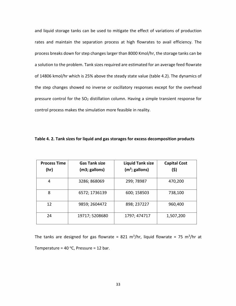
and liquid storage tanks can be used to mitigate the effect of variations of production

rates and maintain the separation process at high flowrates to avail efficiency. The

process breaks down for step changes larger than 8000 Kmol/hr, the storage tanks can be

a solution to the problem. Tank sizes required are estimated for an average feed flowrate

of 14806 kmol/hr which is 25% above the steady state value (table 4.2). The dynamics of

the step changes showed no inverse or oscillatory responses except for the overhead

pressure control for the SO2 distillation column. Having a simple transient response for

control process makes the simulation more feasible in reality.

Table 4. 2. Tank sizes for liquid and gas storages for excess decomposition products

The tanks are designed for gas flowrate = 821 m3/hr, liquid flowrate = 75 m3/hr at

Temperature = 40 oC, Pressure = 12 bar.

Process Time

(hr)

Gas Tank size

(m3; gallons)

Liquid Tank size

(m3; gallons)

Capital Cost

($)

4 3286; 868069 299; 78987 470,200

8 6572; 1736139 600; 158503 738,100

12 9859; 2604472 898; 237227 960,400

24 19717; 5208680 1797; 474717 1,507,200

34

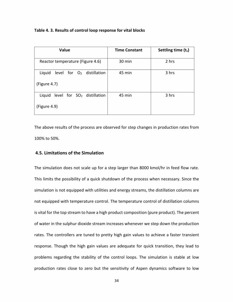
Table 4. 3. Results of control loop response for vital blocks

Value Time Constant Settling time (ts)

Reactor temperature (Figure 4.6) 30 min 2 hrs

Liquid level for O2 distillation

(Figure 4.7)

45 min 3 hrs

Liquid level for SO2 distillation

(Figure 4.9)

45 min 3 hrs

The above results of the process are observed for step changes in production rates from

100% to 50%.

4.5. Limitations of the Simulation

The simulation does not scale up for a step larger than 8000 kmol/hr in feed flow rate.

This limits the possibility of a quick shutdown of the process when necessary. Since the

simulation is not equipped with utilities and energy streams, the distillation columns are

not equipped with temperature control. The temperature control of distillation columns

is vital for the top stream to have a high product composition (pure product). The percent

of water in the sulphur dioxide stream increases whenever we step down the production

rates. The controllers are tuned to pretty high gain values to achieve a faster transient

response. Though the high gain values are adequate for quick transition, they lead to

problems regarding the stability of the control loops. The simulation is stable at low

production rates close to zero but the sensitivity of Aspen dynamics software to low

35

material content in the distillation trays is questionable. The separation section requires

a shutdown at low production rates, the cutoff value for feed flowrate is unknown by the

study. Further energy/economic optimization is required to determine the minimum feed

flowrate required to run the separation process.

36

Chapter 5. Conclusion

Large scale hydrogen production is vital to a future of sustainable energy. The hybrid

Sulphur process is one thermochemical cycle which is recognized as an alternative for

hydrogen production. The Aspen simulation of high temperature section is analyzed for

the steady state and dynamic response of the separation section. The steady state

simulation generates 1161 Kmol/hr of SO2 and 894 Kmol/hr of O2 as a by-product. The

process is mainly solar powered which subjects the process to significant variations in

energy supply in a day. The simulation is now equipped with control loops tuned to

efficient parameters and analyzed dynamically. Maximum step change of 8000 kmol/hr

in the feed flowrate is executed before simulation breakdown. Most of the blocks of the

gas separations were able to re-stabilize back to their steady states within 2 -3 hours on

average for a step change in production rates. The process had a time constant of 20 min.

At low flowrates, shutdown of the separation section and collecting the decomposition

product streams into storage tanks is an efficient option. A rapid and stable dynamic gas

separation section for the hybrid Sulphur process is simulated. Further work in this area

can make hybrid sulphur process a feasible option for large scale hydrogen production.

37

Chapter 6. Future Work

The Hybrid Sulphur process requires further design to fully realize it as a practical option

to produce hydrogen at an industrial scale. The high fidelity model of the reactor is

desired. Building customized models of reactors with use of a software like Aspen custom

modeler can lead to great precision in the design of the reactors. Heaters need to be

replaced by heat exchangers and further improve the energy management by heat

integration. Optimization of the process is required. The dynamic simulation which is now

equipped with basic control schemes like feed-back control with high gain parameters to

ensure a quick transition between production rates. This could lead to stability issues for

the control loops and can lead to difficulties in practical execution. So, advanced control

methods like model predictive control are needed to be employed to ensure better

functioning of the separations section. The response of the separation system is on the

order of 2-3 hours, indicating that transient response may be quite difficult to execute in

reality without some thermal holdup / storage. The separations section of the simulation

does not include removal of unreacted sulphuric acid. Additional process for sulphuric

acid removal before electrolysis is also necessary.

38

References

1. Fuel cell technologies office, Energy efficiency and renewable energy, Department

of Energy, April 2016.

2. Cladio Corgnale, William A. Summers, Solar hydrogen production by Hybrid

Sulphur process, International Journal of Hydrogen Energy 36(2011) 11604-11619

3. Claudio Corgnale, Sirivatch Shimpalee, Maximilian B. Gorensek, Pongsarun

Satjaritanun, John W.Weidner, William A.Summers, Numerical modeling of a

bayonet heat exchanger-based reactor for sulfuric acid decomposition in

thermochemical hydrogen production processes, International journal of

Hydrogen energy, volume 42, issue 32, 10 August 2017, Pages 20463-20472,

4. Maximilian B. Gorensek, William A. Summers. Hybrid sulfur flowsheets using PEM

electrolysis and a bayonet decomposition reactor. International journal of

hydrogen energy 34 (2009) 4097 – 4114.

5. Ginosar DM, Glenn AW, Petkovic LM, Burch KC. Stability of supported platinum

sulfuric acid decomposition catalysts for use in thermochemical water splitting

cycles. Int. J Hydrogen Energy 2007; 32(4):482–8. Brown LC, Besenbruch GE,

Lentsch RD, Schultz KR, Funk JF, Pickard PS, et al. High efficiency generation of

hydrogen fuels using nuclear power. Final Technical Report from General Atomics

Corp. to US DOE. GA-A24285; 2003.

6. Funk JE. Thermochemical hydrogen production: past and present. Int. J Hydrogen

Energy 2001; 26 (3):185e90.

7. L.C. Brown, G.E. Besenbruch, R.D. Lentsch, K.R. Schultz, J.F. Funk, P.S. Pickard, et

al., High efficiency generation of hydrogen fuels using nuclear power, Final

Technical Report from General Atomics Corp. to US DOE. GA-A24285 (2003).

8. M.B. Gorensek, W.A. Summers, C.O. Bolthrunis, E.J. Lahoda, D.T. Allen, R.

Greyvenstein, Hybrid sulfur process reference design and cost analysis, report,

May 12, 2009; South Carolina.

9. Giovanni Cerri, Coriolano Salvini, Claudio Corgnale, Ambra Giovannelli, Daniel De

Lorenzo Manzano, Alfredo Orden Martinez, Alain Le Duigou, Jean-Marc Borgard,

Christine Mansilla, Sulfur–Iodine plant for large scale hydrogen production by

nuclear power, International Journal of Hydrogen Energy, Volume 35, Issue 9, May

2010, Pages 4002-4014.

39

10. S. Goldstein, J.M. Borgard, X. Vitart, Upper bound and best estimate of the

efficiency of the iodine sulphur cycle, Int J Hydrogen Energy, 30 (6) (2005), pp. 619-

626.

11. International Nuclear Energy Research Initiative, 2006 Annual Report. DOE/NE-

131.Washington, DC: United States Department of Energy, 2007. p. 113.

12. Lee E. Brecher and Christopher K. Wu, Electrolytic decomposition of water,

Westinghouse Electric Corp., Patent 3,888,750, June 10, 1975.

13. L.E. Brecher, S. Spewock, C.J. Warde, The Westinghouse Sulfur Cycle for the

thermochemical decomposition of water, Int J Hydrogen Energy, 2 (1) (1977), pp.

7-15.

14. M.B. Gorensek, Hybrid sulfur cycle flowsheets for hydrogen production using high

temperature gas-cooled reactors, Int. J Hydrogen Energy, 36 (20)(2011), pp.

12725-12741.

15. M.B. Gorensek, J.A. Staser, T.G. Stanford, J.W. Weidner, A thermodynamic analysis

of the SO2/H2SO4 system in SO2-depolarized electrolysis, Int. J Hydrogen Energy,

34 (15)(2009), pp. 6089-6095.

16. A.G. Niehoff, N.B. Botero, A. Acharya, D. Thomey, M. Roeb, C. Sattler, R. PitzPaal,

Process modelling and heat management of the solar hybrid sulfur cycle, Int. J

Hydrogen Energy, 40 (2015), pp. 4461-4473.

17. R. Moore, P. Pickard, E. Parma, M. Vernon, F. Gelbard; Integrated boiler,

superheater, and decomposer for sulphuric acid decomposition; Sandia Corp.

(2010), US Patent No. 7645437 B1.

18. Maximilian B. Gorensek, Thomas B. Edwards; Energy Efficiency Limits for a

Recuperative Bayonet Sulfuric Acid Decomposition Reactor for Sulfur Cycle

Thermochemical Hydrogen Production, Ind. Eng. Chem. Res. 2009, 48, 7232–7245.

19. Maximilian B. Gorensek, William A. Summers. Hybrid sulfur flowsheets using PEM

electrolysis and a bayonet decomposition reactor. International journal of

hydrogen energy 34 (2009) 4097 – 4114.

20. E.J. Parma, M.E. Vernon, F. Gelbard, R.C. Moore, H.B.J. Stone, P.S. Pickard,

Modeling the sulfuric acid decomposition section for hydrogen production,

Proceedings of 2007 int. topical meeting on safety and techn. of nucl hydrogen

production, Control and Mgmt, Boston (June 24–28, 2007), pp. 154-160.

40

Appendix A: Aspen plus results

Table A. 1 Components specified in Aspen Plus

Component ID Component name

H2O WATER

H2SO4 SULFURIC-ACID

H2 HYDROGEN

O2 OXYGEN

SO2 SULFUR-DIOXIDE

SO3 SULFUR-TRIOXIDE

H3O+ H3O+

HSO3- HSO3-

HSO4- HSO4-

SO3-- SO3--

SO4-- SO4--

Thermodynamic package: ENRTL-RK

Table A. 2 Global reactions

Reaction Type Stoichiometry

1 Equilibrium H2SO4 + H2O <--> H3O+ + HSO4-

2 Equilibrium H2O + HSO3- <--> H3O+ + SO3--

3 Equilibrium 2 H2O + SO2 <--> H3O+ + HSO3-

4 Equilibrium H2O + HSO4- <--> H3O+ + SO4--

5 Equilibrium SO3 + H2O <--> H2SO4

41

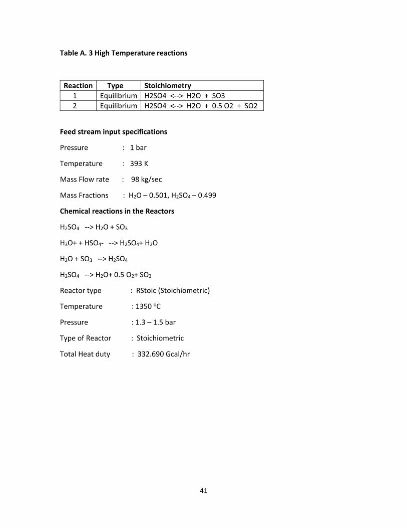
Table A. 3 High Temperature reactions

Reaction Type Stoichiometry

1 Equilibrium H2SO4 <--> H2O + SO3

2 Equilibrium H2SO4 <--> H2O + 0.5 O2 + SO2

Feed stream input specifications

Pressure : 1 bar

Temperature : 393 K

Mass Flow rate : 98 kg/sec

Mass Fractions : H2O – 0.501, H2SO4 – 0.499

Chemical reactions in the Reactors

H2SO4 --> H2O + SO3

H3O+ + HSO4- --> H2SO4+ H2O

H2O + SO3 --> H2SO4

H2SO4 --> H2O+ 0.5 O2+ SO2

Reactor type : RStoic (Stoichiometric)

Temperature : 1350 oC

Pressure : 1.3 – 1.5 bar

Type of Reactor : Stoichiometric

Total Heat duty : 332.690 Gcal/hr

42

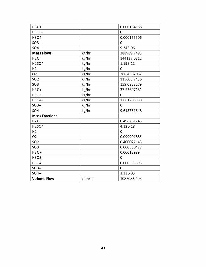
Table A. 4 Decomposition output stream

Description Units DECOMP

Phase

Vapor

Temperature C 1350

Pressure bar 1.33

Molar Vapor Fraction

1

Molar Liquid Fraction

0

Molar Solid Fraction

0

Mass Vapor Fraction

1

Mass Liquid Fraction

0

Mass Solid Fraction

0

Molar Enthalpy kcal/mol -41.80483607

Mass Enthalpy kcal/kg -1549.781454

Molar Entropy cal/mol-K 9.661512004

Mass Entropy cal/gm-K 0.358169856

Molar Density kmol/cum 0.009855128

Mass Density kg/cum 0.265838782

Enthalpy Flow Gcal/hr -447.8709538

Average MW

26.97466535

Mole Flows kmol/hr 10713.37663

H2O kmol/hr 8000.821035

H2SO4 kmol/hr 1.21E-14

H2 kmol/hr 0

O2 kmol/hr 902.2407285

SO2 kmol/hr 1804.481457

SO3 kmol/hr 1.99E+00

H3O+ kmol/hr 1.973275666

HSO3- kmol/hr 0

HSO4- kmol/hr 1.773123859

SO3-- kmol/hr 0

SO4-- kmol/hr 0.100075904

Mole Fractions

H2O

0.746806662

H2SO4

1.13E-18

H2

0

O2

0.08421628

SO2

0.16843256

SO3

0.000185463

43

H3O+

0.000184188

HSO3-

0

HSO4-

0.000165506

SO3--

0

SO4--

9.34E-06

Mass Flows kg/hr 288989.7493

H2O kg/hr 144137.0312

H2SO4 kg/hr 1.19E-12

H2 kg/hr 0

O2 kg/hr 28870.62062

SO2 kg/hr 115603.7436

SO3 kg/hr 159.0823279

H3O+ kg/hr 37.53697181

HSO3- kg/hr 0

HSO4- kg/hr 172.1208388

SO3-- kg/hr 0

SO4-- kg/hr 9.613761648

Mass Fractions

H2O

0.498761743

H2SO4

4.12E-18

H2

0

O2

0.099901885

SO2

0.400027143

SO3

0.000550477

H3O+

0.00012989

HSO3-

0

HSO4-

0.000595595

SO3--

0

SO4--

3.33E-05

Volume Flow cum/hr 1087086.493

44

Table A. 5 Aspen results for the Output stream

Description Units Output stream

Phase

Mixed

Temperature C 29.7

Pressure bar 10


0.00645125


0.99354875


0

Mass Vapor Fraction

0.004962149


9.95E-01

Mass Solid Fraction

0



Molar Entropy cal/mol-K -1.94E+01

Mass Entropy cal/gm-K -0.32407865




Average MW

59.93714435


H2O kmol/hr 111.1810133

H2SO4 kmol/hr 0.00E+00

H2 kmol/hr 0

O2 kmol/hr 4.76E+00

SO2 kmol/hr 1161.473458

SO3 kmol/hr 0

H3O+ kmol/hr 0.012589233

HSO3- kmol/hr 0.012589233

HSO4- kmol/hr 0

SO3-- kmol/hr 4.13E-16

SO4-- kmol/hr 0.00E+00

Mole Fractions

H2O

8.70E-02

H2SO4

0.00E+00

H2

0

O2

3.73E-03

SO2

0.909219532

SO3

0

45

H3O+

9.86E-06

HSO3-

9.86E-06

HSO4-

0

SO3--

3.24E-19

SO4--

0


H2O kg/hr 2002.957084

H2SO4 kg/hr 0.00E+00

H2 kg/hr 0

O2 kg/hr 1.52E+02

SO2 kg/hr 74409.56479

SO3 kg/hr 0

H3O+ kg/hr 0.239480834

HSO3- kg/hr 1.020643024

HSO4- kg/hr 0

SO3-- kg/hr 3.31E-14

SO4-- kg/hr 0.00E+00

Table A. 6 Results of Energy analysis on Aspen Plus

Utilities Actual Target Available

Savings

% of

Actual

Total Utilities

[Gcal/hr]

673.8 374 299.8 44.49

Heating Utilities

[Gcal/hr]

393.6 243.7 149.9 38.08

Cooling Utilities

[Gcal/hr]

280.2 130.3 149.9 53.49

Carbon Emissions

[kg/hr]

0 0 0 0

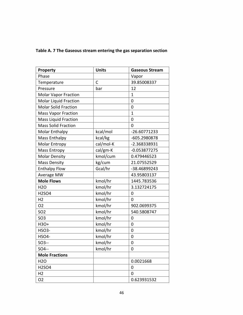
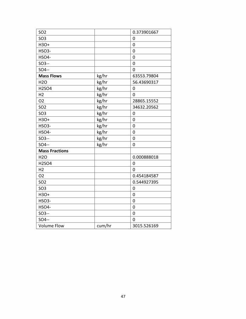
46

Table A. 7 The Gaseous stream entering the gas separation section

Property Units Gaseous Stream

Phase

Vapor

Temperature C 39.85008337

Pressure bar 12


1


0


0

Mass Vapor Fraction

1


0

Mass Solid Fraction

0



Molar Entropy cal/mol-K -2.368338931





Average MW

43.95803137


H2O kmol/hr 3.132724175

H2SO4 kmol/hr 0

H2 kmol/hr 0

O2 kmol/hr 902.0699375

SO2 kmol/hr 540.5808747

SO3 kmol/hr 0

H3O+ kmol/hr 0

HSO3- kmol/hr 0

HSO4- kmol/hr 0

SO3-- kmol/hr 0

SO4-- kmol/hr 0

Mole Fractions

H2O

0.0021668

H2SO4

0

H2

0

O2

0.623931532

47

SO2

0.373901667

SO3

0

H3O+

0

HSO3-

0

HSO4-

0

SO3--

0

SO4--

0


H2O kg/hr 56.43690317

H2SO4 kg/hr 0

H2 kg/hr 0

O2 kg/hr 28865.15552

SO2 kg/hr 34632.20562

SO3 kg/hr 0

H3O+ kg/hr 0

HSO3- kg/hr 0

HSO4- kg/hr 0

SO3-- kg/hr 0

SO4-- kg/hr 0

Mass Fractions

H2O

0.000888018

H2SO4

0

H2

0

O2

0.454184587

SO2

0.544927395

SO3

0

H3O+

0

HSO3-

0

HSO4-

0

SO3--

0

SO4--

0


48

Table A. 8 The liquid stream entering the separation section

Property Units Liquid Stream

Phase

Liquid


Pressure bar 11.76


0


1


0

Mass Vapor Fraction

0


1

Mass Solid Fraction

0








Average MW

22.61748281


H2O kmol/hr 11470.39433


H2 kmol/hr 0

O2 kmol/hr 0.169763076

SO2 kmol/hr 1203.123232

SO3 kmol/hr 1.64E-28

H3O+ kmol/hr 53.248809

HSO3- kmol/hr 53.24823406

HSO4- kmol/hr 0.000536284



Mole Fractions

H2O

0.897513956

H2SO4

1.81E-19

H2

0

O2

1.33E-05

SO2

0.094139736

SO3

1.29E-32

H3O+

0.004166513

49

HSO3-

0.004166468

HSO4-

4.20E-08

SO3--

1.20E-09

SO4--

3.15E-10


H2O kg/hr 206642.3656


H2 kg/hr 0

O2 kg/hr 5.432214713

SO2 kg/hr 77077.84924

SO3 kg/hr 1.32E-26

H3O+ kg/hr 1012.934522

HSO3- kg/hr 4316.977573

HSO4- kg/hr 0.052058249

SO3-- kg/hr 0.001224945

SO4-- kg/hr 0.000386914

Mass Fractions

H2O

0.714887919

H2SO4

7.86E-19

H2

0

O2

1.88E-05

SO2

0.266654048

SO3

4.56E-32

H3O+

0.003504289

HSO3-

0.014934765

HSO4-

1.80E-07

SO3--

4.24E-09

SO4--

1.34E-09


50

Table A. 9 Outlet stream after oxygen separation

Property Units Oxygen stream

Phase

Vapor


Pressure bar 11.4


1


0


0

Mass Vapor Fraction

1


0

Mass Solid Fraction

0




Mass Entropy cal/gm-K -1.51E-01




Average MW

3.20E+01


H2O kmol/hr 3.054659771


H2 kmol/hr 0.00E+00

O2 kmol/hr 8.95E+02



H3O+ kmol/hr 0.00E+00

HSO3- kmol/hr 0

HSO4- kmol/hr 0.00E+00

SO3-- kmol/hr 0

SO4-- kmol/hr 0.00E+00

Mole Fractions

H2O

0.00340189

H2SO4

3.16E-30

H2

0.00E+00

O2

9.97E-01

SO2

9.72E-08

SO3

3.91E-32

H3O+

0.00E+00

HSO3-

0

51

HSO4-

0

SO3--

0

SO4--

0.00E+00


H2O kg/hr 55.03055107


H2 kg/hr 0

O2 kg/hr 28634.93696

SO2 kg/hr 0.005591474

SO3 kg/hr 2.81E-27

H3O+ kg/hr 0.00E+00

HSO3- kg/hr 0

HSO4- kg/hr 0.00E+00

SO3-- kg/hr 0

SO4-- kg/hr 0.00E+00

Mass Fractions

H2O

0.001918111

H2SO4

9.70E-30

H2

0.00E+00

O2

9.98E-01

SO2

1.95E-07

SO3

9.79E-32

H3O+

0

HSO3-

0

HSO4-

0

SO3--

0

SO4--

0


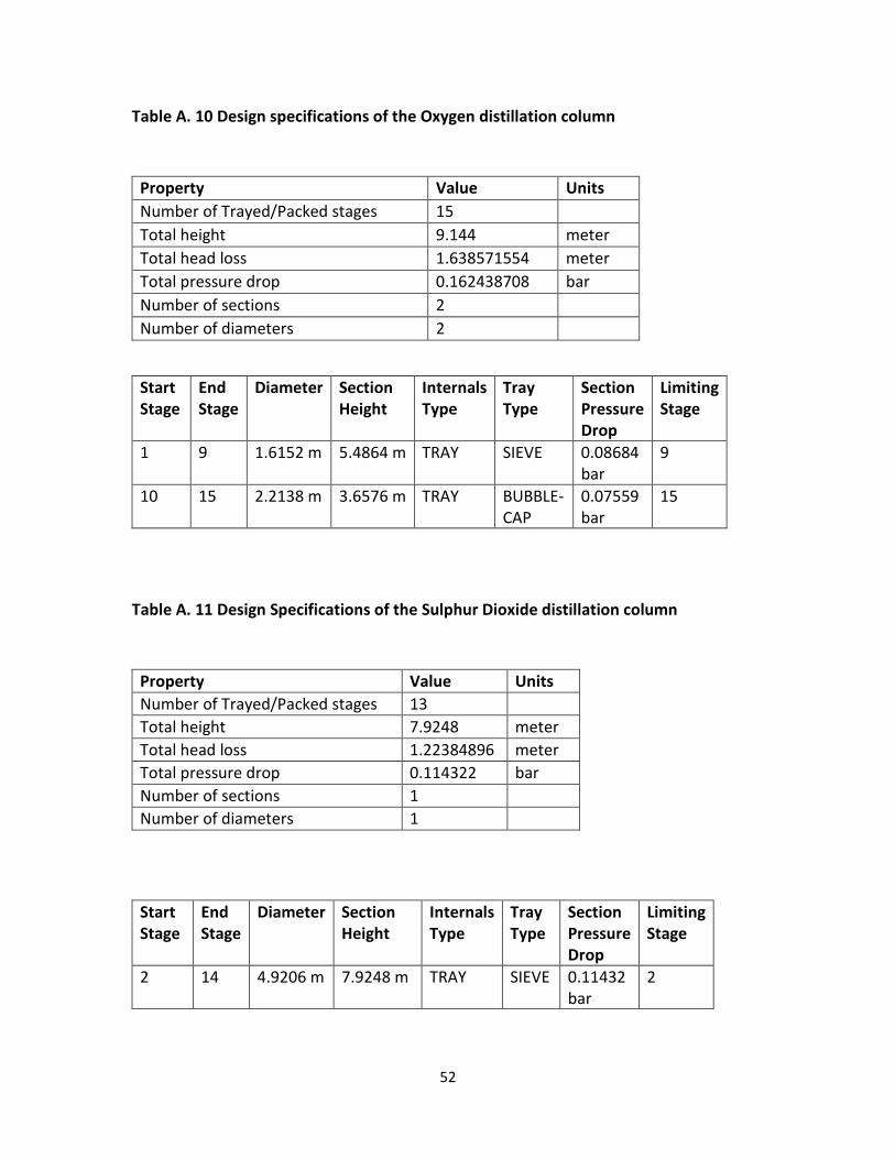
52

Table A. 10 Design specifications of the Oxygen distillation column

Property Value Units

Number of Trayed/Packed stages 15

Total height 9.144 meter

Total head loss 1.638571554 meter

Total pressure drop 0.162438708 bar

Number of sections 2

Number of diameters 2

Start

Stage

End

Stage

Diameter Section

Height

Internals

Type

Tray

Type

Section

Pressure

Drop

Limiting

Stage

1 9 1.6152 m 5.4864 m TRAY SIEVE 0.08684

bar

9

10 15 2.2138 m 3.6576 m TRAY BUBBLE-

CAP

0.07559

bar

15

Table A. 11 Design Specifications of the Sulphur Dioxide distillation column

Property Value Units

Number of Trayed/Packed stages 13

Total height 7.9248 meter

Total head loss 1.22384896 meter

Total pressure drop 0.114322 bar

Number of sections 1

Number of diameters 1

Start

Stage

End

Stage

Diameter Section

Height

Internals

Type

Tray

Type

Section

Pressure

Drop

Limiting

Stage

2 14 4.9206 m 7.9248 m TRAY SIEVE 0.11432

bar

2

53

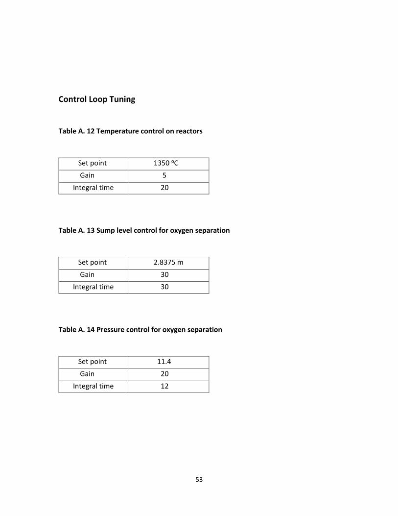
Control Loop Tuning

Table A. 12 Temperature control on reactors

Set point 1350 oC

Gain 5

Integral time 20

Table A. 13 Sump level control for oxygen separation

Set point 2.8375 m

Gain 30

Integral time 30

Table A. 14 Pressure control for oxygen separation

Set point 11.4

Gain 20

Integral time 12

54

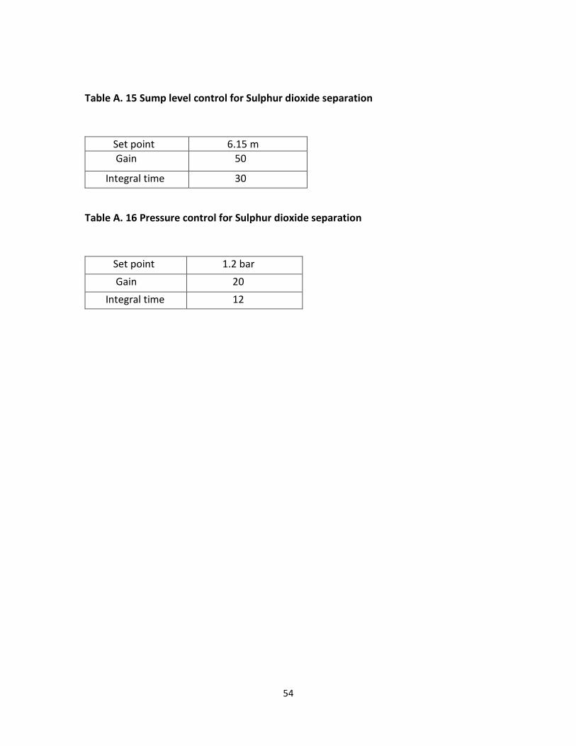
Table A. 15 Sump level control for Sulphur dioxide separation

Set point 6.15 m

Gain 50

Integral time 30

Table A. 16 Pressure control for Sulphur dioxide separation

Set point 1.2 bar

Gain 20

Integral time 12

55

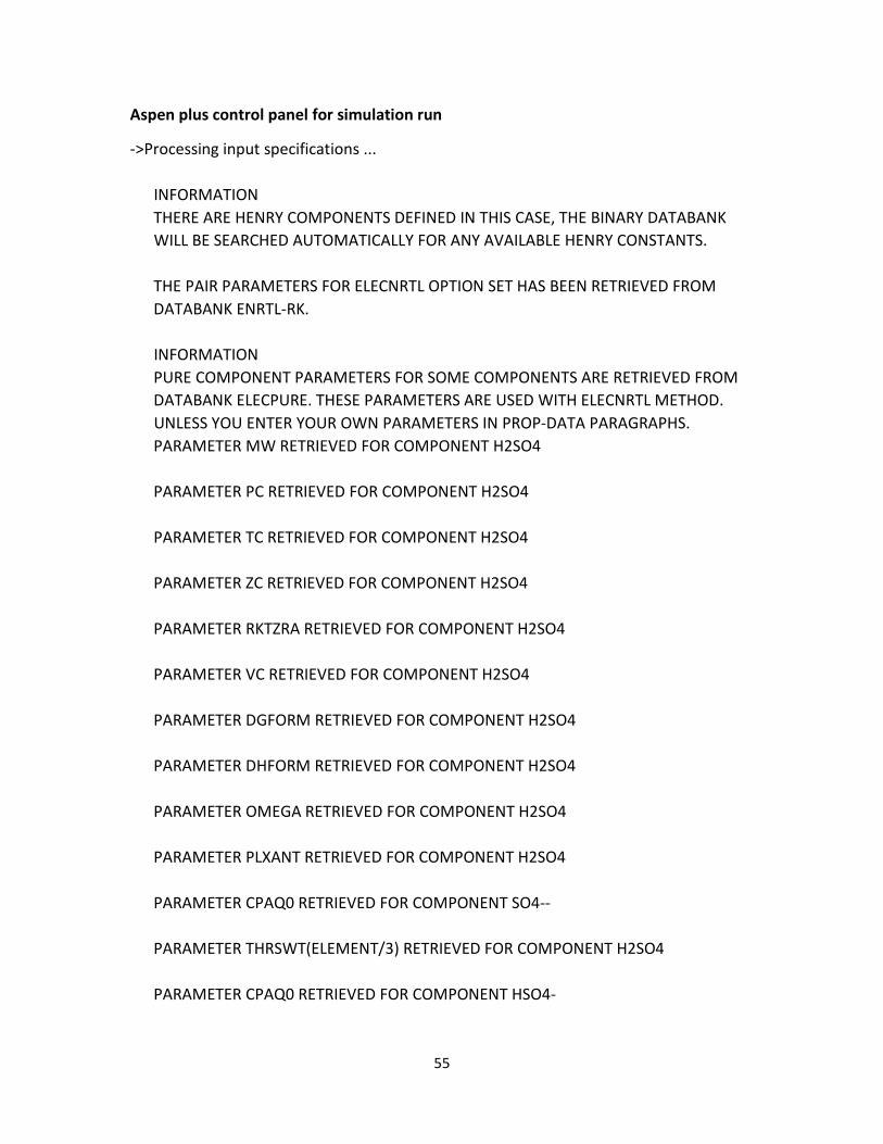
Aspen plus control panel for simulation run

->Processing input specifications ...

INFORMATION

THERE ARE HENRY COMPONENTS DEFINED IN THIS CASE, THE BINARY DATABANK

WILL BE SEARCHED AUTOMATICALLY FOR ANY AVAILABLE HENRY CONSTANTS.

THE PAIR PARAMETERS FOR ELECNRTL OPTION SET HAS BEEN RETRIEVED FROM

DATABANK ENRTL-RK.

INFORMATION

PURE COMPONENT PARAMETERS FOR SOME COMPONENTS ARE RETRIEVED FROM

DATABANK ELECPURE. THESE PARAMETERS ARE USED WITH ELECNRTL METHOD.

UNLESS YOU ENTER YOUR OWN PARAMETERS IN PROP-DATA PARAGRAPHS.

PARAMETER MW RETRIEVED FOR COMPONENT H2SO4

PARAMETER PC RETRIEVED FOR COMPONENT H2SO4

PARAMETER TC RETRIEVED FOR COMPONENT H2SO4

PARAMETER ZC RETRIEVED FOR COMPONENT H2SO4

PARAMETER RKTZRA RETRIEVED FOR COMPONENT H2SO4

PARAMETER VC RETRIEVED FOR COMPONENT H2SO4

PARAMETER DGFORM RETRIEVED FOR COMPONENT H2SO4

PARAMETER DHFORM RETRIEVED FOR COMPONENT H2SO4

PARAMETER OMEGA RETRIEVED FOR COMPONENT H2SO4

PARAMETER PLXANT RETRIEVED FOR COMPONENT H2SO4

PARAMETER CPAQ0 RETRIEVED FOR COMPONENT SO4--

PARAMETER THRSWT(ELEMENT/3) RETRIEVED FOR COMPONENT H2SO4

PARAMETER CPAQ0 RETRIEVED FOR COMPONENT HSO4-

56

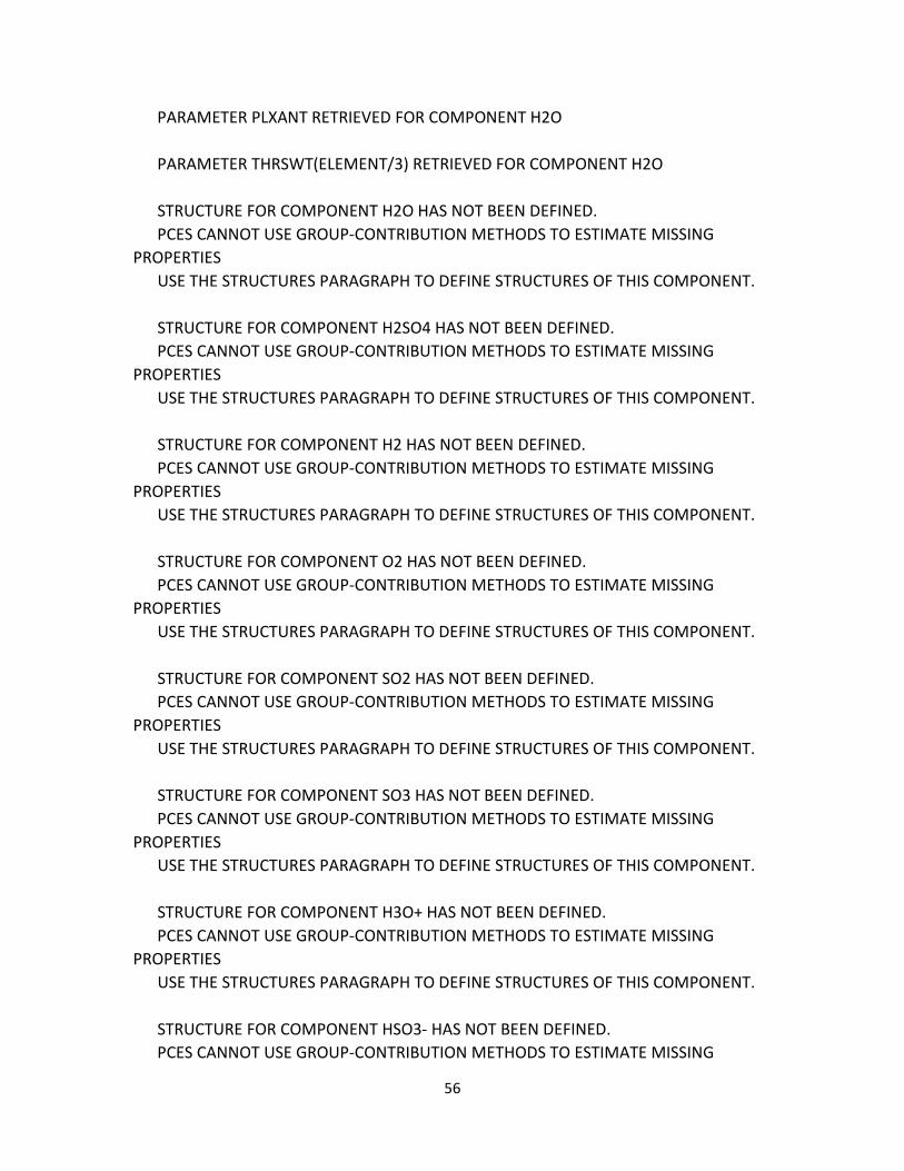
PARAMETER PLXANT RETRIEVED FOR COMPONENT H2O

PARAMETER THRSWT(ELEMENT/3) RETRIEVED FOR COMPONENT H2O

STRUCTURE FOR COMPONENT H2O HAS NOT BEEN DEFINED.

PCES CANNOT USE GROUP-CONTRIBUTION METHODS TO ESTIMATE MISSING

PROPERTIES

USE THE STRUCTURES PARAGRAPH TO DEFINE STRUCTURES OF THIS COMPONENT.

STRUCTURE FOR COMPONENT H2SO4 HAS NOT BEEN DEFINED.


PROPERTIES


STRUCTURE FOR COMPONENT H2 HAS NOT BEEN DEFINED.


PROPERTIES


STRUCTURE FOR COMPONENT O2 HAS NOT BEEN DEFINED.


PROPERTIES


STRUCTURE FOR COMPONENT SO2 HAS NOT BEEN DEFINED.


PROPERTIES


STRUCTURE FOR COMPONENT SO3 HAS NOT BEEN DEFINED.


PROPERTIES


STRUCTURE FOR COMPONENT H3O+ HAS NOT BEEN DEFINED.


PROPERTIES


STRUCTURE FOR COMPONENT HSO3- HAS NOT BEEN DEFINED.


57

PROPERTIES


STRUCTURE FOR COMPONENT HSO4- HAS NOT BEEN DEFINED.


PROPERTIES


STRUCTURE FOR COMPONENT SO3-- HAS NOT BEEN DEFINED.


PROPERTIES


STRUCTURE FOR COMPONENT SO4-- HAS NOT BEEN DEFINED.


PROPERTIES


* WARNING IN PHYSICAL PROPERTY SYSTEM

UNSYMMETRIC ELECTROLYTE NRTL MODEL GMENRTLQ HAS MISSING PARAMETERS:

Dielectric constant (CPDIEC) MISSING FOR SO3 . CPDIEC OF WATER

WILL BE ASSUMED.

* WARNING IN PHYSICAL PROPERTY SYSTEM

NRTL BINARY PARAMETERS FOR ALL COMPONENT PAIRS ARE ZERO,

YOUR RESULTS MAY NOT BE ACCURATE. PLEASE REVIEW AND PROVIDE BINARY

PARAMETERS AS APPROPRIATE.

Flowsheet Analysis :

COMPUTATION ORDER FOR THE FLOWSHEET:

T1 P1 SHXCONC VAL1 SFLCONC SHXD1 P2 BAYOH DECOMP BAYOC

SHXRCVRB SCONDENS SFLDECO SHXD2 FLSEP1 CMPRSEP1 SHXSEP1

CMPRSEP2 SHXSEP2 FLSEP2 PSEP1 SHXSEP3 TSEP2 VAL3 KSEP

SPSEP1 HXSEP5 VSEP1 FLSEP3 VAL4 KDESOR PSEP2 HXSEP4 MIXSEP1

HXPREP2 VAL2 HPBFW LPBFW MPBFW

->Calculations begin ...

Block: T1 Model: MIXER

58

Block: P1 Model: PUMP

Block: SHXCONC Model: HEATER

Block: VAL1 Model: VALVE

Block: SFLCONC Model: FLASH2

Block: SHXD1 Model: HEATER


Block: BAYOH Model: RSTOIC

Block: DECOMP Model: RSTOIC

Block: BAYOC Model: HEATER

Block: SHXRCVRB Model: HEATER

Block: SCONDENS Model: HEATER

Block: SFLDECO Model: FLASH2


Block: FLSEP1 Model: FLASH2

Block: CMPRSEP1 Model: COMPR

Block: SHXSEP1 Model: HEATER

Block: CMPRSEP2 Model: COMPR



Block: PSEP1 Model: PUMP

59


Block: TSEP2 Model: MIXER


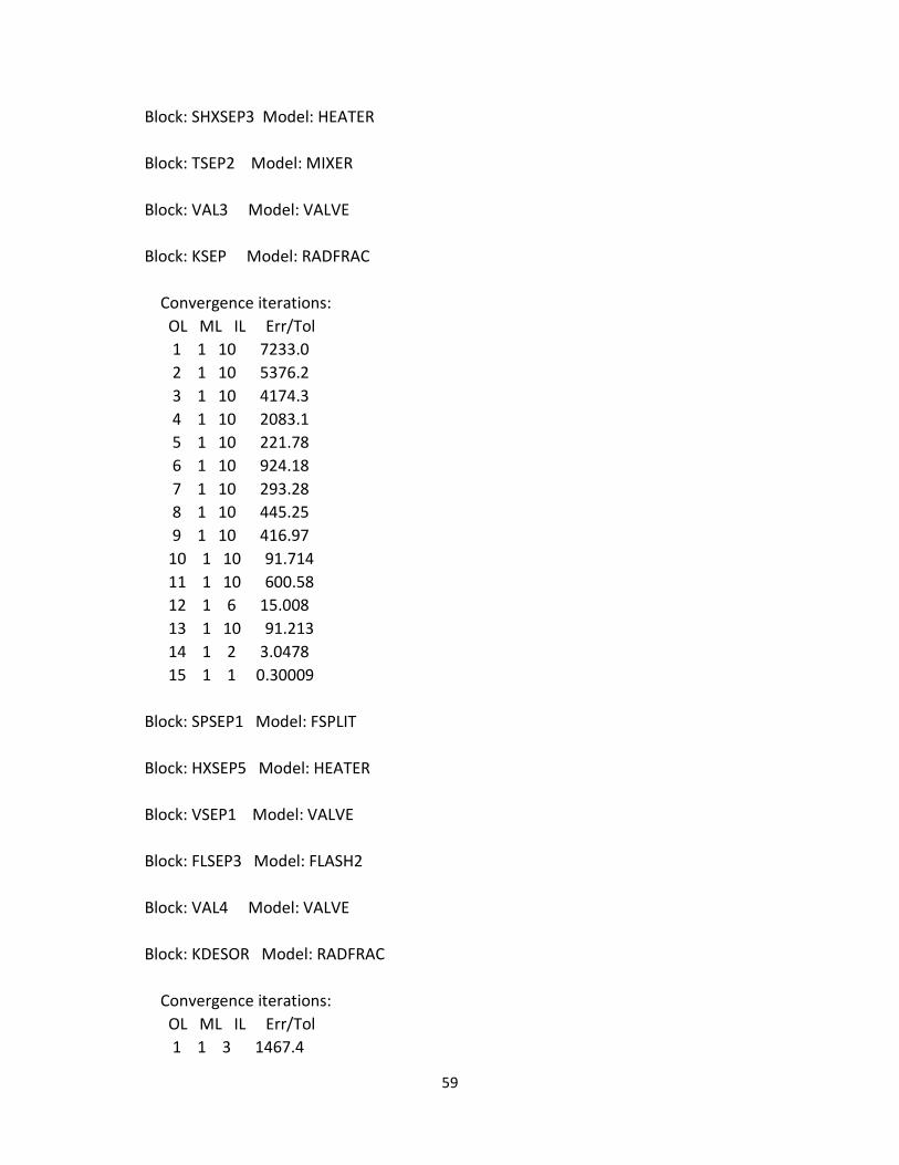
Block: KSEP Model: RADFRAC

Convergence iterations:

OL ML IL Err/Tol

1 1 10 7233.0

2 1 10 5376.2

3 1 10 4174.3

4 1 10 2083.1

5 1 10 221.78

6 1 10 924.18

7 1 10 293.28

8 1 10 445.25

9 1 10 416.97

10 1 10 91.714

11 1 10 600.58

12 1 6 15.008

13 1 10 91.213

14 1 2 3.0478

15 1 1 0.30009

Block: SPSEP1 Model: FSPLIT

Block: HXSEP5 Model: HEATER

Block: VSEP1 Model: VALVE



Block: KDESOR Model: RADFRAC

Convergence iterations:

OL ML IL Err/Tol

1 1 3 1467.4

60

2 1 2 209.92

3 1 1 42.254

4 1 1 5.5939

5 1 2 0.40024



Block: MIXSEP1 Model: MIXER

Block: HXPREP2 Model: HEATER


Utility HPBFW Model: GENERAL

Utility LPBFW Model: GENERAL

Utility MPBFW Model: GENERAL

->Generating block results ...

Block: BAYOC Model: HEATER

Block: SHXRCVRB Model: HEATER

Block: SCONDENS Model: HEATER

Block: SHXCONC Model: HEATER






61







Block: HXPREP2 Model: HEATER

->Simulation calculations completed ...

*** No Warnings were issued during Input Translation ***

*** Summary of Simulation Errors ***

Physical

Property System Simulation

Terminal Errors 0 0 0

Severe Errors 0 0 0

Errors 0 0 0

Warnings 2 0 0

** ERROR

CHEMISTRY (GLBAL) NOT CONVERGED; RMSERR= 0.2224 ; SUM OF DELX =

0.3945 .

dynamic simulation of a solar powered hybrid sulfur

Documents