dynamic stability enhancement of power system using fuzzy logic
TRANSCRIPT
Dynamic Stability Enhancement of
Power System Using Fuzzy Logic
Based Power System Stabilizer
Kamalesh Chandra Rout
Department of Electrical Engineering
National Institute of Technology,Rourkela
Rourkela-769008, Odisha, INDIA
May 2011

Dynamic Stability Enhancement of Power
System Using Fuzzy Logic Based Power
System Stabilizer
A thesis submitted in partial fulfillment of the
requirements for the degree of
Master of Technology by Researchin
Electrical Engineering
by
Kamalesh Chandra Rout(Roll-608EE309)
Under the Guidance of
Prof. P.C. PANDA
Department of Electrical Engineering
National Institute of Technology,Rourkela
Rourkela-769008, Odisha, INDIA
May 2011

Department of Electrical Engineering
National Institute of Technology, Rourkela
C E R T I F I C A T E
This is to certify that the thesis entitled ”Dynamic Stability Enhance-
ment of Power System Using Fuzzy Logic Based Power System
Stabilizer” by Mr. Kamalesh Chandra Rout, submitted to the Na-
tional Institute of Technology, Rourkela (Deemed University) for the award
of Master of Technology by Research in Electrical Engineering, is a record of
bonafide research work carried out by him in the Department of Electrical En-
gineering , under my supervision. I believe that this thesis fulfills part of the
requirements for the award of degree of Master of Technology by Research.The
results embodied in the thesis have not been submitted for the award of any
other degree elsewhere.
Place:Rourkela Prof. P.C. PANDA
Date:

DEDICATED TO MY BELOVED PARENTS WHO LED ME TO THIS
ACCOMPLISHMENT
Acknowledgements
Words are inadequate to express the overwhelming sense of gratitude and
humble regards to my supervisor Prof. P.C. Panda, Professor, Department of
Electrical Engineering for his constant motivation, support, expert guidance,
constant supervision and constructive suggestion for the submission of my
progress report of thesis work ”Dynamic Stability Enhancement of Power
System Using Fuzzy Logic Based Power System Stabilizer”.
I express my gratitude to Prof. Bidyadhar Subudhi, Head of the De-
partment, for his help and support during my study. I am thankful for the
opportunity to be a member of National institute of technology of Electrical
Engineering Department. I express my gratitude to the members of Masters
Scrutiny Committee, Professors K.B. Mohanty, K.K. Mohapatra and G.K.
Panda for their advice and care.
I also thank all the teaching and non-teaching staff for their nice cooper-
ation to the students.
I would like to thank all whose direct and indirect support helped me
completing my thesis in time.
This report would have been impossible if not for the perpetual moral
support from my family members, and my friends. I would like to thank
them all.
Kamalesh Chandra Rout
Rourkela, May 2011
v


Abstract
Power systems are subjected to low frequency disturbances that might cause
loss of synchronism and an eventual breakdown of entire system. The oscil-
lations, which are typically in the frequency range of 0.2 to 3.0 Hz, might
be excited by the disturbances in the system or, in some cases, might even
build up spontaneously. These oscillations limit the power transmission ca-
pability of a network and, sometimes, even cause a loss of synchronism and
an eventual breakdown of the entire system. For this purpose, Power sys-
tem stabilizers (PSS) are used to generate supplementary control signals for
the excitation system in order to damp these low frequency power system
oscillations.
The use of power system stabilizers has become very common in operation
of large electric power systems. The conventional PSS which uses lead-lag
compensation, where gain settings designed for specific operating conditions,
is giving poor performance under different loading conditions. The constantly
changing nature of power system makes the design of CPSS a difficult task.
Therefore, it is very difficult to design a stabilizer that could present good
performance in all operating points of electric power systems. To overcome
the drawback of conventional power system stabilizer (CPSS), many tech-
niques such as fuzzy logic, genetic algorithm, neural network etc. have been
proposed in the literature.
In an attempt to cover a wide range of operating conditions, Fuzzy logic
based technique has been suggested as a possible solution to overcome the
vii

above problem, thereby using this technique complex system mathematical
model can be avoided, while giving good performance under different op-
erating conditions. Fuzzy Logic has the features of simple concept, easy
implementation, and computationally efficient. The fuzzy logic based power
system stabilizer model is evaluated on a single machine infinite bus power
system, and then the performance of Conventional power system stabilizer
(CPSS) and Fuzzy logic based Power system stabilizer (FLPSS) are com-
pared. Results presented in the thesis demonstrate that the fuzzy logic based
power system stabilizer design gives better performance than the Conven-
tional Power system stabilizer.

Contents
Contents i
List of Figures v
List of Tables viii
1 INTRODUCTION 1
1.1 Power System Stability . . . . . . . . . . . . . . . . . . . . . . . 1
1.1.1 Types of Oscillations . . . . . . . . . . . . . . . . . . . . . 4
1.1.2 Low Frequency Oscillations . . . . . . . . . . . . . . . . . 5
1.2 Literature Survey . . . . . . . . . . . . . . . . . . . . . . . . . . 5
1.2.1 Power System Stabilizer (PSS) . . . . . . . . . . . . . . . . 5
1.2.2 PID (Proportional-Integral-Derivative) Controller . . . . . 7
1.2.3 Genetic Algorithm . . . . . . . . . . . . . . . . . . . . . . 7
1.2.4 Fuzzy Logic Controller . . . . . . . . . . . . . . . . . . . . 8
1.2.5 Neuro-Fuzzy Inference System . . . . . . . . . . . . . . . . 10
1.3 Problem Statement . . . . . . . . . . . . . . . . . . . . . . . . . 10
1.4 Solution Methodology . . . . . . . . . . . . . . . . . . . . . . . . 11
1.5 Objectives of the Work . . . . . . . . . . . . . . . . . . . . . . . 11
1.6 Contributions of the Thesis . . . . . . . . . . . . . . . . . . . . . 12
2 MODELLING OF POWER SYSTEM 13
2.1 Introduction . . . . . . . . . . . . . . . . . . . . . . . . . . . . . 13
2.2 Single Machine Infinite Bus (SMIB) Model . . . . . . . . . . . . 13
i

CONTENTS ii
2.2.1 Classical Model Representation of the Generator . . . . . . 14
2.3 Effects of Synchronous Machine Field Circuit Dynamics . . . . . 17
2.4 Representation of Saturation in Stability Studies . . . . . . . . . 21
2.5 Effects of Excitation system . . . . . . . . . . . . . . . . . . . . 22
2.6 Prime Mover and Governing System Models . . . . . . . . . . . 30
2.7 Power System Stabilizer (PSS) Model . . . . . . . . . . . . . . . 33
3 CONVENTIONAL POWER SYSTEM STABILIZERS 40
3.1 Introduction . . . . . . . . . . . . . . . . . . . . . . . . . . . . . 40
3.2 Conventional Power System Stabilizer Design . . . . . . . . . . . 40
3.3 Conclusion . . . . . . . . . . . . . . . . . . . . . . . . . . . . . . 48
4 DESIGN OF FUZZY LOGIC BASED PSS 50
4.1 Introduction . . . . . . . . . . . . . . . . . . . . . . . . . . . . . 50
4.2 Fuzzy sets . . . . . . . . . . . . . . . . . . . . . . . . . . . . . . 52
4.3 Membership functions . . . . . . . . . . . . . . . . . . . . . . . 52
4.3.1 Triangular Membership Function . . . . . . . . . . . . . . 53
4.3.2 Gaussian Membership Function . . . . . . . . . . . . . . . 54
4.3.3 Trapezoidal Membership Function . . . . . . . . . . . . . . 54
4.3.4 Sigmoidal Membership Function . . . . . . . . . . . . . . . 55
4.3.5 Generalized bell Membership Function . . . . . . . . . . . 56
4.4 Fuzzy Systems . . . . . . . . . . . . . . . . . . . . . . . . . . . . 57
4.5 Implication Methods . . . . . . . . . . . . . . . . . . . . . . . . 58
4.5.1 Mamdani Fuzzy Model . . . . . . . . . . . . . . . . . . . 59
4.5.2 Sugeno fuzzy model . . . . . . . . . . . . . . . . . . . . . . 59
4.6 Defuzzification Methods . . . . . . . . . . . . . . . . . . . . . . 60
4.6.1 Centroid Method . . . . . . . . . . . . . . . . . . . . . . . 60
4.6.2 Centre of Sums (COS) Method . . . . . . . . . . . . . . . 61
4.6.3 Mean of Maxima (MOM) Method . . . . . . . . . . . . . . 61
4.7 Design of Fuzzy Logic Based PSS . . . . . . . . . . . . . . . . . 61
4.7.1 Input/output Variables . . . . . . . . . . . . . . . . . . . . 62

CONTENTS iii
5 RESULTS AND DISCUSSION 67
5.1 The Case Study . . . . . . . . . . . . . . . . . . . . . . . . . . . 67
5.2 Performance without Excitation System . . . . . . . . . . . . . . 68
5.3 Performance with Excitation System . . . . . . . . . . . . . . . 69
5.4 Performance with Conventional PSS . . . . . . . . . . . . . . . . 70
5.5 Performance with Fuzzy Logic Based PSS . . . . . . . . . . . . 71
5.6 Performance with different membership functions . . . . . . . . 72
5.7 Response for different operating conditions using Triangular MF 74
5.8 Comparison of Conventional PSS and Fuzzy Logic Based PSS . 75
6 CONCLUSION AND SUGGESTIONS FOR FUTURE WORK 79
6.1 Conclusion . . . . . . . . . . . . . . . . . . . . . . . . . . . . . . 79
6.2 Suggestions for future work . . . . . . . . . . . . . . . . . . . . . 80
Bibliography 81
A System Data 86

List of Abbreviations
Abbreviation Description
AVR Automatic Voltage RegulatorAEA Adaptive Evolutionary AlgorithmANFIS Adaptive Neuro-Fuzzy Inference SystemCPSS Conventional Power System StabilizerCOS Centre of SumFLPSS Fuzzy Logic Power System StabilizerFL Fuzzy LogicFRMG Fuzzy Reference Model GeneratorGN Generalized NeuronGA Genetic AlgorithmLFO Low Frequency OscillationMF Membership FunctionMOM Mean of MaximaMISO Multi Input Single OutputMRAC Model Reference Adaptive ControllerNN Neural NetworkPSS Power System StabilizerPI Proportional IntegralPID Proportional Integral DerivativeRFLPSS Robust Fuzzy Logic Power System StabilizerRNNC Recurrent Neural Network ControllerSMIB Single Machine Infinite BusSTR Self Tuning Regulator
iv
List of Figures
2.1 General Configuration of SMIB . . . . . . . . . . . . . . . . . . . . 13
2.2 Equivalent Circuit of SMIB . . . . . . . . . . . . . . . . . . . . . . 14
2.3 Classical model of the synchronous generator . . . . . . . . . . . . 14
2.4 Phasor diagram of machine quantities . . . . . . . . . . . . . . . . 16
2.5 Phasor diagram of relative position of synchronous machine variables 18
2.6 Block diagram of a synchronous generator excitation system . . . . 23
2.7 Block diagram of thyristor excitation system with AVR . . . . . . 24
2.8 Block diagram representation with excitation and AVR . . . . . . . 27
2.9 Governor Characteristic . . . . . . . . . . . . . . . . . . . . . . . . 31
2.10Speed governing system . . . . . . . . . . . . . . . . . . . . . . . . 32
2.11Block diagram of a governing system for a hydraulic turbine . . . . 33
2.12Block diagram of thyristor excitation system with AVR and PSS . 35
2.13Block diagram of thyristor excitation system with AVR and PSS . 36
3.1 Block diagram of PSS . . . . . . . . . . . . . . . . . . . . . . . . . 41
3.2 Power System Configuration . . . . . . . . . . . . . . . . . . . . . 41
3.3 Block diagram of a linear model of a synchronous machine with a PSS 42
3.4 Simplified block diagram to design a CPSS . . . . . . . . . . . . . 43
3.5 Compact block diagram to design a CPSS . . . . . . . . . . . . . . 44
3.6 Frequency response of the plant without PSS . . . . . . . . . . . . 46
3.7 Frequency response of the CPSS (Gp(jω)) . . . . . . . . . . . . . 48
3.8 Frequency response of log magnitude of G(jω) and 1�Gp(jω) . . . . 48
v

LIST OF FIGURES vi
3.9 Closed loop frequency response of the system with CPSS . . . . . . 49
4.1 Triangular Membership Function . . . . . . . . . . . . . . . . . . . 53
4.2 Gaussian Membership Function . . . . . . . . . . . . . . . . . . . . 54
4.3 Trapezoidal Membership Function . . . . . . . . . . . . . . . . . . 55
4.4 Sigmoidal Membership Function . . . . . . . . . . . . . . . . . . . 56
4.5 Generalized bell Membership Function . . . . . . . . . . . . . . . . 56
4.6 Block diagram of Fuzzy logic controller . . . . . . . . . . . . . . . 57
4.7 Basic Structure of Fuzzy Logic Controller . . . . . . . . . . . . . . 62
4.8 Membership function for speed deviation . . . . . . . . . . . . . . 63
4.9 Membership function for acceleration . . . . . . . . . . . . . . . . . 63
4.10Membership function for voltage . . . . . . . . . . . . . . . . . . . 64
5.1 Test System for Proposed Fuzzy Logic Based PSS . . . . . . . . . 67
5.2 response without excitation system . . . . . . . . . . . . . . . . . . 68
5.3 Response with excitation system for -ve K5 . . . . . . . . . . . . . 69
5.4 Response with excitation system for +ve K5 . . . . . . . . . . . . 69
5.5 Response with CPSS for -ve K5 . . . . . . . . . . . . . . . . . . . . 70
5.6 Response with CPSS for +ve K5 . . . . . . . . . . . . . . . . . . . 70
5.7 Variation of angular position with FLPSS for -ve K5 . . . . . . . . 71
5.8 Variation of angular position with FLPSS for +ve K5 . . . . . . . 71
5.9 Variation of angular speed with FLPSS for -ve K5 . . . . . . . . . 72
5.10Variation of angular speed with FLPSS for +ve K5 . . . . . . . . . 72
5.11Angular position of different membership function for +ve K5 . . . 73
5.12Angular speed of different membership function for +ve K5 . . . . 73
5.13Angular position of different membership function for -ve K5 . . . 74
5.14Angular speed of different membership function for -ve K5 . . . . . 74
5.15Angular position for different operating conditions for -ve K5 . . . 75
5.16Angular position for different operating conditions for +ve K5 . . . 75
5.17Angular speed for different operating conditions for -ve K5 . . . . . 76
5.18Angular speed for different operating conditions for +ve K5 . . . . 76

LIST OF FIGURES vii
5.19Comparison of angular position between CPSS and FLPSS for -ve K5 77
5.20Comparison of angular position between CPSS and FLPSS for +ve K5 77
5.21Comparison of angular speed between CPSS and FLPSS for -ve K5 78
5.22Comparison of angular speed between CPSS and FLPSS for +ve K5 78

List of Tables
4.1 Membership functions for fuzzy variables . . . . . . . . . . . . . . 63
viii
Chapter 1
INTRODUCTION
1.1 Power System Stability
Power system stability is the tendency of a power system to develop restor-
ing forces equal to or greater than the disturbing forces to maintain the
state of equilibrium. Since power systems rely on synchronous machines for
generation of electrical power, a necessary condition for satisfactory system
operation is that all synchronous machines remain in synchronism. This as-
pect of stability is influenced by the dynamics of generator rotor angles and
power-angle relationships.
The power system is a dynamic system. The electrical power systems
today are no longer operated as isolated systems, but as interconnected sys-
tems which may include thousands of electric elements and be spread over
vast geographical areas. There are many advantages of interconnected power
systems
• Provide large blocks of power and increase reliability of the system.
• Reduce the number of machines which are required both for operation
at peak load and required as spinning reserve to take care of a sudden
change of load.
• Provide economical source of power to consumers.
1
CHAPTER 1. INTRODUCTION 2
On the other hand there are disadvantages of using interconnected power
systems. The interconnecting ties between neighboring power systems are
relatively weak when compared to the connections within the system. It
easily leads to low frequency inter oscillation. Many of the early instances
of oscillation instability occur at low frequencies when interconnections are
made. Power system stability can be classified into three categories.
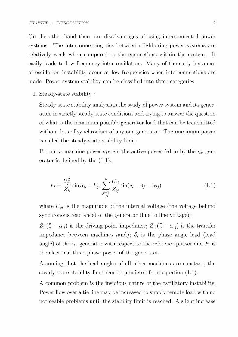
1. Steady-state stability :
Steady-state stability analysis is the study of power system and its gener-
ators in strictly steady state conditions and trying to answer the question
of what is the maximum possible generator load that can be transmitted
without loss of synchronism of any one generator. The maximum power
is called the steady-state stability limit.
For an n- machine power system the active power fed in by the ith gen-
erator is defined by the (1.1).
Pi =U 2
pi
Ziisin αii + Upi
n∑
j=1i 6=i
Upi
Zijsin(δi − δj − αij) (1.1)
where Upi is the magnitude of the internal voltage (the voltage behind
synchronous reactance) of the generator (line to line voltage);
Zii(π2 − αii) is the driving point impedance; Zij(
π2 − αij) is the transfer
impedance between machines iandj; δi is the phase angle lead (load
angle) of the ith generator with respect to the reference phasor and Pi is
the electrical three phase power of the generator.
Assuming that the load angles of all other machines are constant, the
steady-state stability limit can be predicted from equation (1.1).
A common problem is the insidious nature of the oscillatory instability.
Power flow over a tie line may be increased to supply remote load with no
noticeable problems until the stability limit is reached. A slight increase
CHAPTER 1. INTRODUCTION 3
in power flow beyond this limit results in oscillations in which amplitude
increases quickly with no need for any system fault. At best system non-
linearity limit oscillation amplitude. At worst, the oscillation amplitudes
reach levels at which protective relays trip lines and generation, and this
in turn causes partial or total system collapse [43].
2. Transient stability :
Transient stability is the ability of the power system to maintain syn-
chronism when subjected to a sudden and large disturbance within a
small time such as a fault on transmission facilities, loss of generation or
loss of a large load [4].
The system response to such disturbances involves large excursions of
generator rotor angles, power flows, bus voltages etc.
It is a fast phenomenon usually occurring within 1 second for a generator
close to the cause of disturbance such as 3-phase to ground fault, line to
ground fault etc.
3. Dynamic Stability :
A system is said to be dynamically stable if the oscillations do not acquire
more than certain amplitude and die out quickly. Dynamic stability is
a concept used in the study of transient conditions in power systems.
Any electrical disturbances in a power system will cause electromechan-
ical transient processes. Besides the electrical transient phenomena pro-
duced, the power balance of the generating units is always disturbed, and
thereby mechanical oscillations of machine rotors follow the disturbance
[38].
To describe the transient phenomena, the well-known swing equation of
the synchronous generators, derived from the torque equation for syn-
CHAPTER 1. INTRODUCTION 4
chronous machine, can be used:
Twid2δi
dt2= PMi −Di
d
dtδi − PEi (1.2)
where Twi is the impulse moment of the rotor of the generating unit,Di
is the damping coefficient (representing the mechanical as well as the
electrical damping effect), δi is the phase angle (load angle), PMi is the
turbine power applied to rotor and PEi is the electrical power output
from the stator.
1.1.1 Types of Oscillations
The disturbances occurring in power system include electromechanical oscil-
lations of electrical generators. These oscillations are also called power swings
and these must be effectively damped to maintain the system stability. Elec-
tromechanical oscillations can be classified in four main categories.
1. Local oscillations: - Between a unit and rest of generating station and
between the later and rest of power system. Their frequency typically
ranges from 0.2 Hz to 2.5 Hz.
2. Interplant oscillations: - Between two electrically close generating plants.
Frequency can vary from 1 Hz to 2 Hz.
3. Interarea oscillations: - Between two major groups of generating plants.
Frequencies are typically in the range of 0.2 Hz to 0.8 Hz, generally called
low frequency oscillations.
4. Global oscillations: - Characterized by a common in phase oscillations
of all generators as found on an isolated system. The frequency of such
global mode is typically under 0.2 Hz.
CHAPTER 1. INTRODUCTION 5
1.1.2 Low Frequency Oscillations
Low frequency oscillations (LFOs) are generator rotor angle oscillations hav-
ing a frequency between 0.1 Hz to 3.0 Hz and are defined by how they are
created or where they are located in the power system. The use of high gain
exciters, poorly turned generation excitation, HVDC converters may create
LFOs with negative damping; this is a small-signal stability problem. The
mitigation of these oscillations is commonly performed with ”supplementary
stabilizing signals” and the networks used to generate these signals have come
to be known as ”power system stabilizer” networks. LFOs include local plant
modes, control modes, torsional modes induced by the interaction between
the mechanical and electrical modes of a turbine-generator system, and inter-
area modes, which may be caused by either high gain exciters or heavy power
transfers across weak tie lines.
Low frequency oscillations can be created by small disturbances in the
system, such as changes in the load, and are normally analyzed through the
small-signal stability (linear response) of the power system. These small
disturbances lead to a steady increase or decrease in generator rotor angle
caused by the lack of synchronizing torque, or to rotor oscillations of in-
creasing amplitude due to a lack of sufficient damping torque. The most
typical instability is the lack of a sufficient damping torque on the rotor’s low
frequency oscillations.
1.2 Literature Survey
1.2.1 Power System Stabilizer (PSS)
A. Dysko, W.E. Leithead and J. O’Reilly [18] have described a step-by-step
coordinated design procedure for power system stabilizers (PSSs) and auto-
matic voltage regulators (AVRs) in a strongly coupled system. The proposed
coordinated PSS/AVR design procedure is established within a frequency-
domain framework. Chow and Sanchez-Gasca [13] proposes a power system

CHAPTER 1. INTRODUCTION 6
stabilizer using pole placement technique and this work is carried by Yu and
Li [55] for a nine bus system. G Guralla, R Padhi and I Sen [23] have proposed
a method of designing fixed parameter decentralized power system stabilizers
(PSS) for interconnected multi machine power systems. Here Heffron - Philips
model is used to decide the structure of the PSS compensator and tune its
parameters at each machine in the multi machine environment. A. Chatter-
jee, S.P. Ghosal, and V. Mukherjee [9] have described a comparative transient
performance of single-input conventional power system stabilizer (CPSS) and
dual-input power system stabilizer (PSS), namely PSS4B. An experience of
dynamic instability [50] has analyzed in this paper. The method of analysis
was to determine stability by the calculation of the Eigen values of the system.
Explanation is provided [6] regarding small signal stability, high impedance
transmission lines, line loading, and high gain, fast acting excitation sys-
tems. An experience in assigning PSS projects [14] has discussed in an under
graduate control design course to provide students with a challenging de-
sign problem using three different techniques (root-locus, frequency-domain,
state-space) and to expose them to power system engineering. A generalized
neuron (GN) that requires much smaller training data and shorter training
time has developed and by taking benefit of these characteristics of the GN,
a new power system stabilizer is proposed [10]. Wah-Chun Chan, Yuan-Yih
Hsu [8] presents a technique for designing an optimal variable structure sta-
bilizer for improving the dynamic stability of power systems by increasing
the damping torque of the synchronous machine in the system. De Mello
[15] has explored the phenomenon of stability of synchronous machines un-
der small perturbations by examining the case of single machine connected
to an infinite bus through external reactance. The design of PSS for single
machine connected to an infinite bus has been described [19] using fast out-
put sampling feedback. A step-up transformer is used to set up a modified
Heffron-Philips (ModHP) model. The PSS design based on this model uti-
lizes signals available within the generating station [22]. An augmented PSS

CHAPTER 1. INTRODUCTION 7
[35] is described which extends the performance capabilities into the weak
tie-line case. E.V Larsen and D.A Swann [31] have presented in their 3 pa-
per titled ’Applying power system stabilizer - I, II, III’ the history of power
system stabilizer and its role in a power system. Practical means have been
developed using Eigen value [16] analysis techniques to guide the selection
process. An extended quasi-steady-state model [52] has presented that in-
cludes low-frequency interarea oscillations which can be used effectively for
the design of power system stabilizers. Wlfred Watson and Gerald Manchur
[53] has suggested that the use of high speed excitation for generator static
excitation systems results in decreased damping, which has detrimental im-
pact on steady state stability, i.e. it may be lost even at normal full load
operation.
1.2.2 PID (Proportional-Integral-Derivative) Controller
Radman and Smaili [40] have proposed the PID based power system stabi-
lizer and Wu and Hsu [12] have proposed the self tuning PID power system
stabilizer for a multi machine power system. M. Dobrescu, I. Kamwa [17]
in their paper has described a PID (proportional-integral-derivative) type
FLPSS with adjustable gains added outside in order to keep a simple struc-
ture. In order to validate the FLPSS, it has been compared with two reference
stabilizers; the IEEE PSS4B and IEEE PSS2B form the IEEE STD 421.5. A.
Jalilvand, R. Aghmasheh and E. Khalkhali in their paper [27] have described
the tuning of Proportional Integral Derivative power system stabilizers (PID-
PSS) using Artificial intelligence (AI) technique.
1.2.3 Genetic Algorithm
G.H. Hwang [26] have described a design of fuzzy power system stabilizer
(FPSS) using an adaptive evolutionary algorithm (AEA). AEA consists of
Genetic Algorithm (GA) for a global search capability and evolution strategy
(ES) for a local search in an adaptive manner. AEA is used to optimize the

CHAPTER 1. INTRODUCTION 8
membership functions and scaling factors of FPSS. A.S. Al-Hinai and S.M.
Al-Hinai [2] have used Genetic Algorithm for a proper design of a power
system stabilizer. A Babaei, S.E. Razavi, S.A. Kamali, A. Gholami [5] have
used a modified Genetic Algorithm for suitable design of stabilizer.
1.2.4 Fuzzy Logic Controller
Lin [32] proposed a fuzzy logic power system stabilizer which could shorten
the tuning process of fuzzy rules and membership functions. The proposed
PSS has two stages, first stage develops a proportional derivative type PSS,
in the second stage it is transformed into FLPSS. Roosta, A.R, [44] have
described three proposed types of fuzzy control algorithms and tested in the
case of single machine connected to the network for various types of distur-
bance. S.A. Taher has proposed a novel robust fuzzy logic power system
stabilizer (RFLPSS). Here to provide robustness, additional signal namely
speed is used as inputs to RFLPSS enabling appropriate gain adjustments
[48]. M.L. Kothari, T. Kumar [29] have presented a new approach for design-
ing a fuzzy logic power system stabilizer such that it improves both transient
and dynamic stabilities. Here they have considered FLPSS based on 3, 5 and
7 MFs of Gaussian shape. T. Hussein [25] has described an indirect variable-
structure adaptive fuzzy controller as a power system stabilizer (IDVSFPSS)
to damp inter-area modes of oscillation following disturbances in power sys-
tems. S.K. Yee and J.V. Milanovic [54] have proposed a decentralized fuzzy
logic controller using a systematic analytical method based on a performance
index. F. Rashidi [42] has described a fuzzy sliding mode controller in which
a simple fuzzy inference mechanism is used to estimate the upper bound of
uncertainties. Kamalasadan, S and Swann, G [28] have proposed a fuzzy
model reference adaptive controller uses a fuzzy reference model generator
(FRMG) in parallel with the model reference adaptive controller (MRAC).
N. Gupta and S.K. Jain [21] have described the performance of single machine
infinite bus system with fuzzy power system stabilizer. Here the generator is

CHAPTER 1. INTRODUCTION 9
represented by the standard K-coefficients as second order systems and the
performance is investigated for Trapezoidal, Triangular Gaussian membership
functions of input and output variables. M. Ramirez, O.P. Malik [41] have de-
scribed a simplified fuzzy logic controller (SFLC) with a significantly reduced
set of fuzzy rules, small number of tuning parameters and simple control al-
gorithm and structure. T. Hussein [47] has presented a robust adaptive fuzzy
controller as a power system stabilizer (RFPSS) to damp inter-area modes of
oscillation following disturbances in power systems. Matsuki et al. [36] de-
scribed the process of determination of optimal fuzzy control parameters by
trial and error. R. Gupya, D.K. Sambariya, R. Gunjan [20] have discussed a
study of fuzzy logic power system stabilizer (PSS) for stability enhancement
of a multi machine power system. H.M. Behbehani [7] have used fuzzy logic
principles to develop supervisory power system stabilizers (SPSS) to enhance
damping of inter-area oscillations to improve stability and reliability of power
system subjected to disturbances. N.Nallathambi presents a study of fuzzy
logic power system stabilizer for stability enhancement of a two-area four
machine system [37]. Park and Lee [39] proposed a self organizing power
system stabilizer where the rules are generated automatically and rule base
updated online by self organizing procedure. Lu J. [33] proposed a fuzzy logic
based adaptive power system stabilizer. A. Singh has described the design
of a fuzzy logic based controller to counter the small-signal oscillatory insta-
bility in power systems [45]. K.L. Al-Olimat [3] has presented a self tuning
regulator (STR) with multi identification models and a minimum variance
controller that utilizes fuzzy logic switching. Taliyat et al. [49] proposed an
augmented fuzzy PSS. Hussein et al. [24] proposed self tuning power sys-
tem stabilizer in which two tuning parameters are introduced to tune fuzzy
logic PSS. Abdelazim and Malik [1] proposed a self learning fuzzy logic power
system stabilizer.

CHAPTER 1. INTRODUCTION 10
1.2.5 Neuro-Fuzzy Inference System
M. F. Othman, M. Mahfouf and D.A. Linkens, have described the design
procedure for a fuzzy logic based power system stabilizer (FLPSS) and adap-
tive neuro-fuzzy inference system (ANFIS) and investigates their robustness
for a multi-machine power system. Speed deviation of a machine and its
derivative are chosen as the input signals to the FLPSS [34]. Vani, M.U,
Raju, G.S and Prasad, K.R.L [51] in their paper have presented a step-by-
step design methodology of an adaptive Neuro-Fuzzy inference system and
optimization methods based automatic voltage regulator and power system
stabilizer. Chun-Jung Chen [11] has presented an adaptive power system sta-
bilizer (PSS) which consists of a recurrent neural network controller (RNNC)
and a compensator to damp the oscillations of power system. The function
of RNNC is to supply an adaptive control signal to the exciter or governor,
which can damp most of the power system’s oscillations. Sumina D. [46] have
presented the usage of neural network (NN) based excitation control on single
machine infinite bus. The proposed feed forward neural network integrates a
voltage regulator and a power system stabilizer.
1.3 Problem Statement
Some of the earliest power system stability problems included spontaneous
power system oscillations at low frequencies. These low frequency oscilla-
tions (LFOs) are related to the small signal stability of a power system and
are detrimental to the goals of maximum power transfer and power system
security. Once the solution of using damper windings on the generator rotors
and turbines to control these oscillations was found to be satisfactory, the
stability problem was thereby disregarded for some time. However, as power
systems began to be operated closer to their stability limits, the weakness
of a synchronizing torque among the generators was recognized as a ma-
jor cause of system instability. Automatic voltage regulators (AVRs) helped

CHAPTER 1. INTRODUCTION 11
to improve the steady-state stability of the power systems. But with the
creation of large, interconnected power systems, another concern was the
transfer of large amounts of power across extremely long transmission lines.
The addition of a supplementary controller into the control loop, such as the
introduction of conventional power system stabilizers (CPSSs) to the AVRs
on the generators, provides the means to reduce the inhibiting effects of low
frequency oscillations. The conventional power system stabilizers work well
at the particular network configuration and steady state conditions for which
they were designed. Once conditions change the performance degrades.
The conventional power system stabilizer such as lead-lag, proportional
integral (PI) power system stabilizer, proportional integral derivative (PID)
power system stabilizer operates at a certain point. So the disadvantage of
this type of stabilizer is they cannot operate under different disturbances.
This can be overcome by a PSS design based on Fuzzy logic technique.
1.4 Solution Methodology
To overcome the drawbacks of conventional power system stabilizer (CPSS),
numerous techniques have been proposed in the literature. In this thesis
work, the conventional PSS’s effect on the system damping is then compared
with a fuzzy logic based PSS while applied to a single machine infinite bus
(SMIB) power system. For the conventional design state space representation
is used here.
1.5 Objectives of the Work
The objectives of the project are
• To study the nature of power system stability, excitation system, au-
tomatic voltage regulator for synchronous generator and power system
stabilizer.

CHAPTER 1. INTRODUCTION 12
• To develop a fuzzy logic based power system stabilizer which will make
the system quickly stable when fault occurred in the transmission line.
• By using simulation to validate fuzzy logic based power system stabi-
lizer and its performance is compared with conventional power system
stabilizer and without power system stabilizer.
1.6 Contributions of the Thesis
Chapter 1 :
Presents the introduction to power system stability, low frequency oscilla-
tions, literature survey, and objective of the work and chapter wise contribu-
tion of the thesis.
Chapter 2 :
Presents the modelling of power system and formation of the state space
matrix of the single machine infinite bus (SMIB) system.
Chapter 3 :
Presents a frequency response method for the design of a conventional
power system stabilizer (CPSS) in the frequency domain.
Chapter 4 :
Presents briefly the fuzzy logic control theory, need for implementing fuzzy
controller. It also describes fuzzy logic based PSS.
Chapter 5 :
Presents results and discussions for without excitation system, with exci-
tation system only, with conventional PSS, with fuzzy logic based PSS and
a comparison between conventional PSS and fuzzy logic based PSS.
Chapter 6 :
Presents conclusion and suggestions for future work.

Chapter 2
MODELLING OF POWER SYSTEM
2.1 Introduction
For stability assessment of power system adequate mathematical models de-
scribing the system are needed. The models must be computationally efficient
and be able to represent the essential dynamics of the power system. The
mathematical model for small signal analysis of synchronous machine, exci-
tation system and the lead-lag power system stabilizer are briefly reviewed.
2.2 Single Machine Infinite Bus (SMIB) Model
The performance of a synchronous machine connected to a large system
through transmission lines has shown in Figure 2.1. The synchronous ma-
chine is vital for power system operation. The general system configuration of
synchronous machine connected to infinite bus through transmission network
can be represented as the Thevenin’s equivalent circuit.
tV
trX
BE
Figure 2.1: General Configuration of SMIB
13

CHAPTER 2. MODELLING OF POWER SYSTEM 14
At first the synchronous machine will be represented by the classical model.
Then, the model details will be increased to account for the effects of the dy-
namics of the field circuit and the excitation system. The block diagram rep-
resentation and torque-angle relationships will be used to analyze the system-
stability characteristics. The block diagram representation and torque-angle
relationships will be used to analyze the system-stability characteristics.
For the purpose of analysis, the system of Figure 2.1 may be reduced to
the form of Figure 2.2.
G Infinite bus
Figure 2.2: Equivalent Circuit of SMIB
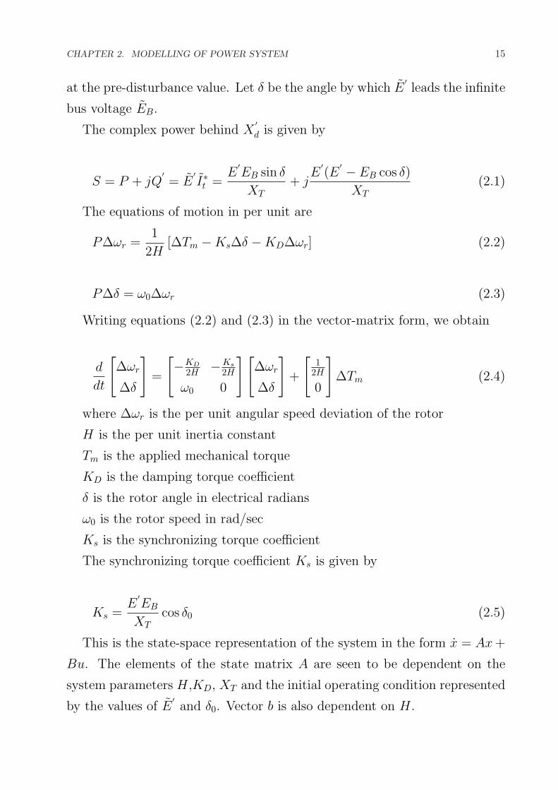
2.2.1 Classical Model Representation of the Generator
The classical model representation of the generator [30] and with all the
resistances neglected, the system representation is shown in Figure 2.3.
Figure 2.3: Classical model of the synchronous generator
In Figure 2.3, E′is the voltage behind X
′d, which is the direct axis transient
reactance of the generator. The magnitude of E′is assume to remain constant
CHAPTER 2. MODELLING OF POWER SYSTEM 15
at the pre-disturbance value. Let δ be the angle by which E′leads the infinite
bus voltage EB.
The complex power behind X′d is given by
S = P + jQ′= E
′I∗t =
E′EB sin δ
XT+ j
E′(E
′ − EB cos δ)
XT(2.1)
The equations of motion in per unit are
P∆ωr =1
2H[∆Tm −Ks∆δ −KD∆ωr] (2.2)
P∆δ = ω0∆ωr (2.3)
Writing equations (2.2) and (2.3) in the vector-matrix form, we obtain
d
dt
[∆ωr
∆δ
]=
[−KD
2H −Ks
2H
ω0 0
][∆ωr
∆δ
]+
[1
2H
0
]∆Tm (2.4)
where ∆ωr is the per unit angular speed deviation of the rotor
H is the per unit inertia constant
Tm is the applied mechanical torque
KD is the damping torque coefficient
δ is the rotor angle in electrical radians
ω0 is the rotor speed in rad/sec
Ks is the synchronizing torque coefficient
The synchronizing torque coefficient Ks is given by
Ks =E′EB
XTcos δ0 (2.5)
This is the state-space representation of the system in the form x = Ax +
Bu. The elements of the state matrix A are seen to be dependent on the
system parameters H,KD, XT and the initial operating condition represented
by the values of E′and δ0. Vector b is also dependent on H.
CHAPTER 2. MODELLING OF POWER SYSTEM 16
Therefore, the undamped natural frequency is
ωn =
√Ks
ω0
2H(2.6)
ζ =1
2
KD
2Hωn=
1
2
KD√Ks2Hω0
(2.7)
As the synchronizing torque coefficient Ks increases, the natural frequency
increases and the damping ratio decreases. An increase in damping torque
coefficient KD increases the damping ratio, whereas an increase in inertia
constant decreases both ωn and ζ.
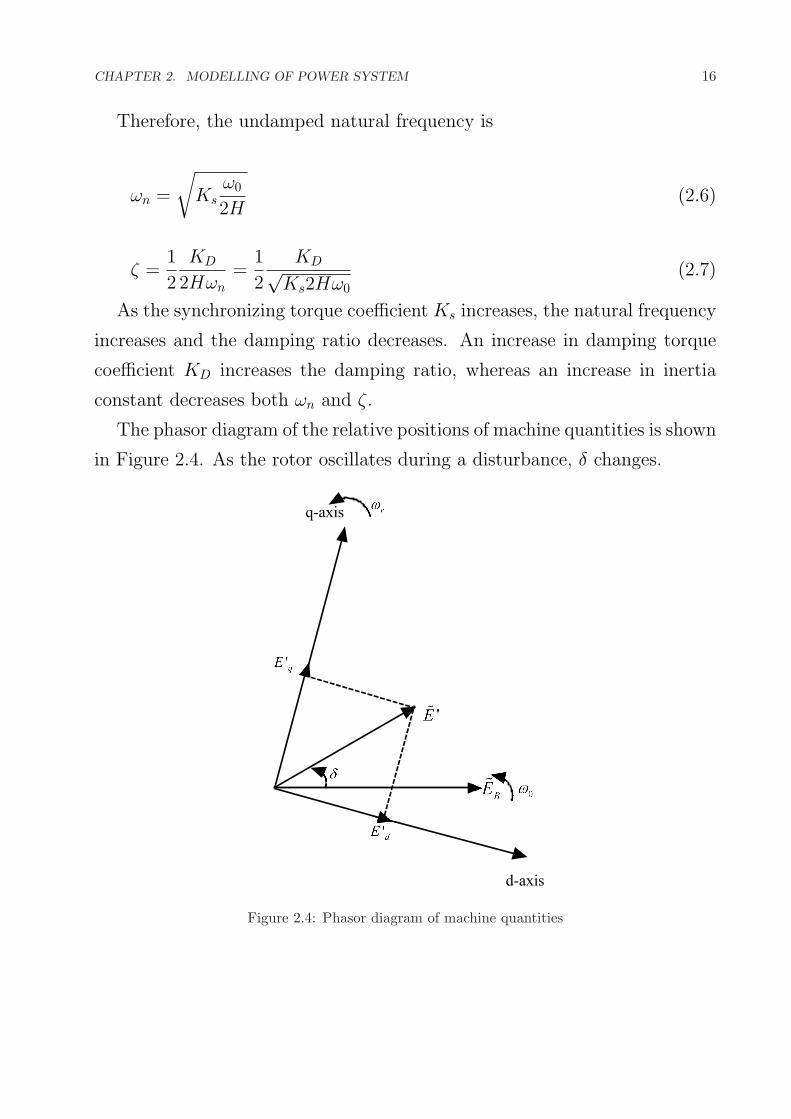
The phasor diagram of the relative positions of machine quantities is shown
in Figure 2.4. As the rotor oscillates during a disturbance, δ changes.
q-axis
d-axis
Figure 2.4: Phasor diagram of machine quantities
CHAPTER 2. MODELLING OF POWER SYSTEM 17
2.3 Effects of Synchronous Machine Field Circuit Dynamics
Now we consider the system performance including the effect of field flux
variations. Then we will develop the state-space model of the system by first
reducing the synchronous machine equations to an appropriate form and then
combining them with the network equations.
As in the case of the classical generator model, the linearised equations of
motion are
d
dt∆ωr =
1
2H(∆Tm −∆Te −KD∆ωr) (2.8)
d
dt∆δ = ω0∆ωr (2.9)
d
dt∆δ = ω0∆ωr (2.10)
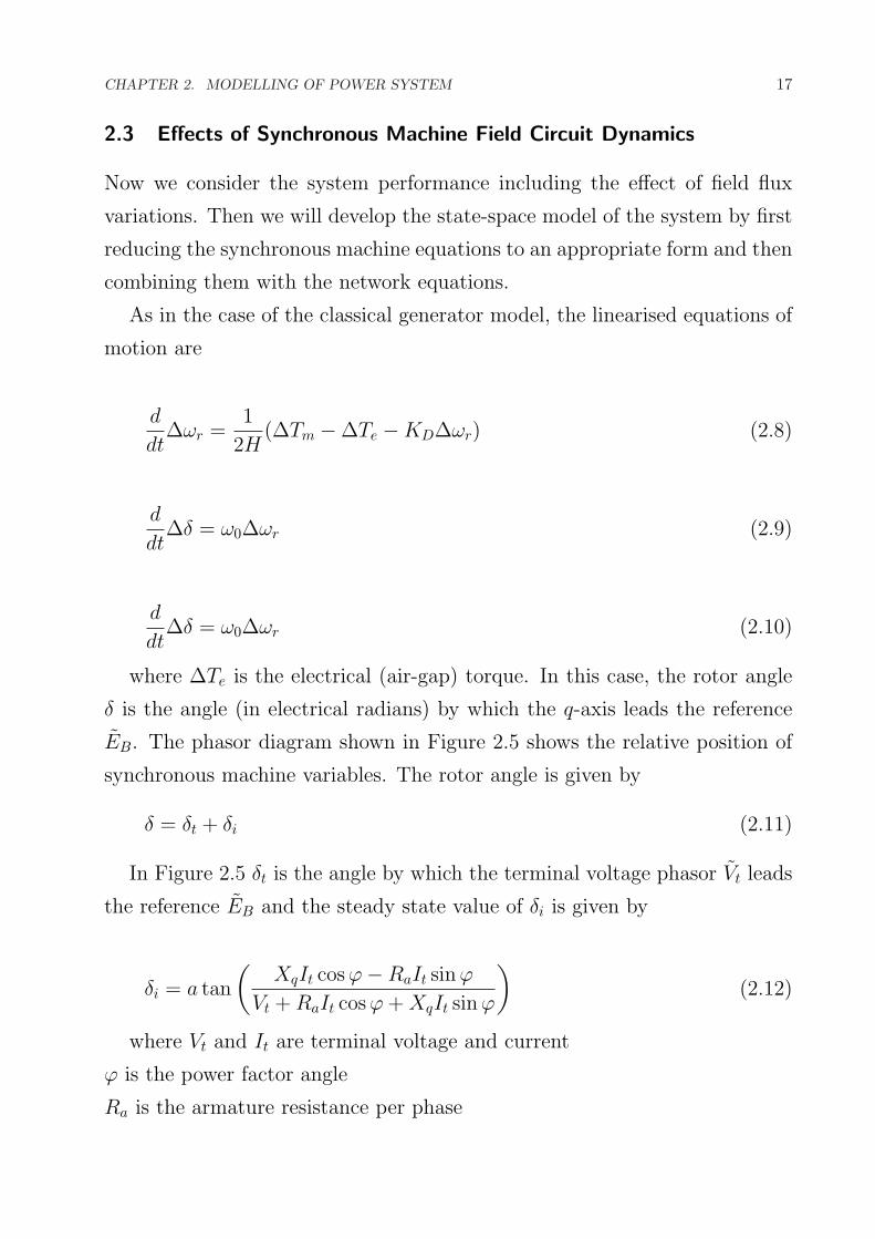
where ∆Te is the electrical (air-gap) torque. In this case, the rotor angle
δ is the angle (in electrical radians) by which the q-axis leads the reference
EB. The phasor diagram shown in Figure 2.5 shows the relative position of
synchronous machine variables. The rotor angle is given by
δ = δt + δi (2.11)
In Figure 2.5 δt is the angle by which the terminal voltage phasor Vt leads
the reference EB and the steady state value of δi is given by
δi = a tan
(XqIt cos ϕ−RaIt sin ϕ
Vt + RaIt cos ϕ + XqIt sin ϕ
)(2.12)
where Vt and It are terminal voltage and current
ϕ is the power factor angle
Ra is the armature resistance per phase

CHAPTER 2. MODELLING OF POWER SYSTEM 18
q-axis
d-axis
Figure 2.5: Phasor diagram of relative position of synchronous machine variables
Xq is the quadrature-axis synchronous reactance
The effect of field flux variations can be represented as
d
dt∆ψfd =
ω0Rfd
Ladu∆Efd − ω0Rfd∆ifd (2.13)
where ∆ψfd is the rotor circuit (field) flux linkage
Rfd is the rotor circuit resistance
Ladu is the unsaturated direct-axis manual inductance between stator and
rotor windings
Efd is the exciter output voltage
ifd is the field circuit current
In order to develop the complete system equations in the state-space form
∆Te and ∆ifd should be expressed in terms of the state variables as deter-
mined by the machine flux linkage equations and network equations. So we
CHAPTER 2. MODELLING OF POWER SYSTEM 19
can write that
∆ifd =1
Lfd
(1 + m2L
′ads − L
′ads
Lfd
)∆ψfd +
1
Lfdm1L
′ads∆δ (2.14)
where
L′ads =
LadsLfd
Lads + Lfd(2.15)
m1 =EB(XTq sin δ0 −RT cos δ0)
D(2.16)
m2 =XTq
D
(Lads
Lads + Lfd
)(2.17)
RT = Ra + RE (2.18)
XTq = Xtr + XE + (Laqs + Ll) (2.19)
XTd = Xtr + XE + (L′ads + Ll) (2.20)
D = R2T + XTqXTd (2.21)
where Xtr is the reactance of the transformer
RE is the Thevenin resistance of the network
XE is the Thevenin reactance of the network
Ra is the armature resistance
Ll is the leakage inductance of the stator
Lads is the saturated d-axis mutual inductance between stator and rotor wind-
ings
Laqs is the saturated q-axis mutual inductance between stator and rotor wind-
ings
Also we can derive that
∆Te = K1∆δ + K2∆ψfd (2.22)

CHAPTER 2. MODELLING OF POWER SYSTEM 20
K1 = n1(ψad0 + Laqsid0)−m1(ψaq0 + L′adsiq0) (2.23)
K2 = n2(ψad0 + Laqsid0)−m2(ψaq0 + L′aq0iq0) +
L′ads
Lfdiq0 (2.24)
Here
n1 =EB(RT sin δ0 −XTD cos δ0)
D(2.25)
n2 =RT
D
Lads
(Lads + Lfd)(2.26)
id0 =XTq
[ψfd0
(Lads
Lads+Lfd
)− EB cos δ0
]−RTEB sin δ0
D(2.27)
iq0 =RT
[ψfd0
(Lads
Lads+Lfd
)− EB cos δ0
]−XTdEB sin δ0
D(2.28)
ψad0 = L′ads
(ψfd0
Lfd− id0
)(2.29)
ψaq0 = −Laqsiq0 (2.30)
By substituting the expressions for ∆ifd and ∆Te given by equations (2.13)
and (2.21) into equations (2.8) and (2.12), the state-space representation of
the system is obtained as follows:
d
dt
∆ωr
∆δ
∆ψfd
=
a11 a12 a13
a21 0 0
0 a32 a33
∆ωr
∆δ
∆ψfd
+
b11
0
0
0
0
b32
[∆Tm
∆Efd
](2.31)
where
a11 = −KD
2H(2.32)
CHAPTER 2. MODELLING OF POWER SYSTEM 21
a12 = −K1
2H(2.33)
a13 = −K2
2H(2.34)
a21 = ω0 = 2Πf0 (2.35)
a32 = −ω0Rfd
Lfdm1L
′ads (2.36)
a33 = −ω0Rfd
Lfd
(m2L
′ads + 1− L
′ads
Lfd
)(2.37)
b11 =1
2H(2.38)
b32 =ω0Rfd
Ladu(2.39)
∆Tm and ∆Efd depend on prime mover and excitation controls. With
constant mechanical input torque ∆Tm= 0; with constant exciter output
voltage ∆Efd= 0.
2.4 Representation of Saturation in Stability Studies
For stability studies the following assumptions are made in the representation
of magnetic saturation.
• The leakage inductances are independent of saturation and only elements
that saturate are the mutual inductances and .
• The leakage fluxes do not contribute to the iron saturation and the sat-
uration is determined by the air-gap flux linkage.
• The saturation relationship between the resultant air-gap flux and the
mmf under loaded conditions is the same as under no-load conditions.

CHAPTER 2. MODELLING OF POWER SYSTEM 22
• There is no magnetic coupling between the d- and q-axes.
2.5 Effects of Excitation system
The main objective of the excitation system is to control the field current of
the synchronous machine. The field current is controlled so as to regulate the
terminal voltage of the machine. As the field circuit time constant is high
(of the order of a few seconds), fast control of the field current requires field
forcing. Thus exciter should have a high ceiling voltage which enables it to
operate transiently with voltage levels that are 3 to 4 times the normal. The
rate of change of voltage should also be fast. Because of the high reliability
required, unit exciter scheme is prevalent where each generating unit has its
individual exciter. From the power system view point, the excitation system
should contribute to effective control of voltage and enhancement of system
stability. It should be capable of responding rapidly to a disturbance so
as to enhance transient stability. In this dissertation, excitation control has
been assumed for the purpose of analysis. Fundamentally, simplest excitation
system consists of an exciter only. When the excitation system also performs
the task of maintaining the terminal voltage of alternator constant, under
varying load conditions, it incorporates voltage regulator also.
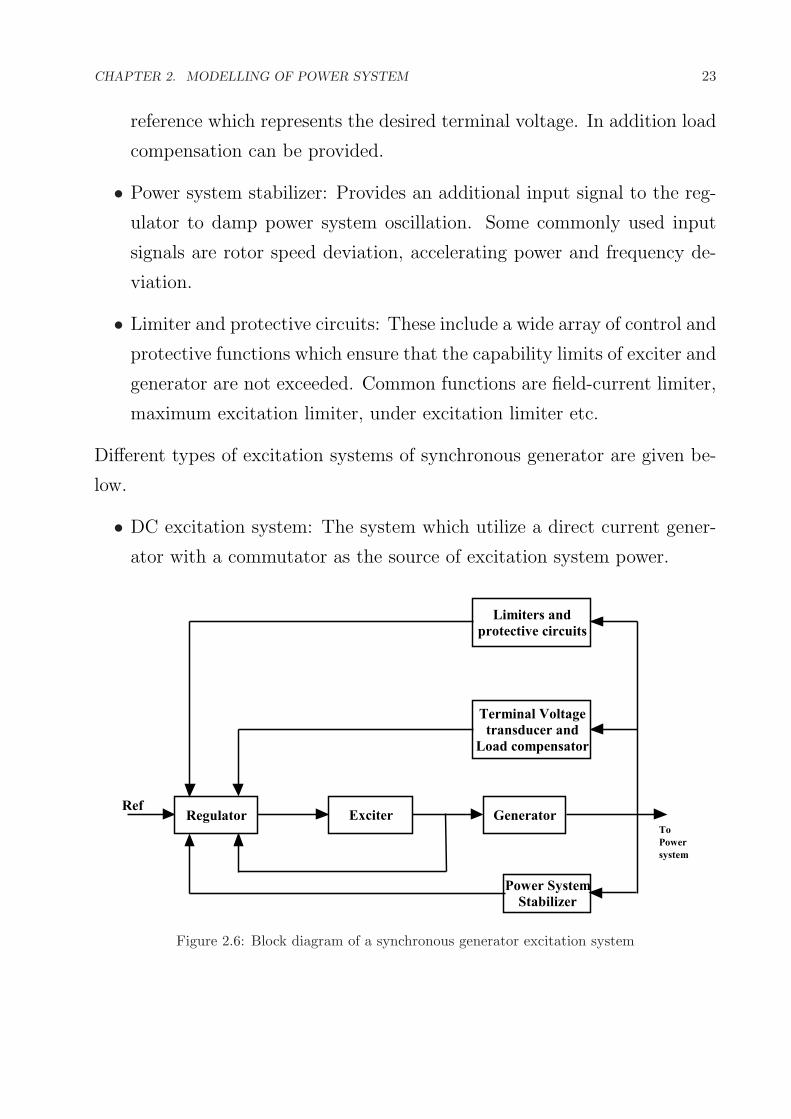
The functional block diagram of a typical control system for a large syn-
chronous generator is shown in Figure 2.6. The following is a brief introduc-
tion of the various subsystems identified in the above Figure 2.6.
• Exciter: Provides dc power to the synchronous machine field winding,
constituting the power angle of the excitation system.
• Regulator: processes and amplifies input control signal to a level and
form appropriate for control of the exciter.
• Terminal voltage transducer and load compensator: senses generator
terminal voltage, rectifies filters it to the dc quantity, compares it with a
CHAPTER 2. MODELLING OF POWER SYSTEM 23
reference which represents the desired terminal voltage. In addition load
compensation can be provided.
• Power system stabilizer: Provides an additional input signal to the reg-
ulator to damp power system oscillation. Some commonly used input
signals are rotor speed deviation, accelerating power and frequency de-
viation.
• Limiter and protective circuits: These include a wide array of control and
protective functions which ensure that the capability limits of exciter and
generator are not exceeded. Common functions are field-current limiter,
maximum excitation limiter, under excitation limiter etc.
Different types of excitation systems of synchronous generator are given be-
low.
• DC excitation system: The system which utilize a direct current gener-
ator with a commutator as the source of excitation system power.
Limiters and
protective circuits
Terminal Voltage
transducer and
Load compensator
Generator
Power System
Stabilizer
ExciterRegulatorTo
Power
system
Ref
Figure 2.6: Block diagram of a synchronous generator excitation system

CHAPTER 2. MODELLING OF POWER SYSTEM 24
• AC excitation system: The system which uses an alternator and either
stationary or rotating rectifiers to produce direct current needed for gen-
erator field.
• ST excitation system: The system in which excitation power is supplied
through transformers and rectifiers.
The first two types of exciters are also called rotating exciters which are
mounted on the same shaft as the generator and driven by the prime mover.
The voltage regulator for DC excitation systems were based on rotating am-
plifier (amplidyne) or magnetic amplifiers. AC and static excitation systems
invariably use electronic regulators which are fast acting and result in the
phase control of the controlled rectifiers using thyristors. Static excitation
system offers the ultimate response, which is virtually negligible, and ceiling
voltage which are limited only by generator rotor design considerations. With
the help of fast transient forcing of excitation and the boost of internal ma-
chine flux, the electrical output of the machine may be increased during the
first swing compared to the results obtainable with a slow exciter. The static
excitation system utilizes transformers to transform voltage to an appropri-
ate level. Rectifiers, either controlled or non-controlled, provide the necessary
direct current for generator field. The simplified model of a thyristor (static)
1
1 RsT
tV
cV
refV
1
A
A
K
sT
FMAXE
FMINE
fdE
Figure 2.7: Block diagram of thyristor excitation system with AVR
excitation system is shown in Figure 2.7. A high exciter gain, without tran-
sient gain reduction or derivative feedback is used. Parameter TR represents
CHAPTER 2. MODELLING OF POWER SYSTEM 25
the terminal voltage transducer time constant. The only nonlinearity associ-
ated with this model is that due to the ceiling on the exciter output voltage
represented by EFMAX and EFMIN . Due to small disturbances these limits
are ignored so that Efd is always within the limits and in Laplace domain
can be given as
Efd =KA
1 + sTA(Vref − Vc) (2.40)
Assuming that Vref is constant during a short period after application of
disturbance and by linearising equation (2.40), deviation of Efd with respect
to the steady state value is obtained as
∆Efd =KA
1 + sTA(−∆Vc) (2.41)
In the time domain the equation (2.41) can be written as
d
dt∆Efd = −KA
TA∆Vc − 1
TA∆Efd (2.42)
From Figure 2.7 we can write that
∆Vc =1
1 + sTA∆Vt (2.43)
In the time domain equation (2.43) can be written as
d
dt∆Vc =
1
TR(∆Vt −∆Vc) (2.44)
In order to obtain the state-space representation of the system, the state
vector should be redefined. Equations (2.42) and (2.44) introduce two new
state variables, namely ∆Vc and ∆Efd. However ∆Vt is not a state variable
and should be expressed in terms of other state variables. So we can write
that
∆Vt = K5∆δ + K6∆ψfd (2.45)
where
K5 =ed0
Vt0[−Ram1 + L1n1 + Laqsn1]+
eq0
Vt0[−Ran1 − L1m1 − Ladsm1] (2.46)
CHAPTER 2. MODELLING OF POWER SYSTEM 26
K6 =ed0
Vt0[−Ram2 + L1n2 + Laqsn2]+
eq0
Vt0
[−Ran2 − L1m2 + L
′ads
(1
Lfd−m2
)]
(2.47)
where ed0 and eq0 can be calculated as
ed0 = REid0 −XEiq0 + EB sin δ0 (2.48)
eq0 = REiq0 + XEid0 + EB cos δ0 (2.49)
id0 and iq0 can be obtained from equations (2.27) and (2.28). From the
previous expressions the state-space representation of the system is given by
d
dt
∆ωr
∆δ
∆ψfd
∆Vc
∆Efd
=
a11 a12 a13 0 0
a21 0 0 0 0
0 a32 a33 0 a35
0 a42 a43 a44 0
0 0 0 a54 a55
∆ωr
∆δ
∆ψfd
∆Vc
∆Efd
+
b1
0
0
0
0
∆Tm (2.50)
where
a35 = b32 =ω0Rfd
Ladu(2.51)
a42 =K5
TR(2.52)
a43 =K6
TR(2.53)
a44 = − 1
TR(2.54)
a54 = −KA
TA(2.55)
a55 = − 1
TA(2.56)

CHAPTER 2. MODELLING OF POWER SYSTEM 27
b1 = b11 =1
2H(2.57)
refV
1
1 RsT
1
A
A
K
sTV
cV
fdE3
31
K
sT 2K
eT
mT
1eT
2eT 1
2D
Hs K
r
0
s
1K
5KtV
6K
4K
Figure 2.8: Block diagram representation with excitation and AVR
Laplace transformation of equation (2.8) gives
∆ωr =1
2Hs + KD(∆Tm −∆Te) (2.58)
The variation of ψfd is determined by the field circuit dynamic equation,
which is given by equation (2.50) as
d
dt∆ψfd = a32∆δ + a33∆ψfd + a35∆Efd (2.59)
Laplace transform of equation (2.59) gives
∆ψfd =K3
1 + sT3[∆Efd −K4∆δ] (2.60)
where
K3 = −a35
a33(2.61)
K4 = −a32
a35(2.62)

CHAPTER 2. MODELLING OF POWER SYSTEM 28
T3 = − 1
a33(2.63)
Using equations (2.58), (2.60), (2.45), (2.22) and using Figure 2.7 the
block diagram representation of the system including excitation system can
be derived and is shown in Figure 2.8. So far the equations derived the
constants K2, K3 and K4 are usually positive. As long as K4 is positive,
the effect of field flux variation due to armature reaction is to introduce a
positive damping torque component. However there can be situation where
K4 is negative. K4 is negative where a hydraulic generator without damper
windings is operating at light load and is connected by a line of relatively
high resistance to reactance ratio to a large system.
Also K4 can be negative when a machine is connected to a large local
load, supplied partly by the generator and partly by the remote large system.
Under such conditions, the torques produced by induced currents in the field
due to armature reaction has components out of phase with ∆ω and produce
negative damping.
The coefficient K6 is always positive, whereas K5 can either be positive
or negative, depending on the operating condition and the external network
impedance RE + jXE. The value of K5 has a significant bearing on the
influence of the AVR on the damping of system oscillations. With K5 positive,
the effect of the AVR is to introduce a negative synchronizing torque and a
positive damping torque component. The constant K5 is positive for low
values of external system reactance and low generator outputs.
The reduction in Ks due to AVR action in such cases is usually of no
particular concern, because K1 is so high that the net Ks is significantly
greater than zero.
With K5 negative, the AVR action introduces a positive synchronizing
torque component and a negative damping torque component. This effect is
more pronounced as the exciter response increases.
For high values of external system reactance and high generator outputs

CHAPTER 2. MODELLING OF POWER SYSTEM 29
K5 is negative. In practice, the situation where K5 is negative are commonly
encountered. For such cases, a high response exciter is beneficial in increasing
synchronizing torque. However, in doing so, it introduces negative damping.
We thus have conflicting requirement with regard to exciter response. One
possible resource is to strike a compromise and set the exciter response so
that it results in sufficient synchronizing and damping torque components for
the expected range of the system operating conditions. This may not always
be possible. It may be necessary to use a high response exciter to provide
the required synchronizing toque and system stability performance. With a
very high external system reactance, even with low exciter response the net
damping torque coefficient may be negative.
With electrical power systems, the change in electrical torque of a syn-
chronous machine, following a small disturbance can be resolved into 2 com-
ponents.
∆Te = Ks∆δ + KD∆ω
Where Ks∆δ, the component of torque change is in phase with the rotor
angle perturbation ∆δ or called as synchronizing torque component.
KD∆ω, the component of torque change is in phase with the speed devi-
ation ∆ω or called as damping torque component.
System stability depends on the existence of both components of torque.
• Lack of sufficient synchronizing torque results in instability through a
periodic drift in rotor angle.
• Lack of sufficient damping torque results in oscillatory instability.
For a generator connected radially to a large power system, in the absence
of automatic voltage regulator (i.e. with constant field voltage), the insta-
bility is due to the lack of sufficient synchronizing torque (i.e. -ve Ks). This
results in instability through a non-oscillatory mode. For +ve values of Ks,
the synchronizing torque component opposes changes in the rotor angle from
the equilibrium point (i.e. an increase in the rotor angle will lead to a net
CHAPTER 2. MODELLING OF POWER SYSTEM 30
decelerating torque, until the rotor angle is restored to its equilibrium point
(∆δ = 0)). Similarly for +ve values of KD the damping torque component
opposes changes in the rotor speed from the steady-state operating point.
For a generator connected radially to a large power system, in the presence
of automatic voltage regulator, the instability is due to the lack of sufficient
damping torque. This results in instability through an oscillatory mode. A
number of factors can influence the damping coefficient of a synchronous
generator; including the generator’s design, the strength of the machine’s
interconnection to the grid and the setting of the excitation system. With
-ve damping torque causes the electromechanical oscillations to grow and
eventually causing loss of synchronism. This form of instability is normally
referred to as dynamic, small-signal or oscillatory instability to differentiate
it from the steady-state stability and transient stability.
For a generator connected radially to a large power system, in the presence
of automatic voltage regulator, the instability is due to the lack of sufficient
damping torque (i.e. -ve KD). This results in instability through an oscilla-
tory mode. A number of factors can influence the damping coefficient of a
synchronous generator including the generator’s design, the strength of the
machine’s interconnection to the grid and the setting of the excitation sys-
tem. With -ve damping torque (i.e. -ve KD) causes the electromechanical
oscillations to grow and eventually causing loss of synchronism. This form
of instability is normally referred to as dynamic, small-signal or oscillatory
instability to differentiate it from the steady-state stability and transient sta-
bility.
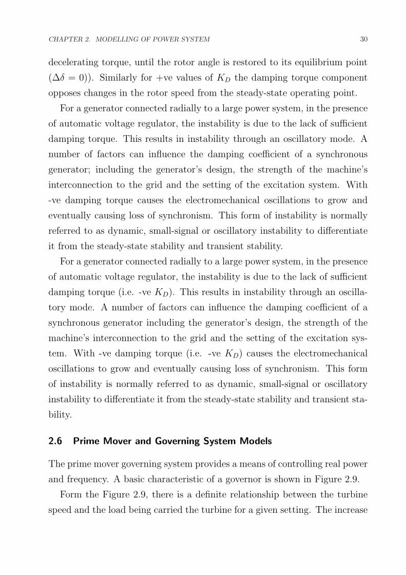
2.6 Prime Mover and Governing System Models
The prime mover governing system provides a means of controlling real power
and frequency. A basic characteristic of a governor is shown in Figure 2.9.
Form the Figure 2.9, there is a definite relationship between the turbine
speed and the load being carried the turbine for a given setting. The increase

CHAPTER 2. MODELLING OF POWER SYSTEM 31
Slope= -R
where R = speed regulation
LOAD PM
25% 50%
99%
98%
SPEED
Figure 2.9: Governor Characteristic
in load will lead to a decrease in speed. The example given in Figure 2.9 shows
that if the initial operating is at and the load is dropped to 25 percent, the
speed will increase. In order to maintain the speed at , the governor setting
by changing the spring tension in the fly ball type of governor will be resorted
to and the characteristic of the governor will be indicated by the dotted line
as shown in Figure 2.9.
Figure 2.9 illustrates the ideal characteristic of the governor whereas the
actual characteristic departs from the ideal one due to valve openings at
different loadings. In contrast to the excitation system, the governing system
is a relatively slow response system because of the slow reaction of mechanic
operation of turbine machine.
In Figure 2.10, the schematic diagram of a speed governing system that
controls the real power flow in the power system is shown.
As shown, the speed governor is made up of the following parts:
• Speed governor: This is a fly ball type of speed governor. The mechanism
provides upward and downward vertical movements proportional to the

CHAPTER 2. MODELLING OF POWER SYSTEM 32
SpeedGovernor
Speed Changer
Lower
Raise
To governorcontrolledvalves
To open
To close
Hydraulicamplifier
Figure 2.10: Speed governing system
change in speed.
• Linkage mechanism: Provide a movement to the control valve in the
proportion to change in speed.
• Hydraulic amplifier: Low power level pilot valve movement is converted
into high power level piston valve movement which is necessary to open
or close the steam valve against high pressure steam.
• Speed Changer: Provides a steady-state power output setting for the
turbine.
When selecting a prime mover to model in a simulation, special consider-
ations are required as different types of turbine required different operating
conditions and hence the effects on the power system stability will be differ-
ent. Using an example of hydraulic turbines, a large transient (temporary)
droop with a long resettling time is needed for stable control performance
because of the ”water hammer” effect; a change in gate position generates
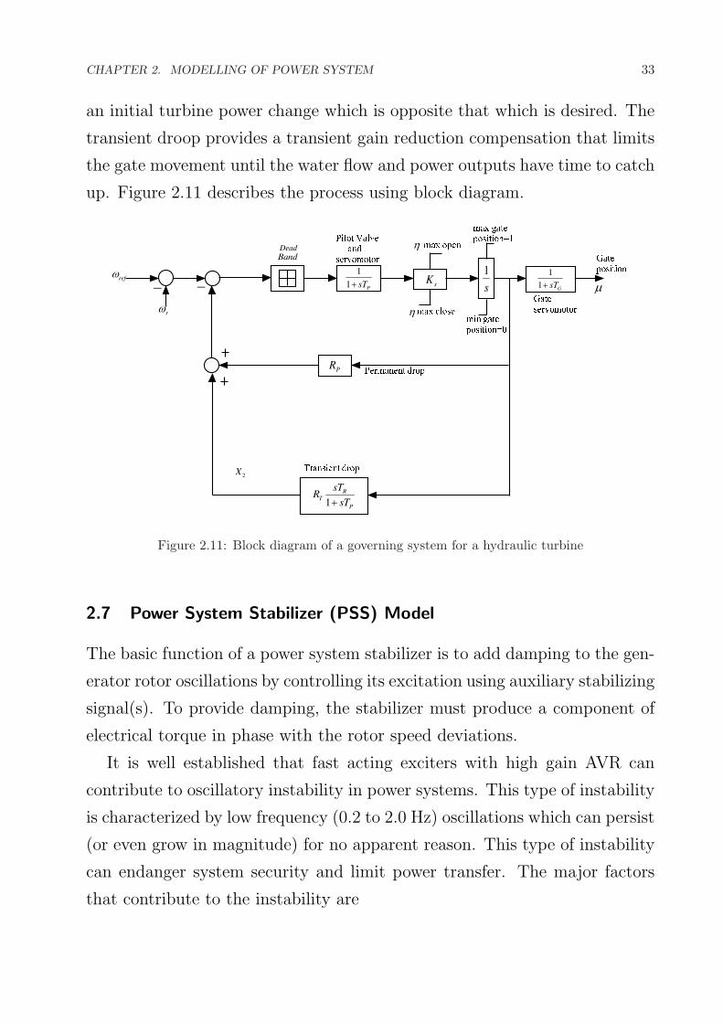
CHAPTER 2. MODELLING OF POWER SYSTEM 33
an initial turbine power change which is opposite that which is desired. The
transient droop provides a transient gain reduction compensation that limits
the gate movement until the water flow and power outputs have time to catch
up. Figure 2.11 describes the process using block diagram.
ref
r
Dead
Band
1
1G
sT
1
ssK1
1 PsT
PR
2X
1
RT
P
sTR
sT
Figure 2.11: Block diagram of a governing system for a hydraulic turbine
2.7 Power System Stabilizer (PSS) Model
The basic function of a power system stabilizer is to add damping to the gen-
erator rotor oscillations by controlling its excitation using auxiliary stabilizing
signal(s). To provide damping, the stabilizer must produce a component of
electrical torque in phase with the rotor speed deviations.
It is well established that fast acting exciters with high gain AVR can
contribute to oscillatory instability in power systems. This type of instability
is characterized by low frequency (0.2 to 2.0 Hz) oscillations which can persist
(or even grow in magnitude) for no apparent reason. This type of instability
can endanger system security and limit power transfer. The major factors
that contribute to the instability are

CHAPTER 2. MODELLING OF POWER SYSTEM 34
• Loading of the generator or tie line
• Power transfer capability of transmission lines
• Power factor of the generator (leading power factor operation is more
problematic than lagging power factor operation)
• AVR gain
A cost efficient and satisfactory solution to the problem of oscillatory in-
stability is to provide damping for generator rotor oscillations. This is con-
veniently done by providing Power System Stabilizers (PSS) which are sup-
plementary controllers in the excitation systems. The objective of designing
PSS is to provide additional damping torque without affecting the synchro-
nizing torque at critical oscillation frequencies. It can be generally said that
need for PSS will be felt in situations when power has to be transmitted over
long distances with weak AC ties. Even when PSS may not be required under
normal operating conditions, they allow satisfactory operation under unusual
or abnormal conditions which may be encountered at times. Thus, PSS has
become a standard option with modern static exciters and it is essential for
power engineers to use these effectively. Retrofitting of existing excitation
systems with PSS may also be required to improve system stability.
The theoretical basis for a PSS may be illustrated with the aid of the block
diagram shown in Figure 2.12. This is an extension of the block diagram
shown in Figure 2.8 and includes the effects of a PSS. Since the purpose of a
PSS is to introduce a damping torque component, a logical signal to use for
controlling generator excitation is the speed deviation ∆ωr.
If the exciter transfer function and the generator transfer function be-
tween ∆Efd and ∆Te were pure gains, a direct feedback of ∆ωr would result
in a damping torque component. However, in practice both the generator
and the exciter exhibit frequency dependent gain and phase characteristics.
Therefore, the PSS transfer function Gpss(s) should have appropriate phase
compensation circuits to compensate for the phase lag between the exciter

CHAPTER 2. MODELLING OF POWER SYSTEM 35
refV
sV
( )pssG s
1
1R
sT
1
A
A
K
sTV
cV
fdE3
31
K
sT 2K
eT
mT
1eT
2eT 1
2 DHs K
r
0
s
1K
5KtV
6K
4K
Figure 2.12: Block diagram of thyristor excitation system with AVR and PSS
input and the electrical torque. In the ideal case, with the phase charac-
teristic of Gpss(s) being an exact inverse of the exciter and generator phase
characteristics to be compensated, the PSS would result in a pure damping
torque at all oscillating frequencies.
Figure 2.12 shows the block diagram of the excitation system, including
the AVR and PSS. The PSS representation in Figure 2.13 consists of three
blocks: a phase compensation block, a signal washout block, and a gain block.
The phase compensation block provides the appropriate phase lead char-
acteristic to compensate for the phase lag between the exciter input and the
generator electrical (air-gap) torque. The figure shows a single first-order
block. In practice, two or more first-order blocks may be used to achieve
the desired phase compensation. In some cases, second-order blocks with
complex roots have been used.
Normally, the frequency range of interest is 0.1 to 2.0 Hz and the phase-
lead network should provide compensation over this entire frequency range.
The phase characteristic to be compensated changes with system conditions;
therefore a compromise is made and a characteristic is acceptable for dif-
ferent system conditions is selected. Generally some under compensation is

CHAPTER 2. MODELLING OF POWER SYSTEM 36
Gain
Terminal
Voltage
Transducer
Phase
Compensation
Signal
washout
Exciter &AVR
Figure 2.13: Block diagram of thyristor excitation system with AVR and PSS
desirable so that the PSS, in addition to significantly increase the damping
torque, results in a slight increase of the synchronizing torque.
The signal washout block serves as a high-pass filter, with the time con-
stant Tw high enough to allow signals associated with oscillations in ωr to
pass unchanged. Without it, steady changes in speed would modify the ter-
minal voltage. It allows the PSS to respond only to changes in speed. From
the view point of the washout function, the value of Tw is not critical and
may be in the range of 1 to 20 seconds. The main consideration is that
it be long enough to pass stabilizing signals at the frequencies of interest
unchanged, but not so long that it leads to undesirable generator voltage
excursions during system-islanding conditions.
The stabilizer gain determines the amount of damping introduced by the
PSS. Ideally, the gain should be set at a value corresponding to maximum
damping; however it is often limited by other considerations.
From Figure 2.13, using perturbed values, we have
∆v2 =pTw
1 + pTw(KSTAB∆ωr) (2.64)
Hence
p∆v2 = KSTABp∆ωr − 1
Tw∆v2 (2.65)
Substituting for p∆ωr by equation (2.31), we obtain the expression for
p∆v2 in terms of the state variables.

CHAPTER 2. MODELLING OF POWER SYSTEM 37
p∆v2 = KSTAB
[a11∆ωr + a12∆δ + a13∆ψfd +
1
2H∆Tm
]− 1
Tw∆v2
= a51∆ωr + a52∆δ + a53∆ψfd + a55∆v2 +KSTAB
2H∆Tm (2.66)
where
a51 = KSTABa11 (2.67)
a52 = KSTABa12 (2.68)
a53 = KSTABa13 (2.69)
a55 = − 1
Tw(2.70)
Since p∆v2 is not a function of ∆vc and ∆v3, a54 = a56 = 0
∆vs = ∆v2
(1 + pT1
1 + pT2
)(2.71)
Hence
p∆vs =T1
T2p∆v2 +
1
T2∆v2 − 1
T2∆vs (2.72)
Substitution for p∆v2, given by equation (2.66), yields
p∆vs = a61∆ωr+a62∆δ+a63∆ψfd+a64∆vc+a65∆v2+a66∆vs+T1
T2
KSTAB
2H∆Tm
(2.73)
where
a61 =T1
T2a51 (2.74)
a62 =T1
T2a52 (2.75)
CHAPTER 2. MODELLING OF POWER SYSTEM 38
a63 =T1
T3a53 (2.76)
a65 =T1
T2a55 +
1
T2(2.77)
a66 = − 1
T2(2.78)
From Figure 2.12 we have
∆Efd = KA(∆vs −∆vc) (2.79)
The field circuit equation, with PSS included becomes
p∆ψfd = a32∆δ + a33∆ψfd + a34∆vc + a36∆vs (2.80)
where
a36 =ω0Rfd
LaduKA (2.81)
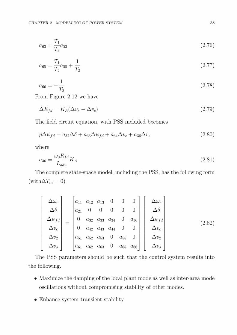
The complete state-space model, including the PSS, has the following form
(with∆Tm = 0)
∆ωr
∆δ
∆ψfd
∆vc
∆v2
∆vs
=
a11 a12 a13 0 0 0
a21 0 0 0 0 0
0 a32 a33 a34 0 a36
0 a42 a43 a44 0 0
a51 a52 a53 0 a55 0
a61 a62 a63 0 a65 a66
∆ωr
∆δ
∆ψfd
∆vc
∆v2
∆vs
(2.82)
The PSS parameters should be such that the control system results into
the following.
• Maximize the damping of the local plant mode as well as inter-area mode
oscillations without compromising stability of other modes.
• Enhance system transient stability

CHAPTER 2. MODELLING OF POWER SYSTEM 39
• Not adversely affect system performance during major system upsets
which cause large frequency excursions
• Minimize the consequences of excitation system malfunction due to com-
ponent failure.

Chapter 3
CONVENTIONAL POWER SYSTEM
STABILIZERS
3.1 Introduction
In this chapter, a conventional power system stabilizer is designed on the ba-
sis of the block diagram representation of the system introduced in chapter
2. Here the design procedure is performed in the frequency domain. Conven-
tional power system stabilizers (CPSSs) are basically designed on the basis
of a linear model for the power system. The power system is first linearised
around a specific operating point of the system. Then, assuming that dis-
turbances are small such that the linear model remains valid, the CPSS is
designed. Therefore, a CPSS is most useful for preserving dynamic stability
of the power system.
3.2 Conventional Power System Stabilizer Design
The basic function of a PSS is to add damping to the generator rotor os-
cillations by controlling its excitation using auxiliary stabilizing signal. To
provide damping, the stabilizer must produce a component of electrical torque
in phase with the rotor speed deviation.
For the simplicity a conventional PSS is modelled by two stage (identical),
lead/lag network which is represented by a gain KSTAB and two time con-
40

CHAPTER 3. CONVENTIONAL POWER SYSTEM STABILIZERS 41
stants T1 and T2. This network is connected with a washout circuit of a time
constant Tw as shown in Figure 3.1.
rSTAB
K1
w
w
sT
sT
1
2
1
1
sT
sT
2v
sV
Figure 3.1: Block diagram of PSS
In Figure 3.1 the phase compensation block provides the appropriate phase
lead characteristics to compensate for the phase lag between exciter input
and generator electrical torque. The phase compensation may be a single
first order block as shown in Figure 3.1 or having two or more first order
blocks or second order blocks with complex roots.
governor
generator
PSS
AVR
exciter
Transmission
Line Infinite
Bus
Turbine
Vt
Vref
Pm
Figure 3.2: Power System Configuration

CHAPTER 3. CONVENTIONAL POWER SYSTEM STABILIZERS 42
The signal washout block serves as high pass filter, with time constant
Tw high enough to allow signals associated with oscillations in ωr to pass
unchanged, which removes d.c. signals. Without it, steady changes in speed
would modify the terminal voltage. It allows PSS to respond only to changes
in speed.
The stabilizer gain KSTAB determines the amount of damping introduced
by PSS. Ideally, the gain should be set at a value corresponding to maximum
damping; however, it is limited by other consideration.
The block diagram of a single machine infinite bus (SMIB) system, which
illustrates the position of a PSS, is shown in Figure 3.2.
The system consists of a generating unit connected to an infinite bus
through a transformer and a pair of transmission lines. An excitation system
and automatic voltage regulator (AVR) are used to control the terminal volt-
age of the generator. An associated governor monitors the shaft frequency
and controls mechanical power.
Adding a PSS to the block diagram shown in Figure 2.8, the block diagram
of the power system with PSS is obtained as shown in Figure 3.3. Since the
refV
sV
( )pssG s
1
1R
sT
1
A
A
K
sTV
cV
fdE3
31
K
sT 2K
eT
mT
1eT
2eT 1
2 DHs K
r
0
s
1K
5KtV
6K
4K
Figure 3.3: Block diagram of a linear model of a synchronous machine with a PSS
purpose of a PSS is to introduce a damping torque component, a logical signal

CHAPTER 3. CONVENTIONAL POWER SYSTEM STABILIZERS 43
to use as the input of PSS is ∆ωr. If the exciter transfer function and the
generator transfer function between ∆Efd and ∆Te were pure gains, a direct
feedback of ∆ωr would result in a damping torque component. However, both
transfer functions between ∆Efd and ∆Te exhibit frequency dependent gain
and phase characteristics. Therefore, the CPSS transfer function should have
an appropriate phase compensation circuit to compensate for the phase lag
between the exciter input and the electrical torque. In the ideal case, with
the phase characteristics of Gpss(s) being an exact inverse of the exciter and
generator phase characteristics, the CPSS would result in a pure damping
torque at all oscillating frequencies.
1( )G s
2( )G S
2( )H s 1
( )H s
( )p
G s
refV
r
Figure 3.4: Simplified block diagram to design a CPSS
The block diagram of Figure 3.3 can be reduced to the block diagram
shown in Figure 3.4, where
G1(s) =KAK3
TAT3s2 + (TAT3)s + 1(3.1)
G2(s) =K2K3s
2 + K2s
2HT3s2 + (2H + KdT3)s2 + (K1T3ω0 + Kd)s + ω0(K1 −K2K3K4)
(3.2)

CHAPTER 3. CONVENTIONAL POWER SYSTEM STABILIZERS 44
H1(s) =−2K6Hs2 −K6Kds + ω0(K2K5 −K1K6)
K2s(3.3)
H2(s) =1
1 + sTR(3.4)
( )p
G s
refV
r( )G s
Figure 3.5: Compact block diagram to design a CPSS
The block diagram in Figure 3.4 can be simplified to the block diagram
shown in Figure 3.5.
G(s) =G1(s)G2(s)
1 + G1(s)G2(s)H1(s)H2(s)(3.5)
which is expanded to
G(s) =−KAK3(K3s + 1)
a6s6 + a5s5 + a4s4 + a3s3 + a2s2 + a1s + a0(3.6)
where
a6 = 2TATRT 23 H (3.7)
a5 = T3[2KAT3H + KATR(2H + KdT3) + 2TRH(TA + T3)] (3.8)
a4 = (2H+KdT3)[KAT3+TR(TA+T3)]+2T3H(TA+T3+TR)+TAT3TR(K1T3ω0+Kd)
(3.9)
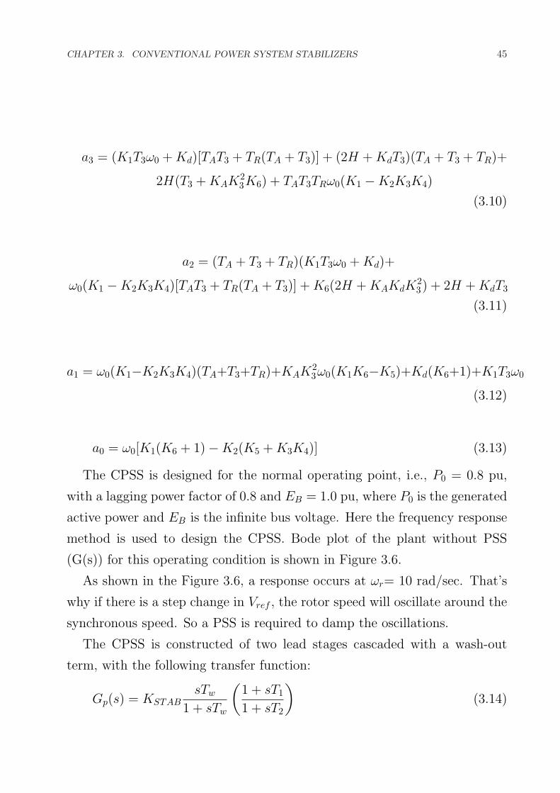
CHAPTER 3. CONVENTIONAL POWER SYSTEM STABILIZERS 45
a3 = (K1T3ω0 + Kd)[TAT3 + TR(TA + T3)] + (2H + KdT3)(TA + T3 + TR)+
2H(T3 + KAK23K6) + TAT3TRω0(K1 −K2K3K4)
(3.10)
a2 = (TA + T3 + TR)(K1T3ω0 + Kd)+
ω0(K1 −K2K3K4)[TAT3 + TR(TA + T3)] + K6(2H + KAKdK23) + 2H + KdT3
(3.11)
a1 = ω0(K1−K2K3K4)(TA+T3+TR)+KAK23ω0(K1K6−K5)+Kd(K6+1)+K1T3ω0
(3.12)
a0 = ω0[K1(K6 + 1)−K2(K5 + K3K4)] (3.13)
The CPSS is designed for the normal operating point, i.e., P0 = 0.8 pu,
with a lagging power factor of 0.8 and EB = 1.0 pu, where P0 is the generated
active power and EB is the infinite bus voltage. Here the frequency response
method is used to design the CPSS. Bode plot of the plant without PSS
(G(s)) for this operating condition is shown in Figure 3.6.
As shown in the Figure 3.6, a response occurs at ωr= 10 rad/sec. That’s
why if there is a step change in Vref , the rotor speed will oscillate around the
synchronous speed. So a PSS is required to damp the oscillations.
The CPSS is constructed of two lead stages cascaded with a wash-out
term, with the following transfer function:
Gp(s) = KSTABsTw
1 + sTw
(1 + sT1
1 + sT2
)(3.14)
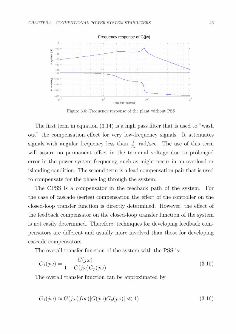
CHAPTER 3. CONVENTIONAL POWER SYSTEM STABILIZERS 46
−100
−80
−60
−40
−20
0
Mag
nitu
de (
dB)
10−1
100
101
102
−450
−360
−270
−180
−90
Pha
se (
deg)
Frequency response of G(jw)
Frequency (rad/sec)
Figure 3.6: Frequency response of the plant without PSS
The first term in equation (3.14) is a high pass filter that is used to ”wash
out” the compensation effect for very low-frequency signals. It attenuates
signals with angular frequency less than 1Tw
rad/sec. The use of this term
will assure no permanent offset in the terminal voltage due to prolonged
error in the power system frequency, such as might occur in an overload or
islanding condition. The second term is a lead compensation pair that is used
to compensate for the phase lag through the system.
The CPSS is a compensator in the feedback path of the system. For
the case of cascade (series) compensation the effect of the controller on the
closed-loop transfer function is directly determined. However, the effect of
the feedback compensator on the closed-loop transfer function of the system
is not easily determined. Therefore, techniques for developing feedback com-
pensators are different and usually more involved than those for developing
cascade compensators.
The overall transfer function of the system with the PSS is:
G1(jω) =G(jω)
1−G(jω)Gp(jω)(3.15)
The overall transfer function can be approximated by
G1(jω) ≈ G(jω)for(|G(jω)Gp(jω)| ¿ 1) (3.16)

CHAPTER 3. CONVENTIONAL POWER SYSTEM STABILIZERS 47
and
G1(jω) ≈ 1
Gp(jω)for(|G(jω)Gp(jω)| À 1) (3.17)
The condition when |G(jω)Gp(jω)| ≈ 1 is still undefined, in which case
neither equation (3.16) nor equation (3.17) is applicable. In the design proce-
dure, this condition is neglected. The aforementioned approximations allow
investigation of the qualitative results to be obtained. After the design of
Gp(s) is completed, the closed-loop frequency response of the whole system
will be obtained and the designer will make sure that the stabilizer perfor-
mance is satisfactory in the frequency design of interest.
Thus, Gp(s) should be designed such that:
• |G(jω)Gp(jω)| À 1 in the vicinity of the resonance region of the sys-
tem. This means that the overall transfer function of the system will be
approximately equal to − 1Gp(jω) in the resonance region of the system.
Therefore, gain and phase responses of − 1Gp(jω) should be desirable in
that region.
• 1|Gp(jω)| is considerably less than |G(jω)| in that region.
• Phase of G(jω)Gp(jω) is approximately equal to -180 degrees in that
region. This means that the output of Gp(s) will have an opposite phase
with respect to the input to G(s) causing a negative feedback (notice
positive signs of the comparator inputs in Figure 3.4). For this to happen,
Gp(s) must be a lead compensator.
Taking the above situations into consideration, the CPSS is designed. The
designed values are KSTAB= 20, Tw=1.4 sec, T1=0.154 sec, T2=0.033 sec.
Figure 3.7 shows the frequency response of the CPSS.
Figure 3.8 shows the log magnitude of 1�Gp(jω) placed over log magnitude
of G(jω).

CHAPTER 3. CONVENTIONAL POWER SYSTEM STABILIZERS 48
20
30
40
50
60
Mag
nitu
de (
dB)
10−1
100
101
102
0
45
90
135
Pha
se (
deg)
frequency response of the CPSS
Frequency (rad/sec)
Figure 3.7: Frequency response of the CPSS (Gp(jω))
−100
−80
−60
−40
−20
0
Mag
nitu
de (
dB)
10−1
100
101
102
−450
−360
−270
−180
−90
0
Pha
se (
deg)
frequency response of G(jw) and l/Gp(jw)
Frequency (rad/sec)
Figure 3.8: Frequency response of log magnitude of G(jω) and 1�Gp(jω)
By applying the designed Gp(s) to the system, the closed loop frequency
response will be obtained as Figure 3.9.
From Figure 3.9 it shows that the sharp resonance which was observed
in Figure 3.6 is made smooth with a smaller magnitude and it occurs at a
smaller frequency.
3.3 Conclusion
The Conventional power system stabilizer (CPSS) damps the low frequency
oscillations in the shaft speed of a synchronous machine. Since the design
is on the basis of a block diagram of the system derived for a specific op-

CHAPTER 3. CONVENTIONAL POWER SYSTEM STABILIZERS 49
−100
−80
−60
−40
−20
Mag
nitu
de (
dB)
10−1
100
101
102
−450
−360
−270
−180
−90
Pha
se (
deg)
closed loop frequency response
Frequency (rad/sec)
Figure 3.9: Closed loop frequency response of the system with CPSS
erating point, the CPSS has the best response for this operating point. If
the operating point of the system changes, the performance of the CPSS will
degrade.

Chapter 4
DESIGN OF FUZZY LOGIC BASED
PSS
4.1 Introduction
In 1965, Lofty A. Zadeh of the University of California at Berkeley published
”Fuzzy Sets” which laid out the mathematics of fuzzy set theory and, by
extension, fuzzy logic. Zadeh had observed that conventional computer logic
couldn’t manipulate data that represented subjective or vague ideas, so he
created fuzzy logic to allow computers to determine the distinctions among
data with shades of gray, similar to the process of human reasoning. Fuzzy
logic, as its name suggests, is the logic underlying modes of reasoning which
are approximate rather than exact.
FLCs are very useful when an exact mathematical model of the plant is
not available; however, experienced human operators are available for provid-
ing qualitative rules to control the system. Fuzzy logic, which is the logic on
which fuzzy logic control is based, is much closer in spirit to human thinking
and natural language than the traditional logic systems. Basically, it provides
an effective mean of capturing the approximate, inexact nature of our knowl-
edge about the real world. Viewed in this perspective, the essential part of
the fuzzy logic controller (FLC) is a set of linguistic control rules related by
dual concepts of fuzzy implication and the compositional rule of inference.
50

CHAPTER 4. DESIGN OF FUZZY LOGIC BASED PSS 51
In essence, the FLC provides an algorithm which can convert the linguistic
control strategy based on expert knowledge into an automatic control strat-
egy. The methodology of the FLC appears very useful when the processes
are too complex for analysis by conventional quantitative techniques.
Fuzzy logic is a derivative from classical Boolean logic and implements
soft linguistic variables on a continuous range of truth values to be defined
between conventional binary i.e. [0, 1]. It can often be considered a subset
of conventional set theory. The fuzzy logic is capable to handle approximate
information in a systematic way and therefore it is suited for controlling non-
linear systems and for modeling complex systems where an inexact model
exists or systems where ambiguity or vagueness is common.
The importance of fuzzy logic derives from the fact that most modes of
human reasoning and especially common sense reasoning are approximate in
nature. In doing so, the fuzzy logic approach allows the designer to han-
dle efficiently very complex closed-loop control problems. There are many
artificial intelligence techniques that have been employed in modern power
systems, but fuzzy logic has emerged as the powerful tool for solving chal-
lenging problems. As compared to the conventional PSS, the Fuzzy Logic
Controller (FLC) has some advantages such as:
• A simpler and faster methodology.
• It does not need any exact system mathematical model.
• It can handle nonlinearity of arbitrary complexity.
• It is based on the linguistic rules with an IF-THEN general structure,
which is the basis of human logic.
• It is more robust than conventional nonlinear controllers.

CHAPTER 4. DESIGN OF FUZZY LOGIC BASED PSS 52
4.2 Fuzzy sets
Fuzzy set, as the name implies, is a set without a crisp boundary. The
transition from ”belong to a set” to ”not belong to a set” is gradual, and
this smooth transition is characterized by membership functions. The fuzzy
set theory is based on fuzzy logic, where a particular object has a degree
of membership in a given set that may be anywhere in the range of 0 to 1.
On the other hand, classical set theory is based on Boolean logic, where a
particular object or variable is either a member of a given set (logic 1), or it
is not (logic 0).
4.3 Membership functions
A membership function is a curve that defines how the values of a fuzzy
variable in a certain region are mapped to a membership value µ (or degree
of membership) between 0 and 1. The MF maps each element of X to a
membership degree between 0 and 1 (included). Obviously, the definition of
a fuzzy set is a simple extension of the definition of a classical (crisp) set in
which the characteristic function is permitted to have any value between 0
and 1. If the value of the membership function is restricted to either 0 or 1,
then A is reduced to a classical set. For clarity, we shall also refer to classical
sets as ordinary sets, crisp sets, non-fuzzy sets, or just sets. Usually, X is
referred to as the universe of discourse, or simply the universe, and it may
consist of discrete (ordered or non-ordered) objects or it can be a continuous
space. In practice, when the universe of discourse X is a continuous space,
we usually partition it into several fuzzy sets whose MFs cover X in a more
or less uniform manner. These fuzzy sets, which usually carry names that
conform to adjectives appearing in our daily linguistic usage, such as ”large,”
”medium,” or ”small,” are called linguistic values or linguistic labels. Thus,
the universe of discourse X is often called the linguistic variable. The fuzzy
membership not only provides for a meaningful and powerful representation

CHAPTER 4. DESIGN OF FUZZY LOGIC BASED PSS 53
of measurement of uncertainties, but also provides the meaningful represen-
tation of vague concepts expressed in natural language. If X is a collection
of objects denoted generically by x, then a fuzzy set in X is defined as a set
of ordered pairs.
A = {(x, µA(x))/xεX} (4.1)
where µA(x) is called the membership function for the set A. There exist
different shapes of membership functions. The shapes could be triangular,
trapezoidal, curved or their variations.
The various types of membership functions are given below.
4.3.1 Triangular Membership Function
A triangular membership function is specified by three parameters {a, b, c}as follows:
f(x; a, b, c) =
0, x ≤ ax−ab−a , a ≤ x ≤ bc−xc−b , b ≤ x ≤ c
0, c ≤ x
(4.2)
The parameters a and c locate the feet of the triangle and the parameter b
0 1 2 3 4 5 6 7 8 9 100
0.2
0.4
0.6
0.8
1
trimf, P=[3 6 8]
Mem
bers
hip
Gra
des
Figure 4.1: Triangular Membership Function
locate the peak.
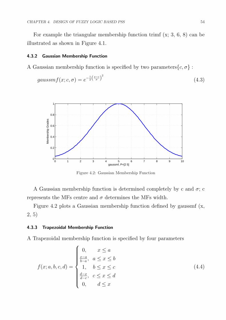
CHAPTER 4. DESIGN OF FUZZY LOGIC BASED PSS 54
For example the triangular membership function trimf (x; 3, 6, 8) can be
illustrated as shown in Figure 4.1.
4.3.2 Gaussian Membership Function
A Gaussian membership function is specified by two parameters{c, σ} :
gaussmf(x; c, σ) = e−12(
x−cσ )
2
(4.3)
0 1 2 3 4 5 6 7 8 9 100
0.2
0.4
0.6
0.8
1
gaussmf, P=[2 5]
Mem
bers
hip
Gra
des
Figure 4.2: Gaussian Membership Function
A Gaussian membership function is determined completely by c and σ; c
represents the MFs centre and σ determines the MFs width.
Figure 4.2 plots a Gaussian membership function defined by gaussmf (x,
2, 5)
4.3.3 Trapezoidal Membership Function
A Trapezoidal membership function is specified by four parameters
f(x; a, b, c, d) =
0, x ≤ ax−ab−a , a ≤ x ≤ b
1, b ≤ x ≤ cd−xd−c , c ≤ x ≤ d
0, d ≤ x
(4.4)
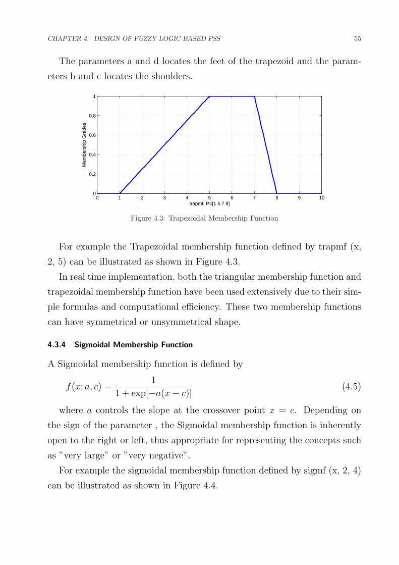
CHAPTER 4. DESIGN OF FUZZY LOGIC BASED PSS 55
The parameters a and d locates the feet of the trapezoid and the param-
eters b and c locates the shoulders.
0 1 2 3 4 5 6 7 8 9 100
0.2
0.4
0.6
0.8
1
trapmf, P=[1 5 7 8]
Mem
bers
hip
Gra
des
Figure 4.3: Trapezoidal Membership Function
For example the Trapezoidal membership function defined by trapmf (x,
2, 5) can be illustrated as shown in Figure 4.3.
In real time implementation, both the triangular membership function and
trapezoidal membership function have been used extensively due to their sim-
ple formulas and computational efficiency. These two membership functions
can have symmetrical or unsymmetrical shape.
4.3.4 Sigmoidal Membership Function
A Sigmoidal membership function is defined by
f(x; a, c) =1
1 + exp[−a(x− c)](4.5)
where a controls the slope at the crossover point x = c. Depending on
the sign of the parameter , the Sigmoidal membership function is inherently
open to the right or left, thus appropriate for representing the concepts such
as ”very large” or ”very negative”.
For example the sigmoidal membership function defined by sigmf (x, 2, 4)
can be illustrated as shown in Figure 4.4.

CHAPTER 4. DESIGN OF FUZZY LOGIC BASED PSS 56
0 1 2 3 4 5 6 7 8 9 100
0.2
0.4
0.6
0.8
1
sigmf, P=[2 4]
Mem
bers
hip
Gra
des
Figure 4.4: Sigmoidal Membership Function
4.3.5 Generalized bell Membership Function
A generalized bell membership function is specified by three parameters (a,
b, c)
f(x; a, b, c) =1
1 +∣∣x−c
a
∣∣2b(4.6)
where the parameter b is usually positive. The parameter c locates the
centre of the curve. If b is negative, the slope of the membership function
becomes an upside-down bell.
0 1 2 3 4 5 6 7 8 9 100
0.2
0.4
0.6
0.8
1
gbellmf, P=[2 4 6]
Mem
bers
hip
Gra
des
Figure 4.5: Generalized bell Membership Function
For example the generalized bell membership function defined by gbellmf
(x, 2, 4, 6) can be illustrated as shown in Figure 4.5.

CHAPTER 4. DESIGN OF FUZZY LOGIC BASED PSS 57
4.4 Fuzzy Systems
The fuzzy inference system or fuzzy system is a popular computing frame-
work based on the concept of fuzzy set theory, fuzzy if-then rules, and fuzzy
reasoning.
Decision makinglogic
Fuzzificationinterface
Defuzzificationinterface
Controlled System (process)
Knowledge baseFuzzy Fuzzy
Control Signal(non-fuzzy)
OutputSignal
Figure 4.6: Block diagram of Fuzzy logic controller
The fuzzy inference system basically consists of a formulation of the map-
ping from a given input set to an output set using FL as shown in Figure 4.6.
The mapping process provides the basis from which the inference or conclu-
sion can be made. The basic structure of fuzzy inference system consists of
three conceptual components: a rule base, which contains a selection of fuzzy
rules; a data base, which defines the membership functions used in the fuzzy
rules; and a reasoning mechanism which performs the inference procedure
upon the rules and given facts to derive a reasonable output or conclusion.
The fuzzy logic controller comprises 4 principle components: fuzzification
interface, knowledge base, decision making logic, and defuzzification inter-
face.
• Fuzzification: In fuzzification, the values of input variables are measured
i.e. it converts the input data into suitable linguistic values.
• Knowledge base: The knowledge base consists of a database and linguis-

CHAPTER 4. DESIGN OF FUZZY LOGIC BASED PSS 58
tic control rule base. The database provides the necessary definitions,
which are used to define the linguistic control rules and fuzzy data ma-
nipulation in an FLC. The rule base characterizes the control policy of
domain experts by means of set of linguistic control rules.
• Decision making logic: The decision making logic has the capability of
stimulating human decision making based on fuzzy concepts.
• Defuzzification: The defuzzification performs scale mapping, which con-
verts the range of values of output variables into corresponding universe
of discourse. If the output from the defuzzifier is a control action for a
process, then the system is a non-fuzzy logic decision system. There are
different techniques for defuzzification such as maximum method, height
method, centroid method etc.
The basic inference process consists of the following five steps:
• Step 1: Fuzzification of input variables
• Step2: Application of fuzzy operator (AND, OR, NOT) in the IF (an-
tecedent) part of the rule
• Step3: Implication from the antecedent to the consequent THEN part
of the rule
• Step4: Aggregation of the consequents across the rules
• Step5: Defuzzification
4.5 Implication Methods
There are number of implication methods to fuzzy logic, but only two widely
used methods are discussed here. Those are Mamdani type fuzzy model and
Sugeno type fuzzy model.

CHAPTER 4. DESIGN OF FUZZY LOGIC BASED PSS 59
4.5.1 Mamdani Fuzzy Model
Mamdani fuzzy rule for a fuzzy controller involving three input variables and
two output variables can be described as follows:
IF x1 is A AND x2 is B AND x3 is C THEN z1 is D, z2 is E.
where x1, x2, and x3 are input variables (e.g., error, its first derivative
and its second derivative), and z1 and z2 are output variables. In theory,
these variables can be either continuous or discrete; practically speaking,
they should be discrete because virtually all fuzzy controllers and models are
implemented using digital computers. A, B, C, D and E are fuzzy sets. ”IF
x1 is A AND x2 is B AND x3 is C” is called the rule antecedent, whereas the
remaining part is named the rule consequent.
The structure of Mamdani fuzzy rules for fuzzy modeling is the same. The
variables involved, however, are different. An example of a Mamdani fuzzy
rule for fuzzy modeling is: IF y (t) is A AND y (t-1) is B AND y (t-2) is C
AND u (t) is D AND u (t-1) is E THEN y (t+1) is F where A, B, C, D and
E are fuzzy sets, y(t), y(t-1), and y(t-2) are the output of the system to be
modeled at sampling time t, t-1 and t-2, respectively. And, u(t) and u(t-1)
are system input at time t and t-1, respectively; y(t+1) is system output at
the next sampling time, t+1.
Obviously, a general Mamdani fuzzy rule, for either fuzzy control or fuzzy
modeling, can be expressed as: IF x1 is A1 AND x2 is A2 AND AND xk
is Ak THEN z1 is B1, z2 is B2 ..., zm is Bm where xi is the input variable,
i = 1, 2...k and zi is the output variable, j = 1, 2...m. Ak is the input fuzzy
set and Bm is the output fuzzy set.
4.5.2 Sugeno fuzzy model
The Sugeno fuzzy model or TSK fuzzy model was proposed by Takagi,
Sugeno, and Kang and was introduced in 1985. A typical fuzzy rule in a
Sugeno fuzzy model has the form
IF x is A and y is B then z = f (x, y),
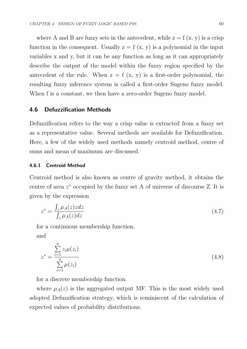
CHAPTER 4. DESIGN OF FUZZY LOGIC BASED PSS 60
where A and B are fuzzy sets in the antecedent, while z = f (x, y) is a crisp
function in the consequent. Usually z = f (x, y) is a polynomial in the input
variables x and y, but it can be any function as long as it can appropriately
describe the output of the model within the fuzzy region specified by the
antecedent of the rule. When z = f (x, y) is a first-order polynomial, the
resulting fuzzy inference system is called a first-order Sugeno fuzzy model.
When f is a constant, we then have a zero-order Sugeno fuzzy model.
4.6 Defuzzification Methods
Defuzzification refers to the way a crisp value is extracted from a fuzzy set
as a representative value. Several methods are available for Defuzzification.
Here, a few of the widely used methods namely centroid method, centre of
sums and mean of maximum are discussed.
4.6.1 Centroid Method
Centroid method is also known as centre of gravity method, it obtains the
centre of area z∗ occupied by the fuzzy set A of universe of discourse Z. It is
given by the expression
z∗ =
∫z µA(z)zdz∫z µA(z)dz
(4.7)
for a continuous membership function,
and
z∗ =
n∑i=1
ziµ(zi)
n∑i=1
µ(zi)(4.8)
for a discrete membership function.
where µA(z) is the aggregated output MF. This is the most widely used
adopted Defuzzification strategy, which is reminiscent of the calculation of
expected values of probability distributions.

CHAPTER 4. DESIGN OF FUZZY LOGIC BASED PSS 61
4.6.2 Centre of Sums (COS) Method
In the centroid method, the overlapping area is counted once whereas in cen-
tre of sums, the overlapping area is counted twice. COS builds the resultant
membership function by taking the algebraic sum of outputs from each of the
contributing fuzzy sets A1, A2, A3,etc. The defuzzified value z∗ is given by
z∗ =
N∑i=1
zi
n∑k=1
µAk(zi)
N∑i=1
n∑k=1
µAk(zi)
(4.9)
where n is the number of fuzzy sets and N is the number of fuzzy variables.
4.6.3 Mean of Maxima (MOM) Method
MOM is the average of the maximizing z∗ at which the MF reach maximum
µ∗. In symbols,
z∗ =
∑ziεM
zi
|M | (4.10)
where M = { zi | µ(zi)the height of the fuzzy set } and |M | is the cardinality
of the set M.
4.7 Design of Fuzzy Logic Based PSS
The basic structure of the fuzzy logic controller is shown in Figure 4.7. Here
the inputs to the fuzzy logic controller are the normalized values of error
’e’ and change of error ’ce’. Normalization is done to limit the universe
of discourse of the inputs between -1 to 1 such that the controller can be
successfully operated within a wide range of input variation. Here ′Ke′ and
′Kce′ are the normalization factors for error input and change of error input
respectively. For this fuzzy logic controller design, the normalization factors
are taken as constants. The output of the fuzzy logic controller is then
multiplied with a gain ′K0′ to give the appropriate control signal ′U ′. The
output gain is also taken as a constant for this fuzzy logic controller.

CHAPTER 4. DESIGN OF FUZZY LOGIC BASED PSS 62
e
ce
1Z
1
eK
1
ceK
eK
ceK
0K
U
Figure 4.7: Basic Structure of Fuzzy Logic Controller
The fuzzy controller used in power system stabilizer is normally a two-
input and a single-output component. It is usually a MISO system. The
two inputs are change in angular speed and rate of change of angular speed
whereas output of fuzzy logic controller is a voltage signal.
4.7.1 Input/output Variables
The design starts with assigning the mapped variables inputs/output of the
fuzzy logic controller (FLC). The first input variable to the FLC is the gen-
erator speed deviation and the second is acceleration. The output variable
to the FLC is the voltage.
After choosing proper variables as input and output of fuzzy controller, it
is required to decide on the linguistic variables. These variables transform
the numerical values of the input of the fuzzy controller to fuzzy quantities.
The number of linguistic variables describing the fuzzy subsets of a variable
varies according to the application. Here seven linguistic variables for each
of the input and output variables are used to describe them. Table 4.1 shows
the Membership functions for fuzzy variables.
The membership function maps the crisp values into fuzzy variables. The

CHAPTER 4. DESIGN OF FUZZY LOGIC BASED PSS 63
NB NEGATIVE BIGNM NEGATIVE MEDIUMNS NEGATIVE SMALLZE ZEROPS POSITIVE SMALLPM POSITIVE MEDIUMPB POSITIVE BIG
Table 4.1: Membership functions for fuzzy variables
triangular membership functions are used to define the degree of membership.
Here for each input variable, seven labels are defined namely, NB, NM, NS,
ZE, PS, PM and PB. Each subset is associated with a triangular membership
function to form a set of seven membership functions for each fuzzy variable.
Figure 4.8: Membership function for speed deviation
Figure 4.9: Membership function for acceleration

CHAPTER 4. DESIGN OF FUZZY LOGIC BASED PSS 64
Figure 4.10: Membership function for voltage
Table 4.2 Decision Table
acceleration
Speed
deviation
NB NM NS ZE PS PM PB
NB NB NB NB NS ZE ZE PS
NM NB NB NM NS ZE PS PM
NS NB NB NM ZE PS PM PB
ZE NB NM NS ZE PS PM PB
PS NB NM NS ZE PM PB PB
PM NM NS ZE PS PM PB PB
PB NS ZE ZE PS PB PB PB
The variables are normalized by multiplying with respective gains Ke,Kce,K0
so that their values lie between -1 and +1. The membership function for speed
deviation, acceleration and voltage are shown in Figure 4.8, Figure 4.9 and
Figure 4.10 respectively.
Knowledge base involves defining the rules represented as IF - THEN rules
statements governing the relationship between input and output variables
in terms of membership functions. In this stage the input variables speed
deviation and acceleration are processed by the inference engine that executes

CHAPTER 4. DESIGN OF FUZZY LOGIC BASED PSS 65
7× 7 rules represented in rule Table 4.2.
Each entity shown in Table 4.2 represent a rule. The antecedent of each
rule conjuncts speed deviation (∆ω) and acceleration (∆a) fuzzy set values.
The knowledge required to generate the fuzzy rules can be derived from
an offline simulation. Some knowledge can be based on the understanding of
the behavior of the dynamic system under control. For monotonic systems, a
symmetrical rule table is very appropriate, although sometimes it may need
slight adjustment based on the behavior of the specific system. If the system
dynamics are not known or are highly nonlinear, trial and error procedures
and experience play an important role in defining the rules.
An example of the rule is: If ∆ω is NS and ∆a is NM then U is NB
which means that if the speed deviation is negative small and acceleration is
negative medium then the output of fuzzy controller should be negative big.
The procedure for calculating the crisp output of the Fuzzy Logic Con-
troller (FLC) for some values of input variables is based on the following
three steps.
Step 1: Determination of degree of firing (DOF) of the rules
The DOF of the rule consequent is a scalar value which equals the mini-
mum of two antecedent membership degrees. For example if ∆ω is PS with
a membership degree of 0.6 and ∆a is PM with a membership degree of 0.4
then the degree of firing of this rule is 0.4.
Step2: Inference Mechanism
The inference mechanism consists of two processes called fuzzy implication
and aggregation. The degree of firing of a rule interacts with its consequent
to provide the output of the rule, which is a fuzzy subset. The formulation
used to determine how the DOF and the consequent fuzzy set interact to form
the rule output is called a fuzzy implication. In fuzzy logic control the most
commonly used method for inferring the rule output is Mamdani method.
Step3: Defuzzification
To obtain a crisp output value from the fuzzy set obtained in the previous
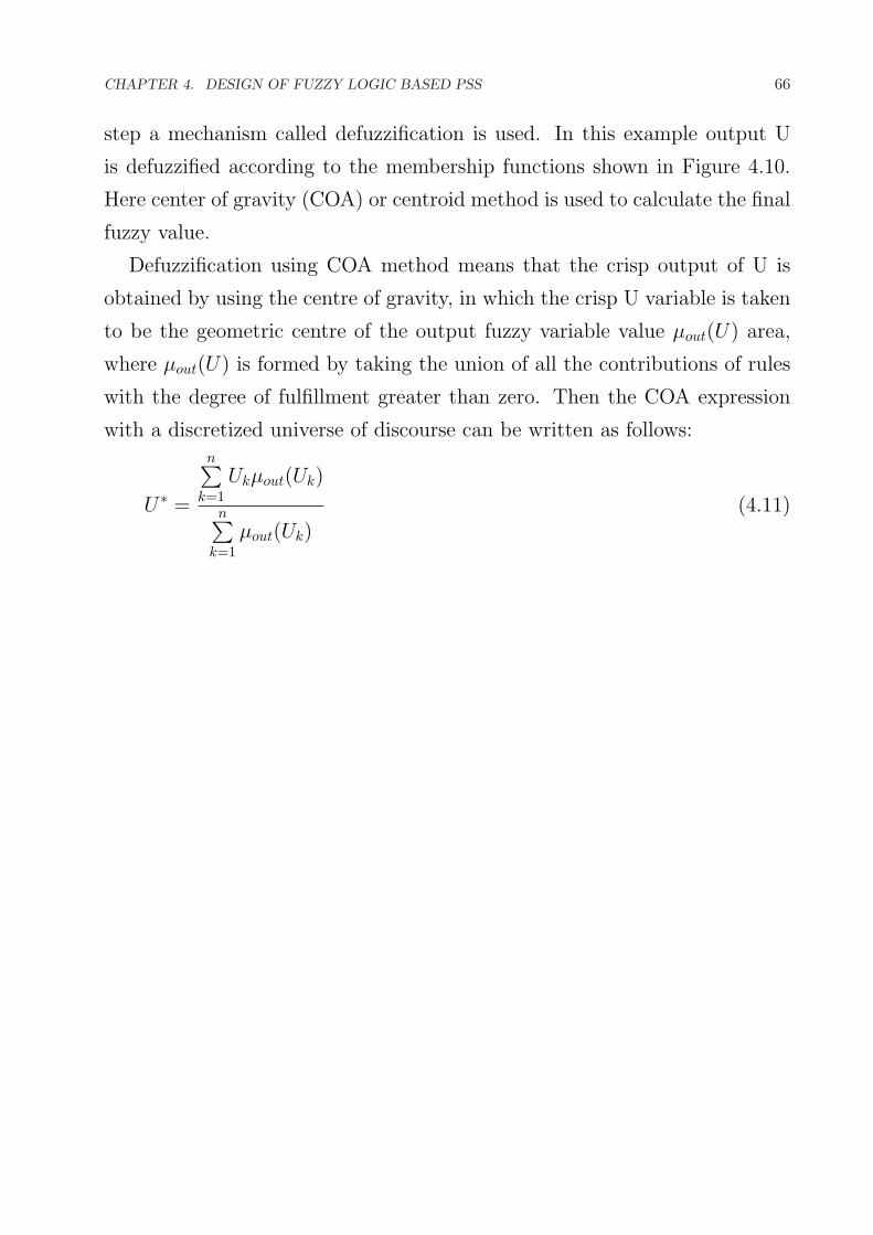
CHAPTER 4. DESIGN OF FUZZY LOGIC BASED PSS 66
step a mechanism called defuzzification is used. In this example output U
is defuzzified according to the membership functions shown in Figure 4.10.
Here center of gravity (COA) or centroid method is used to calculate the final
fuzzy value.
Defuzzification using COA method means that the crisp output of U is
obtained by using the centre of gravity, in which the crisp U variable is taken
to be the geometric centre of the output fuzzy variable value µout(U) area,
where µout(U) is formed by taking the union of all the contributions of rules
with the degree of fulfillment greater than zero. Then the COA expression
with a discretized universe of discourse can be written as follows:
U ∗ =
n∑k=1
Ukµout(Uk)
n∑k=1
µout(Uk)(4.11)
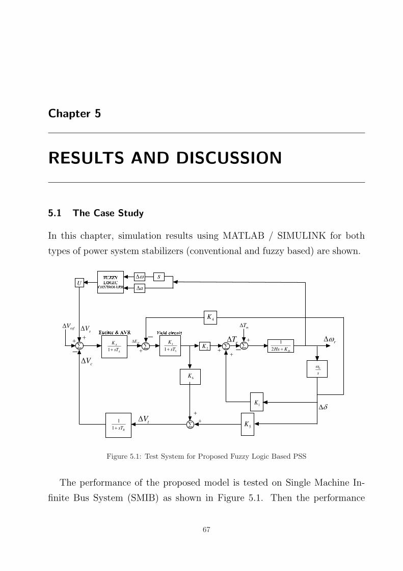
Chapter 5
RESULTS AND DISCUSSION
5.1 The Case Study
In this chapter, simulation results using MATLAB / SIMULINK for both
types of power system stabilizers (conventional and fuzzy based) are shown.
refV
1
1R
sT
1
A
A
K
sT
sV
cV
fdE3
31
K
sT 2K
eT
mT
1
2 DHs K
r
0
s
1K
5Kt
V
6K
4K
Ua
s
Figure 5.1: Test System for Proposed Fuzzy Logic Based PSS
The performance of the proposed model is tested on Single Machine In-
finite Bus System (SMIB) as shown in Figure 5.1. Then the performance
67

CHAPTER 5. RESULTS AND DISCUSSION 68
of SMIB system has been studied without excitation system, with excitation
system only, with conventional PSS (lead-lag) and with fuzzy logic based PSS
by using the K constants. The dynamic models of synchronous machine, ex-
citation system, prime mover, governing system and conventional PSS are
described in chapter 2.
5.2 Performance without Excitation System
In chapter 2, Figure 2.12 shows the block diagram representation with AVR
and PSS. In this presentation, the dynamic characteristics of the system are
expressed in terms of the so-called K - constants. The values of K - constants
calculated using above parameters are
K1 = 1.7299, K2 = 1.7325, K3 = 0.1692, K4 = 2.8543, K5 = −0.0613,
K6 = 0.3954
0 5 10 15 20 25−0.5
0
0.5
1
1.5
2
2.5
3
Time (sec)
Spe
ed D
evia
tion
(p.u
.)
angular speed
angular position
Figure 5.2: response without excitation system
Figure 5.2 shows the variation in angular speed and angular position. From
the above response shown in Figure 5.2 it shows that it is taking very large
time i.e. more than 25 seconds to settle to steady state. Therefore, the
performance of the system with excitation system is analyzed to find the
suitability of the excitation system in removing these oscillations.

CHAPTER 5. RESULTS AND DISCUSSION 69
5.3 Performance with Excitation System
The time response of the angular speed and angular position with excitation
system has shown in Figure 5.3 and Figure 5.4 for positive and negative value
of K5 constant.
From Figure 5.3 the response characteristic shows that under damped
oscillations are resulted. The figure shows that it has negative damping due
to the fact that K5 constant calculated above is negative, which is true for
high values for external system reactance and high generator outputs.
0 1 2 3 4 5 6 7 8 9 10−40
−30
−20
−10
0
10
20
30
40
Time (sec)
Spe
ed D
evia
tion
(p.u
.)
angular speed
angular position
Figure 5.3: Response with excitation system for -ve K5
0 1 2 3 4 5 6 7 8 9 10−0.5
0
0.5
1
1.5
2
2.5
3
3.5
Time (sec)
Spe
ed D
evia
tion
(p.u
.)
angular speed
angular position
Figure 5.4: Response with excitation system for +ve K5
The performance when analyzed with positive value of K5, the system is

CHAPTER 5. RESULTS AND DISCUSSION 70
stable. Positive K5 is possible for low values of external system reactance
and low generator outputs. So for positive the damping is positive and thus
the system is stable.
5.4 Performance with Conventional PSS
Figure 5.5 shows the variation of angular speed and angular position when
PSS (lead-lag) is applied for negative value of K5.
0 1 2 3 4 5 6 7 8 9 10−0.5
0
0.5
1
1.5
2
Time (sec)
Spe
ed D
evia
tion
(p.u
.)
angular speed
angular position
Figure 5.5: Response with CPSS for -ve K5
0 1 2 3 4 5 6 7 8 9 10−0.5
0
0.5
1
1.5
2
2.5
3
Time (sec)
Spe
ed D
evia
tion
(p.u
.)
angular speed
angular position
Figure 5.6: Response with CPSS for +ve K5
From the Figure 5.5 and Figure 5.6 it shows that the system is stable for
both positive and negative value of K5 constant. The transients are more for
negative K5 whereas higher angular position is attained with positive K5.

CHAPTER 5. RESULTS AND DISCUSSION 71
5.5 Performance with Fuzzy Logic Based PSS
The model used in Simulink/Matlab to analyze the effect of fuzzy logic con-
troller in damping small signal oscillations when implemented on single ma-
chine infinite bus system is shown in Figure 5.1.
0 1 2 3 4 5 6 7 8 9 10−0.2
0
0.2
0.4
0.6
0.8
1
1.2
Time (sec)
Spe
ed D
evia
tion
(p.u
.)
angular position
Figure 5.7: Variation of angular position with FLPSS for -ve K5
0 1 2 3 4 5 6 7 8 9 10−0.5
0
0.5
1
1.5
2
2.5
Time (sec)
Spe
ed D
evia
tion
(p.u
.)
angular position
Figure 5.8: Variation of angular position with FLPSS for +ve K5
The variation of angular position with fuzzy logic based PSS for negative
and positive value of K5 constant is shown in Figure 5.7 and Figure 5.8
respectively.
The variation of angular speed with fuzzy logic based PSS for negative
and positive value of K5 constant is shown in Figure 5.9 and Figure 5.10

CHAPTER 5. RESULTS AND DISCUSSION 72
0 1 2 3 4 5 6 7 8 9 10−4
−2
0
2
4
6
8
10
12
14x 10
−3
Time (sec)
Spe
ed D
evia
tion
(p.u
.)
angular speed
Figure 5.9: Variation of angular speed with FLPSS for -ve K5
0 1 2 3 4 5 6 7 8 9 10−2
0
2
4
6
8
10
12
14
16x 10
−3
Time (sec)
Spe
ed D
evia
tion
(p.u
.)
angular speed
Figure 5.10: Variation of angular speed with FLPSS for +ve K5
respectively. Figure 5.7 and Figure 5.9 show that the angular position and
angular speed stabilizes to a particular value with very few oscillations for
negative value of K5constant. For positive value of K5 constant angular
position attains higher value than conventional PSS.
5.6 Performance with different membership functions
Figure 5.11 and Figure 5.12 show the angular position and angular speed
of different membership function (Gaussian, Trapezoidal and Triangular) for
positive value of K5 constant respectively. As shown in Figure 5.11 and Figure
5.12, the oscillations are more pronounced in case of inputs and outputs

CHAPTER 5. RESULTS AND DISCUSSION 73
0 1 2 3 4 5 6 7 8 9 10−0.02
0
0.02
0.04
0.06
0.08
0.1
0.12
0.14
0.16
Time (sec)
Spe
ed D
evia
tion
(p.u
.)
Gaussian
Trapezoidal
Triangular
Figure 5.11: Angular position of different membership function for +ve K5
0 1 2 3 4 5 6 7 8 9 10−1
−0.5
0
0.5
1
1.5x 10
−3
Time (sec)
Spe
ed D
evia
tion
(p.u
.)
Gaussian
Trapezoidal
Triangular
Figure 5.12: Angular speed of different membership function for +ve K5
having trapezoidal membership functions for positive value of K5 and the
system becomes stable after a long time of 8.2 second approximately.
Figure 5.13 and Figure 5.14 show the angular position and angular speed
of different membership function (Gaussian, Trapezoidal and Triangular) for
negative value of K5 constant respectively. As shown in Figure 5.13 and
Figure 5.14, the unstable behavior is resulted if the trapezoidal membership
function is used with negative value of K5 constant. The performance using
gaussian and triangular membership functions is comparable and the system
becomes stable after in nearly 3 second.

CHAPTER 5. RESULTS AND DISCUSSION 74
0 1 2 3 4 5 6 7 8 9 10−0.04
−0.02
0
0.02
0.04
0.06
0.08
0.1
0.12
0.14
Time (sec)
Spe
ed D
evia
tion
(p.u
.)
Gaussian
Trapezoidal
Triangular
Figure 5.13: Angular position of different membership function for -ve K5
0 1 2 3 4 5 6 7 8 9 10−1
−0.5
0
0.5
1
1.5x 10
−3
Time (sec)
Spe
ed D
evia
tion
(p.u
.)
Gaussian
Trapezoidal
Triangular
Figure 5.14: Angular speed of different membership function for -ve K5
5.7 Response for different operating conditions using Triangular MF
Figure 5.15 and Figure 5.16 show the angular position at different operating
conditions for negative and positive value of K5 constant respectively.
Figure 5.17 and Figure 5.18 show the angular speed at different operating
conditions for negative and positive value of K5 constant respectively.
Figure 5.15, Figure 5.16, Figure 5.17 and Figure 5.18 shows the response
for different operating conditions using triangular membership functions and
the result shows that the response is coming out to the stable state with very
few oscillations thus enhancing the stability of a system.
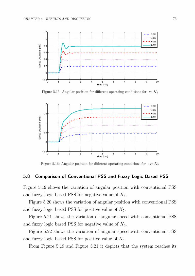
CHAPTER 5. RESULTS AND DISCUSSION 75
0 1 2 3 4 5 6 7 8 9 10−0.2
0
0.2
0.4
0.6
0.8
1
1.2
Time (sec)
Spe
ed D
evia
tion
(p.u
.)
20%
40%
60%
80%
Figure 5.15: Angular position for different operating conditions for -ve K5
0 1 2 3 4 5 6 7 8 9 10−0.5
0
0.5
1
1.5
2
Time (sec)
Spe
ed D
evia
tion
(p.u
.)
20%
40%
60%
80%
Figure 5.16: Angular position for different operating conditions for +ve K5
5.8 Comparison of Conventional PSS and Fuzzy Logic Based PSS
Figure 5.19 shows the variation of angular position with conventional PSS
and fuzzy logic based PSS for negative value of K5.
Figure 5.20 shows the variation of angular position with conventional PSS
and fuzzy logic based PSS for positive value of K5.
Figure 5.21 shows the variation of angular speed with conventional PSS
and fuzzy logic based PSS for negative value of K5.
Figure 5.22 shows the variation of angular speed with conventional PSS
and fuzzy logic based PSS for positive value of K5.
From Figure 5.19 and Figure 5.21 it depicts that the system reaches its
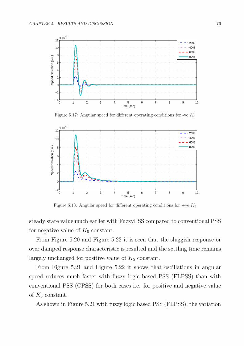
CHAPTER 5. RESULTS AND DISCUSSION 76
0 1 2 3 4 5 6 7 8 9 10−4
−2
0
2
4
6
8
10
12x 10
−3
Time (sec)
Spe
ed D
evia
tion
(p.u
.)
20%
40%
60%
80%
Figure 5.17: Angular speed for different operating conditions for -ve K5
0 1 2 3 4 5 6 7 8 9 10−2
0
2
4
6
8
10
12x 10
−3
Time (sec)
Spe
ed D
evia
tion
(p.u
.)
20%
40%
60%
80%
Figure 5.18: Angular speed for different operating conditions for +ve K5
steady state value much earlier with FuzzyPSS compared to conventional PSS
for negative value of K5 constant.
From Figure 5.20 and Figure 5.22 it is seen that the sluggish response or
over damped response characteristic is resulted and the settling time remains
largely unchanged for positive value of K5 constant.
From Figure 5.21 and Figure 5.22 it shows that oscillations in angular
speed reduces much faster with fuzzy logic based PSS (FLPSS) than with
conventional PSS (CPSS) for both cases i.e. for positive and negative value
of K5 constant.
As shown in Figure 5.21 with fuzzy logic based PSS (FLPSS), the variation

CHAPTER 5. RESULTS AND DISCUSSION 77
0 1 2 3 4 5 6 7 8 9 10−0.015
−0.01
−0.005
0
0.005
0.01
0.015
0.02
Time (sec)
Spe
ed D
evia
tion
(p.u
.)
FLPSS
CPSS
Figure 5.19: Comparison of angular position between CPSS and FLPSS for -ve K5
0 1 2 3 4 5 6 7 8 9 10−0.5
0
0.5
1
1.5
2
2.5
3
Time (sec)
Spe
ed D
evia
tion
(p.u
.)
FLPSS
CPSS
Figure 5.20: Comparison of angular position between CPSS and FLPSS for +ve K5
in angular speed reduces to zero in about 2 to 3 seconds but with conventional
PSS (CPSS), it takes about 6 seconds to reach to the final steady state value
and also the oscillations are less pronounced in FLPSS.
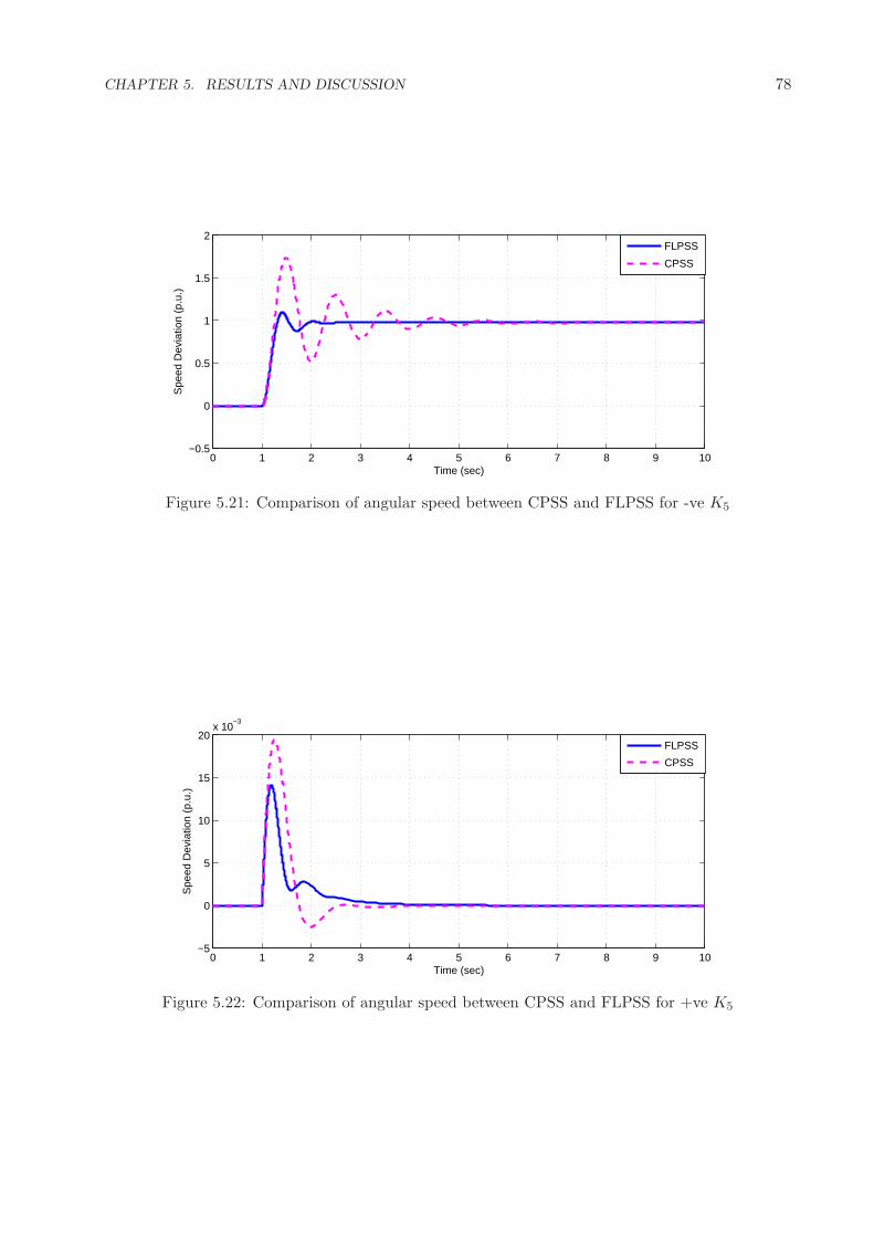
CHAPTER 5. RESULTS AND DISCUSSION 78
0 1 2 3 4 5 6 7 8 9 10−0.5
0
0.5
1
1.5
2
Time (sec)
Spe
ed D
evia
tion
(p.u
.)
FLPSS
CPSS
Figure 5.21: Comparison of angular speed between CPSS and FLPSS for -ve K5
0 1 2 3 4 5 6 7 8 9 10−5
0
5
10
15
20x 10
−3
Time (sec)
Spe
ed D
evia
tion
(p.u
.)
FLPSS
CPSS
Figure 5.22: Comparison of angular speed between CPSS and FLPSS for +ve K5

Chapter 6
CONCLUSION AND SUGGESTIONS
FOR FUTURE WORK
6.1 Conclusion
In this thesis work initially the effectiveness of power system stabilizer in
damping power system stabilizer is reviewed. Then the fuzzy logic based
power system stabilizer is introduced by taking speed deviation and accel-
eration of synchronous generator as the input signals to the fuzzy controller
and voltage as the output signal. FLPSS shows the better control perfor-
mance than power system stabilizer in terms of settling time and damping
effect. Therefore, it can be concluded that the performance of FLPSS is
better than conventional PSS. However, the choice of membership functions
has an important bearing on the damping of oscillations. From the sim-
ulation studies it shows that the oscillations are more pronounced in case
of trapezoidal membership functions. The response with gaussian member-
ship functions is comparable to triangular membership functions. However,
the performance of FLPSS with triangular membership functions is superior
compared to other membership functions.
79

CHAPTER 6. CONCLUSION AND SUGGESTIONS FOR FUTURE WORK 80
6.2 Suggestions for future work
Having gone through the study of fuzzy logic based PSS (FLPSS) for single
machine infinite bus system, the scope of the work is
1. The fuzzy logic based PSS (FLPSS) can be extended to multi machine
interconnected system having non-linear industrial loads which may in-
troduce phase shift.
2. The fuzzy logic based PSS with frequency as input parameter can be
investigated because the frequency is highly sensitive in weak system,
which may offset the controller action on the electrical torque of the
machine.
3. Testing using more complex network models can be carried out.
Bibliography
[1] T. Abdelazim and O. Malik, “An adaptive power system stabilizer using on-line self-learning fuzzysystems,” in Power Engineering Society General Meeting, 2003, IEEE, vol. 3, july 2003, pp. 1715 –1720 Vol. 3.
[2] A. Al-Hinai, “Dynamic stability enhancement using genetic algorithm power system stabilizer,” inPower System Technology (POWERCON), 2010 International Conference on, oct. 2010, pp. 1 –7.
[3] K. Al-Olimat, A. Farhoud, and J. Hurtig, “Power system stabilizers with fuzzy logic switching,” inPower Systems Conference and Exposition, 2006. PSCE ’06. 2006 IEEE PES, 29 2006-nov. 1 2006, pp.2152 –2157.
[4] P. M. Anderson, A. A. Fouad, and H. H. Happ, “Power system control and stability,” Systems, Manand Cybernetics, IEEE Transactions on, vol. 9, no. 2, p. 103, feb. 1979.
[5] A. Babaei, S. Razavi, S. Kamali, and A. Gholami, “Performance improvement of power system sta-bilizer by genetic algorithm for one machine infinite bus system,” in Universities Power EngineeringConference, 2007. UPEC 2007. 42nd International, sept. 2007, pp. 344 –348.
[6] M. Basler and R. Schaefer, “Understanding power system stability,” in Protective Relay Engineers, 200558th Annual Conference for, april 2005, pp. 46 – 67.
[7] H. Behbehani, J. Bialek, and Z. Lubosny, “Enhancement of power system stability using fuzzy logicbased supervisory power system stabilizer,” in Power and Energy Conference, 2008. PECon 2008. IEEE2nd International, dec. 2008, pp. 479 –484.
[8] W.-C. Chan and Y.-Y. Hsu, “An optimal variable structure stabilizer for power system stabilization,”Power Apparatus and Systems, IEEE Transactions on, vol. PAS-102, no. 6, pp. 1738 –1746, june 1983.
[9] A. Chatterjee, S. Ghoshal, and V. Mukherjee, “A comparative study of single input and dual input powersystem stabilizer by hybrid evolutionary programming,” in Nature Biologically Inspired Computing,2009. NaBIC 2009. World Congress on, dec. 2009, pp. 1047 –1052.
[10] D. Chaturvedi, O. Malik, and P. Kalra, “Experimental studies with a generalized neuron-based powersystem stabilizer,” Power Systems, IEEE Transactions on, vol. 19, no. 3, pp. 1445 – 1453, aug. 2004.
[11] C.-J. Chen, T.-C. Chen, H.-J. Ho, and C.-C. Ou, “Pss design using adaptive recurrent neural networkcontroller,” in Natural Computation, 2009. ICNC ’09. Fifth International Conference on, vol. 2, aug.2009, pp. 277 –281.
81
BIBLIOGRAPHY 82
[12] W. Chi-Jui and H. Yuan-Yih, “Design of self-tuning pid power system stabilizer for multimachine powersystems,” Power Systems, IEEE Transactions on, vol. 3, no. 3, pp. 1059 –1064, aug 1988.
[13] J. H. Chow and J. J. Sanchez-Gasca, “Pole-placement designs of power system stabilizers,” PowerEngineering Review, IEEE, vol. 9, no. 2, pp. 60 –61, feb. 1989.
[14] J. Chow, G. Boukarim, and A. Murdoch, “Power system stabilizers as undergraduate control designprojects,” Power Systems, IEEE Transactions on, vol. 19, no. 1, pp. 144 – 151, feb. 2004.
[15] F. Demello and C. Concordia, “Concepts of synchronous machine stability as affected by excitationcontrol,” Power Apparatus and Systems, IEEE Transactions on, vol. PAS-88, no. 4, pp. 316 –329, april1969.
[16] T. L. DeMello F.P., P.J. Nolan and J. Undrill, “coordinated application of stabilizers in multi machinepower system,” Proceedings of the Twenty-First Annual North-American Power Symposium, vol. Issue,9-10, pp. 175 – 184., july 1989.
[17] M. Dobrescu and I. Kamwa, “A new fuzzy logic power system stabilizer performances,” in PowerSystems Conference and Exposition, 2004. IEEE PES, oct. 2004, pp. 1056 – 1061 vol.2.
[18] A. Dysko, W. Leithead, and J. O’Reilly, “Enhanced power system stability by coordinated pss design,”Power Systems, IEEE Transactions on, vol. 25, no. 1, pp. 413 –422, feb. 2010.
[19] R. Gupta, B. Bandyopadhyay, and A. Kulkarni, “Design of power system stabiliser for single-machinesystem using robust periodic output feedback controller,” Generation, Transmission and Distribution,IEE Proceedings-, vol. 150, no. 2, pp. 211 – 216, march 2003.
[20] R. Gupta, D. Sambariya, and R. Gunjan, “Fuzzy logic based robust power system stabilizer for multi-machine power system,” in Industrial Technology, 2006. ICIT 2006. IEEE International Conference on,dec. 2006, pp. 1037 –1042.
[21] S. Gupta, N; Jain, “Comparative analysis of fuzzy power system stabilizer using different membershipfunctions,,” International Journal of Computer and Electrical Engineering, vol. 2, no. 2, april. 2010.
[22] G. Gurrala and I. Sen, “A modified heffron-phillip’s model for the design of power system stabiliz-ers,” in Power System Technology and IEEE Power India Conference, 2008. POWERCON 2008. JointInternational Conference on, oct. 2008, pp. 1 –6.
[23] ——, “Power system stabilizers design for interconnected power systems,” Power Systems, IEEE Trans-actions on, vol. 25, no. 2, pp. 1042 –1051, may 2010.
[24] T. Hussein, A. Elshafei, and A. Bahgat, “Design of a hierarchical fuzzy logic pss for a multi-machinepower system,” in Control Automation, 2007. MED ’07. Mediterranean Conference on, june 2007, pp.1 –6.
[25] T. Hussein, M. Saad, A. Elshafei, and A. Bahgat, “Damping inter-area modes of oscillation using anadaptive fuzzy power system stabilizer,” in Control and Automation, 2008 16th Mediterranean Confer-ence on, june 2008, pp. 368 –373.
[26] G.-H. Hwang, J.-H. Park, H. T. Kang, and S. Kim, “Design of fuzzy power system stabilizer usingadaptive evolutionary algorithm,” in Industrial Electronics, 2000. ISIE 2000. Proceedings of the 2000IEEE International Symposium on, vol. 1, 2000, pp. 42 –47 vol.1.

BIBLIOGRAPHY 83
[27] A. Jalilvand, R. Aghmasheh, and E. Khalkhali, “Robust design of pid power system stabilizer in multi-machine power system using artificial intelligence techniques,” in Power Engineering and OptimizationConference (PEOCO), 2010 4th International, june 2010, pp. 38 –42.
[28] S. Kamalasadan and G. Swann, “A novel power system stabilizer based on fuzzy model referenceadaptive controller,” in Power Energy Society General Meeting, 2009. PES ’09. IEEE, july 2009, pp. 1–8.
[29] M. Kothari and T. Kumar, “A new approach for designing fuzzy logic power system stabilizer,” inPower Engineering Conference, 2007. IPEC 2007. International, dec. 2007, pp. 419 –424.
[30] P. Kundur., “Power system control and stability,” New York: McGraw-Hill, vol. PAS-88, pp. 1103–1166,1994.
[31] E. Larsen and D. Swann, “Applying power system stabilizers part i, ii, iii: Practical considerations,”Power Apparatus and Systems, IEEE Transactions on, vol. PAS-100, no. 6, pp. 3034 –3046, june 1981.
[32] Y. Lin, “Systematic approach for the design of a fuzzy power system stabiliser,” in Power SystemTechnology, 2004. PowerCon 2004. 2004 International Conference on, vol. 1, nov. 2004, pp. 747 – 752Vol.1.
[33] J. Lu, M. Nehrir, and D. Pierre, “A fuzzy logic-based adaptive power system stabilizer for multi-machinesystems,” in Power Engineering Society Summer Meeting, 2000. IEEE, vol. 1, 2000, pp. 111 –115 vol.1.
[34] M. M. M. F. Othman and D. Linkens, “Designing power system stabilizer for multi machine powersystem using neuro-fuzzy algorithm,” jurnal Teknologi, pp. 55–64, 2001.
[35] F. M. H. M. Saidy, “Performance improvement of a conventional power system stabilizer,” InternationalJournal of Electrical Power and Energy Systems, vol. 150, no. 5, pp. 313–323, oct. 2005.
[36] J. Matsuki, T. Okada, and K. Sakurai, “Experimental approach to optimal setting of parameters infuzzy control algorithm for power system stabilization,” in Industrial Electronics, Control, and Instru-mentation, 1993. Proceedings of the IECON ’93., International Conference on, nov 1993, pp. 273 –278vol.1.
[37] N. Nallathambi and P. Neelakantan, “Fuzzy logic based power system stabilizer,” in E-Tech 2004, july2004, pp. 68 – 73.
[38] K. R. Padiyar, “Power system dynamics: Stability and control,” in printed in the Republic of Singapore,ISBN: 0-471-19002-0, 1996.
[39] Y.-M. Park, U.-C. Moon, and K. Lee, “A self-organizing power system stabilizer using fuzzy auto-regressive moving average (farma) model,” Energy Conversion, IEEE Transactions on, vol. 11, no. 2,pp. 442 –448, jun 1996.
[40] G. Radman and Y. Smaili, “Performance evaluation of pid power system stabilizer for synchronousgenerator,” in Southeastcon ’88., IEEE Conference Proceedings, apr 1988, pp. 597 –601.
[41] M. Ramirez-Gonzalez and O. Malik, “Simplified fuzzy logic controller and its application as a powersystem stabilizer,” in Intelligent System Applications to Power Systems, 2009. ISAP ’09. 15th Interna-tional Conference on, nov. 2009, pp. 1 –6.
BIBLIOGRAPHY 84
[42] F. Rashidi, M. Rashidi, and H. Amiri, “An adaptive fuzzy sliding mode control for power systemstabilizer,” in Industrial Electronics Society, 2003. IECON ’03. The 29th Annual Conference of theIEEE, vol. 1, nov. 2003, pp. 626 – 630 vol.1.
[43] G. Rogers, “Demystifying power system oscillations,” Computer Applications in Power, IEEE, vol. 9,no. 3, pp. 30 –35, jul 1996.
[44] A. Roosta, H. Khorsand, and M. Nayeripour, “Design and analysis of fuzzy power system stabilizer,”in Innovative Smart Grid Technologies Conference Europe (ISGT Europe), 2010 IEEE PES, oct. 2010,pp. 1 –7.
[45] A. Singh and I. Sen, “A novel fuzzy logic based power system stabilizer for a multimachine system,” inTENCON 2003. Conference on Convergent Technologies for Asia-Pacific Region, vol. 3, oct. 2003, pp.1002 – 1006 Vol.3.
[46] D. Sumina, N. Bulic, and G. Erceg, “Simulation model of neural network based synchronous generatorexcitation control,” in Power Electronics and Motion Control Conference, 2008. EPE-PEMC 2008.13th, sept. 2008, pp. 556 –560.
[47] A. E. T. Hussein, M.S. Saad and A. Bahgat, “Robust adaptive fuzzy logic power system stabilizer,” AnInternational Journal, vol. 36, no. 10, dec. 2009.
[48] A. Taher, S.A.; Shemshadi, “Design of robust fuzzy logic power system stabilizer,” World Academy ofScience, Engineering and Technology, no. 27, 2007.
[49] H. Toliyat, J. Sadeh, and R. Ghazi, “Design of augmented fuzzy logic power system stabilizers toenhance power systems stability,” Energy Conversion, IEEE Transactions on, vol. 11, no. 1, pp. 97–103, mar 1996.
[50] J. Van Ness, F. Brasch, G. Landgren, and S. Naumann, “Analytical investigation of dynamic instabilityoccuring at powerton station,” Power Apparatus and Systems, IEEE Transactions on, vol. PAS-99,no. 4, pp. 1386 –1395, july 1980.
[51] M. Vani, G. Raju, and K. Prasad, “Robust supplementary controllers for avr and pss,” in India Con-ference (INDICON), 2009 Annual IEEE, dec. 2009, pp. 1 –4.
[52] C. Vournas and J. Mantzaris, “Application of qss modeling to stabilizer design for interarea oscillations,”Power Systems, IEEE Transactions on, vol. 25, no. 4, pp. 1910 –1917, nov. 2010.
[53] W. Watson and G. Manchur, “Experience with supplementary damping signals for generator staticexcitation systems,” Power Apparatus and Systems, IEEE Transactions on, vol. PAS-92, no. 1, pp. 199–203, jan. 1973.
[54] S. K. Yee and J. Milanovic, “Fuzzy logic controller for decentralized stabilization of multimachine powersystems,” Fuzzy Systems, IEEE Transactions on, vol. 16, no. 4, pp. 971 –981, aug. 2008.
[55] Y.-N. Yu and Q.-H. Li, “Pole-placement power system stabilizers design of an unstable nine-machinesystem,” Power Systems, IEEE Transactions on, vol. 5, no. 2, pp. 353 –358, may 1990.

Appendices
85

Appendix A
System Data
The Parameters of the synchronous machine, excitation system and conven-
tional PSS are as follows.
[a] Synchronous machine constants: xd= 2.64 pu, x′d= 0.28 pu
xq= 1.32 pu, x′q= 0.29 pu
RE= 0.004 pu, XE= 0.73 pu
f= 60 Hz, H= 4.5 sec
[b] Excitation system constants: KA= 100, TA= 0.05, TR= 0.015
EFMAX= 5.0, EFMIN= -5.0
[c] PSS constants: KSTAB= 20, Tw= 1.4 sec
T1= 0.154 sec, T2= 0.033 sec
VSMAX= 0.2, VSMIN= -0.2
86
LIST OF PUBLICATIONS
[1] Kamalesh Chandra Rout, P.C. Panda, ”Improvement of dynamic stability
of a single machine infinite bus power system using fuzzy logic based power
system stabilizer”, International Conference on Electrical Power and Energy
Systems (ICEPES - 2010), Aug 26 - 28, 2010, NIT Bhopal.
[2] Kamalesh Chandra Rout, P.C. Panda, ”Power system dynamic stability
enhancement of SMIB using fuzzy logic based power system stabilizer”, Inter-
national Conference on Advances in Power Electronics and Instrumentation
Engineering (PEIE - 2010) Sep 07 - 08, 2010, Kochi, Kerala.
[3] Kamalesh Chandra Rout, P.C. Panda, ”An adaptive fuzzy logic based
power system stabilizer for enhancement of power system stability”, IEEE
International Conference on Industrial Electronics, Control and Robotics
(IECR - 2010), Dec 27 - 30, 2010 NIT Rourkela.
[4] Kamalesh Chandra Rout, P.C. Panda, ”Performance analysis of power
system dynamic stability using fuzzy logic based PSS for positive and neg-
ative value of K5 constant”, IEEE International Conference on Computer,
Communication and Electrical Technology (ICCCET - 2011), March 18 - 19,
2011, NCE, Tirunelvelli.
87

AUTHOR’S BIOGRAPHY
Kamalesh Chandra Rout was born to Sri Kailash Chandra Rout and Smt.
Promodini Rout on 26th June, 1981 at Dhenkanal, Odisha, India. He ob-
tained a Bachelors degree in Electrical Engineering from University College
of Engineering (U.C.E), Burla, Odisha in 2004. He joined the Department of
Electrical Engineering, National Institute of Technology, Rourkela in January
2009 as an Institute Research Scholar to pursue M.Tech by Research.
88