Dynamic Supply Chain Structuring for

Electronic Commerce Among Agents�

Daniel Dajun Zeng

Katia Sycara

Graduate School of Industrial Administration

The Robotics Institute

Carnegie Mellon University

Pittsburgh, PA 15213, USA

Abstract

Electronic commerce and the vast amounts of real-time informa-tion available through means of EDI and the Internet are reshaping theway enterprises conduct business. A new computational infrastruc-ture and models are needed for a business to gain a competitive edgethrough e�ective use of this information base. One of the key issuesin competing in the electronic marketplace is product/service di�eren-tiation. Currently there are no computational models for multi-issuedecision making in electronic commerce.

We develop a model of inter-organizational electronic commercethat explores various new choices and opportunities that the electronicmarketplace o�ers. The particular motivating applications of our workare supply chain management. Two major performance measures ofsupply chain activities are cost and leadtime. In our model, we explic-itly address these two issues in a uni�ed fashion for a variety of supplychain activities, such as outsourcing, supplier selection, production ca-pacity, transportation mode selection, and inventory positioning. We

� This research has been sponsored in part by ONR Grant No. N00014-96-1-1222, and

by NSF grant #IRI-9612131.

1

model di�erent business entities as autonomous software agents inter-connected via the Internet. The main research focus of our e�orts ishow to coordinate software agents in supply chains dynamically and exibly such that goods and services can be delivered at the right timein a cost-e�ective manner.

The supply chain structure is modeled by an AND/OR network.We develop an eÆcient algorithm for software agents in supply chainsto evaluate the alternatives that o�er di�erent leadtime and cost pa-rameters. We have coupled this model with operational level decisionmaking such as stochastic inventory management. Experimental re-sults show that our model results in signi�cant improvement in solu-tion quality as compared to traditional models.

1 Introduction

Current networking technology and the ready availability of vast amountsof real-time data and information on the Internet-based Infosphere bring tobusiness decision makers more abundant and accurate information. Manyonline businesses specialize in delivering electronic catalog services and per-forming other intermediary functions such as business/product yellowpageand matchmaking. Emerging computing paradigms such as Internet-basedsoftware agents are also making locating and accessing information increas-ingly easier.

Electronic commerce is reshaping both consumer market and inter-organizationalbusiness. How to compete in the electronic marketplace e�ectively poses sig-ni�cant challenges to practitioners and researchers. In this paper, we focuson inter-organizational electronic commerce in the context of supply chainmanagement. Researchers and practitioners have observed that the natureof competition in electronic commerce does not resemble undi�erentiatedBertrand competition. This suggests that price alone is not the only decisioncriterion. Other decision criteria related with product/service di�erentiationneed to be considered. Two of the prominent performance measures of a sup-ply chain are cost and leadtime. By leadtime, we mean the amount of timethat elapses from the instant that an order (or service request) is placed untilit arrives. By cost, we mean the sum of the costs of all activities requiredto satisfy the order (or deliver the service). Some examples of these supplychain activities and decisions are:

2

� Supplier selection. Procurement management is playing an increas-ingly important role nowadays with the globalization of manufacturingand advances in network information infrastructure. There usually ex-ists a rich set of suppliers o�ering raw materials of varying quality, cost,and delivery leadtime. Decisions regarding supplier selection have tobe made after a careful evaluation of the impact of raw material costand delivery time responsiveness on the supply chain as a whole.

� bf Subcontracting. In manufacturing, managers face \make or buy"decisions|the choice between making components/products in houseor subcontracting them to outside sources. When making in houseis not an option or is clearly suboptimal, management has to selectthe appropriate subcontractors from a pool of potential subcontractorsthat o�er di�erent levels of service under di�erent prices. These deci-sions are critical in today's highly competitive and dynamic businessenvironment.

� Transportation mode selection. Typically, multiple transportationmodes are available to supply chain managers, o�ering a wide range ofcost/time options. Decisions regarding which mode is best suited forthe current order are dependent on how urgently the order needs to be�lled, how expensive these modes are, and where this transportationactivity is located in the supply chain network.

� Assembly/subassembly. Assembly/subassembly operations cannotstart until all the components/subcomponents/raw materials requiredbecome available. Production managers need to make sure that allthese materials are accessible for use at the right place and the righttime.

� Production rate decision. Production rate decisions correspondwith the choice between using faster, more expensive, high-capacityproduction facilities versus slower but cheaper facilities. To evaluatethe tradeo�s between these options is not trivial considering all theupstream and downstream activities in the supply chain.

In this paper, we present a model of inter-organizational electronic com-merce that explicitly addresses the time and cost issues in a uni�ed fash-ion. We model di�erent business entities as autonomous software agents

3

interconnected via the Internet. These agents act on behalf of their hu-man users/organizations in order to perform laborious information gatheringtasks, such as locating and accessing information from various on-line infor-mation sources, �lter away irrelevant or unwanted information, and providedecision support. Section 1.1 discusses some of the related literature. Sec-tion 2 presents a brief description of our supply chain model, called LCT(Leadtime-Cost-Tradeo�). The LCT model needs to be integrated with otheroperational level decision making models such as inventory management toenable intelligent agents to make the full range of supply chain decisions.Section 3 presents how to integrate LCT into the EOQ model where the de-mand rate is assumed to be constant. We present in Section 4 our model andanalysis of stochastic inventory management given the leadtime/cost choices.Experimental results show that our model results in signi�cant improvementin solution quality as compared to traditional models. Computing optimalpolicies for the resulting model proves to be computationally diÆcult. Sec-tion 5 presents a computational study of making inventory decisions that takeadvantage of leadtime/cost options. We conclude the paper in Section 6 bysummarizing the results and pointing out other extensions to our agent-basedmulti-issue supply chain model.

1.1 Related Literature

E�ective use of the Internet by individual users, organizations, or decisionsupport machine systems has been hampered by some dominant character-istics of the Infosphere. Information available from the net is unorganized,multi-modal, and distributed on server sites all over the world. The avail-ability, type and reliability of information services are constantly changing.In addition, information is ambiguous and possibly erroneous due to the dy-namic nature of the information sources and potential information updatingand maintenance problems. The notion of Intelligent Software Agents (e.g.,[WJ95, SZ96]) has been proposed to address this challenge. In this paper,we model a supply chain as a multi-agent system where di�erent businessentities interact with one another through intelligent software agents thatact on their behalf. In general, multi-agent systems can compartmentalizespecialized task knowledge, organize themselves to avoid processing bottle-necks, and can be built expressly to deal with dynamic changes in the agentand information-source landscape. In addition, Multiple Intelligent Agents

4

are ideally suited to the predominant characteristics of the Infosphere (and inparticular supply chain management), such as the heterogeneity of the infor-mation sources, the diversity of information gathering and decision supporttasks that the gathered information supports, and the presence of multipleusers/organizations with related information and decision aiding needs.

In order for autonomous software agents to make sensible decisions inany nontrivial domain such as supply chain management, they need to haveaccess to domain-speci�c decision making models and related computationalmechanisms[LS97]. We brie y survey some of these models in literature thatare most relevant to multi-issue (time and cost) supply chain management.

The �rst models that consider the possibility of purchasing shorter lead-times at a premium cost appeared in [Bul64] and [Fuk64], among others.The main objective of these papers is to �nd the optimal ordering policythat minimizes ordering, holding and penalty costs when subject to randomdemand. Structural results regarding the optimal replenishment policy wereestablished when there are only two options and the leadtimes of the twooptions di�er by one time unit (in periodic review situations).

Kaplan in [Kap70] analyzed optimal policies for a dynamic inventoryproblem when the leadtime is a discrete random variable with known dis-tribution. Assuming that outstanding orders do not cross in time, Kaplanderived the structure of optimal policies which is shown to be similar to thoseobtained with deterministic leadtimes. Although [Kap70] is not concernedwith di�erent leadtime options, it gives a good survey for the technical diÆ-culties that we also encountered.

Song and others in [Son94] studied the impact of stochastic leadtimes onthe optimal inventory decisions and the optimal cost in a base-stock inven-tory model. The focus there is to evaluate the impact of the variability ofleadtimes but not to derive an inventory policy which makes use of the avail-ability of multiple leadtime/cost options. In [LZ93] Lau and Zhao consideredthe order splitting between two suppliers that o�er di�erent leadtime withuncertainty. The authors assumed a constant splitting ratio among two sup-pliers and developed computational methods to compute the optimal ratio,ordering quantities and reordering point in a continuous review inventorysetting. Several papers (e.g., [BDR94]) deal with situations where leadtimesis one of the decision variables. Their assumption is that by paying \leadtimecrashing cost" leadtime reduction can be achieved. The goal of these papersis to �nd the single best leadtime option under single sourcing.

5

2 The LCT Supply Chain Model

We have developed a supply chain model, called LCT, based on an AND/ORnetwork representation[HZ97]. This model is capable of capturing a varietyof supply chain activities and decisions.

In LCT, a supply chain is modeled as a directed acyclic graph with paral-lel arcs. The model follows an activity-on-arc representation where each arccorresponds to a particular supply chain activity (production, transporta-tion, subcontracting, etc.). Note that each activity/arc has two performancemeasures: leadtime and cost. In this supply chain network, nodes representcompletion of activities and may be used to establish precedent constraintsamong activities. The graph is directed towards one particular \root node".The root node corresponds to the retailer of the product that the supply chainproduces. End customers interact with the root node only. We de�ne twotypes of nodes that each speci�es conditions for satisfying prior activities:conjunction and disjunction nodes. Conjunction nodes or AND nodes arenodes for which all the activities that correspond to the incoming arcs mustbe accomplished before the outgoing activities can begin; whereas disjunc-tion nodes or OR nodes requires that at least one of the incoming activitiesmust be �nished before the outgoing activities can begin.

Based on LCT we have developed eÆcient computation methods to iden-tify the entire eÆcient frontier between leadtime and cost in supply chains.This eÆcient frontier at the \root node", i.e., the retailer point, compactlyrepresents all the undominated, feasible combinations of supply chain activ-ities. By a feasible combination of supply chain activities, we mean the setof activities that guarantee the availability of goods or services at the rootnode. We say a combination dominates the other when the former o�erscheaper cost and shorter leadtime than the latter. Given the eÆcient fron-tier coupled with the market demand pro�le and pricing strategy at the rootnode, management can converge on the optimal tradeo� point specifying aparticular supply chain con�guration.

One of the limitations of LCT is that the model doesn't explicitly considerinventory. Without inventory, the solution concept based on the leadtimecost eÆcient frontier applies to \one-shot" scenarios in which single perioddemand is considered at the root node (e.g., make-to-order). If demand forthe end product is repetitive, holding inventory at one or more places inthe supply chain clearly has the potential of improving the performance of

6

the whole system. The rest of the paper focuses on integrating LCT withinventory management|out �rst step to extend LCT to address multi-perioddemand.

In this paper, we assume that inventory can be held only at the rootnode1. In other words, we are concerned with integrating one stage inven-tory management within the context of LCT. Since we only add the inventorycapacity at the root node, the entire eÆcient frontier between leadtime andcost in the supply chain network remains the same. We are interested in waysthrough which the end product retailer can take advantage of the availabil-ity of multiple options with varying leadtime and cost parameters. Despitethe restrictive assumption made in this model as to the inventory location,this model captures the fundamental characteristics of a variety of supplychain management situations. For instance, the model is readily applicablefor retailers who may get goods/services from various manufacturers thatquote di�erent unit price and delivery leadtime. In another example, a man-ufacturing �rm is structuring its international sourcing base. Suppose thatthis �rm adopts a make-to-stock policy. Our model can be applied to makesourcing decisions based on the current inventory stock level.

3 LCT in Inventory Models with Constant

Demand Rates

In this section, we demonstrate how the LCT model can be integrated intoinventory models that assume constant demand rates.

Let l denote the leadtime, UP (l) the cheapest unit ordering cost for goodsfor which the order ful�llment takes at most l. The leadtime cost eÆcientfrontier computed in LCT takes the form of the function UP (l). When theleadtime measure can be properly discretized (e.g., in units of days), UP (l)is a step function:

UP (l) = ci if i � l < i+ 1 for i = 0; 1; : : : ;M

whereM is the maximum leadtime from all possible alternatives and ci is theminimum unit ordering cost if the target leadtime is expected to be strictly

1The extension of LCT which allows inventory at arbitrary nodes in the supply chain

network is beyond the scope of this paper.

7

less than i+1. Without loss of generality, we assume that ci is nonincreasingwith respect to i.

Let SK(l) denote the setup cost associated with selecting the cheapestsupply chain con�guration that achieves leadtime l.

SK(l) = Ki if i � l < i + 1 for i = 0; 1; : : : ;M

The total ordering cost TC(x; l) for x units of product with the leadtimerequirement l is given by

TC(x; l) = Ki + cix if i � l < i+ 1 for i = 0; 1; : : : ;M

We follow the standard assumptions of the EOQ inventory model: Thedemand rate � is constant; no stockout or backlogging is allowed. Considerthe following situation which is a special case of our model. There is only onealternative available that o�ers leadtime k, setup cost K, and unit orderingprice c. The optimal ordering policy in this case is well known. It followsthe (Q;R) policy, where Q is the standard EOQ quantity, R is the reorderpoint which is equal to k�. (We assume k � Q=� for simplicity.)

Let's consider the general case where more than one alternatives are avail-able. We only consider the cycle inventory which is the amount of inventoryphysically on hand at any point in time. The optimal ordering policy involvesusing the alternative with leadtime i� which is de�ned as follows:

�ci� +q2Ki��h � min

i(�ci +

q2Ki�h)

This implies a single sourcing policy will be optimal. Search for i� canbe easily done by enumerating all available modes. It is clear that whenKi is nonincreasing with respect to i, the least expensive alternative thatalso o�ers the longest leadtime is always the mode of choice. After thealternative i� has been chosen, the classical (Q;R) policy can be used todetermine the order amount and reorder point. Obviously, other extensionssuch as �nite production capacity can be done in the same fashion withoutcausing additional technical problems.

8

4 LCT in Periodic Review Stochastic Inven-

tory Model

In the previous section, we show that integrating LCT with inventory modelswith constant demand rates can be easily done. When we consider inven-tory management with uncertain demand, however, the situation changesdramatically. In this section, we �rst present a formal formulation of theproblem and then proves some formal properties. We demonstrate the tech-nical diÆculties of �nding optimal policies and motivate our computationalwork (presented in Section 5) in �nding e�ective suboptimal policies.

We study an N -period stochastic inventory problem in which there arem di�erent ordering options. These options represent di�erent leadtime andcost tradeo�s which can be computed using the LCT model given the networktopology of a supply chain and time/cost information for the supply chainactivities. We ignore the setup cost in this study2.

We use the following notation in our study. Most of the notation followsthe standard one used inN -period single-stage stochastic inventory modeling:

N = the number of periods in the planning horizon

m = the number of delivery/production options. We assume that m < N .

�i = the leadtime associated with option i, i = 1; 2; : : : ; m. We assumethat these leadtimes are deterministic. Without loss of generality, weassume that �i < �j when i < j.

� = the maximum leadtime from all possible options. � = �m

ci = the unit ordering cost with option i, i = 1; 2; : : : ; m. We assume thatci > cj when i < j3.

t = the demand for the item during each period. We assume that the demandis stationary.

e(x+) = the salvage value of having x+ = max(x; 0) units of inventory onhand at the end of the period N . We assume e(x+) is convex.

2It is not entirely arbitrary since electronic commerce contributes to the setup cost

reduction.3This is not a restriction. See the discussion in Section 4.3

9

� = the one-period discount factor

x1 = the current stock level

x2; x3; : : : ; x� = the outstanding orders such that x2 is due at the start ofthe next period, x3 is to be delivered two periods hence, etc.

zi = the amount of goods to be ordered at the start of the present periodusing option i, i = 1; 2; : : : ; m. These are the inventory decision vari-ables.

L(x) = the expected operational costs during the period, exclusive of order-ing costs, w.r.t. the stock on hand at the beginning of the period:

L(x) =

( R x0 h(x� t)f(t)dt+

R1x p(t� x)f(t)dt x > 0;R1

0 p(t� x)f(t)dt x � 0(1)

We assume that the holding cost h(�) and penalty cost p(�) are non-decreasing and convex. The unful�lled ordered are backlogged. Sinceintegration preserves the convexity, the convexity of L(x) is easily seen.

Cn(x1; x2; � � � ; x� ) = the minimum expected cost following an optimal policy,given that only n future periods are to be taken into account, where(x1; x2; : : : ; x� ) represents all the information about the current stocklevel as well as the amounts of goods whose orders have been submittedand are to be delivered during the following � � 1 periods.

To simplify the notation, we also use the following vector-based represen-tations:

x : the row vector of (x1; x2; : : : ; x� )

z : the row vector of (z1; z2; : : : ; zm)

The functional equation for Cn(�) is easily seen to be

Cn(x1; x2; : : : ; x� ) = minzi�0;for 1�i�m

� mXi=1

cizi + L(x1 + y0) + (2)

+�Z 10

Cn�1(x1 + y0 � t + x2; x2 + y1; � � � ; x� + y��1; y�)f(t)dt�

(3)

10

where, yi is de�ned as follows:

yi =

(z�j

if i = �j;0 otherwise

(4)

Under these assumptions, we can prove the convexity of the value func-tion.

Theorem 1 Cn(x) is convex.

Proof. We prove Theorem 1 by induction. Given the cost structure of thesalvage value,

C0(x) = p(x�1 ) + e(x+1 ) (5)

C0(x) is convex.By induction on Cn�1, we will prove that Cn is also convex. We �rst

introduce some auxiliary vectors to simplify the notation. De�ne

g(x; z; t) � Cn�1(A

264xzt

375) (6)

where A is a � � (� +m+ 1) matrix. Each element of A, Aij, is given asfollows:

Aij =

8>>>>>><>>>>>>:

1 if i = 1 and j = 1;�1 if i = 1 and j = � +m + 1;1 if j = i + 1 for all i 2 [1; � � 1];1 if �j = i for all j 2 [� + 1; � +m];0 otherwise

(7)

It can be easily veri�ed that the functional equation (2) can be rewrittenas:

Cn(x) = minz

� mXi=1

cizi + L(x + y0) + �Z 10

g(x; z; t)f(t)dt�

(8)

Given that Cn�1 is convex and that A is a full-rank linear transformation,g(x; z; t) is convex due to [Roc70] Theorem 5.7 Part A.

11

De�neq(x; z) =

Z 10

f(t)g(x; z; t)dt (9)

We know that q(x; z) is convex since f(t) � 0 due to [Ash72].Since the operating cost L is convex, and q is convex, we conclude that

the summationPm

i=1 cizi + L(x + y0) + q(x; z) is convex. Due to [Roc70]Theorem 5.7 Part B, we know that Cn is convex.

4.1 Optimal Inventory Control Policy

Karlin and Scarf in [AKS58] studied inventory models in the presence ofa time lag. Their models can be viewed as a special case of ours sincethey assumed that there is only one leadtime option available. Based onthe convexity of the objective function, they proved that the optimal policyfollows an order-up-to policy. Simply put in our notation, if m = 1, z�1 =(S � (x1 + x2 + :::+ x�1))

+, S being the order-up-to level to be determined.Fukuda in [Fuk64] extended this result to deal with 2-mode cases. Again,based on the convexity of the objective function, he proved that the optimalcontrol policy is very similar to an order-up-to policy except for an additionalstock level up to which it is desired to order using the quicker and moreexpensive option. The intuition is that to use quicker option to handle large,unexpected demand while the steady portion of the demand ow is handledby the slower and less expensive option. In both cases, the optimal inventorypolicies are not diÆcult to compute.

One might think that the similar intuition may be extended to the gen-eral m option case by having m order-up-to levels for each leadtime op-tion. Unfortunately, this is not the case. By solving a very simple 2-mode(�1 = 0; �2 = 2) problem, we found that no simple order-up-to or order-up-to like structures exists. The complexity of the problem is coming from thefact that although the convexity of the objective function holds, the optimalcontrols are functions of all the xi for i = 1; 2; : : : ; � rather than functions ofP�

i=1 xi.Using the value iteration approaches in dynamic programming, we can

compute the optimal control policies regardless of whether they follow theorder-up-to structure or not. However, these value iterations approaches arealmost impossible to scale up since the size of state space itself is exponential

12

with respect to the maximum leadtime. For practical purposes, we need to�nd other more eÆcient algorithms.

The same technical diÆculties have been identi�ed in di�erent inventorymanagement and dynamic programming settings. (e.g.,[Kap70]). In orderto get analytically appealing results, the standard way of avoiding thesediÆculties in inventory management is to assume that at any certain moment,there is only one outstanding order. This is clearly not our option, since whatwe are interested is precisely using multiple options at the same time.

To address these computational issues, we have developed several sub-optimal polices that are easy to compute. In Section 5, we reported thesepolicies and an experimental evaluation of their performances. To illustratethe signi�cance of making use of multiple leadtime options, in Section 4.2 weuse a numerical example to demonstrate that using multiple leadtime optionscan result in signi�cant improvement in solution quality. As a side result,we establish in Section 4.3 a simple dominance relationship among leadtimeoptions that can be used to eliminate certain options from considerationwithout compromising the solution quality. Admittedly, this dominance re-lationship does not help in worse case scenarios where no leadtime options aredominated by others. It could, however, save some computation by throwingout the dominated options.

4.2 An Numerical Example: The Value of Having Mul-

tiple Leadtime Options

In this section, we use a numerical example to demonstrate that havingmultiple leadtime options can result in signi�cant improvement as comparedto having one (Karlin and Scarf's model) or two leadtime options where theleadtime di�erence is 1 time unit (Fukuda's model).

Consider the following scenario. We assume that one period demand isdiscretely distributed according to the following probability mass function:

d 0 1 2 3 4p(d) 0.2 0.2 0.2 0.2 0.2

To construct a comparison baseline, we �rst start o� with using one lead-time option only. We are interested in minimizing the in�nite horizon average

13

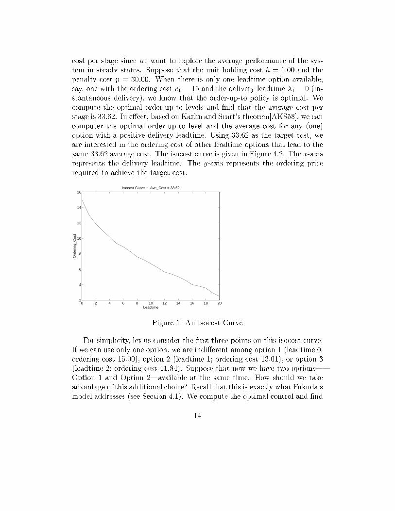
cost per stage since we want to explore the average performance of the sys-tem in steady states. Suppose that the unit holding cost h = 1:00 and thepenalty cost p = 30:00. When there is only one leadtime option available,say, one with the ordering cost c1 = 15 and the delivery leadtime �1 = 0 (in-stantaneous delivery), we know that the order-up-to policy is optimal. Wecompute the optimal order-up-to levels and �nd that the average cost perstage is 33.62. In e�ect, based on Karlin and Scarf's theorem[AKS58], we cancomputer the optimal order-up-to level and the average cost for any (one)option with a positive delivery leadtime. Using 33.62 as the target cost, weare interested in the ordering cost of other leadtime options that lead to thesame 33:62 average cost. The isocost curve is given in Figure 4.2. The x-axisrepresents the delivery leadtime. The y-axis represents the ordering pricerequired to achieve the target cost.

0 2 4 6 8 10 12 14 16 18 202

4

6

8

10

12

14

16Isocost Curve − Ave_Cost = 33.62

Leadtime

Ord

erin

g_C

ost

Figure 1: An Isocost Curve

For simplicity, let us consider the �rst three points on this isocost curve.If we can use only one option, we are indi�erent among option 1 (leadtime 0;ordering cost 15.00), option 2 (leadtime 1; ordering cost 13.01), or option 3(leadtime 2; ordering cost 11.84). Suppose that now we have two options|Option 1 and Option 2|available at the same time. How should we takeadvantage of this additional choice? Recall that this is exactly what Fukuda'smodel addresses (see Section 4.1). We compute the optimal control and �nd

14

the average cost decreases from 33.62 to 30.46. Using option 2 and option 3results in a average cost of 30.55, computed similarly.

How about using these three options together? Since the size of the prob-lem is very small, we can a�ord to enumerate all the states in the state spaceand compute the optimal control for each state. We use a linear programcoded in AMPL to compute the minimal steady state average cost. The re-sult is 27.18. Percentage wise, it represents a 19.16% decrease in operatingcost from 33.62 (using one option only), which is quite signi�cant.

This example reinforces our intuitive notion that by dynamically com-bining these multiple leadtime options contingent on the current inventoryposition and outstanding orders, the system can achieve lower cost. Due tothe complex interactions between these leadtime options, we could not �nd ananalytically elegant solution. Nevertheless, this model presents an abstrac-tion of realistic supply chain management scenarios and could potentiallyo�er signi�cant bene�ts. This has motivated our work in developing compu-tational methods to construct suboptimal yet e�ective policies, reported inSection 5.

4.3 A Simple Dominance Relationship

As we discussed in Section 4.1, considering all leadtime options poses seriouscomputational challenges. In this section, we establish a simple dominancerelationship which, when applicable, helps reduce computational e�orts byexcluding certain options|the dominated ones|without compromising thesolution quality.

The intuition behind this dominance relationship is quite obvious: forany option i, if there is another option j that o�ers either quicker deliveryunder same ordering cost, or o�ers lower price while ensuring same delivery,or o�ers both lower price and quicker delivery, option i will never be used inthe optimal controls and therefore can be ignored. In this case, we say i isdominated by j. The following lemma formalizes this notion.

Lemma 1 An option i with leadtime �i and ordering cost ci is dominated

by another option j with leadtime �j and ordering cost cj when ci � cj and�i � �j. There always exist an optimal control policy which does not use

option i.

15

The proof is straightforward. Consider the set of all the control policiesthat use option i, denoted by !i. For each control ui 2 !i, substitute option jfor option i as follows: if �i = �j, simply use option j whenever i is used. If�i > �j, use option j whenever i is used but delay the orderings by �i � �j.It is clear that the resulted control policy after substitution costs equal to orless than the original control policy ui that uses option i. Since this is truefor any arbitrary ui, the lemma immediately follows.

5 Computing Inventory Policies with Multi-

ple Leadtime Options

For computational purposes, we assume that demand is a discrete randomvariable. For problems that have small maximum leadtime from all options(say, the maximum leadtime � < 4) and do not require �ne-granularity de-mand discretization, the optimal policy can be found either by policy iter-ation through linear programming or value iteration through dynamic pro-gramming [Ber95]. Both linear programming and dynamic programming re-quire the explicit storage of the state space. Since the size of the state spacegrows exponentially with the maximum leadtime, neither linear program-ming nor dynamic programming can be used to solve large-sized problems(say, with more than 5 options). To give an example how quickly the sizeof the state space becomes unmanageable, consider the following scenario:Suppose that we have 5 leadtime options whose delivery leadtimes are 1,2, 3, 4, 5, respectively. Furthermore, suppose that one-period demand isa discrete random variable that takes on values from zero up to 20. Theminimum number of the states required by value iteration using dynamicprogramming is in the order of magnitude of 1074. To maintain such a largestate space and compute optimal control for each and every state repeatedlytill the value function converges is not practical. Neither can policy iterationhandle computation of this size.

In this section, we propose three suboptimal control policies that are eas-ier to compute than the optimal policies. The performance of these policies

4We do not consider the complications at the boundaries of the state space when

we compute this minimum number of states required. In practice, larger state space is

necessary to ensure that value iteration returns reliable results.

16

is evaluated via simulation.

5.1 The Dynamic Switching Policy

By the dynamic switching policy, we mean the policy that uses only oneleadtime option at each ordering point but does not require the same optionto be used at di�erent ordering points. This type of policy has a naturemapping in practice: \do not split orders between suppliers at each orderingpoint; but switch among suppliers in di�erent time periods if needed". Usingour notation, this means:

mXi=1

zi = zj for some j: 1 � j � m (10)

In order to search for the optimal policies within the set of dynamicswitching policies, we still need to explicitly represent the state space andtherefore we are limited to solving small-sized problem instances. However,to compute the optimal controls (how much to order using which option) foreach state for the dynamic switching policy is much easier as compared to�nding the true optimal controls for each state in general due to the factthat choices are much limited. In addition to its favorable computationalproperties, we are interested in dynamic switching polices because of itsmanagerial implications.

5.2 The Echelon Order-up-to Policy

It is clear that we cannot a�ord to explicitly carry around the state spacein order to solve large-sized problems. One way of avoiding representingthe state space is to apply the idea of parameterize the control policies. Weconsider a class of controls that can be characterized by a small number of pa-rameters. Based on these parameters, we can easily deduce the correspondingcontrol for any given arbitrary state. For instance, consider an one-optioninventory model (See Section 4.1), an order-up-to policy is characterized byone parameter order-up-to level S. Given any state x (the current inventoryposition), the control (order amount) is (S � x)+. This way, the originalproblem of �nding optimal control policies is transformed into �nding thebest parameters S� that minimizes the overall system cost. Note that in this

17

case, we do not need to explicitly record and visit each state in the statespace.

Note that for our general m-option inventory problems, the order-up-to policy or its variants have been proved nonoptimal. The simplicity ofthe order-up-to policy and its wide acceptance in practice, however, haverendered itself as a good candidate suboptimal policy in which we are in-terested. In our study, we consider the following policy fashioned after theorder-up-to policy.

zi = (Si �

�iXj=1

xj �i�1Xj=1

zj)+ for i = 1; : : : ; m (11)

We call this the \echelon order-up-to policy" due to the similarity betweenthis policy and the policies developed in multi-echelon inventory research[CS60]. Intuitively, we can imagine that for each leadtime option, thereis an \order-up-to" level that guarantees that the sum of future arrivalsand committed orders using quicker options reaches a predetermined level.The rationale behind this is similar to that behind Fukuda's policy for twoadjacent (in terms of leadtimes) options. As long as we have enough inventoryon hand and on order, we use slow options. The costly quick options are usedto handle situations where shortage occurs.

5.3 The Separating Planes Policy

As we will report in Section 5.4, although the echelon order-up-to policy iseasy to compute and can be used to solve large-sized problems, the resultingsolution quality measured by the average per stage cost is not entirely satis-factory. To achieve lower and closer-to-optimal costs, we develop the follow-ing policy which can be viewed as a generalization of the echelon order-up-topolicy.

zi = (�i ��X

j=1

�ijxj)+ for i = 1; : : : ; m (12)

Recall that when we follow an echelon order-up-to policy, we weigh allthe xj and zj equally. We analyzed a number of the optimal policies (forsmall-sized problems) produced by policy iteration or value iteration andobserved that equally weighing xj and zj clearly violates optimality. In

18

the meantime, to a large extent, the points in the high-dimensional spaceof (x1; x2; : : : ; xm; zj) for j = 1; 2; : : : ; m can be separated by hyperplanes.These hyperplanes are not necessarily in parallel. This motivates the devel-opment of the separating plane policy. This policy, like the echelon order-up-to policy, does not require explicit representation of the state space andtherefore can be used in solving large-sized problem instances. The sepa-rating plane policy involves more parameters than the echelon order-up-topolicy and therefore are more computationally intensive. Using the separat-ing plane policy, however, results in lower average per state system cost, asdemonstrated in Section 5.4.

5.4 Experimental Comparisons

To evaluate the e�ectiveness of the proposed control policies, we performedthe following experiments. We generated 396 problem instances by varyingthe number of leadtime options available, demand pro�les and cost parame-ters summarized below:

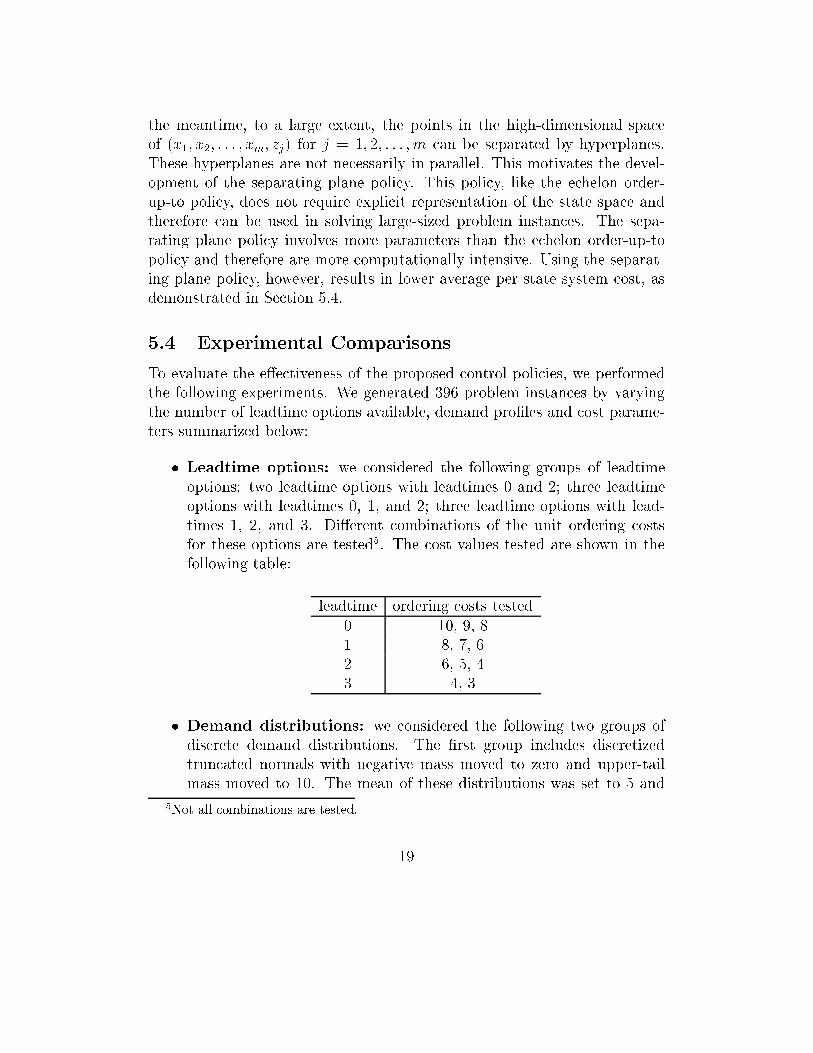
� Leadtime options: we considered the following groups of leadtimeoptions: two leadtime options with leadtimes 0 and 2; three leadtimeoptions with leadtimes 0, 1, and 2; three leadtime options with lead-times 1, 2, and 3. Di�erent combinations of the unit ordering costsfor these options are tested5. The cost values tested are shown in thefollowing table:

leadtime ordering costs tested0 10, 9, 81 8, 7, 62 6, 5, 43 4, 3

� Demand distributions: we considered the following two groups ofdiscrete demand distributions. The �rst group includes discretizedtruncated normals with negative mass moved to zero and upper-tailmass moved to 10. The mean of these distributions was set to 5 and

5Not all combinations are tested.

19

the following standard deviations were tested: .5, 1, 2, 5, 10. The sec-ond group is consisted of 10 distributions with one period demand ttaking on values from 0 to 3. The tested probability mass functions aregiven in the following table.

probability mass functionp(t = 0) p(t = 1) p(t = 2) p(t = 3)

1 0.25 0.25 0.25 0.252 0.8 0.05 0.05 0.13 0.1 0.05 0.05 0.84 0.1 0.8 0.05 0.055 0.05 0.05 0.8 0.16 0.4 0.35 0.05 0.2

� Cost parameters: the holding cost per period is always set to 1. Wetested two values of the penalty cost per period: 15 and 30.

We developed the simulation testbed in the C programming language. Allexperiments were performed on a Sun Ultra-1 machine. Table 1 representsthe summarized results. Results of the policies are stated as percentage excessover the optimal cost which was obtained using value iterations. Table 2records the average amount of time in CPU minutes that it took to computethe policies for one problem instance. Little attempt was made to make thecoding eÆcient, so these time �gures should be viewed with caution.

Leadtime Dynamic Echelon SeparatingOptions Switching Order-up-to Plane2 modes (0, 2) 15.3 11.6 5.43 modes (0, 1, 2) 16.2 12.2 6.23 modes (1, 2, 3) 18.7 12.1 6.3

Table 1: Average Performance of Policies Considered (% Error)

From these experimental �ndings, we make the following observations:the dynamic switching policy is easy to compute (for small-sized problems)

20

Leadtime Optimal Dynamic Echelon SeparatingOptions Policy Switching Order-up-to Plane2 modes (0, 2) 12.2 0.3 0.9 1.93 modes (0, 1, 2) 12.4 0.3 4.8 11.43 modes (1, 2, 3) 200.0 3.2 4.9 12.8

Table 2: Average CPU time of Computing Policies Considered (in minutes)

but the solution quality measured by the average per stage cost is not sat-isfactory (16.2% above the optimal cost on grand average). The echelonorder-up-to policy takes a moderate computational e�ort to compute andyields reasonable results (11.9% above the optimal). The separating planepolicy takes relatively intensive computational e�orts to compute but yieldsvery good results (5.8% above the optimal cost).

We have also conducted experiments for problem instances of larger size(maximum leadtimes ranging from 4 to 6) using the echelon order-up-to andthe separating plane policies. For these problems, optimal policies are notknown since neither value iteration nor policy iteration can be applied be-cause of the size of the problem. In addition, the dynamic switching policycannot be used due to the size of the state space. Initial experimental re-sults suggest that the echelon order-up-to and the separating plane policiesare capable of handling large-sized problems and the separating place policyoutperforms the echelon order-up-to policy by roughly the same percentagewhich we observed for the small-sized problems. Further investigation isneeded to determine how e�ective these policies are, possibly through estab-lishing lower bounds on the average cost.

6 Concluding Remarks

Inter-organizational electronic commerce is reshaping the way enterprisesconduct business. In this paper, we present a model of supply chain thatexplicitly addresses time and cost issues. We have coupled this model withinventory management and performed a computational study to �nd e�ectivecontrol policies. These models and computational mechanisms are essential

21

for software agents to take advantage of abundant choices that come withthe increasingly accessible worldwide information infrastructure, and to gaincompetitive edge in highly dynamic business environments.

We conclude this paper by presenting some of the extensions to our agent-based supply chain model.

� Other performance measures of supply chains such as product quality,service levels, etc., are not addressed in our current model. We plan toenrich our model to address these additional measures.

� Our current model assumes that cost/leadtime information associatedwith each supply chain activity is known and deterministic. In prac-tice, more often than not uncertainty will arise, especially in leadtime.Models that deal with the stochastic leadtime is highly desirable. Wehave proved that �nding stochastic leadtime/cost eÆcient frontier isintractable if using the �rst order stochastic dominance alone. We arecurrently working on identifying other stochastic dominance relation-ships (possibly of the heuristic nature) that cut down computation.

� In this paper, we discussed how to integrate inventory decisions intothe LCT model. We assumed that inventory is held at the root of thesupply chain. We are currently working on integrating LCT with multi-echelon production/inventory models. Current multi-echelon inventoryliterature typically is not concerned with leadtime issues. To evaluatethe impact of leadtime options in a multi-echelon setting is signi�cant.The main research issues are: how to measure and evaluate the overallperformance of such a complex supply chain, how to make inventorypositioning decisions, how to compute eÆciently multi-echelon inven-tory policies with leadtime options, etc.

22

References

[AKS58] Kenneth J. Arrow, Samuel Karlin, and Herbert Scarf. Studies in

the Mathematical Theory of Inventory and Production. StanfordUniversity Press, 1958.

[Ash72] Robert B. Ash. Real Analysis and Probability. Probability andMathematical Statistics. Academic press, 1972.

[BDR94] M. Ben-Daya and Abdul Raouf. Inventory models involving leadtimes as a decision variable. Journal of Operational Research So-

ciety, 45(5):579{582, 1994.

[Ber95] Dimitri P. Bertsekas. Dynamic Programming and Optimal Control.Athena Scienti�c, 1995.

[Bul64] E. Bulinskaya. Some results concerning optimum inventory policies.Theory of Probability and its Applications, 9(3):389{403, 1964.

[CS60] A. Clark and H. Scarf. Optimal policies for a multi-echelon inven-tory problem. Management Science, 6(4):475{490, 1960.

[Fuk64] Y. Fukuda. Optimal policies for the inventory problem with nego-tiable leadtime. Management Science, 10(4):690{708, 1964.

[HZ97] Arthur Hsu and Dajun Zeng. Finding ordering policies given mul-tiple leadtime options. Graduate School of Industrial Administra-tion, working paper, Carnegie Mellon University, 1997.

[Kap70] Robert S. Kaplan. A dynamic inventory model with stochastic leadtimes. Management Science, 16(7):491{507, 1970.

[LS97] J.S. Liu and K. Sycara. Coordination of multiple agents for pro-duction management. Annals of Operations Research, 75:235{289,1997.

[LZ93] Hon-Shiang Lau and Long-Geng Zhao. Optimal ordering policieswith two suppliers when lead times and demands are all stochastic.European Journal of Operational Research, 68:120{133, 1993.

23

[Roc70] R. Tyrrell Rockafellar. Convex Analysis. Princeton UniversityPress, 1970.

[Son94] Jing-Sheng Song. The e�ect of leadtime uncertainty in a simplestochastic inventory model. Management Science, 40(5):603{613,May 1994.

[SZ96] Katia Sycara and Dajun Zeng. Coordination of multiple intelligentsoftware agents. International Journal of Cooperative Information

Systems, 5(2 & 3):181{211, 1996.

[WJ95] M. Wooldridge and N. R. Jennings. Intelligent agents: Theory andpractice. The Knowledge Engineering Review, 10(2):115{152, 1995.

24