dynamic transmission error measurementshomel.vsb.cz/~tum52/publications/te_measurements.pdf · an...

Engineering Mechanics Jiri Tuma, Page number

1

DYNAMIC TRANSMISSION ERROR MEASUREMENTS

Jiří Tůma

VSB – Technical University of Ostrava, Faculty of Mechanical Engineering Department of Control Systems and Instrumentation

17. listopadu 15 CZ-708 33 Ostrava, Czech Republic

[email protected]

Abstract The paper deals with the dynamic transmission error (TE) measurements of a simple gear set at gearbox operational conditions that means under load and during rotation. The analysis method is focused on the processing of impulse signals generated by incremental rotary encoders attached to both the gears in mesh. The analysis technique benefits from demodulation of a phase-modulated signal. The theory is illustrated by experiments with a car gearbox and measurement errors are discussed.

Key words: gears, transmission error, measurement, Fourier transform, Hilbert transform, Hilbert transformer, analytic signal.

Introduction Mechanical power is transmitted from a driving gear to the driven gear by means of force TF acting along the line of action. This force is balanced by the same and antiparallel force SF acting at the shaft support point. The simultaneous acting of the force couple TF and SF to the driven gear results in torque, see Figure 1. The teeth contact stiffness is not a constant but it is oscillating in synchronism with tooth meshing frequency due to the variation of the number of tooth pairs in contact and moving the teeth contact point along the tooth flank. The variation of the tooth contact stiffness causes the self excited angular vibration of the driven gear, which results in the time varying forces TF and SF . The force acting at the shaft support is dynamic as well and excites the vibration of the gearbox housing and consequently radiating noise.

Therefore, noise and vibration problems in gearing are mainly concerned with the smoothness of the drive. The parameter that is employed to measure smoothness is the Transmission Error (TE) [1]. This parameter can be expressed as a linear displacement at a base circle radius defined by the difference of the output gear’s position from where it would be if the gear teeth were perfect and infinitely stiff. Many references have attested to the fact that a major goal in reducing gear noise is to reduce the transmission error of a gear set. Experiments [2] show that decreasing TE by 10 dB results in decreasing transmission sound level by 7

Fig. 1. Main source of gearbox

vibration and noise

Line of action

Pitch circle

Support point

FT FS


2

dB. This paper is focused at the problem of TE measurement as a part of the experimental

study of the tooth contact dynamics. These measurements can contribute not only to the theoretical modeling, which is well developed, for instance, by [3], but to gear design improvements [4]. Low noise, high load capacity and long time servicing gears are a result of employing the high contact ratio tooth design. The effect of improving design can be experimentally tested by TE measurements. The introductory chapters deal with the measurement principles based on the phase demodulation of the impulse signals. The signal processing methods employs the Hilbert transform [5]. There are two approaches to evaluate this transformation, both of them are discussed. As a part of this paper, the first experimental results are presented here. It can be highlighted that the measurements were done on the true transmission unit and at operational condition.

Angular vibration measurements TE results from angular vibration. There are many possible methods for angular vibration measurement during rotation

• Tangentially mounted accelerometers • Laser torsional vibration meter based on the Doppler effect • Incremental rotary encoders (several hundreds of impulses per revolution)

There are many possible approaches to measuring TE as well, but, as Derek Smith points out in his book [6], in practice, measurements based on the use of incremental rotary encoders dominates. Instantaneous angular velocity is proportional to the reciprocal value of the time interval, which is elapsed between consecutive impulses. The measurement methods for the length of the time interval are as follows

• Sample number & Interpolation • High frequency oscillator (1 or 10 GHz) & Impulse counter • Phase demodulation.

The simplest method for evaluation of the instantaneous rotational speed is the reciprocal value of the time interval between two consecutive impulses. If the impulse signal is sampled then the time interval between the adjacent impulses is determined by interpolation some 50 times more accurately than indicated by the actual sampling interval. The accuracy is satisfying for the RPM measurement based on only one impulse per shaft rotation. This method is not suitable if the large number of impulses per revolution is generated, which results in a few samples between impulses and the time interval length is impossible to estimate at satisfying accuracy. If the string of encoder impulses as an analogue signal controls a gate for the high frequency clock signal (100 MHz or 1 GHz), which is an input of an impulse counter, then this method works properly. This principle is implemented in the signal analyzers produced by Rotec. The instantaneous angular velocity is primary information for TE evaluation and needs integration with respect to time. Henriksson and Pärssinen present an example of this measurement [8]. The methods based on using the Hilbert transformation give as primary information the instantaneous rotation angle.

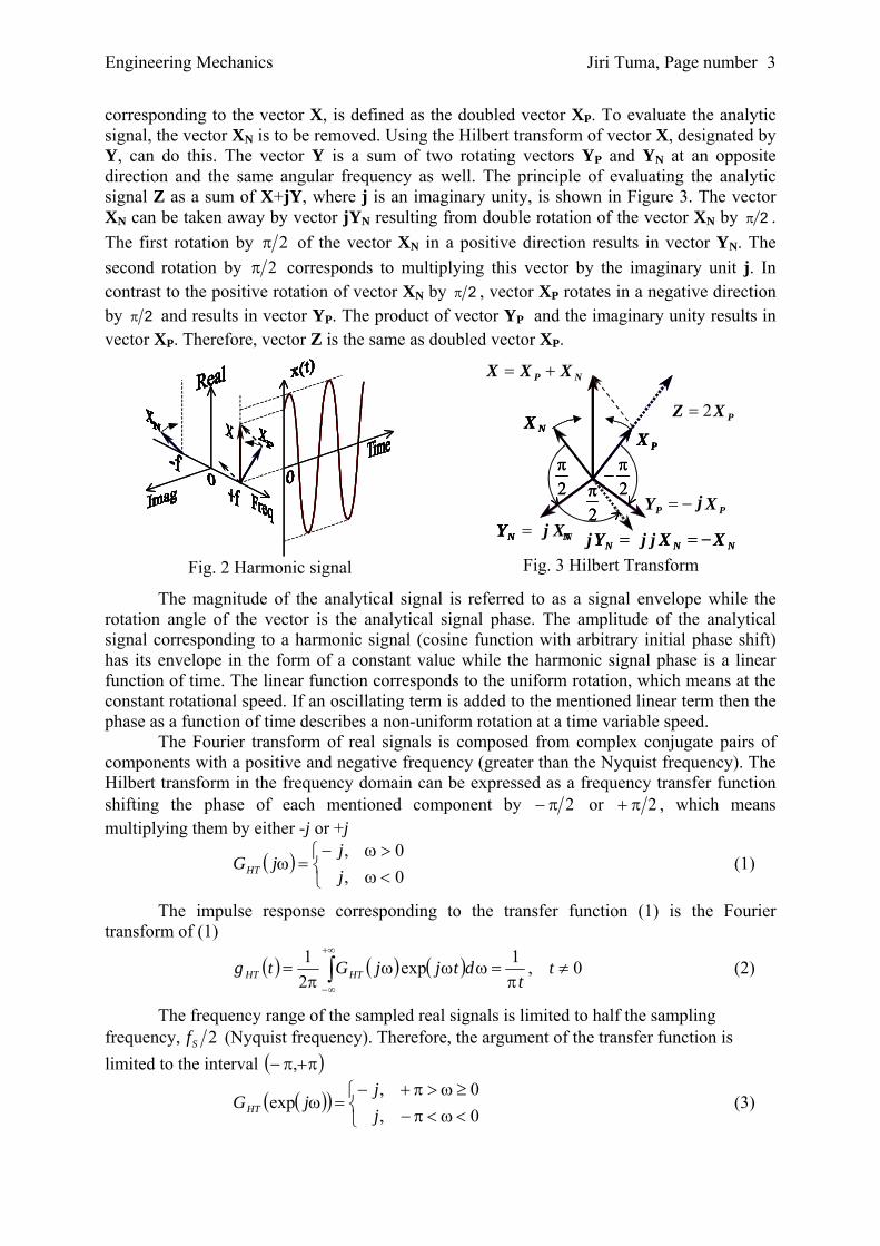
Hilbert transformation The real harmonic signal X can be modeled in the complex plane as a sum of two rotating vectors, XP and XN, at the same angular frequency but the opposite direction. The vector X is parallel to the real axis if both these vectors are complex conjugate; it means that they are of the same magnitude and opposite initial phase, see Figure 2. The analytical signal,


3

corresponding to the vector X, is defined as the doubled vector XP. To evaluate the analytic signal, the vector XN is to be removed. Using the Hilbert transform of vector X, designated by Y, can do this. The vector Y is a sum of two rotating vectors YP and YN at an opposite direction and the same angular frequency as well. The principle of evaluating the analytic signal Z as a sum of X+jY, where j is an imaginary unity, is shown in Figure 3. The vector XN can be taken away by vector jYN resulting from double rotation of the vector XN by 2π . The first rotation by 2π of the vector XN in a positive direction results in vector YN. The second rotation by 2π corresponds to multiplying this vector by the imaginary unit j. In contrast to the positive rotation of vector XN by 2π , vector XP rotates in a negative direction by 2π and results in vector YP. The product of vector YP and the imaginary unity results in vector XP. Therefore, vector Z is the same as doubled vector XP.

Fig. 2 Harmonic signal

NN N X X j j Y j − = =

PX Z 2 =

P P X j Y − =

P X NX

2π

2

π −

2π

NN N X X Y − = =

NP XXX +=

P X NX

2π

2

π −

2π

P X NX

2π

2

π −

2π

NN X jY = NNY NNY

Fig. 3 Hilbert Transform

The magnitude of the analytical signal is referred to as a signal envelope while the rotation angle of the vector is the analytical signal phase. The amplitude of the analytical signal corresponding to a harmonic signal (cosine function with arbitrary initial phase shift) has its envelope in the form of a constant value while the harmonic signal phase is a linear function of time. The linear function corresponds to the uniform rotation, which means at the constant rotational speed. If an oscillating term is added to the mentioned linear term then the phase as a function of time describes a non-uniform rotation at a time variable speed.

The Fourier transform of real signals is composed from complex conjugate pairs of components with a positive and negative frequency (greater than the Nyquist frequency). The Hilbert transform in the frequency domain can be expressed as a frequency transfer function shifting the phase of each mentioned component by 2π− or 2π+ , which means multiplying them by either -j or +j

( )⎩⎨⎧

<ω>ω−

=ω0,0,

jj

jGHT (1)

The impulse response corresponding to the transfer function (1) is the Fourier transform of (1)

( ) ( ) ( ) 0,1exp21

≠π

=ωωωπ

= ∫+∞

∞−

tt

dtjjGtg HTHT (2)

The frequency range of the sampled real signals is limited to half the sampling frequency, 2Sf (Nyquist frequency). Therefore, the argument of the transfer function is limited to the interval ( )π+π− ,

( )( )⎩⎨⎧

<ω<π−≥ω>π+−

=ω0,0,

expjj

jGHT (3)


4

which gives an impulse response

( ) ( )( ) ( )⎩⎨⎧

+=π=

=ωωωπ

= ∫π+

π− 12,22,0

expexp21

knnkn

dnjjGng HTHT (4)

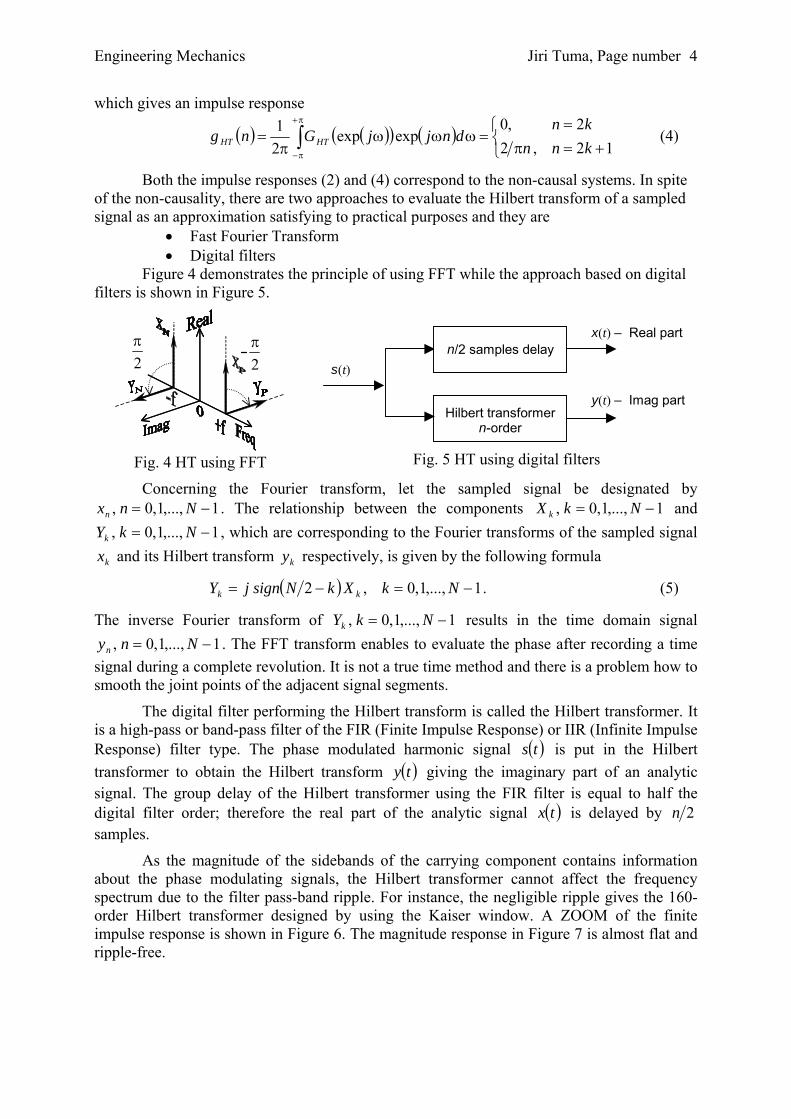
Both the impulse responses (2) and (4) correspond to the non-causal systems. In spite of the non-causality, there are two approaches to evaluate the Hilbert transform of a sampled signal as an approximation satisfying to practical purposes and they are

• Fast Fourier Transform • Digital filters

Figure 4 demonstrates the principle of using FFT while the approach based on digital filters is shown in Figure 5.

2 π

2 π

Fig. 4 HT using FFT

n/2 samples delay

Hilbert transformern-order

s (t)

x ( t ) – Real part

y ( t ) – Imag part

Fig. 5 HT using digital filters

Concerning the Fourier transform, let the sampled signal be designated by 1,...,1,0, −= Nnxn . The relationship between the components 1,...,1,0, −= NkX k and 1,...,1,0, −= NkYk , which are corresponding to the Fourier transforms of the sampled signal

kx and its Hilbert transform ky respectively, is given by the following formula

( ) 1,...,1,0,2 −=−= NkXkNsignjY kk . (5)

The inverse Fourier transform of 1,...,1,0, −= NkYk results in the time domain signal 1,...,1,0, −= Nnyn . The FFT transform enables to evaluate the phase after recording a time

signal during a complete revolution. It is not a true time method and there is a problem how to smooth the joint points of the adjacent signal segments.

The digital filter performing the Hilbert transform is called the Hilbert transformer. It is a high-pass or band-pass filter of the FIR (Finite Impulse Response) or IIR (Infinite Impulse Response) filter type. The phase modulated harmonic signal ( )ts is put in the Hilbert transformer to obtain the Hilbert transform ( )ty giving the imaginary part of an analytic signal. The group delay of the Hilbert transformer using the FIR filter is equal to half the digital filter order; therefore the real part of the analytic signal ( )tx is delayed by 2n samples.

As the magnitude of the sidebands of the carrying component contains information about the phase modulating signals, the Hilbert transformer cannot affect the frequency spectrum due to the filter pass-band ripple. For instance, the negligible ripple gives the 160-order Hilbert transformer designed by using the Kaiser window. A ZOOM of the finite impulse response is shown in Figure 6. The magnitude response in Figure 7 is almost flat and ripple-free.


5

Impulse Response : Hilbert Transformer - Order 160

-0,8-0,6-0,4-0,20,00,20,40,60,8

40 50 60 70 80 90 100 110 120

Index n

hH

T(n

)

Fig. 6 ZOOM of the impulse response (the 160-order FIR filter)

FIR Filter FRF : Hilbert Transformer - Order 160

0,0

0,2

0,4

0,6

0,8

1,0

1,2

0,0 0,2 0,4 0,6 0,8 1,0 1,2 1,4 1,6 1,8 2,0

Normalised Frequency f / f s [-]

|GH

T(f /

fs)

|

Fig. 7 Magnitude frequency response (the 160-order FIR filter)

Principle of the phase demodulation It is assumed that the angular vibration is measured by using encoders attached to the

shafts with the gears. The encoders produce usually a train of impulses, rather then a sinusoid. The frequency spectrum of the impulse signal consists of several harmonics of the basic impulse frequency. The first step in the phase demodulation procedure is to separate the frequency band containing a carrier component and adjacent sideband components by using a band-pass filter. Afterward, it is good to evaluate the Hilbert transform of a phase-modulated signal. An example of the phase-modulated signal composed only from the carrying frequency and adjacent sidebands is shown in Figure 8.

-1

0

1

0 0,1 0,2 0,3 0,4 0,5 0,6 0,7 0,8 0,9 1

Time [s]

s (t)

Fig. 8 Phase-modulated signal

The real and imaginary parts of the analytic signal, meaning the complex value nn yjx + , are inputs for evaluation the phase. The phase in the interval ( 2,2 ππ− can be

evaluated using the atan function ( )nnn xyatan=ϕ (6)


6

Signs of the real and imaginary part extend evaluation the phase on the interval ( ππ− , . The angle ranges from π− to π+ and contains jumps at π− at or π+ (see Figure 9).

The true phase nϕ of the analytical signal as the time function must be unwrapped. The unwrapping algorithm is based on the fact that the absolute value of the phase difference

1−ϕ−ϕ=ϕ∆ nnn between two consecutive samples of the phase is less than π

nnnnnn ϕ→π−ϕ⇒π+>ϕ∆ϕ→π+ϕ⇒π−<ϕ∆ 2,2 . (7)

2π

-4 -2 0 2 4

0 0.1 0.2 0.3 0.4 0.5 0.6 0.7 0.8 0.9 1 Time [s]

φ [ra

d]

+π

−π

Fig. 9 Phase of analytical signal ranging from –π to +π

The result of phase unwrapping of a phase-modulated harmonic signal is shown on the left diagram in Figure 10. The phase on this diagram is not a linear function of time, but an additive harmonic term to the linear term influences it. The unwrapped phase change per a second is equal to the angle π2 in radians, which is moreover multiplied by the number K of the modulated signal periods per a second. The number K is called the carrying frequency of the modulated signal. If the number of pulses generated per an encoder revolution is equal to K , the phase normalization has to be performed to evaluate a uniformity of rotation related to a complete revolution 1,...,1,0, −=ϕ→ϕ NnK nn . (8)

The phase normalization results in the phase scale that corresponds to an angle of a shaft rotation. The linear term of the normalized phase can determine the nominal phase corresponding to the uniform rotation. After removing the linear term from the actual phase as a time function in the left diagram of Figure 10, the phase modulation signal is obtained as it is seen on the right diagram in Figure 10.

0 1 2 3 4 5 6 7

0 0.2 0.4 0.6 0.8 1Time [s]

φ [ra

d]

-0.15-0.10-0.0500.050.100.15

0 0.2 0.4 0.6 0.8 1Time [s]

φ [ra

d]

Fig. 10 Unwrapped and removed linear trend in phase of analytical signal

Transmission error measurements The basic equation for evaluation TE of a simple gear set is given as

( ) 211

22 r

nnmTE ⎟⎟

⎠

⎞⎜⎜⎝

⎛Θ−Θ= , (9)


7

where 21, nn are teeth numbers of the pinion and wheel respectively, 21 ,ΘΘ are the angles of rotation of the mentioned gears and 2r is the wheel radius.

TE results not only from manufacturing inaccuracies, such as profile errors, tooth pitch errors and run-out, but from bad design. The pure tooth involute deflects under load due to the finite mesh stiffness. A gear case and shaft system deflects due to load as well.

The sketch of the gear set consisting of the 21- and 44-tooth gears under test and attached incremental rotary encoders, designated by E1 and E2, is shown in Figure 11. Both the encoders generate a string of impulses. As a consequence of Shannon’s sampling theorem a few impulses must be recorded during each mesh cycle. It means that the number of impulses produced per encoder complete revolution must be a multiple of the tooth number. If five harmonics of toothmeshing frequency are required to distinguish then the number of impulses per gear revolution must be at least ten

times greater than the number of teeth. The encoder generating 500 impulses per revolution seems to be an optimum.

As it was mentioned, a perfectly uniform rotation of gear produces an encoder signal having in its frequency spectrum a single component at the frequency that is a multiple of the gear rotational frequency and the number of teeth. The phase of this carrying component is a linear function of time. As the phase is the argument of the cosine function it can be associated with the gear rotation angle. The non-uniform rotation results in small variation of the rotation angle around the mentioned linear function of time. In this case the basic frequency of the impulse signal is modulated, which gives rise to sidebands around the carrying component in the frequency spectrum.

Using Fourier transform to evaluate Hilbert transform As it was mentioned, the Hilbert Transform can be evaluated by using either FFT or a

digital filter (Hilbert transformer). This chapter describes using of the first method. Before evaluating FFT it is recommended to resample the measured signal according to the gear rotational frequency in such a way that the length of resampled time record equals to a power of two, namely to at least 2048 samples per gear revolution for the 500-impulse encoder. The impulse signal order spectrum for the 2048-sample record ranges to the value of 800 orders. There is a space for ±300 sideband components around the carrying component of the 500-order component. The resampling of recorded signals is an obvious part so called order analyzers. Records are presented as a function of dimensionless revolutions rather than seconds and the corresponding FFT spectra are presented with the frequency axis dimensionless orders rather than frequency in Hz.

The order spectra of impulse string produced by encoders in Figure 11 are shown in Figure 12. The pinion is rotating at 500 RPM and under load of 40 Nm. Both these measurements were done by the same order analyzer and not simultaneously. For the first measurement the basic frequency for resampling was equal to the rotational speed of the pinion while at the second measurement resampling was done according to the rotation of the wheel.

The gear speed variation at the toothmeshing frequency results in the phase modulation of the impulse signal base frequency. As noted above the phase-modulated signal contains sideband components around the carrying component situated in Figure 12 at 500 ± 21k order for the 21-tooth pinion and at 500 ± 44k order for the 44-tooth wheel, where k =

Fig. 11 TE measurement arrangement


8

1,2,.. . Take notice of the fact that the dominating components in both the sideband families exceed the background noise level at least by 20 dB or even more. Both the spectra were evaluated from time signals that are a result of the synchronized averaging of 100 revolutions of gears under testing.

Enhanced Spectrum, 21-Tooth Gear

-90-80-70-60-50-40-30-20-10

010

395 416 437 458 479 500 521 542 563 584 605Order [-]

RM

S d

B /

ref 1

V

Enhanced Spectrum, 44-Tooth Gear

-90-80-70-60-50-40-30-20-10

010

324 368 412 456 500 544 588 632 676

Order [-]

RM

S d

B /

ref 1

VFig. 12 Frequency spectrum of phase modulated signal generated by the E1 and E2 encoders

Records corresponding to the complete rotation of the pinion and wheel are inputs for evaluation the Hilbert transform and unwrapped phase. The result for the 21-tooth gear is shown in Figure 13. The diagram time axis is in revolutions, which is in fact the dimensionless quantity τ related to the length of the time interval of one complete gear revolution. In other words, this dimensionless quantity τ is relative nominal rotation angle corresponding to the uniform rotation. The phase variation in Figure 13 is not normalized. Comparing both the diagrams shows the range of the uniformity rotation.

Pinion 21T : Unwrapped phase

0

30000

60000

90000

120000

150000

180000

0,0 0,2 0,4 0,6 0,8 1,0

Revolution τ [-]

500 Θ

1 [d

eg]

Pinion 21T : Phase modulating signal

-8-6-4-202468

1012

0,0 0,2 0,4 0,6 0,8 1,0

Revolution τ [-]

500 ∆Θ

1 [d

eg]

Fig. 13 Unwrapped phase and phase modulating signal (encoder E1)

The phase normalization gives the angles 500 times less (the encoder gives 500 impulses). The phase modulating signal related to the gear complete revolution is evaluated as the difference of the normalized unwrapped phase 1Θ and the linear term as the nominal rotation

τπ−Θ=∆Θ 211 , (10)

where τ is the normalized time corresponding to the pinion complete revolution. Low frequency oscillation dominates in the phase variation ( 1500∆Θ ) on the right diagram of Figure 13. The frequency spectra in the dB scale of both the phase variations ( 1∆Θ and 2∆Θ )


9

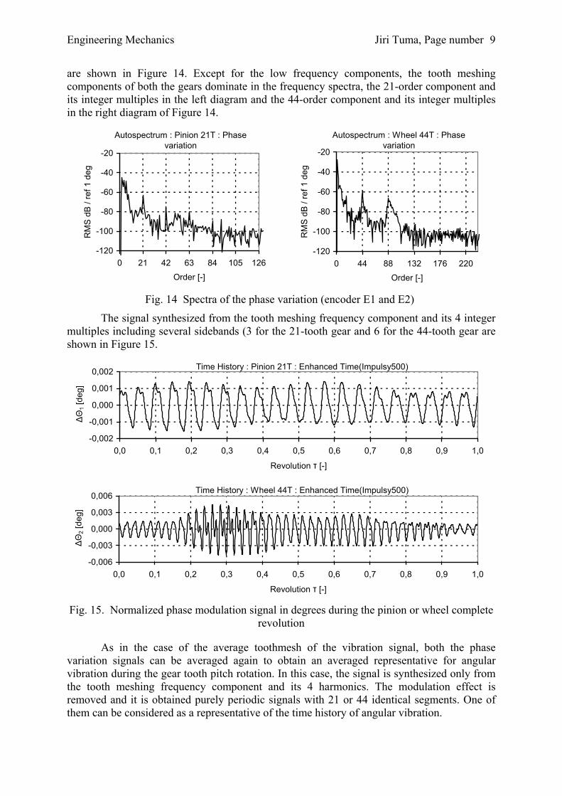
are shown in Figure 14. Except for the low frequency components, the tooth meshing components of both the gears dominate in the frequency spectra, the 21-order component and its integer multiples in the left diagram and the 44-order component and its integer multiples in the right diagram of Figure 14.

Autospectrum : Pinion 21T : Phase variation

-120

-100

-80

-60

-40

-20

0 21 42 63 84 105 126

Order [-]

RM

S d

B /

ref 1

deg

Autospectrum : Wheel 44T : Phase variation

-120

-100

-80

-60

-40

-20

0 44 88 132 176 220

Order [-]

RM

S d

B / r

ef 1

deg

Fig. 14 Spectra of the phase variation (encoder E1 and E2)

The signal synthesized from the tooth meshing frequency component and its 4 integer multiples including several sidebands (3 for the 21-tooth gear and 6 for the 44-tooth gear are shown in Figure 15.

Time History : Pinion 21T : Enhanced Time(Impulsy500)

-0,002

-0,001

0,000

0,001

0,002

0,0 0,1 0,2 0,3 0,4 0,5 0,6 0,7 0,8 0,9 1,0

Revolution τ [-]

∆Θ

1 [de

g]

Time History : Wheel 44T : Enhanced Time(Impulsy500)

-0,006

-0,003

0,000

0,003

0,006

0,0 0,1 0,2 0,3 0,4 0,5 0,6 0,7 0,8 0,9 1,0

Revolution τ [-]

∆Θ

2 [de

g]

Fig. 15. Normalized phase modulation signal in degrees during the pinion or wheel complete

revolution

As in the case of the average toothmesh of the vibration signal, both the phase variation signals can be averaged again to obtain an averaged representative for angular vibration during the gear tooth pitch rotation. In this case, the signal is synthesized only from the tooth meshing frequency component and its 4 harmonics. The modulation effect is removed and it is obtained purely periodic signals with 21 or 44 identical segments. One of them can be considered as a representative of the time history of angular vibration.


10

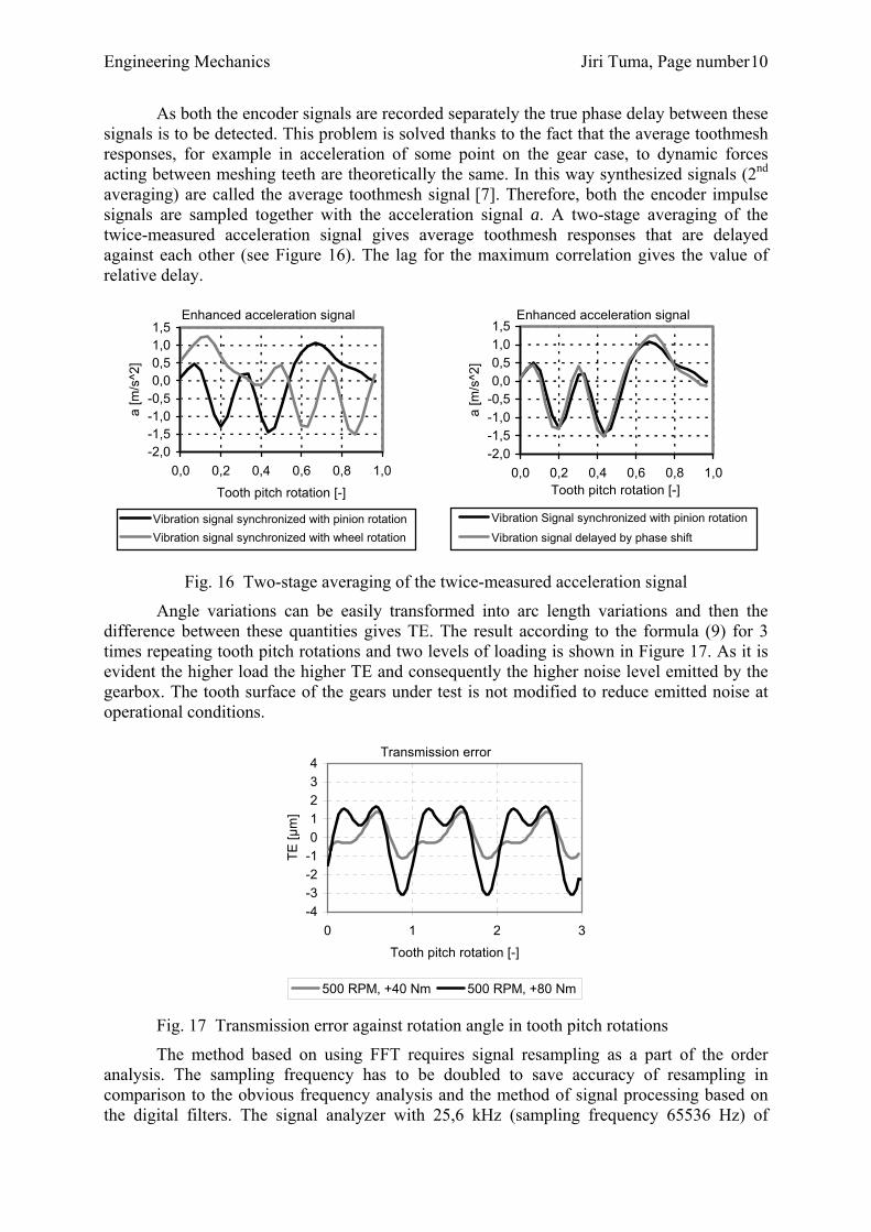
As both the encoder signals are recorded separately the true phase delay between these signals is to be detected. This problem is solved thanks to the fact that the average toothmesh responses, for example in acceleration of some point on the gear case, to dynamic forces acting between meshing teeth are theoretically the same. In this way synthesized signals (2nd averaging) are called the average toothmesh signal [7]. Therefore, both the encoder impulse signals are sampled together with the acceleration signal a. A two-stage averaging of the twice-measured acceleration signal gives average toothmesh responses that are delayed against each other (see Figure 16). The lag for the maximum correlation gives the value of relative delay.

Enhanced acceleration signal

-2,0-1,5-1,0-0,50,00,51,01,5

0,0 0,2 0,4 0,6 0,8 1,0

Tooth pitch rotation [-]

a [m

/s^2

]

Vibration signal synchronized with pinion rotation Vibration signal synchronized with wheel rotation

Enhanced acceleration signal

-2,0-1,5-1,0-0,50,00,51,01,5

0,0 0,2 0,4 0,6 0,8 1,0Tooth pitch rotation [-]

a [m

/s^2

]

Vibration Signal synchronized with pinion rotation

Vibration signal delayed by phase shift

Fig. 16 Two-stage averaging of the twice-measured acceleration signal

Angle variations can be easily transformed into arc length variations and then the difference between these quantities gives TE. The result according to the formula (9) for 3 times repeating tooth pitch rotations and two levels of loading is shown in Figure 17. As it is evident the higher load the higher TE and consequently the higher noise level emitted by the gearbox. The tooth surface of the gears under test is not modified to reduce emitted noise at operational conditions.

Transmission error

-4-3-2-101234

0 1 2 3

Tooth pitch rotation [-]

TE [µ

m]

500 RPM, +40 Nm 500 RPM, +80 Nm

Fig. 17 Transmission error against rotation angle in tooth pitch rotations

The method based on using FFT requires signal resampling as a part of the order analysis. The sampling frequency has to be doubled to save accuracy of resampling in comparison to the obvious frequency analysis and the method of signal processing based on the digital filters. The signal analyzer with 25,6 kHz (sampling frequency 65536 Hz) of


11

frequency range limits the RPM range of measurement to approximately 1900 RPM using the above described procedure.

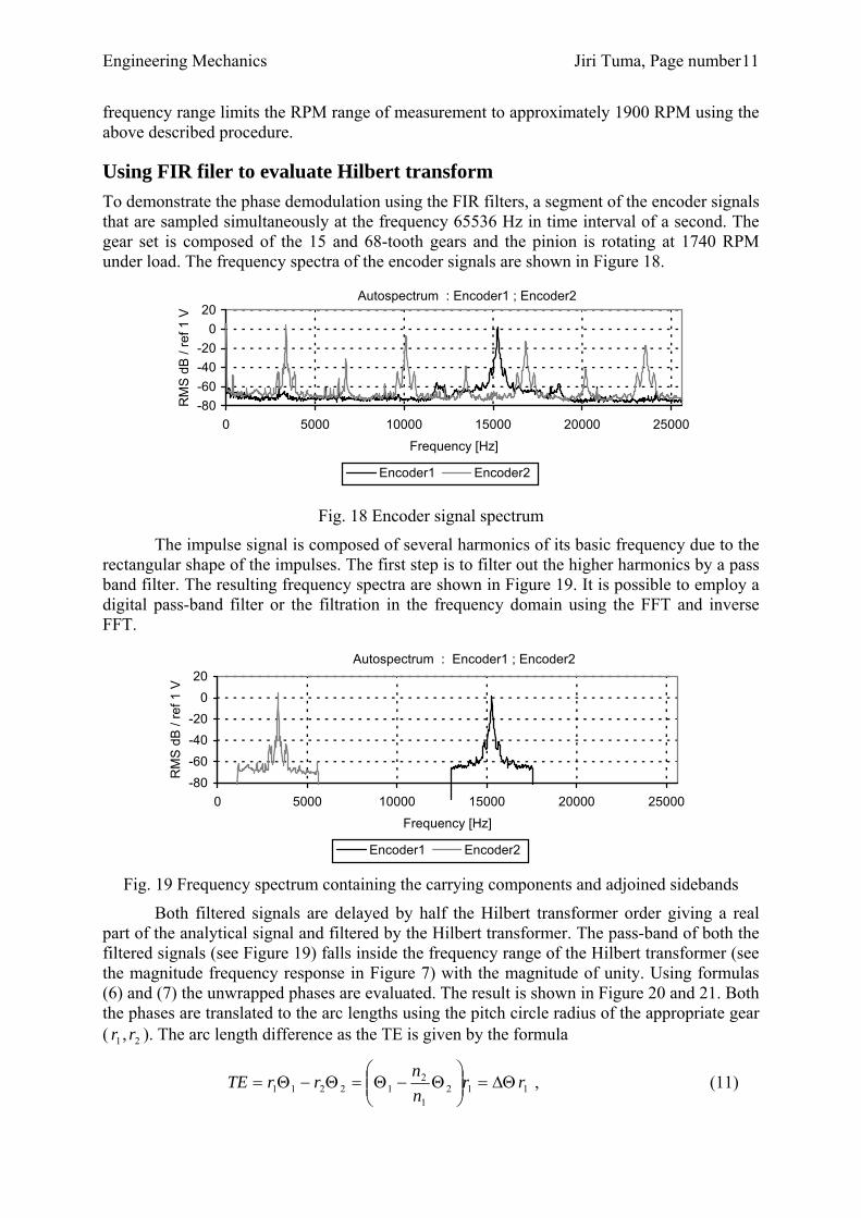
Using FIR filer to evaluate Hilbert transform To demonstrate the phase demodulation using the FIR filters, a segment of the encoder signals that are sampled simultaneously at the frequency 65536 Hz in time interval of a second. The gear set is composed of the 15 and 68-tooth gears and the pinion is rotating at 1740 RPM under load. The frequency spectra of the encoder signals are shown in Figure 18.

Autospectrum : Encoder1 ; Encoder2

-80-60-40-20

020

0 5000 10000 15000 20000 25000

Frequency [Hz]

RM

S d

B /

ref 1

V

Encoder1 Encoder2

Fig. 18 Encoder signal spectrum

The impulse signal is composed of several harmonics of its basic frequency due to the rectangular shape of the impulses. The first step is to filter out the higher harmonics by a pass band filter. The resulting frequency spectra are shown in Figure 19. It is possible to employ a digital pass-band filter or the filtration in the frequency domain using the FFT and inverse FFT.

Autospectrum : Encoder1 ; Encoder2

-80-60-40-20

020

0 5000 10000 15000 20000 25000

Frequency [Hz]

RM

S d

B /

ref 1

V

Encoder1 Encoder2

Fig. 19 Frequency spectrum containing the carrying components and adjoined sidebands

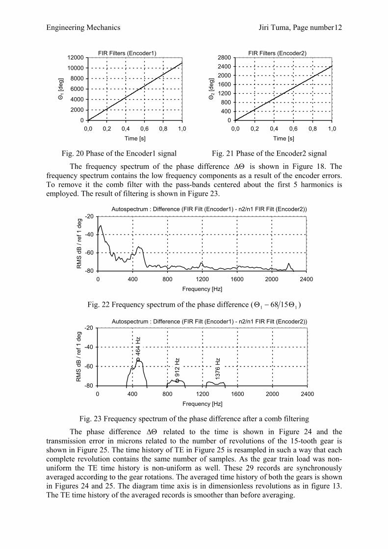
Both filtered signals are delayed by half the Hilbert transformer order giving a real part of the analytical signal and filtered by the Hilbert transformer. The pass-band of both the filtered signals (see Figure 19) falls inside the frequency range of the Hilbert transformer (see the magnitude frequency response in Figure 7) with the magnitude of unity. Using formulas (6) and (7) the unwrapped phases are evaluated. The result is shown in Figure 20 and 21. Both the phases are translated to the arc lengths using the pitch circle radius of the appropriate gear ( 21 , rr ). The arc length difference as the TE is given by the formula

1121

212211 rr

nn

rrTE ∆Θ=⎟⎟⎠

⎞⎜⎜⎝

⎛Θ−Θ=Θ−Θ= , (11)


12

FIR Filters (Encoder1)

0

2000

4000

6000

8000

10000

12000

0,0 0,2 0,4 0,6 0,8 1,0

Time [s]

Θ1 [

deg]

Fig. 20 Phase of the Encoder1 signal

FIR Filters (Encoder2)

0400800

12001600200024002800

0,0 0,2 0,4 0,6 0,8 1,0

Time [s]

Θ2 [

deg]

Fig. 21 Phase of the Encoder2 signal

The frequency spectrum of the phase difference ∆Θ is shown in Figure 18. The frequency spectrum contains the low frequency components as a result of the encoder errors. To remove it the comb filter with the pass-bands centered about the first 5 harmonics is employed. The result of filtering is shown in Figure 23.

Autospectrum : Difference (FIR Filt (Encoder1) - n2/n1 FIR Filt (Encoder2))

-80

-60

-40

-20

0 400 800 1200 1600 2000 2400Frequency [Hz]

RM

S d

B /

ref 1

deg

Fig. 22 Frequency spectrum of the phase difference ( 11 1568 Θ−Θ )

Autospectrum : Difference (FIR Filt (Encoder1) - n2/n1 FIR Filt (Encoder2))

464

Hz

912

Hz

1376

Hz

-80

-60

-40

-20

0 400 800 1200 1600 2000 2400

Frequency [Hz]

RM

S d

B /

ref 1

deg

Fig. 23 Frequency spectrum of the phase difference after a comb filtering

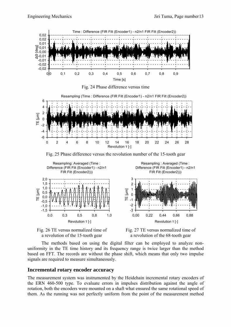
The phase difference ∆Θ related to the time is shown in Figure 24 and the transmission error in microns related to the number of revolutions of the 15-tooth gear is shown in Figure 25. The time history of TE in Figure 25 is resampled in such a way that each complete revolution contains the same number of samples. As the gear train load was non-uniform the TE time history is non-uniform as well. These 29 records are synchronously averaged according to the gear rotations. The averaged time history of both the gears is shown in Figures 24 and 25. The diagram time axis is in dimensionless revolutions as in figure 13. The TE time history of the averaged records is smoother than before averaging.


13

Time : Difference (FIR Filt (Encoder1) - n2/n1 FIR Filt (Encoder2))

-0,02-0,02-0,01-0,010,000,010,010,020,02

0,0 0,1 0,2 0,3 0,4 0,5 0,6 0,7 0,8 0,9

Time [s]

∆Θ

[deg

]

Fig. 24 Phase difference versus time

Resampling (Time : Difference (FIR Filt (Encoder1) - n2/n1 FIR Filt (Encoder2))

-6

-4

-2

0

2

4

6

0 2 4 6 8 10 12 14 16 18 20 22 24 26 28Revolution τ [-]

TE [µ

m]

Fig. 25 Phase difference versus the revolution number of the 15-tooth gear

Resampling: Averaged (Time : Difference (FIR Filt (Encoder1) - n2/n1

FIR Filt (Encoder2)))

-1,5-1,0-0,50,00,51,01,52,0

0,0 0,3 0,5 0,8 1,0

Revolution τ [-]

TE [µ

m]

Fig. 26 TE versus normalized time of

a revolution of the 15-tooth gear

Resampling : Averaged (Time : Difference (FIR Filt (Encoder1) - n2/n1

FIR Filt (Encoder2)))

-3-2-10123

0,00 0,22 0,44 0,66 0,88

Revolution τ [-]

TE [µ

m]

Fig. 27 TE versus normalized time of

a revolution of the 68-tooth gear

The methods based on using the digital filter can be employed to analyze non-uniformity in the TE time history and its frequency range is twice larger than the method based on FFT. The records are without the phase shift, which means that only two impulse signals are required to measure simultaneously.

Incremental rotary encoder accuracy The measurement system was instrumented by the Heidehain incremental rotary encoders of the ERN 460-500 type. To evaluate errors in impulses distribution against the angle of rotation, both the encoders were mounted on a shaft what ensured the same rotational speed of them. As the running was not perfectly uniform from the point of the measurement method


14

sensitivity, both the impulse signals were under the influence of phase modulation due to the errors in impulses positions versus the angle rotation. Using the analytical method described above, the difference between modulation signals gives the error in impulse distribution. The frequency spectrum of the resulting error is shown in Figure 28. The frequency axis is in orders and both the axes are logarithmic. The error spectrum components in the RMS level corresponds to the rotation angle of orderπ2 in radians. The error level corresponding to the tooth pitch rotation determines the final accuracy of the T.E. measurement. As it is evident the magnitude of an error at 21 and 44 order is less than 10-5 radians, i.e. approximately 2 angular seconds. The error corresponding to the 15 and 68 order is at least by an order lower than the TE for this gear train. Measurement accuracy is satisfactory.

The total error of the rotational angle over the arbitrary number of adjacent impulses is given by the sum of individual errors corresponding to the rotation by an impulse. The summation process results in the error spectrum, which can be approximated in logarithmic scale by a strait line. The spectrum roll-off is such that decreasing the RMS by a decade corresponds to increasing the order by a decade as well. This property is confirmed by Figure 28.

Phase difference

0,000001

0,000010

0,000100

0,001000

0,010000

0,100000

1,000000

1 10 100 1000Order [-]

Err

or R

MS

[deg

]

634 RPM1040 RPME1E2 E1E2

1/Order

Fig. 28 Spectrum of the phase difference for 634 and 1040 RPM

Conclusion This paper is focused on the problem of the simple gear set transmission error measurement (T.E.). Variation of TE is the cause of angular vibration of both the mating gears and consequently gearcase vibration and noise. This paper deals with only one measurement method that is based on the use of encoders generating a string of 500 impulses per gear revolution. The impulse signal is processed by the Hilbert transform using the FFT or the digital filter. The advantages and disadvantages of both these methods are discussed. Employing the FFT for evaluation the Hilbert transform gives the TE time history only for a tooth pitch rotation while employing the digital filter results in the TE time history of several gear complete rotations and the RPM range is twice larger than for the previously mentioned method. The theory is illustrated by experimental data.


15

Bibliography

[1] D.B. Welbourn, Fundamental knowledge of gear noise – A survey, In: Proceedings Noise & Vib. Of. Eng. And Trans., I Mech E, --14, (1979).

[2] Ch-H. Chung, G. Steyer, T. Abe, M. Clapper, Ch. Shah, Gear Noise Reduction through Transmission Error Control and Gear Blank Dynamic Tuning, SAE Paper 1999-01-1766.

[3] M. Hortel, A. Škuderová, K analýze lineárního a nelineárního tlumení v převodových soustavách s rázy, In: Inženýrská mechanika. Stockholm, May 9-12, 2005.

[4] Z. Dejl, V. Moravec V. Modification of Spur Involute Gearing. In: The Eleventh World Congress on Mechanism and Machine Science, Tianjin, China, April 1-4, 2004, pp. 782-786.

[5] J. Tuma, Phase Demodulation of Impulse Signals in Machine Shaft Angular Vibration Measurements. In: Proceedings of Tenth international congress on sound and vibration (ICSV10). Stockholm, July 7-10, 2003, pp. 5005-5012.

[6] D. J. Smith, Gear Noise and Vibration, 1st ed., Marcel Dekker Inc., New York and Basel 1999.

[7] J. Tuma, R. Kubena, V. Nykl, Assessment of Gear Quality Considering the Time Domain Analysis of Noise and Vibration Signals. In: Proceedings of 1994 Gear International Conference. Newcastle, September 1994, pp.463-468.

[8] M. Henriksson and M. Pärssinen, Comparison of Gear Noise and Dynamic Transmission Error Measurements. In: Proceedings of Tenth international congress on sound and vibration (ICSV10). Stockholm, July 7-10, 2003, pp. 4005-4012.

This research has been done at the Department of Control Systems and Instrumentation as a part of the research project No. 101/04/1530 and has been supported by the Czech Grant Agency.

dynamic transmission error measurementshomel.vsb.cz/~tum52/publications/te_measurements.pdf · an...

Documents