dynamic voltage scaling techniques for power...

Dynamic Voltage Scaling Techniques forPower Efficient Video Decoding

Ben Lee‡, Eriko Nurvitadhi‡, Reshma Dixit‡, Chansu Yu†, and Myungchul Kim*,

‡School of Electrical Engineering and Computer ScienceOregon State University

Corvallis, OR 97331{benl, nurviter, dixit}@eecs.orst.edu

†Department of Electrical and Computer EngineeringCleveland State UniversityCleveland, OH 44115-2425

[email protected]

*School of EngineeringInformation and Communications University

58-4 Hwa-am, Yu-sung, Taejon, 305-348 [email protected]

AbstractThis paper presents a comparison of power-aware video decoding techniques that utilize DynamicVoltage Scaling (DVS) capability. These techniques reduce the power consumption of a processor byexploiting high frame variability within a video stream. This is done through scaling of the voltage andfrequency of the processor during the video decoding process. However, DVS causes frame deadlinemisses due to inaccuracies in decoding time predictions and granularity of processor settings used. Fourtechniques were simulated and compared in terms of power consumption, accuracy, and deadline misses.We propose the Frame-data Computation Aware (FDCA) technique, which is a useful power-savingtechnique not only for stored video but also for real-time video applications. We compare this techniquewith the GOP, Direct, and Dynamic methods, which tend to be more suited for stored video applications.The simulation results indicated that the Dynamic per-frame technique, where the decoding timeprediction adapts to the particular video being decoded, provides the most power saving with aperformance comparable to the ideal case. On the other hand, the FDCA method consumes more powerthan the Dynamic method but can be used for stored video and real-time time video scenarios without theneed for any preprocessing. Our findings also indicate that in general power savings increase, but thenumber of deadline misses also increase as the number of processor settings used in a DVS algorithm areincreased. More importantly, most of these deadline misses are within 10%-20% of the playout intervaland thus insignificant. However, video clips with high variability in frame complexities combined withinaccurate decoding time predictions may degrade the video quality. Finally, our results show that aprocessor with 13 voltage/frequency settings should be sufficient to achieve near maximum performancewith the experimental environment and the video workloads we have used.

Keywords: Dynamic voltage scaling, video decoding, low-power techniques, decoding time prediction.

1. Introduction

Power efficient design is one of the most important goals for mobile devices, such as laptops, PDAs,

handhelds, and mobile phones. As the popularity of multimedia applications for these portable devices

increases, reducing their power consumption will become increasingly important. Among multimedia

applications, delivering video will become the most challenging and important applications of future

mobile devices. Video conferencing and multimedia broadcasting are already becoming more common,

especially in conjunction with the Third Generation (3G) wireless network initiative [11]. However,

video decoding is a computationally intensive, power ravenous process. In addition, due to different

frame types and variation between scenes, there is a great degree of variance in processing requirements

during execution. For example, the variance in per-frame MPEG decoding time for the movie Terminator

2 can be as much as a factor of three [1], and the number of Inverse Discrete Cosine Transforms (IDCTs)

performed for each frame varies between 0 and 2000 [7]. This high variability in video streams can be

exploited to reduce power consumption of the processor during video decoding.

Dynamic Voltage Scaling (DVS) has been shown to take advantage of the high variability in

processing requirements by varying the processor’s operating voltage and frequency during run-time [4,

10]. In particular, DVS is suitable for eliminating idle times during low workload periods. Recently,

researchers have attempted to apply DVS to video decoding to reduce power [18, 17, 21, 19, 24, 33].

These studies present approaches that predict the decoding times of incoming frames or Group of Pictures

(GOPs), and reduce or increase the processor setting based on this prediction. As a result, idle processing

time, which occurs when a specific frame decoding completes earlier than its playout time, is minimized.

In an ideal case, the decoding times are estimated perfectly, and all the frames (or GOPs) are decoded at

the exact time span allowed. Thus, there is no power wasted by an idle processor waiting for a frame to

be played. In practice, decoding time estimation leads to errors that result in frames being decoded either

before or after their playout time. When the decoding finishes early, the processor will be idle while it

waits for the frame to be played, and some power will be wasted. When decoding finishes late, the frame

will miss its playout time, and the perceptual quality of the video could be reduced.

Even if decoding time prediction is very accurate, the maximum DVS performance can be

achieved only if the processor can scale to very precise processor settings. Unfortunately, such a

processor design is impractical since there is cost associated with having different processor supply

voltages. Moreover, the granularity of voltage/frequency settings induces a tradeoff between power

savings and deadline misses. For example, fine-grain processor settings may even increase the number of

deadline misses when it is used with an inaccurate decoding time predictor. Coarse-grain processor

settings, on the other hand, lead to overestimation by having voltage and frequency set a bit higher than

required. This reduces deadline misses in spite of prediction errors, but at the cost of reduced power

savings. Therefore, the impact of processor settings on video decoding with DVS needs to be further

investigated.

Based on the aforementioned discussion, this paper provides a comparative study of the existing

DVS techniques developed for low-power video decoding, such as Dynamic [33], GOP [21], and Direct

[18, 24], with respect to prediction accuracy and the corresponding impact on performance. These

approaches are designed to perform well even with a high-motion video by either using static prediction

model or dynamically adapting its prediction model based on the decoding experience of the particular

video clip being played. However, they also require video streams to be preprocessed to obtain the

necessary parameters for the DVS algorithm, such as frame sizes, frame-size/decoding-time relationship,

or both. To overcome this limitation, this paper also proposes an alternative method called Frame-data

Computation Aware (FDCA) method. FDCA dynamically extracts useful frame characteristics while a

frame is being decoded and uses this information to estimate the decoding time. Extensive simulation

study based on SimpleScalar processor model [5], Wattch power tool [3] and Berkeley MPEG Player [2]

has been conducted to compare these DVS approaches.

Our focus is to investigate two important tradeoffs: The impact of decoding time predictions and

granularity of processor settings on DVS performance in terms of power savings, playout accuracy, and

characteristics of deadline misses. To the best of our knowledge, a comprehensive study that provides

such a comparison has not been performed, yet such information is critical to better understand the notion

of applying DVS for low-power video decoding. For example, existing methods only use a specific

number of processor settings and thus do not provide any guidelines on an appropriate granularity of

processor settings when designing DVS techniques for video decoding. Moreover, these studies

quantified the DVS performance by only looking at power savings and the number of deadline misses. In

this paper, we further expose the impact of deadline misses by measuring the extent to which the deadline

misses exceed the desired playout time.

The rest of the paper is organized as follows. Section 2 presents a background on DVS. Section

3 introduces the existing and proposed DVS techniques on low-power video decoding and discusses their

decoding time predictors. Section 4 discusses the simulation environment and characteristics of video

streams used in this study. It also presents the simulation results on how the accuracy of decoding time

predictor and the granularity of processor settings affect DVS performance. Finally, Section 5 provides a

conclusion and elaborates on future work.

2. Background on Dynamic Voltage Scaling (DVS)

DVS has been proposed as a mean for a processor to deliver high performance when required, while

significantly reducing power consumption during low workload periods [4, 9, 10, 12-24, 33]. The

advantage of DVS can be observed from the power consumption characteristics of digital static CMOS

circuits [21] and the clock frequency equation [24]:

CLKDDeff fVCP 2∝ (1)

( )21

TDD

DD

CLK VV

V

f −∝∝τ (2)

where Ceff is the effective switching capacitance, VDD is the supply voltage, fCLK is the clock frequency, τ

is the circuit delay that bounds the upper limit of the clock frequency, and VT is the threshold voltage.

Decreasing the power supply voltage would reduce power consumption significantly (Equation 1).

However, it would lead to higher propagation delay, and thus force a reduction in clock frequency

(Equation 2). While it is generally desirable to have the frequency as high as possible for faster

instruction execution, for some tasks where maximum execution speed is not required, the clock

frequency and supply voltage can be reduced so that power can be saved.

DVS takes advantage of this tradeoff between energy and speed. Since processor activity is

variable, there are idle periods when no useful work is being performed, yet power is still consumed.

DVS can be used to eliminate these power-wasting idle times by lowering the processor’s voltage and

frequency during low workload periods so that the processor will have meaningful work at all times,

which leads to reduction in the overall power consumption.

However, the difficulty in applying DVS lies in the estimation of future workload. For example,

Pering et al. took into account the global state of the system to determine the most appropriate scaling for

the future [23], but the performance benefit is limited because the estimation at the system level is not

generally accurate. Another work by Pering and Brodersen considers the characteristics of individual

threads without differentiating their behavior [22]. Flautner et al. classifies each thread by their

communication characteristics to well known system tasks, such as X server or the sound daemon [9].

Lorch and Smith assign pre-deadline and post-deadline periods for each task and gradually accelerate the

speed in between these periods [15]. While these approaches apply DVS at the Operating System level,

for some types of applications that inhibit high variability in their execution, such as video decoders,

greater power saving can be achieved if DVS is incorporated into the application itself. The next section

overviews existing DVS approaches for low-power video decoding.

3. Prediction-based DVS Approaches for Low-Power Video Decoding

This section introduces various DVS approaches for low-power video decoding. They utilize some form

of a decoding time prediction algorithm to dynamically perform voltage scaling [18, 17, 21, 24, 32, 33].

In Subsection 3.1, we show how the low-power video decoding benefits from DVS and how the accuracy

of decoding time predictor affects the performance of DVS. Subsection 3.2 describes three existing DVS

approaches and the proposed FDCA approach with a focus on prediction algorithms. In Subsection 3.3,

the impact of the granularity of the processor settings on DVS performance is discussed.

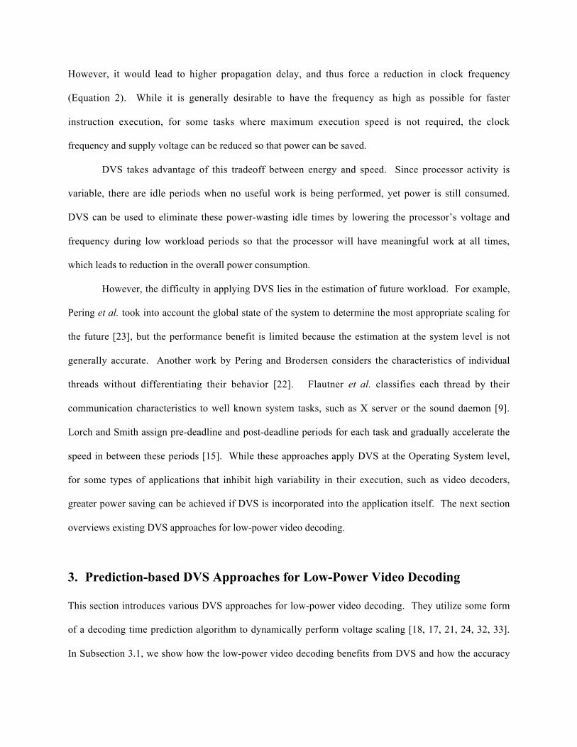
3.1 Prediction Accuracy on DVS Performance

Figure 1 illustrates the advantage of DVS in video decoding as well as the design tradeoff between

prediction accuracy, power savings, and deadline misses. The processor speed on the y-axes directly

relates to voltage as discussed earlier, and reducing the speed allows the reduction in supply voltage,

which in turn results in power savings. The shaded area corresponds to the work required to decode the

four frames and it is the same in all three cases. However, the corresponding power consumption is the

largest in Figure 1a because it uses the highest voltage/frequency setting and there is a quadratic

relationship between the supply voltage and power consumption (see Equation 1 in Section 2).

Figure 1a shows the processor activity when DVS is not used, which means that the processor

runs at a constant speed (in this case at 120 MHz). Once a frame is decoded, the processor waits until

(e.g., every 33.3 ms for the frame rate of 30 frames per second or fps) when the frame must be played out.

During this idle period, the processor is still running and consuming power. These idle periods are the

target for exploitation by DVS. Figure 1b shows the ideal case where the processor scales exactly to the

voltage/frequency setting required for the desired time span. Therefore, no idle time exists and power

saving is maximized. Achieving this goal involves two important steps. First, the decoding time must be

predicted. Second, the predicted decoding time must be mapped to an appropriate voltage/frequency

setting.

Inaccurate predictions in decoding time and/or use of insufficient number of voltage/frequency

settings will introduce errors that lead to reduction in power saving and/or increase in missed deadlines as

shown in Figure 1c. In this figure, the decoding times for frames 1 and 4 are overestimated, resulting in

more power consumption than required. On the other hand, the decoding time for frame 2 is

underestimated, which leads to a deadline miss that may degrade the video quality. In summary, DVS has

great potential in applications with high varying workload intensities such as video decoding, but accurate

workload prediction is prerequisite in realizing the benefit of DVS.

Frame 1Frame

2

Frame3

Frame4

130

230

330

430

CPU speed(Mhz)

Time(sec)

120

Frame 1 isdisplayed

Frame 2 isdisplayed

Frame 3 isdisplayed

Frame 4 isdisplayed

100

80

60

40

CPU decodes frame

(a) Without DVS.

Frame 1Frame 2 Frame 3 Frame 4

130

230

330

430

CPU speed(Mhz)

Time(sec)

120

Frame 1 isdisplayed

Frame 2 isdisplayed

Frame 3 isdisplayed

Frame 4 isdisplayed

100

80

60

40

(b) With DVS (Ideal)


130

230

330

430

CPU speed(Mhz)

Time(sec)

120

Frame 1 isdisplayed

Frame 2 isdisplayed

Frame 3 isdisplayed

Frame 4 isdisplayed

100

80

60

40

(c) Prediction inaccuracies.

Figure 1: Illustration of DVS.

3.2 Overview of DVS Approaches and Their Prediction Schemes

As clearly shown in Figure 1, an accurate prediction algorithm is essential to improve DVS performance

and to maintain video quality. Prediction algorithms employed in several DVS approaches differ based

on the following two criteria: prediction interval and prediction mechanism. Prediction interval refers to

how often predictions are made in order to apply DVS. The existing approaches use either per-frame or

per-GOP scaling. In per-GOP approaches, since the same voltage/frequency is used while decoding a

particular GOP, they do not take full advantage of the high variability of decoding times among frames

within a GOP.

Prediction mechanism refers to the way the decoding time of an incoming frame or GOP is

estimated. Currently, all the approaches utilize some form of frame size vs. decoding time relationship

[1]. Some methods are based on a fixed relationship, while others use a dynamically changing

relationship. In the fixed approach, a linear equation describing the relationship between frame sizes and

frame decoding times is provided ahead of time. In the dynamic approach, the frame-size/decoding-time

relationship is dynamically adjusted based on the actual frame-related data and decoding times of a video

stream being played. The dynamic approach is better for high-motion videos where the workload

variability is extremely high. In other cases, the fixed approach performs better than the dynamic

approach but its practical value is limited because the relationship is not usually available before actually

decoding the stream.

Aside from the two criteria explained above, the DVS schemes are classified as either off-line or

on-line. A DVS scheme is classified as on-line if no preprocessing is required to obtain information to be

used in the DVS algorithm and therefore is equally adaptable for stored video and real-time video

applications. It is classified as off-line if preprocessing is required to obtain information needed by the

DVS algorithm.

Four DVS techniques for video decoding and the corresponding prediction algorithms are

discussed and compared: GOP is a per-GOP, dynamic off-line approach, Direct is a per-frame, fixed off-

line approach, while Dynamic and FDCA are per-frame, dynamic approaches with Dynamic being an off-

line scheme and FDCA being an on-line scheme. Intuitively, GOP consumes more energy and incurs

more deadline misses than Direct and Dynamic but would result in the least overhead because the

prediction interval is longer. Direct would perform the best because it is based on a priori information on

decoding times and their relationship with the corresponding frame sizes. It should be noted that the

offline methods have one striking drawback in that they all require a priori knowledge of encoded frame

sizes and therefore, need some sort of preprocessing. There is also a method that completely bypasses the

decoding time prediction at the client to eliminate the possibilities of errors due to inaccurate scaling

predictions [17]. This is done by preprocessing video streams off-line on media servers to add accurate

video complexity information during the encoding process. However, this approach requires knowledge

of client hardware and is therefore impractical. Moreover, it is not useful in case of existing streams that

may not include the video complexity information. Choi et al. [32] have proposed a method in which the

frame is divided into a frame-dependent and frame-independent part and scale voltage accordingly.

However, as mentioned in their work, it is possible for errors to propagate across frames due to a single

inaccurate prediction, thereby degrading video quality. We do not include these two methods in the

study.

3.2.1 Per-GOP Approach with Dynamic Equation (GOP)

GOP is a per-GOP scaling approach that dynamically recalculates the slope of the frame-size/decode-time

relationship based on the decoding times and sizes of past frames [21]. At the beginning of a GOP, the

sizes and types of the frames of an incoming GOP are observed. This information is then applied to the

frame-size/decode-time model, and the time needed to decode the GOP is estimated. Based on this

estimate, the lowest frequency and voltage setting that would satisfy the frame rate requirement is

selected. The dynamic slope adjustment was originally presented in [1]. Here, the slope adjustment is

implemented by utilizing the concept of Decoding Time Per Byte (DTPB). DTPB essentially represents

the slope of the frame-size/decode-time equation and this value is updated as the video is decoded using

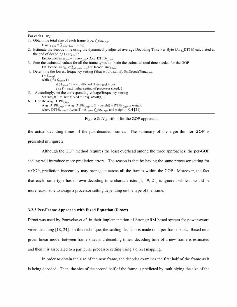
the actual decoding times of the just-decoded frames. The summary of the algorithm for GOP is

presented in Figure 2.

Although the GOP method requires the least overhead among the three approaches, the per-GOP

scaling will introduce more prediction errors. The reason is that by having the same processor setting for

a GOP, prediction inaccuracy may propagate across all the frames within the GOP. Moreover, the fact

that each frame type has its own decoding time characteristic [1, 19, 21] is ignored while it would be

more reasonable to assign a processor setting depending on the type of the frame.

3.2.2 Per-Frame Approach with Fixed Equation (Direct)

Direct was used by Pouwelse et al. in their implementation of StrongARM based system for power-aware

video decoding [18, 24]. In this technique, the scaling decision is made on a per-frame basis. Based on a

given linear model between frame sizes and decoding times, decoding time of a new frame is estimated

and then it is associated to a particular processor setting using a direct mapping.

In order to obtain the size of the new frame, the decoder examines the first half of the frame as it

is being decoded. Then, the size of the second half of the frame is predicted by multiplying the size of the

For each GOPi:1. Obtain the total size of each frame type, f_sizef_type

f_sizef_type = ∑each f_type f_sizei;2. Estimate the decode time using the dynamically adjusted average Decoding Time Per Byte (Avg_DTPB) calculated at

the end of decoding GOPi-1, i.e.,EstDecodeTimef_type= f_sizef_type× Avg_DTPBf_type;

3. Sum the estimated values for all the frame types to obtain the estimated total time needed for the GOPEstDecodeTimeGOPi=∑all frame types EstDecodeTimef_type;

4. Determine the lowest frequency setting f that would satisfy EstDecodeTimeGOPi.f = flowest;while ( f ≤ fhighest ) {

if ( flowest / fps ≥ EstDecodeTimeGOPi) break;else f = next higher setting of processor speed; }

5. Accordingly, set the corresponding voltage/frequency settingSetFreq(f) { MHz = f; Vdd = FreqToVolt(f); }

6. Update Avg_DTPBf_type:Avg_DTPBf_type = Avg_DTPBf_type x (1 - weight) + DTPBf_type x weight,where DTPBf_type = ActualTimef_type / f_sizef_type and weight = 0.4 [21].

Figure 2: Algorithm for the GOP approach.

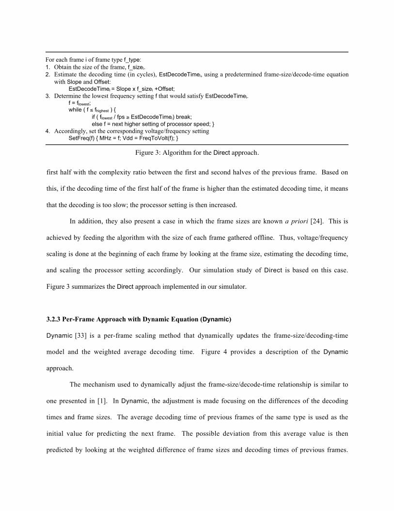
first half with the complexity ratio between the first and second halves of the previous frame. Based on

this, if the decoding time of the first half of the frame is higher than the estimated decoding time, it means

that the decoding is too slow; the processor setting is then increased.

In addition, they also present a case in which the frame sizes are known a priori [24]. This is

achieved by feeding the algorithm with the size of each frame gathered offline. Thus, voltage/frequency

scaling is done at the beginning of each frame by looking at the frame size, estimating the decoding time,

and scaling the processor setting accordingly. Our simulation study of Direct is based on this case.

Figure 3 summarizes the Direct approach implemented in our simulator.

3.2.3 Per-Frame Approach with Dynamic Equation (Dynamic)

Dynamic [33] is a per-frame scaling method that dynamically updates the frame-size/decoding-time

model and the weighted average decoding time. Figure 4 provides a description of the Dynamic

approach.

The mechanism used to dynamically adjust the frame-size/decode-time relationship is similar to

one presented in [1]. In Dynamic, the adjustment is made focusing on the differences of the decoding

times and frame sizes. The average decoding time of previous frames of the same type is used as the

initial value for predicting the next frame. The possible deviation from this average value is then

predicted by looking at the weighted difference of frame sizes and decoding times of previous frames.

For each frame i of frame type f_type:1. Obtain the size of the frame, f_sizei.2. Estimate the decoding time (in cycles), EstDecodeTimei, using a predetermined frame-size/decode-time equation

with Slope and Offset:EstDecodeTimei = Slope x f_sizei +Offset;

3. Determine the lowest frequency setting f that would satisfy EstDecodeTimei.f = flowest;while ( f ≤ fhighest ) {

if ( flowest / fps ≥ EstDecodeTimei) break;else f = next higher setting of processor speed; }

4. Accordingly, set the corresponding voltage/frequency settingSetFreq(f) { MHz = f; Vdd = FreqToVolt(f); }

Figure 3: Algorithm for the Direct approach.

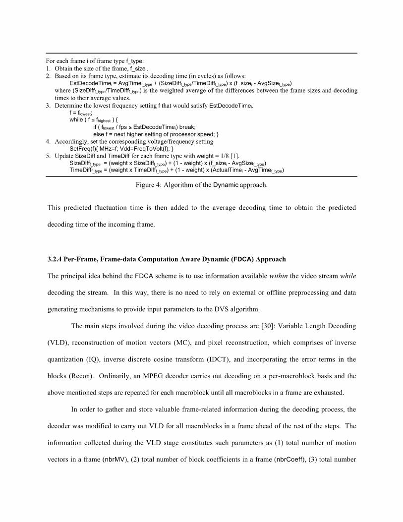
This predicted fluctuation time is then added to the average decoding time to obtain the predicted

decoding time of the incoming frame.

3.2.4 Per-Frame, Frame-data Computation Aware Dynamic (FDCA) Approach

The principal idea behind the FDCA scheme is to use information available within the video stream while

decoding the stream. In this way, there is no need to rely on external or offline preprocessing and data

generating mechanisms to provide input parameters to the DVS algorithm.

The main steps involved during the video decoding process are [30]: Variable Length Decoding

(VLD), reconstruction of motion vectors (MC), and pixel reconstruction, which comprises of inverse

quantization (IQ), inverse discrete cosine transform (IDCT), and incorporating the error terms in the

blocks (Recon). Ordinarily, an MPEG decoder carries out decoding on a per-macroblock basis and the

above mentioned steps are repeated for each macroblock until all macroblocks in a frame are exhausted.

In order to gather and store valuable frame-related information during the decoding process, the

decoder was modified to carry out VLD for all macroblocks in a frame ahead of the rest of the steps. The

information collected during the VLD stage constitutes such parameters as (1) total number of motion

vectors in a frame (nbrMV), (2) total number of block coefficients in a frame (nbrCoeff), (3) total number

For each frame i of frame type f_type:1. Obtain the size of the frame, f_sizei.2. Based on its frame type, estimate its decoding time (in cycles) as follows:

EstDecodeTimei = AvgTimef_type + (SizeDifff_type/TimeDifff_type) x (f_sizei - AvgSizef_type)where (SizeDifff_type/TimeDifff_type) is the weighted average of the differences between the frame sizes and decodingtimes to their average values.

3. Determine the lowest frequency setting f that would satisfy EstDecodeTimei.f = flowest;while ( f ≤ fhighest ) {

if ( flowest / fps ≥ EstDecodeTimei) break;else f = next higher setting of processor speed; }

4. Accordingly, set the corresponding voltage/frequency settingSetFreq(f){ MHz=f; Vdd=FreqToVolt(f); }

5. Update SizeDiff and TimeDiff for each frame type with weight = 1/8 [1].SizeDifff_type = (weight x SizeDifff_type) + (1 - weight) x (f_sizei - AvgSizef_type)TimeDifff_type = (weight x TimeDifff_type) + (1 - weight) x (ActualTimei - AvgTimef_type)

Figure 4: Algorithm of the Dynamic approach.

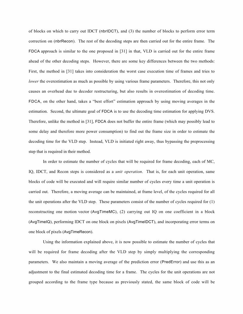
of blocks on which to carry out IDCT (nbrIDCT), and (3) the number of blocks to perform error term

correction on (nbrRecon). The rest of the decoding steps are then carried out for the entire frame. The

FDCA approach is similar to the one proposed in [31] in that, VLD is carried out for the entire frame

ahead of the other decoding steps. However, there are some key differences between the two methods:

First, the method in [31] takes into consideration the worst case execution time of frames and tries to

lower the overestimation as much as possible by using various frame parameters. Therefore, this not only

causes an overhead due to decoder restructuring, but also results in overestimation of decoding time.

FDCA, on the other hand, takes a “best effort” estimation approach by using moving averages in the

estimation. Second, the ultimate goal of FDCA is to use the decoding time estimation for applying DVS.

Therefore, unlike the method in [31], FDCA does not buffer the entire frame (which may possibly lead to

some delay and therefore more power consumption) to find out the frame size in order to estimate the

decoding time for the VLD step. Instead, VLD is initiated right away, thus bypassing the preprocessing

step that is required in their method.

In order to estimate the number of cycles that will be required for frame decoding, each of MC,

IQ, IDCT, and Recon steps is considered as a unit operation. That is, for each unit operation, same

blocks of code will be executed and will require similar number of cycles every time a unit operation is

carried out. Therefore, a moving average can be maintained, at frame level, of the cycles required for all

the unit operations after the VLD step. These parameters consist of the number of cycles required for (1)

reconstructing one motion vector (AvgTimeMC), (2) carrying out IQ on one coefficient in a block

(AvgTimeIQ), performing IDCT on one block on pixels (AvgTimeIDCT), and incorporating error terms on

one block of pixels (AvgTimeRecon).

Using the information explained above, it is now possible to estimate the number of cycles that

will be required for frame decoding after the VLD step by simply multiplying the corresponding

parameters. We also maintain a moving average of the prediction error (PredError) and use this as an

adjustment to the final estimated decoding time for a frame. The cycles for the unit operations are not

grouped according to the frame type because as previously stated, the same block of code will be

executed regardless of the type of the frame. The error terms however, are grouped depending on the

frame type. The estimated number of cycles for a frame is then used to apply DVS by selecting the

lowest frequency/voltage setting that would meet the frame deadline. The VLD step is performed at the

highest voltage/frequency available to leave as much time as possible to perform DVS during the more

computationally intensive tasks after VLD. Figure 5 gives an algorithmic description of the FDCA

scheme.

3.3 Granularity of Processor Settings on DVS Performance

In this subsection, the impact of granularity of processor settings on DVS performance is discussed.

Figure 6a is the same ideal DVS approach as in Figure 1b. It is ideal not only because the decoding time

prediction is prefect but also because the processor can be set precisely to any voltage/frequency value.

Unfortunately, a processor design with a large number of voltage/frequency scales is unfeasible [6, 13],

since there is some cost involved in having different processor supply voltages [25, 27]. For this reason,

DVS capable commercial processors typically employ a fixed number of voltage and frequency settings.

For each frame i of frame type f_type:1. Perform VLD at the highest voltage/frequency setting available and obtain nbrMV, nbrCoeff, nbrIDCT, and

nbrRecon.2. At the end of VLD, determine the time available (tRemaining) and estimate the time (in cycles) required for all the

decoding steps after VLD using data gathered in Step 1 above and Step 5 below.EstDecodeTimei = (nbrMVi × AvgTimeMC) + (nbrCoeffi × AvgTimeIQ) + (nbrIDCTi × AvgTimeIDCT) +

(nbrReconi × AvgTimeRecon) + (PredErrorf_type)3. Determine the lowest frequency setting f that would satisfy EstDecodeTimei

f = flowest;while ( f ≤ fhighest ) {

if ((EstDecodeTimei / f) < tRemaining) break;else f = next higher setting of processor speed; }

4. Accordingly, set the corresponding voltage/frequency setting.SetFreq(f){ MHz=f; Vdd=FreqToVolt(f); }

5. Update AvgTimeMC, AvgTimeIQ, AvgTimeIDCT, AvgTimeRecon, and PredErrorf_type (Window size= n):AvgTimeMCi = ActualTimeMCi / nbrMVi and AvgTimeMCi+1 = ∑last n frames AvgTimeMC / nAvgTimeIQi = ActualTimeIQi / nbrCoeffi and AvgTimeIQi+1 = ∑last n frames AvgTimeIQ / nAvgTimeIDCTi = ActualTimeIDCTi / nbrIDCTi and AvgTimeIDCTi+1 = ∑last n frames AvgTimeIDCT / nAvgTimeReconi = ActualTimeReconi / nbrReconi and AvgTimeReconi+1 = ∑last 5 frames AvgTimeRecon / nPredErrorf_type = EstDecodeTimei - ActualTimeIQi and PredErrori+1 = ∑last n frames PredError / n

Figure 5: Algorithm of the FDCA approach.

For example, Transmeta TM5400 or “Crusoe” processor has 6 voltage scales ranging from 1.1 V to 1.65

V with frequency settings of 200 MHz to 700 MHz [24], while Intel StrongARM SA-100 has up to 13

voltage scales from 0.79 V to 1.65 V with the frequency settings of 59 MHz to 251 MHz [10].

Consider a processor that has a fixed scale of frequencies, e.g., 5 settings ranging from 40 MHz to

120 MHz with steps of 20 MHz as in Figure 6b. The closest available frequency that can still satisfy the

deadline requirement is selected by DVS algorithm. In Figure 6c, the scales used in the previous case are

halved, which results in 9 frequency scales with steps of 10 MHz. This results in less idle times than the


130

230

330

430

CPU speed(Mhz)

Time(sec)

120

Frame 1 isdisplayed

Frame 2 isdisplayed

Frame 3 isdisplayed

Frame 4 isdisplayed

100

80

60

40

(a) With DVS (Ideal)

Frame 1Frame 2

Frame 3 Frame 4

130

230

330

430

CPU speed(Mhz)

Time(sec)

120

Frame 1 isdisplayed

Frame 2 isdisplayed

Frame 3 isdisplayed

Frame 4 isdisplayed

100

80

60

40

(b) Coarse-grain scales.


130

230

330

430

CPU speed(Mhz)

Time(sec)

120

Frame 1 isdisplayed

Frame 2 isdisplayed

Frame 3 isdisplayed

Frame 4 isdisplayed

100

80

60

40

110

90

70

50

(c) Fine-grain scales.

Figure 6: Granularity of scales.

previous case and more power saving is achieved. If finer granularity scales than Figure 6c are used,

power savings would improve until at some point when it reaches the maximum as in the ideal case.

Nevertheless, more frame deadline misses will also start to occur as finer granularity scales are used with

inaccuracies in predicting decoding times. That is, prediction errors together with use of fine-grain

settings would introduce more deadline misses. On the other hand, use of coarse-grain settings induces

overestimation that could avoid deadline misses in spite of prediction errors. Thus, it is important to

understand which level of voltage scaling granularity in a DVS algorithm is fine enough to give

significant power savings and minimize deadline misses, while still reasonably coarse to be implemented.

4. Performance Evaluation and Discussions

In this section, we present the simulation results comparing different DVS schemes introduced in Section

3.2, and also show the quantitative results on the effect of the granularity of processor settings on DVS

performance in Section 3.3. Performance measures are average power consumption per frame, error rate,

and deadline misses. Before proceeding, the simulation environment and the workload video streams are

first described in Subsections 4.1 and 4.2, respectively.

4.1 Simulation Environment

Figure 7 shows our simulation environment, which consists of modified SimpleScalar [5], Wattch [3], and

Berkeley mpeg_play MPEG-1 Decoder [2]. SimpleScalar [5] is used as the basis of our simulation

framework. The simulator is configured to resemble the characteristics of a five-stage pipeline

architecture, which is typical of processors used in current portable multimedia devices. The proxy

system call handler in SimpleScalar was modified and a system call for handling voltage and frequency

scaling was added. Thus, the MPEG decoder makes a DVS system call to the simulator to adjust the

processor setting.

Wattch [3] is an extension to the SimpleScalar framework for analyzing power consumption of

the processor. It takes into account the simulator’s states and computes the power consumption of each of

the processor structures as the simulation progresses. The power parameters in Wattch contain the values

of the power consumption for each hardware structure at a given cycle time. Thus, by constantly

observing these parameters, our simulator is capable of obtaining the power used by the processor during

decoding of each frame.

The Berkeley mpeg_play MPEG-1 decoder [2] was used as the video decoder in our simulation

environment. For the FDCA scheme, the original decoder was restructured to carry out VLD ahead of the

other steps in video decoding. All the methods required modifications of the decoder to make DVS

system calls to the simulator. A DVS system call modifies the voltage and frequency values presently

used by SimpleScalar. These system calls are also used to find out the number of cycles required for

decoding a frame and updating data used in an algorithm during the decoding process. In the GOP,

Direct, and Dynamic methods, there are two system calls made: One at the start of a frame and one at the

end of a frame. In the FDCA method, there are also other system calls made to update data related to

cycles for unit operations.

For the simulation study, the overhead of processor scaling was assumed to be negligible. In

practice, there is a little overhead related with the scaling. Previously implemented DVS systems have

shown that processor scaling takes about 70 µs to 140 µs [4, 18, 24]. Since this overhead is significantly

CBenchmark Source

MPEG decoder

SimpleScalarGCC

SimpleScalarExecutable File

Compiler Option

sim-outorderPerformance

Simulator

WattchPower Estimator

Hardware Configuration

SimpleScalar

Performance Statistics

Total Power consumption

MPEG stream

CBenchmark Source

MPEG decoder

SimpleScalarGCC

SimpleScalarExecutable File

Compiler Option

sim-outorderPerformance

Simulator

WattchPower Estimator

Hardware Configuration

SimpleScalar

Performance Statistics

Total Power consumption

MPEG streamMPEG stream

Figure 7: Simulation environment.

smaller than the granularity at which the DVS system calls are made, they would have negligible affect on

the overall results.

4.2 Workload Video Streams

Three MPEG clips were used in our simulations. These clips were chosen as representatives of three

types of videos - low-motion, animation, and high-motion. A clip showing a public message on childcare

is selected for a low-motion video (Children) and a clip named Red’s Nightmare is selected as an

animation video. Lastly, a clip from the action movie Under Siege is selected to represent a high-motion

video. Table 1 shows the characteristics of the clips. The table also includes frame-size/decode-time

equations, which were generated after preprocessing each clip. The R2 coefficient represents the accuracy

of the linear equations, i.e., the closer R2 is to unity, the more likely the data points will lie on the

predicted line.

Figure 8 shows the decoding time characteristics for each of the clips. As expected, frame

decoding times for Under Siege fluctuate greatly, while the fluctuations in decoding times for Children

are very subtle and the separation of the decoding times for the three types of frames can be clearly seen.

For Red’s Nightmare, decoding times for I-frames are relatively unvarying, but P-frames show large

variations and B-frames are distinguished by peaks.

Table 1: The characteristics of the clips used in the simulation.Characteristics Children Red’s Nightmare Under Siege

Type Slow (Low-motion) Animation Action (High-motion)Frame Rate (fps) 29.97 25 30

Number of I frames 62 41 123Number of P frames 238 81 122Number of B frames 599 1089 486

Total number of frames 899 1211 731Screen size (W×H) 320 x 240 pixels 320 x 240 pixels 352 x 240 pixels

Linear equationfor prediction

Decoding time =88.8 × Frame size + 106

Decoding time =53.9 × Frame size + 2×106

Decoding time =69.6 × Frame size + 2×106

R2 coefficient 0.94 0.89 0.94

4.3 Effect of Prediction Accuracy on DVS Performance

Figures 9 and 10 summarize power savings and error results for the four DVS approaches simulated

(GOP, Dynamic, Direct, and FDCA). These simulations were carried out using 13-voltage/frequency

settings as used in the Intel StrongARM processor [18]. The ideal case (Ideal) was also included as a

reference. The ideal case represents perfect prediction with voltage/frequency set to any accuracy

Children

0

5

10

15

20

25

0 100 200 300 400 500 600 700 800

Frame Number

Dec

odin

g T

ime

(ms)

I Frames

P Frames

B Frames

Red's Nightmare

05

101520253035404550

0 200 400 600 800 1000 1200

Frame Number

Dec

odin

g T

ime

(ms)

I Frames

P Frames

B Frames

Under Siege

0

5

10

15

20

25

30

0 100 200 300 400 500 600 700

Frame Number

Dec

ode

Tim

e (m

s)

I frames

P frames

B Frames

Figure 8: Frame decoding times for each clip.

required, and thus represents optimum DVS performance. This was done by using previously gathered

actual frame decoding times to make scaling decisions instead of the estimated decoding times.

Figure 9 shows the power savings in terms of average power consumption per frame relative to

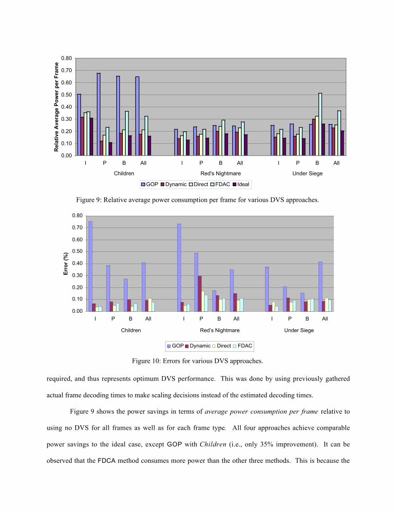
using no DVS for all frames as well as for each frame type. All four approaches achieve comparable

power savings to the ideal case, except GOP with Children (i.e., only 35% improvement). It can be

observed that the FDCA method consumes more power than the other three methods. This is because the

0.00

0.10

0.20

0.30

0.40

0.50

0.60

0.70

0.80

I P B All I P B All I P B All

Children Red's Nightmare Under Siege

Rel

ativ

e A

vera

ge

Po

wer

per

Fra

me

GOP Dynamic Direct FDAC Ideal

Figure 9: Relative average power consumption per frame for various DVS approaches.

0.00

0.10

0.20

0.30

0.40

0.50

0.60

0.70

0.80


Children Red’s Nightmare Under Siege

Err

or

(%)

GOP Dynamic Direct FDAC

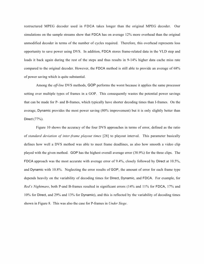
Figure 10: Errors for various DVS approaches.

restructured MPEG decoder used in FDCA takes longer than the original MPEG decoder. Our

simulations on the sample streams show that FDCA has on average 12% more overhead than the original

unmodified decoder in terms of the number of cycles required. Therefore, this overhead represents loss

opportunity to save power using DVS. In addition, FDCA stores frame-related data in the VLD step and

loads it back again during the rest of the steps and thus results in 9-14% higher data cache miss rate

compared to the original decoder. However, the FDCA method is still able to provide an average of 68%

of power saving which is quite substantial.

Among the off-line DVS methods, GOP performs the worst because it applies the same processor

setting over multiple types of frames in a GOP. This consequently wastes the potential power savings

that can be made for P- and B-frames, which typically have shorter decoding times than I-frames. On the

average, Dynamic provides the most power saving (80% improvement) but it is only slightly better than

Direct (77%).

Figure 10 shows the accuracy of the four DVS approaches in terms of error, defined as the ratio

of standard deviation of inter-frame playout times [28] to playout interval. This parameter basically

defines how well a DVS method was able to meet frame deadlines, as also how smooth a video clip

played with the given method. GOP has the highest overall average error (38.9%) for the three clips. The

FDCA approach was the most accurate with average error of 9.4%, closely followed by Direct at 10.5%,

and Dynamic with 10.8%. Neglecting the error results of GOP, the amount of error for each frame type

depends heavily on the variability of decoding times for Direct, Dynamic, and FDCA. For example, for

Red’s Nightmare, both P-and B-frames resulted in significant errors (14% and 11% for FDCA, 17% and

10% for Direct, and 29% and 13% for Dynamic), and this is reflected by the variability of decoding times

shown in Figure 8. This was also the case for P-frames in Under Siege.

4.4 Impact of Processor Settings Granularity

The results of power consumption and accuracy presented in the previous subsection were based on 13

frequency/voltage settings. Thus, even if very accurate decoding time predictions are made, the

granularity of voltage/frequency settings will invariably affect the performance of DVS. It seems that

having fine-grain voltage scales would lead to better performance than having coarse-grain scales.

Nevertheless, a clearer understanding is needed about the impact that various processor voltage/frequency

scaling granularities have on video decoding in terms of power consumption and accuracy.

To show the aforementioned tradeoff, we experimented with various scaling schemes consisting

of 4, 7, 13, 25, and 49 scales. Table 2 presents the voltage/frequency scaling schemes simulated. Each of

these schemes was simulated using the Dynamic as well as the FDCA approach. These approaches were

chosen as representatives among others due to their promising performance and high potential for realistic

implementation.

The results are shown in Figures 11-14. Figure 11 shows the relative average power consumption

per frame compared to using no DVS for various voltage/frequency processor settings for the Dynamic

method. As can be seen, power consumption decreases as the number of processor settings increase.

However, power saving only increases slightly beyond 13 scales. Thus, using 13 available settings seems

to be sufficient to achieve relative average power per frame comparable to the ideal case (e.g., 18% vs.

16% for Children, 19% vs. 17% for Red’s Nightmare, and 23% vs. 20% for Under Siege, respectively).

The results for the FDCA method are shown in Figure 13 and a similar trend of only a marginal increase

Table 2: Processor settings simulated.Voltages (V) Frequencies (MHz)

Number of SettingsRange Steps Range Steps

4 scales 0.286668 647 scales 0.143334 3213 scales 0.071667 1625 scales 0.035834 849 scales

0.79 to 1.65

0.017917

59 to 251

4Ideal Scale to any requested value by the ideal prediction algorithm

in power savings beyond 13 scales can also be observed with this method.

Figures 12 and 14 show the accuracy of the DVS approaches for the various settings for Dynamic

and FDCA techniques respectively. In general, the error decreases with the availability of more processor

settings. This is true for Children and Under Siege, where changing the available number of processor

settings from 4 to 49 settings significantly reduces the error. However, this is not the case for Red’s

Nightmare, the error decreases for the processor settings of 4 to 13. For the number of settings more than

0.00

0.05

0.10

0.15

0.20

0.25

0.30

0.35

0.40

0.45



Rel

ativ

e A

vera

ge

Po

wer

per

Fra

me

4 scales 7 scales 13 scales 25 scales 49 scales Ideal

Figure 11: Relative average power per frame for various processor settings for Dynamic method.

0.00

0.05

0.10

0.15

0.20

0.25

0.30

0.35



Err

or

(%)

4 scales 7 scales 13 scales 25 scales 49 scales

Figure 12: Errors for various processor settings for Dynamic method.

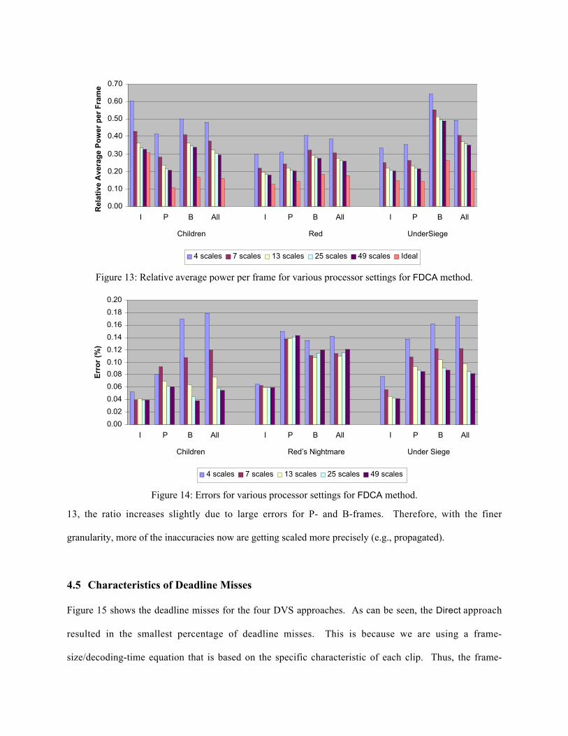
13, the ratio increases slightly due to large errors for P- and B-frames. Therefore, with the finer

granularity, more of the inaccuracies now are getting scaled more precisely (e.g., propagated).

4.5 Characteristics of Deadline Misses

Figure 15 shows the deadline misses for the four DVS approaches. As can be seen, the Direct approach

resulted in the smallest percentage of deadline misses. This is because we are using a frame-

size/decoding-time equation that is based on the specific characteristic of each clip. Thus, the frame-

0.00

0.10

0.20

0.30

0.40

0.50

0.60

0.70


Children Red UnderSiege

Rel

ativ

e A

vera

ge

Po

wer

per

Fra

me

4 scales 7 scales 13 scales 25 scales 49 scales Ideal

Figure 13: Relative average power per frame for various processor settings for FDCA method.

0.00

0.02

0.04

0.06

0.08

0.10

0.12

0.14

0.16

0.18

0.20



Err

or

(%)


Figure 14: Errors for various processor settings for FDCA method.

size/decoding-time model is well suited for the particular clip being run. For Direct, the Under Siege clip

resulted in the most number of misses (7.8%). The reason is that the clip is a high-motion video, which

deviates most from the calculated linear model.

However, the Dynamic and FDCA approaches handle the Under Siege clip comparatively well

(8.4% and 9.7% deadline misses respectively) because of their adaptive capability in predicting decoding

times. The Children clip resulted in the most number of misses (23.92%) for Dynamic, where the FDCA

method gave good results with 16.2% deadline misses. Even though P-frames for Children for FDCA

cause about 35% deadline misses, it is found that the deadline is missed only by an average of about 5%

and is therefore negligible. The highest number of deadline misses in Dynamic occurred for the clip with

the least amount of scene variations. This is because the dynamic decoding time estimation used

performs too aggressively for the clip that has smooth movement. GOP also uses an adaptive mechanism

similar to the Dynamic approach. However, the deadline misses are minimized by having longer scaling

intervals (i.e., per-GOP instead of per-frame). Moreover, its scaling decision includes all types of frames.

Thus, P- and B-frames, which typically have shorter decoding times than I-frames, would likely be

overestimated since the setting used has to also satisfy the playout times for I-frames.

0

20

40

60

80

100

120



Dea

dlin

e M

isse

s (%

)


Figure 15: Percentage of deadline misses for various DVS approaches.

Figures 16 and 17 show the deadline misses for various voltage/frequency scales using Dynamic

and FDCA respectively. The number of deadline misses increases linearly as the granularity of the

processor settings becomes finer, except for the Children clip in case of Dynamic. This is because by

using more number of settings, the scaling decisions rely more on the estimation of the decoding times.

Thus, an estimation error would easily propagate to cause a deadline miss. Essentially, the main factor

that would affect the relationship between the granularity of the processor scale and DVS performance is

0

5

10

15

20

25

30

35

40



Dea

dlin

e M

isse

s (%

)


Figure 16: Percentage of the deadlines misses for different processor settings for Dynamic.

0

10

20

30

40

50

60

70

80



Dea

dlin

e M

isse

s (%

)


Figure 17: Percentage of the deadlines misses for different processor settings for FDCA.

the distribution of the frame decoding times. The power savings and deadline misses would depend on

whether the processor settings available and used in the algorithm could satisfy the expansion of the

decoding times to the frame playout intervals.

Figure 18 show the characteristics of deadline misses in terms of how much the desired playout

times were exceeded for various DVS approaches. The x-axis shows the extent of the deadlines misses

relative to the playout interval, categorized as 10%, 20%, 30%, 40%, and greater than 40%. The y-axis

represents the percentage of deadline misses over an entire clip. For example, a 5% value on the y-axis

with the 10% category on x-axis means that 5% of the frames in the clip that miss the deadline missed it

by 10% of the desired playout interval (e.g., for 25 fps, or 40 ms playout interval, these frames are played

out between 40 to 44 ms after the preceding frames). For the Direct, Dynamic, and FDCA approaches,

most of the misses are within 10% of the playout interval. In addition, virtually all of the misses for the

above three approaches lie within the 20% range. In contrast, the deadline misses for GOP are more

erratic, and thus, have a higher potential of disrupting the quality of video playback. Conversely, deadline

misses in Direct, Dynamic, and FDCA are less likely to affect the quality of the videos.

0

5

10

15

20

25

<10%

<20%

<30%

<40%

>40%

<10%

<20%

<30%

<40%

>40%

<10%

<20%

<30%

<40%

>40%

<10%

<20%

<30%

<40%

>40%



Figure 18: The degree of deadline misses for various DVS approaches.

Based on these results, we can clearly see that the number of deadline misses by itself is not an

accurate measure of video quality. Instead, how much the desired playout times were exceeded should

also be measured and analyzed in order to provide a better understanding on how the misses may affect

the quality of video. The simulation results indicate that deadline misses imposed by DVS for most part

have negligible effect on perceptual quality since they are mostly within 10% after the desired playout

time [8].

5. Conclusion

This paper compared DVS techniques for low-power video decoding. Out of the four approaches studied,

Dynamic and Direct provided the most power savings, but are limited in usefulness with respect to real-

time video applications. The FDCA method can be effectively applied to both stored video and real-time

video applications. Due to the extra overhead required for restructuring the decoding process, FDCA does

not provide as much power savings as compared to the Dynamic and Direct methods. Nevertheless, the

power savings obtained is quite substantial providing up to an average of 68% savings and an average of

less than 14% (13.4%) frames missing the deadline. Thus, this approach is very suitable for portable

multimedia devices, which require low-power consumption.

Our study also further quantified the deadline misses that occurred by looking at the degree to

which the playout times are exceeded. The results indicate that, for the Dynamic, Direct, and FDCA

approaches, most of the deadline misses are within 20% of the playback interval. Therefore, use of these

power saving methods is less likely to degrade the quality of the video. In addition, in designing a DVS

capable processor for video decoding, higher number of processor settings is preferable. By using more

available settings, more power saving can be achieved without any additional risk of sacrificing quality of

the video. More deadline misses may occur, but they are still within a tolerable range [8].

As future work, it would be interesting to investigate the usage of DVS system on streaming

video where packet jitters from the network also need to be considered. It would also be useful to assess

the cost of implementing very fine-grain scales on a DVS processor. Finding more accurate prediction

mechanisms for unit operations in video decoding, in particular for IDCT, and new ways to exploit DVS

for low power video decoding is also critical and would assist in reaching near-maximum performance.

Finally, it would be beneficial to find ways to use DVS on other parts of a system, such as applying DVS

to memory or network interface.

6. References[1] A. Bavier, B. Montz, and L. Peterson, “Predicting MPEG Execution Times,” International

Conference on Measurement and Modeling of Computer Systems, pp. 131-140, June 1998.[2] Berkeley MPEG Tools. http://bmrc.berkeley.edu/frame/research/mpeg/[3] D. Brooks, V. Tiwari, and M. Martonosi, “Wattch: A Framework for Architectural-Level Power

Analysis and Optimizations”, Proc. of the 27th International Symposium on Computer Architecture,pp. 83-94, June 2000.

[4] T.D. Burd, T. A. Perimg, A. J. Stratakos, and R.W. Brodersen, “A Dynamic Voltage ScaledMicroprocessor System”, IEEE Journal of Solid-State Circuits, November 2000.

[5] D. Burger and T. M. Austin, “The SimpleScalar Tool Set, Version 2.0,” CSD Technical Report#1342, University of Wisconsin, Madison, June 1997.

[6] A. P. Chandrakasan, and R. W. Brodersen, “Low Power Digital CMOS Design,” Kluwer AcademicPublishers, 1995.

[7] A. Chandrakasan, V. Gutnik, T. Xanthopoulos, “Data Driven Signal Processing: An Approach forEnergy Efficient Computing,” Proc. of IEEE International Symposium on Low Power Electronicsand Design, pp.347-352, 1996.

[8] M. Claypool and J. Tanner, “The Effects of Jitter on the Perceptual Quality of Video,” Proc. of theACM Multimedia Conference, Vol. 2, November 1999.

[9] K. Flautner, S. Reinhardt, and T. Mudge, “Automatic Performance Setting for Dynamic VoltageScaling”, Proc. of the 17th Conference on Mobile Computing and Networking, July 2001.

[10] K. Govil, E. Chan, and H. Wasserman, “Comparing Algorithms for Dynamic Speed-Setting of aLow Power CPU,” Proc. 1st Int’l Conference on Mobile Computing and Networking, Nov 1995.

[11] L. Harte, R. Levine, and R. Kikta, “3G Wireless Demystified,” McGraw-Hill, 2002.[12] C. Im, H. Kim, and S. Ha, “Dynamic Voltage Scheduling Techniques for Low-Power Multimedia

Applications Using Buffers,” International Symposium on Low Power Electronics and Design(ISLPED ‘01), California, August 2001.

[13] T. Ishihara, and H. Yasuura, “Voltage Scheduling Problem for Dynamically Variable VoltageProcessors”, International Symposium on Low Power Electronics and Design, August 1998.

[14] S. Lee and T. Sakurai, “Run-time power control scheme using software feedback loop for low-powerreal-time applications,” Asia and South Pacific Design Automation Conference, January 2000.

[15] J. R. Lorch, and A. J. Smith, “Improving Dynamic Voltage Scaling Algorithms with PACE,” Proc.of the International Conference on Measurement and Modeling of Computer Systems, June 2001.

[16] D. Marculescu, “On the Use of Microarchitecture-Driven Dynamic Voltage Scaling,” Workshop onComplexity-Effective Design, held in conjunction with 27th International Symposium on ComputerArchitecture, June 2000.

[17] M. Mesarina and Y. Turner, “Reduced Energy Decoding of MPEG Streams,” ACM/SPIEMultimedia Computing and Networking 2002 (MMCN ’02), January 2002.

[18] J. Pouwelse, K. Langendoen, R. Lagendijk, and H. Sips, “Power-Aware Video Decoding, ” PictureCoding Symposium (PCS ’01), April 2001.

[19] J. Shin, “Real Time Content Based Dynamic Voltage Scaling”, Master Thesis, Information andCommunication University, Korea, January, 2002.

[20] T. Simunic, L. Benini, A. Acquaviva, P. Glynn, and G. D. Michelli, “Dynamic Voltage Scaling andPower Management for Portable Systems”, 38th Design Automation Conference (DAC 2001), June2001.

[21] D. Son, C. Yu, and H. Kim, “Dynamic Voltage Scaling on MPEG Decoding”, InternationalConference of Parallel and Distributed System (ICPADS), June 2001.

[22] T. Pering ,and R. Brodersen, “Energy Efficient Voltage Scheduling for Real-Time OperatingSystems”, In Proceedings of the 4th IEEE Real-Time Technology and Applications SymposiumRTAS'98, Work in Progress Session, June 1998.

[23] T. Pering, T. Burd, and R. Brodersen, “The Simulation and Evaluation of Dynamic Voltage ScalingAlgorithms”, Proc. of the International Symposium on Low Power Electronics and Design, August10-12, 1998.

[24] J. Pouwelse, K. Langendoen, and H. Sips, “Dynamic Voltage Scaling on a Low-PowerMicroprocessor,” 7th ACM Int. Conf. on Mobile Computing and Networking (Mobicom), July 2001.

[25] J. M. Rabaey, and M. Pedram, “Low Power Design Methodologies,” Kluwer Academic Publishers,1996.

[26] R. Steinmetz, “Human Perception of Jitter and Media Synchronization,” IEEE Journal on selectedAreas in Communications, Vol. 14, No. 1, January 1996.

[27] A. J. Stratakos, C. R. Sullivan, S. R. Sanders, and R.W. Brodersen, “High-Efficiency Low-VoltageDC-DC Conversion for Portable Applications,” Low-Voltage/Low-Power Integrated Circuits andSystems: Low Voltage Mixed-Signal Circuits, Edgar Sanchez-Sinencio and Andreas Andreou, Eds.IEEE Press, 1999.

[28] Y. Wang, M. Claypool, and Z. Zuo, “An Empirical Study of RealVideo Performance Across theInternet,” Proc. of the First Internet Measurement Workshop, pp. 295-309, November 2001.

[29] H. Zhang and S. Keshav, “Comparison of rate-based service disciplines,” Proc. of ACMSIGCOMM’91, Sept 1991.

[30] K. Patel, B. Smith and L.Rowe, “Performance of a Software MPEG Video Decoder,” Proc. of theFirst ACM International Conference on Multimedia, pp. 75-82, August 1993.

[31] L. O. Burchard and P. Altenbernd, “Estimating Decoding Times of MPEG-2 Video Streams,”Proceedings of International Conference on Image Processing (ICIP 00), 2000.

[32] K. Choi, K. Dantu, W.-C.Chen, and M. Pedram, “Frame-Based Dynamic Voltage and FrequencyScaling for a MPEG Decoder,” Proc. of International Conference on Computer Aided Design(ICCAD), 2002.

[33] E. Nurvitadhi, B. Lee, C. Yu, and M. Kim, “A Comparative Study of Dynamic Voltage ScalingTechniques for Low-Power Video Decoding,” International Conference on Embedded Systems andApplications, June 23-26 2003.

dynamic voltage scaling techniques for power...

Documents