This article was downloaded by: [University of Sheffield]On: 20 January 2015, At: 00:58Publisher: Taylor & FrancisInforma Ltd Registered in England and Wales Registered Number: 1072954 Registered office: Mortimer House,37-41 Mortimer Street, London W1T 3JH, UK

Click for updates

Systems Science & Control Engineering: An OpenAccess JournalPublication details, including instructions for authors and subscription information:http://www.tandfonline.com/loi/tssc20

Dynamically dual vibration absorbers: a bond graphapproach to vibration controlPeter Gawthropa, S.A. Neildb & D.J. Waggc

a Systems Biology Laboratory, Melbourne School of Engineering, University of Melbourne,Victoria 3010, Australiab Department of Mechanical Engineering, Queens Building, University of Bristol, Bristol BS81TR., UKc Department of Mechanical Engineering, Sir Frederick Mappin Building, University ofSheffield, Mappin Street Sheffield S1 3JD, UKAccepted author version posted online: 01 Dec 2014.Published online: 14 Jan 2015.

To cite this article: Peter Gawthrop, S.A. Neild & D.J. Wagg (2015) Dynamically dual vibration absorbers: a bond graphapproach to vibration control, Systems Science & Control Engineering: An Open Access Journal, 3:1, 113-128, DOI:10.1080/21642583.2014.991458

To link to this article: http://dx.doi.org/10.1080/21642583.2014.991458

PLEASE SCROLL DOWN FOR ARTICLE

Taylor & Francis makes every effort to ensure the accuracy of all the information (the “Content”) contained inthe publications on our platform. Taylor & Francis, our agents, and our licensors make no representations orwarranties whatsoever as to the accuracy, completeness, or suitability for any purpose of the Content. Versionsof published Taylor & Francis and Routledge Open articles and Taylor & Francis and Routledge Open Selectarticles posted to institutional or subject repositories or any other third-party website are without warrantyfrom Taylor & Francis of any kind, either expressed or implied, including, but not limited to, warranties ofmerchantability, fitness for a particular purpose, or non-infringement. Any opinions and views expressed in thisarticle are the opinions and views of the authors, and are not the views of or endorsed by Taylor & Francis. Theaccuracy of the Content should not be relied upon and should be independently verified with primary sourcesof information. Taylor & Francis shall not be liable for any losses, actions, claims, proceedings, demands,costs, expenses, damages, and other liabilities whatsoever or howsoever caused arising directly or indirectly inconnection with, in relation to or arising out of the use of the Content. This article may be used for research, teaching, and private study purposes. Terms & Conditions of access anduse can be found at http://www.tandfonline.com/page/terms-and-conditions It is essential that you check the license status of any given Open and Open Select article to confirmconditions of access and use.

Systems Science & Control Engineering: An Open Access Journal, 2015Vol. 3, 113–128, http://dx.doi.org/10.1080/21642583.2014.991458

Dynamically dual vibration absorbers: a bond graph approach to vibration control

Peter Gawthropa∗, S.A. Neildb and D.J. Waggc

aSystems Biology Laboratory, Melbourne School of Engineering, University of Melbourne, Victoria 3010, Australia; bDepartment ofMechanical Engineering, Queens Building, University of Bristol, Bristol BS8 1TR., UK; cDepartment of Mechanical Engineering, Sir

Frederick Mappin Building, University of Sheffield, Mappin Street Sheffield S1 3JD, UK

(Received 28 August 2014; accepted 20 November 2014 )

This paper investigates the use of an actuator and sensor pair coupled via a control system to damp out oscillations inresonant mechanical systems. Specifically the designs emulate passive control strategies, resulting in controller dynamicsthat resemble a physical system. Here, the use of the novel dynamically dual approach is proposed to design the vibrationabsorbers to be implemented as the controller dynamics; this gives rise to the dynamically dual vibration absorber (DDVA).It is shown that the method is a natural generalisation of the classical single-degree of freedom mass–spring–damper vibra-tion absorber and also of the popular acceleration feedback controller. This generalisation is applicable to the vibrationcontrol of arbitrarily complex resonant dynamical systems. It is further shown that the DDVA approach is analogous to thehybrid numerical-experimental testing technique known as substructuring. This analogy enables methods and results, suchas robustness to sensor/actuator dynamics, to be applied to dynamically dual vibration absorbers. Illustrative experimentsusing both a hinged rigid beam and a flexible cantilever beam are presented.

Keywords: vibration absorber; bond graph; acceleration feedback control; dynamic dual

1. IntroductionThe use of a secondary resonant mechanical systems todamp out oscillations in a resonant mechanical systemby absorbing and dissipating energy has a long historyand early work is summarised in the classical textbookby Den Hartog (1985). An alternative method for damp-ing unwanted oscillations is to use some form of activevibration control. To achieve this some type of actuatorand sensor system needs to be used. For example, vibra-tions can be damped from a mechanical system using apiezo-electric transducer and an associated electrical cir-cuit (Hagood & von Flotow, 1991). This can have consid-erable advantages, although, as discussed by Moheimani& Behrens (2004) multi-modal resonant structures requiresophisticated circuit synthesis.

The adjective ‘passive’ applied to ‘system’ has twodifferent but related meanings: a physical system notcontaining a power source and a mathematical expres-sion imposing the corresponding property on the inputand output variables of a set of equations (Hogan,1985; Sharon, Hogan, & Hardt, 1991; Slotine & Li,1991). In general, this means that passive mechanical(or electrical) vibration absorbers can be replaced bya computer and associated sensor-actuator pairs whichemulate the physical passivity in the equivalent mathemat-ical sense. The algorithm implemented in the computer

∗Corresponding author. Email: peter.gawthrop@unimelb.edu.au

does not have to represent a physical system and canbe designed using conventional control-theoretic meth-ods (Balas, 1978; Fleming & Moheimani, 2005; Hong &Bernstein, 1998; Hogsberg & Krenk, 2006; Moheimani &Fleming, 2006), optimisation (Krenk & Hogsberg, 2009)or via system inversion (Ali & Padhi, 2009).

However, it can be argued that there are advan-tages in implementing physical systems within the dig-ital computer (Gawthrop, 1995; Gawthrop, Bhikkaji,& Moheimani, 2010; Hogan, 1985; Lozano, Brogliato,Egelund, & Maschke, 2000; Ortega, Loria, Nicklasson, &Sira-Ramirez, 1998; Ortega, van der Schaft, Mareels, &Maschke, 2001; Sharon et al., 1991; Slotine & Li, 1991);this is the approach explored in this paper. In particular,the well-known relationship between dissipativity, passiv-ity and physical systems (Lozano et al., 2000; Ortega et al.,1998, 2001; Willems, 1972) is exploited. Such energybased concepts rely on the properties of physical connec-tions. In particular, the concept of collocation is a keysystem property in the context of active vibration control(Gawthrop et al., 2010; Preumont, 2002).

Replacing a mechanical vibration absorber by a dig-ital computer is analogous to the well-known hybridnumerical-experimental testing technique where the struc-ture under consideration is split into an experimental testpiece (or physical substructure) and a numerical model

c© 2015 The Author(s). Published by Taylor & Francis.This is an Open Access article distributed under the terms of the Creative Commons Attribution License (http://creativecommons.org/licenses/by/3.0), which permitsunrestricted use, distribution, and reproduction in any medium, provided the original work is properly cited. The moral rights of the named author(s) have beenasserted.

Dow

nloa

ded

by [

Uni

vers

ity o

f Sh

effi

eld]

at 0

0:58

20

Janu

ary

2015

114 P. Gawthrop et al.

describing the remainder of the structure (or numericalsubstructure). Although the two coupled passive sub-systems resulting from this process are stable (Ander-son & Vongpanitlerd, 2006; Desoer & Vidyasagar, 1975;Lozano et al., 2000; Ortega, Praly, & Landau, 1985;Ortega et al., 2001), this stability can be destroyed bythe digital implementation of the numerical substructureand the corresponding actuator and sensor dynamics thatcouple the substructures (Gawthrop, Wallace, Neild, &Wagg, 2007). Fortunately, this problem of coupling thenumerical and experimental substructures using real-timedigital implementation has been solved and a suite oftechniques for robust numerical-experimental substruc-turing is now available (Blakeborough, Williams, Darby,& Williams, 2001; Gawthrop, Wallace, & Wagg, 2005;Wagg, Neild, & Gawthrop, 2008). Furthermore, the sub-structuring approach is particularly suitable for the type ofresonant systems that are the focus of this paper (Gawthropet al., 2007).

As discussed by Gawthrop et al. (2005), the bond-graphapproach (Borutzky, 2011; Gawthrop & Bevan, 2007;Gawthrop & Smith, 1996; Karnopp, Margolis, & Rosen-berg, 2012; Mukherjee, Karmaker, & Samantaray, 2006)gives a natural and convenient formulation of substructur-ing and control (Gawthrop, 2004; Gawthrop et al., 2005;Vink, Ballance, & Gawthrop, 2006) and the concept ofactuator/sensor collocation has a clear bond graph inter-pretation. For these reasons, the bond-graph approach isadopted in this paper.

As discussed by Den Hartog (1985), choosing the struc-ture of a vibration absorber for a single degree of freedomsystem is straightforward. However, choosing the structurefor multi-degree of freedom systems such as those arisingfrom modal decomposition is considerably more involved(Moheimani & Behrens, 2004). This complexity motivatesthe novel approach of this paper based on the concept of ofa dynamically dual1 system.

As discussed in more detail in Section 3, a dynami-cally dual mechanical system is obtained by interchangingthe rôles of velocity and force. This concept of dualityhas been used for analysis of dynamical systems (Cellier,1991; Karnopp, 1966; Samanta & Mukherjee, 1985, 1990;Shearer, Murphy, & Richardson, 1971), and this paper usesthe concept to design dynamically dual vibration absorbers(DDVA).

Although the DDVA method originated an extension ofthe physically based design of Den Hartog (1985), it will beshown that the method also includes the well-establishedacceleration feedback approach (Preumont, 2002).

In summary, placing both the traditional Den Hartogmechanical vibration absorber and acceleration feedbackinto the wider context of the DDVA of this paper hastwo advantages: the method immediately extends to multidegree of freedom systems and the implementation andtheoretical results (including robustness to sensor/actuatordynamics) from substructuring can be directly applied.

Section 2 reviews the substructuring approach toprovide a framework for the paper. Section 3 gives thefoundations of the DDVA approach; Section 3.2 focuseson the Den Hartog (1985) absorber version and Section 3.3focuses on the acceleration feedback controller (Preumont,2002). Section 4 discusses a number of multi-mode exam-ples. Section 5 gives illustrative experimental results; Sec-tions 5.1 and 5.2 experimentally verify the approach whenapplied to a rigid beam with an flexible joint and a flexi-ble cantilever beam, respectively. Section 6 concludes thepaper.

2. The substructuring formulationSubstructuring is a novel dynamic testing technique thatallows the experimental testing of a component withinthe context of a larger system. This is achieved throughthe coupling of the physical component with a controllerthat numerically simulates the dynamics of the remainderof the system. Note that as the controller dynamics aredesigned to simulate part of a real system, the dynamicsare physically realisable.

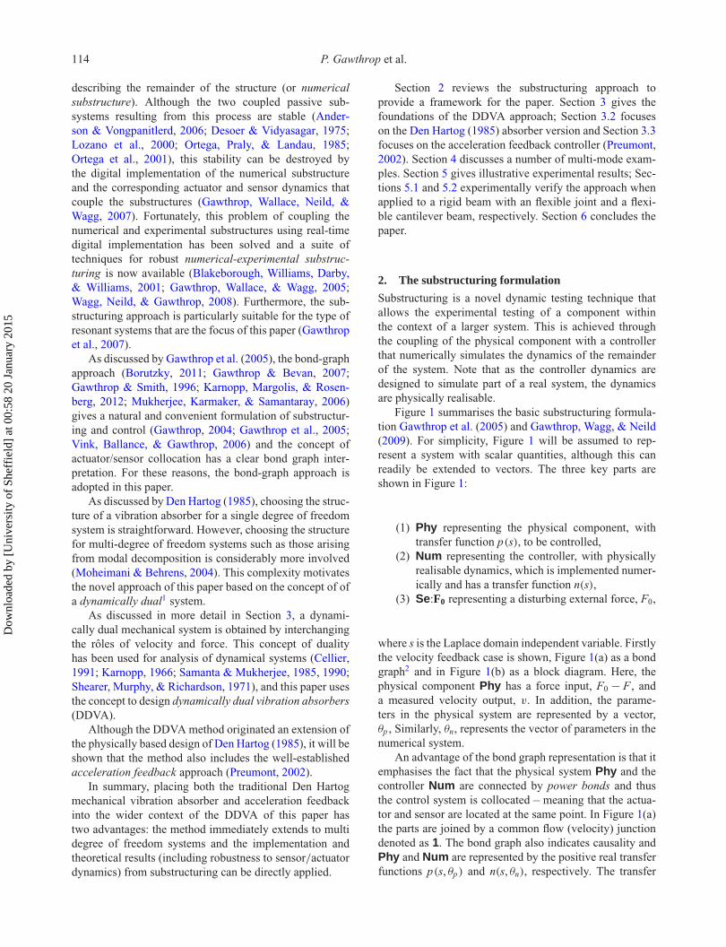
Figure 1 summarises the basic substructuring formula-tion Gawthrop et al. (2005) and Gawthrop, Wagg, & Neild(2009). For simplicity, Figure 1 will be assumed to rep-resent a system with scalar quantities, although this canreadily be extended to vectors. The three key parts areshown in Figure 1:

(1) Phy representing the physical component, withtransfer function p(s), to be controlled,

(2) Num representing the controller, with physicallyrealisable dynamics, which is implemented numer-ically and has a transfer function n(s),

(3) Se:F0 representing a disturbing external force, F0,

where s is the Laplace domain independent variable. Firstlythe velocity feedback case is shown, Figure 1(a) as a bondgraph2 and in Figure 1(b) as a block diagram. Here, thephysical component Phy has a force input, F0 − F , anda measured velocity output, v. In addition, the parame-ters in the physical system are represented by a vector,θp , Similarly, θn, represents the vector of parameters in thenumerical system.

An advantage of the bond graph representation is that itemphasises the fact that the physical system Phy and thecontroller Num are connected by power bonds and thusthe control system is collocated – meaning that the actua-tor and sensor are located at the same point. In Figure 1(a)the parts are joined by a common flow (velocity) junctiondenoted as 1. The bond graph also indicates causality andPhy and Num are represented by the positive real transferfunctions p(s, θp) and n(s, θn), respectively. The transfer

Dow

nloa

ded

by [

Uni

vers

ity o

f Sh

effi

eld]

at 0

0:58

20

Janu

ary

2015

Systems Science & Control Engineering: An Open Access Journal 115

(a) (b)

(c) (d)

Figure 1. The substructuring formulation. The mathematically equivalent formulations (b)–(d) allow for a choice of sensors. (a)Bond graph, (b) block-diagram: velocity formulation, (c) block-diagram: displacement formulation and (d) block-diagram: accelerationformulation.

functions are related by the following relationships:

v = p(s, θp)(F0 − F), (1)

F = n(s, θn)v. (2)

Although it is natural to work in terms of velocityv rather than displacement x, Figure 1(b) can be eas-ily rewritten in terms of displacement as Figure 1(c)where dx/dt = v or in terms of acceleration as Figure 1(d)where a = dv/dt. The choice of formulation (displace-ment, velocity or acceleration) does not change the theo-retical closed-loop stability properties defined by the loop-gain L(s) = n(s, θn)p(s, θp), but allows flexibility in thechoice of sensor and actuator. As well as providing a con-ceptual basis for this paper, the substructuring approachlinks to classical control system concepts useful for stabil-ity and robustness analysis. Details can be found elsewhere(Gawthrop et al., 2007, 2009; Wagg et al., 2008).

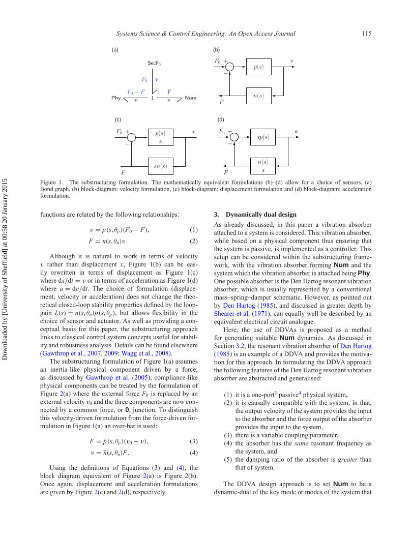
The substructuring formulation of Figure 1(a) assumesan inertia-like physical component driven by a force;as discussed by Gawthrop et al. (2005), compliance-likephysical components can be treated by the formulation ofFigure 2(a) where the external force F0 is replaced by anexternal velocity v0 and the three components are now con-nected by a common force, or 0, junction. To distinguishthis velocity-driven formulation from the force-driven for-mulation in Figure 1(a) an over-bar is used:

F = p̄(s, θp)(v0 − v), (3)

v = n̄(s, θn)F . (4)

Using the definitions of Equations (3) and (4), theblock diagram equivalent of Figure 2(a) is Figure 2(b).Once again, displacement and acceleration formulationsare given by Figure 2(c) and 2(d), respectively.

3. Dynamically dual designAs already discussed, in this paper a vibration absorberattached to a system is considered. This vibration absorber,while based on a physical component thus ensuring thatthe system is passive, is implemented as a controller. Thissetup can be considered within the substructuring frame-work, with the vibration absorber forming Num and thesystem which the vibration absorber is attached being Phy.One possible absorber is the Den Hartog resonant vibrationabsorber, which is usually represented by a conventionalmass–spring–damper schematic. However, as pointed outby Den Hartog (1985), and discussed in greater depth byShearer et al. (1971), can equally well be described by anequivalent electrical circuit analogue.

Here, the use of DDVAs is proposed as a methodfor generating suitable Num dynamics. As discussed inSection 3.2, the resonant vibration absorber of Den Hartog(1985) is an example of a DDVA and provides the motiva-tion for this approach. In formulating the DDVA approachthe following features of the Den Hartog resonant vibrationabsorber are abstracted and generalised:

(1) it is a one-port3 passive4 physical system,(2) it is causally compatible with the system, in that,

the output velocity of the system provides the inputto the absorber and the force output of the absorberprovides the input to the system,

(3) there is a variable coupling parameter,(4) the absorber has the same resonant frequency as

the system, and(5) the damping ratio of the absorber is greater than

that of system.

The DDVA design approach is to set Num to be adynamic-dual of the key mode or modes of the system that

Dow

nloa

ded

by [

Uni

vers

ity o

f Sh

effi

eld]

at 0

0:58

20

Janu

ary

2015

116 P. Gawthrop et al.

(a) (b)

(c) (e)

Figure 2. The velocity-driven substructuring formulation. (a) Bond graph, (b) block-diagram: velocity formulation, (c) block-diagram:displacement formulation and (d) block-diagram: acceleration formulation.

the absorber is attached to (which is contained in Phy).The method of obtaining a dynamic dual is now discussed.This is followed by discussions of two common absorberstrategies which are DDVA; the Den Hartog absorber andthe acceleration feedback method proposed by Preumont(2002).

3.1. A dynamic-dualA dynamic-dual of a system is obtained by interchangingthe rôles of velocity and force, is defined in Shearer et al.(1971). An extended version of this concept, the scaleddual is used here and, in the context of mechanical systemsis defined as follows:

(1) Each force Fi, and each velocity vi, in the originalsystem has a scaled dual vD

i , and FDi in the dual

system given by:

vDi = 1

gFi, (5)

FDi = gvi, (6)

where g is the scaling factor and g = 1 correspondsto the unscaled dual.

(2) Each mass component with mass mi is replaced inthe dual system with a spring component of stiff-ness Ki, each spring component with stiffness kiis replaced in the dual system with a mass com-ponent of mass Mi, and each damper componentwith damping coefficient ri is replaced in the dualsystem with a damper component with dampingcoefficient Ri where:

Ki = g2

mi, (7)

Mi = g2

ki, (8)

Ri = g2

ri. (9)

(3) Common force connections become commonvelocity connections and common velocity con-nections become common force connections in thedual system.

(4) If the system transfer function h(s) has force F asinput and velocity v as output, then the dual trans-fer function H(s) has velocity vD as input and forceFD as output and is given by:

FD = gv, (10)

vD = 1g

F , (11)

H(s) = FD

vD = gv

(1/g)F= g2h(s). (12)

Equations (10) and (11) are power conserving in the sensethat

FDvD = Fv. (13)

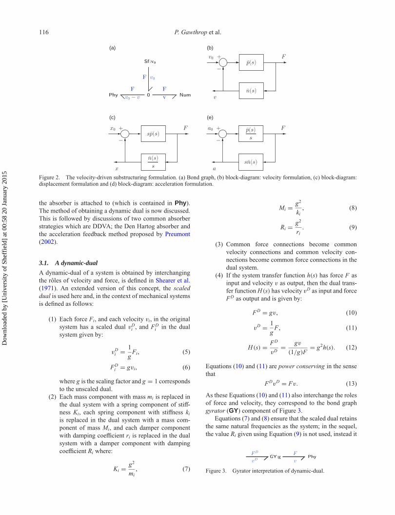
As these Equations (10) and (11) also interchange the rolesof force and velocity, they correspond to the bond graphgyrator (GY) component of Figure 3.

Equations (7) and (8) ensure that the scaled dual retainsthe same natural frequencies as the system; in the sequel,the value Ri given using Equation (9) is not used, instead it

Figure 3. Gyrator interpretation of dynamic-dual.

Dow

nloa

ded

by [

Uni

vers

ity o

f Sh

effi

eld]

at 0

0:58

20

Janu

ary

2015

Systems Science & Control Engineering: An Open Access Journal 117

is replaced by the user-selected value R′i. This allows the

damping of the modified scaled dual system, which formsthe controller implemented in Num, to be adjusted.

Although not essential to the approach of this paper, thebond graph formulation provides a clear exposition of thenotion of a scaled dual. In particular, the scaled dual systemcan be described in two different but equivalent ways as:

(1) the bond graph dual where the component moduliare given by Equations (7)–(9) or

(2) following Equation (13), the system obtained byappending a gyrator of modulus g to the sys-tem Phy port as in Figure 3. This point is alsodiscussed by Gawthrop et al. (2010).

3.2. Den Hartog absorberIn his classical text book (Den Hartog, 1985, Section 3.3),Den Hartog considers the design of a damped vibrationabsorber for an undamped mass–spring system which issubject to a force disturbance. The specifications

(1) ‘the main mass is 20 times greater than the dampermass’,

(2) ‘the frequency of the damper is equal to the fre-quency of the main system’,

(3) The damping ratio of the damper is ζ = 0.1.

were considered.In the terminology used in this paper, the physical sys-

tem requiring vibration suppression (Phy) is the undampedmass–spring oscillator. In Den Hartog (1985) the vibra-tion absorber was considered to be a physical mechan-ical device but here it is considered to be a controller(with sensor and actuator) with the same dynamics as theabsorber and forms Num. The disturbance force acts onthe undamped mass–spring oscillator Phy, as does a forcedue to the presence of the absorber Num, therefore thesystem can be represented by the block diagram given inFigure 1(b).

Figure 4(b) and 4(a) gives the schematic diagram ofthe damped vibration absorber Num and the undampedoscillator Phy, respectively. A damper with r = ∞ isincluded in the subsystem Phy of Figure 4(a) to allowfor the corresponding component in the subsystem Num.Using standard manipulations, the transfer function of thephysical system, Phy, of Figure 4(a) is:

p(s, θp) = s(ms + r)mrs2 + kms + kr

. (14)

Letting r → ∞ gives:

p(s, θp) = sms2 + k

. (15)

Similarly, from Figure 4(b), the transfer function for Num,which represents the Den Hartog absorber, is

n(s, θn) = Ms(Rs + K)

Ms2 + Rs + K. (16)

It can be shown that this absorber is a scaled dynamic-dual of the system, Phy, it is applied to. Considering thesystem Phy, given in Equation (14), and applying the dualtransforms, given in Equations (7)–(9), the parameters m,k and r can be rewritten in terms of M ,K and D to give:

p(s, θp)

= s((g2/k)s + (g2/R))

(g2/k)(g2/R)s2 + (g2/M )(g2/K)s + (g2/M )(g2/R)

=(

1g2

)Ms(Rs + K)

Ms2 + Rs + Kr. (17)

Applying the scaling given in Equation (12), the scaleddual of Phy is

P(s, �p) = g2p(s, θp) = Ms(Rs + K)

Ms2 + Rs + Kr. (18)

Thus, by comparing this to Equation (16), it can be seenthat the Den Hartog absorber in Num corresponds to thescaled dual of Phy:

n(s, θn) = P(s, �p). (19)

The first part of the Den Hartog specifications isachieved by setting:

M = αm where α = 120

. (20)

The second part of the specification is achieved by setting

KM

= km

. (21)

Equations (20) and (21) imply that

K = αk. (22)

Moreover, using Equations (7) and (22), the scaling gain gis given by

g2 = Km = αmk. (23)

Dow

nloa

ded

by [

Uni

vers

ity o

f Sh

effi

eld]

at 0

0:58

20

Janu

ary

2015

118 P. Gawthrop et al.

100

10

1

0.1

0.1 1 10w rad/sec

Yc(

jw)

Yc(

t)

0.01

1

0.5

0

–0.5

–10 20 40 60 80 100

t(sec)

(a) (b)

(c) (d)

Figure 4. Den Hartog absorber. The physical system (a) and its vibration absorber (and dynamic-dual) (b) are first-order mass–spring—damper systems. (c) The closed-loop frequency response (black line) has a lower resonant peak than the open-loop response (grey line).(d) The closed-loop impulse response (black line) exhibits more damping than the open-loop impulse response (grey line). (a) Phy: thephysical system, (b) Num: the dual physical system, (c) frequency response H(j ω) and (d) impulse response h(t).

Finally, the third part of the specification is achieved byreplacing the damping coefficient R of n(s, θn) by

R′ = 2ζ√

MK . (24)

To illustrate the properties of this particular vibrationabsorber, the unit system with m = k = 1 was used. Usingthe specification described above, this gives the numericalsystem parameters M = K = 0.05 and R′ = 0.01, and sothe DDVA is given by:

n(s, θ ′n) = Ms(R′s + K)

Ms2 + R′s + K= 0.01s2 + 0.05s

s2 + 0.2s + 1. (25)

The corresponding closed-loop frequency responseappears in Figure 4(c); this shows the ‘split peak’ phe-nomenon described by Den Hartog (1985). The cor-responding closed-loop impulse response appears inFigure 4(d); this decays exponentially over the time scalesdetermined by the specified damping ratio.

3.3. Acceleration feedbackThe acceleration feedback method has been proposed byPreumont (2002). This section rederives the algorithmfrom the DDVA point of view. In particular, the undampedphysical system of Figure 4(a) (with 1/r = 0) can equallywell be represented in Figure 5(a) with r = 0. This sys-tem has a different modified dual and thus gives a differentform of control; this turns out to be a form of accelerationfeedback.

As with the last example the vibration absorber is act-ing on an undamped mass–spring oscillator. The undampedoscillator forms Phy as shown in Figure 5(a). Note that adamper with r = 0 is included to allow a dynamic-dual tobe formulated. Using standard manipulations, the transferfunction of the physical system Phy of Figure 5(a) is

p(s, θp) = sms2 + rs + k

. (26)

Dow

nloa

ded

by [

Uni

vers

ity o

f Sh

effi

eld]

at 0

0:58

20

Janu

ary

2015

Systems Science & Control Engineering: An Open Access Journal 119

0.01

0.1

1

10

100

Yc(

t)0.5

–0.5

–1

(d)(c)

(b)(a)

0.1 1 10w rad/sec

0 20 40 60 80 100t(sec)

Yc(

jw)

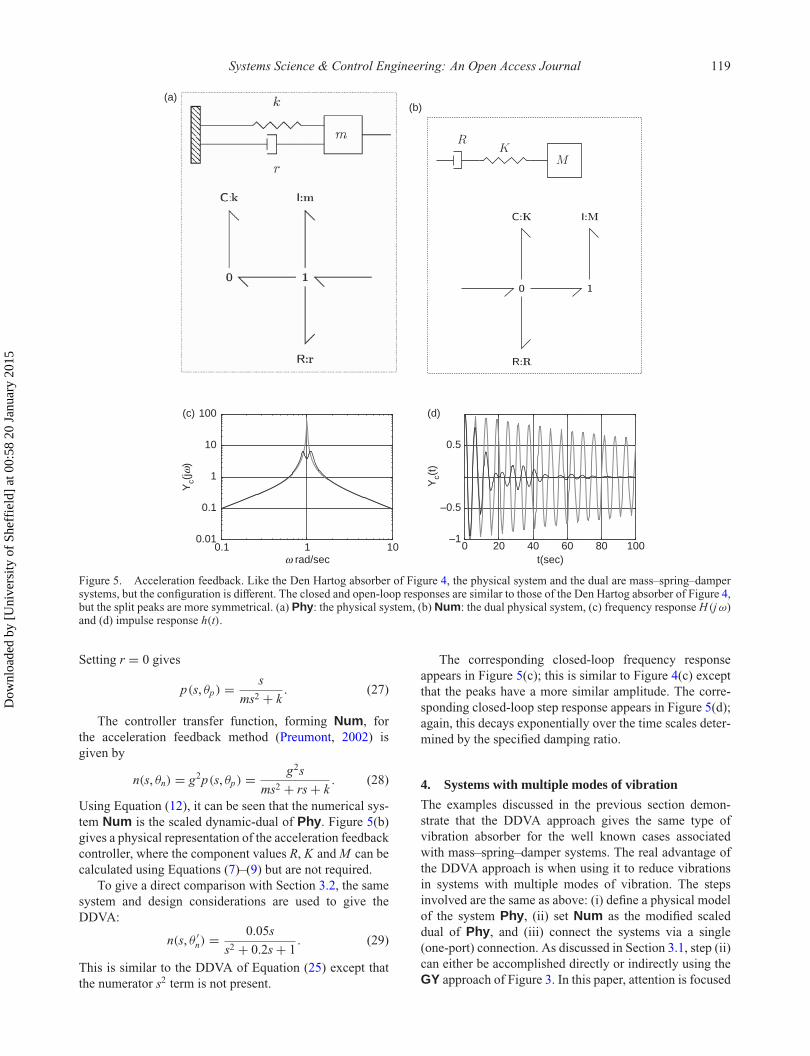
Figure 5. Acceleration feedback. Like the Den Hartog absorber of Figure 4, the physical system and the dual are mass–spring–dampersystems, but the configuration is different. The closed and open-loop responses are similar to those of the Den Hartog absorber of Figure 4,but the split peaks are more symmetrical. (a) Phy: the physical system, (b) Num: the dual physical system, (c) frequency response H(j ω)and (d) impulse response h(t).

Setting r = 0 gives

p(s, θp) = sms2 + k

. (27)

The controller transfer function, forming Num, forthe acceleration feedback method (Preumont, 2002) isgiven by

n(s, θn) = g2p(s, θp) = g2sms2 + rs + k

. (28)

Using Equation (12), it can be seen that the numerical sys-tem Num is the scaled dynamic-dual of Phy. Figure 5(b)gives a physical representation of the acceleration feedbackcontroller, where the component values R, K and M can becalculated using Equations (7)–(9) but are not required.

To give a direct comparison with Section 3.2, the samesystem and design considerations are used to give theDDVA:

n(s, θ ′n) = 0.05s

s2 + 0.2s + 1. (29)

This is similar to the DDVA of Equation (25) except thatthe numerator s2 term is not present.

The corresponding closed-loop frequency responseappears in Figure 5(c); this is similar to Figure 4(c) exceptthat the peaks have a more similar amplitude. The corre-sponding closed-loop step response appears in Figure 5(d);again, this decays exponentially over the time scales deter-mined by the specified damping ratio.

4. Systems with multiple modes of vibrationThe examples discussed in the previous section demon-strate that the DDVA approach gives the same type ofvibration absorber for the well known cases associatedwith mass–spring–damper systems. The real advantage ofthe DDVA approach is when using it to reduce vibrationsin systems with multiple modes of vibration. The stepsinvolved are the same as above: (i) define a physical modelof the system Phy, (ii) set Num as the modified scaleddual of Phy, and (iii) connect the systems via a single(one-port) connection. As discussed in Section 3.1, step (ii)can either be accomplished directly or indirectly using theGY approach of Figure 3. In this paper, attention is focused

Dow

nloa

ded

by [

Uni

vers

ity o

f Sh

effi

eld]

at 0

0:58

20

Janu

ary

2015

120 P. Gawthrop et al.

Table 1. Modal system: resonant fre-quencies.

n ωn (rad/s)

1 1.02 2.0

on linear models thus giving rise to transfer-function rep-resentations.

Two examples are considered here. The first is a twodegree-of-freedom lumped mass system which is shownschematically in Figure 6(a) and 6(b). Figure 6(a) and 6(b)are similar to Figure 5(a) and 5(b) except that there are twocoupled mass–spring damper systems involved. Thus Phycan be regarded as the modal decomposition of a 2DOFsystem and Num the corresponding vibration absorber.For the purposes of illustration, each subsystem of Numhas the same parameters as in the example of Figure 5 ofSection 3.3 (Table 1).

Figure 6(c) shows the open (without the vibrationabsorber) and closed-loop (with the vibration absorber)frequency response magnitudes. The magnitude of theclosed-loop response (black line) is clearly smaller thanthe corresponding open-loop response (grey line) at thetwo resonant frequencies. Figure 6(d) shows the equivalentimpulse response; as predicted by the frequency responses,the closed-loop impulse response decays more rapidly thanthe equivalent open-loop response.

As a second example, a uniform Euler-Bernoulli5 can-tilever beam (with one end fixed and the other free)modelled using a 10 element, finite-element bond graphmodel (Karnopp, Margolis, & Rosenberg, 2000; Margo-lis, 1985) is considered. Such beam models are undamped;but the DDVA approach needs to include damping inNum. For the purposes of this example, Rayleigh damp-ing is assumed; in particular, each compliant element in thelumped model has an associated damping term representedby a damper connected across the ends of the compliantelements.

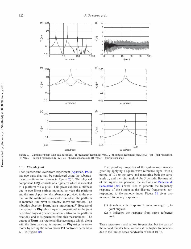
Following Balas (1978, Section V) who considers a‘unit beam’, the cantilever beam is normalised to have unitmass per unit length and unit compliance per unit length.Phy is assumed to have a small (but non-zero) dampingof 10−6 per unit length. The 10 modal frequencies appearin Table 2. For the purposes of illustration, the vibrationabsorber was applied to the beam using a collocated pointForce/Velocity actuator/sensor halfway along the beam. Asdiscussed in the sequel, this point corresponds to a nodalpoint of the third-resonance and thus this mode cannot becontrolled with this choice. The choice of actuator/sensorlocation is an interesting topic not considered in this paper.

Two versions of DDVA were used. The first DDVAwas obtained by considering the complete dynamic-dualof Phy. The scaled dual Num was obtained using the GYapproach of Figure 3. A feature of this approach is that

Table 2. Cantilever beam model modal fre-quencies.

n ωn (rad/s)

1 2.9192 18.283 50.374 95.595 150.46 210.07 269.18 322.09 363.910 390.8

Note: Not all frequencies appear in Figures 7and 8 due to coincident zeros.

there are only two control parameters. These were cho-sen as the gyrator gain g2 = 0.05 and the damping of thecantilever beam model in Num as 2 per unit length.

Figure 7(a) shows the open (without the vibrationabsorber) and closed-loop (with the vibration absorber)frequency response magnitudes. This figure has beenexpanded to show the frequency responses close to thefirst–fourth resonances in Figure 7(c)–7(f), respectively.Near the first two resonances (Figure 7(c) and 7(d)), themagnitude of the closed-loop response (black line) isclearly smaller than the corresponding open-loop response(grey line) at the two resonant frequencies. The third reso-nance corresponds to a node at the sensor/actuator and thefourth is well damped anyway. Thus this controller designnaturally applies control authority at the important reso-nances. Figure 7(b) shows the equivalent impulse response;as predicted by the frequency responses, the closed-loopimpulse response decays more rapidly than the equivalentopen-loop response. As noted above, the third resonanceis not controlled using this approach. However, it could becontrolled either by moving the sensor/actuator away fromthe node or by having a second sensor/actuator away fromthe node.

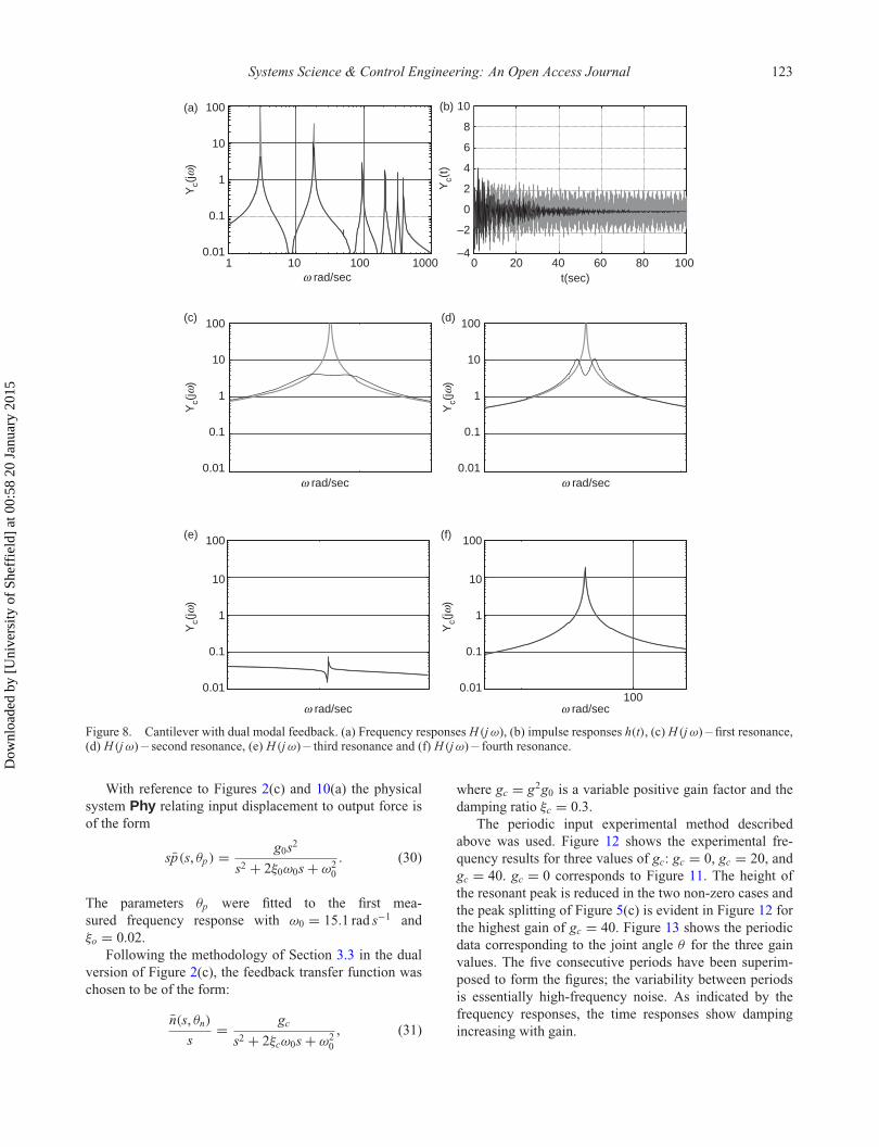
The second approach is to use the scaled dynamic-dualof a two mode modal model (as in Figure 6(b)), capturingthe dynamics of the first two modes of the cantilever. Thisis then connected to the same cantilever beam. The parame-ters of Num are the same as in the example of Figure 6 andthose of Phy the same as those of the example of Figure 7.

Figure 8(a) shows the open (without the vibrationabsorber) and closed-loop (with the vibration absorber)frequency response magnitudes. This figure has beenexpanded to show the frequency responses close to thefirst–fourth resonances in Figure 8(c)–8(f), respectively.Near the first two resonances (Figure 8(c) and 8(d)), themagnitude of the closed-loop response (black line) isclearly smaller than the corresponding open-loop response(grey line) at the two resonant frequencies; these Fig-ures are not the same as Figure 7(c) and 7(d) because

Dow

nloa

ded

by [

Uni

vers

ity o

f Sh

effi

eld]

at 0

0:58

20

Janu

ary

2015

Systems Science & Control Engineering: An Open Access Journal 121

100

10

1

0.1

0.1 1 10w rad/sec

Yc(

jw)

0.01

(c)

Yc(

t)

2

1.5

0.5

1

0

–0.5

–10 20 40 60 80 100

t(sec)

(d)

(a) (b)

Figure 6. Modal system. Both the physical system and its dual are coupled mass–spring–damper systems and are thus fourth-order. (c)The closed-loop frequency response (black line) has both resonant peaks lower than the open-loop response (grey line). (d) Again, theclosed-loop impulse response (black line) exhibits more damping than the open-loop impulse response (grey line). (a) Phy: the physicalsystem, (b) Num: the dual physical system, (c) frequency response H(j ω) and (d) impulse response h(t).

the controller is different; but the effect is similar. Thethird and fourth resonances are explicitly not controlledwith this method; but, in this case, the effect is the sameas that of the controller of the example of Figure 7.In particular Figure 8(b) shows that the closed-loopimpulse response decays more rapidly than the equiva-lent open-loop response in a similar fashion to that ofFigure 7(b). In this particular example, the performance ofthe two controllers is quite similar.

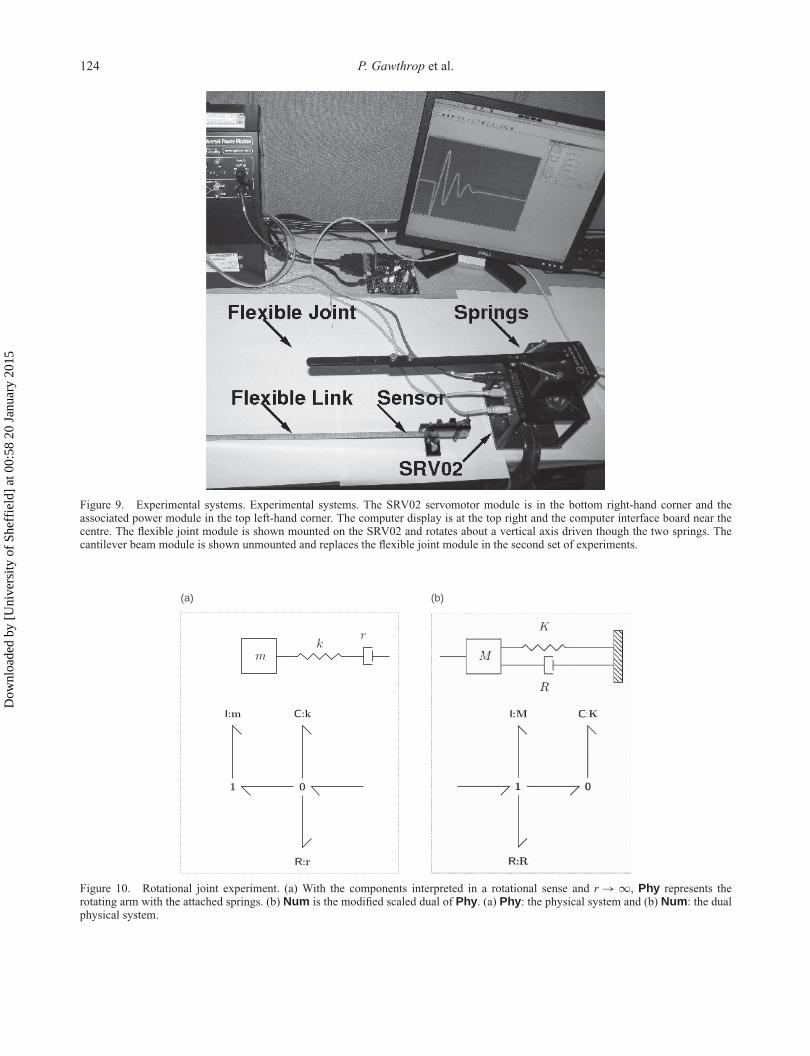
5. Experimental resultsAs indicated in Figure 9, the experiments were based on theQuanser (Apkarian, 1995) SRV02 rotational servo-motorand associated UPM-15-03-240 power and instrumentation

module. The SRV02 was firmly clamped to a rigidbench and interfaced to a Intel CoreTM 2 Duo Proces-sor (2.66 GHz) based computer via a National InstrumentsPCI-8024E analogue-digital conversion card and cable andthe corresponding Quanser interface board.

In the experiment described here, the computer used thereal-time Linux operating system RTAI together with thecontrol-orientated software RTAI-Lab (Bucher & Balemi,2006) running at a sampling frequency of 500 Hz. Usingthis software, the SRV02 rotational servo motor, rota-tional position sensor and associated power supply werecontrolled to give high-gain position control using a pro-portional and derivative (PD) controller. The servo anglewas measured using a potentiometer and scaled within thecomputer to measure angular position in radians.

Dow

nloa

ded

by [

Uni

vers

ity o

f Sh

effi

eld]

at 0

0:58

20

Janu

ary

2015

122 P. Gawthrop et al.

0.01

0.1

1

10

100

1 10 100 1000w rad/sec

Yc(

jw)

–4

–2

0

2

4

6

8

10

0 20 40 60 80 100t(sec)

Yc(

t)

0.01

0.1

1

10

100

w rad/sec

Yc(

jw)

0.01

0.1

1

10

100

w rad/sec

Yc(

jw)

0.01

0.1

1

10

100

Yc(

jw)

w rad/sec

0.01

0.1

1

10

100

100

Yc(

jw)

w rad/sec

(c) (d)

(e) (f)

(a) (b)

Figure 7. Cantilever beam with dual feedback. (a) Frequency responses H(j ω), (b) impulse responses h(t), (c) H (j ω) – first resonance,(d) H(j ω) – second resonance, (e) H(j ω) – third resonance and (f) H(j ω) – fourth resonance.

5.1. Flexible jointThe Quanser cantilever beam experiment (Apkarian, 1995)has two parts that may be considered using the substruc-turing configuration shown in Figure 2(c). The physicalcomponent, Phy, consists of a rigid arm which is mountedto a platform via a pivot. This pivot exhibits a stiffnessdue to two linear springs mounted between the platformand the arm. A position disturbance is provided to the sys-tem via the rotational servo motor on which the platformis mounted (the pivot is directly above the motor). Thevibration absorber, Num, has a torque input F . Because ofthe springs in Phy, this torque is proportional to the jointdeflection angle θ (the arm rotation relative to the platformrotation), and so is generated from this measurement. Theoutput of Num is a rotational displacement x which, alongwith the disturbance x0, is imposed on Phy using the servomotor by setting the servo motor PD controller demand tox0 − x (Figure 10).

The open-loop properties of the system were investi-gated by applying a square-wave reference signal with aperiod of 10 s to the servo and measuring both the servoangle xa and the joint angle θ for 5 periods. Because allof the signals are periodic, the methods of Pintelon &Schoukens (2001) were used to generate the frequencyresponse of the system at the discrete frequencies cor-responding to the periodic input. Figure 11 gives twomeasured frequency responses:

(1) + indicates the response from servo angle xa tojoint angle θ .

(2) ◦ indicates the response from servo referenceto θ .

These responses match at low frequencies, but the gain ofthe second transfer function falls at the higher frequenciesdue to the limited servo bandwidth of about 10 Hz.

Dow

nloa

ded

by [

Uni

vers

ity o

f Sh

effi

eld]

at 0

0:58

20

Janu

ary

2015

Systems Science & Control Engineering: An Open Access Journal 123

100

0.01

0.1

1

10

100

Yc(

jw)

(a)

1 10 100 1000w rad/sec

–4

–2

0

2

4

6

8

10

0 20 40 60 80 100t(sec)

Yc(

t)

(b)

0.01

0.1

1

10

100

w rad/sec w rad/sec

Yc(

jw)

(c)

0.01

0.1

1

10

100

Yc(

jw)

(e)

0.01

0.1

1

10

100

Yc(

jw)

(f)

0.01

0.1

1

10

100

Yc(

jw)

(d)

w rad/sec w rad/sec

Figure 8. Cantilever with dual modal feedback. (a) Frequency responses H(j ω), (b) impulse responses h(t), (c) H (j ω) – first resonance,(d) H(j ω) – second resonance, (e) H(j ω) – third resonance and (f) H(j ω) – fourth resonance.

With reference to Figures 2(c) and 10(a) the physicalsystem Phy relating input displacement to output force isof the form

sp̄(s, θp) = g0s2

s2 + 2ξ0ω0s + ω20

. (30)

The parameters θp were fitted to the first mea-sured frequency response with ω0 = 15.1 rad s−1 andξo = 0.02.

Following the methodology of Section 3.3 in the dualversion of Figure 2(c), the feedback transfer function waschosen to be of the form:

n̄(s, θn)

s= gc

s2 + 2ξcω0s + ω20

, (31)

where gc = g2g0 is a variable positive gain factor and thedamping ratio ξc = 0.3.

The periodic input experimental method describedabove was used. Figure 12 shows the experimental fre-quency results for three values of gc: gc = 0, gc = 20, andgc = 40. gc = 0 corresponds to Figure 11. The height ofthe resonant peak is reduced in the two non-zero cases andthe peak splitting of Figure 5(c) is evident in Figure 12 forthe highest gain of gc = 40. Figure 13 shows the periodicdata corresponding to the joint angle θ for the three gainvalues. The five consecutive periods have been superim-posed to form the figures; the variability between periodsis essentially high-frequency noise. As indicated by thefrequency responses, the time responses show dampingincreasing with gain.

Dow

nloa

ded

by [

Uni

vers

ity o

f Sh

effi

eld]

at 0

0:58

20

Janu

ary

2015

124 P. Gawthrop et al.

Figure 9. Experimental systems. Experimental systems. The SRV02 servomotor module is in the bottom right-hand corner and theassociated power module in the top left-hand corner. The computer display is at the top right and the computer interface board near thecentre. The flexible joint module is shown mounted on the SRV02 and rotates about a vertical axis driven though the two springs. Thecantilever beam module is shown unmounted and replaces the flexible joint module in the second set of experiments.

(a) (b)

Figure 10. Rotational joint experiment. (a) With the components interpreted in a rotational sense and r → ∞, Phy represents therotating arm with the attached springs. (b) Num is the modified scaled dual of Phy. (a) Phy: the physical system and (b) Num: the dualphysical system.

Dow

nloa

ded

by [

Uni

vers

ity o

f Sh

effi

eld]

at 0

0:58

20

Janu

ary

2015

Systems Science & Control Engineering: An Open Access Journal 125

Figure 11. Flexible joint: open-loop frequency responses. Flex-ible joint: open-loop frequency responses. + indicates theresponse from servo angle x to joint angle θ ; ◦ indicates theresponse from servo reference to θ . The solid line is the fittedfrequency response.

Figure 12. Flexible joint: closed-loop frequency responses.

5.2. Cantilever beamThe flexible joint module was replaced by the cantileverbeam module in Figure 9. A strain gauge measures the cur-vature at the root of the cantilever beam. In the same wayas the joint potentiometer of Section 5.1 provided a voltageproportional to torque F , the strain gauge sensor provides avoltage proportional to torque F . The open-loop responsewas measured using the same methods. Two resonancesand one anti-resonance appear in the measured frequencyresponse and similarly to Section 5.1, this was fitted by atransfer function of the form:

sp̄(s, θp) = g0

[κ1s2

s2 + 2ξ1ω1s + ω21

+ κ2s2

s2 + 2ξ2ω2s + ω22

]

(32)

with ω1 = 23.25 rad s−1,ω2 = 159.00 rad s−1, ξ1 = ξ2 =0.04, κ1 = 0.36 and κ2 = 1 − κ1 = 0.64. Because of the10 Hz servo bandwidth, the discrepancy between measuredand fitted transfer function is large above 10 Hz.

Following the methodology of Section 4 a two-modetransfer function corresponding to Equation (33) was

(a)

(b)

(c)

Figure 13. Flexible joint: time responses. (a) gc = 0, (b)gc = 20 and (c) gc = 40.

Figure 14. Cantilever beam: open-loop frequency responses.Cantilever beam: open-loop frequency responses. + indicates theresponse from servo angle x to joint angle θ . The firm line is thefitted frequency response.

Dow

nloa

ded

by [

Uni

vers

ity o

f Sh

effi

eld]

at 0

0:58

20

Janu

ary

2015

126 P. Gawthrop et al.

Figure 15. Cantilever beam: closed-loop frequency responsesfor the cases where gc = 0, 50 and 100.

(a)

(b)

(c)

Figure 16. Cantilever beam: time responses. (a) gc = 0, (b)gc = 50 and (c) gc = 100.

chosen as:

n̄(s, θn)

s= gc

[κ1s2

s2 + 2ξcω1s + ω21

+ κ2s2

s2 + 2ξcω2s + ω22

]

(33)

with ξc = 0.3.

The periodic input experimental method describedabove was used. Figure 15 shows the experimental fre-quency results for three values of gc: gc = 0, gc = 50, andgc = 100. gc = 0 corresponds to Figure 14. The heightof the first resonant peak is reduced in the two non-zerocases and the peak splitting of Figure 8(a) is evident inFigure 15 for both cases. The second resonance is largelyunaffected; we attribute this to the limited actuator band-width. Figure 16 shows the periodic data correspondingto the measured strain voltage σ for the three gain val-ues. As with Figure 13, five consecutive periods have beensuperimposed to form the figures showing that the vari-ability between periods is essentially high-frequency noise.Again, as indicated by the frequency responses, the timeresponses show damping increasing with gain.

6. ConclusionThe DDVA approach has been shown to provide a novelmethod to design vibration absorbers in the physicaldomain. In particular, the method is a natural generalisationof not only the classical single-degree of freedom vibra-tion absorber of Den Hartog (1985, Section 3.3) but alsoof acceleration feedback (Preumont, 2002). Placing thesetwo well-known design methods into the wider context ofthe DDVA of this paper has the following advantages: themethods immediately extend to multi degree of freedomsystems and the implementation and theoretical results(including robustness to sensor/actuator dynamics) fromsubstructuring can be directly applied.

The DDVA approach has been illustrated using numer-ical simulations of single mode and multi-mode systemsand verified using two experimental systems: a rigid beamwith an flexible joint and a flexible cantilever beam. Futurework will apply the results to more complex dynami-cal systems including those with multiple sensor-actuatorpairs.

The location of the sensor-actuator pairs has not beenconsidered in this paper even though it certainly affectscontrollability and observability issues (Balas, 1978).Future work in this area will extend bond graph approaches(for example those of Marquis-Favre & Jardin (2011) andGawthrop & Rizwi (2011)) to sensor/actuator placementin this context.

In principle, the method is equally applicable to thecontrol nonlinear vibrations where dynamical dual of thenonlinear physical system provides the basis for a nonlin-ear controller. This is also an area for future work.

AcknowledgementsPeter Gawthrop was a Visiting Research Fellow at The Universityof Bristol when this work was accomplished; he is now supportedby a Professorial Fellowship at the University of Melbourne.

Dow

nloa

ded

by [

Uni

vers

ity o

f Sh

effi

eld]

at 0

0:58

20

Janu

ary

2015

Systems Science & Control Engineering: An Open Access Journal 127

Disclosure statementNo potential conflict of interest was reported by the authors.

FundingSimon Neild is supported by EPSRC fellowship EP/K005375/1.David Wagg is supported by EPSRC [grant EP/K003836/2].

Notes

1. As the word ‘dual’ has many meanings, the term dynamicallydual is used for the specific meaning of this paper.

2. The bond directions have been changed for this paper to cor-respond to the usual sign convention for feedback controlblock diagrams.

3. ‘One-port’ refers to the single energy port associated withforce and velocity

4. In the sense that it consumes but does not produce energy.5. Other models such as the Timoshenko model, as well as

non-uniform beams, could similarly be handled using thisapproach

ReferencesAli, S. F., & Padhi, R. (2009). Active vibration suppression of

non-linear beams using optimal dynamic inversion. Journalof Systems and Control Engineering, 223(5), 657–672.

Anderson, B. D. O., & Vongpanitlerd, S. (2006). Network analy-sis and synthesis a modern systems theory approach. Dover.First published 1973 by Prentice-Hall.

Apkarian, J. (1995). A comprehensive and modular laboratoryfor control systems design and implementation. Markham,Ontario: Quanser Consulting.

Balas, M. J. (1978). Feedback control of flexible systems. IEEETransactions on Automatic Control, 23(4), 673–679.

Blakeborough, A., Williams, M. S., Darby, A. P., & Williams, D.M. (2001). The development of real-time substructure test-ing. Philosophical Transactions of the Royal Society Part A,359, 1869–1891.

Borutzky, W. (2011). Bond graph modelling of engineeringsystems: Theory, applications and software support. NewYork, NY: Springer.

Bucher, R., & Balemi, S. (2006). Rapid controller prototyp-ing with matlab/simulink and linux. Control EngineeringPractice, 14(2), 185–192.

Cellier, F. E. (1991). Continuous system modelling. Berlin:Springer-Verlag.

Den Hartog, J. P. (1985). Mechanical vibrations. Dover. Reprintof 4th ed. Published by McGraw-Hill 1956.

Desoer, C. A., & Vidyasagar, M. (1975). Feedback systems:Input-output properties. London: Academic Press.

Fleming, A. J., & Moheimani, S. O. R. (2005). Control ori-entated synthesis of high-performance piezoelectric shuntimpedances for structural vibration control. IEEE Transac-tions on Control Systems Technology, 13(1), 98–112.

Gawthrop, P. J. (1995). Physical model-based control: A bondgraph approach. Journal of the Franklin Institute, 332B(3),285–305.

Gawthrop, P. J. (2004). Bond graph based control using vir-tual actuators. Proceedings of the Institution of MechanicalEngineers Pt. I: Journal of Systems and Control Engineer-ing, 218(4), 251–268.

Gawthrop, P. J., & Bevan, G. P. (2007). Bond-graph modeling:A tutorial introduction for control engineers. IEEE ControlSystems Magazine, 27(2), 24–45.

Gawthrop, P. J., & Rizwi, F. (2011). Coaxially coupled invertedpendula: Bond graph-based modelling, design and control.In W. Borutzky (Ed.), Bond graph modelling of engineeringsystems (pp. 179–194). New York, NY: Springer.

Gawthrop, P. J., & Smith, L. P. S. (1996). Metamodelling: Bondgraphs and dynamic systems. Hemel Hempstead: PrenticeHall.

Gawthrop, P. J., Bhikkaji, B., & Moheimani, S. O. R. (2010).Physical-model-based control of a piezoelectric tube fornano-scale positioning applications. Mechatronics, 20(1),74–84. Available online 13 October 2009.

Gawthrop, P. J., Wagg, D. J., & Neild, S. A. (2009). Bond graphbased control and substructuring. Simulation ModellingPractice and Theory, 17(1), 211–227. Available online 19November 2007.

Gawthrop, P. J., Wallace, M. I., Neild, S. A., & Wagg,D. J. (2007). Robust real-time substructuring tech-niques for under-damped systems. Structural Control andHealth Monitoring, 14(4), 591–608. Published on-line:19 May 2006.

Gawthrop, P. J., Wallace, M. I., & Wagg, D. J. (2005).Bond-graph based substructuring of dynamical systems.Earthquake Engineering & Structural Dynamics, 34(6),687–703.

Hagood, N. W., & von Flotow, A. (1991). Damping of structuralvibrations with piezoelectric materials and passive electricalnetworks. Journal of Sound and Vibration, 146(2), 243–268.

Hogan, N. (1985). Impedance control: An approach to manipu-lation. part I – theory. ASME Journal of Dynamic Systems,Measurement and Control, 107, 1–7.

Høgsberg, J. R., & Krenk, S. (2006). Linear control strategiesfor damping of flexible structures. Journal of Sound andVibration, 293(1–2), 59–77.

Hong, J. H., & Bernstein, D. S. (1998). Bode integral constraints,colocation, and spillover in active noise and vibrationcontrol. IEEE Transactions on Control Systems Technology,6(1), 111–120.

Karnopp, D. (1966). Coupled vibratory-system analysis, using thedual formulation. The Journal of the Acoustical Society ofAmerica, 40(2), 380–384.

Karnopp, D., Margolis, D. L., & Rosenberg, R. C. (2000). Sys-tem dynamics: Modeling and simulation of mechatronicsystems (3rd ed.). New York, NY: Horizon Publishers andDistributors Inc.

Karnopp, D. C., Margolis, D. L., & Rosenberg, R. C. (2012).System dynamics: Modeling, simulation, and control ofmechatronic systems (5th ed.). John Wiley & Sons.

Krenk, S., & Hogsberg, J. (2009). Optimal resonant control offlexible structures. Journal of Sound and Vibration. 323(3–5), 530–554.

Lozano, R., Brogliato, B., Egelund, O., & Maschke, B. (2000).Dissipative systems: Analysis and control. New York, NY:Springer.

Margolis, D. L. (1985). A survey of bond graph modelling forinteracting lumped and distributed systems. Journal of theFranklin Institute, 319, 125–135.

Marquis-Favre, W., & Jardin, A. (2011). Bond graphs and inversemodeling for mechatronic system design. In W. Borutzky(Ed.), Bond graph modelling of engineering systems (pp.195–226). New York, NY: Springer.

Moheimani, S. O. R, & Behrens, S. (2004). Multimode piezo-electric shunt damping with a highly resonant impedance.IEEE Transactions on Control Systems Technology, 12(3),484–491.

Dow

nloa

ded

by [

Uni

vers

ity o

f Sh

effi

eld]

at 0

0:58

20

Janu

ary

2015

128 P. Gawthrop et al.

Moheimani, S. O. R., & Fleming, A. J. (2006). Piezoelectrictransducers for vibration control and damping. Advancesin Industrial Control. New York, NY: Springer.

Mukherjee, A., Karmaker, R., & Samantaray, A. K. (2006). Bondgraph in modeling, simulation and fault indentification. NewDelhi: I.K. International.

Ortega, R., Loria, A., Nicklasson, P. J., & Sira-Ramirez, H.(1998). Passivity-based control of Euler-lagrange systems.London: Springer.

Ortega, R., Praly, L., & Landau, I. D. (1985). Robustness ofdiscrete-time direct adaptive controllers. IEEE Transactionson Automatic Control, AC-30(12), 1179–1187.

Ortega, R., van der Schaft, A. J., Mareels, I., & Maschke,B. (2001). Putting energy back in control. IEEE ControlSystems Magazine, 21(2), 18–33.

Pintelon, R., & Schoukens, J. (2001). System identification. Afrequency domain approach. New York, NY: IEEE Press.

Preumont, A. (2002). Vibration control of active structures: Anintroduction, volume 96 of Solid mechanics and its applica-tions. Dordrecht: Kluwer.

Samanta, B., & Mukherjee, A. (1985). A bond graph based analy-sis of coupled vibratory systems taking advantage of the dualformulation. Journal of the Franklin Institute, 320, 111–131.

Samanta, B., & Mukherjee, A. (1990). Analysis of acoustoelas-tic systems using modal bond graphs. Journal of DynamicSystems, Measurement, and Control, 112(1), 108–115.

Sharon, A., Hogan, N., & Hardt, D. E. (1991). Controller designin the physical domain. Journal of the Franklin Institute,328(5–6), 697–721.

Shearer, J. L., Murphy, A. T., & Richardson, H. H. (1971).Introduction to system dynamics. Reading, MA: Addison-Wesley.

Slotine, J. E., & Li, W. (1991). Applied nonlinear control.Englewood Cliffs: Prentice-Hall.

Vink, D., Ballance, D., & Gawthrop, P. (2006). Bond graphsin model matching control. Mathematical and ComputerModelling of Dynamical Systems, 12(2–3), 249–261.

Wagg, D., Neild, S., & Gawthrop, P. (2008). Real-time test-ing with dynamic substructuring. In O. S. Bursi and D.Wagg (Eds.), Modern testing techniques for structural sys-tems, volume 502 of CISM courses and lectures, Chapter 7(pp. 293–342). Wien, NY: Springer.

Willems, J. C. (1972). Dissipative dynamical systems, part I:General theory, part II: Linear system with quadratic sup-ply rates. Arch. Rational Mechanics and Analysis, 45(5),321–351.

Appendix. Derivation of Equation (14)Equation (14) can be derived directly from the bond graph ofFigure 4(a). Letting F and v be the force and velocity at the com-ponent interface, letting Fmr be the force acting on the mass anddamper and Fc the spring force, it follows that the componentsrepresented by I:m, C:k and R:r have equations:

mdvm

dt= Fmr, (A1)

dFc

dt= kv, (A2)

vr = 1r

Fmr. (A3)

Taking Laplace transforms (with zero initial conditions) it followsthat:

v = vr + vm

=[

1r

+ 1ms

]Fmr

=[

1r

+ 1ms

](F − Fc)

=[

1r

+ 1ms

] [F − k

sv

]

= ms + rmrs

[F − k

sv

]. (A4)

Collecting terms in Equation (A4) gives:

k(ms + r) + mrs2

s(ms + r)v = F . (A5)

Hence, rearranging Equation (A5):

v

F= s(ms + r)

mrs2 + kms + kr. (A6)

The right-hand side of Equation (A6) corresponds to the transferfunction of Equation (14).

Dow

nloa

ded

by [

Uni

vers

ity o

f Sh

effi

eld]

at 0

0:58

20

Janu

ary

2015