Research ArticleDynamics Analysis of Deployable Structures considering aTwo-Dimensional Coupled Thermo-Structural Effect

Qi’an Peng , Sanmin Wang , Bo Li , Changjian Zhi , and Jianfeng Li

School of Mechanical Engineering, Northwestern Polytechnical University, Xi’an, China

Correspondence should be addressed to Qi’an Peng; pengqian0530@mail.nwpu.edu.cn

Received 7 April 2018; Revised 28 August 2018; Accepted 9 September 2018; Published 4 October 2018

Academic Editor: Yue Wang

Copyright © 2018 Qi’an Peng et al. This is an open access article distributed under the Creative Commons Attribution License,which permits unrestricted use, distribution, and reproduction in any medium, provided the original work is properly cited.

The deployment accuracy of deployable structures is affected by temperature and flexibility. To obtain the higher accuracy, variousmeasures such as the optimization design and the control process are employed, and they are all based on deployment dynamicscharacteristics of deployable structures. So a precise coupled thermo-structural deployment dynamics analysis is important andnecessary. However, until now, only a one-dimensional thermal effect is considered in the literatures because of simplicity,which reduces the accuracy of the model. Therefore, in this paper, a new model coupling mechanical field with a temperaturefield is presented to analyze the deployment dynamics of a deployable structure with scissor-like elements (SLEs). The model isbased on the absolute nodal coordinate formulation (ANCF) and is established via a new locking-free beam element whoseformulation is extended to account for the two-dimensional thermally induced stresses due to the heat expansion for the firsttime. Namely, in the formulation, the thermal influences are along two-dimensional directions, the axial direction and thetransverse direction, rather than along a one-dimensional direction. The validity and precision of the proposed model areverified using a flexible pendulum example. Finally, the dynamics of a linear deployable structure with three SLEs modeled bythe element is simulated under a temperature effect.

1. Introduction

Over the past three decades, deployable structures have beenextensively used in space missions because they own theproperties of high stiffness, low mass, and small folding vol-ume [1–4]. And with the rapid development of aerospaceindustry, higher demands for these structures have been pro-posed. One of the most important is higher deploymentaccuracy, which is affected by thermal and flexible effects [5].

In order to achieve higher accuracy, the precise deploy-ment dynamics characteristic of deployable structures isessential because it is fundamental to the optimization design[6] and the control process [7]. However, due to the high costof the imitated space environment on the ground, it is diffi-cult to predict the dynamic capability of these structures byexperiment. So some practical methods are developed fordynamic analysis of these flexible structures. The most classi-cal approach is the floating frame of reference formulation

[8], but it is deficient in dynamic stiffening and will lead toan imprecise simulation result. To overcome this drawback,Shabana presented a new approach called the absolute nodalcoordinate formulation (ANCF) [9], which can satisfy thedynamic stiffening automatically [10, 11] and leads to a con-stant mass matrix and zero centrifugal and Coriolis forces[12]. Because of these advantages, several beam elements[11, 13–16], plate elements [17], and brick elements [18]applied to analyze various objects of study have been devel-oped within this formulation. A two-dimensional shear beamelement proposed by Omar and Shabana [11] to consider theshear deformation effect is among them. However, in a laterresearch, it was found out that this beam element derivingelastic forces on the basis of the nonlinear elastic theory suf-fers from volumetric Poisson’s locking, thickness locking,and shear locking, which influence the accuracy and compu-tational efficiency of ANCF greatly [19, 20]. In order to avoidthe Poisson’s locking, an exact description of elastic forces is

HindawiInternational Journal of Aerospace EngineeringVolume 2018, Article ID 1752815, 10 pageshttps://doi.org/10.1155/2018/1752815

presented by Sopanen andMikkola [21], but the simplest wayis setting the Poisson ratio to zero directly. Possible alterna-tives to solve other locking problems are selective reducedintegration [22–24] and the redefinition of elastic forcesbased on the Hellinger-Reissner principle [20, 25].

As the absolute nodal coordinate formulation grows andis verified in many fields [26, 27], some researchers start toapply it in space deployable structures. Li et al. [28] useANCF to simulate the deployment dynamics of the deploy-able antenna reflector. Tian et al. [29] simulate the deploy-ment dynamics of two types of deployable structures basedon ANCF and find a good agreement between simulationsand experiments. In these simulations, all of researchers donot take into account the temperature effect and only inves-tigate the deployable systems under the normal temperature.Li and Wang [30] fill the gap by discussing the deployabledriving torque at the lowest and highest temperature withinANCF, but their model is based on a simple Euler–Bernoullibeam element and only the axial thermal effect is pondered.As mentioned above, however, a precise dynamics analysisis important and necessary for deployable structures. Besides,several high-profile examples have verified that the tempera-ture effect has a great influence on deployable structures [31,32]. So the multidimensional coupled thermo-structuraleffect on the deployment process of deployable structuresmust be considered.

To this end, a new model coupling mechanical field witha temperature field of a deployable structure with scissor-likeelements (SLEs) based on ANCF is presented. The model isestablished by a new planar locking-free shear deformablebeam element inspired from the gradient-deficient elementwhich alleviates the thickness locking. In order to simulatethe deployment dynamics characteristic accurately, the for-mulation of the shear deformable beam element is extendedto contain the thermal stress due to heat expansions. Notethat the temperature field is uniform and the heat expansionsare along two-dimensional directions; that is to say, the ther-mal loads are applied in an axial direction and a transversedirection, which is a great improvement compared with thatof Li andWang [30]. Also, the heat expansion coefficients areequal in two-dimensional directions because of the isotropicmaterial in the model. This formulation is verified by ANSYSwith a simple pendulum driven by gravity. In the end, on thebasis of the new model, the simulation results of deploymentdynamics of the deployable structure considering the coupledthermo-structural effect are calculated out and comparedwith results of only flexible analysis of the same structure todiscuss the temperature effects.

This paper is organized as follows. The coupled thermo-structural formulation of the locking-free shear deformablebeam element with two-dimensional thermal loads is dis-cussed in Section 2. In Section 3, the formulation is demon-strated and a model of the deployable structure consistingof SLEs is established with the formulation. Also, the coupledthermo-structural analysis of other deployable structurescomprising rods can be created by using this formulation.The simulation results of the deployable structure with SLEsare illustrated in Section 4. Finally, some valuable conclu-sions are drawn in Section 5.

2. A Locking-Free Shear Deformable BeamElement under the Thermo Effect

In this paper, using a two-dimensional shear deformablebeam element [11] to model the rods is appropriate becausemotions and forces of the deployable structure with SLEsare inplane andno torsionoccurs.However, thebeamelementsuffers from the locking phenomena. So a new locking-freeshear deformable beam element is presented in Figure 1.In the improved beam kinematics, an additional slope vec-tor rx is added in the middle of the gradient-deficient ele-ment [19].

An arbitrary point p on the beam element can beexpressed as

r = Se, 1

where S is the additional shape function compared with [19]

S = S1I S2I S3I S4I S5I S6I S7I 2

The matrix I is a 2 × 2 identity matrix, the elementsSi i = 1, 2,… , 7 are given as follows, and their detailed der-ivation process is shown in the appendix.

S1 = 1 − 5a + 8a2 − 4a3,S2 = lb 1 − 3a + 2a2 ,

S3 = 4a − 4a2,S4 = la −2 + 6a − 4a2 ,

S5 = lb 4a − 4a2 ,

S6 = a − 4a2 + 4a3,S7 = lb −a + 2a2 ,

3

where a = x/l, b = y/l, l is the length of the beam element, andx, y are the element coordinates in the element local coordi-nate system. So the nodal coordinate vector can be written as

e = ri T riyT

rj T rjxT rjy

Trk

Trky

TT

,

4

where ri T , rj T , and rk Tare the global positions of nodes

and riyT , rjx

T, rjy

T, and rky

Tare the global slopes of the

element nodes.The velocity at any material point can be obtained:

r = Se 5

Thus, the kinetic energy of the beam element is expressedas follows:

T = 12 V

ρrTrTdV = 12 e

TMe, 6

2 International Journal of Aerospace Engineering

where M is the mass matrix and is constant.

M =VρSTSdV , 7

whereV is the volume of the beam element and ρ is the mate-rial density of the beam.

Before deducing the strain energy, in order to bring thethermal effect into the formulation of the beam element,some assumptions are introduced. The material is isotro-pous, and the temperature field is homogeneous along thebeam element. So the strain vector due to the change of tem-perature can be written as [33]

εT = αTΔT αTΔT 0 , 8

where αT is the coefficient of thermal expansion and ΔT isthe change in the temperature field. According to continuummechanics theory, the strain vector due to the deformationcan be derived as follows. First, the deformation gradient isdefined as

J = ∂r∂r0

= ∂r∂x

∂x∂r0

=

∂S1∂x

e ∂S1∂y

e

∂S2∂x

e ∂S2∂y

e

∂Se0∂x

−1=

S1xe S1yeS2xe S2ye

J−10 ,

9

where Si is the ith row of the element shape function and e0 isthe absolute nodal coordinate vector of the beam element inthe initial configuration. Hence, the Lagrangian strain tensordue to flexibility can be written as

εm = 12 JT J − I = 1

2eTSae − 1 eTSceeTSce eTSbe − 1

, 10

where

Sa = 〠2

i=1STixSix cos2θ − STixSiy sin θ cos θ − STiySix sin θ cos θ

+ STiySiy sin2θ,

Sb = 〠2

i=1STixSix sin2θ + STixSiy sin θ cos θ + STiySix sin θ cos θ

+ STiySiy cos2θ,

Sc = 〠2

i=1STixSix sin θ cos θ + STixSiy cos2θ − STiySix sin2θ

− STiySiy sin θ cos θ11

The strain tensor can be written as a vector form becauseof its symmetry:

εf = ε1 ε2 ε3T , 12

where ε1 and ε2 are normal strains along the x, y direction,respectively, and ε3 is the shear strain.

ε1 =12 eTSae − 1 ,

ε2 =12 eTSbe − 1 ,

ε3 =12 e

TSce

13

So the strain vector considering the coupled thermo-structural effect can be obtained:

ε = εf − εT 14

ry(0,0)

X

Y

Nodel i

Nodel j Nodel k

ry(l/2,0)

ry(l,0)

r(0,0)

rx(l/2,0)

r(l/2,0)

r(l,0)

O

Deformedconfiguration

Figure 1: The position vector of an arbitrary point on the beam element.

3International Journal of Aerospace Engineering

In terms of constitutive relation, the stress vector relatedto the strain vector is given by

σ =Dε, 15

whereD indicates the coefficient matrix of material elasticity,and it can be written as follows because of the isotropichomogenous material:

D =λ + 2μ λ 0

λ λ + 2μ 00 0 2μ

, 16

where

λ = Eν1 + ν 1 − 2ν ,

μ = E2 1 + ν

,17

where E and ν indicate the elastic modulus and Poisson’sratio of the beam material, respectively, and μ indicates theshear modulus. So the strain energy is

U = 12 V

εTσdV 18

The elastic forces can be deduced by using the strainenergy U .

QTe = ∂U

∂e = eTK, 19

where K is the stiffness matrix.

K = λ + 2μ K1 + λK2 + 2μK3, 20

where

K1 =14 V

Sa1 eTSae − 1 − 2αTΔT + Sb1 eTSbe − 1 − 2αTΔT dV ,

K2 =14 V

Sa1 eTSbe − 1 − 2αTΔT + Sb1 eTSae − 1 − 2αTΔT dV ,

K3 =14 V

Sc1 eTSce − 1 dV ,

Sa1 = STa + Sa,Sb1 = STb + Sb,Sc1 = STc + Sc

21

Finally, according to Lagrange’s equation [9], the equa-tion of motion for the beam element affected by temperatureis given by

Me +Qe ΔT =Qw, 22

where Qw is the generalized external forces applied in theelement.

3. Validation

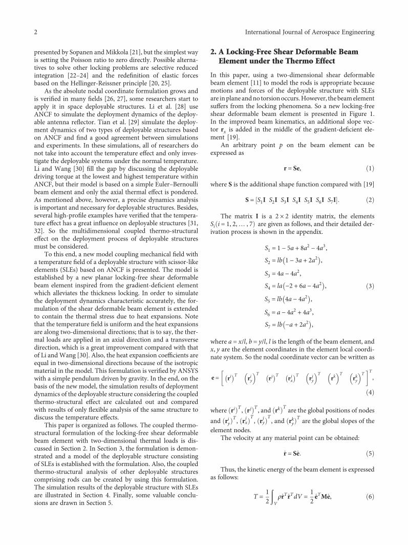
A simple example that a rectangular pendulum moves fromthe horizontal rest position under the effect of gravity(g = 9 8m/s2), as shown in Figure 2, is examined to validatethe proposed model with a two-dimensional thermal loadbased on ANCF. And the thermal load is applied by changingthe temperature from 0°C to 200°C suddenly. And other sim-ulation parameters such as the material property and geom-etry size of the pendulum are given in Table 1.

Figure 3 shows the curves of displacement of point awhich are evaluated by ANSYS, the 1D thermo-structuralmodel [30], and the proposed model, respectively. The twomodels are in good agreement with ANSYS within a largeoverall motion. It demonstrates that the proposed beamelement is free of locking phenomena. Further, in order toobserve the difference among three results clearly, a margincalculation is carried out. The difference between ANSYSand the flexible model, the difference between the 1Dthermo-structural model and the flexible model, and the dif-ference between the proposed model and the flexible modelare compared in Figure 4. Here, the flexible model impliesno temperature effect. It is clear from the difference valuepresent in Figure 4 that the proposed model is in good agree-ment with ANSYS, whereas the 1D thermo-structural modelhas a huge gap with ANSYS. So the proposed model hashigher precision. Therefore, the development of the newtwo-dimensional thermo-structural model is significant.

So the proposed model is used to assemble the deployablestructure with SLEs under the thermal effect. The dynamicsequations with the constraint conditions can be expressedas follows:

mq + k ΔT q +Φqλ = f ,Φ q, t = 0,

23

where q is the generalized coordinate vector of the deployablestructure, m and k are the mass matrix and the stiffnessmatrix, respectively, f is the generalized force vector, λ isthe Lagrange multipliers, Φ is the constraint equation, andΦq is the derivative matrix of Φ with respect to q. Note thatthe stiffness matrix k is the function of the temperature Tbesides the generalized coordinate vector q.

Y

X Point A

g

Figure 2: Planar rectangular pendulum with a change of thetemperature field.

4 International Journal of Aerospace Engineering

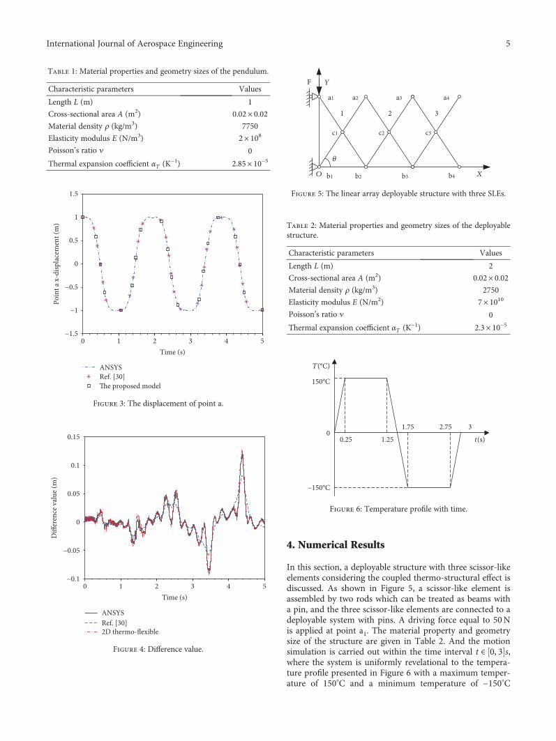
4. Numerical Results

In this section, a deployable structure with three scissor-likeelements considering the coupled thermo-structural effect isdiscussed. As shown in Figure 5, a scissor-like element isassembled by two rods which can be treated as beams witha pin, and the three scissor-like elements are connected to adeployable system with pins. A driving force equal to 50Nis applied at point a1. The material property and geometrysize of the structure are given in Table 2. And the motionsimulation is carried out within the time interval t ∈ 0, 3 s,where the system is uniformly revelational to the tempera-ture profile presented in Figure 6 with a maximum temper-ature of 150°C and a minimum temperature of −150°C

Table 1: Material properties and geometry sizes of the pendulum.

Characteristic parameters Values

Length L (m) 1

Cross-sectional area A (m2) 0.02× 0.02Material density ρ (kg/m3) 7750

Elasticity modulus E (N/m3) 2× 108

Poisson’s ratio ν 0

Thermal expansion coefficient αT (K−1) 2.85× 10−5

0 1 2 3 4 5−1.5

−1

−0.5

0

0.5

1

1.5

Time (s)

Poin

t a x

-disp

lace

men

t (m

)

ANSYSRef. [30]The proposed model

Figure 3: The displacement of point a.

0 1 2 3 4 5−0.1

−0.05

0

0.05

0.1

0.15

Time (s)

Diff

eren

ce v

alue

(m)

ANSYSRef. [30]2D thermo-flexible

Figure 4: Difference value.

F

XO

𝜃

1 2

Y

3

a1 a2 a3 a4

b1 b2 b3 b4

c1 c2 c3

Figure 5: The linear array deployable structure with three SLEs.

Table 2: Material properties and geometry sizes of the deployablestructure.

Characteristic parameters Values

Length L (m) 2

Cross-sectional area A (m2) 0.02× 0.02Material density ρ (kg/m3) 2750

Elasticity modulus E (N/m2) 7× 1010

Poisson’s ratio ν 0

Thermal expansion coefficient αT (K−1) 2.3× 10−5

150°C

−150°C

T(°C)

t(s)0.25 1.25

1.75 2.75 30

Figure 6: Temperature profile with time.

5International Journal of Aerospace Engineering

[30]. In order to demonstrate the temperature influence onthe dynamics of the mechanism, the simulation results arecompared with the same system only considering the flex-ible effect.

Figure 7 shows the deflection curves of rod b1a2, rod b2a3,and rod b3a4 in the changing temperature field as shown inFigure 6 and in the constant temperature field. Referring toFigure 7, it can be seen that the time-dependent tempera-ture leads to many small vibrations which can be observed2.7 s after clearly when the two curves differ greatly atthe moment. These small vibrations which will influencethe deployment accuracy greatly arise because thermallyinduced transverse strain results in varying moment of iner-tia related to the cross-sectional area besides the change of

the length of rods resulting from thermally induced axialstress. Another notable point from the pictures is that thetemperature influence on the deflection of the rods seemsto weaken in this time period of 2 s to 2.5 s. A probable rea-son is that the lowest temperature effect on the deployablestructure partly offsets the highest temperature effect in theearlier period.

The motion diagrams of a representative point a4 selectedto stand for the dynamics characteristics of the deployablestructure are shown in Figure 8. Referring to Figure 8, thetemperature impacting on deployment displacement andvelocity is not obvious, but there is a huge influence ondeployment acceleration of point a4. The thermal effectresults in additional vibrations emerging in acceleration,

0 0.5 1 1.5 2 2.5 3−0.01

0

0.01

0.02

0.03

0.04

0.05

0.06

0.07

Time (s)

Rod

b1a2

defl

ectio

n (m

)

FlexibleThermo-flexible

(a) Rod b1a2 deflection with time

0 0.5 1 1.5 2 2.5 3−0.005

0

0.005

0.01

0.015

0.02

0.025

0.03

Time (s)

Rod

b2a3

defl

ectio

n (m

)

FlexibleThermo-flexible

(b) Rod b2a3 deflection with time

0 0.5 1 1.5 2 2.5 3−6

−4

−2

0

2

4

6

8

10

12×10−3

Time (s)

Rod

b3a4

defl

ectio

n (m

)

FlexibleThermo-flexible

(c) Rod b3a4 deflection with time

Figure 7: Temperature effect on the deflection of rods.

6 International Journal of Aerospace Engineering

which can be observed by comparing the thermo-flexiblecurve with the flexible curve. Besides, referring to Figures 6and 8(c), it is found that acceleration vibrations becomelarger perspicuously at inflection points of the temperatureprofile such as 0.25 s, 1.25 s, 1.75 s, and 2.75 s. These vibra-tions may lead to unexpected collision and impact whichmight result in the invalidation of the deployable structureor even mission failure.

5. Conclusions

In this paper, the dynamics analysis of the deployable struc-ture with three SLEs considering the coupled thermo-structural effect based on ANCF is presented.

(1) In order to establish the precise model coupling of themechanical field with the temperature field of themechanism, the formulation of a new locking-freebeam element with the additional slope vector isextended to account for the thermally inducedstresses in two-dimensional directions, that is, theaxial direction and transverse direction

(2) It shows that the new beam element is free of lockingphenomena as a result of a good agreement betweenthe calculating results of the simple pendulum andthe simulation results of the ANSYS within a largeoverall motion. Then, the validity and the precisionof the proposed thermo-structural model are demon-strated through the further margin calculation: the

0 0.5 1 1.5 2 2.5 30.5

1

1.5

2

Time (s)

Poin

t a4

y-di

spla

cem

ent (

m)

Thermo-flexibleFlexible

1.3 1.4 1.5 1.6 1.7

1.8

1.85

1.9

1.95

2

(a) Displacement with time

Thermo-flexibleFlexible

0 0.5 1 1.5 2 2.5 3−5

−4

−3

−2

−1

0

1

Time (s)

Poin

t a4

y-ve

loci

ty (m

/s)

1.24 1.25 1.26−0.12

−0.1

−0.08

0.24 0.26

−0.04−0.02

00.02

1.75 1.755 1.76

−0.28

−0.27

−0.26

2.745 2.75 2.755−1.44

−1.43

−1.42

(b) Velocity with time

Thermo-flexibleFlexible

0 0.5 1 1.5 2 2.5 3−40

−30

−20

−10

0

10

20

30

Time (s)

Poin

t a4

y-ac

cele

ratio

n (m

/s2 )

(c) Acceleration with time

Figure 8: Deployment dynamics characteristics of the mechanism.

7International Journal of Aerospace Engineering

difference of the proposed model is approximatelyidentical to the difference of ANSYS, whereas thedifference of the 1D thermo-structural model has arelatively large gap with the difference of ANSYS.Therefore, the proposed model is more precise thanthe 1D thermal-structural model. On the otherhand, it also demonstrates that the development ofthe new two-dimensional thermo-structural modelis significant

(3) In the final simulations of the deployable structure,by contrasting the thermo-flexible deflection withthe flexible deflection, it is found that the maininfluence of temperature is that the change of tem-perature leads to many vibrations: for the deflectionof rods, many small vibrations arise because ther-mally induced transverse strain results in varyingmoment of inertia related to the cross-sectional areabesides the change of the length of rods resultingfrom thermally induced axial stress. On the otherhand, for the deployment dynamics characteristics,temperature has a huge impact on deploymentacceleration. The thermal effect will result in addi-tional vibrations emerging in acceleration of an arbi-trary point on the deployable structure, and thesevibrations will become larger perspicuously at inflec-tion points of temperature change

Appendix

For the new beam element, the displacement field isdefined as

r x, y =a0 + a1x + a2y + a3xy + a4x

2 + a5x3 + a6x

2y

b0 + b1x + b2y + b3xy + b4x2 + b5x

3 + b6x2y

,

A 1

where ai, bi i = 1, 2,⋯, 7 are the polynomial coefficients.The nodal displacement conditions shown in Figure 1

can be expressed as

r 0, 0 = ri,ry 0, 0 = riy ,

r l, 0 = rk,

ry l, 0 = rky ,

r l2 , 0 = rj,

rxl2 , 0 = rjx,

ryl2 , 0 = rjy

A 2

Thus, the polynomial coefficients can be derived from(A.2):

a0

b0= ri,

a1

b1= −

5ri − 4rj − rk + 2lrjxl

,

a2

b2= riy ,

a3

b3= −

3riy − 4rjy + rkyl

,

a4

b4= 8ri − 4rj − 4rk + 6lrjx

l2,

a5

b5= −

4ri − 4rk + 4lrjxl3

,

a6

b6=2riy − 4rjy + 2rky

l2

A 3

By substituting (A.3) into (A.1), the displacement field isrewritten with nodal displacement:

r x, y = 1 − 5a + 8a2 − 4a3 ri + lb 1 − 3a + 2a2 riy+ 4a − 4a2 rj + la −2 + 6a − 4a2 rjx+ lb 4a − 4a2 rjy + a − 4a2 + 4a3 rk

+ lb −a + 2a2 rky = Se,A 4

where

e = ri T riyT

rj T rjxT rjy

Trk

Trky

TT

,

S = S1I S2I S3I S4I S5I S6I S7I ,S1 = 1 − 5a + 8a2 − 4a3,S2 = lb 1 − 3a + 2a2 ,

S3 = 4a − 4a2,S4 = la −2 + 6a − 4a2 ,

S5 = lb 4a − 4a2 ,

S6 = a − 4a2 + 4a3,S7 = lb −a + 2a2

A 5

8 International Journal of Aerospace Engineering

Data Availability

The data that support the findings of this study are availablefrom the corresponding author upon reasonable request.

Conflicts of Interest

The authors declared no potential conflicts of interest withrespect to the research, authorship, and/or publication ofthis article.

Acknowledgments

This work was supported by the National Natural ScienceFoundation of China (grant number 51175422).

References

[1] Z. You and S. Pellegrino, “Deployable mesh reflector,” TheInternational Symposium on Spatial, Lattice, and TensionStructures, pp. 103–112, 1994.

[2] A. G. Cherniavsky, V. I. Gulyayev, V. V. Gaidaichuk, and A. I.Fedoseev, “Large deployable space antennas based on usage ofpolygonal pantograph,” Journal of Aerospace Engineering,vol. 18, no. 3, pp. 139–145, 2005.

[3] Y. Wang, R. Liu, H. Yang, Q. Cong, and H. Guo, “Design anddeployment analysis of modular deployable structure for largeantennas,” Journal of Spacecraft and Rockets, vol. 52, no. 4,pp. 1101–1111, 2015.

[4] B. Li, S. M. Wang, R. Yuan, X. Z. Xue, and C. J. Zhi, “Dynamiccharacteristics of planar linear array deployable structurebased on scissor-like element with joint clearance using anew mixed contact force model,” Proceedings of the Institutionof Mechanical Engineers, Part C: Journal of Mechanical Engi-neering Science, vol. 230, no. 18, pp. 3161–3174, 2016.

[5] Y. Tang, T. Li, Z. Wang, and H. Deng, “Surface accuracy anal-ysis of large deployable antennas,” Acta Astronautica, vol. 104,no. 1, pp. 125–133, 2014.

[6] J. Sun, Q. Tian, and H. Hu, “Structural optimization of flexiblecomponents in a flexible multibody system modeled viaANCF,” Mechanism and Machine Theory, vol. 104, pp. 59–80, 2016.

[7] Y. Zhang, B. Duan, and T. Li, “A controlled deploymentmethod for flexible deployable space antennas,” Acta Astro-nautica, vol. 81, no. 1, pp. 19–29, 2012.

[8] J. García de Jalón and E. Bayo, Kinematic and Dynamic Simu-lation of Multibody Systems, Mechanical Engineering Series,Springer, New York, 1994.

[9] A. A. Shabana, Dynamics of Multibody Systems, CambridgeUniversity Press, 2005.

[10] M. Berzeri and A. A. Shabana, “Study of the centrifugal stiffen-ing effect using the finite element absolute nodal coordinateformulation,” Multibody System Dynamics, vol. 7, no. 4,pp. 357–387, 2002.

[11] M. A. Omar and A. A. Shabana, “A two-dimensional sheardeformable beam for large rotation and deformation prob-lems,” Journal of Sound and Vibration, vol. 243, no. 3,pp. 565–576, 2001.

[12] A. A. Shabana, Computational Continuum Mechanics,Cambridge University Press, 2012.

[13] M. Berzeri and A. A. Shabana, “Development of simple modelsfor the elastic forces in the absolute nodal co-ordinate formu-lation,” Journal of Sound and Vibration, vol. 235, no. 4,pp. 539–565, 2000.

[14] A. A. Shabana and R. Y. Yakoub, “Three dimensional absolutenodal coordinate formulation for beam elements: theory,”Journal of Mechanical Design, vol. 123, no. 4, pp. 606–613,2001.

[15] R. Y. Yakoub and A. A. Shabana, “Three dimensional absolutenodal coordinate formulation for beam elements: implementa-tion and applications,” Journal of Mechanical Design, vol. 123,no. 4, pp. 614–621, 2001.

[16] S. von Dombrowski, “Analysis of large flexible body deforma-tion in multibody systems using absolute coordinates,” Multi-body System Dynamics, vol. 8, no. 4, pp. 409–432, 2002.

[17] O. N. Dmitrochenko and D. Y. Pogorelov, “Generalization ofplate finite elements for absolute nodal coordinate formula-tion,” Multibody System Dynamics, vol. 10, no. 1, pp. 17–43,2003.

[18] L. Kübler, P. Eberhard, and J. Geisler, “Flexible multibody sys-tems with large deformations using absolute nodal coordinatesfor isoparametric solid brick elements,” in ASME 2003 Inter-national Design Engineering Technical Conferences and Com-puters and Information in Engineering Conference, pp. 31–52,Chicago, Illinois, USA, September 2003.

[19] D. García-Vallejo, A. M. Mikkola, and J. L. Escalona, “A newlocking-free shear deformable finite element based on absolutenodal coordinates,” Nonlinear Dynamics, vol. 50, no. 1-2,pp. 249–264, 2007.

[20] B. A. Hussein, H. Sugiyama, and A. A. Shabana, “Coupleddeformation modes in the large deformation finite-elementanalysis: problem definition,” Journal of Computational andNonlinear Dynamics, vol. 2, no. 2, p. 146, 2007.

[21] J. T. Sopanen and A. M. Mikkola, “Description of elastic forcesin absolute nodal coordinate formulation,” Nonlinear Dynam-ics, vol. 34, no. 1/2, pp. 53–74, 2003.

[22] K. S. Kerkkänen, J. T. Sopanen, and A. M. Mikkola, “A linearbeam finite element based on the absolute nodal coordinateformulation,” Journal of Mechanical Design, vol. 127, no. 4,pp. 621–630, 2005.

[23] J. Gerstmayr, M. K. Matikainen, and A. M. Mikkola, “Ageometrically exact beam element based on the absolutenodal coordinate formulation,” Multibody System Dynamics,vol. 20, no. 4, pp. 359–384, 2008.

[24] K. Nachbagauer, A. S. Pechstein, H. Irschik, and J. Gerstmayr,“A new locking-free formulation for planar, shear deformable,linear and quadratic beam finite elements based on the abso-lute nodal coordinate formulation,”Multibody System Dynam-ics, vol. 26, no. 3, pp. 245–263, 2011.

[25] H. Sugiyama and Y. Suda, “A curved beam element in the anal-ysis of flexible multi-body systems using the absolute nodalcoordinates,” Proceedings of the Institution of MechanicalEngineers, Part K: Journal of Multi-body Dynamics, vol. 221,no. 2, pp. 219–231, 2007.

[26] W. S. Yoo, J. H. Lee, S. J. Park, J. H. Sohn, D. Pogorelov, andO. Dmitrochenko, “Large deflection analysis of a thin plate:computer simulations and experiments,” Multibody SystemDynamics, vol. 11, no. 2, pp. 185–208, 2004.

[27] W. S. Yoo, M. S. Kim, S. H. Mun, and J. H. Sohn, “Largedisplacement of beam with base motion: flexible multibodysimulations and experiments,” Computer Methods in Applied

9International Journal of Aerospace Engineering

Mechanics and Engineering, vol. 195, no. 50-51, pp. 7036–7051, 2006.

[28] P. Li, C. Liu, Q. Tian, H. Hu, and Y. Song, “Dynamics of adeployable mesh reflector of satellite antenna: parallel compu-tation and deployment simulation 1,” Journal of Computa-tional and Nonlinear Dynamics, vol. 11, no. 6, article 061005,2016.

[29] Q. Tian, J. Zhao, C. Liu, C. Zhou, and H. Hu, “Dynamics ofspace deployable structures,” in ASME 2015 InternationalDesign Engineering Technical Conferences and Computersand Information in Engineering Conference, ASME, Boston,USA, 2015.

[30] T. Li and Y. Wang, “Deployment dynamic analysis of deploy-able antennas considering thermal effect,” Aerospace Scienceand Technology, vol. 13, no. 4-5, pp. 210–215, 2009.

[31] E. Thornton and R. Foster, “Dynamic response of rapidlyheated space structures,” in Computational NonlinearMechanics in Aerospace Engineering, pp. 451–477, 33rd Struc-tures, Structural Dynamics and Materials Conference, Dallas,TX, USA, 2013.

[32] C. L. Foster, M. L. Tinker, G. S. Nurre, and W. A. Till, “Solar-array-induced disturbance of the Hubble Space Telescopepointing system,” Journal of Spacecraft and Rockets, vol. 32,no. 4, pp. 634–644, 1995.

[33] B. A. Boley, J. H. Weiner, and E. H. Dill, “Theory of thermalstresses,” Physics Today, vol. 14, no. 3, pp. 58–60, 1961.

10 International Journal of Aerospace Engineering

International Journal of

AerospaceEngineeringHindawiwww.hindawi.com Volume 2018

RoboticsJournal of

Hindawiwww.hindawi.com Volume 2018

Hindawiwww.hindawi.com Volume 2018

Active and Passive Electronic Components

VLSI Design

Hindawiwww.hindawi.com Volume 2018

Hindawiwww.hindawi.com Volume 2018

Shock and Vibration

Hindawiwww.hindawi.com Volume 2018

Civil EngineeringAdvances in

Acoustics and VibrationAdvances in

Hindawiwww.hindawi.com Volume 2018

Hindawiwww.hindawi.com Volume 2018

Electrical and Computer Engineering

Journal of

Advances inOptoElectronics

Hindawiwww.hindawi.com

Volume 2018

Hindawi Publishing Corporation http://www.hindawi.com Volume 2013Hindawiwww.hindawi.com

The Scientific World Journal

Volume 2018

Control Scienceand Engineering

Journal of

Hindawiwww.hindawi.com Volume 2018

Hindawiwww.hindawi.com

Journal ofEngineeringVolume 2018

SensorsJournal of

Hindawiwww.hindawi.com Volume 2018

International Journal of

RotatingMachinery

Hindawiwww.hindawi.com Volume 2018

Modelling &Simulationin EngineeringHindawiwww.hindawi.com Volume 2018

Hindawiwww.hindawi.com Volume 2018

Chemical EngineeringInternational Journal of Antennas and

Propagation

International Journal of

Hindawiwww.hindawi.com Volume 2018

Hindawiwww.hindawi.com Volume 2018

Navigation and Observation

International Journal of

Hindawi

www.hindawi.com Volume 2018

Advances in

Multimedia

Submit your manuscripts atwww.hindawi.com