dynamics and composition measurements with the...

Dynamics and Composition Measurements with the Purple Crow Lidar 1

r- ,

heceeareentae

ufil-no

malla

mthciodeinW

w

-n

tro-dle theer-d-ntdlere-

eral

urbedu-wericfol-ityea-Wewerew

arpera-ium

Dynamics and Composition Measurements in the Lower and Middle Atmosphere with the Purple Crow Lidar

R. J. Sica, P. S. Argall, A. T. Russell, C. R. Bryant* and M. M. Mwangi**Department of Physics and Astronomy, The University of Western Ontario, London, Ontario, Canada N6A [email protected]

*Now at Department of Physics and Astronomy, University of Calgary, Alberta, Canada**Now at Department of Physics, Cornell University, Ithaca, NY, U.S.A.

ABSTRACT

The Purple Crow Lidar (PCL) is a large power-apeture product monostatic laser radar which has beenoperation at the Delaware Observatory (

, 225 m elevation above sea level) near tcampus of The University of Western Ontario sin1992. The PCL is capable of making simultaneous msurements of Rayleigh, Raman and resonance fluocence scattering, which allows temperature, constitudensity and gravity wave parameters to be simulneously determined from the troposphere to the lowthermosphere. Temperature measurements are of scient accuracy to identify layers of stability and instabity in the middle atmosphere. Density fluctuatiomeasurements throughout the lower and middle atmsphere can be used to estimate the spectrum of atspheric gravity waves at high spatial-temporresolution. We have used these measurements to isoindividual waves in the vertical wavenumber spectruto determine eddy diffusion profiles and to measure temporal spectrum in the stratosphere past the lobuoyancy frequency. We have also begun compositmeasurements, including the first routine mid-latituground-based measurements of water vapour mixratio from near the surface to the lower stratosphere. have also developed and applied a new techniqueallow N2 and O2 density profiles to be estimated fromPCL measurements in the upper mesosphere and lothermosphere.

42°52′ N81°23′ W

in

-s-t

-rfi-

-o-

te,ealn

geto

er

I. INTRODUCTION

The fundamental meteorological quantities of temperature, density, wind and humidity are well knownear the surface and reasonably well known in the posphere. However, weather variables in the midatmosphere, e.g. the region above the troposphere toturbopause (10 to 115 km) are much more poorly undstood. It is clear, however, that general circulation moels in the lower atmosphere show significaimprovement when they are extended into the midatmosphere. Hence, it is important to make measuments which can be used to test the reality of gencirculation models.

PCL measurements which have improved ounderstanding of the middle atmosphere are descriin this review. First, a description of the system configration and hardware is given, followed by an overvieof our temperature measurements. The mesosphinversion layers are then discussed in some detail, lowed by a summary of our results concerning gravwaves and superadiabatic layering. Composition msurements are discussed in the final two sections. describe our measurements of troposphere and lostratospheric water vapour and then introduce a ntechnique which allows the determination of N2 and O2altitude profiles from concurrent Rayleigh-scatter lidbackscatter measurements and an independent temture determination such as those obtained from sodresonance fluorescence scattering measurements.


rat

as

erm

thoangintmlidth

areedac-r ae

inosnanrs

ghovictte isaethemhtte

helityamc-f

rory-

s-oreer.ea-

m-.

nedsandhe Naz)

tois

ou-seis

ld-

tog-ler-the

Current information about the PCL, including coloversions of many of the following figures, is available our web site (http://pcl.physics.uwo.ca).

II. PCL SYSTEM DESCRIPTION

The hardware for an atmospheric lidar system cbe conveniently divided into two components, the tranmitter and the receiver. The transmitter of a lidar genally consists of a pulsed laser system with beaexpanding optics and steering mirrors that are useddirect the light into the sky. Once in the atmosphere laser light interacts with the constituents of the atmsphere and a portion of the emitted laser photons scattered back to the lidar receiving system. By utilizia variety of laser wavelengths, atmospheric scatterprocesses and detection techniques, a number of aspheric parameters can be measured using the technique. The transmitter and receiver systems for PCL are described below.

II.1. PCL TransmitterThe type of laser system employed in a lid

depends in large part on the quantity the lidar has bdesigned to measure. Rayleigh and Raman-scatter liutilize the forms of scattering implied by their respetive names. Both these forms of scattering occur ovewide range of wavelengths and so do not require a pticular laser wavelength. The choice of the type of lasto be used in a Rayleigh-Raman lidar needs to take account many factors including the backscatter crsection at the laser wavelength, the atmospheric tramission at the laser wavelength, the ease of use affordability of the laser and the efficiency of detectoat the detection wavelength.

The laser used in the transmitter for the Rayleiand Raman channels of the PCL to optimize the abtrade-offs is a frequency doubled Nd:YAG. The basparameters of the PCL Rayleigh and Raman transmiis summarized in Table 1. The output of this laserexpanded in order to reduce the divergence of the beand transmitted vertically into the sky coaxially with threceiving telescope. Reducing the divergence of transmitted laser beam allows the field-of-view of thdetection system to be reduced, which lowers the nuber of multiply scattered photons, scattered moon ligstar light and anthropogenic sources which are detecas a background.

Transmitting the laser beam along the axis of tdetection telescope significantly reduces the possibiof an overlap error in the alignment of the laser beand the field-of-view of the detection system. If the fration of the laser beam that is within the field-of-view o

n--

toe-re

go-are

nrs

ar-rtoss-d

e

r

m

e

-,d

the detection system changes with altitude an erwould result in the temperatures derived from the Raleigh lidar.

The transmitter for the sodium-resonance-fluorecence system (henceforth the Na system) is much mcomplex than that of the Rayleigh-Raman transmittThe Na lidar temperature measurements require msurements of the spectral width of the Na D2a line. Thismeasured line width is then used to determine the teperature of the mesopause region of the atmosphere

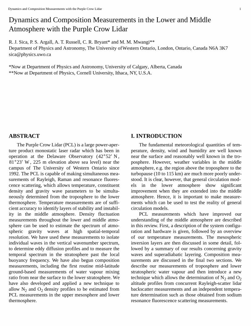
In order to measure the Na D2a line’s spectral widththe PCL uses a narrow line width laser that can be tuacross the Na D2a line. A combination of several laseris required to produce the pulsed, tunable, narrow-band relatively high power light source required for tNa lidar temperature measurements (Figure 1). Thetransmitter comprises a tunable narrow-band (500 kHring-dye-laser (RDL) which is pumped by an Ar+ laseroperating at 4 W. The cw beam from the RDL is usedseed a 3 stage pulsed-dye-amplifier (PDA) which pumped by a 600 mJ per pulse, 20 Hz frequency dbled Nd:YAG beam. The PDA output is 6 0mJ per pulat 20 Hz with a spectral width of about 106 kHz. Thbeam is expanded to a diameter of 2 7mm and transmit-ted into the sky coaxially with the detector system fieof-view.

A sample of the output of the RDL is directed inthe ring-laser-frequency-control-system (RLFCS; Fiure 1). The RLFCS uses a technique known as Doppfree-saturation-spectroscopy (DFSS) to actively lock

Table 1. Specifications of the PCL Rayleigh and Ramantransmitter.

Wavelength 532 nm

Energy per pulse 600 mJ

Repetition rate 20 Hz

Pulse length 7 ns FWHM

Beam diameter 27 mm

Beam divergence at e-2 0.2 mrad, full width

Figure 1. Schematic of the PCL transmitter system.

Ring-dye-laser Ar+ laser

Ring laser frequencycontrol system

Nd:YAGAm plifier

Freq.Doubler

Nd:YAGAm plifier

Nd:YAGAm plifier

Freq.Doubler

Nd:YAGOscillatorSeeder

PDACell 1

PDACell 3

PDACell 2

BeamExpander

BeamExpander

SpectrumAnalyser

Pulsed-Dye-Am plifier


is

l-

ahom on ntic-enthveenni

to

)ps.tour

nure

cat-ve

isfi-lti-m

ene

ofrstiongh

n-c,s).n-

larsof

Lo-on notels

-u-se

calmis

eda-the

at-

RDL’s output frequency to a frequency marker that generated by a cell containing Na vapour. The frequencymarkers that are generated using this techniquewithin the Na D2a line. Further details of the narrowband Na technique and the use of DFSS are foundArgall et al. (1) and the references therein.

II.2. PCL ReceiverThe receiving system for the PCL is based on

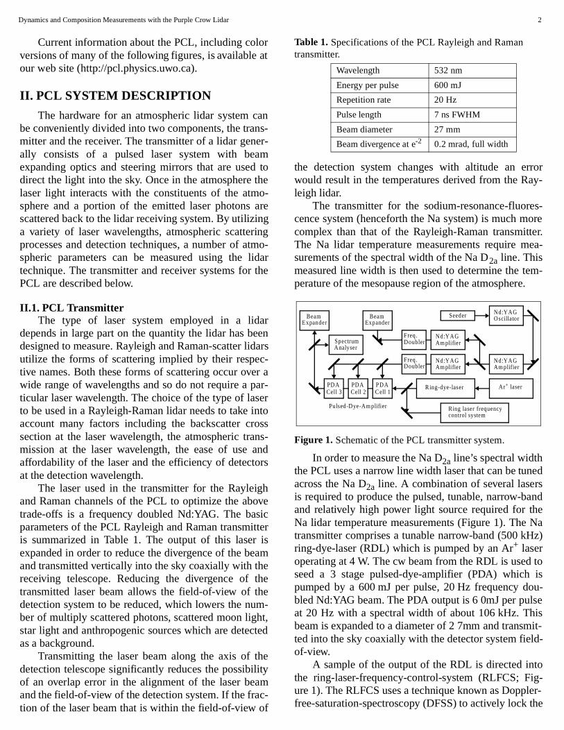
2.65 m diameter liquid mirror telescope (LMT), whicis described by Sica et al. (2). Light backscattered frthe atmosphere is focused by the LMT onto the planethe entrance aperture of the detection system showFigure 2. Light that is reflected from the LMT thepasses through the entrance aperture of the detecsystem and is collimated by lens L1. The dichroibeam-splitter, DBS1, reflects the two Raman wavlengths of interest for water vapour measurements oDBS2 which reflects the nitrogen Raman waveleng(607 nm) and transmits the water vapour Raman walength (660 nm). Light at these two wavelengths is thincident on 1.0 nm bandwidth interference filters, cetered at the appropriate wavelengths. The light transmted by the interference filters is focused onphotomultiplier tubes.

Light at the Rayleigh (532 nm) and Na (589 nmwavelengths is transmitted by DBS1 to a rotating choper which removes low altitude (below 25 km) returnLight transmitted by the chopper is split by DBS3 inRayleigh and Na beams. These two beams pass thro1.0 nm interference filters and onto photomultiplie

Figure 2. Schematic of the PCL detector system.

R ayle igh 532 nm

S odium 532 nm

N itrogen 607 nm

W ater vapour660 nm

M otor

Chopper

P hotom ultip lierH ousings

IF

IF

IF

IF

M

D BS 1D B S2

D B S3

L1

L 2

L3

From L M T

Entrance aperture

IF In terference F ilterM M irrorD B S# D ichroic beam splitterL# L ens - achrom atic doublet

ie

in

fin

on

-to

-

-t-

-

gh

tubes. All four photomultipliers used in this detectiosystem are Hamamatsu model R5600P-01 miniatphotomultipliers.

The PCL Raman system ratios the Raman backster from water vapour and molecular nitrogen to achiea measurement of the water vapour mixing ratio. Ittherefore important that the ratio of the optical efciency of these two channels does not change with atude. Careful optical design of the receiver systeensures that this ratio is constant with altitude.

The optics of the PCL detector system have bedesigned so that the LMT forms the limiting pupil of thsystem and the entrance aperture of the detector housingforms the limiting aperture (Figure 2). This choice limiting pupil guarantees that no vignetting occuinside the detector housing. Thus, each of the detecchannels sees exactly the same field-of-view throuexactly the same pupil.

The two Raman channel photomultipliers are conected via 300 MHz discriminators (Phillips Scientifi6904) to PC-card type multichannel scalars (NucleuThe Rayleigh and Na channel photomultipliers are conected to Stanford Research multichannel sca(SR 430) which have a maximum count rate 100 MHz.

Due to the high power-aperture product of the PCsignificant nonlinearities in the counting of the photmultiplier pulses occurs for three of the four detectichannels. The Raman water vapour channel doessuffer from this problem because of the low signal levin this channel.

Using a light-emitting-diode (LED) and signal generator an optical signal resembling the intensity distribtion of the actual lidar returns can be simulated. Thesimulated returns, measured with and without an optiattenuator, allow a correction for the counting systenonlinearities to be determined. This correction applied to the atmospheric backscatter measurements aspart of the data reduction.

III. Temperature Results

III.1. Rayleigh TemperatureThe Rayleigh lidar technique is a well establish

method for providing high resolution temperature mesurement from the middle of the stratosphere up to lower thermosphere (2,3).

A Rayleigh lidar measures the number of backsctered laser photons as a function of altitude, i.e.

, (1)N z( ) Cn z( )z2----------=


h nga

eno

de rena

inrelti-ethfileto athaitur-nntresemch

ill

eaha

tee

esti--thd

thur

ch toric

sig-

ion toes-hisofout

a-0 tom-, asnty-om-notd be

totionesetheen-d

ionnts,canhe

ghratere-nd-kyCLthe

st)em-ghs is-

ofomdelsticherer

entshe

where N is the number of photons detected, z is the alti-tude, n is the atmospheric number density and C is aconstant that includes the effects of parameters suclaser power, detector system efficiency and collectiarea, transmission of the lower atmosphere and the Rleigh backscatter cross section of air.

The calibration constant, C, in Equation 1 cannot bedetermined precisely due to uncertainties in instrumtal parameters and the transmission of the lower atmsphere. Thus, N(z) is a relative density profile. Thisrelative density profile can be scaled using a moatmosphere, over an extended altitude range, so it issonably well scaled. However, temperature determitions only require a relative density profile.

Temperature is found from the relative density usthe Ideal Gas Law and assuming that the atmosphein hydrostatic equilibrium, i.e. the pressure at any atude is equal to the weight of the air above that levChanin et. al. (3) and Shibata et. al. (4) describe details of calculating an absolute temperature profrom a relative density profile. Using this method determine an absolute temperature profile requiresestimate of the actual temperature or pressure at uppermost altitude at which measurements are avable. This estimate is required to seed the temperaretrieval integration algorithm. Of course, this uncetainty can be eliminated if the temperature is knowThe coincident PCL Na temperature lidar measuremeoffer the possibility of making absolute temperatumeasurements in this region, which could then be uto seed the Rayleigh temperature retrieval algorithArgall et al. have shown some initial results of sutemperature seeding (1).

An error in the initial temperature (pressure) wmanifest itself as an error in the calculated absolute tem-perature profile. Generally, absolute temperature msurements made coincidently with Rayleigmeasurements at 100 to 110 km are generally not avable and model atmospheres are used to initiate the perature retrieval algorithm. The magnitude of thinitialization error in the temperature retrieval reducquickly as the integration progress downward in altude. An error of 10 K in the estimate of the initial temperature is reduces to less than 3 K at 10 km below initialization altitude. All of the temperatures presentehere have been calculated from temperature profiles have had the top 10 km removed. This procedensures that the measurements presented are not signifi-cantly influenced by this initialization effect.

The Rayleigh lidar temperature measurement tenique works in the altitude range of approximately 25100 km. Below 25 km scattering from the stratosphe

as

y-

--

la--

g is

l.e

nel-re

.s

d.

-

il-m-

e

ate

-

aerosol layer contaminates the measured Rayleigh nal and cannot be removed without very precise spectralmeasurements of the backscattered light. A correctfor the optical transmission of the atmosphere dueozone in the altitude range of 25 to 50 km is also necsary for the temperature retrievals. Corrections for teffect are given by Sica et. al. (5). The application this correction leads to a temperature difference of ab0.5 K at 30 km and is wavelength dependent.

The upper altitude limit for the Rayleigh temperture technique is generally considered to be about 10110 km. This altitude limit is based both upon the coposition changes that occur above these altitudeswell as the signal-to-noise ratio limitations of curreRayleigh lidars. The uncertainties introduced into Raleigh lidar temperature measurements because of cposition changes in the lower thermosphere are addressed in the current analysis scheme, but shoulconsidered in the future (see Section VII).

Changes in atmospheric composition leads changes in both the Rayleigh backscatter cross secand the mean molecular mass of air. Changes in thtwo parameters must to be taken into account in Rayleigh temperature retrievals at higher altitudes. Gerally this composition information is not available anso this type of correction may not be possible. SectVI discusses how the Rayleigh scatter measuremecombined with Na lidar temperature measurements, be used to determine composition information in taltitude range 85 to 105km.

The PCL has been routinely measuring Rayleitemperatures since early 1994 and continues to opeon most clear nights. The majority of the PCL measument are between mid spring and mid fall, correspoing to the time of year when the probability of clear sis greatest. Table 2 shows the distribution of the PRayleigh lidar temperature set. The bias toward summer months is obvious.

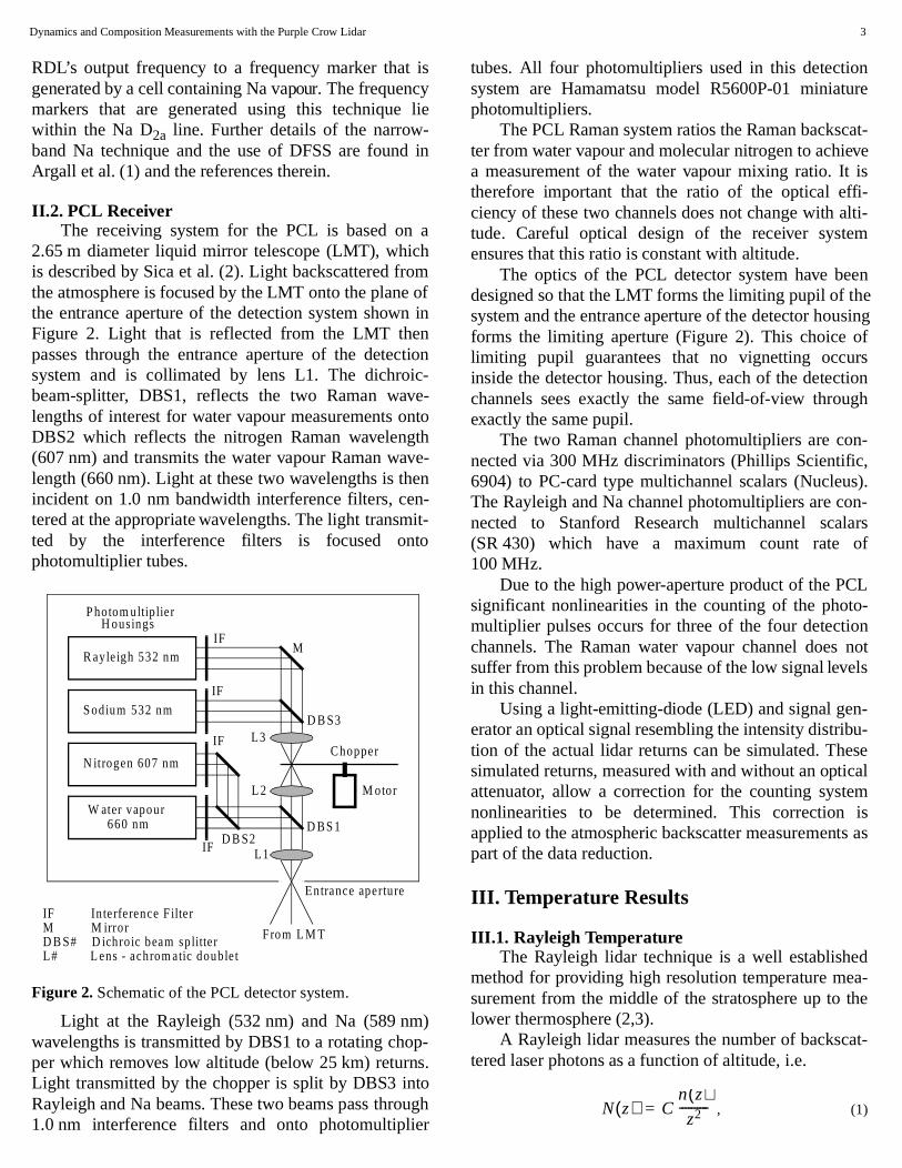
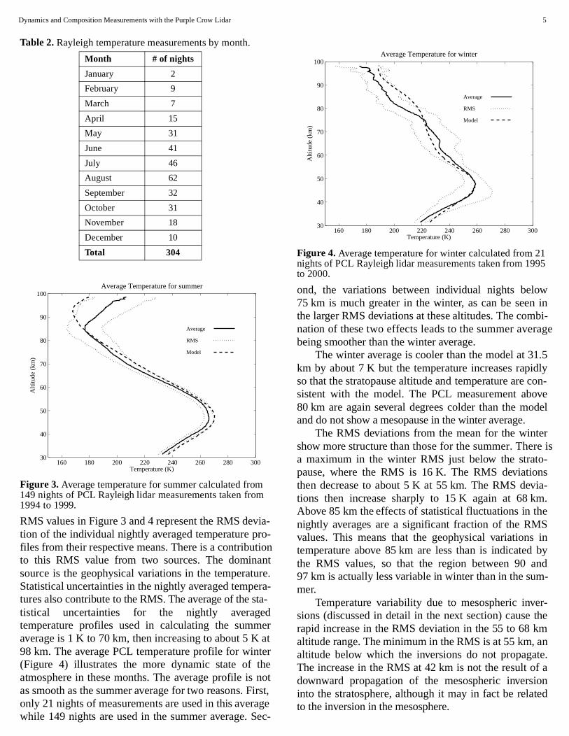
Figures 3 and 4 show summer (June, July, Auguand winter (December, January, February) average tperature profiles calculated from the PCL Rayleimeasurements. The average for the summer monthsignificantly lower than predicted by the model of Fleming et. al. (6) from 31.5 km to 74km. In fact, the sum the mean lidar temperature and the RMS deviation frthe mean is very similar to the temperature of the moover the entire range of 30 to 70km. However, the mostriking feature is the altitude of the mesopause, whis observed at 85 km. This height is about 7. 5km lowthan suggested by the Fleming et al. model. This lowsummer mesopause is in agreement with measuremobtained by Na lidar systems (e.g. Senft et. al. (7)). T


iao-ionrratade atehe nirage

wn inbi-rage

1.5dlycon-oveodel

erre iso-nsia-m.eS in bynd

m-

r- them

ante.f a

ionted

1 95

RMS values in Figure 3 and 4 represent the RMS devtion of the individual nightly averaged temperature prfiles from their respective means. There is a contributto this RMS value from two sources. The dominasource is the geophysical variations in the temperatuStatistical uncertainties in the nightly averaged tempetures also contribute to the RMS. The average of the stistical uncertainties for the nightly averagetemperature profiles used in calculating the summaverage is 1 K to 70 km, then increasing to about 5 K98 km. The average PCL temperature profile for win(Figure 4) illustrates the more dynamic state of tatmosphere in these months. The average profile isas smooth as the summer average for two reasons. Fonly 21 nights of measurements are used in this averwhile 149 nights are used in the summer average. S

Table 2. Rayleigh temperature measurements by month.

Month # of nights

January 2

February 9

March 7

April 15

May 31

June 41

July 46

August 62

September 32

October 31

November 18

December 10

Total 304

Figure 3. Average temperature for summer calculated from149 nights of PCL Rayleigh lidar measurements taken from 1994 to 1999.

160 180 200 220 240 260 280 30030

40

50

60

70

80

90

100

Temperature (K)

Alti

tude

(km

)

Average Temperature for summer

Average

RMS

Model

-

nte.--

rtr

otst,ec-

ond, the variations between individual nights belo75 km is much greater in the winter, as can be seethe larger RMS deviations at these altitudes. The comnation of these two effects leads to the summer avebeing smoother than the winter average.

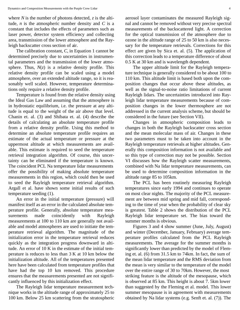
The winter average is cooler than the model at 3km by about 7 K but the temperature increases rapiso that the stratopause altitude and temperature are sistent with the model. The PCL measurement ab80 km are again several degrees colder than the mand do not show a mesopause in the winter average.

The RMS deviations from the mean for the wintshow more structure than those for the summer. Thea maximum in the winter RMS just below the stratpause, where the RMS is 16 K. The RMS deviatiothen decrease to about 5 K at 55 km. The RMS devtions then increase sharply to 15 K again at 68 kAbove 85 km the effects of statistical fluctuations in thnightly averages are a significant fraction of the RMvalues. This means that the geophysical variationstemperature above 85 km are less than is indicatedthe RMS values, so that the region between 90 a97 km is actually less variable in winter than in the sumer.

Temperature variability due to mesospheric invesions (discussed in detail in the next section) causerapid increase in the RMS deviation in the 55 to 68 kaltitude range. The minimum in the RMS is at 55 km, altitude below which the inversions do not propagaThe increase in the RMS at 42 km is not the result odownward propagation of the mesospheric inversinto the stratosphere, although it may in fact be relato the inversion in the mesosphere.

Figure 4. Average temperature for winter calculated from 2nights of PCL Rayleigh lidar measurements taken from 19to 2000.

160 180 200 220 240 260 280 30030

40

50

60

70

80

90

100

Temperature (K)

Alti

tude

(km

)

Average Temperature for winter

Average

RMS

Model


thomerre oio

s thred .e sly

thathisda

reoftemto

2

deicighfu

nd

entsevalheme ofeenos-

ecureb-onalareheareny

as

la-o-veix-

thathinhat12)therav-r-

letedheyra-ereseeris-nselti-er-ated

ishe atsi-

III.2. Sodium temperaturesThe Na lidar technique uses a measurement of

spectral shape of the resonantly scattered light frneutral Na atoms to determine the atmospheric tempture. A layer of Na atoms exists in the atmosphebetween about 85 and 105 km due to the depositionNa, as well as other metallic species, from the ablatof meteors at these altitudes.

Na lidar uses a laser that is tuned to the Na D2a line.Resonant scattering at this frequency is many ordermagnitude greater than that for Rayleigh scatter at same wavelength. This large cross section allows a sonable signal-to-noise measurements to be obtaineNa lidar despite the small amount of sodium present

To achieve a measurement of the spectral shapthe backscattered light from the Na layer the PCL tranmits alternately groups of pulses at two precisedefined wavelengths within the Na D2a line. The ratio ofthe intensity of the backscatter at these two wavelengis a measure of the line shape and can be directly relto the kinetic temperature. Further discussion of tmethod and a detailed error analysis of the PCL Na lisystem can be found in Argall et. al. (1).

Figure 5 shows the evolution of the temperatuprofile measured with the PCL Na lidar on the night May 21, 1998. This figure illustrates the dynamic staof the atmosphere in this region. At an altitude of 91 kthe temperature changes from 155 K at 0530 UT 200 K at 0715 UT, a change of 45 K in less thanhours.

Both the Rayleigh and Na lidar techniques provipowerful tools for remotely monitoring atmosphertemperature. Having a lidar able to make both Rayleand Na measurement simultaneously extends the use

Figure 5. Temperatures measurements at 8 min temporal a250 m vertical resolution made by the PCL Na resonance fluorescence lidar.

Tem

perature (K)

160

165

170

175

180

185

190

195

200

5 5.5 6 6.5 7 7.5 8 8.5

84

86

88

90

92

94

96

98

100

Time (UT)

Alti

tude

(km

)

e

a-

fn

ofea-by

of-

sed

r

l-

ness of both techniques. Na temperature measuremcan be used to seed the Rayleigh temperature retrialgorithm, improving the derived temperatures. Tcombination of the measurements also allows socomposition information to be obtained. One featurethe atmospheric temperature structure which has bstudied in some detail are inversion layers in the mesphere.

IV. MESOSPHERIC INVERSION LAYERS

It is well known that inversions with temperaturincreases on the order of tens of degrees routinely ocin the mesosphere and lower thermosphere (8,9). Llanc and Hauchecorne (10) have studied the seasvariations of inversions and found that the inversions stronger in the winter months at midlatitudes, while tinversions measured during the summer months strongest at lower latitudes. They also found that mainversions have an extended longitudinal structure,opposed to being a local phenomena.

What is the cause of these inversions? Most expnations of mesospheric inversion layers involve atmspheric waves, though Whiteway et al. (11) hasuggested that the inversions form due to turbulent ming in a manner similar to the formation of the planetaryboundary layer. Hauchecorne et al. (9) suggested the inversions are due to gravity waves breaking witthe inversion region for extended periods. Evidence ttides are also involved was presented by Dao et al. (and States and Gardner (13). Subsequently, Meriweet al. (14) have suggested that tidal modulation of grity wave forcing is the key to the formation of the invesions.

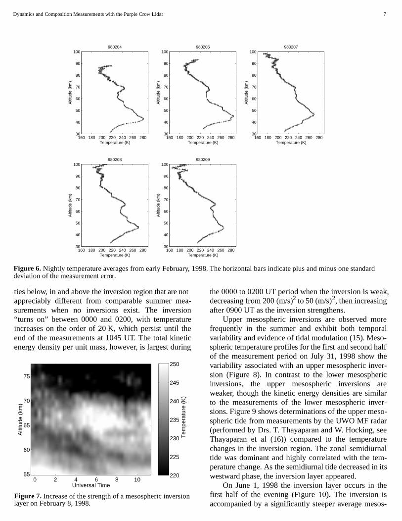
The high temporal-spatial resolution of the PurpCrow Lidar has revealed two new properties associawith mesospheric inversions. The first property is tvariability of these structures over time. While mannights show inversions in the nightly average, tempeture variations of 5 to 10% in the actual inversion layare not uncommon. The second property is that thinversions appear to exist in two distinct classes. Lowmesospheric inversions are the inversions typically dcussed in the literature. Lower mesospheric inversiopersist from night to night (Figure 6). However, in thsummer months the inversion occur frequently at atudes around 75 to 80 km. These higher altitude invsions are variable over a night and appear to be relto the tides.

The role of gravity waves in the inversion layers not directly evident from the PCL measurements. Tlower mesospheric inversion layer shown in Figure 765 km altitude is associated with kinetic energy den


oa

ionrehetiin

ak,

oreralo-

theer-ricareilarer-so-

dareeurenalm-n its

theisos-

Figure 6. Nightly temperature averages from early February, 1998. The horizontal bars indicate plus and minus one standard deviation of the measurement error.

160 180 200 220 240 260 28030

40

50

60

70

80

90

100980204

Temperature (K)

Alti

tude

(km

)

160 180 200 220 240 260 28030

40

50

60

70

80

90

100980206

Temperature (K)

Alti

tude

(km

)

160 180 200 220 240 260 28030

40

50

60

70

80

90

100980207

Temperature (K)

Alti

tude

(km

)160 180 200 220 240 260 280

30

40

50

60

70

80

90

100980208

Temperature (K)

Alti

tude

(km

)

160 180 200 220 240 260 28030

40

50

60

70

80

90

100980209

Temperature (K)

Alti

tude

(km

)

ties below, in and above the inversion region that are nappreciably different from comparable summer mesurements when no inversions exist. The invers“turns on” between 0000 and 0200, with temperatuincreases on the order of 20 K, which persist until tend of the measurements at 1045 UT. The total kineenergy density per unit mass, however, is largest dur

Figure 7. Increase of the strength of a mesospheric inversionlayer on February 8, 1998.

220

225

230

235

240

245

250

Universal Time

Alti

tude

(km

)

Tem

pera

ture

(K

)

0 2 4 6 8 1055

60

65

70

75

t-

cg

the 0000 to 0200 UT period when the inversion is wedecreasing from 200 (m/s)2 to 50 (m/s)2, then increasingafter 0900 UT as the inversion strengthens.

Upper mesospheric inversions are observed mfrequently in the summer and exhibit both tempovariability and evidence of tidal modulation (15). Messpheric temperature profiles for the first and second halfof the measurement period on July 31, 1998 show variability associated with an upper mesospheric invsion (Figure 8). In contrast to the lower mesospheinversions, the upper mesospheric inversions weaker, though the kinetic energy densities are simto the measurements of the lower mesospheric invsions. Figure 9 shows determinations of the upper mespheric tide from measurements by the UWO MF ra(performed by Drs. T. Thayaparan and W. Hocking, sThayaparan et al (16)) compared to the temperatchanges in the inversion region. The zonal semidiurtide was dominant and highly correlated with the teperature change. As the semidiurnal tide decreased iwestward phase, the inversion layer appeared.

On June 1, 1998 the inversion layer occurs in first half of the evening (Figure 10). The inversion accompanied by a significantly steeper average mes


enaoth

ir-thstreowtywr

nsr

d

io

ch ase).ayspsesig-edrgyba-

reseur ofss in forav-

d

e

pheric lapse rate in the first half of the measuremperiod. On this night both the diurnal and semidiurnzonal tides are significant. Again, as the amplitude the westward phase of the tide decreases, the strengthe inversion increases (Figure 11).

The combined effect of both the mean and tidal cculations on the June and July nights is such that overall circulation during these periods is almoentirely eastward during the period of lidar measuments. This eastward bias in the mean wind would allfor considerable growth of westward travelling graviwaves, and, depending on the phase of the tide, slomoving eastward waves. Thus tidal-gravity wave inteactions may determine the formation of the upper meso-spheric inversions.

The dynamic nature of the temperature inversiocan be masked by long-term averaging (i.e. ove

Figure 8. Comparison of mesospheric temperature profilesbetween the first and second halves of the observing perioon July 31, 1998.

Figure 9. MF radar determinations of the semidiurnal tide compared to the temperature increase in the inversion regon July 31, 1998.

170 180 190 200 210 220 230 24060

65

70

75

80

85

90

Temperature (K)

Alti

tude

(km

)

0145−0528 UT0529−0914 UT

2 3 4 5 6 7 8 9

−5

0

Universal Time (hr)

Sem

idiu

rnal

Tid

e (m

/s)

2 3 4 5 6 7 8 9−10

0

10

20

∆TA

V (

74−

80 k

m)

tlf of

e

-

er-

a

n

night), or possibly missed entirely by instruments whifail to sample the inversion during an “on” state (sucha spacecraft which only samples at a single local timThough the inversion layers are dynamic and are alwaccompanied by extended regions of increased larate below, they do no appear to be associated with nificant changes in atmospheric stability (as indicatby lidar-derived lapse rates) or extreme kinetic enedensities (as determined from the lidar density perturtion measurements).

Knowledge of the differences (if any) in the loweatmospheric source spectrum of gravity waves on thnights would be helpful in determining whether ospeculations are correct. Though our interpretationthe measurements seems reasonable, further progreunderstanding the physical processes responsiblethese measurements will require the aid of a tidal-gr

Figure 10. Comparison of mesospheric temperature profiles between the first and second halves of the observing perioon June 1, 1996.

Figure 11. MF radar determinations of the diurnal plus thesemidiurnal tide compared to the temperature increase in thinversion region on June 1, 1996.

180 190 200 210 220 230 240 25060

65

70

75

80

85

Temperature (K)

Alti

tude

(km

)

0159−0519 UT0520−0838 UT

3 4 5 6 7 8−5

−2.5

0

2.5

5

Universal Time (hr)

12 h

r +

24

hr (

m/s

)

3 4 5 6 7 8−5

0

5

10

15

20

∆TA

V (

77−

81 k

m)


)).

eonv oe-, w titethlu

thloor

ofand12,ialowing

a-heylyedultszedred bycy

rethecal-sive

ity wave interaction model (e.g. Liu and Hagan (17We plan such collaborative studies in the near future.

V. MEASUREMENTS OF GRAVITY WAVES

The importance of gravity waves in maintaining thstructure and large-scale circulation of the middle atmsphere has driven many theoretical and observatiostudies on their effects. These investigations harevealed that the long-term spectral characteristicsthese wave motions are remarkably uniform in frquency and wavenumber throughout the atmospherespite of widely disparate locations and altitudes. Hoever, our understanding of the processes that governformation and evolution of these spectra is still qurudimentary as there are very few observations of gravity wave spectrum at high spatial-temporal resotion.

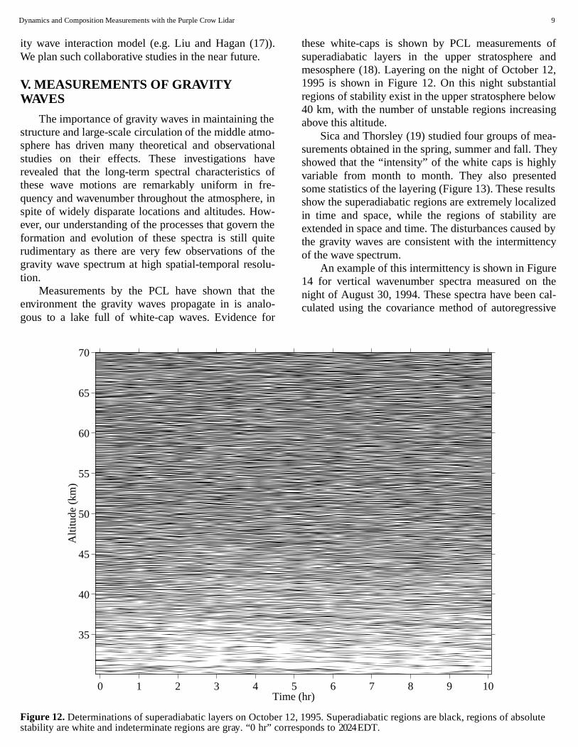
Measurements by the PCL have shown that environment the gravity waves propagate in is anagous to a lake full of white-cap waves. Evidence f

Figure 12. Determinations of superadiabatic layers on Octobstability are white and indeterminate regions are gray. “0 hr” co

Time

Alti

tude

(km

)

0 1 2 3 4 5

35

40

45

50

55

60

65

70

-alef

in-he

e-

e-

these white-caps is shown by PCL measurementssuperadiabatic layers in the upper stratosphere mesosphere (18). Layering on the night of October 1995 is shown in Figure 12. On this night substantregions of stability exist in the upper stratosphere bel40 km, with the number of unstable regions increasabove this altitude.

Sica and Thorsley (19) studied four groups of mesurements obtained in the spring, summer and fall. Tshowed that the “intensity” of the white caps is highvariable from month to month. They also presentsome statistics of the layering (Figure 13). These resshow the superadiabatic regions are extremely localiin time and space, while the regions of stability aextended in space and time. The disturbances causethe gravity waves are consistent with the intermittenof the wave spectrum.

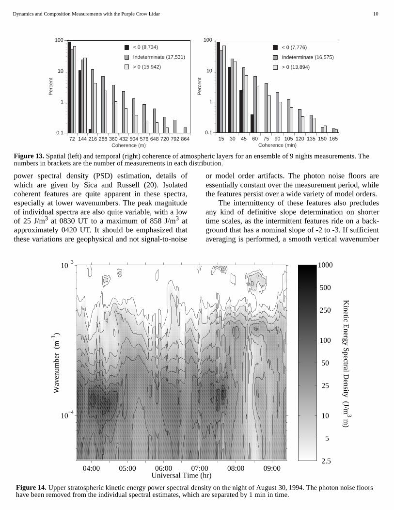
An example of this intermittency is shown in Figu14 for vertical wavenumber spectra measured on night of August 30, 1994. These spectra have been culated using the covariance method of autoregres

er 12, 1995. Superadiabatic regions are black, regions of absolute rresponds to 2024 EDT.

(hr)6 7 8 9 10


oedctdw

ais

rehilers.es

erck-ntber

Figure 13. Spatial (left) and temporal (right) coherence of atmospheric layers for an ensemble of 9 nights measurements. The numbers in brackets are the number of measurements in each distribution.

15 30 45 60 75 90 105 120 135 150 1650.1

1

10

100

Per

cent

Coherence (min)

< 0 (7,776)

Indeterminate (16,575)

> 0 (13,894)

72 144 216 288 360 432 504 576 648 720 792 8640.1

1

10

100

Per

cent

Coherence (m)

< 0 (8,734)

Indeterminate (17,531)

> 0 (15,942)

power spectral density (PSD) estimation, details which are given by Sica and Russell (20). Isolatcoherent features are quite apparent in these speespecially at lower wavenumbers. The peak magnituof individual spectra are also quite variable, with a loof 25 J/m3 at 0830 UT to a maximum of 858 J/m3 atapproximately 0420 UT. It should be emphasized ththese variations are geophysical and not signal-to-no

Figure 14. Upper stratospheric kinetic energy power spectrahave been removed from the individual spectral estimates,

04:00 05:00 06:00 07:

10−4

10−3

Universal Time

Wav

enum

ber

(m−

1 )

f

ra,e

te

or model order artifacts. The photon noise floors aessentially constant over the measurement period, wthe features persist over a wide variety of model orde

The intermittency of these features also precludany kind of definitive slope determination on shorttime scales, as the intermittent features ride on a baground that has a nominal slope of -2 to -3. If sufficieaveraging is performed, a smooth vertical wavenum

l density on the night of August 30, 1994. The photon noise floors which are separated by 1 min in time.

Kinetic E

nergy Spectral D

ensity (J/m 3 m)

2.5

5

10

25

50

100

250

500

1000

00 08:00 09:00 (hr)


dhe

thtlyviurm

fito

tino-selikesera

onti

ticbeitycu

wn-

yates

he

e

hegh

ityeddeforbyhe

spectrum with the expected -3 slope will be obtaineproviding a check on the signal-to-noise ratios of tmeasurements.

This averaging of high resolution spectra wiquasi-monochromatic features into an apparensmooth continuous spectrum suggests that the grawave spectrum may actually be composed of a mixtof quasi-monochromatic waves and a broad spectruSica and Russell (22) use Prony’s method (21) toexponentially damped sinusoids to the upper straspheric density perturbation data series. The resulfits are typically dominated by 3 or 4 quasi-monochrmatic features at lower wavenumbers. Sica and Rusalso show that classical statistical PSD estimators, the periodogram and correlogram, tend to blend thfeatures into a continuous power law due to their inhently poor spectral resolution. Parametric PSD estimtors are a much better choice for higher resolutistudies because they are much more adept at isolathe individual waves in the spectrum.

This dominance of only a few quasi-monochromafeatures in upper stratospheric vertical wavenumspectra may also help explain why Lindzen-type gravwave parametrizations appear to work in general cir

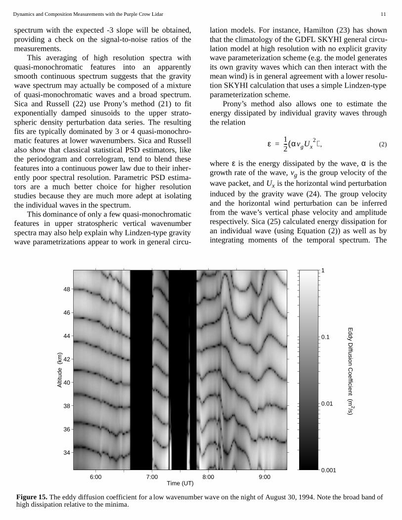
Figure 15. The eddy diffusion coefficient for a low wavenumbehigh dissipation relative to the minima.

Time (UT)

Alti

tude

(km

)

6:00 7:00 8

34

36

38

40

42

44

46

48

,

tye.

t-g

llee--

ng

r

-

lation models. For instance, Hamilton (23) has shothat the climatology of the GDFL SKYHI general circulation model at high resolution with no explicit gravitwave parameterization scheme (e.g. the model generits own gravity waves which can then interact with tmean wind) is in general agreement with a lower resolu-tion SKYHI calculation that uses a simple Lindzen-typparameterization scheme.

Prony’s method also allows one to estimate tenergy dissipated by individual gravity waves throuthe relation

, (2)

where ε is the energy dissipated by the wave, α is thegrowth rate of the wave, vg is the group velocity of thewave packet, and Ux is the horizontal wind perturbationinduced by the gravity wave (24). The group velocand the horizontal wind perturbation can be inferrfrom the wave’s vertical phase velocity and ampliturespectively. Sica (25) calculated energy dissipation an individual wave (using Equation (2)) as well as integrating moments of the temporal spectrum. T

ε 12--- αvgUx

2( )=

r wave on the night of August 30, 1994. Note the broad band of

Eddy D

iffusion Coefficient (m

2/s)

0.001

0.01

0.1

1

:00 9:00


eult a

s6

ere

ur- thte

-ionheut

otym

n-

lu-re.

rale of

-off.30,ea-

ea-ub-

p-ith0

re

s

resulting energy dissipations were similar, on the ordof 1 to 10 mW/kg in the upper stratosphere. The resing energy dissipations were then used to estimateeddy diffusion coefficient.

The eddy diffusion coefficient, D, can be inferredfrom

, (3)

where N2 is the angular buoyancy frequency, and β is aconstant. Most studies assume that β is independent oftime, with values in the range of 0.2 to 1.0 being mocommon. However, it has been shown by McIntyre (2that β is actually a function of the vertical wavenumbspectrum’s saturation. The parametric models employin these studies allow the saturation-dependent β to beestimated as a function of time, with the somewhat sprising result that β is 5 to 10 times smaller than typically assumed. It also suggests that the variations invertical wavenumber spectrum, and their associaeffects on β, may be the largest source of uncertainty inthe determination of the eddy diffusion coefficient.

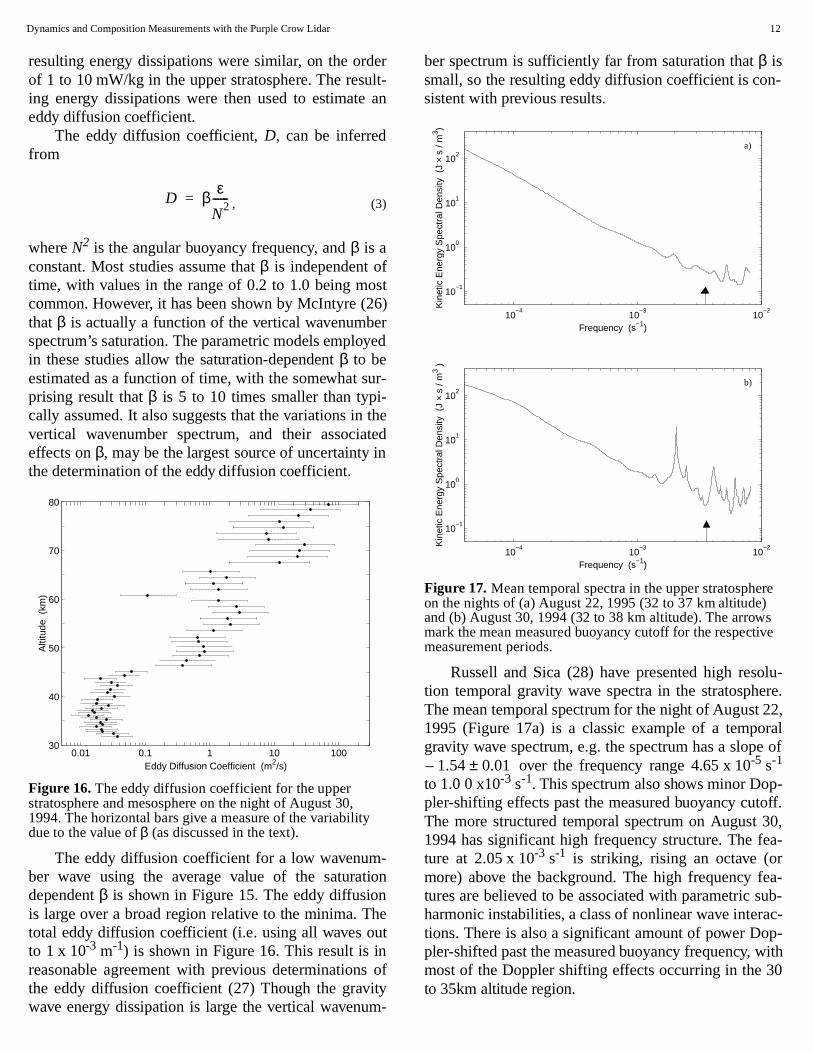
The eddy diffusion coefficient for a low wavenumber wave using the average value of the saturatdependent β is shown in Figure 15. The eddy diffusiois large over a broad region relative to the minima. Ttotal eddy diffusion coefficient (i.e. using all waves oto 1 x 10-3 m-1) is shown in Figure 16. This result is inreasonable agreement with previous determinationsthe eddy diffusion coefficient (27) Though the graviwave energy dissipation is large the vertical wavenu

Figure 16. The eddy diffusion coefficient for the upper stratosphere and mesosphere on the night of August 30, 1994. The horizontal bars give a measure of the variabilitydue to the value of β (as discussed in the text).

D β εN2------=

0.01 0.1 1 10 10030

40

50

60

70

80

Eddy Diffusion Coefficient (m2/s)

Alti

tude

(km

)

r-n

t)

d

-

ed

n

f

-

ber spectrum is sufficiently far from saturation that β issmall, so the resulting eddy diffusion coefficient is cosistent with previous results.

Russell and Sica (28) have presented high resotion temporal gravity wave spectra in the stratospheThe mean temporal spectrum for the night of August 22,1995 (Figure 17a) is a classic example of a tempogravity wave spectrum, e.g. the spectrum has a slop

over the frequency range 4.65 x 10-5 s-1

to 1.0 0 x10-3 s-1. This spectrum also shows minor Doppler-shifting effects past the measured buoyancy cutThe more structured temporal spectrum on August 1994 has significant high frequency structure. The fture at 2.05 x 10-3 s-1 is striking, rising an octave (ormore) above the background. The high frequency ftures are believed to be associated with parametric sharmonic instabilities, a class of nonlinear wave interac-tions. There is also a significant amount of power Dopler-shifted past the measured buoyancy frequency, wmost of the Doppler shifting effects occurring in the 3to 35km altitude region.

Figure 17. Mean temporal spectra in the upper stratospheon the nights of (a) August 22, 1995 (32 to 37 km altitude) and (b) August 30, 1994 (32 to 38 km altitude). The arrowmark the mean measured buoyancy cutoff for the respective measurement periods.

10−4

10−3

10−2

10−1

100

101

102

a)

Frequency (s−1)

Kin

etic

Ene

rgy

Spe

ctra

l Den

sity

(J

× s

/ m3 )

10−4

10−3

10−2

10−1

100

101

102

b)

Frequency (s−1)

Kin

etic

Ene

rgy

Spe

ctra

l Den

sity

(J

× s

/ m3 )

1.54– 0.01±


thersihesuofelom

oero

heno-in

nd

edos

cepare

rxyo

in a.isd

ple tongte

edortoo

isy, theve-

the,

a-ndh ashe).

tlywer

ix-

t 7

ios ofilere-file

pe-

ntheE-2

tudy no

The presence of these higher frequency featuresthe temporal spectra suggests that wave activity in stratosphere may be larger than that found in gencirculation models. These features also suggest that nificant amounts of energy may be dissipated in tmiddle upper stratosphere at certain times. This rehas important implications in the determination upper stratospheric eddy diffusion coefficients, as was the interpretation of the wave spectrum obtained frgeneral circulation models.

VI. TROPOSPHERIC AND LOWER STRATOSPHERIC WATER VAPOUR

Water vapour is perhaps the most important minconstituent, particularly in the troposphere. Watvapour absorbs radiation which helps drive the atmspheric circulations. Water vapour also modifies tradiative transfer of infrared absorption and can codense to form clouds. Improved measurements of tropspheric water vapour can lead to a better understandof cloud formation, convective storm development, athe hydrological cycle.

Water vapour mixing ratios are usually conservfor most atmospheric processes (evaporation and cdensation are the exceptions). Thus, it can used atracer of air parcels (29,30). When used as a trawater vapour measurements of sufficient temporal-stial bandwidth can be used in studies of stratosphetroposphere exchange.

Lower stratospheric water vapour also has impotant chemical considerations as a source for hydroradicals, which are important in the cleansing the atmsphere of many anthropogenic compounds, includchlorine and nitrogen species. Water vapour also hasimportant role in the chemistry of stratospheric ozone

Despite its importance, knowledge of the mean dtribution of water vapour, its seasonal variability, anthe processes that control it are limited. The PurCrow Raman-scatter Lidar (PCRL) is now configuredobtain routine measurements of water vapour mixiratio in the troposphere and lower stratosphere. Wavapour mixing ratios are obtained from the returnphotocount profiles. After appropriate processing (fbackground signal, count nonlinearity, etc.), the phocount profiles can be used to determine the water vapvolume mixing ratio, , since

. (4)

W z( )

W z( ) RN2

εστ z( )[ ]N2

εστ z( )[ ]H2O------------------------------

NH2Oz( )

NN2z( )--------------------⋅ ⋅=

inealg-

lt

l

r

-

-

g

n- ar,--

-l-gn

-

r

-ur

The ratio of the N2 density to that of dry air, , is

assumed constant with altitude. The term the product of the photomultiplier quantum efficiencthe vibrational Raman scattering cross section, andatmospheric transmission at the appropriate walengths for scattering from N2 and water vapour, 607.3nm and 660.3 nm respectively. These factors convertratio of the corrected photocounts,

into units of ppmv. Since the photocount profiles mesured by the PCRL are collected simultaneously athen used to determine a ratio, system variations suclaser power fluctuations which affect both profiles in tsame manner, cancel each other out (see Section II.2

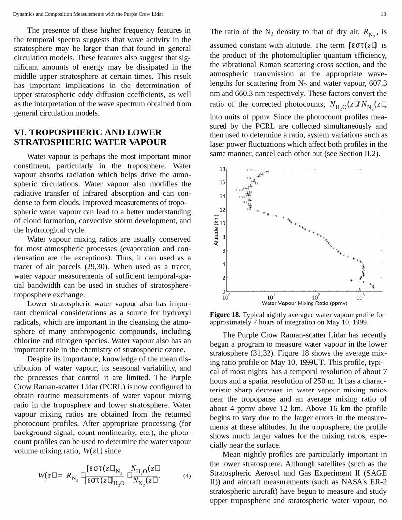
The Purple Crow Raman-scatter Lidar has recenbegun a program to measure water vapour in the lostratosphere (31,32). Figure 18 shows the average ming ratio profile on May 10, 1999 UT. This profile, typi-cal of most nights, has a temporal resolution of abouhours and a spatial resolution of 250 m. It has a charac-teristic sharp decrease in water vapour mixing ratnear the tropopause and an average mixing ratioabout 4 ppmv above 12 km. Above 16 km the profbegins to vary due to the larger errors in the measuments at these altitudes. In the troposphere, the proshows much larger values for the mixing ratios, escially near the surface.

Mean nightly profiles are particularly important ithe lower stratosphere. Although satellites (such as Stratospheric Aerosol and Gas Experiment II (SAGII)) and aircraft measurements (such as NASA's ERstratospheric aircraft) have begun to measure and supper tropospheric and stratospheric water vapour,

Figure 18. Typical nightly averaged water vapour profile forapproximately 7 hours of integration on May 10, 1999.

RN2

εστ z( )[ ]

NH2O z( ) NN2z( )⁄

100

101

102

103

0

2

4

6

8

10

12

14

16

18

Water Vapour Mixing Ratio (ppmv)

Alti

tude

(km

)


s deo

lat

0,km15s

br,of-ro dnte

eaurgoxC99

alneress re

io

owinge,veis

ageisdgethiser-

oda-e a

ity

ssesesure-tis-e ofr-

ere

er-oth

idarts ofnd

ra-ue

0,

long-term databases of water vapour measurementthese regions exist. The PCRL is the only mid-latituground-based system able to make routine water vapmeasurements in the lower stratosphere at middle tudes.

The mean value of the mixing ratio on May 11999 is between 3.5 to 4 ppmv between 12 and 15 with statistical errors of about 2% at 10 km, 12% at km and 17% at 18 km (Figure 19). The mixing ratiovalues are consistent with measurements obtainedballoon-borne frost-point hygrometers from BouldeColorado between 1981 and 1994 by Oltmans and Hmann (33). Another similarity to the Oltmans and Homann measurements is that the mixing ratio values dsharply just above the troposphere. This decrease isto the isothermal layer at the tropopause which prevesignificant vertical mixing of water vapour into thstratosphere.

Oltmans and Hofmann have also shown that a ssonal variation exists in stratospheric water vapoSpring mixing ratios are lower than summer mixinratios just above the tropopause, but converge to apprimately the same values at higher altitudes. The Pmeasurements in the late spring and summer of 1show a similar variation (Figure 19).

The PCRL averages only span two and a hmonths (versus the 14 years of Oltmans and Hofmanmeasurements). A larger database comprising sevyears is necessary to quantify any seasonal differenc

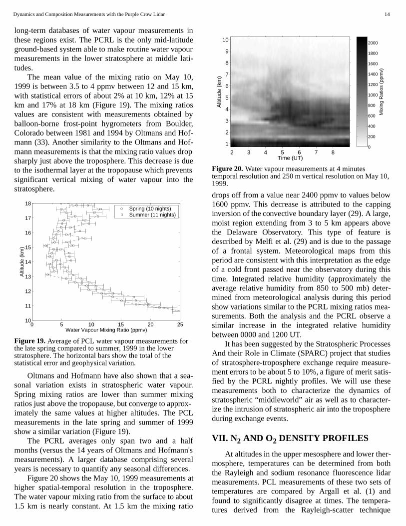
Figure 20 shows the May 10, 1999 measurementhigher spatial-temporal resolution in the tropospheThe water vapour mixing ratio from the surface to about1.5 km is nearly constant. At 1.5 km the mixing rat

Figure 19. Average of PCL water vapour measurements for the late spring compared to summer, 1999 in the lower stratosphere. The horizontal bars show the total of the statistical error and geophysical variation.

0 5 10 15 20 2510

11

12

13

14

15

16

17

18

Water Vapour Mixing Ratio (ppmv)

Alti

tude

(km

)

Spring (10 nights)Summer (11 nights)

in

uri-

,

y

f-

pues

-.

-L9

f'sal.

at.

drops off from a value near 2400 ppmv to values bel1600 ppmv. This decrease is attributed to the cappinversion of the convective boundary layer (29). A largmoist region extending from 3 to 5 km appears abothe Delaware Observatory. This type of feature described by Melfi et al. (29) and is due to the passof a frontal system. Meteorological maps from thperiod are consistent with this interpretation as the eof a cold front passed near the observatory during time. Integrated relative humidity (approximately thaverage relative humidity from 850 to 500 mb) detemined from meteorological analysis during this perishow variations similar to the PCRL mixing ratios mesurements. Both the analysis and the PCRL observsimilar increase in the integrated relative humidbetween 0000 and 1200 UT.

It has been suggested by the Stratospheric ProceAnd their Role in Climate (SPARC) project that studiof stratosphere-troposphere exchange require measment errors to be about 5 to 10%, a figure of merit safied by the PCRL nightly profiles. We will use thesmeasurements both to characterize the dynamicsstratospheric “middleworld” air as well as to characteize the intrusion of stratospheric air into the troposphduring exchange events.

VII. N 2 AND O2 DENSITY PROFILES

At altitudes in the upper mesosphere and lower thmosphere, temperatures can be determined from bthe Rayleigh and sodium resonance fluorescence lmeasurements. PCL measurements of these two setemperatures are compared by Argall et al. (1) afound to significantly disagree at times. The tempetures derived from the Rayleigh-scatter techniq

Figure 20. Water vapour measurements at 4 minutes temporal resolution and 250 m vertical resolution on May 11999.

Mix

ing

Rat

ios

(ppm

v)

0

200

400

600

800

1000

1200

1400

1600

1800

2000

Time (UT)

Alti

tude

(km

)

2 3 4 5 6 7 8

1

2

3

4

5

6

7

8

9

10


til

- o ijose

o b dio

he tr a

ckgmtil

eseaerormwme

s

ea-ec- to

4).weeatss

onwer

w-l-to-esend-

.s. Wegi-gi-

andent

.

. F.l.

s.

l.

p.

r-,

R.,.s.

.

7.

assume that the atmospheric constituent mixing raand cross section are constant with altitude and equatheir sea level values (3). However, the Na lidar temperature is a direct measure of the kinetic temperaturethe atmosphere (34-36). The disagreement foundArgall et al. suggests that the mixing ratio of the maatmospheric constituents is not always equal to its level value in the upper mesosphere and lower thermsphere. Neutral composition measurements maderocket borne mass spectrometers have also observedferences from the sea level values in this altitude reg(37-42).

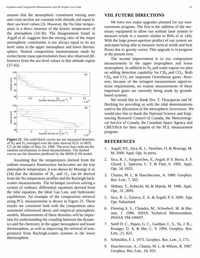
Assuming that the temperatures derived from tsodium resonance fluorescence backscatter are theatmospheric temperature, it was shown by Mwangi et(34) that the densities of and can be derivedfrom the Na temperature profiles and the Rayleigh bascatter measurements. The technique involves solvinsystem of ordinary differential equations derived frothe lidar equation, the Ideal Gas Law, and hydrostaequilibrium. An example of the composition retrievausing PCL measurements is shown in Figure 21. Thresults are consistent both with the composition msurements referenced above and empirical atmosphmodels. Measurements of these densities will be imptant for understanding the coupling between the dynaics and the chemistry in the upper mesosphere and lothermosphere, as well as improving the retrieval of teperatures from Rayleigh-scatter systems in the lowthermosphere.

Figure 21. The solid black curves are our measured densitieof N2 and O2 averaged over the time interval 0231 to 0835 UT on the night of May 24, 1998. The error bars indicate the random uncertainties in these measurements. The dashedcurves are the densities predicted by the MSIS-E-90 model.

0 0.5 1 1.5 2 2.5

x 1020

80

85

90

95

100

Number Density of N2 (m−3 )

Alti

tude

(km

)

(a)

0 2 4 6 8 10

x 1019

80

85

90

95

100

Number Density of O2 (m−3 )

Alti

tude

(km

)

(b)

N2 O2

oto

fnra-yif-n

uel.

- a

c

e-ic--er-r

VIII. FUTURE DIRECTIONS

We have two major upgrades planned for our msurements program. The first is the addition of the nessary equipment to allow our sodium laser systemmeasure winds in a manner similar to Bills el al. (4With the large power-aperture product of our system anticipate being able to measure vertical winds and hfluxes due to gravity waves. This upgrade is in progreat the present time.

The second improvement is to our compositimeasurements in the upper troposphere and lostratosphere. In addition to N2 and water vapour we planon adding detection capability for CH4 and CO2. BothCH4 and CO2 are important Greenhouse gases. Hoever, because of the stringent measurement signanoise requirements, no routine measurements of thimportant gases are currently being made by groubased systems.

We would like to thank Drs. T. Thayaparan and WHocking for providing us with the tidal determinationused in the discussion of the mesospheric inversionswould also like to thank the National Science and Enneering Research Council of Canada, the Meteorolocal Service of Canada, the Canadian Space AgencyCRESTech for their support of the PCL measuremprogram.

REFERENCES

1. Argall, P.S., Sica, R. J., Vassiliev, O. & Mwangi, MM. 2000. Appl. Opt. In press.

2. Sica, R. J., Sargoytchev, S., Argall, P. S. Borra, EGirard, L. Sparrow, C. T. & Flatt, S. 1995. AppOpt. 34, 6925.

3. Chanin, M. L. & Hauchecorne, A. 1980. GeophyRes. Lett., 7, 565.

4. Shibata, T., Kobuchi, M, & Maeda, M. 1986. AppOpt., 31, 2095.

5. Sica, R. J., Zylawy, Z. A. & Argall, P. S. 2000. ApOpt. Submitted.

6. Fleming S. S., Chandra, M., Schoeberl, M. & Banett, J. 1988. NASA Technical Memorandum#NASA TM-100697.

7. Senft D. C., Papen, G. C., Gardner, C. S., Yu, J. Krueger, D. A. & She, C. Y. 1994. Geophys. ReLett., 21, 821.

8. Schmidlin, F. J. 1975. Geophys. Res. Lett., 3, 173

9. Hauchecorne, A., Chanin, M. L. & Wilson, R. 198Geophys. Res. Lett., 14, 933.


ys

.

S.

e

-.

Ab-

.

s.

s

.er,

6

.

es

-log,

7.

43

es

.

.

ity

p.

4,

S.

r.

.

.

.,e-

ch,

8.

-

1,

n,

J.

pt.

10. Leblanc, T. & Hauchecorne, A. J. 1997. J. GeophRes. 102, 19,471.

11. Whiteway, J. A., Carswell, A. I. & Ward, W. E1995. Geophys. Res. Lett., 22, 1201.

12. Dao, P. D., Farley, R., Tao, X. & Gardner, C. 1995. Geophys. Res. Lett., 20, 2825.

13. States, R. J. & Gardner, C. S. 1998. Geophys. RLett., 25, 1483.

14. Meriwether, J. W., Gao, X., Wickwar, V. B., Wilkerson, T. Beissner, K. Collins, S. & Hagan, M. E1998. Geophys. Res. Lett., 25, 1479.

15. Sica, R. J., Thayaparan, T., Argall, P. S. Russell,T. & Hocking, W. K. 2000. J. Geophys. Res., sumitted.

16. Thayaparan, T., Hocking, W. K. & MacDougall, J1995. Radio Sci. 30, 1293.

17. Liu, Han-Li & Hagan, M. 1998. Geophys. ReLett., 25, 2941.

18. Sica, R. J. & Thorsley, M. D. 1996. Geophys. ReLett., 23, 2797.

19. Sica, R. J. & Thorsley, M. D. 1997. In: Hamilton, K(Editor), Gravity Wave Processes. Their Parametization in Global Climate Models, page 27Springer-Verlag, Berlin.

20. Sica, R. J. & Russell, A. T. 1999. J. Atmos. Sci., 51308.

21. Marple, S. L. 1987. Digital Spectral AnalysisChapter 11, Prentice Hall, Englewood Cliffs, NJ.

22. Sica, R. J. & Russell, A. T. 1999. Geophys. RLett. 26, 3617.

23. Hamilton, K. 1997. In: Hamilton, K. (Editor), Gravity Wave Processes. Their Parameterization in Gbal Climate Models, page 337, Springer-VerlaBerlin.

24. Hines, C. O. 1965. J. Geophys. Res. 70, 177.

25. Sica, R. J. 1999. J. Atmos. Sci., 56, 1330.

26. McIntyre, M. E 1989. J. Geophys. Res., 89, 1461

27. Hocking, W. K. 1991. J. Geomagn. Geoelectr. (Suppl.), 621.

28. Russell, A. T. & Sica, R. J. 2000. J. Geophys. RSubmitted.

29. Melfi, S. H., Whiteman, D. N. & Ferrare, R. A1989. J. App. Meteor. 28, PAGE.

.

s.

.

.

-

,

.

-

.

30. Whiteman, D. N., Ferrare, R. A. & Melfi, S. H1992. App. Opt. 31, PAGE.

31. Bryant, C. R. 1999. M. Sc. Thesis, The Universof Western Ontario.

32. Bryant, C. R., Argall, P. S. & Sica, R. J. 2000. ApOpt. Submitted.

33. Oltmans, S. J. & Hofmann, D. J. 1995. Nature. 37146.

34. Gibson, A., Thomas, L. & Bhattachacharyya, 1979. Nature, 281, 131.

35. Fricke, K. H., & von Zahn, U. 1985. J. Atmos. TerPhys., 47, 49.

36. She, C. Y., Yu, J.R. Latifi, H & Bills, R. E. 1992Appl. Opt., 31, 2095.

37. Philbrick, C. R., Faucher, G. A. & Trzcinsky, E1973. Space Research, 13, 255.

38. Philbrick, C. R., Golomb, D., Zimmerman, S. PKeneshea, T. J., MacLeod, M., Good, R. E., Dandkar, B. S. & Reinisch, B. W. 1974. Space Resear14, 89.

39. Philbrick, C. R, Faucher, G. & Bench, P. 197Space Research, 18, 139.

40. Trinks, H., Offermann, D., von Zahn, U. & Steinhauer, C. 1978. J. Geophys. Res., 83, 2169.

41. Krankowsky, D., Arnold, F., Friedrich, V. H. &Offermann, D. 1979. J. Atmos. Terr. Phys., 41085.

42. Offermann D., Friedrich, V., Ross, P. & von. ZahU. 1981. Planet Space Sci., 29, 747.

43. Mwangi, M. M., Sica, R. J. & Argall, P. S. 2000. Geophys. Res. Submitted.

44. Bills, R. E., Gardner, C. S. & She, C. Y. 1991. OEng., 30, 13.

dynamics and composition measurements with the...

Documents