dynamics and control of tethered satellite formations in
TRANSCRIPT

Dynamics and Control of Tethered Satellite Formations in
Low-Earth Orbits
PhD Thesis
Manrico Fedi Casas
Universitat Politecnica de Catalunya
2015


To Flavia


Contents
1 Introduction 3
1.1 Objectives of the study . . . . . . . . . . . . . . . . . . . . . . . . . . . . . 3
1.2 Tethers in space and flight formation . . . . . . . . . . . . . . . . . . . . . . 3
1.3 State of the Art . . . . . . . . . . . . . . . . . . . . . . . . . . . . . . . . . . 5
1.3.1 Space Tether Applications . . . . . . . . . . . . . . . . . . . . . . . . 5
1.3.2 Tether Simulation Analysis . . . . . . . . . . . . . . . . . . . . . . . 8
1.3.3 Tether Control Approach . . . . . . . . . . . . . . . . . . . . . . . . 9
1.4 Space Tether Missions . . . . . . . . . . . . . . . . . . . . . . . . . . . . . . 9
1.4.1 TSS mission . . . . . . . . . . . . . . . . . . . . . . . . . . . . . . . . 10
1.4.2 SEDS-1 and SEDS-2 missions . . . . . . . . . . . . . . . . . . . . . . 11
1.4.3 TiPS mission . . . . . . . . . . . . . . . . . . . . . . . . . . . . . . . 13
1.4.4 YES2 mission . . . . . . . . . . . . . . . . . . . . . . . . . . . . . . . 14
1.4.5 SPECS mission . . . . . . . . . . . . . . . . . . . . . . . . . . . . . . 14
1.5 Thesis Outline . . . . . . . . . . . . . . . . . . . . . . . . . . . . . . . . . . 14
1.5.1 Objectives of the study . . . . . . . . . . . . . . . . . . . . . . . . . 14
1.5.2 Thesis structure . . . . . . . . . . . . . . . . . . . . . . . . . . . . . 15
1.5.3 Contributions . . . . . . . . . . . . . . . . . . . . . . . . . . . . . . . 17
2 Flight Dynamics of Tethered Formations 18
2.1 Review of Orbital Mechanics . . . . . . . . . . . . . . . . . . . . . . . . . . 18
2.2 Dynamics of Relative Motion . . . . . . . . . . . . . . . . . . . . . . . . . . 22
2.2.1 Equations of motion relative to a reference orbit . . . . . . . . . . . 22
2.2.2 Relative equations of Motion based on Orbit Elements . . . . . . . . 30
2.2.3 Comparison of orbital models . . . . . . . . . . . . . . . . . . . . . . 31
2.3 Effects of Orbit Perturbations . . . . . . . . . . . . . . . . . . . . . . . . . . 32
2.3.1 Perturbations in Equations of Motion . . . . . . . . . . . . . . . . . 33
2.3.2 Implementation of the J2 Perturbation . . . . . . . . . . . . . . . . . 35
i

2.4 Tether Models . . . . . . . . . . . . . . . . . . . . . . . . . . . . . . . . . . 39
2.4.1 Elasticity Model . . . . . . . . . . . . . . . . . . . . . . . . . . . . . 40
2.4.2 Effects of tether mass . . . . . . . . . . . . . . . . . . . . . . . . . . 41
2.4.3 Tether Deployment and Retrieval . . . . . . . . . . . . . . . . . . . . 46
2.4.4 Dynamics of a tether in orbit . . . . . . . . . . . . . . . . . . . . . . 47
2.5 Cluster Architectures . . . . . . . . . . . . . . . . . . . . . . . . . . . . . . . 55
2.5.1 Planar Formations . . . . . . . . . . . . . . . . . . . . . . . . . . . . 55
2.5.2 Three Dimensional Formations . . . . . . . . . . . . . . . . . . . . . 56
2.6 Formation Spin Stabilization . . . . . . . . . . . . . . . . . . . . . . . . . . 56
2.6.1 Double Pyramid Global Formation Behavior . . . . . . . . . . . . . 59
2.7 Agent Control . . . . . . . . . . . . . . . . . . . . . . . . . . . . . . . . . . . 60
3 Refined dynamical analysis of multi-tethered satellite formations 63
3.1 Tether Model . . . . . . . . . . . . . . . . . . . . . . . . . . . . . . . . . . . 63
3.2 Initial conditions . . . . . . . . . . . . . . . . . . . . . . . . . . . . . . . . . 64
3.3 Open loop stability analysis . . . . . . . . . . . . . . . . . . . . . . . . . . . 66
3.3.1 In-plane formations . . . . . . . . . . . . . . . . . . . . . . . . . . . 69
3.3.2 Earth-facing formations . . . . . . . . . . . . . . . . . . . . . . . . . 75
3.4 Circular formations . . . . . . . . . . . . . . . . . . . . . . . . . . . . . . . . 84
3.4.1 Closed Hub-And-Spoke in-plane formation . . . . . . . . . . . . . . . 84
3.4.2 Earth-facing formations . . . . . . . . . . . . . . . . . . . . . . . . . 88
3.5 Major findings for tethered formation dynamics . . . . . . . . . . . . . . . . 89
4 Multi-tethered formation dynamics for non-ideal operating conditions 92
4.1 Effects of eccentricity of the reference orbit on Multi–Tethered Satellite
Formations . . . . . . . . . . . . . . . . . . . . . . . . . . . . . . . . . . . . 92
4.1.1 Initial conditions for deputies and beads . . . . . . . . . . . . . . . . 94
4.1.2 Formation stability . . . . . . . . . . . . . . . . . . . . . . . . . . . . 97
4.1.3 Behavior of the parent body . . . . . . . . . . . . . . . . . . . . . . . 112
4.1.4 Effects of eccentricity of the reference orbit . . . . . . . . . . . . . . 114
4.2 Effects of J2 perturbation on tethered formations . . . . . . . . . . . . . . . 116
4.2.1 Initial conditions for deputies and beads . . . . . . . . . . . . . . . . 116
4.2.2 Proposed approach . . . . . . . . . . . . . . . . . . . . . . . . . . . . 117
4.2.3 Open–loop dynamics of tethered formation . . . . . . . . . . . . . . 118
4.2.4 Effect of the J2 perturbation on the parent body . . . . . . . . . . . 122
4.2.5 Effects of J2 perturbation on formation behavior . . . . . . . . . . . 124
ii

5 Tethered Formation Control 129
5.1 Formation Flying Control . . . . . . . . . . . . . . . . . . . . . . . . . . . . 129
5.2 Tethered Formation Flying Control . . . . . . . . . . . . . . . . . . . . . . . 130
5.3 Virtual Structure Control Approach . . . . . . . . . . . . . . . . . . . . . . 131
5.3.1 Centralized Virtual Structure Control Approach . . . . . . . . . . . 131
5.3.2 Decentralized Virtual Structure Control Approach . . . . . . . . . . 133
5.4 VSC model for a spinning Double-Pyramid formation orbiting a central body135
5.5 Fine positioning control . . . . . . . . . . . . . . . . . . . . . . . . . . . . . 139
5.5.1 Thruster Control Model . . . . . . . . . . . . . . . . . . . . . . . . . 139
5.5.2 Agent dynamics . . . . . . . . . . . . . . . . . . . . . . . . . . . . . 140
5.5.3 Control Approaches . . . . . . . . . . . . . . . . . . . . . . . . . . . 141
5.5.4 Sliding mode control . . . . . . . . . . . . . . . . . . . . . . . . . . . 143
5.6 Reeling and tether tension control . . . . . . . . . . . . . . . . . . . . . . . 147
5.7 Vibration control . . . . . . . . . . . . . . . . . . . . . . . . . . . . . . . . . 148
5.7.1 Longitudinal oscillations . . . . . . . . . . . . . . . . . . . . . . . . . 148
5.7.2 Transversal oscillations . . . . . . . . . . . . . . . . . . . . . . . . . 148
5.8 Control Results . . . . . . . . . . . . . . . . . . . . . . . . . . . . . . . . . . 149
5.9 VSC major findings . . . . . . . . . . . . . . . . . . . . . . . . . . . . . . . 154
6 Conclusions 156
Nomenclature 160
Acronyms 165
Bibliography 166
iii


Abstract
The thesis is focused on the study of dynamics and control of a multi–tethered satellite
formation, where a multi–tethered formation is made up with several satellites (agents)
connected by means of cables (tethers).
The interest in tethered formations emerged at the turn of the millennium. The con-
cept of tethered formation would benefit from the availability of a multi–agent system with
unique properties: the distribution of the payload over several elements of the formation
provides unprecedented mission capabilities, especially in terms of mission flexibility and
resilience to failures, while the use of tethers for stabilization and control purposes (and
possibly for communication between agents as well) would allow to manoeuvre and recon-
figure the formation simply by acting on tether length and tension in order to vary agents’
relative position. Mission effectiveness would thus be maximized at a very modest price
in terms of energy consumption, as far as no thrust is required for a manoeuvre requiring
the variation of tethers length only. Several scientific missions has been envisaged that
could benefit from this novel concept, especially in the field of interferometry.


Thesis Information
Thesis Title:
Dynamics and Control of Tethered Satellite Formations in Low-Earth Orbits
Thesis committee information
Thesis DirectorProfessor Giulio AvanziniUniversita del [email protected]
UPC TutorProfessor Josep Joaquim Masdemont SolerUniversitat Politecnica de [email protected]
Committee PresidentProfessor Gerard Gomez Muntane.Universitat de [email protected]
Committee SecretaryProfessor Ramon Costa CastelloUniversitat Politecnica de [email protected]
Committee VocalProfessor Camilla ColomboPolitecnico di [email protected]
Ph.D. CandidateManrico Fedi [email protected]
1


Acknowledgements
Thanks Montse for your constant love and support day after day. You always find the
right words for motivation. Thank you also for your patience for so many evenings and
weekends spent home because of my studies.
The values my parents taught me since I was a kid have brought me here. The eagerness
to pursue new challenges is something I owe them. I want to thank my parents Dolors
and Xavier, for their love and for the education they gave me.
Many thanks Giulio for your outstanding scientific guidance during my Ph.D. studies. Liv-
ing on different countries has not been a problem to perform this work. Your availability,
no matter the time of the day, or the day of the week, even during your own holidays, has
always been superb.
I would like to thank professors J.J. Masdemont Soler, D. Crespo Artiaga and R. Costa
Castello for their good advice, both technical and administrative received during my Ph.D.
studies.
I want to thank Pete Balsells for giving me the opportunity to perform graduate studies
at University of California through the Balsells - Generalitat de Catalunya fellowship pro-
gram. That opportunity was a crucial stepping stone in my career.
2


Chapter 1
Introduction
1.1 Objectives of the study
This thesis is focused on the study of dynamics and control of a multi-tethered satellite
formation, where a multi-tethered formation is made up with several satellites (agents)
connected by means of cables (tethers).
The goal of the first part of the study is to evaluate the effect of tether mass on multi-
tethered clusters. Due to the complexity of the formations analyzed, the stability of the
formation is assessed through a numerical simulation. The behavior is evaluated in the
ideal case of circular orbits, but also in non-ideal cases such as that of elliptical reference
orbit or perturbed motion.
The second part of the study is focused on deriving a control law for position and
attitude control of a multi-tethered cluster. The control problem is decomposed in two
levels: A first level to perform position and attitude coarse control of the formation as a
whole, and a second level to achieve accurate position and control of each agent of the
cluster. This approach benefits from the fact that tethers provide rigidity similar to that
of a rigid body, and therefore the cluster exhibits a behavior comparable to that of an
orbiting rigid body.
1.2 Tethers in space and flight formation
Tethers are cables that define a physical link between two or more satellites in order to
maintain a predefined configuration in space. As shown in [1], the potential applications
3

1 – Introduction
of deploying tether systems in space are multiple. The dynamics of tethers under the pres-
ence of gravity-gradient, drag and electrodynamic forces, the tether viscoelastic behavior,
the momentum transfer capabilities of taut tethers, and other features offer a wide range
of possibilities that can be useful for different space missions. A summary of space tether
applications and missions is presented in Section 1.4.
The concept of Satellite Formation Flying (SFF) consists of a cluster composed by
several satellites cooperating together. The purpose of this cooperation is to perform
missions, or achieve a degree of performance not achievable by a single satellite. The
characteristics of each mission will introduce requirements regarding the relative position
of each satellite and synchronized motion between them. Clearly, the use of tethers as
a link among formation constituents can be used to mechanically restrain their relative
motion thus providing a constraint for formation keeping purposes.
The concept of Tethered Formation Flying (TFF) benefits from the availability of a
multi-agent system with unique properties: the distribution of the payload over several
elements of the formation provides unprecedented mission capabilities, especially in terms
of mission flexibility and resilience to failures, while the use of tethers for stabilization and
control purposes (and possibly for communication between agents as well) would allow to
manoeuvre and reconfigure the formation simply by acting on tether length and tension
in order to vary agents’ relative position. Mission effectiveness would thus be maximized
at a very modest price in terms of energy consumption, as far as no thrust is required for
a manoeuvre requiring the variation of tethers length only. Several scientific missions has
been envisaged that could benefit from this novel concept, especially in the field of inter-
ferometry. Some of the TFF applications require high precision formation flying capability.
The purpose to study the effect of massive tethers is motivated by the relatively high
mass of tethers compared to that of a typical small satellite. The length of tethers belong-
ing to large formations, combined with the density of suitable tether materials, suggest
that the effect of the tether mass on the overall dynamics may not be negligible. Dou-
ble or triple strand tethers may increase further the effect of the mass on cluster dynamics.
The definition of a suitable tether physical model is fundamental. The model must
be rich enough to take into account the effect of the mass and vibration modes, but at
the same time its computational cost must be reasonable. The latter feature may be not
4

1 – Introduction
a concern for modeling single tethers in the space, but it is an issue for complex multi-
tethered structures with several links and equation couplings.
Multi-agent tethered formations are presented as a type of satellite flight formations.
Controlling the relative position of the agents is essential in many mission scenarios. For
this purpose, it is needed to be able to define accurately an arbitrary relative position
and attitude of the members of the cluster. The inclusion of the mass of the tethers in
the model complicates the control problem. On the massless case, under the assumption
that every agent has full control capability, the tether tension is easy to predict. On the
other hand, for the massive case, the force exerted by tethers on the deputies is not easy
to model due to the effect of external forces (mainly the gravity force, but also other
perturbations) on the mass of the tether. Therefore, the changes in tether tension due to
the effect on external forces on tether mass act as a disturbance.
1.3 State of the Art
1.3.1 Space Tether Applications
References [1] and [2] provide a rich and interesting summary of some of the potential ap-
plications of space tethers. References [3], [4], [5] and [6] provide an overview of the state
of the art of tether research. Most of tether space missions rely on one of the following
two fundamental characteristics (or a combination of both): use of tethers with the pur-
pose of momentum exchange, and use of tethers made of materials having electrodynamic
properties. The former application uses tethers essentially to transmit forces and/or to
distribute momentum to the members of the cluster. The latter takes into account the
forces generated in conductive tethers due to Ampere currents related to the Earth’s mag-
netic field, as explained in [7].
Among many others, some of the most significant applications are listed below.
• Comet rendez-vous and sample retrieval. The goal of the mission consist
in obtaining a sample of a comet. The capsule containing the sample would be
retrieved with a tether. This approach requires a penetrator harpoon containing an
inner sample capsule container. The penetrator is released, hits the comet, and then
the capsule containing the sample is retrieved with a tether attached to the mother
spacecraft [2].
5

1 – Introduction
• Spacecraft boosting through electrodynamic tether. This mission benefits
from the fact that Ampere forces along the velocity vector exert a force on the
spacecraft. In Ref. [2], Levin considers the mission setup that was intended to
extend the life of the Russian Mir space station on orbit. The dynamics involved take
into account vehicle attitude dynamics, electrodynamic control, resonant motions,
transverse oscillations, torque produced by the Ampere forces and variations on
the geomagnetic field. It is shown that the mass-to-current ratio increases with
instability. Based on the properties of electrodynamic tethers, Levin proposes the
creation of an electrodynamic sail, made of a grid of electrodynamic tethers.
• Object de-orbiting. The drag induced by electrodynamic forces can also be used
to remove objects from orbit. At the end of the life, a satellite may deploy a tether
that generates sufficient drag in order to de-orbit the satellite towards atmosphere
in a controlled way. Similarly, some research was performed to investigate the use of
tethers with the purpose of capturing orbiting debris through harpoon or throw-nets
[8].
• Momentum exchange electrodynamic reboost system. In this case, the pay-
load is captured by an end body that rotates at one of the ends of the spinning
tether system. This tether works as a skyhook, that releases the payload after half
a turn, providing it an additional delta-V that could be on the order of 2 km/s as
discussed in [2].
• Tether space elevator. The purpose of the tether is to provide a means for a
platform to lift payloads into orbit. The elevator (or climber, as called in some
references) should have a mean to climb along the tether. The end of the tether
should be connected to a ballast mass which acts as a counterweight. The center of
mass of the combined system should be above the geostationary orbit, in such a way
that the ballast would ”pull” the tether anchored to the Earth surface as described
in [9].
• Lunar transportation system. By using an Earth-Moon space elevator connected
through a transfer orbit it should be possible to transport material between Earth
and Moon. An additional vehicle or means of transportation would still be necessary
to lift material from the lunar surface up to the tether transportation system. This
case is analyzed in detail in reference [2]. The same reference also proposes an
alternative interplanetary tether transportation system between Martian low orbit,
up to escape orbit, by using tethers attached to the orbit of the moons of Mars.
6

1 – Introduction
• Atmospheric probe. The deployment of a tether from an orbiting spacecraft could
be used also with the purpose of a multi-probe for atmospheric studies. A probe
released from an orbiting vehicle could be used to acquire relevant measurements at
different atmosphere altitudes.
• Tethered space observatory. An observation platform can be created by defining
a mosaic of several satellites connected through tethers. The measurements of these
satellites could be combined in order to achieve high precision interferometry. This
could be comparable to using a telescope with a very large aperture that could be
used for different kinds of missions, including radio interferometry (as presented in
[10], [11] and [12]). Other applications could be multipoint measurement applica-
tions, or gravity measurement laboratories (as mentioned in [13]).
As stated before, this thesis focuses on the study of multi-body tethered formations
described in the last item of the above list. These formations consist of multi-body tethers
performing a coordinated movement.
The main advantages of using tethers for satellite flight formation are:
• Reduction of fuel consumption of agents. The natural stabilization of the
structure reduces the fuel consumption on devices using actuators to perform position
corrections. This is an advantage with respect to free flight formation formations.
Considerable fuel consumption limits the operative life of the system.
• Less actuators needed. The fact that tethers provide a natural way to prescribe
the position of certain constituents, and the wise use of gravitational and/or centrifu-
gal forces, may remove the need to use any actuator to perform position corrections.
Less actuators means cheaper satellites, less complexity, more reliability, and less
weight.
• Rigid body behavior. Under some conditions a tethered cluster behaves like a
rigid body. Therefore the equilibrium properties of orbiting rigid bodies are appli-
cable to tethered formations.
• Potential reduction in computational load. In a free flight formation, each
device shall perform its GNC calculations in order to assess the position at every
time. In this case it won’t be even necessary that certain orbiting bodies have a
CPU with GNC algorithm.
7

1 – Introduction
• Use of tethers for communications. For these cases when agents need to perform
a synchronized control, it is needed to establish a communication link between them.
Tethers can be used as a physical communication layer.
On the other hand, potential problems of tethered formation are:
• Lack of reconfiguration flexibility. Tethers impose reduced flexibility in terms
of formation reconfiguration. Physical links between the orbiting bodies constraint
the movements, as opposite to the non-tethered case where there is no limit to any
reconfiguration.
• Potential single point of failure. In case of failure of one of the constituents of
the formation or one of the tethers, it would not be possible to replace it. If the
system does not provide redundant components, the whole mission will be lost.
• Build complexity. Tethered formations require more complex mechanical con-
struction, as tethers need to link orbiting bodies. In systems with variable length
tethers, a reeling mechanism will have to be installed on one or several deputies.
• Complex deployment. The complete structure must be launched with tethers
already connecting orbiting bodies. Deployment can be complicated specially in
these missions where the constellation doesn’t have a variable tether mechanism
able to extend or retract tethers dynamically in orbit.
• Effect of tether mass As shown in this thesis, the effect of the mass of tethers is
not negligible. This acts as a perturbation to the position of the agents.
• Sensitivity to space debris. In some cases, space debris may hit and break
tethers, with the risk of endangering the whole mission.
1.3.2 Tether Simulation Analysis
Reference [13] provides the starting point for the analysis of the effect of tether mass. This
paper develops several analytical models for specific tethered formation configurations and
orientations. Based on analytical models, it performs a numerical analysis of the stability
of the studied formations through the results of simulations for the different formation
configurations studied. The model used in the cited paper does not take into account
tether mass. The work performed in this thesis defines equivalent massive formations
using the lumped mass model [14], [15] with the purpose of comparing the behavior of
8

1 – Introduction
massive and massless formations.
Paper [16] defines a model taking into account the effect of the J2 perturbation due
to the Earths oblateness. The advantage of this model is that is formulated in the LVLH
(Local Vertical Local Horizontal) reference frame, as it is the case of the HCW equations.
This model is used to evaluate the behavior of some of the tethered formations studied in
Ref. [13].
The model that incorporates eccentric orbits is presented in Ref. [17]. This paper
presents a model for elliptical orbits using true anomaly as independent variable that is
formulated also in the LVLH reference frame.
1.3.3 Tether Control Approach
The potential suitability of a double pyramid structure for an Earth-oriented cluster is
examined in papers [18] and [15]. The rigidity provided by the tethers provides a behavior
similar to that of a rigid body in orbit.
Reference [19] provides the basis for the development of a control law based on the
virtual structure principle. This paper defines an approach that allows taking advantage
of the rigidity of a tethered structure and the similarity of the behavior of the cluster with
that of rigid body. Several other papers [20], [21] and [22] by the same authors provide
different variations of the same control law.
For the precision control approach, Refs. [23] and [24] are taken into account. Both
papers are valid for the development of a control law for a second order system involving
a system of coupled equations.
1.4 Space Tether Missions
The first missions conducted with tethered systems had the purpose of assessing the pos-
sibility of deploying tethers over long distances, and to determine the potential stability
issues associated to them. Figure 1.1 shows a summary of past and future tethered mis-
sions organized by NASA. Table 1.1 lists the most relevant missions of Tethered Satellite
Systems (TSS) in LEO based on the information provided in Refs. [7], [25] and [26]. A set
of references providing details for each mission is found in [26].
9

1 – Introduction
Table 1.1: Flown tether missions in LEO
Name Year Organization Tether Length
Gemini XI 1966 NASA 30 m
Gemini XII 1967 NASA 30 m
TSS-1 1992 ASI/NASA 260 m
SEDS-1 1993 NASA 20 km
PMG 1993 NASA 500 m
SEDS-2 1994 NASA 20 km
Oedipus-C 1995 CRC/CSA/NASA/NRC 1 km
TSS-1R 1996 ASI/NASA 19.6 km
TiPS 1996 NRL/NRO 4 km
ATEx 1999 NRL/NRO 6 km
MAST 2007 NASA/Stanford/TUI 1 km
YES2 2007 ESA 30 km
STARS 2009 Kagawa University 5 m
T-REX 2010 ISAS/JAXA 300 m
TEPCE 2013 NRL/NRO 30 km
The first use of tethers in a space mission took place in 1966 during the Gemini XI
mission. The purpose of this mission was to perform a rendezvous between the Gemini
capsule and the Agena vehicle which consisted of a docking platform plus a power unit.
One of the secondary goals of the mission was to study the stability of the two spacecraft
connected through a 30 m tether. The success of this mission assessed the viability of
the use of tethers in space missions. Figure 1.1 provides a summary of some of the most
significant space missions conducted by NASA.
1.4.1 TSS mission
After the success of the Gemini mission, the TSS-1 (Tethered Satellite System) was the
first mission to test the possibilities of tether deployment in space [27]. The purpose of
this mission launched on 1992, was to provide the capability of deploying a satellite on
a long, gravity-gradient stabilized tether from the Space Shuttle. The (TSS) consisted
of three elements: a satellite (Spacelab pallet), an electrodynamic tether, and a tether
deployment/retrieval mechanism attached to the Space Shuttle (Fig. 1.2). The objectives
of the TSS-1 mission were:
10

1 – Introduction
Figure 1.1: Summary of missions with participation of tethered systems (Credit:NASA)
• To test the dynamics acting on a variable length tether.
• To determine and understand the electromagnetic interaction between the tether,
satellite, orbiter system and space plasma.
• To find potential future tether applications on the Shuttle and Space Station.
The TSS-1 released a satellite while remaining attached to a reel in the Shuttle payload
bay. Originally, it was intended to be deployed 20 km above the Shuttle, but due to a
malfunction in the reeling system it was deployed only to 268 m. However, this was enough
to proof that gravity-gradient stabilized tethers was a valid concept, and the feasibility to
deploy satellites to long distances.
1.4.2 SEDS-1 and SEDS-2 missions
The purpose of the Small Expendable Deployment System (SEDS) project was to test the
deployment of a 20 km satellite [1], [28], [29], [30].
11

1 – Introduction
The SEDS-1 mission demonstrated the capability of deorbiting a 25 kg payload from
LEO. The mission objectives were to demonstrate that it was possible to deploy a payload
at the end of a 20 km-long tether and to study its reentry after the tether was snapped.
The orbit chosen had an inclination of 34 degrees, a perigee altitude of 190 km and an
apogee altitude of 720 km.
The second mission SEDS-2, intended to demonstrate the use of a feedback closed
loop control law with the purpose of tracking a predetermined trajectory. The main goal
of the mission was the deployment of a payload along the local vertical. The mission
was intended also to assess the long term evolution of a tethered system. The orbit was
circular with an altitude of about 350 km. The SEDS-2 tether was presumably snapped
by a micrometeroid or space debris after five days of the mission.
Figure 1.2: TSS deployment system, tether, and satellite
12

1 – Introduction
1.4.3 TiPS mission
The purpose of the Tether Physics and Survivability (TiPS) mission [31], [32], was to study
the long-term behavior and longevity of tethers in space. This mission was motivated
by several tether failures in previous missions. Mission TSS-1 was aborted due to a
malfunction in the deployment mechanism, the tether of the SEDS-2 mission was cut off
by a micrometeorite, and the TSS-1R tether was cut off during deployment. After these
results it was needed to assess better the viability of a deployed tether in a long term
mission.
Figure 1.3: TiPS tether deployed as seen from observatory mesurements (Credit:NASA)
The formation consisted of two bodies (Ralph and Norton) connected by a tether 2 mm
diameter. Body Ralph (closest to the Earth) contained the electronics and the actuation
system, whereas Norton was a passive satellite. Figure 1.3 shows an image of the tether
system as observed from an optical station on ground. The only active mechanism of the
mechanism was the deployment device. The formation survived for more than 27 months.
Reference [33] provides a summary of the results, showing the evolution of the libration
amplitude and libration rate of the formation.
13

1 – Introduction
1.4.4 YES2 mission
The YES2 mission aimed at proving the viability of a tether deployment system plus the
release of a re-entry capsule. The tether was non-conductive and a had a total length of
31.7 km. The deployer, attached to the Russian Foton platform, had a total mass of 22
kg, and the capsule had a mass of 6 kg. The system was successfully deployed in a very
low Earth orbit (around 300 km). Reference [34] provides details on the characteristics of
the mission.
1.4.5 SPECS mission
The Submillimeter Probe of the Evolution Cosmic Structure (SPECS) mission is scheduled
to be launched around year 2020. This is probably the most ambitious mission involving
tethered flight formation. The SPECS formation consist in a 1 km submillimeter interfer-
ometer placed in a LEO orbit. The submillimetre band is useful to study the process of
star formation and to investigate the processes of constitution and evolution of galaxies.
References [35] and [12] describe the mission in detail. Reference [36] provides a detailed
analysis on the dynamics of the formation. The main requirements for this mission are:
• Resolution comparable to that of the Hubble Space Telescope.
• Capable of completing a single observation inside a 72 hour frame.
The SPECS formation geometry is based on a central body (the beam collector) hav-
ing three tethers attached to three mirrors, according to a Tetra-Star configuration [36].
Measurements of mirrors are combined using well known aperture synthesis techniques.
Mirrors rotate around the the beam collector and are also able to deploy/retreat thanks
to a variable length tether up to a maximum of 595 m. Three ballasts are placed on the
opposite side of each mirror, as it is shown in the cited reference. One of the issues to take
into account by the feedback law is the change in the inertia tensor during deployment.
1.5 Thesis Outline
1.5.1 Objectives of the study
The thesis goals are the following:
• To develop a dynamic model suitable for the design, simulation and control of a
tethered formation of Earth orbiting satellites.
14

1 – Introduction
• To analyze the dynamics of the model, by including the effects of of tether mass.
Tether masses are modeled as point masses (beads) along the tethers.
• Inclusion of the effects of the so called J2 perturbation effects in the dynamic model,
where J2 effects are representative of the most significant perturbation induced by
Earths oblateness on ideal Keplerian orbits.
• Inclusion of eccentric reference orbits.
• To design a position/trajectory control for a tethered cluster. The control goals
include the following possibilities:
– Development of control laws aimed at maintaining the relative position with
respect to an inertially fixed attitude along the orbit (inertial station keeping).
– Development of control strategies allowing for the reconfiguration of the forma-
tion (e.g. expansion of contraction of the whole set of agents).
1.5.2 Thesis structure
This thesis has two main goals. First, it introduces the problem and presents the state of
the art of the research on tethered formations. Secondly, and most important, it provides
the results of the research activities in accordance with the objectives of the study listed
in the previous Section.
The structure of the thesis is the following:
• In Chapter 1, an introduction on tethered space formations is provided, with the
presentation of the main applications of tether systems in space. This chapter also
provides a short summary of the most representative space tethered formation mis-
sions conducted so far. The introduction ends with the description of the works
conducted, the results achieved with respect to the original goals and presentation
of thesis contributions.
• Chapter 2 briefly recalls major facts on orbital dynamics, as background material
for the problem, along with the most suitable alternatives to represent the behavior
of formation flight tethered formations. The two main alternatives presented are the
representation of the problem in a local reference frame attached to a reference or-
bit, and the use of differential orbit elements. Both models allow the incorporation
of orbital perturbations effects in their equations. This chapter presents also the
15

1 – Introduction
model of a single tether based on its visco-elastic properties. Taking into account
the related literature, different alternatives are presented, from the rigid massless
tether (the simplest scenario), to the most accurate continuous model based on the
string equation. The model chosen for this study is a lumped mass model, which
presents a good compromise between accurate representation (with a massive tether)
and acceptable computational load. In the last part of the chapter, the most rep-
resentative tethered formation geometries and orientations studied in the literature
are introduced. If on one side, the simple dumbbell case is extensively analyzed in
many works, there is a variety of more complex tethered systems architectures with
different orientations, depending on the purpose of the mission of the cluster.
• Chapter 3 discusses the effect of tether mass on the dynamic behavior of tethered for-
mations. The tethered formation geometries, and the scenarios studied, are identical
to those of another paper that studies the behavior of massless tethered formations.
This fact allows assessing, on a case by case basis, the difference in behavior when
tether mass is incorporated in the model.
• Chapter 4 extends the modeling tools developed in the previous chapter by ana-
lyzing the behavior of massive tethered formations on elliptical orbits. The study
analyzes the behavior of massive tethered clusters for different eccentricity values.
This chapter extends also the work performed in Chapter 2 by studying the effect
of the J2 perturbation on the behavior of tethered formations through the use of a
linearized perturbation model. Note that the effect of the Earth oblateness is the
most significant perturbation for LEO orbiting satellites.
• Finally, Chapter 5 presents different feedback command laws for formation control.
The purpose of an active controller is to achieve high precision pointing accuracy of
both the formation as a whole, and for each deputy of the cluster. The alternative
chosen consists of a controller that operates at two levels: firstly, it calculates the
target position and orientation of each member of the formation (assuming a rigid-
body like shape of the formation), and secondly it implements fine position control
for each member of the cluster. For the fine position control, two alternatives are
presented. At the end of the chapter results of the implementation of the formation
controller are presented.
• Chapter 6 summarizes the major findings of the thesis.
16

1 – Introduction
1.5.3 Contributions
The following journal publications are published
• G. Avanzini, M. Fedi: Refined dynamical analysis of multi-tethered satellite forma-
tions, Acta Astronautica, vol. 84, pp. 3648, Mar. 2013. http://dx.doi.org/10.
1016/j.actaastro.2012.10.031
• G. Avanzini, M. Fedi: Effects of eccentricity of the reference orbit on Multi-Tethered
Satellite Formations, Acta Astronautica, vol. 94, no. 1, pp. 338350, Jan. 2014.
http://dx.doi.org/10.1016/j.actaastro.2013.03.019
• M. Fedi, G. Avanzini: Virtual Structure and Precise Positioning Formation Control
for Tethered Satellite Formations, submitted for possible publication in Journal of
Guidance, Control, and Dynamics (AIAA).
The following conference publications are published
• G. Avanzini, M. Fedi: Effects of J2 perturbations on multi-tethered satellite forma-
tions. AAS 11-631 AAS/AIAA Astrodynamics Specialist Conference. Alaska, 2011.
• G. Avanzini, M. Fedi: Effects of Eccentricity of the Parent Body on Multi-Tethered
Satellite Formations, IAA-AAS-DyCoSS1 -06-01
• M. Fedi, G. Avanzini: Virtual Structure Formation Control for Tethered Satellite
Formations, 7th International Workshop on Satellite Constellations and Formation
Flying, 2013
The author attended the second and third conferences and presented both papers.
17

Chapter 2
Flight Dynamics of Tethered
Formations
The goal of this chapter is to briefly describe the orbital mechanics topics related to
tethered satellite formations. The models introduced here are focused to single-point
objects in order to model the deputies of the formation. The rigid body behavior of the
satellites is introduced in Section 2.6.
2.1 Review of Orbital Mechanics
The two–body problem is the starting point for modeling tethered clusters orbiting Earth.
From Newton’s Second Principle of Dynamics and the Law of Universal Gravitation, it is
possible to derive the Equation of Relative Motion for the two-body problem [37]:
R =µ
R2
R
|R|(2.1)
where R is the relative position vector from the Earth to the orbiting body, and the Earth
gravitational parameter µ = GMe is the product of the Universal Constant of Gravitation
times the mass of the primary body (the Earth in the present application). Given an
initial condition in position and velocity for the three axis (a total of six initial condition
values, three for position and three for velocity), it is possible to integrate this equation
to determine the position and velocity of the orbiting body at any time.
This equation is derived under the following assumptions:
• The bodies lie in an inertial coordinate system.
18

2 – Flight Dynamics of Tethered Formations
• The two bodies can be represented as point masses.
• The only force acting on them is the gravitation attraction between them.
The three laws of planetary motion discovered empirically by Kepler in the 17th century
can be derived from the solution of Eq. (2.1). In this respect, one should note that:
• An analytical expression for the trajectory of the mass m with respect to M (the
orbit) is available on the basis of simple energy and angular momentum conservation
considerations [38];
• When m << M , as in the case of satellites orbiting the Earth or planets orbiting
the Sun, the largest mass contains most of the mass of the system. In this case the
center of mass of the system can be assumed as coincident with the position of M ,
that can be used as the origin of an inertially fixed reference frame.
Equation (2.1) is the two-body problem equation of motion that will be used as a basis
to construct appropriate models for the formation flying problem. It consists of three sec-
ond order equations, which require six values for initial conditions to determine a specific
orbit. As discussed in detail in [39], it is possible to find six values for parameters that
depend uniquely on the initial conditions, five of which have a clear geometric interpreta-
tion. In the derivation, it is shown that a Keplerian orbit has constants of motion, called
constants of integration, that depend from conservation of energy, conservation of angular
momentum and the eccentricity vector.
From that equation, it is possible to write the trajectory of motion which turns out to
be the equation of a conic section and demonstrate that this solution is consistent with the
three laws of Kepler, and actually extends further its application to different non-elliptic
conic shapes, namely, parabolic and hyperbolic orbits. The name of the curves called conic
sections derives from the fact that they can be obtained as the intersections of a plane
with a circular cone.
The six quantities, called classical orbital elements, can be grouped according to their
geometrical and physical meaning:
• Two parameters determine the shape of the orbit:
– e (eccentricity): This parameter defines the shape of the conic orbit. There
are three cases depending on the shape of the orbit: e = 0 for circular orbits,
0 < e < 1 for elliptical orbits, e = 1 for parabolic orbits and e > 1 for hyperbolic
orbits.
19
2 – Flight Dynamics of Tethered Formations
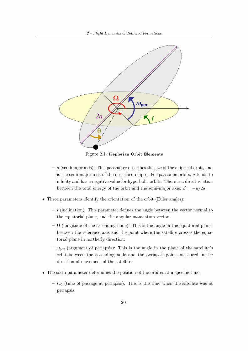
Figure 2.1: Keplerian Orbit Elements
– a (semimajor axis): This parameter describes the size of the elliptical orbit, and
is the semi-major axis of the described ellipse. For parabolic orbits, a tends to
infinity and has a negative value for hyperbolic orbits. There is a direct relation
between the total energy of the orbit and the semi-major axis: E = −µ/2a.
• Three parameters identify the orientation of the orbit (Euler angles):
– i (inclination): This parameter defines the angle between the vector normal to
the equatorial plane, and the angular momentum vector.
– Ω (longitude of the ascending node): This is the angle in the equatorial plane,
between the reference axis and the point where the satellite crosses the equa-
torial plane in northerly direction.
– ωper (argument of periapsis): This is the angle in the plane of the satellite’s
orbit between the ascending node and the periapsis point, measured in the
direction of movement of the satellite.
• The sixth parameter determines the position of the orbiter at a specific time:
– tτ0 (time of passage at periapsis): This is the time when the satellite was at
periapsis.
20

2 – Flight Dynamics of Tethered Formations
The parameter tτ0 is used to relate a particular time to a particular position. Other
parameters can be used for this purpose. This is why, often in the literature, some alter-
native parameters are used. The most commonly used are θ0 which is the true anomaly at
a given time t0, or M0 which is the mean anomaly at a given time t0. The true anomaly
parameter is the angle in the plane of the satellite between the periapsis and the satellite.
It can be seen in Fig. 2.1. The mean anomaly is a ”scaled” parameter of true anomaly
in the sense that the Mean Anomaly evolves at constant rate during a particular period
as opposite to the true anomaly that has a non-constant rate. In circular orbits, have the
same value and in elliptical orbits, they have the same value at periapsis and apoapsis.
The mean motion is represented with the variable n and measures the average rate of
a Keplerian orbit. In the case of a circular orbit n is the constant angular rate in the orbit
plane. A Keplerian orbit satisfies the equation:
n =
õ
a3=
2π
TO(2.2)
where TO is the Orbital Period. One of the advantages of using the orbit element approach
to model the orbit of a satellite is the lack of need to integrate any differential equation
to determine the position of the satellite at a specific time. The position of the satellite
can be determined from the mean anomaly,
M(t) = M0 + nt = n(t− tτ0) = Ea − e sinEa (2.3)
where E is the eccentric anomaly and M is the mean anomaly. The conversion between
true anomaly θ and mean anomaly parameters is given by
tanθ
2=
√1 + e
1− e· tan
Ea2
(2.4)
Although the orbital elements are enough to define an orbit, they present singulari-
ties. For instance, the longitude of the ascending node is undefined for orbits with zero
inclination and the line of apsides is undefined for zero eccentricity (circular orbit). It is
possible to formulate differently the orbit elements in order to avoid these singularities.
The Equinoctial Lagrange Elements presented in Ref. [40] define six alternative orbital
elements to avoid these singularities [41].
An alternative formulation of orbital elements, consist in defining a set of canonical
orbital elements. The Delaunay elements are the canonical formulation of the Keplerian
21

2 – Flight Dynamics of Tethered Formations
Orbital Elements, and the Poincare elements are the canonical formulation of the Equinoc-
tial Lagrange Elements. The six Delaunay elements, as found in [42] are expressed as
lD = M gD = ωper hD = Ω
L =√aµ GD = L
√1− e2 HD = G cos i (2.5)
The following identities can be used to relate the true longitude L and mean longitude
λ parameters:
λ = MD + ωper + Ω
L = θ + ωper + Ω (2.6)
As stated before, these orbital elements have the property:
dL
dt=
∂H∂lD
dlDdt
= −∂H∂L
dGDdt
=∂H∂gD
dgDdt
= − ∂H∂GD
dHD
dt=
∂H∂hD
dhDdt
= − ∂H∂HD
(2.7)
where H is the Hamiltonian as shown in [38] and [43]. The advantage of using canonical
elements is that the Lagrange bracket matrix [38] is diagonal.
2.2 Dynamics of Relative Motion
Different alternatives are available to model the problem of formation flight in which there
is one or more agents linked through tethers, rotating around the Earth. The two-body
approach will be used as a basis to describe the relative equations of motion. On a first
approach, the relative motion of two orbiters can be derived by substracting the equation
of relative motion of two bodies (or a body and the reference orbit) and thus obtaining
the relative dynamics. However, as it will be shown in the sequel, there are other sets of
state variables more convenient to model the problem.
2.2.1 Equations of motion relative to a reference orbit
This section presents the derivation of the equations of motion of an orbiting body, ex-
pressed in the relative coordinates of a frame attached to a reference orbit. The Euler-
Lagrange approach will be used for the derivation. The background behind this approach
22

2 – Flight Dynamics of Tethered Formations
is widely explained in mechanics literature [37].
The Euler-Lagrange equations allow one to derive the equations of motion of a me-
chanical system, based on the expression of its kinetic and potential energy only, if the
system is conservative and all constraints are holonomic. Kinetic and potential energy
energy must be defined as a function of the so called generalized coordinates. General-
ized coordinates is the set of variables that define uniquely the configuration of a system.
Generalized velocities are the time derivative of generalized coordinates. Although it is
preferable that generalized coordinates are independent, this is not mandatory, but when
this happens, the number of generalized coordinates equals that of system degrees of free-
dom. Euler-Lagrange equations for a conservative system with holonomic constraints and
n degrees of freedom are written in the form:
d
dt
(∂T∂qj
)− ∂T∂qj
+∂V∂qj
= 0 (2.8)
where qj are generalized coordinates j = 1, ..., n. Variable T is the total kinetical energy
of the system and V its total potential energy. The advantage of this approach over other
methods is that the choice of the generalized coordinates is arbitrary. In some problems,
writing the equations of motion based on variables having special geometric properties can
be much simpler than using, for instance, Cartesian coordinates and/or lead to simpler
expressions for the equations of motion. Moreover, for a system with ideal holonomic
constraints, writing the equations of motion by means of Euler-Lagrange equations does
not require to express explicitly constraint forces.
In the applications considered in the present thesis, the orbital kinetic energy T is
calculated as the sum of kinetic energies of the parent bodies plus that of the agents. The
orbital potential energy V is the sum of the potential energies of the parent body plus that
of the agents.
Appropriate extensions of Eq. (2.8) exist for systems affected by non-conservative forces
(e.g. the Raleigh dissipation function can be used as a measure of the power dissipated
by non-conservative forces), or system with non-holonomic constraints or described by a
set of non-independent generalized coordinates (use of Lagrange multipliers). A detailed
derivation can be found in [37].
23

2 – Flight Dynamics of Tethered Formations
When analyzing formation flight problems, it is often convenient to describe the po-
sition of the deputies with respect to the parent body, or with respect to a predefined
reference orbit. For this reason it is convenient to describe the motion of the deputy with
respect to a non-inertial reference system centered in the parent body or the reference
orbit, and not the Earth.
Figure 2.2: Reference frames O and R
This approach is based on two reference systems. The inertial reference system (fixed
frame) O : I, J, K is Earth-centered with K pointing along the Earth’s spin axis, whereas
I and J lie on the equatorial plane. The I unit vector lies at the intersection of the (in-
ertially fixed) equatorial and ecliptic planes and J completes a right-handed triad. The
rotating or orbital reference frame, also known as Local Vertical Local Horizontal (LVLH)
is R : iR, jR, kR . In this frame, the iR axis points outwards in the radial direction from
the center of the Earth to the parent body, the kR axis is perpendicular to the orbital plane
along the angular momentum vector and the jR axis completes a right-handed orthogonal
triad. When the orbit is circular, jR is tangent to the direction of movement. The origin of
the LVLH frame coincides with the parent body position following a prescribed reference
orbit. In the absence of parent body, the center of the local reference frame is that of the
reference orbit.
The expression of the kinetic and potential energy (T and V respectively) depends
on the orbital parameters of the reference orbit and the position of the agent within the
24

2 – Flight Dynamics of Tethered Formations
LVLH frame, that is:
T =1
2
N+1∑i=1
mi(Rref · Rref) + Rref ·N∑i=1
mi(vi) +1
2
N∑i=1
mi(vi · vi)
= Torb + Rref ·N∑i=1
mi(vi) +1
2
N∑i=1
mi(vi · vi) (2.9)
and
V = −µN+1∑i=1
mi
Rref− µ
R2ref
N∑i=1
mi(iR · ri) +µ
2R3ref
N∑i=1
mi(ri · ri − 3(iR · ri)2)
= Vorb −µ
R2ref
N∑i=1
mi(iR · ri) +µ
2R3ref
N∑i=1
mi(ri · ri − 3(iR · ri)2) (2.10)
where the orbital components are grouped in terms Torb and Vorb. Vectors ri and vi
describe the position and velocity of deputy i in the LVLH frame. In these equations
N defines the total number of deputies, such that N + 1 is the total number of agents,
including the parent body. The following two sections describe how to derive the equations
of motion, taking into account two sets of generalized coordinates. In the first case, a set
of cartesian coordinates is used, whereas in the second case it is a set of polar coordinates.
The use of this approach requires writing the kinetic and potential energies in terms of
the chosen generalized coordinates.
Cartesian coordinates
When the position of the deputies with respect to the parent body is described in the LVLH
frame, the most obvious choice for this is to use q1, q2, q3, ..., qn = xj , yj , zj , ..., zN with
n = 3N , in the absence of constraints on the position of the N mass elements.
Assuming that the parent body (leader) follows a prescribed reference orbit Rp = Rref,
and letting Rd = Ri be the absolute position of a deputy (chaser) in the LVLH frame,
these position vectors are expressed in R as:
Rp = Rref · i
Rd = Rp + rd = (Rref + xd) · iR + yd · jR + zd · kR (2.11)
25

2 – Flight Dynamics of Tethered Formations
Assuming ωR/O = θ · K, the velocities of the leader and the follower(s) are given by:
Rp = Rp|R + ωR/O ×Rp = Rref · iR + θRref · jRRd = Rp + vd (2.12)
vd = rd|R + ωR/O × rd = (xd + θyd) · iR + (yd + θxd) · jR + zd · kR
where θ is the angular rate of the orbiting body, or true anomaly rate. After substituting
expressions (2.11) and (2.12) in (2.9) and (2.10) with Rref = Rp, ri = rd and vi = vd,
the equations of motion for a particular deputy body d are obtained. Eliminating the
subscript d for convenience, the equations of motion for a deputy body, are
x− 2θ(y − y(Rref/Rref))− xθ2 = −µ(Rref + x)/R3ref
y + 2θ(x− x(Rref/Rref))− yθ2 = −µy/R3ref (2.13)
z = −µz/R3ref
Circular reference orbit
In order to simplify the model, some assumptions can be taken in addition to those asso-
ciated to Eq. (2.1). When
• Rref >>‖ ri ‖
• The parent body of the formation follows a circular orbit, which implies Rref is
constant and the eccentricity is zero, e = 0.
the so-called Hill-Clohessy-Wiltshire (HCW) equations are derived [44]:
x− 2ny − 3n2x = 0
y + 2nx = 0 (2.14)
z + n2z = 0
where, for a circular reference orbit, the true anomaly rate θ is replaced by the constant
mean orbital rate n. Notice that the kR component of the motion is decoupled from
displacements in the iR − jR plane. When incorporating the presence of external forces,
26
2 – Flight Dynamics of Tethered Formations
HCW equations achieve the form:
x− 2ny − 3n2x = fx/mi
y + 2nx = fy/mi (2.15)
z + n2z = fz/mi
In the absence of external forces, an analytical solution to (2.15) can be found:
x(t) = A0 cos(nt+ ka) + xk0
y(t) = −2A0 sin(nt+ ka) + yk0 − (3/2)ntxk0 (2.16)
z(t) = B0 cos(nt+ kb)
where ka, kb, A0, B0, xk0 and yk0 are integration constants. The solution shows a secular
term in the second equation. In order to eliminate secular drift, it can be easily shown that
xk0 must be zero, and therefore the following initial condition must satisfied y0 = −2nx0.
Otherwise, the relative orbit will not be bounded and the deputy drifts away from the
center of the frame. References [17] and [45] study the effect of incorporating eccentric
orbits using the HCW approach.
Elliptical reference orbit
Equation (2.13) is valid for a generic Keplerian orbit. For a Keplerian elliptical orbit, the
following equations hold [38]:
R =a(1− e2)
ξθ = ξ2
õ
a3(1− e2)3ξ = (1 + e cos θ) (2.17)
After linearizing the gravitational term as in [17] and defining the equations of motion
in terms of e and θ, the equations of relative motion in R achieve the following form:
x− 2θy − θ2x− θy + 2n2(ξ/(1− e2))3x = fx/mi
y + 2θx− θ2y + θx+ n2(ξ/(1− e2))3y = fy/mi (2.18)
z + n2z = fz/mi
This equation provides a valid alternative to describe the linearized relative motion
with respect to an elliptical reference orbit. Lawden derived a model and obtained an
analytical solution for the relative motion in the absence of external forces [46] using
27

2 – Flight Dynamics of Tethered Formations
Eq. (2.18), taking true anomaly as independent variable. Unfortunately, the analytical
solution derived by Lawden includes an integral which presents singularities for certain
values of the eccentric anomaly. Tschauner and Hempel derived a similar set of equations
of motion for relative motion with respect to an elliptical orbit, scaling state variables with
respect to the radius of the parent body [47]. A significant contribution was provided by
Carter [48], who refined Lawden’s solution by providing an alternative integral, which is
not affected by the above mentioned singularities. A historical perspective on the deriva-
tion of this model can be found in Ref. [49].
Reference [50] derives a third-order expression, for both in-plane and out-of-plane dy-
namics of the solutions of the elliptic HCW non-linear equations. The solutions are in
powers of two amplitudes but exact in eccentricity (i.e. accuracy is good also for high
eccentricities).
Reference [17] provides a technique for evaluating initial conditions for the elements of
the cluster such that deputies do not present secular motion, and the necessary conditions
that provide periodic solutions, with deputies returning back to the initial states at the
end of each orbit.
Polar coordinates
One of the advantages of using the Lagrangian approach is the freedom of choosing the
set of generalized coordinates that better suits each particular problem. The geometry of
the system in some cases can make some choice preferable to another. This section focus
on the derivation of equations of motion using polar coordinates.
The choice of variables is based on the formation orientations presented in Ref. [13].
The cluster orientations used in this reference are known as In-plane and Earth-facing.
Depending on the cluster configuration a different pair of polar coordinates is chosen to
represent the motion.
For the In-plane configuration, deputies are nominally in the orbit plane. The orbital
plane is defined by axes iR and jR of the LVLH reference frame. For this reason, vari-
ables l, α and β are used to represent the position as indicated in Fig. 2.3(a), where l
defines the distance to the parent body, variable β is used to monitor the out-of-plane
elevation from the nominal plane (roll motion), and α will express the in-plane angular
28

2 – Flight Dynamics of Tethered Formations
motion of the deputy around the parent body (pitch motion) contained in the orbital plane.
Figure 2.3: Polar coordinates in LVLH reference: in-plane (a) and Earth-facing (b)cases
In the Earth-facing configuration, deputies are intended to lie in the plane defined by
jR and kR. Following the same criteria as before, variable l defines the distance to the
parent body, variable α∗ express the in-plane angular motion contained within the normal
plane facing the Earth, and β∗ is used to represent the out-of-plane motion with respect
to the normal plane facing the Earth as indicated in Fig. 2.3(b).
ri = (li cosα cosβ)iR + (li sinα cosβ)jR + (li sinβ)kR (2.19)
ri = (li sinβ∗)iR + (li sinα∗ cosβ∗)jR + (li cosα∗ cosβ∗)kR (2.20)
For the In-plane case, the relative position vector of the i-th deputy is expressed in
terms of l, α and β variables in the form of Eq. (2.19), whereas for the Earth-facing case
one gets Eq. (2.20) in terms of l, α∗ and β∗. The derivation of the equations of relative
motion in terms of the cited variables then follows the procedure used for writing the
equations in the Cartesian frame.
In Ref. [13] this is done for different cluster structures. The potential energy due to
elasticity and the generalized damping force, depend of the geometry of the links defining
the cluster. For this reason it is necessary to perform a complete new derivation of the
equations of motion for every formation geometry.
29

2 – Flight Dynamics of Tethered Formations
2.2.2 Relative equations of Motion based on Orbit Elements
The orbit elements allow to define the orbit of a single orbiter. For the flight formation
problem, it is necessary to define the relative position from a deputy body with respect to
a parent body orbiting the Earth. For this reason, it is convenient to define the relative
motion of two satellites through the relative orbit element vector:
X = Xd −X = (δa, δe, δi, δΩ, δωper, δθ) (2.21)
The choice of the six orbit elements is not constrained to these shown in Eq. (2.21).
As stated before, the derivation of all the X variables does not require the integration of
any equation of motion. A further advantage provided by using the formulation in orbit
element differences is that in some cases it is possible to have a notion of the relative
dynamics directly from the values. For instance, through the difference values of δi and
δΩ it is possible to have an idea about the relative out-of plane motion between deputy
and chaser.
In the absence of relative drift, vector X should be constant. However, due to external
influences such as external perturbations it may be possible that a secular drift is presented
between orbiter and chaser, and therefore ˙X /= 0. Reference [51] estimates the evolution
of the relative motion between deputy and chaser due to different orbital energies, due to
atmospheric drag and due the J2 perturbation.
Reference [52] uses the relative orbit element formulation to define a control law with
the purpose of reestablishing a J2 invariant orbit for a deputy-chief pair. This reference
takes into account the results found in [53] where conditions are defined to remove the
secular drift between two orbiters. Reference [54] defines a strategy for satellite relative
orbital design using least squares methods.
It is possible to define a mapping between the difference among parent and deputy
expressed in terms of orbit elements variables and the coordinates in the HCW frame
[55], [56]. Reference [57] derives in detail the expression taking into account different
30

2 – Flight Dynamics of Tethered Formations
hypotheses. The mapping, assuming chief orbits with small eccentricity is as follows:
x(θ) ≈ (1− e cos θ)δa+ (ae sin θ/√
1− e2)δM − a cos θδe
y(θ) ≈ (a/√
1− e2)(1 + e cos θ)δM + a(1− e cos θ)δωper
+ a sin θ(2− e cos θ)δe+ a(1− e cos θ) cos iδΩ (2.22)
z(θ) ≈ a(1− e cos θ)(sin θδi− cos θ sin iδΩ)
The mapping is written using the true anomaly θ as independent variable. Using
Kepler’s equations it is possible to relate θ and time. Reference [58] proposes a positioning
hybrid control law that takes into account both the orbit element representation, and the
mapping to the Cartesian coordinates shown in Eq. (2.22).
2.2.3 Comparison of orbital models
The main advantage of the Lagrangian approach, using Cartesian coordinates as gener-
alized coordinates, is that the representation of position in the LVLH is straightforward.
This property is specially interesting when using elastic tethers when one needs to com-
pute distances to determine elongations. The use of polar coordinates is convenient only
for clusters where tethers have a radial geometry with respect to the parent body. In this
particular case, defining lj as a generalized coordinate is very convenient, but in the case
of tethers connecting external deputies, the calculation of distances is less straightforward
than when using Cartesian coordinates.
One of the most interesting features of using orbital elements to represent the position
of an orbiting body is that it is possible to determine its position using algebraic equations
only, without the need of integrating differential equations as it is the case in the HCW
approach. On the other hand, when incorporating additional forces, like those of spring-
dampers or those arising from perturbations, this property vanishes and one still needs
to integrate a set of six differential equations as it happens in the HCW case. As it will
be explained later, it is possible to use the orbital elements formulation and still define
external accelerations in the LVLH frame which is a convenient property. However, the
set of differential equations is non-linear as opposite to the linearization used in the HCW
case.
31

2 – Flight Dynamics of Tethered Formations
2.3 Effects of Orbit Perturbations
As introduced before, Eq. (2.1) does not include effects like the gravity attraction from
the Moon or the Sun. It does not include neither solar radiation pressure nor tidal ef-
fects. They will be incorporated within the model by defining external perturbations to
the motion from the ideal Kepler solution. Table 2.1, taken from [59], presents a list of
the most important perturbations affecting a satellite orbiting a Low Earth Orbit, along
with an order of magnitude showing their relevance. Earth’s gravitational field provides a
term of comparison for all the perturbing accelerations. Note that many perturbing terms
strongly depend on the orbit and can achieve different importance in different operating
conditions, e.g. atmospheric fiction, which is moderate in LEO below 300 km, becomes
totally negligible above 500 km of altitude.
Table 2.1: Perturbative accelerations acting on a LEO orbit
Conservative Force Acceleration (m/s2)Earth’s gravitational field ≈ 10Earth’s oblateness (J2) ≈ 10−2
Earth’s oblateness (J4) ≈ 10−4
Lunar attraction ≈ 10−6
Solar attraction ≈ 10−7
Planetary attraction ≈ 10−10
Tidal Effects ≈ 10−6
Relativisitic effects ≈ 10−8
Non-Conservative Force Acceleration (m/s2)Atmospheric friction ≈ 10−4
Solar radiation pressure ≈ 10−7
Albedo effect ≈ 10−8
Chapter 4 studies the effect of the J2 perturbation on tethered clusters orbiting in LEO.
This is the most significative perturbation in this scenario as shown in Tab. 2.1. The next
highest perturbation is atmospheric drag, which is two orders of magnitude smaller. In
addition to the fact that is smaller, it is also worth to remark that for Earth-facing clusters
the effect on the relative position of the agents should not be noticeable due to the fact
that all agents lie approximately at the same altitude. For in-plane clusters, the length of
the tethers is small compared with the altitude, and due to the spinning configuration, all
cluster members experience the same drag profile on each rotation of the formation. For
these reasons it is expected that the effect of atmospheric drag on the relative position of
32

2 – Flight Dynamics of Tethered Formations
the agents of the cluster is negligible.
The equations of motion assuming a perturbation causing an acceleration adist achieve the
form:
R =µ
R2
R
|R|+ adist (2.23)
Reference [55] describes in detail Cowell and Encke’s methods to calculate the orbit
of a body under perturbation effects. Both methods introduce the concept of osculating
orbit and reference orbit. A perturbation acting on an orbiting body affects its position,
therefore altering the original keplerian orbital parameters. The osculating orbit is the
orbit that at each instant has the orbit parameters determined from the current values of
position and velocity vectors.
According to Encke’s method, the perturbed orbit is calculated as the sum of the unper-
turbed orbit trajectory (calculated using the two-body Kepler solution) and the deviation
from the reference orbit due to perturbations. This method proposes a way to estimate
the deviation with respect to the unperturbed orbit, and therefore allowing to calculate
the position of an orbiter as the sum of the deviation plus the nominal unperturbed orbit.
This method was used when computing power was limited, and approximative techniques
had to be used for orbit computation.
According to Cowell’s method, the perturbed orbit is calculated integrating directly
Eq. (2.23), that is, the nominal Keplerian model plus the sum of perturbation accelerations.
2.3.1 Perturbations in Equations of Motion
Perturbations in Orbit Element Approach
Some perturbations are conservative, and therefore can be expressed as a disturbance
potential that depends only on the distance R. The acceleration adist is created as the
result of a disturbance potential VR(R), where:
adist = ∇VR(R) (2.24)
As reported in [38], is it possible to obtain the variation in the orbit elements as a
33

2 – Flight Dynamics of Tethered Formations
function of this potential. This leads to the Lagrange Planetary Equations (LPE):
dΩ
dt=
1
nab sin i
∂VR∂i
di
dt= − 1
nab sin i
∂VR∂Ω
+cos i
nab sin i
∂VR∂ωper
dωper
dt= − cos i
nab sin i
∂VR∂i
+b
na3e
∂R
∂e(2.25)
da
dt=
2
na
∂VR∂M0
de
dt= − b
nea3∂VR∂ωper
+b2
nea4∂VR∂M0
dM0
dt= − 2
na
∂VRa− b2
nea4∂VR∂e
One of the advantages of using a canonical representation for orbital elements is that
the Lagrange matrix is diagonal. The derivation using the Lagrange brackets, however
requires that the disturbance can be expressed in the form of a potential, and therefore
not admiting disturbances caused by non-conservative forces. In [39] it is shown that
this restriction is indeed not necessary, and that it is possible to express the variational
equations in a form known as the Gauss Planetary Equations (GPE) which include a
general acceleration expressed in the orbital frame coordinates. The definition of the
GPE equations in the LVLH frame coordinates leads to the following set of 6 first order
differential equations:
da
dt=
2a2
he sin θaiR +
p
RajR
de
dt=
1
h(p sin θaiR + ((p+R) cos θ +R · e)ajR)
di
dt=
r cos θ
hakR
(2.26)
dΩ
dt=
R sin θ
h sin iakR
dωper
dt= − 1
hecos θpaiR +
1
he(p+R) sin θajR −
R sin θ cos i
h sin iakR
dM
dt= n+
b
ahe(p cos θ − 2R · e)aiR − (p+R) sin θajR
where p = a(1 − e2), the modulus of angular momentum is h =√µp, and R is the
distance of the body to the center of the Earth. In this expression, aiR , ajR , akRare
the accelerations expressed in the local LVLH frame. This representation is convenient
since tether forces are easily expressed in a Cartesian coordinate system, and the generic
34

2 – Flight Dynamics of Tethered Formations
expression of the acceleration allows incorporating non-conservative forces such as the
damping force present in tethers.
Perturbations in the HCW approach
The inclusion of external forces (including perturbations), in the model of relative motion
is straightforward as it can be seen in Eq. (2.15). Forces due to a perturbation acting on
satellite are directly expressed in terms of components in the LVLH frame on the RHS of
the same equation.
2.3.2 Implementation of the J2 Perturbation
The Earth’s gravitational potential VE , is often represented using spherical harmonics
that model the irregularities in the Earth’s shape [38]. The potential function VE is com-
posed as the sum of terms that describe zonal, sectorial and tesseral spherical harmonics
that fit an accurate representation of the gravitational potential. The J2 harmonic is the
lowest-order zonal harmonic Earth’s oblateness. It accounts for Earth’s bulge around the
equator. It’s magnitude is by far the most relevant. For this reason, the effect of the
so-called J2 perturbation on tethered formations is analyzed in this study.
In order to simulate the effects of J2 potential over a cluster of satellites various ap-
proaches are available. The first option is to define a model based on Keplerian orbit
elements as state variables. In this nonlinear model, the effect of J2 perturbation can be
incorporated as shown in Ref. [38]. The presence of elastic forces due to tether tension
between pairs of agents can be included in the model in the form of external forces acting
on each agent of the formation, where the tension depends on the distance between the
agents connected by the considered tether.
J2 perturbation in Orbit Element approach
According to [60], the perturbation function VR(R) due to the J2 acceleration is:
VR = −J22
µ
R
(ReR
)2
(3 sin2 θ sin2 i− 1) (2.27)
The acceleration component obtained from the gradient of VR, projected in the LVLH
35
2 – Flight Dynamics of Tethered Formations
frame, are given by
aiR = −3
2
µJ2R2e
R4
(1− 3/2 sin2 i · (1− cos 2θ)
)ajR = −3
2
µJ2R2e
R4sin2 i sin 2θ (2.28)
akR= −3
2
µJ2R2e
R4sin i cos i sin θ
From these equations it can be clearly seen that for a given longitude, the perturbation
function vanishes at Earth’s poles, and reaches its maximum at the equator.
In order to take into account the J2 perturbation, Eqs. (2.27) and (2.28) and can be
substituted into Eqs. (2.25) and (2.26). It can be shown that the J2 perturbation does
not introduce any secular drift for orbit elements a, e and i. For the purpose of formation
control, in order to ensure that the perturbation affects the formation orbiters in the same
way, Ref. [53] defines the conditions necessary to avoid secular drift between agents under
the action of the J2 perturbation.
Based on the cited article, Ref. [61] studies the problems associated to near-circular
and near-polar orbits of the parent body. Reference [51] by one of the same authors,
explores further the incorporation of secular drifts in the formation due to unequal orbit
energies and atmospheric drag.
References [62] and [63] evaluates the effect of the J2 perturbation through a state-
transition-matrix. Reference [64] compares different motion models taking into account
the J2 perturbation.
J2 perturbation in HCW equations
Reference [16] presents the derivation of the linearized equations of motion of an orbiting
satellite, under the influence of the J2 potential, with respect to a reference orbit. This
paper analyzes the effect due to the J2 perturbation for each one of the LVLH axes and
derives a set of equations of motion in the LVLH frame. To do this, first one needs to
incorporate the effect of the perturbation on the orbiting body acceleration, and then
modify the reference orbit accordingly in order to avoid a secular drift between the orbiter
and the reference orbit.
36

2 – Flight Dynamics of Tethered Formations
The equations of motion are:
r + 2ω × r + ω × r + ω × (ω × r) = R− Rref (2.29)
The relative position of the satellite with respect to the reference orbit in the LVLH
frame is denoted by r = R−Rref, where R is the position vector of the satellite and Rref
that of the reference orbit. The acceleration for a deputy is:
R = g(Rref) +∇g(Rref)r + J2(Rref) +∇J2(Rref)r (2.30)
This equation is a differential equation with time varying coefficients, because the
expression of ∇J2(Rref) is a function of latitude. In order to obtain an autonomous (i.e.
time-invariant) set of equations, an approximation with constant coefficients is derived,
using the average of ∇J2(Rref), over one period, equal to
1
2π
∫ 2π
0∇J2(Rref)dθ =
µ
R3ref
+
4sJ 0 0
0 −sJ 0
0 0 −3sJ
(2.31)
with sJ = (3J2R2e/8R
2ref)(1 + 3 cos 2i)
instead of its exact value. The modified set of equations poses two problems. On one
side, the perturbation terms J2 and ∇J2(Rref) that affect satellite relative position are
computed over the reference orbit, Rref, which is also subject to the effects of the J2 per-
turbation. This fact needs to be accounted for to prevent the error between the effective
orbit and the reference one to grow up unboundedly, thus leaving the small perturbation
range necessary for linearization.
The reference orbit Rref should be redefined in such a way that no secular drift is
produced between the orbiting body and the reference orbit. The analysis of the motion
within the LVLH frame is as follows:
• For the radial direction, no drift is expected considering that no secular drift is
produced on orbit semi-major axis, a, and eccentricity, e [51]. Therefore, taking
the time average of the J2 potential gradient doesn’t lead to any secular loss of the
accuracy in the predicted motion.
• Changes in the tangential direction due to the J2 perturbation can be caused by
37

2 – Flight Dynamics of Tethered Formations
changes eccentricity or orbital period. Since the first case is not possible, it is
sufficient to choose an orbital period for the satellite equal to that of the reference
orbit. To avoid secular drift, the initial condition of the satellite will have to be
calculated specifically, as it will be shown in the sequel.
• The dynamics in the cross-track direction is more complicated, due to the secular
change in the longitude of the ascending node caused by the J2 perturbation. These
dynamics require both a correction of the reference orbit to compensate for the nodal
drift and a redefinition of the cross-track dynamics.
After correcting the reference orbit period, and its nodal drift, the acceleration of the
corrected reference orbit is calculated as:
Rref = g(Rref) +1
2π
∫ 2π
0J2(Rref) dθ + [J2(Rref) · kR]kR (2.32)
The reference angular velocity is replaced by the value ω = nc z, where n is the mean
motion and c =√
(1 + s). The following equations are thus derived in [16]:
x− 2ncy − (5c2 − 2)n2x = −3n2J2(R2e/Rref) ·
·1/2− [3 sin2 iref sin2 (kt)/2]− [(1 + 3 cos(2iref)/8]
y + 2ncx = −3n2J2(R2e/Rref) sin2 iref sin kt cos kt (2.33)
z + (3c2 − 2)n2z = 0
with k = nc+3õJ2R2
e
2R7/2 cos2 iref and x, y and z Cartesian coordinates in the LVLH frame.
These equations do not accurately capture the dynamics of the cross-track motion,
thus presenting a second problem when i /= 0 due to the averaging of ∇J2(Rref). The
approximation makes the effect of the potential symmetric with respect to the normal to
the orbit plane, rather than to the vector pointing towards the North pole. In order to
solve this issue, it is sufficient to reformulate the cross-track dynamics, that is, the third
equation in Eq. (2.33), as
z + p2qz = 2plpq cos(pqt+ pφ) (2.34)
where the derivation of parameters pl, pq and pφ is presented in detail in [16].
38

2 – Flight Dynamics of Tethered Formations
As in the Hill-Clohessy-Wilthsire equations, the cross–track and the in-plane dynamics
are uncoupled, making it possible to solve the equations separately. In some special cases
it is possible to obtain a bounded analytical solution, by imposing restrictions on the initial
velocity conditions. Reference [16] also provides the equations that model the orbit of a
satellite motion relative to a second satellite, in which case the equations are formulated
in terms of ∆x, ∆y, and ∆z variables, that is,
x = (x0 − pα) cos(nt√
1− s) +
√1− s
2√
1 + sy0 sin(nt
√1− s) + pα cos(2kt)
y = −2√
1 + s√1− s
(x0 − pα) sinnt√
1− s+ y0 cos(nt√
1− s) + pβ sin(2kt)
z = (plt+m) sin(pqt+ pφ) (2.35)
pα = −3J2R2en
2
4kRref
(3k − 2n√
1 + s)
n2(1− s)− 4k2
pβ = −3J2R2en
2
4kRref
2k(2k − 3n√
1 + s) + n2(3 + 5s)
2k(n2(1− s)− 4k2)sin2(iref) (2.36)
The initial conditons on the velocity of the deputy that ensure that no secular drift is
presented with respect to the reference orbit, are the following:
x0 = y0n
(1− s
2√
1 + s
)y0 = −2x0n
√1 + s+
3J2R2en
2
4kRrefsin2 iref (2.37)
Reference [65] evaluates in detail the results of [16]. Reference [66] derives a model
which includes the effect of atmospheric drag, together with J2 perturbation.
2.4 Tether Models
Several approaches are available in the literature for modeling tether dynamics. When
tether elasticity is neglected, the system is rigid and the results for gravity-gradient sta-
bilized rigid bodies derived in [67] can be applied. When elasticity is taken into account,
the model may take incorporate different features depending on the degree of fidelity re-
quired, and the specific characteristics of the mission scenario. Richer models improve the
accuracy of the results, usually at the expense of a higher computational load. There are
39
2 – Flight Dynamics of Tethered Formations
different features than can be taken into account for tether modeling:
• Elasticity: This property implies that the tether allows longitudinal stretching
beyond its natural length.
• Mass: The inclusion of tether mass in the model, requires a model for mass dis-
tribution, either a continuous model (based on the string equation), or a discrete
model based on massless stretches connecting concentrated masses.
• Extensibility: The variable unstretched length is needed to represent deploy-
ment/retrieval operations.
In the following sections, the implementation of each one of the cited features will be
described.
2.4.1 Elasticity Model
A tether elongated beyond the nominal unstretched tether length l(0) exhibits an opposit-
ing restoring force. This force is a combination of an elastic restoring force (such as that of
a linear spring) and a damping force that depends on the tether elongation rate (damping
effect). Materials showing this behavior are known as visco-elastic materials [68]. There
are different variants of visco-elastic models depending on the specific arrangement of the
model combining spring and damper: these two can be arranged in series, in parallel or a
combination of both.
According to the Kelvin–Voigt visco–elastic model the spring and damper are set up
in parallel. In this case the stress-strain relationship is represented as:
T = −Et · ε− Ct · ε (2.38)
where Et is the material Young’s modulus, Ct is the coefficient of internal friction and ε
is the strain. For some materials and for some specific applications, accurate modeling
of Ct needs to take into account structural (or hysteretic) damping [68]. This approach
takes into account an hysteresis cycle in the σ–ε plane, and the effect of the frequency of
oscillation. The value of Ct can be calculated as:
Ct =Et · ηt
Ωt(2.39)
where ηt is the loss factor (that depends on the specific characteristics of the material)
and on the oscillation frequency Ωt. Results show that for a space tether, the value of Ct
40
2 – Flight Dynamics of Tethered Formations
can be assumed constant and thus independent from frequency.
For a space tether, the visco–elastic properties of the tether material are assumed to be
those of a Kelvin–Voigt material model, which consists of a spring and a damper connected
in parallel. For a massless tether connecting agents i and j, the force exerted on agent i
and agent j can be calculated as:
f i,tens = EtAt · εj,i · ej,i + Ct · εj,i · ej,i if ∆lj,i > 0
f j,tens = −f i,tens(2.40)
where Et is the tether material Young’s modulus, At the area of the section of the tether
and Ct the damping constant. Versor ej,i = (rj − ri)/lj,i defines the direction connecting
agents j and i normalized by the tether length lj,i = |rj−ri|. Term εj,i = ∆lj,i/l(0)j,i defines
the strain between the j–th and i–th bodies, with an elongation ∆lj,i = lj,i − l(0)j,i , being
l(0)j,i the tether nominal unstretched length. Expanding Equation (2.40) leads to:
f i,tens =EtAt
l(0)j,i
·∆lj,iej,i +Ct
l(0)j,i
[ej,i · (vj − vi)− l(0)j,i ·
lj,i
l(0)j,i
]ej,i if ∆lj,i > 0 (2.41)
Grouping terms in this equation leads to
f i,tens = kt · Sj,i · ej,i + ct ·Dj,i · ej,i if ∆lj,i > 0 (2.42)
where kt and ct are the tether elastic and damping coefficients. Note that if the elonga-
tion ∆lj becomes equal or less than zero, the cable does not transmit any force (“slack”
condition) and so no action is present between the connected masses and only the gravity
gradient force drives their motion.
2.4.2 Effects of tether mass
Modeling transversal deflections requires taking into account the mass of the tether, in
order to determine the effect of the gravitational field over the mass distribution of the
tether. For this purpose there are two alternatives: A model based on the string equation
taking into account a constant density string, or a discretized model composed of massless
stretches connecting discrete lump masses.
41

2 – Flight Dynamics of Tethered Formations
Continuous Models
References [69], [70] and [71] present a theoretical model that describes tether dynamics
based on the string equation. This model determines the governing equations of an ar-
bitrary mass element ρ ds the teher of the tether, as well as the dynamics of the tether
ends. The modified string equation takes into account gravitational forces:
ρ∂2R
∂t2=∂f s,tens∂s
− ρµRR3
+ f s,grav (2.43)
where s is a curvilinear abcissa counted along the string. Considering that tension force
is always tangent to the thread line, it is
f s,tens = T · tR with tR =∂R
∂s
∣∣∣∣∂R∂s∣∣∣∣−1
the magnitude of tension T is defined from the elasticity law considered for each specific
tether material, and TR is the tangent unit vector. The equations of motion at the tether
endpoints a and b can be written as:
ma(t)d2Ra
dt2= tR,a
[Ta − ρ(sa)la
(dsadt
)2]−ma(t)
µRa
R3a
+ fa,grav (2.44)
mb(t)d2Rb
dt2= −tR,b
[Tb − ρ(sb)lb
(dsbdt
)2]−mb(t)
µRb
R3b
+ f b,grav (2.45)
where la and lb are the extension of the tether at endpoints.
ta = Et(sa)(la − 1) ; la =
∣∣∣∣∂R∂s∣∣∣∣a
(2.46)
tb = Et(sb)(lb − 1) ; lb =
∣∣∣∣∂R∂s∣∣∣∣b
(2.47)
Based on the model introduced above, Ref. [69] proposes simplifications that provide
different degrees of accuracy in the model. Reference [72] also analyzes tether dynamics
by exploiting the fact that tethers usually are very stiff.
Discretized Models
The purpose of discretized models is to address the problem by approximating the behavior
of the tether by a series of point-masses connected by straight massless spring–damper
42

2 – Flight Dynamics of Tethered Formations
elements. Although the use of continuous models is a valid choice for single tether systems,
discretized models alleviate the computational load, when multi-tethered systems are to
be dealt with. The first approach presented here consist in a model that defines a single
elastic massless elements linking pairs of deputies at the tether ends. For the massive
model, an approach is presented that allows discretization of tether by an arbitrary number
of stretches.
Massless model The massless model is the simplest one, and in this case the tether is
represented as a simplified massless spring–damper system connecting two agents at its
ends. For this case, the dynamics of the formation are expressed in the LVLH frame.
Under the assumption that cable mass is assumed zero, as in the analysis reported in
Ref. [13], the cables store elastic energy while remaining in a straight position under the
action of the tension exchanged between the bodies located at their extremities, induced
by gravity–gradient force and formation rotational motion.
The derivation of the equations of motion can be done using Lagrange equations.
The effect of the spring is taken into account as a potential energy due to elasticity, and
therefore included in the computation of the total potential energy. The damping force
shall be included as a dissipation function Qd,qj on the RHS of the equation since the
damping force is non-conservative.
d
dt
(∂T∂qj
)− ∂T∂qj
+∂V∂qj
= Qd,qj (2.48)
The elastic potential energy, consist of the gravitational term and the elastic term
V = VE + Velast.
Velast =
N∑i=1
1
2kt
(lt − l(0)t
)2; VE = −GMe
N∑i=1
mi
|Rp + ri|(2.49)
The Raleigh function for the damping force, can be written as:
Qd,qj = − ∂
∂qj
(N∑i=1
1
2ct l
2t
)(2.50)
where kt and ct are the elastic and damping constant respectively for the tether, lt the
length of a tether and lnom the nominal lenght of a tether. The expression of the kinetic
energy is obtained from Eq. (2.9).
43

2 – Flight Dynamics of Tethered Formations
The accelerations exerted by tethers linking pairs of deputies can be incorporated
directly in the equations of motion 2.48. Reference [13] uses this approach to study the
stability of different satellite cluster morphologies. Through a series of simplifications, and
assuming a circular orbit, the only orbital feature present in the equations of motion is
the orbital mean motion n. This reference also presents different cluster topologies estab-
lishing force links between the deputies. Each deputy will have three equations of motion
associated to the three degrees of freedom expressed by the chosen generalized coordinates
Massive model In this model, tether mass is introduced in the model by means of
a lumped–mass discretization. This approach was introduced in Ref. [14] and it consid-
ers tethers as a sequence of point-masses (beads) and massless springs-dampers. Refer-
ences [73] and [74] also make use of this formulation. It was applied also in Refs. [75] and
[76] in order study the behavior of orbiting large tethered structures without active control.
The total mass mt of a generic tether t is distributed over nb beads of equal mass,
mb = mt/nb. Each tether element is considered as a (small) orbiting body integrated in
the structure of the cluster. The tether is thus divided into a series of nb + 1 segments,
each one connecting two beads in the central portion of the tether, or a bead to either the
parent body or one of the deputies at its ends. Fig. 2.4 illustrates the concept.
For each tether segment, values for damping coefficient, cs, and stiffness, ks, are as-
signed considering a massless spring–damper system, where cs and ks are obtained by
imposing that the series of st = (nb+1) elastic elements provides an assigned value for the
equivalent stiffness and damping coefficients kt and ct of the whole tether over its length,
that is,
1/kt = (nb + 1)/ks ⇒ ks = st · kt (2.51)
1/ct = (nb + 1)/cs ⇒ cs = st · ct
where st is the number of segments, ks and cs are the elastic and damping constant of
each segment. The mass mt, the elastic constant kt, and the damping constant ct of the
tether are calculated using the following expressions:
mt = ρAtl ; kt = EtAt/l ; ct = Ct/l (2.52)
44

2 – Flight Dynamics of Tethered Formations
Figure 2.4: Stretches connecting beads, deputies and parent body
where ρt is the density, Et is the Young’s Modulus, Ct the damping constant of the tether
material, and At is the cross-section of the tether. Based on these parameters, and the
elastic model chosen, it is possible to calculate the force exerted by the tether at its ends.
Coupling of the movement among all the elements of the formation induced by tether
tensions is expressed through the components of the tether tension force f i,tens = fx,ii +
fy,ij + fz,ik on the RHS of Equation (2.14). The force exerted by a tether segment s
connecting elements a and b (two adjacent beads or a deputy and a bead) can be calculated
as:
fa,tens =EtAt
l(0)b,a
·∆lb,aeb,a +Ct
l(0)b,a
eb,a · (vb − va)− l(0)b,a ·
lb,a
l(0)b,a
eb,a if ∆lb,a > 0
= ks(b,a) · Sb,a · eb,a + cs(b,a) ·Db,a · eb,a
= −f b,tens
45

2 – Flight Dynamics of Tethered Formations
Comparison of Continuous and Discrete Model
Reference [77] analyzes the behavior of N coupled oscillators, which consist of an elastic
string attached to N particles of equal mass. The string has fixed ends. This reference
shows that as the number of point masses is increased and the length of the elements is
reduced, the equations of motion of the discretized model become equivalent to those of
the continuous string model. The number of vibration modes represented in the motion
will be as high as the number of oscillators N used in the representation of the model.
Oscillations of higher frequencies cannot be represented due to aliasing.
Reference [15] performs a modal analysis of the behavior of the tethers for a three-
dimensional cluster and presents a simulation showing the different vibration moldes. The
paper assesses the suitability of the bead model to represent tether dynamics.
It can be concluded that the discretized lumped-mass model is a valid representation
of the tether behavior. The accuracy in the representation of vibration modes wil depend
on the number of particles used in the lumped-mass model.
2.4.3 Tether Deployment and Retrieval
Most of the missions involving tethers require tether deployment and retrieval capabilities.
From the beginning of the mission it is necessary to unreel tethers in order to deploy the
cluster to its intended configuration. During mission operation it might be necessary to be
able to reel tethers for tension control purposes. Even if some natural configurations allow
keeping tether tension to a minimum level and thrusters play also a role in tether tension,
changing the tether natural length also allows modifying tether tension. In missions like
SPECS [35] it is necessary to have a formation with variable geometry. The change in the
shape is achieved by changing the tether natural lengths. The control of tether tension
and the control of tether length is complex problem, as it consist of a system with variable
mass due to the variation of the tether natural length. The modification of the tether
natural length also involves a change of its natural frequencies as explained before.
References [69], [78], [79], [72] and [80] derive the theoretical equations of motion for
deployment assuming a continuous string equations. Reference [70] presents different mod-
els of different complexity addressing the deployment/retrieval problem. References [81]
and [82] propose an optimal [83] control system for deployment and retrieval based on the
continuous model.
46

2 – Flight Dynamics of Tethered Formations
There are two main alternatives for reeling control when considering a lumped-mass
tether model. The first approach assumes a constant element length. This implies that
during deployment/reeling the number of beads will vary. The sudden addition or sup-
pression of a bead into the tether creates a discontinuity in the dynamics of the tether.
References [14], [84], [85] and [86] use this approach. In the instant when a new a massive
bead (having a certain velocity) leaves the spacecraft and it is incorporated in the tether,
momentum conservation needs to be taken into due account in order to determine the
state of the beads.
As an alternative, the model proposed in this thesis assumes a constant number of
beads and the length of the elements is changed during deployment/retrieval. When
deploying or retrieving a tether, the tether unstretched length parameter l(0) must be
updated as a consequence of the process of releasing or retrieving the cable. At the same
time, a new desired position must be defined for the deputies placed at the ends of that
tether, in order to keep the tether taut during the reeling process and at the final configu-
ration state. The change in l(0) and the new desired position for tether ends can be done
by tracking a ramp profile, the slope of which is used to regulate the rate of change. The
model is explained in more detail in Section 5.6.
2.4.4 Dynamics of a tether in orbit
The models presented so far are useful to define the most basic mechanical dynamics of a
tether without incorporating the gravity gradient force, or just by adding it as an external
force. The dumbbell model is often used in the literature. The advantage of this model is
that it incorporates explicitly the expression of the gravity gradient, and therefore allows
to study the dynamics of tethers in space. Different variants of the dumbbell model can
be derived, with various degrees of fidelity.
Tether dumbbell model
A first approximation for tether modeling is to consider a massive tether connecting two
point masses. A certain number of papers take into account this model, based on the
scenario of the TSS mission where a probe is connected to the Space Shuttle [87], [88].
Taking into account the kinetic and potential energy of the tether,
47

2 – Flight Dynamics of Tethered Formations
T = Torb +mel
2
2
[(α+ θ)2 cos2 β + β2
]+ma(mb +mt)
mTl2
V = Vorb +me
2
µ
R3l2(1− 3 cos2 α cos2 β
)(2.53)
(2.54)
where Torb, Vorb are kinetical and potential orbital energy:
Torb =mT
2
(R+R2θ2
); Vorb = −µmT
R
and ma, mb are the masses of the tether ends and mt is the tether mass tether and me
depends on the three values:
me = (ma(mb +mt/3) + (mt/3)(mb +mt/4)) /mT
mT = ma +mb +mt (2.55)
Variable ma is the mass of the spacecraft containing the tether reeling mechanism,
and therefore its value varies with time during tether deployment or retrieval operations.
As a consequence the value of mt also varies during tether reeling. The value of mb is
assumed constant. Variable α is the pitch angle (in-plane libration angle between tether
and local vertical), and β is the roll angle (out-of-plane angle with respect to the orbital
plane) as represented in Fig. 2.3. The first terms in T and V describe the orbital kinetic
and potential energy, whereas the remaining terms in each equation describe the energy
related to tether attitude and motion.
The equations of motion can be obtained using the Lagrange equations as in Eq. 2.8.
Using the generalized variables α, β, l:
cos2 β
[(α+ θ) +
(2l
lm∗1 − 2β tanβ
)(α+ θ) +
3µ
R3sinα cosα
]=
fαmel2
β +2l
lβ ·m∗ +
[(α+ θ)2 +
3µ
R3cos2 α
]sinβ cosβ =
fβmel2
(2.56)
l ·m∗ − l ·me
[β2 + (α+ θ)2 cos2 β +
µ
R3(3 cos2 α · cos2 β − 1)
]= fl
Where fi represent the generalized forces. A visco–elastic term modeling the tether
elastic behavior can be incorporated in the model through the fl term in Eq. (2.56), as an
48

2 – Flight Dynamics of Tethered Formations
external force.
Variable m∗ = ma(mb + mt/2)/(mTme), as shown in [89] and [90]. For non–circular
orbits, both R and θ can be written in terms of θ:
R =a(1− e2)
ζθ = ζ2
õ
a3(1− e2)3ζ = (1 + e cos θ) (2.57)
The model reported in Eq. (2.56) was used in many studies to analyze the behavior
of an orbiting tether. References that study the behavior on eccentric orbits, adopt true
anomaly θ as the independent variable. In order to study the behavior of an orbiting
tether different simplifications can be done to focus on those aspects of the dynamics
more relevant for the considered applicative scenario.
In a first approach only roll and pitch dynamics are modeled, and the longitudinal
dynamics are eliminated assuming a rigid tether, that is l = 0. In [94], both in-plane and
out-of-plane dynamics of a tether in an elliptic orbit are studied from an analytical and
numerical point of view.
To study the planar motion only pitch and longitudinal dynamics are considered, in
the absence of roll dynamics. This implies that β = 0 and β = 0. This scenario is studied
in several papers such as [90], [91], and [92].
To further simplify the model, only pitch motion can be studied, eliminating both roll
and longitudinal dynamics. This implies that l = 0, β = 0 and β = 0. This assumption
leads to the well known Beletsky equation, defined with true anomaly as independent
variable.
(1 + e cos θ)α′′ − 2α′ · e sin θ + 3 sinα cosα = 2e sin θ (2.58)
This case is studied in Refs. [93], [95], [96], [97] and [94]. Although the behavior of a
dumbbell in a circular orbit shows a regular behavior, when the eccentricity of the orbit
increases the pitch dynamics of the tether may exhibit a chaotic behavior. The size of the
chaotic region between libration and tumbling frequencies increases with eccentricity.
The same dynamics restricted to a circular orbit is studied in [89]. This implies that
l = 0, β = 0, β = 0 and n = θ. Reference [87] proposes a tension control law, based on the
49

2 – Flight Dynamics of Tethered Formations
linearization of the equations of motion. Reference [98] proposes an optimal controller for
set–point control of α, β, l. References [81] and [82] propose, respectively, a controller
for deployment and retrieval based on the model presented in Eq. (2.56).
Gravity-gradient stabilization
A single orbiting tether connected by two masses and aligned with the local vertical
exhibits a natural stable equilibrium. On the agent placed in the lowest end of the tether
(the one closest to the Earth), Gravity force is higher with respect to that exerted over the
agent on the furthest end. On the other hand, centrifugal force acting on the furthest agent
is higher than that on the lowest one. This fact creates a natural equilibrium state in which
the tether remains taut. In the absence of energy dissipation, a slight perturbation leads
to a pendulum-like oscillation of the tether with respect to the local vertical. Following
Eq. (2.56), the in–plane dynamics, in the absence of external forces is represented by:
α+ 3n2 sinα cosα = 0 (2.59)
In practice, a tether in such condition exhibits low amplitude libration due to external
perturbations to the non-uniformity of the gravity field. At the same time, friction and
atmospheric drag cause dissipation and thus damp out the oscillations.
Integrating this equation leads to:
α− 3n2 cos2 α = 2H (2.60)
which describes the pitch angular velocity as a function of the pitch angle. This equation
allows plotting a phase portrait with different trajectories as a function of the value of H,
as shown in Refs. [69] and [88]. The value H = 0 separates the regions of pendulum-like
libration (H < 0) and rotation (H > 0). Both references also study the coupled in-plane
and out-of-plane dynamics.
For elliptical orbits the Hamiltonian is not constant, and is possible to derive a similar
equation to represent the behavior by means of phase portraits. As shown in [88], the
tether behavior in elliptical orbits is chaotic.
50

2 – Flight Dynamics of Tethered Formations
Electrodynamic tethers
An electrically conductive tether in Low Earth Orbit can be used as a power generator
or as a motor generating thrust. The electrodynamic tether principles are described in
Ref. [1].
When no external current is applied, an electrical current is induced opposite to the
tether’s direction of motion. The current is perpendicular to the Earth’s magnetic field
and to the direction of motion. At the same time, an electromagnetic force is generated
opposed to the motion direction and the tether experiences drag. On the other hand, when
the current direction is reversed through an internal power source (a satellite battery or
a solar panel) thrust is generated along the tether motion and therefore the speed of the
tether is increased. The increment of tether energy results into an altitude increase.
References [99] and [100] provide insight and a review of the state of the art about
electrodynamic tethers dynamics. Reference [101] studies the effect of energy sources and
sinks on the design of an electrodynamic tether mission.
Provided that the scope of this thesis is focused only in non–conductive momentum
exchange tethers, electrodynamic forces will not be taken into account in the sequel.
Tether failure modes
One of the main hazards for a space tether mission in Low Earth Orbit is the chances that
one or more tethers are severed by micrometeorites or space debris. The main purpose of
the TiPS mission was to prove the long-term survivability of a space tether.
Reference [102] presents a collision study based on the failed TSS mission. This paper
shows a methodology for estimating the probability of tether failure due to debris, and
concludes that while it is likely that the tether collides with several particles less than 0.1
mm, the probability of colliding with large objects is small.
Reference [103] studies the survival of a double–strand tether while performing an
active debris removal mission consisting of de-orbiting an artificial satellite. A debris flux
is assumed as a function of altitude during the whole mission. The paper concludes that a
satisfactory mission success probability is achieved. Reference [104] also studies the debris
impact collision probability for a double–strand tether. The study concludes that even
51

2 – Flight Dynamics of Tethered Formations
though it is more probable to be hit, the probability of being severed is much lower than
that of a single-strand tether.
Tether materials
Space tethers shall made of materials be as light as possible. Some missions require de-
ploying tethers of several kilometers, and the cluster alternatives require often multiple
tether links between the agents of the cluster. If the tether material has a density too
high, the overall excessive tether mass on each agent will be excessive (having then an im-
pact on satellite fuel consumption), the deployment and retrieval manouvers will require
more power, and the bending of the tethers due to the gravitational force will affect the
whole cluster dynamics. At the same time, tether materials shall have high tensile stress
strength in order to transmit link forces between agents, and in order to support tension
peaks during cluster reorientation manouvers.
Table 2.2 provides a list of suitable material candidates for tethered clusters based on
the data provided in Refs. [69] and [105]. The first column defines the density ρ, and the
second column the tensile strength S∗ of the material. The third column shows the tether
break length in orbit calculated as,
L∗ =1
n
√2S∗
3ρ(2.61)
where the mean orbital period n is taken for a geosynchronous orbit. This is the maximum
length that the tether can withstand its own weight in orbit. It is a good metric to assess
suitability, since its value increases with the ratio between tensile stress and density. From
the presented results, it can be seen how the most common metallic materials clearly fall
behind in properties with respect to fibers and crystals. Although crystals present better
tensile stress than fibers, they are heavier and their practical use is impeded by to other
factors such as cost of manufacturing.
Within the literature the most usual choices for non-conductive tether materials are
Kevlar® and Spectra. The former is an aramid fiber of which two variants exist: Kevlar®
29 and Kevlar® 49. According to the manufacturer datasheet [106], both types present
the same density and tensile stress. References [107], [106] and [66] provide details on the
properties of this material. Several other references [74], [13], [89], [108], [109], [1] and
[78] consider Kevlar® a suitable material for tether space applications. According to Ref.
[110], Spectra generates less particles during deployment and is more resistant to atomic
52

2 – Flight Dynamics of Tethered Formations
Table 2.2: Tether material characteristics
Material ρ (g/cm3) S∗ (GPa) L∗ (103km)
WiresAluminium 2.7 0.6 5.3Stainless steel 7.9 2.0 5.7Titanium 4.6 2.25 7.9
FibersNylon 1.14 0.48 7.3Glass E 2.55 3.5 13.2
Kevlar® 29/49 1.45 2.8 15.7Quartz 2.19 6.0 18.7Spectra 2000 0.97 3.0 19.8
CrystalsGraphite 2.2 20 34.1Diamond 3.5 54 44.4
oxygen, but has less heat resistance than Kevlar®.
Reference [111] studies the effect on the mechanical properties of Kevlar® tethers
when they are surrounded by a protective layer. The purpose of this protective layer is
to provide better resistance to external agents such as atomic oxygen. This paper shows
the feasibility of using this protective layer. Furthermore, it also assesses the possibility
of covering the tether with a metal layer to provide low conductivity for electrodynamic
applications. This could be a valid alternative to aluminium or copper, often considered
for such applications.
The use of carbon nanotubes material for tethered missions shows promising results.
Reference [105], intended to assess material suitability for a lunar space elevator and cis-
lunar transport system, cites carbon nanotubes as a possible choice for an application
requiring also material lightness as well extremely high tensile strength. According to this
reference laboratory results showed a tensile strength of 50 GPa, nearly that of the dia-
mond. Nonetheless, further research needs to be done in order to confirm the technological
maturity of this choice.
53

2 – Flight Dynamics of Tethered Formations
Figure 2.5: TSS jacketed tether layers (Credit: NASA)
Figure 2.6: TiPS tether section (Spectra)
This study will assume that the chosen material is Kevlar®, due to the characteristics
of the material presented in this section, and due to the fact that other references also use
this material. This is a key reason, in order to be able to compare the results obtained with
54

2 – Flight Dynamics of Tethered Formations
other similar studies. There are however, other factors beyond the scope of this thesis, that
must be considered when choosing a tether material for a space application. Reference [112]
provides a list of criteria to be taken into account when choosing a tether material for a
given mission. These criteria are related to tether manufacturing requirements, radiation
resistance, presence of atomic oxygen, safe storage, humidity resistance and particulate
contamination. This guide also addresses specific requirements concerning electrodynamic
tethers and electrical insulation.
2.5 Cluster Architectures
Different architectures have been explored in the literature. In most of the cases, multi-
body clusters are spinning around a predefined axis, with the purpose of approximating the
dynamics of an orbiting spinning rigid body in equilibrium. Under certain conditions, the
results can be achieved. Concerning the geometry of the formation, multi-body tethered
formations can be broadly classified in planar and tridimensional. As it is shown in this
chapter, each configuration has different stability properties depending on its orientation
with respect to the Earth.
2.5.1 Planar Formations
In planar formations all the members of the formation are intended to remain coplanar. In
general, planar architectures can be classified as closed formations in which the envelope
of the formation deputies is closed through perimetral tethers and open formations when
the formation does not define a closed polygon. The simplest case of an open formation
is that of a single tether connecting two deputies at its ends
Reference [13] defines open formations as Hub–And–Spoke (HAS), in which case the
formation consist of a parent body (Hub) linked to deputies through radial tethers (Spokes).
The same reference defines Closed–Hub–And–Spoke (CHAS) formations, in which case in
addition to radial tethers, there are perimetral tethers closing a polygon.
Some references like [113] and [75] define a closed formation without a parent body
(ring-shaped formation). In the cited papers the cluster is defined as a ring of three
deputies with no parent body, and thus the whole formation always define a plane.
Reference [114] studies the behavior of a cluster consisting of three agents linked with
two tether segments defining an open formation.
55

2 – Flight Dynamics of Tethered Formations
A different planar configuration geometry is that of the Tetra-Star configuration [115],
being used in the SPECS mission [35]. In this case, the three deputies are connected by
three tethers defining a triangle. At the same time attached to each pair of deputies there
is a countermass defining an outer triangle. Each one of these three triangles have in
their vertices two deputies and one counter mass. As defined in the referenced papers, the
purpose of the three countermasses is to control spin velocity when changing the aperture
of the baseline (as shown in [36]). The Tetra-Star formation is intended to lie in the
Lagrangian L2 point, and therefore its dynamics is not influenced by the gravitational
field in the same way as a formation placed in the low Earth-Orbit, where gravity gradient
plays a more important role.
2.5.2 Three Dimensional Formations
In general three dimensional formations define a structure rigid enough to replicate the
behavior of an orbiting rigid body, and thus they can reproduce its equilibrium states.
A typical case of a tridimensional tethered formation is that of a Double–Pyramid,
which is based on an inner ring made of four deputies in an Earth-facing orientation with
the addition of two anchor masses along the radial direction, each one in one apex: one
placed between the formation plane and the Earth, and the second placed beyond the
formation plane. This formation is intended to spin with respect to the axis of symmetry.
The formation may have a parent body [13] or not [76], [116], [117].
Reference [118] studies the stability and behavior of a space web made of tethers. This
web consists of a triangular–shaped thin membrane made of tethers. The web is expected
to have daughter satellites on each of its vertices, with robots crawling along the edge
of the membrane or towards the interior part of it. References [119] and [120] study the
behavior of tethered tetrahedral satellite formations.
2.6 Formation Spin Stabilization
The orientation of tethered formations considered in the literature depend both on the
purpose of the mission and on the natural equilibrium of an orbiting body, assuming the
formation behaves like a rigid body, as analyzed in more detail in the sequel.
56

2 – Flight Dynamics of Tethered Formations
Previous studies [13], [121] demonstrate that relative displacement of agents and par-
ent from the nominal configuration achieved for inextensible tethers remains small with
respect to their mutual distance. Consequently, it is possible to approximate the evolution
of the attitude of a spinning tethered formation with that of an orbiting rigid body with
moments of inertia equal to those of the formation. This simplifying assumption was pro-
posed in Refs. [75] and [76] in order to study the dynamics of spinning tethered formations
under gravity gradient torque, starting from the knowledge of equilibria for spinning rigid
spacecraft of equal inertia.
Attitude dynamics of rigid spacecraft under gravity gradient on circular and elliptic
orbits is analyzed in detail in Refs. [122] and [67]. When spacecraft attitude is referred to
the orbit frame, spin conditions such that the spin axis remains fixed in the orbit frame are
referred to as relative equilibria [67]. Three classes of relative equilibria can be defined for
an axi-symmetric rigid spacecraft on a circular orbit with axial and transverse moments
of inertia given by Ia and It, respectively: (i) cylindric (or Thomson) equilibria, where
the spin axis is perpendicular to the orbit frame; (ii) hyperbolic equilibria, where the spin
axis is perpendicular to the local vertical, but tilted away from the normal to the orbit
plane by an angle γ3, measured on the horizontal plane; and (iii) conic equilibria, where
the spin axis is perpendicular to the transverse direction, but, again, tilted from the orbit
normal by an angle γ1, measured on a vertical plane normal to the orbit plane. The latter
two classes of equilibria are referred to as Likins-Pringle equilibria. In all cases, the name
refers to the surface spanned by the spin axis during the orbit (cylinder, hyperboloid and
cone, respectively).
As a major difference, in the case of Thomson equilibria the gravity gradient van-
ishes and rotational angular momentum of the spacecraft, parallel to the orbit normal, is
constant along the orbit. Spin rate, in this case, is arbitrary (although stability of the
equilibrium may be affected).
As far as the stability of planar formations is concerned, clusters lying in the orbital
plane (In-plane formations) are usually stable as they replicate the Thomson equilibria. On
the other hand, Earth-facing spinning planar formations do not fulfill the characteristics
of the Thomson equilibrium and have a natural precession. The conditions that ensure a
Thomson equilibrium are [67]:
b1 > 0, b2 > 0, b21 − 4b2 > 0 (2.62)
57

2 – Flight Dynamics of Tethered Formations
b1 = (2 + 3kI) + 2(1 + kI)rs + (1 + kI)2r2s (2.63)
b2 = (kI(3− rs)− 1− rs)(−kIrs − 1− rs)
with inertia parameter kI = (Ia − It)/It and rs the relative spin rate with respect to the
mean motion n. Conversely, Likins-Pringle conical equilibria exist thanks to the action of
the gravity gradient which rotates the angular momentum, but only provided that,
cos γ =α/n
4 ·(
1− ItIa
) (2.64)
where α is the spin rate and n is the mean motion orbital rate. In particular, this con-
ditions require that the spin rate is in the same order of magnitude of the orbit rate, n.
The conditions that ensure a Likins-Pringle conical equilibrium are [67]:
b1 = 1 + 3kI + 9k2I − 9kt(1 + kI) sin2 γ (2.65)
b2 = −3kI(1− 3kI) sin2 γ
Following the approach proposed in [75] and [76], the formations considered in the
present paper can be assimilated to a spinning axi-symmetric oblate rigid body with
Ia = 2It ≈ 4mdl20, where md is the mass of the deputies and `0 is tether length (assuming
that tethers are almost inextensible and their contribution to moments of inertia negligi-
ble). In the in-plane scenario, roll and yaw components of the gravity gradient vanish and,
given the value of kI = 1, it is always possible to find a value of relative spin rate high
enough so that directional stability of the spin axis is achieved [67] and formation shape
maintained, thanks to centriphugal loads [13].
Hyperbolic relative equilibria are of little practical interest [75], but conical equilib-
ria, where the normal to the formation plane has a non-zero component along the Nadir
direction, can be useful. In this respect, the Earth-facing case can be considered as a
degenerate conical equilibrium, with γ1 = 90. Unfortunately, the spin rate dictated by
the Likins-Pringle equilibrium condition is not sufficient for stiffening the formation by
means of centriphugal loads, as spin rates necessary for this task need to be at least one
order of magnitude larger than the orbit rate. This means that Likins-Pringle equilibria
are not an option for tethered formations, if purely passive stabilization is sought.
58

2 – Flight Dynamics of Tethered Formations
2.6.1 Double Pyramid Global Formation Behavior
The purpose of the anchors is to have an stabilizing effect on the orientation of the for-
mation plane, thanks to the gravity gradient torque acting on the anchors placed in the
radial direction. The two anchors may consist of ballast bodies (equipped with actua-
tors) or actual satellites having an active role in the mission purpose. The formation is
gyroscopically stabilized by means of a spin angular velocity along the direction of the
formation pointing axis. The aim is to stabilize the motion of the formation in an Earth–
face orientation, so that it points to a fixed point on the Earth surface.
This configuration has been studied extensively in the literature. Reference [116] stud-
ied the conditions for stability and the necessary conditions to keep tethers taut for a
massless formation. Paper [13], derives the equations of motion of a assuming a prede-
fined orbit of the parent body and explores the stability of different formation configura-
tions (including a double tethraedron) neglecting the mass of the beads. Reference [18]
performed a parametric analysis in which the stability was evaluated as a function of dif-
ferent parameters, including the number of elements in the base of the double pyramid. In
this regard, the choice of four deputies in the base shows a reasonable trade-off between
number of elements and pointing accuracy.
The validity of considering a spinning DP tethered formation as an orbiting rigid body
in equilibrium is examined in Ref. [76] where the formation keeps spinning along the
major axis which is the axis of stability [67]. References [76] and [15] compare through
numerical simulations, the behavior of the DP formation with that of an orbiting rigid
body. Paper [15] in addition to perform a modal analysis of the behavior of the tethers,
proposes an optimal control approach for a double pyramid formation consisting of a vari-
able inertia model that allows equilibrium at different tilting angles.
For Earth-facing missions, the most advantageous case is that of double–pyramid clus-
ters provide a natural Likins–Pringle equilibrium. For DP formations, it is of special
interest the Likins-pringle conic equilibrium, where the spin axis is perpendicular to the
transverse direction, but, again, tilted from the orbit normal by an angle γ, measured on
a vertical plane normal to the orbit plane. In this configuration, the formation is close to
have an Earth-Facing orientation.
For the specific case of a DP cluster with a square base, the relation between the
59

2 – Flight Dynamics of Tethered Formations
transverse It and axial Ia moments of inertia, can be calculated as:
ItIa
=1
2+ma
ms
L2
4D2(2.66)
Where L is the distance between two anchors, D is the length of diagonal tethers from
the base, ma is the mass of the anchor tether and ms the mass of a deputy in the base.
Other spinning formations based on lumped mass model have been analyzed in the
literature. As it is shown in Ref. [75], it is not possible to achieve a passive conical
equilibrium with a planar formation using a model based in massive tethers. The use of
control action on deputies to achieve an open Hub–And–Spoke (HAS) planar formation
pointing to Earth is excessive as shown in Ref. [123]. The closed HAS configuration was
not considered appropriate due to the “bouncing” effects [113] found on external tethers
linked to consideration of the massive tethers in the model. Reference [121] shows that this
effect constraints the elongation of the radial tethers, leading sometimes to losing tether
tension.
2.7 Agent Control
This section describes the different alternatives for position and attitude control of the
deputies of the formation. Although the purpose of this thesis is to assess the viability of
tethered formation control from an analytical point of view, it is still necessary to define
the possible technologies to implement the control action. The approach proposed in Ch. 5
assumes full 6-DOF control capability for every formation member.
Position control can be achieved through thrusters along three axis or a combination
of thrusters and attitude control. Among reaction control systems there are essentially
two types of propulsion: chemical and electrical propulsion [124], [125] and [126].
Electrical propulsion relies on a power source that may come from nuclear sources,
solar panels or internal batteries. That power source is used to expel a propellant in order
to generate thrust and gain impulse. There are three variants of electrical propulsion sys-
tems: electrothermal, electromagnetic and electrostatic (ion thrusters). In all three cases,
the propellant is a gas. In the first two cases, the gas is heated and accelerated either by
passing over a hot surface or through an arc discharge. In the third case the gas is ionized
and accelerated by an electrical field.
60
2 – Flight Dynamics of Tethered Formations
Several industrial projects have incorporated electrical propulsion. The technology is
mature enough to be considered for satellites relying exclusively on electrical propulsion
[127].
Chemical propulsion requires only a very limited amount of electrical power, needed
to command actuators and auxiliary equipment. On the other hand, the amount of pro-
pellant mass is much higher than that from the electrical propulsion case. There are two
types of chemical propulsion: cold gas and hot gas propulsion.
Cold gas propulsion thrusters are the simplest alternative. Their operation principle
consist simply on the release pressurized gas. Their main advantage is simplicity and
reliability, at the expense of performance.
Hot gas systems can be classified as solid or liquid propellant system. The liquid
propellant thrusters rely on the combustion of one or two propellants plus an oxidizer to
generate thrust. On the other hand, solid thrusters are based on an igniter and propel-
lant grain. Liquid propellant thrusters exhibit better controllability and safer operation,
for this reason they can be used for accuracy positioning manouvers. Solid propellant
thrusters offer better thrust performance but they are far less controllable. Their use is
confined to ”one shot” operations such as orbit changes.
In general it can be concluded that electrical power systems provide higher perfor-
mance than chemical power systems in terms of exhaust velocity. On the other hand,
the thrust provided is lower. Both chemical and electrical rely on a limited amount of
propellant, and therefore this imposes a limitation on the operative life of the satellite.
The use of such as solar sails, may be an option in the future.
The current state of the art on optical sensors, laser and Radio-Frequency technologies
allow achieving submillimetric navigation accuracy [128], [129].
Attitude control can be achieved through momentum exchange actuators such as re-
action wheels, magnetic torquers, control moment gyroscopes or even thrusters. Reaction
wheels are flywheels used with the purpose of changing the orientation of the spacecraft
with respect to its center of mass, taking advantage of the principle of conservation of an-
gular momentum. Control moment gyroscopes are contain a reaction wheel plus a gimbal.
61

2 – Flight Dynamics of Tethered Formations
The gimbal allows to tilt the axis of rotation of the flying wheel. Magnetic torquers allow
changing the orientation of the spacecraft by generating a magnetic field that interacts
with the Earth’s magnetic field.
More detail on attitude control actuators can be found in Ref. [126]. References [130]
and [131] provide attitude control laws for this purpose. References [145], [146], and [20]
study the attitude control problem for a rigid body, and provide other model independent
and model dependent based (including feedback linearization) families of control laws for
satellite attitude tracking. Reference [132] compares the performance of these actuators,
and that of the attitude sensors: gyroscopes, sun sensors and star trackers.
62

Chapter 3
Refined dynamical analysis of
multi-tethered satellite formations
3.1 Tether Model
A simple, yet effective, model of tethered formation is presented in this chapter, that ac-
counts for the effect of tether mass on formation stability and response to control inputs.
Given the overall length of the cables (that in many missions is foreseen in the range of
kilometers, as shown in Table 1.1), the total mass of the tethers may be not negligible
with respect to that of the satellites attached to them. Cable mass is thus expected to
affect system dynamics. As a first, intuitive example, the external tethers in closed for-
mations are expected to bend outwards because of the centrifugal acceleration, when the
formation is spinned around the parent body. This effect adds some tension to the cable
and it will rotate the direction of the tension, with respect to the radial direction. In this
respect, no major differences are expected for the Hub–And–Spoke formations, when the
tethers remain in tension because of the centrifugal force acting on the deputies. On the
converse, in the closed formation case the behaviour may be significantly different, even
for vanishingly small tether mass.
This chapter considers the effects of including a massive cable model in the analysis
of the dynamics exhibited by a multi–tethered satellite formation, in order to envisage
those situations where the massless cable model captures the most significant aspects of
the formation behaviour, identifying at the same time those cases where the cable mass
leads to a significantly different response to perturbations and control inputs.
63

3 – Refined dynamical analysis of multi-tethered satellite formations
Pizarro–Chong and Misra considered both Hub–And–Spoke (HAS) formations and
closed formations (CHAS). Figures 3.1.a and c represent a HAS formation, where each
deputy satellite is connected by means of a single tether to the parent body that moves on
a prescribed circular orbit. In CHAS formations together with radial cables, deputies are
also connected to the nearest ones by means of external cables (Figs. 3.1.b and d). Also a
double–pyramid configuration was analyzed (Fig. 3.1.e). The dynamic behavior, including
possible instabilities, for the systems listed above was investigated by means of numerical
simulation. The same configurations will be considered in the sequel, taking into account
the effect of tether mass on system behavior.
Figure 3.1: Cluster configurations: (a) HAS in–plane, (b) CHAS in–plane, (c) HASEarth-facing, (d) CHAS Earth-facing, (e) Double–pyramid.
3.2 Initial conditions
Equation (2.15) is used to describe the motion of each deputy, bead and the parent body of
the formation. An initial condition in terms of position and velocity is needed for each one
of these bodies, represented as a mass element. The geometry of the system is determined
by the position of deputies ri in the LVLH frame and on the topology of connecting tethers.
Following this approach, the initial conditions on position and velocity are defined for
parent body and deputies first. From these ones the initial conditions for the beads are
derived accordingly. It is crucial to define the initial conditions of all members (agents
and beads) in a way that the members of the formation follow the spin dynamics of the
64

3 – Refined dynamical analysis of multi-tethered satellite formations
tethered unstretched formation.
The initial condition for velocity of the parent body is computed using the expression
that ensures that the orbit of the parent does not present secular drift from the solution
of HCW equations. This requirement is enforced by choosing
yp0 = −2nxp0 (3.1)
When formations are gyroscopically stabilized, the angular velocity induces a relative
motion of each deputy with respect to the parent body. Assuming that the parent is
placed (at least initially) in the origin of the LVLH frame, the velocity of a generic deputy
d is given by
vd0 = vp0 + ω0 × rd0 (3.2)
where vp0 = xp0 iR + yp0 jR + zp0 kR is the initial velocity of the parent, defined above,
ω0 is the initial angular velocity of the formation, and rd0 = xd0 iR + yd0 jR + zd0 kR is
the initial relative position vector of the deputy, where all the components are expressed
in the LVLH frame.
Given the initial position for the deputies, the tether configuration, and the parameter
nb (number of beads in tether t), it is possible to derive the position of the bead labelled
b at the initial time assuming that they are equally spaced and tether is at rest:
rb0 = rd/p0 + (rd?0 − rd/p0)(1− jt/nb) , jt = 1, 2, . . . , nt (3.3)
where the tether is assumed to connect a generic deputy d? placed in rd?0 to either another
deputy d or the parent body p in rd/p0 .
The initial velocity for each bead follows the same principle of relative motion used in
the case of the deputies and expressed by Eq. 3.2, where
vb0 = vp0 + ω0 × rb0 (3.4)
The initial value of the angular speed of the formation is expressed in terms of a factor
of the orbit rate as
ω0 = rs|ω| h = rsn h (3.5)
where the direction of the formation angular rate, h, is defined for each particular scenario,
65
3 – Refined dynamical analysis of multi-tethered satellite formations
e.g. either Earth-facing (h = iR) or in-plane formations (when h = kR).
3.3 Open loop stability analysis
In order to evaluate the effect of tether mass on the dynamics of tethered satellite forma-
tions, the behavior of all the configurations represented in Fig. 3.1 is compared with that
of the same formations studied in [13], [133] and [134] under the assumption of elastic
massless tethers. In the simulations presented in this section, the same data reported
in [13] are used for the formation elements (agents and tethers), that is: a mass of the
parent body equal to 300 kg; deputy mass equal to 25 kg; spring constant and damping
coefficient for a nominal unstretched tether length l(0) = 1000 m are 221 N/m and 2.5
kg/s respectively. The fundamental characteristics of the tethers are presented in Table
3.1, assuming they are made of Kevlar 29®.
In what follows, HAS and CHAS formations with 4 deputies will be initially consid-
ered. The length of the tethers linking the parent body with the i–th deputy is indicated
as li, whereas the length of external tethers for CHAS formations linking deputies i and k
is li,k (with k = i+ 1 for i < nd, k = 1 for i = nd), as depicted in Fig. 3.2. In most of the
simulation (unless otherwise stated) we have nd = 4 deputies and nb = 4 beads per tether,
with nt = 8 tethers, for a total of N = 37 orbiting point masses for a CHAS formation.
For an open HAS formation, 4 external tether and the corresponding 16 lumped masses
removed from the model, so that the formation is represented by one parent, 4 deputies
and 4 tethers discretized by means of 16 point masses, for a total of 21 bodies.
A nominal unstretched length l(0)i = 1000 m is adopted for the internal tethers, whereas
the external tethers (when present) are assumed to be l(0)i,k = l
(0)i
√2 ≈ 1414 m long. Fi-
nally, γi,k indicates the angle between tethers connected from the hub to the i–th and
k–th deputies (as depicted in Fig. 3.2). The overall elongation of tether i is given by
∆li = li − l(0)i where l(0)i is tether unstretched length and li is obtained by summing the
length of the nb tether segments.
Table 3.2 presents the calculation of the elastic and damping constants of tethers and
segments, taking into account the geometry of each formation. The calculation of the
constants is performed using Equations (2.51).
The stability of the cluster, analyzed by means of numerical simulation of the dynamic
66

3 – Refined dynamical analysis of multi-tethered satellite formations
Table 3.1: Tether characteristics
Parameter Symbol Value Units
Material properties
Density ρ 4.51 kg/km
Young Modulus E 70.5 GPa
Damping constant D 2500 Ns
Diameter 2 mm
Table 3.2: Tether parameters
Internal tethers (HAS, CHAS). nb = 4 External tethers (CHAS, DP). nb = 4
Parameter Symbol Value Units Parameter Symbol Value Units
Unstretched length l(0)i 1000 m Unstretched length l
(0)i,k 1000
√2 m
Elastic constant kt 221.00 N/m Elastic constant kt 156.27 N/m
Damping coefficient ct 2.50 kg/s Damping coefficient ct 1.77 kg/s
Segment elastic constant ks 1105.00 N/m Segment elastic constant ks 781.35 N/m
Segment damping coefficient cs 12.50 kg/s Segment damping coefficient cs 8.85 kg/s
Anchor to parent tethers (DP). nb = 3 Anchor to deputy tethers (DP). nb = 6
Parameter Symbol Value Units Parameter Symbol Value Units
Unstretched length l(0)a,p 10000 m Unstretched length l
(0)a,i 10050 m
Elastic constant kt 22.10 N/m Elastic constant kt 21.99 N/m
Damping coefficient ct 0.25 kg/s Damping coefficient ct 0.25 kg/s
Segment elastic constant ks 66.30 N/m Segment elastic constant ks 65.97 N/m
Segment damping coefficient cs 0.75 kg/s Segment damping coefficient cs 0.75 kg/s
model derived according to the procedure outlined in the previous section, is assessed by
evaluating the evolution of relevant geometrical features of the formation, and in particular:
• Elongation of tethers: The presence of bounds on tether elongation is checked, to-
gether with the characteristics of the oscillations in terms of tether length and ten-
sion. This applies to internal tethers and external tethers as well.
• Angular difference between adjacent tethers: This is a critical parameter especially
for Hub-And-Spoke formations, where no tether directly connects pairs of deputies.
The angular separation between tethers can thus easily vary, possibly leading to
folding of some of the tethers over other ones. This can happen to CHAS only in
the presence of an (unlikely) relevant out-of-plane deformation.
• Orientation: The orientation of the whole cluster in the LVLH frame is determined
through the angle between the radial axis i and the vector normal to the plane of
67

3 – Refined dynamical analysis of multi-tethered satellite formations
Figure 3.2: CHAS formation with 4 deputies and 4 discrete point masses (beads) pertether.
the formation. A least squares fit is used to calculate the unit vector normal to the
plane of the formation, as long as in general deputies and parent body may not lie
exactly on the same plane. The angle δ as in
cos δ = iR · n (3.6)
measures the angular distance between the radial axis iR and the unit vector normal
to the plane defined by the formation n.
• Coplanarity : A shape factor for the formation as a whole is not available and the
qualitative features of formation shape are evaluated on the basis of the results
obtained from the simulation. But a necessary condition for preserving the shape
is that the agents remain on the same plane. In this latter respect, it is possible to
provide a measure for the coplanarity of the agents, that can be evaluated in two
cases: coplanarity of deputies and parent body, and coplanarity of deputies alone.
A rigorous measure of coplanarity for four (or five) elements (as in the present case)
is achieved by evaluating the (sum of the) dot product(s) of the unit vector normal
to the plane identified by three of the bodies and the vector(s) linking the remaining
68

3 – Refined dynamical analysis of multi-tethered satellite formations
one(s). Coplanarity is measured by the coplanarity parameter C, defined as
C = ((r1 − rp)× (r2 − r1)) · (r4 − r3) (3.7)
• Behaviour of the parent body: Regardless of the relative position of deputies and
parent body, it is important to check whether the displacement of the parent from
the reference orbit remains bounded or if it drifts away because of secular terms
induced by the interactions with the deputies.
3.3.1 In-plane formations
The initial condition for the position of the four deputies of the formation is set to:
r10 = [l(0)i l
(0)i 0] ·
√2/2 = −r30
r20 = [−l(0)i l(0)i 0] ·
√2/2 = −r40 (3.8)
Initial velocity is computed using Eq. (3.2) with the parent object placed at the origin
of the LVLH frame and
ω0 = [0 0 rsn] (3.9)
In the case of a HAS in-plane formation, the values of rs are set to rs = 10 for all deputies.
For CHAS in-plane formation, the value of rs = 15 is set for all deputies, for consistency
with the examples in [13]. Initial conditions for position and velocity of the beads is
computed as outlined at the end of the previous subsection.
Hub–And–Spoke in–plane formation
The HCW equations of motion show that in-plane and out-of-plane dynamics are un-
coupled. When using this model, a tether lying initially within the orbital plane with
zero initial velocity in the kR direction remains on the orbit plane. In this particular
situation, when using polar coordinates as generalized variables, the in-plane motion can
be described by two independent variables: the longitudinal extension of tethers li, and
the angle of rotation measured with respect to a fixed direction on the plane, αi. If the
longitudinal oscillation of tethers is neglected, the behavior of a particular deputy can be
represented in a phase portrait using α, α.
Reference [13] shows that the angular velocity α oscillates depending on the partic-
ular value of αi. For this reason, the angular displacement between adjacent tethers
69

3 – Refined dynamical analysis of multi-tethered satellite formations
γi+1,i = αi+1 − αi remains constant if and only if the trajectories of the deputies in the
phase plane are the same. Therefore the definition of the initial condition for αi for each
deputy needs to take into account its initial phase angle, in order to allow all of the agents
to follow the same trajectory, thus maintaining a constant angular displacement. Suitable
initial conditions can be evaluated through a Hamiltonian approach by computing the
total energy of each deputy, as suggested in [13], where an analytic method is proposed to
calculate the initial condition of each deputy αi0 depending on their initial orientation αi0 .
This approach assumes massless tethers with a prescribed motion of the parent body.
Results show that the angular velocity has a period of α = 180, presenting the same in-
stantaneous values at angles α = 45, 135, 225, 315. Choosing these angles as initial
condition for each one of the four deputies α10 = 45, α20 = 135, α30 = 225, α40 = 315
eliminates the need of calculating the initial velocity for each deputy, and it is possible to
select rs = 10 in Eq. (3.9) for all four tethers i = 1,2,3,4.
Under the assumption of small and almost constant tether elongation and in the ab-
sence of significant out-of-plane motion, the phase portrait of the system is represented
by the variation of αi vs αi. As shown in Fig. 3.3(b), the presence of angular velocity
variations due to the presence of gravitational field is confirmed. The angular separation
between deputies 1 and 2 (γ1,2) and the phase portrait are practically identical for the
massive and the massless tether models (Fig. 3.3).
Results show that for the massive tether model, elongation ∆li is slightly higher than
in the massless case, due to the additional centrifugal force exerted by the beads on the
tethers. Figure 3.4 shows the increase of distance of deputy i = 1 from the parent body
with respect to the nominal unstretched length of the tether ∆r1/p = ‖r1 − rp‖−l(0)1
(since the tethers are taut, ∆r1/p = ∆l1). The variation with respect to the massless
tether model is small, if the 2 mm of increase in tether length is scaled with respect to the
unstretched length of 1 km. If the ratio is taken with respect to the 20 mm of elongation,
the percentage becomes more significant, being around 10%.
The same simulation also shows that the parent stays within the reference orbit with
negligible drift. From a qualitative point of view the behavior of the system can be
considered as equivalent to that obtained for the massless tether model, that perfectly
suits this kind of application, without the additional complexity of the discretized massive
tether. The additional elongation can be easily evaluated a posteriori by means of a static
70

3 – Refined dynamical analysis of multi-tethered satellite formations
0 0.1 0.2 0.3 0.4
90
90.2
90.4
90.6
90.8
γ1
,2 (
deg)
Number of orbits
0 100 200 300 400
9.95
10
10.05
in−plane angle α1
α1/n
a)
b)
.
Figure 3.3: HAS in-plane formation: (a) Angular difference γ1,2, (b) Phase portraitfor deputy i = 1.
analysis for the additional centrifugal load induced by tether mass during the motion.
Closed Hub-And-Spoke in-plane formation
The closed in-plane formation presents the same size and nominal agent relative position
of the open case, with the relevant difference represented by the external tethers that
directly connect adjacent deputies. In order to properly analyze the shape of the forma-
tion, a rotating coordinate reference system is used, as in [15]. The rotating reference
S : iS , jS , kS spins at the nominal angular velocity, rsn, around the direction kS = kR,
normal to the orbit plane, thus highlighting the relative motion of agents and tethers
during the simulation, independently of the overall rotational position of the formation.
The initial position and speed of the four deputies is set as for the open HAS formation,
following the procedure discussed in the previous section in order to maintain the same
angular velocity during the rotation.
71

3 – Refined dynamical analysis of multi-tethered satellite formations
0 0.05 0.1 0.15 0.20
0.005
0.01
0.015
0.02
0.025
0.03
0.035
0.04
Number of orbits
∆r 1
/p(m
)
Figure 3.4: Distance increment between first deputy and parent body ∆r1/p for HASin-plane formation (— massive tether; - - - massless tether)
The evolution of the shape of the formation in the rotating frame for a simulation
of four orbital periods is presented in Fig. 3.5, where X and Y are position variables
in the iS − jS plane, scaled with respect to l(0)i . External tethers are clearly subject to
a centrifugal pull which affects their shape, with an influence on the relative position of
deputies with respect to the parent body. In particular, the four external tethers achieve
a “rounded” shape, with a variation in the direction of external tether tension acting on
the deputies. The length of the external tethers does not vary enough, in the considered
scenario, under the tension resulting from the centrifugal force in the transverse direction,
so that the radial distance between the agents and the parent body becomes smaller than
the nominal internal tether length. Increasing the rotation speed to higher values makes
things worse, as the external tethers, subject to an increased centrifugal load, move even
more pronouncedly outwards, emphasizing the rounding effect and further reducing the
distance between agents and parent body.
72

3 – Refined dynamical analysis of multi-tethered satellite formations
-1 -0.8 -0.6 -0.4 -0.2 0 0.2 0.4 0.6 0.8 1-1
-0.8
-0.6
-0.4
-0.2
0
0.2
0.4
0.6
0.8
1
X
Y
Figure 3.5: Tether oscillations represented using rotating coordinates. CHAS in-planeformation.
As a consequence, internal tethers are not in tension, and the elements used for dis-
cretizing their mass freely moves in the transverse direction, until a phase shift in the
rotational motion puts the tether in tension for a brief moment, making the agent bounce
back towards the parent. Figure 3.6(a), where the distance of deputy 1 from the parent
body ∆r1/p during the first two orbits of the simulation is represented, clearly shows this
“bouncing” effect, where the distance remains shorter than tether nominal length most of
the time and significant deformations of the tether from a straight line connecting the two
bodies are thus present. The same behavior can be observed on ∆r2/p, ∆r3/p and ∆r4/p.
This effects cannot be captured by a massless tether model.
Figure 3.6(b) depicts the elongation ∆l1,2 = l1,2 − l(0)1,2, where l1,2 is calculated as the
73

3 – Refined dynamical analysis of multi-tethered satellite formations
sum of the 5 elastic elements used for the discretization of the tether. In this case, all
external tethers extend beyond their nominal length and almost twice as much as it is
predicted by the massless tether model (dashed line). In this scenario, the maximum
distance between the parent body and the reference orbit grows to approximately 2.25
m, but the trajectory of the parent does not exhibit a clear drift away from the reference
orbit, at least for the considered duration of the simulation. This means that, also in this
case, the displacement of the parent from the center of mass of the formation is relatively
small, if compared to the size of the formation.
0 0.5 1 1.5 2−20
−10
0
10
∆r 1
/p(m
)
0 0.5 1 1.5 20
0.1
0.2
∆l 1
,2(m
)
Number of orbits
a)
b)
Figure 3.6: CHAS in-plane formation (solid: massive tether; dashed: massless tether):(a) Distance increment between first deputy and parent body, (b) Length of tetherconnecting deputies 1 and 2.
74

3 – Refined dynamical analysis of multi-tethered satellite formations
3.3.2 Earth-facing formations
For Earth-facing formations, the initial condition for the position of the four deputies of
the formation is given by
r10 = [0 l(0)i l
(0)i ] ·
√2/2 = −r30
r20 = [0 − l(0)i l(0)i ] ·
√2/2 = −r40 (3.10)
Initial velocities are computed using Eq. (3.2) with the parent object placed at the origin
of the LVLH frame and
ω0 = [−rsn 0 0] (3.11)
where a value of rs = 10 is used for the analysis of both open and closed Earth-facing
formations, following the value used in [13]. The initial conditions for position and velocity
of beads is computed following the procedure outlined at the beginning of this chapter.
In Earth-facing formations, deputies and tethers lie initially on the jR–kR plane of
the LVLH frame. Provided that initial values for zi and zi are not null, tridimensional
trajectories are now expected.
Hub-And-Spoke Earth facing formation
The behavior of HAS Earth-facing formation in terms of distance between external agents
and parent body, presented in Fig. 3.7, is similar to that observed for the in-plane forma-
tion considered in the previous subsection. Again, tether elongation is slightly higher for
the massive model, due to the major centrifugal load, but shape and oscillation amplitude
and period exhibit almost identical characteristics with respect to those determined on
the basis of a formation model featuring purely elastic massless tethers.
More significant difference between the two models are highlighted in Fig. 3.8, where
the angular displacemente γ1,2 between deputies i = 1 and 2 is represented. As already
highlighted in [13], the long term behavior is not ascertainable from this simulation, but
for a massless tether model an instability is apparent after approximately 20 orbits, which
makes the angular separation between tethers slowly drift away from its nominal value of
90. This effect is not present in the massive model, for which the initial pattern for the
initial angular displacement between deputies persists in time even for simulation intervals
as long as 30 orbit periods. Tether mass thus plays a stabilizing effect on formation shape,
which is not captured by the massless tether model.
75

3 – Refined dynamical analysis of multi-tethered satellite formations
0 0.2 0.4 0.6 0.8 10.005
0.01
0.015
0.02
0.025
0.03
Number of orbits
∆r 1
/p(m
)
Figure 3.7: Distance increment between first deputy and parent body ∆r1/p for HASearth-facing formation (— massive tether; - - - massless tether).
The consequence of the coupling between in–plane and out–of–plane dynamics that
characterizes this scenario makes the orientation between the formation plane and the
radial axis not constant. This means that the formation is not constantly facing the
Earth during the orbit. In particular, the variation of angle δ (as in Eq. (3.6)) shown in
Fig. 3.9(a) is almost perfectly linear and it goes from -180 to +180 in a period exactly
equal to one orbital period. This fact, described in [13] for the massless tether model
without a physical explanation, can be interpreted in light of the principle of angular mo-
mentum conservation: the formation spins around an inertially fixed direction, i?R, parallel
to iR at time t = 0. The resulting angular momentum, parallel to i?R, remains almost con-
stant in the absence of significant external torques acting on the formation. As a matter of
fact, the angular momentum is not conserved due to the gravity gradient torque. However,
it’s value is small and it can be shown to have zero average value over one orbit for the
spinning formation, so that the (almost) inertially fixed unit vector i?R apparently rotates
around kR, when seen in the LVLH frame.
76

3 – Refined dynamical analysis of multi-tethered satellite formations
0 5 10 15 20 25 30
90
95
100
γ1
,2 (
deg)
0 5 10 15 20 25 30
90
95
100
Number of orbits
γ1
,2 (
deg)
a)
b)
Figure 3.8: Angular separation between tethers 1 and 2 for HAS Earth-facing forma-tion: (a) Massless tether model, (b) Massive tether models.
The so called Earth-facing formation is thus not truly facing the Earth during the
orbital motion and it appears as an unfeasible solution for Earth-observation missions, at
least for this types of configurations for agents and tethers. For in-plane formations the
spin axis coincides with the normal to the orbit plane, which is at least approximately an
inertially fixed direction (at least for purely Keplerian motion, when orbit perturbations
are neglected), so that in-plane formation maintain their initial orientation in the LVLH
frame.
In spite of the variation of angular separation between tethers and relative rotation
of the formation with respect to the LVLH frame, the agents remain on the same plane
for both the massless and massive tether models. This is shown in Fig. 3.9(b), where
the coplanarity parameter C, defined as in Eq. (3.7) is represented. Moreover, the parent
remains close to the reference orbit with negligible deviations, as for the massless tether
model, so that the only, yet significant, difference between the two models is in the long
term behavior of the angular separation between tethers.
77

3 – Refined dynamical analysis of multi-tethered satellite formations
0 5 10 15 20 25 30−200
0
200δ (
de
g)
0 5 10 15 20 25 30−1
0
1
Co
pla
na
rity
Number of orbits
a)
b)
Figure 3.9: HAS Earth-facing formation: (a) Orientation of the formation plane, (b)Coplanarity measure for deputies and parent body
Closed Hub-And-Spoke Earth facing formation
The initial condition for the position of agents of the CHAS Earth-facing formation is de-
fine as for the corresponding HAS case, with the addition of discretized external tethers,
modeled, as usual, with 5 segments and 4 beads. As for the Earth-facing HAS case, the
plane of the formation performs a complete rotation around the unit vector normal to the
orbit plane, kR, in a time interval equal to the orbit period (see Fig. 3.10(a), where angle
δ is shown for a simulation lasting 4 orbits), while the agents remain on the same plane
(see the coplanarity measure, C, reported in Fig. 3.10(b)).
The external tethers present the same rounding effect observed for closed in-plane
formation, with identical consequences for the internal tethers, that lack tension. The os-
cillations and variations of distance between formation agents are qualitatively similar to
those observed in the CHAS in-plane scenario. As shown in Fig. 3.11(a), internal tethers
78

3 – Refined dynamical analysis of multi-tethered satellite formations
0 1 2 3 4−200
0
200δ (
de
g)
0 1 2 3 4−1
0
1
Co
pla
na
rity
Number of orbits
a)
b)
Figure 3.10: CHAS Earth-facing formation: (a) Orientation of the formation plane,(b) Coplanarity measure for deputies and parent body.
do not get fully extended, and agents bounce back towards the parent when the corre-
sponding tether becomes taut, as in the CHAS in-plane scenario. At the same time, the
external tethers are subject to a higher tension and a correspondingly increased elongation
with respect to the massless tether case (Fig. 3.11(b)).
The behavior of the CHAS Earth-facing formation thus adds up features of both the
HAS Earth-facing and the CHAS in-plane cases. In this scenario, the maximum distance
between the parent body and the reference orbit grows to 7.47 m, but, in spite of this
higher deviation, the trajectory does not exhibit a clear drift of the parent body away
from the reference orbit, at least for the duration of the simulation here considered, equal
to 4 orbital periods.
79

3 – Refined dynamical analysis of multi-tethered satellite formations
0 0.5 1 1.5 2−20
−10
0
10
∆r 1
/p(m
)
0 0.5 1 1.5 2−0.1
0
0.1
∆l 1
,2(m
)
Number of orbitsb)
a)
Figure 3.11: CHAS Earth-facing formation (solid: massive tether; dashed: masslesstether): (a) Distance increment between first deputy and parent body, (b) Length oftether connecting deputies 1 and 2.
Double-pyramid Earth-facing formation
The double-pyramid formation is based on a CHAS Earth-facing formation, with the ad-
dition of two anchor masses along the radial direction, one placed between the formation
plane and the Earth, and the second placed beyond the formation plane. In the scenario
considered here, derived from the data used in [13] for the sake of comparison, anchors have
a mass equal to 400 kg. In this case, tethers belonging to the initial CHAS Earth-facing
structure are modeled using nb = 4 beads per tether, as before. The tethers connecting
anchors with deputies are modeled with nb = 6 beads per tether. Tether connecting an-
chors with the parent body are discretized by means of nb = 3 beads per tether only, as
they remain closer to the formation spin axis and they are thus expected to be less prone
to oscillations, because of a reduced centrifugal load.
The initial position for deputies of this formation is defined as in the CHAS Earth-
facing formation (see Eq. (3.10)). The rotation rate around iR is increased to ω = 11n
80

3 – Refined dynamical analysis of multi-tethered satellite formations
(that is, rs = 11), for consistency with the values used in [13]. The initial condition for
anchors is defined as
r50 = [l(0)a,p 0 0] = −r60 (3.12)
where l(0)a,p = 10000 m. The initial position for beads and the computation of initial veloc-
ities for tethers connecting anchors to the remaining bodies of the formation is performed
as in section 3.2.
The simulation shows how the bending effect observed in the CHAS formation is am-
plified here for the case of external tethers connecting anchors with deputies of the CHAS
frame. As it happens in external tethers of the CHAS frame, beads belonging to tethers
connecting anchors with deputies do not have any radial spoke that limits the outward
movement due to centrifugal force. Since tethers connected to anchors are long, they have
a considerable mass compared to that of deputies, and therefore the effect of centrifugal
force on them is even more noticeable. Figure 3.12(a) clearly shows how deputy 1 is well
below the possibility of fully extending the internal tether, and it appears to fluctuate
in space, without almost ever reaching a taut condition during the initial portion of the
simulation (t ≤ 0.2TO, where TO = 2π/n is the orbital period). This is a totally different
situation with respect to what is observed for an identical formation featuring a simplified
massless tether model, where all tethers appear to be always in tension (see Fig. 3.12(b)).
At the same time, the presence of the anchors has a stabilizing effect on the orientation
of the formation plane, thanks to the gravity gradient torque acting on the anchors placed
in the radial direction. In this case, the angle δ defined above for Earth-facing scenarios
(Eq. (3.6)) exhibits bounded oscillations, as opposed to HAS and CHAS Earth-facing
simulations, where an almost constant angular rate around kR relative to the LVLH frame
was present. However, the results shown in Fig. 3.13 indicates a remarkably large deviation
from the desired Earth-facing condition for the massive tether model, where pitch rotations
up to approximately 15 are reached (solid line in Fig. 3.13(a)), and the deputies are not
coplanar (Fig. 3.13(b)). These deviations from the ideal alignment of the formation are
again associated to tether mass, as they are not present when a simplified model of the
same formation with massless tethers is considered. The oscillation can be explained in
virtue of three factors: the bouncing effect exhibit by closed planar formations (as discussed
before), the pull exerted by the bending of tethers connecting deputies with anchors, and
due to the fact that by the characteristics of the Likins-Pringle conical equilibrium, the
formation should be tilted a certain angle (due to the the effect of gravitational torque).
81

3 – Refined dynamical analysis of multi-tethered satellite formations
0 0.05 0.1 0.15 0.2−100
−50
0
50
∆r 1
/p(m
)
0 0.05 0.1 0.15 0.20
0.01
0.02
Number of orbits
∆r 1
/p(m
)
a)
b)
Figure 3.12: DP formation. Distance increment between first deputy and parent body:(a) Massive tether model, (b) Massless tether model.
The corresponding results, in this case, show pitch misalignment in the order of a
fraction of a degree (dashed lines in Fig. 3.13(a)) and a perfect coplanarity of the agents
of the formation.
Figure 3.14 shows the projection in the iR − kR plane of the trajectories of the or-
biting elements. The deputies oscillate in the iR direction, thus harming the coplanarity
requirement. The most remarkable feature of the formation is the bending of the diagonal
tethers between deputies and anchors. When the tether is bended by centrifugal force, the
anchors get closer to the parent and the internal tether looses tension. This can be seen
by the wide amplitude motion of the 6 beads between the anchors and the parent body,
that hardly move along the radial axis, but freely float in the transverse direction.
The plot clearly shows how the distance from the nominal rotation axis iR becomes
82

3 – Refined dynamical analysis of multi-tethered satellite formations
0 0.5 1 1.5 2−20
0
20δ (
de
g)
0 0.5 1 1.5 2−0.5
0
0.5
Co
pla
na
rity
Number of orbits
a)
b)
Figure 3.13: DP formation: (a) Orientation δ, (b) Coplanarity measure for deputiesand parent body.
much larger for beads than for deputies. The same bending effect produced by exter-
nal tethers in Earth-facing formations is here produced for diagonal tethers, thus adding
a sizeable interference with agents coplanarity to the reduction of the distance between
deputies and central parent body in the jR − kR plane. Only if linear density of tethers
is reduced to a (technologically not feasible) value of one tenth of the nominal figure de-
rived for current state-of-the-art tethers, the bending effect is reduced and the results of
the simulation (not reported for the sake of conciseness) gets closer to the ideal massless
tether model.
Finally, Fig. 3.15 shows the value of the coordinates of the parent body of the formation,
which experiences increasingly wider oscillations in all three directions, with amplitudes
that become higher than 100 m in less than 2 orbits, that is, of a size comparable with
the nominal length of internal tethers (1 km).
83

3 – Refined dynamical analysis of multi-tethered satellite formations
−15 −10 −5 0 5 10 15−2
−1.5
−1
−0.5
0
0.5
1
1.5
2
X
Z
Anchor Anchor
Deputies plane
Figure 3.14: DP formation. Projection of trajectories on iR − kR plane for a 2 orbitalperiod simulation.
3.4 Circular formations
Simulations performed for closed formations show a clear tendency of external tethers
to bend outwards under centrifugal loads, thus resulting in an action that reduces the
distance between deputies and parent body of the formation. To avoid this problem,
a formation with external circular tethers is proposed with a nominal length equal to
l(C) = (π/2) · l(0). In this way, mass elements that discretize tether mass are placed at the
same distance from the center of the formation as deputies, thus experiencing the same
centrifugal acceleration. Tension forces exerted by external tethers act along the tangential
direction for all deputies and beads and the effect is that internal tethers remain taut.
3.4.1 Closed Hub-And-Spoke in-plane formation
The first simulation for circular external tethers consist of a CHAS in-plane formation
in which deputies are connected through four external circular tethers with a nominal
length equal to l(C), that allow for a circularization of the external tethers and a uniform
84

3 – Refined dynamical analysis of multi-tethered satellite formations
0 0.5 1 1.5 2−100
0
100
X (
m)
0 0.5 1 1.5 2−200
0
200
Y (
m)
0 0.5 1 1.5 2−200
0
200
Z (
m)
Number of orbits
Figure 3.15: DP formation. Parent body coordinates evolution.
distribution of centrifugal loads and tangential tension along the external links. In this
situation the beads that represent the discretized mass of the external tethers are placed
at the same distance from the center of mass, with equal initial tangential velocities. As
expected, deputies and beads are constrained by elastic forces from adjacent tether el-
ements along approximately the same tangential direction, and internal tethers remain
taut (as shown in Fig. 3.16(a) for deputy 1), thus resulting into a much more regular
behavior than internal tethers in formations with rectilinear external tethers. The angular
separation between adjacent internal tethers presents bounded oscillations around 90, as
shown in the bottom part of the same figure for tethers 1 and 2.
Figure 3.17 represents the evolution of tether beads and formation agents for the for-
mation featuring circular tethers, as seen in a rotating frame that spins at an angular
speed equal to rsn around kR. The figure was generated by running a simulation for
10 orbital periods. A much more stable behavior can be observed, with oscillations of
negligible size for both internal and external tethers, if compared to the results obtained
85

3 – Refined dynamical analysis of multi-tethered satellite formations
0 1 2 3 4 50
0.05
0.1
∆r 1
/p(m
)
0 1 2 3 4 589.5
90
90.5
γ 1,2
(d
eg
)
Number of orbits
a)
b)
Figure 3.16: CHAS In-plane formation with circular external tethers: (a) Distanceincrement between first deputy and parent body ∆r1/p, (b) Angular difference (γ1,2).
for straight external tethers, represented in Fig. 3.5.
As discussed in Section 3.3.1 for in-plane formations, when agents are placed at phase
angles equal to α = 45, 135, 225, 315, the Hamiltonian of all the deputies has the
same value [13], which is a convenient feature for preserving the angular displacement be-
tween adjacent tethers. When deputies are placed at α = 0, 90, 180, 270, the values
of the individual Hamiltonian for the four deputies are different, unless initial velocity of
the deputies is corrected. This issue is crucial for open HAS formation, whereas closed for-
mations with massless external tethers preserve angular distance between internal tether
without the need for correcting initial agents velocities. In the equivalent massive tether
model, the angular difference remains bounded, but an irregular behavior was highlighted.
As a further advantage for circular tethers, the formation appears to be less sensitive
86
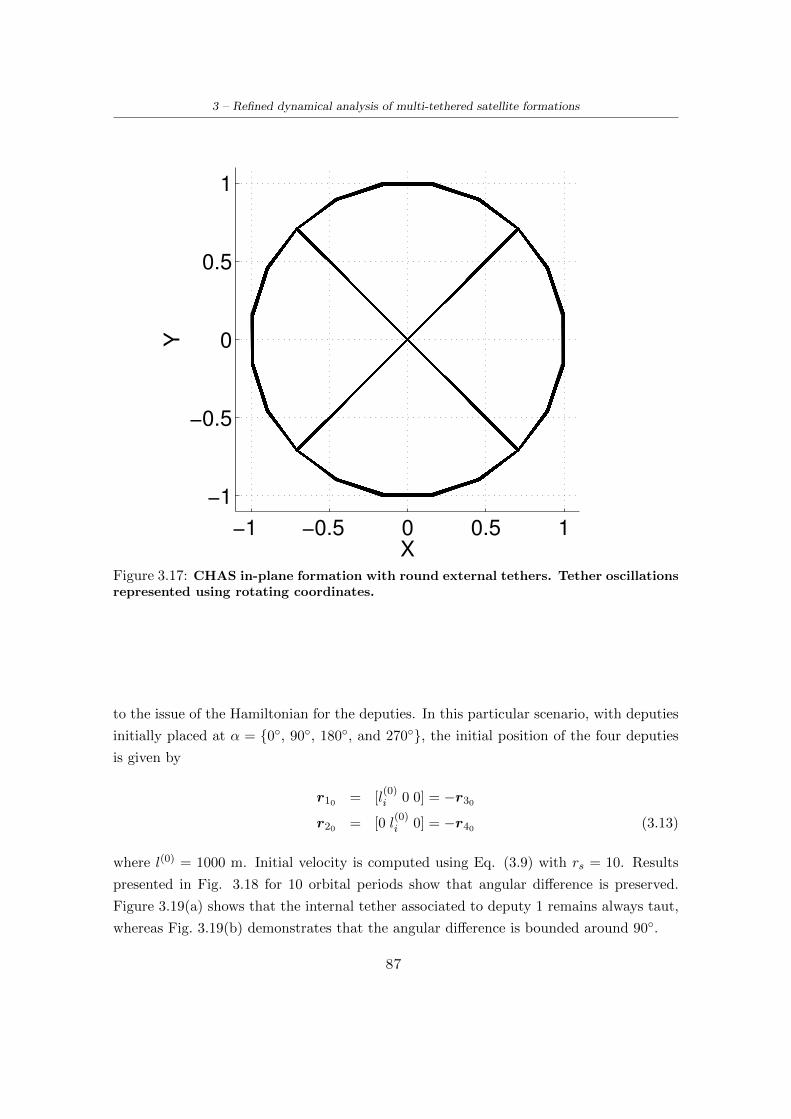
3 – Refined dynamical analysis of multi-tethered satellite formations
−1 −0.5 0 0.5 1
−1
−0.5
0
0.5
1
X
Y
Figure 3.17: CHAS in-plane formation with round external tethers. Tether oscillationsrepresented using rotating coordinates.
to the issue of the Hamiltonian for the deputies. In this particular scenario, with deputies
initially placed at α = 0, 90, 180, and 270, the initial position of the four deputies
is given by
r10 = [l(0)i 0 0] = −r30
r20 = [0 l(0)i 0] = −r40 (3.13)
where l(0) = 1000 m. Initial velocity is computed using Eq. (3.9) with rs = 10. Results
presented in Fig. 3.18 for 10 orbital periods show that angular difference is preserved.
Figure 3.19(a) shows that the internal tether associated to deputy 1 remains always taut,
whereas Fig. 3.19(b) demonstrates that the angular difference is bounded around 90.
87

3 – Refined dynamical analysis of multi-tethered satellite formations
−1 −0.5 0 0.5 1
−1
−0.5
0
0.5
1
X
Y
Figure 3.18: CHAS in-plane formation with round external tethers. Tether oscillationsrepresented using rotating coordinates.
3.4.2 Earth-facing formations
Using the initial conditions defined in Section 3.3.2, a simulation is performed using circu-
lar external tethers also for an Earth-facing formation. The behavior of the pitch angle δ
and the coplanarity measure (Fig. 3.20) show results similar to those presented in Fig. 3.10
for the corresponding CHAS Earth-facing formation with straight external tethers. As a
major difference, in this case internal tethers remain in tension and a regular behavior for
the position of the agents and of the parent body along the nominal orbit is obtained, as
shown in Fig. 3.21.
When one tries to stabilize the Earth-facing attitude by introducing anchors along the
radial direction, the bending of diagonal tethers connecting anchors to deputies cause the
anchors to move inwards, towards the parent body and this condition cannot be corrected
simply by making the diagonal tethers longer. The use of circular external tethers and
88
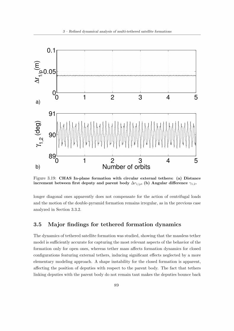
3 – Refined dynamical analysis of multi-tethered satellite formations
0 1 2 3 4 50
0.05
0.1
∆r 1
/p(m
)
0 1 2 3 4 589
90
91
γ 1,2
(d
eg
)
Number of orbitsb)
a)
Figure 3.19: CHAS In-plane formation with circular external tethers: (a) Distanceincrement between first deputy and parent body ∆r1/p, (b) Angular difference γ1,2.
longer diagonal ones apparently does not compensate for the action of centrifugal loads
and the motion of the double-pyramid formation remains irregular, as in the previous case
analyzed in Section 3.3.2.
3.5 Major findings for tethered formation dynamics
The dynamics of tethered satellite formation was studied, showing that the massless tether
model is sufficiently accurate for capturing the most relevant aspects of the behavior of the
formation only for open ones, whereas tether mass affects formation dynamics for closed
configurations featuring external tethers, inducing significant effects neglected by a more
elementary modeling approach. A shape instability for the closed formation is apparent,
affecting the position of deputies with respect to the parent body. The fact that tethers
linking deputies with the parent body do not remain taut makes the deputies bounce back
89

3 – Refined dynamical analysis of multi-tethered satellite formations
0 1 2 3 4−200
0
200
δ (
deg)
0 1 2 3 4−1
0
1
Copla
narity
Number of orbits
a)
b)
Figure 3.20: CHAS Earth-facing formation with circular external tethers: (a) Forma-tion orientation δ, (b) Coplanarity measure for deputies and parent body.
towards the parent body after full extension is reached. This instability is induced by the
variation in the shape of the external tethers and it cannot be predicted by means of the
simpler massless-cable model. In the case of the double-pyramid formation the instability
is even more serious, due to the fact that diagonal tethers connecting anchors to external
deputies experience the same centrifugal pull as the external tethers of closed formations,
but they are longer and more massive, thus inducing a more pronounced “bulging” effect
on the shape of the pyramid.
The behavior of the cluster as a whole, for open formations, is comparable to the one
predicted by the massless model with prescribed motion of the parent body. However in
closed formations, and more pronouncedly for the double-pyramid case, the parent body
of the formation does not remain on the reference orbit, as a consequence of the irregular
motion of agents, due to lack of tension in the internal tethers when external ones bend
90

3 – Refined dynamical analysis of multi-tethered satellite formations
0 1 2 3 4 5−0.02
0
0.02
0.04
∆r 1
/p(m
)
0 1 2 3 4 589
90
91
γ 1,2
(deg)
Number of orbits
a)
b)
Figure 3.21: CHAS Earth-facing formation with circular external tethers: (a) Distanceincrement between first deputy and parent body ∆r1/p, (b) Angular difference betweenadjacent tethers 1 and 2 (γ1,2).
under the action of centrifugal loads. This situation can be corrected for closed planar
formations by increasing the length of external tethers, in order to make them circular,
but the same strategy does not apply to the Double-Pyramid case.
91

Chapter 4
Multi-tethered formation
dynamics for non-ideal operating
conditions
In the previous chapter an ideal condition was assumed, when purely Keplerian motion was
considered and a reference circular orbit was selected. Orbit perturbations and a non-zero
value of the eccentricity for the whole orbit may lead to significant changes on tethered
formation dynamics, either when the formation is considered as a whole, or when the
relative position of each agent is considered. As an example, changes in the gravitational
force during an orbital period, lead to behavior non-observed in circular orbits as shown
in Ch. 2. At the same time, Table 2.1 lists the most significative perturbation in LEO is
due to variations in the Earth potential due the Earth oblateness. The present chapter is
focused on the effects of reference orbit eccentricity [135] and Earth’s oblateness [136] on
tethered formation dynamics.
4.1 Effects of eccentricity of the reference orbit on Multi–
Tethered Satellite Formations
When a non-circular reference orbit is considered, the dynamics of each agent of the multi-
tethered formation can be expressed by means of a model proposed in [17], where the
equations of relative motion for two spacecraft on neighboring elliptical orbits are derived
using time as independent variable (as shown in Equation 2.13), and then transformed
using true anomaly θ as the independent variable, in order to achieve a simpler compact,
92

4 – Multi-tethered formation dynamics for non-ideal operating conditions
periodic formulation. The transformation hinges on the chain rule for derivatives,
˙(·) = (·)′ θ ; (·) = (·)′′ θ2 + θ θ′(·)′ (4.1)
where a dot and a double dot indicate first and second derivatives with respect to
time t, respectively, whereas a prime and a double prime sign indicate first and second
derivatives with respect to θ.
For an object describing an elliptical orbit, the angular velocity depends on the true
anomaly. Letting e be the eccentricity of the orbit of the parent body and n the mean
motion, the local angular velocity of the orbiter along the reference orbit is given by [55]
θ =n(1 + e cos θ)2
(1− e2)3/2(4.2)
When the distance between the orbiting bodies remains small compared to the distance
of the origin O of the orbit frame from the center of the Earth, gravitational field can be
linearized around the current position of the centre of mass of the formation along the
reference orbit. The state vector for the i-th agent is given by its position and relative
position rates in the LVLH frame, that is, Xi = (xi′, xi, yi
′, yi, zi′, zi)
T . Note that position
rates with respect to true anomaly θ of the center of mass (indicated by primes) are used
instead of velocity components. The equations of motion for the i-th agent are expressed
by means of a periodic linear system in the form
dXi
dθ= [A(e, θ)] Xi + [B(n, e, θ)] f i/mi (4.3)
where the periodic matrices A and B are defined, respectively, as [17]
A=
2e sin θ
ζ
3 + e cos θ
ζ2
−2e sin θ
ζ0 0
1 0 0 0 0 0
−22e sin θ
ζ
2e sin θ
γ
e cos θ
ζ0 0
0 0 1 0 0 0
0 0 0 02e sin θ
ζ
−1
ζ0 0 0 0 1 0
93

4 – Multi-tethered formation dynamics for non-ideal operating conditions
and
B =(1− e2)3
ζ4n2
1 0 0
0 0 0
0 1 0
0 0 0
0 0 1
0 0 0
with ζ = (1+e cos θ). External forces and disturbances f i acting on the generic i-th agent
of the formation are also expressed in the LVLH frame, f i = fx,iiR+fy,ijR+fz,ikR, where
f i is the sum of external forces minus gravity (which is already accounted for) acting on
the i-th body of mass equal to mi.
4.1.1 Initial conditions for deputies and beads
Equation (4.3) is used to describe the motion of each deputy, bead and the parent body
of the formation. A set of initial conditions expressed in terms of position and velocity is
required for each one of these bodies, represented as a mass element. As mentioned above,
the independent variable is the true anomaly instead of time. For this reason, equations
are defined in terms of position rates and angular rates (with respect to θ) instead of
velocities. The geometry of the system is determined by the position of deputies ri in the
LVLH frame and how connecting tethers are arranged. First of all, the initial conditions
on position and position rates need to be defined for parent body and deputies. The initial
conditions for the beads are then derived from the former ones.
The initial condition for the velocity components of the parent body is computed using
the expression that ensures that the orbit of the parent does not present any secular drift
with respect to the center of mass of the formation. This constraint is enforced by assuming
that when the cluster is initialized at perigee (θ = 0) the following relation holds [17]
y′p0xp0
= −[
2 + e
1 + e
](4.4)
Following the approach described in [13], the formation spins around an axis perpen-
dicular to the formation plane, in the attempt of gyroscopically stabilizing them. This
angular rate induces a relative motion of each deputy with respect to the parent body.
94

4 – Multi-tethered formation dynamics for non-ideal operating conditions
Assuming that (i) the parent is placed in the origin of the LVLH frame, and (ii) the ve-
locity of formation elements at the initial time t = 0 follows that of a rigid body, with an
angular velocity equal to ω0, the position rate of deputy d is given by
r′d0 = r′p0 + ω0 × rd0 (4.5)
where r′p0 = x′p0 iR + y′p0 jR + z′p0 kR is the initial position rate of the parent, defined
above, ω0 = ω0/θ is the angular rate of the formation relative to the orbit frame, and rd0is the initial relative position vector of the deputy, where all the vectors are expressed in
terms of components in the LVLH frame.
For in-plane formations, it is possible to define a local non dimensional spin rate,
ωd/p = ωd/p/θ (4.6)
that provides a measure of the spin speed of deputy d around the parent, scaled with
respect to the time derivative of the true anomaly. This scalar parameter is equal to
ωd/p = ‖(r′d − r′p)− (r′d − r′p) · id/p‖/‖rd − rp‖ (4.7)
where id/p = (rd − rp)/‖rd − rp‖ is the unit vector parallel to the relative position of
the deputy with respect to the parent body. The initial angular position for the deputies
is chosen such that a constant angular separation is maintained when ωd/p = ‖ω0‖ is
assumed at the initial time, t = 0 [13]. Equation (4.7) requires that agents and parent
body constantly lie on the same plane. When the initial spin plane of the formation is
not maintained during the evolution, as it happens with Earth-facing formations, Equa-
tion (4.7) does not hold.
Given the initial position for the deputies, tether configuration, and number nt of beads
in tether t, it is possible to derive the position of the bead labelled b at the initial time
assuming that they are equally spaced,
rb0 = rd/p0 + (rd?0 − rd/p0)(1− jt/nt) , jt = 1, 2, . . . , nt (4.8)
where the tether is assumed to connect a generic deputy d? placed in rd?0 to either another
deputy d or the parent body p in rd/p0 . The initial position rate for each bead follows the
same assumption of relative motion used in the case of the deputies, that is, a rigid-body
95

4 – Multi-tethered formation dynamics for non-ideal operating conditions
velocity distribution expressed by Eq. (4.5), such that
r′b0 = r′p0 + ω0 × rb0 (4.9)
The approach used to define the characteristics of the orbit scenarios considered in
this study takes into account that the cluster is initialized at the perigee. Therefore, when
defining the initial conditions of the agents, it is necessary to define the value of ω0 at
θ = 0. There are different possible criteria to define the size and shape of the orbits of the
cluster through the semimajor axis a and eccentricity e. In this study a constant perigee
radius is assumed equal to Rp = 6578 km for all the reference orbits, which corresponds
to an approximate altitude of 200 km over the Earth surface and it is equal to the radius
of the circular reference orbit considered in Ref. [13].
The distance R between the primary body (the Earth, in the present case) and the
center of mass of the formation is expressed in polar coordinates as [55]
R(θ) =a(1− e2)1 + e cos θ
(4.10)
For given values of eccentricity e and perigee altitude Rp, the semimajor axis a is given
by a = Rc/(1 − e). The mean motion for the considered orbit is n =√µ/a3, where µ is
Earth’s gravitational parameter. Note that it is not possible to consider orbits with the
same mean motion n (that is, the same semi-major axis), because perigee altitude would
go below Earth’s radius for small values of the eccentricity, resulting into unfeasible orbits
crossing the Earth’s surface. The semi-major axis for the reference orbit needs thus to be
increased when cases with e > 0 are to be dealt with and perigee altitude is prescribed.
Defining the same value of ω0 for all the scenarios considered having different eccen-
tricities is not considered a viable option, as the approach used to define the reference
orbit for each value of e leads to orbits with different mean motion and orbital periods.
Sizeable differences in the dimensional values of formation angular speed would be ob-
tained for different cases, that in turn cause different tensions in the tether system and
centrifugal loads. Considering that all the scenarios have the same perigee altitude, which
is equal to the altitude of reference circular orbit, the value of ω0 is chosen such that the
clusters flying different orbits are characterizes by the same dimensional angular velocity
at perigee pass, a value which will be indicated as
ω0P = rs · nc h (4.11)
96

4 – Multi-tethered formation dynamics for non-ideal operating conditions
Table 4.1: Orbit and agents characteristics
Parameter Symbol Value Units
Perigee altitude Rp 6578 km
Eccentricity values e 0.0, 0.3, 0.5
Mass of parent body 300 kg
Mass of deputies body 25 kg
The initial angular velocity of the formation is thus defined as a factor rs of the circular
orbit mean motion nc having a perigee radius Rc = Rp = 6578 km. The direction of the
initial formation angular rate, h, depends on the particular scenario (either Earth-facing,
with h = iR, or in-plane formations, with h = kR). Using the transformation defined in
Eq. (4.1), the initial value of the angular rate ω0 at perigee is equal to
ω0 =ω0P
θ(θ=0)
=
(rs√1 + e
)h (4.12)
4.1.2 Formation stability
Provided that the major objective of this work is to evaluate the effect of eccentricity and
tether mass on the dynamics of tethered satellite formations, the behavior of each con-
figuration considered in this study is compared with the behavior of the same formations
when tethers are modeled as massless elastic cables, for different values of the eccentricity
of the cluster orbit. The tether characteristics is the same as the one defined in Chapter
3, in Table 3.2, and also in accordance with [13].
The stability of the cluster is analyzed performing a numerical simulation of the dy-
namic model. Similar to the work performed in Chapter 3, in order to assess stability of
the formation the following features are observed in the simulations.
In-plane formations
The initial condition for the position of the four deputies of the formation is set to
r10 = [l(0)i l
(0)i 0] ·
√2/2 = −r30
r20 = [−l(0)i l(0)i 0] ·
√2/2 = −r40 (4.13)
97

4 – Multi-tethered formation dynamics for non-ideal operating conditions
where l(0) = 1000 m. In Ref. [13], a method for calculating initial velocities of the deputies
is proposed, which is based on the calculation of the Hamiltonian for each tether initial
orientation, in order to ensure that tethers exhibit the same trajectory without presenting
any drift in their relative position. This approach is specific for circular reference orbits,
but when used for formations of four deputies on elliptical orbits, it provides again an ini-
tial relative position such that the angular separation between deputies remains constant.
It can be shown that, in order to ensure a constant angular difference, it is sufficient to
initially place the four deputies at angles α1 = 45, α2 = 135, α3 = 225 and α4 = 315
with respect to the iR axis, and use the same initial value of spin rate ωi/p = ‖ω0‖ for all
four deputies.
Initial position rate at perigee is computed using Eq. (4.5), with the parent body placed
in the origin of the orbit frame and
ω0 =[0 0 rs/
√1 + e
](4.14)
In the case of a HAS in-plane formation, a value of rs = 10 is selected for all deputies. For
the CHAS in-plane formation, it is rs = 15, for consistency with Ref. [13]. Simulations
are run considering three different values of eccentricity: e = 0.0 (circular orbits), e = 0.3
and e = 0.5.
For in-plane formations, due to the fact that there is no net gravity gradient torque on
the satellite, it is possible to invoke conservation of angular momentum. The dissipation
caused by damping in the tethers is assumed negligible. In addition to the considerations
relative to Thomson equilibria for rigid bodies, outlined in 2, the model considered in
this paper, based on discrete point masses, clearly shows that in-plane and transverse
dynamics are uncoupled, when initial position and velocities lie on the orbit plane. This
means, again, that a planar spinning formation lying initially on the orbital plane will
evolve on this plane.
Hub-and-spoke in-plane formation
In this section, the results for deputies 1 and 2, of a HAS in-plane formation are discussed.
The behavior of deputies 3 and 4 is perfectly equivalent, and it will not be presented.
Figures 4.1 to 4.3 show the dynamic behavior in terms of deputy position, local spin rate
98
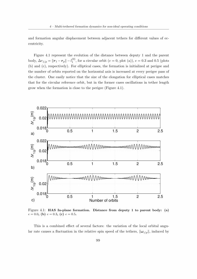
4 – Multi-tethered formation dynamics for non-ideal operating conditions
and formation angular displacement between adjacent tethers for different values of ec-
centricity.
Figure 4.1 represent the evolution of the distance between deputy 1 and the parent
body, ∆r1/p = ‖r1− rp‖− l(0)1 , for a circular orbit (e = 0, plot (a)), e = 0.3 and 0.5 (plots
(b) and (c), respectively). For elliptical cases, the formation is initialized at perigee and
the number of orbits reported on the horizontal axis is increased at every perigee pass of
the cluster. One easily notice that the size of the elongation for elliptical cases matches
that for the circular reference orbit, but in the former cases oscillations in tether length
grow when the formation is close to the perigee (Figure 4.1).
0 0.5 1 1.5 2 2.50.018
0.02
0.022
∆r 1
/p(m
)
0 0.5 1 1.5 2 2.50.018
0.02
0.022
∆r 1
/p(m
)
0 0.5 1 1.5 2 2.50.018
0.02
∆r 1
/p(m
)
Number of orbits
a)
c)
b)
Figure 4.1: HAS In-plane formation. Distance from deputy 1 to parent body: (a)e = 0.0, (b) e = 0.3, (c) e = 0.5.
This is a combined effect of several factors: the variation of the local orbital angu-
lar rate causes a fluctuation in the relative spin speed of the tethers, ‖ωi/p‖, induced by
99

4 – Multi-tethered formation dynamics for non-ideal operating conditions
conservation of absolute angular momentum, such that if the formation spins at an ap-
proximately constant angular speed with respect to the inertial frame (as in the present
case), its angular speed relative to the LVLH orbit frame becomes smaller at perigee, when
orbit rate is higher, and vice-versa it is higher at apogee, when the orbit rate is lower (Fig-
ure 4.2, upper plot). This effect is amplified when θ is used as the independent variable. In
this case the non-dimensional relative angular rate, ω1/p = ω1/p/θ, is obtained by dividing
the dimensional value by the local orbit rate which is higher at the perigee.
At the same time, the gravity gradient forcing term is more intense closer to the Earth
and this causes a stronger periodic action on tethers while the formation spins at a slower
rate at perigee pass, relative to the orbit frame. On the other hand, when the formation
moves away from perigee and the influence of the gravity field becomes weaker, oscillations
almost vanish in amplitude, but they are characterized by a higher frequency, related to
the more frequent passage of each deputy along the local vertical, when the formation an-
gular speed relative to the LVLH frame grows. This effect increases with orbit eccentricity,
when the distance from the cluster to the Earth at apogee is higher, if a constant perigee
altitude is assumed, as in the present case.
When transforming the nondimensional spin rate of deputy 1, ω1/p, defined accord-
ing to Eq. (4.7), into its dimensional counterpart, ω1/p = ω1/pθ (shown in Fig. 4.2(b)),
an increase in the spin rate close to apogee is still visible, which is due to conservation
of angular momentum around the orbit normal, but this effect is clearly less relevant in
quantitative terms, with variations in the order of 5 up to 7% of the initial formation
angular rate. This means that variations in amplitude of the oscillations is mostly related
to variations of orbit rate θ and intensity of gravity gradient between their maximum and
minimum values at perigee and apogee, respectively.
Higher frequency terms in the variation of angular velocity shown in the bottom plot
of Fig. 4.2(b) are related to the exchange between kinetic and potential energy due to the
orientation of the deputy (deputy 1 in the considered example) in the LVLH frame. This
can be proven taking into account the expressions of kinetic and potential energy derived
in [13] and the fact that the total energy is conserved. In this respect dissipative damp-
ing forces in the tethers can be neglected, as they depend on elongation rate only, which
is small, thus producing only a negligible effect on the short term evolution of total energy.
100
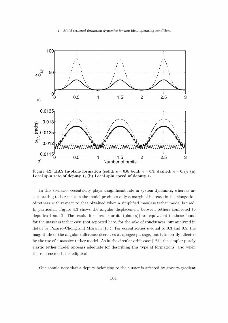
4 – Multi-tethered formation dynamics for non-ideal operating conditions
0 0.5 1 1.5 2 2.5 30
50
100
ω1/p
0 0.5 1 1.5 2 2.5 30.0115
0.012
0.0125
0.013
0.0135
Number of orbits
ω1/p
(ra
d/s
)
a)
b)
Figure 4.2: HAS In-plane formation (solid: e = 0.0; bold: e = 0.3; dashed: e = 0.5): (a)Local spin rate of deputy 1, (b) Local spin speed of deputy 1.
In this scenario, eccentricity plays a significant role in system dynamics, whereas in-
corporating tether mass in the model produces only a marginal increase in the elongation
of tethers with respect to that obtained when a simplified massless tether model is used.
In particular, Figure 4.3 shows the angular displacement between tethers connected to
deputies 1 and 2. The results for circular orbits (plot (a)) are equivalent to those found
for the massless tether case (not reported here, for the sake of conciseness, but analyzed in
detail by Pizarro-Chong and Misra in [13]). For eccentricities e equal to 0.3 and 0.5, the
magnitude of the angular difference decreases at apogee passage, but it is hardly affected
by the use of a massive tether model. As in the circular orbit case [121], the simpler purely
elastic tether model appears adequate for describing this type of formations, also when
the reference orbit is elliptical.
One should note that a deputy belonging to the cluster is affected by gravity-gradient
101

4 – Multi-tethered formation dynamics for non-ideal operating conditions
0 0.2 0.4 0.6 0.8 190
90.5
91
γ1,2
(d
eg
)
0 0.5 1 1.5 2 2.5 3 3.5 490
90.5
91
γ1,2
(d
eg
)
0 0.5 1 1.5 2 2.5 3 3.5 490
90.5
91
γ1,2
(d
eg
)
Number of orbits
a)
b)
c)
Figure 4.3: HAS In-plane formation. Angular distance between deputies 2 and 1: (a)e = 0.0, (b) e = 0.3, (c) e = 0.5.
force on two different timescales. On one side, the spin rate of a deputy derived from
Eq. (4.7), is not constant, and it oscillates with its angular position, as already demon-
strated in Ref. [13], where a Hamiltonian for the system is formulated that allows for
computing initial conditions of different deputies with equal energy values for avoiding
secular variations in their relative angular position. On the other hand, the angular rate
of the whole cluster varies with true anomaly for elliptical orbits, as discussed above and
shown in Figure 4.2. The superposition of these two motions is highlighted in Figure 4.4(a),
shows the spin rates relative to the parent body, ω1/p and ω2/p, of deputies 1 and 2, respec-
tively. The enlargement highlights the difference in agent spin rates associated to different
orientations within the cluster at perigee pass, where this effect is more significant. Plot
(b) shows the evolution of ω2/p− ω1/p over two orbits, which explains the variation in the
angular displacement γ1,2 between tethers connected to the considered deputies shown in
Figure 4.3.
102

4 – Multi-tethered formation dynamics for non-ideal operating conditions
0 0.5 1 1.5 20
50
100ω
i/p
0 0.5 1 1.5 2−0.2
−0.1
0
0.1
0.2
ω2/p
−ω
1/p
Number of orbits
a)
b)
Figure 4.4: HAS In-plane formation: (a) Spin rate for agents 1 (solid) and 2 (dashed),(b) Spin rate difference between agents 1 and 2.
0 0.5 1 1.5 2−2
−1
0
1
2x 10
−4
ω2/p
−ω
1/p
(ra
d/s
)
Number of orbital periodsFigure 4.5: HAS In-plane formation: Dimensional spin rate difference between agents1 and 2 as a function of time, t/TO.
The increase in frequency of the oscillations at apogee visible in the lower plot of Fig-
ure 4.4 is only apparent, as it is mostly related to the use of true anomaly as independent
variable, as in [17]. The actual frequency of the oscillations in the time domain can be
103

4 – Multi-tethered formation dynamics for non-ideal operating conditions
easily recovered by plotting ω2/p−ω1/p as a function of time, where t = t(θ, e) is obtained
from Kepler’s time equation [55]. The frequency of the oscillations of ω2/p − ω1/p as a
function of time is almost constant (Figure 4.5), whereas the amplitude of the oscillations
of this dimensional variable undergoes more severe variations over one orbit, when com-
pared to its non-dimensional counterpart.
Closed hub-and-spoke in-plane formation
The closed in-plane formation presents the same initial relative position of deputies with
respect to the parent adopted for the open formation, with the relevant difference rep-
resented by the presence of external tethers connecting deputies (as shown in Fig. 3.1).
In order to properly analyze the shape of the formation, a rotating coordinate reference
system is introduced. The rotating reference, formed by unit vectors iS , jS , and kR, is
chosen such that its angular velocity around the normal to the orbit plane kR is equal
to the average spin rate of internal tethers relative to the orbit frame. This allows for
removing the overall formation rotation dynamics and to highlight deviations from a nom-
inal, ideal behavior of uniform spin speed for all the agents. The behavior of deputies,
beads and tethers and their relative oscillations from the ideal in-plane rotation can thus
be determined. Initial position and velocity for the four deputies is set following the pro-
cedure already summarized in the previous section for the HAS in-plane case, so that all
the agents and tethers have the same spin rate at initial time.
The results for a simulation of 4 orbital periods are presented in Figs. 4.6 and 4.7 for
e = 0.0 and e = 0.3 respectively. Variables X and Y are the position variables in the
iS − jS plane scaled with respect to l(0). The shape of the formation is characterized by
two effects. First of all, external tethers are subject to a centrifugal pull that bends them,
transforming the initial square into a “rounded” quadrangle. This fact, in turn, affects the
relative position of deputies with respect to the parent body as the direction of external
tether tension acting on the deputies is varied with respect to the nominal square shape
and the tension force on the internal tethers vanishes, as long as they do not reach full
extension. This represents a major difference with respect to the massless tether model,
already discussed in Ch. 3.
The effects of eccentricity on formation geometry is only apparently marginal, as there
are at least two significant differences between the cases of circular and elliptical reference
104

4 – Multi-tethered formation dynamics for non-ideal operating conditions
-0.8 -0.6 -0.4 -0.2 0 0.2 0.4 0.6 0.8
-0.8
-0.6
-0.4
-0.2
0
0.2
0.4
0.6
0.8
X
Y
Figure 4.6: CHAS In-plane formation. Shape of formation (6-orbit run), e = 0.0
orbits. For e = 0 the external tethers approach the bulged configuration almost monoton-
ically, residual vibrations being present which are related only to the loads transmitted by
internal tethers during the rotation when one or more of them reaches full extension. On
the converse, the oscillations in formation rotation rate induced by the periodic variation
of orbit rate coupled with differences in gravity gradient intensity at perigee and apogee
(as discussed above) force vibrations in the external tethers during the whole time-history.
At the same time, the behaviour of the oscillations for internal tethers appears to be less
regular for e = 0.3, with oscillations that are characterized by different amplitude and
frequency between different tethers and for the same tethers during different orbits.
This latter fact is confirmed by the analysis of Figs. 4.8 and 4.9, where the evolution
of ∆ri/p = ‖ri − rp‖−l(0)i (when tethers are taut ∆ri/p = ∆li) is presented for e = 0.0 and
e = 0.3 respectively. In both cases, three out of four deputies are close to full extension
at the same time, whereas the fourth one, connected to an agent that reduces its distance
105

4 – Multi-tethered formation dynamics for non-ideal operating conditions
-0.8 -0.6 -0.4 -0.2 0 0.2 0.4 0.6 0.8
-0.8
-0.6
-0.4
-0.2
0
0.2
0.4
0.6
0.8
X
Y
Figure 4.7: CHAS In-plane formation. Shape of formation (10-orbit run), e = 0.3.
from the parent body by approximately 16 m, remains loose. In the circular case the
slack tether changes constantly, whereas, in the elliptical orbit case, one of the tethers
remains loose for long time intervals (up to several revolutions). Changes between loose
and (almost) taut conditions usually take place at or close to perigee pass, where the effect
of the gravity gradient is stronger and differences on the gravity pull acting on different
deputies get higher.
The result is that for the circular case, short-term fluctuations of ∆ri/p are highly
irregular for all the agents of the formation, but they are characterized by high-frequency
variations of the distance between each deputy and parent body with similar characteris-
tics. On the converse, high-frequency variations of ∆ri/p almost disappear in the elliptic
case, when one of the tethers remains loose for long time intervals, allowing for wider fluc-
tuations of beads under the action of gravity gradient only, with no tension acting between
106

4 – Multi-tethered formation dynamics for non-ideal operating conditions
0 1 2 3 4 5 6−20
0
20
∆r 1
/p(m
)
0 1 2 3 4 5 6−20
0
20
∆r 2
/p(m
)
0 1 2 3 4 5 6−20
0
20
∆r 3
/p(m
)
0 1 2 3 4 5 6−20
0
20
∆r 4
/p(m
)
Number of orbits
a)
b)
c)
d)
Figure 4.8: CHAS In-plane formation. Distance ∆ri/p time evolution, e = 0.0.
them in the loose tether. This can also be seen in Figure 4.9, where the internal tether
linking deputy 2 shows smaller oscillations, after an initial transient, due to the fact that
it never becomes slack. When eccentricity is increased, this behavior is more pronounced,
and for e = 0.7 the same tether remains slack for a simulation of 10 orbits.
When compared to the open formation in-plane case, external tethers in closed forma-
tions provide a stabilizing effect for the angular displacement of adjacent tethers. Even at
high values of eccentricity (e = 0.7), the angular displacement between adjacent tethers
remains close to 90. As discussed in Paragraph 4.1.2 the rounded shape induced by the
centrifugal pull can be compensated either by making external tethers lext longer, or re-
ducing the internal tether length, lint, such that the ratio between their lengths becomes
lext/lint <√
2. This avoids or at least limits the irregular fluctuations in the distance
between deputies and parent body.
107

4 – Multi-tethered formation dynamics for non-ideal operating conditions
0 1 2 3 4 5 6 7 8 9 10−20
0
20
∆r 1
/p(m
)
0 1 2 3 4 5 6 7 8 9 10−20
0
20
∆r 2
/p(m
)
0 1 2 3 4 5 6 7 8 9 10−20
0
20
∆r 3
/p(m
)
0 1 2 3 4 5 6 7 8 9 10−20
0
20
∆r 4
/p(m
)
Number of orbits
b)
a)
c)
d)
Figure 4.9: CHAS In-plane formation. Distance ∆ri/p time evolution, e = 0.3.
Earth-facing formations
The initial condition for the position of the four deputies of the formation for the Earth-
facing case is set to
r10 = [0 l(0)i l
(0)i ] ·
√2/2 = −r30
r20 = [0 − l(0)i l(0)i ] ·
√2/2 = −r40 (4.15)
Initial velocity is computed using Equation (4.5) with the parent body placed at the
origin of the LVLH frame and
ωi/p =
[− rs√
1 + e0 0
](4.16)
where l(0) = 1000 m. The value of rs is set to rs = 10 for both open HAS and CHAS
Earth-facing formations, as in [13]. The initial condition of beads is computed following
the same procedure as for the in-plane formation.
108

4 – Multi-tethered formation dynamics for non-ideal operating conditions
For an Earth-facing formation, deputies and tethers initially lie on the horizontal jR-
kR plane of the LVLH orbital reference frame. The fact that initial values of zi and
corresponding velocity components are non-zero leads to tridimensional trajectories, in
contrast to what happens for the in-plane case, where initial conditions and resulting tra-
jectories remain constrained on the iR-jR orbit plane.
In the Earth-facing scenario, it is no longer possible to establish an analogy with the
attitude behavior of a spinning rigid body, as transverse dynamics becomes relevant and
deputies no longer lie on the same plane, normal to the formation spin axis, especially
when spin rates are in the same order of magnitude as the orbit mean motion. For the
specific case of a spin axis pointing along the Nadir direction, a null spin rate relative to
the orbit frame is required. Such a situation is clearly not realistic for a tethered forma-
tion, as in this case tethers loose tension, the formation does not maintain its shape, and
the analogy with a rigid body is not valid anymore.
Therefore, for a circular orbit it is not possible to achieve a relative equilibrium state
in which the spin axis of the formation points along the radial axis iR in the LVLH frame.
For elliptical orbits, Likins-Pringle equilibria do not exist at all, and it is not possible to
achieve any relative equilibrium state in which the formation constantly faces the Earth.
As opposite to the in-plane case, the net torque exerted by the gravity gradient on an
Earth-facing formation is not null in general, and therefore it is no longer possible to invoke
conservation of angular momentum. Reference [122] provides a detailed study on the
variation of the angular momentum vector of a spinning satellite under the gravitational
field. But in all the cases here considered formations are provided with a spin rate sufficient
for gyroscopically stiffening the tethers. Thanks to this rotation rate, angular momentum
is high, and fluctuations of angular momentum induced by gravity gradient over one orbit
remain sufficiently small.
Hub-and-spoke Earth-facing formation
Coupling between orbital plane dynamics and crossrange dynamics peculiar to this sce-
nario makes the orientation between the formation plane and the radial axis not constant.
Provided that gravity torque affects only marginally the direction of angular momentum,
the spin axis of the formation and the direction of angular momentum point approximately
109

4 – Multi-tethered formation dynamics for non-ideal operating conditions
along an inertially fixed direction. Therefore, the component of angular momentum in the
radial direction at initial time remains almost constant, and agents of the formation rotate
(approximately) on an inertially fixed plane that spins around the orbit normal with re-
spect to the orbit frame. This means that the formation is not constantly facing the Earth.
This fact is confirmed by the angle δ, measured between the radial axis iR and the
vector n normal to the plane defined by the deputies and parent body. The angle δ, shown
in Figure 4.10, grows monotonically between −180 and 180. The angle is assumed 0 at
perigee and it switches from -180 and 180 at apogee, making the formation unstable
from the point of view of the desired Earth-pointing attitude of the formation. The same
figure also shows that in this respect the effect of eccentricity on δ is not relevant. As it can
be observed, the variation of the pitch angle for e = 0.5 (plot (b)) follows almost exactly
the same pattern of the circular case (plot (a)). Only small amplitude higher frequency
fluctuations of δ are affected by e, as oscillations become less frequent when the formation
gets closer to perigee pass. This effect is similar to that observed for angular displacement
in open in-plane formations (Figure 4.3), and it is related to the same causes, but it is less
relevant from the point of view of the application.
The pattern of the elongation of tethers for open formations differs significantly from
that observed for the in-plane configuration. Again, highly eccentric reference orbits cause
the gravity gradient to become weaker when the cluster moves away from perigee, but this
time a reduction of the amplitude of oscillations is observed for higher values of e and
the amplitude of oscillations almost vanish at both apogee and perigee passes (that is
N = 0.5, 1.0, 1.5 and 2 orbits), when the formation lies on a plane perpendicular to
the radial direction. This is shown in Figure 4.11, where oscillations in tether length are
represented. This figure also shows that massless and massive tether models result into
a dynamic behaviour qualitatively very similar, where the only (and hardly noticeable)
effect is a slightly higher elongation ∆li for the massive tether case.
Also the angular distance between adjacent tethers oscillates according to a pattern
that depends on eccentricity in all cases, as shown in Figure 4.12. This represents a behav-
ior peculiar of this type of configuration that could not be found for the in-plane formation
case, when oscillations in the angular displacement almost disappear at apogee. Again, no
significant differences can be observed when comparing the massive and massless models,
which is a characteristic already found for in-plane open formations.
110

4 – Multi-tethered formation dynamics for non-ideal operating conditions
0 1 2 3 4−200
0
200
δ (
deg)
0 1 2 3 4−200
0
200
δ (
deg)
Number of orbits
a)
b)
Figure 4.10: HAS Earth-facing formation pitch angle δ. (a) e = 0.0, (b) e = 0.5.
Closed hub-and-spoke Earth-facing formation
The initial condition for agents and beads belonging to internal and external tethers are
defined as for the in-plane case, but placed in an Earth-facing orientation in this scenario.
As for the HAS case, the deputies approximately lie on a plane that performs a complete
rotation around the axis kR during each orbit around the primary body (Figure 4.13). In
addition to this, external tethers present the same deformation induced by the centrifugal
load that can be observed for closed in-plane formations. Consequences for internal tethers
are similar, with at least one internal tether loosing tension, all of them vibrating in the
transverse direction. Oscillations and variations of distance between formation agents are
qualitatively similar to those observed in the CHAS in-plane scenario and are not reported
for the sake of conciseness.
111

4 – Multi-tethered formation dynamics for non-ideal operating conditions
0 0.5 1 1.5 20.015
0.016
0.017
∆r 1
/p(m
)
0 0.5 1 1.5 20.015
0.016
0.017
∆r 1
/p(m
)
0 0.5 1 1.5 20.015
0.016
0.017
Number of orbits
∆r 1
/p(m
)
b)
c)
a)
Figure 4.11: HAS Earth-facing formation distance ∆r1/p. Solid: massive model,dashed: massless model. (a) e = 0.0, (b) e = 0.3, (c) e = 0.5.
4.1.3 Behavior of the parent body
The analysis of the dynamic behavior of the formation is completed by inspecting the tra-
jectory followed by the parent body of the formation. In all the configurations presented
in this paper, the position of the parent body at initial time coincides with that of the
center of mass of the formation, which is the origin of the LVLH reference frame. For this
reason, as discussed previously (see in particular Eq. (4.4)), the initial condition of the
parent is determined in order to avoid secular drift of the cluster away from the reference
orbit. Consequently, the initial velocity of the parent is set to zero along the axes iR, jR,
and kR of the LVLH frame. Figure 4.14 shows the distance between the reference elliptical
orbit and the parent body for different configurations and eccentricity e equal to 0 (solid
lines) and 0.5 (dashed ones). The distance Dp = ‖rp‖ is given by the norm of the position
of the parent body in the LVLH frame.
In the case of open formations, the position of the parent body remains almost exactly
112

4 – Multi-tethered formation dynamics for non-ideal operating conditions
0 0.2 0.4 0.6 0.8 189
90
91
γ1,2
(d
eg
)
0 0.5 1 1.5 2 2.5 389
90
91
γ1,2
(d
eg
)
0 0.5 1 1.5 2 2.5 389
90
91
γ1,2
(d
eg
)
Number of orbits
b)
a)
c)
Figure 4.12: HAS Earth-facing formation, angle γ1,2. (a) e = 0.0, (b) e = 0.3, (c) e = 0.5.
on the reference orbit. Dp grows in time, but in the order of 10−9 m, clearly related more
to numerical errors when integrating the equations of motion then to some physical effects.
In these two cases the position of the center of mass coincides with that of the parent body
for the whole simulation.
On the other hand, for closed formations the evolution of the position of the parent
body exhibits a different behavior. For both in-plane and Earth-facing cases, the center
of mass remains on the reference orbit as in open formations, which demonstrates how
numerical errors in the integration do not cause violation of this important physical fact.
However, the position of the parent body does not remain on the reference elliptical orbit
described by the center of mass of the formation. The distance Dp remains bounded, but it
presents considerable aperiodic fluctuation. In the case of in-plane formations, the parent
body shows a motion that can be approximately confined to a circle with a 2 m radius
around the reference orbit, as presented in Figure 4.15, so that stability of the formation
is not compromised. Wider deviations are present for the Earth-facing case, with peak
113
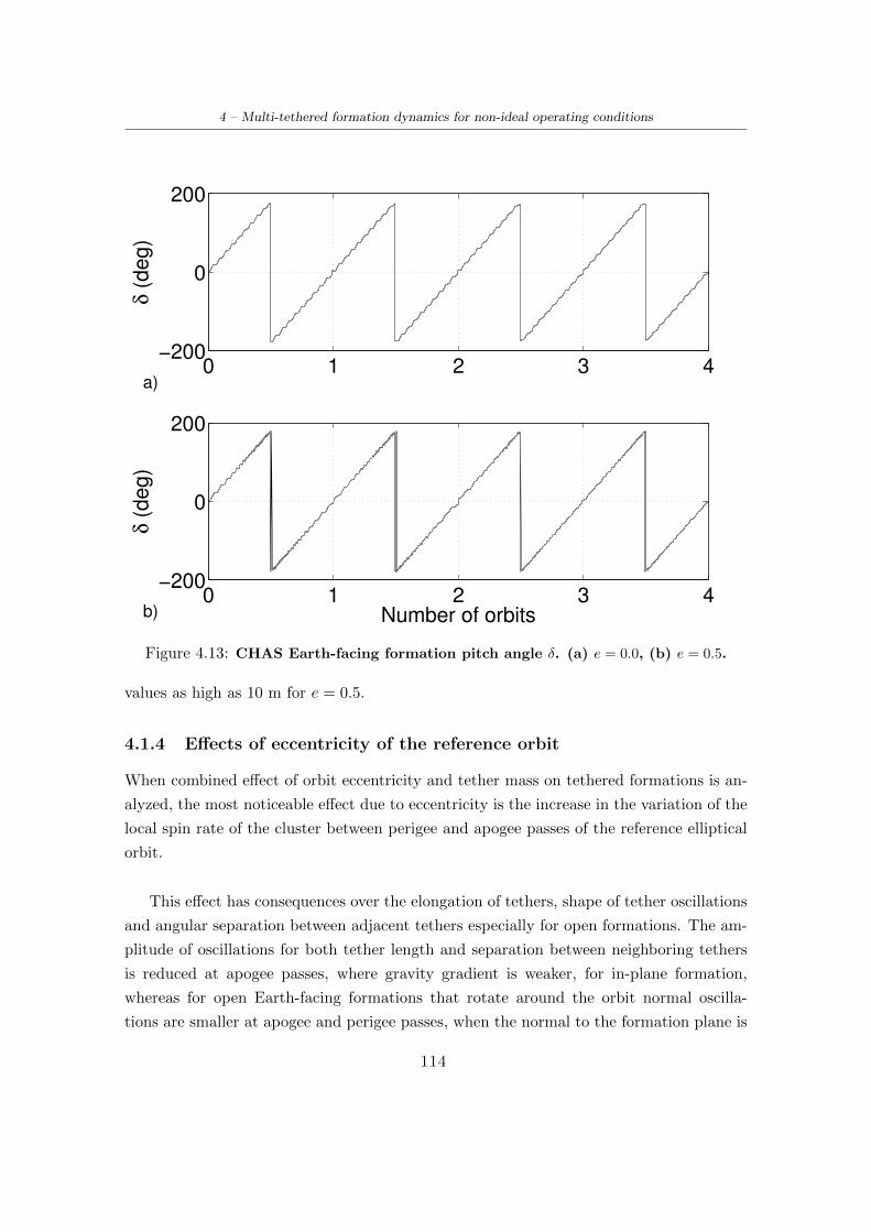
4 – Multi-tethered formation dynamics for non-ideal operating conditions
0 1 2 3 4−200
0
200
δ (
deg)
0 1 2 3 4−200
0
200
δ (
deg)
Number of orbitsb)
a)
Figure 4.13: CHAS Earth-facing formation pitch angle δ. (a) e = 0.0, (b) e = 0.5.
values as high as 10 m for e = 0.5.
4.1.4 Effects of eccentricity of the reference orbit
When combined effect of orbit eccentricity and tether mass on tethered formations is an-
alyzed, the most noticeable effect due to eccentricity is the increase in the variation of the
local spin rate of the cluster between perigee and apogee passes of the reference elliptical
orbit.
This effect has consequences over the elongation of tethers, shape of tether oscillations
and angular separation between adjacent tethers especially for open formations. The am-
plitude of oscillations for both tether length and separation between neighboring tethers
is reduced at apogee passes, where gravity gradient is weaker, for in-plane formation,
whereas for open Earth-facing formations that rotate around the orbit normal oscilla-
tions are smaller at apogee and perigee passes, when the normal to the formation plane is
114

4 – Multi-tethered formation dynamics for non-ideal operating conditions
0 0.5 1 1.5 2 2.5 3 3.5 40
2
4x 10
−9
Dp (
m)
0 0.5 1 1.5 2 2.5 3 3.5 40
5x 10
−9
Dp (
m)
0 0.5 1 1.5 2 2.5 3 3.5 40
2
4
Dp (
m)
0 0.5 1 1.5 2 2.5 3 3.5 40
10
20
Dp (
m)
Number of orbits
a)
b)
c)
d)
Figure 4.14: Distance Dp. (a) HAS In-plane, (b) HAS Earth-facing, (c) CHAS In-plane, (d) CHAS Earth-facing. Solid, e = 0.0, dashed, e = 0.5
aligned with the radial direction (with maxima when the formation is in quadrature with
the primary body). These effects are more noticeable as eccentricity of the reference orbit
is increased.
For closed formations external tethers provide a stabilizing effect on angular separation
between adjacent tethers. On the other hand, centriphugal loads bend external tethers,
preventing deputies from achieving a stable position because the tethers that connect them
with the parent body are not in tension. For eccentric orbits, as the cluster moves away
from perigee and the gravity gradient becomes weaker, the formation shows a more stable
behavior, where a single tether remains loose for long time intervals, in contrast with the
circular orbit case, when the slack tether changes continuously. These effects cannot be
observed when the simulation model does not feature a massive tether model, as tether
mass plays a crucial role in the dynamics of the system.
115

4 – Multi-tethered formation dynamics for non-ideal operating conditions
−3 −2 −1 0 1 2 3−3
−2
−1
0
1
2
3
X (m)
Y (
m)
Figure 4.15: Trajectory of parent body of CHAS In-plane formation for e = 0.7 (6orbits).
4.2 Effects of J2 perturbation on tethered formations
The combined effects of tether mass (simulated by means of a discrete bead model [14])
and J2 perturbation on the dynamics of various tethered formations is now analyzed tak-
ing into account the dynamics modeled in Eqs. 2.33 and 2.34.
4.2.1 Initial conditions for deputies and beads
Equations 2.33 and 2.34 are used to describe the motion of each deputy, bead and the
parent body of the formation. An initial condition in terms of position and velocity is
needed for each one of these bodies, represented as a mass element. The initial condition
for velocity of the parent body is computed using the expressions presented in Ref. [16]
that ensures that the orbit of the parent does not present any secular drift. These initial
conditions are on xp0 and yp0 , and depend on the initial values, xp0 and yp0 , for the same
116
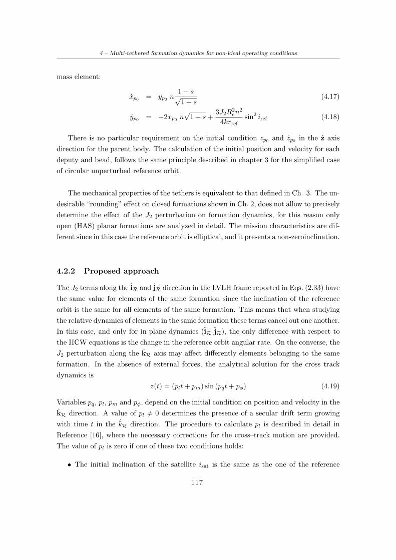
4 – Multi-tethered formation dynamics for non-ideal operating conditions
mass element:
xp0 = yp0 n1− s√1 + s
(4.17)
yp0 = −2xp0 n√
1 + s+3J2R
2en
2
4krrefsin2 iref (4.18)
There is no particular requirement on the initial condition zp0 and zp0 in the z axis
direction for the parent body. The calculation of the initial position and velocity for each
deputy and bead, follows the same principle described in chapter 3 for the simplified case
of circular unperturbed reference orbit.
The mechanical properties of the tethers is equivalent to that defined in Ch. 3. The un-
desirable “rounding” effect on closed formations shown in Ch. 2, does not allow to precisely
determine the effect of the J2 perturbation on formation dynamics, for this reason only
open (HAS) planar formations are analyzed in detail. The mission characteristics are dif-
ferent since in this case the reference orbit is elliptical, and it presents a non-zeroinclination.
4.2.2 Proposed approach
The J2 terms along the iR and jR direction in the LVLH frame reported in Eqs. (2.33) have
the same value for elements of the same formation since the inclination of the reference
orbit is the same for all elements of the same formation. This means that when studying
the relative dynamics of elements in the same formation these terms cancel out one another.
In this case, and only for in-plane dynamics (iR-jR), the only difference with respect to
the HCW equations is the change in the reference orbit angular rate. On the converse, the
J2 perturbation along the kR axis may affect differently elements belonging to the same
formation. In the absence of external forces, the analytical solution for the cross track
dynamics is
z(t) = (plt+ pm) sin (pqt+ pφ) (4.19)
Variables pq, pl, pm and pφ, depend on the initial condition on position and velocity in the
kR direction. A value of pl /= 0 determines the presence of a secular drift term growing
with time t in the kR direction. The procedure to calculate pl is described in detail in
Reference [16], where the necessary corrections for the cross–track motion are provided.
The value of pl is zero if one of these two conditions holds:
• The initial inclination of the satellite isat is the same as the one of the reference
117

4 – Multi-tethered formation dynamics for non-ideal operating conditions
orbit;
• The initial separation in the longitude of the ascending node between the satellite
and the reference orbit ∆Ω0 is zero.
Values for isat and ∆Ω0 can be calculated from the following equations:
isat = z0/(krref) + iref
∆Ω0 = arcsin
[sin(z0/rref)
sin(iref)
]≈ z0rref sin(iref)
(4.20)
In conclusion, the presence of secular motion for a particular body in the formation is
determined by the initial condition on z0 and z0. Depending on the structure and orien-
tation of the formation, it is possible to fulfill at least one of these two conditions. For
in–plane formations deputies and tethers lie on the same reference orbit plane, such that
both conditions, z0 = z0 = 0 are satisfied. Therefore the absence of any secular drifting
motion is guaranteed.
The case of Earth–facing configurations is more complex. For the elements lying on
the iR-jR plane at initial time, the z0 = 0 condition is satisfied, whereas for elements with
z0 /= 0, the requirement for the absence of secular behaviour is satisfied only if the relative
motion at initial time provides a zero value for the initial speed component normal to the
orbit plane, that is, z0 = 0. In the most general case a secular term is present, that affects
the resulting behaviour of the formation.
As anticipated above, the behaviour of Hub–And–Spoke (HAS) and Closed–Hub–And–
Spoke (CHAS) formations for in–Plane and Earth–Facing configurations is analysed in the
sequel.
4.2.3 Open–loop dynamics of tethered formation
The purpose of this chapter is to evaluate the effect of the J2 perturbation on tethered
satellite formations. For this reason, the behaviour of a HAS formation will be compared
with the behaviour of the same formation in the absence of the perturbation. The scenario
incorporating the perturbation is that of a non–equatorial orbit, since it is the case where
the perturbation effect is more significant. The inclination of the orbit is iref = 45 and
the altitude of the parent body is 200 Km above the surface of the Earth. The effects of
the perturbation on formations flying in equatorial orbits are much less significative than
118

4 – Multi-tethered formation dynamics for non-ideal operating conditions
in non-equatorial orbits and are not considered in the sequel. The stability of the cluster
is analyzed by performing a numerical simulation of the dynamic model as in Ch. 2.
In-plane formations
For the HAS in–plane formation, all the deputies plus the parent body lie in the orbital
plane. Since equations for orbital dynamics and cross–track dynamics are uncoupled, the
fact that z0 = 0 and z0 = 0 eliminates any cross–track trajectory. This configuration
simplifies considerably the equations, since isat = iref and ∆Ω0 = 0. The absence of
cross-track motion in the in–plane formation, makes the correction in the reference orbital
rate the only change in the equations of motion with respect to the unperturbed equation
model, because as outlined above the J2 term in the iR and jR direction is the same for
all elements of the cluster.
The position initial condition for the four deputies of the formation is set to:
r10 = [l(0)i l
(0)i 0] ·
√2/2 = −r30
r20 = [−l(0)i l(0)i 0] ·
√2/2 = −r40 (4.21)
Initial velocity is computed using Equation (3.2) with the parent object placed at the
origin of the LVLH frame and
ω0 = [0 0 rsω] (4.22)
where l(0) = 1000 m and ω = nc. In the case of the HAS in–plane formation, the value of
rs is set to rs = 10. The initial condition of beads is computed in the same way, with the
local angular velocity equal to that of the deputy belonging to each tether.
The results shown in Fig. 4.16 demonstrate that values for tether elongation are very
close, when comparing the unperturbed case with that in the presence of J2 effects. The
figure represents the increment of the distance between the first deputy and the parent
body, but the behaviour is rather similar also for the other three deputies. Only a slight
phase shift in the oscillations and a minimal change in distance increment can be noticed.
These minor variations are due to the fact that the orbital rate with the J2 model is slightly
faster, and this has an impact over the initial velocity of deputies that are computed as a
factor of ω. The orbital angular velocity n is increased by a factor c = 1.00019.
As far as the angular distance between tethers is concerned, in the absence of the J2
119

4 – Multi-tethered formation dynamics for non-ideal operating conditions
0 0.05 0.1 0.15 0.20
0.01
0.02
0.03
∆r 1
/p(m
)
12.8 12.85 12.9 12.95 130.0195
0.02
0.0205
∆r 1
/p(m
)
Number of orbits
b)
a)
Figure 4.16: HAS in–plane formation. Distance increment between first deputy andparent body ∆l1, (solid line, with J2 effects; dotted one, without J2).
perturbation the angle between tethers connecting adjacent deputies oscillates around 90
with an amplitude of less than 0.5 and a mean value slowly increasing with time. In
Fig. 4.17 it can be appreciated how in the perturbed scenario (plot (b)), the increase of
mean value of the oscillations grows faster than in the non–perturbed case (plot (a)). This
fact affects formation stability, where in spite of the elongation of the tethers being fairly
stable, with the formation keeping its orientation within the orbital plane, the angular
displacement between pairs of tethers slowly grows, thus making in the long run two of
the tethers fold onto the neighbouring ones.
Earth-facing formations
Earth–facing configurations exhibit a more complex behaviour than in–plane formations
due to the presence of cross–track dynamics. First of all, even though the deputies of an
Earth–facing formation initially lie on the jR− kR plane and have an initial velocity with
non–zero components along one or both these axes, with initial values in the iR direction
x0 = 0 and x0 = 0, the dynamic equations clearly show that values of y0 /= 0 or y0 /= 0
120

4 – Multi-tethered formation dynamics for non-ideal operating conditions
0 2 4 6 889.5
90
90.5
γ1,2
(deg)
0 2 4 6 889.5
90
90.5
91
γ1,2
(deg)
− J
2
Number of orbitsb)
a)
Figure 4.17: HAS in–plane formation. Angular separation between tethers 1 and 2,γ1,2 without J2 effects (a) and with J2 (b).
affect the dynamics in the iR direction as well, thus creating a three-dimensional trajec-
tory. Incorporating tethers creates an additional coupling due to the constraint imposed
by tether length: tension forces exchanged between pairs of bodies directly connected by
a tether couple cross–track and and in–plane dynamics.
The initial condition for the position of the four deputies of the formation is set to
r10 = [0 l(0) l(0)] ·√
2/2 = −r30 (4.23)
r20 = [0 − l(0) l(0)] ·√
2/2 = −r40
whereas initial velocity is computed according to Eq. (3.2) with the parent object placed
at the origin of the LVLH frame and
ωi/p = [−rsω 0 0] (4.24)
121

4 – Multi-tethered formation dynamics for non-ideal operating conditions
A value of l(0) = 1000 m is again chosen for the nominal length of tethers connecting the
parent body to the deputies. As for the angular speed, it is ω = nc with values of rs set to
rs = 10 for all deputies and tethers, as indicated in Ref. [13] for the massless tether case.
The value of rs is the same for the HAS and CHAS formation scenarios.
Note that the considered initial condition provides for a situation where none of the
deputies satisfy one of the conditions necessary for making the secular drift term to vanish,
that is, either z0 = 0 or z0 = 0. The l term of the cross–track dynamics affects all the
deputies (and most of the beads), and therefore, all these masses should present a secular
drift, which is counteracted upon by the presence of tether tension.
In terms of distance between external agents and parent body, the behaviour (pre-
sented in Fig. 4.18) is similar to that observed for the in–plane formation considered in
the previous subsection. As for the angular displacement, in this case, there is almost no
difference between the perturbed and unperturbed scenarios, as demonstrated by the plots
in Fig. 4.19. As for the elongation, minor differences are present, due to the different or-
bital rate used to compute the velocity initial condition of deputies, as required in Eq. (3.2).
The overall behaviour of the formation is the same observed for the unperturbed sce-
nario in a way similar to what happens for the massless tether case). Figure 4.20 shows how
the normal vector to the formation, tilts around the x axis, and that the four deputies
plus the parent body are coplanar most of the time. The coplanarity parameter C, as
defined in Eq. (3.7) is reported in Fig. 4.20(b).
4.2.4 Effect of the J2 perturbation on the parent body
As described previously, the equations of motion take into consideration the fact that the
parent body is not attached to the reference orbit. In an unperturbed scenario, the centre
of mass of the formation always remains on the reference orbit, with small oscillations
of the parent body around the reference due to internal forces exerted by tethers. How-
ever, when J2 perturbation affects deputies and beads in a different way, small variations
of tether tension may results that are not perfectly balanced on the parent body, thus
pulling it away, in the long run, from the reference orbit. As a consequence, the whole
formation slowly drifts away from the reference orbit.
In Fig. 4.21, the distance Dp between the parent and the reference orbit is computed
for the different scenarios studied in this study. As it can be seen, in–plane orbits are less
122
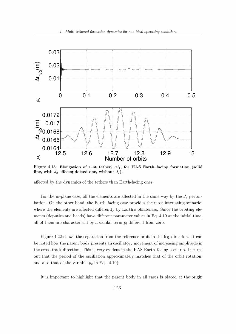
4 – Multi-tethered formation dynamics for non-ideal operating conditions
0 0.1 0.2 0.3 0.4 0.5
0.01
0.02
0.03
∆r 1
/p(m
)
12.5 12.6 12.7 12.8 12.9 130.0164
0.0166
0.0168
0.017
0.0172
∆r 1
/p(m
)
Number of orbits
a)
b)
Figure 4.18: Elongation of 1–st tether, ∆l1, for HAS Earth–facing formation (solidline, with J2 effects; dotted one, without J2).
affected by the dynamics of the tethers than Earth-facing ones.
For the in-plane case, all the elements are affected in the same way by the J2 pertur-
bation. On the other hand, the Earth–facing case provides the most interesting scenario,
where the elements are affected differently by Earth’s oblateness. Since the orbiting ele-
ments (deputies and beads) have different parameter values in Eq. 4.19 at the initial time,
all of them are characterized by a secular term pl different from zero.
Figure 4.22 shows the separation from the reference orbit in the kR direction. It can
be noted how the parent body presents an oscillatory movement of increasing amplitude in
the cross-track direction. This is very evident in the HAS Earth–facing scenario. It turns
out that the period of the oscillation approximately matches that of the orbit rotation,
and also that of the variable pq in Eq. (4.19).
It is important to highlight that the parent body in all cases is placed at the origin
123

4 – Multi-tethered formation dynamics for non-ideal operating conditions
0 2 4 6 889
89.5
90
90.5
γ1,2
(deg)
12 12.1 12.2 12.3 12.4 12.589.2
89.4
89.6
89.8
90
90.2
γ1,2
(deg)
Number of orbits
a)
b)
Figure 4.19: Angular separation between tethers 1 and 2, γ1,2 (solid line, with J2effects; dotted one, without J2).
with zero velocity. This initial condition should make the parent body to lie on the orbit
plane. However, the forces exerted by tethers with non-zero secular terms (Earth-facing
scenarios) move it apart from the reference orbit with oscillations of growing amplitude.
The same Earth-facing configurations without the J2 perturbation show the behaviour
presented in Fig. 4.23, where it can be clearly seen that a bounded oscillation in the kR
direction is present with respect to the reference orbit.
4.2.5 Effects of J2 perturbation on formation behavior
This study has presented the effects of incorporating the J2 effect on massive tethered
satellite formations modelled following a HCW approach. No significant differences were
found in terms of elongation of tethers and angular separation for the HAS and CHAS
configurations in the in-plane and Earth-facing orientations. In the Earth–facing scenario,
124

4 – Multi-tethered formation dynamics for non-ideal operating conditions
0 5 10 150
90
180
δ (
deg
)
0 5 10 15−1
0
1
Cop
lan
arity
Number of orbits
a)
b)
Figure 4.20: Orientation and coplanarity parameters for the HAS Earth–facing forma-tion.
objects of the formation are affected differently by the perturbation, some of them poten-
tially having secular drifts. It is interesting to observe that the trajectory of the parent
body in the Earth–facing cases presents oscillations of increasing amplitude in the kR
(cross–track) direction. As it was pointed before, in this case, all the elements of the
formation are affected differently by the perturbation in their cross–track dynamics.
125

4 – Multi-tethered formation dynamics for non-ideal operating conditions
0 5 10 150
0.5
1
1.5x 10
−3
Dp (
m)
HAS In−plane
Orbits0 5 10 15
0
0.5
1
1.5
Dp (
m)
HAS Earth−facing
Orbits
0 5 10 150
1
2
3
Dp (
m)
CHAS In−plane
Orbits0 5 10 15
0
5
10
15
Dp (
m)
CHAS Earth−facing
Orbitsc)
a) b)
d)
Figure 4.21: Distance of parent body from reference orbit.
126

4 – Multi-tethered formation dynamics for non-ideal operating conditions
0 5 10 15−1
−0.5
0
0.5
1
Z (
m)
HAS In−plane
Orbits0 5 10 15
−2
−1
0
1
2
Z (
m)
HAS Earth−facing
Orbits
0 5 10 15−1
−0.5
0
0.5
1
Z (
m)
CHAS In−plane
Orbits0 5 10 15
−4
−2
0
2
4
Z (
m)
CHAS Earth−facing
Orbits
a) b)
c) d)
Figure 4.22: Elevation along the Z axis of parent body.
127

4 – Multi-tethered formation dynamics for non-ideal operating conditions
0 5 10 15−1
−0.5
0
0.5
1x 10
−4
Z (
m)
HAS Earth−facing (non J2)
Orbits
0 5 10 15−4
−2
0
2
4
Z (
m)
CHAS Earth−facing (non J2)
Orbits
a)
b)
Figure 4.23: Elevation in Z axis of parent (no J2)
128

Chapter 5
Tethered Formation Control
The behavior of tethered formations in Low Earth Orbit was analyzed in Ch. 3 and 4
proving that there is no formation configuration that guarantees a stable natural equilib-
rium of a spinning tethered cluster. Only formations lying in the orbital plane present a
certain degree of stability, but still a controller is needed to ensure that deputies maintain
the desired position. This chapter presents a control strategy for a tethered formation
cluster that provides position and attitude control.
Taking into account the arguments presented in Ch. 2, the Thomson and the coni-
cal Likins–Pringle equilibrium orientations appear as the most appropriate for practical
purposes. The latter, in particular, allows for an almost Earth–facing orientation when a
small tilt angle γ is achieved. The cluster geometry chosen for this study is the Double–
Pyramid without parent body, since according to [76] exhibits a behavior similar to that
of a spinning rigid body.
5.1 Formation Flying Control
One of the reasons to study the behavior and control tethered formations is to address
ultimately the formation flying problem. Reference [137] provides a deep insight into
spacecraft formation flying topics. As cited in this book, formation flying is about “The
tracking or maintentance of a desired spacecraft separation, orientation or position be-
tween or among spacecrafts”. References [138] and [139] summarize a state of the art
of Spacecraft Formation Flying. The first paper addresses the guidance problem, which
consist in defining the appropriate relative orbits, whereas the second is focused on active
129

5 – Tethered Formation Control
control strategies. Reference [140] studies the stability of the relative motion dynamics of
two spacecraft in the phase plane taking into account the J2 perturbation. Decentralized
control techniques applied to satellite flight formation are explored in references [22] and
[141]. Other modern control techniques like optimal control, adaptive control and µ con-
trol are studied in references [108], [142], [143] and [144] respectively.
5.2 Tethered Formation Flying Control
Figure 5.1 shows a diagram of the most common mission profiles related to tether forma-
tions. The nomenclature follows that used in references [1] and [138]. Relative orbits can
be passive (PRO) or active (ARO). In the first case, no active control is needed, whereas in
the second case a control loop needs to be implemented to maintain the relative configura-
tion of formation members. In Deep Space (DS) applications, relative spacecraft dynamics
in general is not subject to orbital dynamics or external perturbations, which is the case
of Planet Orbital Environment (POE) missions. The POE literature is focused mainly on
finding Passive Relative Orbits (PRO). The case of Active Relative Orbits (ARO) is that
case requiring closed loop control to maintain the structure within the required configu-
ration shape.
Figure 5.1: Mission Profiles (taken from [1] and [138])
Among Tethered (PRO) formations there are dynamic formations where the struc-
ture is stabilized through centrifugal and in some cases gravitational forces. Gravitational
130

5 – Tethered Formation Control
forces have a stabilizing role for Earth-pointing dumbell tethers as described in detail in
Ch. 2, due to differential gravity effect on tether ends.
The static formations PROs, can be stabilized through drag, by the gravitational po-
tential, or electromagnetically. On a tethered system moving through the Earth’s magnetic
field, electric potential is created along conductive tethers. This fact can be used to gen-
erate electrical power/thrust as presented in [1].
When implementing an active controller, solving the spacecraft formation flying control
problem can be further decomposed in two different problems, or a combination of both:
• Development of control strategies allowing for the reconfiguration of the formation
(e.g. expansion, contraction or change of orientation of the whole set of agents). This
involves developing techniques to avoid spacecraft interference and collision. This is
a coarse control strategy with the purpose of orientating the overall formation along
an specific direction. This kind of control is specially suited for missions in which
the overall cluster must point to a specific direction.
• Development of control laws aimed at maintaining the relative position with respect
to an inertially fixed attitude along the orbit (inertial station keeping). Accurate
precision control requires compensating perturbations. This level consist of a fine
control approach in order that each agent achieves the desired location and orien-
tation with respect to a formation-fixed reference frame, assuming 6-DOF agent
control capability.
5.3 Virtual Structure Control Approach
This section introduces the virtual structure control approach, both in the centralized and
decentralized versions. This technique will be adapted for formation control of a tethered
formation.
5.3.1 Centralized Virtual Structure Control Approach
In addition to frames O (inertial) and R (LVLH) introduced in Chapter 2, two additional
reference frames are needed to define the virtual structure approach. Frame F is fixed
at the center of the formation (or equivalently the center of the virtual structure); frame
I is a reference frame fixed at agent i. Following the same approach proposed in Ref-
erence [20], the equations of motion for the translational and rotational dynamics of the
131

5 – Tethered Formation Control
virtual structure are given by
rF
MF vF˙qF˙qF
JF ωF
λF
λF
=
vF
fF
−12ωF × qF + 1
2 qFωF
−12ωF · qF
−ωF × JFωF + τF
λF
σF
(5.1)
The state variables of this equation are the rigid body position vector rF , the velocity
vector, vF , the rigid body attitude quaternion qF = (qF , qF ), the body angular velocity
ωF , and the two vectors of parameters λF and µF . Parameters λF and µF are used to
express the expansion ratio and expansion rate of the formation along the axes of F . The
position and orientation of the virtual structure F is controlled through the main controls
of force fF , torque τF , and straint σF for controlling position, attitude and expansion
ratio respectively. Constants MF and JF are the virtual mass and inertia tensors of the
virtual structure F . Reference [20] presents a control law that stabilizes the virtual struc-
ture to a given position, attitude and expansion ratio.
The state of the formation is defined by the coordination vector,
ξF = [rTF ,vTF , q
TF ,ω
TF ,λ
TF , λ
TF ]T (5.2)
which provides the state of the virtual structure F , and consequently the overall shape
of the formation. In the centralized approach, this vector is broadcasted to all the agents
of the formation and each agent derives its own desired state to be tracked in order to
maintain the formation shape.
The desired position and orientation of the i–th agent with respect to the virtual struc-
ture is defined through vector XdiF = [rdiF ,v
diF , q
diF ,ω
diF ] which expresses the desired state
of the agent i in the F reference frame. If the shape of formation must remain fixed, the
components of XiF will be constant.
Letting the direction cosine matrix CRF be the transformation from the virtual struc-
ture based reference frame F to the orbit frame R, the following equations transform
132
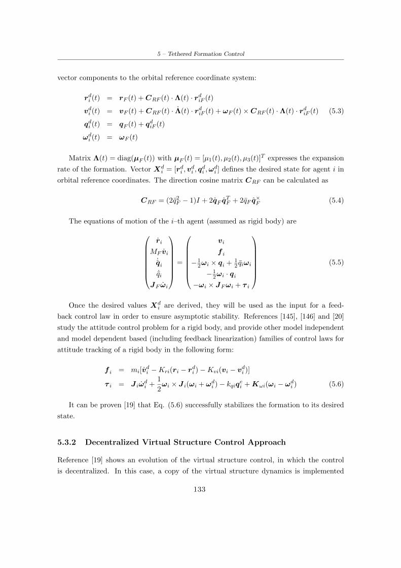
5 – Tethered Formation Control
vector components to the orbital reference coordinate system:
rdi (t) = rF (t) +CRF (t) ·Λ(t) · rdiF (t)
vdi (t) = vF (t) +CRF (t) · Λ(t) · rdiF (t) + ωF (t)×CRF (t) ·Λ(t) · rdiF (t) (5.3)
qdi (t) = qF (t) + qdiF (t)
ωdi (t) = ωF (t)
Matrix Λ(t) = diag(µF (t)) with µF (t) = [µ1(t), µ2(t), µ3(t)]T expresses the expansion
rate of the formation. Vector Xdi = [rdi ,v
di , q
di ,ω
di ] defines the desired state for agent i in
orbital reference coordinates. The direction cosine matrix CRF can be calculated as
CRF = (2q2F − 1)I + 2qF qTF + 2qF q
×F (5.4)
The equations of motion of the i–th agent (assumed as rigid body) areri
MF vi˙qi˙qi
JF ωi
=
vi
f i
−12ωi × qi + 1
2 qiωi
−12ωi · qi
−ωi × JFωi + τ i
(5.5)
Once the desired values Xdi are derived, they will be used as the input for a feed-
back control law in order to ensure asymptotic stability. References [145], [146] and [20]
study the attitude control problem for a rigid body, and provide other model independent
and model dependent based (including feedback linearization) families of control laws for
attitude tracking of a rigid body in the following form:
f i = mi[vdi −Kri(ri − rdi )−Kvi(vi − vdi )]
τ i = J iωdi +
1
2ωi × J i(ωi + ωdi )− kqiqei +Kωi(ωi − ωdi ) (5.6)
It can be proven [19] that Eq. (5.6) successfully stabilizes the formation to its desired
state.
5.3.2 Decentralized Virtual Structure Control Approach
Reference [19] shows an evolution of the virtual structure control, in which the control
is decentralized. In this case, a copy of the virtual structure dynamics is implemented
133

5 – Tethered Formation Control
on each satellite, producing a local coordination vector i that evolves under the feedback
obtained from the adjacent neighbors in the formation. In this approach, an instance
of the virtual structure is integrated on each deputy. Differences between the state of
adjacent virtual structure instances are corrected by using appropriate control terms. The
equations of motion of each virtual structure Fi are
rFi
MF vFi˙qFi˙qFi
JFiωFi
λFi
λFi
=
vFi
fFi
−12ωFi × qFi + 1
2 qFiωFi
−12ωFi · qFi
−ωFi × JFωFi + τFi
λFi
σFi
(5.7)
The transformation to the desired values is performed using again Eq. (5.3), but in this
case, the calculation of CRFi is based on the individual instantiation of the orientation
quaternion qFi rather than qF used in the centralized case. Position, orientation and
expansion ratio of each virtual structure Fi are controlled through the main controls of
force fFi, torque τFi, and straint σFi for changing position, attitude and expansion ratio
respectively. The coordination vector in this case is specific for each instance ξFi instead
of a global coordination vector ξFi. Reference [19] proposes the control law
fFi =MF −KG(rFi − rdF )− ΓGivFi+
−KS(rFi − rF (i+1))−DS(vFi − vF (i+1))+
−KS(rFi − rF (i−1))−DS(vFi − vF (i−1))
τFi =− kG qd∗F qFi − ΓGiωFi+
− kS q∗F (i+1)q∗F (i) −DS [ωFi − ωF (i+1)]+ (5.8)
− kS q∗F (i−1)q∗F (i) −DS [ωFi − ωF (i−1)]
σFi =−KGqd∗F qFi − ΓGiωFi+
− ΓS [λFi − λF (i+1)]−DS [µFi − µF (i+1)]+
− ΓS [λFi − λF (i−1)]−DS [µFi − µF (i−1)]
ΓGi = DG +KF · eT i = DG +KF ‖Xi‖2
The term ΓGi provides the formation feedback [21] from low level (agent level) control
134
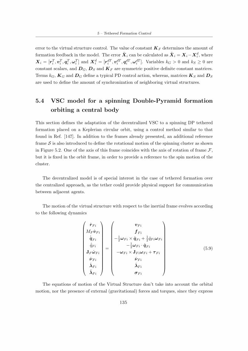
5 – Tethered Formation Control
error to the virtual structure control. The value of constant KF determines the amount of
formation feedback in the model. The error Xi can be calculated as Xi = Xi−Xdi , where
Xi = [rTi ,vTi , q
Ti ,ω
Ti ] and Xd
i = [rdTi ,vdTi , qdTi ,ωdTi ]. Variables kG > 0 and kS ≥ 0 are
constant scalars, and DG, DS and KF are symmetric positive definite constant matrices.
Terms kG, KG and DG define a typical PD control action, whereas, matrices KS and DS
are used to define the amount of synchronization of neighboring virtual structures.
5.4 VSC model for a spinning Double-Pyramid formation
orbiting a central body
This section defines the adaptation of the decentralized VSC to a spinning DP tethered
formation placed on a Keplerian circular orbit, using a control method similar to that
found in Ref. [147]. In addition to the frames already presented, an additional reference
frame S is also introduced to define the rotational motion of the spinning cluster as shown
in Figure 5.2. One of the axis of this frame coincides with the axis of rotation of frame F ,
but it is fixed in the orbit frame, in order to provide a reference to the spin motion of the
cluster.
The decentralized model is of special interest in the case of tethered formation over
the centralized approach, as the tether could provide physical support for communication
between adjacent agents.
The motion of the virtual structure with respect to the inertial frame evolves according
to the following dynamics
rFi
MF vFi˙qFi˙qFi
JF ωFi
νFi
λFi
λFi
=
vFi
fFi
−12ωFi × qFi + 1
2 qFiωFi
−12ωFi · qFi
−ωFi × JFiωFi + τFi
νFi
λFi
σFi
(5.9)
The equations of motion of the Virtual Structure don’t take into account the orbital
motion, nor the presence of external (gravitational) forces and torques, since they express
135

5 – Tethered Formation Control
Figure 5.2: Orbiting spinning double pyramid cluster. Reference frames
the ideal motion of an spinning rigid body to be matched by the cluster. If the virtual
structure is required to remain fixed on the circular orbit, then r = 0 and v = 0. The
expansion dynamics defined by variable λ is used to model tether extension through a
deployment/retrieval mechanism. Variable νFi defines the spin velocity of the formation,
and νFi the angle between frames S and F .
The simple translational agent dynamics of Equation (5.5) for ri is now substituted
by HCW equations xi − 2nyi − 3n2xi
yi + 2nxi
zi + n2zi
=f imi
(5.10)
which model the dynamics of agents in the R frame coordinates, taking into account the
effect of the gravity gradient. The angular rate n = (µ/R3)1/2 describes the rotation rate
of reference frame R with respect to the inertial frame O, where µ = GM⊕ is Earth’s
gravitational parameter and R is the radius of the considered circular orbit.
136

5 – Tethered Formation Control
In Equation (5.10), force f i = fi,x, fi,y, fi,z is the resultant of external forces acting
on agent i. It is the sum of the control force and forces exerted by tethers f i = ui,control +
f i,tens. The approach to calculate elastic force is presented in Eq.(2.41) in the tether
elasticity model section 2.4.1. The control force is supposed to track a desired position
Xdi and velocity X
di profiles.
The rotational dynamics of i–th agent,
˙qi˙qi
JF ωi
=
−12ωi × qi + 1
2 qiωi
−12ωi · qi
−ωFai × JFωi + τ g,i + τ c,i
(5.11)
where τ g,i = −3n2 · (kO × JF · kO) is the gravity gradient torque (defined as in [67]) and
τ c,i is the control torque. The rotation rate of frame F with respect to the inertial frame
O, is expressed as ωFai = ωF + n · kO.
The calculation of the desired state Xdi = [rdi ,v
di , q
di ,ω
di ] for each deputy, follows a
similar principle to the one defined in the section describing the general virtual structure
approach. As shown in Reference [20], the virtual structure approach allows to set the
orientation of the whole cluster and define a quaternion feedback control law to success-
fully point the structure along a required direction. However, in the case of a spinning
formation it is not only needed to control the orientation of the formation, but it is also
needed to keep it spinning along the commanded axis. For this purpose, an additional
rotation matrix CFiSi that relates frames F and S, is introduced in the calculation of the
agent desired position and velocity. This rotation matrix will depend on the angle νFi
and the vector φ that defines the direction of νFi (the spinning motion of the rigid body),
which will be typically one of the axis of the reference frame F .
The expansion parameter Λ typically used to stretch the formation is included in this
case to control the reeling of the tethers attached to the two anchors. This allows to
change the inertia properties of the cluster.
137

5 – Tethered Formation Control
The desired position and velocity of each agent is expressed as
rdi (t) = rFi(t) +CRFi(t) ·CFiSi(t) ·Λ(t) · rdiF (t)
vdi (t) = vFi(t) + (CRFi(t) ·CFiSi(t) · Λ(t) +
ωFi(t)×CRFi(t) ·CFiSi(t) ·Λ(t) +
CRFi(t) · (νFi · φ×CFiSi(t)) ·Λ(t)) · rdiF (t) (5.12)
qdi (t) = qFi(t) + qdiF (t)
ωdi (t) = ωFi(t)
where the term
CRFi = (2q2Fi − 1)I + 2qFiqTFi + 2qFiq
×Fi (5.13)
represents the direction cosine matrix used to transform vector components from the frame
F which defines the axis of the pointing vector of the virtual structure, to the desired to
the LVLH frame coordinates. In this equation, the position rdiF defines indeed the position
of a deputy in frame S. Therefore, a constant value of rdiF means that in fact the deputy
will be spinning with frame S with respect to frame F .
Reference [19] includes a convergence analysis that proves position and velocity Lya-
punov asymptotic stability. The proof is based on the construction of Lyapunov function
based on four terms:
V = Vsp + VFt + VFr + VFe (5.14)
where the term Vsp = Vsp(ri, vi, qi, ωi) includes the state variables related to the po-
sition and orientation of each agent, and the rest of the terms VFt = VFt(rFi,vFi),
VFr = VFt(qFi,ωFi), and VFe = VFe(λFi, λFi) include the state variables related to
the decentralized virtual structure dynamics. The reference first proves that V ≤ 0 and
subsequently by using LaSalle’s invariance principle the stability proof is extended to
prove asymptotic stability. For the tethered formation equations of motion terms describ-
ing the virtual structure coordination remain the same in this approach, and therefore
the same logic can be applied to ensure that the decentralized coordination approach is
asymptotically stable. On the other hand, the term Vsp that includes the i-th agent state
variables has a different expression as the agent state is affected by tether tension and
gravitational forces. The following section proposes a control approach to ensure stability
of Xi = [rTi , vTi , q
Ti , ω
Ti ].
138

5 – Tethered Formation Control
5.5 Fine positioning control
The Virtual Structure Control approach defines formation control at two levels. At the
outer level, the overall formation control sets attitude and position of the overall formation
(the virtual structure). At the inner one, the fine precision control regulates position and
attitude of the formation members with respect to the virtual structure fixed reference
frame. Provided that a satisfactory solution for the outer level has been provided, a novel
feedback command law for the inner level is now introduced, that addresses the peculiar-
ities of its application to the tethered formation case.
5.5.1 Thruster Control Model
In this study it is assumed to have thrusters and reaction wheels on each agent capable of
full 6–axis control. References [20], [22], and [19], assume full 6–DOF axis control through
thrusters and torque actuators for position and orientation control respectively. Addi-
tionally, Ref. [148] proposes an implementation of the virtual structure control approach,
based on adaptive and sliding surface control techniques always assuming full control capa-
bility. References [149], [150], and [151] study tether control strategies for underactuated
tethered formations.
Although the effect of gravity gradient force is cancelled for each deputy, their behav-
ior is still affected by the force exerted by the tethers linked to them, which in turn is
affected by the action of gravity gradient on tether mass, discretized by means of beads.
Obviously no direct control action can be performed on the beads in order to cancel the
gravitational force on them. As a consequence, gravitational force on tethers affects the
motion of deputies, acting as an external disturbance.
The goal of this part of the study is to present a control approach that allows to
arbitrarily orient the formation and to perform accurate deputy positioning. When the
formation does not require accurate positioning, the Likins-Pringle conical natural equilib-
rium would keep the formation stable in a station-keeping equilibrium. In the presence of
perturbations, or whenever accurate positioning requirements arise, the formation would
activate the fine positioning control loop to achieve accurate formation pointing and sta-
bilization.
The findings of Ref. [152] will be revisited here, showing that control forces on agents
139
5 – Tethered Formation Control
need to be based on low gains and slow dynamics. Therefore, step commands shall be
avoided because they induce oscillations in tethers that require long time to damp out, in
the absence of dissipative terms. For this reason the control law, even if with very small
control gains is permanently acting on deputies.
5.5.2 Agent dynamics
In order to track the position rdi (t), velocity vdi (t), attitude qdi (t) and angular rate ωdi (t)
desired profiles obtained through the virtual structure transformation matrices, as in
Eq. (5.12).
vi =
Ti∑j=1
f j,i,tens + f i,grav + ui
f j,i,tens = ct(eTj,i · ej,i) · vj,i + kt∆lj,iej,i (5.15)
f i,grav = mi[(−2nyi − 3n2xi) · iR + 2nxi · jR + n2zi · kR]
The equations of motion for agent i presented in Equation (5.12) assume massless teth-
ers. For massive tethers the elastic and damping terms should be replaced by the forces
exerted by adjacent beads. The external forces acting on the tether are gravity, and both
elastic and damping forces exerted by tethers. The goal of the low-level controller is to
track the state vector Xdi = [rdi ,v
di , q
di ,ω
di ].
The equations defining the position of an agent are thuse of a second order mechanical
system under the requirement or assumption that tethers remain always taut. Rearranging
terms in Equation (5.15), it is possible to describe the dynamics of the whole cluster in
compact form as
M · v + (N + P (r)) · v +Q(r) = u (5.16)
The equations of motion for an agent i cannot be written independently, as there is a
coupling betweein pairs of agents i and j in the elastic and damping forces terms as it can
be appreciated in Eq. (5.15). This coupling is related to relative position ri,j and velocity
vi,j .
Equations (5.16) defines the motion of the whole cluster. Vectors r ∈ <3nd and v ∈<3nd contain the position and velocity, respectively, in Cartesian coordinates of the n
members of the cluster. The inertia matrix M ∈ <3nd×3nd is a diagonal matrix containing
the masses of the agents. Matrix N ∈ <3nd×3nd is a skew-symmetric matrix that contains
140

5 – Tethered Formation Control
the Coriolis/centrifugal acceleration terms [(−2nyi) · iR+2nxi · jR] of each agent according
to the Hill model. Vector Q(r) = G · r+T (r) incorporates all the the conservative forces
acting on each agent: gravity gradient and elastic forces respectively. MatrixG ∈ <3nd×3nd
contains the terms [(−3n2xi) · iR + n2zi · kR] of the Hill model for each agent. Matrix
P (r) ∈ <3nd×3nd and vector T (r) ∈ <3nd define the damping and coupled elastic forces
respectively, between each tether–linked pair of agents i and j. Dissipative damping forces
are included in the term P (r), which can be expressed as the sum of damping terms for
each tether T :
P (r) =∑T
P T (r) (5.17)
Elements I, J represent the index of the 3-by-3 submatrix within matrix P (r). These
submatrices describe the iR, jR, kR Cartesian coordinates for the i and j deputies.
P T (r)|I,I = P T (r)|J,J = ct(eTi,j ei,j)
P T (r)|I,J = P T (r)|J,I = −ct(eTi,j ei,j) (5.18)
The matrices introduced above have the following properties:
‖M‖ ≤ λM (M) = m+ > 0
‖N‖ ≤ λM (N) = 2n (5.19)
‖G‖ ≤ λM (G) = 3n2 (5.20)
‖P (r)‖ ≤ βP (5.21)
‖T (r)‖ ≤ βT (5.22)
where λM (A) stands for the maximum eigenvalue of matrix A ∈ <n×n. Values βP and
βT are bounded and positive scalars. Matrix P (r) is symmetric, and its norm is bounded
as it is composed of combinations of versors ei,j . The rank of each matrix P T (r) is 1 by
construction, according to Equation (5.18). The only non-zero eigenvalue must be positive
because trace(P T (r)) > 0. Since all eigenvalues are non-negative, P T (r) is positive semi–
definite, and therefore P (r) is positive semi-definite too. Vector T (r) is bounded since the
elastic constant, elongation and versor ei,j are bounded. MatrixN is positive semi-definite
by construction.
5.5.3 Control Approaches
Two different classes of approaches will be considered fro the inner level control of the
virtual structure, namely model-based control or model independent control strategies.
141

5 – Tethered Formation Control
Typically the first strategy provides better results at the expense of requiring accurate
model information. This would be the case of feedback linearization controllers for in-
stance. Robust control strategies relieve the need of model knowledge, by allowing some
uncertainty in model structure and parameters [153]. Model independent control laws,
require less information on the model, but they often lead to worse performance as they
do not take advantadge of model-specific features.
Reference [154] provides a good insight about control strategies applicable to second
order mechanical systems with a structure similar to that of Eq. (5.16). Among the model
dependent strategies there are the ones that depend on an accurate definition of the model,
and the ones that only require knowledge of the model structure because model parame-
ters are estimated. Reference [155] shows an overview of stability of second order systems,
and Refs. [156], [157] introduce the terminology for different types of stability definitions.
Under the premise that tethers remain taut, the equations of motion of an agent i
consist essentially of a set of second order spring-mass-damper that relate its position
and velocity to other deputies. Although the structure of the model is rather simple, the
incorporation of massive tethers and the inability to estimate the state of the beads makes
a model-based controller not a viable option. As a first attempt, the control action can
be computed on the basis of a model assuming massless tethers as an approximation and
then apply this controller to the complete model, including tether mass (e.g. the lumped
mass tethered formation model). In order to provide a robust controller, parameters kt
and ct of the modelled massless tether could be estimated by using an adaptive controller
inspired by that presented in Ref. [158], which presents a controller based on a PD con-
trol action plus an adaptive feedforward term. This approach works indeed very well for
open Hub-And-Spoke formations in which each agent is connected uniquely to one tether
that is assumed to be taut, but for closed formations such those analyzed in this thesis,
the bouncing (curvature) of the tethers makes impossible to estimate the length of the
tether as lj,i = |rj − ri|. The length of the tether is a crucial parameter that defines
the behavior of the system. An error in the tether measurement length leads not only to
a quantitative deviation of the tension, but it may be unable to properly represent the
difference between a taut tether and a “slack” tether not exerting any force at all. For this
reason, a model-based controller is discarded. Although it could be possible to estimate
the gravity-gradient force, it is not possible to obtain a reliable estimate of the tether
elastic forces model structure.
142

5 – Tethered Formation Control
For a system like that of Eq. (5.16) a Proportional-Derivative (PD) feedback controller
is not capable of providing perfect set-point regulation [154]. It is only strictly stable from
a Lyapunov point of view), and the steady-state error for ramp tracking is not bounded.
In the absence of dissipative forces, a well-known solution to achieve asymptotic stabil-
ity of set-point regulation is to use a PD controller plus a feedforward term for gravity
gradient cancellation [159], [160], [161]. Although this approach is good, and could be
extended to incorporate the elastic force as an additional conservative force in Q(r), it
doesn’t incorporate the dissipative damping forces P (r) in the model. In addition to this
the performance of the controller depends on the accuracy of the model of Q(r) for gravity
gradient and elastic forces (which is not trivial to estimate, as explained before).
A valid candidate to eliminate steady-state error could be a PID controller. This
controller applied to a second order spring-mass-damper linear system leads to a system
type 1 in the open-loop transfer function, which results in a closed loop system with zero
steady-state error response to a step input (setpoint) and a constant steady-state error
to a ramp input. The stability analysis of PID control applied to the system defined in
Equation (5.16) has received considerable attention in the literature. The use of a linear
PID controller only allows to prove semi-global asymptotic stability for set-point regulation
[162].
The use of nonlinear PID controllers consisting of a linear PD control plus a nonlinear
Integral term, provides better results. Reference [161] defines a PIdD controller in which
the integral action is delayed after initial time. This strategy provides semi-global asymp-
totic stability for set-point regulation.
According to Ref. [163], for a given inertia matrix M , if the constants of a linear PID
controller are chosen adequately and the desired tracking trajectory is sufficiently slow,
the system is locally asymptotically stable for a tracking application.
5.5.4 Sliding mode control
Reference [23] proposes a PID controller in which the integral action is not linear and
is calculated using the sliding mode technique. This controller provides semi-global ex-
ponential tracking stability for a system such as that in Eq. (5.16) avoiding the need of
any knowledge about the plant model. This approach relies on a dynamical change of
variables. For a given desired trajectory rd, using the change of variables Sr = v − vr,
143
5 – Tethered Formation Control
and using the control law defined by u = −Kd · Sr, Eq. (5.16) can be rewritten as:
M Sr + (N +Kd + P (r)) Sr = −Y rΘ (5.23)
where Y r = Y r(r,vr, vr) is the regressor term, and Θ is a parametrization vector of
known constant parameters.
Y rΘ = M vr + (N + P (r)) vr +Q(r) (5.24)
A nominal reference trajectory dependent on r and v, is defined for convenience as:
vr = vd − kαr + Sd − kγσγσγ = sgn(Sq) (5.25)
where function sgn(·) is the signum function. Variable Sq is defined as
Sq = S − SdS = v + kαr (5.26)
Sd = S(t0) exp(−κ(t− t0))
The proof of stability [23] will be performed in two steps. First it will be proven the
boundness of tracking errors by showing that Sr (which depends on r and v ) is upper
bounded by a given constant ε. In a second step it will be shown that a sliding mode is
induced on Sq and tracking is achieved: r → 0 and v → 0.
For the first part of the proof, taking the kinetic energy of the system as a Lyapunov
function
V =1
2STr ·M · Sr (5.27)
and using Eq. (5.24), the derivative of the Lyapunov function is equal to:
V = −STr · (N +Kd + P (r)) · Sr − STr · Y rΘ
≤ −‖K1Sr‖2 + ‖Sr‖η(t) (5.28)
where KT1K1 = N +Kd + P (r). The matrix N +Kd + P (r) is positive definite, since
the first term is positive semi-definite by definition, the second one is positive definite by
construction, and the second one is semi-positive definite as discussed before. From this
equation it can be concluded that it exist a large enough gain Kd such that K1 > ‖η(t)‖,
144

5 – Tethered Formation Control
and thus Sr converges to a bounded set ε as t→∞.
The proof of exponential convergence for tracking errors is analogous to that shown in
Ref. [23]. It takes into consideration the following equation:
Sq = −kγsgn(Sq) + Sr (5.29)
with the Lyapunov function
V = (1/2)STq Sq (5.30)
Taking the derivative of the former equation, and using Eq. (5.29) the derivative of
the Lyapunov function is equal to
V ≤ −kγ‖Sq‖+ ςsup‖Sq‖ (5.31)
where ςsup is the supremum of Sr. The latter value can be estimated by using the bounds
calculated in Eq. (5.19), as shown in Ref. [23]. It is sufficient to choose kγ > ςsup to ensure
exponential stability. The details of the proof are presented in Ref. [23]. The controller
that provides semi-global exponential stability is
u = −Kpr −Kvv +Kd · Sd −Ki
∫ t
t0
sgn(Sq(ς)) dς (5.32)
Where Kp = Kd · kα, Kv = Kd and Ki = Kd · kγ . Reference [23] proposes a tuning
procedure for scenarios with slow tracking reference trajectories. The controller parameters
are essentially Kd, kα, kγ and κ. The first two parameters are chosen in accordance with
the proportional and derivative constants of a typical PD controller. According to the
same reference, parameter kγ must be bounded as,
kγ ≥ λM (M−1) [(λM (Kd + P (r) + λM (N + P (r)) · ||v − vr||+ ||Y rΘ||] (5.33)
Typically, sliding-mode based controllers are prone to induce the “chattering” effect
related to a switching in the control command. Although the derivation of this controller
is based on sliding-mode, the switching term is within the integral term in Equation (5.32).
Therefore, the control command ui is a continuous function. This is of special importance
in this application, since abrupt changes in the control action could induce undesired
tether oscillations.
145

5 – Tethered Formation Control
Nonlinear PID Control
Reference [164] studies the use of PID control for tracking applications of mechanical
systems. One of the solutions proposed takes into account the concept of input-to-state
stability (ISS) [157] which means that the behavior of the system remains bounded under
external bounded perturbations, and that the system tends to the equilibrium point when
the disturbance vanishes. System (5.16) can be written as:
M S +N S = w
(t, r, v,
∫r
)+ u (5.34)
Where S is defined as S = v + KP r + KI
∫r. The approach presented above de-
fines the extended disturbance term w that includes the desired tracking trajectory, the
gravity gradient effect and a generic external disturbance d(t). In this case, the external
disturbance d(t) is replaced by the elastic and damping forces exerted by tethers:
w
(t, r, v,
∫r
)= M (vd+KP v+KI r)+N
(vd +KP r +KI
∫r
)+P (r)+Q(r)
(5.35)
The controller will make the system ISS if there exist a class KL function Ψ1 and a
class K function Ψ2 such that the state x = [∫rT , rT , vT ]T satisfies:
‖x(t)‖ ≤ Ψ1(‖x(0)‖, t) + Ψ2 (‖w(t)‖∞) (5.36)
If x is stabilized, then the system in Ref. 5.34 is also stable. Using x as state variable,
Eq. 5.34 can be written as
x = [A(x, t)] x+ [B(x, t)] w + [B(x, t)] u (5.37)
with
A=
0 I 0
0 0 I
−M−1CKI −M−1CKP −KI −M−1C −KP
; B =
0
0
M−1
Reference [164] proves that the controller:
ui =
(K − 1
γ2PI3
)(−KPiri − vi −KIi
∫ t
t0ri dt
)(5.38)
makes system (5.34) extended disturbance ISS under the condition that K,KP ,KI > 0
146

5 – Tethered Formation Control
are constant diagonal matrices, and K2P > 2KI . Furthermore, the controller is optimal
according to an H∞ performance index. Still, global asymptotic stability (GAS) cannot
be ensured for the trajectory tracking problem. The varying reference trajectory and the
presence of the gravity term, lead to a positive term in the derivative of the Lyapunov
function that doesn’t vanish in the origin x = 0. However, it is shown an stable equi-
librium point exist in the neighborhood of the origin xp. The bound on performance
limitation ‖xp‖ depends on the bound of the extended disturbance ‖w‖. However, as
stated in Ref. [164], estimation of K shall be done empirically, by trial and error, until
the closed-loop performance are satisfactory. Therefore, parameter KT =(K − 1
γ2PI3
)cannot be tuned through analysis.
5.6 Reeling and tether tension control
When deploying or retrieving a tether, the tether unstretched length parameter must be
updated as a consequence of the process of releasing or retrieving the cable. At the same
time, a new desired position must be defined for the deputies placed at the ends of that
tether, in order to keep the tether taut during the reeling process and at the final config-
uration state.
Position control of deputies will be performed in the frame of the Virtual Structure
approach. Since the goal is to stretch the formation shape (in order to alter its moments
of inertia), position control will be used taking into account the extension parameter Λ(t)
presented in Eq. (5.12). Using this parameter, the new desired position of the agent will
be calculated based on the change of shape of the Virtual Structure.
For the specific Double-Pyramid cluster geometry, only anchors will be used to alter
the moment of inertia of the cluster. Therefore, only the tethers connecting anchors with
deputies will be reeled. Since the structure is symmetric, the unstretched length of all the
tethers connected to the each anchor shall be the same at all times.
At the same time the unstretched tether length l(0)j,i and the tether length rate must
be updated when releasing or retrieving tethers. Based on the updated unstretched tether
length and rate, variables ks cs l(0)b,a in Eq. (2.51) will also be updated. Finally, mass of
tether beads will be updated based on the new tether length.
147

5 – Tethered Formation Control
Two different techniques were considered for reeling control that suit the analysis of
the system with a lumped-mass tether model. The first approach assumes a constant
segment length. This implies that during deployment/reeling the number of beads will
vary. The sudden addition or suppression of a bead into the tether creates a discontinuity
in the dynamics of the tether [86], [15], [84]. In the instant when a new massive bead
(having a certain velocity) is incorporated in the tether, requires taking into account the
momentum conservation laws in order to on the deputy.
As an alternative, the proposed model assumes a constant number of beads and only
the length of the segments is changed during deployment/retrieval. In order to minimize
abrupt changes in setpoint, the deployment of tethers is performed by tracking a ramp
setpoint. As already introduced before, after a change in segment length l(0)i,j , variables ks,
cs shall be updated accordingly.
5.7 Vibration control
There are different alternatives for controlling the amplitude and frequency of orbiting
tether vibrations. In general, one can distinguish between longitudinal vibrations (along
the the direction of a taut tether) and transversal vibrations.
5.7.1 Longitudinal oscillations
Reference [74] proposes a method to control longitudinal oscillations of a tether. This
paper uses a lumped mass model, and derives an active damping optimal control law, using
energy as cost function. The control is achieved through force control by an actuator at
the end of the tether, and the measured variables are tether elongation and tether length
rate.
5.7.2 Transversal oscillations
References [165] and [166] propose a method for vibration control of transversal oscilla-
tions. The first reference proposes a mission consisting of a satellite anchored to a mother
satellite (ISS) and tether length is assumed constant. In the second case, the approach is
defined for a triangular spinning tethered formation. In both cases, it is assumed that it
is possible to actuate over a moveable tether boom that allows modifying the separation
of the tether from the anchoring point. Reference [167] proposes an impedance matching
148
5 – Tethered Formation Control
procedure for transverse oscillation control.
The proposed control law relates the slope of the tether boom with the velocity of sepa-
ration:
∂v(0, T )
∂t= K
∂v(0, T )
∂s(5.39)
The relationship between the outcoming and incoming waves is determined by:
B/A = [K − c]/[K + c] (5.40)
Where c =√T/ρ is the speed of the traveling wave, assuming a constant tension along
the tether. The optimum control gain to minimize the amplitude of the outcoming waves
can be set to K = c. From a practical point of view, the controller can be implemented
by integrating Eq. (5.39), and deriving the value v(0, t) which should be the displacement
of the boom at the attachment point. The displacement of the system will be limited by
the maximum boom extension, so a limitation on the control gains is required, in order to
avoid saturation issues.
Reference [168] proposes also a similar method based on an active damping mechanism,
relying also on moving the tether ends attachment points. In this case, the derivation of
the control law is done in the frequency domain.
5.8 Control Results
Reference [76] shows that satisfaction of the rigid solid Likins-Pringle conical equilibrium
condition, does not guarantee stability of tethered formations with equivalent moment of
inertia. As a general rule, stability of a passive spinning double-pyramid cluster is in-
creased for high ma/ms ratios, low spin relative rates ν/n, high γ angles (low pitch), and
high L/D ratios.
The goal of the presented mission consist in reorienting a cluster between two conical
equilibrium states. To achieve this, the spinning rate and moment of inertia of the for-
mation will be modified using agents actuators, in order to adapt to the end equilibrium
conditions as defined by Eq. (2.64). The moment of inertia will be changed by varying the
unstretched tether length of tethers connecting anchors with deputies.
149

5 – Tethered Formation Control
The purpose of this scenario is to define a formation in a stable station-keeping equi-
librium without requiring any fuel consumption. Only in the presence of perturbations, or
whenever accurate positioning requirements arise the formation would activate the VSC
and accurate positioning control loops for stabilization purposes. Performing position-
ing control around a natural equilibrium state such as the conical equilibrium, minimizes
thrusting control and therefore fuel consumption.
Table 5.1 shows the initial and final formation geometry for the proposed mission
scenario, that were calculated taking into account the formation geometry, and the equi-
librium condition defined by Eq. (2.64).
Table 5.1: Initial and final equlibrium states
Initial State Equilibrium Condition
Parameter Symbol Value Units
Unstretched diagonal tether length (D) l(0)i,k 1000
√2 m
Unstretched anchor tether length l(0)i,k 10050 m
Cluster length (L) L 20000 m
Transversal and axial MOI ratio It/Ia 75.5
Spin rate / Orbital rate ν/n -2
Likins–Pringle equilibrium angle γ 89.72 deg
Final State Equilibrium condition
Parameter Symbol Value Units
Unstretched diagonal tether length (D) l(0)i,k 1000
√2 m
Unstretched anchor tether length l(0)i,k 7071 m
Cluster length (L) L 14000 m
Transversal and axial MOI ratio It/Ia 37.5
Spin rate / Orbital rate ν/n -4
Likins–Pringle equilibrium angle γ 88.42 deg
Table 5.2 summarizes the characteristics of the orbit and the agents. They correspond
to a Low Earth Orbit (LEO) satellite following a circular keplerian orbit.
Table 5.3 presents the characteristics of the tether material as defined in Refs. [13], [74].
The material used for the tethers is assumed to be Kevlar 29®. Since it is crucial to keep
the tethers taut to ensure the rigidity of the formation, the position of the agents within the
150

5 – Tethered Formation Control
Table 5.2: Orbit and agents characteristics
Parameter Symbol Value Units
Perigee altitude Rp 6578 km
Orbital period T 5310 s
Mass of anchor body 1500 kg
Mass of deputies body 1000 kg
virtual structure is commanded slightly beyond the unstretched position (approximately
0.01%) in order to ensure tension in tethers.
Table 5.3: Tether characteristics
Parameter Symbol Value Units
Density ρ 4.51 kg/km
Young Modulus E 70.5 GPa
Diameter 2 mm
E ·A 221482 Nm2
Damping constant C 2500 N·sBreak elongation 3.6 %
Table 5.4 presents the controller parameters for both the high level VSC and the pre-
cision control laws. The constants of the virtual structure model are chosen in order to
avoid overshoot in the time response and a dynamic slow enough that guarantees the ab-
sence of undesired tether oscillations. On the other hand, the constants of the control of
the agents have been selected to provide a quick response in order to track accurately the
state of the virtual structure.
For the classical PID controller, the requirements of K,KP ,KI > 0 being constant
diagonal matrices, andK2P > 2KI were fulfilled. For the sliding mode control, parameters
Kd and αS were defined as in the PID controller case. Parameter γS was defined in such
a way that the effect of the integral part in the control command in Equation (5.32)
avoids excessive oscillations around the equilibrium setpoint. Increasing the value of γS
increases the integral action at the expense of higher amplitude oscillations around the
setpoint belonging to the sliding manifold. In order to smooth the transition to the desired
manifold, the transition term is chosen as follows: Sd = S(t) exp(−κ · (t− t0)), instead of
using a term based only on the measurement of S at t0. This choice is compatible with the
151
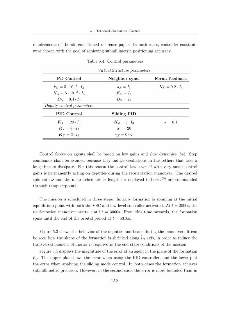
5 – Tethered Formation Control
requirements of the aforementioned reference paper. In both cases, controller constants
were chosen with the goal of achieving submillimetric positioning accuracy.
Table 5.4: Control parameters
Virtual Structure parameters
PD Control Neighbor sync. Form. feedback
kG = 5 · 10−3 · I3 kS = I3 KF = 0.2 · I3KG = 5 · 10−3 · I3 KS = I3
DG = 0.4 · I3 DS = I3
Deputy control parameters
PID Control Sliding PID
KP = 20 · I3 Kd = 3 · I3 κ = 0.1
KI = 53 · I3 αS = 20
KT = 3 · I3 γS = 0.02
Control forces on agents shall be based on low gains and slow dynamics [84]. Step
commands shall be avoided because they induce oscillations in the tethers that take a
long time to dissipate. For this reason the control law, even if with very small control
gains is permanently acting on deputies during the reorientation manouver. The desired
spin rate ν and the unstretched tether length for deployed tethers l(0) are commanded
through ramp setpoints.
The mission is scheduled in three steps. Initially formation is spinning at the initial
equilibrium point with both the VSC and low-level controller activated. At t = 2000s, the
reorientation manouver starts, until t = 3000s. From this time onwards, the formation
spins until the end of the orbital period at t = 5310s.
Figure 5.3 shows the behavior of the deputies and beads during the manouver. It can
be seen how the shape of the formation is shrinked along iR axis, in order to reduce the
transversal moment of inertia It required in the end state conditions of the mission.
Figure 5.4 displays the magnitude of the error of an agent in the plane of the formation
r1. The upper plot shows the error when using the PID controller, and the lower plot
the error when applying the sliding mode control. In both cases the formation achieves
submillimetric precision. However, in the second case, the error is more bounded than in
152
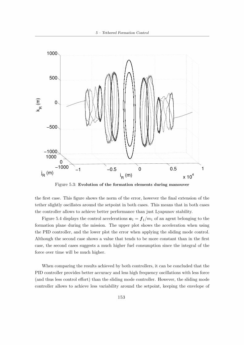
5 – Tethered Formation Control
−1 −0.5 0 0.5 1
x 104
−10000
1000−1000
−500
0
500
1000
iR
(m)jR
(m)
kR
(m
)
Figure 5.3: Evolution of the formation elements during manouver
the first case. This figure shows the norm of the error, however the final extension of the
tether slightly oscillates around the setpoint in both cases. This means that in both cases
the controller allows to achieve better performance than just Lyapunov stability.
Figure 5.4 displays the control accelerations a1 = f1/m1 of an agent belonging to the
formation plane during the mission. The upper plot shows the acceleration when using
the PID controller, and the lower plot the error when applying the sliding mode control.
Although the second case shows a value that tends to be more constant than in the first
case, the second cases suggests a much higher fuel consumption since the integral of the
force over time will be much higher.
When comparing the results achieved by both controllers, it can be concluded that the
PID controller provides better accuracy and less high frequency oscillations with less force
(and thus less control effort) than the sliding mode controller. However, the sliding mode
controller allows to achieve less variability around the setpoint, keeping the envelope of
153
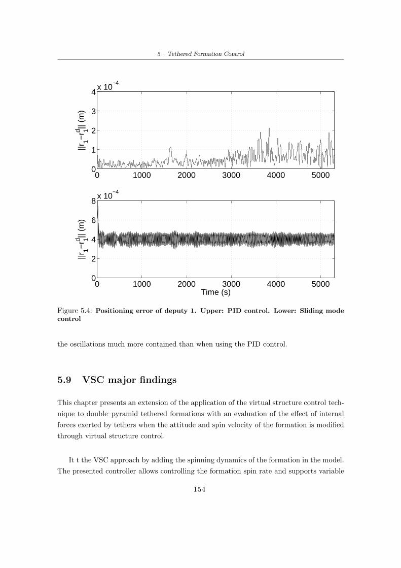
5 – Tethered Formation Control
0 1000 2000 3000 4000 50000
1
2
3
4x 10
−4||r
1−rd 1||
(m)
0 1000 2000 3000 4000 50000
2
4
6
8x 10
−4
||r1−
rd 1|| (m
)
Time (s)
Figure 5.4: Positioning error of deputy 1. Upper: PID control. Lower: Sliding modecontrol
the oscillations much more contained than when using the PID control.
5.9 VSC major findings
This chapter presents an extension of the application of the virtual structure control tech-
nique to double–pyramid tethered formations with an evaluation of the effect of internal
forces exerted by tethers when the attitude and spin velocity of the formation is modified
through virtual structure control.
It t the VSC approach by adding the spinning dynamics of the formation in the model.
The presented controller allows controlling the formation spin rate and supports variable
154

5 – Tethered Formation Control
0 1000 2000 3000 4000 50000
0.02
0.04
0.06
||a1||
(m/s
2 )
0 1000 2000 3000 4000 50000
0.02
0.04
0.06
||a1||
(m/s
2 )
Time (s)
Figure 5.5: Control acceleration of deputy 1. Upper: PID control. Lower: Slidingmode control
moment of inertia through a deployment/retrieval mechanism. Two alternatives are pre-
sented for accurate control of deputies in the presence of gravity gradient perturbation. An
scenario assesses the performance of the controller by showing successful submillimetric
positioning capability.
155

Chapter 6
Conclusions
The first part of this work introduces the topic, and shows the maturity of the state of the
art techniques for modeling the problem and the viability of the space tether applications,
including tethered cluster missions.
As part of the analysis of the effect of massive tethers in cluster dynamics, this work
shows that the effect of tether mass is almost negligible for open (HAS) formations, in
which case the massless model captures the dynamics of the cluster. It has a minimal
effect on the elongation and the angular separation of the tethers compared to the be-
havior of the massless model. Thus, a simplified model featuring purely elastic massless
tethers is sufficient for the purposes of preliminary mission analysis and possibly design
of formation control laws. Conversely, for closed formations, Closed-Hub-And-Spoke and
Double-Pyramid (CHAS and DP respectively), there are substantial differences in the be-
havior of the formation between the two models, which means that the simplified one may
miss relevant effects. The most noticeable effect is the monotonical bending of the external
tethers towards the exterior of the formation due mainly to the centriphugal force, and
in a lesser degree due to the effect of the gravitational force. This deformation of the
external tethers prevents the internal tethers from being fully extended, which is specially
noticeable in a DP cluster. The oscillation of internal tethers due to the to their inter-
mittent extension and loss of tension has a significant negative effect on the positioning
of the deputies, making closed formations with a parent body not suitable for accurate
agent positioning. Both in the CHAS and DP cases, the parent body drifts away from the
reference orbit due to the irregular motion of the agents.
As a novelty, the thesis proposes the use of circular shaped closed formations as an
156

6 – Conclusions
alternative to planar square shaped formations in order to eliminate the bouncing effect
on inner tethers, highlighted by the refined tethered formation model featuring massive
tethers. This type of formations provide improved rigidity that allows adjacent agents to
preserve their separation angle. At the same time, this configuration avoids the bouncing
problem and formation center of mass drift from the reference orbit.
One of the purposes of tethered formations is to establish a link between agents, such
that when the tethers remain taut, the formation replicates the behavior of an orbiting
spinning body exhibiting a natural equilibrium state. Three equilibrium conditions exist
for an spinning axisymmetrical rigid body. For practical reasons, this thesis is focused
on two scenarios: the Thomson equilibrium (for spinning formations lying in the orbital
plane), and the conical Likins-Pringle equilibrium (for formations facing the Earth). The
third possible equilibrium state, the hyperbolic Likins-Pringle, is not considered adequate
for most practical applications.
For tethered clusters with the spinning axis perpendicular to the orbital plane, the
Thomson equilibrium conditions define the constraints that ensure the equilibrium of the
formation. Furthermore, the HCW model used uncouples the planar of the the cross range
dynamics, therefore if the members of the formation lie in the orbital plane with null cross
track initial velocity, it can be guaranteed that the motion will be planar. This kind of sta-
bility is shown in all the planar formations lying in the orbital plane analyzed in this study.
For Earth-facing applications, the conical Likins-Pringle equilibrium is the most suit-
able state as it considers a spinning formation facing the Earth with a slight tilt angle with
respect of the local vertical. The elevation angle equilibrium condition depends essentially
on the moment of inertia of the formation and its spinning rate. For this purpose, and
due to its prolate axisymmetric characteristics, the DP formation is chosen as a suitable
candidate. An Earth-facing planar (oblate) formation does not maintain its axis pointing
to the Earth, as it tends to have the direction angular momentum pointing approximately
to an inertially fixed direction. This effect can be appreciated in all the Earth-facing pla-
nar formations analyzed in this study.
In order to evaluate the feasibility of tethered formations for missions in LEO, devi-
ations from the ideal cases of purely Keplerian motion in the neighborhood of a circular
reference orbit were analyzed, focusing on the effects of eccentricity of the reference orbit
and Earth’s oblateness. In particular, variation of orbital angular rate and distance from
157

6 – Conclusions
the Earth associated to an eccentric orbit cause a periodic variation of the gravity gradient
and inertial loads, whereas J2 effects represents the most relevant perturbation in LEO,
such that its effect needs to be accounted for even at a preliminary mission design stage.
For formations lying in the orbital plane, the spin rate of the formation with respect
to the orbital frame varies along the orbit, being higher at apogee (where orbit frame
angular speed is slower) and lower at perigee, due to the principle of conservation of an-
gular momentum. The effect of the gravitational gradient can also be observed in the
dynamics, being higher at perigee and lower at apogee. This affects the amplitude of the
elongation of tethers in open formations, and also in the oscillations of the bouncing of
external tethers in closed formations.
The J2 perturbation does not have a significant effect on the relative motion of the
deputies. However, in this study it can be clearly seen that it affects the trajectory of the
formation as a whole through a secular drift of the parent body. Due to tether tensions
on the initial instant of the simulation, the parent body is slightly shifted from the LVLH
origin, which leads subsequently to the parent body and the cluster drifting away in a
more noticeable way than in the unperturbed scenario case.
In order to address the control of tethered formations, a controller to stabilize an
Earth-facing double pyramid tethered cluster is proposed. The control strategy has a
double purpose: attitude control of the cluster and accurate position control of its agents.
For the purpose of attitude control, and taking advantage again of the similarities be-
tween a tethered cluster and a rigid body, the virtual structure approach is chosen as the
most suitable option. The formulation shown in this thesis augments the general virtual
structure equations valid for a static formation by adding the kinematics of a spinning
formation, since the original formulation is valid only to achieve a static final state. The
controller is designed to modify the spin rate and the moment of inertia of the formation
through a reeling mechanism, and therefore to be able to control the Likins-Pringle tilting
angle of the cluster.
For the derivation of the accurate positioning control law, the study initially discusses
different alternatives based on the state of the art of the robotics control literature. After
evaluating other alternatives, two control laws are chosen for this application: One based
on a PID controller and one based on the sliding mode control technique. For the sliding
mode based control, a proof of semi-global exponential stability is provided. Results of a
158

6 – Conclusions
representative simulation assess the viability of the control approach proposed leading to
a submillimetric positioning accuracy.
The work performed in this thesis could be extended by redesigning the fine position
control with the purpose of optimizing fuel consumption. The effect of electrodynamic
tethers is not within the scope of this work, although it could be studied in order to iden-
tify potential advantages related to the use of electrodynamic forces. An additional field
of investigation for future work on the subject stemming from the results presented in
this thesis is represented by the design of an active vibration control system that damps
oscillations originated by abrupt manouvers. The study of the potential effect of orbit de-
bris on a tethered structure and the possible reconfiguration options after a tether failure
could also complement the present study.
159

Nomenclature
Orbit Symbols
G = Gravitational constant
Me = Earth’s mass
Re = Radius of the Earth
µ = Earth’s standard gravitational parameter
TO = Orbital period
n = Orbital rate mean motion
a = Semimajor axis
i = Inclination
e = Eccentricity
Ea = Eccentric anomaly
θ = True anomaly
L = True longitude
M = Mean anomaly
λ = Mean longitude
Ω = Longitude of the ascending node
ωper = Argument of periapsis
tτ0 = Time when the satellite was at periapsis
R = Vector from center of the Earth to a given point
Rref = Vector from center of the Earth to a reference orbit.
ri = Position vector of a body i in the LVLH reference frame Rvi = Velocity vector of a body i in the LVLH reference frame R
160
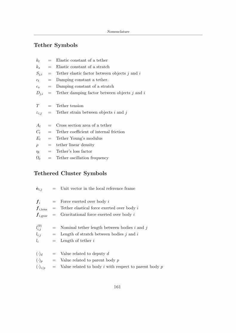
Nomenclature
Tether Symbols
kt = Elastic constant of a tether
ks = Elastic constant of a stratch
Sj,i = Tether elastic factor between objects j and i
ct = Damping constant a tether.
cs = Damping constant of a stratch
Dj,i = Tether damping factor between objects j and i
T = Tether tension
εi,j = Tether strain between objects i and j
At = Cross section area of a tether
Ct = Tether coefficient of internal friction
Et = Tether Young’s modulus
ρ = tether linear density
ηt = Tether’s loss factor
Ωt = Tether oscillation frequency
Tethered Cluster Symbols
ei,j = Unit vector in the local reference frame
f i = Force exerted over body i
f i,tens = Tether elastical force exerted over body i
f i,grav = Gravitational force exerted over body i
l(0)i,j = Nominal tether length between bodies i and j
li,j = Length of stratch between bodies j and i
li = Length of tether i
(·)d = Value related to deputy d
(·)p = Value related to parent body p
(·)i/p = Value related to body i with respect to parent body p
161

Nomenclature
mi = Mass of body i
mt = Mass of tether t
nb = Number beads on each tether
nd = Number of deputies in the formation
np = Number of parents in the formation
nt = Number of tethers in the formation
st = Number of stretches in tether t
qj = Generalized coordinate for object j
Qd = Raleigh function for damping force.
mi = Mass of object i
α = Pitch angle (in-plane angle for orbital motion)
β = Roll angle (out-of-plane angle for orbital motion)
α∗ = In-plane angle for normal plane motion
β∗ = Out-of-plane angle for normal plane motion
Dp = Distance of center of mass to parent body
rs = Factor of spin velocity
δj = In–plane angular orientation of deputy j with respect to axis i
γi,j = Angular separation between tether i and j
ω0 = Formation initial spin angular velocity
ωi/p = Local angular rotation velocity of object i with respect to parent body
ωi/p = Local angular rotation rate of object i with respect to parent body
h = Angular momentum vector
θ = Angular velocity of the LVLH reference frame
τ = Torque
kI = Inertia parameter
γ = Likins-Pringle tilting angle
Virtual Structure Control Symbols
Rd = Distance of parent body to center of the Earth
162

Nomenclature
qj = Generalized coordinate for object j
mi = Mass of object i
ri = Position error of body i
vi = Velocity error of body i
qi = Quaternion defining the orientation of body i
qi = Vector part of quaternion qi
qi = Scalar part of quaternion qi.
ωi = Spin velocity of agent i.
(·)di = Desired coordinate for agent i
(·)F = Coordinate related to Virtual Structure F
(·)Fi = Coordinate related to ith instance of Virtual Structure F .
(·)iF = Coordinate related to agent i relative to Virtual Structure F .
CRF = Direction cosine matrix between reference frame R and FCFS = Direction cosine matrix between reference frame F and Sα = Spin rate
φ = Axis of spin motion
λ = Formation expansion ratio.
λ = Formation expansion rate.
ν = Formation expansion straint.
kS , KS , DS = Agent synchronization constants.
kG, KG, ΓG = Proportional-Deriviative constants.
KF , DG = Formation feedback constants.
kα, kγ = Sliding mode control constants.
KP ,KI ,KD = Proportional, Integral and Derivative constant matrices.
S = Sliding surface.
Sr = Reference sliding surface.
Y rΘ = Regressor.
d(t) = External disturbance.
M = Inertia matrix
N = Coriolis/centrifugal terms matrix
P = Coupled elastic forces terms matrix
Q = Gravity gradient term matrix.
163
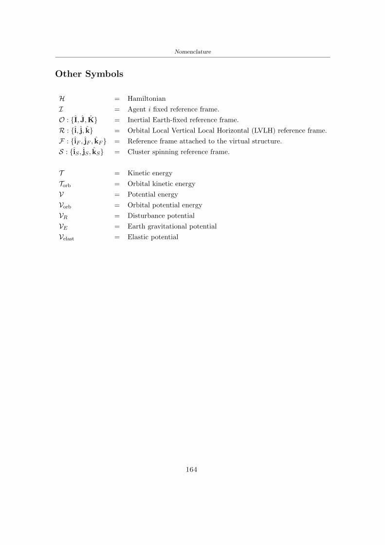
Nomenclature
Other Symbols
H = Hamiltonian
I = Agent i fixed reference frame.
O : I, J, K = Inertial Earth-fixed reference frame.
R : i, j, k = Orbital Local Vertical Local Horizontal (LVLH) reference frame.
F : iF , jF , kF = Reference frame attached to the virtual structure.
S : iS , jS , kS = Cluster spinning reference frame.
T = Kinetic energy
Torb = Orbital kinetic energy
V = Potential energy
Vorb = Orbital potential energy
VR = Disturbance potential
VE = Earth gravitational potential
Velast = Elastic potential
164
Acronyms
CHAS = Closed Hub-And-Spoke
DOF = Degree Of Freedom
DP = Double Pyramid
GAS = Global Asymptotic Stability
GPE = Gauss Planetary Equations
HAS = Hub-And-Spoke
HCW = Hill Clohessy Wiltshire
ISS = Input-to-State Stability
LEO = Low Earth Orbit
LVLH = Local Vertical Local Horizontal
PID = Proportional Integral Derivative
SEDS = Small Expendable Deployment System
SFF = Satellite Flight Formation
SPECS = Submillimeter Probe of the Evolution Cosmic Structure
TSS = Tethered Satellite System
VSC = Virtual Structure Control
165
Bibliography
[1] M.L. Cosmo, E.C. Lorenzini: Tethers in Space Handbook, Smithsonian
Astrophysical Observatory for NASA Marshall Space Flight Center, De-
cember 1997.
[2] E.M. Levin.: Dynamic Analysis of Space Tether Missions, Advances in
Astronautical Sciences, Volume 126, 2007.
[3] K.D. Kumar: Review of Dynamics and Control of Nonelectrodynamic
Tethered Satellite Systems, Journal of Spacecraft and Rockets, vol. 43,
no. 4, pp. 705720, Jul. 2006. http://dx.doi.org/10.2514/1.5479
[4] M.P. Cartmell, D.J. McKenzie: A review of space tether research,
Progress in Aerospace Sciences, vol. 44, no. 1, pp. 121, Jan. 2008.
http://dx.doi.org/10.1016/j.paerosci.2007.08.002
[5] H. Wen, D.P.Jin, H.Y. Hu: Advances in dynamics and control of tethered
satellite systems, Acta Mech Sin, vol. 24, no. 4, pp. 473473, Jul. 2008.
http://dx.doi.org/10.1007/s10409-008-0178-6
[6] Y. Chen, R. Huang, L. He, X. Ren, B. Zheng: A review of dy-
namical modelling and control for space tethers, Nonlinear Dyn, vol.
77, no. 4, pp. 10771099, Apr. 2014. http://dx.doi.org/10.1007/
s11071-014-1390-5
[7] E.C. Lorenzini, J.R. Sanmartin, Electrodynamic Tethers in Space, Sci-
entific American, vol. 291, no. 2, pp. 5057, Aug. 2004. http://dx.doi.
org/10.1038/scientificamerican0804-50
[8] K. Wormnes, R. Le Letty, L.Summerer, R. Schonenbor, O. Dubois-
Matra, E. Luraschi, A. Cropp, H. Krag and J. Delaval: ESA technologies
for space debris remediation. 6th European Conference on Space Debris,
Darmstadt, 2013.
[9] P. K. Aravind: The Physics of the Space Elevator, Am. J. Phys., vol.
75, no. 2, p. 125, 2007. http://dx.doi.org/10.1119/1.2404957
166

Bibliography
[10] M. Quadrelli: Modeling and Dynamics Analysis of Tethered Formations
for Space Interferometry, AAS/AIAA Spaceflight Mechanics Meeting,
Santa Barbara, CA, February 11-14, 2001.
[11] M. Quadrelli, F.Y. Hadaegh, E.C. Lorenzini, C. Bombardelli: Precision
Tethered Formations for LEO and Space Interferometry Applications,
16th International Symposium on Spaceflight Dynamics, Pasadena, CA,
December 3-7, 2001.
[12] R. Farley, D. Quinn: Tethered formation configurations: meeting the
scientific objectives of large aperture and interferometric science, AIAA
Space 2001 Conference and Exposition, Aug. 2001. http://dx.doi.
org/10.2514/6.2001-4770
[13] A. Pizarro-Chong, A. K. Misra: Dynamics of multi-tethered satellite for-
mations containing a parent body, Acta Astronautica, vol. 63, no. 1112,
pp. 11881202, Dec. 2008. http://dx.doi.org/10.1016/j.actaastro.
2008.06.021
[14] E. Kim, S.R. Vadali: Modeling Issues Related to Retrieval of Flexible
Tethered Satellite Systems, Journal of Guidance, Control, and Dynam-
ics, vol. 18, no. 5, pp. 11691176, Sep. 1995. http://dx.doi.org/10.
2514/3.21521
[15] P. Williams: Optimal control of a spinning double-pyramid Earth-
pointing tethered formation, Acta Astronautica, vol. 64, no. 1112,
pp. 11911223, Jun. 2009. http://dx.doi.org/10.1016/j.actaastro.
2009.01.014
[16] S.A. Schweighart, R.S. Sedwick: High-Fidelity Linearized J2 Model for
Satellite Formation Flight, Journal of Guidance, Control, and Dynam-
ics, vol. 25, no. 6, pp. 10731080, Nov. 2002. http://dx.doi.org/10.
2514/2.4986
[17] G. Inalhan, M. Tillerson, J.P. How: Relative Dynamics and Con-
trol of Spacecraft Formations in Eccentric Orbits, Journal of Guid-
ance, Control, and Dynamics, vol. 25, no. 1, pp. 4859, Jan. 2002.
http://dx.doi.org/10.2514/2.4874
[18] M. Sabatini, G.B. Palmerini: Linearized Formation-Flying Dynamics
in a Perturbed Orbital Environment, 2008 IEEE Aerospace Conference,
Mar. 2008. http://dx.doi.org/10.1109/aero.2008.4526271
[19] W. Ren, R. Beard: Decentralized Scheme for Spacecraft Formation Fly-
ing via the Virtual Structure Approach, Journal of Guidance, Control,
167

Bibliography
and Dynamics, vol. 27, no. 1, pp. 7382, Jan. 2004. http://dx.doi.org/
10.2514/1.9287
[20] R.W. Beard, J. Lawton, F.Y. Hadaegh: A Coordination Architecture for
Spacecraft Formation Control, IEEE Trans. Contr. Syst. Technol., vol.
9, no. 6, pp. 777790, 2001. http://dx.doi.org/10.1109/87.960341
[21] W. Ren, R. Beard: Virtual Structure Based Spacecraft Formation Con-
trol with Formation Feedback, AIAA Guidance, Navigation, and Control
Conference and Exhibit, Aug. 2002. http://dx.doi.org/10.2514/6.
2002-4963
[22] R. Beard, W. Ren: Formation feedback control for multiple spacecraft via
virtual structures, IEE Proceedings - Control Theory and Applications,
vol. 151, no. 3, pp. 357368, May 2004. http://dx.doi.org/10.1049/
ip-cta:20040484
[23] V. Parra-Vega, S. Arimoto, G. Hirzinger, P. Akella: Dynamic Slid-
ing PID Control for Tracking of Robot Manipulators: Theory and Ex-
periments, IEEE Transactions on Robotics and Automation, vol. 19,
no. 6, pp. 967976, Dec. 2003. http://dx.doi.org/10.1109/tra.2003.
819600
[24] Y. Choi, W.K. Chung, I.H. Suh: Performance and H-inf Optimality
of PID Trajectory Tracking Controller for Lagrangian Systems, IEEE
Transactions on Robotics and Automation, vol. 17, no. 6, pp. 857869,
2001. http://dx.doi.org/10.1109/70.976011
[25] Earth Observation Portal: https://directory.eoportal.org/web/
eoportal/satellite-missions/s/space-tethers
[26] Y. Chen, R. Huang, X. Ren, L. He, Y. He: History of the Tether Concept
and Tether Missions: A Review, ISRN Astronomy and Astrophysics,
vol. 2013, pp. 17, 2013. http://dx.doi.org/10.1155/2013/502973
[27] N. H. Stone, W. J. Raitt, K. H.Wright, Jr.: The TSS-1R Electrodynamic
Tether Experiment: Scientific and Technological Results. Advances in
Space Research, vol. 24, no. 8, pp. 10371045, Jan. 1999. http://dx.
doi.org/10.1016/s0273-1177(99)00551-7
[28] J.A. Carroll: SEDS Deployer Design and Flight Performance, Space
Programs and Technologies Conference and Exhibit, Sep. 1993. http:
//dx.doi.org/10.2514/6.1993-4764
[29] J. Glaese, R. Issa, and P. Lakshmanan: Comparison of SEDS-1 Pre-
Flight Simulations and Flight Data. Space Programs and Technologies
168

Bibliography
Conference and Exhibit, Sep. 1993. http://dx.doi.org/10.2514/6.
1993-4766
[30] M. Grassi, M.L. Cosmo: Attitude Dynamics of the Small Expendable-
Tether Deployment System. Acta Astronautica, vol. 36, no. 3,
pp. 141148, Aug. 1995. http://dx.doi.org/10.1016/0094-5765(95)
00093-f
[31] W. Barnds, S. Coffey, M. Davis, B. Kelm, W. Purdy: TiPS: Results of a
Tethered Satellite Experiment, Advances in the Astronautical Sciences,
AAS paper 97-600, 1997.
[32] K.T. Alfriend, W.J. Barnds, S.L. Coffey, L.M. Stuhrenberg: Attitude
and Orbit Determination of a Tethered Satellite System, Advances in
the Astronautical Sciences, AAS paper 95-351, 1995.
[33] http://www.thelivingmoon.com/41pegasus/02files/
Electrodynamic_01.html
[34] M. Kruijff, E. J. van der Heide: Qualification and in-flight demonstra-
tion of a European tether deployment system on YES2. Acta Astronau-
tica, vol. 64, no. 910, pp. 882905, May 2009. http://dx.doi.org/10.
1016/j.actaastro.2008.10.014
[35] D.A. Quinn, D.C. Folta: A Tethered Formation Flying Concept for the
SPECS Mission, 23rd Annual AAS Guidance and Control Conference,
February 2-6, 2000.
[36] C.D. Hall, M. Kim: Dynamics and Control of Rotating Tethered Satellite
Systems, Journal of Spacecraft and Rockets, vol. 44, no. 3, pp. 649659,
May 2007. http://dx.doi.org/10.2514/1.17065
[37] H. Goldstein, C. Poole, J. Safko, S.R. Addison, Classical Mechanics,
Addison Wesley, 2000. http://dx.doi.org/10.1119/1.1484149
[38] H. Schaub, J.L. Junkins: Analytical Mechanics of Space Systems, AIAA
Education Series, 2003. http://dx.doi.org/10.2514/4.861550.
[39] R. Battin: An Introduction to the Mathematics and Methods of Astro-
dynamics, AIAA Education Series, New York, 1987. http://dx.doi.
org/10.2514/4.861543.
[40] R.A. Broucke, P.J. Cefola: On The Equinoctial Orbit Elements, Celestial
Mechanics, vol. 5, no. 3, pp. 303310, May 1972. http://dx.doi.org/
10.1007/bf01228432
[41] M.J.H. Walker, B. Ireland, and J. Owens: A set of modified equinoctial
orbit elements, Celestial Mechanics, vol. 36, no. 4, pp. 409419, Aug.
169

Bibliography
1985. http://dx.doi.org/10.1007/bf01227493
[42] O. Stone: On the solution of Delaunay’s canonical system of equations,
The Astronomical Journal, vol. 20, no.2, 1899. http://dx.doi.org/
10.1086/103072
[43] F.T. Geyling, H.R. Westerman: Introduction to Orbital Mechanics,
Addison-Wesley Aerospace Series, 1971.
[44] W.H. Clohessy, R.S. Wiltshire: Terminal guidance system for satellite
rendezvous, Journal of the Aerospace Sciences, vol. 27, no. 9, pp. 653658,
Sep. 1960. http://dx.doi.org/10.2514/8.8704
[45] S.S. Vaddi, S.R. Vadali, K. T. Alfriend: Formation Flying: Accommo-
dating Nonlinearity and Eccentricity Perturbations, Journal of Guid-
ance, Control, and Dynamics, vol. 26, no. 2, pp. 214223, Mar. 2003.
http://dx.doi.org/10.2514/2.5054
[46] D.F. Lawden: Optimal Trajectories for Space Navigation, Butterworths,
London, pp. 79–86, 1963. http://dx.doi.org/10.2307/3611765
[47] J.F. Tschauner, P.R. Hempel: Rendezvous zu einemin elliptischer Bahn
umlaufenden Ziel, Astronautica Acta, Vol. 11, No. 2, pp. 104109, 1965.
[48] T.E. Carter: New Form for the Optimal Rendezvous Equations near a
Keplerian Orbit, Journal of Guidance, Control, and Dynamics, vol. 13,
no. 1, pp. 183186, Jan. 1990. http://dx.doi.org/10.2514/3.20533
[49] T.E. Carter, M. Humi: Fuel-Optimal Rendezvous near a Point in Gen-
eral Keplerian Orbit. Journal of Guidance, Control, and Dynamics,
vol. 10, no. 6, pp. 567573, Nov. 1987. http://dx.doi.org/10.2514/
3.20257
[50] Y. Ren, J. J. Masdemont, M. Marcote, and G. Gomez: Computation
of analytical solutions of the relative motion about a Keplerian elliptic
orbit, Acta Astronautica, vol. 81, no. 1, pp. 186199, Dec. 2012. http:
//dx.doi.org/10.1016/j.actaastro.2012.07.026
[51] H. Schaub: Incorporating Secular Drifts into the Orbit Element Dif-
ference Description of Relative Orbits, 13th AAS/AIAA Space Flight
Mechanics Meeting, February 9-13, 2003.
[52] H. Schaub, S. R. Vadali, J. L. Junkins, and K. T. Alfriend: Spacecraft
formation flying control using mean orbital elements, Journal of the
Astronautical Sciences, vol. 48, No. 1, pp. 69-87, Jan-March, 2000.
[53] H. Schaub and T. Alfriend: J2 invariant relative orbits for spacecraft for-
mations, Flight Mechanics Symposium, (NASA Goddard Space Flight
170

Bibliography
Center, Greenbelt, MD), pp. 125-139, 1999.
[54] H. Yan, K.T. Alfriend, S.R. Vadali, P. Sengupta: Optimal Design of
Satellite Formation Relative Motion Orbits Using Least-Squares Meth-
ods, Journal of Guidance, Control, and Dynamics, vol. 32, no. 2, pp.
599604, Mar. 2009. http://dx.doi.org/10.2514/1.35044
[55] R.R. Bate, D.D. Mueller, J.E. White: Fundamentals of Astrodynamics,
Dover, New York, 1971.
[56] S.R.Vadali, K.T.Alfriend, S.Vaddi: Hill’s equation, Mean Orbital Ele-
ments, and Formation Flying of Satellites, Advances in the Astronauti-
cal Sciences, AAS 00–258, 2000.
[57] H. Schaub: Relative Orbit Geometry Through Classical Orbit Element
Differences, Journal of Guidance, Control, and Dynamics, vol. 27, no.
5, pp. 839848, Sep. 2004. http://dx.doi.org/10.2514/1.12595
[58] H. Schaub and K. T. Alfriend: Hybrid Cartesian and Orbit Element
Feedback Law for Formation Flying Spacecraft, Journal of Guidance,
Control, and Dynamics, vol. 25, no. 2, pp. 387393, Mar. 2002.
[59] M. Capderou: Satellites: orbits and missions, Volume 1, Springer, 2005.
[60] V.A. Chobotov: Orbital Mechanics, AIAA Education Series, 2002.
http://dx.doi.org/10.2514/4.862250
[61] K.T. Alfriend, H. Schaub: Dynamics and Control of Spacecraft For-
mations: Challenges and Some Solutions, Journal of the Astronautical
Sciences, vo.l 48, no. 2, pp. 249-267, April-September 2000.
[62] K. Yamada, T. Shima, S. Yoshikawa: Effect of the J2 Perturbation on
Relative Spacecraft Position in Near-Circular Orbits, Journal of Guid-
ance, Control, and Dynamics, vol. 33, no. 2, pp. 584590, Mar. 2010.
http://dx.doi.org/10.2514/1.47436
[63] D.W. Gim, K.T. Alfriend: State Transition Matrix of Relative Motion
for the Perturbed Noncircular Reference Orbit, Journal of Guidance,
Control, and Dynamics, vol. 26, no. 6, pp. 956971, Nov. 2003. http:
//dx.doi.org/10.2514/2.6924
[64] K.T. Alfriend, H. Yan: Evaluation and Comparison of Relative Motion
Theories, Journal of Guidance, Control, and Dynamics, vol. 28, no. 2,
pp. 254261, Mar. 2005. http://dx.doi.org/10.2514/1.6691
[65] J.A. Roberts, P.C.E. Roberts: The Development of High Fidelity Lin-
earized Models for Satellite Formation Flying Control, Advances in the
Astronautical Sciences, Vol. 119, Part 1, pp. 913–934, 2004.
171
Bibliography
[66] M. Sabu Sebastian, K.C. Unnikrishnan, S. Narayanan: Viscoelastic
properties of Kevlar®-29 fabric tape strength member, Mechanics of Ma-
terials, vol. 40, no. 11, pp. 949960, Nov. 2008. http://dx.doi.org/10.
1016/j.mechmat.2008.05.002
[67] Hughes, P.C.: Spacecraft Attitude Dynamics, Dover Publications, 2004.
[68] G. Genta: Vibration Dynamics and Control, Springer, 2009, DOI:
10.1007/978-0-387-79580-5.
[69] V.V. Beletsky, E.M. Levin: Dynamics of space tether systems, Advances
in Astronautical Sciences, Volume 83, 1993.
[70] K.K. Mankala, S.K. Agrawal: Dynamic Modeling and Simulation of
Satellite Tethered Systems, Journal of Vibration and Acoustics, vol. 127,
no. 2, p. 144, 2005. http://dx.doi.org/10.1115/1.1891811
[71] M. Krupa, W. Poth, M. Schagerl, A. Steindl, W. Steiner, H. Troger, G.
Wiedermann: Modelling, Dynamics and Control of Tethered Satellite
Systems, Nonlinear Dyn, vol. 43, no. 12, pp. 7396, Jan. 2006. http:
//dx.doi.org/10.1007/s11071-006-0752-z
[72] M. Krupa, M. Schagerl, A. Steindl, P. Szmolyan, H.Troger: Relative
equilibria of tethered satellite systems and their stability for very stiff
tethers, Dynamical Systems, vol. 16, no. 3, pp. 253278, Sep. 2001. http:
//dx.doi.org/10.1080/14689360117072
[73] Y. Yan, A.K. Misra, N. Oshiro, T. Yamamoto: Modeling of the Dy-
namics of N-Body Tethered Satellite Systems, Asia-Pacific Vibration
Conference, Kyongju, Korea, November 9-13, 1997.
[74] F. Dignath, W. Schiehlen: Control of the Vibrations of a Tethered
Satellite System, Journal of Applied Mathematics and Mechanics,
vol. 64, no. 5, pp. 715722, Jan. 2000. http://dx.doi.org/10.1016/
s0021-8928(00)00100-3
[75] S.G. Tragesser: Formation Flying with Tethered Spacecraft. Astro-
dynamics Specialist Conference, Aug. 2000. http://dx.doi.org/10.
2514/6.2000-4133
[76] S.G. Tragesser, A. Tuncay: Orbital Design of Earth-Oriented Tethered
Satellite Formations. AIAA/AAS Astrodynamics Specialist Conference
and Exhibit, Aug. 2002. http://dx.doi.org/10.2514/6.2002-4641
[77] A.P. French: Vibrations and Waves, The MIT Introductory Physics
Series. The Massachusetts Institute of Technology, 1966.
172

Bibliography
[78] J. Pelaez: On the Dynamics of the Deployment of a Tether from an Or-
biter - I. Basic Equations, Acta Astronautica, vol. 36, no. 2, pp. 113122,
Jul. 1995. http://dx.doi.org/10.1016/0094-5765(95)00045-2
[79] J. Pelaez: On the Dynamics of the Deployment of a Tether from an
Orbiter - II. Exponential Deployment, Acta Astronautica, vol. 36, no. 6,
pp. 313335, Sep. 1995. http://dx.doi.org/10.1016/0094-5765(95)
00117-4
[80] N.N. Smirnov, Yu.A. Demyanov, A.V. Zvyaguin, A.A. Malashin, A.A.
Luzhin: Dynamical simulation of tether in orbit deployment, Acta As-
tronautica, vol. 67, no. 34, pp. 324332, Aug. 2010. http://dx.doi.org/
10.1016/j.actaastro.2010.02.020
[81] A. Steindl, H. Troger: Optimal Control of Deployment of a Tethered
Subsatellite, Nonlinear Dynamics 31: 257274, 2003.
[82] A. Steindl, W. Steiner, H. Troger: Optimal Control of Retrieval of a
Tethered Subsatellite, IUTAM Symposium on Chaotic Dynamics and
Control of Systems and Processes in Mechanics, pp. 441450, 2005. http:
//dx.doi.org/10.1007/1-4020-3268-4_41
[83] A.E. Bryson, Y.-C. Ho: Applied Optimal Control: Optimization Esti-
mation and Control, Taylor & Francis, 1988.
[84] K. Nakaya, M. Iai, K. Omagari, H. Yabe, S. Matunaga: Formation De-
ployment Control for Spinning Tethered Formation Flying -Simulations
and Ground Experiments-, AIAA Guidance, Navigation, and Control
Conference and Exhibit, Aug. 2004. http://dx.doi.org/10.2514/6.
2004-4896
[85] B.S. Yu, D.P. Jin: Deployment and retrieval of tethered satellite sys-
tem under J2 perturbation and heating effect, Acta Astronautica, vol.
67, no. 78, pp. 845853, Oct. 2010. http://dx.doi.org/10.1016/j.
actaastro.2010.05.013
[86] J.L. Tang, G.X. Ren, W.D. Zhu, H. Ren: Dynamics of variable-length
tethers with application to tethered satellite deployment, Communica-
tions in Nonlinear Science and Numerical Simulation, vol. 16, no.
8, pp. 34113424, Aug. 2011. http://dx.doi.org/10.1016/j.cnsns.
2010.11.026
[87] P. M. Bainum, V. K. Kumar: Optimal Control of the Shuttle–Tethered–
Subsatellite System, Acta Astronautica, vol. 7, no. 12, pp. 13331348,
Dec. 1980. http://dx.doi.org/10.1016/0094-5765(80)90010-7
173

Bibliography
[88] A.K. Misra: Dynamics and control of tethered satellite systems, Acta
Astronautica, vol. 63, no. 1112, pp. 11691177, Dec. 2008. http://dx.
doi.org/10.1016/j.actaastro.2008.06.020
[89] A. Pizarro-Chong, A. K. Misra: Dynamics of a Multi-Tethered Satel-
lite Formation, AIAA/AAS Astrodynamics Specialist Conference and
Exhibit, Aug. 2004. http://dx.doi.org/10.2514/6.2004-5308
[90] P. Williams: Dynamics and Control of Spinning Tethers for Rendezvous
in Elliptic Orbits, Journal of Vibration and Control, vol. 12, no. 7, pp.
737771, Jul. 2006. http://dx.doi.org/10.1177/1077546306065710
[91] P. Williams: Libration Control of Tethered Satellites in Elliptical Orbits,
Journal of Spacecraft and Rockets, vol. 43, no. 2, pp. 476479, Mar. 2006.
http://dx.doi.org/10.2514/1.17499
[92] H.A. Fujii, W. Ichiki: Nonlinear Dynamics of the Tethered Subsatellite
System in the Station Keeping Phase, Journal of Guidance, Control,
and Dynamics, vol. 20, no. 2, pp. 403406, Mar. 1997. http://dx.doi.
org/10.2514/2.4057
[93] V. A. Zlatoustov, A. P. Markeev: Stability of Planar Oscillations of a
Satellite in an Elliptical Orbit, Celestial Mechanics, vol. 7, no. 1, pp.
3145, Jan. 1973. http://dx.doi.org/10.1007/bf01243507
[94] A. Celletti, V. Sidorenko: Some properties of the dumbbell satellite at-
titude dynamics, Celest Mech Dyn Astr, vol. 101, no. 12, pp. 105126,
Mar. 2008. http://dx.doi.org/10.1007/s10569-008-9122-0
[95] H.A. Fujii, W. Ichiki, S. Suda, T.R. Watanabe: Chaos Analysis on Li-
brational Control of Gravity-Gradient Satellite in Elliptic Orbit, Journal
of Guidance, Control, and Dynamics, vol. 23, no. 1, pp. 145146, Jan.
2000. http://dx.doi.org/10.2514/2.4500
[96] A. Burov, I. Kosenko: Dumb–Bell of Variable Length in an Elliptic
Orbit: Relative Equilibria, Periodicity, and Chaos. Proceedings, 4th
Chaotic Modelling and Simulation International Conference, 31 May
- 3 June, 2011.
[97] A. Burov, I. Kosenko: On planar oscillations of a body with a vari-
able mass distribution in an elliptic orbit. Proceedings of the Insti-
tution of Mechanical Engineers, Part C: Journal of Mechanical En-
gineering Science, vol. 225, no. 10, pp. 22882295, Sep. 2011. http:
//dx.doi.org/10.1177/0954406211404327
[98] D.P. Jin and H. Y. Hu: Optimal Control of a Tethered Subsatellite of
174
Bibliography
Three Degrees of Freedom, Nonlinear Dyn, vol. 46, no. 12, pp. 161178,
Aug. 2006. http://dx.doi.org/10.1007/s11071-006-9021-4
[99] J.R. Sanmartin, E.C. Lorenzini, M. Martinez-Sanchez, A Re-
view of Electrodynamic Tethers for Space Applications, 44th
AIAA/ASME/SAE/ASEE Joint Propulsion Conference; Exhibit, Jul.
2008. http://dx.doi.org/10.2514/6.2008-4595
[100] J.R. Sanmartin, E.C. Lorenzini, M. Martinez-Sanchez: Electrodynamic
Tether Applications and Constraints, Journal of Spacecraft and Rockets,
vol. 47, no. 3, pp. 442456, May 2010. http://dx.doi.org/10.2514/1.
45352
[101] M. Sanjurjo-Rivo and J. Pela’ez: Energy Analysis of Bare Electrody-
namic Tethers, Journal of Propulsion and Power, vol. 27, no. 1, pp.
246256, Jan. 2011. http://dx.doi.org/10.2514/1.48168
[102] V.A. Chobotov and D.L. Mains: Tether Satellite System Collision
Study, Acta Astronautica, vol. 44, no. 712, pp. 543551, Apr. 1999.
http://dx.doi.org/10.1016/s0094-5765(99)00098-3
[103] I. Kim, H. Hirayama, T. Hanada: Practical guidelines for electro-
dynamic tethers to survive from orbital debris impacts, Advances in
Space Research, vol. 45, no. 10, pp. 12921300, May 2010. http://dx.
doi.org/10.1016/j.asr.2010.01.012
[104] G.L. Gittins, G.G. Swinerd, H.G. Lewis, D.N. Williams: A study of
debris impact collision probabilities to space tethers, Advances in Space
Research, vol. 34, no. 5, pp. 10801084, Jan. 2004. http://dx.doi.org/
10.1016/j.asr.2003.01.013
[105] J. Pearson, E. Levin, J. Oldson, H. Wykes: Lunar space elevators for
cislunar space development, NASA Research Subaward No.: 07605-
003-034, 2005. http://www.niac.usra.edu/files/studies/final_
report/1032Pearson.pdf
[106] DuPont™ Advanced Fiber Systems: Kevlar® aramid fiber technical
guide, www.dupont.com
[107] M.M. Wallace, C. W. Bert: Experimental determination of dynamic
Young’s modulus and damping of an aramid-fabric/polyester composite
material, Proc. Okla. Acad. Sci. 59:98-101, 1979.
[108] K.D. Godard, A. Kumar, B. Tan: Nonlinear optimal control of tethered
satellite systems using tether offset in the presence of tether failure,
Acta Astronautica, vol. 66, no. 910, pp. 14341448, May 2010. http:
175

Bibliography
//dx.doi.org/10.1016/j.actaastro.2009.10.037
[109] S.-J. Chung, J.-J. Slotine, D. W. Miller: Nonlinear Model Reduction and
Decentralized Control of Tethered Formation Flight, Journal of Guid-
ance, Control, and Dynamics, vol. 30, no. 2, pp. 390400, Mar. 2007.
http://dx.doi.org/10.2514/1.21492
[110] J.A. Carroll, J.C. Olson: Tethers for Small Satellite Applications,
AIAA/USU Small Satellite Conference in Logan, Utah, 1995.
[111] R. Orban: Advances in space tether materials, 3rd Tethers in Space/
Toward Flight International Conference, May 1989.
[112] D.D. Tomlin, G.C. Faile, K.B. Hayashida, C.L. Frost, C.Y. Wagner,
M.L. Mitchell, J.A. Vaughn, and M.J. Galuska: Space Tethers: Design
Criteria, NASA Technical Memorandum 108537, 1997.
[113] A.B. DeCou: Tether Static Shape for Rotating Multimass, Multitether,
Spacecraft for ’Triangle’ Michelson Interferometer, Journal of Guidance,
Control and Dynamics, vol. 2, no. 2, pp. 273-275, March 1989. http:
//dx.doi.org/10.2514/3.20401
[114] A. Amour, A.K. Misra, V.J. Modi: Equilibrium Configurations and
Their Stability in Three-Dimensional Motion of Three-Body Tethered
Systems, International Astronautical Federation, IAF-01-A.4.07, 2001.
[115] D.A. Quinn, R.E. Farley: Tethered Formation Configurations: Meeting
the Scientific Objectives of Large Aperture and Interferometric Science,
AIAA Space 2001 Conference and Exposition, Aug. 2001. http://dx.
doi.org/10.2514/6.2001-4770
[116] T. Williams, K. Moore: Dynamics of Tethered Satellite Formations,
AAS 02-198, AAS/AIAA Spaceflight Mechanics Meeting, Jan. 2002.
[117] M. Sabatini, G.B. Palmerini, Dynamics of a 3D Rotating Tethered For-
mation Flying Facing the Earth, IEEE Aerospace Conference, 2007.
http://dx.doi.org/10.1109/aero.2007.352671
[118] D. McKenzie, M. Cartmell, G. Radice, and M. Vasile. Space webs
final report 05-4109a. Ariadna study 05-4109a, University of Glas-
gow and ESA, 2006. URL http://www.esa.int/gsp/ACT/doc/ARI/
ARIStudyReport/ACT-RPT-MAD-ARI-05-4109b-SpaceWebs-Glasgow.
[119] A.D. Guerman, G. Smirnov, P. Paglione, A. M. Vale Seabra: Stationary
Configurations of a Tetrahedral Tethered Satellite Formation, Journal of
Guidance, Control, and Dynamics, vol. 31, no. 2, pp. 424428, Mar. 2008.
176

Bibliography
http://dx.doi.org/10.2514/1.31979
[120] S.M. Yoo, S.Y. Park: Determination of Initial Conditions for Tetrahe-
dral Satellite Formation, Journal of Astronomy and Space Sciences, vol.
28, no. 4, pp. 285290, Dec. 2011. http://dx.doi.org/10.5140/jass.
2011.28.4.285
[121] G. Avanzini, M. Fedi: Refined dynamical analysis of multi-tethered
satellite formations, Acta Astronautica, vol. 84, pp. 3648, Mar. 2013.
http://dx.doi.org/10.1016/j.actaastro.2012.10.031
[122] V.V. Beletskii, V.V.: Motion of an Artificial Satellite About its Center
of Mass, Israel Program for Scientific Translations, NASA-TT-F-429,
TT-67-51366, 1966.
[123] M. Fedi, G. Avanzini, Virtual Structure Formation Control for Tethered
Satellite Formations, 7th International Workshop on Satellite Constel-
lations and Formation Flying, 2013
[124] P. Erichsen: Performance Evaluation of Spacecraft Propulsion Systems
in Relation to Mission Impulse Requirements, Second European Space-
craft Propulsion Conference, Proceedings of the conference, 27-29 May
1997 in Noordwijk, The Netherlands. ESA SP-398.
[125] R. H. Frisbee: Advanced Space Propulsion for the 21st Century, Journal
of Propulsion and Power, vol. 19, no. 6, pp. 11291154, Nov. 2003.
[126] Chobotov, V.A.: Spacecraft Attitude Dynamics and Control, Krieger
Publishing Company, 1991.
[127] J. Gonzalez del Amo: European Space Agency Activities in Electric
Propulsion, The 33st International Electric Propulsion Conference, The
George Washington University, USA, 2013.
[128] T. Rupp, S. D’Amico, O. Montenbruck, E. Gill: Autonomous Forma-
tion Flying at DLR’s German Space Operations Center (GSOC), 58th
International Astronautical Congress, 2007-09-24 - 2007-09-28, Hyder-
abad.
[129] A. Garcia-Rodriguez, et al: GNSS in Space, Part 2: Formation Flying
Radio Frequency Techniques and Technology, Inside GNSS Jan./Feb.
2009, http://www.insidegnss.com/node/1123
[130] J.R. Wertz: Spacecraft Attitude Determination and Control, Kluwer
Academic Publishers, 1990.
[131] M. J. Sidi: Spacecraft Dynamics and Control. A Practical Engineering
Approach, Cambridge University Press, 1997.
177

Bibliography
[132] Scott R. Starin: Attitude Determination and Control Systems, NASA
report. http://ntrs.nasa.gov/archive/nasa/casi.ntrs.nasa.gov/
20110007876.pdf
[133] A. Pizarro-Chong: Dynamics of multi-tethered satellite formations,
VDM, 2008.
[134] K.A. Vogel: Dynamics and Control of Tethered Satellite Formations for
the Purpose of Space-Based Remote Sensing, Ph.D. Thesis, Air Force
Institute of Technology, AFIT/DS/ENY/06-04, 2006.
[135] G. Avanzini, M. Fedi: Effects of eccentricity of the reference orbit on
Multi-Tethered Satellite Formations, Acta Astronautica, vol. 94, no.
1, pp. 338350, Jan. 2014. http://dx.doi.org/10.1016/j.actaastro.
2013.03.019
[136] G. Avanzini, M. Fedi: Effects of J2 perturbations on multi-tethered
satellite formations. AAS 11-631, AAS/AIAA Astrodynamics Specialist
Conference, 2011.
[137] K.T. Alfriend, S.R. Vadali, P. Gurfil, J. P. How, L. S. Breger: Spacecraft
Formation Flying. Dynamics, control and navigation, Elsevier 2010.
[138] D.P. Scharf, F.Y. Hadaegh, S.R. Ploen: A Survey of Spacecraft Forma-
tion Flying Guidance and Control (Part I): Guidance, Proceedings of
the 2003 American Control Conference, 2003. http://dx.doi.org/10.
1109/acc.2003.1239845
[139] D.P. Scharf, F.Y. Hadaegh, S.R. Ploen: A Survey of Spacecraft Forma-
tion Flying Guidance and Control (Part II): Control, Proceedings of the
American Control Conference, 2004.
[140] R. Bevilacqua, M. Romano, F. Curti: Decoupled-natural-dynamics
Model for the Relative Motion of two Spacecraft without and with J2
Perturbation, Nonlinear Dynamics and Systems Theory, 10 (1) 1120,
2010.
[141] H. Liang, J. Wang, Z. Sun Robust decentralized coordinated attitude
control of spacecraft formation, Acta Astronautica, vol. 69, no. 56, pp.
280288, Sep. 2011. http://dx.doi.org/10.1016/j.actaastro.2011.
03.018
[142] R. Pongvthithum, S.M. Veres, S.B. Gabriel, E. Rogers: Universal adap-
tive control of satellite formation flying, International Journal of Con-
trol, vol. 78, no. 1, pp. 4552, Jan. 2005. http://dx.doi.org/10.1080/
00207170412331330887
178
Bibliography
[143] R. Kristiansen, P. J. Nicklasson: Spacecraft formation flying: A review
and new results on state feedback control, Acta Astronautica, vol. 65,
no. 1112, pp. 15371552, Dec. 2009. http://dx.doi.org/10.1016/j.
actaastro.2009.04.014
[144] Y. Xu, N. Fitz-Coy, Rick Lind, A. Tatsch: µ Control for Satellites
Formation Flying, J. Aerosp. Eng., vol. 20, no. 1, pp. 1021, Jan. 2007.
http://dx.doi.org/10.1061/(asce)0893-1321(2007)20:1(10)
[145] J.T. Wen, K. Kreutz-Delgado: The Attitude Control Problem, IEEE
Trans. Automat. Contr., vol. 36, no. 10, pp. 11481162, 1991. http:
//dx.doi.org/10.1109/9.90228
[146] Wie, B.: Space Vehicle Dynamics and Control, American Institute of
Aeronautics and Astronautics, Inc., Reston, VA, 1998.
[147] G. Avanzini, G. de Matteis, V. Tarantini: Control of an Orbiting For-
mation of Satellites Using the Virtual Structure Approach, AAS 05-276,
AAS/AIAA Astrodynamics Specialists Conference, August 7-11, 2005.
[148] Y. Kim, C. Ahn: Point Targeting of Multisatellites via a Virtual Struc-
ture Formation Flight Scheme, Journal of Guidance, Control, and Dy-
namics, vol. 32, no. 4, pp. 13301344, Jul. 2009. http://dx.doi.org/
10.2514/1.39537
[149] S.-J. Chung, D. W. Miller: Propellant-Free Control of Tethered For-
mation Flight, Part 1: Linear Control and Experimentation, Journal of
Guidance, Control, and Dynamics, vol. 31, no. 3, pp. 571584, May 2008.
http://dx.doi.org/10.2514/1.32188
[150] S.-J. Chung, J.-J. Slotine, D. W. Miller: Propellant-Free Control of
Tethered Formation Flight, Part 2: Nonlinear Underactuated Con-
trol, Journal of Guidance, Control, and Dynamics, vol. 31, no. 5, pp.
14371446, Sep. 2008. http://dx.doi.org/10.2514/1.32189
[151] S.-J. Chung, J.-J. Slotine, D. W. Miller: New Control Strategies for
Underactuated Tethered Formation Flight Spacecraft, AIAA Guidance,
Navigation and Control Conference and Exhibit, Aug. 2007. http://
dx.doi.org/10.2514/6.2007-6858
[152] K. Nakaya, S. Matunaga: On Attitude Maneuver of Spinning Tethered
Formation Flying Based on Virtual Structure Method, AIAA Guidance,
Navigation, and Control Conference and Exhibit, Aug. 2005. http://
dx.doi.org/10.2514/6.2005-6088
179

Bibliography
[153] Z. Qu, J. Dorsey: Robust Tracking Control of Robots by a Linear Feed-
back Law, IEEE Trans. Automat. Contr., vol. 36, no. 9, pp. 10811084,
1991. http://dx.doi.org/10.1109/9.83543
[154] Siciliano, B., Khatib, O., Springer Handbook of Robotics, Springer, 2008.
[155] D.S. Bernstein, S.P. Bhat: Lyapunov Stability, Semistability, and
Asymptotic Stability of Matrix Second-Order Systems, Proceedings of
1994 American Control Conference - ACC 94, 1994. http://dx.doi.
org/10.1109/acc.1994.752501
[156] J.-J. Slotine, W. Li: Applied Nonlinear Control, Englewood Cliffs, NJ:
Prentice-Hall, 1991.
[157] Haddad, W.M., Chellaboina, V.: Nonlinear Dynamical Systems and
Control. A Lyapunov-Based Approach, Princeton University Press,
2008.
[158] J.J. Slotine, W. Li: On the Adaptive Control of Robot Manipulators,
The International Journal of Robotics Research, vol. 6, no. 3, pp. 4959,
Sep. 1987. http://dx.doi.org/10.1177/027836498700600303
[159] P. Tomei: Adaptive PD controller for robot manipulators, IEEE Trans-
actions on Robotics and Automation, vol. 7, no. 4, pp. 565570, 1991.
http://dx.doi.org/10.1109/70.86088
[160] R. Kelly: PD control with desired gravity compensation of robot ma-
nipulators: A review, The International Journal of Robotics Research,
vol. 16, no. 5, pp. 660672, Oct. 1997. http://dx.doi.org/10.1177/
027836499701600505
[161] A. Loria, E. Lefeber, H. Nijmeijer: Global Asymptotic Stability of Robot
Manipulators with Linear PID and PI2D Control, SACTA, pp. 138-149,
2000.
[162] J.A. Ramirez, I. Cervantes, R. Kelly: PID regulation of robot ma-
nipulators: Stability and Performance, Systems and Control Letters,
vol. 41, no. 2, pp. 7383, Oct. 2000. http://dx.doi.org/10.1016/
s0167-6911(00)00038-4
[163] J.T. Wen, S. Murphy: PID control for robot manipulators, CIRSSE
Document 54, Rensselaer Polytechnic Institute, May 1990.
[164] Y. Choi, W.K. Chung: PID Trajectory Tracking Control for Mechani-
cal Systems, Lecture Notes in Control and Information Sciences, 2004.
http://dx.doi.org/10.1007/b10906
[165] H.A. Fujii, T. Watanabe, P. M. Trivailo: Wave-absorbing control of
180

Bibliography
transverse vibration of Tether Systems, The Journal of the Astronautical
Sciences, Vol. 51, No. 3, pp. 249-259, July-September 2003.
[166] P. Williams: Optimal Deployment and Offset Control for a Spinning
Flexible Tethered Formation, AIAA Guidance, Navigation, and Control
Conference and Exhibit, Aug. 2006. http://dx.doi.org/10.2514/6.
2006-6041
[167] S.J. Chung and D.W. Miller: Nonlinear Control and Synchronization
of Multiple Lagrangian Systems with Application to Tethered Formation
Flight Spacecraft, Ph.D. Thesis, Massachusetts Institute of Technology,
2007.
[168] A.B. DeCou: Attitude and Tether Vibration Control in Spinning Teth-
ered Triangles for Orbiting Interferometry, The Journal of the Astro-
nautical Sciences, Vol. 41, No. 3, July-September 1993, pp. 373-398.
181