Dynamics and variability of the coupled

atmosphere–ocean system

Johan Nilsson

Department of Meteorology

Bert Bolin Centre for Climate Research

Stockholm University, Sweden

1

What is coupled dynamics/variability?

One definition: the dynamics under (partly) fixed surface fluxes; i.e.a change of the fluid state does not change the fluxes.

An ocean model with fixed surface fluxes of momentum, heat andfreshwater give some flavor of uncoupled ”ocean dynamics”. How-ever, these fluxes implicitly assumes the presence of an atmosphere.

Venus and Mars (or a model with zero surface heat flux) are proto-types for uncoupled ”atmospheric dynamics”.

Is a hypothetical liquid ocean beneath Mars’ feeble atmosphere aprototype for uncoupled dynamics? What would the energy-transportpartitioning be on this planet?

2

Outline: Part 1

1. Radiation balance and energy transport; re-iterate the arguments

of one (1978).

2. The time-mean partitioning of the energy transport between the

atmosphere and the ocean; simulations and conceptual models.

3. Hurricanes and other speculative ideas.

4. Time variability of the energy transport; Bjerknes compensation.

3

Meridional energy transport: i) The ocean dominates the low lati-

tudes; the atmosphere the high ones. ii) Latent heat comparable to

dry static energy transport.

4

Why are the ocean and atmosphere transports comparable?

1. Why does not the ocean carry all energy? After all, the bulk of

the solar energy is absorbed by the ocean and its mass and heat

capacity are huge.

2. Why does not the atmosphere carry all energy? The ocean ab-

sorbs the solar energy very near the surface. Thus the ocean is

heated from above, whereas the atmosphere is heated from below.

Moreover, the weak compressibility of water makes the ocean a

poor heat engine.

5

Energy versus freshwater transport

1. There is no simple constraint determining the atmosphere–ocean

partitioning of the meridional energy transport.

2. Conservation of mass requires that the ocean, the rivers and the

sea ice exactly compensate the meridional freshwater transport in

the atmosphere.

3. In the present climate, the ocean essentially compensates the at-

mospheric freshwater transport, i.e. the river- and sea-ice-transport

are negligible.

6

Steady-state energy balance; 1

Following Stone (1978) we consider the total meridional energy trans-

port HT = HA +HO

dHTdφ

= 2πR2 cosφ[S(φ)(1− α(φ))− I(φ)], (1)

where S is the solar radiation, the α the albedo, I the outgoing long-

wave radiation, φ and R the Earth’s radius. Stone noted that HT is

controlled primarily by the solar constant, the planetary albedo, and

the orbital parameters (e.g. the axial tilt). However, I and α are not

independet of HT .

7

Steady-state energy balance; 2

Further, Stone considered the limit of uniform albedo (say α0) and

OLR (I0), for which S0(1 − α0)/4 = I0. For no-axial tilt, implying

that S(φ) = (S0/π) cosφ, the transports is

HT = S0(1− α0)R2[φ+ sinφ cosφ− (π/2) sinφ]. (2)

Note that HT decreases with increasing α0; it also decreases with

the axis tilt, which reduces the latitudinal gradient in the annually-

averaged insolation. For α0 ∼ 0.3, the simplified model of HT peaks

at about 6 PW. The considerations of Stone suggest that HT is essen-

tially independent of the details of the ocean–atmosphere circulation.

8

Meridional energy transport (Stone, 1978)

125

value, s0, and that I is a constant, I0, determined by the requirement of

global radiative equilibrium. By comparing the resulting solutions for F(~b)

with the actual F(¢) calculated from satellite observations we can see to

what extent F(¢) is determined by the structure of the atmosphere--ocean

system.

In our first model we will neglect the tilt of the earth's axis in calculating

F. Therefore:

Q Q± _ So = - - - cos ¢ (2)

7T

where So is the solar constant. In all our calculations in this paper we will

adopt for So the value of 1.95 cal/cm2/min, or equivalently, 1360 W/m 2.

Upon substituting eq. 2 into eq. 1, integrating, and applying the boundary

conditions that F(+~/2) = 0, we obtain:

I o = S£ (1 - - C~o) (3 )

F= SoR2(1--C~o)(¢ + sin ¢ cos ~- -2 sin ~) (4)

If we let ~bo be the latitude where F peaks, then in this model:

?T ~bo = arccos-~ = +-38.2 ° (5)

\ 6 / ,,,

/ \

Flux /

(10 '~ wat ts) / \ r

/ / \

l , \

1 / \

\

3 0 ° 6 0 ° 9 0 ° o

Fig. 1. Total flux o f energy across a la t i tude circle in the Nor the rn Hemisphere vs. lati-

tude: (1) for an ear th wi th no lat i tudinal s t ruc ture and no axial ti l t (dashed curve), (2) for

an earth wi th no lat i tudinal s t ruc ture , bu t wi th an axial ti l t (solid curve), (3) for the

actual earth with axial ti l t and lat i tudinal s t ruc ture included (circles), and (4) for the

app rox ima t ion given by eq. 14 (x 's) .

9

Meridional energy transports

Conceptually, the energy transports can be written as

HA = ∆EA ·MA; HO = ∆EO ·MO, (3)

where M denote mass transport and ∆E the flow-weigthed energy

difference.

Atmosphere: EA = cATA + gz + Lvq (moist static energy).

Ocean: EO = cOTO.

HOHA

=∆EO∆EA

·MO

MA

Here follows an illustration of the atmosphere–ocean overturning in

the energy-latitude plane (Czaja and Marshall, 2006):

10

For P

eer Review

30 CORELL ET AL.

0.

1.

2.

3.

4.

5.

6.

90. 80. 70. 60. 50. 40. 30. 20. 10. 0. -10. -20. -30. -40. -50. -60. -70. -80.

0.

1.

2.

3.

4.

5.

6.

90. 80. 70. 60. 50. 40. 30. 20. 10. 0. -10. -20. -30. -40. -50. -60. -70. -80.

0.

1.

2.

3.

4.

5.

6.

90. 80. 70. 60. 50. 40. 30. 20. 10. 0. -10. -20. -30. -40. -50. -60. -70. -80.

Figure 4. The meridional overturning stream function simulated by OCCAM. The transport between the streamlines is inSverdrups.

c! 0000 Tellus, 000, 000–000

Page 30 of 38Tellus A

1

2

3

4

5

6

7

8

9

10

11

12

13

14

15

16

17

18

19

20

21

22

23

24

25

26

27

28

29

30

31

32

33

34

35

36

37

38

39

40

41

42

43

44

45

46

47

48

49

50

51

52

53

54

55

56

57

58

59

60

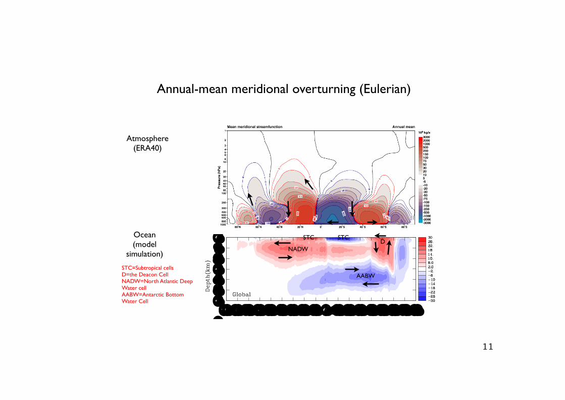
Annual-mean meridional overturning (Eulerian)

Atmosphere (ERA40)

Ocean (model

simulation)

DSTCSTC

NADW

AABW

STC=Subtropical cellsD=the Deacon CellNADW=North Atlantic Deep Water cellAABW=Antarctic Bottom Water Cell

The atmospheric meridional overturning circulation in

(moist) isentropic coordinates. (Czaja and

Marshall, 2006)

In this description, the Ferrel Cell disappears! The air flowing poleward has a higher potential temperature than that flowing equatorwards!

We will return to this issue.

11

veals (not shown) that the warm cells occupy a volumeof fluid with high stratification (thin layers) and can beidentified with the mass circulation within the venti-lated thermoclines of the Southern and NorthernHemispheres. This is further confirmed by the fact thattheir poleward extension is rather well predicted by theposition of the midlatitude zero wind stress curl lines(not shown).

The cold cells are associated with thick !O layers(weak stratification) and correspond to the circulationof North Atlantic Deep Water and Antarctic BottomWater. Note that the traditional Eulerian mass stream-function displays more modest (!10–15 Sv) cold cellmass transports.

Further information about "O is provided in Fig. 8,where the calculation was repeated separately for theIndo-Pacific (Fig. 8a) and Atlantic (Fig. 8b) basins. Asimple partitioning is thereby obtained, in which thetwo warm (symmetric) cells originate in the main fromthe Indo-Pacific basin and the (asymmetric) Northerncold cell from the Atlantic basin.

4. The partitioning of heat transport

We now combine oceanic and atmospheric massstreamfunctions within their respective potential tem-

perature layers. In so doing (Fig. 9), we have mappedthe y axis of Figs. 4 and 7 on to an energy axis, which isCA!A for the atmosphere and CO!O for the ocean.

The first striking feature of Fig. 9 is that, as antici-pated in section 2, the intensity of the oceanic cell ismuch weaker than its atmospheric counterpart (bothare annual averages, see caption of Fig. 9). Even at 20°,where "O reaches its maximum, the atmospheric masstransport is roughly 4 times that of the ocean. It is onlywithin the deep Tropics that the two transports arecomparable. This is further demonstrated in Fig. 10(continuous black curve), which shows the ratio of themaximum of "O and that of "A, computed from Fig. 9at each latitude. Note that since both "O and "A be-come small close to the equator, the mass ratio shownin Fig. 10 is rather noisy at low latitudes.

The second important feature seen in Fig. 9 is thatthe thickness of the cells in energy space is comparable.To estimate this more precisely, we have used Fig. 9and computed the change in CO!O and CA!A (hereafterdenoted as CO#!O and CA#!A, respectively) across areference contour of mass transport. The latter waschosen to be 10% of the overall maximum of "O (0.1 $32 Sv ! 3 Sv in the ocean) and "A (0.1 $ 143 Sv ! 14Sv in the atmosphere). The ratio CO#!O/CA#!A is plot-ted in Fig. 10 (gray). As one approaches the Tropics,where #!A is small, the ratio diverges. Conversely, onmoving to high latitudes where oceanic potential tem-perature variations are small (weak stratification), theratio approaches zero. In midlatitudes, CO#!O/CA#!A

FIG. 8. Same as Fig. 7 but for the (a) Indo-Pacific and (b)Atlantic basins.

FIG. 9. Annual mean atmospheric (black) and oceanic (gray)mass streamfunction within constant energy layers. The contourinterval is 10 Sv, dashed when circulating anticlockwise. The y axisis an energy coordinate (C!) in units of 104 J kg%1. The oceaniccells are the same as shown in Fig. 7 (annual mean) while theatmospheric cells are an annual-mean estimate obtained by aver-aging Figs. 4a,b.

1504 J O U R N A L O F T H E A T M O S P H E R I C S C I E N C E S VOLUME 63

12

mosphere and potential temperature referenced to thesurface for the ocean). Such a decomposition is com-monly carried out in oceanography (e.g., Talley 2003).Using Eq. (1), the ratio of atmospheric to oceanic heattransport becomes

HA

HO!

!A

!O"

CA"#A

CO"#O. #2$

In the Tropics, where transfer by quasi-two-dimensional atmospheric eddies is largely absent, Held(2001) argued that oceanic and atmospheric mass trans-ports are close to one another and set by the Ekmanmeridional mass transport. He went on to propose thatthe relative magnitude of C%& in Eq. (1) must be re-sponsible for the partitioning. To rationalize this, Heldsuggested that C%& is essentially a measure of the oce-anic and atmospheric stratification in the Tropics. Oce-anic stratification is high in the deep Tropics whereupwelling of cold fluid to the warm surface on the equa-

tor forms a pronounced thermocline. In the atmo-sphere, by contrast, tropical deep convection acts toreturn the fluid to marginal stability to moist processesin which &A, the moist static energy, has weak verticalgradients. The state of affairs is schematized in Fig. 2.Hence, as Held (2001) emphasized, dominance ofocean heat transport over atmospheric is expected inthe deep Tropics.

It is not straightforward to carry this argument tomid-to-high latitudes where it is well established thatatmospheric transient eddies cannot be ignored whenestimating meridional mass transports. Thus we mightexpect 'A and 'O to decouple moving away from theTropics, and the role of stratification in setting the par-titioning becomes much less clear.

In this paper, we attempt to estimate oceanic andatmospheric heat transports globally, motivated by thedecomposition Eq. (1). To do so, we will estimate themeridional mass transports within potential tempera-ture layers—defined by moist static energy in the at-mosphere and potential temperature in the ocean—which will allow us to estimate ' and C%& directly fromdata. Our main conclusion is that the partitioning seenin Fig. 1b can be simply understood as two limits of Eq.(2): a mass transport “' limit” in mid-to-high latitudeswhere 'A $ 'O and the atmospheric contribution toH ! HO ( HA dominates; an energy contrast “C%&limit” in the Tropics where CA&A % CO&O and wherethe oceanic contribution to H overwhelms that of theatmosphere.

The paper is set out as follows. Sections 2 and 3

FIG. 2. Schematic of the distribution of atmospheric moist po-tential temperature (&A, i.e., moist static energy) and oceanic po-tential temperature (&O) as a function of latitude and height(black contours). The equator is indicated as a vertical dashedline.

FIG. 1. (a) Estimates of oceanic (HO, gray) and atmospheric(HA, black) heat transport in PW (1 PW ! 1015 W). (b) Relativecontribution of ocean (gray) and atmosphere (black) to the totalenergy transport H ! HO ( HA using (a). Continuous curvescorrespond to NCEP-based estimates, while dashed curves corre-spond to ECMWF-based estimates. The ratios in (b) were notplotted in the deep Tropics (2°S–2°N) where HA ( HO vanishes.

MAY 2006 C Z A J A A N D M A R S H A L L 1499

13

(a) (b)

(c) (d)

Fig. 2. Configurations of the ocean basins on the aqua-planet: light grey denotes ocean,

black land. The land, when present, comprises a thin strip running in a 180! arc from pole

to pole and does not protrude into the atmosphere. Meridional gaps are introduced in the

thin strip of land in EqPas and Drake. Where there is ocean, its depth is a constant 5.2 km.

29

Ocean-planets of Enderton and Marshall. The model has a resolu-

tion of about 2.8◦ in both fluids. The simplified atmospheric physics

includes radiation, boundary layer, and convection. There is a ther-

modynamic ice model and the GM scheme is applied in the ocean.

14

The partitioning in idealized experiments

Enderton and Marshall (in press) report simulations with a coupledmodel on an ocean-covered planet. Their atmospheric model has5 vertical levels and simplified physics. They consider 4 versions ofsingle-basin geometries:Ridge has a one-grid cell land barrier connecting the poles, i.e. asingle basin with meridional boundaries. A warm climate without seaice.Drake is similar but has a circumpolar channel in the south, wherethere is sea ice.EqPas is similar but has a periodic channel in the tropics. A warmclimate without sea ice.Aqua has an ocean without meridional boundaries. Polar sea-icecaps.

15

!60 !30 0 30 60!20

!10

0

10

20

30

Aqua Surface Air Temperature

Latitude

° C

Aqua IceExtent

Aqua IceExtent

!60 !30 0 30 60!20

!10

0

10

20

30

Ridge Surface Air Temperature

Latitude

° C

!60 !30 0 30 60!20

!10

0

10

20

30

EqPas Surface Air Temperature

Latitude

° C

!60 !30 0 30 60!20

!10

0

10

20

30

Drake Surface Air Temperature

Latitude

° C

Drake IceExtent

Fig. 4. Zonal mean surface air temperature (!C) for the coupled calculations; the black

dashed line the indicated configuration and the gray lines the other configurations. Surface

air temperature in Drake is virtually identical to Ridge in the northern hemisphere and to

Aqua in the southern hemisphere.

31

16

Fig. 5. Total (top), oceanic (bottom left), and atmospheric (bottom right) heat transport

for aqua-planet configurations shown in Fig. 2. Uncertainty envelopes for observation-based

estimates of Earth’s heat transport are shown by the shaded regions (from Wunsch 2005).

32

17

Summary of results

In the simulations of Enderton and Marshall HT remains nearly con-

stant, despite drastic changes in HO and HA. Note also the compen-

sating changes in α(φ) and I(φ)!

Qualitative similar compensating transport changes have been re-

ported by Seager et al. (2002) [GCM results] and Vallis and Farneti

(2009) [idealized ocean-planet model].

Although that HT varies little in these simulations, there can be pro-

found changes of the high-latitude near surface climate: Regimes with

strong atmosphere and weak ocean transports generally have larger

sea-ice extents.18

Aqua, ! and "res

Pre

ssure

[hP

a]

0

250

500

750

1000

Depth

[m

]

Latitude

Ice Ice

!60 !30 0 30 602000

1500

1000

500

0

Ridge, ! and "res

Pre

ssure

[hP

a]

0

250

500

750

1000

300

350

400

450

Depth

[m

]

Latitude

No Ice No Ice

!60 !30 0 30 602000

1500

1000

500

0

0

10

20

30

EqPas, ! and "res

Pre

ssure

[hP

a]

0

250

500

750

1000

Depth

[m

]

Latitude

No Ice No Ice

!60 !30 0 30 602000

1500

1000

500

0

Drake, ! and "res

Pre

ssure

[hP

a]

0

250

500

750

1000

300

350

400

450

Depth

[m

]

Latitude

Ice No Ice

!60 !30 0 30 602000

1500

1000

500

0

0

10

20

30

Fig. 3. 20 year time and zonal mean potential temperature (shading) and overturning

(black contour lines). Atmosphere and ocean potential temperature contour intervals are

20 K and 2 K, respectively. The zero overturning line is bold, clockwise thin solid, and

counter-clockwise thin dashed. Overturning contours are every 10 Sv = 1010 kg s!1. Only

the top 2 km of the 5.2 km ocean are shown.

30

19

A conceptual atmosphere–ocean Hadley cell

S(y)

The Ekman-layer transports MA and MO set the meridional over-turning cell strengths. The energy transport induced by eddies andhorizontal gyre circulation is neglected. (cf. Held, 2001)

20

Ekman Transports and Overturning (775 mb); NCEP annual-mean data

!30 !20 !10 0 10 20 30!100

!75

!50

!25

0

25

50

75

100

Latitude

Tran

spor

t (Sv

)

Zonally!integrated Ekman transport

!MAMO!A

MA(y) =∮τ/f dx, and MO(y) = −

∫CO

τ/f dx; ξ ≡ −MA/MO.

21

Model assumptions

1. The strength of the meridional overturning cells set by the surfaceEkman transport.

2. The energy transport induced by eddies and horizontal gyre cir-culation is neglected.

3. The upwelling is concentrated to the equator; no interactions withthe extratropics and the deep ocean

4. The model has singular features at the equator and the polewardcell boundary.

22

Hadley Cell transports; the atmosphere

In the surface branch, EA = cAT (y) +Lvqs(y), where T (y) is the SST

and qs the surface specific humidity.

In the upper branch (assuming adiabatic ascent from the equator),

EA = cAT (0) + Lvq(0). Accordingly.

∆EA(y) = cA[T (0)− T (y)] + Lv[qs(0)− qs(y)]

For saturated conditions ∆EA ≈ cA(Γd/Γm)∆TA; where ∆TA ≡ T (0)−T (y) and Γd/Γm = 1 + Lv/cA · dq∗/dT .

23

Hadley Cell transports; the ocean

In the surface branch, EO = cOT (y).

in the thermocline branch, EO is set by the flow-weigthed surface

temperature distribution of the downwelling waters.

Calculations (Klinger and Marotzke, 2000) show that

∆EO(y) =cOMO

∫ yP

yMO

dT

dy′dy′ ≡ CO ·∆TO(y). (4)

A constant surface temperature gradient and MO ∝ (1−y/yP )b, yields

∆TO(y) = (1−y/yP )1+b yP

dTdy . For b = 1, ∆TO(0) = 0.5 · yP dTdy ; i.e. the

maximum ∆TO is half of the surface temperature range.

24

Hadley Cell transports; the partitioning

HOHA≈

cO∆TOcA(Γd/Γm)∆TA

·MO

MA. (5)

Note that MO/MA ≈ 0.8 averaged over the Tropics and

cO/[cA(Γd/Γm)] ≈ 1.3. Thus,

HO/HA ≈ TO(y)/TA(y).

Note that TA increases poleward whereas ∆TO decreases.

We now present result from calculations based on zonal-mean values

of surface temperature, specific humidity, and zonal wind stress; data

from the World Ocean Atlas 2005 and NCEP.25

!30 !20 !10 0 10 20 30

0

1

2

3

4

5

6Eneregy diff.:!T, !h/cO

Kelvi

n

Latitude!30 !20 !10 0 10 20 30!1

!0.8

!0.6

!0.4

!0.2

0

0.2

0.4

0.6

0.8

1

Latitude

Peta

Wat

t

Energy Transports

ATMOCENET

26

The Model Energy Transport; summary

1. The conceptual model gives a plausible explanation for why theocean transport exceeds the atmospheric one near the equator inthe Hadley cell.

2. However, the model under estimates the energy transports. Fromobservations HA + HO ∼ 3 PW at 15◦, whereas the model yields∼ 1 PW.

3. Energy transport induced by eddies and gyres are important, par-ticularly near the poleward cell boundary (cf. Hazeleger et al.,2004).

27

SST ( °C )

120oE 140oE 160oE 180oW 160oW 140oW 120oW 100oW 80oW 60oW

24oS

12oS

0o

12oN

24oN

18 19 20 21 22 23 24 25 26 27 28 29

28

Mid latitude transports; the atmosphere 1

Here the eddies do the transport. We assume diffusive energy trans-port (Vallis and Farneti, 2009):

v′h′ = −k∂h

∂y, (6)

where k is the eddy diffusivity; it depends on the basic state in somecomplicated fashion.

The energy transport scales roughly as

HA ∼ cA(Γd/Γm)∆TA · ρA · k ·Hd, (7)

where Hd is the density scale height and ∆TA the temperature differ-ence across the baroclinic zone. The eddy-induced mass transport isMA ∼ ρAkHd and ∆EA ∼ cA(Γd/Γm)∆TA.

29

Mid latitude transports; the atmosphere 2

The surface winds stress is approximately related to the vertically-

integrated PV flux:

τs ≈∫ρAv

′Q′ dz, (8)

where Q is the potential vorticity. Assuming diffusive PV transport

(accomplished by the same eddies that transport energy):

v′Q′ = −k∂Q

∂y∼ kβ. (9)

Thus the surface wind stress scale as τs ∼ ρAkHdβ, which implies that

MA ∼ τsβ−1. (10)

30

Mid latitude transports; atmosphere/gyres

From the Sverdrup relation, the mass transport in wind-driven ocean

gyres scale as

MO ∼ τsβ−1. (11)

Thus, the partitioning is given by

HOHA∼

cO∆TOcA(Γd/Γm)∆TA

, (12)

where ∆TO is the flow-weigthed temperature difference in the gyre.

The partitioning between the oceanic gyres and atmospheric eddies

should depend primary on the thermal contrast in the two fluids. If

τs increases, both HA and HO should increase.

31

Thermohaline circulation (THC); 1

The classical thermocline scaling predicts that MO∼∆b1/3κ2/3A2/3,

where ∆b is the buoyancy difference, κ the turbulent vertical diffusiv-

ity, and A the basin area. The rate of work performed by the turbulent

mixing:

E = ρ0

∫κN2 dz ∼ κ ·∆b.

Thus, κ∼E/∆b which yields (Nilsson and Walin, 2001)

MO ∼∆b−1/3(E ·A)2/3. (13)

For fixed E, the THC decreases with increasing ∆b! Note that ∆b=

∆bT + ∆bS; frequently ∆bS < 0.

32

Thermohaline circulation (THC); 2

Main factors that control the mixing energy E:

1) Large-scale surface winds Eτ .

2) Hurricanes EH; depends on SST, atmospheric shear, etc.

3) Tides ET , depends on basin topography and N .

HO ∼ cO∆T ·∆b−1/3(E ·A)2/3; E = Eτ + EH + ET . (14)

The THC induced heat transport is partly decoupled from the large-

scale atmosphere circulation.

Assume (incorrectly) that ∆b∼∆T , then HO∼(∆T · E ·A)2/3.

33

THC, hurricanes, and equable climates

A conceptual model of equable climates with warm poles and strong

ocean transport (Emanuel, 2002). Key elements:

1) EH∼q∗(SST )3; the mixing increases rapidly with SST

2) Also the ocean transport increases HO∼∆T2/3 · q∗(SST )2 .

3) The atmospheric circulation slows down; below a threshold deep

convection emerges in the subtropics. This moistens the clear skies

and reduces the OLR.

4) To compensate, the high latitudes warms to elevate the OLR.

Compared to the present state, the ”equable” climate has slightly

warmer Tropics but much warmer poles.

34

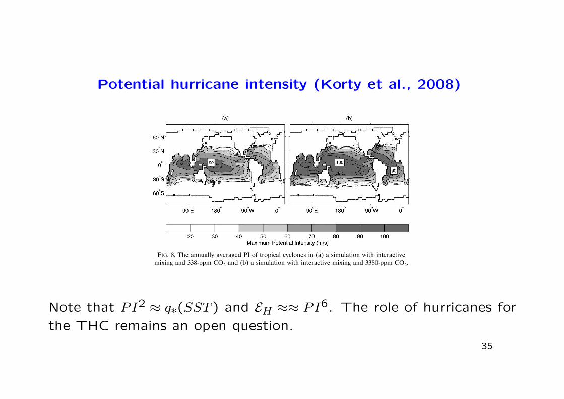
Potential hurricane intensity (Korty et al., 2008)

are considerably warmer (not shown), and the potentialintensity increases (Fig. 8), which leads to strongermixing through (8). Throughout the tropics, PI valuesare 10% (near the equator) to 40% (at the subtropicaledge) higher in Fig. 8b than in Fig. 8a; note the rapid

transition to small PI values in the subtropics of bothsimulations. The increases in PI force the values of !,via (8), to be substantially higher in the warm climatethan in the present one. Figures 9a,c,e show the totalvalue of ! in both the present climate and Figs. 9b,d,f

FIG. 9. The total value of ! (i.e., !b " !s) for (a), (c), (e) a simulation with interactive mixingand 338-ppm CO2 and (b), (d), (f) a simulation with interactive mixing and 3380-ppm CO2.Values are shown at (top) 50-, (middle) 120-, and (bottom) 220-m depth.

FIG. 8. The annually averaged PI of tropical cyclones in (a) a simulation with interactivemixing and 338-ppm CO2 and (b) a simulation with interactive mixing and 3380-ppm CO2.

648 J O U R N A L O F C L I M A T E VOLUME 21

Note that PI2 ≈ q∗(SST ) and EH ≈≈ PI6. The role of hurricanes for

the THC remains an open question.

35

Stommel and Csanady (1980)

”A relation between the T -S curve and the global heat and atmo-

spheric water transport.” The idea: HO ∼ cO∆TMO.

The oceanic freshwater transport is FO ∼ (∆S/S0)MO.

Since FO = FA, one obtains

HOLvFA

=cO∆T

Lv(∆S/S0)∼ 0.5. (15)

A caveat is that the MO carrying heat is different from the one carrying

salt.

Suppose that sea-ice transports (FI) balances FA.

(LI · FI)/(Lv · FA) = LI/Lv ≈ 0.1

36

Latitude

Dep

th (k

m)

Salinity, Atlantic 20W (LGM simulation)

!60 !40 !20 0 20 40 60

!5

!4.5

!4

!3.5

!3

!2.5

!2

!1.5

!1

!0.5

34

34.5

35

35.5

36

36.5

37

37.5

38

Sea-ice freshwater transport important in this coupled-model simula-tion (with the CCSM3)!

37

Bjeknes compensation

Bjeknes (1964) proposed that on decadal timescales anomalies in

the meridional energy transport in the ocean and the atmosphere

should be of the opposite sign, acting keep the total transport nearly

preserved.

If the storage in the ocean does not vary significantly, Bjerknes com-

pensation is expected from Stone’s steady-state argument that HTshould be fairly constant.

Let’s look at Bjerknes compensation in the idealized ocean-planet

model of Vallis and Farneti (2009):

38

16

50 100 150 200 250 300 350 400 450 500!0.015

!0.01

!0.005

0

0.005

0.01

0.015

R[OHT!AHT] = !0.14

[PW

]

[years]

OHT

AHT

PHT

0 50 100 150 200 250 300 350 400 450 500!0.05

0

0.05

R[OHT!AHT] = !0.71

[PW

]

[years]

OHT

AHT

PHT

Figure 9. Variability of the oceanic, atmospheric and planetary (i.e., total) heat transports over a 500 year period of the controlintegration, low-pass filtered to allow only decadal and longer period variability. Top and bottom panels show the transport averagedfrom 30° to 60° in the Northern and Southern hemispheres, respectively. R(OHT-AHT) refers to the correlation between theatmospheric and oceanic heat transports.

meridional overturning circulation (MOC), and it isseen from Fig. 9 that the variations in the strengthof the MOC tend to lead the variability in the oceanheat transport. Furthermore, the total heat transport(PHT in Fig. 9) is positively correlated with the oceanheat transport (OHT), implying that the atmosphereis compensating, but imperfectly, for variations in theocean transport.

Whether the atmosphere or ocean is better con-sidered to be the driver of the variability depends on

the time scale under consideration. For example, ona weekly timescale the ocean may be considered tobe steady and the variability comes almost entirelyfrom the atmosphere, whereas at longer timescalesthe ocean should be considered the controller. Fig.10 illustrates this point more graphically. The fig-ure shows the correlation between the ocean heattransport and the total transport, and the correlationbetween the atmospheric heat transport and the total,as a function of latitude and timescale. The thick

Copyright © 0000 Royal Meteorological SocietyPrepared using qjrms3.cls

Q. J. R. Meteorol. Soc. 00: 1–20 (0000)DOI: 10.1002/qj

Low-passed filtered variability of H averaged between 30N and 60N.

39

ning mean of 15 yr and weighted with the amplitude ofthe anomalies. One can see that a maximum compen-sation rate of 55% is obtained at a latitude of 70°N forthe samples with a running mean of 15 yr. The otherline in this panel shows the compensation rate for theannual heat transport estimates. Comparing these twocurves, one can clearly see that a significant increase inBjerknes compensation occurs between 50° and 80°Nby going from annual to decadal time scales.

We elucidate the above results by performing a linearregression of the divergence of the atmospheric heattransport [term on the left-hand side of Eq. (1)] ontothe flux at the atmosphere–ocean interface and onto theflux at the top of the atmosphere [both terms are on theright-hand side of Eq. (1)]. The resulting regression co-efficients are shown in Fig. 2a. Similarly we perform alinear regression of the divergence of the oceanic heattransport onto the flux at the atmosphere–ocean inter-

face and onto the time derivative of the ocean heatstorage. The resulting regression coefficients are shownin Fig. 2b. The two panels in Fig. 2 show that we ob-serve a strong compensation mechanism between 60°and 80°N. It should be noted that the variations at thetop of the atmosphere have an overall negligible influ-ence on the heat budget. However, the ocean heat stor-age still has a significant influence on the heat budgetoutside of the region between 60° and 80°N.

Figure 3 is an extension of Fig. 1a by showing corre-lation coefficients between the atmospheric and oce-anic heat transport anomalies on decadal time scales atdifferent lags in time. The time axis is such that positive(negative) times indicate that the ocean (atmosphere)leads. The anticorrelation rate in Fig. 3 is highest at70°N when the ocean leads the atmosphere by 1 yr. In

FIG. 1. (a) Correlation between atmospheric and oceanic heattransports. The solid line is calculated for samples with 15-yr run-ning mean, whereas the dashed line is calculated for samples withannual means. (b) Compensation rate of the atmospheric andoceanic heat transport anomalies for a running mean of 15 (solidline) and 1 yr (dashed line).

FIG. 2. (a) The linear regression of the divergence of the atmo-spheric heat transport onto the flux at the atmosphere–ocean in-terface (solid line) and the flux at the top of the atmosphere(dashed line). (b) The linear regression of the divergence of theoceanic heat transport onto the flux at the atmosphere–oceaninterface (solid line) and the change of the ocean heat storage(dashed line). The regression coefficients are dimensionless in thisfigure.

6026 J O U R N A L O F C L I M A T E VOLUME 20

Low-passed filtered correlation between HT and HA from Hadley Cen-

tre model (van der Swallow et al., 2007). Note the positive correla-

tions in the tropics.

40

Bjeknes compensation in the simulations

In the simulations, Bjerknes compensation occurs partly on decadal

timescales. It is the overturning ocean circulation that drives anoma-

lies in HT , to which the atmosphere compensate. In the Hadley Centre

model, changes in salinity and sea-ice cover are important dynamical

elements.

In the idealized model of Vallis and Farneti (2009), Bjerknes com-

pensation is essentially absent in the (southern) hemisphere with the

circumpolar channel.

41

18

60S 40S 20S 0 20N 40N 60N!1

!0.5

0

0.5

1

AHT!PHT

Latitude

60S 40S 20S 0 20N 40N 60N!1

!0.5

0

0.5

1

OHT!PHT

Latitude

Figure 10. Top: correlation between atmospheric energy transport and planetary (total) energy transport. Bottom: correlationbetween oceanic energy transport and planetary (total energy transport. Thick solid lines is the correlation from low-passed timeseries (a decade and longer) and the dotted lines allow successively shorter time scales to pass. The thick dashed lines use annualaveraged time series.

be the product of an appropriate circulation strength(an appropriate transport streamfunction) and a grossstatic stability. In the atmosphere the circulation iseffected by the direct, quasi-steady Hadley Cell inthe tropics and by eddy motions in mid-latitudes,and the gross static stability is roughly the averagedifference between the moist static energy betweenequatorwards and polewards flowing fluid. The oceancirculation comprises both wind-driven components —the tropical overturning cell, the classical wind-drivengyres, and a wind-driven overturning circulation —and a component dependent on a finite diapycnaldiffusivity, and its gross stability is approximatelythe potential temperature difference across a givencirculation cell, multiplied by the heat capacity.

The energy transport by the wind-driven oceanand by the atmosphere can be expected to be tightlycoupled, especially so in the tropics where the mass

transport of the Hadley Cell and the oceanic overturn-ing cells differ only by a constant factor equal to thefraction of planet’s surface covered by ocean. In mid-latitudes the coupling is somewhat less tight becauseenergy transport by the atmosphere takes place inturbulent, large-scale eddies, but nevertheless it isthose same eddies that produce the surface stress thatdrives the great ocean gyres. Theoretical argumentsthen suggest that the energy transports in the atmos-phere and wind-driven gyres ocean scale the sameway. In practice, the energy transport in the gyres isless than that in the atmosphere, both because thetemperature contrast seen by the ocean is smaller, andbecause the mass transport is smaller in the ocean’sgyres than in the atmosphere. The coupling of energytransports implies that it is difficult to change theatmospheric and wind-driven oceanic heat transportsindependently of the other and, furthermore, that

Copyright © 0000 Royal Meteorological SocietyPrepared using qjrms3.cls

Q. J. R. Meteorol. Soc. 00: 1–20 (0000)DOI: 10.1002/qj

Vallis and Farneti (2009)

Annual data

Decadal data

Correlation of H_A and H_O with H_T

Atoms.

Ocean

42