DYNAMICS OF H!GHVI A Y BRIDGES

by

J. H. Senne

and

T. K. Smith

Project HR67 of the Iowa Highway R esearch Board

Project 376-8 of the Iowa Engineering Experiment Station

August, 1961

IOWA STATE UNIVERSITY I of Science and Technology j Ames, Iowa

IOWA

ENGINEERING (ti EXPER.IMENT

STATION

2

CONTENTS

Introduction

Nature of this investigation

Definitions and notations

Definitions

Notations

History

Theoretical analysis

Load functions

Free vibration

Forced vibration

Test equipment

Test bridge

Strain measuring and recording equipment

Oscillator

Test truck

Experimental investigation

Stationary dynamic tests

~:tatic tests

Moving load tests

Determination of damping coefficient and natural frequency

Data analysis

Analysis of stationary dynamic tests

Analysis of moving load tests

Analysis to determine dynamic load distribution

Results

Recommendations for further study

References

Acknowledgments

Page

3

3

5

5

6

8

13

13

17

19

30

30

32

33

35

37

37

40

40

41

43

43

47

47

51

62

63

65

3

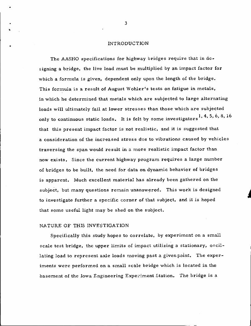
INTRODUCTION

The AASHO specifications for highway bridges require that in de-

signing a bridge, the live load must be multiplied by an impact factor for

which a formula is given, dependent only upon the length of the bridge.

This formula is a result of August Wohler's tests on fatigue in metals,

in which he determined that metals which are subjected to large alternating

loads will ultimately fail at lower stresses than those which are subjected

1 · · 1 d I · f l b . . 1, 4, 5, 6, 8, 16 on y to continuous static oa s. t 1s e t y some investigators

that this present impact factor is not realistic, and it is suggested that

a consideration of the increased stress due to vibrations caused by vehicles

traversing the span would result in a more realistic impact factor than

now exists. Since the current highway program requires a large number

of bridges to be built, the need for data on dynamic behavior of bridges

is apparent. Much excellent material has already been gathered on the

subject, but many questions remain unanaw~red, This work is designed

to investigate further a specific corner of that subject, and it is hoped

that some useful light may be shed on the subject.

NATURE OF THIS INVESTIGATION

Specifically this study hopes to correlate, by experiment on a small

scale test bridge, the upper limits of impact utilizing a stationary, oscil­

lating load to represent axle loads moving past a givenpol.nt. The exper-

iments were performed on a small scale bridge which is located in the

basement of the Iowa Engineering Expe1·:!.ment titation. The bridge is a

4

25 foot simply supported span, 10 feet wide, supported by four beams

with a composite concrete slab. It is assumed that the magnitude of the

predominant forcing function is the same as the magnitude of the dynamic

force produced by a smoothly rolling load, which has a frequency de­

te.rmined by the passage of axles. The frequency of pas sage of axles is

defined as the speed of the vehicle divided by the ax~e spacing. Factors

affecting the response of the bridge to this forcing function are the

bridge stiffness and mass, which determine the natural frequency, and

the effects of solid damping due to internal structural energy dissipation.

·• 5

DEFINITIONS AND NOTATIONS

DEFINITIONS

Impact Factor

Impact factor, as used herein, is the ratio of the difference between

the dynamic and static effect of a vehicle to the static effect. It is,

therefore, the fractional increase in the static effect of a vehicle on a

bridge due to the vehicle moving on the bridge.

Free Vibration

Free vibration is the periodic motion of an elastic system when

moving under no external forces or damping. The only forces acting

to cause the motion are the internal potential energy of the system and

the dynamic force due to the acceleration of the mass of the system.

Natural Frequency

The frequency at which an elastic system vibrates during free vibra­

tion is termed the natural frequency of the system.

Loaded Natural Frequency

The frequency at which an elastic system vibrates when loaded with

an external mass is termed the loaded natural frequency of the system.

Forcing Function

The forcing function is an externally applied, time dependent force

acting to cause motion in an elastic system.

Forced Vibration

The vibration which takes place in an elastic system when subjected

to a forcing function is termed the forced vibration of the system.

6

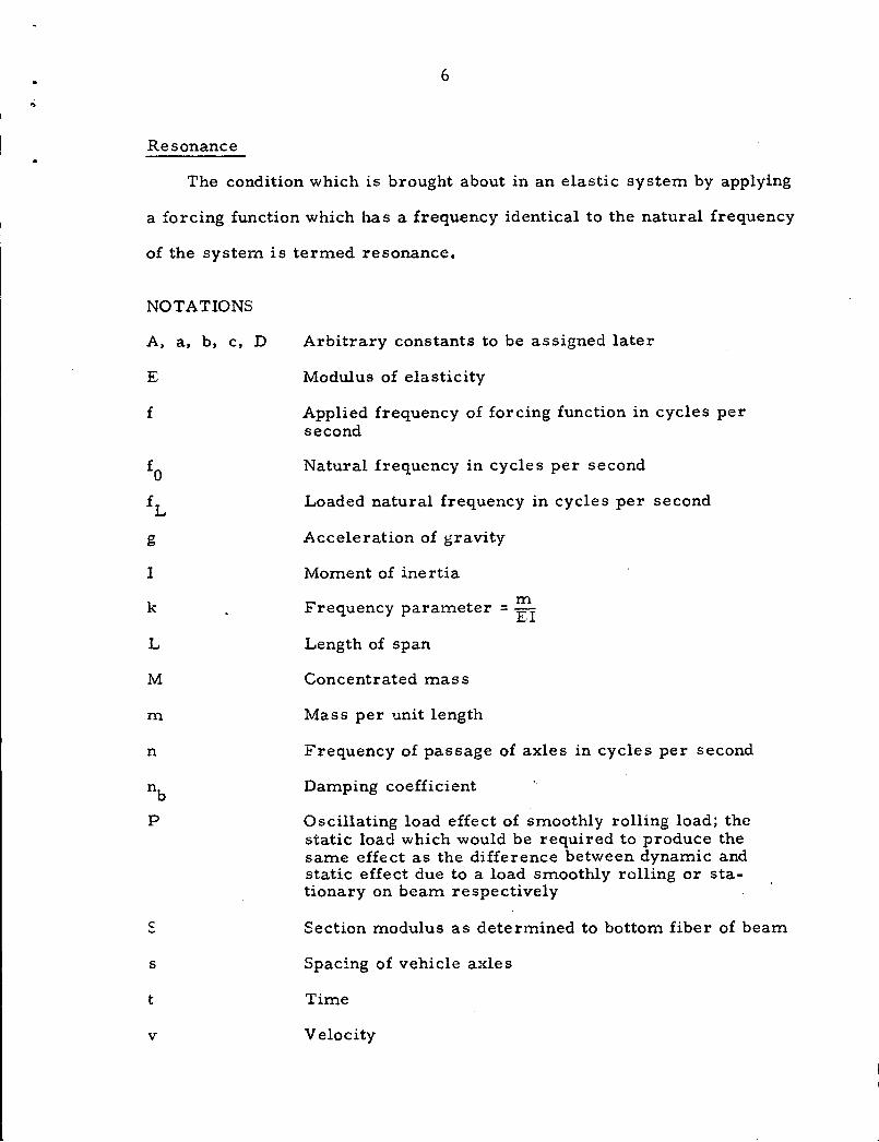
Resonance

The condition which is brought about in an elastic system by applying

a forcing function which has a frequency identical to the natural frequency

of the system is termed resonance.

NOTATIONS

A, a, b, c, D

E

f

f o

f L

g

I

k

L

M

m

n

nb

p

c ....

s

t

v

Arbitrary constants to be assigned later

Modulus of elasticity

Applied frequency of forcing function in cycles per second

Natural frequency in cycles per second

Loaded natural frequency in cycles per second

Acceleration of gravity

Moment of inertia

Frequency parameter = ~I

Length of span

Concentrated mass

Mass per unit length

Frequency of passage of axles in cycles per second

Damping coefficient

Oscillating load effect of smoothly rolling load; the static load which would be required to produce the same effect as the difference between dynamic and static effect due to a load smoothly rolling or sta­tionary on beam respectively

Section modulus as determined to bottom fiber of beam

Spacing of vehicle axles

Time

Velocity

w

\V

x

y

YD

Ys y

a

~

E

"' ct> (x, t)

7

Concentrated load

Loading function

Horizontal distance along a beam

Deflection of a beam

Dynamic deflection of a beam

Static deflection of a beam

Deflection of a concentrated mass on a beam

Acceleration

Phase angle between components of dynamic force

Unit strain

Denotes function

Function of distance and time

8

HISTORY

The problems concerned with impact due to loads traversing a

bridge primarily involve determining what time dependent forcing

functions are predominant in vibrating the structure, and what the re-

actions to these functions are. A partial list of forcing functions for

highway bridges is: (1) effects of smoothly rolling loads, (2) effects

of the spring action of a vehicle, (3) effects of rough floors or uneven

approaches causing vehicle impact on the structure, (4) effects of im-

pact caused by vertical oscillations of the bridge imparting dynamic

force to the moving mass of the load, and (5) effects of oscillations

produced by the repetition of axles across any one point. These ef-

fects or the combination of them have been investigated rather recently

b 1 . . 1, 4, 5, 6, 8, 16 I l h . l . y severa investigators • n genera t e1r cone us1ons

have agreed in considering the basis for the present AASHO specifica-

tions to be unrealistic; however, the reasons backing up these con-

clusions have not always b1Jcn in agreement. J> . .lthough these investi-

gations are of a fairly recent nature, the over-all problem of impact

stress due to moving loads started as early as the mid-19th century

when a British Royal Committee sought "to illustrate by theory C'.nd

experiment the action which takes place under varying circumstances

. . ·1 b "d .,18, p. 326 in iron rai way ri ges • A member of the committee,

Professor R. V" illis, simplified the analytic approach to the problem

by neglecting the inertia of the bridge itself. With the mathematical

assistance of another member of the committee, G. G. Stokes, Pro-

fessor Willis derived a formula for deflections due to a rolling load

.. approximated by

V z PL\1 11 + \ g 3EI/ •

9

(1)

in which the term to the right within the parenthesis is the impact factor

which is so small as to make the difference between dynamic and static

deflection negligible.

A theoretical approach considering only the mass of the bridge

was used around the turn of the century by A. N. Kryloff, and other

authors 14

• 15

have discussed the problems of an oscillating force. In

1929 H. H. Jeffcott considered both the mass of the load and bridge. His

general equation of motion was

EI a4y + m a2y = tP (x, t} - q, (x, t) a2y ax4 atl g at2 '

(2)

where q, (x, t) is the forcing function and i is the vertical position of the

load. The development of this equation marked a milestone along the

road to understanding dynamic loading, for this equation i_ncorporated all

of the more important parameters involved in the problem of forced vi-

brations in bridges. The previous attempts had made assumptions which

were not realistic.

After these earlier investigations, a very complete study was made

in which various types of forcing functions were considered in the form

of a Fourier series, and their effects were related to railway bridges.

This theoretical work, supported by experiment, gave insight into the

general problem of vibration in railway bridges.

Investigations into bridge impact were limited at first to railway

bridges. As motor vehicle transportation increased, the need for

10

similar studies in highway bridges became apparent due to the differences

in railway and highway bridges, as well as the difference in predominant

factors of _the forcing functions produced by motor vehicles and locomo­

tives passing over these bridges. The earlier investigations of railway

bridges supplied the background for the study of reactions to various

forcing functions, 'so that the main problem of the highway bridge inves-

tigator is to determine what forcing functions of motor vehicles are pre-

dominant. Since many variables contribute to the forcing function of

motor vehicles, and since these variables are not standard among different

vehicles, the task has not been an easy one.

A good collection of material on the subject of highway vibrations

can be found in the Highway Research Board Bulletin 124. In this bulletin

the effects of moving heavy loads on five simply supported bridges were

1 reported • The maximum amplitudes of vibration varied from 18 to 40

percent of the static deflections. The most important factors influencing

the vibrations of the bridge were reported as the dynamic characteristics

of the vehicle itself. The speed of the vehicle had little correlation to

the impact. Those vehicles which were spring suspended produced lower

amplitudes of vibrations than the same vehicles which were rigidly con­

nected to the axles. Scheffey10

considered the effects of three factors:

(1) smoothly rolling loads, (2) deck irregularities, and {3) repetition

of loads near resonance, as major factors in producing dynamic deflec-

tions in highway bridges~ He found that the effects of shock due to deck

irregularities were greatest for short-span bridges and decreased as

the span length increased, while the effects of repetition of loads increased

11

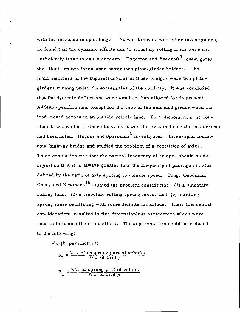
with the increase in span length. As was the case with other investigators,

he found that the dynamic effects due to smoothly rolling loads were not

sufficiently large to cause concern~ Edgerton and Beecroft 4

investigated

the effects on two three-span continuous plate-girder bridges. The

main members of the superstructures of these bridges were two plate-

girders running under the extremities of the roadway. It was concluded

that the dynamic deflections were smaller than allowed for in present

AASHO specifications except for the case of the unloaded girder when the

load moved across in an outside vehicle lane. This phenomenon, he con-

eluded, warranted further study, as it was the first instance this occurrence

had been noted. Haynes and Sparounis6

investigated a three-span contin-

uous highway bridge and studied the problem of a repetition of axles.

Their conclusion was that the natural frequency of bridges should be de-

signed so that it is always greater than the frequency of passage of axles

defined by the ratio of axle spacing to vehicle speed. Tung, Goodman,

Chen, and Newmark16

studied the problem considering: (1) a smoothly

rolling load, (2) a smoothly rolling sprung mass, and (3) a rolling

sprung mass oscillating with some definite amplitude. Their theoretical

considerations resulted in five dimensionless parameters which were

seen to influence the calculations. These parameters could be reduced

to the following:

Weight parameters:

R = Vi't. of unsprung part of vehicle 1 Wt. of bridge

R = Vvt. of sprung part of vehicle 2 Wt. of bridge

Wt of vehicle R3 = wt: of bridge

Stiffness parameter:

12

_ Fundamental period of bridge µ - Fundamental period of vehicle

Speed parameter:

_ One-half the fundamental period of bridge a - Time for vehicle to cross span

After correlating the test results to a digital computer solution of the

problem, the five parameters cited above were shown to be definitely

controlling in the dynamic variation of deflection.

Linger8 has investigated the effects of the frequency of passage

of axles from which he derived a theoretical upper limit of impact. His

experimental work checked his impact formula on two continuous bridges,

one partially continuous prestressed concrete bridge, and one simply

supported prestressed bridge. Linger was not able to investigate the

upper limits of impact due to the fact that his test vehicles could not

gain sufficient speed. The nature of his theoretical investigations, how-

ever, suggest that his forcing function can be represented by a stationary,

oscillating load. In this work this approach has been utilized in investi-

gating the upper limits of impact as derived by Linger.

13

THEORETICAL ANALYSI$

LOAD FUNCTIONS

In his treatment of loads, Inglis 7

used a Fourier series of the

form

i = CX)

w=)

h-r . i7Tx

wi smL

to represent any condition of loading. Applying the fundamental principle

of mechanics which states

d4 w = EI4,

dx

the differential equation describing any loaded beam becomes

i - CX) 4 ----

EI d y - " -:4 - / dx . 1 1 =

(3)

d2 If the boundary conditions of a simply supported beam, y and~ are

dx zero when x = 0 and L = 0, are applied, the solution takes the' form

L4 i = 00

> W. i1Tx 1

y=~ A sin-y;-• 1T EI

i = 1 1

(4)

For various loading conditions in a simply supported span Inglis

evaluated w. and demonstrated that in most cases considered the first l

term of the series gives sufficient accuracy for evaluating the load

function. Consider, for example, a load:!. distributed along the length

of the beam from x = 0 to x = L. If we consider the identity

t 0

14

. C11'X . i11'Xd 1 lL f (i-c)7rx sm -y:-s1n-y;- x= z cos L -

t 0

(i+c)7Tx cos L dx

1 fi . (i-c)7Tx 1 . (i+c)7Tx -J· = 27r l3i-c) sin L - (i+c)s1n L . '

it can be concluded that if~ is a whole number, which it is in the case of

the assumed Fourier series, then ~he above de!inite integral is zero ex-

cept for the case when i = c, in which case it is equal to

t sin 2 i7Tx dx = .!. L 2 /

L f1 2i7rxJ L - cos-y;-o

L =2·

It is therefore seen that

(Lr·~ Jo i = l

and 2 fL

wi = L lo

. i7rx l wismyl

_i

. i11'xd W Sl~ X •

L dx = T wi

dx

(5)

(6)

(7)

Consequently, using equation (7) we ca:::1 evaluate the various coefficients

w.. Where w is a uniform load from x = 0 to x = L, evaluation of the 1

various coefficients gives the following results:

w =[ Zw 1 L 11'X -, L

2w [-1-1] 4w - - cos-,,_ I = -- =-

1 L j 11' L 'iT 11' _1 0

21Tx cos­

L

15

r 0

= w 1T

[ l ·1· L ·-

w = '!::!! - ~-cos~;rx J = - ~:!: j-1-11 3 L 377 i... :,·r. - - 0 - -

4w - 31T.

The remaining coefficients can be deduced readily from the above calcu-

lations for w 1

, w 2

, and w 3

•

If we consider a uniform load on the simply supported span between

the limits x = a to x = b, and let the quantity (b-a) become infinitesimally

small, then a concentrated load W = w(b-a) will be able to be represented

by a Fourier series.

First consider the case of (b-a) equal to some definite length. It is

then apparent that

. i1Txd 2w w s1n-y:- x = i 1T

= ~w j cos i1Ta - cos iL?rb I 111' • L

L

4w r . (b )i1T . (b ) i11" I = i1T" I sin +a ZL sin -a ZL : ,

i... J

and the load distribution takes the form

i = 00

4w ' 1 . (b ) i1T . (b ) i1T . i7rx T ) rnn +a 2L sin -a 2L sm L . .,..i_=-.....1-

(8)

For the case of a concentrated load_W, ~approaches 2_ as a limit and (b-a)

approaches zero as a limit. In this case W = w{b-a). The load distribution

as taken from equation (8) becomes

or

or

i = 00

16

. i7Ta {b-a)i7T . i1Tx ~ sm L- . - ZL- sin L ,

~

4w \ {b-a)7T . i7Ta . i1Tx 1T / z'L sm L sm L ,

2W L

.:.----.--i = 1

i = 00

> i = 1

. i7Ta . i:-rx sin·-- sin--.

L L

From equation (3),

4 EI

d y _ 2w "\ ~--dx L ~/ ____

i = l

i = CX)

. i7Ta . i7TX sm-L sm-y:-.

(9)

The solution of the above equation has been demonstrated by Inglis to be

i = 00

2WL3 ~ 1 . i17a . i7Tx y = 4 L_ A sin L sm L .

EI i = l i

(10)

The validity of equation (10) can be demonstrated by comparing results

obtained from it with the known deflection of a simply supported beam

due to a concentrated load W. The central deflection of a simply supported

. WL3 beam due to a central load W is

48EI, whereas the deflection using only

the first term of equation (10) is

17

FREE VIBRATION

From d'Alembert's principle, it is known that the inertial effect

on a vibrating beam of constant cross section is ma, where~ is the

mass per unit length of the beam, and a is the downward acceleration at

any given section a distance x from the end of the beam. If gravity and

damping effects are neglected, then the equation of motion is

or

a4 EI-:--!= -ma,

ax

a4 EI~+ ma = O.

ax

2 m a4 2 a2 Letting k = EI' we have~ + k -::-l- = O.

ax at

( 11)

( 12)

Assume a solution in the form y = cp (t) sin ~, and consider the boundary

dz conditions of a simply supported beam, which are y and Y

2 equal to zero

- dx

when x = 0 and L = O. By differentiating and substituting the assumed

solution into the equation of motion, it can be seen that

4 2 'IT ,i.. (t) . 'ITX + k2 d </> (t) . 'ITX Q -:4"' sin- sin-= • L L dtz L

Therefore, cp (t) = A1

sin 27Tf0

t

if . 'IT ' 1 ) 2 /- =__,,. I_ k L~

A solution of the equation of motion is therefore

A . 1TX . 2 f y = 1 sm L sm 1T 0t,

(13)

(14)

where f0 is known as the fundamental frequency, and the right side of the

equation describes the fundamental mode of vibration. Other frequencies

18

and modes can be obtained in a similar manner by assuming solutions to

the basic equation of motion to have the form y = cp (t)sin i~x, which will

yield solutions in the form

A . i7Tx . 2. 2 f t y = 1 sm L sm i 7T 0

, ( 15)

in which the value for.!_ gives the number of the mode of vibration and the

natural frequencies for the higher modes of vibration will be i 2£0

•

If there is a mass M concentrated at a point x = a on the beam, the

natural frequency of vibration will be reduced, and this loaded natural

frequency can be computed in the following manner. A downward acceler­

d2y ation of the mass M produces a· corresponding dynamic force M - 2 .

dt According to equation (9), the primary harmonic component of this force is

2 2M d y . 7Ta . 1TX -y;- -:-z- sm L sm L ,

dt

and the basic equation of motion becomes

4 2 2 EI

a y a y ZM a y . 1Ta . 1Tx --,i- + m---..,- = -- ---.,- sin- sin- . ax'± ate. L ati::. L L

Again assuming a solution in the form y = cfi (t) sin 7Z' ,

a2y _ d<b 2(t) it is evident that a;z- - dt2

. 1/'a s1nL,

which results in EI.; <P (t) i-·rr, + lM sin2 1Tal d2

<f> (t) = o, L . L L - dtl

from which is obtained ¢ (t) = A sin 2 7T fL t

- 71"2 I EI --

and 21Tf L - :-z-v ZM . 2 7Ta L m+-sm -

L L

_ 1TZ v EIL - J!- M + 2M

G • T"1Ta I

sm L

(16)

( 17)

19

where MG repre$ents the mass of the beam. Comparing equation ( 17)

with equation (13) shows that the addition of a concentrated mass will

lower the natural frequency.

FORCED VIBRATION

The problem of bridge vibration and the impact factor derived there­

from will naturally depend on the type of forcing function. In the case of

highway bridges there are many types of forcing functions which will

cause impressed vibrations, as has been mentioned previously. In his

treatment of the subject, Linger8

has considered the effect of rolling loads

with a frequency of the repetition of axles across any given point as the

primary factor in the forcing function. Because of the limitations of speed

and axle spacing as compared with bridge length and natural frequency, the

upper limits of the theoretical impact curve could not be verified exper­

imentally. By utilizing a practical forcing function to represent the fre­

quency of passage of axles, this work possibly can shed some light on the

upper limits of impaet.

Linger suggested that a concentrated stationary, but alternating

load could be used to represent his forcing frequency of passage of axles.

To justify this substitution, it will be necessary to investigate both the

effects produced by a stationary altexnation load, and those produced by

the repetition of axle loads. In determining the effects of the alternating

load, refer to the work of Inglis, though the derivation of impact due to

a passage of axles must necessarily come from Linger, who received a

great deal of insight for his investigations from Inglis.

20

Effects of stationary alternating lo~

Given an oscillating load on a simply supported span defined by

i = 00

W_\ -;

i = l

' i11'X ' 2 ft wi sinL sm 1T J

where f is the number of oscillations per second, the differential equation

of motion, neglecting gravity and damping forces, is

4 2 i=oo

EI a y a y "' . i1rx . 2 f 74 + m ~ =) wi smL sm 1T t. Bx Bx i = I

Assuming the particular solution has the form

i = 00

,- A . i1Tx . 2 f y = ) sin L sin 1T t 1

i = l

and differentiating and substituting into the equation of motion,

or

- i 41T

4 2 2 -, A El --::-r-- - 411' f m = w. ,

L i -' 4 w.L

l

= 1T 4EI

Since from equation ( 13)

2 EI1T _ f 2 4mL4 - 0

the above can be expressed as

( 18)

or

4 w.L

A = _1 ____ 2 __

1T4EI (i

4 -~) f

0

21

A solution to the differential equation of motion becomes

i = 00 4 ~ w.L

y= L_ 1

i = 1 -1T-4E-I ~-i 4-_ -=::.:--2-) · i7Tx · 2 ft sin -r;- sin 1T • ( 19)

The complementary function, which is a part of the complete solution to

the differential equation ( 18) is the solution of the equation

4 2 EI a y +ma y

ax4 ax2 = 0 '

the solution of which has been demonstrated previously to be

A . i1TX . .2 2

£ y = sin L sin i 1T 0

t .

The complete solution of equation (18), therefore, is given by

i = co 4

) w.L

y= _i _,__

..,_i -=--1- 4Er(·4 £2

) sin iL7Tx -sin 27Tft - !..__Z sin2i 27Tf t -, •

i f 0

1T i ---z f

\ 0

-· 0 J (20)

The negative sign within the brackets was a result of satisfying the initial

conditions of y = 0 and dy = 0 when t = O. For the case of a concentrated . dt

1 d ~ir • • • 1 Z'vV . i?Ta d h d fl . oa ~ at a section x = a, w i is equiva ent to L sin L an t e e ection

due to a stationary oscillating load is given by

2WL3 y = 4

tr EI

i = 00

\ ) i = l

. i71'a , i1TX sm r:- sin r;-

. 4 £2 l - -:7

f 0

(21)

22

Moving loads of constant magnitude

The problem of moving loads has been approached by letting the

distance from the end of the beam to the load at any time be equal to:::!•

where! is the velocity of the load, and!. is the time for the load to travel

the distance 7 • Using the Fourier series, then, this load can be repre-

sented by

. i?Tvt . i?Tx i = 00

2W °"I\ T/ sm r:;- sin L"" .

""i -=._,,..l-

v If lL = f, then the load function takes the form

i = 00 2W <z: T/ ..,..i_= ____ l_

. i'l'TX . 2" ft sin -y:- sin i7T ,

and the differential equation of motion becomes

a4 a2 zw EI~+m~=-L

ax ax

i = 00

\ ~

. i?Tx . 2· f sin -y:- sin i7T t •

(22)

(23)

(24)

Using only the first harmonic component of the forcing function, recalling

equation ( 18), and considering the load to be near the center of the span,

the solution is

- [.2WL3-jl sin~ Y- 4 --~

1T EI f2

1 - -:-7 f

0

. f v or since = ZL,

. 7TX

[ 2W J sm-y:-

y = 4=: 1T EI 1 - ( ~Lf /\

\ 0

(25)

(26)

23

Practical limitations on speed suggest that the term ~Lf will be 0

very small in comparison with unity, and its square will be even smaller;

2 hence the factor 1 - (~Lf ) , for the first harmonic component of the load

\ 01

function, will be unity. To demonstrate this, consider a span of 120 feet

v 1 and a velocity of 120 feet per second (82 mph). Therefore,

2L = 2· It

would be reasonable to assume a natural frequency for a span of this length

of around 6 cycles per second. Using the above values, the value for

v 1 1 2Lf =TI' and the square of this would be 144 • This is sufficiently small

0

in comparison with unity to be disregarded. The second term within the

brackets of equation (26) is then the dynamic deflection of the bridge

centerline, and

(27)

The first term in the brackets is the static centerline deflection, which is

superimposed upon the dynamic deflection. As defined, the impact factor

of a smoothly rolling load would then be ;Lf • Since the rolling load of 0

constant magnitude increases the deflection of the beam over the same

static load, this impact factor, ~Lf , which is associated with a smoothly 0

rolling load, can be equated to the ratio of a load P divided by the station-

ary load"'!!._, where P is defined as the oscillating load effect of a smoothly

rolling load. P is, therefore, equivalent to the static load which, when

placed at the center of the span, would be required to produce the same

deflection as the maximum dynamic component of a smoothly rolling

load W. Hence

v p ~=w.

0

:i<.:ffect of the passage of axles

24

(28)

Given a spacing between axles of..'.:• and a vehicle speed!• the fre­

quency representing the passage of axles over any given spot is

v n=-. s (29)

The forcing function representing the repetition of axles is

P sin 27Tnt • (30)

If the damping effect is taken to be 47Tnbm ~i and the effect of the mass of

the vehicle is taken into consideration as a part of the forcing function

a2-equa1 to - M d sin 7Z', the differential equation of motion will be

at

82 l Psin27Tnt - M-:-i-

at ..... ....J

• 1TX sin -T- ,

L (31)

where y is the vertical deflection of the mass of the load. As with previous

solutions, that for equation 31 will take the form

y = cf> (t) sin 7Z' . (32)

Considering that the forcing function is equivalent to a stationary vibrating

load, y is a function of time only. Hence

y=</>(t). (33)

Differentiating equations {32) and {33) and applying to equation (31),

4 EI7T ,1, (t} + 4 7T d cfl (t) 4"' nbm dt

L + d 2 ¢ (t) _ 2P . 2 t 2M d 2

ct> (t) m z - L sin 7Tn - L 2 ,

dt dt (34)

EIL1T4

<P (t) + 47Tn Lmd ¢ (t) + rlLm + 2M] d2

cf> (t) = 2Psin27Tnt, L

4 b dt .. z dt

or

25

or ~ r1 2Ml cJ> (t) + 41Tnb [·1 ZM··1 mL I 1 + lm 1 + lm I

l.. - -I

d</>(t) d2

cJ>(t) + --:......:....:. dt dt2

2P = mL+ZM sin21Tnt. (35)

Referring to equations (13) and (14), and putting this load near the center

of the bridge so that a = ~ ,

f 2 L __ 1_..._....-----...--- = _1_._,...,. -f 2 -

1 ZM . 2 ?Ta

1 ZM •

0 +rm sm L +Im

(36)

Also from (13)

4 411' = 4 2£ 2 • mL 4 11' o

(37)

Applying equations (36) and (37) to equation (35) and rearranging,

I 2) dz </J (t) fL d </> (t) 2 2 2P . dtz + 4ir"b (£T dt + 4ir fL ~ (t) = mL+lM sm lirnt. (38)

0 .

According to Linger, the particular solution to equation (38) is of the

form

cf> (t) = A sin21Tnt + B cos 211'nt • (39)

Differentiating equation (39) and substituting into equation (38)

(40)

and (41)

26

from which

and

2P A= 2 l

(mL+2M)411 f L

0 B _ 2P

- -(m_L_+-2M-) 4_11_,,2 ..... fL-z- ~-:; ) 2 (4nb2n2

). 1 - -:-z + -4..---

f f . L o .

Utilizing the trigonometric identity

A sin21Tnt + 2 cos 21Tnt = D(sin 211nt - 13 ).

in which

I 2 2 D =\/A + B and

B tan 13 = A ,

it can be determined that the particular solution to equation (38) is

2P sin (21Tnt - 13) sin T

y =-----.....--1 (mL+2M) 41T

4£L

2

(42)

(43)

(44)

(45)

Recalling equations (36) and (37), the first term on the right hand side of

equation (45) can be put into a more convenient form as follows:

2P ~L_\ 2P 1W) 2WL3

P (mL+2M) 41T 4£L 2 \mLJ = 4112mL£0 2 l.w = 1T 4EI w . (46)

Therefore,

27

2WL3 P y. = --..--

1 7T4EI W

sin (27Tnt - ()} sin 7Z' (47)

(;2 2) 2 + CY2) 'L· \o

1 +

This equation is only the particular solution to the original differ-

ential equation (38). The complementary solution must be added to equation

(4 7) to arrive at the complete solution. According to Linger, the general

form of the complementary solution has the form

where f L is the loaded damped frequency and b

f = \ Ii -"bfL j . Lb \/ £2

. 7TX smL

(48)

The proper boundary conditions are y = 0 and dy = 0 when t = O, and dt

the complete solution is then

where

f 2 L

q = 2 7Tnb -::-z- t • £

0

sin (27Tnt-!3}-e-q ~ sin27TfL t L b • 7T'X s1n-y; ,

I (49)

_I

The complementary solution is a function of damping, and it will be-

come0insignificant as the load traverses the bridge in such a way that the

28

:ratio of successive amplitudes will be

e -21Tnb [fLYfo 2 J. In the case of a load traversing a bridge, Linger has shown that the fre-

quency of the bridge is that of the particular solution by the time the load

has reached the center of the bridge; hence, for the purposes of this in-

vestigation the complementary solution is insignificant and can be dis-

regarded. In representing successive moving loads by a stationary

oscillating load, the complementary solution will cease to be effective at

the time a steady state oscillation is reached; and it can again be disre-

garded. The effective deflection due to passage of axles is then defined

by the particular solution, or equation (47). The maximum value of this

deflection, assuming that the frequency of passage of axles coincides with

the frequency due to the moving load effect, and that they are in phase,

is given by

2WL3 y - -----

- 11' 4EI

p w·

(50}

For moving loads Linger has replaced the quar..tity -~ by its equivalent

v ZLr and, dividing by the static deflection, arrived at the impact factor of 0

· IF=

v 2Lf

0

{,~ 2 2 (2 2

-\ I i - ~) + ~)\. ! f 2 \ f

I L \ 0 ' .

(51)

29

Since the object of this investigation is to examine and correlate the upper

limits of this theoretical impact factor to actual tests, the expression will

be more useful using ~instead of ~Lf • Not all of the variables in equa­o

tion (51) are independent when the effect of passage of axles is obtained

with a stationary oscillating load. Since ;Lf =.;. and n = :, determin­o

ation of s and.! will necessarily cause~ and the ratio ~r or ;Lf to be 0

known for any given bridge. The assumptions used throughout the deriva-

tions considered the deflection to be on the lateral centerline of the span

when the load is at the center. These assumptions are valid and are the

critical conditions in a simply supported span.

30

TEST EQUIPMENT

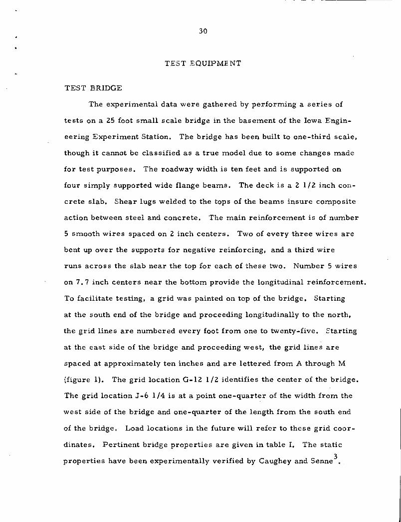
TEST BRIDGE

The experimental data were gathered by performing a series of

tests on a 25 foot small scale bridge in the basement of the Iowa Engin­

eering Experiment Station. The bridge has been built to one-third scale,

though it cannot be classified as a true model due to some changes made

for test purposes. The roadway width is ten feet and is supported on

four simply supported wide flange beams. The deck is a 2 l /2 inch con­

crete slab. Shear lugs welded to the tops of the beams insure composite

action between steel and concrete. The main reinforcement is of number

5 smooth wires spaced on 2 inch centers. Two of every three wires are

bent up over the supports for negative reinforcing, and a third wire

runs across the slab near the top for each of these two. Number 5 wires

on 7. 7 inch centers near the bottom provide the longitudinal reinforcement.

To facilitate testing, a grid was painted on top of the bridge. Starting

at the south end of the bridge and proceeding longitudinally to the north,

the grid lines are numbered every foot from one to twenty-five. .Starting

at the east side of the bridge and proceeding west, the grid lines are

spaced at approximately ten inches and are lettered from A through M

{figure 1). The grid location G-12 l /2 identifies the center of the bridge.

The grid location J-6 l /4 is at a point one-quarter of the width from the

west side of the bridge and one-quarter of the length from the south end

of the bridge. Load locations in the future will refer to these grid coor­

dinates. Pertinent bridge properties are given in table I. The static

properties have been experimentally verified by Caughey and Senne 3

•.

12 Divisions at 1011

each = Io'- 011

a b c d f g h k m

PECIAL 2 6" [ 8.2 lb BEAM 4

BEAM I 12 B 22 BEAM 3 3'- 2 5/811

TYPICAL SECTION OF BRIDGE

m

k

Chart jno. 2 Chart no. I

~ -- -- J ·--i--

I n- _g-1 I

I - I I I

-12 B 16 1/2 Sp.

00 ;::: h

g I'-

f

I I

n-'? _1.J ..=.'/ -- - - -

I

2 B 22

NORTH ~-1. -(j) e

d ,, ~ ~-- I -

12 B 22

c I

b ~---,a-

I I I

~ ,.._

I I ~14 -

g-4 - -1--, - I I - ~--

0 I 2 3 4 5 t 7 8 9 10 11 12 13 .14 15 16 17 18 19 20 21 22 23 24 5

I -I - II

12 B 16 1/2 Sp.

25 0 g- gage

BRIDGE LAYOUT with GRID SYSTEM

Figure 1. Test bridge.

32

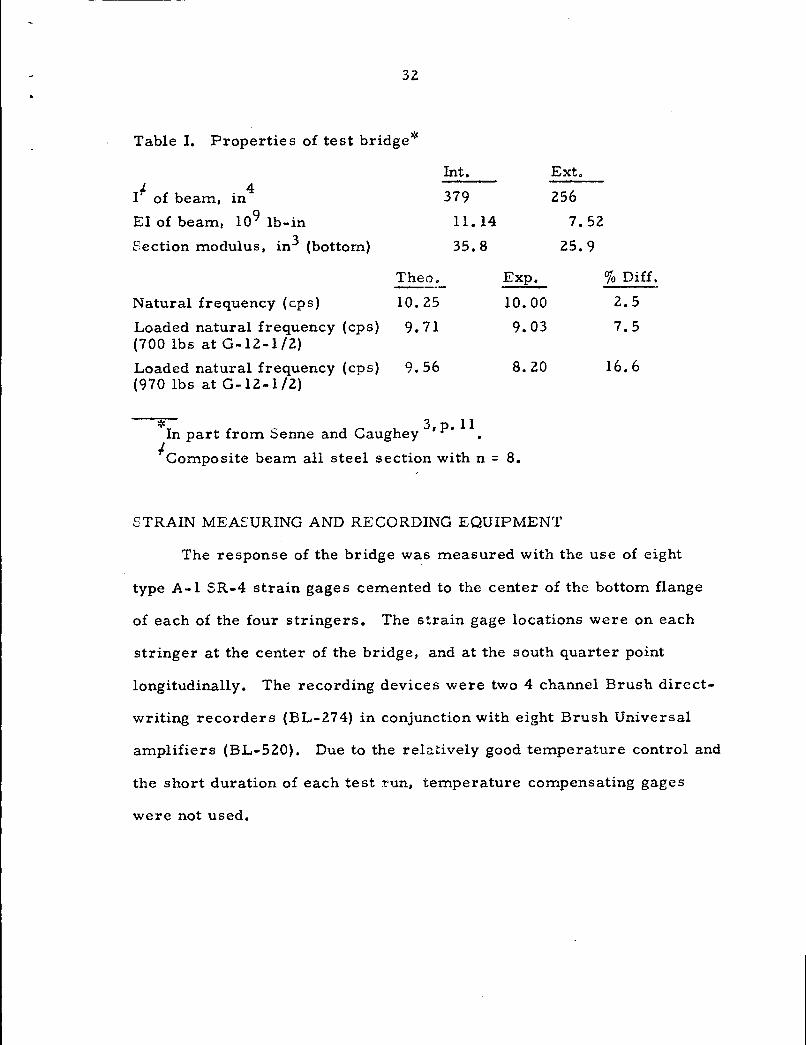
Table I. Properties of test bridge*

I/. of beam, in 4

EI of beam, 109 lb-in

Section modulus, in3 (bottom)

Natural frequency (cps)

Loaded natural frequency (cps) (700 lbs at G-12-1/2)

Loaded natural frequency (cps) (970 lbs at G-12-1/2)

Theo.

10.25

9.71

9.56

Int.

379

11. 14

35.8

* - 3 p. 11 In part from ::>enne and Caughey ' I

Exp.

10.00

9.03

8.20

r Composite beam all steel section with n = 8.

Ext.

256

7.52

25.9

STRAIN MEAEURING AND RECORDING EQUIPMENT

% DifL

2.5

7.5

16.6

The response of the bridge was measured with the use of eight

type A-1 SR-4 strain gages cemented to the center of the bottom flange

of each of the four stringers. The strain gage locations were on each

stringer at the center of the bridge, and at the south quarter point

longitudinally. The recording devices were two 4 channel Brush direct-

writing recorders (BL-274) in conjunction with eight Brush Universal

amplifiers (BL-520). Due to the relatively good temperature control and

the short duration of each test run, temperature compensating gages

were not used.

33

OSCILLATOR

The apparatus used to produce the stationary oscillating loads on

the bridge was a rotating eccentric weight device (figure 2). The force,

F, in pounds produced by such a rotating weight in any one direction is

given by the equation,

F 2 . = mew s1nc.u t,

where m is the mass of the eccentric weight in pounds mass, ~ is the ec-

centricity of the center of the eccentric mass in feet, ~ is the rotational

velocity in radians per second, and.!_ is the time in seconds. The device

was constructed so that two equal eccentric masses rotated with the same

frequency in the same plane, but in opposite directions, in phase ver-

tically, but 180 degrees out of phase horizontally, so that the horizontal

component of the oscillating force was canceled and the vertical com-

ponent was reinforced. The device was operated by a one horsepower

variable speed motor. The eccentric weights were threaded on shafts

so that their eccentricity could be varied at will, and were provided with

locking screws so that they would not slip during operation. A curve

was drawn, relating mass eccentricity and 'rotational frequency for a con-

stant oscillating force. This enabled the oscillator to be operated at

various frequencies while maintaining a constant force. The speed of

the oscillator was controlled by so adjusting the variable speed control

on the motor as to make a radially drawn chalk line on the oscillator

drive pulley appear stationary when an electronic strobotac, set to the

proper frequency, was focused on the chalk line. A permanent record

and check on this frequency was obtained by operating an event marker

on the oscillograph by a set of contact points, which in turn were operated

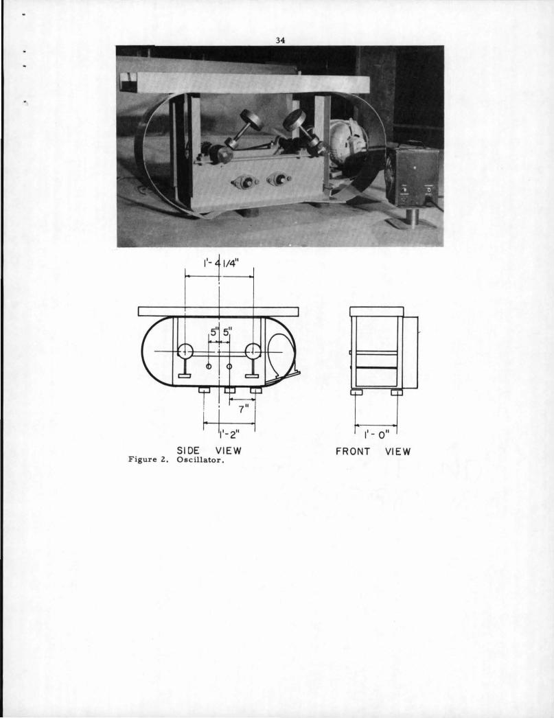
34

I

i.:.J c:~

7"

1'-211 I - II 0

SIDE VIEW FRONT VIEW Figure 2. Oscillator.

•.

35

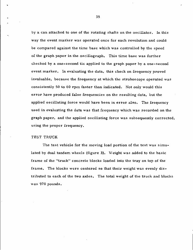
by a can attached to one of the rotating shafts on the oscillator. In this

way the event marker was operated once for each revolution and could

be compared against the time base which was controlled by the speed

of the graph paper in the oscillograph. This time base was further

checked by a one-second tic applied to the graph paper by a one-second

event marker. In evaluating the data, this check on frequency proved

invaluable, because the frequency at which the stroboscope operated was

consistently 50 to 60 rpm faster than indicated. Not only would this

error have produced false frequencies on the resulting data, but the

applied oscillating force would have been in error also. The frequency

used in evaluating the data was that frequency which was recorded on the

graph paper, and the applied oscillating force was subsequently corrected,

using the proper frequency.

TEST TRUCK

The test vehicle for the moving load portion of the test was simu­

lated by dual tandem wheels (figure 3). Weight was added to the basic

frame of the "truck" concrete blocks loaded into the tray on top of the

frame. The blocks were centered so that their weight was evenly dis­

tributed to each of the two axles. The total weight of the truck and blocks

was 970 pounds.

•

SIDE VIEW

Figure 3. Test vehicle .

2'-112"

FRONT VIEW

37

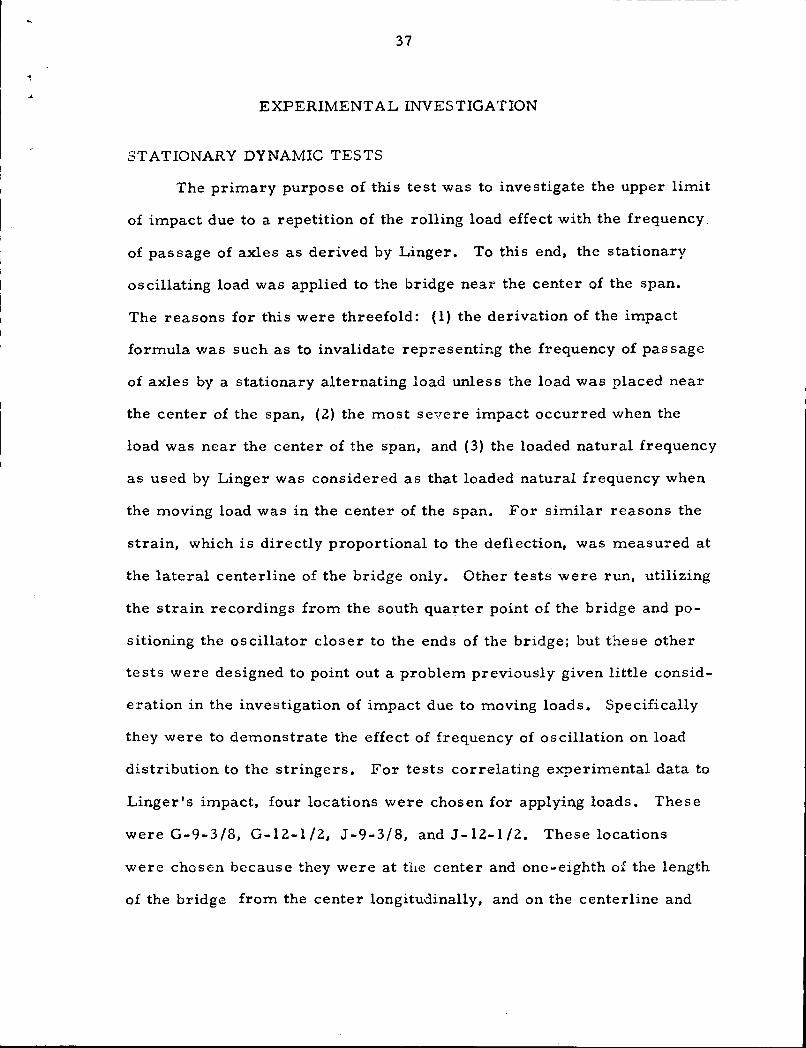
EXPERIMENTAL INVESTIGATION

STATIONARY DYNAMIC TESTS

The primary purpose of this test was to investigate the upper limit

of impact due to a repetition of the rolling load effect with the frequency

of passage of axles as derived by Linger. To this end, the stationary

oscillating load was applied to the bridge near the center of the span.

The reasons for this were threefold: (1) the derivation of the impact

formula was such as to invalidate representing the frequency of pas sage

of axles by a stationary alternating load unless the load was placed near

the center of the span, (2) the most se~rere impact occurred when the

load was near the center of the span, and (3) the loaded natural frequency

as used by Linger was considered as that loaded natural frequency when

the moving load was in the center of the span. For similar reasons the

strain, which is directly proportional to the deflection, was measured at

the lateral centerline of the bridge only. Other tests were run, utilizing

the strain recordings from the south quarter point of the bridge and po­

sitioning the oscillator closer to the ends of the bridge; but these other

tests were designed to point out a problem previously given little consid­

eration in the investigation of impact due to moving loads. Specifically

they were to demonstrate the effect of frequency of oscillation on load

distribution to the stringers. For tests correlating experimental data to

Linger's impact, four locations were chosen for applying loads. These

were G-9-3/8, G-12-1/2, J-9-3/8, and J-12-1/2. These locations

were chosen because they were at the center and one-eighth of the length

of the bridge from the center longitudinally, and on the centerline and

38

one-quarter of the width from the centerline laterally. Due to a slight

camber of the bridge the oscillator could not be set flat on the slab and

still be stable. For this reason the oscillator was set up on three

supports which made the oscillator stable at all times (figure 2). The

position of the three supports was determined by operating the oscillator

in various positions under the device. Due to the unbalance of the motor

on one side, the best dynamic results were gained from placing the

supports in this position. This had the effect of concentrating the load

on three supports instead of over the area of the oscillator base, which

in fact was more in keeping with the theoretical considerations. It

made the problem of placing the load at exactly the grid location desired

much more difficult, but this was not a serious problem because the

test was designed to compare oscillatory load effects with static load

effects. To this end it was sufficient to insure that the oscillator was

set at the same spot for both the static and dynamic tests.

The dynamic tests were conducted by varying the frequencies of

oscillation while maintaining the same applied force. Since the most im­

portant effects, those which would approach the upper limits of impact,

would be gained by applying frequenc~es near the loaded natural frequency;

the range of frequencies including the loaded natural frequency was always

investigated. The weight of the oscillator was 700 pounds, and the dy­

namic force which was applied by the oscillator was designed to be 70

pounds. As has been mentioned, the oscillator frequency was generally

greater than was intended, but the transmitted force was adjusted ac­

cordingly.

' 39

'

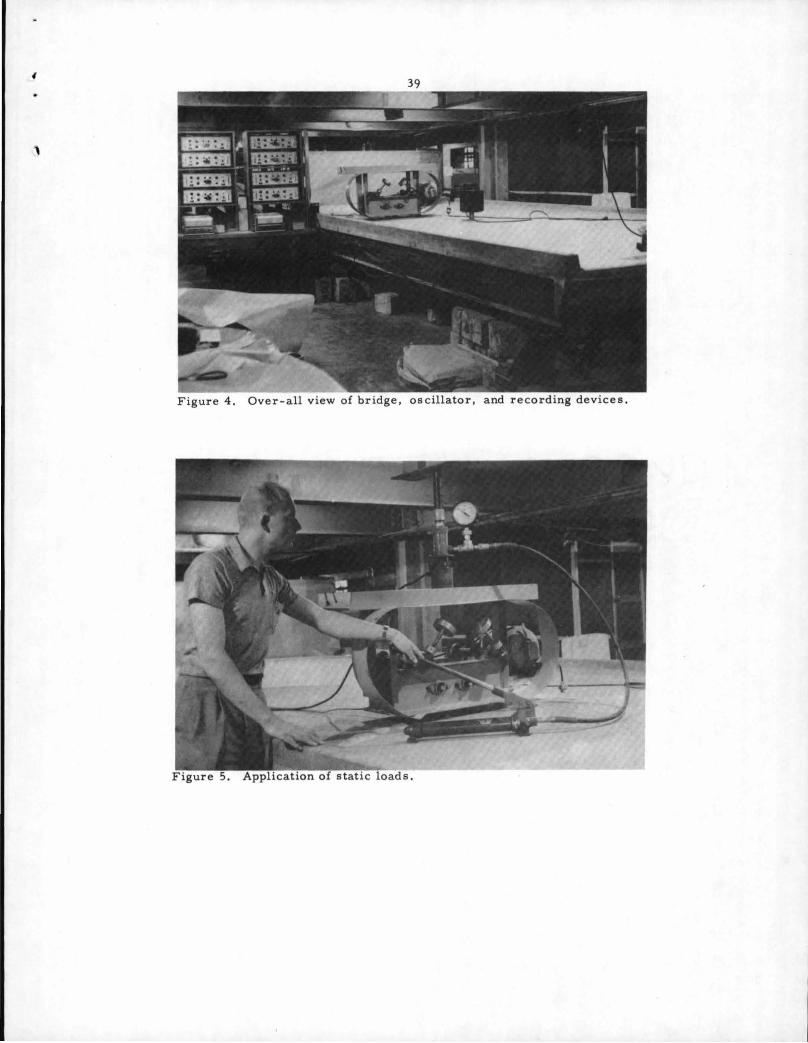
Figure 4. Over-all view of bridge , oscillator, and recording devices.

40

STATIC TESTS

The static load was applied to the oscillator at rest by means of

an hydraulic jack (figure 5). The jacking was done against wide flange

beams supporting. the floor above. A Baldwin SR-4 load cell which had

been calibrated previously was placed between the jack and the oscillator

to determine the static load applied. Large static loads were applied so

that the readings on the Brush recorders would not be unduly affected by

temperature changes throughout the loading time. This was necessitated

because of the lack of temperature compensating gages. After each load

test the applied load was returned to the value of the initial load, and

the strain readings were effectively returned to zero. A load-strain

diagram was then drawn for each stringer from data thus obtained.

MOVING LOAD TESTS

There was difficulty in trying to propel the simulated "trucks"

across the bridge and perform moving vehicle tests on the test bridge due

to crowded conditions. Since there were no roadways leading off the

bridge, it was necessary to stop the vehicle abruptly. Fortunately there

was a ten-foot bridge built at the north end of the 25-foot bridge which

was sufficient to enable the "truck" to be pushed onto the test bridge.

The relatively short distance traversed by the "truck" enabled this initial

velocity to be sustained until it was abruptly stopped by ropes attached

to the 11truck 11 and the ceiling beams near the north end of the bridge.

The velocity of the "truck" was measured by a photoelectric cell at mid­

span. A four-foot shield which interrupted a beam of light to the photo­

electric cell was attached to the "truck". The photoelectric cell operated

41

a relay which in turn operated an event marker on the oscillograph.

The velocity of the vehicle could then be determined by dividing four

feet by the time in seconds that the event marker was engaged. The

speed of the vehicle was determined in this manner. In all moving load

tests, the vehicle was directed along the center of the bridge.

Since the speed of the test vehicle could not be varied greatly be-

cause only human motive forces were used, the more important results

of the moving load tests were looked for in the area of impact due to

obstructions on the test bridge. For this phase of the tests, a piece of

angle iron giving a one-quarter inch vertical obstruction was placed at

various locations on the span to give an idea of the size of impact due to

uneven approaches or obstructions on the bridge floor.

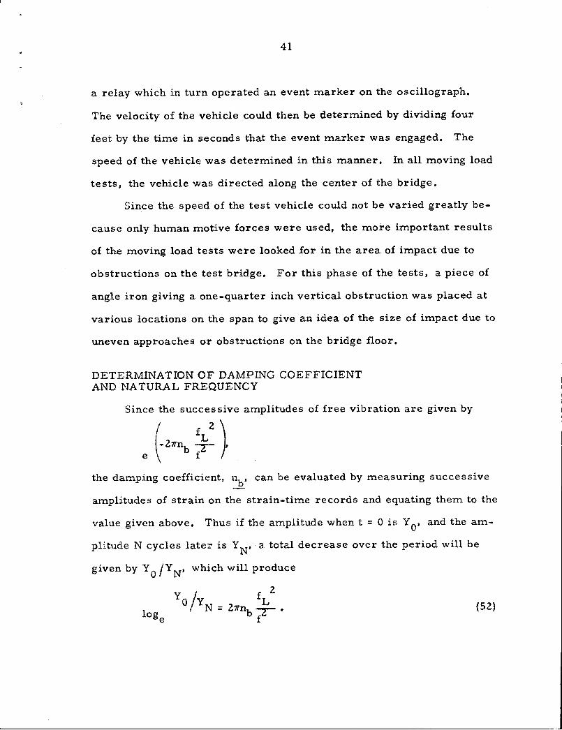
DETERMINATION OF DAMPING COEFFICIENT AND NATURAL FREQUENCY

Since the successive amplitudes of free vibration are given by

e (-z~~ :~z) the damping coefficient, nb, can be evaluated by measuring successive

amplitudes of strain on the strain-time records and equating them to the

value given above. Thus if the amplitude when t = 0 is Y 0

, and the am­

plitude N cycles later is Y N' a total decrease over the period will be

given by Y 0

/Y N' which will produce

log e

Y0/1Y fL

2

. N = 21Tnb ~. f

(52)

42

The average decrement. which is commonly known as the average log-

rithmic decrement is then given by

2 1 y I fL W loge o y n = 21T~ T •

Since the damping coefficient was evaluated from strain records com-

piled when the bridge was vibrating freely and without a load. fL = f,

hence

The value found for this bridge was nb = O. 0131, which becomes negligible

for any consideration in evaluating test results. The method employed

in obtaining free vibrations in the bridge structure was to suspend a

person from the stringers of the floor above the bridge. This person

would then set the bridge in oscillation by striking it with his feet, and

immediately lift himself off the bridge. The strain records from these

tests were also used in determining the various loaded natural frequencies

as well as the natural frequency of vibration and damping coefficient.

-,

43

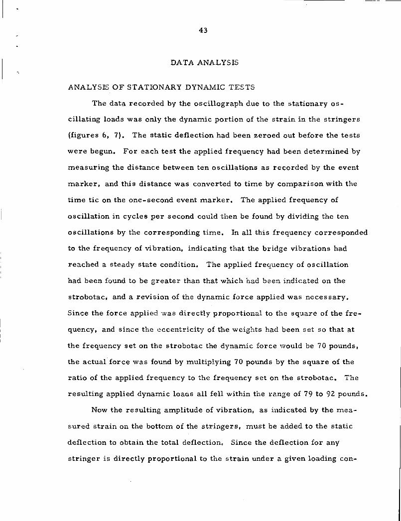
DATA ANALYSIS

ANALYSIS OF STATIONARY DYNAMIC TESTS

The data recorded by the oscillograph due to the stationary os­

cillating loads was only the dynamic portion of the strain in the stringers

(figures 6, 7). The static deflection had been zeroed out before the tests

were begun. For each test the applied frequency had been determined by

measuring the distance between ten oscillations as recorded by the event

marker, and this distance was converted to time by comparison with the

time tic on the one-second event marker. The applied frequency of

oscillation in cycles per second could then be found by dividing the ten

oscillations by the corresponding time. In all this frequency corresponded

to the frequency of vibration, indicating that the bridge vibrations had

reached a steady state condition. The applied frequency of oscillation

had been found to be greater than that which had b·~en indicated on the

strobotac, and a revision of the dynamic force applied was necessary.

Since the force applied was directly proportional to the square of the fre­

quency, and since the eccentricity of the weights had been set so that at

the frequency set on the strobotac the dynamic force would be 70 pounds,

the actual force was found by multiplying 70 pounds by the square of the

ratio of the applied frequency to the frequency set on the strobotac. The

resulting applied dynamic loacis all fell within the range of 79 to 92 pounds.

Now the resulting amplitude of vibration, as indicated by the mea­

sured strain on the bottom of the stringers, must be added to the static

deflection to obtain the total deflection. Since the deflection for any

stringer is directly proportional to the strain under a given loading con-

____ --~"""'O ... ne..,,.. second ·~=e:..-:.,_,,.,......,. _,.___~,__-_._ ~ ~ T

uency at maximum

CHART NO RA-2'141 30 ·~NBTJl,WIMENTB

Vehicle location, trac_e_J Figure 6. Typical oscillating load strain-time record.

One. se.cond time trace~ Time i_d

Figure 7. Typical moving load strain-time record.

1.4

1.2

1.0

0.8

Impact

0.6

0.4

0.2

0

- Theoretical o Expermental

total moment Axle spacing= 8.34ft.

0 0

0

01---~~~--'-~~~~-'-~~~~~~~~----'

60 70 80 90 Velocity, ft. /sec.

Figure 8. Results of stationary dynamic tests considering total moment.

100

45

dition, the following analysis will be in terms of deflection, although the

actual measured quantity is strain. Only half the amp!itude of the dynamic

deflection can be properly added to the static deflec';ion, because during

half the period of vibration the beam is subjected to negative moment;

that is, it is concave downward. For this reason the half 2.v.plitude of

vibration was divided by the corrected appl.ieC. dynamic lead to give a dy-

namic deflection per unit load, which will be called Yn. It is valid to ex­

press the dynamic deflection in terms of u!lit load, be(;ause in vibration

analysis all other factors being equal, the deflectim·1 o.f an elastic system

is directly proportional to the applied dynamic force. This is stated

mathematically by equation (45). From the static load tests a similar

deflection per unit load was obtained and this deflection will be called

y 5 • The total deflection, y T' of any one stringer is then given by the sum

(53)

Since this impact factor was defined as

(54)

it can be seen that the measured unit impact factor, due to unit loads can

Yn be expressed as - • This unit impact factor must be corrected for the

Ys

assumed loads applied by any theoretical axle spacing and speed, however,

to be compared with the impact equation derived by Linger. Since the

force causing the dynamic part of the deflection is assumed to be caused

by P, as given by equation (30), the total dynamic deflection is given by

PyD. The total static deflection is likewise caused by the weight of the

..

46

load W, and is given by the quantity vVy c • The actual measured imj:>act

factor is then given by the quantity

p Yn w· Ys

...,

(55)

and the correction factor for obtaining the impact factor is seen to be

P h. h · · 1 t v s· th · .,,- f · W , w ic is equ1va en to ZLf • ince e quantity t.d_, 0

:i..s a cor..stant 0

for any given bridge, the correction factor is a functicm of t~-:.e vehicle

speed.

second.

The value of 2Lf for this test bridge in see::: co be 500 feet per 0

These tests were performed with a station'.l:..·7 load, end a con-

cept of velocity seems at first glance to be sadly lacki::ig. If a theoretical

axle spacing is chosen, an associated velocity is forthcoming from equation

(29) so that

V = sn • - (56)

For this test then, fictitional axle spacings were chosen so that when

multiplied by the applied frequency for any test run, a corresponding

velocity was obtained. Axle spacings were chosen in such a way that the

quantity ~Lf would always be small, and the value for W would always 0

be 700 pounds. In this way the loaded natural frequency would be correct

for the actual load of the vibrator. In light of the considerations, the ex-

perimental impact factors were then determined by multiplying the unit

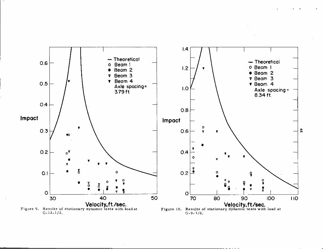
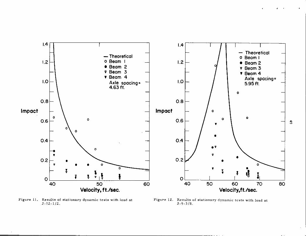
Yn b . f . sn R impact, - ' y a correction actor, soo· esults are compared between Ys

this impact factor and the theoretical curve for various axle spacings

(figures 9-12).

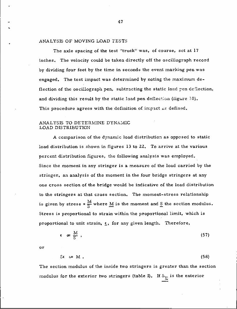
.. 47

ANALYSIS OF MOVING LOAD TESTS

The axle spacing of the test 11truck11 was, of course, set at 17

inches. The velocity could be taken directly off the oscillograph record

by dividing four feet by the time in seconds the event marking pen was

engaged. The test impact was determined by noting the maximum de-

flection of the os cillograph pen, subtracting the static loc..d pen deflection,

and dividing this result by the static load pen deflect;_on (figure J.O).

This procedure agrees with the definition of irr..p1ct c.i.f2 defined.

ANALYSIS TO DETERMINE DYNAMIC LOAD DISTRIBUTION

A comparison of the dynamic load distributio::-i as opposed to static

load distribution is shown in figures 13 to 22. To arrive at the various

percent distribution figures, the following analysis was employed.

Since the moment in any stringer is a measure of the load carried by the

stringer, an analysis of the moment in the four bridge stringers at any

one cross section of the bridge would be indicative of the load distribution

to the stringers at that cross section. The moment-stress relationship

is given by stress =~where Mis the moment and~ the section modulus.

Stress is proportional to strain within the proportional limit, which is

proportional to unit strain, !_, for any given length. Therefore,

E (57)

or

Se u= M • (58)

The section modulus of the inside two stringers is greater than the section

modulus for the exterior two stringers {table I). If SE is the exterior

0.6

0.5

0.4

Impact

• 0.3

0.2 ov

• • v

0.1 • g

• v 0

•

•

8 •

•

- Theoretical o Beam I • Beam 2 v Beam 3 • Beam 4

Axle spacing= 379 ft.

0

0 • 0

• i •

I

I I

1.4

1.2 •

1.0

0.8

Impact 0

0.6 v

• • 0.4 0 v

v 0.2 • 0

•

• •

vv

~~ ~

- Theoretical o Beam I • Beam 2 v Beam 3 • Beam 4

0 • • v

Axle spacing= 8.34 ft.

0

• • • v v v OJ__~~~~~~~~-'-~~~--=--~~~~~~ O~~~~~~~~~~~~~~~~~~~~

30 40 50 70 80 90 100 110 Velocity, ft/sec. Velocity, ft/sec.

Figure 9. Results of stationary dynamic tests with load at Figure 10. Results of stationary dynamic tests with load at G-12-1/2. G-9-3/8. .

~ 00

1.4

- Theoretical 1.2 o Beam I

•Beam 2 v Beam 3 • Beam 4

1.0 Axle spacing= 4.63 ft.

0.8

Impact 0

0 0.6

0.4

0

0.2 • v • • •

' v I i ' v v t o,__ ________ __,_ ___ __:_ ____ ____.

40 50 Velocity, ft. /sec.

Figure 11. Results of stationary dynamic tests with load at J-12-1/2.

60

1.4

1.2

1.0

0.8

Impact

0.6

0.4

0.2

0

v •

- Theoretical o Beam I • Beam 2 v Beam 3 •Beam 4

Axle spacing= 5.95 ft.

0

0

• i 0 ,__ ___ ___,_ ____ __J_ ____ __J__ ___ ----'

40 50 60 70 Velocity, ft. /sec.

Figure 12. Results of stationary dynamic tests with load at J-9-3/8.

80

~ ...,

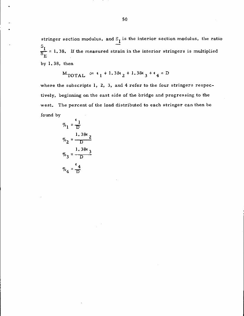
50

stringer section modulus, and s1

is the interior section modulus, the ratio

s I 'S':- = 1. 38. If the measured strain in the interior stringers is multiplied E

by 1. 38, then

M TOT AL o= e 1 + 1. 3 8e 2 + 1. 3 Se 3 + e 4 = D

where the subscripts 1, 2, 3, and 4 refer to the four stringers respec-

tively, beginning on the east side of the bridge and progressing to the

west. The percent of the load distributed to each stringer can then be

found by E 1

%1=1J

1. 38E Z %2 = D

1. 38E 3 %3 = D

51

RESULTS

The main objective of this work was to determine the correlation

between Linger's theoretical impact formula and observed experimental

impact within the upper regions of the theoretical curve. In addition it

was hoped that information relating to the dynamic load distribution could

be obtained.

Due in part to the effects of dynamic load distribution, the test

appears scattered (figures 9 to lZ). Theoretically the stationary oscillator

eliminates the problem of getting the frequencies due to a smoothly rolling

load and due to a repetition of axles in phase at resonance; however,

other difficulties are encountered. The experimental data coincides with

the theoretical data reasonably well in the regions other than at resonance,

and as the theoretical curve approaches resonance the experimental data

becomes farther removed from the theoretical (figure 8). This is true

for frequencies greater than resonance; however, it is not nearly so pro­

nounced for the experimental data at frequencies lower than the resonant

frequency. The shape of the theoretical curve can be changed by changing

the damping factor, and the damping coefficient used in all the theoretical

curves in this work was negl~gible. Possibly a large part of the differ­

ence between theory and test may be accounted for by considering a more

realistic approach to damping. In determining the damping coefficients

for the bridge, an equivalent viscous damping was used. Since structural

damping is proportional to the amount of displacement, it is feasible to

assume that in the region near resonance the damping coefficient would

take on a significant value. The effects of this increased damping would

•

52

be to bend the theoretical curve closer to the observed values, which

are the result of considering the total moment in all four stringers at

the mid-point due to a dynamic load at the center of the bridge (figure 8).

This represents the condition most nearly in accord with the assumptions

made in the derivations of the impact formula. The two most important

assumptions were that the structure under consideration was a simply

supported beam with negligible width as compared to its length, and

that the first term of the Fourier series representing a concentrated

load gives very good approximation to a true concentrated load when both

load and deflection are near the center of the beam.

The test impact as measured in individual stringers can be compared

with the theoretical impact (figures 9 to 12). The results are well

scattered from the theoretical curve, indicating that a closer look at the

derivations might be in order. It would seem that the assumption that

a bridge can be simulated by one beam might cause serious error for

various reasons. In the first place, the nature of a bridge is such that it is

loaded eccentrically. That is, traffic lanes are usually even in number, and·

the loads are applied along lines other than the longitudinal centerline of

the bridge. Though the distribution of static loads to the stringers is

fairly well understood, little is known about the dynamic load distribution

to the stringers. The effects of a dynamic load transferred through a

spring system with damping are not the same as the effects due to an

equal static load applied through the same medium. The slab on a bridge

certainly is analogous to a spring system with internal damping, and

loads applied through this medium can be considered as applied through

53

a spring system with damping. But if the damping is very small the

dynamic effect will be the same as the static effect for all practical

purposes. There may also be a torsional effect which could play a

large part in the dynamic load distribution. With an eccentric dynamic

load on the bridge, a torsional vibration could be set up. This torsional

effect would be greater or less, depending on how close the impressed

frequency was to the natural frequency in torsion.·

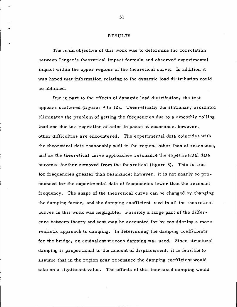
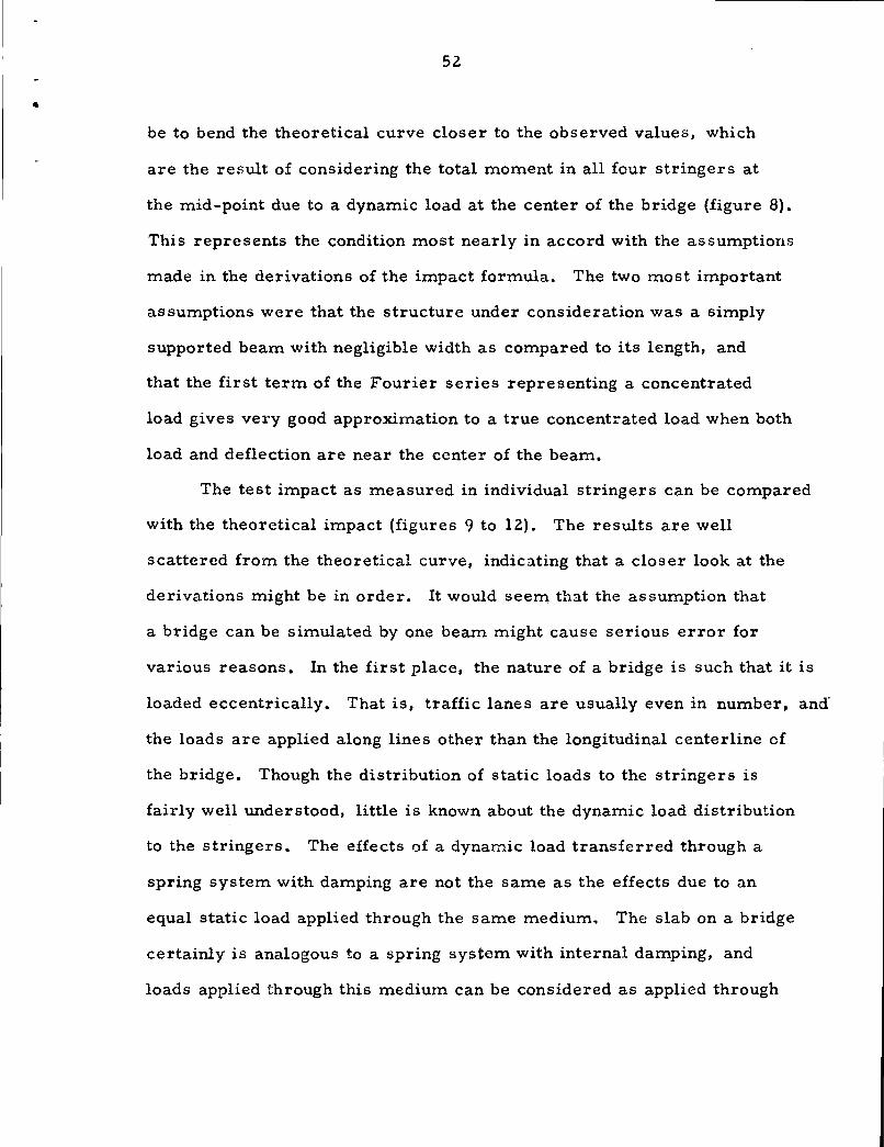
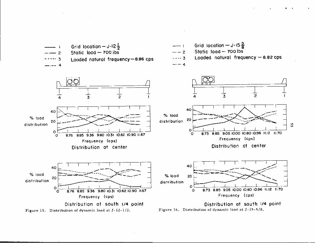
The effects of dynamic loading, shown in figures 13 to 22, repre-

sent the percent of the total moment taken by each of the four stringers

at the center and south quarter point of the bridge respectively due to

oscillating loads applied at those points. The torsional effects should

be most predominant on the series of tests run with the oscillator pur-

posely located in an eccentric position. The distributive nature of the

results, indicate that the effect is directly opposite to what would be

expected from torsion (figures 13 to 17). Up to a point, as the frequency

increases, the percent of the load distributed to the stringers 3 and 4

decreases, and the percent of the load distributed to stringers 1 and 2

increases. If the bridge were vibrating torsionally in phase with the

impressed oscillating load as well as laterally, stringers 3 and 4 would take increasingly larger percentages of load; and strin.gers 1 and 2 should take increasingly smaller pe:rcentages of load. It might be pointed out

that at higher frequencies ther~ is very little pattern to the load distribu-

tion among the stringers. Many of the patterns that have been set up

break down around 10 cycles per second, which is in the region just above

the unloaded natural frequency of the bridge. A very definite beat appeared

on the strain record within these frequencies. The beat was more pro-

nounced in the stringers on the west and receded in the stringers located

40

% load

distribution 20

40

% load

distribution 20

4

I 2 3 4

Grid location- J-6 114 Static load - 700 lbs Loaded natural frequency-

9.20 cps

I I 3 2

8.83 BB5 9.25 9.90 10.38 10.61 II.II 11.52 Frequency (cps)

Distribution at center

.... / -- 7· ... _____ / ............ /· ·-·......:·--::..-~-- :.-<. __...-...-._. ..... / -- ......... --~_,,,,. . ..,.,.. -

0.__~...._~...._~.__~...._~..__---.__~..__~._____..

0 8.83 8.85 9.26 9.90 10.38 10.61 II.II 11.52

Frequency (cps)

Distribution at south 114 point Figure 13. Distribution of dynamic load at J -6-1 /4.

__ , --2

Grid location - J-9 ~ Static load- 100 lbs

---·--· 3 Loaded natural frequency- 8.91 cps ---4

% load

distribution

% load

distribution

4

40

20

I I 3 2

8.61 8.78 9.30 10.31 10.85 11.00 11.62

Frequency (cps)

Distribution at center

40 ·--. ·-·-· ---- ...... -- / -· ---------<"' -...,,,· -------~ ..... ·-~' .... ---·----

20 - - - ·- --. --71"'·· ' . . ' 01____Jl____J~__Jl.......,,---:::-L:---,-:L-,,,........,.-J'-7-::-:-:-'-=-=~'----'

0 9.30 10.31 10.85 11.00 11.62

Frequency (cps)

Distribution at south 114 point

Figure 14. Distribution of dynamic load at J-9-3/8.

I

2

3

-·- 4

4

.. _

40 ',

Grid location - J-12 k Static load - 700 lbs Loaded natural frequency-8.86 cps

I I 3 2

:><·--. ----·-----~,--::,;.-<. % load

distribution

_ ............. 20 --- .

40

% load 20

distribution

8.76 8.85 9.36 9.80 10.31 10.62 10.90 11.67

Frequency (cps)

Distribution at center

--, .. ...... ... .,,,,., ~ .. --·:-::--.:-....,-... ·--·- --~"' - :;.:......-:::: - - -- 7>.'"' _ ...... - - - ~---. .... ............ /-~ -- -- ------·------·

8.76 8.85 9.36 9.80 10.31 10.62 10.90 11.67

Frequency (cps)

Distribution at south 1/4 point Figure 15. Distribution of dynamic load at J-12-1/2.

--1

--2 - - -- 3

-·- 4

40

Grid location - J-15 ~ Static load - 700 lbs Loaded natural frequency - 0.02 cps

I I 4 3 2

% load

distribution 20

% load

distribution

8.73 8.85 9.05 10.00 10.80 10.96 11.12 11.70

Frequency (cps)

Distribution at center

~I I I I I I I l

40 ,./ -- ........ ____ . •.:.::;:.:_:·------.---=-~ -.....2_...·:::------=-·~--- -......... X"'

20 -·~' ......... __

ob-::=~ 0 8.73 8.85 9.05 10.00 10.80 10.96 11.12 11.70

Frequency (cps)

Distribution at south 1/4 point Figure 16. Distribution of dynamic load at J-15-5/8.

V1 V1

56

Grid location - J-1ai - - 2 Static load - 100 I bs ----· 3 Loaded natural frequency- 9.10 cps -·-4

4

40

% load

d istri but ion 20

40

% load 20

d istri but ion

I I 3 2

8.54 8.93 9.35 9.70 10.31 10.78 11.13 11.51 Frequency (cps)

Distribution at center

8.54 8.98 9.35 9.70 10.31 10.78 11.13 11.51

Frequency (cps)

Distribution at south 114 point Figure 17. Distribution of dynamic load at J-18-3/4.

57

more to the east. In other words, stringer 4 usually showed more than

did stringer 1.

Although the load was positioned precisely in the center of the

bridge when loading on the G grid line, the static distribution of moment

in the stringers showed that the force acted a little to the east of center.

Generally speaking, the same "reverse torsional" effects were seen in

the series of tests along the G grid line (figures 18 to 22). That is to

say, those stringers which received the greater share of the load under

static loading, received proportionately less as the frequency increased.

The effect was not so pronounced, but a study of the graphs indicates that

this is true generally.

Although no real conclusions can be drawn from figures 13 through

22., they· are interesting in that they.point out the complex nature of dy­

namic distribution of loads. In this light, then, it seems that the impact

factors previously derived which are based on dynamic reactions in

beams might be found in error due in large part to the nature of dynamic

load distribution when they are experimentally tested on actual highway

bridges.

Figure 23 gives a graphic representation of experimental impact

as related to Linger's formula. There seems to be a fair collaboration

in that the mass of plotted points falls near the theoretical curve; however,

there is still a rather large dispersion. The small range of velocities

is due to the fact that only manpower was available to propel the simu­

lated "truck", and this kept the speed of the vehicle relatively low. A

correlation between this actual truck axle spacing and a fictional axle

spacing applied to the stationary oscillator was not obtained because the

--1

--2 Grid location -G-9 ~ Static load- 100 lbs

3 Loaded natural frequency- 9.07 cps -·- 4

~ IS??I 1 I I .L

4 3 2

40 /·-·-Of I d ~ . . -·-10 oa ---~~::-:::-:.-~-------------- ·-. ~--

0 . ./"' ........ .- __ . ......_-...._ ..............

d . 'b t• 2 "" -1str1 u ion -- -

8.54 8.58 8.92 9.90 10.22 10.80 11.08 11.65

Frequency (cps)

Distribution at center

8.54 8.58 8.92 9.90 10.22 10.80 11.08 11.65

Frequency (cps)

Distribution at south 1/4 point Figure 18. Distribution of dynamic load at G-6-1/4.

I

--1

-- 2

Grid location - G-6 ~ Static load - 100 lbs

3 Loaded natural frequency - 9.15 cps -·- 4

O/o load

distribution

% load

distribution

2 4

40

20

0 0 8.77

40

IR91 l I 3 2

9.09 9.35 9.90 10.73 11.00 11.45

Frequency (cps)

Distribution at center

'---- ................. -------------~<----,. -

20 ·-·--·--· __ .,_,,,,,,,.,. ----.. ........... ' .. , .......... ,' ',,,;,_

8.77 9.09 9.35 9.90 10. 73 11.00 11.45

Frequency (cps)

Distribution at south 1/4 point

Figure 19. Distribution of dynamic load at G-9-3/8.

Q

U1 00

--1

--2 ----- 3

-·-4

40

Grid location - G-12 ~ Static load- 100 lbs Loaded natural frequency- 9.03 cps

~ IS? 91

I I 4 3 2

' .--------·-·-·, % load --- --~------------- .

20 _,;::;..·:~·.- . '- --... A . ---- - ,__. ........ ·' .. --·---·

distribution .......... _____ .....

0:-----:-=-:---:-:----'-----L----L_......i.... _ __L _ _L.._~ 0 8.78 8.87 9.36 9.80 10.32 10. 72 11.20 11.52

Frequency (cps)

Distribution at center

--40 -----:-.---=------- / ---------- -:>-~<.. % load

20 distribution

---·-·-· ......... --- ... ~ .,,. _.,,,,,,,,.·-·---- -" - _, .. -0:---::-=-:----'------'-----1...---1..._......L._.....L _ _L.____J

0 8.78 8.87 9.36 9.80 10.32 10. 72 11.20 11.52 Frequency (cps)

Distribution at south 114 point Figure 20. Distribution of dynamic load at G-12-1/2.

--1

--2 ---- 3

-·- 4

Grid location - G-15f Static load - 100 I bs Loaded natural frequency - 9.06 cps

2 1891 l I I 4 3 2

40

% load

distribution

% load

distribution

20 ::---- .. --·--·-~.:::·-·-· /._.--.,,~c::-- ------. -----

0:-----:"-:-=---l.---l. _ _1. _ __.L__......L._.....L _ _L.._~ 0 8.25 8.92 9.44 9.90 10.32 11.73 11.00 11.62

Frequency (cps)

Distribution at center

o~---:-.:-:---:!--=:::--::1-:--:_i-:-_L_~L_--1~_i____J 0 8.25 8.92 9.44 9.90 10.32 11.73 11.00 11.62

Frequency (cps}

Figure 21. Distribution at south 1/4 point

Distribution of dynamic load at G-15-5/8.

--1

--2 ----· 3

-·-4

I

% load

d . t "b t• 20 IS rl U 100

Grid location-G-18 ~ Static load - 700 lbs Loaded natural frequency- 9.11 cps

IR91 2 I I 4 3 2

2

O'--~'--___J'----'-~---'-~---'-~--'-~--'-~--'-~-' 0 8.60 9.00 9.44 10.00 10.32 10.06 11.00 11.62

40

% load 20

distribution

Frequency (cps)

Distribution at center

8.60 9.00 9.44 10.00 10.32 10.06 11.00 11.62 Frequency (cps)

Distribution at south 114 point Figure 22. Distribution of dynamic load at G-18-3/4.

1.4

1.2

1.0

0.8

Impact

0.6

0.4

0.2

Figure 23.

0

v

' I

5

- Theoretical o Beam I • Beam 2 v Beam 3 ' Beam 4

"Simulated truck" results

10 15 Velocity, ft./sec.

Results of moving load tests.

20

61

oscillator frequencies were too high. Had the oscillator frequency

corresponded to the frequency set on the strobotac, a comparison would

be possible; however, the error in the strobotac frequency prevented

this. The impact was increased as much as three times its normal value

when the truck was pushed over a small obstruction in the bridge. As

would be expected, this impact was greatest when the obstruction was

placed in the center of the bridge. This indicates that conditions which

cannot be completely anticipated in theory or tests must somehow be taken

into account. The truck used in this test was not spring mounted, how­

ever, and this results in a larger impact than if it were spring mounted 1

•

Deviation from the theoretical impact as derived by Linger was

rather large and unpredictable when individual stringers were considered

by themselves, though when considering the bridge as a whole, the corre­

lation was much better. It is interesting to note that the impact which ex­

ceeded the theoretical curve in most occurred in those stringers on the

opposite side of the bridge from where the load was located4

• The

stringers having the greatest impact are those which are able to withstand

the greatest impact, or those which take the least static load.

A more accurate determination of the effects of damping on bridge

structures would provide a much better correlation between theory and test

when considering the bridge as a whole. To consider impact effect on

individual stringers, however, would require a better knowledge of dy-

namic distribution.

62

RECOMMENDATIONS FOR FURTHER STUDY

As is often true in research, more questions are raised than are

answered. This work has not been different in this aspect. Some specific

investigations which could prove beneficial in their results are the following.

( 1) V· hat are the factors affecting dynamic load distribution in

bridge spans, and how are these factors related to the resulting stresses

in bridge members? Because of the very complex nature of this. question,

it seems that the best approach would be to use an empirical method of

attack.

(2) What is the correlation between impact as determined by a sta­

tionary oscillating load and moving vehicle loads on the same bridge?

Tests could be performed on actual highway bridges so that the problem of

moving a vehicle across the bridge, which was present in this study,

would be solved.

(3) V!hat is an effective method for determining the coefficient of

solid damping in bridge structures? If an impact factor is to be based on

bridge vibrations, it would be necessary for a designer in an office to

have a relatively rapid method of designing. or checking a coefficient of

solid damping other than experimenting on the bridge he is designing.

The damping factor will certainly play a large role in determining a

maximum impact, and any knowledge gained in this area would be very

helpful.

63

REFERENCES

1. Biggs, J. M. and Suer, H. S. Vibration measurements of simple­span bridges. Highway Research Board Bulletin 124:1-15. 1955.

2. Bishop, R. E. D. and Johnson, D. C. The mechanics of vibration. The Universary Press, Cambridge. 1960.

3. Caughey, R. A. and Senne, J. H., Distribution of loads in beam and slab bridge floors. Iowa State University of Science and Tech­nology. Final Report, Project 357-S. Iowa Engineering Experiment Station. 1959.

4. Edgerton, R. C. and Beecroft, G. W. Dynamic studies of two con­tinuous plate-girder bridges. Highway Research Board Bulletin 124: 33-46. 1955.

5. Foster, G. M. and Oehler, L. T. Vibration and deflection of rolled­beam and plate-girder bridges. Highway Research Board Bulletin 124:79-110. 1955.

6. Hayes, J. M. and Sbarounis, J. A. Vibration study of three-span continuous I-beam bridge. Highway Research Board Bulletin 124: 4 7 - 78. 19 5 5 •

7. Inglib, C. E. A mathematical treatise on vibration in railway bridges. The University Press, Cambridge. 1934.

8. Linger, D. A. Forced vibration on continuous highway bridges. Ph.D. thesis. Iowa State University Library. 1960.

9. Looney, T. G. High-speed computer applied to bridge impact. Journal of the Structural Division, American Society of Civil Engineers. Vol. 84, Paper 1759. September, 1958.

10. Scheffey, C. F. Dynamic load analysis and design of highway bridges. Highway Research Board Bulletin 124:16-32., 1955.

11. Soroka, W. W. Note on the relations between viscous and structural damping coefficients. Journal of the Aeronautical Sciences. 16:409-410. July, 1949.

12. Standard specifications for highway bridges. The American Associ­ation of State Highway Officials. Washington, D. C. 1957.

13. Stokes, G. G. Discussion of a differential equation relating to the breaking of railway bridges. In Stokes, G. G. Mathematical and physical papers. 2: 179 .. 220. The University Press, Cambridge. 1883.

•

• •'

64

14. Thompson, W. T. Mechanical vibrations. Zd ed. Prentice-Hall, Inc., Englewood Cliffs, N. J. 1959.

15. Timoshenko, S. P. Vibration problems in engineering. 3rd ed. D. Van Nostrand Go., Inc., New York. 1955.

16. Tung, T. P., Goodman, L. E., Chen, T. Y., and Newmark, N. M. Highway-bridge impact problems. Highway Research Board Bulletin 124:111-134. 1955.

17. Vandegriff, L. E. Vibration studies of continuous span bridges. En­gineering Experiment Station Bulletin 119, Ohio State University.

18. Willis, R. Extracts from the appendix of the report of the commis­sioners appointed to inquire into the application of iron to railway structures. In Barlow, P. A treatise on the strength of materials. 6th ed. pp. 326-386. Lockwood and Co., London. 1867.

19. Wise, J. A. Dynamics of highway bridges. Highway Research Board Proceedings 32:180-187. 1953.

•

65

4

ACKNOWLEDGMENTS ' ,

Grateful acknowledgment is made to the Iowa Highway Research

Board who sponsored this project, and to Bob Bacon, whose conscientious

effort and time during the performance of tests and in evaluating data is

gratefully appreciated.