dynamics of matter waves undergoing bloch oscillations in
TRANSCRIPT

UNIVERSIDADE DE SÃO PAULOINSTITUTO DE FÍSICA DE SÃO CARLOS
Lucas Garcia Borges
Dynamics of matter waves undergoing Bloch oscillationsin a ring cavity
São Carlos
2021


Lucas Garcia Borges
Dynamics of matter waves undergoing Bloch oscillationsin a ring cavity
Dissertation presented to the Graduate Pro-gram in Physics at the Instituto de Física deSão Carlos da Universidade de São Paulo, toobtain the degree of Master in Science.
Concentration area: Theoretical and Experi-mental Physics
Advisor: Prof. Dr. Romain Pierre MarcelBachelard
Corrected version(Original version available on the Program Unit)
São Carlos2021

I AUTHORIZE THE REPRODUCTION AND DISSEMINATION OF TOTAL ORPARTIAL COPIES OF THIS DOCUMENT, BY CONVENTIONAL OR ELECTRONICMEDIA FOR STUDY OR RESEARCH PURPOSE, SINCE IT IS REFERENCED.
Borges, Lucas Dynamics of matter waves undergoing Bloch oscillationsin a ring cavity / Lucas Borges; advisor Romain Bachelard- corrected version -- São Carlos 2021. 68 p.
Dissertation (Master's degree - Graduate Program inTheoretical and Experimental Physics) -- Instituto deFísica de São Carlos, Universidade de São Paulo - Brasil ,2021.
1. Bloch oscillations. 2. CARL. 3. EIT. 4. Three-levelatoms. I. Bachelard, Romain, advisor. II. Title.

Primeiramente agradeço aos meus pais, Girceley e Carlos H., e a minha irmã, MariaRita, pelo apoio incondicional em todos os momentos da minha trajetória acadêmica,
apesar de não entenderem bem o que faço. Espero ser sempre capaz de retribuir esse apoio.Este trabalho todo é dedicado a eles.
Quero dedicar também esta monografia ao meu orientador, prof. Romain Bachelard, cujadedicação e colaboração tornaram possível a construção deste trabalho. Tenho muita sortede ter tido a oportunidade de trabalhar e aprender com ele, e ainda mais de conhecê-lomelhor pessoalmente. Agradeço também a todos os professores que me lecionaram durante
esses 6 anos, em especial aos professores Philippe Courteille e Raul Celistrino, cujoempenho e dedicação mantém um exímio grupo de pesquisa, e ao professor Raphael
Santarelli, meu primeiro orientador durante minha graduação.Meu mestrado também não seria possível sem o apoio de todos os amigos que fiz ao longodesta jornada. Agradeço especialmente aos meus amigos de laboratório: Dalila Rivero,Marcia Frometa e Pablo Dias, cujas presenças foram essênciais para tornar essa minhajornada ao longo do mestrado inesquecível, e por acolherem um teórico no meio de tantosexperimentais. Também não posso me esquecer dos amigos que estiveram comigo desde ocomeço da minha graduação, em especial: Aline Chan, que sempre me acolheu e me serviu
a melhor comida de SanCa, te agradeço pessoalmente quando for me visitar; LucasOliveira, cuja presença sempre anima nossos grupos e nunca se esquece de uma dataespecial, obrigado por ser o melhor rommmate que tive; Vinicius Rossi, que apesar desempre estarmos longe e minha constante demanda de atenção, isso nunca abalou nossa
relação.E a todas as outras pessoas que tive a sorte de encontrar ao longo desse caminho, muitoobrigado por todos esses momentos, tristes ou felizes, que tivemos e ainda teremos!


ACKNOWLEDGEMENTS
I wish to thank the Instituto de Física de São Carlos for the support.
I would like to express my great gratitude to Prof. Romain Bachelard for hissupervision and fellowship. And Prof. Philippe Courteille for welcoming me into his group.
This study was financed in part by the Coordenação de Aperfeiçoamento de Pessoalde Nível Superior – Brasil (CAPES) – Finance Code 001.


“It is good to have an end to journey toward;but it is the journey that matters, in the end.”
— Ursula K. Le Guin


ABSTRACT
BORGES, L. Dynamics of matter waves undergoing Bloch oscillations in aring cavity. 2021. 68p. Dissertation (Master in Science) - Instituto de Física de SãoCarlos, Universidade de São Paulo, São Carlos, 2021.
The work developed in this thesis investigate the dynamics of ultracold atoms trapped ina ring cavity and undergoing Bloch oscillations due to the influence of a one-dimensionalvertical optical lattice and of the gravitational force. In this configuration, the atomscollectively scatter light from the pump into the copropagating cavity mode, which thenleads to a self-consistent grating of the matter: this mechanism was coined collective atomicrecoil lasing (CARL). Such interaction between atomic motion and cavity modes provides apossible continuous and non-destructive method to monitor the Bloch oscillations dynamics,which could be implemented in atomic gravimeters. This dissertation investigates thefundamental problem of dissipation effects due to spontaneous emission of the atoms,which is responsible for a suppression of the Bloch oscillations signatures on the lightmodes. We also study a possible solution for this issue by including a third atomic level inthe configuration to explore a probable dissipation reduction due to the phenomenon ofelectromagnetically induced transparency (EIT).
Keywords: Bloch oscillations. CARL. EIT. Gravimetry. Three-level atom.


RESUMO
BORGES, L. Dinâmica de ondas de matéria realizando oscilações de Bloch emuma cavidade anelar. 2021. 68p. Dissertação (Mestre em Ciências) - Instituto de Físicade São Carlos, Universidade de São Paulo, São Carlos, 2021.
O trabalho desenvolvido nesta tese investiga a dinâmica de átomos ultra-frios aprisionadosem uma cavidade anular e submetidos a oscilações de Bloch devido à influência de umarede ótica vertical unidimensional e da força gravitacional. Nesta configuração, os átomosdispersam coletivamente a luz de pump para o modo copropagante da cavidade, o queentão leva a uma organização autoconsistente da matéria: este mecanismo foi cunhado derecoil lasing atômico coletivo (CARL). Tal interação entre os modos de movimento atômicoe cavidade proporciona um possível método contínuo e não destrutivo para monitorar adinâmica das oscilações de Bloch, que poderia ser implementado em gravimetria atômica.Esta dissertação investiga o problema fundamental dos efeitos de dissipação devido àemissão espontânea dos átomos, que é responsável pela supressão das assinaturas dasoscilações de Bloch nos modos de luz. Também estudamos uma possível solução para estaquestão, incluindo um terceiro nível atômico na configuração para explorar uma provávelredução da dissipação devido ao fenômeno da transparência induzida eletromagneticamente(EIT).
Palavras-chave: Oscilações de Bloch. CARL. EIT. Gravimetria. Átomos de três níveis.


LIST OF FIGURES
Figure 1 – Time-dependent quasimomentum q(t) in the first Brillouin zone π/d ≤q ≤ π/d. . . . . . . . . . . . . . . . . . . . . . . . . . . . . . . . . . . . 21
Figure 2 – Time-of-flight images of the atoms recorded for different times of evo-lution in the optical lattice potential. In the upper part of each frame,the atoms confined in the optical lattice perform Bloch oscillations forthe combined effect of the periodic and gravitational potential. In thelower part, untrapped atoms fall down freely under the effect of gravity. 22
Figure 3 – The atom on the left is initially placed on the slope of the stationarywave. When accelerated towards the bottom of the potential, it pushesthe wave to the right, so that the atom initially positioned in the valleyof the potential is then granted potential energy and begins to oscillate. 23
Figure 4 – Scheme of a ring cavity consisting of two high-reflecting mirrors (HR)and one output coupler (OC) interacting with an ultra-cold atoms cloudstored in one arm of the ring cavity. The cavity modes are the pumpand probe modes (α+ and α− respectively). Two lasers (K) crossingthe cavity mode at the location of the cloud under angles β/2 generatean optical lattice whose periodicity is commensurate with the standingwave created by the pump and probe modes. The atoms are also subjectto an external accelerating force mog. . . . . . . . . . . . . . . . . . . . 24
Figure 5 – Diagram of a atom (atomic cloud) excited by two counterpropagatinglight modes in a ring cavity. . . . . . . . . . . . . . . . . . . . . . . . . 31
Figure 6 – Two-level energy diagram for an atom excited by a laser field Ω21, where∆21 is the detuning between the optical field frequency ω and the atomiclevels transition, and Γ21 is the decay rate for the spontaneous emissionof the excited level. . . . . . . . . . . . . . . . . . . . . . . . . . . . . . 33
Figure 7 – Rabi oscillations for the populations difference (ρ11−ρ22)/2 of a two-levelatom with different values for the detuning where λ =
√Ω2 + ∆2. . . . 34
Figure 8 – Rabi oscillations of a two-level atom with spontaneous emission in theresonance regime (∆21 = 0). For increasing decay rate the populationdifference reaches a stationary value faster. . . . . . . . . . . . . . . . . 35
Figure 9 – Typical behaviour for the dipolar and radiative pressure forces in thetwo-level atom system as function of the detuning ∆12 for a decay rate|Ω21| = Γ21/2 = 106Hz, atomic position kz = π/4 and |α+| = 2|α−| =100 . . . . . . . . . . . . . . . . . . . . . . . . . . . . . . . . . . . . . . 37
Figure 10 – Typical level configurations of a three-level atom, where each arrowrepresents a permitted level transition. . . . . . . . . . . . . . . . . . . 39

Figure 11 – Schematic representation of the atomic level system with the transitions(blue and green arrows) excited by the light fields (Ω21 and Ω32) andthe spontaneous decay transitions (red arrows) with respective decayrates (Γ). . . . . . . . . . . . . . . . . . . . . . . . . . . . . . . . . . . 40
Figure 12 – Schematic representation of the Cascade three-level level system withthe transitions (blue and green arrows) excited by the light fields Ω21 andΩ32, and the spontaneous decay transitions (red arrows) with respectivedecay rates Γ21,Γ32,Γ31, where the last one can be neglected in oursystem. . . . . . . . . . . . . . . . . . . . . . . . . . . . . . . . . . . . 43
Figure 13 – Real and imaginary parts of the 3LA coherence σ12 as a function of thedetuning of the transition |1〉 → |2〉 for different pumping strengths Ω32
of transition |2〉 → |3〉. Parameters for the figure are Γ32 = 0.1Γ21 andΩ21 = Γ21. . . . . . . . . . . . . . . . . . . . . . . . . . . . . . . . . . . 45
Figure 14 – Real and imaginary parts of the 3LA coherence σ12 as a function of thedetuning of the transition |1〉 → |2〉 for different pumping strengths Ω32
of transition |2〉 → |3〉. Parameters for the figure are Γ32 = 10Γ21 andΩ21 = Γ21. . . . . . . . . . . . . . . . . . . . . . . . . . . . . . . . . . . 46
Figure 15 – Real and imaginary parts of the coherence σ12 as a function of thedetuning for the complete steady state Bloch equations and excited levelspopulations. Parameters for the figure are Γ32 = Γ21 and Ω21 = 10Γ21.In the right picture, for Ω32/Ω12 = 0, ρ33 = 0 (i.e., the dash-dottedblue curve overlaps with the x-axis) . . . . . . . . . . . . . . . . . . . . 46
Figure 16 – Real and imaginary parts of the coherence σ12 as a function of thedetuning for the complete steady state Bloch equations and excitedlevels populations. Parameters for the figure are Γ32 = 0.1Γ21 andΩ21 = 10Γ21. . . . . . . . . . . . . . . . . . . . . . . . . . . . . . . . . . 47
Figure 17 – Ratio between real and imaginary parts of the transition |1〉-|2〉 coher-ence, varying the values of the decay rate for the transition |2〉-|3〉. Herewe have used Ω32 = 5Ω21 and Ω21 = 5Γ21. The black dashed line is thesolution for Ω23 = 0. . . . . . . . . . . . . . . . . . . . . . . . . . . . . 48
Figure 18 – New resonant peaks in the optical forces steady state solutions, asfunctions of the transition |1〉-|2〉 detuning for different transition |2〉-|3〉 Rabi frequencies. Parameters for the figure are Γ32 = 0.1Γ21 andΩ12 = 10Γ21. . . . . . . . . . . . . . . . . . . . . . . . . . . . . . . . . . 48
Figure 19 – Optical forces in hk as function of transition |1〉-|2〉 detuning and pumpstrength of transition |2〉-|3〉. Parameters for the figures are Γ32 = 0.5Γ21
and Ω12 = 10Γ21. . . . . . . . . . . . . . . . . . . . . . . . . . . . . . . 49
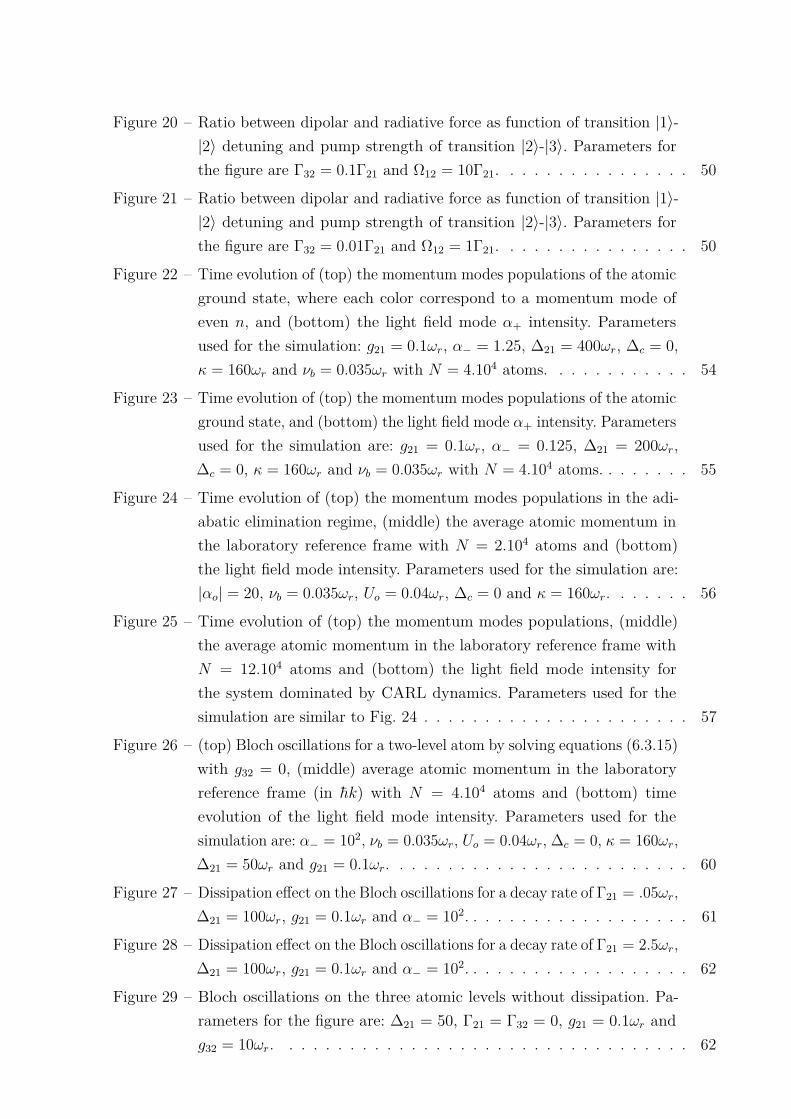
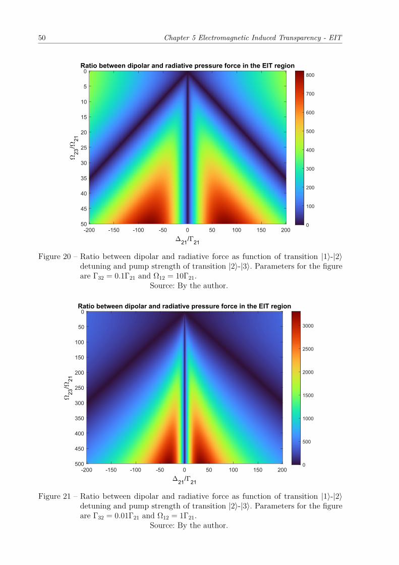
Figure 20 – Ratio between dipolar and radiative force as function of transition |1〉-|2〉 detuning and pump strength of transition |2〉-|3〉. Parameters forthe figure are Γ32 = 0.1Γ21 and Ω12 = 10Γ21. . . . . . . . . . . . . . . . 50
Figure 21 – Ratio between dipolar and radiative force as function of transition |1〉-|2〉 detuning and pump strength of transition |2〉-|3〉. Parameters forthe figure are Γ32 = 0.01Γ21 and Ω12 = 1Γ21. . . . . . . . . . . . . . . . 50
Figure 22 – Time evolution of (top) the momentum modes populations of the atomicground state, where each color correspond to a momentum mode ofeven n, and (bottom) the light field mode α+ intensity. Parametersused for the simulation: g21 = 0.1ωr, α− = 1.25, ∆21 = 400ωr, ∆c = 0,κ = 160ωr and νb = 0.035ωr with N = 4.104 atoms. . . . . . . . . . . . 54
Figure 23 – Time evolution of (top) the momentum modes populations of the atomicground state, and (bottom) the light field mode α+ intensity. Parametersused for the simulation are: g21 = 0.1ωr, α− = 0.125, ∆21 = 200ωr,∆c = 0, κ = 160ωr and νb = 0.035ωr with N = 4.104 atoms. . . . . . . . 55
Figure 24 – Time evolution of (top) the momentum modes populations in the adi-abatic elimination regime, (middle) the average atomic momentum inthe laboratory reference frame with N = 2.104 atoms and (bottom)the light field mode intensity. Parameters used for the simulation are:|αo| = 20, νb = 0.035ωr, Uo = 0.04ωr, ∆c = 0 and κ = 160ωr. . . . . . . 56
Figure 25 – Time evolution of (top) the momentum modes populations, (middle)the average atomic momentum in the laboratory reference frame withN = 12.104 atoms and (bottom) the light field mode intensity forthe system dominated by CARL dynamics. Parameters used for thesimulation are similar to Fig. 24 . . . . . . . . . . . . . . . . . . . . . . 57
Figure 26 – (top) Bloch oscillations for a two-level atom by solving equations (6.3.15)with g32 = 0, (middle) average atomic momentum in the laboratoryreference frame (in hk) with N = 4.104 atoms and (bottom) timeevolution of the light field mode intensity. Parameters used for thesimulation are: α− = 102, νb = 0.035ωr, Uo = 0.04ωr, ∆c = 0, κ = 160ωr,∆21 = 50ωr and g21 = 0.1ωr. . . . . . . . . . . . . . . . . . . . . . . . . 60
Figure 27 – Dissipation effect on the Bloch oscillations for a decay rate of Γ21 = .05ωr,∆21 = 100ωr, g21 = 0.1ωr and α− = 102. . . . . . . . . . . . . . . . . . . 61
Figure 28 – Dissipation effect on the Bloch oscillations for a decay rate of Γ21 = 2.5ωr,∆21 = 100ωr, g21 = 0.1ωr and α− = 102. . . . . . . . . . . . . . . . . . . 62
Figure 29 – Bloch oscillations on the three atomic levels without dissipation. Pa-rameters for the figure are: ∆21 = 50, Γ21 = Γ32 = 0, g21 = 0.1ωr andg32 = 10ωr. . . . . . . . . . . . . . . . . . . . . . . . . . . . . . . . . . 62

Figure 30 – Bloch oscillations on two atomic levels with dissipation. Parametersfor the figure are: ∆21 = 50, Γ21 = 0.05ωr, Γ32 = 0, g21 = 0.1ωr andg32 = 0ωr. . . . . . . . . . . . . . . . . . . . . . . . . . . . . . . . . . . 63
Figure 31 – Bloch oscillations on three atomic levels with dissipation. Parametersfor the figure are: ∆21 = 50, Γ21 = 0.05ωr, Γ32 = 0, g21 = 0.1ωr andg32 = 10ωr. . . . . . . . . . . . . . . . . . . . . . . . . . . . . . . . . . 63

CONTENTS
1 INTRODUCTION . . . . . . . . . . . . . . . . . . . . . . . . . . . . 191.1 Bloch Oscillations . . . . . . . . . . . . . . . . . . . . . . . . . . . . . 201.2 Collective Atomic Recoil Lasing . . . . . . . . . . . . . . . . . . . . . 221.3 Proposed set-up . . . . . . . . . . . . . . . . . . . . . . . . . . . . . . 23
2 MANY-ATOM OPTICAL BLOCH EQUATIONS . . . . . . . . . . . 252.1 Density matrix . . . . . . . . . . . . . . . . . . . . . . . . . . . . . . . 252.2 Dipole approximation . . . . . . . . . . . . . . . . . . . . . . . . . . . 272.3 Rotating wave approximation . . . . . . . . . . . . . . . . . . . . . . . 282.4 Master equation . . . . . . . . . . . . . . . . . . . . . . . . . . . . . . 29
3 TWO-LEVEL ATOMS . . . . . . . . . . . . . . . . . . . . . . . . . . 313.1 Bloch equations for two-level systems . . . . . . . . . . . . . . . . . . 313.2 Matrix representation . . . . . . . . . . . . . . . . . . . . . . . . . . . 323.3 Reduced Bloch equations . . . . . . . . . . . . . . . . . . . . . . . . . 333.4 Stationary case . . . . . . . . . . . . . . . . . . . . . . . . . . . . . . . 343.5 Optical fields . . . . . . . . . . . . . . . . . . . . . . . . . . . . . . . . 353.6 Optical forces . . . . . . . . . . . . . . . . . . . . . . . . . . . . . . . . 36
4 THREE-LEVEL ATOM . . . . . . . . . . . . . . . . . . . . . . . . . 394.1 Bloch equations for three-level system . . . . . . . . . . . . . . . . . 394.2 Stationary case . . . . . . . . . . . . . . . . . . . . . . . . . . . . . . . 414.3 Optical Fields . . . . . . . . . . . . . . . . . . . . . . . . . . . . . . . . 424.4 Optical Forces . . . . . . . . . . . . . . . . . . . . . . . . . . . . . . . . 42
5 ELECTROMAGNETIC INDUCED TRANSPARENCY - EIT . . . . 435.1 Static description of EIT . . . . . . . . . . . . . . . . . . . . . . . . . 435.2 EIT in presence of spontaneous emission . . . . . . . . . . . . . . . . 445.3 Radiative pressure force reduction . . . . . . . . . . . . . . . . . . . . 47
6 MATTER-WAVES AND REPRESENTATION INMOMENTUM SPACE 516.1 Quantum momentum operator . . . . . . . . . . . . . . . . . . . . . . 516.2 Schrödinger equation for the two-level atoms . . . . . . . . . . . . . 536.3 Master equation for the three-level atoms . . . . . . . . . . . . . . . 566.4 Results . . . . . . . . . . . . . . . . . . . . . . . . . . . . . . . . . . . . 60
7 CONCLUSIONS . . . . . . . . . . . . . . . . . . . . . . . . . . . . . 65

REFERENCES . . . . . . . . . . . . . . . . . . . . . . . . . . . . . . 67
19
1 INTRODUCTION
The measurement of the gravitational field is an important objective in the fieldsof geophysics, metrology, and many others as it provides informations of the planet’smorphology and on the composition of the underground. In particular, a precise measureof the local gravity acceleration can have a strong impact on oil exploration, considering itcould completely replace invasive methods, which are very costly. Since the last century,gravimetry has evolved from pendulums, springs, torsion balances and superconductinglevitation instruments1 until recently, to cold atom interferometry.2 The latter takesadvantage of an oscillatory phenomenon known as the atomic Bloch oscillations.
The phenomenon of Bloch oscillations was predicted theoretically by Felix Bloch in19293 in a study of electrons in a periodic crystal potential, where it had been demonstratedthat the application of a constant force on the confined electrons produces an oscillatorybehavior instead of a uniform movement. Back in the 90’s, the same phenomenon wasdemonstrated in cold atoms trapped in optical lattices when an external force was applied,4
thus the name atomic Bloch oscillations.
The oscillations of the matter-waves due to the conservative potential provide adirect signature of the force, hence the potential for gravimetry. This was recently shownby the first measurements of gravity by that means,2,5–7 reaching precisions of 10−7. Thismakes Bloch oscillations a useful tool with a wide range of applications, e.g., oil prospectionand metrology. However, experiments up to date have the disadvantage of relying ondestructive measurements of the instantaneous velocity of the atoms, such as absorptionimaging, which shatters the atomic cloud so a new ensemble is required to continue theoscillations measure. Consequently, thousands of realizations must be performed in orderto produce a precise measurement of the force field, which in turn is spoiled by fluctuationsin the cloud preparation, and requires more time for the integration.
To tackle the problem of destructive measurements, one possible solution is tocombine the collective atomic effect of CARL (collective atomic recoil lasing), together withthe Bloch oscillations, using the particularities of a ring cavity, as proposed by the projectcollaborators.8–10 As the counterpropagating modes of the ring cavity have independentphoton numbers, it allows a continuous harness of the light pulses resulting from the Blochoscillations. This continuous measurement depends on a single realization, eliminatingproblems of fluctuations between realizations and drastically reducing the integrationtime. Consequently, the construction of an experiment to provide the first non-destructivemeasurement of Bloch oscillations by cold atoms was initiated in São Carlos, Brazil, withthe support of the São Paulo Research Foundation (FAPESP), the Brazilian NationalCouncil for Scientific and Technological Development (CNPq) and the Coordination for

20 Chapter 1 Introduction
the Improvement of Higher Education Personnel (CAPES).
This project aims to continue the theoretical investigations of the continuousmonitoring of Bloch oscillations in vertical ring cavities. Although a proof of principle hasrecently been proposed,8 there are still caveats regarding dissipative effects, whose effecton the synchronization of oscillations has not been studied. The research of this thesisarises from the idea of including an additional atomic level in the used model of a two-levelatom, to make use of the EIT (electromagnetic induced transparency) effect: this allowsone to tune the optical characteristics of the atomic ensemble and reduce dissipative forcesthat arise from the light-matter interaction.
In the following sections, we present a brief review of the Bloch oscillations andCARL phenomena.
1.1 Bloch Oscillations
As mentioned earlier, Bloch oscillations were predicted since the first half of lastcentury, but their observation in electrons is very challenging, mostly because of thescattering events by the lattice defects or impurities in natural crystals. On the other hand,in optical systems the relative absence of defects in optical lattice provides an excellentplatform to observe such phenomenon.
To observe the Bloch oscillations with an atomic matter wave, we can considertwo counterpropagating laser fields modes of equal intensity, with wave-number k, whichproduce a one-dimensional stationary wave (the optical lattice). The dynamics occurs inthe presence of an homogeneous and constant force, which in our case is the gravitationalforce. We can write the Schroedinger equation to describe the time evolution of a singleatom wave-function in the presence of the force and of an optical lattice:
ih∂
∂tψ(x, t) = (H− Vg(x))ψ(x, t), (1.1.1)
where we have defined the gravitational potential Vg = mgx, and the one-dimensionalHamiltonian H composed of the atom kinetic energy and the optical lattice potential:
H = p2
2m + Vo cos2(kz), (1.1.2)
with the atomic mass m, the gravitational acceleration g and Vo the optical lattice strength.From the Bloch oscillations theory11,12 we define the eigenfunctions ϕn,q(x) of H as
ϕn,q(x) = eiqxUn,q(x), (1.1.3)
which depends on the position x, the band index n and the quasimomentum q, restrictedto the first Brillouin zone: −k ≤ q ≤ k. The periodic function Un,q(x) = Un,q(x+ π/k) hasthe same periodicity as the optical lattice and satisfy the Schroedinger equation[
(p+ hq)2
2m + Vo cos2(kz)]Un,q(x) = εn,qUn,q(x), (1.1.4)
1.1 Bloch Oscillations 21
where εn,q are the eigenvalues of H, and periodic functions of the quasimomentum q withperiod 2k. The action of the external force F = mg on the system dynamics is incorporatedin the wavefunction by performing a transformation of ψ to the accelerated frame:
ψ(x, t) = eiFxt/hψ(x, t), (1.1.5)
then, equation (1.1.1) becomes
ih∂
∂tψ(x, t) =
[(p+ Ft)2
2m + Vo cos2(kz)]ψ(x, t). (1.1.6)
Comparing equation (1.1.6) to (1.1.4), we observe that the quasimomentum evolves in thepresence of the applied external force F according to
q(t) = q(0) + Ft
h. (1.1.7)
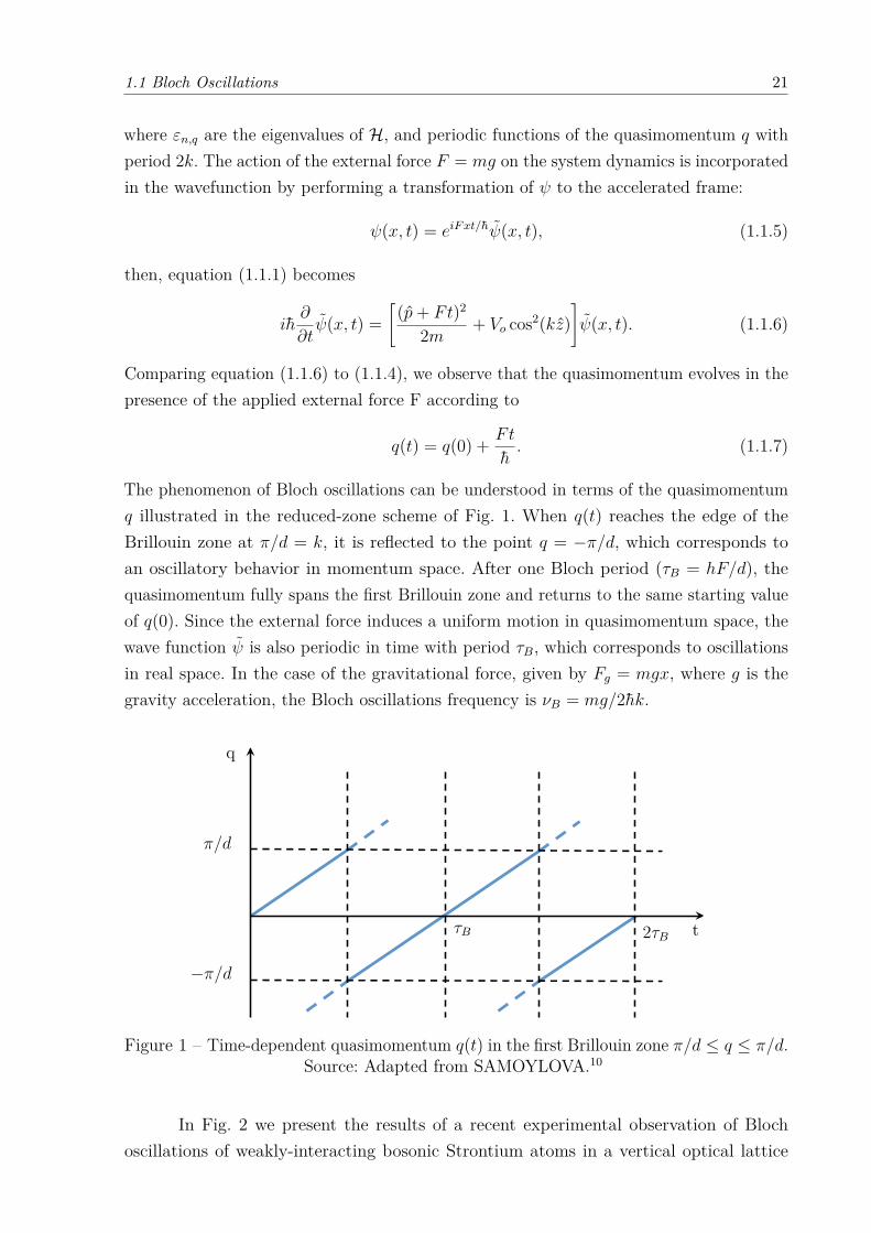
The phenomenon of Bloch oscillations can be understood in terms of the quasimomentumq illustrated in the reduced-zone scheme of Fig. 1. When q(t) reaches the edge of theBrillouin zone at π/d = k, it is reflected to the point q = −π/d, which corresponds toan oscillatory behavior in momentum space. After one Bloch period (τB = hF/d), thequasimomentum fully spans the first Brillouin zone and returns to the same starting valueof q(0). Since the external force induces a uniform motion in quasimomentum space, thewave function ψ is also periodic in time with period τB, which corresponds to oscillationsin real space. In the case of the gravitational force, given by Fg = mgx, where g is thegravity acceleration, the Bloch oscillations frequency is νB = mg/2hk.
t
q
π/d
−π/d
τB 2τB
Figure 1 – Time-dependent quasimomentum q(t) in the first Brillouin zone π/d ≤ q ≤ π/d.Source: Adapted from SAMOYLOVA.10
In Fig. 2 we present the results of a recent experimental observation of Blochoscillations of weakly-interacting bosonic Strontium atoms in a vertical optical lattice

22 Chapter 1 Introduction
under the action of the gravitational potential.5 Each image shows a different realization ofthe experiment, since the time-of-flight method to measure the atoms momentum destroysthe cloud, and a new ensemble had to be prepared to continue the experiment.
3.2 ms2.4 ms 4.0 ms 4.8 ms
Figure 2 – Time-of-flight images of the atoms recorded for different times of evolutionin the optical lattice potential. In the upper part of each frame, the atomsconfined in the optical lattice perform Bloch oscillations for the combined effectof the periodic and gravitational potential. In the lower part, untrapped atomsfall down freely under the effect of gravity.
Source: Adapted from FERRARI.5
1.2 Collective Atomic Recoil Lasing
The collective atomic recoil laser (CARL) consists of the coherent amplificationof the scattered light from an atomic cloud interacting with a counterpropagating laserbeam. It was first predicted13 as an atomic analogue of the free-electron laser (FEL), sinceit converts atomic momentum into coherent radiation.
The concept involves a monochromatic homogeneous beam of two-level atomsmoving at the same velocity and a strong counterpropagating pump laser beam, whichis Bragg-scattered by the atomic density defects. The interference between pump andscattered light then produces an optical potential, which in turns increases the densitygrating in a self-amplifying mechanism. Therefore, the CARL converts kinetic energy intocoherent radiation, increasing the energy difference between probe and pump mediated byatomic bunching. The collective action of the atoms is depicted in Fig. 3.
The feedback of a single atom on the phase of the standing light wave is very weak,thus it is necessary to have many atoms moving collectively, and the phase of the standingwave needs to be not fixed. To satisfy these conditions, a ring cavity can be used, sincethe phase of the standing wave is not fixed by boundary conditions of the mirror surfaces;this is the motive why the first experimental realization of CARL used a ring cavity.15
Furthermore, the counterpropagating fields in a ring cavity form separate modes carryingindependent numbers of photons, which allows to measure independently their photonpopulation. In addition the atoms self-arrange as they are trapped by the dipolar forces inthe antinodes of the stationary wave, which then allows for the observation of the atomicmovement backaction using the phase of the standing wave.
Considering that the pump mode intensity |αp|2 is constant into the cavity, we aimat monitoring the evolution of the probe mode α, where |αp|2 is the photon number. Thecoupling between the modes only happens in the presence of atoms due to backscattering

1.3 Proposed set-up 23
Pump
Time
Probe
Figure 3 – The atom on the left is initially placed on the slope of the stationary wave.When accelerated towards the bottom of the potential, it pushes the wave tothe right, so that the atom initially positioned in the valley of the potential isthen granted potential energy and begins to oscillate.
Source: Adapted from COURTEILLE.14
events and is given by the single-photon light shift Uo = Ωp/∆, given by the rate betweenthe single-photon Rabi frequency and the detuning from the atomic resonance, respectively.We can write the mode rate equation for α as15
α = −κα + iNUoαp∑j
e2ikxj , (1.2.1)
where κ is the cavity decay, which describes the photon loss through the cavity mirror, kis the light modes wavenumber, xj is the j-th atom position and N the number of atoms.The second term in the above expression is the photon gain of the probe from the pumpmode through backscattering. The atom at position xj feels the classical potential of thestationary light wave as the dipolar force, then the dynamics of the atom through thescattering process is given by this force in the far detuned regime15
mxj = −2ihkUo(αpα∗eikxj − α∗pαe−ikxj ). (1.2.2)
1.3 Proposed set-up
The setup investigated in this thesis consists of a cloud of ultracold atoms confinedin a vertical optical standing wave, as depicted in Fig. 4, where it is possible to combineboth effects of Bloch oscillations and the CARL. The optical lattice, with the latticeconstant π/kl, is generated by two external laser beams detuned sufficiently far from theatomic resonance and intersecting at the location of the atoms under the angle β definedby K sin(β/2) = kl, where K is the wavenumber of the laser beams.10 This externallyimposed optical lattice traps the atoms in a one-dimensional potential hWo sin(2kz) alongthe z axis, where the potential depth is denoted by hWo. In addition, the atoms are alsoexposed to the gravitational potential mogz, where mo is the atomic mass and g is the

24 Chapter 1 Introduction
gravitational acceleration. As a result, the atoms undergo Bloch oscillations with frequencyνb = mg/2hk4 under the influence of the applied gravitational force.
α+
α− Latticebea
ms
zg
HR
HR
OC
K
β
k
Figure 4 – Scheme of a ring cavity consisting of two high-reflecting mirrors (HR) and oneoutput coupler (OC) interacting with an ultra-cold atoms cloud stored in onearm of the ring cavity. The cavity modes are the pump and probe modes (α+and α− respectively). Two lasers (K) crossing the cavity mode at the locationof the cloud under angles β/2 generate an optical lattice whose periodicity iscommensurate with the standing wave created by the pump and probe modes.The atoms are also subject to an external accelerating force mog.
Source: Adapted from SAMOYLOVA.10
In Chapter 2, we derive the Bloch equations for a multi-level atom system, usingthe master equation approach since we are interested in describing the dissipation effects ofspontaneous emission in our system. The general equations are used in following Chapters3 and 4, where they are adapted to the two- and three-level atoms, respectively. We alsoperform an analysis of the stationary solutions, optical forces and the light field dynamicsfor those systems.
We describe the EIT effect using the three-level atom equations in chapter 5. Thenwe show the impact of the third level on the optical forces and the radiative pressure forcereduction that can be generated.
The Bloch oscillations in both two- and three-level atoms are derived in Chapter 6,where we use a momentum expansion for the atomic wave-function. First we reproduceresults for the 2LA adiabatic elimination case, studied in previous works. Then, we derivethe von Neumann equation for the three-level system to observe the dissipations effectsand the third level impact on the Bloch oscillations.

25
2 MANY-ATOM OPTICAL BLOCH EQUATIONS
To obtain the equations that describe the CARL dynamics, we must first derivethe equations for the internal degrees of freedom of the atoms. To solve this problem, wecould use the Schroedinger equation and describe the temporal evolution of the state ofthe system. However, within this formalism, we cannot describe the dissipative process ofspontaneous emission as the atom is led to an overlap of many states of momentum andhas to be described by a distribution of wave functions.
To calculate the probability of finding the system within this distribution, weuse the formalism of the density matrix operators that describes a statistical mixture ofquantum states. The equations that describe the temporal evolution of the elements ofthe density matrix of an atom in a field are the optical Bloch equations16 (not related tothe Bloch oscillations, although named after the same person). The following derivationaims to introduce the notation and terminology used throughout this thesis and establishthe dynamical equations for the next chapters.
2.1 Density matrix
Let us consider some atoms trapped in an optical cavity. We call Ψ the atomicwave-function, whose discrete states of quantized degrees of freedom can be described bythose eigenfunctions ψj of the unperturbed Hamiltonian operator Ho. The Hamiltonianeigenvalues define the set of energy levels Ej given by hωj related by
Ho |ψj〉 = hωj |ψj〉 , (2.1.1)
〈r|ψj〉 = ψj(r), (2.1.2)
where j ∈ N. The eigenstates ψj form a complete orthonormal basis∫ψ∗jψkd~r = δjk, (2.1.3)
with δjk being the Dirac delta function. The atomic wave-function Ψ(r, t) satisfies theSchrödinger equation
ih∂Ψ∂t
= HΨ, (2.1.4)
where H is the system Hamiltonian, composed of the Hamiltonians of the unperturbedatom (Ho), the light field (Hfield) and the interaction between them (Hint):
H = Ho +Hfield +Hint. (2.1.5)

26 Chapter 2 Many-atom optical Bloch equations
The unperturbed, or atomic Hamiltonian can be written as the sum of the kineticenergy and the Nl atomic levels |ψj〉 energies
Ho = − h2
2mo
∇2 +Nl∑j=1
hωj |ψj〉〈ψj| , (2.1.6)
where mo is the atomic mass.
The atoms are driven by a near-resonance monochromatic laser, with frequencyslightly detuned from the atomic resonance, which allows the particles to absorb theincoming photons and transition between energy levels. We consider an electric field due toa monochromatic electromagnetic wave17 which, at the atomic position r, can be writtenas
E(r, t) = 12(E+(r, t) + E−(r, t)
), (2.1.7)
E+(r, t) = E aei(k·r−ωt)e = E−(r, t)†. (2.1.8)
a is the annihilation operator of the field mode, k is the field wave-vector and ω itsfrequency with E = i
(hω
2ε0V
)1/2, where V is the cavity volume. The Hamiltonian for this
light field is given byHfield = hωa†a. (2.1.9)
We can solve equation (2.1.4) by the expansion of Ψ in the orthonormal basis ofthe Nl unperturbed atomic states |ψj〉
|Ψ(r, t)〉 =Nl∑j=1
cj(t) |ψj(r)〉 , (2.1.10)
〈ψj(r)|ψj(r)〉 = δjk, (2.1.11)
where cj are the complex amplitudes. For the free-atom case, where H = Ho, we can seethat its time dependence is given by
cj(t) = cj(0)e−iωjt. (2.1.12)
Considering that the eigenstates in (2.1.2) form a orthonormal basis we can define thedensity matrix ρ
ρ = |Ψ〉〈Ψ| , (2.1.13)
whose elements are given byρ =
∑j,k
c∗jckρjk. (2.1.14)
We have here introduced
ρjk = |ψj〉〈ψk| , (2.1.15)
ρjk = c∗jck, ρ∗jk = ρkj, (2.1.16)
with diagonal elements corresponding to energy levels occupations, populations, andoff-diagonal elements being related to the coherences between different levels.

2.2 Dipole approximation 27
2.2 Dipole approximation
In the presence of the light field the electron cloud of the atom is distorted inthe direction of the electric field, inducing an effective electric dipole in the system. Theinduced dipole oscillates and radiates electromagnetic waves as a classical oscillating dipolewould, therefore modifying the electric field.18 To derive the interaction Hamiltonian forthe Bloch equations we begin by calculating the polarization vector, which is obtainedfrom the sum of the dipole moments of each atom in the system
P =∑i
diδ(r− ri). (2.2.1)
We have here defined the induced-dipole moment operator di of the i-th atom as
di = −er, (2.2.2)⟨di⟩
= −e 〈Ψi| r |Ψi〉 , (2.2.3)
where e is the electron charge. Performing the wave-functions expansion (2.1.10) in theunperturbed states we get
⟨d⟩
= −e∑j,k
ρkjpjk, (2.2.4)
with the definition of the time-independent dipole matrix elements:
pjk = −e 〈ψj| r |ψk〉 , p∗jk = pkj. (2.2.5)
In the presence of the external field the momentum part of the unperturbed Hamiltonianis modified into
h2∇2
2mo
→ 12mo
[−ih∇+ eA(r, t)]2 − eΦ(r, t), (2.2.6)
where A(r, t) and Φ(r, t) are respectively the vector and scalar potentials of the externalfield and p is the momentum operator in the atomic Hamiltonian (2.1.6). In the Coloumbgauge the vector potential satisfies the wave function
∇2A− 1c2∂2A∂t2
= 0, (2.2.7)
with solution A = A0eikr−iωkt − c.c., where k = 2π/λ is the field wave-vector and λ its
wavelength. Considering r comparable with typical atomic dimensions (∼ Å), and opticalwavelengths (400− 700nm), one has kr 1; hence over the extent of an atom the vectorpotential can be considered spatially uniform A(r, t) ' A(t), which is referred as the“dipole approximation”. In this gauge, and after a unitary transformation, equation (2.2.6)becomes
12mo
[−ih∇+ e(A +∇χ)]2 − e∂χ∂t. (2.2.8)

28 Chapter 2 Many-atom optical Bloch equations
Choosing the gauge function χ(r, t) = −A · r, we obtain the following relations
∇χ = −A, (2.2.9)∂χ
∂t= −r · ∂A
∂t= −r · E. (2.2.10)
Considering the Hamiltonian in equation (2.1.5) we can identify the interactionHamiltonian in the above equations as
Hint = −d · E. (2.2.11)
Although the interaction between atom and light in the dipole approximation considersa locally constant electric field, it is valid only over the atom size, and it changes withits position relative to the light field wave. Thus, since our system relies on momentumexchange between matter and light, it is still necessary to consider the spatial variation ofE through e±ikr in equation (2.1.8), which describes the atom momentum recoil due to anphoton absorption/emission.
2.3 Rotating wave approximation
Considering the atomic dipole moment in the direction of the electric field, theatom-field interaction Hamiltonian becomes
Hint = 12
Nl∑j,l
(ρljpjl + ρjlplj)(E+(r)e−iωt + E−(r)eiωt
). (2.3.1)
In the unperturbed case the density matrix elements ρjl evolves according toρjl(t) = ρjl(0)e−iωjlt, where ωjl = ωj − ωl, thus the products ρjlE+e−iωt and ρljE−eiωt
rotate much faster than the optical frequency, for a positive ωjl. Hence we can neglectsuch terms performing the denominated rotating wave approximation (RWA).19 One canalso argue that these terms do not conserve energy (in first-order processes) since they canbe interpreted as the absorption of a photon combined with the de-excitation of the atom,or with the emission of a photon combined with the excitation of the atom, respectively.Anyhow, the interaction Hamiltonian can then be approximated as
HRWAint = h
2
Nl∑j>l
(Ωjlρjl + h.c.), (2.3.2)
with the Rabi frequency defined as
Ωjl = plj · E+(r)h
. (2.3.3)

2.4 Master equation 29
2.4 Master equation
Let us now derive the dynamical equations for the density matrix elements consid-ering the effect of spontaneous emission using the master equation formalism through thevon Neumann equation for ρ:
˙ρ = i
h[ρ,H] + Ldρ. (2.4.1)
H is the total Hamiltonian (2.1.5) after the RWA, and Ldρ is the dissipative term,denominated the Lindblad superoperator20:
Ldρ =∑j,k
γjk(2ρkj ρρjk − ρjkρkj ρ− ρρjkρkj), (2.4.2)
with γjk = Γjk/2 the linewidth of the atomic levels transition of |ψj〉 to |ψk〉.
The density matrix elements derivatives can be derived as
ρjk = i
h〈j| [ρ,H] |k〉+ 〈j| Ldρ |k〉 , (2.4.3)
which leads to the following expression for the coherent part:
i
h〈j| [ρ,H] |k〉 = −iωjkρjk −
i
2
Nl∑l>m
(Ωlmρmkδlj + Ω∗lmρlkδmj − Ωlmρjlδmk − Ω∗lmρjmδlk),
(2.4.4)where ωjk = ωj − ωk. For the dissipative part we have
〈j| Ldρ |k〉 =∑l
2γklδjkρll −∑l
(γlj + γlk)ρjk. (2.4.5)
Gathering the expressions above, we obtain the optical Bloch equations with thespontaneous emission, which describes the time evolution of the density matrix elementsfor a Nl-level atom system:
dρjkdt = 2
Nl∑l
γklρllδjk −
Nl∑l
(γlj + γlk) + iωjk
ρjk+ i
2
Nl∑l>m
(Ωlmρmkδlj + Ω∗lmρlkδmj − Ωlmρjlδmk − Ω∗lmρjmδlk). (2.4.6)


31
3 TWO-LEVEL ATOMS
In this chapter we apply the definitions and equations made so far to the simplecase of two-level atoms (2LA) excited by counterpropagating light fields. In this specificcase we consider the derived Bloch equations in chapter 2 setting Nl = 2.
3.1 Bloch equations for two-level systems
We here consider a single atom with only two accessible energy levels denominated|1〉 and |2〉, respectively the non-degenerate ground and excited state. The electric fieldof the incident light field with two counter-propagating modes is given in the Heisenbergpicture by
E(z, t) = ReE(a+e
ikz + a−e−ikz
)e−iωt
e, (3.1.1)
with
E = i
(hω
2ε0V
)1/2
. (3.1.2)
a± are the annihilation operators of the field modes, which satisfy the commutationrelations
[a†±, a±
]= 1 and [a±, a∓] = 0, k is the wave-vector of the modes and ω their
frequency. The field polarization is set in the same direction e of the atomic dipole.
α+ α−
Figure 5 – Diagram of a atom (atomic cloud) excited by two counterpropagating lightmodes in a ring cavity.
Source: By the author.
With the electric field definition, the Hamiltonian in the rotating wave approxima-tion for the 2LA writes
H = − h2
2mo
∇2 − h∆21 |2〉〈2|+ hωa†±a± + hg21a†±e∓ikz |1〉〈2|+ h.c., (3.1.3)
where g21 = d12E/2h is the light-atom coupling force.

32 Chapter 3 Two-level Atoms
Since there is no dipole element between the same levels (pjj = 0), from (2.2.4)the electric dipole moment for the 2LA reads⟨
d⟩
= −e(ρ12p21 + ρ21p12), (3.1.4)
= d12(ρ12 + ρ21)e, (3.1.5)
where we have introduced the electric dipole moment d12 e = −ep12 = −ep21, given by
d12 =√
3πε0hΓ12
k3 , (3.1.6)
and Ω21 the real Rabi frequency for this two-level system, defined as in equation (2.3.3)
hΩ21 =⟨d · E
⟩, (3.1.7)
Ω21 = d12Eh
(α+eikz + α−e
−ikz). (3.1.8)
With those definitions, and after some algebra, we obtain the Bloch equations forthe 2LA from the general expression in (2.4.6), which are given by the following set ofordinary differential equations
dρ11
dt = 2γ2ρ22 + i
2(Ω∗21ρ21eiωt − Ω21ρ12e
−iωt), (3.1.9a)dρ22
dt = −2γ2ρ22 −i
2(Ω∗21ρ21eiωt − Ω21ρ12e
−iωt), (3.1.9b)dρ12
dt = −(γ12 − iω21)ρ12 −i
2Ω∗21eiωt(ρ11 − ρ22), (3.1.9c)
dρ21
dt = −(γ21 + iω21)ρ21 + i
2Ω21e−iωt(ρ11 − ρ22). (3.1.9d)
Remark that it is necessary to add the term γ21ρ22 to the derivative of the firstlevel population to satisfy the constraint of fixed total population:
ρ11 + ρ22 = 1.
3.2 Matrix representation
Let us now rewrite the Bloch equations into the frame of the driving field, byintroducing the following variables, which correspond to the |1〉-|2〉 transition coherence:
ρ21 = σ21e−iωt. (3.2.1)
Then equation (3.1.9d) becomes
ddt(σ21e
−iωt)
= −(γ21 + iω21)σ21e−iωt + i
2Ω21e−iωt(ρ11 − ρ22), (3.2.2)
dσ21
dt = −(γ21 − i∆21)σ21 + i
2Ω21(ρ11 − ρ22), (3.2.3)

3.3 Reduced Bloch equations 33
where ∆21 = ω − ω21 is the detuning between atomic resonance and the field frequency.Therefore we can write the Bloch equations system (3.2.4) in a matrix equation form
ddt
ρ11
ρ22
σ12
σ21
=
0 Γ21 − i
2Ω21i2Ω∗21
0 −Γ21i2Ω21 − i
2Ω∗21
− i2Ω∗21
i2Ω∗21 −Λ21 0
i2Ω21 − i
2Ω21 0 −Λ∗21
ρ11
ρ22
σ12
σ21
, (3.2.4)
where Λ21 = γ21 + i∆21 and Γ21 = 2γ21.
ω
∆21
Ω21Γ21
|2〉
|1〉
Figure 6 – Two-level energy diagram for an atom excited by a laser field Ω21, where ∆21is the detuning between the optical field frequency ω and the atomic levelstransition, and Γ21 is the decay rate for the spontaneous emission of the excitedlevel.
Source: By the author.
3.3 Reduced Bloch equations
For the two-level atom case, we can reduce the equations in (3.2.4) to a two-equationsystem by defining the populations difference D = 1
2(ρ11 − ρ22), whose derivative is givenby
dDdt = 1
2
(dρ11
dt −dρ22
dt
), (3.3.1)
= γ12ρ22 + i
2(Ω∗21σ21 − Ω21σ12), (3.3.2)
= Γ21
(12 −D
)+ i
2(Ω∗21σ21 − Ω21σ12). (3.3.3)
Hence the Bloch equations for the 2LA can be simplified to the following coupleddifferential equations system
dσ12
dt = −Λ21σ12 − iΩ∗21D, (3.3.4a)dDdt = Γ21
(12 −D
)+ Imσ12Ω21. (3.3.4b)
We present the populations dynamics for the 2LA for different values of detuning inFig. 7. At resonance (∆21 = 0), the atom periodically performs a full population inversion,which is reduced for a finite detuning.

34 Chapter 3 Two-level Atoms
0 0.5 1 1.5 2 2.5 3 3.5 4 4.5 5
-0.6
-0.4
-0.2
0
0.2
0.4
0.6
0
1
2
5
Figure 7 – Rabi oscillations for the populations difference (ρ11−ρ22)/2 of a two-level atomwith different values for the detuning where λ =
√Ω2 + ∆2.
Source: By the author.
3.4 Stationary case
Due to the spontaneous emission, the system reaches a steady-state which isdescribed by the solution of equations (3.3.4), where the left-hand terms are set to zero.The stationary solutions for the coherence and the population difference are given by
σ12(∞) = −iΩ∗21D
Λ21, (3.4.1)
D(∞) = 12 + Imσ12Ω21
Γ21. (3.4.2)
After some algebra we get
σ12(∞) = −iΩ21Λ∗21
|Ω21|2 + 2|Λ21|2, (3.4.3)
D(∞) = 14
Γ221 + 4∆2
21
|Ω21|2 + 2|Λ21|2. (3.4.4)
In Fig. 8, one can observe the influence of the decay rate influence on the stationary stateof the atomic level.

3.5 Optical fields 35
0 1 2 3 4 5 6
-0.6
-0.4
-0.2
0
0.2
0.4
0.6
0
0.2
0.4
0.6
Figure 8 – Rabi oscillations of a two-level atom with spontaneous emission in the resonanceregime (∆21 = 0). For increasing decay rate the population difference reaches astationary value faster.
Source: By the author.
3.5 Optical fields
To account for the light fields dynamics in the ring cavity due to the feedback of theatomic dipoles on the light fields, we need to derive the dynamics of the photon annihilationand destruction operators through the Heisenberg equation. So far we neglected the positionoperator z present in the fields as the kick-operator eikz, however it has a huge importanceon the atomic external degrees of freedom dynamics. The light fields interacts with theatoms by driving transitions within its levels, and they exchange a momentum quantity ofhk during the scattering.
However, for strong light intensities we may replace the quantum operators bycomplex numbers z ≡ z, which is valid since the light field photon number is much greaterthan unity. From the system Hamiltonian (3.1.3), we can derive the derivatives of the fieldcomplex amplitudes through the Heisenberg equation
da±dt = i
h[H, a±], (3.5.1)
= −igσ12e∓ikz. (3.5.2)
Let us now include the losses and the pump of the fields. We first consider thecavity decay κ that stems from the finite reflectivity of the mirrors
∂a±∂t
∣∣∣∣∣decay
= −κa±. (3.5.3)

36 Chapter 3 Two-level Atoms
We also consider the field detuning from the cavity resonance frequency ωc and the pumpingrate η, which is related to the injection of photons in the cavity:
∂a±∂t
∣∣∣∣∣det
= iωca,∂a±∂t
∣∣∣∣∣pump
= η±. (3.5.4)
Adding all those rates to equation (3.5.2) we get the time derivative for the field complexamplitudes operators:
da±dt = −igσ12e
∓ikz + (i∆c − κ)a± + η±, (3.5.5)
where ∆c = ω − ωc is the light fields detuning from the cavity resonance. We consider afield with a large photon number, such that we can perform a semi-classical approximation〈a±〉 = α± and 〈z〉 = z. Generalizing for N non-interacting atoms, we get a complexnumber derivatives
α± = χα± − igN∑j
σj12e∓ikzj + η±, (3.5.6)
where χ = (i∆c − κ), while zj and σj12 refer to the position and coherence of atom j.
Through these equations, the dynamics of the light field is related to the atomiclevels coherences dynamics, which in turn depends on the light fields.
3.6 Optical forces
Let us now define the optical forces acting on each atom due to its interaction withthe surrounding electric field:
Fj =⟨
dpjdt
⟩, (3.6.1)
dpdt = − i
h[p,H], (3.6.2)
where we have considered only the direction of propagation z. From the commutatorsrelations between pz and z it is easy to show that
Fz = i
2 hk(σ12Θ− σ21Θ∗), (3.6.3)
= −hk Imσ12Θ, (3.6.4)
where we have definedΘ = 2g21(α+e
ikz − α−e−ikz). (3.6.5)
For a static atom, z = 0, we can substitute the stationary solution (3.4.1) for σ12 toequation (3.6.4), to obtain
Fz = hkD|Λ21|2
(∆21 ImΩ∗21Θ+ Γ21
2 ReΩ∗21Θ), (3.6.6)

3.6 Optical forces 37
where
Ω∗21Θ = 4d212E2
h2
(|α+|2 − |α−|2 + α+α
∗−e
2ikz − α∗+α−e−2ikz), (3.6.7)
= g221
(|α+|2 − |α−|2 + 2i Im
α+α
∗−e
2ikz). (3.6.8)
We can identify in equation (3.6.8) the dipolar and radiation pressure forces,considering their different behavior as functions of the detuning and decay rate. Using thedefinition of the stationary population difference (3.4.4), we get
Frad = g221hk
Γ21
2|α+|2 − |α−|2
|Ω21|2 + 2|Λ21|2, (3.6.9)
Fdip = g221hk∆21
α+α∗−e
2ikz − α∗+α−e−2ikz
|Ω21|2 + 2|Λ21|2, (3.6.10)
with the total force being given by Fz = Frad + Fdip.
Figure 9 – Typical behaviour for the dipolar and radiative pressure forces in the two-levelatom system as function of the detuning ∆12 for a decay rate |Ω21| = Γ21/2 =106Hz, atomic position kz = π/4 and |α+| = 2|α−| = 100 .
Source: By the author.
In Fig. 9 we can see that the dipolar force decays slower than the radiative pressureforce at high values of ∆21/Γ21. While the radiative pressure does not depend on thedetuning sign, the dipolar force varies from repulsive to attractive as ∆21 changes sign

38 Chapter 3 Two-level Atoms
and depending on the atom position. This dependence actually leads to the grating of theatomic density. Thus the CARL phenomenon can only occur when a copropaganting fieldis formed in the cavity, since the dipolar force relies on a spatial modulation of the electricfield.

39
4 THREE-LEVEL ATOM
The case we now consider is that of a three-level atom interacting with the lightfields. This situation is significantly more complex than the previous one. There are threedifferent configurations for the three atomic levels, which are denominated Lambda (Λ), Vand Cascade (or Ladder Ξ):
Λ Ξ
V
|1〉
|3〉
|2〉
|1〉
|2〉
|3〉
|2〉
|1〉
|3〉
Figure 10 – Typical level configurations of a three-level atom, where each arrow representsa permitted level transition.
Source: By the author.
4.1 Bloch equations for three-level system
In this chapter, we consider a system composed of a 3LA in a cascade configuration,coupled to two light fields denominated E21 and E32, which drives the transitions of levels|1〉 − |2〉 and |2〉 − |3〉, respectively:
~E21 = ReE21[a+e
ikz + a−e−ikz
]e−iωt
ê, (4.1.1a)
~E32 = ReE32a3e
−i(k3z+ω3t)
ê, (4.1.1b)
where E21 = i(hω/2ε0V )1/2, E32 = i(hω3/2ε0V )1/2. a± and a3 are the annihilation operators,k and k3 are the wave-vectors, ω and ω3 are the mode frequencies of fields ~E21 and ~E32
respectively.
The total Hamiltonian in the RWA for this system becomes
H = − h2
2mo
∇2 − h∆21σ21σ12 − h∆32σ32σ32 +∑k=±,3
hωa†kak
+ hg21a†±e±ikzσ12 + hg32a
†3eikzσ32 + h.c., (4.1.2)
where g21 = d12E21/2h and g32 = d23E32/2h.

40 Chapter 4 Three-Level Atom
∆21
∆32
Γ31
Γ32
Γ21
|1〉
|2〉
|3〉
Ω32
Ω21
Figure 11 – Schematic representation of the atomic level system with the transitions (blueand green arrows) excited by the light fields (Ω21 and Ω32) and the spontaneousdecay transitions (red arrows) with respective decay rates (Γ).
Source: By the author.
The dipole moment (2.2.4) for the three-level atom reads:
~d = −e(~p12ρ21 + ~p13ρ31 + ~p21ρ12 + ~p23ρ32 + ~p31ρ13 + ~p32ρ23), (4.1.3)
= [d12(ρ21 + ρ12) + d13(ρ31 + ρ13) + d23(ρ32 + ρ23)]e, (4.1.4)
where we consider the electric dipole moments ~dij = −e ~pij in the same direction e of thefields. In the cascade system we also have to consider that the transition between levels |1〉and |3〉 is prohibited, so we can neglect d13 in our calculations. Thus the dipole momentsimplifies into
d = d12(ρ21 + ρ12)e + d23(ρ32 + ρ23)e. (4.1.5)
Inserting the above equation in (2.4.6) and applying the ansatz of the rotatingframe (3.2.1), we obtain the following equations for the diagonal density matrix elements:
dρ11
dt = Γ21ρ22 + i
2(Ω∗21σ21 − Ω21σ12), (4.1.6a)dρ22
dt = −Γ21ρ22 + Γ32ρ33 −i
2(Ω∗21σ21 − Ω21σ12) + i
2(Ω32σ32 − Ω∗32σ23), (4.1.6b)dρ33
dt = −Γ32ρ33 −i
2(Ω32σ32 − Ω∗32σ23). (4.1.6c)
Then, using (3.2.1) we can derive the other density matrix elements
dσ12
dt = − i2Ω∗21(ρ11 − ρ22)− Λ21σ12 − i
2Ω32σ13, (4.1.6d)dσ13
dt = − i2Ω∗32σ12 − Λ31σ13 + i
2Ω∗21σ23, (4.1.6e)dσ23
dt = − i2Ω∗32(ρ22 − ρ33) + i
2Ω21σ13 − Λ32σ23, (4.1.6f)
where we define the generalized Rabi frequencies for the fields as:
Ω21 = d12E21
h, (4.1.7)
Ω32 = d23E32
h. (4.1.8)

4.2 Stationary case 41
For the cascade configuration, we define Λ21 = 12Γ21+i∆21, Λ32 = 1
2(Γ21 + Γ31 + Γ32)+i∆32
and Λ31 = 12(Γ31 + Γ32)+ i(∆21 + ∆32), with ∆ij = ω−ωij the frequency detuning between
the |ψi〉-|ψj〉 transitions and the respective exciting field.
We can represent the above equations system in a matrix form
~ρ = L · ~ρ, (4.1.9)
where we introduce the following vector with the density matrix elements
~ρ =(ρ11 ρ22 ρ33 σ12 σ21 σ13 σ31 σ23 σ32
)T, (4.1.10)
L =
0 Γ21 Γ31 − i2Ω21
i2Ω∗21 0 0 0 0
0 −Γ21 Γ32i2Ω21 − i
2Ω∗21 0 0 − i2Ω32
i2Ω∗32
0 0 −Γ32 − Γ31 0 0 0 0 i2Ω32 − i
2Ω∗32
− i2Ω∗21
i2Ω∗21 0 −Λ21 0 − i
2Ω32 0 0 0i2Ω21 − i
2Ω21 0 0 −Λ∗21 0 i2Ω∗32 0 0
0 0 0 − i2Ω∗32 0 −Λ31 0 i
2Ω∗21 00 0 0 0 i
2Ω32 0 −Λ∗31 0 − i2Ω21
0 − i2Ω∗32
i2Ω∗32 0 0 i
2Ω21 0 −Λ32 00 i
2Ω32 − i2Ω32 0 0 0 − i
2Ω∗21 0 −Λ∗32
.
(4.1.11)
4.2 Stationary case
Focusing on the off-diagonal terms of the density matrix (i.e. the coherences), wecan write the following linear system
˙σ12
˙σ13
˙σ23
=
−Λ21 − i
2Ω32 0− i
2Ω∗32 −Λ31i2Ω∗21
0 i2Ω21 −Λ32
σ12
σ13
σ23
+
− i
2Ω∗21(ρ11 − ρ22)0
− i2Ω∗32(ρ22 − ρ33)
. (4.2.1)
This allows us to obtain the stationary solution for the coherences as functions of thepopulations, by setting the left-hand term to zero, and using the condition ρ11+ρ22+ρ33 = 1.
We then obtain the following expressions
σ12 = iΩ21
2
[ρ22(2Ξ3 − |Ω32|2) + ρ33(Ξ3 + |Ω32|2)− Ξ3
]Λ32|Ω32|2 + Λ21|Ω21|2 + 4Λ21Λ31Λ32
, (4.2.2a)
σ13 = Ω21Ω32[ρ22(2Λ32 + Λ21) + ρ33(Λ32 − Λ21)− Λ32]
Λ32|Ω32|2 + Λ21|Ω21|2 + 4Λ21Λ31Λ32, (4.2.2b)
σ23 = iΩ32
2
[ρ22(2|Ω21|2 − Ξ2) + ρ33(Ξ2 + |Ω21|2)− |Ω21|2
]Λ32|Ω32|2 + Λ21|Ω21|2 + 4Λ21Λ31Λ32
, (4.2.2c)
42 Chapter 4 Three-Level Atom
where we have defined
Ξ2 = |Ω32|2 + 4Λ21Λ31,
Ξ3 = |Ω21|2 + 4Λ32Λ31.
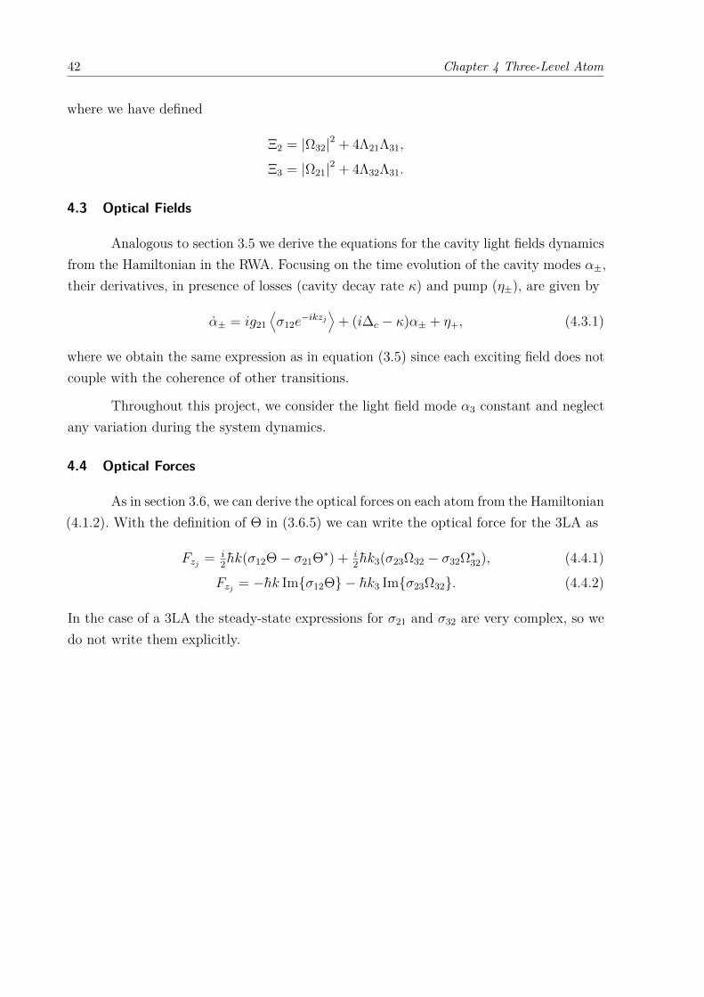
4.3 Optical Fields
Analogous to section 3.5 we derive the equations for the cavity light fields dynamicsfrom the Hamiltonian in the RWA. Focusing on the time evolution of the cavity modes α±,their derivatives, in presence of losses (cavity decay rate κ) and pump (η±), are given by
α± = ig21⟨σ12e
−ikzj
⟩+ (i∆c − κ)α± + η+, (4.3.1)
where we obtain the same expression as in equation (3.5) since each exciting field does notcouple with the coherence of other transitions.
Throughout this project, we consider the light field mode α3 constant and neglectany variation during the system dynamics.
4.4 Optical Forces
As in section 3.6, we can derive the optical forces on each atom from the Hamiltonian(4.1.2). With the definition of Θ in (3.6.5) we can write the optical force for the 3LA as
Fzj= i
2 hk(σ12Θ− σ21Θ∗) + i2 hk3(σ23Ω32 − σ32Ω∗32), (4.4.1)
Fzj= −hk Imσ12Θ − hk3 Imσ23Ω32. (4.4.2)
In the case of a 3LA the steady-state expressions for σ21 and σ32 are very complex, so wedo not write them explicitly.

43
5 ELECTROMAGNETIC INDUCED TRANSPARENCY - EIT
In this chapter, we focus on the optical properties of atomic clouds and discusshow they can be tuned taking advantage of the third level of the atoms.21–23
By inducing atomic coherences with a laser, we can cause quantum interferencebetween the different pathways in the energy level structure, which affects the materialoptical response. This way, it is actually even possible to reduce or even eliminate theabsorption of a transition. This phenomenon, called electromagnetic induced transparency(EIT), was demonstrated for the first time in a strontium gas24 where, by applying a strongcoupling field between a metastable state and the upper state of a permitted transition, itwas possible to obtain induced transparency in the material.
The main objective of studying this effect in our system is the intrinsic relationbetween the optical forces exerted by the light fields on the atoms and its transitioncoherences as in equations (4.4.2). Our objective is to understand if the manipulation ofthe atomic coherences could lead to a reduction in the radiative pressure force exerted onthe atoms.
5.1 Static description of EIT
To observe the EIT phenomenon, one needs at least two different transitions, as ina three-level system analysed in chapter 4. By making the distinction between the similarphenomenon of AT (Autler-Townes splitting),25 we can only select between a Lambda andCascade configuration to study the EIT. In this work we choose the Cascade.
Let us consider the trapped atomic cloud inside the ring cavity, interacting with
∆21
∆32
Γ31
Γ32
Γ21
|1〉
|2〉
|3〉
Ω32
Ω21
Figure 12 – Schematic representation of the Cascade three-level level system with thetransitions (blue and green arrows) excited by the light fields Ω21 and Ω32, andthe spontaneous decay transitions (red arrows) with respective decay ratesΓ21,Γ32,Γ31, where the last one can be neglected in our system.
Source: By the author.

44 Chapter 5 Electromagnetic Induced Transparency - EIT
two light field (E21 and E32), as described in equation (4.1.1). The interaction Hamiltonianfor this system can be written in the RWA as
Hint = h
2
0 Ω∗21 0
Ω21 2∆21 Ω∗32
0 Ω32 2(∆21 + ∆23)
, (5.1.1)
whose parameters were defined in chapter 4.
Although diagonalizing the Hamiltonian in the general case leads to complexexpressions, in the resonant case ∆21 +∆23 = 0 it is straightforward to obtain the followingeigenvalues
hω0 = 0, (5.1.2)
hω+ = ∆21 +√
∆221 + |Ω21|2 + |Ω32|2, (5.1.3)
hω− = ∆21 −√
∆221 + |Ω21|2 + |Ω32|2, (5.1.4)
which are associated to the following eigenstates:
|0〉 = Ω∗23Ω |1〉 − Ω12
Ω |3〉 , (5.1.5)
|+〉 = Ω∗12Ω sin θ |1〉+ cos θ |2〉+ Ω23
Ω sin θ |3〉 , (5.1.6)
|−〉 = Ω∗12Ω cos θ |1〉 − sin θ |2〉+ Ω23
Ω cos θ |1〉 , (5.1.7)
where we have introduced θ such as
sin 2θ =
√|Ω21|2 + |Ω32|2√
∆221 + |Ω21|2 + |Ω32|2
, (5.1.8)
cos 2θ = ∆12√∆2
21 + |Ω21|2 + |Ω32|2. (5.1.9)
State |0〉 is called a dark state since it does not interact with the light fields, i.e., it is notcoupled to the atomic eigenstate |2〉. This provides a basic understanding of the EIT: thedriven field sends the atom to a dark state, where an interaction with the probe light isno longer possible. As a result, it behaves as a transparent medium.
However, this description is oversimplified since it disregards the influence ofspontaneous emission, whose treatment requires a density matrix formalism as derived inchapter 4.
5.2 EIT in presence of spontaneous emission
The steady state solutions for the 3LA coherences (density matrix off-diagonalelements) were obtained in section 4.2. In this chapter we focus only on the coherence

5.2 EIT in presence of spontaneous emission 45
σ12 of the |1〉 → |2〉 transition. Although its expression is cumbersome, we can simplifyequation (4.2.2a) by considering that the transition |2〉-|3〉 is driven at resonance (∆32 = 0),and by neglecting the excited populations (ρ22 ≈ ρ33 ≈ 0):
σ12 = −iΩ21Ξ3
(Γ23 + Γ21)|Ω32|2 + (Γ21 + 2i∆21)Ξ3,
σ12 = −iΩ21|Ω32|2
|Ω21|2(Γ23+Γ21) +2Λ21
+ 2Λ21, (5.2.1)
where Ξ3 = |Ω21|2 +(Γ23 +Γ21)(Γ21 +2i∆21). Finally, since we considered that the transitionbetween levels |1〉 and |3〉 is prohibited, this allow us to neglect its decay rate, Γ31 = 0.Comparing to the case where Ω32 = 0, we can expect new resonant peaks in both real andimaginary parts of σ12, as can be observed in Fig. 13: it depicts the real and imaginarypart of σ12 as a function of the detuning for transition |1〉-|2〉, for different ratios betweenthe Rabi frequencies, Ω32/Ω21.
-4 -2 0 2 4
-1
-0.5
0
0.5
1
0
2
5
-4 -2 0 2 4
0
0.5
1
1.5
2
Figure 13 – Real and imaginary parts of the 3LA coherence σ12 as a function of thedetuning of the transition |1〉 → |2〉 for different pumping strengths Ω32 oftransition |2〉 → |3〉. Parameters for the figure are Γ32 = 0.1Γ21 and Ω21 = Γ21.
Source: By the author.
As expected, the curves for Ω32 = 0 in Fig. 13 are the same as those of the dipolarand radiative pressure forces in 3.6, since we recover the two-level atom case. The behaviorof the coherence near resonance is what instigates us to analyse the EIT phenomenon,since at high ratios of Ω32/Ω21 the imaginary part of σ12 (related to the radiative pressureforce), reaches lower values than the real part (related to the dipolar force). However, thesenew peaks only occur when the decay rate Γ32 is smaller than Γ21, and the resonances forσ21 only get broader, see Fig. 14, since the third level decays rapidly after being excitedfrom the second level, and the system behaves as a two-level atom.

46 Chapter 5 Electromagnetic Induced Transparency - EIT
-4 -2 0 2 4
-1
-0.5
0
0.5
1
0
2
5
-4 -2 0 2 4
0
0.5
1
1.5
2
Figure 14 – Real and imaginary parts of the 3LA coherence σ12 as a function of thedetuning of the transition |1〉 → |2〉 for different pumping strengths Ω32 oftransition |2〉 → |3〉. Parameters for the figure are Γ32 = 10Γ21 and Ω21 = Γ21.
Source: By the author.
Since the assumption of negligible excited populations is not valid for the near-resonance regime (Ω2
21/(Γ221 + 4∆2
21) not negligible ), we analyse the system using thefull optical Bloch equations (4.2.2) for the steady state. In Fig. 15 we reproduce the newresonant peaks and gaps in the coherence as in Fig. 13 at higher values of Ω21, throughouta larger region of ∆21.
-40 -20 0 20 40
21/
21
-0.4
-0.2
0
0.2
0.4
0
2
5
-40 -20 0 20 40
21/
21
0
0.01
0.02
0.03
0.04
0.05
-40 -20 0 20 40
21/
21
0
0.1
0.2
0.3
0.4
0.5
22
33
Figure 15 – Real and imaginary parts of the coherence σ12 as a function of the detuningfor the complete steady state Bloch equations and excited levels populations.Parameters for the figure are Γ32 = Γ21 and Ω21 = 10Γ21. In the right picture,for Ω32/Ω12 = 0, ρ33 = 0 (i.e., the dash-dotted blue curve overlaps with thex-axis)
Source: By the author.
For a decay rate Γ32 lower than Γ21 the imaginary part of σ12 reaches values closerto zero, see figure 16. This effect is not captured by equation (5.2.1), which neglects the

5.3 Radiative pressure force reduction 47
excited populations.
Figure 16 – Real and imaginary parts of the coherence σ12 as a function of the detuningfor the complete steady state Bloch equations and excited levels populations.Parameters for the figure are Γ32 = 0.1Γ21 and Ω21 = 10Γ21.
Source: By the author.
The most interesting characteristic of the depicted curves is that for a large ratiobetween the light field strengths, the real part of σ12 decays slower than the imaginarypart near the resonance, as it happens in the far-from-resonance regime for any value ofΩ32. This means that the dipolar force influence in the atomic dynamics can be strongerthan the radiative pressure force near resonance due to the EIT.
We also note that the excited populations are largely reduced near resonance, seeright graphic in Fig. 16 (i.e., at large detunings, the dipolar force dominates over theradiation pressure one). Such behavior can be exploited in the context of the adiabaticelimination, where the excited levels are eliminated from the dynamics when the light fieldis far detuned. Our results suggest that this effect can be achieved close to resonance usingthe EIT scheme.
5.3 Radiative pressure force reduction
From the above results we can infer that in the EIT regime the imaginary part ofσ12 is reduced in relation to its real part. Since from equation (3.6.4) we can associatethe imaginary and real part of the coherence with the radiative pressure and dipolarforce, respectively, therefore we can expect a large ratio between these forces near theresonance of transition |1〉-|2〉. However, it is only possible to obtain values of the ratio|Reσ12/ Im σ12| greater than the usual ratio (i.e., in absence of third level: Ω32 = 0), whenthe decay rate Γ32 is lower than Γ21. In Fig. 17 we can note that for Γ32/Γ21 = 10, theratio resembles a parabola, which is due to the absence of the resonant peaks in this case,as in Fig. 14.

48 Chapter 5 Electromagnetic Induced Transparency - EIT
-25 -20 -15 -10 -5 0 5 10 15 20 25
12/
21
0
20
40
60
80
100
120
1e+01
1e+00
1e-01
1e-02
Figure 17 – Ratio between real and imaginary parts of the transition |1〉-|2〉 coherence,varying the values of the decay rate for the transition |2〉-|3〉. Here we haveused Ω32 = 5Ω21 and Ω21 = 5Γ21. The black dashed line is the solution forΩ23 = 0.
Source: By the author.
Using equation (4.4.2) we can analyse the influence of EIT on the optical forces,analogously to the analysis made for the coherence in the previous section. By consideringdifferent atomic positions and different values for the counterpropagating cavity modesas in expression (3.6.8), it is possible to calculate separately the dipolar and radiativepressure forces.
-60 -40 -20 0 20 40 60
-3
-2
-1
0
1
2
310
7 Dipolar force
-60 -40 -20 0 20 40 60
0
0.5
1
1.5
2
2.5
3
3.510
6Radiative pressure force
Figure 18 – New resonant peaks in the optical forces steady state solutions, as functions ofthe transition |1〉-|2〉 detuning for different transition |2〉-|3〉 Rabi frequencies.Parameters for the figure are Γ32 = 0.1Γ21 and Ω12 = 10Γ21.
Source: By the author.

5.3 Radiative pressure force reduction 49
Figure 19 – Optical forces in hk as function of transition |1〉-|2〉 detuning and pumpstrength of transition |2〉-|3〉. Parameters for the figures are Γ32 = 0.5Γ21 andΩ12 = 10Γ21.
Source: By the author.
In Fig. 18 we present the new resonant peaks for each optical force obtained bythe steady state solution of σ12. Near resonance, we obtain a dipole force larger than theradiative pressure for large value of Ω32/Ω21, along with an inversion of sign related to thedetuning ∆21, which means that the forces becomes repulsive in a region where it wouldbe attractive without the EIT. Increasing the value o Ω32 we can see that those peaksgrow apart for both forces, see Fig. 19, where we calculate each force as a function of both∆21 and Ω32.
We determine the regions where the radiative pressure force is reduced enough soits dissipative effect on the atoms is lower than the dynamical effect of the dipolar force,by monitoring the ratio between those force |Fdip/Frad|. In Fig. 20 we can note that largevalues of this ratio are available near-resonance in the EIT regime, while such values wouldoccur only at far resonance regions without the pumping of transition |2〉-|3〉 (yet far fromresonance, the forces are much weaker). In Fig. 21 we show the forces ratio for a weakerlight-atom coupling Ω21 of transition |1〉-|2〉, which requires a lower decay rate and higherpump strength of transition |2〉-|3〉 to suppress the radiative pressure force.
50 Chapter 5 Electromagnetic Induced Transparency - EIT
Figure 20 – Ratio between dipolar and radiative force as function of transition |1〉-|2〉detuning and pump strength of transition |2〉-|3〉. Parameters for the figureare Γ32 = 0.1Γ21 and Ω12 = 10Γ21.
Source: By the author.
Figure 21 – Ratio between dipolar and radiative force as function of transition |1〉-|2〉detuning and pump strength of transition |2〉-|3〉. Parameters for the figureare Γ32 = 0.01Γ21 and Ω12 = 1Γ21.
Source: By the author.

51
6 MATTER-WAVES AND REPRESENTATION IN MOMENTUM SPACE
In the previous chapters we have showed that the EIT effect depends only on theinternal atom dynamics, which so far has allowed us to analyse the system equations usingonly its internal degrees of freedom. However, it is now necessary to consider extendedatoms to observe the Bloch oscillations, where the exchange of momentum between atomsand light fields occur at integers values of photon momentum.
In this chapter we introduce this formalism using the quantization of the momentumoperator, considering an atomic matter wave, and derive the optical Bloch equations forthe two- and three-level atom systems, including the optical lattice and external force asrequired to observe the Bloch oscillations.
6.1 Quantum momentum operator
The Hamiltonian of the atomic matter wave interacting with two different lightfields, within the dipole approximation and RWA, consists of the following contributions
Hatom = p2
2mo
− h∆21σ21σ12 − h∆32σ32σ23, (6.1.1a)
Hint = hg21(a†+e
−ikz + a†−eikz)σ12 + hg32a
†3e−ik3zσ23 + h.c., (6.1.1b)
Hfield = −h∆ca†qaq, (6.1.1c)
where gij = dijEij/2h is the light-atom coupling strength, also called the single-photonRabi frequency.
If the atomic sample is much larger than the radiation wavelength, and its densityis uniform, the atomic wave function Ψ(r, t) can be expanded into plane waves in thecavity axis z, with periodicity of kz
Ψ(r, t) =∑n
∑j
cj,nψj(r)einkz, (6.1.2)
where ψj are the unperturbed Hamiltonian eigenstates, and |cj,n|2 the probability of findingthe atoms in the n-th momentum state and j-th atomic state (j = 1, 2, 3 for a three-levelsystem).
The momentum quantization along the z-axis is realized by the definition of themomentum operator p, whose expectation value only assumes integer multiples of hk:
pz =∑n
nhk |n〉〈n| , (6.1.3)

52 Chapter 6 Matter-waves and representation in momentum space
where 〈r|n〉 = einkz is the momentum eigenstate. From the momentum and positioncommutator [z, p] = ih, we can derive the momentum kick-operator as
eikz =∑n
|n+ 1〉〈n| , e−ikz =∑n
|n− 1〉〈n| . (6.1.4)
Using the Dirac notation we can rewrite the atomic wave function as
|Ψ(t)〉 =∞∑
n=−∞
3∑j
cj,n |j, n〉 , (6.1.5)
where |j, n〉 = |j〉 ⊗ |n〉 , and 〈r|j〉 = ψj(r) is the atomic Hamiltonian eigenstate. Thenormalization condition of |Ψ〉 gives us the atoms number N in the matter wave as
〈Ψ(t)|Ψ(t)〉 = N. (6.1.6)
We can add the optical lattice contribution to the system through the term hWo sin(2kz)/2,which describes a stationary wave with periodicity of 2kz. This stationary wave can begenerated by two laser beams crossing the cavity at a determined angle, see Fig. 4.Expanding the sine,
Hlatt = hWo
2 sin(2kz) = −ihWo
4(e2ikz − e−2ikz
), (6.1.7)
we can see that the optical lattice contribution to the system are the momentum kickoperators, which change the atoms momentum in integers values of ±2hk.
The gravity force acting on the atoms can be included in the atomic Hamiltonian(6.1.1a) by potential V (r) = mogr, where r is the atom position operator and g is thegravity acceleration. To simplify the equations we consider the movement of the atom onlyin the z direction and describe the dynamics of the system in a accelerated frame movingwith momentum mogt in the positive direction of the z-axis. The atom wave-function inthis frame is transformed as
Ψ = Ψeimogzt/h, (6.1.8)
which is given by the free-fall solution of Ψ in this potential. The Schrödinger equation forthe atomic wave-function then reads
ihdΨdt = HatomΨ, (6.1.9)
ihdΨdt e
imogzt/h −mogzΨ = − h2k2
2mo
∂2
∂z2
(Ψeimogzt/h
)−mogzΨ, (6.1.10)
ihdΨdt = − h
2k2
2mo
(∂
∂z+ imogt
h
)2
Ψ. (6.1.11)
Finally the atomic Hamiltonian in the accelerated frame can be written as
Hatom = − h2k2
2mo
(p
hk+ imogt
h
)2
. (6.1.12)

6.2 Schrödinger equation for the two-level atoms 53
6.2 Schrödinger equation for the two-level atoms
We can start analysing the system for the two-level atom case in the Schrödingerequation picture by neglecting the spontaneous emission. The derivatives of the complexamplitudes in eq. (6.1.2) turn into the following set of coupled differential equations
c1,n = −iωr(n+ 2νbt)2c1,n + ig21(α∗+c2,n+1 + α∗−c2,n−1
)+ Wo
4 (c1,n+2 − c1,n−2), (6.2.1a)
c2,n = −iωr(n+ 2νbt)2c2,n − i∆21c2,n + ig21(α+c1,n−1 + α−c1,n+1) + Wo
4 (c2,n+2 − c2,n−2),(6.2.1b)
where ωr = hk2/2mo is the single-photon recoil frequency and νb = mog/hk is the Blochoscillation frequency.
As for the light field modes, using the Heisenberg equation and adding decay ratesfor the cavity κ and pump rates η±, we get
α± = (i∆c − κ)α± + ig21∑n
c∗1,n∓1c2,n + η±, (6.2.2)
where the atoms number can be recovered from the complex amplitudes from the nor-malization condition (6.1.6). The atomic movement can be described by the momentumoperator expectation value:
p = hk∑n
n(|c1,n|2 + |c2,n|2
), (6.2.3)
whose derivative, corresponding to the dipolar force, is given by
p = ihkg21∑n
([α∗+c∗1,n−1c2,n − α∗−c∗1,n+1c2,n]− c.c.
). (6.2.4)
We can see in Fig. 22 that the momentum modes populations for the atomic groundstates performs the Bloch oscillations due to the optical lattice and external force, and itsinteraction with the cavity mode α+ carries information about the atoms motions. Thesimulation was performed for a constant light field mode α− = η−/κ.
However, for low values of detuning for transition |1〉-|2〉 the excited level startsto influence on the Bloch oscillations, see Fig. 23. The pulses from the light field modeare damped due to the decoherence in the ground state population ∑n |c1n|2. Due to thelarge number of momentum states involved, numerical solutions become very complex andtime-consuming when considering the case of a light field far detuned from the atomicresonance (∆21 g21), since one has to deal with many fast oscillations between theatomic level states. To tackle this issue, we can perform an adiabatic elimination of theexcited state. When the light fields are very detuned from atomic resonances, the internaland external dynamics occur at very different time scales, where the former varies fasterand adapt very rapidly to the boundary conditions defined by the external state and the

54 Chapter 6 Matter-waves and representation in momentum space
0 1 2 3 4 5 6
0
0.5
1
0 1 2 3 4 5 6
0
20
40
60
Figure 22 – Time evolution of (top) the momentum modes populations of the atomicground state, where each color correspond to a momentum mode of evenn, and (bottom) the light field mode α+ intensity. Parameters used for thesimulation: g21 = 0.1ωr, α− = 1.25, ∆21 = 400ωr, ∆c = 0, κ = 160ωr andνb = 0.035ωr with N = 4.104 atoms.
Source: By the author.
light field. Therefore, the internal state has no dynamics on the time-scale of the atommotion, and we can adiabatically eliminate the internal degrees of freedom related to theatomic energy levels. Then the coherence between levels transition σ21 and populationsdifference D reaches the steady-states solutions as derived in section 3.4. Considering thecase without spontaneous emissions the solution for the coherence is given by
σ21(∞) = i
2Ω21∆21
|Ω21|2 + 2∆221≈ i
2g21(a+e
ikz + a−e−ikz)
∆21, (6.2.5)
where the approximation is performed in the regime where ∆221 |Ω21|2. Inserting the
above equation in equations (6.1.1), we obtain the Hamiltonian for the adiabatic eliminationof the excited state without pump
H = Hatom −ihg2
21∆21
(a†+e
−ik1z + a†−eik1z
)(a+e
ikz + a−e−ikz) + h∆ca
†±a± + hWo
2 sin(2kz),
(6.2.6)
H = Hatom − ihUo(a†+a−e
−2ik1z + a†−a+e2ik1z
)+ h(Uo−∆c)a†±a± + hWo
2 sin(2kz),
(6.2.7)
where Uo = g221/∆21 is the pump-probe coupling strength.
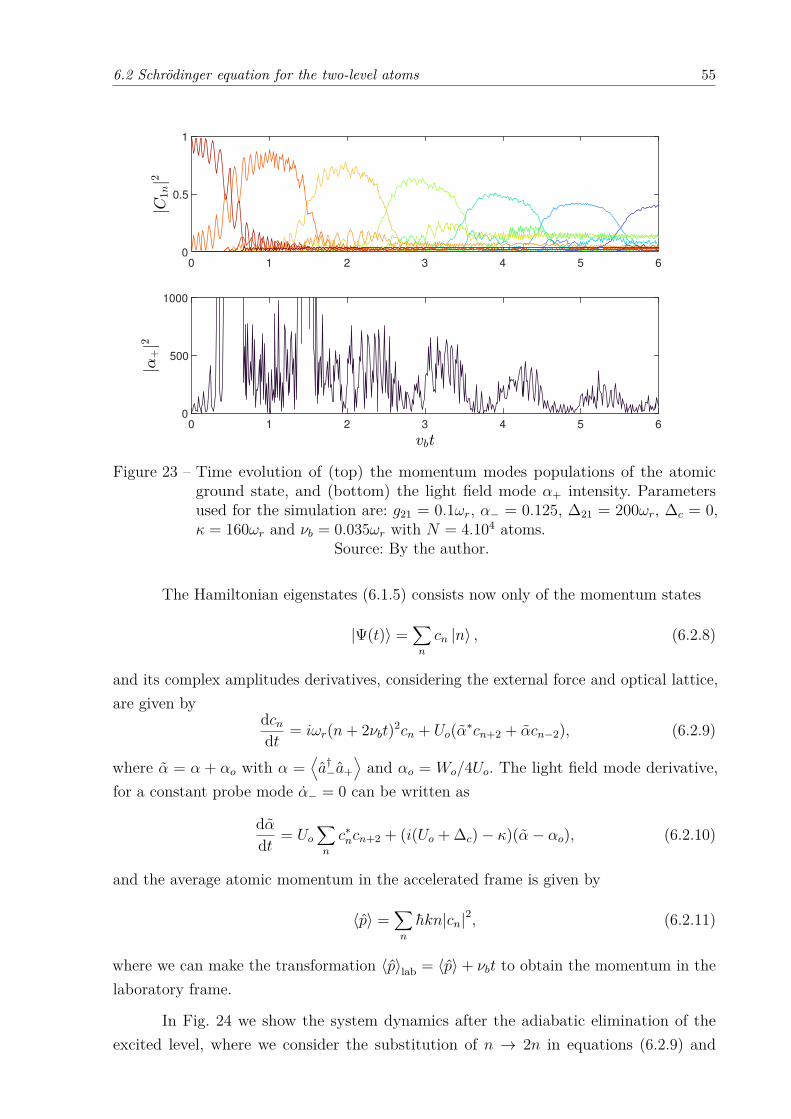
6.2 Schrödinger equation for the two-level atoms 55
0 1 2 3 4 5 6
0
0.5
1
0 1 2 3 4 5 6
0
500
1000
Figure 23 – Time evolution of (top) the momentum modes populations of the atomicground state, and (bottom) the light field mode α+ intensity. Parametersused for the simulation are: g21 = 0.1ωr, α− = 0.125, ∆21 = 200ωr, ∆c = 0,κ = 160ωr and νb = 0.035ωr with N = 4.104 atoms.
Source: By the author.
The Hamiltonian eigenstates (6.1.5) consists now only of the momentum states
|Ψ(t)〉 =∑n
cn |n〉 , (6.2.8)
and its complex amplitudes derivatives, considering the external force and optical lattice,are given by
dcndt = iωr(n+ 2νbt)2cn + Uo(α∗cn+2 + αcn−2), (6.2.9)
where α = α + αo with α =⟨a†−a+
⟩and αo = Wo/4Uo. The light field mode derivative,
for a constant probe mode α− = 0 can be written as
dαdt = Uo
∑n
c∗ncn+2 + (i(Uo + ∆c)− κ)(α− αo), (6.2.10)
and the average atomic momentum in the accelerated frame is given by
〈p〉 =∑n
hkn|cn|2, (6.2.11)
where we can make the transformation 〈p〉lab = 〈p〉+ νbt to obtain the momentum in thelaboratory frame.
In Fig. 24 we show the system dynamics after the adiabatic elimination of theexcited level, where we consider the substitution of n → 2n in equations (6.2.9) and

56 Chapter 6 Matter-waves and representation in momentum space
0 1 2 3 4 5 6 7 8 9
0
0.5
1
n = -10
n = -9
n = -8
n = -7
n = -6
n = -5
n = -4
n = -3
n = -2
n = -1
n = 0
0 1 2 3 4 5 6 7 8 9
-0.5
0
0.5
0 1 2 3 4 5 6 7 8 9
0
5
10
Figure 24 – Time evolution of (top) the momentum modes populations in the adiabaticelimination regime, (middle) the average atomic momentum in the laboratoryreference frame with N = 2.104 atoms and (bottom) the light field modeintensity. Parameters used for the simulation are: |αo| = 20, νb = 0.035ωr,Uo = 0.04ωr, ∆c = 0 and κ = 160ωr.
Source: By the author.
(6.2.10), since the dynamics occurs only at even numbers of n. Neglecting the oscillationsbetween atomic level states allows us to observe more momentum modes oscillations witha reduced integration time of the numerical routine.
In fact we are able to observe the CARL dynamics dominating the system for a largeatoms number in Fig. 25, and for a large cooperative coupling NUo/κ, which manifests aspulses of backscattered photons in the mode α and the acceleration in the average atomicmomentum. This can be explained as a scattering of photons from the pumped cavitymode into the reverse mode α, which influence the atoms dynamics. In this regime, themomentum transfer from the fields to the atoms results in the backscattering of the pumplight by a self-generated atomic density grating. As a consequence, the population transferbetween adjacent momentum states does not occur at the regular Bloch periods νb.8,9
However, such behavior can not be reproduced by solving equations (6.2.1), sinceit would require a large detuning to maintain the atoms in the ground state, which in turnis very costly from a numerical standpoint.
6.3 Master equation for the three-level atoms
Let us now derive complete equations from the three-level system. We start bydefining the system density matrix regarding the internal and external atomic degrees

6.3 Master equation for the three-level atoms 57
0 0.5 1 1.5 2 2.5
0
0.5
1
n = -10
n = -9
n = -8
n = -7
n = -6
n = -5
n = -4
n = -3
n = -2
n = -1
n = 0
0 0.5 1 1.5 2 2.5
-6
-4
-2
0
0 0.5 1 1.5 2 2.5
0
200
400
Figure 25 – Time evolution of (top) the momentum modes populations, (middle) theaverage atomic momentum in the laboratory reference frame with N = 12.104
atoms and (bottom) the light field mode intensity for the system dominatedby CARL dynamics. Parameters used for the simulation are similar to Fig. 24
Source: By the author.
of freedom. To simplify our equations we consider that both light fields have similarwave-numbers k1 ≈ k3 ≈ k.
Within the rotating wave approximation we can write the density matrix for theatomic system
ρ(t) = |Ψ(t)〉〈Ψ(t)| , (6.3.1)
ρm,nij = 〈i,m| ρ |j, n〉 . (6.3.2)
The equations of motion for the density matrix element is given by the von Neumannequation with the Hamiltonian (6.1.1) and the dissipative term of the Lindblad super-operators:
dρdt = i
h[ρ,H] + Latomρ+ Lcavityρ, (6.3.3)
which write
Latomρ = −∑i,j
γij(σjiσij ρ− 2σij ρσji + ρσjiσij), (6.3.4)
Lcavρ = −κ(a†±a±ρ− 2a±ρa†± + ρa†±a±
). (6.3.5)
Then, the derivative of each density matrix element is written as
ρm,nij = i
h〈i,m| [ρ,Hatom +Hint] |j, n〉+ 〈i,m| Latomρ |j, n〉 . (6.3.6)

58 Chapter 6 Matter-waves and representation in momentum space
Expanding the first term in the RHS of the above expression (denominated the coherentpart), we obtain
〈i,m| [ρ,Hat,int] |j, n〉 = 〈i,m| ρ∑v,q
|v, q〉〈v, q|Hat,int |j, n〉
− 〈i,m|Hat,int
∑u,p
|u, p〉〈u, p| ρ |j, n〉 , (6.3.7)
〈i,m| [ρ,Hat,int] |j, n〉 =∑v,q
ρm,qi,v 〈v, q|Hat,int |j, n〉 −∑u,p
〈i,m|Hat,int |u, p〉 ρp,nu,j , (6.3.8)
〈i,m| [Hat,int, ρ] |j, n〉 = h
[(n2 −m2)hk2
2mo
−∆21(δj2 − δi2)−∆32(δj3 − δi3)]ρm,nij
− hg21[α∗+(δi1ρ
m+1,n2j − δj2ρm,n−1
i1
)+ α∗−
(δi1ρ
m−1,n2j − δj2ρm,n+1
i1
)]− hg21
[α+(δi2ρ
m−1,n1j − δj1ρm,n+1
i2
)+ α−
(δi2ρ
m+1,n1j − δj1ρm,n−1
i2
)]− hg32α
∗3
(δi2ρ
m+1,n3j − δj3ρm,n−1
i2
)− hg32α3
(δi3ρ
m−1,n2j − δj2ρm,n+1
i3
). (6.3.9)
As for the incoherent part of equation (6.3.6), one gets
〈i,m| Latomρ |j, n〉 = −∑k,l
〈i,m| γkl(σlkσklρ− 2σklρσlk + ρσlkσkl) |j, n〉 , (6.3.10)
〈i,m| Latomρ |j, n〉 = −∑k,l
〈i,m| γklσlkσkl∑u,p
|u, p〉〈u, p| ρ |j, n〉
+ 2∑k,l
γkl 〈i,m| σkl∑u,p
|u, p〉〈u, p| ρ∑v,q
|v, q〉〈v, q| σlk |j, n〉
−∑k,l
γkl 〈i,m| ρ∑u,p
|u, p〉〈u, p| σlkσkl |j, n〉 , (6.3.11)
〈i,m| Latomρ |j, n〉 =∑k,l
∑u,p,q,v
2γkl 〈i,m| σkl |u, p〉 ρp,qu,v 〈v, q| σlk |j, n〉
−∑k,l,u,p
γkl 〈i,m| σlkσkl |u, p〉 ρp,nu,j −∑k,l,u,p
γklρm,pi,u 〈u, p| σlkσkl |j, n〉 , (6.3.12)
〈i,m| Latomρ |j, n〉 =∑k,l
2δi,kδjkγklρm,nl,l −∑k
(γki + γkj)ρm,nij . (6.3.13)
Gathering all the equations we obtain from the following derivative for the densitymatrix elements
ρm,nij = i
[hk2
2mo
(n2 −m2)−∆21(δj2 − δi2)−∆32(δj3 − δi3)]ρm,nij
− ig21[α∗+(δi1ρ
m+1,n2j − δj2ρm,n−1
i1
)+ α∗−
(δi1ρ
m−1,n2j − δj2ρm,n+1
i1
)]− ig21
[α+(δi2ρ
m−1,n1j − δj1ρm,n+1
i2
)+ α−
(δi2ρ
m+1,n1j − δj1ρm,n−1
i2
)]− ig32α
∗3
(δi2ρ
m+1,n3j − δj3ρm,n−1
i2
)− ig32α3
(δi3ρ
m−1,n2j − δj2ρm,n+1
i3
)+∑k,l
2δi,kδjkγklρm,nl,l −∑k
(γki + γkj)ρm,nij . (6.3.14)

6.3 Master equation for the three-level atoms 59
The derivatives for each element of the density matrix, after performing thetransformation into the driving fields frame 3.2.1, read
ρm,n11 = iωmnr ρm,n11 + Γ12ρm,n22 + Γ13ρ
m,n33
− ig21(α∗+σ
m+1,n21 + α∗−σ
m−1,n21 − α+σ
m,n+112 − α−σm,n−1
12
),
(6.3.15a)
ρm,n22 = iωmnr ρm,n22 − Γ12ρm,n22 + Γ23ρ
m,n33 − ig32
(α∗3σ
m+1,n32 − α3σ
m,n+123
)+ ig21
(α∗+σ
m,n−121 + α∗−σ
m,n+121 − α+σ
m−1,n12 − α−σm+1,n
12
),
(6.3.15b)
ρm,n33 = iωmnr ρm,n33 − (Γ23 + Γ13)ρm,n33 + ig32(α∗3σ
m,n−132 − α3σ
m−1,n23
), (6.3.15c)
σm,n21 = −(
Γ12
2 − i∆mn21
)σm,n21 + ig32α
∗3σ
m+1,n31
− ig21[α+(ρm−1,n
11 − ρm,n+122
)+ α−
(ρm+1,n
11 − ρm,n−122
)],
(6.3.15d)
σm,n31 = −(
Γ13
2 − i∆mn31
)σm,n31 + ig32α3σ
m−1,n21 − ig21
(α∗+σ
m,n+132 + α∗−σ
m,n−132
), (6.3.15e)
σm,n32 = −(
Γ23
2 − i∆mn32
)σm,n32 + ig21
(α∗+σ
m,n−131 + α∗−σ
m,n+131
)− ig32α3
(ρm−1,n
22 − ρm,n+133
),
(6.3.15f)
where ρij = σijeiω, ∆mn
ij = ωij + ωmnr − ω, ωnmr = (n2 −m2) hk2
2mois the recoil frequency for
a momentum transition from n to m and Γij = 2γij the linewidth of the respective atomiclevel transition. The phases eiωt are absorbed by the fields amplitudes α.
From the Heisenberg equation the fields equations of motion yields
α+ = (i∆c − κ)α+ − ig21∑n
σn−1,n12 + η+, (6.3.16a)
α− = (i∆c − κ)α− − ig21∑n
σn+1,n12 + η−. (6.3.16b)
The derivative for the density matrix element with the external force includes the term−2ihk2
mo(m − n)νbtρm,nij in 6.3.14, where νb = moa/2hk. In order to avoid repeating the
equations (6.3.15) we can include this term into the recoil frequency as
ωm,nr = hk2
2mo
[(n2 −m2) + 4(n−m)νbt
]. (6.3.17)
The corresponding terms in the density matrix elements derivatives from the optical latticeare given by the Hamiltonian in equation (6.1.7)
i
h[ρ,Hlatt] = −Wo
4[(e2ikz − e−2ikz
), ρ], (6.3.18)
〈i,m|[e±2ikz, ρ
]|j, n〉 = ρm∓2,n
ij − ρm,n±2ij , (6.3.19)
which can be added to equations (6.3.14) as
−Wo
4(ρm−2,nij − ρm,n+2
ij − ρm+2,nij + ρm,n−2
ij
). (6.3.20)

60 Chapter 6 Matter-waves and representation in momentum space
6.4 Results
In this section we present the obtained results for equations (6.3.15) in presence ofthe gravity and optical lattice. At first, we reproduce the dynamics for the 2LA as shownby Fig. 26, where the third level is “turned off” by setting g32 = 0.
0 1 2 3 4 5 6
0
1
2
3
0 1 2 3 4 5 6
0
0.5
1
11
nn
n = 0
n = -1
n = -2
n = -3
n = -4
n = -5
n = -6
n = -7
n = -8
n = -9
n = -10
n = -11
n = -12
0 1 2 3 4 5 6
-1
0
1
Figure 26 – (top) Bloch oscillations for a two-level atom by solving equations (6.3.15)with g32 = 0, (middle) average atomic momentum in the laboratory referenceframe (in hk) with N = 4.104 atoms and (bottom) time evolution of thelight field mode intensity. Parameters used for the simulation are: α− = 102,νb = 0.035ωr, Uo = 0.04ωr, ∆c = 0, κ = 160ωr, ∆21 = 50ωr and g21 = 0.1ωr.
Source: By the author.
The main interest of solving the master equation for this system is to include thedissipation effect of the spontaneous emission. In Fig. 27 we can observe this effect onthe Bloch oscillations for a large detuning ∆21 = 2.103Γ21. The decoherence on the atomsdynamics occurs as odd momentum modes of the ground state are populated (dashedlines in the figures). Those momentum modes come from the excited state, which decaysaccording to the term Γ21ρ
m,n22 in equation (6.3.15b).
For the dynamics, it is required to include positive momentum modes in thenumerical routine. A full spectrum of n would show that those momentum modes arealso populated throughout the system dynamic, but this effect is rather weak, as canbe summarized in the mode n = 2, see Fig. 27 and 28.26 The atoms in those modes areeliminated from the cloud since they are accelerated towards gravity, and their influenceon the light fields are negligible for small decay rates.
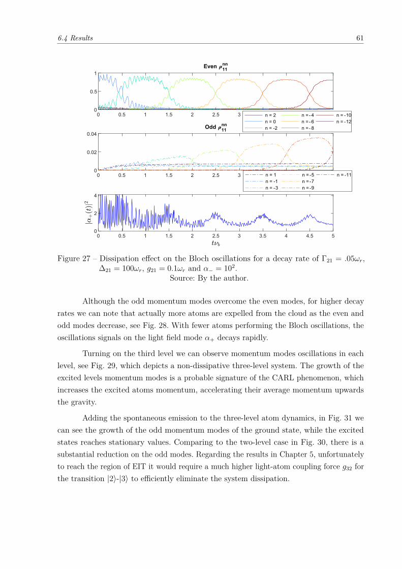
6.4 Results 61
Figure 27 – Dissipation effect on the Bloch oscillations for a decay rate of Γ21 = .05ωr,∆21 = 100ωr, g21 = 0.1ωr and α− = 102.
Source: By the author.
Although the odd momentum modes overcome the even modes, for higher decayrates we can note that actually more atoms are expelled from the cloud as the even andodd modes decrease, see Fig. 28. With fewer atoms performing the Bloch oscillations, theoscillations signals on the light field mode α+ decays rapidly.
Turning on the third level we can observe momentum modes oscillations in eachlevel, see Fig. 29, which depicts a non-dissipative three-level system. The growth of theexcited levels momentum modes is a probable signature of the CARL phenomenon, whichincreases the excited atoms momentum, accelerating their average momentum upwardsthe gravity.
Adding the spontaneous emission to the three-level atom dynamics, in Fig. 31 wecan see the growth of the odd momentum modes of the ground state, while the excitedstates reaches stationary values. Comparing to the two-level case in Fig. 30, there is asubstantial reduction on the odd modes. Regarding the results in Chapter 5, unfortunatelyto reach the region of EIT it would require a much higher light-atom coupling force g32 forthe transition |2〉-|3〉 to efficiently eliminate the system dissipation.

62 Chapter 6 Matter-waves and representation in momentum space
0 0.5 1 1.5 2 2.5 3 3.5 4 4.5 50
1
2
0 0.5 1 1.5 2 2.5 3 3.5 4 4.5 50
0.5
1
Eve
n
11
nn
n = 2
n = 0
n = -2
n = -4
n = -6
n = -8
n = -10
n = -12
0 0.5 1 1.5 2 2.5 3 3.5 4 4.5 50
0.1
0.2
Od
d
11
nn
n = 1
n = -1
n = -3
n = -5
n = -7
n = -9
n = -11
Figure 28 – Dissipation effect on the Bloch oscillations for a decay rate of Γ21 = 2.5ωr,∆21 = 100ωr, g21 = 0.1ωr and α− = 102.
Source: By the author.
0 2 4 6
0
1
2
3
0 2 4 6
0
0.5
1
11
nn
0 2 4 6
0
0.005
0.01
0.01522
nn
0 2 4 6
0
0.005
0.01
0.01533
nn
n = 0
n = -1
n = -2
n = -3
n = -4
n = -5
n = -6
n = -7
n = -8
n = -9
n = -10
n = -11
n = -12
n = -13
n = -14
Figure 29 – Bloch oscillations on the three atomic levels without dissipation. Parametersfor the figure are: ∆21 = 50, Γ21 = Γ32 = 0, g21 = 0.1ωr and g32 = 10ωr.
Source: By the author.

6.4 Results 63
Figure 30 – Bloch oscillations on two atomic levels with dissipation. Parameters for thefigure are: ∆21 = 50, Γ21 = 0.05ωr, Γ32 = 0, g21 = 0.1ωr and g32 = 0ωr.
Source: By the author.
Figure 31 – Bloch oscillations on three atomic levels with dissipation. Parameters for thefigure are: ∆21 = 50, Γ21 = 0.05ωr, Γ32 = 0, g21 = 0.1ωr and g32 = 10ωr.
Source: By the author.

65
7 CONCLUSIONS
In the previous chapter, we derived the equations of motion for the three-levelatoms system interacting with light fields driving the two transitions. The contributionsof an optical lattice and the gravity force were considered, in order to combine theCARL phenomenon and the Bloch oscillations in the system, which required a plane waveexpansion of the atoms wave-function. With this, we considered entangled states thatcombined the atomic momentum mode and its internal energy level. We also considered anapproximation assuming the same wave-numbers for the two transitions, so that we couldanalyse the movement of the atoms in each level with the same plane wave expansion andin the same direction. Other configurations lead to a more complex form for the equationsof motion, where a much larger momentum space would be accessible to the atoms.27
The set of coupled differential equations for the density matrix elements and forthe coupled dynamics of the light field modes allows us to perform numerical routinesto simulate the atoms momentum dynamics over several Bloch oscillations. As we donot consider an adiabatic elimination of the excited levels, these equations involve morevariables than previous works.9 Thus, the obtained results are valid for small detuningand light-atom coupling strength. Using the master equation formalism, we were able toanalyse the influence of spontaneous emission on the Bloch oscillations. We showed thatthis dissipation phenomenon suppress the modes oscillations, while populating intermediatemodes that did not appear before in the ground state. Although one could expect thatthose intermediate mode oscillations would remain throughout the dynamics, they saturateand then decay. This decay is accompanied by the atoms stopping to interact with thelight, as the population of positive momentum modes (in the gravity reference frame)increases throughout the dynamics.
A possible solution to this problem would be the EIT, whose influence on thedissipative radiative pressure force was analysed in chapter 5. However, to reach theregion where this phenomenon is expected to occur, computational resources with highercapacities are required. Here we have presented results showing that even for a region wherethe radiative pressure is not efficiently suppressed, the dissipation of the momentum modesoscillations is reduced. Those preliminary results motivate us to continue the investigationof Bloch oscillations close to regions where the EIT influence on the system is substantial,with the adoption of more advanced numerical methods. The EIT in the Λ three-level atomconfiguration is also worth investigating, since our results show that the radiative pressureforce reduction relies on a condition between the decay rates of the levels transitions for acascade configuration, which limits the relevant atomic species.
An effect that can be better investigated is the dynamics considering a full spectrum

66 Chapter 7 Conclusions
of the momentum modes, as in recent works where two matter waves performing Blochoscillations were combined.26 This would allow the investigation of matter-wave performingBloch oscillations in a ring cavity, such that their interaction with the light field leads toan interference, which can carry extra information of the atoms motion.
———————————————————-

67
REFERENCES
1 MARSON, I. A short walk along the gravimeters path. International Journal ofGeophysics, Hindawi Limited, v. 2012, p. 1–9, 2012. DOI: 10.1155/2012/687813.
2 ROATI, G. et al. Atom interferometry with trapped fermi gases. Physical ReviewLetters, American Physical Society (APS), v. 92, n. 23, p. 230402, June 2004.
3 BLOCH, F. Uber die quantenmechanik der elektronen in kristallgittern. Zeitschriftfür Physik, Springer Science and Business Media LLC, v. 52, n. 7-8, p. 555–600, July1929.
4 DAHAN, M. B. et al. Bloch oscillations of atoms in an optical potential. PhysicalReview Letters, American Physical Society (APS), v. 76, n. 24, p. 4508–4511, June1996.
5 FERRARI, G. et al. Long-lived bloch oscillations with bosonic sr atoms and applicationto gravity measurement at the micrometer scale. Physical Review Letters, AmericanPhysical Society (APS), v. 97, n. 6, p. 060402, Aug. 2006.
6 GUSTAVSSON, M. et al. Control of interaction-induced dephasing of bloch oscillations.Physical Review Letters, American Physical Society (APS), v. 100, n. 8, p. 080404,Feb. 2008.
7 BATTESTI, R. et al. Bloch oscillations of ultracold atoms: a tool for a metrologicaldetermination of h/mrb. Physical Review Letters, American Physical Society, v. 92, p.253001, June 2004.
8 SAMOYLOVA, M. et al. Mode-locked bloch oscillations in a ring cavity. LaserPhysics Letters, IOP Publishing, v. 11, n. 12, p. 126005, Nov. 2014.
9 SAMOYLOVA, M. et al. Synchronization of bloch oscillations by a ring cavity. OpticsExpress, Optical Society of America, v. 23, n. 11, p. 14823, May 2015.
10 SAMOYLOVA, M. Stabilization of bloch oscillations of ultracold atoms in aring cavity. 2015. Tesi (Dottorato) — Università degli Studi di Milano, Milano, 2015.
11 GLUCK, M. et al. Calculation of wannier-bloch and wannier-stark states. TheEuropean Physical Journal D, Springer Science and Business Media LLC, v. 4, n. 3,p. 239–246, Dec. 1998.
12 LARSON, J. Level crossings in a cavity QED model. Physical Review A, AmericanPhysical Society (APS), v. 73, n. 1, p. 013823, Jan. 2006.
13 MAUNZ, P. et al. Cavity cooling of a single atom. Nature, Nature Publishing Group,v. 428, n. 6978, p. 50, 2004.
14 COURTEILLE, P. W. The collective atomic recoil laser. AIP ConferenceProceedings, v. 770, n. 1, p. 135, 2005.
15 KRUSE, D. et al. Observation of lasing mediated by collective atomic recoil. PhysicalReview Letters, APS, v. 91, n. 18, p. 183601, 2003.

68 References
16 ALLEN, L. Optical resonance and two-level atoms. New York: Wiley, 1975.ISBN 0471023272.
17 LOUDON, R. The quantum theory of light: Oxford: Oxford University Press,2000. ISBN 0198501765.
18 GERRY, C.; KNIGHT, P. Introductory quantum optics: Cambrigde: CambridgeUniversity Press, 2004.
19 MEYSTRE, P.; SARGENT, M. (ed.). Elements of quantum optics. Berlin:Springer Verlag, 2007.
20 MANZANO, D. A short introduction to the lindblad master equation. AIPAdvances, AIP Publishing, v. 10, n. 2, p. 025106, Feb. 2020.
21 HARRIS, S. E. Electromagnetically induced transparency. Physics Today, AIPPublishing, v. 50, n. 7, p. 36–42, July 1997.
22 FLEISCHHAUER, M.; IMAMOGLU, A.; MARANGOS, J. P. Electromagneticallyinduced transparency: optics in coherent media. Reviews of Modern Physics,American Physical Society (APS), v. 77, n. 2, p. 633–673, July 2005.
23 MARANGOS, J. P. Electromagnetically induced transparency. Journal of ModernOptics, Taylor & Francis, v. 45, n. 3, p. 471–503, Mar. 1998.
24 HARRIS, S. E.; FIELD, J. E.; IMAMOGLU, A. Nonlinear optical processes usingelectromagnetically induced transparency. Physical Review Letters, American PhysicalSociety, v. 64, n. 10, p. 1107–1110, Mar. 1990.
25 ABI-SALLOUM, T. Y. Eit and at: two similar but distinct phenomena in twocategories of three-level atomic systems. Physical Review A, American Physical Society(APS), v. 81, n. 5, p. 053836, May 2010.
26 PAGEL, Z. et al. Symmetric bloch oscillations of matter waves. Physical ReviewA, American Physical Society (APS), v. 102, n. 5, p. 053312, Nov. 2020.
27 BUX, S. et al. Control of matter-wave superradiance with a high-finesse ring cavity.Physical Review A, American Physical Society (APS), v. 87, n. 2, p. 023607, Feb. 2013.