Nonlinear Dyn (2013) 71:121–132DOI 10.1007/s11071-012-0645-2

O R I G I NA L PA P E R

Dynamics of microbubble oscillators with delay coupling

C.R. Heckman · R.H. Rand

Received: 10 July 2012 / Accepted: 11 October 2012 / Published online: 30 October 2012© Springer Science+Business Media Dordrecht 2012

Abstract Two vibrating bubbles submerged in a fluidinfluence each others’ dynamics via sound waves inthe fluid. Due to finite sound speed, there is a delaybetween one bubble’s oscillation and the other’s. Thisscenario is treated in the context of coupled nonlin-ear oscillators with a delay coupling term. It has previ-ously been shown that with sufficient time delay, a su-percritical Hopf bifurcation may occur for motions inwhich the two bubbles are in phase. In this work, wefurther examine the bifurcation structure of the cou-pled microbubble equations, including analyzing thesequence of Hopf bifurcations that occur as the timedelay increases, as well as the stability of this motionfor initial conditions which lie off the in-phase mani-fold. We show that in fact the synchronized, oscillatingstate resulting from a supercritical Hopf is attractingfor such general initial conditions.

CRH acknowledges the support of the National ScienceFoundation through the Graduate Research FellowshipProgram. Any opinions, findings, and conclusions orrecommendations expressed in this publication are those of theauthors and do not reflect those of the National ScienceFoundation.

C.R. HeckmanField of Theoretical and Applied Mechanics,Cornell University, Ithaca, NY 14850, USA

R.H. Rand (�)Department of Mechanical and Aerospace Engineeringand Department of Mathematics, Cornell University,Ithaca, NY 14850, USAe-mail: rhr2@cornell.edu

Keywords Microbubble · Differential delayequation · Perturbation theory · Hopf bifurcation

1 Introduction

Delay is a widely exhibited phenomenon in dynam-ical systems, characterized by when a system’s cur-rent state depends at least in part on its history. Thereare a wealth of examples of such systems, rangingfrom technological to biological. Coupled laser sys-tems, high-speed milling, population dynamics, andgene expression are just a handful of examples wherenonnegligible delay presents itself inherently in thedynamics of the system under study. This paper ex-amines a system of coupled microbubbles, which areinfluencing each other via acoustic waves. Such stud-ies are motivated in part by medical applications—inparticular, the localized delivery of drugs via bubbletransport. In this process, microbubbles filled with adrug are used as a vehicle for local delivery and arepropagated to a target site by use of ultrasound forcing[1, 3, 9]. In such a scenario, it is desirable to have acomplete picture of the dynamical behavior of inter-acting microbubbles in order to appropriately predicttheir motion, for instance, in a feedback system. Fullunderstanding of the behavior of systems of coupledmicrobubbles involves taking into account the speedof sound in the liquid, which will lead to a delay in in-duced pressure waves between the bubbles in a cloud.

122 C.R. Heckman and R.H. Rand

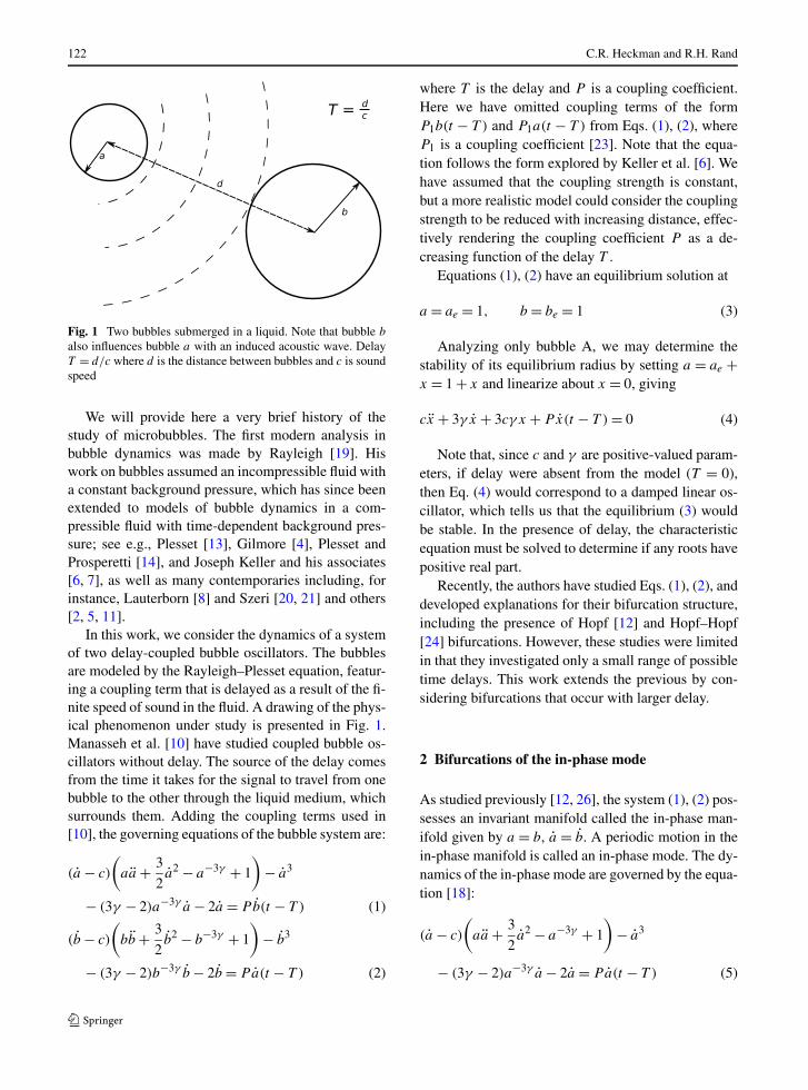
Fig. 1 Two bubbles submerged in a liquid. Note that bubble b

also influences bubble a with an induced acoustic wave. DelayT = d/c where d is the distance between bubbles and c is soundspeed

We will provide here a very brief history of thestudy of microbubbles. The first modern analysis inbubble dynamics was made by Rayleigh [19]. Hiswork on bubbles assumed an incompressible fluid witha constant background pressure, which has since beenextended to models of bubble dynamics in a com-pressible fluid with time-dependent background pres-sure; see e.g., Plesset [13], Gilmore [4], Plesset andProsperetti [14], and Joseph Keller and his associates[6, 7], as well as many contemporaries including, forinstance, Lauterborn [8] and Szeri [20, 21] and others[2, 5, 11].

In this work, we consider the dynamics of a systemof two delay-coupled bubble oscillators. The bubblesare modeled by the Rayleigh–Plesset equation, featur-ing a coupling term that is delayed as a result of the fi-nite speed of sound in the fluid. A drawing of the phys-ical phenomenon under study is presented in Fig. 1.Manasseh et al. [10] have studied coupled bubble os-cillators without delay. The source of the delay comesfrom the time it takes for the signal to travel from onebubble to the other through the liquid medium, whichsurrounds them. Adding the coupling terms used in[10], the governing equations of the bubble system are:

(a − c)

(aa + 3

2a2 − a−3γ + 1

)− a3

− (3γ − 2)a−3γ a − 2a = P b(t − T ) (1)

(b − c)

(bb + 3

2b2 − b−3γ + 1

)− b3

− (3γ − 2)b−3γ b − 2b = P a(t − T ) (2)

where T is the delay and P is a coupling coefficient.Here we have omitted coupling terms of the formP1b(t − T ) and P1a(t − T ) from Eqs. (1), (2), whereP1 is a coupling coefficient [23]. Note that the equa-tion follows the form explored by Keller et al. [6]. Wehave assumed that the coupling strength is constant,but a more realistic model could consider the couplingstrength to be reduced with increasing distance, effec-tively rendering the coupling coefficient P as a de-creasing function of the delay T .

Equations (1), (2) have an equilibrium solution at

a = ae = 1, b = be = 1 (3)

Analyzing only bubble A, we may determine thestability of its equilibrium radius by setting a = ae +x = 1 + x and linearize about x = 0, giving

cx + 3γ x + 3cγ x + P x(t − T ) = 0 (4)

Note that, since c and γ are positive-valued param-eters, if delay were absent from the model (T = 0),then Eq. (4) would correspond to a damped linear os-cillator, which tells us that the equilibrium (3) wouldbe stable. In the presence of delay, the characteristicequation must be solved to determine if any roots havepositive real part.

Recently, the authors have studied Eqs. (1), (2), anddeveloped explanations for their bifurcation structure,including the presence of Hopf [12] and Hopf–Hopf[24] bifurcations. However, these studies were limitedin that they investigated only a small range of possibletime delays. This work extends the previous by con-sidering bifurcations that occur with larger delay.

2 Bifurcations of the in-phase mode

As studied previously [12, 26], the system (1), (2) pos-sesses an invariant manifold called the in-phase man-ifold given by a = b, a = b. A periodic motion in thein-phase manifold is called an in-phase mode. The dy-namics of the in-phase mode are governed by the equa-tion [18]:

(a − c)

(aa + 3

2a2 − a−3γ + 1

)− a3

− (3γ − 2)a−3γ a − 2a = P a(t − T ) (5)

Dynamics of microbubble oscillators with delay coupling 123

We analyze the equilibrium of this equation a =ae = 1 for Hopf bifurcations, giving rise to oscilla-tions. When Hopf bifurcations occur, there will be achange in stability of the equilibrium point. To studythe stability of the equilibrium point, we will analyzeits linearization as provided in Eq. (4). This equationis a linear differential-delay equation. To solve it, weset x = expλt (see [15, 22]), giving

cλ2 + 3γ λ + 3cγ = −Pλ exp−λT (6)

We seek the values of delay T = Tcr, which causeinstability. This will correspond to imaginary valuesof λ. Thus, we substitute λ = iω in Eq. (6) giving tworeal equations for the real-valued parameters ω and T :

Pω sinωT = c(ω2 − 3γ

)(7)

Pω cosωT = −3γω (8)

Note that these equations have infinitely many so-lutions, as anticipated by the transcendental form ofEq. (6). In our previous work, only the first solutionwas studied. However, a further analysis of the bifur-cation structure involves analyzing the full solution setto Eqs. (7), (8). We choose the following dimension-less parameters based on the papers by Keller et al.when numerics are required:

c = 94, γ = 4

3, P = 10 (9)

The solutions to Eq. (6) are then found to be:

ωα =√

P 2 − 9γ 2 + 12c2γ + √P 2 + 9γ 2

2c≈ 2.0493

⇒ Tα = arccos (−3γ10 ) + 2πn

ωα

(n ∈ Z) (10)

ωβ =√

P 2 − 9γ 2 + 12c2γ − √P 2 + 9γ 2

2c≈ 1.9518

⇒ Tβ = − arccos (−3γ10 ) + 2πm

ωβ

(m ∈ Z) (11)

Notice that, while there are only two frequenciesωα , ωβ that solve the equations, each of them hasan infinite sequence of Tα , Tβ , respectively, that pairswith it as a solution. We will designate any delay T atwhich a Hopf bifurcation occurs as Tcr, independent ofits corresponding frequency. Because of the solutionsto Eqs. (7), (8) there will be two infinite sequences of

Fig. 2 Amplitude of limit cycle oscillations using numericalcontinuation of Eq. (5) for the parameter values in Eq. (9), withT as the continuation parameter. The Hopf bifurcations occurin a sequence where Tα is followed by Tβ , and the two limitcycles coalesce in a saddle node of periodic orbits. The plot iscontinued in Fig. 3

Fig. 3 Amplitude of limit cycle oscillations using numericalcontinuation of Eq. (5) for the parameter values in Eq. (9), withT as the continuation parameter. The Hopf bifurcations occur ina sequence where Tα is followed by Tβ until T ≈ 44, where twoTα -type Hopf bifurcations occur in a row. This is a continuationof Fig. 2

solutions that occur simultaneously. Each of the Tα ,Tβ delays correspond to Hopf bifurcations.

Using the numerical continuation package DDE-BIFTOOL [28], we present the amplitude of limit cy-cle oscillations that are born out of these sequences ofHopfs in Figs. 2 and 3. Note that the first Hopf bifur-cation is of Tα-type, followed by one of Tβ type. Thetwo limit cycles born out of these Hopf bifurcationsgrow until they reach a radius at which the two coa-lesce and annihilate one another in a saddle-node ofperiodic orbits. The typical behavior in Fig. 2 is that aTα-type Hopf always precedes a Tβ -type Hopf.

124 C.R. Heckman and R.H. Rand

Fig. 4 A Tα -type Hopf bifurcation followed by a Tβ -type.Here, the Hopf points are situated such that there is still a re-gion where, after the two limit cycles are annihilated, the equi-librium point regains stability. Solid lines correspond to contin-uation whereas dashed lines correspond to jumps which showthe stability of solutions as determined by numerical integration

In Fig. 3, this ordering is reversed at T ≈ 44. Here,another Tα-type Hopf bifurcation occurs prior to theTβ -type Hopf. This generic exchange in order of thetwo sequences has as a degenerate case the possibil-ity that the two Hopf bifurcations align exactly, result-ing in a Hopf–Hopf bifurcation. This phenomenon hasbeen studied previously by means of center manifoldreductions [24].

Next, we further examine Figs. 2 and 3 by charac-terizing representative regions of the figures. We rec-ognize three distinct “regions” of qualitatively differ-ent behavior as the delay parameter increases. The firstis presented in Fig. 4, which exhibits a sequence firstof Tα resulting in limit cycle growth, followed by theincidence of Tβ , which also spawns a limit cycle thatmeets the first Hopf curve in a saddle-node of periodicorbits. After the limit cycles are annihilated, the onlyinvariant motion is the equilibrium point.

The region presented in Fig. 5 has the same bifurca-tion structure as that presented in Fig. 4, except that thetrailing Tβ -type Hopf bifurcation occurs close enoughto the next Tα bifurcation such that for any delay value,there exists two stable periodic motions.

The region presented in Fig. 6 presents sophisti-cated behavior that is explored in greater depth by theauthors through the use of an analogous system andthe center manifold reduction method [24]. Just priorto this region (as apparent in Fig. 3), there is a reorder-ing of the Hopf bifurcation sequence as a result of twoTα-type Hopfs occurring in a row at T ≈ 44. This re-ordering is a possibility granted only by the infinite

Fig. 5 A Tα -type Hopf bifurcation followed by a Tβ -type, butwith at least two limit cycles coexisting with the equilibriumpoint continuously throughout the parameter range. Solid linescorrespond to continuation whereas dashed lines correspond tojumps which show the stability of solutions as determined bynumerical integration

Fig. 6 For larger delay, the Hopf curves appear to meet as aresult the reordering of the Hopf points at T ≈ 44. Solid linescorrespond to continuation; the jumps have been omitted

number of roots for λ in Eq. (6) and the fact that Eq.(5) is an infinite-dimensional dynamical system. As aresult, the behavior in Fig. 6 shows the Hopf curvesapparently intersecting. It should be noted that eachHopf bifurcation occurs in its own two-dimensionalcenter manifold, and these amplitude curves are onlya projection of the dynamics of the system.

The primary focus of the forthcoming analysis isthe case where the Tα- and Tβ -type Hopfs follow eachother in that order (i.e., regions corresponding to Figs.4 and 5).

The Hopf bifurcations may be further characterizedby their criticality. To analyze whether the bifurcationsare supercritical or subcritical, regular perturbations

Dynamics of microbubble oscillators with delay coupling 125

may be employed to characterize the motion of the as-sociated eigenvalues. In particular, we begin with thecharacteristic equation (6) and let T = Tcr + μ1. Next,we establish perturbations on the eigenvalue:

λ = iωcr + K1μ1 + iK2μ1 (12)

That is, assume that �(λ) = 0 whenever μ1 = 0.Equating the real and imaginary parts of Eq. (6) withconsideration of Eq. (12), and expanding for small μ1

using computer algebra [16, 17] results in:

K1μ1(−3cω2

cr + 3γ + 3c)

= −ωcrP sin(Tcrωcr)

+ (cos(Tcrωcr)

(−ω2crP − K2TcrωcrP − K1P

)+ sin(Tcrωcr)(K1TcrωcrP − K2P)

)μ1 (13)

K2μ1(−3cω2

cr + 3γ + 3c) + (3γ + 3c)ωcr + −cω3

cr

= μ1(cos(Tcrωcr)(K1TcrωcrP − K2P)

+ sin(Tcrωcr)(ω2

crP + K2TcrωcrP + K1P))

− ωcrP cos(Tcrωcr) (14)

In solving for K1,K2 in terms of μ1, we determinethe “speed” at and direction in which the eigenvaluescross the imaginary axis. In particular, the sign of K1

is of immediate interest; in particular, K1 > 0 impliesthat the roots are moving from the left half-plane to theright half-plane, implying a stable origin becomes un-stable. This is one of the conditions for a supercriticalHopf bifurcation.

Applying the conditions guaranteed by Eqs. (10),(11) subsequently into the expression for K1 in Eq.(13) gives a long expression, for which we substitutein parameter values. For the first several ωα-type Hopfbifurcations, the sequence of K1 is provided in Ta-ble 1, whereas for the first several Tβ -type Hopf bi-furcations, the sequence of K1 is provided in Table 2.

Given the exchange of stability that occurs at theseHopf bifurcations, we therefore conclude that the Tα

values for delay correspond to supercritical Hopf bi-furcations, whereas those corresponding to Tβ corre-spond to subcritical bifurcations.

3 Stability of the in-phase mode

In the previous section, we established that in responseto an increase in delay T , there is a bifurcation struc-

Table 1 Sequence of the first several Tα -type Hopf bifurcationsand their corresponding values of K1

n Tcr K1

1 0.9673 0.0979

2 4.0332 0.0836

3 7.0992 0.0701

4 10.1651 0.0585

5 13.2311 0.0488

6 16.2970 0.0410

7 19.3630 0.0346

Table 2 Sequence of the first several Tβ -type Hopf bifurcationsand their corresponding values of K1

n Tcr K1

1 2.2035 −0.0840

2 5.4226 −0.0712

3 8.6417 −0.0595

4 11.8608 −0.0496

5 15.0799 −0.0415

6 18.2990 −0.0349

7 21.5181 −0.0296

ture, which alternates between supercritical and sub-critical Hopf bifurcations. We drew this conclusion byanalyzing the stability of the origin and inferring thestability of the periodic motion after bifurcation. How-ever, there is a direct way to approach the stability ofthe in-phase mode by means of perturbations.

The two-variable expansion method is a well-known procedure for analyzing the amplitude and sta-bility of limit cycles born in a Hopf bifurcation [15]. Ina previous study, the authors performed second-orderaveraging [18] on the system for small delay. The twovariable method is analogous to the second-order aver-aging approach and both methods will generate a set ofdifferential equations for the amplitude and frequencyof the limit cycle, as well as the approach of solutionsthat start sufficiently close to the limit cycle.

To begin, we introduce two variables: one fast, an-other slow:

ξ = Ωt (15)

η = ε2t (16)

Note that we expand immediately to O(ε2); this isnecessary because the nonlinearities are of quadraticorder. This expansion will result in the following ap-

126 C.R. Heckman and R.H. Rand

plications of the chain rule:

dx

dt= Ω

∂x

∂ξ+ ε2 ∂x

∂η

d2x

dt2= Ω2 ∂2x

∂ξ2+ 2Ωε2 ∂2x

∂ξ∂η+ ε4 ∂2x

∂η2

(17)

Likewise, the time-delay term will also be affectedby the chain rule [27]:

x(t − T ) = Ω∂x(ξ − ΩT,η − ε2T )

∂ξ

+ ε2 ∂x(ξ − ΩT,η − ε2T )

∂η(18)

We now introduce another asymptotic series thatbuilds a frequency-amplitude relationship into thelimit cycle:

Ω = ωcr + ε2k2 (19)

Now is the pivotal point at which we perturb off ofthe critical delay. This is done to eventually retrieve anasymptotic approximation for the dynamics of the sys-tem in the in-phase manifold past the Hopf bifurcation.In order to accomplish this, we set

T = Tcr + ε2μ2 (20)

The quantity ΩT may be expanded, dropping termssmaller than O(ε2):

ΩT = ωcrTcr + ε2(μ2ωcr + k2Tcr) + · · · (21)

In the derivation that follows, the shorthand xd =x(ξ − ωcrTcr, η) is adopted [25]. We wish to expandEq. (18) taking into account Eq. (21). To fully expandthis delay term in terms of its constituent derivatives,we note that:

∂

∂ξx(ξ − ΩT,η − ε2T

)

= ∂

∂ξx(ξ − (

ωcr + ε2k2)(

Tcr + ε2μ2),

η − ε2(Tcr + ε2μ2)) + · · ·

= ∂

∂ξx(ξ − ωcrTcr − ε2(k2Tcr + μ2ωcr),

η − ε2Tcr) + · · ·

= ∂

∂ξx(ξ − ωcrTcr, η)

− ε2(k2Tcr + μ2ωcr)∂2

∂ξ2x(ξ − ωcrTcr, η)

− ε2Tcr∂2

∂ξ∂ηx(ξ − ωcrTcr, η) + · · ·

which we write as:

∂

∂ξx(ξ − ΩT,η − ε2T

)

= xdξ − ε2xdξξ (k2Tcr + μ2ωcr) − ε2Tcrxdξη + · · ·Therefore, the expansion for Eq. (18) is:

xd = (ωcr + ε2k2

)xξ (t − T ) + ε2xη(t − T ) + · · ·

= (ωcr + ε2k2

)(xdξ − ε2xdξξ (k2Tcr + μ2ωcr)

− ε2Tcrxdξη + · · · ) + ε2xdη + · · ·= ωcrxdξ − ε2((μ2ω

2cr + k2Tcrωcr

)xdξξ

− k2xdξ + Tcrωcrxdηξ − xdη

) + · · · (22)

Next, the solution to the differential equation is ex-panded in powers of ε:

x(ξ, η) = x0(ξ, η)+ εx1(ξ, η)+ ε2x2(ξ, η)+ · · · (23)

Using Eqs. (23), (22) along with the perturbations(17), (19), and (20), the Taylor series expansion of Eq.(5) may be equated for the distinct orders of ε. Thisyields three equations (O(1), O(ε), and O(ε2)):

L(x0) = 0 (24)

L(x1) = 1

2c

((2ω3

crx0ξ − 2cω2crx0

)x0ξξ − 3cω2

crx20ξ

+ 24ωcrx0x0ξ + 20cx20

)(25)

L(x2) = −(4c3ωcrx0ξη + (

2c2x30ξ

+ 8x30ξ

+ 2Px0dξ x20ξ

)ω3

cr + ((−3x0x20ξ

+ 6x1ξ x0ξ

)c3

− 2Pc2μ2x0dξξ + (−24x0x20ξ

+ (16x1ξ − 2Px0dξ x0 + 2Px1dξ )x0ξ

+ 2Px0dξ x1ξ

)c)ω2

cr

+ ((4c3x0ξξ − 2PTcrx0dξξ c

2)k2

+ ((64x2

0 − 24x1)x0ξ

− 24x0x1ξ + 2Px0dξ x20

− 2Px1dξ x0 − 2Px0dξ x1

Dynamics of microbubble oscillators with delay coupling 127

− 2Px0dξηTcr)c2)ωcr

+ (8x0ξ + 2Px0dξ )c2k2

+ (68x3

0 − 56x1x0)c3

+ (8x0η + 2Px0dη )c2)/(2c3) (26)

where

L(xi) = ω2crxiξξ + 4ωcr

cxiξ + 4xi + Pωcr

cxidξ (27)

From (27) we see that L(x0) = 0 can be solved forx0dξ , and using this, appearances of x0d in Eq. (25)have been replaced by non-delayed values of x0, x0ξ ,

and x0ξξ .Equation (24) has the solution

x0(ξ, η) = A(η) cos(ξ) + B(η) sin(ξ) (28)

Inserting Eq. (28) into Eq. (25) and expanding ap-propriately gives the result:

L(x1) =(

ω3cr − 12ωcr

2c

(A2 − B2)

+5ω2cr + 20

2AB

)sin(2ξ)

+(

5ω2cr + 20

4

(A2 − B2)

+ 12ωcr − ω3cr

cAB

)cos(2ξ)

−(

ω2cr − 20

4

)(A2 + B2) (29)

Note that L(x1) has no secular terms since all O(ε)

terms are quadratic, as expected. Eq. (25) has the so-lution:

x1(ξ, η) = C(η) cos(ξ) + D(η) sin(ξ)

+ E(η) cos(2ξ) + F(η) sin(2ξ) + G(η)

(30)

where the coefficients C,D are arbitrary functions ofη, and where E,F , and G are known functions of A

and B . We substitute Eq. (30) for x1 into Eq. (26) andeliminate resonance terms by equating to zero the co-efficients of cos(ξ) and sin(ξ). Doing so yields the“slow flow” equations on coefficients A and B . Theslow flow equations on A and B both contain 588

terms, so we omit printing them here. However, theequations are all of the form

dA

dη= Y111A

3 + Y112A2B + Y121AB2 + Y122B

3

+ Y101A + Y102B (31)

dB

dη= Y211A

3 + Y212A2B + Y221AB2 + Y222B

3

+ Y201A + Y202B (32)

where Yijk are all constant functions depending on theparameters c, P and Tcr, ωcr.

In order to solve the system of Eqs. (31), (32), wetransform the problem to polar coordinates, setting:

A(η) = R(η) cos(θ(η)

)B(η) = R(η) sin

(θ(η)

)This results in a slow flow equation of the form

dR

dη= Γ1R

3 − Γ2μ2R (33)

dθ

dη= Γ3R

2 + Γ4μ2 + k2 (34)

where the Γi are known constants.Equilibria of the slow flow equations correspond to

limit cycles in the full system. The nontrivial equilib-rium point for Eq. (33) will give a prediction for theamplitude of the corresponding limit cycle dependingon μ2. We choose k2 such that when Eq. (33) is atequilibrium for some Req, then dθ

dη= 0 in Eq. (34). Ta-

ble 3 provides results of the perturbation method forthe given Tα parameter values.

Finally, we note that for the Hopf bifurcations inTable 3, Γ1 and Γ2 are both positive. This shows that

Table 3 Results of the Two-Variable Expansion method for theparameter values P = 10, γ = 4

3 on Eq. (5) where � = ε2μ2 =T − Tcr

n Tcr Req/√

� k2/�

0 0.9672 1.4523 −1.4506

1 4.0332 0.81566 −0.45758

2 7.0991 0.62844 −0.27136

3 10.165 0.52993 −0.19314

4 13.231 0.46676 −0.14984

5 16.297 0.42187 −0.12240

6 19.362 0.38784 −0.10346

128 C.R. Heckman and R.H. Rand

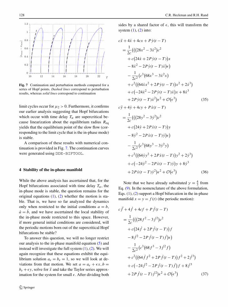
Fig. 7 Continuation and perturbation methods compared for aseries of Hopf points. Dashed lines correspond to perturbationresults, whereas solid lines correspond to continuation

limit cycles occur for μ2 > 0. Furthermore, it confirmsour earlier analysis suggesting that Hopf bifurcationswhich occur with time delay Tα are supercritical be-cause linearization about the equilibrium radius Req

yields that the equilibrium point of the slow flow (cor-responding to the limit cycle that is the in-phase mode)is stable.

A comparison of these results with numerical con-tinuation is provided in Fig. 7. The continuation curveswere generated using DDE-BIFTOOL.

4 Stability of the in-phase manifold

While the above analysis has ascertained that, for theHopf bifurcations associated with time delay Tα , thein-phase mode is stable, the question remains for theoriginal equations (1), (2) whether the motion is sta-ble. That is, we have so far analyzed the dynamicsonly when restricted to the initial conditions a = b,a = b, and we have ascertained the local stability ofthe in-phase mode restricted to this space. However,if more general initial conditions are considered, willthe periodic motions born out of the supercritical Hopfbifurcations be stable?

To answer this question, we will no longer restrictour analysis to the in-phase manifold equation (5) andinstead will investigate the full system (1), (2). We willagain recognize that these equations exhibit the equi-librium solution ae = be = 1, so we will look at de-viations from that motion. We set a = ae + εx, b =be + εy, solve for x and take the Taylor series approx-imation for the system for small ε. After dividing both

sides by a shared factor of ε, this will transform thesystem (1), (2) into:

cx + 4x + 4cx + P y(t − T )

= 1

2c

(((28x2 − 3x2)c2

+ c(24x + 2P y(t − T )

)x

− 8x2 − 2P y(t − T )x)ε)

− 1

2c2

(c3(68x3 − 3x2x

)+ c2((64xx2 + 2P y(t − T )

)x2 + 2x3)

+ c(−24x2 − 2P y(t − T )x

)x + 8x3

+ 2P y(t − T )x2)ε2 + O(ε3) (35)

cy + 4y + 4cy + P x(t − T )

= 1

2c

(((28y2 − 3y2)c2

+ c(24y + 2P x(t − T )

)y

− 8y2 − 2P x(t − T )y)ε)

− 1

2c2

(c3(68y3 − 3y2y

)

+ c2((64yy2 + 2P x(t − T ))y2 + 2y3)

+ c(−24y2 − 2P x(t − T )y

)y + 8y3

+ 2P x(t − T )y2)ε2 + O(ε3) (36)

Note that we have already substituted γ = 43 from

Eq. (9). In the nomenclature of the above formulation,Eqs. (1), (2) support a Hopf bifurcation in the in-phasemanifold x = y = f (t) (the periodic motion):

cf + 4f + 4cf + P f (t − T )

= 1

2c

(((28f 2 − 3f 2)c2

+ c(24f + 2P f (t − T )

)f

− 8f 2 − 2P f (t − T )f)ε)

− 1

2c2

(c3(68f 3 − 3f 2f

)

+ c2((64f f 2 + 2P f (t − T ))f 2 + 2f 3)

+ c(−24f 2 − 2P f (t − T )f

)f + 8f 3

+ 2P f (t − T )f 2)ε2 + O(ε3) (37)

Dynamics of microbubble oscillators with delay coupling 129

We have found the approximate solution of Eq. (37)for c = 94, P = 10, and T = Tcr + � to be

f (t) = Req cos((

ωcr + ε2k2)t)

(38)

where Req, k2 are calculated in the previous sectionfor delays Tcr corresponding to supercritical Hopfs;see Table 3. The goal is to determine the stability ofthe motion f (t) in Eq. (38). To do this, one may ana-lyze the linear variational equations of Eqs. (35), (36).Setting x = δx + f,y = δy + f and expanding forsmall δx, δy results in the linear variational equationsshown in Eqs. (39), (40). Note that here the notationxd = x(t − Tcr) and the same for y is used.

cδx + 4cδx + 4δx + Pδyd

= −1

c

((3f δx − 28f δx)c2

+ (−12f δx + (−P fd − 12f )δx − f Pδyd)c

+ (P fd + 8f )δx + P f δyd)ε

+ (((6f f δx + (

3f 2 − 204f 2)δx)c3

+ ((−6f 2 − 64f 2)δx− (4Pf fd + 128f f )δx − 2Pf 2δyd

)c2

+ ((2Pf fd + 48f f )δx

+ (2P fdf + 24f 2)δx + 2Pf f δyd

)c

− (4P fdf + 24f 2)δx

− 2P f 2δyd)ε2)/(2c2) + O

(ε3) (39)

cδy + 4cδy + 4δy + Pδxd

= −1

c

((3f δy − 28f δy)c2

+ (−12f δy + (−P fd − 12f )δy − f Pδxd)c

+ (P fd + 8f )δy + P f δxd)ε

+ (((6f f δy + (

3f 2 − 204f 2)δy)c3

+ ((−6f 2 − 64f 2)δy− (4Pf fd + 128f f )δy − 2Pf 2δxd

)c2

+ ((2Pf fd + 48f f )δy

+ (2P fdf + 24f 2)δy + 2Pf f δxd

)c

− (4P fdf + 24f 2)δy

− 2P f 2δxd)ε2)/(2c2) + O

(ε3) (40)

To analyze Eqs. (39), (40), we set u = δx − δy andv = δx +δy in order to transform the problem into “in-phase” and “out-of-phase” coordinates. We then addand subtract Eqs. (39), (40) to and from one anotherrespectively to obtain

cu + 4u + 4uc − P ud

= 1

c

((f − cf )P ud

+ (−fdP + (−3c2 − 8)f + 12cf

)u

+ (cfdP + 12cf + 28c2f

)u)ε

+ (((2f 2 − 2cf f + 2c2f 2)P ud

+ ((−4f + 2cf )fdP

+ (−6c2 − 24)f 2 + (

6c3 + 48c)f f − 64c2f 2)u

+ ((2cf − 4c2f

)fdP + (

3c3 + 24c)f 2

− 128c2f f − 204c3f 2)u)ε2)/(2c2) + O

(ε3)

(41)

cv + 4v + 4vc + P vd

= −1

c

((f − cf )P vd

+ (fdP + (

3c2 + 8)f − 12cf

)v

+ (−cfdP − 12cf − 28c2f)v)ε

− (((2f 2 − 2cf f + 2c2f 2)P vd

+ ((4f − 2cf )fdP + (

6c2 + 24)f 2

+ (−6c3 − 48c)f f + 64c2f 2)v

+ ((−2cf + 4c2f)fdP + (−3c3 − 24c

)f 2

+ 128c2f f + 204c3f 2)v)ε2)/(2c2) + O

(ε3)

(42)

Inspection shows that Eq. (42) is the variationalequation of Eq. (37). Because of this, it is seen thatv determines the stability of the motion x = y = f (t)

in the in-phase manifold, while u determines the sta-bility of the in-phase manifold. Since Eq. (42) is alinear delay-differential equation, its solution space isspanned by an infinite number of linearly independentsolutions. One of these solutions is v = df

dt, as may be

seen by differentiating Eq. (37) and comparing withEq. (42). The solution is periodic since f (t) is peri-odic. All other solutions of Eq. (42) are expected to be

130 C.R. Heckman and R.H. Rand

asymptotically stable for small ε, since as proven inthe previous section, f (t) is a limit cycle born in a su-percritical Hopf bifurcation. Therefore, the stability ofthe in-phase mode x = y = f (t) is determined solelyby Eq. (41).

It is notable that a basic difference between Eqs.(41) and (42) is that when ε = 0, Eq. (42) exhibits aperiodic solution (due to the Hopf bifurcation), whileEq. (41) does not. Thus, at ε = 0, Eq. (42) is struc-turally unstable, whereas Eq. (41) is structurally sta-ble. Therefore, for small values of ε, the stability ofEq. (41) is the same as it is for ε = 0. The stability ofEq. (41) (and of the in-phase mode x = y = f (t)) isthen determined by the behavior of the ε = 0 versionof Eq. (41):

cu + 4u + 4cu − P u(t − Tcr) = 0 (43)

To solve Eq. (43), set u = exp(λt) and obtain thecharacteristic equation

cλ2 + 4λ + 4cλ − P exp(−λTcr) = 0 (44)

Writing λ = a+ ib and equating imaginary and realparts yields:

0 =P exp(−aTcr) sin(bTcr) + 4b + 2abc (45)

0 =P exp(−aTcr) cos(bTcr) − 4a + c(b2 − a2 − 4

)(46)

For stability, all roots to Eqs. (45), (46) must havea < 0. For instability, there must be at least one rootfor which a > 0.

Figure 8 shows plots of the implicit functions inEqs. (45), (46), where intersections of the curves des-ignate solutions to the system of simultaneous equa-tions. Inspection shows that there are no roots forwhich a > 0, showing that the in-phase mode is sta-ble. These plots are only shown for the first few valuesof delay for which their is a supercritical Hopf bifur-cation.

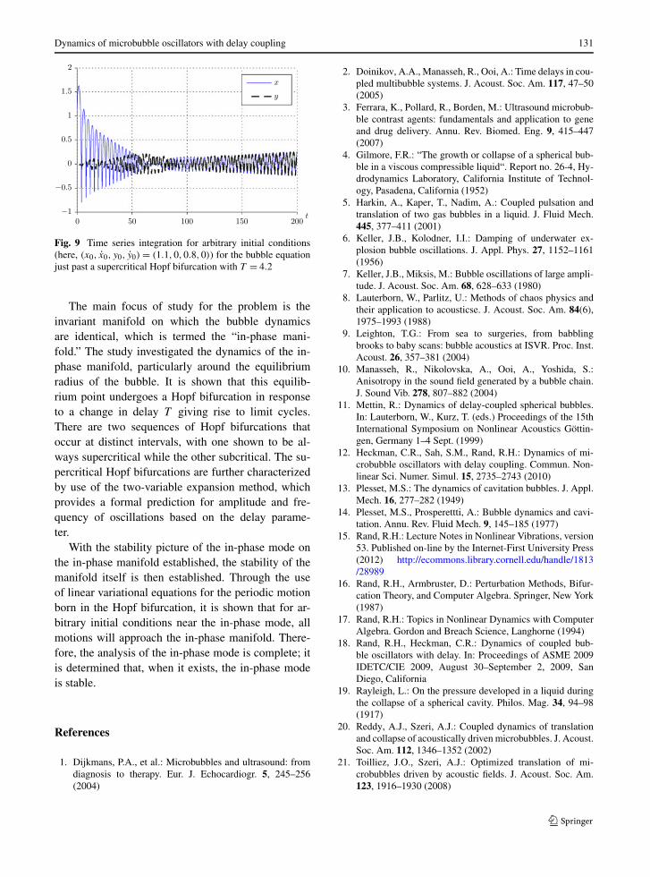
This conclusion is supported by numerical integra-tion using the MATLAB toolbox dde23, for which weshow a characteristic time integration in Fig. 9. Thetime integration features an arbitrary choice of initialconditions off the in-phase manifold, and it is wit-nessed that the solution approaches the in-phase mode.

5 Conclusion

This work has investigated the stability of periodicmotions that arise from a differential-delay equationassociated with the coupled dynamics of two oscillat-ing bubbles. The delayed dynamics arise as a resultof the finite speed of sound in the surrounding fluid,leading to a nonnegligible propagation time for wavescreated by one bubble to reach the other.

Fig. 8 Plot of the curves inEqs. (45), (46) for(i.) Tcr = 0.96734,(ii.) Tcr = 4.03324,(iii.) Tcr = 7.09919, and(iv.) Tcr = 10.165.Solid lines are plots of Eq.(45), dashed lines are plotsof Eq. (46)

Dynamics of microbubble oscillators with delay coupling 131

Fig. 9 Time series integration for arbitrary initial conditions(here, (x0, x0, y0, y0) = (1.1,0,0.8,0)) for the bubble equationjust past a supercritical Hopf bifurcation with T = 4.2

The main focus of study for the problem is theinvariant manifold on which the bubble dynamicsare identical, which is termed the “in-phase mani-fold.” The study investigated the dynamics of the in-phase manifold, particularly around the equilibriumradius of the bubble. It is shown that this equilib-rium point undergoes a Hopf bifurcation in responseto a change in delay T giving rise to limit cycles.There are two sequences of Hopf bifurcations thatoccur at distinct intervals, with one shown to be al-ways supercritical while the other subcritical. The su-percritical Hopf bifurcations are further characterizedby use of the two-variable expansion method, whichprovides a formal prediction for amplitude and fre-quency of oscillations based on the delay parame-ter.

With the stability picture of the in-phase mode onthe in-phase manifold established, the stability of themanifold itself is then established. Through the useof linear variational equations for the periodic motionborn in the Hopf bifurcation, it is shown that for ar-bitrary initial conditions near the in-phase mode, allmotions will approach the in-phase manifold. There-fore, the analysis of the in-phase mode is complete; itis determined that, when it exists, the in-phase modeis stable.

References

1. Dijkmans, P.A., et al.: Microbubbles and ultrasound: fromdiagnosis to therapy. Eur. J. Echocardiogr. 5, 245–256(2004)

2. Doinikov, A.A., Manasseh, R., Ooi, A.: Time delays in cou-pled multibubble systems. J. Acoust. Soc. Am. 117, 47–50(2005)

3. Ferrara, K., Pollard, R., Borden, M.: Ultrasound microbub-ble contrast agents: fundamentals and application to geneand drug delivery. Annu. Rev. Biomed. Eng. 9, 415–447(2007)

4. Gilmore, F.R.: “The growth or collapse of a spherical bub-ble in a viscous compressible liquid“. Report no. 26-4, Hy-drodynamics Laboratory, California Institute of Technol-ogy, Pasadena, California (1952)

5. Harkin, A., Kaper, T., Nadim, A.: Coupled pulsation andtranslation of two gas bubbles in a liquid. J. Fluid Mech.445, 377–411 (2001)

6. Keller, J.B., Kolodner, I.I.: Damping of underwater ex-plosion bubble oscillations. J. Appl. Phys. 27, 1152–1161(1956)

7. Keller, J.B., Miksis, M.: Bubble oscillations of large ampli-tude. J. Acoust. Soc. Am. 68, 628–633 (1980)

8. Lauterborn, W., Parlitz, U.: Methods of chaos physics andtheir application to acousticse. J. Acoust. Soc. Am. 84(6),1975–1993 (1988)

9. Leighton, T.G.: From sea to surgeries, from babblingbrooks to baby scans: bubble acoustics at ISVR. Proc. Inst.Acoust. 26, 357–381 (2004)

10. Manasseh, R., Nikolovska, A., Ooi, A., Yoshida, S.:Anisotropy in the sound field generated by a bubble chain.J. Sound Vib. 278, 807–882 (2004)

11. Mettin, R.: Dynamics of delay-coupled spherical bubbles.In: Lauterborn, W., Kurz, T. (eds.) Proceedings of the 15thInternational Symposium on Nonlinear Acoustics Göttin-gen, Germany 1–4 Sept. (1999)

12. Heckman, C.R., Sah, S.M., Rand, R.H.: Dynamics of mi-crobubble oscillators with delay coupling. Commun. Non-linear Sci. Numer. Simul. 15, 2735–2743 (2010)

13. Plesset, M.S.: The dynamics of cavitation bubbles. J. Appl.Mech. 16, 277–282 (1949)

14. Plesset, M.S., Prosperettti, A.: Bubble dynamics and cavi-tation. Annu. Rev. Fluid Mech. 9, 145–185 (1977)

15. Rand, R.H.: Lecture Notes in Nonlinear Vibrations, version53. Published on-line by the Internet-First University Press(2012) http://ecommons.library.cornell.edu/handle/1813/28989

16. Rand, R.H., Armbruster, D.: Perturbation Methods, Bifur-cation Theory, and Computer Algebra. Springer, New York(1987)

17. Rand, R.H.: Topics in Nonlinear Dynamics with ComputerAlgebra. Gordon and Breach Science, Langhorne (1994)

18. Rand, R.H., Heckman, C.R.: Dynamics of coupled bub-ble oscillators with delay. In: Proceedings of ASME 2009IDETC/CIE 2009, August 30–September 2, 2009, SanDiego, California

19. Rayleigh, L.: On the pressure developed in a liquid duringthe collapse of a spherical cavity. Philos. Mag. 34, 94–98(1917)

20. Reddy, A.J., Szeri, A.J.: Coupled dynamics of translationand collapse of acoustically driven microbubbles. J. Acoust.Soc. Am. 112, 1346–1352 (2002)

21. Toilliez, J.O., Szeri, A.J.: Optimized translation of mi-crobubbles driven by acoustic fields. J. Acoust. Soc. Am.123, 1916–1930 (2008)

132 C.R. Heckman and R.H. Rand

22. Wirkus, S., Rand, R.: Dynamics of two coupled Van DerPol oscillators with delay coupling. Nonlinear Dyn. 30,205–221 (2002)

23. Yamakoshi, Y., Ozawa, Y., Ida, M., Masuda, N.: Effects ofBjerknes forces on Gas-Filled microbubble trapping by ul-trasonic waves. Jpn. J. Appl. Phys. 40, 3852–3855 (2001)

24. Heckman, C.R., Rand, R.H.: Asymptotic analysis of theHopf-Hopf bifurcation in a time-delay system. J. Appl.Nonlinear Dyn. 1(2), 159–171 (2012)

25. Suchorsky, M.K., Sah, S.M., Rand, R.H.: Using delay toquench undesirable vibrations. Nonlinear Dyn. 62, 107–116 (2010)

26. Heckman, C.R., Rand, R.H.: Dynamics of coupled mi-crobubbles with large fluid compressibility delays. In: Proc.EUROMECH 2011 Euro. Nonlin. Osc. Conf

27. Rand, R.H.: Differential-Delay equations. In: Luo, A.C.J.,Sun, J.-Q. (eds.) Complex Systems: Fractionality, Time-delay and Synchronization, pp. 83–117. Springer, Berlin(2011)

28. Engelborghs, K., Luzyanina, T., Samaey, G., Roose, D.,Verheyden, K.: DDE-BIFTOOL. Available from http://twr.cs.kuleuven.be/research/software/delay/ddebiftool.shtml