dynamics of molecular motors in reversible burnt-bridge...

Condensed Matter Physics 2010, Vol. 13, No 2, 23801: 1–18

http://www.icmp.lviv.ua/journal

Dynamics of molecular motors in reversibleburnt-bridge models

M.N. Artyomov1, A.Yu. Morozov2, A.B. Kolomeisky3

1 Department of Chemistry, Massachusetts Institute of Technology, Cambridge, MA 02139, USA2 Department of Physics and Astronomy, University of California, Los Angeles, Los Angeles, CA 90095, USA3 Department of Chemistry, Rice University, Houston, TX 77005, USA

Received November 23, 2009

Dynamic properties of molecular motors whose motion is powered by interactions with specific lattice bondsare studied theoretically with the help of discrete-state stochastic “burnt-bridge” models. Molecular motors aredepicted as random walkers that can destroy or rebuild periodically distributed weak connections (“bridges”)when crossing them, with probabilities p1 and p2 correspondingly. Dynamic properties, such as velocitiesand dispersions, are obtained in exact and explicit form for arbitrary values of parameters p1 and p2. For theunbiased random walker, reversible burning of the bridges results in a biased directed motion with a dynamictransition observed at very small concentrations of bridges. In the case of backward biased molecular motorits backward velocity is reduced and a reversal of the direction of motion is observed for some range ofparameters. It is also found that the dispersion demonstrates a complex, non-monotonic behavior with largefluctuations for some set of parameters. Complex dynamics of the system is discussed by analyzing thebehavior of the molecular motors near burned bridges.

Key words: molecular motors, stochastic models, motor proteins

PACS: 87.16.Ac

1. Introduction

In recent years an increased attention has been devoted to investigations of molecular motors,also known as motor proteins, that are crucial in many cellular processes [1]. They transformchemical energy into the mechanical motion in non-equilibrium conditions. For most of molecularmotors their motion along linear molecular tracks is fueled by the hydrolysis of adenosine tri-phosphate (ATP) or related compounds. It was suggested that a different mechanism is employedto power the motion of a protein collagenase along collagen fibrils [2, 3]. It probably utilizes thecollagen proteolysis, cleaving the filament at specific sites. As the collagenase molecule is unableto cross the already broken bond, it leads to the biased diffusion along the filament. However, fullunderstanding of mechanisms of collagenase motion is still not available.

It was proposed that a good description of the collagenase dynamics could be provided bythe so-called “burnt-bridge model” (BBM) [2–9]. In this model, the motor protein is depicted asa random walker that translocates along the one-dimensional lattice that consists of strong andweak bonds. While the strong bonds remain unaffected if crossed by the walker in any direction,the weak ones (termed “bridges”) might be broken (or “burnt”) with a probability 0 < p1 6 1when crossed in the specific direction, and the walker cannot cross the burnt bridges again, unlessthey are restored, which can occur with probability 0 < p2 6 1. In [6, 7] an analytical approachwas developed which permitted us to derive the explicit formulas for molecular motor velocityV (c, p1) and diffusion constant D(c, p1) for the entire ranges of burning probability 0 < p1 6 1and concentration of the bridges 0 < c 6 1 which were also confirmed by extensive Monte Carlocomputer simulations. This theoretical method has been applied to several problems with periodicbridge distribution. However, the results in [6, 7] have been obtained only for irreversible bridgeburning (bridge recovery probability was taken to be p2 = 0), and also for unbiased random walkerbetween bridges (equal forward and backward transition rates). In present work, we generalize

c© M.N. Artyomov, A.Yu. Morozov, A.B. Kolomeisky 23801-1

http://www.icmp.lviv.ua/journal

M.N. Artyomov, A.Yu. Morozov, A.B. Kolomeisky

our approach to allow for the possibility of bridge recovery as well as unequal hopping rates onthe sites between bridges. It is more realistic to consider systems with reversible action of motorproteins since they are catalysts that equally accelerate both forward and backward biochemicaltransitions [1].

2. Model

According to our model, we view a motor protein as a random walker moving along an infiniteone-dimensional lattice with forward and backward transition rates being u and w correspondingly,as illustrated in figure 1. The lattice spacing size is set to be equal to one. The lattice is composedof strong and weak bonds. There is no interaction between the random walker and strong bonds.However, crossing the bridge in the forward direction (from left to right) leads to its burning withthe probability p1, while the particle moves with the rate u. After the weak link is destroyed, thewalker is assumed to be on the right side of it. When the particle is trying to cross a broken bond,the bridge can be recovered with the probability p2, while the particle moves to the left with ratew. It is assumed that initially, at t = 0, all bridges are intact.

p1

p2

w u

−1 0 1 2 N−1 N

Figure 1. A schematic picture of the motion of a molecular motor in the reversible burnt-bridge model. Thick solid lines depict strong links, while thin solid lines represent periodicallydistributed weak links (bridges). Dotted lines are for already burnt bridges.

The details of breaking weak bonds in BBM have a strong effect on the dynamic propertiesof motor proteins [6]. There are two different possibilities of bridge burning. In the first variant(the so-called “forward BBM”), the weak bond is broken when crossed from left to right, but theintact bridge is not affected when the particle moves from right to left. Thus the bridge recoverymay occur if the walker attempts to cross a burnt bridge from right to left. In the second variant(named “forward-backward BBM”), the weak link is destroyed if crossed in either direction [4, 5].Both variants are identical for p1 = 1, however for p1 < 1 the dynamics is different in two burningscenarios, as was shown in p2 = 0 case [6], although mechanisms are still the same. For reasonsof simplicity, below we will only consider forward BBM, even though forward-backward BBM canalso be solved using the same method.

There are five parameters that specify the dynamics of molecular motors in BBM: the prob-abilities p1, p2, the concentration of bridges c, as well as transition rates u and w. The dynamicproperties of the walker are also strongly effected by the distribution of weak bonds [5]. Below wewill study the case of periodically distributed bridges, when their concentration is c = 1/N and theweak bonds are located between the lattice sites with the coordinates kN −1 and kN , with integerk (see figure 1). This description is more realistic for collagenases’ dynamics [2, 3]. The modelbelow will be studied using continuous time analysis as it better describes chemical transitions inmotor proteins [6].

3. Dynamic properties for BBM with bridge recovery

3.1. Velocity

To find the walker’s velocity, we generalize the method used in [6] (for irreversible bridgeburning, i.e. p2 = 0) to allow for non-zero probability p2. We introduce a probability Rj(t) thatthe random walker is found j sites apart from the last burnt bridge at time t. The probabilitiesRj(t) arise if the system is viewed in moving coordinate frame with the last burnt bridge alwaysat the origin, as illustrated by a reduced chemical kinetic scheme shown in figure 2.

23801-2

Reversible burnt-bridge models

1

p2 f(1)

2

2

p

p

p

0 1 2 NN−1

1−p 1−p

2N

p f(2)

p f(3)

1 1

1

1

Figure 2. Reduced kinetic scheme for continuous-time forward BBM with bridge recovery (onlytransition rates not equal to u, w are shown). The origin is the right end of the last burnt bridge.Parameters are described in detail in the text.

The dynamics of the system is determined by a set of master equations:

dRkN+i(t)

dt= uRkN+i−1(t) + wRkN+i+1(t) − (u + w)RkN+i(t), (1)

for k = 0, 1, 2, · · · and i = 1, 2, · · · , N − 2; and

dRkN+N−1(t)

dt= uRkN+N−2(t) + wp2f(k + 1)R0(t) + wR(k+1)N (t) − (u + w)RkN+N−1(t), (2)

dR(k+1)N (t)

dt= (1 − p1)uRkN+N−1(t) + wR(k+1)N+1(t) − (u + w)R(k+1)N (t), (3)

with k = 0, 1, 2, · · · for both equations (2) and (3). Also at the origin we have

dR0(t)

dt= p1u

∞∑

k=1

[RkN−1(t)] + wR1(t) − uR0(t) − wp2R0(t). (4)

In equation (2) we introduced a function f(k) as a probability that next to the last burnt bridge

is k periods to the left from the last burnt bridge. It satisfies the condition∞∑

k=1

f(k) = 1, which is

reflected in equation (4). The system of equations (1)–(4) is to be solved in the stationary-statelimit (at large times) when dRj(t)/dt = 0 is satisfied, and we denote Rj(t → ∞) ≡ Rj in whatfollows. By definition, it can be argued that

f(k) =p1RkN−1

∞∑

k=1

p1RkN−1

. (5)

The solution of the system (1)–(4) can be facilitated by rewriting equation (5) in a more convenientform. To this end, we note that based on the results from [6, 8] it is reasonable to assume thatRkN+i is of the form

RkN+i = ykW (i), (6)

where y and W are some functions of p1, p2, u, w and N . Furthermore, y is i and k-independent,while W depends on i (but not on k). The advantage of the ansatz (6) is that it leads to a simplerform of f(k):

f(k) = yk−1(1 − y), (7)

as follows from equation (5). We proceed to solve equations (1)–(4) with f(k) in equation (2) givenby the expression (7).

23801-3


Introducing a parameter β ≡ u/w, it can be easily verified that

RkN+i = C1(k) + C2(k)βi (8)

with arbitrary C1(k), C2(k) solves equation (1). Utilizing equation (8), C1(k), C2(k) can be ex-pressed in terms of functions RkN and RkN+1 (first two points of the period). Then equation (8)leads to

RkN+i = RkN − w

u − w

[

1 − βi]

∆k , (9)

where we defined∆k = RkN+1 − RkN . (10)

In expression (9) it was assumed that k = 0, 1, 2, · · · and i = 0, 1, · · · , N − 1. Parameters RkN

and ∆k are to be determined from equations (2) and (3). Substituting equation (9) in (2) and (3)yields

uRkN − uw

u − w

[

1 − βN−2]

∆k + wp2yk(1 − y)R0 + wR(k+1)N − (u + w)RkN

+ (u + w)w

u − w

[

1 − βN−1]

∆k = 0, (11)

(1 − p1)uRkN − (1 − p1)uw

u − w

[

1− βN−1]

∆k + wR(k+1)N

− w2

u − w[1 − β] ∆k+1 − (u + w)R(k+1)N = 0. (12)

Equation (11) also yields

∆k =u − w

w(1 − βN )

[

RkN − R(k+1)N − p2yk(1 − y)R0

]

. (13)

Substituting (13) into equation (12) results in

aRkN + bR(k+1)N + cR(k+2)N + (d + ey + fy2)R0yk = 0, (14)

where

a = (1 − p1)u

[

1 − 1 − βN−1

1 − βN

]

, (15)

b = −u + (1 − p1)u1 − βN−1

1 − βN− w

1 − β

1 − βN, (16)

c = w1 − β

1 − βN, (17)

d = p2(1 − p1)u1 − βN−1

1 − βN, (18)

e = −p2(1 − p1)u1 − βN−1

1 − βN+ wp2

1 − β

1 − βN, (19)

and

f = −wp21− β

1 − βN. (20)

Using equation (6), it follows thatRkN = R0y

k, (21)

and equation (14) turns into

(c + f)y2 + (b + e)y + (a + d) = 0. (22)

23801-4


Therefore,

y =−(b + e) −

√

(b + e)2 − 4(a + d)(c + f)

2(c + f), (23)

where we selected the solution of (22) such that 0 6 y < 1. With the help of (21) we obtain fromequation (13)

∆k =u − w

w {1 − βN}R0yk(1 − y)(1 − p2). (24)

Thus (9) yields

RkN+i = R0yk

[

1 − (1 − p2)(1 − y)1 − βi

1 − βN

]

. (25)

Equation (25) with y given by (23) solves the system of equations (1)–(4) in the stationary statelimit. We note that although the equation (4) was not used to find this solution, it was numericallyverified that every equation in the system (1)–(4) is indeed solved by expressions (25) and (23).

Parameter R0, needed to find the velocity, is found from equation (25) combined with the

normalization condition∞∑

k=0

N−1∑

i=0

RkN+i = 1, which produces

R0 = (1 − y)

{

N − (1 − p2)(1 − y)

[

N

1 − βN− 1

1 − β

]}−1

. (26)

The mean velocity of the walker is given by [6]

V =

∞∑

j=0

(uj − wj)Rj = (u − wp2)R0 +

[

∞∑

k=0

N−1∑

i=0

(u − w)RkN+i

]

− (u − w)R0 , (27)

which results in a simple relation,

V = w(1 − p2)R0 + (u − w). (28)

In equation (28), R0 is given by (26) with y from the expression (23).It can be shown that in the limit of u → 1, w → 1, and p2 → 0 equation (28) reproduces

the result obtained earlier in [6] for the BBM with u = w = 1 and p2 = 0. Also, equation (28)considerably simplifies in the limiting case of p1 = 1 (deterministic bridge burning) when y = 0.In the case of p1 = 1 we obtained V (u, w, p2, N) in [9] using the Derrida’s method [10] and ourgeneral result given in equation (28) agrees with it in the p1 → 1 limit, as was numerically verified.

3.2. Diffusion coefficient

The diffusion coefficient is found by generalizing the method developed in [7] (where we founddynamic properties of the random walker in BBM with u = w = 1, p2 = 0 and periodic bridgedistribution), allowing for 0 < p2 6 1 and u 6= w. We define PkN+i,m(t) as the probability that attime t the random walker is located at point x = kN + i (i = 0, 1, · · · , N − 1), the right end of thelast burnt bridge being at the point mN . Parameters m and k > 0 assume integer values.

The dynamics of the system is described by a set of Master equations:

dPmN,m(t)

dt= wPmN+1,m(t) − (u + p2w)PmN,m(t) + p1u

m−1∑

m′=−∞

PmN−1,m′(t), (29)

for k = i = 0,

dPmN+kN+(N−1),m(t)

dt= wPmN+(k+1)N,m(t) + uPmN+kN+(N−2),m(t)

+ p2wf(k + 1)PmN+(k+1)N,m+k+1(t) − (u + w)PmN+kN+(N−1),m(t), (30)

23801-5


for k > 0 and i = N − 1 [with f(k + 1) the same as in (2)],

dPmN+kN,m(t)

dt= wPmN+kN+1,m(t) + (1 − p1)uPmN+kN−1,m(t) − (u + w)PmN+kN,m(t) (31)

for k > 1 and i = 0, and

dPmN+kN+i,m(t)

dt= wPmN+kN+i+1,m(t) + uPmN+kN+i−1,m(t) − (u + w)PmN+kN+i,m(t) (32)

for k > 0 and i = 1, · · · , N − 2.We observe that

RkN+i(t) =+∞∑

m=−∞

P(m+k)N+i,m(t), (k > 0; i = 0, 1, · · · , N − 1), (33)

where RkN+i(t) is the probability for the random walker to be found kN + i sites apart from thelast burnt bridge at time t, which was used above to find the walker’s velocity and is given byequation (25). Plugging (33) into equations (29)–(32) results in the equations (1)–(4) for RkN+i,thus obtained by a different method.

In accordance with [7, 10], we introduce auxiliary functions SkN+i(t),

SkN+i(t) =

+∞∑

m=−∞

(mN + kN + i)PmN+kN+i,m(t), (k > 0 i = 0, 1, · · · , N − 1). (34)

The system of equations describing the time evolution of the functions SkN+i(t) results fromequations (34) and (29)–(32). It was obtained that

dS0(t)

dt= wS1(t) − (u + p2w)S0(t) + p1u

∞∑

α=1

SαN−1(t) + p1u∞∑

α=1

RαN−1(t) − wR1(t), (35)

dSkN+(N−1)(t)

dt= wS(k+1)N (t) + uSkN+(N−2)(t) + p2wf(k + 1)[S0 − R0]

− (u + w)SkN+(N−1)(t) − wR(k+1)N (t) + uRkN+(N−2)(t), (36)

for k > 0,

dSkN (t)

dt= wSkN+1(t)+(1−p1)uSkN−1(t)−(u+w)SkN (t)+(1−p1)uRkN−1(t)−wRkN+1(t) (37)

for k > 1 and

dSkN+i(t)

dt= wSkN+i+1(t) +uSkN+i−1(t)− (u + w)SkN+i(t) +uRkN+i−1(t)−wRkN+i+1(t) (38)

for k > 0 and i = 1, · · · , N − 2.At t → ∞ the solutions of equations (35)–(38) are sought in the form

Sj(t) = ajt + Tj , (39)

where aj and Tj are time-independent coefficients. Plugging equation (39) into equations (35)–(38)leads to,

wa1 − (u + p2w)a0 + p1u

∞∑

α=1

aαN−1 = 0, (40)

wa(k+1)N + uakN+(N−2) + p2wf(k + 1)a0 − (u + w)akN+(N−1) = 0 (41)

23801-6


for k > 0,wakN+1 + (1 − p1)uakN−1 − (u + w)akN = 0 (42)

for k > 1 andwakN+i+1 + uakN+i−1 − (u + w)akN+i = 0 (43)

for k > 0 and i = 1, · · · , N − 2.Clearly, equations (40)–(43) are identical to the system of equations (1)–(4) for the functions Rj

in the t → ∞ limit, where dRj/dt = 0. Thus their solutions should coincide up to the multiplicativeconstant, namely,

akN+i = CRkN+i , (44)

with RkN+i given by equation (25). The normalization condition∞∑

k=0

N−1∑

i=0

RkN+i = 1 implies that

C =∞∑

k=0

N−1∑

i=0

akN+i. To find the explicit expression for C, we utilize the equations for Tj obtained

by plugging equation (39) into equations (35)–(38),

a0 = wT1 − (u + p2w)T0 + p1u

∞∑

α=1

TαN−1 + p1u

∞∑

α=1

RαN−1 − wR1 , (45)

akN+(N−1) = wT(k+1)N + uTkN+(N−2) + p2wf(k + 1)[T0 − R0] − (u + w)TkN+(N−1)

+ uRkN+(N−2) − wR(k+1)N (46)

for k > 0,

akN = wTkN+1 + (1 − p1)uTkN−1 − (u + w)TkN + (1 − p1)uRkN−1 − wRkN+1, (47)

for k > 1 and

akN+i = wTkN+i+1 + uTkN+i−1 − (u + w)TkN+i + uRkN+i−1 − wRkN+i+1, (48)

for k > 0 and i = 1, · · · , N −2. Summing up equations (45)–(48) and using∞∑

k=0

f(k +1) = 1 yields

C =

∞∑

k=0

N−1∑

i=0

akN+i = w(1 − p2)R0 + (u − w) = V, (49)

where the walker’s velocity V is given by (28). Hence, in accordance with equation (44)

akN+i = V RkN+i (50)

where RkN+i and V are given by equations (25) and (28).Now we are able to obtain the expression for the random walker’s velocity [7]. The mean position

of the particle is given by

〈x(t)〉 =

+∞∑

m=−∞

∞∑

k=0

N−1∑

i=0

(mN + kN + i)PmN+kN+i,m(t)

=∞∑

k=0

N−1∑

i=0

{

+∞∑

m=−∞

(mN + kN + i)PmN+kN+i,m(t)

}

=∞∑

k=0

N−1∑

i=0

SkN+i(t), (51)

which results in the mean velocity

V =d

dt〈x(t)〉 =

∞∑

k=0

N−1∑

i=0

d

dtSkN+i(t). (52)

23801-7


In the t → ∞ limit equations (39) and (49) therefore yield

V =∞∑

k=0

N−1∑

i=0

akN+i = w(1 − p2)R0 + (u − w) = V. (53)

As expected, equation (53) reproduces the expression (28) for V obtained above with the use ofthe reduced chemical kinetic scheme method.

For the purposes of computing the diffusion coefficient D, functions TkN+i need to be foundfrom (45)–(48) [7, 10]. In (45)–(48), akN+i should be expressed according to (50). In analogy withfinding RkN+i from (1)–(4), we start with solving (48). In the expression (25) for RkN+i, we denote

ξ =(1 − p2)(1 − y)

1− βN, (54)

so thatRkN+i = RkN [1 − ξ(1 − βi)], (55)

where RkN = R0yk, with R0, y given by (26), (23). With the use of (55), (48) takes the form

wTkN+i+1 + uTkN+i−1 − (u + w)TkN+i + (u−w− V )RkN (1− ξ) + (w −u−V )RkN ξβi = 0. (56)

We seek the solution of (56) in the form

TkN+i = C1(k) + C2(k)βi + iA(k) + iB(k)βi. (57)

In (57), C1(k) + C2(k)βi part is the solution of homogeneous equation [the part of (56) whichinvolves only TkN+i, TkN+i±1], in analogy with equation (8). Substituting equation (57) into equa-tion (56) gives these expressions for A(k) and B(k):

A(k) =u − w − V

u − wRkN (1 − ξ), B(k) =

u − w + V

u − wRkNξ. (58)

Plugging TkN , TkN+1 instead of TkN+i into (57), one can express C1(k) and C2(k) in terms ofA(k), B(k) as well as TkN and TkN+1 (first two points of the period). Substituting the resultingexpressions for C1(k) and C2(k) together with the expressions (58) for A(k), B(k) in (57) givesafter some rearrangement

TkN+i = TkN + θk

1 − βi

1 − β+ RkN

u − w − V

u − w(1 − ξ)

[

i − 1 − βi

1 − β

]

+ RkN

u − w + V

u − wξ

[

iβi − β1 − βi

1 − β

]

, (59)

whereθk = TkN+1 − TkN . (60)

Equation (59) solves (56) [i.e., the equation (48)] for arbitrary TkN and θk. Parameters TkN andθk are to be determined from the equations (46) and (47). To get a less cumbersome result forTkN+i, it is convenient to rewrite equation (46) by adding and subtracting wTkN+N , wRkN+N

[we note that TkN+N , RkN+N are given by (59) and (55) with i = N , i.e., TkN+N 6= T(k+1)N ,RkN+N 6= R(k+1)N ]:

akN+(N−1) = wT(k+1)N − wTkN+N + wTkN+N + uTkN+(N−2) + p2wf(k + 1)[T0 − R0]

− (u + w)TkN+(N−1) + uRkN+(N−2) − wRkN+N + w(RkN+N − R(k+1)N ), (61)

which gives

w(T(k+1)N − TkN+N ) + w(RkN+N − R(k+1)N ) + p2wf(k + 1)[T0 − R0] = 0, (62)

23801-8


as follows from (48) which was formally extended to include i = N − 1. In (62), the functionf(k + 1) is expressed according to equation (7). Plugging (59), (55) (with appropriate k, i) into(62) permits us to express θk in terms of TkN in this way,

θk =1 − β

1 − βN

{

T(k+1)N − TkN − FRkN + p2yk(1 − y)T0

}

, (63)

where

F =u − w − V

u − w(1 − ξ)

[

N − 1 − βN

1 − β

]

+u − w + V

u − wξ

[

NβN − β1 − βN

1− β

]

. (64)

It should be mentioned that substituting (59) and (55) into original equation (46) leads to a moreinvolved expression connecting θk and TkN which turns out to be identical to equation (63), as wasnumerically verified.

To find TkN , we substitute (59) and (55) (with appropriate k, i) in equation (47), with θk in(59) replaced according to (63). After some algebra, this results in

aTkN + bT(k+1)N + cT(k+2)N + {d + ey + fy2}T0yk + χyk = 0, (65)

where coefficients a, b, c, d, e, f are given by equations (15)–(20) and

χ = −R0F

[

wy1 − β

1 − βN+ (1 − p1)u

1 − βN−1

1 − βN

]

+ R0

{

(1 − p1)uφ − wy[1 − ξ(1 − β)]

+(1− p1)u[1 − ξ(1 − βN−1)] − V y}

. (66)

In equation (66) it was found that

φ =u − w − V

u − w(1 − ξ)

[

N − 1 − 1 − βN−1

1 − β

]

+u − w + V

u − wξ

[

(N − 1)βN−1 − β1 − βN−1

1 − β

]

(67)

and F is given by (64).Comparison between (65) and (14) shows that they are identical (with replacement R → T ),

with the exception of χyk term in (65). This implies that

T(1)kN = Byk (68)

with arbitrary constant B solves homogeneous equation [equation (65) without χyk term], since ygiven by (23) is constructed for RkN = R0y

k to solve specifically equation (14).To account for χyk term, we look for solution of (65) of the form

T(2)kN = Czk, (69)

where

z =−b−

√b2 − 4ac

2c(70)

with a, b, c given by (15)–(17); parameter C is to be determined. Parameter z is the solution ofequation cz2 + bz + a = 0 such that 0 6 z < 1. Plugging (69) into (65) gives

Czk(a + bz + cz2) + (d + ey + fy2)Cyk + χyk = 0. (71)

The first term in (71) vanishes since z is given by (70), thus (71) yields

C =−χ

d + ey + fy2. (72)

The T(2)kN given by (69) with C specified by (72) therefore solves equation (65). More generally, (65)

is solved by the sum of contributions (68) and (69), i. e.

TkN = Byk + Czk, (73)

23801-9


where B remains undetermined. Plugging (73) in equation (63) for θk gives

θk =1 − β

1 − βN

{

Byk(y − 1) + Czk(z − 1) − FR0yk + p2y

k(1 − y)[B + C ]}

. (74)

Substituting (73) and (74) into (59) results in the final expression for TkN+i,

TkN+i = Byk + Czk +1 − βi

1 − βN

{

Byk(y − 1) + Czk(z − 1) − FR0yk + p2y

k(1 − y)[B + C]}

+ R0yk

{

u − w − V

u − w(1 − ξ)

[

i − 1 − βi

1 − β

]

+u − w + V

u − wξ

[

iβi − β1 − βi

1 − β

]}

. (75)

Although equation (45) was not utilized to obtain (75), it was numerically checked that everyequation in the system (45)–(48) holds for TkN+i, RkN+i given by (75) and (25).

To compute the diffusion coefficient D, we need to consider additional auxiliary functions [7, 10],

UkN+i(t) =

+∞∑

m=−∞

(mN + kN + i)2PmN+kN+i,m(t), k > 0, i = 0, 1, · · · , N − 1. (76)

A system of equations which determine the time evolution of Uj(t) is derived with the use ofequations (76), (34) and (33) for UkN+i(t), SkN+i(t) and RkN+i(t), as well as equations (29)–(32).It follows that

dU0(t)

dt= wU1(t) − (u + p2w)U0(t) − 2wS1(t) + wR1(t) + p1u

∞∑

α=1

UαN−1(t)

+ 2p1u

∞∑

α=1

SαN−1(t) + p1u

∞∑

α=1

RαN−1(t), (77)

dUkN+(N−1)(t)

dt= wU(k+1)N (t) + uUkN+(N−2)(t) − (u + w)UkN+(N−1)(t)

+ p2wf(k + 1)U0(t) − 2wS(k+1)N (t) + 2uSkN+(N−2)(t)

− 2p2wf(k + 1)S0(t) + wR(k+1)N (t) + uRkN+(N−2)(t)

+ p2wf(k + 1)R0(t) (78)

for k > 0,

dUkN (t)

dt= wUkN+1(t) + (1 − p1)uUkN−1(t) − (u + w)UkN (t) − 2wSkN+1(t)

+ 2(1− p1)uSkN−1(t) + wRkN+1(t) + (1 − p1)uRkN−1(t) (79)

for k > 1, and

dUkN+i(t)

dt= wUkN+i+1(t) + uUkN+i−1(t) − (u + w)UkN+i(t) − 2wSkN+i+1(t)

+ 2uSkN+i−1(t) + wRkN+i+1(t) + uRkN+i−1(t) (80)

for k > 0 and i = 1, · · · , N − 2.

The diffusion constant is to be found from

D =1

2lim

t→∞

d

dt

[

〈x(t)2〉 − 〈x(t)〉2]

. (81)

23801-10


Using (76) and summing up equations (77)–(80) results in

d

dt〈x(t)2〉 =

d

dt

+∞∑

m=−∞

∞∑

k=0

N−1∑

i=0

(mN + kN + i)2PmN+kN+i,m(t)

=d

dt

∞∑

k=0

N−1∑

i=0

UkN+i(t) =∞∑

k=0

N−1∑

i=0

dUkN+i(t)

dt

= (u + w) − w(1 − p2)R0(t) + 2w(1 − p2)S0(t) + 2(u − w)

∞∑

k=0

N−1∑

i=0

SkN+i(t), (82)

thus we do not need to find UkN+i(t) from the system (77)–(80) to obtain the diffusion coefficient.

To derive (82) we used the normalization conditions,∞∑

k=0

N−1∑

i=0

RkN+i(t) = 1 and∞∑

k=0

f(k + 1) = 1.

In the t → ∞ limit, SkN+i(t) → akN+it + TkN+i, R0(t) → R0, thus (82) becomes

d

dt〈x(t)2〉 = (u+w)−w(1−p2)R0 +2w(1−p2)[a0t+T0]+2(u−w)

∞∑

k=0

N−1∑

i=0

[akN+it+TkN+i]. (83)

Given that in the stationary-state limit ddt〈x(t)〉 =

∞∑

k=0

N−1∑

i=0

akN+i = w(1 − p2)R0 + (u − w) = V

[equation (53)] and utilizing 〈x(t)〉 given by (51), it follows that

d

dt〈x(t)〉2 = 2〈x(t)〉 d

dt〈x(t)〉 = 2V 〈x(t)〉 = 2V

∞∑

k=0

N−1∑

i=0

SkN+i(t → ∞)

= 2[w(1 − p2)R0 + (u − w)]

∞∑

k=0

N−1∑

i=0

{akN+it + TkN+i} . (84)

Plugging (83) and (84) into (81) gives the diffusion constant,

D=1

2

[

(u + w) − w(1 − p2)R0 + 2w(1 − p2)[a0t + T0] − 2w(1 − p2)R0

∞∑

k=0

N−1∑

i=0

{akN+it + TkN+i}]

.

(85)The time-dependent part of (85) is

D(t) =1

2

[

2w(1 − p2)a0t − 2w(1 − p2)R0

∞∑

k=0

N−1∑

i=0

akN+it

]

. (86)

Using∞∑

k=0

N−1∑

i=0

akN+i = V [equation (53)] and a0 = V R0 [equation (50)], it follows that according

to (86) D(t) = 0. Therefore, as anticipated, the diffusion constant does not contain time-dependentterms, and it is given by

D =1

2

[

(u + w) − w(1 − p2)R0 + 2w(1 − p2)T0 − 2w(1 − p2)R0

∞∑

k=0

N−1∑

i=0

TkN+i

]

. (87)

In order to get the final expression for diffusion coefficient, it is necessary to calculate∞∑

k=0

N−1∑

i=0

TkN+i

in (87). Using equation (75) for TkN+i yields,

∞∑

k=0

N−1∑

i=0

TkN+i =BN

1 − y+

CN

1 − z+

[

N

1 − βN− 1

1 − β

]{

−B − C − R0F

1 − y+ p2(B + C)

}

+ λ, (88)

23801-11


where

λ =R0

1 − y

{

u − w − V

u − w(1 − ξ)

[

N(N − 1)

2− 1

1 − β

(

N − 1 − βN

1 − β

)]

+u − w + V

u − wξ

[−NβN + (N − 1)β(N+1) + β

(1 − β)2− β

1 − β

(

N − 1 − βN

1 − β

)]}

. (89)

In deriving (88), we used the fact that 0 6 y < 1, 0 6 z < 1. Next, we consider the last two termsin (87),

2w(1 − p2)T0 − 2w(1 − p2)R0

∞∑

k=0

N−1∑

i=0

TkN+i = 2w(1 − p2)

{

B + C − R0

(

BN

1 − y

+CN

1 − z+

[

N

1 − βN− 1

1 − β

] [

−B − C − R0F

1 − y+ p2(B + C)

]

+ λ

)}

, (90)

where we used (88) and T0 = B + C [equation (73)]. The contribution from terms ∝ B in (90) canbe shown to be

2w(1 − p2)B

{

1 − R0

1− y

(

N − (1 − p2)(1 − y)

[

N

1 − βN− 1

1 − β

])}

. (91)

Utilizing equation (26) for R0, it follows from (91) that B-contribution in (90) equals 0, thusundetermined constant B cancels out in (87) and it has no effect on the diffusion coefficient.Without B-terms equation (90) becomes

2w(1 − p2)

[

T0 − R0

∞∑

k=0

N−1∑

i=0

TkN+i

]

= 2w(1 − p2)

{

C − R0

(

CN

1 − z

−[

N

1 − βN− 1

1 − β

] [

R0F

1 − y+ (1 − p2)C

]

+ λ

)}

. (92)

Plugging (92) into (87) gives

D =1

2

{

(u + w) − w(1 − p2)R0 + 2w(1 − p2)C − 2w(1 − p2)R0

(

CN

1 − z

−[

N

1 − βN− 1

1 − β

] [

R0F

1 − y+ (1 − p2)C

]

+ λ

)}

. (93)

In equation (93) we have β = u/w, and parameters R0, C, y, z, F , λ are given by equations (26),(72), (23), (70), (64), (89), correspondingly. Other useful parameters [on which D in (93) implicitlydepends] are a − f , χ, ξ, V given by equations (15)–(20), (66), (54), and (28), correspondingly.With the help of these parameters equation (93) gives the exact expression for D as a function oftransition rates u, w, probabilities p1, p2, and concentration of bridges c = 1/N .

It was verified numerically for various p1 and c values that in the limit of u → 1, w → 1,p2 → 0 equation (93) reproduces the diffusion constant obtained in [7] for BBM with u = w = 1and p2 = 0. In the limiting case of p1 = 1 we obtained D(u, w, p2, N) in [9] using Derrida method[10] and it also agrees with our general result (93) in the p1 → 1 limit, as was numerically checked.

4. Discussions

To illustrate our findings, we plot the dynamic properties of the molecular motor using equati-ons (28) and (93). We first consider the case of the unbiased molecular motor with transition rates

23801-12


(a) (b)

Figure 3. Dynamic properties of the unbiased molecular motor with u = w = 1 and with theprobability of burning p1 = 0.1: (a) The mean velocity as a function of the concentration ofbridges for different recovery probabilities; (b) the dispersion as a function of the concentrationof bridges for different recovery probabilities.

(a) (b)

Figure 4. Dynamic properties of the unbiased molecular motor with u = w = 1 and with therecovery probability p2 = 0.4: (a) The mean velocity as a function of the concentration of bridgesfor different burning probabilities; (b) the dispersion as a function of the concentration of bridgesfor different burning probabilities.

(a) (b)

Figure 5. Dynamic properties of the unbiased molecular motor with u = w = 1 and with theconcentration of bridges c = 0.2: (a) The mean velocity as a function of the burning probabilityfor different recovery probabilities; (b) dispersion as a function of the burning probability fordifferent recovery probabilities.

23801-13


u = w = 1 (figures 3–5). Equations (28) and (93) cannot be used directly when β = u/w = 1.Whereas it is possible to find the u → 1, w → 1 limit of equation (28) (although it leads to a cum-bersome expression) and thus to plot the velocity, it is problematic in the case of equation (93).Thus we plotted the diffusion constant for u = 0.999 and w = 1 (see figures 3 (b), 4 (b), 5 (b)).Using u values closer to 1 generates numerical instability. This is a good approximation of theu = w = 1 case, as was judged from comparison with known limiting cases. Namely, comparingp2 = 0 case [figures 3 (b), 5 (b)] with the result from [7] for u = w = 1 showed the discrepancy inD values of the order of ' 0.001 for almost entire range of parameters c and p1, with the exceptionof small c . 0.02, and p1 . 0.01, where discrepancy exceeded 0.008 and 0.006 correspondingly. Forfigure 4 (b), we compared p1 = 1 case (not shown) with the corresponding case for u = w = 1obtained in [9]: typical discrepancy in D values between u = 0.999 and u = 1 cases was ∼ 0.0005for all c values except c . 0.001, where discrepancy exceeded 0.007.

As anticipated, when the recovery probability p2 → 1 and the presence of bridges has no effect,V → u−w = 0 and D → 1

2 (u+w) = 1 for all c (and p1) values (figures 3 and 5); the same happensin the limit of the burning probability p1 → 0 (figure 4). Increasing p1 and the concentration ofweak links c leads to increasing velocity [as shown in figures 3 (a), 4 (a), 5 (a)], whereas increasingp2 reduces the velocity [figures 3 (a), 5 (a)].

(a) (b)

Figure 6. Dynamic properties of the backward biased molecular motor with u = 0.3 and w =0.7, and with the burning probability p1 = 0.3: (a) The mean velocity as a function of theconcentration of bridges for different recovery probabilities; (b) the dispersion as a function ofthe concentration of bridges for different recovery probabilities.

The diffusion constant plotted in figures 3 (b) and 4 (b) is a decreasing function of the bridgeconcentration c because the presence of bridges lowers the fluctuations of the motor protein (themotor protein cannot cross back the already burned bond). We observed that in the limit of lowc there is a gap in the dispersion [figures 3 (b) and 4 (b)]: D(c → 0) differs from the expectedD(c = 0) value of 1

2 (u + w) = 1. This phenomenon corresponds to a dynamic transition betweenunbiased and biased diffusion regimes as was argued earlier in [9]. Figure 3(b) is similar to thecorresponding plot in [9] for p1 = 1 case, but for p1 = 0.1 the gap is prominent only for small p2

values, and for p2 > 0.1 it practically disappears. We note that for p2 = 0 case in figure 3 (b) thecorrect c → 0 limit must be D(c → 0) = 2/3 [7]. However, it did not reach this value because ofthe emerging numerical instability for very low c . 0.001 (see also our discussion above).

Analysis of figure 5 (b) shows that as p2 increases, the behavior of diffusion constant changesfrom increasing to decreasing function of p1, with D(p1) developing a minimum for p2 . 0.1. Itshould be noted that in p2 = 0 case, D should approach the value of 1/2 for p1 → 0 accordingto [7]. We see some discrepancy there which is also due to the numerical instability for small p1

values. In addition, we observed a gap between D(p1 → 0) = 1/2 for p2 = 0 and D(p1 → 0) = 1for all nonzero p2 values.

As another example, we investigated the case of the backward biased motor protein (withspecific transition rates u = 0.3, w = 0.7), where bridges are inducing the molecular motor to

23801-14


(a) (b)

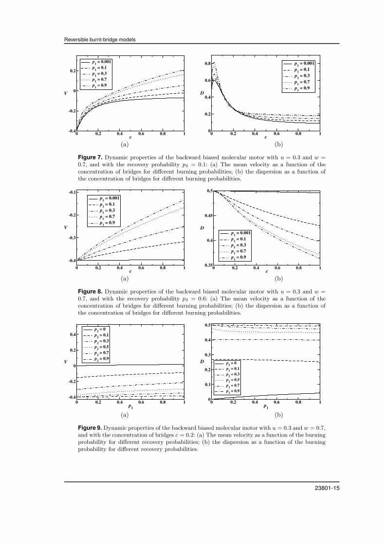
Figure 7. Dynamic properties of the backward biased molecular motor with u = 0.3 and w =0.7, and with the recovery probability p2 = 0.1: (a) The mean velocity as a function of theconcentration of bridges for different burning probabilities; (b) the dispersion as a function ofthe concentration of bridges for different burning probabilities.

(a) (b)

Figure 8. Dynamic properties of the backward biased molecular motor with u = 0.3 and w =0.7, and with the recovery probability p2 = 0.6: (a) The mean velocity as a function of theconcentration of bridges for different burning probabilities; (b) the dispersion as a function ofthe concentration of bridges for different burning probabilities.

(a) (b)

Figure 9. Dynamic properties of the backward biased molecular motor with u = 0.3 and w = 0.7,and with the concentration of bridges c = 0.2: (a) The mean velocity as a function of the burningprobability for different recovery probabilities; (b) the dispersion as a function of the burningprobability for different recovery probabilities.

23801-15


move in the opposite direction (figures 6–9). The analysis of dynamic properties shows that in thep2 → 1 limit (the deterministic bridge recovery) V → u − w = −0.4 and D → 1

2 (u + w) = 1/2for all c and p1 values (see figures 6 and 9), as it should be. The p1 → 0 limit in the u < w caseis more complex than in the u > w case (when V → u − w, D → 1

2 (u + w) for all p2 6= 0 andc values as p1 → 0). Namely, for u < w there exists p2(u, w) such that for non-zero p2 < p2 thedynamic properties V (c) and D(c) exhibit strong c-dependence in the p1 → 0 limit and they aredifferent from the u − w and 1

2 (u + w) values for non-zero c [figure 7 (a), (b)]. Exactly at p1 = 0(with p2 < p2), V (p1 = 0, c) = u − w and D(p1 = 0, c) = 1

2 (u + w) as obtained using the y = 1root of equation (22), given by equation (23) with “+” rather than “−” sign before the squareroot [the second root of equation (22)]. Thus for p2 < p2 there is a dynamic transition separatingp1 = 0 and p1 → 0 regimes. For u = 0.3, w = 0.7, it was found that p2 ≈ 0.57. For p2 > p2,V (p1 → 0, c) = V (p1 = 0, c) = u − w = −0.4 and D(p1 → 0, c) = D(p1 = 0, c) = 1

2 (u + w) = 0.5for all c values [figure 8 (a), (b)]. Physically this implies that bridges with arbitrarily low burningprobability strongly affect the dynamics of the particle which tends to move in the backwarddirection provided that the recovery probability p2 is less than some critical value; otherwise (inp2 > p2 case) weak links have no effect on the particle dynamics as p1 → 0. Thus in the p1 → 0limit there is a dynamic transition at p2 = p2 separating the regime with p2 < p2 when weak linksplay a role in the motor protein dynamics and the regime where they are irrelevant (p2 > p2). Itshould be noted that the p1 → 0 limit in figure 9 is in agreement with that in figures 7 and 8:p2 ≈ 0.57 plays the same role. The dynamic transition in the p1 → 0 limit also takes place forp2 = 0 (irreversible burning of weak connections). It separates backward biased p1 = 0 regime fromforward biased regime with small finite p1, when velocity V (c) is positive for all c > 0, althoughV (c) → 0, D(c) → 0 for all c values as p1 → 0 [see figure 9 (a), (b) with the specific c value]. Thereare therefore jumps in V (c) and D(c) at p1 = 0 for all p2 < p2 and all non-zero c.

Increasing the burning probability p1 and concentration of weak bonds c reduces the magnitudeof particle’s velocity in the backward direction; the same effect is observed when the recoveryprobability p2 is reduced, as expected [see figures 6 (a), 7 (a), 8 (a), 9 (a)]. For sufficiently large c,p1 (and small p2) the velocity V even becomes positive [figures 6 (a), 7 (a)]. We observed that forp2 = 0, V is always positive as the burning of weak bonds is irreversible in this case [figures 6 (a),9 (a)]. In that case, V (c = 0) = u−w is different from V (c → 0) = 0 [figure 6 (a)]. This effect wasalso observed in [9] in the p1 = 1 case.

Diffusion constant demonstrates a more complex behavior, with large fluctuations at small cand small p2 which increase with increasing p1 [figures 6 (b) and 7 (b)]. Figure 6(b) with p1 = 0.3is qualitatively similar to the corresponding figure in [9] with p1 = 1, although the maxima inD curves are less pronounced than in [9]. The shape of the D curve differs significantly betweenfigures 7 (b) and 8 (b) when the threshold p2 is crossed. In case of p2 = 0 (irreversible bridgeburning), fluctuations are reduced (especially at low c) and D curve differs substantially from non-zero p2 case [figures 6 (b) and 9(b)]. As was the case with the velocity, for p2 = 0 there is a gap inD separating D(c = 0) = 1

2 (u + w) from D(c → 0) = 0 [figure 6 (b)], again illustrating a dynamictransition. For non-zero p2 the diffusion constant is D(c → 0) = 1

2 (u + w), and there is no gap [seefigures 6 (b), 7 (b), 8 (b)].

5. Conclusions

We have presented a comprehensive theoretical method of calculating dynamic properties ofmolecular motors in reversible burnt-bridge models for periodic bridge distribution. It is a generali-zation of the approach developed by us in [6, 7] for the unbiased molecular motors and irreversibleburning of bridges. Exact and explicit expressions for mean velocity and dispersion have been de-rived for arbitrary values of parameters u, w, p1, p2 and c. In the known limiting cases of u = w = 1,p2 = 0 and of p1 = 1, we have reproduced our earlier findings [6, 7, 9], thereby confirming thevalidity of our theoretical analysis. Some interesting phenomena have been observed as a result ofthe investigation of dynamic properties of the molecular motor in BBM with bridge recovery. It in-cludes dynamic phase transitions and reversal of the direction of the motion. In case of the unbiased

23801-16


molecular motor, increasing the concentration of bridges c (or lowering the recovery probability p2)with other parameters kept fixed results in increasing velocity and decreasing dispersion. However,dependence of the dispersion on burning probability p1 is more complex; it is determined by thep2 value. In the limit of low c, gaps in dispersion plots have been observed for various p1 and p2

values, indicating the dynamic transition between biased and unbiased regimes. Also, a gap wasfound in the limit of small p1 between p2 = 0 and non-zero p2 regimes. Thus our results obtainedin [9] for p1 = 1 with u = w were generalized to cover the full range of p1 values.

For the backward biased molecular motor, increasing c has resulted in slowing down the back-ward movement of the particle, and for sufficiently small p2 (large p1) the direction of motion haseven been reversed and the velocity became positive. In the limit of small p1, a dynamic phasetransition separating p1 = 0 and p1 → 0 regimes has been found provided that p2 is less thansome critical value. For sufficiently small p2, broken bridges affect the particle’s dynamics evenif the burning probability p1 is infinitesimal. The behavior of dispersion as a function of c wasnon-monotonic for some range of parameters p1 and p2, with large fluctuations at small c andsmall p2. In the case of irreversible bridge burning (p2 = 0), we have observed gaps in velocity anddispersion in c → 0 limit (for p1 = 0.3), with the velocity being positive for all non-zero c values. Itsuggests that there is a dynamic transition at c = 0 separating backward biased and forward biaseddiffusion. The velocity and fluctuations are suppressed for sufficiently small c. Hence our findingsin [9] for u < w case with p1 = 1 have been extended to describe the general case of 0 < p1 6 1.

The method presented above applies to the case of periodic distribution of weak bonds, whichis probably realistic for collagenases [2]. As a problem to be addressed in the future studies, onecan consider BBM with random distribution of bridges [4, 5] where a different theoretical approachmust be applied.

References

1. Kolomeisky A.B., Fisher M.E., Ann. Rev. Phys. Chem., 2007, 58, 675.2. Saffarian S., Collier I.E., Marmer B.L., Elson E.L., Goldberg G., Science, 2004, 306, 108.3. Saffarian S., Qian H., Collier I.E., Elson E.L., Goldberg G., Phys. Rev. E, 2006, 73, 041909.4. Mai J., Sokolov I.M., Blumen A., Phys. Rev. E, 2001, 64, 011102.5. Antal T., Krapivsky P.L., Phys. Rev. E, 2005, 72, 046104.6. Morozov A.Y., Pronina E., Kolomeisky A.B., Artyomov M.N., Phys. Rev. E, 2007, 75, 031910.7. Artyomov M.N., Morozov A.Y., Pronina E., Kolomeisky A.B., J. Stat. Mech., 2007, P08002.8. Morozov A.Y., Kolomeisky A.B., J. Stat. Mech., 2007, P12008.9. Artyomov M.N., Morozov A.Y., Kolomeisky A.B., Phys. Rev. E, 2008, 77, 040901(R).

10. Derrida B., J. Stat. Phys., 1983, 31, 433.

23801-17


Динамiка молекулярних двигунiв у оборотнiй моделiспалених мостiв

М.Н. Артьомов1, А.Ю. Морозов2, А.Б. Коломейскi3

1 Хiмiчний факультет, Массачусеттський технологiчний iнститут, Кембрiдж, США2 Факультет фiзики i астрономiї, Унiверситет Калiфорнiї, Лос Анжелес, США3 Хiмiчний факультет, Унiверситет Райса, Г’юстон, США

Динамiчнi властивостi молекулярних двигунiв, чий рух здiйснюється завдяки взаємодiям з особли-вими ґратковими зв’язками, дослiджуються теоретично на основi стохастичних моделей “спалених

мостiв” з дискретними станами. Молекулярнi двигуни описуються як випадковi блукання, що можуть

знищувати чи вiдновлювати перiодично розподiленi зв’язки (“мости” при їх проходженнi з ймовiрно-стями, вiдповiдно, p1 та p2. Динамiчнi властивостi, такi як швидкостi та дисперсiї, отримуються в

точнiй та явнiй формi для довiльних значень параметрiв p1 i p2. Для неупередженого випадкового

блукання оборотне спалення мостiв приводить до упередженого спрямованого руху з динамiчним

переходом, що спостерiгається при дуже малих концентрацiях мостiв. У випадку упередженого мо-лекулярного двигуна, що може рухатись назад, його швидкiсть зменшується та змiна напрямку руху

спостерiгається для деякої областi параметрiв. Отримано також, що дисперсiя демонструє складну

немонотонну поведiнку з великими флуктуацiями для деякого набору параметрiв. Складна динамi-ка системи обговорюється за допомогою аналiзу поведiнки молекулярних двигунiв бiля спалених

мостiв.

Ключовi слова: молекулярнi двигуни, стохастичнi моделi, рухливi протеїни

23801-18

dynamics of molecular motors in reversible burnt-bridge...

Documents